Optimal Harvesting of a Semilinear Elliptic Logistic Fishery Model Wandi Ding 1 , Suzanne Lenhart 2 1 University of Tennessee - Knoxville, [email protected] 2 University of Tennessee - Knoxville & Oak Ridge National Laboratory Optimal Harvesting of a Semilinear Elliptic Logistic Fishery Model – p.1/21

Welcome message from author
This document is posted to help you gain knowledge. Please leave a comment to let me know what you think about it! Share it to your friends and learn new things together.
Transcript

Optimal Harvesting of aSemilinear Elliptic Logistic Fishery
ModelWandi Ding1, Suzanne Lenhart2
1University of Tennessee - Knoxville, [email protected] University of Tennessee - Knoxville & Oak Ridge National Laboratory
Optimal Harvesting of a Semilinear Elliptic Logistic Fishery Model – p.1/21
Outline• Development of Fishery Models• Motivation• The Model• Optimal Control Problems• Numerical Examples for J1
• Numerical Examples for J2
Optimal Harvesting of a Semilinear Elliptic Logistic Fishery Model – p.2/21
Development of Fishery Models[1]
• 1900 - 1920: First Efforts• F. I. Baranov: grandfather of fisheries
population dynamics• ICES (1902): International Council for the
Exploration of the Sea
[1] T. J. Quinn II, Ruminations on the Development and Future of Population Dynamics Models
in Fisheries, Natural Resource Modeling, 16:4, 2003
Optimal Harvesting of a Semilinear Elliptic Logistic Fishery Model – p.3/21

• 1920 - 1960: Establishment of Science• Ricker, Beverton and Holt, Leslie, Lotka and
Volterra, Thompson etc.• multi-species modeling,• age- and size-structure dynamics;
Optimal Harvesting of a Semilinear Elliptic Logistic Fishery Model – p.4/21

• 1960 - 1980: Deterministic Theory, StatisticalPractice• advances in age-structured models (Gulland,
Pope, Doubleday),
• improvements to surplus production (Pella,Tomlinson, Schnute, Fletcher, Hilborn) andstock recruitment models,
• bioeconomic models (Clark)• management control models (Hilborn,
Walters)
Optimal Harvesting of a Semilinear Elliptic Logistic Fishery Model – p.5/21

• 1980-2000: The Golden Age• integration between mathematics and statistics
• Bayesian and time series methods(uncertainty)
• realistic modeling for:· age and size-structured population· spatial dynamics· harvesting strategies(stochasticity, time variation)
Optimal Harvesting of a Semilinear Elliptic Logistic Fishery Model – p.6/21
• The New Millenium• future models:
• habitat and spatial concerns• genetics• multispecies interactions• enviromental factors• effects of harvesting on the ecosystem• socioeconomic concerns
Optimal Harvesting of a Semilinear Elliptic Logistic Fishery Model – p.7/21

MotivationNeubert(Ecology Letter, 2003) studied the fisherymanagement problem:Maximize the yield
J(h) =
∫
l
0
h(x)u(x) dx, 0 ≤ h(x) ≤ hmax
Subject to
−d2u
dx2= u(1 − u) − h(x)u, 0 < x < l,
u(0) = u(l) = 0.
Optimal Harvesting of a Semilinear Elliptic Logistic Fishery Model – p.8/21

Neubert’s Results• No-take marine reserves are always part of an
optimal harvest designed to maximize yield;
• The sizes and locations of the optimal reservesdepend on a dimensionless length parameter;
• For small values of this parameter, the maximumyield is obtained by placing a large reserve in thecenter of the habitat;
• For large values of this parameter, the optimalharvesting strategy is a spatial “chatteringcontrol” with infinite sequences of reservesalternating with areas of intense fishing;
Optimal Harvesting of a Semilinear Elliptic Logistic Fishery Model – p.9/21
Neubert’s Results• No-take marine reserves are always part of an
optimal harvest designed to maximize yield;• The sizes and locations of the optimal reserves
depend on a dimensionless length parameter;
• For small values of this parameter, the maximumyield is obtained by placing a large reserve in thecenter of the habitat;
• For large values of this parameter, the optimalharvesting strategy is a spatial “chatteringcontrol” with infinite sequences of reservesalternating with areas of intense fishing;
Optimal Harvesting of a Semilinear Elliptic Logistic Fishery Model – p.9/21

Neubert’s Results• No-take marine reserves are always part of an
optimal harvest designed to maximize yield;• The sizes and locations of the optimal reserves
depend on a dimensionless length parameter;• For small values of this parameter, the maximum
yield is obtained by placing a large reserve in thecenter of the habitat;
• For large values of this parameter, the optimalharvesting strategy is a spatial “chatteringcontrol” with infinite sequences of reservesalternating with areas of intense fishing;
Optimal Harvesting of a Semilinear Elliptic Logistic Fishery Model – p.9/21

Our Fishery Model
−∆u = ru(1 − u) − h(x)u, x ∈ Ω,
u = 0, x ∈ ∂Ω.
where u(x) is the fish density, r is the growth rate,
h(x) is the harvesting depending on the location of
fish, Ω ∈ Rn, smooth and bounded domain.
Optimal Harvesting of a Semilinear Elliptic Logistic Fishery Model – p.10/21

Optimal Control ProblemsGoals:
• Maximizing the yield and minimizing the cost offishing.
J1(h) =
∫
Ω
h(x)u(x) dx −
∫
Ω
(B1 + B2h)h dx,
h ∈ U1.
• Maximizing the yield and minimizing thevariation of the fishing effort.
J2(h) =
∫
Ω
h(x)u(x) dx−A
∫
Ω
|∇h|2 dx, h ∈ U2,
Optimal Harvesting of a Semilinear Elliptic Logistic Fishery Model – p.11/21

Optimality System Istate equation
−∆u = ru(1 − u) − h(x)u, x ∈ Ω,
u = 0, x ∈ ∂Ω;
adjoint equation
−∆p − r(1 − 2u)p + hp = h, x ∈ Ω,
p = 0, x ∈ ∂Ω;
characterization of optimal control
h(x) = minmax0,u − pu − B1
2B2
, 1 − δ.
Optimal Harvesting of a Semilinear Elliptic Logistic Fishery Model – p.12/21
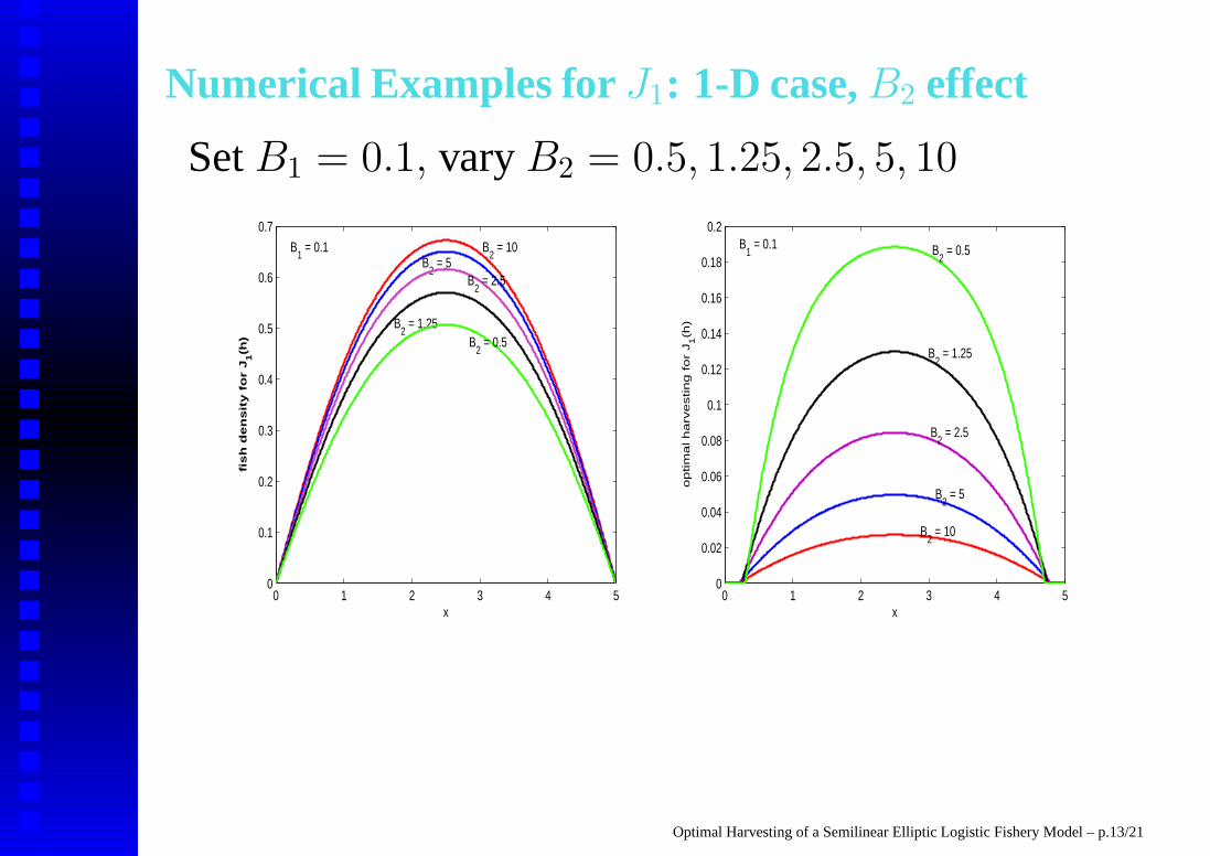
Numerical Examples for J1: 1-D case, B2 effect
Set B1 = 0.1, vary B2 = 0.5, 1.25, 2.5, 5, 10
0 1 2 3 4 50
0.1
0.2
0.3
0.4
0.5
0.6
0.7
x
fish
den
sit
y f
or
J1(h
)B
2 = 10
B2 = 5
B2 = 2.5
B2 = 1.25
B2 = 0.5
B1 = 0.1
0 1 2 3 4 50
0.02
0.04
0.06
0.08
0.1
0.12
0.14
0.16
0.18
0.2
x
optim
al harv
esting for
J1(h
)
B2 = 10
B2 = 5
B2 = 2.5
B2 = 1.25
B2 = 0.5B
1 = 0.1
Optimal Harvesting of a Semilinear Elliptic Logistic Fishery Model – p.13/21

Numerical Examples for J1: 1-D case, small B2
Set B1 = 0, vary B2 = 0.1, 0.05, 0.01
0 1 2 3 4 50
0.05
0.1
0.15
0.2
0.25
0.3
0.35
0.4
0.45
0.5
x
fish
den
sit
y f
or
J1(h
)
B2 = 0.1
B2 = 0.05
B2 = 0.01B
1 = 0
0 1 2 3 4 50
0.1
0.2
0.3
0.4
0.5
0.6
0.7
0.8
0.9
1
x
op
tim
al h
arv
esti
ng
fo
r J
1(h
)
B2 = 0.01
B2 = 0.05
B2 = 0.1
Optimal Harvesting of a Semilinear Elliptic Logistic Fishery Model – p.14/21

Numerical Examples for J1: 2-D case
00.5
11.5
22.5
0
1
2
30
0.1
0.2
0.3
0.4
0.5
x−axis
B1 = 0, B
2 = 1, r = 5, L = 2.5
y−axis
fish
den
sit
y f
or
J1(h
)
00.5
11.5
22.5
0
1
2
30
0.05
0.1
0.15
0.2
x−axis
B1 = 0, B
2 = 1, r = 5, L = 2.5
y−axis
op
tim
al h
arv
esti
ng
fo
r J
1(h
)
Optimal Harvesting of a Semilinear Elliptic Logistic Fishery Model – p.15/21

Numerical Examples for J1: 2-D case, B1 effect
00.5
11.5
22.5
0
1
2
30
0.05
0.1
0.15
0.2
x−axis
B1 = 0.1, B
2 = 1, r = 5, L = 2.5
y−axis
op
tim
al h
arv
esti
ng
fo
r J
1(h
)
00.5
11.5
22.5
0
1
2
30
0.05
0.1
0.15
0.2
x−axis
B1 = 0, B
2 = 1, r = 5, L = 2.5
y−axis
op
tim
al h
arv
esti
ng
fo
r J
1(h
)
Optimal Harvesting of a Semilinear Elliptic Logistic Fishery Model – p.16/21

Numerical Examples for J1: 2-D case, domain
size effect
0
1
2
3
0
1
2
30
0.2
0.4
0.6
0.8
x−axis
B1 = 0, B
2 = 1, r = 5, L = 3
y−axis
fish
den
sit
y f
or
J1(h
)
0
1
2
3
0
1
2
30
0.1
0.2
0.3
0.4
x−axis
B1 = 0, B
2 = 1, r = 5, L = 3
y−axis
op
tim
al h
arv
esti
ng
fo
r J
1(h
)
00.5
11.5
22.5
0
1
2
30
0.1
0.2
0.3
0.4
0.5
x−axis
B1 = 0, B
2 = 1, r = 5, L = 2.5
y−axis
fish
den
sit
y f
or
J1(h
)
00.5
11.5
22.5
0
1
2
30
0.05
0.1
0.15
0.2
x−axis
B1 = 0, B
2 = 1, r = 5, L = 2.5
y−axis
op
tim
al h
arv
esti
ng
fo
r J
1(h
)
Optimal Harvesting of a Semilinear Elliptic Logistic Fishery Model – p.17/21

Numerical Examples for J1: 2-D case, small B2
00.5
11.5
22.5
0
1
2
30
0.1
0.2
0.3
0.4
x−axis
B1 = 0, B
2 = 0.05, r = 5, L = 2.5
y−axis
fish
den
sit
y f
or
J1(h
)
00.5
11.5
22.5
0
1
2
30
0.2
0.4
0.6
0.8
1
x−axis
B1 = 0, B
2 = 0.05, r = 5, L = 2.5
y−axis
op
tim
al h
arv
esti
ng
fo
r J
1(h
)
Optimal Harvesting of a Semilinear Elliptic Logistic Fishery Model – p.18/21
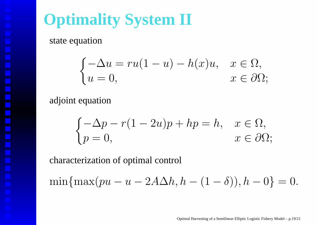
Optimality System IIstate equation
−∆u = ru(1 − u) − h(x)u, x ∈ Ω,
u = 0, x ∈ ∂Ω;
adjoint equation
−∆p − r(1 − 2u)p + hp = h, x ∈ Ω,
p = 0, x ∈ ∂Ω;
characterization of optimal control
minmax(pu − u − 2A∆h, h − (1 − δ)), h − 0 = 0.
Optimal Harvesting of a Semilinear Elliptic Logistic Fishery Model – p.19/21

Numerical Examples for J2:
Vary A = 1, 2.5, 5, 10
0 1 2 3 4 50
0.1
0.2
0.3
0.4
0.5
0.6
0.7
x
fish
den
sit
y f
or
J2(h
)
A=2.5
A=1
A=5A=10
0 1 2 3 4 50
0.05
0.1
0.15
0.2
0.25
0.3
0.35
x
op
tim
al h
arv
esti
ng
fo
r J
2(h
) A=1
A=5
A=10
A=2.5
Optimal Harvesting of a Semilinear Elliptic Logistic Fishery Model – p.20/21

Conclusion: in the long run• If we want to maximize yield and minimize cost
(J1),then increasing labor cost (B2) or fixed cost(B1) will decrease optimal harvesting;
• If we only want to maximize yield, then reserveis part of the optimal harvesting strategy;
• For J1, the optimal benefit inreases when domainsize increases;
• If we want to maximize yield and minimizevariation in fishing effort, then increasing (A)will reduce optimal harvesting.
Optimal Harvesting of a Semilinear Elliptic Logistic Fishery Model – p.21/21
Related Documents