Optimal Harvesting for a Predator–Prey Metapopulation

Bulletin of Mathematical Biology (1998) 60 (1): 49–65. http://dx.doi.org/10.1006/bulm.1997.0005

Optimal Harvesting for a Predator–Prey Metapopulation Asep K. Supriatna1 and Hugh P. Possingham2 1 Department of Applied Mathematics, University of Adelaide, SA 5005 Australia 2 Department of Environmental Science and Management, University of Adelaide, Roseworthy SA 5371 Australia Abstract

In this paper we present a deterministic, discrete-time model for a two-patch predator–prey metapopulation. We study optimal harvesting for the metapopulation using dynamic programming. Some rules are established as generalizations of rules for a single-species metapopulation harvesting theory. We also establish rules to harvest relatively more (or less) vulnerable prey subpopulations and more (or less) efficient predator subpopulations. 1. Introduction

All marine populations show some degree of spatial heterogeneity. Sometimes this spatial heterogeneity means that modelling the species as one single population is not adequate. For example, abalone, Haliotis rubra, has a discrete metapopulation structure with local populations connected by the dispersal of their larvae (Prince et al., 1987; Prince 1992). Brown and Murray (1992) and Shepherd and Brown (1993) argue that management for abalone should depend on the characteristics of local populations. Frank (1992) provides another example of the metapopulation structure. He points out that fish stocks, such as the cod of Iceland and West Greenland, which are separated by a large distance, and the two haddock stocks of the Scotian Shelf, are known to be strongly coupled by the dispersal of individuals. He also suggests that those stocks possess the ‘source/sink’ property described by Sinclair (1988) and Pulliam (1988), that is, persistence of the population in a sink habitat can be maintained by the migration from a source habitat. Source/sink habitat will be defined precisely in the next section. Furthermore, Frank and Leggett (1994) argue that the collapse of major fisheries such as North Atlantic Cod and Atlantic and Pacific Salmon, is due to the over-exploitation of the source population.

Despite the importance of spatial heterogeneity, increasing the complexity of a population

model by adding spatial heterogeneity is rarely done in fishery y management modeling, even for single species (Clark, 1984). Exceptions are Clark (1976), Tuck and Possingham (1994) and Brown and Roughgarden (1997) for a single species, and Hilborn and Walters (1987), Leung (1995), and Murphy (1995) for multiple species. In this paper we present a model for a spatially structured predator–prey population. We address the issues of spatial structure and predator–prey interaction, and study optimal harvesting for the metapopu-lation. We use metapopulation theory to describe the spatial structure of the predator–prey system. Using this approach, we obtain the optimal harvest for each local population which gives important information on how we should harvest a population if management can be specified for local populations, such as abalone.

2. The Model

This section describes a deterministic, discrete-time model for a spatially structured predator–prey system. The model has similar structure and assumptions to that described in Tuck and Possingham (1994).

Assume that there is a predator–prey population in each of two different patches, namely patch 1 and patch 2. Let the movement of individuals between the local populations be


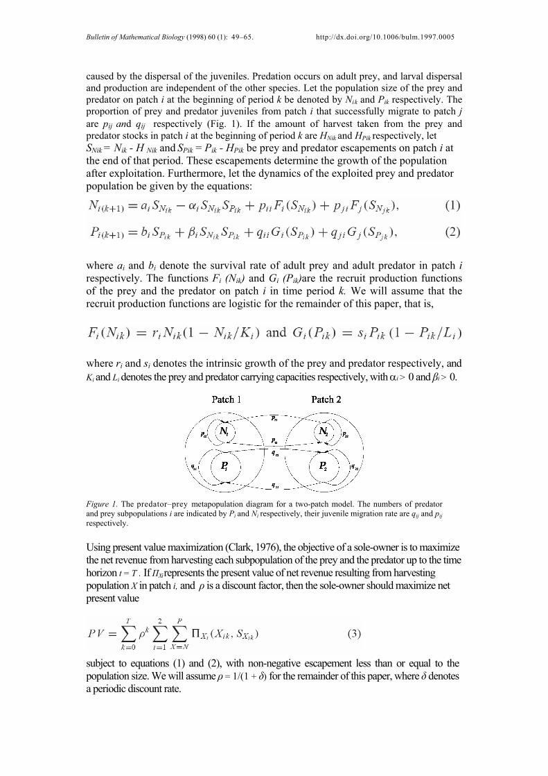
caused by the dispersal of the juveniles. Predation occurs on adult prey, and larval dispersal and production are independent of the other species. Let the population size of the prey and predator on patch i at the beginning of period k be denoted by Nik and Pik respectively. The proportion of prey and predator juveniles from patch i that successfully migrate to patch j are pij and qij respectively (Fig. 1). If the amount of harvest taken from the prey and predator stocks in patch i at the beginning of period k are HNik and HPik respectively, let SNik = Nik - H Nik and SPik = Pik - HPik be prey and predator escapements on patch i at the end of that period. These escapements determine the growth of the population after exploitation. Furthermore, let the dynamics of the exploited prey and predator population be given by the equations:

where ai and bi denote the survival rate of adult prey and adult predator in patch i respectively. The functions Fi (Nik) and Gi (Pik)are the recruit production functions of the prey and the predator on patch i in time period k. We will assume that the recruit production functions are logistic for the remainder of this paper, that is,

where ri and si denotes the intrinsic growth of the prey and predator respectively, and Ki and Li denotes the prey and predator carrying capacities respectively, with αi > 0 and βi > 0.

Figure 1. The predator–prey metapopulation diagram for a two-patch model. The numbers of predator and prey subpopulations i are indicated by Pi and Ni respectively, their juvenile migration rate are qij and pij respectively. Using present value maximization (Clark, 1976), the objective of a sole-owner is to maximize the net revenue from harvesting each subpopulation of the prey and the predator up to the time horizon t = T . If ΠXi represents the present value of net revenue resulting from harvesting population X in patch i, and ρ is a discount factor, then the sole-owner should maximize net present value

subject to equations (1) and (2), with non-negative escapement less than or equal to the population size. We will assume ρ = 1/(1 + δ) for the remainder of this paper, where δ denotes a periodic discount rate.


If there is no discount rate (δ = 0) then the net revenue (3) in any period generated by escapements SNi and SPi has exactly the same value to the net revenue from the same escapements in any other periods. Hence, we only need to find optimal escapements for one period to go. The resulting revenue by applying this zero discount rate is often known as maximum economic yield (MEY). If the discount rate is extremely high (δ ) then the net revenue (3) approaches

which is the immediate net revenue without considering the future and is maximized by optimal escapements S*Xi We use the symbol ‘ ’ to indicate that the exploiter only cares about profit this period, which is the same as applying the large discount rate δ . It can be regarded as an open-access exploitation.

The net revenue for a two-patch predator–prey population from the harvest HXik of the sub-population Xi in period k is

where pX is the price of the harvested stock X and is assumed to be constant, while cXi is the unit cost of harvesting and is assumed to be a non-increasing function of Xi and may depend on the location of the stock. To obtain the optimal harvest for a two-patch predator–prey population we define a value function

which is the sum of the discounted net revenue resulting from harvesting both populations in both locations up to period t = T . This function is maximized by choosing appropriate optimal escapements S*Xik. Equation (6) is used recursively to obtain the value function at time T + 1, that is

Thus the optimal escapements, S*Ni0 and S*Pi0, for a two-patch predator–prey system can be found by iterating this equation back from time T.

First, consider the net revenue in equation (6) for time horizon T = 0. The resulting net revenue, J0(N10, N20, P10, P20), represents immediate net revenue taken from the next harvest without considering the future value of the harvest, hence the maximum value is exactly the same as the maximum value of PV , in (4). We consider two cases. Case 1. If the unit cost of harvesting is constant, let cXi (Xi) = cXi , then pX –cXi in (5) is constant. Hence, the integral in (5), and thus PV , in (4), is maximized by S*Xi , satisfying


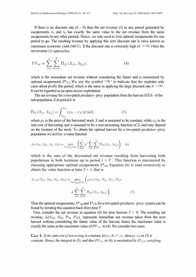
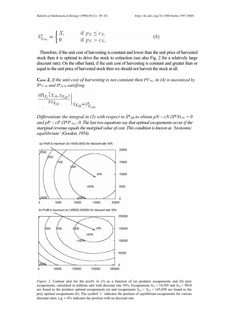
Therefore, if the unit cost of harvesting is constant and lower than the unit price of harvested stock then it is optimal to drive the stock to extinction (see also Fig. 2 for a relatively large discount rate). On the other hand, if the unit cost of harvesting is constant and greater than or equal to the unit price of harvested stock then we should not harvest the stock at all.

Case 2. If the unit cost of harvesting is not constant then PV , in (4) is maximized by S*Ni and S*Pi satisfying

Differentiate the integral in (5) with respect to S*Xi0 to obtain pN − cN (S*Ni = 0 and pP − cP (S*P ) = 0. The last two equations say that optimal escapements occur if the marginal revenue equals the marginal value of cost. This condition is known as ‘bionomic equilibrium’ (Gordon, 1954).

Figure 2. Contour plot for the profit in (3) as a function of (a) predator escapements and (b) prey escapements, calculated in millions unit with discount rate 10%. Escapements SP1

= 14,505 and SP2 = 9010

are found as the predator optimal escapements (a) and escapements SN1 = SN2 = 145,050 are found as the

prey optimal escapements (b). The symbol ‘×’ indicates the position of equilibrium escapements for various discount rates, e.g. × 0% indicates the position with no discount rate.


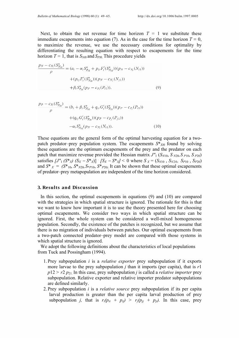
Next, to obtain the net revenue for time horizon T = 1 we substitute these immediate escapements into equation (7). As in the case for the time horizon T = 0, to maximize the revenue, we use the necessary conditions for optimality by differentiating the resulting equation with respect to escapements for the time horizon T = 1, that is SNi0 and SPi0. This procedure yields

These equations are the general form of the optimal harvesting equation for a two-patch predator–prey population system. The escapements S*Xi0 found by solving these equations are the optimum escapements of the prey and the predator on each patch that maximize revenue provided the Hessian matrix J"1 (SN10, S N20,S P10, S P20) satisfies [J"1 (S*X) (SX − S*X)] . [SX − S*X] < 0 where S X = (SN10 , SN20, SP10 , SP20) and S* X = (S*10, S*N20,S*P10, S*P20). It can be shown that these optimal escapements of predator–prey metapopulation are independent of the time horizon considered.

3. Results and Discussion

In this section, the optimal escapements in equations (9) and (10) are compared with the strategies in which spatial structure is ignored. The rationale for this is that we want to know how important it is to use the theory presented here for choosing optimal escapements. We consider two ways in which spatial structure can be ignored. First, the whole system can be considered a well-mixed homogeneous population. Secondly, the existence of the patches is recognized, but we assume that there is no migration of individuals between patches. Our optimal escapements from a two-patch connected predator–prey model are compared with those systems in which spatial structure is ignored.

We adopt the following definitions about the characteristics of local populations from Tuck and Possingham (1994).

1. Prey subpopulation i is a relative exporter prey subpopulation if it exports more larvae to the prey subpopulation j than it imports (per capita), that is r1 p12 > r2 p21. In this case, prey subpopulation j is called a relative importer prey subpopulation. Relative exporter and relative importer predator subpopulations are defined similarly.

2. Prey subpopulation i is a relative source prey subpopulation if its per capita larval production is greater than the per capita larval production of prey subpopulation j, that is ri(pii + pij) > rj(pjj + pji). In this case, prey


subpopulation j is called a relative sink subpopulation. Relative source and relative sink predator subpopulations are defined similarly.

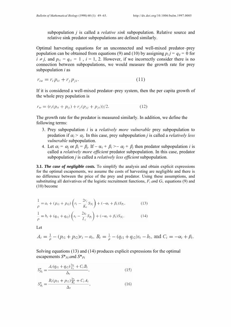
Optimal harvesting equations for an unconnected and well-mixed predator–prey population can be obtained from equations (9) and (10) by assigning pi j = qij = 0 for i ≠ j, and pii = qii = 1 , i = 1, 2. However, if we incorrectly consider there is no connection between subpopulations, we would measure the growth rate for prey subpopulation i as

If it is considered a well-mixed predator–prey system, then the per capita growth of the whole prey population is

The growth rate for the predator is measured similarly. In addition, we define the following terms:

3. Prey subpopulation i is a relatively more vulnerable prey subpopulation to predation if αi > αj. In this case, prey subpopulation j is called a relatively less vulnerable subpopulation.

4. Let αi = αj or βi = βj. If − αi + βi >− αj + βj then predator subpopulation i is called a relatively more efficient predator subpopulation. In this case, predator subpopulation j is called a relatively less efficient subpopulation.

3.1. The case of negligible costs. To simplify the analysis and obtain explicit expressions for the optimal escapements, we assume the costs of harvesting are negligible and there is no difference between the price of the prey and predator. Using these assumptions, and substituting all derivatives of the logistic recruitment functions, Fi and Gi, equations (9) and (10) become

Let

Solving equations (13) and (14) produces explicit expressions for the optimal escapements S*Ni and S*Pi


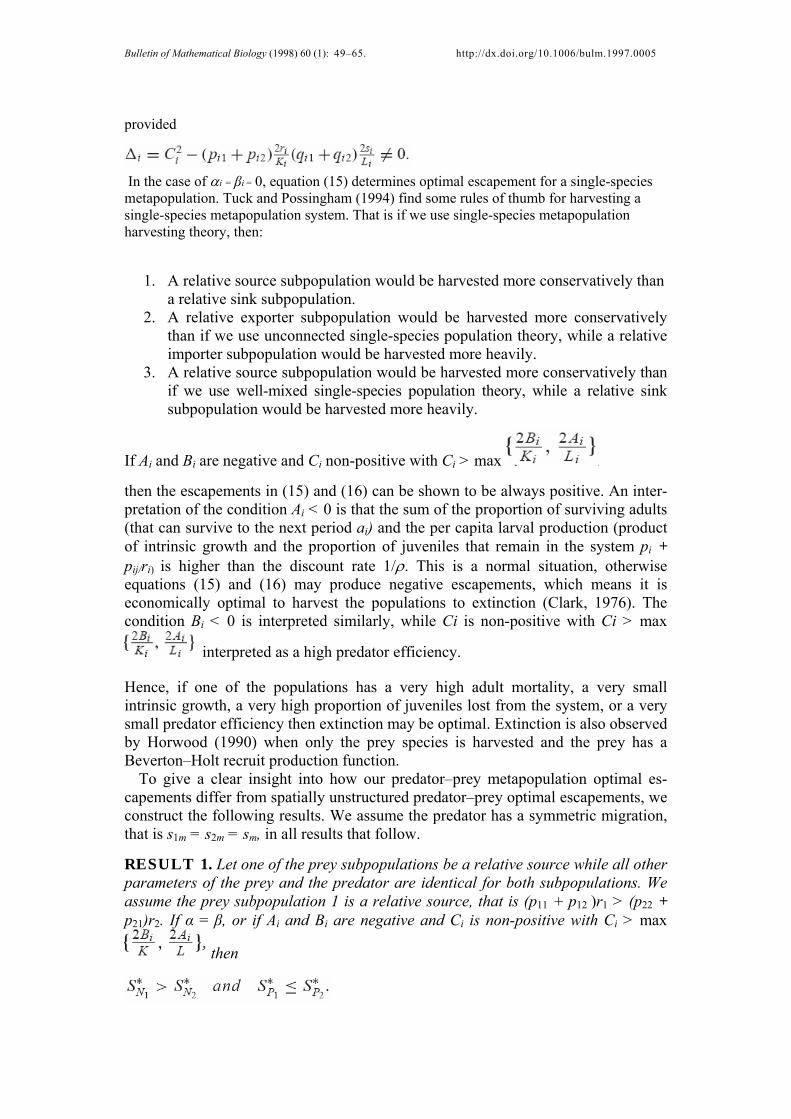
provided

In the case of αi = βi = 0, equation (15) determines optimal escapement for a single-species metapopulation. Tuck and Possingham (1994) find some rules of thumb for harvesting a single-species metapopulation system. That is if we use single-species metapopulation harvesting theory, then:

1. A relative source subpopulation would be harvested more conservatively than

a relative sink subpopulation. 2. A relative exporter subpopulation would be harvested more conservatively

than if we use unconnected single-species population theory, while a relative importer subpopulation would be harvested more heavily.

3. A relative source subpopulation would be harvested more conservatively than if we use well-mixed single-species population theory, while a relative sink subpopulation would be harvested more heavily.

If Ai and Bi are negative and Ci non-positive with Ci > max

then the escapements in (15) and (16) can be shown to be always positive. An inter-pretation of the condition Ai < 0 is that the sum of the proportion of surviving adults (that can survive to the next period ai) and the per capita larval production (product of intrinsic growth and the proportion of juveniles that remain in the system pi + pij/ri) is higher than the discount rate 1/ρ. This is a normal situation, otherwise equations (15) and (16) may produce negative escapements, which means it is economically optimal to harvest the populations to extinction (Clark, 1976). The condition Bi < 0 is interpreted similarly, while Ci is non-positive with Ci > max

interpreted as a high predator efficiency.

Hence, if one of the populations has a very high adult mortality, a very small intrinsic growth, a very high proportion of juveniles lost from the system, or a very small predator efficiency then extinction may be optimal. Extinction is also observed by Horwood (1990) when only the prey species is harvested and the prey has a Beverton–Holt recruit production function.

To give a clear insight into how our predator–prey metapopulation optimal es-capements differ from spatially unstructured predator–prey optimal escapements, we construct the following results. We assume the predator has a symmetric migration, that is s1m = s2m = sm, in all results that follow.

RESULT 1. Let one of the prey subpopulations be a relative source while all other parameters of the prey and the predator are identical for both subpopulations. We assume the prey subpopulation 1 is a relative source, that is (p11 + p12 )r1 > (p22 + p21)r2. If α = β, or if Ai and Bi are negative and Ci is non-positive with Ci > max

then


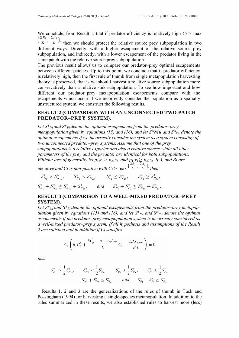
We conclude, from Result 1, that if predator efficiency is relatively high Ci > max

then we should protect the relative source prey subpopulation in two different ways. Directly, with a higher escapement of the relative source prey subpopulation, and indirectly, with a lower escapement of the predator living in the same patch with the relative source prey subpopulation. The previous result allows us to compare our predator–prey optimal escapements between different patches. Up to this point, we conclude that if predator efficiency is relatively high, then the first rule of thumb from single metapopulation harvesting theory is preserved, that is we should harvest a relative source subpopulation more conservatively than a relative sink subpopulation. To see how important and how different our predator–prey metapopulation escapements compare with the escapements which occur if we incorrectly consider the population as a spatially unstructured system, we construct the following results.

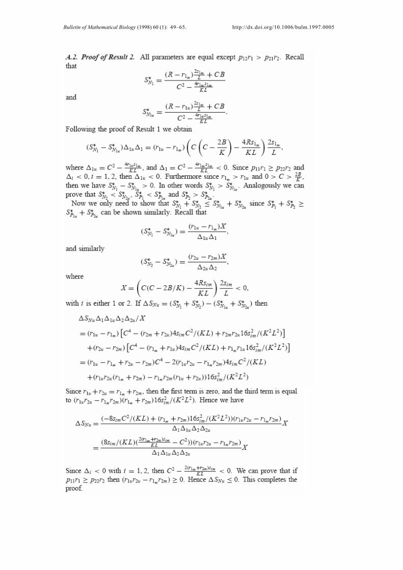
RESULT 2 (COMPARISON WITH AN UNCONNECTED TWO-PATCH PREDATOR–PREY SYSTEM).

Let S*Ni and S*Pi denote the optimal escapements from the predator–prey metapopulation given by equations (15) and (16), and let S*Niu and S*Piu denote the optimal escapements if we incorrectly consider the system as a system consisting of two unconnected predator–prey systems. Assume that one of the prey subpopulations is a relative exporter and also a relative source while all other parameters of the prey and the predator are identical for both subpopulations. Without loss of generality let p12r1 > p21r2 and p11r1 ≥ p22r2. If Ai and Bi are

negative and Ci is non-positive with Ci > max then

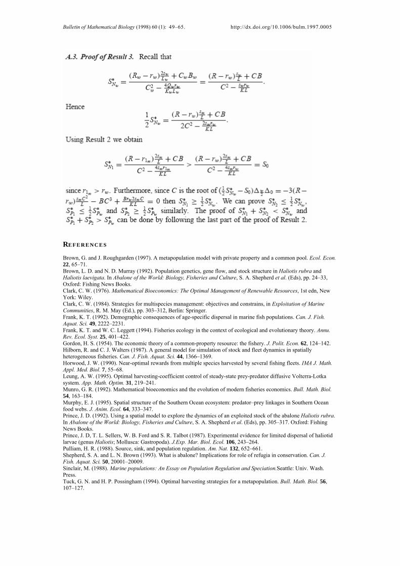
RESULT 3 (COMPARISON TO A WELL-MIXED PREDATOR–PREY SYSTEM). Let S*Ni and S*Pi denote the optimal escapements from the predator–prey metapop-ulation given by equations (15) and (16), and let S*Nw and S*Pw denote the optimal escapements if the predator–prey metapopulation system is incorrectly considered as a well-mixed predator–prey system. If all hypothesis and assumptions of the Result 2 are satisfied and in addition if Ci satisfies

Results 1, 2 and 3 are the generalizations of the rules of thumb in Tuck and Possingham (1994) for harvesting a single-species metapopulation. In addition to the rules summarized in these results, we also established rules to harvest more (less)


vulnerable prey and more (less) efficient predator subpopulations. These rules are summarized in the following result.

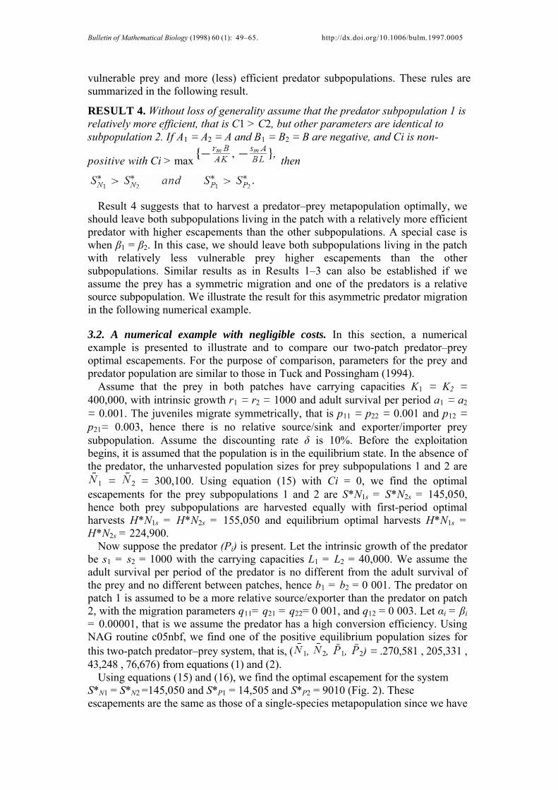
RESULT 4. Without loss of generality assume that the predator subpopulation 1 is relatively more efficient, that is C1 > C2, but other parameters are identical to subpopulation 2. If A1 = A2 = A and B1 = B2 = B are negative, and Ci is non-

positive with Ci > max then

Result 4 suggests that to harvest a predator–prey metapopulation optimally, we should leave both subpopulations living in the patch with a relatively more efficient predator with higher escapements than the other subpopulations. A special case is when β1 = β2. In this case, we should leave both subpopulations living in the patch with relatively less vulnerable prey higher escapements than the other subpopulations. Similar results as in Results 1–3 can also be established if we assume the prey has a symmetric migration and one of the predators is a relative source subpopulation. We illustrate the result for this asymmetric predator migration in the following numerical example.

3.2. A numerical example with negligible costs. In this section, a numerical example is presented to illustrate and to compare our two-patch predator–prey optimal escapements. For the purpose of comparison, parameters for the prey and predator population are similar to those in Tuck and Possingham (1994).

Assume that the prey in both patches have carrying capacities K1 = K2 = 400,000, with intrinsic growth r1 = r2 = 1000 and adult survival per period a1 = a2 = 0.001. The juveniles migrate symmetrically, that is p11 = p22 = 0.001 and p12 = p21= 0.003, hence there is no relative source/sink and exporter/importer prey subpopulation. Assume the discounting rate δ is 10%. Before the exploitation begins, it is assumed that the population is in the equilibrium state. In the absence of the predator, the unharvested population sizes for prey subpopulations 1 and 2 are

1 = 2 = 300,100. Using equation (15) with Ci = 0, we find the optimal escapements for the prey subpopulations 1 and 2 are S*N1s = S*N2s = 145,050, hence both prey subpopulations are harvested equally with first-period optimal harvests H*N1s = H*N2s = 155,050 and equilibrium optimal harvests H*N1s = H*N2s = 224,900.

Now suppose the predator (Pi) is present. Let the intrinsic growth of the predator be s1 = s2 = 1000 with the carrying capacities L1 = L2 = 40,000. We assume the adult survival per period of the predator is no different from the adult survival of the prey and no different between patches, hence b1 = b2 = 0 001. The predator on patch 1 is assumed to be a more relative source/exporter than the predator on patch 2, with the migration parameters q11= q21 = q22= 0 001, and q12 = 0 003. Let αi = βi = 0.00001, that is we assume the predator has a high conversion efficiency. Using NAG routine c05nbf, we find one of the positive equilibrium population sizes for this two-patch predator–prey system, that is, ( 1, 2, 1, 2) = .270,581 , 205,331 , 43,248 , 76,676) from equations (1) and (2).

Using equations (15) and (16), we find the optimal escapement for the system S*N1 = S*N2 =145,050 and S*P1 = 14,505 and S*P2 = 9010 (Fig. 2). These escapements are the same as those of a single-species metapopulation since we have


αi = βi for each patch. However, the optimal harvests are different. In this case, we find the first period optimal harvests H*N1 = 125,531, H*N2 = 60,281, H*P1 = 28,743, H*P2 = 6766, and the equilibrium optimal harvests H*N1 = 203,861, H*N2 = 211,831, H*P1 = 22,775, and H*P2 = 38,784. As expected, because there is no source/sink or exporter/importer prey subpopulation, using both methods we harvest predator subpopulation 1 more conservatively than predator subpopulation 2. In this case H*P1 = 22,775 and H*P2 = 38,784 from two-patch predator– prey escapements, while H*P1s = 1735 and H*P2s = 25,715 from single-species metapopulation escapements.

Even though the degree of predator–prey interaction is very low, that is small α and small β, optimal harvests from a single-species metapopulation and from a predator–prey metapopulation can be very different quantitatively. In general, if Ci ≤ 0, then the optimal escapement from a predator–prey metapopulation is less than or equal to optimal escapement from a single-species metapopulation. As a result, if we use optimal escapement from a single-species metapopulation as a policy to manage a predator–prey metapopulation system, then we might under harvest the stocks. On the other hand, if we use optimal harvest from a single metapopulation, we might over harvest the prey and under harvest the predator. Next, we compare the optimal escapements and equilibrium harvests from a predator–prey metapopulation to the optimal escapements and equilibrium harvests if spatial structure is not considered in the system.

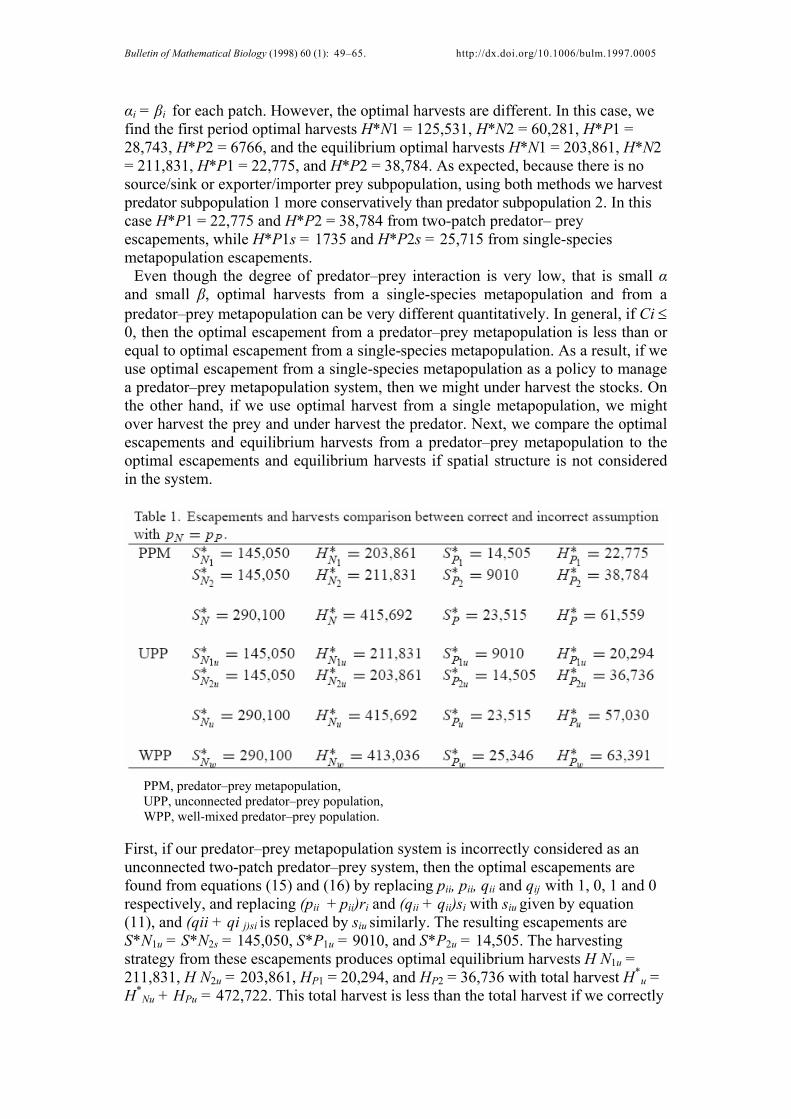
PPM, predator–prey metapopulation, UPP, unconnected predator–prey population, WPP, well-mixed predator–prey population.

First, if our predator–prey metapopulation system is incorrectly considered as an unconnected two-patch predator–prey system, then the optimal escapements are found from equations (15) and (16) by replacing pii, pii, qii and qij with 1, 0, 1 and 0 respectively, and replacing (pii + pii)ri and (qii + qii)si with siu given by equation (11), and (qii + qi j)si is replaced by siu similarly. The resulting escapements are S*N1u = S*N2s = 145,050, S*P1u = 9010, and S*P2u = 14,505. The harvesting strategy from these escapements produces optimal equilibrium harvests H N1u = 211,831, H N2u = 203,861, HP1 = 20,294, and HP2 = 36,736 with total harvest H*

u = H*

Nu + HPu = 472,722. This total harvest is less than the total harvest if we correctly


use a predator–prey metapopulation escapements, that is H* = H*N + H*

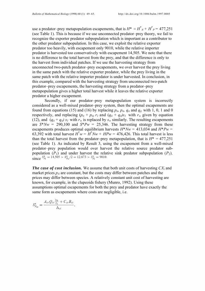
P = 477,251 (see Table 1). This is because if we use unconnected predator–prey theory, we fail to recognize the exporter predator subpopulation which is important as a contributor to the other predator subpopulation. In this case, we exploit the relative exporter predator too heavily, with escapement only 9010, while the relative importer predator is harvested too conservatively with escapement 14,505. We note that there is no difference to the total harvest from the prey, and that the difference is only to the harvest from individual patches. If we use the harvesting strategy from unconnected two-patch predator–prey escapements, we over harvest the prey living in the same patch with the relative exporter predator, while the prey living in the same patch with the relative importer predator is under harvested. In conclusion, in this example, compared with the harvesting strategy from unconnected two-patch predator–prey escapements, the harvesting strategy from a predator–prey metapopulation gives a higher total harvest while it leaves the relative exporter predator a higher escapement. Secondly, if our predator–prey metapopulation system is incorrectly considered as a well-mixed predator–prey system, then the optimal escapements are found from equations (15) and (16) by replacing pii, pii, qii and qij with 1, 0, 1 and 0 respectively, and replacing (pii + pii) r1 and (qii + qii)s1 with rw given by equation (12), and (qii + qii) s1 with rw is replaced by sw similarly. The resulting escapements are S*Nw = 290,100 and S*Pw = 25,346. The harvesting strategy from these escapements produces optimal equilibrium harvests H*Nw = 413,034 and H*Pw = 63,392 with total harvest H*w = H*Nw + HPw = 476,426. This total harvest is less than the total harvest from the predator–prey metapopulation, that is H* = 477,251 (see Table 1). As indicated by Result 3, using the escapement from a well-mixed predator–prey population would over harvest the relative source predator sub-population (P1) and under harvest the relative sink predator subpopulation (P2), since The case of cost inclusion. We assume that both unit costs of harvesting CXi and market prices pX are constant, but the costs may differ between patches and the prices may differ between species. A relatively constant unit cost of harvesting are known, for example, in the clupeoids fishery (Munro, 1992). Using these assumptions optimal escapements for both the prey and predator have exactly the same form as escapements where costs are negligible, i.e.


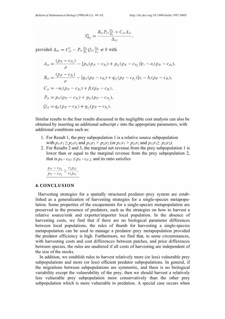
Similar results to the four results discussed in the negligible cost analysis can also be obtained by inserting an additional subscript c into the appropriate parameters, with additional conditions such as:

1. For Result 1, the prey subpopulation 1 is a relative source subpopulation with p11r1 ≥ p21r2 and p12r1 > p22r2 (or p11r1 > p21r2 and p12r1≥ p22r2).

2. For Results 2 and 3, the marginal net revenue from the prey subpopulation 1 is lower than or equal to the marginal revenue from the prey subpopulation 2, that is pN - cN1 ≤ pN - cN 2, and its ratio satisfies

4. CONCLUSION

Harvesting strategies for a spatially structured predator–prey system are estab-lished as a generalization of harvesting strategies for a single-species metapopu-lation. Some properties of the escapements for a single-species metapopulation are preserved in the presence of predators, such as the strategies on how to harvest a relative source/sink and exporter/importer local population. In the absence of harvesting costs, we find that if there are no biological parameter differences between local populations, the rules of thumb for harvesting a single-species metapopulation can be used to manage a predator–prey metapopulation provided the predator efficiency is high. Furthermore, we find that, in some circumstances, with harvesting costs and cost differences between patches, and price differences between species, the rules are unaltered if all costs of harvesting are independent of the size of the stocks.

In addition, we establish rules to harvest relatively more (or less) vulnerable prey subpopulations and more (or less) efficient predator subpopulations. In general, if the migrations between subpopulations are symmetric, and there is no biological variability except the vulnerability of the prey, then we should harvest a relatively less vulnerable prey subpopulation more conservatively than the other prey subpopulation which is more vulnerable to predation. A special case occurs when


there is no predation in patch 1, that is α1 = β1 = 0. In this case, patch 1 is a refuge for the prey. We find that the prey living in their refugial habitat should be harvested more conservatively than the prey living in the habitat where predation occurs. Similarly, if the only biological variability is the predator efficiency, then we should harvest the prey living in the same patch with the relatively more efficient predator more conservatively than the other prey subpopulation. Furthermore, if both prey vulnerability and predator efficiency vary between patches, unlike predator efficiency, prey vulnerability does not have any significant effect on the optimal escapements. In this case, we harvest a relatively more efficient predator more conservatively than a relatively less efficient predator. We also harvest the prey living in the same patch with the relatively more efficient predator more conservatively.

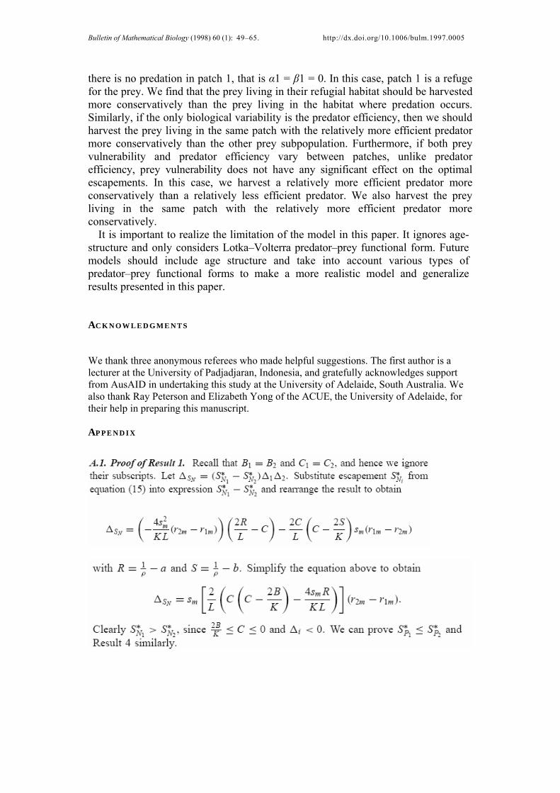
It is important to realize the limitation of the model in this paper. It ignores age-structure and only considers Lotka–Volterra predator–prey functional form. Future models should include age structure and take into account various types of predator–prey functional forms to make a more realistic model and generalize results presented in this paper. AC K N O W L E D G M E N T S

We thank three anonymous referees who made helpful suggestions. The first author is a lecturer at the University of Padjadjaran, Indonesia, and gratefully acknowledges support from AusAID in undertaking this study at the University of Adelaide, South Australia. We also thank Ray Peterson and Elizabeth Yong of the ACUE, the University of Adelaide, for their help in preparing this manuscript. AP P E N D I X



RE F E R E N C E S Brown, G. and J. Roughgarden (1997). A metapopulation model with private property and a common pool. Ecol. Econ. 22, 65–71. Brown, L. D. and N. D. Murray (1992). Population genetics, gene flow, and stock structure in Haliotis rubra and Haliotis laevigata. In Abalone of the World: Biology, Fisheries and Culture, S. A. Shepherd et al. (Eds), pp. 24–33, Oxford: Fishing News Books. Clark, C. W. (1976). Mathematical Bioeconomics: The Optimal Management of Renewable Resources, 1st edn, New York: Wiley. Clark, C. W. (1984). Strategies for multispecies management: objectives and constrains, in Exploitation of Marine Communities, R. M. May (Ed.), pp. 303–312, Berlin: Springer. Frank, K. T. (1992). Demographic consequences of age-specific dispersal in marine fish populations. Can. J. Fish. Aquat. Sci. 49, 2222–2231. Frank, K. T. and W. C. Leggett (1994). Fisheries ecology in the context of ecological and evolutionary theory. Annu. Rev. Ecol. Syst. 25, 401–422. Gordon, H. S. (1954). The economic theory of a common-property resource: the fishery. J. Polit. Econ. 62, 124–142. Hilborn, R. and C. J. Walters (1987). A general model for simulation of stock and fleet dynamics in spatially heterogeneous fisheries. Can. J. Fish. Aquat. Sci. 44, 1366–1369. Horwood, J. W. (1990). Near-optimal rewards from multiple species harvested by several fishing fleets. IMA J. Math. Appl. Med. Biol. 7, 55–68. Leung, A. W. (1995). Optimal harvesting-coefficient control of steady-state prey-predator diffusive Volterra-Lotka system. App. Math. Optim. 31, 219–241. Munro, G. R. (1992). Mathematical bioeconomics and the evolution of modern fisheries economics. Bull. Math. Biol. 54, 163–184. Murphy, E. J. (1995). Spatial structure of the Southern Ocean ecosystem: predator–prey linkages in Southern Ocean food webs. J. Anim. Ecol. 64, 333–347. Prince, J. D. (1992). Using a spatial model to explore the dynamics of an exploited stock of the abalone Haliotis rubra. In Abalone of the World: Biology, Fisheries and Culture, S. A. Shepherd et al. (Eds), pp. 305–317. Oxford: Fishing News Books. Prince, J. D, T. L. Sellers, W. B. Ford and S. R. Talbot (1987). Experimental evidence for limited dispersal of haliotid larvae (genus Haliotis; Mollusca: Gastropoda). J.Exp. Mar. Biol. Ecol. 106, 243–264. Pulliam, H. R. (1988). Source, sink, and population regulation. Am. Nat. 132, 652–661. Shepherd, S. A. and L. N. Brown (1993). What is abalone? Implications for role of refugia in conservation. Can. J. Fish. Aquat. Sci. 50, 20001–20009. Sinclair, M. (1988). Marine populations: An Essay on Population Regulation and Speciation.Seattle: Univ. Wash. Press. Tuck, G. N. and H. P. Possingham (1994). Optimal harvesting strategies for a metapopulation. Bull. Math. Biol. 56, 107–127.


Optimal Harvesting for a Predator–Prey Metapopulation

Documents