Optimal football strategies: AC Milan versus FC Barcelona - Munich

MPRAMunich Personal RePEc Archive

Optimal football strategies: AC Milanversus FC Barcelona

Christos Papahristodoulou

Malardalen University/Industrial Economics

January 2012

Online at http://mpra.ub.uni-muenchen.de/35940/MPRA Paper No. 35940, posted 14. January 2012 21:22 UTC

Optimal football strategies: AC Milan versus FC Barcelona

Christos Papahristodoulou*

Abstract

In a recent UEFA Champions League game between AC Milan and FC Barcelona,

played in Italy (final score 2-3), the collected match statistics, classified into four

offensive and two defensive strategies, were in favour of FC Barcelona (by 13 versus

8 points). The aim of this paper is to examine to what extent the optimal game

strategies derived from some deterministic, possibilistic, stochastic and fuzzy LP

models would improve the payoff of AC Milan at the cost of FC Barcelona.

Keywords: football game, mixed strategies, fuzzy, stochastic, Nash equilibria

*Department of Industrial Economics, Mälardalen University, Västerås, Sweden;

[email protected] Tel; +4621543176

2

1. Introduction The main objective of the teams’ managers is to find their optimal strategies to win

the match. Thus, it should be appropriate to use game theory to analyze a football

match. Moreover, as always with game applications, the access of accurate data to

estimate the payoffs of the selected strategies is very difficult. According to Carlton &

Perloff (2005), only a few mixed strategy models have been estimated in Industrial

Economics. In addition to that, contrary to professional business managers who have

a solid managerial, mathematic or economic education, team managers lack the

necessary formal knowledge to use the game theoretic methods. Football managers,

when they decide their most appropriate tactical move or strategy, rely more on their

a-priori beliefs, intuition, attitude towards risk and experience.

In a football game if we exclude fortune and simple mistakes, by players and referees

as well, goals scored or conceived are often the results of good offensive and/or bad

defensive tactics and strategies. There are a varying number of strategies and tactics.

As is well known, tactics are the means to achieve the objectives, while strategy is a

set of decisions formulated before the game starts (or during the half-time brake),

specifying the tactical moves the team will follow during the match, depending upon

various circumstances. For instance, the basic elements of a team’s tactics are: which

players will play the game, which tasks they will perform, where they will be

positioned and how the team will be formed and reformed in the pitch. Similarly, a

team’s strategies might be to play a short passing game with a high ball possession,

attacking with the ball moving quickly and pressing high up its competitors, while

another team’s strategy might be to defend with a zonal or a man-to-man system,

and using the speed of its fullbacks to attack, or playing long passes and crosses as a

counter attacking (see http://www.talkfootball.co.uk/guides/football_tactics.html).

Consequently, both managers need somehow to guess correctly how the opponents

will play in order to be successful. Needless to say, all decisions made by humans are

vulnerable to any cognitive biases and are not perfect when they try to make true

predictions.

Not only the number of tactics and strategies in a football match is large, their

measures are very hard indeed. How can one define and measure correctly “counter

attacks”, “high pressure”, “attacking game”, “long passes”, “runs” etc? The existing

data on match-statistics cover relatively “easy” variables, like: “ball possession”,

“shots on target”, “fouls committed”, “corners”, “offside” and “yellow” or “red

cards”, (see for instance UEFA’s official site

http://www.uefa.com/uefachampionsleague/season=2012/statistics/index.html).

3

If one wants to measure the appropriate teams’ strategies or tactics, one has to collect

such measures, which is obviously an extremely time-consuming task, especially if a

“statistically” large sample of matches, where the same teams are involved, is

required. In this case-study, I have collected detailed statistics from just one match, a

UEFA Champions League group match, between AC Milan (ACM) and FC Barcelona

(FCB), held in Milan on November 23, 2011, where FCB defeated ACM by 3-2.

Despite the fact that both teams were practically qualified before the game, the game

had more a prestigious character and would determine to a large extent, which team

would be the winner of the group. Given the fact that I have concentrated on six

strategies per team, four offensives and two defensive, and that FCB wins over ACM

in more strategy pairs, the aim of this paper is indeed to examine to what extent the

optimal game strategies derived from some deterministic, possibilistic and fuzzy LP

models would improve the payoff of ACM.

Obviously, there are two shortages with the use of such match statistics. First, we

can’t blame the teams or their managers for not using their optimal pure or mixed

strategies, if the payoffs from the selected strategies were not known in advance, but

were observed when the game was being played. Second, it is unfair to blame the

manager of ACM (the looser), if his players did not follow the correct strategies

suggested by him. It is also unfair to give credits to the manager of FCB (the winner),

if his players did not follow the (possibly) incorrect strategies suggested by him.

Thus, we modify the purpose and try to find out the optimal strategies, assuming

that the payoffs were anticipated by the managers and the players did what they

have been asked to do.

On the other hand, the merits of this case-study are to treat a football match not as a

trivial zero-sum game, but as a non-constant sum game, or a bi-matrix game, with

many strategies. It is not the goal scored itself that is analyzed, but merely under

which mixed offensive and defensive strategies the teams (and especially ACM)

could have done better and collected more payoffs. As is known, in such games, it is

rather difficult to find a solution that is simultaneously optimal for both teams,

unless one assumes that both teams will have Nash beliefs about each other. Given

the uncertainty in measures of some or all selected strategies, possibilistic and fuzzy

formulations are also presented.

The structure of the paper consists of five sections: In section 2 we discuss the

selected strategies and how we measured them. In section 3, using the payoffs from

section 2, we formulate the following models: (i) classical optimization; (ii) maximum

of minimum payoffs; (iii) LP with complementary constraints; (iv) Nash; (v) Chance

Constrained LP; (vi) Possibilistic LP; (vii) Fuzzy LP. In section 4 we present and

comment on the results from all models and section 5 concludes the paper.

4

2. Selected strategies and Data

FCB and ACM are two world-wide teams who play a very attractive football. They

use almost similar team formations, the 4-3-3 system (four defenders, three

midfielders and three attackers). All football fans know that FCB’s standard strategy

is to play an excellent passing game, with high ball possession, and quick movements

when it attacks. According to official match statistics, FCB had 60% ball possession,

even if a large part of the ball was kept away from ACM’s defensive area. All

managers who face FCB expect that to happen, and knowing that FCB has the

world’s best player, Messi, they must decide in advance some defensive tactics to

neutralize him.

Since the official match statistics are not appropriate for our selected strategies1, I

recorded the game and played it back several times in order to measure all

interesting pairs of payoffs. Both teams are assumed to play the following six

strategies: (i) shots on goal, (ii) counter-attacks, (iii) attacking passes, (iv) dribbles, (v)

tackling and (vi) zone marking. The first four reflect offensive strategies and the last

two defensive strategies. Needless to say that most of these variables are hard to

observe (and measure). It is assumed that the payoffs from all these strategies are

equally worth. One can of course put different weights.

(i) shots on goal (SG)

Teams with many SG, are expected to score more goals. In a previous study

(Papahristodoulou, 2008), based on 814 UEFA CL matches, it was estimated that

teams need, on average, about 4 SG to score a goal.

In this paper all SG count, irrespectively if they saved by the goalkeeper or the

defenders, as long as they are directed towards the target, and irrespectively of the

distance, the power of the shot and the angle they were kicked2. SG from fouls,

corners and head-nicks are also included.

According to the official match statistics, FCB had 6 SG and 3 corners. According to

my own definition, FCB had 14 SG. The defenders of ACM blocked 13 of them

(including the 4 savings by the goal-keeper). One of the shots was turned into goal,

by Xavi. On the other hand, the other two goals scored do not count as SG, because

the first was by penalty (Messi) and the other by own goal (van Bommel). Similarly,

according to the official match statistics, ACM had 3 SG and 4 corners, while in my

1 Since a game theoretic terminology is applied, we use the term “strategy” in the entire paper, even if we refer to tactics. 2 Pollard and Reep (1997) estimated that the scoring probability is 24% higher for every yard nearer goal and the scoring probability doubles when a player manages to be over 1 yard from an opponent when shooting the ball.

5

measures ACM had 13 SG. FCB blocked 11 of them (including a good saving by its

goal-keeper), and two of them turned into goals (by Ibrahimovic and Boateng).

(ii) counter-attacks (CA)

The idea with CA is to benefit from the other team’s desperation to score, despite its

offensive game. The defendant team is withdrawn into its own half but keep a man

or two further up the pitch. If many opponent players attack and loose the ball, they

will be out of position and the defendant team has more space to deliver a long-ball

for the own strikers, or own players can run relatively free to the competitors’

defensive area and probably score. This tactic is rather risky, but it will work if the

defendant team has a reliant and solid defense, and excellent runners and/or ball

kickers.

In this study CA have been defined as those which have started from the own

defense area and continued all the way to the other team’s penalty area. On the other

hand, a slow pace with passes and/or the existence of more defenders than attackers

in their correct position do not count.

According to that definition, FCB had 15 CA and ACM 13.

(iii) attacking passes (AP)

The golden rule in football is to “pass and move quickly”. There are not many teams

which handle to apply it successfully though. FCB mainly, and ACM to a less extent,

are two teams which are known to play an entertaining game with a very large

number of successful passes. In a recent paper (Papahristodoulou, 2010) it was

estimated that ACM, in an average match, could achieve about 500 successful passes

and have a ball possession of more than 60%. (For all Italian teams see for instance,

http://sport.virgilio.it/calcio/serie-a/statistiche/index.html). Similarly in a

previous study (Papahristodoulou, 2008), FCB achieved even higher ball possession.

Moreover, very often, the players choose the easiest possible pass, and many times

one observes defenders passing the ball along the defensive line.

There is a simple logic behind this apparently attractive strategy. By keeping hold of

the ball with passes, the opponents get frustrated, try to chase all over the pitch, get

tired and disposed and consequently leave open spaces for the opponent quick

attackers to score.

Given the fact that the number of passes is very large, compared to the other

observations, the payoff game matrix will be extremely unbalanced and both teams

would simply play their dominant AP strategy. To make the game less trivial, I have

used a very restrictive definition of AP, assuming the following criteria are fulfilled:

6

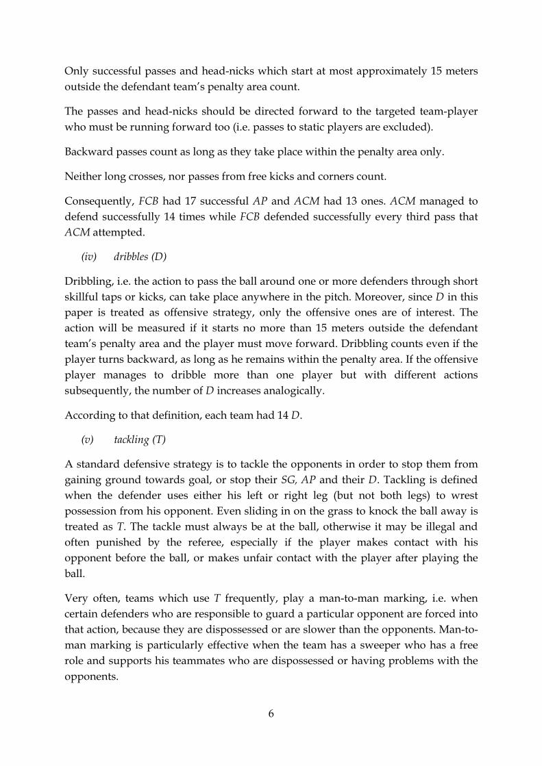
Only successful passes and head-nicks which start at most approximately 15 meters

outside the defendant team’s penalty area count.

The passes and head-nicks should be directed forward to the targeted team-player

who must be running forward too (i.e. passes to static players are excluded).

Backward passes count as long as they take place within the penalty area only.

Neither long crosses, nor passes from free kicks and corners count.

Consequently, FCB had 17 successful AP and ACM had 13 ones. ACM managed to

defend successfully 14 times while FCB defended successfully every third pass that

ACM attempted.

(iv) dribbles (D)

Dribbling, i.e. the action to pass the ball around one or more defenders through short

skillful taps or kicks, can take place anywhere in the pitch. Moreover, since D in this

paper is treated as offensive strategy, only the offensive ones are of interest. The

action will be measured if it starts no more than 15 meters outside the defendant

team’s penalty area and the player must move forward. Dribbling counts even if the

player turns backward, as long as he remains within the penalty area. If the offensive

player manages to dribble more than one player but with different actions

subsequently, the number of D increases analogically.

According to that definition, each team had 14 D.

(v) tackling (T)

A standard defensive strategy is to tackle the opponents in order to stop them from

gaining ground towards goal, or stop their SG, AP and their D. Tackling is defined

when the defender uses either his left or right leg (but not both legs) to wrest

possession from his opponent. Even sliding in on the grass to knock the ball away is

treated as T. The tackle must always be at the ball, otherwise it may be illegal and

often punished by the referee, especially if the player makes contact with his

opponent before the ball, or makes unfair contact with the player after playing the

ball.

Very often, teams which use T frequently, play a man-to-man marking, i.e. when

certain defenders who are responsible to guard a particular opponent are forced into

that action, because they are dispossessed or are slower than the opponents. Man-to-

man marking is particularly effective when the team has a sweeper who has a free

role and supports his teammates who are dispossessed or having problems with the

opponents.

7

Only T at less than approximately 15 meters outside the defendant team’s penalty

area is counted. Tackling (and head-nicks as well) from free kicks and corners are

also counted, because in these cases, the defenders play the man-to-man tactic. On

the other hand, SG, CA, AP and D stopped by unjust T and punished by the referee,

does not count.

According to these criteria, FCB defenders had 6 successful T against SG, 8 against

CA, 6 against AP and 8 against D. Similarly ACM had, 4, 9, 8 and 7 successful T

respectively.

(vi) zone marking (ZM)

In ZM every defender and the defensive midfielders too, are responsible to cover a

particular zone on the pitch to hinder the opponent players from SG, AP, D or CA

into their area. In a perfect ZM, there are two lines of defenders, usually with four

players in the first and at least three in the second line, covering roughly the one half

of the pitch. A successful ZM requires that every defender fulfills his duties,

communicates with his teammates, covers all empty spaces and synchronizes his

movement. In that case, the defensive line can exploit the offside rules and prevent

the success of long-balls, CA, AP, D and SG. Bad communication from the defenders

though can be very decisive, especially if the opponents have very quick attackers

who can dribble, pass and shot equally well.

Since measuring ZM is very difficult, the following conditions are applied to simplify

that tactic.

The two lines of defenders should be placed at about less than 10 and 20 meters

respectively, outside the defendant team’s penalty area, i.e. ZM near the middle of

the pitch does not count. (Normally, ZM near the middle of the pitch is observed

when the team controls the ball through passes or when it attacks).

To differentiate the ZM from the T, the own defender(s) should be at least 4-5 meters

away from their offensive player(s) when he (they) intercepted the ball.

Despite the fact that offside positions are the result of a good ZM, do not count.

Precisely as in T, unjust actions by ZM do not count.

According to these conditions, FCB defenders had 5 successful ZM against SG, 6

against CA, 7 against AP and 10 against D. Similarly ACM had, 9, 7, 6 and 10

successful ZM respectively.

The payoff of the game for all six strategies is depicted in the Table 1 below. Notice

that some entries are empty because both teams can’t play simultaneously offensive

or defensive. When one team attacks (defends) the other team will defend (attack).

8

The first entry refers to FCB and the second entry to ACM. Consequently, since the

payoff from a team’s offensive strategy is not equal to the negative payoff from the

other team’s defensive strategy, the game is a non-zero sum and the payoff matrix is

bi-matrix.

Table 1: The payoff matrix

a1 = SG; a2 = CA; a3 = AP; a4 = D; a5 = T; a6 = ZM; b1 = SG; b2 = CA; b3 = AP; b4 = D; b5 = T; b6 =

ZM

There seem to be some doubtful pairs, where the defensive values are higher than the

offensive ones, such as (a4, b6). How can 8 D be defended by 10 ZM? Simply, some D

which counts was defended occasionally by a ZM which also counts; the ball is then

lost to the offensive player who tried to dribble again, but failed. Consequently, the

new D attempt does not count while the new ZM does.

Notice also that there are no pure dominant strategies. But, despite the fact that there

are no pure dominant strategies, FCB gets more points than ACM from the match.

For instance, FCB had 17 AP, (a3), in comparison with ACM which had only 13, (b3).

As a whole, FCB beats ACM in six offensive-defensive pairs by a total of 11 points, is

beaten by ACM in five pairs, by 8 points, while in five pairs there is a tie. The highest

differences in favor of FCB are in (a3, b5), i.e. when FCB plays its AP and ACM does

not succeed with its defensive T, and in (a5, b4), when ACM tries with its D but FCB

defends successfully with its T.

3. Models In this section I will present four deterministic models, one chance constrained, one

possibilistic and one fuzzy LP. Five of them are formulated separately for each team

and two simultaneously for both teams.

3.1 Classical Optimization

A = FC

Barcelona

(FCB)

B = AC Milan (ACM) ∑FCB

Offensive Defensive b1 b2 b3 b4 b5 b6

Offensive

a1 0 0 0 0 5, 4 9, 9 14

a2 0 0 0 0 8, 9 7, 7 15

a3 0 0 0 0 11, 8 6, 6 17

a4 0 0 0 0 6, 7 8, 10 14

Defensive a5 6, 6 8, 7 6, 8 8, 5 0 0 28

a6 5, 7 6, 6 7, 5 10, 9 0 0 28

∑ACM 13 13 13 14 28 32

9

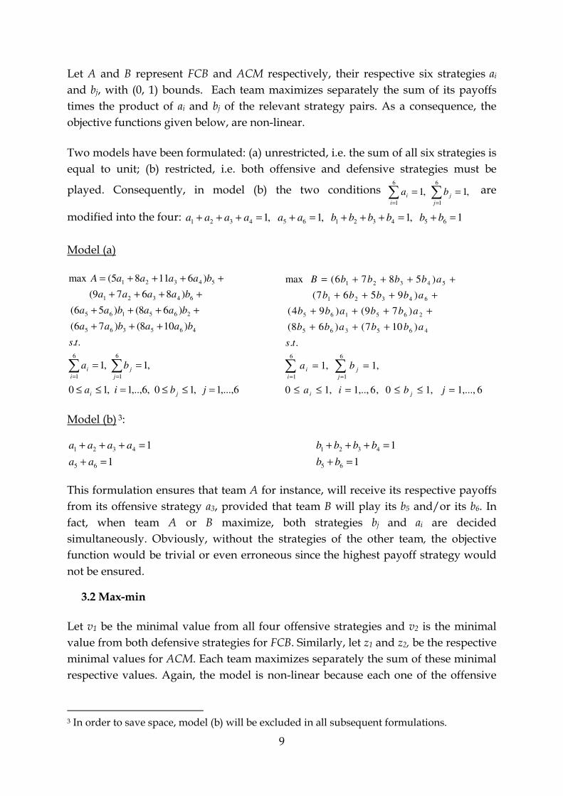
Let A and B represent FCB and ACM respectively, their respective six strategies ai

and bj, with (0, 1) bounds. Each team maximizes separately the sum of its payoffs

times the product of ai and bj of the relevant strategy pairs. As a consequence, the

objective functions given below, are non-linear.

Two models have been formulated: (a) unrestricted, i.e. the sum of all six strategies is

equal to unit; (b) restricted, i.e. both offensive and defensive strategies must be

played. Consequently, in model (b) the two conditions ,1,16

1

6

1

== ∑∑== j

j

i

i ba are

modified into the four: 1,1,1,1 654321654321 =+=+++=+=+++ bbbbbbaaaaaa

Model (a)

6,...,1,10,6,..,1,10

,1,1

..

)108()76(

)68()56(

)8679(

)61185(max

6

1

6

1

465365

265165

64321

54321

=≤≤=≤≤

==

+++

++++

++++

++++=

∑∑==

jbia

ba

ts

baabaa

baabaa

baaaa

baaaaA

ji

j

j

i

i

6,...,1,10,6,..,1,10

,1,1

..

)107()68(

)79()94(

)9567(

)5876(max

6

1

6

1

465365

265165

64321

54321

=≤≤=≤≤

==

+++

++++

++++

++++=

∑∑==

jbia

ba

ts

abbabb

abbabb

abbbb

abbbbB

ji

j

j

i

i

Model (b) 3:

11

11

6565

43214321

=+=+

=+++=+++

bbaa

bbbbaaaa

This formulation ensures that team A for instance, will receive its respective payoffs

from its offensive strategy a3, provided that team B will play its b5 and/or its b6. In

fact, when team A or B maximize, both strategies bj and ai are decided

simultaneously. Obviously, without the strategies of the other team, the objective

function would be trivial or even erroneous since the highest payoff strategy would

not be ensured.

3.2 Max-min

Let v1 be the minimal value from all four offensive strategies and v2 is the minimal

value from both defensive strategies for FCB. Similarly, let z1 and z2, be the respective

minimal values for ACM. Each team maximizes separately the sum of these minimal

respective values. Again, the model is non-linear because each one of the offensive

3 In order to save space, model (b) will be excluded in all subsequent formulations.

10

(defensive) strategies of one team is multiplied by the defensive (offensive) strategies

of the other team.

Model (a)

6,...,1,10,6,..,1,10

,1,1

)108(

)76(

)68(

)56(

)8679(

)61185(..

max

6

1

6

1

2465

2365

2265

2165

164321

154321

21

=≤≤=≤≤

==

≥+

≥+

≥+

≥+

≥+++

≥+++

+=

∑∑==

jbia

ba

vbaa

vbaa

vbaa

vbaa

vbaaaa

vbaaaats

vvA

ji

j

j

i

i

6,...,1,10,6,..,1,10

,1,1

)107(

)68(

)79(

)94(

)9567(

)5876(..

max

6

1

6

1

2465

2365

2265

2165

164321

154321

21

=≤≤=≤≤

==

≥+

≥+

≥+

≥+

≥+++

≥+++

+=

∑∑==

jbia

ba

zabb

zabb

zabb

zabb

zabbbb

zabbbbts

zzB

ji

j

j

i

i

3.3 LP formulation with complementary conditions

While the first two models assume that teams optimize separately, we turn now to a

simultaneously optimal decisions. Normally, for a bimatrix game with many

strategies, it is rather difficult to find a solution that is simultaneously optimal for

both teams. We can define an equilibrium stable set of strategies though, i.e. the well

known Nash equilibrium. In the following two sections I will formulate two models

to find the Nash equilibrium.

As is known, the max-min strategy is defined as:

���� , . . , ���� �� max���,..,��� min���,..,��� ������� ����, . . , ���, ���, . . , ���� ����, . . , ���� �� max���,..,��� min���,..,��� ������� ����, . . , ���, ���, . . , ���� A standard model to find a max-min to both teams is to use a simultaneous LP, with

complementary conditions. The complementary conditions are to set the product of

each one of the six respective slack, times the six respective strategies, equal to zero.

According to this formulation, both teams behave symmetrically, since they

maximize their own minimal payoffs obtained from their own selected strategies.

Compared to the previous models, each team selects now only its own strategies.

Notice also the two extra constraints, which ensure that both teams can’t play

entirely offensively or defensively4. For instance, the upper bound for all offensive

4 Without these additional constraints, both teams played offensively; FCB plays 55.55% SG and 44.45% AP, while ACM plays 57.14% AP and 42.86% D.

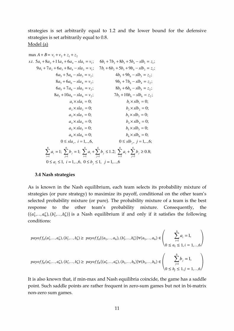
11

strategies is set arbitrarily equal to 1.2 and the lower bound for the defensive

strategies is set arbitrarily equal to 0.8.

Model (a)

6,...,1,10,6,..,1,10

;8.0;2.1;1;1

;6,..,1,0,6,..,1,0

;0;0

;0;0

;0;0

;0;0

;0;0

;0;0

;107;108

;68;76

;79;68

;94;56

;9567;8679

;5876;61185..

max

6

5

6

5

4

1

4

1

6

1

6

1

6666

5555

4444

3333

2222

1111

26652665

25652565

24652465

23652365

124321124321

114321114321

2121

=≤≤=≤≤

≥+≤+==

=≤=≤

=×=×

=×=×

=×=×

=×=×

=×=×

=×=×

=−+=−+

=−+=−+

=−+=−+

=−+=−+

=−+++=−+++

=−+++=−+++

+++=+

∑∑∑∑∑∑======

jbia

bababa

jslbisla

slbbslaa

slbbslaa

slbbslaa

slbbslaa

slbbslaa

slbbslaa

zslbbbvslaaa

zslbbbvslaaa

zslbbbvslaaa

zslbbbvslaaa

zslbbbbbvslaaaaa

zslbbbbbvslaaaaats

zzvvBA

ji

j

j

i

i

j

j

i

i

j

j

i

i

ji

3.4 Nash strategies

As is known in the Nash equilibrium, each team selects its probability mixture of

strategies (or pure strategy) to maximize its payoff, conditional on the other team’s

selected probability mixture (or pure). The probability mixture of a team is the best

response to the other team’s probability mixture. Consequently, the ����� , . . , ����, ����, . . , ����� is a Nash equilibrium if and only if it satisfies the following

conditions:

�����������, . . , ��� �, ����, . . , ���� � �����������, . . , ���, ����, . . , ����� ���, . . , ��� ! " ,16

1

=∑=i

ia

0 $ �% $ 1, ' 1, . . ,6)

�����������, . . , ����, ����, . . , ���� � ������������, . . , ��� �, ���, . . , ���� ���, . . , ��� ! *+ ,1

6

1

=∑=j

jb

0 $ �, $ 1, - 1, . . ,6./

It is also known that, if min-max and Nash equilibria coincide, the game has a saddle

point. Such saddle points are rather frequent in zero-sum games but not in bi-matrix

non-zero sum games.

12

I appied the package by Dickhaut & Kaplan (1993) programmed in Mathematica, to

find the Nash equilibria. In model (a) the entire payoff matrix was used. In model (b)

I used two sub-matrices; when FCB (ACM) was playing offensively and ACM (FCB)

defensively.

3.5 Chance-Constrained Programming (CCP)

When teams are uncertain about competitors’ actions or about the payoff matrix,

games become very complex. According to Carlton & Perloff (2005) much of the

current research in game theory is undertaken on games with uncertainty. I move

now to some more plausible models and modify the deterministic parameters and

constraints.

In CCP the parameters of the constraints are random variables and the constraints

are valid with some (minimum) probability.

Let us assume that the deterministic parameters are expected values, independent

and normally distributed random variables with the means as previously, and

variances5 given in Table 2. The first entry depicts the variance for FCB and the

second for ACM.

Table 2: The variance of the payoff matrix

Moreover, in CCP, when we maximize for one team, we assume that the other team’s

values are deterministic and disregard their variance. We also assume that, Josep

Guardiola, the manager of FCB, might expect that the probability of the expected

value of his team’s defensive strategies a5 and a6 is at least 90%, while the probability

of all four expected values of offensive strategies, a1, a2, a3 and a4 is at least 95%.

5 The variances of the payoffs are obviously very subjective and are given just to show the formulation of the model. Moreover, based on my numerous playing back of the match, the variances reflect rather well the uncertainty of the respective payoffs.

A = FC Barcelona (FCB)

B = AC Milan (ACM)

Offensive Defensive

1

2bσ 2

2bσ

3

2bσ

4

2bσ 5

2bσ 6

2bσ

Offensive

1

2aσ 0 0 0 0 9, 10 17, 12

2

2aσ 0 0 0 0 16, 15 15, 13

3

2aσ 0 0 0 0 17, 14 10, 11

4

2aσ 0 0 0 0 13, 13 15, 14

Defensive

5

2aσ 10, 9 12, 11 15, 15 11, 12 0 0

6

2aσ 10, 12 11, 10 14, 13 16, 16 0 0

13

The first stochastic constraint is now formulated as:

{ }

+++

+++−=−≥+++≤

2

4

2

3

2

2

2

1

543211543211

1317169

)61185(1)61185(

aaaa

baaaavFbaaaavP α ,

where, F is the cumulative density function of the standard normal distribution. If F

(K5) is the standard normal value such that F (K5) = 1 - 5, then the above constraint

reduces to: ( )αKaaaa

baaaav≥

+++

+++−2

4

2

3

2

2

2

1

543211

1317169

)61185(

Given 10.0=α , the constraint is simplified to:

1

2

4

2

3

2

2

2

154321 1317169282.1)61185( vaaaabaaaa ≥+++++++

Similarly, given 05.0=α , the first defensive constraint is modified to:

2

2

6

2

5165 1010645.1)56( vaabaa ≥+++

So, the CCP model (a) for FCB is:

6,...,1,10,6,..,1,10

,1,1

1611645.1)108(

1415645.1)76(

1112645.1)68(

1010645.1)56(

15101517282.1)8679(

1317169282.1)61185(..

max

6

1

6

1

2

2

6

2

5465

2

2

6

2

5365

2

2

6

2

5265

2

2

6

2

5165

1

2

4

2

3

2

2

2

164321

1

2

4

2

3

2

2

2

154321

21

=≤≤=≤≤

==

≥+++

≥+++

≥+++

≥+++

≥+++++++

≥+++++++

+=

∑∑==

jbia

ba

vaabaa

vaabaa

vaabaa

vaabaa

vaaaabaaaa

vaaaabaaaats

vvA

ji

j

j

i

i

A similar formulation applies for ACM, assuming that its manager Massimiliano

Allegri expects that the probability of the expected value of his team’s defensive

strategies b5 and b6 is also at least 90%, while the probability of all four offensive

strategies, b1, b2, b3 and b4 is at least 95%. Allegri also treats Barcelona’s values as

deterministic and therefore the problem is formulated similarly.

3.6 A Possibilistic LP (PLP) model

No matter how well one has defined and measured the six variables, the observed

payoffs are still rather ambiguous.

14

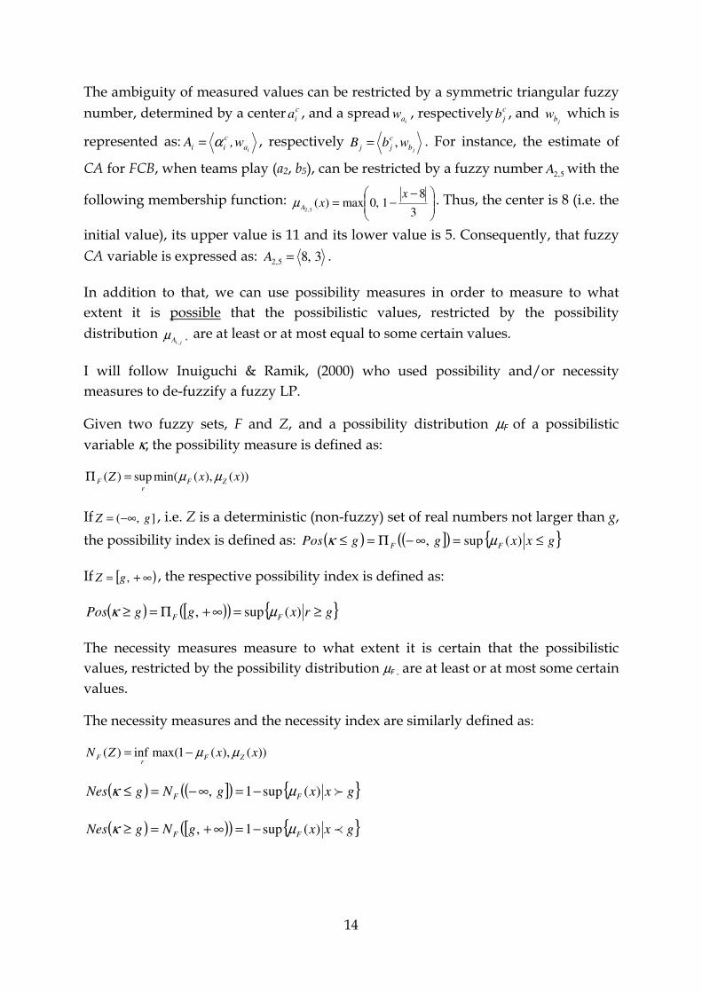
The ambiguity of measured values can be restricted by a symmetric triangular fuzzy

number, determined by a center c

ia , and a spreadiaw , respectively c

jb , and jbw which is

represented as:ia

c

ii w,A α= , respectively jb

c

jj wbB ,= . For instance, the estimate of

CA for FCB, when teams play (a2, b5), can be restricted by a fuzzy number5,2A with the

following membership function:

−−=

3

81,0max)(

5,2

xxAµ . Thus, the center is 8 (i.e. the

initial value), its upper value is 11 and its lower value is 5. Consequently, that fuzzy

CA variable is expressed as: 3,85,2 =A .

In addition to that, we can use possibility measures in order to measure to what

extent it is possible that the possibilistic values, restricted by the possibility

distribution jiA ,

µ , are at least or at most equal to some certain values.

I will follow Inuiguchi & Ramik, (2000) who used possibility and/or necessity

measures to de-fuzzify a fuzzy LP.

Given two fuzzy sets, F and Z, and a possibility distribution µF of a possibilistic

variable κ, the possibility measure is defined as:

))(),(min(sup)( xxZ ZFr

F µµ=Π

If ],( gZ −∞= , i.e. Z is a deterministic (non-fuzzy) set of real numbers not larger than g,

the possibility index is defined as: ( ) ( ]( ) { }gxxggPos FF ≤=∞−Π=≤ )(sup, µκ

If [ )∞+= ,gZ , the respective possibility index is defined as:

( ) [ )( ) { }grxggPos FF ≥=∞+Π=≥ )(sup, µκ

The necessity measures measure to what extent it is certain that the possibilistic

values, restricted by the possibility distribution µF , are at least or at most some certain

values.

The necessity measures and the necessity index are similarly defined as:

))(),(1max(inf)( xxZN ZFr

F µµ−=

( ) ( ]( ) { }gxxgNgNes FF f)(sup1, µκ −=∞−=≤

( ) [ )( ) { }gxxgNgNes FF p)(sup1, µκ −=∞+=≥

15

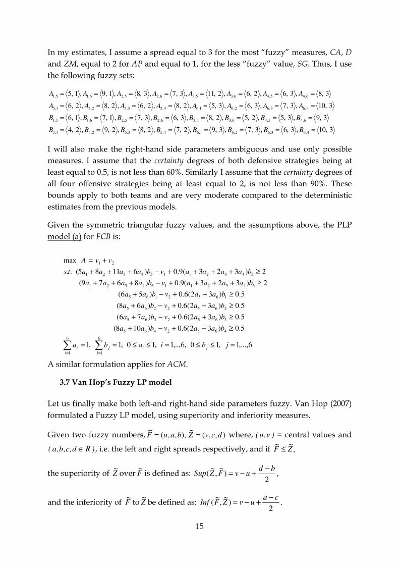
In my estimates, I assume a spread equal to 3 for the most “fuzzy” measures, CA, D

and ZM, equal to 2 for AP and equal to 1, for the less “fuzzy” value, SG. Thus, I use

the following fuzzy sets:

3,10,3,6,3,7,3,9,2,7,2,8,2,9,2,4

3,9,3,5,2,5,2,8,3,6,3,7,1,7,1,6

3,10,3,7,3,6,3,5,2,8,2,6,2,8,2,6

3,8,3,6,2,6,2,11,3,7,3,8,1,9,1,5

4,63,62,61,64,53,52,51,5

6,45,46,35,36,25,26,15,1

4,63,62,61,64,53,52,51,5

6,45,46,35,36,25,26,15,1

========

========

========

========

BBBBBBBB

BBBBBBBB

AAAAAAAA

AAAAAAAA

I will also make the right-hand side parameters ambiguous and use only possible

measures. I assume that the certainty degrees of both defensive strategies being at

least equal to 0.5, is not less than 60%. Similarly I assume that the certainty degrees of

all four offensive strategies being at least equal to 2, is not less than 90%. These

bounds apply to both teams and are very moderate compared to the deterministic

estimates from the previous models.

Given the symmetric triangular fuzzy values, and the assumptions above, the PLP

model (a) for FCB is:

A similar formulation applies for ACM.

3.7 Van Hop’s Fuzzy LP model

Let us finally make both left-and right-hand side parameters fuzzy. Van Hop (2007)

formulated a Fuzzy LP model, using superiority and inferiority measures.

Given two fuzzy numbers, ),,(~

),,,(~

dcvZbauF == where, )v,u( = central values and

)Rd,c,b,a( ∈ , i.e. the left and right spreads respectively, and if ,~~ZF ≤

the superiority of Z~overF

~is defined as:

2)

~,

~(

bduvFZSup

−+−= ,

and the inferiority of F~to Z

~be defined as:

2)

~,

~(

cauvZFInf

−+−= .

6,...,1,10,6,..,1,10,1,1

5.0)32(6.0)108(

5.0)32(6.0)76(

5.0)32(6.0)68(

5.0)32(6.0)56(

2)323(9.0)8679(

2)323(9.0)61185(..

max

6

1

6

1

4652465

3652365

2652265

1652165

64321164321

54321154321

21

=≤≤=≤≤==

≥++−+

≥++−+

≥++−+

≥++−+

≥++++−+++

≥++++−+++

+=

∑∑==

jbiaba

baavbaa

baavbaa

baavbaa

baavbaa

baaaavbaaaa

baaaavbaaaats

vvA

ji

j

j

i

i

16

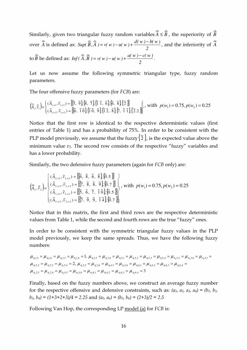
Similarly, given two triangular fuzzy random variables B~

A~

≤ , the superiority of B~

over A~is defined as:

2

)w(b)w(d)w(u)w(v)A

~,B

~(Sup

−+−= , and the inferiority of A

~

toB~be defined as:

2

)w(c)w(a)w(u)w(v)B

~,A

~(Inf

−+−= .

Let us now assume the following symmetric triangular type, fuzzy random

parameters.

The four offensive fuzzy parameters (for FCB) are:

( ) { }{ }{ }{ }{ }[ ]{ }{ }{ }{ }{ }[ ]

=

==

2.2~

,1~

1~

,7,8~

,2~

1~

,9~

,0~

1~

,0~

1~

,6~

)~,~

(

2~

,8~

,6~

,6~

,1~

1~

,7~

,8~

,9~

,5~

)~,~

(~,

~

2,12,1

1,11,1

11

ww

ww

vA

vAvA , with 25.0)(,75.0)( 21 == wpwp

Notice that the first row is identical to the respective deterministic values (first

entries of Table 1) and has a probability of 75%. In order to be consistent with the

PLP model previously, we assume that the fuzzy{ }2~

, is the expected value above the

minimum value v1. The second row consists of the respective “fuzzy” variables and

has a lower probability.

Similarly, the two defensive fuzzy parameters (again for FCB only) are:

( )

{ }{ }[ ]{ }{ }[ ]{ }{ }[ ]{ }{ }[ ]

=

=

=

=

=

7.0~

,4~

1~

,9~

,9~

,7~

)~,~

(

5.0~

,0~

1~

,7~

,6~

,5~

)~,~

(

7.0~

,9~

,8~

,8~

,7~

)~,~

(

5.0~

,8~

,6~

,8~

,6~

)~,~

(

~,

~

2,22,2

1,21,2

2,22,2

1,21,2

22

ww

ww

ww

ww

vA

vA

vA

vA

vA, with 25.0)(,75.0)( 21 == wpwp

Notice that in this matrix, the first and third rows are the respective deterministic

values from Table 1, while the second and fourth rows are the true “fuzzy” ones.

In order to be consistent with the symmetric triangular fuzzy values in the PLP

model previously, we keep the same spreads. Thus, we have the following fuzzy

numbers:

3

,2

,1

4,63,62,61,66,45,46,25,2

4,63,62,61,66,45,46,25,24,53,52,5

1,56,35,34,53,52,51,56,35,36,15,16,15,1

22222222

11111111222

2221111112211

========

===========

=============

AAAAAAAA

AAAAAAAAAAA

AAAAAAAAAAAAA

µµµµµµµµ

µµµµµµµµµµµ

µµµµµµµµµµµµµ

Finally, based on the fuzzy numbers above, we construct an average fuzzy number

for the respective offensive and defensive constraints, such as: (a1, a2, a3, a4) = (b1, b2,

b3, b4) = (1+3+2+3)/4 = 2.25 and (a5, a6) = (b5, b6) = (2+3)/2 = 2.5

Following Van Hop, the corresponding LP model (a) for FCB is:

17

4,..,1,6,5,0

6,..,1,10,6,..,1,10,1,1

2

)32(5.27.0)149(

2

)32(5.27.0)98(

2

)32(5.27.0)98(

2

)32(5.27.0)77(

2

5.2)32(5.0)108(

2

5.2)32(5.0)76(

2

5.2)32(5.0)68(

2

5.2)32(5.0)56(

2

)323(25.22.2)118910(

2

)323(25.22.2)712106(

2

25.2)323(2)8679(

2

25.2)323(2)61185(..

25.075.0max

inf

2

inf

1

sup

2

sup

1

6

1

6

1

inf

24465

2465

inf

23365

2365

inf

22265

2265

inf

21165

2165

sup

24465

2465

sup

23365

2365

sup

22265

2265

sup

21165

2165

inf

1664321

164321

inf

1554321

154321

sup

1664321

164321

sup

1554321

154321

4

1

inf

2

6

5

inf

1

4

1

sup

2

6

5

sup

121

==≥===

=≤≤=≤≤==

=+−

++−+

=+−

++−+

=+−

++−+

=+−

++−+

=−+

++−+

=−+

++−+

=−+

++−+

=−+

++−+

=+++−

++−+++

=+++−

++−+++

=−+++

++−+++

=−+++

++−+++

+−

+−+=

∑∑

∑∑∑∑

==

====

mk

jbiaba

baavbaa

baavbaa

baavbaa

baavbaa

baavbaa

baavbaa

baavbaa

baavbaa

baaaavbaaaa

baaaavbaaaa

baaaavbaaaa

baaaavbaaaats

vvA

mkmk

ji

j

j

i

i

m

m

k

k

m

m

k

k

λλλλ

λ

λ

λ

λ

λ

λ

λ

λ

λ

λ

λ

λ

λλλλ

A similar formulation applies for ACM.

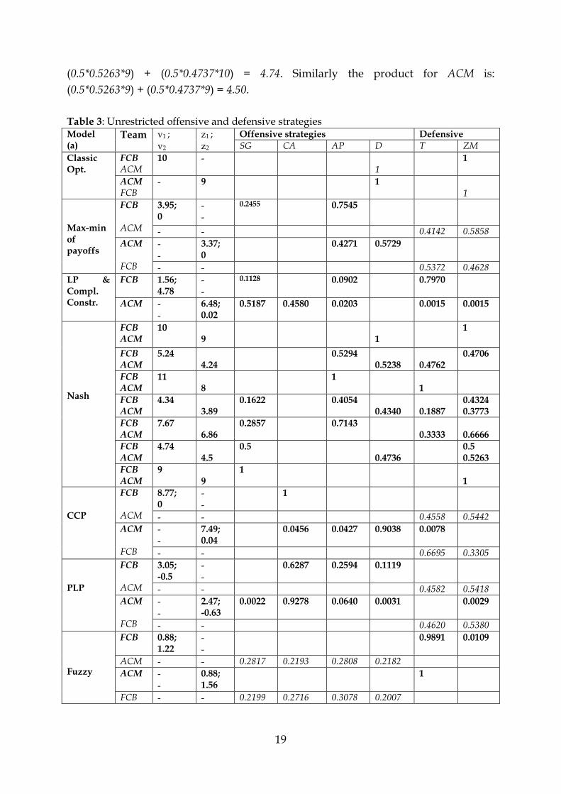
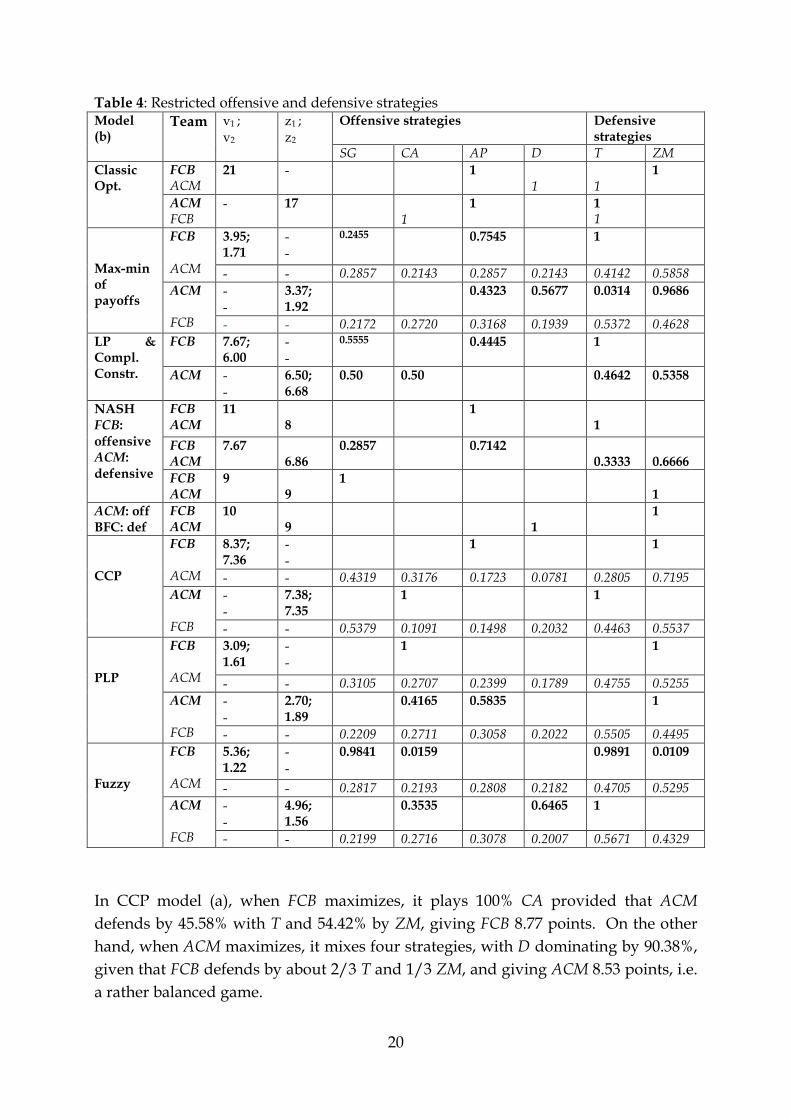
4. Results

The unrestricted offensive and defensive strategies, model (a), are presented in Table

3 and the restricted ones, model (b), are presented in Table 4. The maximizing team is

in bald and the other team in italics. In LP with complementary constraints and in the

Nash, both teams maximize and are in bald.

In classical optimization model (a), both teams play pure strategies, FCB receives 10

points and ACM 9. It is rather surprising because FCB plays defensively and ACM

plays offensively, no matter which team maximizes. In both cases, FCB plays ZM and

ACM plays D, (a6 = b4 = 1).

In model (b), the strategies change. When FCB maximizes, it plays the pure strategies

AP and ZM (a3 = a6 = 1) and receives 21, under the condition that ACM plays also its

18

pure strategies T and D, (b5 = b4 = 1). When ACM maximizes, it receives 17, by

playing AP and T, (b3 = b5 = 1), given that FCB plays T and CA, (a5 = a2 = 1)6.

In the maximization of the minimum payoffs, model (a), both teams use mixed

offensive strategies when they maximize separately. When FCB maximizes, it gets

3.95 points, if it plays offensively (75.45% AP and 24.55% SG) and ACM plays

defensively (58.58% ZM and 41.42% T). Similarly, when ACM maximizes, it gets 3.37

points when it also plays offensively (42.71% AP and 57.29% D) and FCB plays

defensively (46.28% ZM and 53.72% T).

In model (b), when FCB maximizes, it continues with the same offensive game but it

plays 100% T as well. Given the fact that ACM continues with the same defensive

game and almost equally balanced with all the offensive strategies, FCB gets 3.95 +

1.71 = 5.66 points. When ACM maximizes, it continues with almost the same weights

in AP and D, and also plays almost 97% ZM and 3% T. Since FCB continues with the

same mixture in defense, and also with all four offensive ones, with AP just above

30%, ACM gets 3.37 + 1.92 = 5.29 points.

In the LP with complementary constraints model (a), FCB plays mainly defensively

(almost 80% T) and ACM almost offensively (51.87% SG and 45.8% CA), with two

positive slacks (sla4 = 1.59, sla6 = 1.59), giving ACM more points than FCB!

In model (b), FCB mixes two offensive strategies (55.55% SG and 44.45% AP) and

plays also 100% T. ACM shifts strategies by playing 50% SG and 50% CA, and also

mixing its defensive strategies, with more weights in ZM. FCB gets more points from

its offensive strategies (v1 = 7.67, v2 = 6), while ACM gets slightly more points from its

defensive strategies (z1 = 6.5, z2 = 6.68). Notice though that in this case there are five

positive slacks, sla4 = 2, sla6 = 2, slb4 = 1.25, slb5 = 0.25, slb6 = 1.93.

In Nash, model (a), Mathematica found seven equilibria, with three of them being

pure strategies and four mixed ones. The three pure strategies and one of the four

mixed ones are identical in model (b) as well. Notice also that the pure strategies

Nash equilibrium (a6 = b4 = 1) is identical with the solution from the classical

optimization when FCB maximizes and is the only one where ACM plays offensively.

Apart from the Nash payoff (9, 9), in all other equilibria FCB gets more points than

ACM, with the largest difference (11, 8) when FCB plays 100% AP and ACM defends

with 100% T. In another Nash equilibrium, (4.74, 4.5), the difference is approximately

5% in favor of FCB. That equilibrium is found if FCB plays 50% its a1 and 50% its a6,

while ACM plays 52.63% its b6 and 47.37% its b4. In that case the product for FCB is:

6 Notice that ACM would also receive 17 points too if it accepted the solution in which FCB maximizes, i.e. (a3 = a6 = 1) and (b5 = b4 = 1).

19

(0.5*0.5263*9) + (0.5*0.4737*10) = 4.74. Similarly the product for ACM is:

(0.5*0.5263*9) + (0.5*0.4737*9) = 4.50.

Table 3: Unrestricted offensive and defensive strategies Model (a)

Team v1 ; v2

z1 ; z2

Offensive strategies Defensive SG CA AP D T ZM

Classic Opt.

FCB ACM

10 - 1

1

ACM FCB

- 9 1 1

Max-min of payoffs

FCB

ACM

3.95; 0

- -

0.2455 0.7545

- - 0.4142 0.5858

ACM FCB

- -

3.37; 0

0.4271 0.5729

- - 0.5372 0.4628

LP & Compl. Constr.

FCB 1.56; 4.78

- -

0.1128 0.0902 0.7970

ACM - -

6.48; 0.02

0.5187 0.4580 0.0203 0.0015 0.0015

Nash

FCB ACM

10 9

1

1

FCB ACM

5.24 4.24

0.5294 0.5238

0.4762

0.4706

FCB ACM

11 8

1 1

FCB ACM

4.34 3.89

0.1622 0.4054 0.4340

0.1887

0.4324 0.3773

FCB ACM

7.67 6.86

0.2857 0.7143 0.3333

0.6666

FCB ACM

4.74 4.5

0.5 0.4736

0.5 0.5263

FCB ACM

9 9

1 1

CCP

FCB ACM

8.77; 0

- -

1

- - 0.4558 0.5442

ACM FCB

- -

7.49; 0.04

0.0456 0.0427 0.9038

0.0078

- - 0.6695 0.3305

PLP

FCB ACM

3.05; -0.5

- -

0.6287 0.2594 0.1119

- - 0.4582 0.5418

ACM FCB

- -

2.47; -0.63

0.0022 0.9278 0.0640 0.0031 0.0029

- - 0.4620 0.5380

Fuzzy

FCB

0.88; 1.22

- -

0.9891 0.0109

ACM - - 0.2817 0.2193 0.2808 0.2182

ACM

- -

0.88; 1.56

1

FCB - - 0.2199 0.2716 0.3078 0.2007

20

Table 4: Restricted offensive and defensive strategies Model (b)

Team v1 ; v2

z1 ; z2

Offensive strategies Defensive strategies

SG CA AP D T ZM

Classic Opt.

FCB ACM

21 - 1 1

1

1

ACM FCB

- 17 1

1 1 1

Max-min of payoffs

FCB ACM

3.95; 1.71

- -

0.2455 0.7545 1

- - 0.2857 0.2143 0.2857 0.2143 0.4142 0.5858

ACM FCB

- -

3.37; 1.92

0.4323 0.5677 0.0314 0.9686

- - 0.2172 0.2720 0.3168 0.1939 0.5372 0.4628

LP & Compl. Constr.

FCB 7.67; 6.00

- -

0.5555 0.4445 1

ACM - -

6.50; 6.68

0.50 0.50 0.4642 0.5358

NASH FCB: offensive ACM: defensive

FCB ACM

11 8

1 1

FCB ACM

7.67 6.86

0.2857 0.7142

0.3333

0.6666

FCB ACM

9 9

1

1

ACM: off BFC: def

FCB ACM

10 9

1

1

CCP

FCB ACM

8.37; 7.36

- -

1

1

- - 0.4319 0.3176 0.1723 0.0781 0.2805 0.7195

ACM FCB

- -

7.38; 7.35

1 1

- - 0.5379 0.1091 0.1498 0.2032 0.4463 0.5537

PLP

FCB ACM

3.09; 1.61

- -

1 1

- - 0.3105 0.2707 0.2399 0.1789 0.4755 0.5255

ACM FCB

- -

2.70; 1.89

0.4165 0.5835 1

- - 0.2209 0.2711 0.3058 0.2022 0.5505 0.4495

Fuzzy

FCB ACM

5.36; 1.22

- -

0.9841 0.0159 0.9891 0.0109

- - 0.2817 0.2193 0.2808 0.2182 0.4705 0.5295

ACM FCB

- -

4.96; 1.56

0.3535 0.6465 1

- - 0.2199 0.2716 0.3078 0.2007 0.5671 0.4329

In CCP model (a), when FCB maximizes, it plays 100% CA provided that ACM

defends by 45.58% with T and 54.42% by ZM, giving FCB 8.77 points. On the other

hand, when ACM maximizes, it mixes four strategies, with D dominating by 90.38%,

given that FCB defends by about 2/3 T and 1/3 ZM, and giving ACM 8.53 points, i.e.

a rather balanced game.

21

In model (b), both teams shift strategies. When FCB maximizes, it plays 100% AP and

100% ZM, while ACM plays all six strategies with changes in defense weights. When

ACM maximizes, it shifts to two pure strategies, 100% CA and 100% T, while FCB

plays all six strategies too and changes also its defense weights. In this model, the

offensive strategies give 8.37 points to FCB and 7.38 points to ACM. On the other

hand, both teams get almost the same points (7.36 versus 7.35) from their defensive

strategies.

In PLP model (a), the results are rather similar as in CCP. Both teams, when they

maximize, mix their offensive strategies, with most weights in CA. Both teams mix

also their defensive strategies (with almost identical weights) when the other team

maximizes. FCB gets 3.05 and ACM 2.47 points. Notice though the two negative

values in the defensive strategies, v2 = - 0.5 and z2 = - 0.63, indicating that the

certainty degree of defensive strategies being at least equal to 0.5, should not be less

than 60%, is violated. For ACM, the additional - 0.13 is explained by the fact that b6 =

0.0029. On the other hand, the certainty degrees of all four offensive strategies being

at least equal to 2, should not be less than 90%, is valid.

In PLP, model (b), both certainty degrees are satisfied. Both teams, when they

maximize, play 100% ZM, FCB plays also 100% CA, while ACM mixes its CA with

AP. When one team maximizes, the other team mixes all six strategies, with roughly

similar weights. FCB gets 3.09 + 1.61 = 4.7 points, while ACM gets 2.70 + 1.89 = 4.59

points, again a rather balanced game.

Finally, in Fuzzy model (a), both teams, play similar strategies when they maximize,

100% T for ACM and almost 99% for FCB, and mix all four offensive strategies, with

almost similar weights, when the other team maximizes. They get the same points

from their offensive strategies, but ACM gets more points than BFC from its pure

defensive strategy T.

In Fuzzy, model (b), while the strategies from model (a) remain unchanged, FCB

plays 98.4% SG, 1.6% CA and ACM mixes about 1/3 CA and 2/3 D. Both teams mix

also their defensive strategies when the other team maximizes. Again ACM gets 0.34

more points from its T, while FCB gets 0.40 more points from its offensive strategies,

leading to almost balanced game.

Notice that in all fuzzy models all inferior lambdas are positive, varying between

1.52 and 2.9.

In general, the “average” strategies from all models (a) are: FCB plays about 57%

offensively, i.e. about 23% AP, 19% SG and 14% CA. Its highest weight though is in

22

defense, ZM with about 28%. ACM plays more offensively, 61.8%, mainly through

41% D, and by about 12% CA. ACM balances its defensive strategies, by about 21%

ZM and 17% T. The closest to these averages is the Nash equilibrium that gives FCB

4.34 points and ACM 3.89 points. Similarly, the “average” strategies from all models

(b) are: FCB plays about 54.6% AP, 34.1% SG and 11.3% CA offensively and 42.7% T

and 57.3% ZM defensively; ACM plays 32.4% CA, 31.6% D, 28.8% AP and 7.2% SG

offensively and 53.7% T and 46.3% ZM defensively.

Conclusions

A number of deterministic and stochastic models where used to find out the optimal

offensive and defensive strategies that FCB and ACM could have applied during

their UEFA CL match, based on the selected match statistics. Since FCB won the

match, the question posed was if ACM could have done better by following better

strategies.

Despite the fact that the optimal strategies vary with the selected model, there are

indeed four different strategies that ACM could have selected according to the

following models: (i) in fuzzy model (a) ACM gets 16% more points than FCB, if it

plays purely defensive, i.e. 100% T; (ii) in LP with complementary constraints model

(a) ACM gets 2.5 % more points, if it plays offensively, i.e. 52% SG and 46% CA; (iii)

in one Nash equilibrium where both teams get 9 points, if it plays 100% ZM in order

to defend the 100% SG played by FCB; (iv) in fuzzy model (b) where ACM gets 1%

less points than FCB, if it plays 100% T in defense and also 35.4% CA and 64.6% D in

offense.

On the other hand, ACM does it badly with the following strategies: (i) in PLP model

(a), if it relies mainly to CA (by 93%) with almost no defense; (ii) in one Nash

equilibrium when FCB plays 100% AP and ACM 100% T; (iii) in another Nash

equilibrium when FCB plays 53% AP and 47% ZM while ACM plays 52.4% D and

47.6% T; (iv) in classical maximization model (b), if both teams play 100% AP, and

also FCB plays 100% ZM while ACM plays 100% T.

So the final suggestion to ACM is: When both teams maximize simultaneously, play

offensively, start with counter-attacks with finish with shots on goal. FCB would try

with tackling, but not with high success. On the other hand, excessive CA if it is not

followed by SG should be avoided since FCB can mix its two defensive strategies

successfully. If FCB plays mainly its amazing passing game or its SG, defend with

ZM instead of T.

I leave it open to the readers, the funs and the managers to conclude if ACM’s defeat

can be explained because it did not followed the suggested strategies above.

23

References

Carlton, D.W. & J.M. Perloff: Modern Industrial Organization, 4th ed., Pearson Addison Wesley, (2005).

Dickhaut J. & T. Kaplan: A Program for Finding Nash Equilibria, in H.R. Varian, (ed.) Economic and Financial Modeling with Mathematica, Telos, Springer-Verlag (1993).

Inuiguchi, M. and J. Ramík: Possibilistic linear programming: a brief review of fuzzy mathematical programming and a comparison with stochastic programming in portfolio selection problem, Fuzzy Sets and Systems, 111 (2000), 3-28.

Luhandjula, M.K.: Optimization under hybrid uncertainty, Fuzzy Sets and Systems 146 (2004), 187-203.

Luhandjula, M.K.: Fuzziness and randomness in an optimization framework, Fuzzy Sets and Systems 77 (1996), 291-297.

Papahristodoulou, C.: The optimal layout of football players: A case study for AC Milan, Working Paper, Munich Personal RePec Archive, (2010), downloadable at: http://mpra.ub.uni-muenchen.de/20102/1/MPRA_paper_20102.pdf

Papahristodoulou, C.: An Analysis of UEFA Champions League Match Statistics, International Journal of Applied Sports Sciences 20 (2008), 67-93.

Pollard, R. and C. Reep: Measuring the effectiveness of playing strategies at soccer,

The Statistician, 46, (1997), 541-50.

Taha, H.A.: Operations research: An Introduction, 8th ed., Pearson Prentice Hall, Upper Saddle River, NJ, (2007).

Van Hop, N.: Solving fuzzy (stochastic) linear programming problems using

superiority and inferiority measures, Information Sciences, 177 (2007), 1977-91.

Wolfram Research, Mathematica: Fuzzy Logic (2003).

http://www.talkfootball.co.uk/guides/football_tactics.html

http://sport.virgilio.it/calcio/serie-a/statistiche/index.html

http://www.uefa.com/uefachampionsleague/season=2012/statistics/index.html