Optimal filtering for linear state delay systems

International Journal of Pure and Applied Mathematics————————————————————————–Volume 10 No. 3 2004, 241-255

OPTIMAL FILTERING FOR LINEAR

SYSTEMS WITH STATE DELAY

Michael V. Basin1 §, Jesus Rodriguez-Gonzalez2

Rodolfo Martinez-Zuniga3

1,2Department of Physical and Mathematical SciencesAutonomous University of Nuevo Leon

Apartado Postal 144-F, C.P. 66450, San Nicolas de los GarzaNuevo Leon, MEXICO

1e-mail: [email protected]: [email protected]

3Department of Electrical and Mechanical EngineeringAutonomous University of Coahuila

Calle Barranquilla, S/N, Col. GuadalupeApartado Postal 189, C.P. 25750, Monclova

Coahuila, MEXICOe-mail: [email protected]

Abstract: In this paper, the optimal filtering problem for linear systemswith state delay over linear observations is treated proceeding from the generalexpression for the stochastic Ito differential of the optimal estimate and the errorvariance. As a result, the optimal estimate equation similar to the traditionalKalman-Bucy one is derived; however, it is impossible to obtain a system ofthe filtering equations, that is closed with respect to the only two variables,the optimal estimate and the error variance, as in the Kalman-Bucy filter. Theresulting system of equations for determining the error variance consists of aset of equations, whose number is specified by the ratio between the currentfiltering horizon and the delay value in the state equation and increases as thefiltering horizon tends to infinity. In the example, performance of the designed

Received: July 28, 2003 c© 2004, Academic Publications Ltd.

§Correspondence author

242 M.V. Basin, J. Rodriguez-Gonzalez, R. Martinez-Zuniga

optimal filter for linear systems with state delay is verified against the bestKalman-Bucy filter available for linear systems without delays.

AMS Subject Classification: 60G35, 93C05, 93E11Key Words: linear time-delay system, stochastic system, filtering

1. Introduction

The optimal filtering problem for linear system states and observations withoutdelays was solved in 1960’s [12], and this closed form solution is known as theKalman-Bucy filter. However, the related optimal filtering problem for linearstates with delay has not been solved in a closed form, regarding as a closed formsolution a closed system of a finite number of ordinary differential equations forany finite filtering horizon. The optimal filtering problem for time delay systemsitself did not receive so much attention as its control counterpart, and mostof the research was concentrated on the filtering problems with observationdelays (the papers [2, 13, 10, 16] could be mentioned to make a reference).On the other hand, the duality of the control and filtering problems for linearsystems implies that the optimal state estimation for the system with statedelays is related to the optimal LQR problem for systems with state delays,which was extensively studied using various approaches (see [9, 6, 3, 20, 1] andreferences therein). There also exists a considerable bibliography related to therobust control and filtering problems for time delay systems (such as [8, 17]).Comprehensive reviews of theory and algorithms for time delay systems aregiven in [15, 14, 18, 8, 7, 5].

In this paper, the optimal filtering problem for linear systems with statedelay over linear observations is treated proceeding from the general expressionfor the stochastic Ito differential of the optimal estimate and the error vari-ance [19]. As a result, the optimal estimate equation similar to the traditionalKalman-Bucy one is derived. However, it is impossible to obtain a system ofthe filtering equations, that is closed with respect to the only two variables, theoptimal estimate and the error variance, as in the Kalman-Bucy filter. Thus,the resulting system of equations for determining the error variance consists ofa set of equations, whose number is specified by the ratio between the currentfiltering horizon and the delay value in the state equation and increases as thefiltering horizon tends to infinity.

Finally, performance of the designed optimal filter for linear systems withstate delay is verified in the illustrative example against the best Kalman-Bucyfilter available for linear systems without delays. The simulation results show

OPTIMAL FILTERING FOR LINEAR... 243

a definite advantage of the designed optimal filter in regard to proximity of theestimate to the real state value and its asymptotic convergence.

The paper is organized as follows. Section 2 and Section 3 present thefiltering problem statement for a linear system state with delay over linearobservations and its solution, respectively. In Section 4, performance of theobtained optimal filter for linear systems with state delay is verified in theillustrative example against the best filter available for linear systems withoutdelays. The simulation results show asymptotic convergence of the estimategiven by the obtained optimal filter for linear systems with state delay to thereal system state as time tends to infinity, whereas the conventional Kalman-Bucy estimates calculated without delay adjustment do not converge.

2. Filtering Problem for Linear State with Delay

Let (Ω, F, P ) be a complete probability space with an increasing right-continuousfamily of σ-algebras Ft, t ≥ 0, and let (W1(t), Ft, t ≥ 0) and (W2(t), Ft, t ≥ 0) beindependent Wiener processes. The partially observed Ft-measurable randomprocess (x(t), y(t)) is described by a delay differential equation for the systemstate

dx(t) = (a0(t) + a(t)x(t− h))dt + b(t)dW1(t), x(t0) = x0, (1)

with the initial condition x(s) = φ(s), s ∈ [t0−h, t0], and a differential equationfor the observation process:

dy(t) = (A0(t) +A(t)x(t) +B(t)dW2(t), (2)

where x(t) ∈ Rn is the state vector, y(t) ∈ Rm is the observation process, φ(s)is a mean square piecewisecontinuous Gaussian stochastic process (see [19] fordefinition) given in the interval [t0 −h, t0] such that φ(s), W1(t), and W2(t) areindependent. The system state x(t) dynamics y(t) depends on the delayed statex(t−h), where h is the delay shift, which actually makes the system state spaceinfinite-dimensional (see, for example, [18]). The vector-valued function a0(s)describes the effect of system inputs (controls and disturbances). It is assumedthat A(t) is a nonzero matrix and B(t)BT (t) is a positive definite matrix. Allcoefficients in (1)–(2) are deterministic functions of appropriate dimensions.

The estimation problem is to find the estimate of the system state x(t)based on the observation process Y (t) = y(s), 0 ≤ s ≤ t, which minimizesthe Euclidean 2-norm

J = E[(x(t) − x(t))T (x(t) − x(t))] ,

244 M.V. Basin, J. Rodriguez-Gonzalez, R. Martinez-Zuniga

at each time moment t. In other words, our objective is to find the conditionalexpectation

m(t) = x(t) = E(x(t) | F Yt ).

As usual, the matrix function

P (t) = E[(x(t) −m(t))(x(t) −m(t))T | F Yt ]

is the estimate variance.

The proposed solution to this optimal filtering problem is based on theformulas for the Ito differentials of the conditional expectation m(t) = E(x(t) |F Y

t ), the error variance P (t), and other bilinear functions of x(t)−m(t) (citedafter [19]) and given in the following section.

3. Optimal Filter for Linear State with Delay

In the situation of a state delay, the optimal filtering equations could be ob-tained using from the formula for the Ito differential of the conditional expec-tation m(t) = E(x(t) | F Y

t ) (see [19])

dm(t) = E(ϕ(x) | F Yt )dt+ E(x[ϕ1 − E(ϕ1(x) | F

Yt )]T | F Y

t )

×(

B(t)BT (t))−1

(dy(t) − E(ϕ1(x) | FYt )dt), (3)

where ϕ(x) is the drift term in the state equation equal to ϕ(x) = a0(t) +a(t)x(t − h) and ϕ1(x) is the drift term in the observation equation equal toϕ1(x) = A0(t) + A(t)x(t). Upon performing substitution into (3) and noticingthat E(x(t − hi) | F Y

t ) = E(x(t − hi) | F Yt−hi

) = m(t − hi) for any h > 0, theestimate equation takes the form

dm(t) = (a0(t) + a(t)m(t− h))dt + E(x(t)[A(t)(x(t) −m(t))]T | F Yt )

×(

B(t)BT (t))−1

(dy(t) − (A0(t) +A(t)m(t)dt) = (a0(t) + a(t)m(t− h))dt

+ P (t)AT (t)(

B(t)BT (t))−1

(dy(t) − (A0(t) +A(t)m(t))dt). (4)

The obtained form of the optimal estimate equation is similar to the Kalmanfilter one, except for the term a(t)m(t− h). To compose a closed system of thefiltering equations, the equation for the variance matrix P (t) can be obtainedusing the formula for the Ito differential of the variance P (t) = E((x(t) −

OPTIMAL FILTERING FOR LINEAR... 245

m(t))(x(t) −m(t))T | F Yt ) (cited again after [19]):

dP (t) = (E((x(t) −m(t))ϕT (x) | F Yt )

+ E(ϕ(x)(x(t) −m(t))T ) | F Yt ) + b(t)bT (t)

− E(x(t)[ϕ1 − E(ϕ1(x) | FYt )]T | F Y

t )(

B(t)BT (t))−1

× E([ϕ1 − E(ϕ1(x) | FYt )]xT (t) | F Y

t ))dt

+ E((x(t) −m(t))(x(t) −m(t))[ϕ1 − E(ϕ1(x) | FYt )]T | F Y

t )

×(

B(t)BT (t))−1

(dy(t) − E(ϕ1(x) | FYt )dt).

Here, the last term should be understood as a 3D tensor (under the expectationsign) convoluted with a vector, which yields a matrix. Upon substituting theexpressions for ϕ and ϕ1, the last formula takes the form

dP (t) = (E((x(t) −m(t))xT (t− h)aT (t) | F Yt )

+ E(a(t)x(t− h)(x(t) −m(t))T ) | F Yt ) + b(t)bT (t)

− E(x(t)(x(t) −m(t))T | F Yt )AT (t)

(

B(t)BT (t))−1

× [A(t)E((x(t) −m(t))xT (t)) | F Yt ))dt

+ E((x(t) −m(t))(x(t) −m(t))(A(t)(x(t) −m(t))T

×(

B(t)BT (t))−1

(dy(t) − (A0(t) +A(t)m(t))dt).

Taking into account that the matrix P1(t) = E((x(t) −m(t))(x(t − h))T |F Y

t ) in the first two right-hand side terms of the last formula is not equal toP (t) = E(x(t)(x(t)−m(t))T | F Y

t ), the equation for P (t) should be representedas

dP (t) = (P1(t)aT (t) + a(t)P T

1 (t) + b(t)bT (t)

− P (t)AT (t)(

B(t)BT (t))−1

A(t)P (t))dt

+ E((x(t) −m(t))(x(t) −m(t))(x(t) −m(t)) | F Yt )AT (t)

×(

B(t)BT (t))−1

(dy(t) − (A0(t) +A(t)m(t))dt).

The last term in this formula contains the conditional third central momentE((x(t)−m(t))(x(t)−m(t))(x(t)−m(t)) | F Y

t ) of x(t) with respect to observa-tions, which is equal to zero, because x(t) is conditionally Gaussian, in view ofGaussianity of the noises and the initial condition and linearity of the state and

246 M.V. Basin, J. Rodriguez-Gonzalez, R. Martinez-Zuniga

observation equations. Thus, the entire last term is vanished and the followingvariance equation is obtained

dP (t) = (P1(t)aT (t) + a(t)P T

1 (t) + b(t)bT (t)

− P (t)AT (t)(

B(t)BT (t))−1

A(t)P (t))dt. (5)

However, the obtained system (4), (5) is not yet a closed system with respectto the variables m(t) and P (t), since the variance equation (5) depends on theunknown matrix P1(t). Thus, the equation for the matrix P1(t) should beobtained proceeding from its definition as E((x(t) − m(t))(x(t − h))T | F Y

t ),which implies that P1(t) = E(x(t)(x(t − h))T | F Y

t ) −m(t)(m(t− h))T . Basedon the equation (1) for x(t) (and, therefore, for x(t− h)) and the equation (5)for m(t) (and, therefore, m(t−h)) the following formula is obtained for the Itodifferential of P1(t)

dP1(t) = E((a0(t) + a(t)x(t− h))(x(t − h))T | F Yt )dt

− (a0(t)(m(t− h))T + a(t)m(t− h)(m(t − h))T )dt

+E(x(t)(a0(t− h) + a(t− h)x(t− 2h))T | F Yt )dt

− (m(t)aT0 (t− h) +m(t)(a(t− h)m(t− 2h))T )dt

+1

2(b(t)bT (t− h) + b(t− h)bT (t))dt

− P (t)AT (t)(B(t)BT (t))−1(B(t)BT (t− h))

× (B(t− h)BT (t− h))−1A(t− h)P (t− h)dt,

where the third order term, which is equal to zero in view of conditional Gaus-sianity of x(t) (as well as in the equation (5) for P (t)), is omitted. Upondenoting P2(t) = E((x(t)−m(t))(x(t−2h))T | F Y

t ), the last equation takes theform

dP1(t) = (a(t)P (t − h) + P2(t)aT (t− h))dt

+1

2(b(t)bT (t− h) + b(t− h)bT (t))dt

− P (t)AT (t)(B(t)BT (t))−1

× (B(t)BT (t− 2h))(B(t − 2h)BT (t− 2h))−1A(t− h)P (t− h)dt. (6)

Adding the equation (6) to the system (4), (5) does not result yet in aclosed system of the filtering equations, since the equation (6) depends on the

OPTIMAL FILTERING FOR LINEAR... 247

0 1 2 3 4 5 6 7 8 9 100

10

20

30

time

stat

e

0 1 2 3 4 5 6 7 8 9 100

10

20

30

time

Kal

man

est

imat

e

0 1 2 3 4 5 6 7 8 9 100

10

20

30

time

Opt

imal

est

imat

e

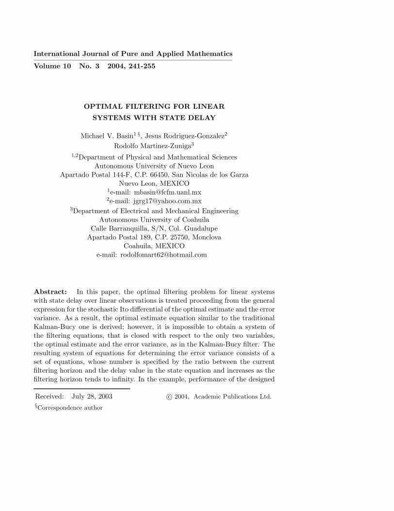
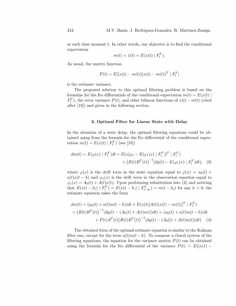
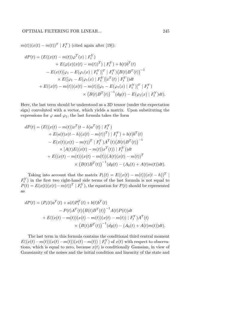
Figure 1: Graphs of the reference state variable x(t) and the estimatesmK(t) and m(t) on the entire simulation interval [0, 10]

unknown matrix P2(t). The equation for the matrix P2(t) is obtained directlyform the equation (6) by changing h to 2h in the definition of P1(t):

dP2(t) = (a(t)P1(t− h) + P3(t)aT (t− 2h))dt

+1

2(b(t)bT (t− 2h) + b(t− 2h)bT (t))dt

− P (t)AT (t)(B(t)BT (t))−1(B(t)BT (t− 2h))

× (B(t− 2h)BT (t− 2h))−1A(t− 2h)P (t− 2h)dt. (7)

The equation (7) for P2(t) depends on the unknown matrix P3(t) = E((x(t)−m(t))(x(t−3h))T | F Y

t ), the equation for P3(t) will depend on P4(t) = E((x(t)−m(t))(x(t − 4h))T | F Y

t ), and so on. Thus, to obtain a closed system of thefiltering equations for the state (1) over the observations (2), the following equa-tions for matrices Pi(t) = E((x(t) −m(t))(x(t − ih))T | F Y

t ), i ≥ 1, should be

248 M.V. Basin, J. Rodriguez-Gonzalez, R. Martinez-Zuniga

7.99 7.992 7.994 7.996 7.998 8 8.002 8.004 8.006 8.008 8.0117.4

17.45

17.5

17.55

time

stat

e

7.99 7.992 7.994 7.996 7.998 8 8.002 8.004 8.006 8.008 8.0117.65

17.7

17.75

17.8

17.85

time

Kal

man

est

imat

e

7.99 7.992 7.994 7.996 7.998 8 8.002 8.004 8.006 8.008 8.0117.4

17.5

17.6

17.7

17.8

time

Opt

imal

est

imat

e

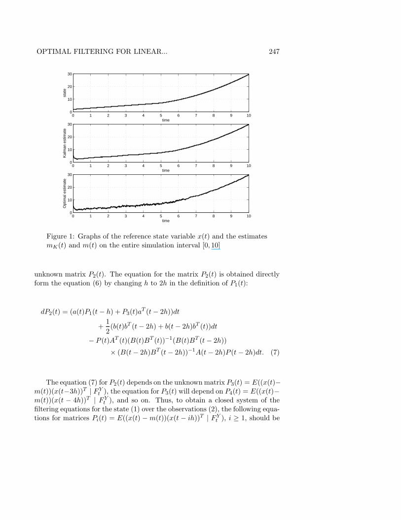
Figure 2: Graphs of the reference state variable x(t) and the estimatesmK(t) and m(t) around the reference time point T = 8

OPTIMAL FILTERING FOR LINEAR... 249

8.99 8.992 8.994 8.996 8.998 9 9.002 9.004 9.006 9.008 9.0122.9

22.95

23

23.05

23.1

time

stat

e

8.99 8.992 8.994 8.996 8.998 9 9.002 9.004 9.006 9.008 9.0123.2

23.25

23.3

23.35

time

Kal

man

est

imat

e

8.99 8.992 8.994 8.996 8.998 9 9.002 9.004 9.006 9.008 9.0123

23.02

23.04

23.06

23.08

time

Opt

imal

est

imat

e

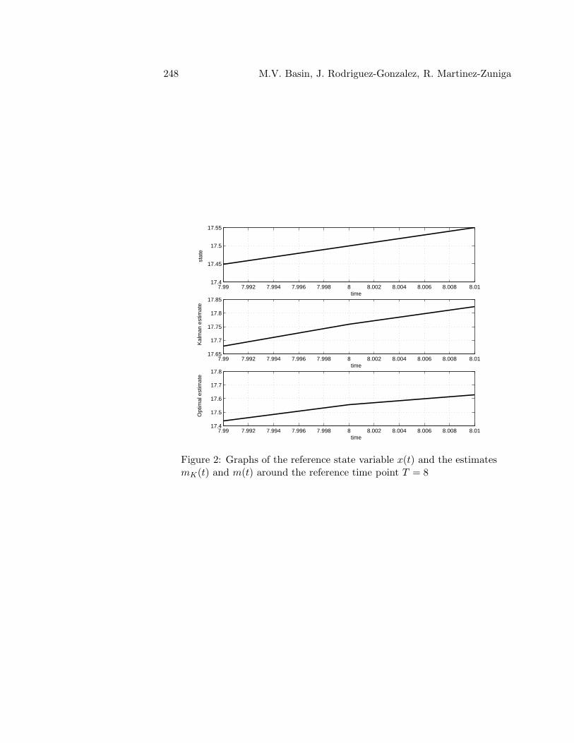
Figure 3: Graphs of the reference state variable x(t) and the estimatesmK(t) and m(t) around the reference time point T = 9

included

dPi(t) = (a(t)Pi−1(t− h) + Pi+1(t)aT (t− ih))dt

+1

2(b(t)bT (t− ih) + b(t− ih)bT (t))dt

− P (t)AT (t)(B(t)BT (t))−1(B(t)BT (t− ih))(B(t − ih)BT (t− ih))−1

×A(t− ih)P (t− ih)dt. (8)

It should be noted that, for every fixed t, the number of equations in (8),that should be taken into account to obtain a closed system of the filteringequations, is not equal to infinity, since the matrices a(t), b(t), A(t), and B(t)are not defined for t < t0. Therefore, if the current time moment t belongs tothe semi-open interval (kh, (k+1)h], where h is the delay value in the equation(1), the number of equations in (8) is equal to k.

The last step is to establish the initial conditions for the system of equations(4), (5), (8). The initial conditions for (4) and (5) are stated as

m(s) = E(φ(s)), s ∈ [t0 − τ, t0) and m(t0) = E(φ(t0) | FYt0

), s = t0, (9)

250 M.V. Basin, J. Rodriguez-Gonzalez, R. Martinez-Zuniga

9.99 9.991 9.992 9.993 9.994 9.995 9.996 9.997 9.998 9.999 1029.42

29.44

29.46

29.48

29.5

time

stat

e

9.99 9.991 9.992 9.993 9.994 9.995 9.996 9.997 9.998 9.999 1029.7

29.72

29.74

29.76

time

Kal

man

est

imat

e

9.99 9.991 9.992 9.993 9.994 9.995 9.996 9.997 9.998 9.999 1029.494

29.496

29.498

29.5

29.502

time

Opt

imal

est

imat

e

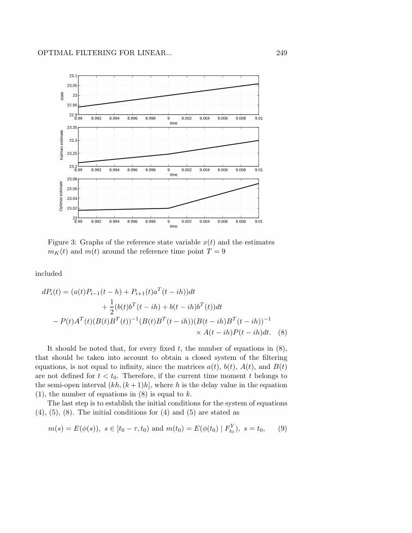
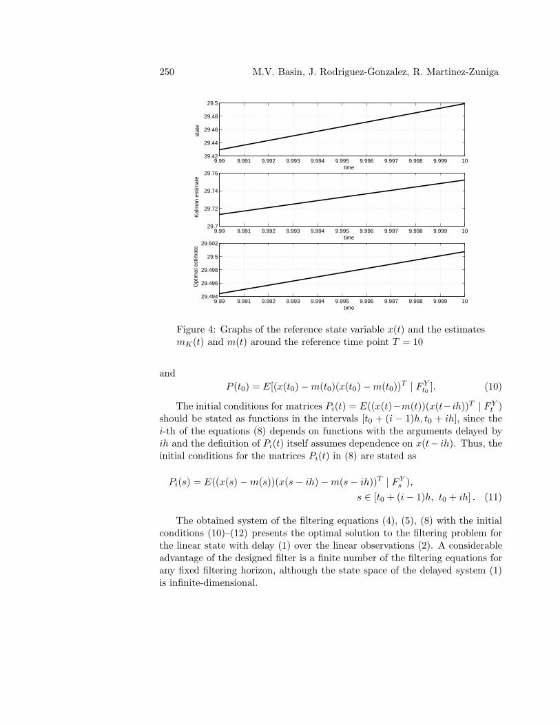
Figure 4: Graphs of the reference state variable x(t) and the estimatesmK(t) and m(t) around the reference time point T = 10

and

P (t0) = E[(x(t0) −m(t0)(x(t0) −m(t0))T | F Y

t0]. (10)

The initial conditions for matrices Pi(t) = E((x(t)−m(t))(x(t−ih))T | F Yt )

should be stated as functions in the intervals [t0 + (i − 1)h, t0 + ih], since thei-th of the equations (8) depends on functions with the arguments delayed byih and the definition of Pi(t) itself assumes dependence on x(t− ih). Thus, theinitial conditions for the matrices Pi(t) in (8) are stated as

Pi(s) = E((x(s) −m(s))(x(s − ih) −m(s− ih))T | F Ys ),

s ∈ [t0 + (i− 1)h, t0 + ih] . (11)

The obtained system of the filtering equations (4), (5), (8) with the initialconditions (10)–(12) presents the optimal solution to the filtering problem forthe linear state with delay (1) over the linear observations (2). A considerableadvantage of the designed filter is a finite number of the filtering equations forany fixed filtering horizon, although the state space of the delayed system (1)is infinite-dimensional.

OPTIMAL FILTERING FOR LINEAR... 251

Remark. The convergence properties of the obtained optimal estimate(4) are given by the standard convergence theorem (see, for example, [11]): ifin the system (1), (2) the pair (a(t), b(t)) is uniformly completely controllableand the pair (a(t), A(t) is uniformly completely observable, then the error ofthe obtained optimal filter (4), (5), (8) is uniformly asymptotically stable. Asusual, the uniform complete controllability condition is required for assuringnon-negativeness of the variance matrix P (t) (5) and may be omitted, if thematrix P (t) is non-negative in view of its intrinsic properties. The uniformcomplete controllability and observability conditions for a linear system withdelay (1) and observations (2) can be found in [18].

4. Example

This section presents an example of designing the optimal filter for a linear statewith delay over linear observations and comparing it to the best filter availablefor a linear state without delay, that is the Kalman-Bucy filter [12].

Let the unobserved state x(t) with delay be given by

x(t) = x(t− 5), x(s) = φ(s), s ∈ [−5, 0], (12)

where φ(s) = N(0, 1) for s ≤ 0, and N(0, 1) is a Gaussian random variable withzero mean and unit variance. The observation process is given by

y(t) = x(t) + ψ(t), (13)

where ψ(t) is a white Gaussian noise, which is the weak mean square derivativeof a standard Wiener process (see [19]). The equations (12) and (13) presentthe conventional form for the equations (1) and (2), which is actually used inpractice [4].

The filtering problem is to find the optimal estimate for the linear state withdelay (12), using direct linear observations (13) confused with independent andidentically distributed disturbances modeled as white Gaussian noises. Let usset the filtering horizon time to T = 10. Since 10 ∈ (1× 5, 2× 5], where 5 is thedelay value in the state equation (12), the only first of the equations (8), alongwith the equations (4) and (5), should be employed.

The filtering equations (4), (5), and the first of the equations (8) take thefollowing particular form for the system (12), (13)

m(t) = m(t− 5) + P (t)[y(t) −m(t)], (14)

252 M.V. Basin, J. Rodriguez-Gonzalez, R. Martinez-Zuniga

with the initial condition m(s) = E(φ(s)) = 0, s ∈ [−5, 0) and m(0) = E(φ(0) |y(0)) = m0, s = 0;

P (t) = 2P1(t) − P 2(t), (15)

with the initial condition P (0) = E((x(0) −m(0))2 | y(0)) = P0; and

P1(t) = 2P (t− 5) + P2(t) − P (t)P (t− 5), (16)

with the initial condition P1(s) = E((x(s) −m(s))(x(s− 5) −m(s− 5)) | F Ys ),

s ∈ [0, 5]; finally, P2(s) = E((x(s) − m(s))(x(s − 10) − m(s − 10)) | F Ys ),

s ∈ [5, 10]. The particular forms of the equations (12) and (14) and the initialcondition for x(t) imply that P1(s) = P0 for s ∈ [0, 5] and P2(s) = P0 fors ∈ [5, 10].

The estimates obtained upon solving the equations (14)–(16) are comparedto the conventional Kalman-Bucy estimates satisfying the following filteringequations for the linear state with delay (12) over linear observations (13),where the variance equation is a Riccati one and the equations for matricesPi(t), i ≥ 1, are not employed:

mK(t) = mK(t− 5) + PK(t)[y(t) −mK(t)], (17)

with the initial condition mK(s) = E(φ(s)) = 0, s ∈ [−5, 0) and mK(0) =E(φ(0) | y(0)) = m0, s = 0;

˙PK(t) = 2PK(t) − P 2K(t), (18)

with the initial condition PK(0) = E((x(0) −m(0))2 | y(0)) = P0.Numerical simulation results are obtained solving the systems of filtering

equations (14)–(16) and (17)–(18). The obtained values of the estimates m(t)and mK(t) satisfying (14) and (17) respectively are compared to the real valuesof the state variable x(t) in (12).

For each of the two filters (14)–(16) and (17)–(18) and the reference system(12) involved in simulation, the following initial values are assigned: x0 = 2,m0 = 10, P0 = 100. Gaussian disturbances ψ1(t) and ψ2(t) in (9) are realizedusing the built-in MatLab white noise function.

The following graphs are obtained: graphs of the reference state variablex(t) for the system (12); graphs of the Kalman-Bucy filter estimate mK(t) satis-fying the equations (17)–(18); graphs of the optimal delayed state filter estimatem(t) satisfying the equations (14)–(16). The graphs of all those variables areshown on the entire simulation interval from T = 0 to T = 10 (Figure 1), andaround the reference time points: T = 8 (Figure 2), T = 9 (Figure 3), and

OPTIMAL FILTERING FOR LINEAR... 253

T = 10 (Figure 4). It can also be noted that the error variance P (t) convergesto zero, since the optimal estimate (14) converges to the real state (12).

The following values of the reference state variable x(t) and the estimatesm(t) and mK(t) are obtained at the reference time points: for T = 8, x(8) =17.5, m(8) = 17.55, mK(8) = 17.76; for T = 9, x(9) = 23.0, m(9) = 23.02,mK(9) = 23.24; for T = 10, x(10) = 29.5, m(10) = 29.5, mK(0) = 29.75.

Thus, it can be concluded that the obtained optimal filter for a linear statewith delay over linear observations (14)–(16) yield definitely better estimatesthan the conventional Kalman-Bucy filter. Subsequent discussion of the ob-tained simulation results can be found in Section 5.

5. Conclusions

The simulation results show that the values of the estimate calculated by usingthe obtained optimal filter for a linear state with delay over linear observationsare noticeably closer to the real values of the reference variable than the val-ues of the Kalman-Bucy estimates. Moreover, it can be seen that the estimateproduced by the optimal filter for a linear state with delay over linear obser-vations asymptotically converges to the real values of the reference variableas time tends to infinity, although the reference system (12) itself is unstable.On the contrary, the conventionally designed (non-optimal) Kalman-Bucy es-timates do not converge to the real values. This significant improvement inthe estimate behavior is obtained due to the more careful selection of the filtergain matrix using the multi-equational system (15)–(16), which compensates forunstable dynamics of the reference system, as it should be in the optimal fil-ter. Although this conclusion follows from the developed theory, the numericalsimulation serves as a convincing illustration.

References

[1] C.T. Abdallah, K. Gu, S. Niculescu, Eds., Proc. 3-rd IFAC Workshop on

Time Delay Systems, Omnipress, Madison (2001).

[2] H.L. Alexander, State estimation for distributed systems with sensing de-lay, SPIE. Data Structures and Target Classification, 1470 (1991).

[3] R.L. Alford, E.B. Lee, Sampled data hereditary systems: linear quadratictheory, IEEE Trans. Automat. Contr., AC–31, (1986), 60-65.

254 M.V. Basin, J. Rodriguez-Gonzalez, R. Martinez-Zuniga

[4] K.J. Astrom, Introduction to Stochastic Control Theory, Academic Press,New York (1970).

[5] E.K. Boukas, Z.K. Liu, Deterministic and Stochastic Time-Delayed Sys-

tems, Birkhauser (2002).

[6] M.C. Delfour, The linear quadratic control problem with delays in spaceand control variables: a state space approach, SIAM. J. Contr. Optim.,24 (1986), 835–883.

[7] J.M. Dion, Linear Time Delay Systems, Pergamon, London (2001).

[8] J.L. Dugard, E.I. Verriest, Eds., Stability and Control of Time-Delay Sys-

tems, Springer (1997).

[9] D.H. Eller, J.K. Aggarwal, H.T. Banks, Optimal control of linear time-delay systems, IEEE Trans. Automat. Contr., AC–14 (1969), 678–687.

[10] F.H. Hsiao, S.T. Pan, Robust Kalman filter synthesis for uncertain mul-tiple time-delay stochastic systems, ASME Transactions., J. of Dynamic

Systems, Measurement, and Control, 118 (1996), 803-807.

[11] A.H. Jazwinski, Stochastic Processes and Filtering Theory, AcademicPress, New York (1970).

[12] R.E. Kalman, R.S. Bucy, New results in linear filtering and predictiontheory, ASME Trans., Part D: J. of Basic Engineering, 83 (1961), 95-108.

[13] E. Kaszkurewicz, A. Bhaya, Discrete-time state estimation with two coun-ters and measurement delay, In: Proc. 35-th IEEE Conf. on Decision and

Control, Kobe, Japan (December 1996).

[14] V.B. Kolmanovskii, A.D. Myshkis, Introduction to the Theory and Appli-

cations of Functional Differential Equations, Kluwer, New York (1999).

[15] V.B. Kolmanovskii, L.E. Shaikhet, Control of Systems with Aftereffect,American Mathematical Society, Providence (1996).

[16] T.D. Larsen, N.A. Andersen, O. Ravn, N. K. Poulsen, Incorporation ofthe time-delayed measurements in a discrete-time Kalman filter, In: Proc.

37-th Conf. on Decision and Control, Tampa, FL (December 1998), 3972–3977.

OPTIMAL FILTERING FOR LINEAR... 255

[17] M.S. Mahmoud, Robust Control and Filtering for Time-Delay Systems,Marcel Dekker, New York (2000).

[18] M. Malek-Zavarei, M. Jamshidi, Time-Delay Systems: Analysis, Optimiza-

tion and Applications, North-Holland, Amsterdam (1987).

[19] V.S. Pugachev, I.N. Sinitsyn, Stochastic Systems: Theory and Applica-

tions, World Scientific (2001).

[20] K. Uchida, E. Shimemura, T. Kubo, N. Abe, The linear-quadratic opti-mal control approach to feedback control design for systems with delay,Automatica, 24 (1988), 773-780.

256