Optimal Experimental Design in the Modelling of Pattern Formation

Optimal Experimental Design in the Modelling

of Pattern Formation

Adrian Lopez Garcıa de Lomana, Alex Gomez-Garrido, David Sportouch, andJordi Villa-Freixa

Grup de Recerca en Informatica Biomedica, IMIM-Universitat Pompeu Fabra,C/Doctor Aiguader, 88, 08003 Barcelona, Catalunya, Spain

{adrianlopezgarciadelomana,david.sportouch}@gmail.com

{agomez,jvilla}@imim.es

http://cbbl.imim.es

Abstract. Gene regulation plays a major role in the control of develop-mental processes. Pattern formation, for example, is thought to be reg-ulated by a limited number genes translated into transcription factorsthat control the differential expression of other genes in different cells ina given tissue. We focused on the Notch pathway during the formation ofchess-like patterns along development. Simplified models exist of the pat-terning by lateral inhibition due to the Notch-Delta signalling cascade.We show here how parameters from the literature are able to explain thesteady-state behavior of model tissues of several sizes, although they arenot able to reproduce time series of experiments. In order to refine theparameters set for data from real experiments we propose a practical im-plementation of an optimal experimental design protocol that combinesparameter estimation tools with sensitivity analysis, in order to minimizethe number of additional experiments to perform.

Key words: lateral inhibition, GRN, optimal experimental design, mul-ticellular system

1 Introduction

One of the most breathtaking processes in biology is the development of a com-plex creature. In a matter of just a day (a fly maggot), a few weeks (a mouse)or several months (ourselves), an egg grows into millions, billions, or, in the caseof humans, 10 trillion cells formed into organs, tissues and parts of the body.So, the main question in developmental biology is to understand how do cellsarising from division of a single cell become different from each other. The com-plexity of the process of pattern formation in developmental biology has beendealt with by a number of researchers in the last decades (for reviews see [1]),both topologically, studying the different genes involved in the process and theirrelationships, and dynamically, measuring and modeling the temporal behav-ior of those genes and their products. Different simulation methods have beenapplied to dynamical models of patterning, involving both ordinary (ODE) [2]

2 Optimal Experimental Design on Pattern Formation Modelling

and partial (PDE) differential equations or discrete representations of the cellsas cellular automata, among others[3]. Initial models for pattern formation werebased on simple assumptions that were able to capture most of the relevant in-formation for a given general question. Thus, it is worth noting the efforts ofMeinhardt [4] and others [5] in order to unravel the general rules governing theformation of complex patterns during the embryo development by using simplealthough soundable mathematical models.

At times, high throughput studies can be also performed in order to obtaintime dependent qualitative information on the topology of the GRN. This typeof information can be processed by probability and statistical inference tools thatcomplement the verbal models defined by the experimentalists and provide a firstformal model of the network. However, if one is able to quantify the dynamicalinformation about the expression levels of different genes, even at the level of afew key genes by, for example, real time polymerase chain reaction (RT-PCR)experiments, global optimization protocols can be used to refine the parametersthat describe the dynamics of the model.

In typical situations the modeller claims for experimental data that is scarce,low quality and, more importantly in most cases, difficult to obtain. How tomaximize the outcome from limited resources is the aim of this paper. Here wepresent the implementation of a practical optimal experimental design pipelinein a theory/experiment integrated fashion. We demonstrate the utility of theprotocol in the parameter estimation for one of the simplest models of pat-tern formation in biology, namely the Notch-Delta pathway for lateral inhibition(LI). To demonstrate the implementation of the method, we work with fictitiousRT-PCR experimental data obtained from known models of the Notch-Delta in-teraction, as the LI model occurs between partner cells in a tissue, which offersan extra challenge for experimental manipulation. However, the proposed pro-tocol is completely general for a RT-PCR experimental setting in any biologicalsystem that suits this technique.

2 Methods

2.1 Problem Statement

As outlined in the introduction, dynamical biological systems can be describedby a large variety of mathematical models. Here we will restrict ourselves tomodels defined in terms of ODEs. Following [6], the time evolution of a systemstate of K species x(t, θ) ∈ R

K is solution of this set of ODEs:

{

∂∂t

x(t, θ) = f(x(t, θ), θ,u(t)).

x(0) = x0.(1)

Here θ∈RP denotes the parameters of the system, and u(t) is a vector containing

the input of the system. The L properties of the system yM (t, θ)∈RLi that can

OED in Pattern Formation Modelling 3

be measured are described by an observation function g at time ti, i = 1, ..., N

(N is here the number of design points):

yM (ti, θ, u) = g(x(ti, θ,u)), i = 1, ..., N. (2)

The observations YD(ti)∈RLi , i = 1, ..., N are considered as random variables

and are given by

YD(ti) = yM (ti, θ0,u) + ǫi, i = 1, ..., N, (3)

where θ0 is the true parameter vector and ǫi∈RLi , i = 1, ..., N describes the

distribution error at time ti. We assume that the distribution of the noise (ob-servation error) follows a normal law (where the variances σ2

ij can be estimatedfrom repetitions of the experiments):

ǫij ∼ N (0, σ2ij), j = 1, ..., Li i = 1, ..., N. (4)

In fact, yM (t, θ) refers to theoretical values (given by the model) and yD(ti)(realizations of the random variables YD(ti)) refers to practical values (it cor-responds to the Li measurements made experimentally at each time ti, i =1, ..., N).

Maximum Likelihood Method This method will help us to get estimates ofthe parameters of the system. In this method, we need to maximize the likelihoodfunction Jml(θ) to get estimates of the parameter vector θ. This function isdefined as:

Jml(θ;yD(t1), . . . ,yD(tN )) = f(YD(t1),...,YD(tN ))(y

D(t1), ...,yD(tN )). (5)

As defined the random variables YD(ti) follow a multivariate normal law

YD(ti) ∼ NL(yM (ti, θ, u), C(ti)), i = 1, ..., N, (6)

where C(ti)∈ML,L(R) is the covariance matrix defined as Cll(ti) = σ2il and

Ckl(ti) = 0 if k 6= l.

Jml(θ;yD(t1), . . . , yD(tN )) =

1

(2π)NL2

v

u

u

u

t

NY

i=1

LiY

j=1

σ2ij

e

−

1

2

NX

i=1

LiX

j=1

yDj (ti) − yM

j (ti, θ, u)

σij

!2

. (7)

Maximizing the likelihood function (regarding of θ) is in fact the same as max-imizing the logarithm of the likelihood function, which in turn is the same asminimizing the opposite of the logarithm of the likelihood function.So, this leadsto minimize the following function:

−ln(Jml(θ; yD(t1), . . . , y

D(tN )) =NL

2+

1

2

NX

i=1

LiX

j=1

ln(σ2ij) +

1

2

NX

i=1

LiX

j=1

yDj (ti) − yM

j (ti, θ, u)

σij

!2

.

(8)

4 Optimal Experimental Design on Pattern Formation Modelling

So, this comes to minimize the following function:

χ2(θ) =

N∑

i=1

Li∑

j=1

(

yDj (ti) − yM

j (ti, θ, u)

σij

)2

. (9)

This corresponds to the minimization of a weighted residual sum of squares(with weights: wij = 1

σ2ij

) to get the estimated parameters.At this point, we can

compute analytically asymptotic estimates of the parameters θ and asymptoticconfidence intervals. In this scope, we assume that we are in the case wherewe have so much observations that the deviation ∆θ between the real θ0 andestimated parameters θ is small. Thus, we can expand the observation functionin a Taylor series:

yMj (ti, θ, u) = yM

j (ti, θ0, u) + ∇θyj |ti,θ0(θ − θ0). (10)

We insert this result in the function to minimize, and we get:

χ2(θ) =

N∑

i=1

Li∑

j=1

[ ǫ2ij

σ2ij

− 2ǫij

σ2ij

∇θyj |ti,θ0∆θ +

1

σ2ij

∆θT ([∇θyj]

T [∇θyj])|ti,θ0∆θ

]

.

(11)To minimize χ2(θ), we need to solve the following equation: ∂

∂θχ2(θ) = 0, so we

get the estimated parameters:

∆θ = F−1N∑

i=1

Li∑

j=1

ǫij

σ2ij

([∇θyj]T )|ti,θ0

. (12)

where F is the Fisher information matrix.

Parameter Estimation and Covariance Matrix From the knowledge of F

we can easily get the exact values of the (asymptotic) estimated parameters:

θ = θ0 + F−1N∑

i=1

Li∑

j=1

ǫij

σ2ij

([∇θyj ]T )|ti,θ0

. (13)

As we assumed that the residuals are independently distributed, the covariancematrix of the estimated parameter vector is computed by (where the average isover the repetition of experiments):

Σ =< ∆θ∆θT >= F−1. (14)

Thanks to this covariance matrix, we can see the correlation between the pa-rameters. The correlation matrix is defined by:

{

Rij =Σij√ΣiiΣjj

, if i 6= j.

Rij = 1, if i = j.(15)

OED in Pattern Formation Modelling 5

2.2 Parameter Correlation and Identifiability Criteria

Equipped with Eqn. (15), we can measure the interrelationship between the pa-rameters and get an idea of the compensation effects of changes in the parametervalues on the model output. For instance, if two parameters are highly correlated,a change in the model output caused by a change in a model parameter can becompensated by an appropriate change in the other parameter value. This pre-vents such parameters from being uniquely identifiable even if the model outputis very sensitive to changes to individual parameters.

Then we can try to improve the information contained in the data by op-timizing one of the criteria derived from Σ. We used the modified E-optimal

design: min(λmax(Σ)λmin(Σ) ). As it minimizes the ratio of the largest to the smallest

eigenvalue, it optimizes the functional shape of the confidence intervals. All cal-culations have been performed with ByoDyn (http://cbbl.imim.es/ByoDyn)most of them at the QosCosGrid [7] environment.

3 Results

3.1 The ODEs Model for the Notch-Delta System

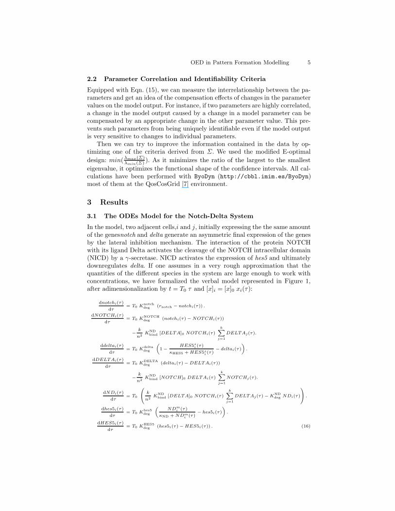
In the model, two adjacent cells,i and j, initially expressing the the same amountof the genesnotch and delta generate an asymmetric final expression of the genesby the lateral inhibition mechanism. The interaction of the protein NOTCHwith its ligand Delta activates the cleavage of the NOTCH intracellular domain(NICD) by a γ-secretase. NICD activates the expression of hes5 and ultimatelydownregulates delta. If one assumes in a very rough approximation that thequantities of the different species in the system are large enough to work withconcentrations, we have formalized the verbal model represented in Figure 1,after adimensionalization by t = T0 τ and [x]i = [x]0 xi(τ):

dnotchi(τ)

dτ= T0 K

notchdeg (rnotch − notchi(τ)) .

dNOTCHi(τ)

dτ= T0 K

NOTCHdeg (notchi(τ) − NOTCHi(τ))

−

k

n2K

NDbind [DELTA]0 NOTCHi(τ)

kX

j=1

DELTAj(τ).

ddeltai(τ)

dτ= T0 K

deltadeg

„

1 −

HES5si (τ)

κHES5 + HES5si(τ)

− deltai(τ)

«

.

dDELTAi(τ)

dτ= T0 K

DELTAdeg (deltai(τ) − DELTAi(τ))

−

k

n2K

NDbind [NOTCH]0 DELTAi(τ)

kX

j=1

NOTCHj(τ).

dNDi(τ)

dτ= T0

0

@

k

n2K

NDbind [DELTA]0 NOTCHi(τ)

kX

j=1

DELTAj(τ) − KNDdeg NDi(τ)

1

A .

dhes5i(τ)

dτ= T0 K

hes5deg

„

NDmi (τ)

κND + NDmi

(τ)− hes5i(τ)

«

.

dHES5i(τ)

dτ= T0 K

HES5deg (hes5i(τ) − HES5i(τ)) . (16)

6 Optimal Experimental Design on Pattern Formation Modelling

where we have assumed that the NOTCH cleavage after the formation of the NDcomplex, the NICD transport to the nucleus and the transcription factor activa-tion can be simply approximated by the amount of ND complex that is formedon the membrane surface. In 16 notch is constitutively activated, while sigmoidalactivation and inhibition curves are used for hes5 and delta, respectively.

Fig. 1. Simplified model for the Notch/Delta pathway for two adjacent cells i

and j. NOTCH* and DELTA* refers to the activated forms.

By using the parameters Khes5deg = KHES5

deg = KNOTCHdeg = KDELTA

deg = KNDdeg =

Kdeltadeg = 0.01; s = m = 2.0; κND = κHES5 = 0.1; NOTCH0 = 5.0; Knotch

deg =

0.0016649; KNDbind = 0.25; DELTA0 = 3.0; rnotch = 0.620926, the steady state

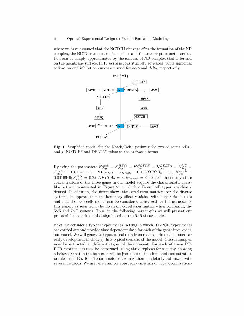
concentrations of the three genes in our model acquire the characteristic chess-like pattern represented in Figure 2, in which different cell types are clearlydefined. In addition, the figure shows the correlation matrices for the diversesystems. It appears that the boundary effect vanishes with bigger tissue sizesand that the 5×5 cells model can be considered converged for the purposes ofthis paper, as seen from the invariant correlation matrix when comparing the5×5 and 7×7 systems. Thus, in the following paragraphs we will present ourprotocol for experimental design based on the 5×5 tissue model.

Next, we consider a typical experimental setting in which RT-PCR experimentsare carried out and provide time dependent data for each of the genes involved inour model. We will generate hypothetical data from real experiments of inner earearly development in chick[8]. In a typical scenario of the model, 4 tissue samplesmay be extracted at different stages of development. For each of them RT-PCR experiments may be performed, using three replicas for security, showinga behavior that in the best case will be just close to the simulated concentrationprofiles from Eq. 16. The parameter set θ may then be globally optimized withseveral methods. We use here a simple approach consisting on local optimizations

OED in Pattern Formation Modelling 7

a.

delta delta delta delta

b.

DELTA_0

K_bind_ND

K_deg_DELTA

K_deg_HES5

K_deg_ND

K_deg_NOTCH

K_deg_delta

K_deg_hes5

K_deg_notch

NOTCH_0

kappa_HES5

kappa_ND

m r_notch

s

DELTA_0

K_bind_ND

K_deg_DELTA

K_deg_HES5

K_deg_ND

K_deg_NOTCH

K_deg_delta

K_deg_hes5

K_deg_notch

NOTCH_0

kappa_HES5

kappa_ND

m

r_notch

s

DELTA_0

K_bind_ND

K_deg_DELTA

K_deg_HES5

K_deg_ND

K_deg_NOTCH

K_deg_delta

K_deg_hes5

K_deg_notch

NOTCH_0

kappa_HES5

kappa_ND

m r_notch

s

DELTA_0

K_bind_ND

K_deg_DELTA

K_deg_HES5

K_deg_ND

K_deg_NOTCH

K_deg_delta

K_deg_hes5

K_deg_notch

NOTCH_0

kappa_HES5

kappa_ND

m

r_notch

s

DELTA_0

K_bind_ND

K_deg_DELTA

K_deg_HES5

K_deg_ND

K_deg_NOTCH

K_deg_delta

K_deg_hes5

K_deg_notch

NOTCH_0

kappa_HES5

kappa_ND

m r_notch

s

DELTA_0

K_bind_ND

K_deg_DELTA

K_deg_HES5

K_deg_ND

K_deg_NOTCH

K_deg_delta

K_deg_hes5

K_deg_notch

NOTCH_0

kappa_HES5

kappa_ND

m

r_notch

s

DELTA_0

K_bind_ND

K_deg_DELTA

K_deg_HES5

K_deg_ND

K_deg_NOTCH

K_deg_delta

K_deg_hes5

K_deg_notch

NOTCH_0

kappa_HES5

kappa_ND

m r_notch

s

DELTA_0

K_bind_ND

K_deg_DELTA

K_deg_HES5

K_deg_ND

K_deg_NOTCH

K_deg_delta

K_deg_hes5

K_deg_notch

NOTCH_0

kappa_HES5

kappa_ND

m

r_notch

s

Fig. 2. (a.) Delta steady state concentration distribution in model tissues ofdifferent dimensions. (b.) Correlation matrices of the adimensional parametersin each case in (a). The steady state is achieved at a biologically plausible timescale.

from 10 or 100 starting random values of θ with varying value of σ2 for thegenerated data points.

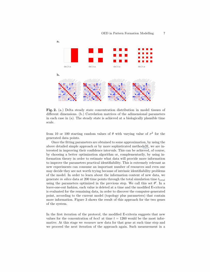
Once the fitting parameters are obtained to some approximation, by using theabove detailed simple approach or by more sophisticated methods[9], we are in-terested in improving their confidence intervals. This can be achieved, of course,by choosing a better optimization algorithm or, complementarily, by using in-formation theory in order to estimate what data will provide more informationto improve the parameters practical identifiability. This is extremely relevant asnew experiments can consume an important number of resources and even onemay decide they are not worth trying because of intrinsic identifiability problemsof the model. In order to learn about the information content of new data, wegenerate in silico data at 200 time points through the total simulation time ttotalusing the parameters optimized in the previous step. We call this set θ′. In aleave-one-out fashion, each value is deleted at a time and the modified E-criteriais evaluated for the remaining data, in order to discover the computer-generatedpoint, according to the current model (topology plus parameters) that containmore information. Figure 3 shows the result of this approach for the two genesof the system.

In the first iteration of the protocol, the modified E-criteria suggests that newvalues for the concentration of hes5 at time t = 1260 would be the most infor-mative. At this stage we measure new data for that gene at such time step andwe proceed the next iteration of the approach again. Such measurement in a

8 Optimal Experimental Design on Pattern Formation Modelling

0 200 400 600 800 1000 1200 1400Time

1000000

1500000

2000000

2500000

3000000

3500000

4000000

4500000

ME c

rite

ria

model

deltahes5

Fig. 3. Modified E-criteria after adding one time point per gene at each timefrom a set of previous targeted behavior.

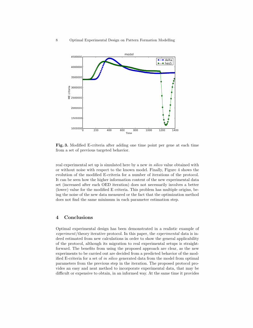
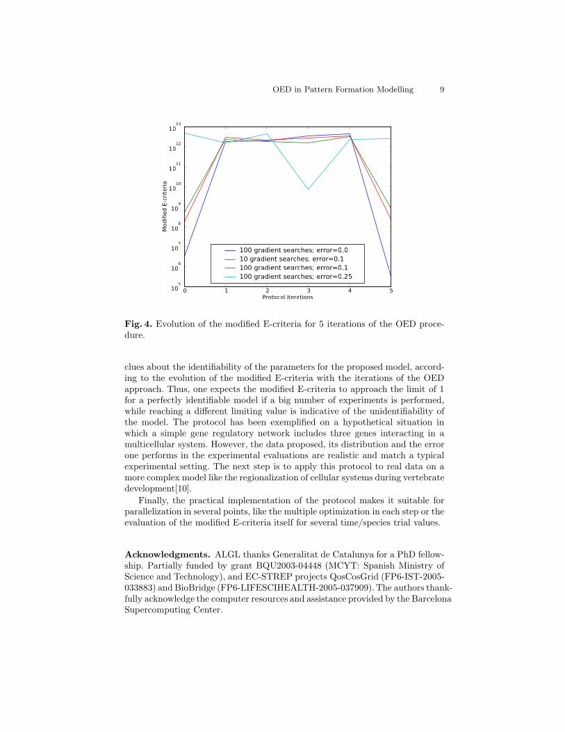
real experimental set up is simulated here by a new in silico value obtained withor without noise with respect to the known model. Finally, Figure 4 shows theevolution of the modified E-criteria for a number of iterations of the protocol.It can be seen how the higher information content of the new experimental dataset (increased after each OED iteration) does not necessarily involves a better(lower) value for the modified E criteria. This problem has multiple origins, be-ing the noise of the new data measured or the fact that the optimization methoddoes not find the same minimum in each parameter estimation step.

4 Conclusions

Optimal experimental design has been demonstrated in a realistic example ofexperiment/theory iterative protocol. In this paper, the experimental data is in-deed estimated from new calculations in order to show the general applicabilityof the protocol, although its migration to real experimental setups is straight-forward. The benefits from using the proposed approach are clear, as the newexperiments to be carried out are decided from a predicted behavior of the mod-ified E-criteria for a set of in silico generated data from the model from optimalparameters from the previous step in the iteration. The proposed protocol pro-vides an easy and neat method to incorporate experimental data, that may bedifficult or expensive to obtain, in an informed way. At the same time it provides

OED in Pattern Formation Modelling 9

0 1 2 3 4 5Protocol iterations

105

106

107

108

109

1010

1011

1012

1013

Modifie

d E

-cri

teri

a

100 gradient searches; error=0.010 gradient searches; error=0.1100 gradient searches; error=0.1100 gradient searches; error=0.25

Fig. 4. Evolution of the modified E-criteria for 5 iterations of the OED proce-dure.

clues about the identifiability of the parameters for the proposed model, accord-ing to the evolution of the modified E-criteria with the iterations of the OEDapproach. Thus, one expects the modified E-criteria to approach the limit of 1for a perfectly identifiable model if a big number of experiments is performed,while reaching a different limiting value is indicative of the unidentifiability ofthe model. The protocol has been exemplified on a hypothetical situation inwhich a simple gene regulatory network includes three genes interacting in amulticellular system. However, the data proposed, its distribution and the errorone performs in the experimental evaluations are realistic and match a typicalexperimental setting. The next step is to apply this protocol to real data on amore complex model like the regionalization of cellular systems during vertebratedevelopment[10].

Finally, the practical implementation of the protocol makes it suitable forparallelization in several points, like the multiple optimization in each step or theevaluation of the modified E-criteria itself for several time/species trial values.

Acknowledgments. ALGL thanks Generalitat de Catalunya for a PhD fellow-ship. Partially funded by grant BQU2003-04448 (MCYT: Spanish Ministry ofScience and Technology), and EC-STREP projects QosCosGrid (FP6-IST-2005-033883) and BioBridge (FP6-LIFESCIHEALTH-2005-037909).The authors thank-fully acknowledge the computer resources and assistance provided by the BarcelonaSupercomputing Center.

10 Optimal Experimental Design on Pattern Formation Modelling

References

1. Tomline, C.J., Axelrod, J.D.: Biology by numbers: mathematical modelling indevelopmental biology. Nature Reviews 8 (2007) 331–340

2. Jaeger, J., Surkova, S., Blagov, M., Janssens, H., Kosman, D., Kozlov, K.N., Manu,Myasnikova, E., Vanario-Alonso, C., Samsonova, M., Sharp, D.H., Reinitz, J.: Dy-namic control of positional information in the early Drosophila embryo. Nature430 (2004) 368–371

3. de Jong, H.: Modeling and simulation of genetic regulatory systems: a literaturereview. J Comput Biol 9(1) (2002) 67–103

4. Meinhardt, H.: Computational modelling of epithelial patterning. Curr Opin GenetDev 17(4) (2007) 272–280

5. von Dassow, G., Meir, E., Munro, E.M., Odell, G.M.: The segment polarity networkis a robust developmental module. Nature 406 (2000) 188–192

6. Faller D, Klingmller U, T.J.: Simulation methods for optimal experimental designin systems biology. Simulation 79 (2003) 717–725

7. Coti, C., Herault, T., Peyronnet, S., Rezmerita, A., Cappello, F.: Grid services forMPI. In ACM/IEEE, ed.: Proceedings of the 8th IEEE International Symposiumon Cluster Computing and the Grid (CCGrid’08), Lyon, France (May 2008)

8. Alsina B., Abello G., U.E.H.D.P.C., F., G.: FGF signaling is required for determi-nation of otic neuroblasts in the chick embryo. Dev. Biol. 267(1) (2004) 119–134

9. Rodriguez-Fernandez, M., Egea, J.A., Banga, J.R.: Novel metaheuristic for pa-rameter estimation in nonlinear dynamic biological systems. BMC Bioinformatics7 (2006) 483

10. Alsina, B., Garcia de Lomana, A., Villa-Freixa, F., Giraldez, F. submitted (2008)