Optimal exit time from casino gambling: strategies of pre-committed …xz2574/download/casino2.pdf · o ered a fair bet, e.g., roulette wheel, in a casino: win or lose one dollar

Optimal exit time from casino gambling: strategies of

pre-committed and naive gamblers

Xue Dong He∗ Sang Hu† Jan Ob loj‡ Xun Yu Zhou§

December 22, 2015

Abstract

We employ the casino gambling model in He et al. (2015) to study the strategies of a pre-

committed gambler, who commits her future selves to the strategy she sets up today, and of

a naive gambler, who fails to do so and thus keeps changing plans at every time. We identify

conditions under which the pre-committed gambler, asymptotically, adopts a stop-loss strategy,

exhibits the behavior of disposition effect, or does not exit. For a specific parameter setting

when the utility function is piece-wise power and the probability weighting functions are concave

power, we derive the optimal strategy of the pre-committed gambler in closed-form whenever

it exists. Finally, we study the actual behavior of the naive gambler and highlight its marked

differences from that of the pre-committed gambler.

Key words: casino gambling, cumulative prospect theory, optimal stopping, pre-committed

gamblers, naive gamblers, optimal strategies

∗Department of Industrial Engineering and Operations Research, Columbia University, Room 315, Mudd Building,500 W. 120th Street, New York, NY 10027, US. Email: [email protected]. The research of this author wassupported by a start-up fund at Columbia University.†Risk Management Institute, National University of Singapore, 21 Heng Mui Keng Terrace, Singapore 119613.

Email: [email protected].‡Mathematical Institute, The Oxford-Man Institute of Quantitative Finance and St John’s College, University

of Oxford, Oxford, UK. Email: [email protected]. Part of this research was completed while this authorwas visiting CUHK in March 2013 and he is grateful for the support from the host. He also gratefully acknowledgessupport from ERC Starting Grant RobustFinMath 335421.§Mathematical Institute, The University of Oxford, Woodstock Road, OX2 6GG Oxford, UK, and Oxford–Man

Institute of Quantitative Finance, The University of Oxford. Email: [email protected]. The research of thisauthor was supported by a start-up fund of the University of Oxford, and research grants from the Oxford–ManInstitute of Quantitative Finance and Oxford–Nie Financial Big Data Lab.

1

1 Introduction

We analyse theoretically, and compare, the behavior of different types of gamblers in a casino

gambling model formulated in our recent paper He et al. (2015). This model was in turn a gen-

eralization of the one initially proposed by Barberis (2012). At time 0, a gambler is offered a fair

bet in a casino: win or lose $1 with equal probability. If the gambler takes the bet, the bet is

played out and she either gains $1 or loses $1 at time 1. Then the gambler is offered the same bet

and she decides whether to play. The same bet is offered and played out repeatedly until the first

time the gambler declines the bet. At that time, the gambler exits the casino with all her prior

gains and losses. The gambler needs to determine the best time to stop playing, with the objective

to maximize her preference value of the final wealth, while the preferences are represented by the

cumulative prospect theory (CPT, Tversky and Kahneman, 1992).

As shown in Barberis (2012), when the gambler uses the same CPT preferences to revisit the

gambling problem in the future, e.g., at time t > 0, the optimal gambling strategy solved at time

0 is typically no longer optimal. This time-inconsistency arises from the probability weighting

in CPT. If the gambler is pre-committed, she commits her future selves to the strategy solved at

time 0. If she fails to pre-commit, namely she keeps changing her strategy in the future, then the

gambler is said to be naive. The actual strategy implemented by a naive gambler will often be very

different from the strategy viewed as optimal at time 0 and which is actually implemented by a

pre-committed gambler.

In our recent paper, He et al. (2015), we illustrate how and why the CPT objectives can be

strictly improved in general by considering path-dependent strategies or by tossing independent

coins1 along the way. Moreover, we show that any path-dependent strategy is equivalent to a

randomization of path-independent strategies. These results justify the enlargement of the set of

feasible strategies to include the randomized ones. Then, in the setting of an infinite time horizon,

we develop a systematic and analytical approach to finding a pre-committed gambler’s optimal

(randomized) strategy; this includes change of decision variable from the stopping time to the

1The observation that using randomized strategies may be strictly beneficial for the gambler was made indepen-dently in Henderson et al. (2015).

2

stopped distribution, formulation of an infinite dimensional program for the latter, and application

of the Skorokhod embedding theory to retrieve the optimal stopping from the optimal stopped

distribution. In summary, He et al. (2015) establishes a theoretical foundation for solving the

casino model, although some of the technical components were left for further research. Most are

tackled in this paper and its online appendix2.

In this paper, we continue to study the optimal strategies of a pre-committed gambler, as well

as the actual strategies implemented by a naive gambler, for the case of an infinite time horizon.

Barberis (2012) considered a five-period model and found these strategies by exhaustive search.

Such an approach quickly becomes very involved and is clearly impossible to use when there is no

end date. Instead, in this paper we are able to derive these strategies analytically which allows us

to build a general theoretical comparison. As far as we know, our paper is the first to analytically

study the strategies of a pre-committed gambler and compare them with those of a naive gambler in

a general discrete time casino gambling setting and using CPT preferences. A similar approach was

recently adopted by Henderson et al. (2015) in a continuous time setting and used to complement

and counter earlier findings in Ebert and Strack (2012). Both of these papers, see Section 5

for discussion, rely on the crucial feature of their setting which allows the gambler to construct

arbitrarily small random payoffs. This feature stands in a clear distinction with our setting and

their results are not applicable here.

We first investigate when the optimal strategy of the pre-committed gambler does not exist

and find asymptotical optimal strategies in this case. We further divide these asymptotical optimal

strategies into three types: loss-exit, gain-exit, and non-exit strategies. In the original terms of

Barberis (2012) (for a five-period model), a loss-exit strategy is to exit at a fixed loss level and not

to exit at any gain level, a gain-exit strategy is the opposite, and a non-exit strategy is not to stop

at any gain and loss levels.3 In the present paper, as the time horizon is infinite and the optimal

CPT value may not be attained, a loss-exit strategy is interpreted as exiting at a certain fixed loss

level or at an asymptotically large gain level (so essentially it only stops at a loss; hence the name).

2Available at http://ssrn.com/abstract=2682637 .3 These three types of strategies mirror respectively the stop-loss, disposition effect (Shefrin and Statman, 1985),

and buy-and-hold strategies or phenomenon in stock trading.

3

Similar interpretations are applied to gain-exit and non-exit strategies. We find conditions under

which the pre-committed gambler takes loss-exit, gain-exit, and non-exit strategies, respectively,

and our theoretical results are consistent with the numerical results in Barberis (2012).

We then assume a piece-wise power utility function and concave, power probability weighting

functions. The concave, power weighting functions, although not typically used in CPT, are still

able to model the overweighing of very small probabilities of large gains and losses. With this

specification of the utility and weighting functions, we are able to derive the optimal strategy of

the pre-committed gambler completely and analytically.

Finally, we study the actual behavior of a naive gambler and compare it with that of the pre-

committed gambler. We find the conditions under which the naive gambler stays at the casino

forever. In particular, we prove that under some conditions, while the pre-committed gambler will

stop for sure before the loss hits a certain level, the naive gambler continues to play with a positive

probability at any loss level.

The remainder of this paper is organized as follows: In Section 2, we recall the casino gambling

model formulated in He et al. (2015). In Section 3, we study the existence of the optimal strategies

and discuss loss-exit, gain-exit, and non-exit strategies. In Section 4, we solve the gambling problem

completely when the utility function is piece-wise power and the probability weighting functions

are power. We then discuss the strategies taken by a naive gambler in Section 5. Finally, Section

6 concludes. Some of the proofs are placed in Appendices at the end of the paper and the others

are placed in an online appendix available at http://ssrn.com/abstract=2682637.

2 The Model

We consider the casino gambling problem formulated in He et al. (2015). At time 0, a gambler is

offered a fair bet, e.g., roulette wheel, in a casino: win or lose one dollar with equal probability. If

the gambler takes the bet, the bet outcome is played out at time 1. Then the gambler is offered

the same bet and she decides whether to play. The same bet is offered and played out repeatedly

until the first time the gambler declines the bet. At that time, the gambler leaves the casino with

all her prior gains and losses. The gambler needs to decide the time τ to exit the casino.

4

Denote by St, t = 0, 1, . . . the cumulative gain or loss of the gambler in the casino at t. Then,

{St : t ≥ 0} is a symmetric random walk. The gambler chooses the exit time τ to maximize her

preference for Sτ , while the preferences are modeled by CPT, assuming the reference point to be

her initial wealth at the time she enters the casino. Then, the gambler’s preference value of Sτ is

V (Sτ ) =

∞∑n=1

u+(n)(w+(P(Sτ ≥ n))− w+(P(Sτ > n))

)−∞∑n=1

u−(n)(w−(P(Sτ ≤ −n))− w−(P(Sτ < −n))

),

(1)

where u+(·) and u−(·) are the utility function of gains and disutility function of losses, respectively,

and w+(·) and w−(·) are the probability weighting functions regarding gains and losses, respectively.

Assume that u±(·) are continuous, increasing, and concave, and satisfy u±(0) = 0. In addition,

w±(·) are increasing mappings from [0, 1] onto [0, 1]. We adopt the convention that ∞−∞ = −∞

so that V (Sτ ) := −∞ if the second sum of infinite series in (1) is +∞.

Let T be the set of stopping times that can be chosen by the gambler at time 0. Then, the

gambler faces the following optimization problem at time 0:

maxτ∈T

V (Sτ ). (2)

Following He et al. (2015), we allow the gambler to use the following randomized strategies: at

each time t, the gambler can toss an independent and (possibly biased) coin to decide whether to

stay in the casino: stay if the outcome is heads and leave otherwise. The probability that the coin

turns up tails may depend on time t and on the cumulative gain/loss St at that time, and this

probability is decided by the gambler as part of the strategy. More precisely, the gambler can take

any strategy in the following set

AC := {τ |τ := inf{t ≥ 0|ξt,St = 0} for some {ξt,x}t≥0,x∈Z that are independent 0-1

random variables and are independent of {St}t≥0.}.

We comment below why there is essentially no loss of generality in considering only such stopping

5

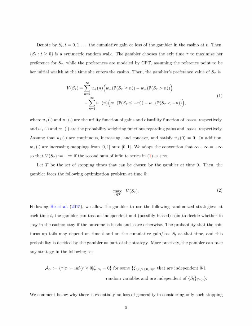
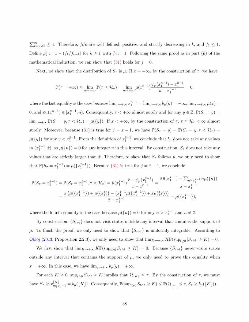
(0,0)

(1,1)

(2,2)

(1,-1)

(2,-2)

(2,0)

Figure 1: Gain/loss process represented as a binomial tree. Each node is marked on its right by a pair(t, x), where t stands for the time and x the amount of (cumulative) gain/loss at that time. For example,the node (2,−2) signifies a total loss, relative to the initial wealth, of $2 at time 2.

times. Finally, we require {Sτ∧t}, t = 0, 1, . . . to be uniformly integrable so as to, among other

things, exclude doubling strategies; so T = {τ ∈ AC |{Sτ∧t} is uniformly integrable}.

In the binomial tree representation of {St}, each node of the tree stands for the current level

of cumulative gain/loss (t, St) and the path leading to this node stands for the historical levels

of cumulative gain/loss; see Figure 1. For instance, following the path starting from node (0,0),

through node (1,1), and leading to node (2,0), the gambler wins $1 in the first bet, loses $1 in the

second bet, and thus ends up with $0 cumulative gain/loss at time 2. At each node, the gambler

can toss a biased coin to decide whether to stay in the casino. Therefore, the gambler’s decision

depends not only on the current level of cumulative gain/loss but also on the outcome of a random

coin that is independent of the bet outcomes in the casino.

In our previous paper, He et al. (2015), we offer explanation why randomized strategies are

in general preferred for a CPT gambler. Moreover, it is shown that, although path-dependent

stopping times, both randomized and non-randomized, are not directly included in AC , they are

equivalent to certain stopping times in AC in terms of the distribution St at the stopping times

and thus lead to the same CPT preference value. One of the main contributions of He et al. (2015)

6

is to establish that the set of the distributions of Sτ for τ ∈ T is

M0(Z) =

{probability measure µ on Z |

∑n∈Z|n| · µ({n}) <∞,

∑n∈Z

n · µ({n}) = 0

}. (3)

Therefore, once the optimal stopped distribution is found in M0(Z), the corresponding optimal

stopping time can be recovered via the Skorokhod embedding. This result is the theoretical foun-

dation for solving (2); see the discussion in He et al. (2015) and the solution in Section 4 of the

present paper.

Here, we make two comments on the set T of feasible exit times. First, any exit strategies

without randomization and satisfying the uniform integrability condition belong to T . In particular,

strategies such as stopping when St hits one of a lower barrier a and an upper barrier b are feasible.

Secondly, randomized strategies in AC are path-independent: the random coin tossed at each time

t, and thus the decision of whether to stay, depends only on the level of cumulative gain/loss at

that time. Note, however, that in general the gambler needs to toss a random coin at every time in

order to implement a strategy in AC . An alternative stopping strategy to realize a same optimal

distribution of St is provided in Appendix B: the gambler only needs to toss a coin occasionally,

but she needs to keep track of the historical maximum of the cumulative gain and loss (hence

path-dependent). This alternative strategy resembles the so-called “trailing stop-loss” strategy in

stock trading. See the discussions in Example 2 and Appendix B.

As shown in Barberis (2012), when the gambler uses the same CPT preferences to revisit the

gambling problem in the future, e.g., at time t > 0, the optimal strategy of problem (2), which is

solved at time 0, is no longer optimal. This arises from the probability weighting function. If the

gambler commits her future selves to the strategy solved at time 0, the optimal strategy of problem

(2) is the one that is implemented by the gambler. In this case, the gambler is sophisticated and

pre-committed. If at each time the gambler fails to commit her future selves to the strategy solved

at that time, she keeps changing her strategy in the future. In this case, the gambler is naive, and

the actual strategy implemented by the gambler is different from the optimal strategy of problem

(2). In the following, we first study the pre-committing strategy, i.e., the optimal strategy of the

pre-committed gambler, in Sections 3 and 4. Then, we study the actual behavior of a naive gambler

7

in Section 5.

The third type of gamblers discussed by Barberis (2012) is called sophisticated gamblers without

pre-commitment, who know their future selves will not follow today’s strategy and thus adjust

today’s strategy accordingly. In the five-period model considered by Barberis (2012), the “optimal”

strategy of such a gambler is defined through a backward induction: starting from the end of the

time horizon when the only choice of the gambler is to leave the casino, at the beginning of each

period, the gambler decides her strategy knowing what her action will be in the following periods.4

In our model, such a definition is impossible because the end of the infinite time horizon does not

exist. Therefore, we opt not to discuss this type of gamblers in our model.

The following usual notations will be used throughout the paper: for any real number x, bxc

stands for the floor of x, i.e., the largest integer dominated by x, and dxe stands for the ceil of x,

i.e., the smallest integer dominating x. For real numbers x and y, x ∧ y := min(x, y).

3 Stop Loss, Disposition Effect, and Non-Exit

In this section, we study various behaviors of pre-committed gamblers via a class of simple two-level

strategies. For two integers b < 0 < a we denote the first exit time from [b, a] by

τa,b := inf{t ≥ 0 : St = a or St = b}.

Theorem 1 Let V ∗ be the value of the optimization problem in (2).

(i) Suppose there exists s > 0 such that

lim infx→+∞

u+(sx)w+(1/x) = +∞. (4)

Then, V ∗ =∞ and there exists b < 0 such that lima→+∞ V (Sτa,b) = +∞.

4It is also called an equilibrium strategy in economics literature.

8

(ii) Suppose there exists ε > 0 such that

lim supx→+∞

u−(x1+ε)w−(1/x) = 0. (5)

Then, V ∗ = supx≥0 u+(x). Moreover, the optimal solution to problem (2) does not exist and

V (Sτa,b) with a = bkε/(1+ε)c and b = −k converges to V ∗ as k goes to infinity.

(iii) Suppose limx→+∞ u+(x) = +∞, and there exists p ∈ (0, 1) such that

lim supx→+∞

u−

(p

1−px)

u+(x)<

w+(p)

w−(1− p). (6)

Then, V ∗ =∞ and there exists c > 0 such that limk→+∞ V (Sτa,b) = +∞ where a = dcke and

b = −k.

Theorem 1 provides three cases in which the optimal solution to problem (2) does not exist.

In the first case, (i), the optimal value of the gambling problem (2) is infinite. The strategy τa,b

the gambler takes, as a→ +∞, is of the “stop-loss-and-let-profit-run” type: to exit once reaching

a fixed loss level −b and not to stop in gain. It is essentially a loss-exit strategy, in Barberis’

term (Barberis, 2012). Such a strategy caps the loss and allows infinite gain, producing a highly

skewed distribution which is favored due to probability weighting. Indeed, consider the following

lottery: winning sx dollars with probability 1/x and winning nothing otherwise, where x is a

sufficiently large number. The expected payoff of the lottery is s and the CPT value of the lottery

is u+(sx)w+(1/x). Therefore, condition (4) implies that the gambler has strong preferences for this

type of highly skewed lotteries so that with limited wealth s, she can achieve infinite CPT value by

purchasing these lotteries.

In case (ii), the optimal value is finite or infinite depending on the whether or not u+ is uniformly

bounded; however either way this value is not attained by any stopping strategy. The gambler likes

the following strategy: leave the casino when losing more than k dollars or when winning more

than bkε/(1+ε)c dollars for sufficiently large k. Note that bkε/(1+ε)c is much smaller than k when

ε is small. For instance, when ε = 0.25 and k = 100000, the strategy taken by the gambler is

9

to stop gambling when winning $10 or when losing $100000. This type of strategy exhibits the

so-called disposition effect, namely, to sell the winners too soon and hold the losers too long (Shefrin

and Statman, 1985). To understand the preferences underlying this sort of behaviors, consider the

following random loss: losing x1+ε dollars with 1/x probability and losing nothing otherwise, where

x is sufficiently large. The expected loss is as large as xε. However, condition (5) implies that the

CPT value of this random loss, −u−(x1+ε)w−(1/x), is nearly zero. Hence, the dispositional effect

is a result of the gambler not willing to pay anything to hedge against the loss, even though the

expected loss is large. It corresponds to an essentially gain-exit strategy.

In case (iii) of Theorem 1, condition (6) is related to the large loss aversion degree (LLAD),

defined as limx→+∞ u−(x)/u+(x), in He and Zhou (2011). Indeed, by setting p = 1/2, condition (6)

is implied by the one that LLAD is strictly less than w+(1/2)/w−(1/2), i.e., LLAD is sufficiently

low. In this case, condition (6) implies that probability weighting on large gains dominates a

combination of weighting on large losses and loss aversion. The corresponding strategy taken by

the gambler is to exit when either the gain reaches a sufficiently high level (bckc) or the loss reaches

another sufficiently high level (k), and these two levels are of the same magnitude. Therefore, we

can consider it to be an essentially non-exit strategy.

We can make the above discussions precise mathematically. For any stopping time τ ∈ T , define

R(τ) :=E[Sτ |Sτ ≥ 1]

E[−Sτ |Sτ ≤ −1]

as the conditional gain-loss ratio. For stopping time τa,b, we have R(τa,b) = a/(−b). Thus, Theorem

1-(i) corresponds to an arbitrarily large conditional gain-loss ratio, while Theorem 1-(ii) to an

arbitrarily small conditional gain-loss ratio. Finally, for τa,b with a = dcke, b = −k, and k →∞ as

in Theorem 1-(iii), we can see that R(τa,b) is approximately a positive constant c and the conditional

expected gain E[Sτ |Sτ ≥ 1] is arbitrarily large.

Next, we consider the following specification of the utility function and probability weighting

10

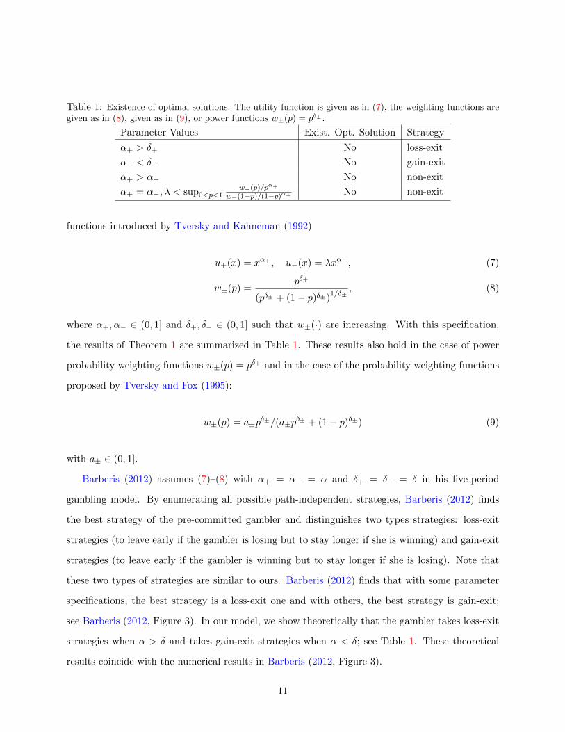
Table 1: Existence of optimal solutions. The utility function is given as in (7), the weighting functions aregiven as in (8), given as in (9), or power functions w±(p) = pδ± .

Parameter Values Exist. Opt. Solution Strategy

α+ > δ+ No loss-exit

α− < δ− No gain-exit

α+ > α− No non-exit

α+ = α−, λ < sup0<p<1w+(p)/pα+

w−(1−p)/(1−p)α+ No non-exit

functions introduced by Tversky and Kahneman (1992)

u+(x) = xα+ , u−(x) = λxα− , (7)

w±(p) =pδ±

(pδ± + (1− p)δ±)1/δ±

, (8)

where α+, α− ∈ (0, 1] and δ+, δ− ∈ (0, 1] such that w±(·) are increasing. With this specification,

the results of Theorem 1 are summarized in Table 1. These results also hold in the case of power

probability weighting functions w±(p) = pδ± and in the case of the probability weighting functions

proposed by Tversky and Fox (1995):

w±(p) = a±pδ±/(a±p

δ± + (1− p)δ±) (9)

with a± ∈ (0, 1].

Barberis (2012) assumes (7)–(8) with α+ = α− = α and δ+ = δ− = δ in his five-period

gambling model. By enumerating all possible path-independent strategies, Barberis (2012) finds

the best strategy of the pre-committed gambler and distinguishes two types strategies: loss-exit

strategies (to leave early if the gambler is losing but to stay longer if she is winning) and gain-exit

strategies (to leave early if the gambler is winning but to stay longer if she is losing). Note that

these two types of strategies are similar to ours. Barberis (2012) finds that with some parameter

specifications, the best strategy is a loss-exit one and with others, the best strategy is gain-exit;

see Barberis (2012, Figure 3). In our model, we show theoretically that the gambler takes loss-exit

strategies when α > δ and takes gain-exit strategies when α < δ; see Table 1. These theoretical

results coincide with the numerical results in Barberis (2012, Figure 3).

11

For the weighting function proposed by Prelec (1998)

w±(p) = e−a±(− ln p)δ± , (10)

with a± > 0 and δ± ∈ (0, 1], condition (4) is satisfied for any δ+ < 1 or for δ+ = 1 and α+ > a+.

In this case, the gambler takes an asymptotical loss-exit strategy. Condition (5), however, is not

satisfied for any δ− < 1.

4 Pre-committed Gamblers with Power Utility and Weighting

Functions

In this section, we solve problem (2) for a pre-committed gambler when the utility function is

piece-wise power and the probability weighting functions are power functions, i.e., when

u+(x) = xα+ , u−(x) = λxα− , w+(p) = pδ+ , w−(p) = pδ− (11)

with α± ∈ (0, 1], δ± ∈ (0, 1], and λ > 0. The parameters α+ and α− measure the diminishing

sensitivity of the utility of gains and losses, respectively; the smaller α+ and α− are, the more risk

averse regarding gains and the more seeking regarding losses the gambler is, respectively.

The parameter λ is related to loss aversion, a phenomenon that individuals are more sensitive

to losses than to gains; see for instance Kahneman et al. (1990). Various definitions of loss aversion

degree, a measure of the extent to which individuals are averse to losses, have been proposed in the

literature, including the definition u−(x)/u+(x), ∀x > 0 by Kahneman and Tversky (1979), that

u−(1)/u+(1) by Tversky and Kahneman (1992), that u′−(x)/u′+(x), ∀x > 0 by Wakker and Tversky

(1993), that limx↓0 u−(x)/u+(x) by Kobberling and Wakker (2005), and that limx↑+∞ u−(x)/u+(x)

by He and Zhou (2011). Save for the definition by Tversky and Kahneman (1992), the parameter λ

in (11) does not coincide with all the other definitions unless α+ = α−. In addition, the definition

of loss aversion degree by Tversky and Kahneman (1992) depends on the choice of the unit of

monetary payoffs; e.g., using dollars and euros as the unit lead to different loss aversion degree by

12

this definition. Therefore, λ, although related to loss aversion, can hardly be regarded as the loss

aversion degree. However, with α+ and α− being fixed, the larger λ is, the more loss averse and

hence the more overall risk averse the gambler is.

Note that a typical probability weighting function is inverse-S-shaped, i.e., is concave in its low

end and convex in its high end. The power probability weighting functions in (11), however, are

concave. We consider the power instead of inverse-S-shaped probability weighting functions for

two reasons. First, even with power probability weighting functions, the casino gambling problem

is extremely involved to solve. With a general inverse-S-shaped probability weighting function,

tractable solutions seems hardly possible. Secondly, two probability weighting functions in CPT

are used to model individuals’ tendency to overweight the tails of payoff distributions. For a mixed

gamble, i.e., a gamble with both possible gains and possible losses, the tails refer to significant

gains and losses of small probability, so such tendency is captured by the concave parts in the

low ends of the two probability weighting functions; see the CPT preference value (1). In our

gambling problem, the cumulative gain or loss represents a mixed gamble. As a result, the two

power probability weighting functions are able to capture the tendency to overweight the tails of

payoff distributions. We can see that the smaller δ+ and δ− are, the more the gambler overweighs

large gains and losses of small probability, respectively.

In the remainder of this section, we always assume (11) for the utility and probability weighting

functions. Because of the results in Table 1, we also assume α+ ≤ δ+, α− ≥ δ−, and α+ ≤ α−

throughout this section.

13

4.1 Infinite-Dimensional Programming

As shown in He et al. (2015), problem (1) is equivalent to the following infinite-dimensional opti-

mization problem

maxx,y

U(x,y)

subject to 1 ≥ x1 ≥ x2 ≥ ... ≥ xn ≥ ... ≥ 0,

1 ≥ y1 ≥ y2 ≥ ... ≥ yn ≥ ... ≥ 0,

x1 + y1 ≤ 1,∑∞n=1 xn =

∑∞n=1 yn,

(12)

where we denote x := (x1, x2, . . . ),y := (y1, y2, . . . ), and the objective function

U(x,y) :=∞∑n=1

(u+(n)− u+(n− 1))w+(xn)−∞∑n=1

(u−(n)− u−(n− 1))w−(yn)

with U(x,y) := −∞ if the second sum of infinite series is infinity. Here, x and y stand for the

decumulative distribution of the gain and the cumulative distribution of the loss, respectively, of Sτ

for some stopping time τ ; i.e., xn = P(Sτ ≥ n) and yn = P(Sτ ≤ −n), n ≥ 1. Once we solve (12) to

obtain distribution function of Sτ , we derive the optimal stopping time by Skorokhod embedding;

see He et al. (2015) for details.

Since S0 = 0, we can see that exit time τ = 0, which means not to gamble, corresponds to

x = y = 0, and the objective value U(x,y) = 0. Therefore, the gambler chooses to gamble if and

only if there exist x and y such that U(x,y) > 0.

4.2 Some Notations

Problem (12) is difficult to solve for two main reasons: First, the objective function is neither con-

cave nor convex in the decision variable because both w+(·) and w−(·) are concave. Secondly, there

are infinitely many constraints, so the standard Lagrange dual method is not directly applicable

even if the objective function were concave. After a detailed analysis, we are able to solve problem

14

(12) completely. The analysis is highly technical and involved, so we opt to present it in the online

appendix. Here, we only present the optimal solution. To this end, we need to introduce some

notations.

For any x and y of problem (12) corresponding to some stopping time τ , introduce s+ :=

(∑∞

n=2 xn)/x1 and s− := (∑∞

n=2 yn)/y1. Then,

s+ =

( ∞∑n=2

P(Sτ ≥ n)

)/P(Sτ ≥ 1) = E[Sτ − 1|Sτ ≥ 1].

Similarly, s− = E[−Sτ − 1|Sτ ≤ −1].

On the other hand, define z+ = (z+,1, z+,2, . . . ) with z+,n := xn+1/x1, n ≥ 1, and z− =

(z−,1, z−,2, . . . ) with z−,n := yn+1/x1, n ≥ 1. Note that∑∞

n=1 z±,n = s±.

In order to find the optimal x and y, we only need first to find the optimal z+ and z− with

constraint∑∞

n=1 z±,n = s±, and then to find the optimal x1, y1, and s±. Furthermore, s± imply

the conditional expected gain and loss of Sτ and the conditional-gain loss ratio; i.e.,

E[Sτ |Sτ ≥ 1] = s+ + 1, E[−Sτ |Sτ ≥ 1] = s− + 1, R(τ) =s+ + 1

s− + 1.

Therefore, the (asymptotically) optimal value s± will dictate whether the gambler takes a loss-exit,

gain-exit, or non-exit strategy. Finally, after we find optimal z±, x1, y1, and s±, we can compute

optimal x and y as x = (x1, x1z+) and y = (y1, y1z−), respectively.

Next, we present optimal z± given s± = s and the corresponding optimal value functions; the

details can be found in Propositions C.2 and C.4 of the online appendix. For each s > 0, define

z∗+(s) := (z∗+,1(s), z∗+,2(s), . . . ) and v+(s) as follows: If α+ ≤ δ+ = 1, define

z∗+,n(s) = 1, n = 1, . . . , bsc, z∗+,bsc+1 = s− bsc, z∗+,n = 0, n ≥ bsc+ 2, (13)

v+(s) = (1− (s− bsc))(bsc+ 1)α+ + (s− bsc)(bsc+ 2)α+ − 1. (14)

15

If α+ < δ+ < 1, define

z∗+,n(s) =

[µ(s)

((n+ 1)α+ − nα+

) 11−δ+

]∧ 1, n = 1, 2, . . . , (15)

v+(s) =∞∑n=1

{[µ(s)δ+

((n+ 1)α+ − nα+

) 11−δ+

]∧ [(n+ 1)α+ − nα+ ]

}, (16)

where µ(s) > 0 is the number such that∑∞

n=1 z∗+,n(s) = s.

Assume δ− ≤ α−. For each s > 0, define z∗−(s) := (z∗−,1(s), z∗−,2(s), . . . ) and v−(s) as follows:

Define B1 := 1. For each integer m ≥ 2, define Bm = m when α− = 1 and define Bm to be the

unique number in (m− 1,m) determined by

((m+ 1)α− − 1)

(Bmm

)δ−= (mα− − 1) + ((m+ 1)α− −mα−) (Bm −m+ 1)δ− (17)

when α− < 1. For s ∈ (m− 1, Bm], define

z∗−,n(s) = 1, n = 1, . . . ,m− 1, z∗−,m = s−m+ 1, z∗−,n = 0, n ≥ m+ 1, (18)

v−(s) = (mα− − 1) + ((m+ 1)α− −mα−)(s−m+ 1)δ− . (19)

For s ∈ (Bm,m], define

z∗−,n =s

m, n = 1, . . . ,m, z∗−,n = 0, n ≥ m+ 1, (20)

v−(s) = ((m+ 1)α− − 1)( sm

)δ−. (21)

Finally, for s = 0, define v+(s) = v−(s) = 0. The definition of z∗+(s) and z∗−(s) is irrelevant in

this case.

4.3 Optimal solution

Now, we are ready to present the optimal solution to problem (12) and compute its optimal value,

denoted as U∗. Recall that we assume α+ ≤ δ+, δ− ≤ α−, and α+ ≤ α−. The gambler does not

play in the casino if and only if the optimal solution to problem (12) is x∗ = y∗ = 0, and the

16

gambler chooses to play if and only if there exist x and y such that U(x,y) > 0.

Theorem 2 Assume α+ ≤ δ+, δ− ≤ α−, and α+ ≤ α−. Define

f(y, s+, s−) := (v+(s+) + 1)

(s− + 1

s+ + 1

)δ+yδ+ − λ(v−(s−) + 1)yδ− , y, s+, s− ≥ 0. (22)

(i) Suppose α+ = δ+ = α− = δ− = 1. If λ ≥ 1, the optimal solution to (12) is x∗ = y∗ = 0, i.e.,

the gambler does not play in the casino. If λ < 1, then U∗ =∞.

(ii) Suppose α+ = δ+ < 1. Then, U∗ = ∞ and there exist s+ > 0, x1 > 0, y, and z(n)+ , n ≥ 1

satisfying∑∞

i=1 z(n)+,i = s+ such that (x(n),y) with x(n) := (x1, x1z

(n)+ ) is feasible to problem

(12) and U(x(n),y) diverges to infinity as n→∞.

(iii) Suppose δ− ≤ δ+ and α+ < δ+. Define

M1 : = sups+≥0,s−≥0

[(v+(s+) + 1)(s− + 1)δ+

(v−(s−) + 1)(s+ + 1)δ−(s+ + s− + 2)δ+−δ−

],

M2 : = lim sups++s−→+∞

[(v+(s+) + 1)(s− + 1)δ+

(v−(s−) + 1)(s+ + 1)δ−(s+ + s− + 2)δ+−δ−

].

(23)

Then, 0 < M1 < +∞ and 0 ≤ M2 ≤ M1. Furthermore, M2 > 0 if and only if α− = α+

or α− = δ− and M2 = M1 if α− = δ−. When λ ≥ M1, the optimal solution to (12) is

x∗ = y∗ = 0, i.e., the gambler does not play in the casino, and when λ < M1, the gambler

plays in the casino. When M2 < λ < M1, U∗ < ∞ and the optimal solution exists and is

given as x∗ = (x∗1, x∗1z∗+(s∗+)), y∗ = (y∗1, y

∗1z∗−(s∗−)) where

(s∗+, s∗−) ∈ argmax

s+≥0,s−≥0f (y(s+, s−), s+, s−) , y(s+, s−) :=

s+ + 1

s+ + s− + 2,

y∗1 = y(s∗+, s∗−), x∗1 =

s∗− + 1

s∗+ + 1y∗1.

(24)

When λ < M2, the optimal solution does not exist, U∗ = +∞ if α+ = α− > δ− and U∗ < +∞

if α+ < α− = δ−, and there exist (s(n)+ , s

(n)− ) with limn→∞ s

(n)− = +∞ such that the objective

17

value of the pair x(n) := (x(n)1 , x

(n)1 z∗+(s

(n)+ )), y(n) := (y

(n)1 , y

(n)1 z∗−(s

(n)− )), where

y(n)1 :=

s(n)+ + 1

s(n)+ + s

(n)− + 2

, x(n)1 =

s(n)− + 1

s(n)+ + 1

y(n)1 , (25)

converges to U∗ as n → +∞. Moreover, s(n)+ /s

(n)− ’s converge to zero when α− = δ− and are

bounded from zero and from infinity when α− = α+ > δ−.

(iv) Suppose δ+ < δ− ≤ 1. Then, the gambler plays in the casino. When α− > δ−, U∗ < ∞ and

the optimal solution is x∗ = (x∗1, x∗1z∗+(s∗+)),y∗ = (y∗1, y

∗1z∗−(s∗−)) where

(s∗+, s∗−) ∈ argmax

s+≥0,s−≥0f (y(s+, s−), s+, s−) , y∗1 = y(s∗+, s

∗−), x∗1 =

s∗− + 1

s∗+ + 1y∗1,

y(s+, s−) := min

{(δ+(v+(s+) + 1)(s− + 1)δ+

δ−λ(v−(s) + 1)(s+ + 1)δ+

) 1δ−−δ+

,s+ + 1

s+ + s− + 2

}.

(26)

Moreover, if λ ≥M3, then we can take s∗− = 0 and

s∗+ = s1 :=∞∑n=1

((n+ 1)α+ − nα+)1

1−δ+ , M3 :=δ+

δ−(s1 + 2)δ−−δ+(s1 + 1)1−δ− . (27)

When α− = δ− and λ > M4, where

M4 :=δ+

δ−(s1 + 1)1−δ− < M3, (28)

the optimal solution exists and is given as (26) with s∗+ = s1 and s− = m for some nonnegative

integer m. If α− = δ− and λ ≤M4, then U∗ < +∞, the optimal solution does not exist, and

there exists s∗+ such that the objective value of the pair x(n) := (x(n)1 , x

(n)1 z∗+(s∗+)),y(n) :=

(y(n)1 , y

(n)1 z∗−(s

(n)− )) with s

(n)− = n, y

(n)1 :=

s∗++1

s∗++s(n)− +2

, x(n)1 =

s(n)− +1

s∗++1 y(n)1 converges to U∗ as

n→ +∞.

The proof of Theorem 2 is presented in Section C of the Online Appendix5.

Except for the case δ+ > α+ = α− > δ−, λ = M2 < M1 in which we do not know whether

5Available at http://ssrn.com/abstract=2682637 .

18

the optimal solution exists, we have solved problem (12) completely. When the optimal solution

exists, it is provided in closed form. Otherwise, a sequence of asymptotically optimal solutions are

provided.

In the case α+ = δ+ = α− = δ− = 1, the gambler does not play in the casino (i.e., the optimal

strategy is x∗ = y∗ = 0) when λ ≥ 1 and chooses to play (because the optimal value is infinite and

thus larger than the value of not gambling) when λ < 1.

In the case α+ = δ+ < 1, the optimal value is infinite. We find a sequence of asymptotically

optimal solutions (x(n),y). Note that the conditional expected gain is fixed to be s+ + 1 and the

conditional expected loss is also fixed. Thus, an infinite CPT value is achieved by taking strategies

that have fixed and finite conditional expected gain and loss.

In the case δ− ≤ δ+ and α+ < δ+, whether the optimal solution exists and whether the gambler

plays in the casino depend on λ. When λ ≥ M1, the gambler chooses not to play; otherwise she

plays. When M2 < λ < M1, the optimal solution exists. Finally, when λ < M2, , which can happen

only when α− = α+ or when α− = δ−, the optimal solution does not exist. In this case, a sequence

of asymptotically optimal solutions are given with s(n)− going to infinity and s

(n)+ /s

(n)− converging

to zero when α− = δ− or bounded from zero and from infinity when α− = α+ > δ−. Recall that

s(n)+ + 1 and s

(n)− + 1 stand for the conditional gain and loss, respectively. Therefore, when λ < M2,

the gambler takes a gain-exit strategy if α− = δ− and takes a non-exit strategy if α− = α+ > δ−.

In the case δ+ < δ− ≤ 1, the gambler plays in the casino. When α− > δ−, the optimal solution

exists, regardless of the value of λ. When α− = δ−, the optimal solution exists if and only if

λ > M4. When the optimal solution does not exist, a sequence of asymptotically optimal solutions

are given with s(n)+ to be fixed and s

(n)− going to infinity. Therefore, the gambler takes a gain-exit

strategy.

Finally, when the optimal solution exists, it must take the form x∗ = (x∗1, x∗1z∗+(s∗+)),y∗ =

(y∗1, y∗1z∗−(s∗−)) for some x∗1 ≥ 0, y∗1 ≥ 0, and s∗± ≥ 0. Moreover, s∗± can be solved by a two-

dimensional optimization problem (e.g., (24) and (26)).6 Recall z∗+(s) as defined in (13) and (15).

When δ+ = 1, z∗+,n(s) = 0 for n ≥ bsc+ 2, showing that the gambler plans to stop when reaching

6It is even possible to reduce it into a one-dimensional optimization problem which is easy to solve. We do notprovide details here because of space limit.

19

certain level of gains. When δ+ < 1, z∗+,n(s) > 0 for any n ≥ 1, showing that the gambler chooses

to continue with positive probabilities at any level of gains. On the other hand, recall z∗−(s) as

defined in (18) and (20). We can see that z∗−,n(s) = 0 for n ≥ dse + 1, showing that the gambler

plans to stop for sure when reaching certain level of losses. Furthermore, in the optimal solution

y∗ = (y∗1, y∗1z∗−(s∗−)), because y∗ is the cumulative distribution of the optimal strategy, the gambler

chooses to stop at no more than two loss levels (levels ds∗−e and ds∗−e + 1 when z∗−(s∗−) is in the

form (18) and levels 1 and ds∗−e+ 1 when z∗−(s∗−) is in the form (20)).

Table 2 summarizes the results in Theorems 1 and 2 regarding the solution to problem (12).

4.4 Examples

We consider two numerical examples to illustrate the optimal solution (x∗,y∗) to (12) and the

corresponding optimal strategy τ∗ of the pre-committed gambler. Denote {p∗n} as the optimal

distribution, i.e., the distribution of Sτ∗ . Obviously, p∗n = x∗n−x∗n+1, n ≥ 1, p∗−n = y∗n−y∗n+1, n ≥ 1.

Example 1 We set α+ = 0.5, α− = 0.9, δ± = 0.52, and λ = 2.25, which are reasonable values.7

According to Theorem 2, the optimal solution (12) exists: the optimal distribution is

p∗n =

0.1360(

(n0.5 − (n− 1)0.5)1/0.48 − ((n+ 1)0.5 − n0.5)1/0.48), n ≥ 2,

0.0933, n = 1,

0.8851, n = −1,

0, otherwise.

We construct a randomized, path-independent strategy τ∗ as in He et al. (2015) to achieve this

distribution: at each time t, given the gambler’s cumulative gain/loss level j, the gambler tosses a

random coin with the probability of the coin showing tails to be ri. If the coin shows heads, the

gambler continues; otherwise, the gambler stops. Using the explicit construction in He et al. (2015,

7This example is also reported in He et al. (2015).

20

Table 2: Optimal solution to problem (12) when the utility function is piece-wise power and theprobability weighting functions are power. The third column shows whether the gambler enters thecasino to gamble. The fourth column shows whether the optimal solution to problem (12) exists.The last column gives the optimal solution when it exists and the strategies (such as gain-exit, loss-exit, and non-exit strategies) the gambler takes when it does not. For the optimal solution, onlys∗+, s∗−, and y∗1 are listed. The optimal solution is then x∗ = (x∗1, x

∗1 ·z∗+(s∗+)),y∗ = (y∗1, y

∗1 ·z∗−(s∗−))

where x∗1 = (s∗− + 1)/(s∗+ + 1)y∗1 and z∗+(s) and z∗−(s) are given as in (13), (15), (18), and (20),respectively. The functions f , y, and y are given as in (22), (24), and (26), respectively. The blankcells indicate the only case in which problem (12) is not fully solved.

Gamb. Exist. Strategies

α+ = α− = λ ≥ 1 No Yes not gamble

δ+ = δ− = 1 λ < 1 Yes No non-exit

α+ > δ+ any λ Yes No loss-exit

α− < δ− any λ Yes No gain-exit

α− < α+ any λ Yes No non-exit

α+ = δ+ < 1 any λ Yes No certain asymptotical strategy

δ− ≤ δ+, λ ≥M1 No Yes not gamble

α+ < δ+, andλ < M1 Yes Yes

(s∗+, s∗−) ∈ argmaxf (y(s+, s−), s+, s−)

α− > max(α+, δ−) y∗1 = y(s∗+, s∗−)

δ− ≤ δ+, λ ≥M1 No Yes not gamble

α+ < δ+, andλ < M1 Yes No gain-exit

α− = δ− ≥ α+

λ ≥M1 No Yes not gamble

δ− ≤ δ+,M2 < λ < M1 Yes Yes

(s∗+, s∗−) ∈ argmaxf (y(s+, s−), s+, s−)

α+ < δ+, and y∗1 = y(s∗+, s∗−)

α− = α+ > δ− λ = M2 < M1 Yes

λ < M2 Yes No non-exit

α− > δ− > λ ≥M3 Yes Yes s∗+ = s1, s∗− = 0, and y∗1 = y(s∗+, s

∗−)

δ+ > α+ λ < M3 Yes Yes(s∗+, s

∗−) ∈ argmaxf(y(s+, s−), s+, s−)

and y∗1 = y(s∗+, s∗−)

α− = δ− >λ > M4 Yes Yes

s∗+ = s1, s∗− = m for some integer m

δ+ > α+ and y∗1 = y(s∗+, s∗−)

λ ≤M4 Yes No gain-exit

21

Appendix A.2), we obtain

rn = 1, n ≤ −1, r0 = 0, r1 = 0.0571, r2 = 0.0061, r3 = 0.0025, r4 = 0.0014, . . .

Therefore, the gambler’s strategy is as follows: stop once reaching −1; never stop at 0; toss a coin

with tails probability 0.0571 when reaching 1 and stop only if the toss outcome is tails; toss a coin

with tails probability 0.0061 when reaching 2 and stop only if the toss outcome is tails; and so on.

Example 2 To employ a randomized, path-independent strategy as in He et al. (2015), the gambler

needs to toss a random coin every time. Other types of randomized strategies are possible since

there can well be many different stopping times embedding the same stopped distribution. In

particular, we construct the so-called randomized Azema-Yor (AY) strategies in Appendix B. The

gambler needs less random coins to follow a randomized AY strategy than to use a randomized

path-independent strategy, at the cost of having to be path-dependent. We use an example to

compare the randomized path-independent and randomized AY strategies. To this end, we set

α+ = 0.6, δ+ = 0.7, α− = 0.8, δ− = 0.7, and λ = 1.05.8 We solve (12) to get the optimal

distribution

p∗n =

0.4465× ((n0.6 − (n− 1)0.6)1/0.3 − ((n+ 1)0.6 − n0.6)1/0.3), n ≥ 2,

0.3297, n = 1,

0.6216, n = −1,

0, otherwise.

(29)

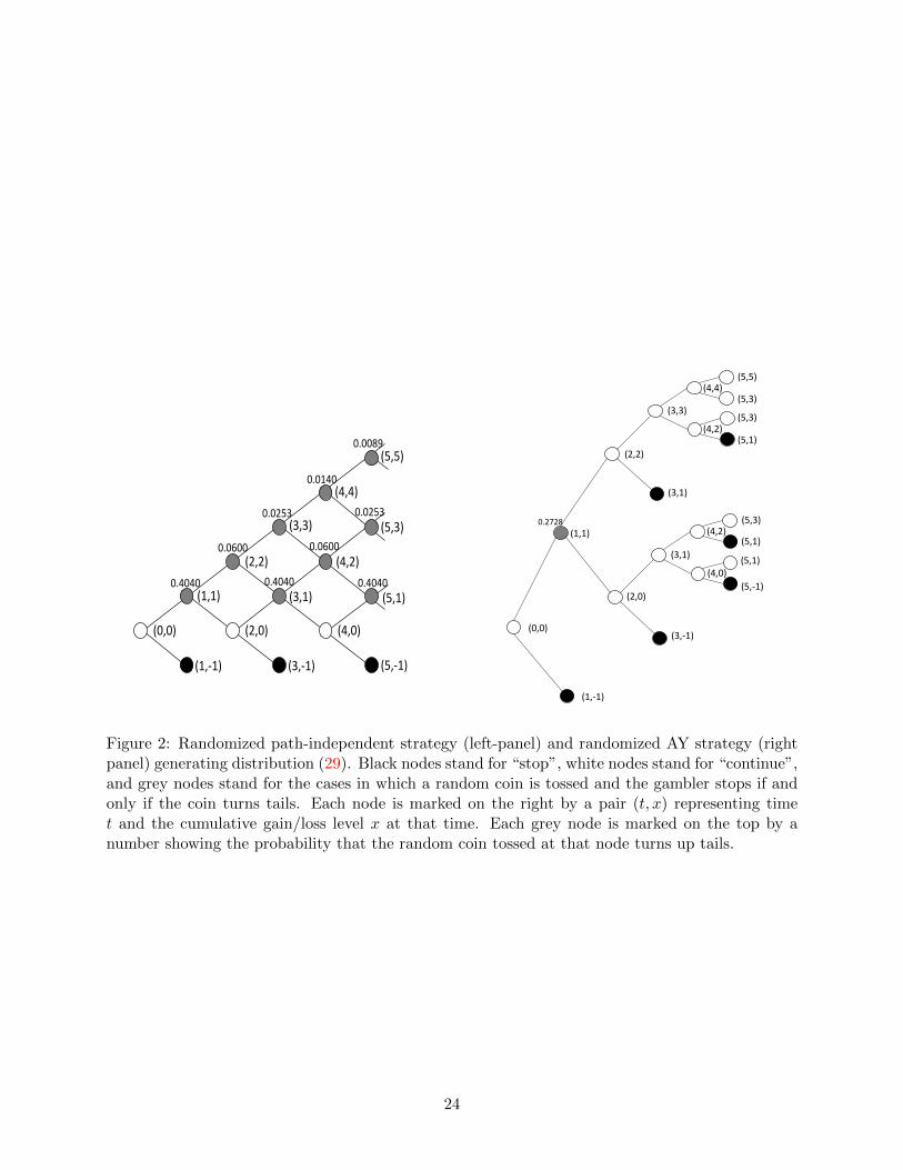
Figure 2 illustrates the randomized path-independent strategy as constructed in He et al. (2015)

and the randomized AY strategy as constructed in Appendix B of the present paper that lead to

the same optimal distribution {p∗n}. For the randomized path-independent strategy (left panel),

black nodes stand for “stop”, white nodes stand for “continue”, and grey nodes stand for the cases

in which a random coin is tossed and the gambler stops if and only if the coin turns tails. The

8For illustrative purpose, we use different parameter values from Example 1.

22

probability that the random coin turns tails is computed following the construction in He et al.

(2015), and the probability is shown on the top of each grey node. This strategy is path-independent

since the tail probability of the coin at each node depends only on the cumulative gain/loss level at

that node. However, to implement this path-independent randomized strategy, the gambler needs

to toss random coins most of the times; see the left panel of Figure 2.9

The right panel of Figure 2 illustrates the randomized AY strategy. Again, black nodes stand for

“stop”, white nodes stand for “continue”, and grey nodes stand for the cases in which a random coin

is tossed and the gambler stops if and only if the coin turns tails. The probability that the random

coin turns tails is computed following the construction given in Appendix B of the present paper

and is shown on the top of each grey node. We can see that this strategy is path-dependent. For

instance, consider time 3 and cumulative gain/loss level 1. If the gambler reaches this node along

the path from (0,0), through (1,1) and (2,2), and to (3,1), then she stops. If the gambler reaches

this node along the path from (0,0), through (1,1) and (2,0), and to (3,1), then she continues. This

exhibits a feature of the so-called “trailing stop-loss” strategy in stock trading, one that stops loss

at a percentage below a moving target (which can be the market price or the historical high): One

exits at (3,1) from (2.2) simply because it is a stop loss from the historical high. The continuation

at (3,1) from (2,0) is based on the symmetric idea. On the other hand, we can see that in the first

six periods, the gambler needs to use at most one random coin; i.e., there is only one grey node

in the right panel of Figure 2. Therefore, compared to the randomized independent strategy, the

randomized AY strategy involves less randomization at the cost of being path-dependent.

5 Naive Gamblers

Barberis (2012) finds in his five-period casino gambling model that, due to the probability weighting,

if the gambler revisits the gambling problem with the same CPT preferences in the future, she may

find the initial strategy decided at time 0 is no longer optimal. As a result, if she cannot commit

herself to following the initial strategy, she may change to a new strategy that can be totally

different from the initial one. Such type of gamblers are called naive gamblers.

9Black and white nodes are special cases where the tail probabilities of the coins turn out to be 1 and 0 respectively.

23

(1,1)

(1,-1) (3,-1) (5,-1)

0.4040 0.4040

0.0600 0.0600

0.0253 0.0253

0.0140

0.0089

(3,1) (5,1)

(2,2)

(3,3)

(4,4)

(0,0)

(5,3)

(5,5)

(4,2)

(2,0) (4,0)

0.4040

(1,1)

(3,1)

(3,-1)

(5,1)

(5,1)

(5,-1) (2,0)

(2,2)

(5,1) (3,1)

(4,2)

(4,0)

(5,3)

(5,3) (3,3)

(4,4)

(4,2)

(5,3)

(5,5)

(0,0)

(1,-1)

0.2728

Figure 2: Randomized path-independent strategy (left-panel) and randomized AY strategy (rightpanel) generating distribution (29). Black nodes stand for “stop”, white nodes stand for “continue”,and grey nodes stand for the cases in which a random coin is tossed and the gambler stops if andonly if the coin turns tails. Each node is marked on the right by a pair (t, x) representing timet and the cumulative gain/loss level x at that time. Each grey node is marked on the top by anumber showing the probability that the random coin tossed at that node turns up tails.

24

Formally, suppose now after T rounds of play, at time T the gambler has arrived at some node

and has not stopped yet with accumulated gain/loss equal to H. A naive gambler will re-consider

the choice between continuing and leaving at that node. Following Barberis (2012), we assume the

reference point in the CPT preference of the gambler at any time to be the initial wealth level.

As a result, the cumulative gain or loss of the gambler at any time n ≥ T is Sn. Conditioning on

ST = H, the gambling problem faced by the naive gambler is

maxτ∈TT,H VT,H(Sτ ) (30)

where TT,H := {τ ≥ T |τ ∈ AC and {(Sτ∧t − ST ) : t ≥ T} is uniformly integrable} and

VT,H(Sτ ) =∞∑n=1

u+(n)(w+(P(Sτ ≥ n|ST = H))− w+(P(Sτ > n|ST = H))

)−∞∑n=1

u−(n)(w−(P(Sτ ≤ −n|ST = H))− w−(P(Sτ < −n|ST = H))

),

where, as before, VT,H(Sτ ) := −∞ if the second sum of infinite series is infinite. One can see that

the CPT value of the strategy of leaving the casino at T is u(H) := u+(H)1H≥0 − u−(H)1H<0.

As a result, the naive gambler decides to play at time T with cumulative gain/loss level H if and

only if the optimal value of problem (30) is strictly larger than u(H). Mathematically, (30) can be

solved using exactly the same method for solving problem (2).

The following theorem is parallel to Theorem 1, and the proof is omitted. For two integers

b < 0 < a, we denote the relative first exit time after T by

τTa,b := inf{n ≥ T : Sn − ST = a or Sn − ST = b}.

Theorem 3 Fix time T > 0 and level H, −T ≤ H ≤ T . Let V ∗T,H denote the value of the

optimization problem (30).

(i) Suppose (4) holds. Then, V ∗T,H =∞ and there exists b < 0 such that lima→+∞ VT,H(SτTa,b) =

+∞.

25

(ii) Suppose (5) holds. Then, V ∗T,H = supx≥0 u+(x). Moreover, the optimal solution to problem

(30) does not exist and VT,H(SτTa,b) with a = bkε/(1+ε)c and b = −k converges to V ∗T,H as k

goes to infinity.

(iii) Assume limx→+∞ u+(x) = +∞ and suppose condition (6) holds. Then, V ∗T,H =∞ and there

exists c > 0 such that limk→+∞ VT,H(SτTa,b) = +∞ where a = dcke and b = −k.

Theorem 3 shows that when one of the conditions (4)–(6) is satisfied, the naive gambler, who

adjusts her optimal strategy after each bet, always finds continue gambling more attractive. So

in effect, she never stops gambling. In addition, this is true even when we restrict the gambler to

simple exit strategies τTa,b, which are in particular path-independent.

With piece-wise power utility function (7) and weighting functions (8), or weighting functions

(9), or power weighting functions w±(p) = pδ± , the naive gambler never stops gambling if one of

the conditions in Table 1 is satisfied. For weighting functions (10), the naive gambler never stops

gambling if δ+ < 1 or if δ+ = 1 and α+ > a+.

Ebert and Strack (2012) also study the conditions under which a naive gambler does not stop

gambling. They assume the naive gambler can construct strategies with arbitrarily small random

payoffs and then show that the naive gambler prefers skewness in the small and thus does not stop

gambling. Recently, in a stylized continuous-time example10, Henderson et al. (2015) employ the

methodology of Xu and Zhou (2012) to obtain analytically the optimal strategy of a pre-committed

gambler. They then use it to study actual optimal behaviours of a naive gambler. They show that

if a naive gambler is allowed to used randomized strategies and prefers to use “natural” strategies

that are time-homogeneous and Markovian, he/she may stop instantly with a positive probability

or even for sure.

We note that our approach to comparing pre-committed and naive gamblers is similar in spirit

to Henderson et al. (2015). However, in our model, the naive gambler cannot construct strategies

with arbitrarily small random payoffs because the stake size is fixed at $1. Consequently, the

results in Ebert and Strack (2012) and Henderson et al. (2015) do not apply in our setting. In

fact, here we show that the naive gambler prefers skewness in the large. Indeed, in Theorem 3, for

10More elaborate setting with a geometric Brownian motion and CPT preferences is addressed numerically.

26

stopping time τTa,b we send either a, or b, or both to infinity, and thus the payoff of τTa,b can be very

large.11 The following result compares the optimal strategy of the pre-committed gambler and the

actual behavior of the naive gambler when the utility function is given as in (7) and the weighting

functions are w±(p) = pδ± .

Theorem 4 (i) Assume δ+ < 1. For any H ≥ 1, there exists feasible (x,y) to problem (30)

such that U(x,y) > Hα+.

(ii) Assume δ+ < δ−. Then, for any H ≤ −1, there exists feasible (x,y) to problem (30) such

that U(x,y) > −λ(−H)α−.

The proof of Theorem 4 is provided in Section D.1 of the Online Appendix.

Theorem 4-(i) shows that the naive gambler continues with a positive probability at any gain

level, which is the same as a pre-committed gambler. On the other hand, Theorem 4-(ii) indicates

that if δ+ < δ−, at each time, with a positive probability the naive gambler does not stop. More

precisely, either she simply continues, or else she might want to toss a coin to decide whether to

continue to play or not. In particular, if α+ < δ+ < δ− < α−, according to Theorem 2, the

pre-committed gambler stops for sure if the loss hits certain level. In sharp contrast, the naive

gambler’s actual behavior is to play with a positive probability at any loss level.

The reason why the naive gambler behaves differently from the pre-committed gambler is the

same as explained in Barberis (2012): at time 0, the pre-committed gambler decides to stop when

the loss reaches certain level, e.g., L, in the future because the probability of having losses strictly

larger than L is small from time 0’s perspective and this small probability is exaggerated due to

probability weighting. For the naive gambler, when she actually reaches loss level L at some time

t, the probability of having losses strictly larger than L is no longer small from time t’s perspective.

Consequently, loss L is not overweighted by the naive gambler at time t, so she chooses to take a

chance and not to stop gambling.

Finally, we provide a numerical example to show the actual behavior of the naive gambler.

11In Appendix W2 of Ebert and Strack (2012), the authors also consider preference for skewness in the large whenthe utility function is piece-wise power.

27

Table 3: Optimal solution p∗H,n to (30) for H = ±1,±2, . . . ,±5. Denote qn =(n0.5 − (n − 1)0.5

)1/0.48 −((n+ 1)0.5 − n0.5

)1/0.48, n ≥ 1.

H n ≤ −7 −6 −5 −4 −3 −2 −1 0 1 2 n ≥ 3

−5 0 0.977 0 0 0 0 0 0 0 0.0096 0.1477qn

−4 0 0 0.971 0 0 0 0 0 0.0063 0.1453qn 0.1453qn

−3 0 0 0 0.961 0 0 0 0 0.0161 0.1424qn 0.1424qn

−2 0 0 0 0 0.947 0 0 0 0.0308 0.1393qn 0.1393qn

−1 0 0 0 0 0 0.924 0 0 0.0543 0.1364qn 0.1364qn

0 0 0 0 0 0 0 0.885 0 0.0933 0.1360qn 0.1360qn

1 0 0 0 0 0 0 0 0.850 0.1501qn 0.1501qn 0.1501qn

2 0 0 0 0 0 0 0 0.700 0.3003qn 0.3003qn 0.3003qn

3 0 0 0 0 0 0 0 0.550 0.4504qn 0.4504qn 0.4504qn

4 0 0 0 0 0 0 0 0.400 0.6006qn 0.6006qn 0.6006qn

5 0 0 0 0 0 0 0 0.250 0.7507qn 0.7507qn 0.7507qn

Example 3 We use the same parameter values as in Example 1. We compute the optimal solution

to (30) for H = ±1,±2, . . . ,±5 to illustrate the actual behavior of the naive gambler. The details of

how to find the solution are provided in Section D.2 of the online appendix. The optimal solutions

p∗H,n, n ∈ Z, H = ±1,±2, . . . ,±5 are shown in Table 3, where qn :=(n0.5− (n− 1)0.5

)1/0.48−((n+

1)0.5 − n0.5)1/0.48

, n ≥ 1.

We can see that for H ≤ −1, p∗H,H = 0, indicating that the naive gambler will play for sure at

any loss level. This strategy is in contrast to the optimal strategy of the pre-committed gambler

shown in Example 1: stop once the loss accumulates to $1. On the other hand, for H ≥ 1,

p∗H,H ∈ (0, 1), indicating that the naive gambler will play with some probability at any gain level.

We remark that the discussion in this section has been based on the assumption that the gambler

does not change the reference point, an assumption also used in Barberis (2012). An alternative

model is one in which the gambler adjusts the reference point endogenously for prior gains and

losses. This promises to be a entirely different and difficult problem, which is left for future study.

6 Conclusion

In this paper, we have solved the casino gambling problem proposed by He et al. (2015) for a

pre-committed gambler and a naive gambler. The pre-committed gambler is offered a fair bet

28

repeatedly, decides at time 0 when to leave the casino, and commits herself to this strategy in the

future. The naive gambler is offered the same bet repeatedly, decides at each time when to leave

the casino, but fails to commit herself in the future.

We have found the conditions under which the pre-committed gambler takes (essentially) loss-

exit (namely stop-loss), gain-exit (corresponding to disposition effect), and non-exit strategies and

our theoretical results are consistent with the numerical results in Barberis (2012). When the utility

function is piece-wise power and the probability weighting functions are power, we have derived the

optimal strategy of the pre-committed gambler completely and analytically by solving an infinite

dimensional program. We have found that the optimal strategy of the pre-committed gambler,

when exists, is to cap the loss, i.e., to stop before the loss hits a certain level.

We have also revealed that, under some conditions, the optimal strategy of the pre-committed

gambler and the actual strategy implemented by the naive gambler are totally different: the pre-

committed gambler must stop if her cumulative loss reaches a certain level whereas the naive

gambler continues to play with a positive probability at any loss level.

A Proof of Theorem 1

(i) It is well known that

P(Sτa,b = a) =−ba− b

, P(Sτa,b = b) =a

a− b, P(Sτa,b = n) = 0, n /∈ {a, b}.

Consequently,

V (Sτa,b) = u+(a)w+

(−ba− b

)− u−(−b)w−

(a

a− b

)= u+(−b(x− 1))w+ (1/x)− u−(−b)w− (1− 1/x)

29

where x := (a − b)/(−b). Choose b ∈ Z such that −b ≥ 2s. Then, −b(x − 1) ≥ sx for any

x ≥ 2. Consequently, as a→ +∞, we have x→ +∞ and

V (Sτa,b) ≥ u+(sx)w+ (1/x)− u−(−b)w− (1− 1/x)→ +∞.

(ii) We have

V (Sτa,b) = u+(a)w+

(−ba− b

)− u−(−b)w−

(a

a− b

)= u+

(bkε/(1+ε)c

)w+ (1− 1/y)− u−(k)w− (1/y)

where y := (a− b)/a. We can see that

y = 1 +−ba

= 1 +k

bkε/(1+ε)c>

k

kε/(1+ε)= k1/(1+ε).

As a result,

lim supk→+∞

u−(k)w− (1/y) ≤ lim supk→+∞

u−(k)w−

(1/k1/(1+ε)

)= 0.

In addition, as k → +∞, we have w+ (1− 1/y) goes to 1. Consequently, limk→+∞ V (Sτa,b) =

supx>0 u+(x). On the other hand, it is straightforward to see that for any feasible τ , V (Sτ ) <

supx>0 u+(x). Therefore, problem (2) is ill-posed and the optimal value is supx>0 u+(x).

(iii) Suppose lim supx→+∞u−

(p0

1−p0x)

u+(x) < w+(p0)w−(1−p0) for some p0 ∈ (0, 1). Then, there exists δ0 > 0

and ε0 > 0 such that

w+(p)

w−(1− p)> lim sup

x→+∞

u−

(p0

1−p0x)

u+(x)+ ε0, ∀p ∈ [p0 − δ0, p0 + δ0].

Choose c > 0 such that 1/(1 + c) = p0. Then, for sufficiently large k, we have k/(dcke+ k) ∈

30

[p0 − δ0, p0 + δ0]. Consequently, as k goes to +∞,

V (Sτa,b) = u+ (dcke)w+

(k

dcke+ k

)− u− (k)w−

(dckedcke+ k

)

= u+ (dcke)w−(dckedcke+ k

)w+

(k

dcke+k

)w−

(dckedcke+k

) − u− (k)

u+ (dcke)

≥ u+ (dcke)w− (1− (p0 + δ0))

w+

(k

dcke+k

)w−

(dckedcke+k

) − u− (k)

u+ (ck)

= u+ (dcke)w− (1− (p0 + δ0))

w+

(k

dcke+k

)w−

(dckedcke+k

) − u− (k)

u+

(1−p0

p0k)

≥ u+ (dcke)w− (1− (p0 + δ0)) ε0 → +∞.

B AY-like Stopping Times: Exit for Large Relative Loss

In this section, we consider strategies combining path-dependence and randomization, which are

randomization of the Azema-Yor stopping time in continuous-time Skorokhod embedding problems.

Suppose we want to construct a stopping time τ so that Sτ follows distribution µ. Recall that

{St} is the symmetric random walk. Denote x := sup{n ∈ Z|µ({n}) > 0} and x := inf{n ∈

Z|µ({n} > 0}. Consider a countable sequence of integers 0 ≥ x01 > x0

2 > . . . and ρ0i ∈ [0, 1], i ≥ 1 if

x = −∞ and a finite sequence of integers 0 ≥ x01 > x0

2 > · · · > x0m0+1 and ρ0

i ∈ [0, 1], i = 1, . . . ,m0

if x > −∞. For each integer n ∈ [1, x), consider a sequence of integers: n ≥ xn1 > xn2 > · · · > xnmn+1

and ρni ∈ [0, 1], i = 1, . . .mn.

Given xni ’s and ρni ’s, construct the following stopping time: For each integer n ∈ [0, x), at the

first time when St = n, consider the hitting time of {St} to two levels xn1 and n+ 1. If St hits xn1

first, then an independent coin with tails probability ρn1 is tossed, and one stops when the outcome

is tails. Otherwise, continue and consider the hitting time of {St} to two levels xn2 and n + 1. If

{St} hits xn2 first, then an independent coin with tails probability ρn2 is tossed, and one stops when

the outcome is tails. Continue the strategy until one stops at xni for some i = 1, . . . ,mn, or {St}

hits xnmn+1 in which case one stops for sure, or {St} hits n + 1 in which case a new maximum is

31

hit. Finally, at the first time St hits x, stop.

The stopping time constructed above is called randomized Azema-Yor stopping time. Note

that xni , i = 1, . . . ,mn + 1 and ρni , i = 1, . . . ,mn, n ≥ 0 are part of the randomized Azema-Yor

stopping time. Intuitively, following an Azema-Yor stopping time, the gambler stops with possibly

randomization when her maximum drawdown, which is the loss accumulated since the time when

the historical maximum is reached, hits certain level.

Theorem 5 For any µ ∈M0(Z) as defined in (3), there exists a randomized Azema-Yor stopping

time τ such that Sτ has the same distribution as µ. Moreover {Sτ∧t} is uniformly integrable and

never visits the states outside any interval that contains the support of µ.

Proof We assume µ 6= 0 to exclude the trivial case. Because the mean of µ is zero, µ must have

positive probability mass on some positive integers. Define the barycenter function associated with

µ:

ψµ(x) =1∑

n≥x µ({n})∑n≥x

nµ({n}), x ∈ R.

Denote x := sup{n ∈ Z|µ({n}) > 0}, which can either be a positive integer or be +∞, and define

ψµ(x) = +∞ for x > x. It is clear that ψµ(x) is left-continuous, increasing, and finite-valued

on (−∞, x] ∩ R. Furthermore, limx↓−∞ ψµ(x) = 0 because the mean of µ is zero. In addition,

y := sup{ψµ(x)|ψµ(x) < +∞} is finite if and only if x < +∞, in which case y = ψµ(x) = x.

Define bµ as the right-continuous inverse of ψµ, i.e.,

bµ(y) := sup{x|ψµ(x) ≤ y}, y ≥ 0.

Then, bµ is increasing, right-continuous, and integer valued on (0,+∞). Moreover, bµ(0) > −∞ if

and only if µ((−∞, n]) = 0 for some n ∈ Z, in which case bµ(0) is an integer and bµ(y) is continuous

at y = 0. Furthermore, bµ(y) = x if and only if y ≥ y.

Several properties of bµ and ψµ are needed in the following proof: First, ψµ(x) > x except for

x = x < +∞. Second, bµ(y) < y except for y = y = ψµ(x) = x < +∞. Third, ψµ(bµ(y)) ≤ y for

32

any y ≥ 0 (with ψµ(−∞) := 0) and bµ(ψµ(x)) ≥ x for any x < x. Fourth, ψµ(bµ(y)+) > y for any

y < y. Fifth, for any integer y, µ({y}) = 0 if and only if y is not in the range of bµ.

In the following, we determine xni , i = 1, . . . ,mn + 1 and ρni , i = 1, . . . ,mn, n ≥ 0 so that the

corresponding randomized Azema-Yor stopping time leads to distribution µ.

For each 1 ≤ n < x, rank {bµ(y)|y ∈ [n, n+1]}∩(−∞, n], which is a set of finitely many integers,

as xn1 > xn2 > · · · > xnmn+1. Rank {bµ(y)|y ∈ [0, 1]} ∩ (−∞, 0], which is a set of finitely many

integers x01 > x0

2 > . . . x0m0+1 if bµ(0) > −∞ and a set of countably many integers x0

1 > x02 > . . .

otherwise. By definition, xnmn+1 = bµ(n) for each 1 ≤ n < x. In addition, because bµ(y) < y unless

y = y = ψµ(x) = x < +∞, we conclude that for each 1 ≤ n < x, bµ(n) ≤ n − 1 and consequently

xn−11 = bµ(n) = xnmn+1.

In the following, we construct ρni ’s so that the corresponding randomized Azema-Yor stopping

time τ leads to distribution µ. Denote Hj = inf{t ≥ 0 : St ≥ j}, for each integer j ≥ 0. Denote

µ(x) := µ([x,+∞)), x ∈ R. By constructing ρni ’s, we show that τ satisfies

P(Sτ = y and τ < Hj+1) = µ({y}), for y < xj1

P(Sτ = y and τ < Hj+1) = µ(xj1)j+1−ψµ(xj1)

j+1−xj1, for y = xj1

P(Sτ = y and τ < Hj+1) = 0, for y > xj1,

(31)

for any 0 ≤ j < x.

We use mathematical induction to show that (31) holds for any 0 ≤ j < x. To this end, we need

to show (i) (31) holds for j = 0 and (ii) (31) holds for j = n < x if it holds for j = 0, . . . , n− 1.

We prove part (ii) first; i.e., we prove (31) holds for j = n < x given that it holds for j =

0, . . . , n− 1. Because (31) is true for j = n− 1, we obtain

P(τ ≥ Hn) = 1− P(τ < Hn) = 1−

∑y<xn−1

1

µ({y})

− µ(xn−11 )

n− ψµ(xn−11 )

n− xn−11

= µ(xn−11 )− µ(xn−1

1 )n− ψµ(xn−1

1 )

n− xn−11

= µ(xn−11 )

ψµ(xn−11 )− xn−1

1

n− xn−11

.

33

Because ψµ(x) > x except for x = x < +∞ and xn−11 = bµ(n) ≤ n − 1 < x, we conclude that

P(τ ≥ Hn) > 0.

Now, we consider the case in which mn = 0. In this case, xn1 = xnmn+1 = xn−11 . By the

construction of τ , after Hn, one stops for sure at the first time when hitting xn1 before hitting n+1.

Consequently,

P(Sτ = xn1 , τ < Hn+1)

=P(Sτ = xn1 , τ < Hn) + P(Sτ = xn1 , τ < Hn+1|τ ≥ Hn) · P(τ ≥ Hn)

=P(Sτ = xn−11 , τ < Hn) +

1

n+ 1− xn1· µ(xn−1

1 )ψµ(xn−1

1 )− xn−11

n− xn−11

=µ(xn−11 )

n− ψµ(xn−11 )

n− xn−11

+1

n+ 1− xn1· µ(xn−1

1 )ψµ(xn−1

1 )− xn−11

n− xn−11

=µ(xn1 )n− ψµ(xn1 )

n− xn1+

1

n+ 1− xn1· µ(xn1 )

ψµ(xn1 )− xn1n− xn1

=µ(xn1 )n+ 1− ψµ(xn1 )

n+ 1− xn1.

Therefore, (31) holds for j = n.

Next, we consider the case in which mn ≥ 1. Note that xnmn+1 = bµ(n) < n because n < x.

Define

gk : =n+ 1− xnkP(τ ≥ Hn)

µ({xnk}), k = 2, 3, . . . ,mn,

gmn+1 : =n+ 1− xnmn+1

P(τ ≥ Hn)

[µ({xnmn+1})− µ(xnmn+1)

n− ψµ(xnmn+1)

n− xnmn+1

],

fmn+1 : = 0, fk = fk+1 + gk+1, k = 1, 2, . . . ,mn.

34

Straightforward calculation leads to

µ({xnmn+1})− µ(xnmn+1)n− ψµ(xnmn+1)

n− xnmn+1

=1

n− xnmn+1

∑y>xnmn+1

yµ({y})− nµ((xnmn+1,+∞))

=µ((xnmn+1,+∞))

n− xnmn+1

[ψµ(xnmn+1+)− n

]=µ((xnmn+1,+∞))

n− xnmn+1

[ψµ(bµ(n)+)− n] > 0

where the inequality is the case because xnmn+1 = bµ(n) < n < x and ψµ(bµ(y)+) > y for any y < y.

Consequently, gmn+1 > 0. On the other hand, because µ({y}) = 0 for any y that is not in the range

of bµ, we conclude that

mn+1∑k=2

(n+ 1− xnk)µ({xnk}) =∑

xnmn+1≤y<xn1

(n+ 1− y)µ({y})

=(n+ 1)(µ(xnmn+1)− µ(xn1 ))−[ψµ(xnmn+1)µ(xnmn+1)− ψµ(xn1 )µ(xn1 )

]=(n+ 1− ψµ(xnmn+1))µ(xnmn+1)− (n+ 1− ψµ(xn1 ))µ(xn1 ).

Consequently, we have

f1 =

mn+1∑k=2

gk =1

P(τ ≥ Hn)

[mn+1∑k=2

(n+ 1− xnk)µ({xnk})− (n+ 1− xnmn+1)µ(xnmn+1)n− ψµ(xnmn+1)

n− xnmn+1

]

=1

P(τ ≥ Hn)

[µ(xnmn+1)

ψµ(xnmn+1)− xnmn+1

n− xnmn+1

− (n+ 1− ψµ(xn1 ))µ(xn1 )

]=1− (n+ 1− ψµ(xn1 ))µ(xn1 )

P(τ ≥ Hn)≤ 1,

where the inequality is the case because ψµ(xn1 ) = ψµ(bµ(n+1)) ≤ n+1. Therefore, fk is decreasing

in k = 1, 2, . . . ,mn, fmn > 0 and f1 ≤ 1.

Define ρnk := 1−(fk/fk−1), k = 1, . . . ,mn where f0 := 1. Denote ρnmn+1 := 1 = 1−(fmn+1/fmn)

35

and xn0 := n. Then, for each k = 1, . . . ,mn + 1,

P(Sτ = xnk ,Hn ≤ τ < Hn+1)

=P(Sτ = xnk , τ < Hn+1|τ ≥ Hn) · P(τ ≥ Hn)

=

k−1∏j=1

(n+ 1− xnj−1

n+ 1− xnj(1− ρnj )

) n+ 1− xnk−1

n+ 1− xnkρnkP(τ ≥ Hn)

=1

n+ 1− xnk

k−1∏j=1

(1− ρnj )

ρnkP(τ ≥ Hn)

=1

n+ 1− xnk(fk−1 − fk)P(τ ≥ Hn).

Therefore, for k = 2, . . . ,mn, we have P(Sτ = xnk ,Hn ≤ τ < Hn+1) = µ({xnk}). For k = mn + 1, we

have P(Sτ = xnmn+1,Hn ≤ τ < Hn+1) = µ({xnmn+1}) − µ(xnmn+1)n−ψµ(xnmn+1)

n−xnmn+1. For k = 1, we have

P(Sτ = xn1 ,Hn ≤ τ < Hn+1) =n+1−ψµ(xn1 )n+1−xn1

µ(xn1 ).

Because xnmn+1 = xn−11 and (31) holds for j = 0, . . . , n− 1, we conclude that for y < xnmn+1,

P(Sτ = y, τ < Hn+1) = P(Sτ = y, τ < Hn) + P(Sτ = y,Hn ≤ τ < Hn+1)

= P(Sτ = y, τ < Hn) = µ({y}).

For y = xnk , k = 2, 3, . . . ,mn, we have

P(Sτ = xnk , τ < Hn+1) = P(Sτ = xnk , τ < Hn) + P(Sτ = xnk ,Hn ≤ τ < Hn+1)

= P(Sτ = xnk ,Hn ≤ τ < Hn+1) = µ({xnk}).

For y = xnmn+1 = xn−11 , we have

P(Sτ = xnmn+1, τ < Hn+1) = P(Sτ = xnmn+1, τ < Hn) + P(Sτ = xnmn+1,Hn ≤ τ < Hn+1)

= P(Sτ = xn−11 , τ < Hn) + P(Sτ = xnmn+1,Hn ≤ τ < Hn+1)

= µ({xnmn+1}).

36

For y = xn1 , we have

P(Sτ = xnk , τ < Hn+1) = P(Sτ = xnk , τ < Hn) + P(Sτ = xnk ,Hn ≤ τ < Hn+1)

= P(Sτ = xnk ,Hn ≤ τ < Hn+1) =n+ 1− ψµ(xn1 )

n+ 1− xn1µ(xn1 ).

For y ∈ [xnmn+1, xn1 ] but not being any of xni , i = 1, . . . ,mn + 1, it is not in the range of bµ.

Consequently, µ({y}) = 0, and thus

P(Sτ = y, τ < Hn+1) = P(Sτ = y, τ < Hn) + P(Sτ = y,Hn ≤ τ < Hn+1)

= P(Sτ = y,Hn ≤ τ < Hn+1) = 0 = µ({y}).

Finally, for y > xn1 , by construction, we have

P(Sτ = y, τ < Hn+1) = P(Sτ = y, τ < Hn) + P(Sτ = y,Hn ≤ τ < Hn+1) = 0.

Therefore, (31) holds for j = n.

Next, we prove part (i) of the mathematical induction; i.e., we prove (31) holds for j = 0. When

x0i ’s are finitely many, the proof is exactly the same as the proof of part (ii) of the mathematical

induction. When x0i ’s are countably many, we define

gk =1− x0

k

P(τ ≥ H0)µ({x0

k}) = (1− x0k)µ({x0

k}), k ≥ 2, fk =∞∑

i=k+1

gi, k ≥ 1.

Note that x0k ≤ x0

1 ≤ 0, so gk’s are positive. Furthermore, because µ({y}) = 0 for any y that is not

in the range of bµ, we conclude that

∞∑k=2

gk =

∞∑k=2

(1− x0k)µ({x0

k}) =∑y<x0

1

(1− y)µ({y}) = 1− µ(x01)−

∑y<x0

1

yµ({y})

= 1− µ(x01) +

∑y≥x0

1

yµ({y}) = 1− µ(x01)(1− ψµ(x0

1)).

Because x01 = bµ(1) and ψµ(bµ(y)) ≤ y for any y, we conclude that ψµ(x0

1) ≤ 1, showing that

37

∑∞k=2 gk ≤ 1. Therefore, fk’s are well defined, positive, and strictly decreasing in k, and f1 ≤ 1.

Define ρ0k := 1 − (fk/fk−1) for k ≥ 1 with f0 := 1. Following the same proof as in part (ii) of the

mathematical induction, we can show that (31) holds for j = 0.

Next, we show that the distribution of Sτ is µ. If x = +∞, by the construction of τ , we have

P(τ = +∞) ≤ limn→+∞

P(τ ≥ Hn) = limn→+∞

µ(xn−11 )

ψµ(xn−11 )− xn−1

1

n− xn−11

= 0,

where the last equality is the case because limn→+∞ xn−11 = limn→+∞ bµ(n) = +∞, limx→+∞ µ(x) =

0, and ψµ(xn−11 ) ∈ [xn−1

1 , n). Consequently, τ < +∞ almost surely and for any y ∈ Z, P(Sτ = y) =

limn→+∞ P(Sτ = y, τ < Hn) = µ({y}). If x < +∞, by the construction of τ , τ ≤ Hx < ∞ almost

surely. Moreover, because (31) is true for j = x − 1, we have P(Sτ = y) = P(Sτ = y, τ < Hx) =

µ({y}) for any y < xx−11 . From the definition of xx−1

1 , we conclude that bµ does not take any values

in (xx−11 , x), so µ({n}) = 0 for any integer n in this interval. By construction, Sτ does not take any

values that are strictly larger than x. Therefore, to show that Sτ follows µ, we only need to show

that P(Sτ = xx−11 ) = µ({xx−1

1 }). Because (31) is true for j = x− 1, we conclude

P(Sτ = xx−11 ) = P(Sτ = xx−1

1 , τ < Hx) = µ(xx−11 )

x− ψµ(xx−11 )

x− xx−11

=xµ(xx−1

1 )−∑

n≥xx−11

nµ({n})

x− xx−11

=x(µ({xx−1

1 }) + µ({x}))−(xx−1

1 µ({xx−11 }) + xµ({x})

)x− xx−1

1

= µ({xx−11 }),

where the fourth equality is the case because µ({n}) = 0 for any n > xx−11 and n 6= x.

By construction, {Sτ∧t} does not visit states outside any interval that contains the support of

µ. To finish the proof, we only need to show that {Sτ∧t} is uniformly integrable. According to

Ob loj (2013, Proposition 2.2.3), we only need to show that limK→+∞KP(supt≥0 |Sτ∧t| ≥ K) = 0.

We first show that limK→+∞KP(supt≥0 Sτ∧t ≥ K) = 0. Because {Sτ∧t} never visits states

outside any interval that contains the support of µ, we only need to prove this equality when

x = +∞. In this case, we have limy→+∞ bµ(y) = +∞.

For each K ≥ 0, supt≥0 Sτ∧t ≥ K implies that HbKc ≤ τ . By the construction of τ , we must

have Sτ ≥ xbKcmbKc+1 = bµ(bKc). Consequently, P(supt≥0 St∧τ ≥ K) ≤ P(HbKc ≤ τ, Sτ ≥ bµ(bKc)).

38

On the one hand, note that bµ(bKc) = xbKcmbKc+1 = x

bKc−11 . By (31) with j = bKc − 1, we have

P(HbKc ≤ τ, Sτ = bµ(bKc)) = P(Sτ = xbKcmbKc+1)− P(Sτ = x

bKcmbKc+1, τ < HbKc)

=µ({xbKcmbKc+1})− µ(xbKcmbKc+1)

bKc − ψµ(xbKcmbKc+1)

bKc − xbKcmbKc+1

=µ(xbKcmbKc+1)

(ψµ(xbKcmbKc+1+)− bKc)(ψµ(xKmbKc+1)− xbKcmbKc+1)

(ψµ(xbKcmbKc+1+)− xbKcmbKc+1)(bKc − xbKcmbKc+1)

.

Because ψµ(bµ(y)) ≤ y and ψµ(bµ(y)+) > y for any y and xbKcmbKc+1 = bµ(bKc), we conclude

bKc ∈ [ψµ(xbKcmbKc+1), ψµ(x

bKcmbKc+1+)). In addition, because ψµ(x

bKcmbKc+1+) > x

bKcmbKc+1, we conclude

y(ψµ(xbKcmbKc+1+) − y)/(y − x

bKcmbKc+1) is decreasing in y ∈ [ψµ(x

bKcmbKc+1), ψµ(x

bKcmbKc+1+)]. Conse-

quently,

bKcP(HbKc ≤ τ, Sτ = bµ(bKc)) ≤ψµ(xbKcmbKc+1)µ(x

bKcmbKc+1)

ψµ(xbKcmbKc+1+)− ψµ(x

bKcmbKc+1)

ψµ(xbKcmbKc+1+)− xbKcmbKc+1

≤ψµ(xbKcmbKc+1)µ(x

bKcmbKc+1) =

∑n≥bµ(bKc)

nµ({n}).

On the other hand,

bKcP(HbKc ≤ τ, Sτ > bµ(bKc))

=bKcµ(bµ(bKc)+) ≤ ψµ(bµ(bKc)+)µ(bµ(bKc)+) =∑

n>bµ(bKc)

nµ({n}),

where the inequality is the case because ψµ(bµ(y)+) > y for any y. As a result,

lim supK→+∞

[KP(sup

t≥0St∧τ ≥ K)

]≤ lim sup

K→+∞

[KP(HbKc ≤ τ, Sτ ≥ bµ(bKc))

]≤ lim sup

K→+∞

[bKcP(HbKc ≤ τ, Sτ = bµ(bKc)) + bKcP(HbKc ≤ τ, Sτ > bµ(bKc))

]≤ lim sup

K→+∞

∑n≥bµ(bKc)

nµ({n}) +∑

n>bµ(bKc)

nµ({n})

= 0,

39

where the equality is the case because µ is integrable.

Next, we show that limK→+∞KP(inft≥0 Sτ∧t ≤ −K) = 0. Because {Sτ∧t} never visits states

outside any interval that contains the support of µ, we only need to prove this equality when

µ((−∞, a]) > 0 for any a. In this case, bµ(0) = −∞ and x0i ’s are infinitely many. For each

positive integer K, by the construction of τ , inft≥0 |St∧τ | ≤ −K implies that {St} visits −K before

hitting 1 and {St} is not stopped at any x0i > −K. Denote the iK := sup{i ≥ 1|x0

i > −K}. By

construction, the probability that {St} does not stop at x0i given that {St} reaches x0

i is fi/fi−1

where fi :=∑∞

j=i+1 gj , i ≥ 1, f0 := 1, and gi := (1 − x0i )µ({x0

i }), i ≥ 2. On the other hand, the

probability that {St} visits −K before hitting 1 is 1/(K+1). Therefore, the probability {St} visits

−K before hitting 1 and {St} is not stopped at any x0i > −K is

1

K + 1

iK∏i=1

fi/fi−1 =1

K + 1fiK .

It is obvious that limi→+∞ fi = 0 because µ is integrable. In addition, limK→+∞ iK = +∞.

Therefore,

lim supK→+∞

KP(inft≥0

Sτ∧t ≤ −K) ≤ lim supK→+∞

K1

K + 1fiK = 0. �

Remark 1 Alternatively, for any distribution in M0, we can construct a reverse randomized

Azema-Yor stopping time, following which the gambler stops with possible randomization when

her gain accumulated since the time of the historical maximum loss being reached hits certain

level. Indeed, a reverse randomized Azema-Yor stopping time of {St} is a randomized Azema-Yor

stopping time of {−St}.

References

Barberis, N. (2012). A model of casino gambling, Management Science 58(1): 35–51.

40

Ebert, S. and Strack, P. (2012). Until the bitter end: on prospect theory in a dynamic context,

Available at SSRN 2005806 .

He, X. D., Hu, S., Ob loj, J. and Zhou, X. Y. (2015). Optimal exit time from casino gambling: Why

a lucky coin and a good memory matter. submitted.

URL: http://ssrn.com/abstract=2534936

He, X. D. and Zhou, X. Y. (2011). Portfolio choice under cumulative prospect theory: An analytical

treatment, Management Science 57(2): 315–331.

Henderson, V., Hobson, D. and Tse, A. (2015). Randomized strategies and prospect theory in a

dynamic context. SSRN: 2531457.

Kahneman, D., Knetsch, J. L. and Thaler, R. H. (1990). Experimental tests of the endowment

effect and the Coase theorem, Journal of Political Economy 98(6): 1325–1348.

Kahneman, D. and Tversky, A. (1979). Prospect theory: An analysis of decision under risk,

Econometrica 47(2): 263–291.

Kobberling, V. and Wakker, P. P. (2005). An index of loss aversion, Journal of Economic Theory

122(1): 119–131.

Ob loj, J. (2013). On some aspects of Skorokhod embedding problem and its applications in mthe-

matical finance. Notes for CUHK short lecture course.

Prelec, D. (1998). The probability weighting function, Econometrica 66(3): 497–527.

Shefrin, H. and Statman, M. (1985). The disposition to sell winners too early and ride losers too

long: Theory and evidence, Journal of Finance 40(3): 777–790.

Tversky, A. and Fox, C. R. (1995). Weighing risk and uncertainty, Psychological Review

102(2): 269–283.

Tversky, A. and Kahneman, D. (1992). Advances in prospect theory: Cumulative representation

of uncertainty, Journal of Risk and Uncertainty 5(4): 297–323.

41

Wakker, P. and Tversky, A. (1993). An axiomatization of cumulative prospect theory, Journal of

Risk and Uncertainty 7(2): 147–175.

Xu, Z. Q. and Zhou, X. Y. (2012). Optimal stopping under probability distortion, Ann Appl Probab

23(1): 251–282.

42