Optimal encoding and decoding of a spin direction

arX

iv:q

uant

-ph/

0012

006v

2 2

Dec

200

0

Optimal encoding and decoding of a spin direction

E. Bagan, M. Baig, A. Brey and R. Munoz-TapiaGrup de Fısica Teorica & IFAE, Facultat de Ciencies, Edifici Cn,

Universitat Autonoma de Barcelona, 08193 Bellaterra (Barcelona) Spain

R. TarrachDepartament d’Estructura i Constituents de la Materia,

Universitat de Barcelona, Diagonal 647, 08028 Barcelona, Spain(Dated: December 1, 2000)

For a system of N spins 1/2 there are quantum states that can encode a direction in an intrinsicway. Information on this direction can later be decoded by means of a quantum measurement. Wepresent here the optimal encoding and decoding procedure using the fidelity as a figure of merit. Wecompute the maximal fidelity and prove that it is directly related to the largest zeroes of the Legendreand Jacobi polynomials. We show that this maximal fidelity approaches unity quadratically in 1/N .We also discuss this result in terms of the dimension of the encoding Hilbert space.

PACS numbers: 03.65.Bz, 03.67.-a

I. INTRODUCTION

Entanglement and superposition are the most characteristic features of quantum states. They play a central rolein the storage and transmission of information in the quantum world and are responsible of the many remarkable,and often intriguing, quantum effects that are constantly being discovered. These effects, in turn, are providing newinsights in the difficult task of understanding quantum information.

Some time ago Peres an Wooters [1] posed an interesting question. Imagine a quantum system composed ofseveral subsystems, which are not necessarily entangled. How can we learn more about this system? by performingmeasurements on the individual subsystems or on the system as a whole? They showed evidence that the latter, theso-called collective measurements, are more informative. Obviously entanglement is the property responsible for this.In this case, however, it is not explicit, since the system can be chosen to be in a product state, but hidden in thecollective measurement.

Later Massar and Popescu [2] addressed a more concrete problem. Imagine Alice has a system of N parallel spins.She can use this system to tell Bob the direction along which some given unit vector ~n is pointing. She just have to

rotate, or prepare in some other way, the state of her system so that it becomes an eigenstate of ~n · ~S, the projection ofthe total spin in the ~n direction. The state is then sent to Bob whose task is to determine the direction encoded in thestate. He will need to perform a collective measurement and from each one of its outcomes, labeled with an index r,he will have a guess for Alice’s direction given by a unit vector ~nr. To quantify the quality of Bob’s measurementMassar and Popescu used the average fidelity which is defined by F =

∑

r

∫

dn (1 + ~n · ~nr)/2 Pr(~n), where Alice’sdirections ~n are assumed to come from an isotropic source. Here Pr(~n) is the probability of getting the outcome r ifAlice’s direction is ~n, and dn is the rotationally invariant measure on the unit 2-sphere. The authors proved that themaximal average fidelity Bob can achieve is F = (N + 1)/(N + 2) which is readily seen to approach unity linearly:F ∼ 1−1/N . Explicit realizations of the optimal measurements with a finite number of outcomes were obtained in [3]for arbitrary N and minimal versions of these measurements for N up to seven are in [4].

A new surprise was recently presented in [5]. In this paper the authors consider N = 2 and show that states withtwo anti-parallel spins, | ↑↓〉, | ↓↑〉 provide a better encoding of Alice’s directions than the two parallel spin states used

in [2, 3, 4]. The average fidelity is now (3 +√

3)/6 which is larger than 3/4 for two parallel spins, i.e., Bob can have abetter determination of Alice’s direction if she uses anti-parallel spins. This is a startling result, since classically onewould expect that a direction is encoded equally as well in a state pointing one way as in one pointing the oppositeway. The main reason why this is not so in the quantum world, as it will become clear from our work, is the differentdimensionality of the Hilbert spaces to which two parallel or two anti-parallel spin states belong .

At this point, the obvious reaction is to ask ourselves what are the best states Alice can use to encode directions.Since the very natural state with only parallel spins is not optimal for N = 2, we expect that neither will it be for

arbitrary N . Hence, one has to search the optimal encoding state among all the eigenstates of ~n · ~S that Alice canproduce. In this paper we present this very general analysis. We compute the maximal average fidelity (hereafter wewill usually drop ‘average’ when there is no ambiguity) for arbitrary N and show that it approaches unity quadraticallyin 1/N , as compared to the linear behavior found in [2] for parallel spins. As a byproduct, we also compute the maximalfidelity for encoding states of two arbitrary spins s such as two nuclei. A short description of the main results of this

2

analysis was presented in [6]. These results have been recently corroborated by numerical analysis [7].The paper is organized as follows. In section II we introduce our notation and conventions and present a detailed

calculation of the maximal fidelity for N = 2. We show that the fidelity obtained by Gisin and Popescu in [5] isoptimal (a result also obtained in [8] using different methods). In section III we analyze the more general case of twospin s states. The analysis for any number N of spins is in section IV and our results and discussion are in section V.We conclude with an appendix containing technical details.

II. TWO SPINS

We start by assuming that Alice has two spins in a general eigenstate of ~n · S (We skip the analysis of the simplestsituation in which Alice has only a spin. The reader can find it in [2, 6], and our general formulae of section IV can

be also particularized to this case). We can think of it as a fixed eigenstate of Sz = ~z · ~S (~z is the unit vector pointingalong the z direction) that Alice has rotated into the direction ~n = (cos φ sin θ, sin φ sin θ, cos θ). It is convenient towork in the irreducible representations of SU(2). In the present case, 1/2 ⊗ 1/2 = 1 ⊕ 0, the general form of thisfixed eigenstate is

|A〉 = A+|1, 1〉+ A0|1, 0〉 + A−|1,−1〉+ As|0, 0〉, (1)

where, as usual, the normalized states of the basis, |j, m〉, are labeled by the total spin S and the third componentSz: S2|j, m〉 = j(j + 1)|j, m〉 and Sz|j, m〉 = m|j, m〉. In the following we stick to the general form (1) to treat all thecases jointly, but one should keep in mind that only combinations with definite Sz will be relevant for our analysis.The rotated state U(~n)|A〉, where U(~n) is the element of the SU(2) group associated to the rotation ~z → ~n = R ~z, is

precisely Alice’s general eigenstate of ~n · ~S. Obviously U(~n) is reducible since it has the form U(~n) = U (1)(~n)⊕U (0)(~n),where U (j) denotes the SU(2) irreducible representation of spin j.

Next, Alice sends the rotated state to Bob, who tries to determine ~n from his measurements. The most generalone he can perform is a positive operator valued measurement (POVM). We specify this POVM by giving a set ofpositive Hermitian operators Or, that are a resolution of the identity

I =∑

r

Or. (2)

For each outcome, r, Bob makes a guess, ~nr, for the direction. As we brought up in the introduction, the quality ofthe guess is quantified in terms of the fidelity which we can view as a ‘score’. To Bob’s guess ~nr, we give the ‘score’f = (1 +~n ·~nr)/2. We see that he fidelity f is unity if Bob’s guess coincides with Alice’s direction and it is zero whenthey are opposite. Thus, if ~n is isotropically distributed the average fidelity can be written as

F =∑

r

∫

dn1 + ~n · ~nr

2tr[ρ(~n)Or], (3)

where ρ(~n) = U(~n)|A〉〈A|U †(~n) and dn was defined in the introduction. The evaluation of F can be greatly simplifiedby exploiting the rotational invariance of the integral (3). If we define Rr through the relation

~nr = Rr~z (4)

and make the change of variables

R−1r ~n → ~n. (5)

We have

F =∑

r

∫

dn1 + ~n · ~z

2tr[ρ(~n)Ωr], (6)

where

Ωr = U †(~nr)OrU(~nr). (7)

Notice that in general∑

r Ωr 6= I. We can regard Ωr as fixed or reference projectors associated to the singledirection ~z. In this sense, they are the counterpart of Alice’s fixed state |A〉. Inserting four times the closure relation

3

∑

k |k〉〈k| = I, where k = +, 0,−, s, and |k〉 is the basis of the representations 1 ⊕ 0,

|±〉 = |1,±1〉|0〉 = |1, 0〉|s〉 = |0, 0〉, (8)

we obtain

F =∑

kijl

A∗i Al ωkj

∫

dn1 + cos θ

2D

∗ki(~n)Djl(~n). (9)

Here the indices k, i, j, l, run also over +, 0,−, s; Dkj(~n) = [D(1) ⊕ D(0)]kj(~n) = 〈k|U(~n)|j〉 are the SU(2) rotation

matrices in the 1 ⊕ 0 representations, and

ωkj =∑

r

〈k|Ωr|j〉. (10)

Now, one can easily evaluate the integrals and obtain the fidelity

F = A†WA, (11)

where A = (A+, A0, A−, As)t and A

† is its transposed complex conjugate. The matrix W is

W =

3ω++ + 2ω00 + ω−−

12∗ ∗ ∗

∗ ω++ + ω00 + ω−−

6∗ ω0s

6

∗ ∗ ω++ + 2ω00 + 3ω−−

12∗

∗ ωs0

6∗ ωss

2

, (12)

where the entries marked with ∗ are not relevant for our analysis since we only consider eigenstates of Sz for the fixedstates |A〉. These, and the corresponding rotated states U(~n)|A〉, are the only ones that point along a definite directionin an absolute sense, i.e., even if Alice and Bob do not share a common reference frame. ¿From its definition (10),it follows that ωjj are real nonnegative numbers but ωij are in general complex numbers for i 6= j. There are otherconstrains on ωij stemming from the condition

∑

r Or = I:

ωss = 1,∑

l=+,0,−

ωll = 3. (13)

Because of the Schwarz inequality, we also have

|ω0s|2 ≤ ω00ωss = ω00. (14)

Let us discuss the implications of these equations for different values of m.

Case m = ±1

The fixed state |A〉 for m = 1 is simply |A〉 = |1, 1〉, i.e., A+ = 1 and A0 = A− = As = 0. In this case the fidelityis given by the element W++ of (12),

F = W++ =3ω++ + 2ω00 + ω−−

12=

3

4− ω00 + 2ω−−

12≤ 3

4, (15)

where the second condition in (13) has been used. The maximal value, which we denote by F+, is then

F+ =3

4. (16)

This value occurs for

ω−− = ω00 = 0 ⇒ ω++ = 3. (17)

4

The case m = −1, for which |A〉 = |1,−1〉, is completely analogous with the index substitution + ↔ −. The maximalvalue of the fidelity is also F− = 3/4.

Case m = 0

For m = 0 one has |A〉 = A0|1, 0〉 + As|0, 0〉, with |A0|2 + |As|2 = 1. The maximal fidelity is the largest eigenvalueof the 2 × 2 submatrix of (12) corresponding to the m = 0 subspace:

F =3 + |ω0s|

6≤ 3 +

√ω00

6. (18)

It reaches its maximal value, F0, for

ω00 = 3 ⇒ ω++ = ω−− = 0. (19)

Substituting back into (18) we obtain [5]

F0 =3 +

√3

6. (20)

The corresponding eigenvector is

|A〉 =1√2|1, 0〉+

eiδ

√2|0, 0〉, (21)

where the phase is the unconstrained parameter δ = arg ωs0. Notice that the family of states (21) contains entangledas well as unentangled states. With the choice eiδ = ±1 one obtains the product states | ↑↓〉, | ↓↑〉; precisely thoseconsidered by Gisin and Popescu [5], which led them to the conclusion that anti-parallel spins are better than parallelspins for encoding a direction.

¿From this analysis one can also obtain important information about the optimal POVM. Taking into account thatone can always take the projectors Or to be one-dimensional [9], we can write Bob’s reference projectors Ωr as

Ωr = cr|Ψr〉〈Ψr|, (22)

where |Ψr〉 are normalized states and cr are positive numbers. The values of ωij (see Eq. 10) endow the informationabout the components of |Ψr〉 in the spherical basis (8). To be specific, consider states with m = 0. The maximalfidelity condition (19) implies that the states |Ψr〉 must have also m = 0, hence |Ψr〉 = αr|1, 0〉+ βr|0, 0〉. This resultis, to some extent, what one expects: In order for a POVM to be optimal, the measurement must project on states assimilar as possible to the signal state. Further, the Schwarz inequality (14) becomes equality if and only if αr/βr = λfor all r. If this is the case, the fidelity can reach the maximal value F0. Then, imposing the POVM conditions (13)it is straightforward to verify that all |Ψr〉 must coincide with a single state, which we denote by |B〉,

|Ψr〉 = |B〉 =

√3

2|1, 0〉 +

eiδ

2|0, 0〉 , (23)

The relative weights of the |1, 0〉 and |0, 0〉 components,√

3 : 1, are easily understood as being the square root of thedimension of the Hilbert spaces corresponding to j = 1 and j = 0. We therefore see that optimal POVMs can beobtained by rotating the single reference state |B〉. The weights cr are free parameters except for the constrain

∑

r

cr = 4. (24)

Because the Hilbert space has dimension four, a POVM (optimal or not) must consist of at least four projectors.Let us show that indeed an optimal POVM with this minimal number of projectors exists. Since the number ofprojectors in the POVM equals the dimension of the Hilbert space, we are actually dealing with a von Neumannmeasurement, i.e.,

OrOs = Orδrs. (25)

Hence, 〈Ψr|Ψr〉 = 1 ⇒ cr = 1 for the four values of r, which is, of course, consistent with (24). Inverting (7) andtaking into account (22), we see that the four unit vectors ~nr have to be chosen so that

4∑

r=1

Or =

4∑

r=1

U(~nr)|B〉〈B|U †(~nr) = I. (26)

5

By symmetry, they should correspond to the vertices of a tetrahedron inscribed in a unit sphere, i.e., ~nr =(cosφr sin θr, sin φr sin θr, cos θr) with

cos θ1 = 1, φ1 = 0;cos θr = − 1

3 , φr = (r − 2)2π3 , r = 2, 3, 4.

(27)

It is easy to verify that with this choice condition (26) is fulfilled and the maximal fidelity (20) is attained. One cancheck that the four projectors (26) are equal to those already considered by Gisin and Popescu in [5]. Our aim herewas just to present a motivated explanation for their choice of POVM. Finite optimal POVMs for N > 2 are lessstraightforward to obtain. However, the results of [3, 4], which enables us to construct finite POVMs for code stateswith maximal m, |N/2, N/2〉 = | ↑↑ N). . . ↑〉, can also be used here for other values of m. We will comment on this issuein our last section.

After dwelling on minimal POVMs, it is convenient to consider also the other end of the spectrum: POVMs withinfinitely many outcomes or continuous POVMs [10]. They will be used in the general analysis in the sections below,where they will prove very efficient. Recall that for any finite measurement on isotropic distributions it is alwayspossible to find a continuous POVM that gives the same fidelity [3]. Therefore, restricting ourselves to this type ofmeasurements do not imply any loss of generality. We illustrate this point for N = 2 and m = 0 to introduce thenotation that will be used in the following sections.

We have seen that the matrix elements ωij contain all the information required for computing the fidelity, indepen-dently of any particular choice of POVM. Any measurement for which ωij satisfy the condition (17) for m = 1 or (19)for m = 0 is surely optimal. A continuous POVM is just a particularly simple and useful realization. It amounts totaking the index r to be continuous, i.e.,

∑

r

→∫

dnB , (28)

where the subindex B in the invariant measure refers to Bob (measuring device). Substituting (22) into (10) oneobtains in the continuous version

ωkj =

∫

dnB c(~nB) 〈k|B〉〈B|j〉, (29)

where |B〉 is the normalized state (23) and c(~nB) is a continuous positive weight, which plays the role of cr andaccording to (24) must satisfy

∫

dnB c(~nB) = 4. (30)

We now show that in fact c(~nB) is a constant and, hence, equal to 4. Condition (26) reads

∫

dnB c(~nB)U(~nB)|B〉〈B|U †(~nB) = I, (31)

which is equivalent to

2j + 1

4

∫

dnB c(~nB)D(j)m0(~nB) D

(j′)∗m′0 (~nB) = δjj′δmm′ , j, j′ = 0, 1. (32)

Using the well known orthogonality relation of the matrix representations of SU(2) [11],

∫

dn D(j)m1m2

(~n) D(j′)∗m′

1m2(~n) =

1

2j + 1δjj′δm1 m′

1, (33)

one obtains

c(~nB) ≡ c = 4, (34)

which is just the total dimension (3+1) of the Hilbert space to which the state (23) belongs. Therefore, the projectorsO(~nB) = c U(~nB)|B〉〈B|U †(~nB) in (31) describe an optimal continuous POVM. They are obtained from the fixedstate (23) in a manner analogous to the construction of the minimal POVM in (26) and (27), excepting the constantfactor c required by the normalization of the matrix representations of SU(2).

6

To complete the analysis of N = 2, we calculate the maximal fidelity for a given (non-optimal) fixed state |A〉with m = 0. Without any loss of generality it can be written as

|A〉 = |A0| |1, 0〉 + |As|eiδ |0, 0〉, |A0|2 + |As|2 = 1; (35)

where we have used the same phase convention as in (21). From (12), and the constrains (13) and (14), it isstraightforward to see that the maximal value of the fidelity is

FA =1

2+

|A0||As|√3

. (36)

To attain this value, Bob must perform an optimal POVM, characterized by (23). He may use, for instance, theminimal one (Eqs. 26–27), or the continuous one, O(~nB). This result shows that for any fixed state (35) with

1/2 < |A0| <√

3/2 the fidelity is higher than that of the parallel case (i.e., m = ±1) for which F = F± = 3/4.

III. TWO SPINS S

Imagine now that instead of two spin-1/2 Alice can use two equal arbitrary spins s1 = s2 = s to encode thedirections. This can be seen as a generalization of the simple case studied in the preceding section. However the mostimportant feature of this analysis, as it will be shown in section IV, is that it provides the solution of our originalproblem, namely, that of obtaining the maximal fidelity when Alice has N spin-1/2 particles at her disposal.

According to the Clebsch-Gordan decomposition, a normalized eigenvector of the total spin in the z-direction witheigenvalue mA can be written as

|A〉 =

J∑

j=mA

Aj |j, mA〉;J∑

j=mA

|Aj |2 = 1; (37)

where J = 2s. The state |A〉 and its components Aj should carry the label mA to denote the different eigenvalues of

Sz, however, we will drop it to simplify the notation. A general eigenstate of ~n · ~S has the form U(~n)|A〉, where U(~n)is now

U(~n) =

J⊕

j=mA

U (j)(~n) (38)

The POVM projectors can be constructed from a fixed state |B〉 of the form

|B〉 =

J∑

j=mB

Bj |j, mB〉, (39)

namely, O(~nB) = c U(~nB)|B〉〈B|U †(~nB). Note that |B〉 is an eigenvector of Sz with eigenvalue mB, though we alsodrop the label mB here. The absolute value of the coefficients Bj and the positive weight c are determined by thecompleteness relation

∫

dnB O(~nB) = I, which using (33) leads to the normalization condition

|Bj | =

√

2j + 1

c, (40)

and a value for c given by

c = (J + 1)2 − m2B. (41)

Notice that the factor 2j + 1 in (40) is just the dimension of the Hilbert space of the irreducible representation j ofSU(2), and c is the dimension of the total Hilbert space. Thus, (39) is the straight generalization of the states (23).The fidelity can be written as

F = cJ∑

j,j′=m

AjA∗j′B

∗j Bj′

∫

dn1 + cos θ

2D

(j)mBmA

(~n)D(j′)∗mBmA

(~n), (42)

7

where

m = max(mA, mB). (43)

The integral in (42) can be easily computed by noticing that cos θ = D(1)00 (~n). Using again the orthogonality rela-

tions (33) we have

∫

dn cos θ D(j)m1m2

(~n) D(j′)∗m′

1m2(~n) =

1

2j′ + 1〈10; jm1|j′m′

1〉〈10; jm2|j′m2〉, (44)

were 〈j1m1; j2m2|j3m3〉 are the Clebsch-Gordan coefficients of j1 ⊗ j2 → j3. The fidelity can be cast as

F =1

2+

1

2

J∑

j=m

µj |Aj |2 +1

2

J∑

j=m+1

(

A∗j−1Ajν

∗j + Aj−1A

∗jνj

)

− 1

2

m−1∑

j=mA

|Aj |2, (45)

where the last term is zero for mA < mB and the coefficients µj and νj are

µj =mAmB

j(j + 1)(46)

νj =eiδj

j

(

(j2 − m2A)(j2 − m2

B)

4j2 − 1

)1/2

. (47)

The phases δj in (47) are arbitrary. They are just the generalization of the single free phase of (23). Here we haveδj = arg(B∗

j Bj−1). The maximal fidelity is achieved by choosing δj equal to the phases of the signal state |A〉:

δj = arg(B∗j Bj−1) = arg(A∗

jAj−1). (48)

We see now that all terms in (45) are explicitly positive with the exception of the last one, which necessarily vanishesfor optimal states |A〉, i.e., Aj = 0 for j < m. Gathering all these results, we obtain for the fidelity:

F =1

2+

1

2A

tMA. (49)

Here At = (|AJ |, |AJ−1|, |AJ−2|, . . .) is the transpose of A, and M is a real matrix of tridiagonal form

M =

dl cl−1

cl−1. . .

. . .0

. . . d3 c2

c2 d2 c10

c1 d1

(50)

with

l = J + 1 − m, (51)

and

dk = µk+m−1

ck = |νk+m|. (52)

The largest eigenvalue, xl, of M determines the maximal fidelity through the relation

F =1 + xl

2. (53)

To find xl, we set up a recursion relation for the characteristic polynomial of M:

Ql+1(x) = (dl+1 − x)Ql(x) − c2l Ql−1(x), (54)

8

with the starting values Q−1(x) = 0 and Q0(x) = 1. Eq. 54 resembles the recursion relation of orthogonal polynomials,but at first sight the solution does not seems straightforward at all. We thus work out in detail the simplest case forwhich mA = mB = 0. For this particular instance (54) reads

Ql+1(x) = −xQl(x) − l2

4l2 − 1Ql−1(x), (55)

where we have used the definitions (46), (47) and (52). We can rewrite (55) as

(l + 1)

[

− (2l + 1)(2l − 1)

(l + 1)lQl+1(x)

]

= (2l + 1)x

[

2l − 1

lQl(x)

]

− l[

− Ql−1(x)]

. (56)

It is now apparent that the terms inside the square brackets can be absorbed into a redefinition of the characteristicpolynomial through a x-independent change of normalization, namely,

Ql(x) ≡ (−1)l l!

(2l − 1)!!Pl(x) = (−1)l 2

l(l!)2

(2l)!Pl(x). (57)

This leads us to the recursion relation of the Legendre polynomials:

(l + 1)Pl+1(x) = (2l + 1)xPl(x) − lPl−1(x). (58)

Working along the same lines, it is easy to convince oneself that the general solution of (54) is, up to a normalization

factor, the Jacobi polynomial P a,bl (x) [12]:

Ql(x) = (−1)l 2ll!(l + 2m)!

(2l + 2m)!P a,b

l (x), (59)

where

a = |mB − mA|; b = mB + mA; (60)

and m is defined in (43). Note that m can be written simply as m = (a + b)/2. Note also that P 0,0l is the Legendre

polynomial Pl.¿From the result (A12) in Appendix A it turns out that the maximal value of the fidelity (53) is attained for

mA = mB = 0, i.e., precisely the particular case of Legendre polynomials discussed above. Thus, from (53) we have

Fmax =1 + x0,0

J+1

2, (61)

where xa,bn stands for the largest zero of P a,b

n (x). The fact that mA = mB = 0 implies maximal fidelity can betranslated into physical terms by saying that Alice’s states and Bob’s projectors must effectively span the largestpossible Hilbert space. For a fixed choice of mA, not necessarily optimal, the best mB is that for which the Hilbertspaces spanned by U(~n)|A〉 and U(~nB)|B〉 coincide, i.e., mA = mB = m. In this case, the maximal value of the

fidelity is given by (53), with xl = x0,2mJ+1−m, i.e., F = (1 + x0,2m

J+1−m)/2 < Fmax. One reaches the same conclusion ifmB is fixed and mA can be adjusted for best results (see discussion in appendix A after Eq. A12).

IV. GENERAL CASE: N SPINS

We now show that the solution we have obtained in the preceding section is in fact of general validity. Recall thatin our original problem Alice has N spins. Let us suppose that N is even (N odd will be considered below). As usual,Alice constructs her states by rotating a fixed eigenstate of Sz. In terms of the irreducible representations of SU(2),such state can be written as:

|A〉 =

N/2∑

j=mA

(

∑

α

Aαj |j, mA; α〉

)

;

N/2∑

j=mA

∑

α

|Aαj (m)|2 = 1. (62)

9

The main difference with the previous example of two equal spins s is that for j < N/2 the irreducible representationsU (j) appear more than once in the Clebsch-Gordan decomposition of (1/2)⊗N . Hence, we label the different occur-rences with the index α, which we can view as a new quantum number required to break the degeneracy of Alice’ssystem of spins under global rotations. Similarly, the expression for Bob’s fixed state |B〉 is

|B〉 =

N/2∑

j=mB

∑

β

Bβj |j, mB , β〉

. (63)

However, it is known that equivalent matrix representations

D(j,α)mm′ (~n) = 〈j, m; α|U(~n)|j, m; α〉 (64)

are not orthogonal under the group integration, i.e., for α 6= β one has in general

∫

dn D(j,α)mm′ (~n)D

(j,β)∗mm′ (~n) 6= 0, (65)

and the completeness relation∫

dnB O(~nB) = I does not hold for the simple choice of projectors O(~nB) =

c U(~nB)|B〉〈B|U †(~nB). We can circumvent this difficulty by introducing several copies of |B〉〈B|. A single direc-tion (unit vector) ~nB is thus associated to

O(~nB) = U(~nB)[

|B〉〈B| + |B′〉〈B′| + |B′′〉〈B′′| + · · ·]

U †(~nB). (66)

The fixed projectors in the square brackets will be judiciously chosen to eliminate the off-diagonal terms coming fromthe mixing of equivalent representations in the closure relation. The projector O(~nB) are explicitly of rank higherthan one. However, recalling [9], we can view the right hand side of (66) as defining a sum of rank one projectorsO(~nB) + O′(~nB) + O′′(~nB) + · · ·. The two points of view are equivalent if the averaged fidelity is used as a figure ofmerit. In a suggestive compact notation we can write

|B〉〈B| + |B′〉〈B′| + |B′′〉〈B′′| + · · · ≡ |B〉 · 〈B|, (67)

where

|B〉 ≡N/2∑

j=mB

∑

β

Bβj |j, mB , β〉

, (68)

and

Bβj ≡ (Bβ

j , B′βj , B′′β

j , . . .). (69)

Next, we introduce a set of orthonormal vectors bαj ;

bαj · bβ

j = δαβ , (70)

and define the vectors Bαj as

Bαj =

√

2j + 1

cbα

j . (71)

With the above definitions one can easily see that∫

dnB O(~nB) = I and, hence, the set of projectors (66) defines aPOVM.

The fidelity can be read off from (45) and it is given by

F =1

2+

1

2

N/2∑

j=m

∑

α

µj(Aαj )2 +

N/2∑

j=m+1

∑

αβ

Aαj−1

(

bαj−1 · bβ

j

)

Aβj νj −

1

2

m−1∑

j=mA

∑

α

(Aαj )2, (72)

10

where the phases have been chosen so that νj , Aαj and Bα

j are real. In general bαj ∈ R

k, where k must be greater or

equal than the highest degeneracy of the irreducible representations in the Clebsch-Gordan series of (1/2)⊗N , sinceotherwise (70) could not be fulfilled. Equation 72 suggests the definition

Aj =∑

α

Aαj bα

j , (73)

which enables us to write

F =1

2+

1

2

N/2∑

j=m

µj |Aj |2 +

N/2∑

j=m+1

Aj−1 · Ajνj −1

2

m−1∑

j=mA

|Aj |2. (74)

Using Schwarz inequality we have

F ≤ 1

2+

1

2

N/2∑

j=m

µj |Aj |2 +

N/2∑

j=m+1

|Aj−1||Aj |νj −1

2

m−1∑

j=mA

|Aj |2. (75)

The right hand side is exactly the fidelity (45) of the preceding section with the substitution

Aj → Aj ≡ |Aj | =

√

∑

α

(Aαj )2. (76)

This equation shows that the existence of several equivalent representations in the Clebsch-Gordan decompositionof Alice’s Hilbert space cannot be used to increase the value of the fidelity already obtained in section III. Theequality holds when all vectors Aj are parallel, in which case we recover (45). The square root on the right handside of (76) plays the role of an effective component of |A〉 on the Hilbert space of a single irreducible representation

j. The specific ways |A〉 projects on each one of the equivalent representations are of no relevance, provided Aj

do not change. As far as the fidelity is concerned, all them are equivalent to taking a state |A〉 that belongs to

N/2 ⊕ (N/2 − 1) ⊕ (N/2 − 2) ⊕ · · · (no duplications), with the corresponding components given by Aj .

As we have just seen, the maximal fidelity can be achieved from a code state containing only one of each irreduciblerepresentations. This type of states are formally the same as those considered in the simplified example of two equalspins s1 = s2 = s studied in section III, for which s ⊗ s = J ⊕ (J − 1) ⊕ · · · ⊕ 0, with J = 2s = N/2. The problemof an even number of spins is thus completely solved: according to (53) the maximal fidelity is given by

FN =1 + x0,0

N/2+1

2, for N even, (77)

where x0,0N/2+1 is the largest zero of the (Legendre) polynomial PN/2+1(x) = P 0,0

N/2+1(x).

For an odd number of spins we can proceed as in section III but considering now states with two different spins:s1 = s, s2 = s + 1/2. The corresponding Clebsch-Gordan decomposition is also non-degenerate: s ⊗ (s + 1/2) =J ⊕ (J − 1) ⊕ · · · ⊕ 1/2, with J = 2s + 1/2 = N/2. The results from (37) to (54) are still valid (for the value ofJ we have just specified). The optimal values of mA and mB are again the minimal ones: mA = mB = 1/2. Themaximal fidelity is

FN =1 + x0,1

N/2+1/2

2, for N odd, (78)

where x0,1N/2+1/2 stands for the largest zero of the Jacobi polynomial P 0,1

N/2+1/2(x). This completes the solution of the

general problem.It is physically obvious that the larger the number of spins Alice can use the better she should be able to encode

~n. One thus expects that the maximal fidelity should increase monotonously with N . It is interesting to obtain thisresult from the properties of the zeroes of the Jacobi polynomials. For an even number of spins, N = 2n − 2, thecorresponding zero is x0,0

n , whereas for N + 1 it is x0,1n , and x0,1

n−1 for N − 1. Proving that FN−1 < FN < FN+1

amounts to showing that

x0,1n−1 < x0,0

n < x0,1n , (79)

11

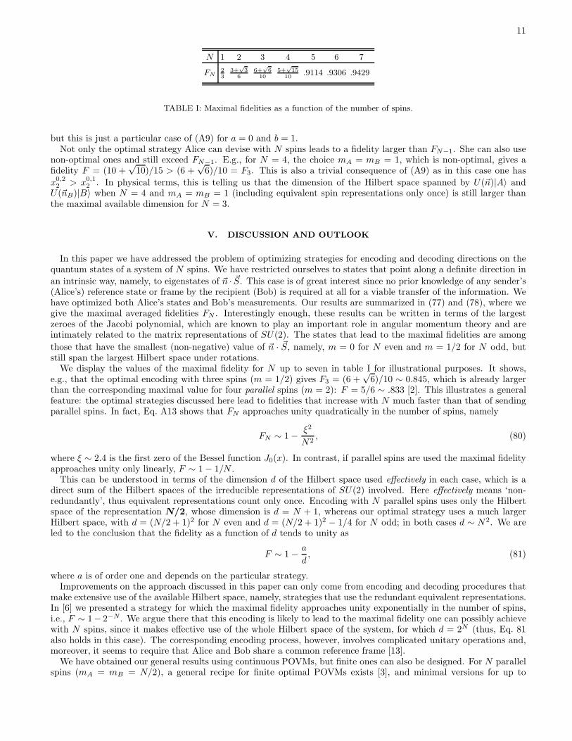
N 1 2 3 4 5 6 7

FN2

3

3+√

3

6

6+√

6

10

5+√

15

10.9114 .9306 .9429

TABLE I: Maximal fidelities as a function of the number of spins.

but this is just a particular case of (A9) for a = 0 and b = 1.Not only the optimal strategy Alice can devise with N spins leads to a fidelity larger than FN−1. She can also use

non-optimal ones and still exceed FN−1. E.g., for N = 4, the choice mA = mB = 1, which is non-optimal, gives afidelity F = (10 +

√10)/15 > (6 +

√6)/10 = F3. This is also a trivial consequence of (A9) as in this case one has

x0,22 > x0,1

2 . In physical terms, this is telling us that the dimension of the Hilbert space spanned by U(~n)|A〉 andU(~nB)|B〉 when N = 4 and mA = mB = 1 (including equivalent spin representations only once) is still larger thanthe maximal available dimension for N = 3.

V. DISCUSSION AND OUTLOOK

In this paper we have addressed the problem of optimizing strategies for encoding and decoding directions on thequantum states of a system of N spins. We have restricted ourselves to states that point along a definite direction in

an intrinsic way, namely, to eigenstates of ~n · ~S. This case is of great interest since no prior knowledge of any sender’s(Alice’s) reference state or frame by the recipient (Bob) is required at all for a viable transfer of the information. Wehave optimized both Alice’s states and Bob’s measurements. Our results are summarized in (77) and (78), where wegive the maximal averaged fidelities FN . Interestingly enough, these results can be written in terms of the largestzeroes of the Jacobi polynomial, which are known to play an important role in angular momentum theory and areintimately related to the matrix representations of SU(2). The states that lead to the maximal fidelities are among

those that have the smallest (non-negative) value of ~n · ~S, namely, m = 0 for N even and m = 1/2 for N odd, butstill span the largest Hilbert space under rotations.

We display the values of the maximal fidelity for N up to seven in table I for illustrational purposes. It shows,e.g., that the optimal encoding with three spins (m = 1/2) gives F3 = (6 +

√6)/10 ∼ 0.845, which is already larger

than the corresponding maximal value for four parallel spins (m = 2): F = 5/6 ∼ .833 [2]. This illustrates a generalfeature: the optimal strategies discussed here lead to fidelities that increase with N much faster than that of sendingparallel spins. In fact, Eq. A13 shows that FN approaches unity quadratically in the number of spins, namely

FN ∼ 1 − ξ2

N2, (80)

where ξ ∼ 2.4 is the first zero of the Bessel function J0(x). In contrast, if parallel spins are used the maximal fidelityapproaches unity only linearly, F ∼ 1 − 1/N .

This can be understood in terms of the dimension d of the Hilbert space used effectively in each case, which is adirect sum of the Hilbert spaces of the irreducible representations of SU(2) involved. Here effectively means ‘non-redundantly’, thus equivalent representations count only once. Encoding with N parallel spins uses only the Hilbertspace of the representation N/2, whose dimension is d = N + 1, whereas our optimal strategy uses a much largerHilbert space, with d = (N/2 + 1)2 for N even and d = (N/2 + 1)2 − 1/4 for N odd; in both cases d ∼ N2. We areled to the conclusion that the fidelity as a function of d tends to unity as

F ∼ 1 − a

d, (81)

where a is of order one and depends on the particular strategy.Improvements on the approach discussed in this paper can only come from encoding and decoding procedures that

make extensive use of the available Hilbert space, namely, strategies that use the redundant equivalent representations.In [6] we presented a strategy for which the maximal fidelity approaches unity exponentially in the number of spins,i.e., F ∼ 1− 2−N . We argue there that this encoding is likely to lead to the maximal fidelity one can possibly achievewith N spins, since it makes effective use of the whole Hilbert space of the system, for which d = 2N (thus, Eq. 81also holds in this case). The corresponding encoding process, however, involves complicated unitary operations and,moreover, it seems to require that Alice and Bob share a common reference frame [13].

We have obtained our general results using continuous POVMs, but finite ones can also be designed. For N parallelspins (mA = mB = N/2), a general recipe for finite optimal POVMs exists [3], and minimal versions for up to

12

N = 7 can be found in [4]. The unit vectors ~nr associated to the outcomes of these POVMs are the vertices ofcertain polyhedra inscribed in the unit sphere. For N ≤ 7 we have explicitly verified that these very same polyhedracan be use to design finite optimal POVMs for any value of mA = mB ≤ N/2. Moreover, the minimal POVMsof [4] remain minimal for the states considered here. We have discussed this issue in detail for N = 2 in section II.For N = 3 the polyhedron corresponding to the minimal POVM is the octahedron [4]. One can easily verify thatOr = U(~nr)|B〉〈B|U †(~nr), where |B〉 is given in (39) with mB = 1/2, 3/2, fulfill the completeness condition (2). Wehence believe that the discretization of a continuous POVM is a geometrical problem, i.e., it seems to be independentof the states |B〉.

The optimal states, |A〉, can be easily computed from the matrix M in (50), as they are the eigenvectors corre-sponding to the maximal eigenvalue. Recall that for N = 2 one obtains the one-parameter family of states (21) whichincludes the product states | ↑↓〉, | ↓↑〉. For N > 2, product states of the type | ↑↓↑↑↓ · · ·〉 do not seem to be optimal.Consider, e.g., N = 4. The optimal eigenvector of M is

|A〉 =

√2

3|2, 0〉 + eiγ1

1√2|1, 0〉+ eiγ0

√

5

18|0, 0〉, (82)

which is clearly not a product state of the individual spins for any choice of the phases [14]. One could argue that thissolution is not entirely general because the Clebsch-Gordan series of (1/2)⊗4 contains the representation 1 three timesand 0 twice, whereas in (82) they appear only once. However, any optimal state has the same ‘effective’ components

Aj (see eqs. 75-76), which can be read off from (82):

A2 =

√2

3, A1 =

1√2, A0 =

√

5

18. (83)

Note now that any product state with m = 0 (two spins up and two spins down), e.g., | ↑↑↓↓〉, | ↑↓↓↑〉, has an ‘effective’

Clebsch-Gordan decomposition given by A2 = A1 = A0 = 1/√

3, which do not coincide with (83). Therefore, these

product states cannot be optimal. Nevertheless, they lead to a maximal fidelity F = (15 + 5√

2 + 2√

5)/30 ≈ 0.885,which is remarkably close to F4 ≈ 0.887. This is likely to be the case for arbitrary N . These issues are currentlyunder investigation.

Acknowledgments

We thank S. Popescu, A. Bramon, G. Vidal and W. Dur for stimulating discussions. Financial support fromCICYT contracts AEN98-0431, AEN99-0766, CIRIT contracts 1998SGR-00026, 1998SGR-00051, 1999SGR-00097and EC contract IST-1999-11053 is acknowledged.

APPENDIX A:

In this appendix we collect the mathematical properties of the Jacobi polynomials P a,bn (x) that we use in the text.

We are concerned only with integer values of a and b such that b ≥ a ≥ 0. Further properties can be found in [12]and [15].

For fixed a and b, P a,bn (x) is a set of orthogonal polynomials, where n labels the degree of each polynomial in the

set. A convenient definition can be stated in terms of their Rodrigues formula:

P a,bn (x) =

(−1)n

2nn!(1 − x)−a(1 + x)−b dn

dxn

[

(1 − x)n+a(1 + x)n+b]

. (A1)

From (A1) it follows the recursion relation:

xP a,bn (x) = αnP a,b

n+1(x) + βnP a,bn (x) + γnP a,b

n−1(x), (A2)

with

αn =2(n + 1)(n + a + b + 1)

(2n + a + b + 1)(2n + a + b + 2),

βn =b2 − a2

(2n + a + b)(2n + a + b + 2),

γn =2(n + a)(n + b)

(2n + a + b)(2n + a + b + 1). (A3)

13

It also follows the differentiation formula

d P a,bn (x)

dx=

n + a + b + 1

2P a+1,b+1

n−1 (x). (A4)

The normalization is chosen so that the coefficient An of the highest power of P a,bn (x) = Anxn + Bnxn−1 + · · · is

An =Γ(2n + a + b + 1)

2nn!Γ(n + a + b + 1). (A5)

The following two relations can also be obtained from the definition A1:

(2n + a + b)P a,b−1n (x) = (n + a + b)P a,b

n (x) + (n + a)P a,bn−1(x), (A6)

(n + b + a + 1)1 + x

2P a,b+1

n (x) = (n + 1)P a,b−1n+1 (x) + bP a,b

n (x). (A7)

Let us recall some basic facts about the zeros of orthogonal polynomials: i) any orthogonal polynomial, Pn, of ordern has n real simple zeros. For Jacobi polynomials these zeros lie in the interval (−1, 1); ii) the zeros of Pn and Pn+1

are interlaced; iii) for x greater than the largest zero, the polynomial is a monotonously increasing function (if thepolynomial is normalized as in Eq. A5, where An > 0). In particular, Pn(x) must be positive in this region .

Now we can prove the results needed in the text. As in there, we denote by xa,bn the largest zero of the polynomial

P a,bn (x). Let us start by showing that

xa+1,b+1n−1 < xa,b

n . (A8)

From property iii above it follows that the left hand side of (A4) is manifestly positive for x > xa,bn . Hence, so it is

the right hand side. We conclude that xa+1,b+1n−1 cannot belong to this region and (A8) follows

Next, we prove the inequality

xa,bn−1 < xa,b−1

n < xa,bn . (A9)

We evaluate (A6) at x = xa,bn and use properties ii (⇒ xa,b

n−1 < xa,bn ) and iii, which imply that P a,b

n−1(xa,bn ) > 0, to

obtain that P a,b−1n (xa,b

n ) > 0. We repeat the process for x = xa,bn−1 and conclude that P a,b−1

n (xa,bn−1) < 0. Hence

P a,b−1n has a zero in the interval (xa,b

n−1, xa,bn ). This is necessarily the largest zero xa,b−1

n since, according to (A6) and

properties ii and iii, P a,b−1n (x) > 0 for x > xa,b

n . Thus (A9) follows

The inequality

xa,b+1n < xa,b−1

n+1 (A10)

can be proven as follows. Evaluate (A7) at x = xa,b+1n so that the left hand side of this equation is zero. The second

inequality in (A9) and property iii imply that P a,bn (xa,b+1

n ) > 0. Hence the first term on the right hand side of (A7)

must be negative, i.e., P a,b−1n+1 (xa,b+1

n ) < 0, and (A10) follows immediately, since otherwise property iii would not hold

for P a,b−1n+1

For two given integers l, m consider now the following set of zeros

Clm = xm′′−m′,m′′+m′

l−m′′ : m ≤ m′ ≤ m′′ ≤ l. (A11)

We want to prove that

maxClm = x0,2m

l−m . (A12)

According to (A8), decreasing m′′ by one leads us to a larger zero. The maximum is then in the subset x0,2m′

l−m′ : m ≤m′ ≤ l. The inequality (A10) now implies (A12)

Finally, we give the large n (asymptotic) behavior of xa,bn [12]:

xa,bn = 1 − ξ2

a

2n2+ O(

1

n3), (A13)

14

where ξa is the first zero of the Bessel function Ja(x). For a = 0, which is relevant for our discussion in section V, wealso give the subleading term:

x0,bn = 1 − ξ2

0

2n2

(

1 − b + 1

n

)

+ O(1

n4), (A14)

where

ξ0 = ξ = 2.405. (A15)

[1] A. Peres and W. K. Wootters, Phys. Rev. Lett. 66, 1119 (1991).[2] S. Massar, Phys. Rev. Lett. 74, 1259 (1995) .[3] R. Derka, V. Buzek, A.K. Ekert, Phys. Rev. Lett. 80, 1571 (1998).[4] J.I. Latorre, P. Pascual, R. Tarrach, Phys. Rev. Lett. 81, 1351 (1998).[5] N. Gisin and S. Popescu, Phys. Rev. Lett. 83, 432 (1999).[6] E.Bagan et al., Phys. Rev. Lett. 85, 5230 (2000); quant-ph/0006075.[7] A. Peres and P. Scudo, quant-ph/00010085.[8] S. Massar, Phys. Rev. A62 (2000) 040101(R).[9] E.B. Davies, IEEE Trans. Inform. Theory IT-24, 596 (1978).

[10] A. S. Holevo, Probabilistic and Statistical Aspects of Quantum Theory, North Holland, Amsterdam, 1982.[11] W.K. Tung, Group Theory in Physics World Scientific Publishing, 1985; A.R. Edmonds, Angular Momentum in Quantum

Mechanics, Princeton University Press, 1960.[12] For standard definitions and conventions see, for instance: M. Abramowitz and I.A. Stegun, Handbook of Mathematical

Functions, Dover, New York 1970.[13] A. Peres, private communication.[14] If we consider this state as a bipartite system of two spin 1 subsystems, it is also entangled for any choice of the phases

γ1, γ0.[15] A.F. Nikiforov and V.B. Uvarov, Special Functions of Mathematical Physics, Birkhasuer, Basel, 1988.