Optimal Dithering Configuration Mitigating Rayleigh ... - arXiv

1

Optimal Dithering Configuration MitigatingRayleigh-Backscattering-Induced Distortion in

Radioastronomic Optical Fiber SystemsJacopo Nanni, Andrea Giovannini, Enrico Lenzi, Simone Rusticelli, Randall Wayth ˜Member, ˜IEEE,

Federico Perini, Jader Monari, Giovanni Tartarini ˜Member, ˜IEEE

Abstract—In the context of Radioastronomic applicationswhere the Analog Radio-over-Fiber technology is used for theantenna downlink, detrimental nonlinearity effects arise becauseof the interference between the forward signal generated by thelaser and the Rayleigh backscattered one which is re-forwardedby the laser itself toward the photodetector.

The adoption of the so called dithering technique, whichinvolves the direct modulation of the laser with a sinusoidaltone and takes advantage of the laser chirping phenomenon, hasbeen proved to reduce such Rayleigh Back Scattering - inducednonlinearities. The frequency and the amplitude of the ditheringtone should both be as low as possible, in order to avoid undesiredcollateral effects on the received spectrum as well as keep at lowlevels the global energy consumption.

Through a comprehensive analysis of dithered Radio over Fibersystems, it is demonstrated that a progressive reduction of thedithering tone frequency affects in a peculiar fashion both thechirping characteristics of the field emitted by the laser and thespectrum pattern of the received signal at the fiber end.

Accounting for the concurrent effects caused by such phe-nomena, optimal operating conditions are identified for the im-plementation of the dithering tone technique in radioastronomicsystems.

Index Terms—Nonlinearities; Rayleigh backscattering; Ra-dioastronomy, RoF, Laser feedback, Dithering.

I. INTRODUCTION

SYSTEMS which adopt the Radio-over Fiber (RoF) tech-nology in one of its most cost-efficient versions consist

essentially in a radiofrequency (RF) signal which performsthe direct intensity modulation (D-IM) of a laser source,propagates in a span of Standard Single Mode Fiber (SSMF)and is directly detected (DD) at the receiver end (D-IMDDRoF systems) [1]–[3].

When the described scheme is utilized within Radioas-tronomic scenarios, peculiar features have to be considered,

J. Nanni, A. Giovannini and G. Tartarini are with the Dipartimento di Ingeg-neria dell’Energia Elettrica e dell’Informazione “Guglielmo Marconi”, Univer-sita di Bologna, 40136 Bologna (BO), Italy (e-mail: [email protected];[email protected]; [email protected]).

S. Rusticelli is with 3PSystem s.r.l, via Riviera delBrenta 170, 30032 Fiessod’Artico (VE), Italy (e-mail:[email protected]).

F. Perini, J. Monari are with Institute of Radio Astronomy, National Institutefor Astrophysics, Via Fiorentina 3513, 40059 Medicina (BO), Italy (e-mail:[email protected];[email protected];[email protected]).

E. Lenzi is with RF Optics di Enrico Lenzi, Via Sopra Castello 21, 40061,Minerbio (BO), Italy (e-mail:[email protected]).

R. Wayth is with ICRAR/Curtin University, Bentley Western Australia,6102 (e-mail:[email protected]).

which distinguish these systems e.g. from those which applythe D-IMDD RoF technology to the mobile network.

One of them is related to the frequencies of the transmittedRF signals, which in the case of the mobile network (4G, 5Gsignals and beyond) can reach several tens of GHz, and do notfall below around 700MHz [2], [3], while within Radioastro-nomic application can also belong to intervals ranging fromfew tens to few hundreds MHz [4], [5].

In addition to this, while RoF systems for the mobilenetwork are typically designed assuming that at the opticaltransmitter’s side the RF powers of the signals range roughlyin an interval of ± few units of dBm, in the case of signalsreceived by radioastronomic antennas these powers can exhibitvalues of just -60dBm when they come from astronomicalsources, while they arrive to a maximum of around -20dBmwhen they consist in undesired Radio Frequency Interference(RFI) signals coming from satellites, radio and/or televisiontransmitters, etc. [6].

As a consequence of the low power levels of the signalswhich directly modulate the laser source, in many RoF D-IMDD systems utilized for radioastronomic applications itis relatively straightforward to reduce to negligible valuesthe nonlinearities which typically bring detriment to RoFsystems in the mobile networks. Indeed, the spurious frequen-cies caused by the nonlinearity of the laser Power-Current[7] curves typically in this case fall below the noise floor.Moreover, it is enough to operate in the vicinity of thesecond optical window (around the wavelength λ = 1310nm),to guarantee that, due to the low level of the RF powermodulating the laser, the creation of nonlinearities generatedby the combined effect of laser chirp and fiber chromaticdispersion is avoided [8].

It has however been shown that in this kind of systems aprimary cause of undesired nonlinear effects takes place whena generic RFI signal (with frequency and angular frequencygiven respectively by fRF and ωRF = 2πfRF ) is transmittedin the RoF System together with the signals coming fromsky sources, after that they have all been received by theRadioastronomic antenna [9]. Indeed, the portion of suchRFI signal which is reflected by Rayleigh Backscattering(RB) reaches the laser section, is partly reflected again andinteracts at the receiver end with the transmitted RFI signalitself, generating nonlinear frequency terms (e.g. at frequencies2fRF , 3fRF , ....). Although the RFI disturbance at frequencyfRF can be filtered out at the signal post-processing stage,

arX

iv:2

207.

0022

4v1

[as

tro-

ph.I

M]

1 J

ul 2

022

2

the same cannot be done for all generated spurious frequencyterms.

One countermeasure to the described problem could be rep-resented by the introduction of a further optical isolator at thefiber input section, which would be added to the one embeddedin the laser. However this solution would hardly meet thecost limitations (e.g. possibly 100USD or less for a singlefront-end receiver) imposed by the very high number of RoFdownlinks which should be realized within radioastronomicfacilities operating at frequencies of tens/hundreds of MHz[4], [10]–[14].

In a previous work, an appropriate cost-effective solutionhas been demonstrated, consisting in the introduction of adithering tone as a further modulation current for the opticaltransmitter, which pushes the level of the nonlinear termsbelow the noise floor [15], [16].

This solution had actually already been proposed in thepast, within telecommunication scenarios, with the aim toreduce noise effects in optical fiber systems [17], [18], andits application finalized to the reduction of the spurious termsconstitutes an additional newly-evidenced advantage offeredby this technique.

In the application of the mentioned dithering tone techniqueit would however be desirable that both the frequency fd(or angular frequency ωd = 2πfd) and the amplitude Idof the current tone exhibit the lowest possible values. Thefirst requirement is related to the fact that the distance fromfRF of the possibly generated spurious frequency terms,fRF ± fd, fRF ± 2fd, ... should be lower than the resolutionbandwidth of the reception filter, so that they can be removedfrom the received signal together with the RFI term at fre-quency fRF . The second requirement comes instead from thenecessity to keep at low levels the energy consumption of thetone generator.

To assist the designer in identifying the appropriate solutionto the problem, a theoretical model of the laser behaviorunder current modulation in presence of optical feedbackby RB is necessary. However, the models developed so fardescribing the effects produced by optical feedback underlaser current modulation, are not referred to RB, since theyconsider only the reflection coming from a single externalcavity [19]–[21], typically put on the back-facet of the laser.At the same time, the effects produced by RB feedback havebeen considered only with reference to the linewidth reduction[22] and optical frequency shift and hopping [23], [24], in allcases for continuous-wave operation, without considering thepresence of a modulating current.

In the present paper, a rigorous mathematical model basedon the laser Rate Equations is developed to describe the effectsof the feedback due to Rayleigh Backscattering on an opticalfield modulated by an RF signal. The model, which will beshown to be in agreement with experimental measurements,is utilized to describe the effects of the introduction of thedithering tone and to identify the optimal working point whichallows keep both Id and ωd as low as possible.

The paper is organized as follows: Section II provides adescription of the model developed to study the impact ofRB on the characteristics of the field emitted by a directly

Fig. 1: Scheme of the structure considered.

modulated laser. Section III describes the experimental results,which confirm the correctness of the theoretical model adoptedand allow to identify the optimal operating conditions forthe implementation of the dithering tone technique. Finally,conclusions will be drawn.

II. THEORETICAL MODEL

The theoretical model presented in this work is based onthe physical structure shown in Figure 1, composed by alaser-based optical transmitter whose emitted field is coupledthrough a focusing lens and an isolator to an optical fiberand reaches finally an optical receiver based on a PIN pho-todetector. The laser cavity, exhibits a length Lcav and powerreflectivities at the facets Rl,1 and Rl,2, respectively. Theinjection current Iinj(t) can be written in complex notation asIinj(t) = Ibias +

∑i Iie

jωit, where Ibias represents the biascurrent, and Ii represents the amplitude of the generic i− thsinusoidal RF tone which directly modulates the laser, withangular frequency ωi and frequency fi = ωi/(2π). For formalsimplicity and without loss of generality, in the following onlytwo modulating tones will be considered, namely a term withamplitude IRF and angular frequency ωRF = 2πfRF , andthe so called dithering tone with amplitude Id and angularfrequency ωd = 2πfd, resulting in:

Iinj(t) = Ibias + Idejωdt + IRF e

jωRF t (1)

For this reason, instead of∑i=d,RF . . . , the simplified

notation∑i . . . will be adopted throughout the paper.

In principle, the electrical field emitted by the laser sourceand propagating into the fiber should be represented in vectorform, to account for the evolution of its state of polarization(SOP). However, the phenomenon of Rayleigh backscattering,which takes place within the fiber in correspondence to thereflection sections zk, k = 1, . . . ,K (see again Figure 1) canbe regarded as substantially isotropic, while the change of theSOP of the field between zk and an adjacent section can bedescribed by an appropriate Jones matrix, which is unitary.Consequently, it can be shown that for a given initial SOPand in absence of Polarization Dependent Losses (PDL), theelectrical field exhibits at the fiber end section a correspondingfinal SOP on which the quantities which are of interest in thepresent work (e.g. powers received at different frequencies) donot depend [25], [26].

3

In presence of Polarization Dependent Losses (PDL), thequantities which are of interest in the present work can insteadexhibit variations depending on the final SOP of the electricfield. This could be appreciated for example in presence ofchanges of environmental quantities (e.g. temperature). Indeed,while it can be reasonably assumed that the devices locatedwithin the transmitter (single-mode laser, lens, isolator) stilldetermine a stable SOP for the emitted field, the opticalfiber can undergo local birefringence perturbations which canchange in real time the SOP of the field impinging thedetecting area of the PIN. In presence of PDL of this lastdevice, the received powers would then exhibit a polarization-dependent fluctuating behavior. However the relative variationsof the measured quantities can be typically considered as low(e.g.few tenths of dB or less), and, at the same time, onfiber connections of the order of few km length, like the onesconsidered in this work, they can be appreciated on time scales(e.g. tens of seconds or more) which are much longer than theones of the phenomena investigated [6].

For all these reasons, in the rest of the paper the electricalfield will be described as a scalar quantity without losing thegenerality of the results that will be obtained.

A. Re-transmitted and re-injected portions of the RayleighBackscattered field

By virtue of the considerations developed above, the elec-trical field generated inside the laser can be expressed as

E(t) = |E(t)|ej[ω0t+θ(t)]ejφ(t) (2)

where |E(t)| is its module, ω0 the optical angular frequencythat the field would exhibit in absence of modulating tones andin absence of RB as well, θ(t) is the time-varying phase dueto their presence, while φ(t) represents the laser phase noisecontribution. The expressions of |E(t)| and θ(t) are given by:

|E(t)| = E0

√1 + ζRB +

∑i

micos(ωit) (3)

θ(t) = ∆ωt +∑i

|Mi|cos(ωit+ ∠Mi) (4)

In (3) E0 =√η(Ibias − Ith) is the electrical field ampli-

tude, with Ith threshold current and η power-current slopeefficiency of the laser, ζRB represents a small increment tothe unit number under square root, which derives from thepresence of RB and will be further described in the nextsubsection, while mi = Ii/(Ibias− Ith) represents the opticalmodulation index at the considered frequency.

In (4) ∆ω represents a variation of the angular frequencydue to RB and to direct modulation, whose presence deter-mines the total optical angular frequency of the emitted fieldto be ωopt = ω0+∆ω. Moreover, the quantities |Mi| and ∠Mi

are respectively module and phase of the phase modulationindex due to the chirp effect at ωi [27].

In (2) the quantity ejφ(t) is a random function whosePower Spectral Density, determined as Fourier Transform ofits autocorrelation function, is given by:

Fξ⟨ejφ(t)−φ(t−ξ)

⟩= Fξ

e−|ξ|∆Ω

=

2∆Ω

∆2Ω + ω2

(5)

where Fξ· · · , 〈· · · 〉 indicate respectively the operations ofFourier Transformation with respect to the variable ξ, and timeaveraging. The quantity ∆Ω = 1/τcoh is the coherence angularfrequency band of the laser source, reciprocal of its coherencetime τcoh [28].

Still referring to Fig. 1, the field given by (2) exits thelaser right-hand-side facet, is focused by a coupling lens intoan isolator, and is subsequently injected at the input section(z = 0) of the optical fiber of length L, propagating with agroup velocity vg . Putting τ = z/vg , at the generic sectionz ∈ [0, L] of the fiber the resulting electric field can then bewritten as:

ETX(t, z) =√

1−Rl,2 ·√ηc · E(t− τ)e−αvgτ (6)

where ηc is the power coupling coefficient between the laserand the optical fiber given by the coupling lens, while α is theattenuation constant of the fundamental mode of the opticalfiber.

As above mentioned, as ETX propagates along the fiber,the phenomenon of Rayleigh backscattering takes place. Theinhomogeneity of the longitudinal profile of the refractiveindex of the optical fiber determines indeed the presence ofmany reflection points at the coordinates zk, k = 1, . . . ,K,each one of which generates a back reflected electrical field.At the output facet of the laser cavity a Rayleigh Backscatteredfield is then present, given by:

ERB(t) =

√1−Rl,2 · ηc√

αiso

K∑k=1

ρkE(t− 2τk)e−αvg2τk (7)

where αiso is the isolator power attenuation in the backwarddirection, while τk = zk/vg . Then, ρk = |ρk|ej∠ρk is thecomplex reflection coefficient at the k− th section due to RB.Note that the weak-feedback approximation, i.e. |ρk| << 1,is taken, meaning that possible multiple reflections within asingle fiber section are not considered.

The different ρk’s are assumed to be complex randomvariables, with zero mean value and Gaussian distribution.The variance of both their real and imaginary parts is σ2

ρ =12αsSdzk, where S is the so-called backscattering factor orrecapture factor, which depends on the characteristics of thefiber considered and exhibits typical values of the order of10−3 in case of the standard G.652 fiber, αs is the Rayleighattenuation coefficient, which for the considered wavelengthscan be assumed to coincide with α, and dzk = zk − zk−1 isthe length of the interval considered [29]. The ρk’s are alsoassumed to be delta-correlated, namely:

E[ρkρ∗h] = αsS dzkδkh (8)

4

where E[·] represents the expected value operator, while δkhis the delta Kronecker function [25].

Still referring to Fig. 1, a portion of the field reported in(7), given by ERB1(t) =

√1−Rl,2ERB(t), is re-injected

into the laser cavity. As will be shown in Subsection II-B,this fact has significant consequences on the phase modulationindex due to the chirp effect Md at ωd, which also influencesthe identification of the optimal frequency and amplitudecharacteristics of the dithering tone itself.

Another portion of this field, given by ERB2(t, z) =√Rl,2ERB(t, z) is instead reflected by the laser facet. As will

be shown in Subsection II-C, this reflected field adds to theone given by (6) in input to the optical fiber, contributing tothe final form of the power spectral density of the photocurrentdetected at the receiving end of the system. The knowledgeof the behavior of this quantity allows to put into evidenceparticular physical aspects which also contribute to determinethe optimal frequency and amplitude characteristics of thedithering tone to be utilized.

B. Re-injected portion of the RB field and effect on the Chirpterm

The Rate Equations, expressed below in the so calledSemi Classical form [7] [30] [31], describe the behaviors ofS(t) = |E(t)|2, θ(t) and N(t), which represent respectivelythe number of photons in the laser cavity, the previouslyintroduced time varying phase θ(t) and the carrier densityN(t), expressed in

[1m3

]:

dS(t)

dt=

(G(N,S)− 1

τp

)S(t) + ΓS(t) (9)

dθ(t)

dt=αH2GN (N(t)−Nth)− Γθ(t) (10)

dN(t)

dt=Iinj(t)

eV− N(t)

τs− G(N,S)

VS(t) (11)

At the second side of ((9)) the quantity G(N,S) is the lasercavity gain which depends both from N , and S through therelation:

G(N,S) =g0

1 + εS(N−Ntr) ' g0 ·(1−εS)(N−Ntr) (12)

where the transparency level Ntr is the density of carriersin the cavity for which G(N,S) = 0, ε << 1/S is the gaincompression factor and g0 represents the nominal gain-slope inabsence of compression, multiplied by the volume of the lasercavity [30]. The quantity τp represents the average photon’slifetime, or inverse of the cavity losses.

The term ΓS(t) at the right-hand-side of (9), which repre-sents the RB contribution to dS(t)/dt, is given by:

ΓS(t) = 2

K∑k=1

|Ck|√S(t)S(t− 2τk) ·

· cos[ω0 · 2τk + θ(t)− θ(t− 2τk)− ∠ρk] (13)

and will be derived in Appendix A. Within (13), Ck is thek-th compound-cavity coefficient [19] defined as follows:

Ck =(1−Rl,2)ηc√

αisoρke−αvg2τk

1

2τcav

1√Rl,2

(14)

where τcav = 2 ·ncavLcav/c is the round-trip time of the lasercavity with refractive index ncav .

By solving the laser rate equations in the reference steadystate case where both external RF modulation and RB feed-back are absent, it results that the carrier density is equal to theamount Nth which balances the cavity losses, and it resultsalso that number of photons is S0 =

τpe (Ibias − Ith) with

Ith = NtheVτs

, where the relationship τp = 1/G(Nth, S0) hasbeen exploited.

At the second side of (10) αH is the linewidth enhancementfactor of the laser source [30] while it is GN = ∂G

∂N

∣∣S0

=

g0(1− εS0).Similarly to (9), the last term at the right-hand-side of (10)

represents the RB contribution to dθ(t)/dt:

Γθ =

K∑k=1

|Ck|

√S(t− 2τk)

S(t)·

sin[ω0 · 2τk + θ(t)− θ(t− 2τk)− ∠ρk] (15)

and will also be derived in Appendix A.Finally, at the second side of (11) the quantities e, V , τs

represent respectively the electron charge, the volume of theactive region and the carrier-lifetime.

Assuming that partial RB field re-injection and RF modu-lation of the injection current determine only a perturbativeeffect on the laser emission characteristics, the behavior ofG(N,S) can be represented by its expansion to the first order:

G(N,S) ' G(Nth, S0) +GN (N −Nth) +GS(S−S0) (16)

where GS = ∂G∂S

∣∣Nth

= −g0ε(Nth −Ntr).Within the hypothesis taken, in presence of an injection

current Iinj(t) given by the second side of (1) S(t), θ(t) andN(t) exhibit expressions given by:

S(t) = S0 + ∆S +∑i

Siejωit (17)

θ(t) = ∆ωt+∑i

Miejωit (18)

N(t) = Nth + ∆N +∑i

Niejωit (19)

where (18) is (4) re-written in complex notation and where(∆S,∆ω,∆N), and (Si,Mi, Ni)∀i, are the unknowns which,within the perturbative regime taken, respect the conditions:

∆S, |Si|∀i << S0 (20)∆ω, |ωiMi|∀i << ω0 (21)∆N, |Ni|∀i << Nth (22)

In line with (20), (21), (22), it will be assumed that theperturbation caused the generic i − th modulating tone canbe determined separately from the one due to the other,namely that the expression of the triplet (Si, Mi, Ni) can be

5

TABLE I: Typical Orders of Magnitude of Rate EquationsParameters.

Symbol Physical meaning Order of Magnitudeg0 Gain slope ∼ 10−12 m3/secNtr Carriers Transparency Level ∼ 1. · 1024 m−3

Nth Carriers Threshold Level ∼ 2. · 1024 m−3

ε Gain compression factor ∼ 10−8

τp Photon Lifetime ∼ 10−12secτs Carrier Lifetime ∼ 10−9sec

Rl,1, Rl,2 Laser mirrors reflectivities ∼ 0.3, . . . , 0.5Lcav Laser cavity length ∼ few 100µmV Volume of Laser active region ∼ 10−16m3

ncav Laser cavity refractive index ∼ 3.5, . . . , 5αH Linewidth enhancement factor ∼ 3, . . . , 6

Number of photons in steady stateS0 (assuming for Ibias − Ith ∼ 105

a value of few tens mA)GN ∂G/∂N in steady state ∼ 10−12 m3

GS ∂G/∂S in steady state ∼ 104

determined just considering Iinj(t) = Ibias + Iiejωit (i = d

or i = RF ).Inserting the relations (17), (18), (19) with the summations

composed by one element into (9), (10), (11), and consideringthe terms at DC and at ωi of the Jacobi-Anger expansions of(13) and (15) (detailed in Appendix B), it is possible to obtaintwo systems of three equations. The first one, which is omittedfor brevity, represents the steady-state terms and allows todetermine ∆S,∆ω,∆N , while the second one represents themodulating terms with angular frequency ωi, which allow todetermine Si,Mi, Ni.

The latter of the two systems assumes the following form:

A ·

SiMi

Ni

=

00IieV

(23)

where the matrix A is given by:

A = (24)jωi −GSS0 +2S0γS,i −GNS0

0 jωi + γθ,i −αH

2 GN

1τpV

+ GSS0

V 0 jωi + 1τs

+ GNS0

V

and where the elements γS,i and γθ,i, located in positions

(1, 2) and (2, 2), are derived from ΓS and Γθ, as shown inAppendix B.

As will be evidenced in the next Subsection, the highervalues exhibited by the module |Md| of the phase modulationindex due to the chirp effect at ωd, the more effective thedithering technique results in reducing to negligible levelsthe undesired RB-related nonlinearities. For this reason, thebehavior of Mi, which is obtained by solving (24), will beanalyzed in the following.

In doing so, some simplifications can be taken, whichallow to put this quantity in a more readable form. Indeed,considering modulating frequencies fi which can range fromKHz to hundreds MHz, and assuming for Ibias a value suchthat Ibias − Ith ∼ few tens of mA, taking into account the

typical orders of magnitude of Rate Equations parametersreported in Table I, the determinant of A can be reduced to:

det[A]' GNS0

τpV[jωi + γRB,i] (25)

where it has been put:

γRB,i = γS,i − αHγθ,i '√

1 + α2H ·

K∑k=1

|Ck| · (26)

·2J1(Xi,k)

Xi,k

(1− e−jωi2τk

)cos(ψk − tan−1 αH

)with:

Xi,k = 2|Mi|sin(ωiτk + ∠Mi) (27)ψk = ωopt2τk − ∠ρk (28)

The resulting expected value of |Mi| is then given by theexpression:

|Mi| = E

[τpeαH

2 GS Ii√ω2i + |γRB,i|2

](29)

in which the statistical expectation can be straightforwardlyapplied through (8) and utilizing the properties of the ρk’sspecified in Section II-A. It can be at first noted that the valueof |Mi| are proportional to the amplitude of the modulatingcurrent Ii. Secondly, regarding the dependence of the fre-quency fi (or angular frequency ωi) of the modulating current,it can be first observed that in case the RB effects were absent,the value of |Mi| would result inversely proportional to ωi.

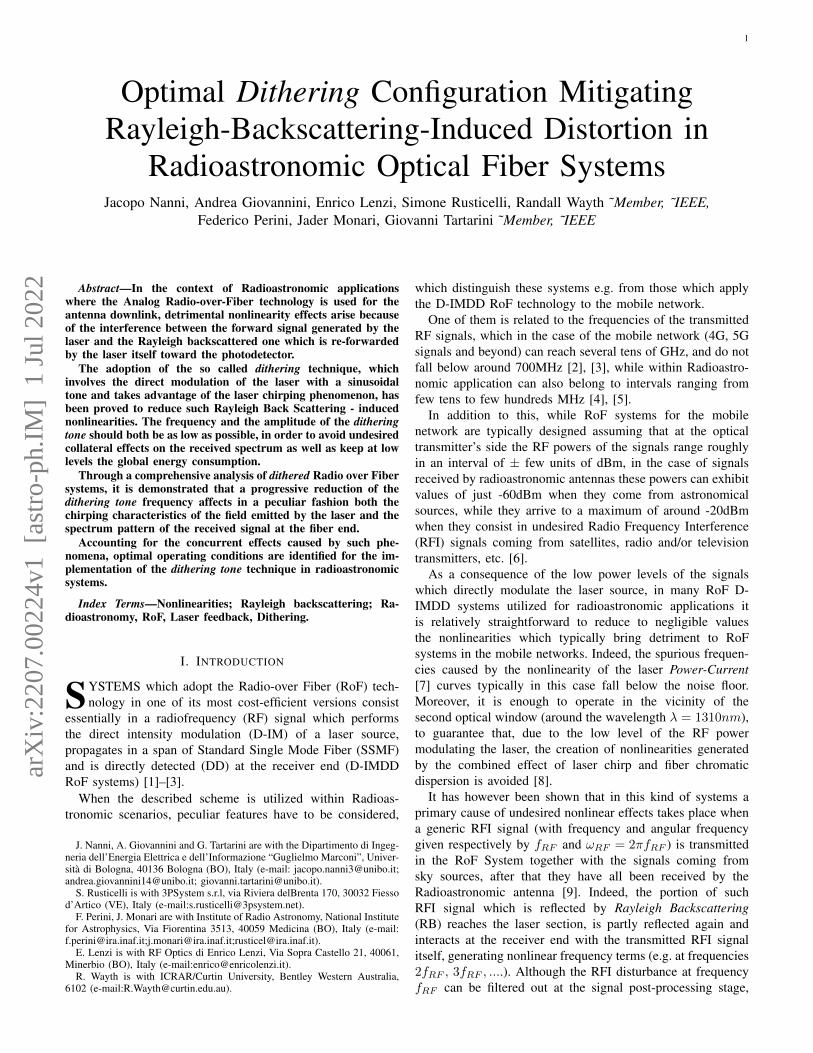
In the considered case, the dependence of |Mi| on ωi doesnot instead follow such simple pattern. Solving (29) iteratively(since |Mi| is contained in γRB,i) it is indeed possible toobtain the curves reported in Fig.2, which have been modelledin accordance with the orders of magnitude of the parametersreported in Table I and Table II.

At the right hand side of the figure it can be noted that forfrequencies greater than few hundred MHz it can effectivelybe assumed for all the reported curves |Mi| ' Kf,iIi

fiwhere

Kf,i = 12π

τpeαH

2 GS , is the so called adiabatic chirp factor,expressed in [Hz/A]. Indeed, a constant value |Mi| = 10n rad(n = 1, . . . , 6 in the figure) corresponds to the linear rela-tionship Ii = 10n rad

Kf,ifi. This is the behavior of |Mi| when

i = RF is considered, since the undesired RFI signals whichaffect radioastronomic plants operating in the lower bandwidthof the radioastronomic spectrum exhibit frequencies of tens tohundreds of MHz [16].

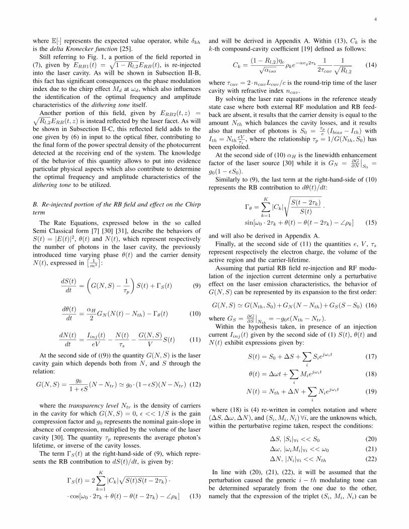
When instead the dithering tone is considered (i = d), it ishowever convenient to give lower values to fd. For example,a given constant value |Md| = 103 rad would be obtainedwith Id ' 10 mA if fd ' 2 MHz were chosen, but can beobtained with Id ' 0.1 mA if fd ' 20 kHz. Note that givinglow values to fd fulfills also the requirement to keep the termsfRF ± fd, fRF ± 2fd, ... within the resolution bandwidth ofthe reception filter, as mentioned in the Introduction.

6

Fig. 2: Values of the modulating current amplitude Ii which,for a given modulating frequency fi determine assigned valuesof the module of the phase modulation index due to theadiabatic chirp |Mi|. Continuous lines: realistic cases wherethe effect of RB is taken into account. Dashed lines: theoreticalvalues of Ii in case no RB field re-injection were present. Notethat the subscripts can be assumed as i = RF or i = d.

Still considering as example the curve referred to the value|Md| = 103 rad, it can however also be noted that for frequen-cies lower than few kHz the value of Id to be utilized becomespractically independent from fd. This happens because, as canbe shown with a detailed analysis of its composing terms,|γRB,d| is weakly dependent on the frequency. Going thereforefrom right to left in the horizontal axis of Fig.2, sooner orlater ωd reaches values lower than |γRB,d| so that the secondside of (29) becomes almost independent from fd. The sameconsiderations apply for the other curves |Md| = constant,with the difference that the values of the frequencies at whichthe lines become independent from fd decrease for increasingvalues of |Md| (or increase for decreasing values of |Md|).This behavior can be intuitively explained, since an increaseof |Md| determines an increase of Xd,k (see (27)) whichin turn brings to a reduction of the terms 2J1(Xd,k)

Xd,kof the

sum present in (26), i.e. a decrease of the “cutoff angularfrequency” |γRB,d|.

Still in Fig. 2 the behavior of |Md| in case of absence ofRB is also reported, which puts into evidence the describedeffect of the RB field re-injection, namely the impossibility at agiven low frequency to obtain high values of |Md| for ditheringcurrent amplitudes lower than a minimum “threshold” value.

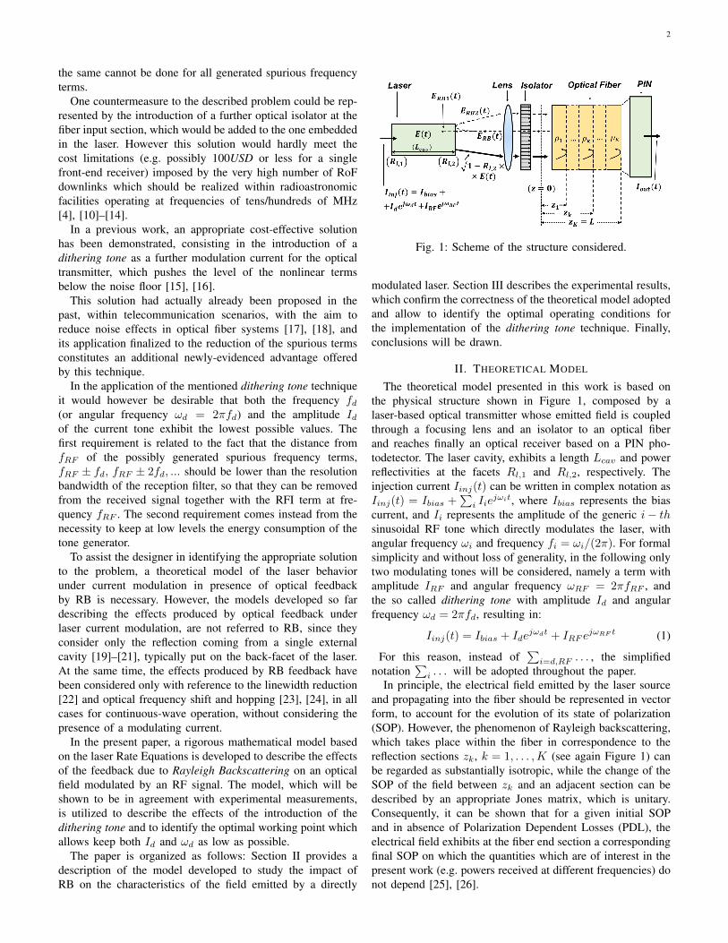
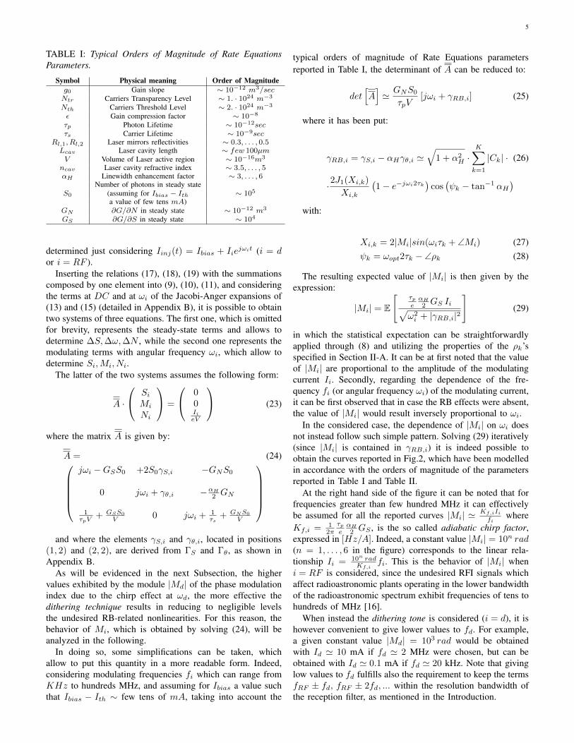
Note however that minimal increases of Id from this“threshold” value lead to very high variations of |Md|. This canbe appreciated in Fig. 3, which focalizes the same quantitiesrepresented in Fig. 2 in limited ranges of fd and Id.

Given the mentioned requirements for an effective applica-tion of the dithering tone technique (high |Md|, Id, fd as lowas possible), the practical indication is then to utilize a valueof Id around such ”threshold” value, while keeping fd as lowas possible. A further physical phenomenon will be howeverhighlighted in the next Section, which prevents the choice ofarbitrarily low values for fd.

Fig. 3: Values of |Mi| which are reached in the interval fi ∈[1, 10] kHz in the vicinity of the values of Ii where the curvesof Fig.2 appear to exhibit an almost horizontal behavior. Notethat the subscripts can be assumed as i = RF or i = d.

C. Power Spectral Density at the Receiving End and effectsof the Dithering Tone characteristics

As mentioned at the end of Section II.A, at the final endz = L of the fiber connection, the field received by the PINphotodetector is given by the sum ETX(t, L) + ERB2(t, L),with the first addend given by (6) with τ = τL = L/vg , andthe second one given by:

ERB2(t, L) =

√Rl,2(1−Rl,2) · η3/2

c√αiso

×

×K∑k=1

ρkE(t− 2τk − τL)e−αvg(2τk+τL) (30)

The current generated by the photo-detector can then becomputed as:

iout(t) = R|ETX(t, L) + ERB2(t, L)|2

= R · |ETX(t, L)|2 +R · |ERB(t, L)|2 +

+R · 2<eETX(t, L) · E∗RB(t, L) (31)

where R is the Responsivity of the detector.At the right-end-side of Equation (31), the first addend

would coincide with the total detected current if the RB effectwere absent. Moreover, the term |ERB(t, L)|2 is much smallerwith respect to the others therefore the second added will beneglected in the following.

In order to analyze the RB-induced spurious terms in thecurrent power spectrum, only the last addend at the righthand side of (31) has then to be considered, which will benamed as ioutTX,RB

. From Equations (6) (with τ = τL) and(30), exploiting the prostaferesis formula cos(u) − cos(v) =−2 sin

(u−v

2

)sin(u+v

2

)with u = ωi(t − τL) + ∠Mi and

7

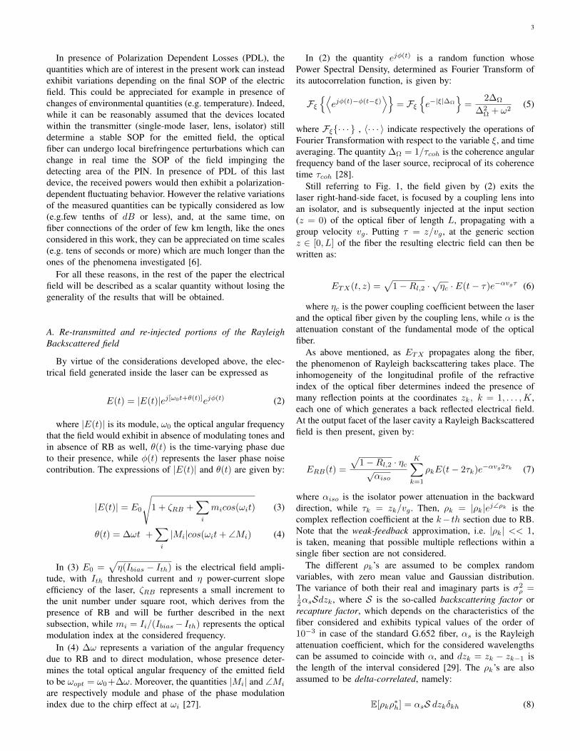
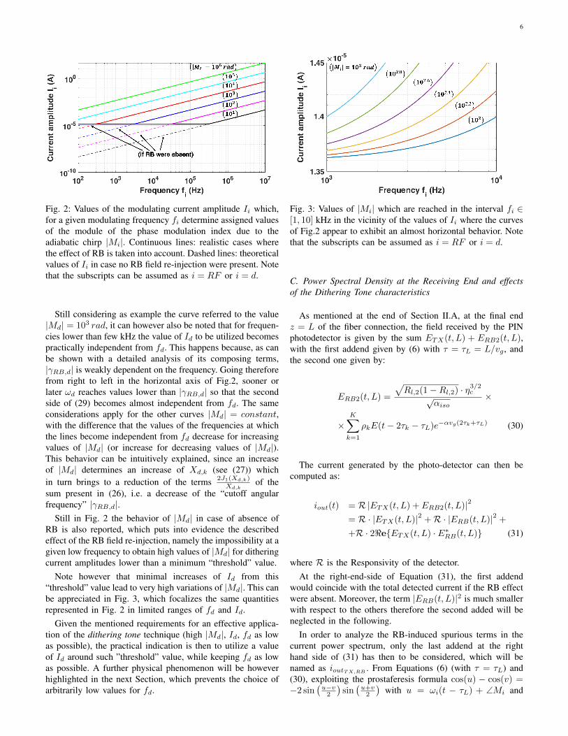
Fig. 4: Qualitative representation of the behavior ofPSDTX,RB(ω) in the vicinity of ω = 2ωRF , represented by(33) with nRF = 2, for the k − th elementary RB reflection,when ωd is sufficiently greater than ∆Ω. In this case the powerof the second-harmonic distortion term P2ωRF

practicallyconsists in the only element corresponding to nd = 0.

v = ωi(t− τL − 2τk) + ∠Mi, its expression results to be:

ioutTX,RB(t) ' R

√Rl,2αiso

(1−Rl,2)η2c |E(t− τL)|× (32)

× 2<e

kmax∑k=1

ρ∗k|E(t− 2τk − τL)|e−αvg2τk+jωopt2τk×

× ej−∑

iXi,ksin[ωi(t−τk−τL)+∠Mi]+φ(t−τL)−φ(t−2τk−τL)

where Xi,k has been defined in (27).In line with the perturbative approach adopted, in (32) both

field modules can be assumed to be equal to E0. Collecting allthe constants in a unique term Υ = R

√Rl,2

αiso(1−Rl,2)η2

cE20 ,

and exploiting the Jacobi-Anger expansion e−ju sin(v) =∑∞n=−∞ Jn(u)e−jnv , where u = Xi,k and v = ωi(t − τL −

τk) + ∠Mi, taking advantage of (5) and (8), after a lengthybut straightforward derivation, the expected value of the powerspectral density PSDTX,RB of ioutTX,RB

(t) assumes thefollowing expression:

PSDTX,RB(ω) =

= Fξ

E[⟨ioutTX,RB

(t)i∗outTX,RB(t− ξ)

⟩]'

' Υ2kmax∑k=1

σ2ρke−4αvgτk

+∞∑nd,nRF =

=−∞

J2nd

(Xd,k)J2nRF

(XRF,k)×

× 2∆Ω

∆2Ω + [ω − (ndωd + nRFωRF )]2

(33)

Focusing for example in the vicinity of ω = 2ωRF ,i.e. considering nRF = 2 in (33), and referring to thegeneric contribution related to the k − th elementary RBreflection, the function PSDTX,RB(ω), as can be appreciatedin Fig. 4, consists in the superposition of lorentzian func-tions centered in 2ωRF , 2ωRF ± ωd, 2ωRF ± 2ωd, . . . withamplitudes proportional respectively to J2

2 (XRF,k)J20 (Xd,k),

J22 (XRF,k)J2

±1(Xd,k), J22 (XRF,k)J2

±2(Xd,k), ....The power of the undesired second-harmonic distortion term

P2ωRFwithin an elementary bandwidth δΩ centered in 2ωRF

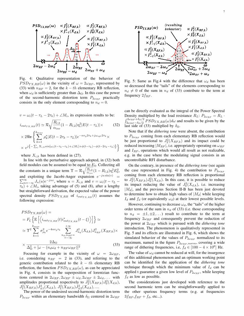
Fig. 5: Same as Fig.4 with the difference that ωd has beenso decreased that the “tails” of the elements corresponding tond 6= 0 of the sum in nd of (33) contribute to the term atfrequency 2fRF .

can be directly evaluated as the integral of the Power SpectralDensity multiplied by the load resistance RL: P2ωRF

= RL ·∫ 2ωRF +δΩ/2

2ωRF−δΩ/2 PSDTX,RB(ω)dω and results to be given by thelast side of (33) multiplied by δΩ.

Note that if the dithering tone were absent, the contributionto P2ωRF

coming from each elementary RB reflection wouldbe just proportional to J2

2 (XRF,k) and its impact could bereduced increasing |MRF |, i.e. appropriately operating on ωRFand IRF , operations which would all result as not realizable,e.g. in the case where the modulating signal consists in anuncontrollable RFI disturbance.

On the contrary, in presence of the dithering tone (see againthe case represented in Fig. 4) the contribution to P2ωRF

coming from each elementary RB reflection is proportionalto J2

2 (XRF,k)J20 (Xd,k). In this case, it is possible to reduce

its impact reducing the value of J20 (Xd,k), i.e. increasing

|Md|, and the previous Section II-B has been just devotedto determine how to obtain high values of |Md| while keepingId and fd (or equivalently ωd) at their lowest possible levels.

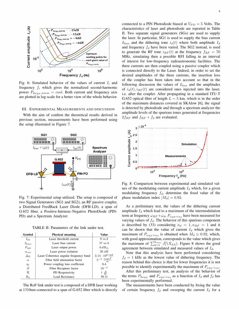
However, continuing to decrease ωd, the “tails” of the higherorder terms of the sum in nd of (33) (i.e. those correspondingto nd = ±1,±2, . . . ) result to contribute to the term atfrequency 2ωRF and consequently prevent the reduction ofthe power at 2ωRF which is pursued with the dithering toneintroduction. The phenomenon is qualitatively represented inFig. 5 and its effects are illustrated in Fig. 6, which shows thesimulated behavior of the values of P2ωRF

normalized to itsmaximum, named in the figure P2ωRF ,norm, covering a widerange of dithering frequencies, i.e, fd ∈ [100− 4× 106] Hz.

The value of ωd cannot be reduced at will, for the insurgenceof this additional phenomenon and an optimum working pointcan be identified for the application of the dithering tonetechnique through which the minimum value of Id can beapplied t guarantee a given low level of P2ωRF

, while keepingfd as low as possible.

The considerations just developed with reference to thesecond harmonic term can be straightforwardly applied tothe other spurious frequency terms (e.g. at frequencies3fRF ,fRF + fd, etc...).

8

Fig. 6: Simulated behavior of the values of current Ii andfrequency fi which gives the normalized second-harmonicpower P2ωRF ,norm = cost. Both current and frequency axisare plotted in log-scale for a better view of the whole behavior.

III. EXPERIMENTAL MEASUREMENTS AND DISCUSSION

With the aim of confirm the theoretical results derived inprevious section, measurements have been performed usingthe setup illustrated in Figure 7.

Fig. 7: Experimental setup utilized. The setup is composed oftwo Signal Generators (SG1 and SG2), an RF passive coupler,a Distributed FeedBack Laser Diode (DFB-LD), a span ofG.652 fiber, a Positive-Intrinsic-Negative PhotoDiode (PIN-PD) and a Spectrum Analyzer.

TABLE II: Parameters of the link under test.

Symbol Physical meaning ValueIth Laser threshold current 9 mAIbias Laser bias current 37 mAPopt Laser output power 6 dBm

αiso Laser power isolation 20 dB∆Ω Laser Coherence angular frequency band 3.14 · 106 rad

s

α Fiber field attenuation factor 5−5 neperm

ηc Power coupling lens coefficient 0.4S Fiber Recapture factor 10−3

R PD Responsivity 1 AW

RL Load Resistance 50 Ω

The RoF link under test is composed of a DFB laser workingat 1310nm connected to a span of G.652 fiber which is directly

connected to a PIN Photodiode biased at VPD = 5 Volts. Thecharacteristics of laser and photodiode are reported in TableII. Two separate signal generators (SGs) are used to supplythe laser. In particular, SG1 is used to supply the bias currentIbias and the dithering tone id(t) where both amplitude Idand frequency fd have been varied. The SG2 instead, is usedto generate the RF tone iRF (t) at the frequency fRF = 70MHz, simulating then a possible RFI falling in an intervalof interest for low-frequency radioastronomic facilities. Thethree currents are then coupled using a passive coupler whichis connected directly to the Laser. Indeed, in order to set thedesired amplitudes of the three currents, the insertion lossof the coupler has been taken into account so that in thefollowing discussion the values of Ibias and the amplitudesof id(t), iRF (t) are considered ones injected into the laser,i.e. after the coupler. After propagating in a standard ITU-TG.652 optical fiber of length L = 5 km, which is in the orderof the maximum distances covered in SKAlow [6], the signalis detected by photodiode and through a spectrum analyzer theamplitude levels of the spurious tones generated at frequencies2fRF and fRF + fd are evaluated.

104 106

Frequency fd (Hz)

0

0.5

1

1.5

2

2.5

3C

urr

ent

amp

litu

de

I d (

A)

10-4

Simulation

Measurements

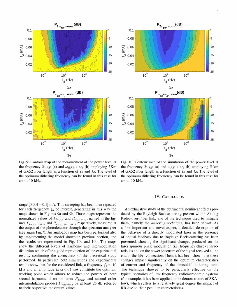
Fig. 8: Comparison between experimental and simulated val-ues of the modulating current amplitude Id which, for a givenmodulating frequency fd, determine the fixed value of thephase modulation index |Md| = 0.92.

As a preliminary test, the values of the dithering currentamplitude Id which lead to a maximum of the intermodulationterm at frequency ωRF+ωd, PωRF +ωd

have been measured forvarying values of fd. The behavior of this spurious componentis described by (33) considering nd = 1, nRF = 1 and itcan be shown that the value of current Id which gives themaximum of PωRF +ωd

is obtained when Md ' 0.92, which,with good approximation, corresponds to the value which givesthe maximum of

∑kmax

k=1 J21 (Xd,k). Figure 8 shows the good

agreement between simulated and measured values of Id.Note that this analysis have been performed considering

fd = 1 kHz as the lowest value of dithering frequency. Thereason behind this choice is that for lower frequencies it is notpossible to identify experimentally the maximum of PωRF +ωd

.After this preliminary test, an analysis of the behavior of

the terms P2ωRFand PωRF +ωd

as a function of Id and fd hasbeen experimentally performed.

The measurements have been conducted by fixing the valueof certain frequency fd and sweeping the current Id for a

9

P2

RF, norm

(dB)

102 104 106

fd (Hz)

0.02

0.04

0.06

0.08

0.1

I d (

mA

)

-25

-20

-15

-10

-5

0

(a)P

RF+

d, norm

(dB)

102 104 106

fd (Hz)

0.02

0.04

0.06

0.08

0.1

I d (

mA

)

-25

-20

-15

-10

-5

0

(b)

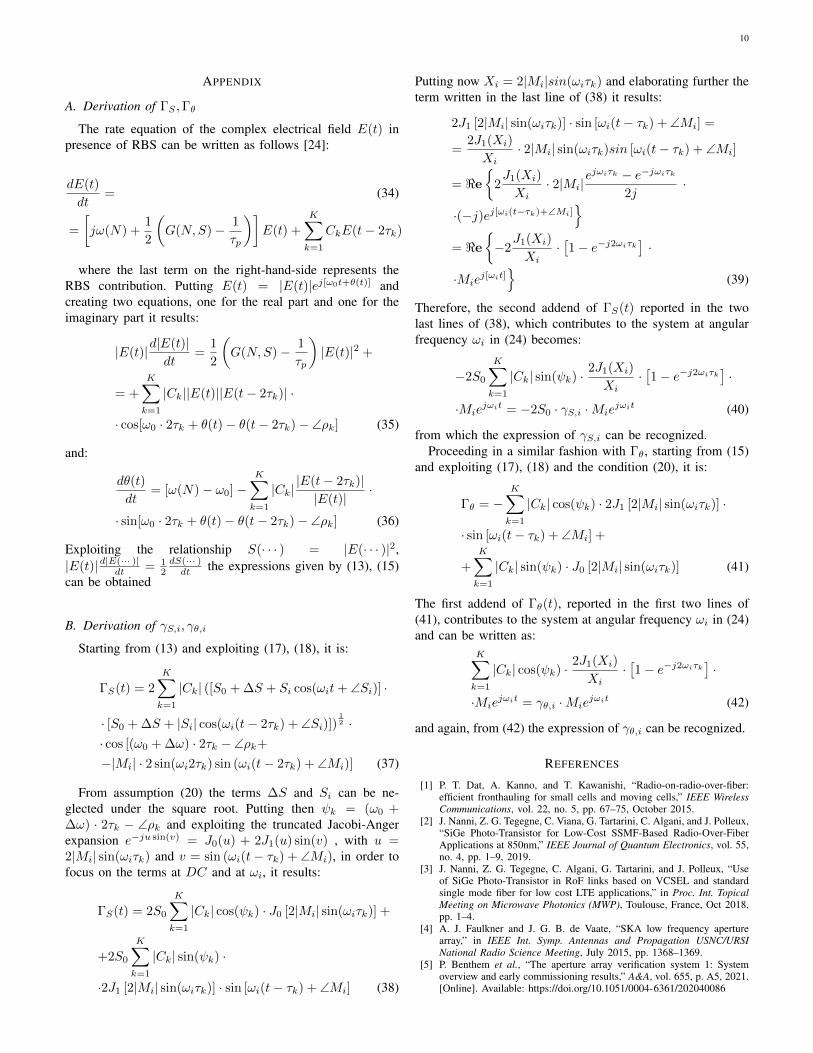
Fig. 9: Contour map of the measurement of the power level atthe frequency 2ωRF (a) and ωRFI + ωd (b) employing 5Kmof G.652 fiber length as a function of Id and fd. The level ofthe optimum dithering frequency can be found in this case forabout 10 kHz.

range [0.001−0.1] mA. This sweeping has been then repeatedfor each frequency fd of interest, generating in this way themaps shown in Figures 9a and 9b. Those maps represent thenormalized values of P2ωRF

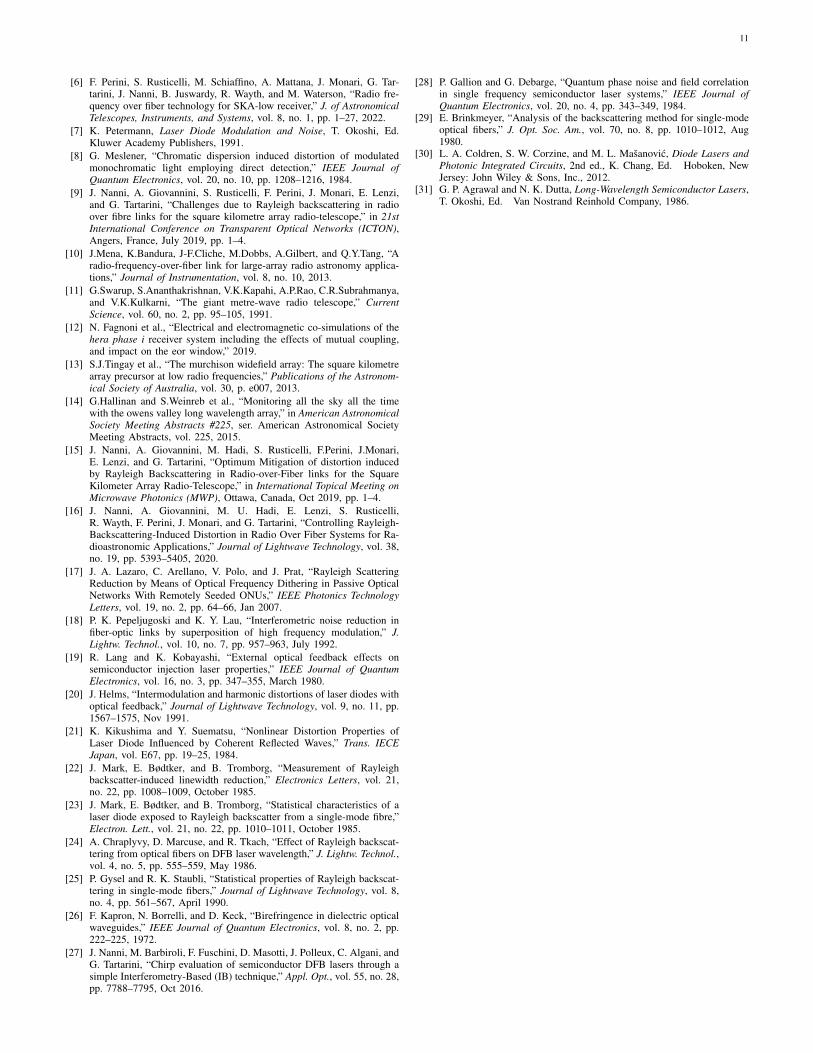
and PωRF +ωd, named in the fig-

ures P2ωRF ,norm and PωRF +ωd,norm respectively, measured atthe output of the photodetector through the spectrum analyzer(see again Fig.7). An analogous map has been performed alsoby implementing the model shown in previous section, andthe results are represented in Fig. 10a and 10b. The mapsshow the different levels of harmonic and intermodulationdistortion which offer a good reproduction of the experimentalresults, confirming the correctness of the theoretical studyperformed. In particular, both simulations and experimentalresults show that for the considered link, a frequency fd ' 10kHz and an amplitude Id ' 0.04 mA constitute the optimumworking point which allows to reduce the powers of bothsecond harmonic distortion term P2ωRF

and second orderintermodulation product PωRF +ωd

by at least 25 dB referredto their respective maximum values.

P2

RF, norm

(dB)

102 104 106

fd (Hz)

0.02

0.04

0.06

0.08

0.1

I d (

mA

)

-25

-20

-15

-10

-5

0

(a)P

RF+

d, norm

(dB)

102 104 106

fd (Hz)

0.02

0.04

0.06

0.08

0.1

I d (

mA

)

-25

-20

-15

-10

-5

0

(b)

Fig. 10: Contour map of the simulation of the power level atthe frequency 2ωRF (a) and ωRF + ωd (b) employing 5 kmof G.652 fiber length as a function of Id and fd. The level ofthe optimum dithering frequency can be found in this case forabout 10 kHz.

IV. CONCLUSION

An exhaustive study of the detrimental nonlinear effects pro-duced by the Rayleigh Backscattering present within AnalogRadio-over-Fiber link, and of the technique used to mitigatethem, namely the dithering technique, has been shown. Asa first important and novel aspect, a detailed description ofthe behavior of a directly modulated laser in the presenceof optical feedback due to Rayleigh Backscattering has beenpresented, showing the significant changes produced on thelaser spurious phase modulation (i.e. frequency chirp) charac-teristics and on the power spectrum of the signal received at theend of the fiber connection. Then, it has been shown that thesechanges impact significantly on the optimum characteristicsof current and frequency of the sinusoidal dithering tone.The technique showed to be particularly effective on thetypical scenarios of low frequency radioastronomic systems(for example, it has been applied in the demonstrators of SKA-low), which suffers to a relatively great degree the impact ofRB due to their peculiar characteristics.

10

APPENDIX

A. Derivation of ΓS ,Γθ

The rate equation of the complex electrical field E(t) inpresence of RBS can be written as follows [24]:

dE(t)

dt= (34)

=

[jω(N) +

1

2

(G(N,S)− 1

τp

)]E(t) +

K∑k=1

CkE(t− 2τk)

where the last term on the right-hand-side represents theRBS contribution. Putting E(t) = |E(t)|ej[ω0t+θ(t)] andcreating two equations, one for the real part and one for theimaginary part it results:

|E(t)|d|E(t)|dt

=1

2

(G(N,S)− 1

τp

)|E(t)|2 +

= +

K∑k=1

|Ck||E(t)||E(t− 2τk)| ·

· cos[ω0 · 2τk + θ(t)− θ(t− 2τk)− ∠ρk] (35)

and:

dθ(t)

dt= [ω(N)− ω0]−

K∑k=1

|Ck||E(t− 2τk)||E(t)|

·

· sin[ω0 · 2τk + θ(t)− θ(t− 2τk)− ∠ρk] (36)

Exploiting the relationship S(· · · ) = |E(· · · )|2,|E(t)|d|E(··· )|

dt = 12dS(··· )dt the expressions given by (13), (15)

can be obtained

B. Derivation of γS,i, γθ,i

Starting from (13) and exploiting (17), (18), it is:

ΓS(t) = 2

K∑k=1

|Ck| ([S0 + ∆S + Si cos(ωit+ ∠Si)] ·

· [S0 + ∆S + |Si| cos(ωi(t− 2τk) + ∠Si)])12 ·

· cos [(ω0 + ∆ω) · 2τk − ∠ρk+

−|Mi| · 2 sin(ωi2τk) sin (ωi(t− 2τk) + ∠Mi)] (37)

From assumption (20) the terms ∆S and Si can be ne-glected under the square root. Putting then ψk = (ω0 +∆ω) · 2τk − ∠ρk and exploiting the truncated Jacobi-Angerexpansion e−ju sin(v) = J0(u) + 2J1(u) sin(v) , with u =2|Mi| sin(ωiτk) and v = sin (ωi(t− τk) + ∠Mi), in order tofocus on the terms at DC and at ωi, it results:

ΓS(t) = 2S0

K∑k=1

|Ck| cos(ψk) · J0 [2|Mi| sin(ωiτk)] +

+2S0

K∑k=1

|Ck| sin(ψk) ·

·2J1 [2|Mi| sin(ωiτk)] · sin [ωi(t− τk) + ∠Mi] (38)

Putting now Xi = 2|Mi|sin(ωiτk) and elaborating further theterm written in the last line of (38) it results:

2J1 [2|Mi| sin(ωiτk)] · sin [ωi(t− τk) + ∠Mi] =

=2J1(Xi)

Xi· 2|Mi| sin(ωiτk)sin [ωi(t− τk) + ∠Mi]

= <e

2J1(Xi)

Xi· 2|Mi|

ejωiτk − e−jωiτk

2j·

·(−j)ej[ωi(t−τk)+∠Mi]

= <e−2

J1(Xi)

Xi·[1− e−j2ωiτk

]·

·Miej[ωit]

(39)

Therefore, the second addend of ΓS(t) reported in the twolast lines of (38), which contributes to the system at angularfrequency ωi in (24) becomes:

−2S0

K∑k=1

|Ck| sin(ψk) · 2J1(Xi)

Xi·[1− e−j2ωiτk

]·

·Miejωit = −2S0 · γS,i ·Mie

jωit (40)

from which the expression of γS,i can be recognized.Proceeding in a similar fashion with Γθ, starting from (15)

and exploiting (17), (18) and the condition (20), it is:

Γθ = −K∑k=1

|Ck| cos(ψk) · 2J1 [2|Mi| sin(ωiτk)] ·

· sin [ωi(t− τk) + ∠Mi] +

+

K∑k=1

|Ck| sin(ψk) · J0 [2|Mi| sin(ωiτk)] (41)

The first addend of Γθ(t), reported in the first two lines of(41), contributes to the system at angular frequency ωi in (24)and can be written as:

K∑k=1

|Ck| cos(ψk) · 2J1(Xi)

Xi·[1− e−j2ωiτk

]·

·Miejωit = γθ,i ·Mie

jωit (42)

and again, from (42) the expression of γθ,i can be recognized.

REFERENCES

[1] P. T. Dat, A. Kanno, and T. Kawanishi, “Radio-on-radio-over-fiber:efficient fronthauling for small cells and moving cells,” IEEE WirelessCommunications, vol. 22, no. 5, pp. 67–75, October 2015.

[2] J. Nanni, Z. G. Tegegne, C. Viana, G. Tartarini, C. Algani, and J. Polleux,“SiGe Photo-Transistor for Low-Cost SSMF-Based Radio-Over-FiberApplications at 850nm,” IEEE Journal of Quantum Electronics, vol. 55,no. 4, pp. 1–9, 2019.

[3] J. Nanni, Z. G. Tegegne, C. Algani, G. Tartarini, and J. Polleux, “Useof SiGe Photo-Transistor in RoF links based on VCSEL and standardsingle mode fiber for low cost LTE applications,” in Proc. Int. TopicalMeeting on Microwave Photonics (MWP), Toulouse, France, Oct 2018,pp. 1–4.

[4] A. J. Faulkner and J. G. B. de Vaate, “SKA low frequency aperturearray,” in IEEE Int. Symp. Antennas and Propagation USNC/URSINational Radio Science Meeting, July 2015, pp. 1368–1369.

[5] P. Benthem et al., “The aperture array verification system 1: Systemoverview and early commissioning results,” A&A, vol. 655, p. A5, 2021.[Online]. Available: https://doi.org/10.1051/0004-6361/202040086

11

[6] F. Perini, S. Rusticelli, M. Schiaffino, A. Mattana, J. Monari, G. Tar-tarini, J. Nanni, B. Juswardy, R. Wayth, and M. Waterson, “Radio fre-quency over fiber technology for SKA-low receiver,” J. of AstronomicalTelescopes, Instruments, and Systems, vol. 8, no. 1, pp. 1–27, 2022.

[7] K. Petermann, Laser Diode Modulation and Noise, T. Okoshi, Ed.Kluwer Academy Publishers, 1991.

[8] G. Meslener, “Chromatic dispersion induced distortion of modulatedmonochromatic light employing direct detection,” IEEE Journal ofQuantum Electronics, vol. 20, no. 10, pp. 1208–1216, 1984.

[9] J. Nanni, A. Giovannini, S. Rusticelli, F. Perini, J. Monari, E. Lenzi,and G. Tartarini, “Challenges due to Rayleigh backscattering in radioover fibre links for the square kilometre array radio-telescope,” in 21stInternational Conference on Transparent Optical Networks (ICTON),Angers, France, July 2019, pp. 1–4.

[10] J.Mena, K.Bandura, J-F.Cliche, M.Dobbs, A.Gilbert, and Q.Y.Tang, “Aradio-frequency-over-fiber link for large-array radio astronomy applica-tions,” Journal of Instrumentation, vol. 8, no. 10, 2013.

[11] G.Swarup, S.Ananthakrishnan, V.K.Kapahi, A.P.Rao, C.R.Subrahmanya,and V.K.Kulkarni, “The giant metre-wave radio telescope,” CurrentScience, vol. 60, no. 2, pp. 95–105, 1991.

[12] N. Fagnoni et al., “Electrical and electromagnetic co-simulations of thehera phase i receiver system including the effects of mutual coupling,and impact on the eor window,” 2019.

[13] S.J.Tingay et al., “The murchison widefield array: The square kilometrearray precursor at low radio frequencies,” Publications of the Astronom-ical Society of Australia, vol. 30, p. e007, 2013.

[14] G.Hallinan and S.Weinreb et al., “Monitoring all the sky all the timewith the owens valley long wavelength array,” in American AstronomicalSociety Meeting Abstracts #225, ser. American Astronomical SocietyMeeting Abstracts, vol. 225, 2015.

[15] J. Nanni, A. Giovannini, M. Hadi, S. Rusticelli, F.Perini, J.Monari,E. Lenzi, and G. Tartarini, “Optimum Mitigation of distortion inducedby Rayleigh Backscattering in Radio-over-Fiber links for the SquareKilometer Array Radio-Telescope,” in International Topical Meeting onMicrowave Photonics (MWP), Ottawa, Canada, Oct 2019, pp. 1–4.

[16] J. Nanni, A. Giovannini, M. U. Hadi, E. Lenzi, S. Rusticelli,R. Wayth, F. Perini, J. Monari, and G. Tartarini, “Controlling Rayleigh-Backscattering-Induced Distortion in Radio Over Fiber Systems for Ra-dioastronomic Applications,” Journal of Lightwave Technology, vol. 38,no. 19, pp. 5393–5405, 2020.

[17] J. A. Lazaro, C. Arellano, V. Polo, and J. Prat, “Rayleigh ScatteringReduction by Means of Optical Frequency Dithering in Passive OpticalNetworks With Remotely Seeded ONUs,” IEEE Photonics TechnologyLetters, vol. 19, no. 2, pp. 64–66, Jan 2007.

[18] P. K. Pepeljugoski and K. Y. Lau, “Interferometric noise reduction infiber-optic links by superposition of high frequency modulation,” J.Lightw. Technol., vol. 10, no. 7, pp. 957–963, July 1992.

[19] R. Lang and K. Kobayashi, “External optical feedback effects onsemiconductor injection laser properties,” IEEE Journal of QuantumElectronics, vol. 16, no. 3, pp. 347–355, March 1980.

[20] J. Helms, “Intermodulation and harmonic distortions of laser diodes withoptical feedback,” Journal of Lightwave Technology, vol. 9, no. 11, pp.1567–1575, Nov 1991.

[21] K. Kikushima and Y. Suematsu, “Nonlinear Distortion Properties ofLaser Diode Influenced by Coherent Reflected Waves,” Trans. IECEJapan, vol. E67, pp. 19–25, 1984.

[22] J. Mark, E. Bødtker, and B. Tromborg, “Measurement of Rayleighbackscatter-induced linewidth reduction,” Electronics Letters, vol. 21,no. 22, pp. 1008–1009, October 1985.

[23] J. Mark, E. Bødtker, and B. Tromborg, “Statistical characteristics of alaser diode exposed to Rayleigh backscatter from a single-mode fibre,”Electron. Lett., vol. 21, no. 22, pp. 1010–1011, October 1985.

[24] A. Chraplyvy, D. Marcuse, and R. Tkach, “Effect of Rayleigh backscat-tering from optical fibers on DFB laser wavelength,” J. Lightw. Technol.,vol. 4, no. 5, pp. 555–559, May 1986.

[25] P. Gysel and R. K. Staubli, “Statistical properties of Rayleigh backscat-tering in single-mode fibers,” Journal of Lightwave Technology, vol. 8,no. 4, pp. 561–567, April 1990.

[26] F. Kapron, N. Borrelli, and D. Keck, “Birefringence in dielectric opticalwaveguides,” IEEE Journal of Quantum Electronics, vol. 8, no. 2, pp.222–225, 1972.

[27] J. Nanni, M. Barbiroli, F. Fuschini, D. Masotti, J. Polleux, C. Algani, andG. Tartarini, “Chirp evaluation of semiconductor DFB lasers through asimple Interferometry-Based (IB) technique,” Appl. Opt., vol. 55, no. 28,pp. 7788–7795, Oct 2016.

[28] P. Gallion and G. Debarge, “Quantum phase noise and field correlationin single frequency semiconductor laser systems,” IEEE Journal ofQuantum Electronics, vol. 20, no. 4, pp. 343–349, 1984.

[29] E. Brinkmeyer, “Analysis of the backscattering method for single-modeoptical fibers,” J. Opt. Soc. Am., vol. 70, no. 8, pp. 1010–1012, Aug1980.

[30] L. A. Coldren, S. W. Corzine, and M. L. Masanovic, Diode Lasers andPhotonic Integrated Circuits, 2nd ed., K. Chang, Ed. Hoboken, NewJersey: John Wiley & Sons, Inc., 2012.

[31] G. P. Agrawal and N. K. Dutta, Long-Wavelength Semiconductor Lasers,T. Okoshi, Ed. Van Nostrand Reinhold Company, 1986.