Stud. Univ. Babe¸ s-Bolyai Math. 60(2015), No. 2, 151–171 Optimal cubic Lagrange interpolation: Extremal node systems with minimal Lebesgue constant Heinz-Joachim Rack and Robert Vajda Abstract. In the theory of interpolation of continuous functions by algebraic poly- nomials of degree at most n - 1 ≥ 2, the search for explicit analytic expressions of extremal node systems which lead to the minimal Lebesgue constant is still an intriguing topic in mathematics today [33]. The first non-trivial case n - 1=2 (quadratic interpolation) has been completely resolved, even in two alternative fashions, see [25], [27]. In the present paper we proceed to completely resolve the cubic case (n - 1 = 3) of optimal polynomial Lagrange interpolation on the unit interval [-1, 1]. We will provide two explicit analytic expressions for the uncount- able infinitely many extremal node systems x * 1 <x * 2 <x * 3 <x * 4 in [-1, 1] which all lead to the (known) minimal Lebesgue constant of cubic Lagrange interpola- tion on [-1, 1]. The descriptions of the extremal node systems (which need not be zero-symmetric) resemble the solutions for the quadratic case and incorporate two intrinsic constants expressed by radicals, of which one constant looks partic- ularly intricate. Our results encompass earlier related work provided in [17], [23], [24], [29], [30] and are guided by symbolic computation. Mathematics Subject Classification (2010): 05C35, 33F10, 41A05, 41A44, 65D05, 68W30. Keywords: Constant, cubic, extremal, interpolation, Lagrange interpolation, Lebesgue constant, minimal, node, node system, optimal, point, polynomial, sym- bolic computation. 1. Introduction Lagrange polynomial interpolation on node systems x 1 <x 2 < ··· <x n−1 <x n in some interval I is a classical and feasible method to approximate (continuous) func- tions on I by algebraic polynomials of maximal degree n - 1, see e.g. [9], [18], [21], This paper was presented at the third edition of the International Conference on Numerical Analysis and Approximation Theory (NAAT 2014), Cluj-Napoca, Romania, September 17-20, 2014.

Welcome message from author
This document is posted to help you gain knowledge. Please leave a comment to let me know what you think about it! Share it to your friends and learn new things together.
Transcript
Stud. Univ. Babes-Bolyai Math. 60(2015), No. 2, 151–171
Optimal cubic Lagrange interpolation:Extremal node systems with minimalLebesgue constant
Heinz-Joachim Rack and Robert Vajda
Abstract. In the theory of interpolation of continuous functions by algebraic poly-nomials of degree at most n− 1 ≥ 2, the search for explicit analytic expressionsof extremal node systems which lead to the minimal Lebesgue constant is still anintriguing topic in mathematics today [33]. The first non-trivial case n − 1 = 2(quadratic interpolation) has been completely resolved, even in two alternativefashions, see [25], [27]. In the present paper we proceed to completely resolve thecubic case (n− 1 = 3) of optimal polynomial Lagrange interpolation on the unitinterval [−1, 1]. We will provide two explicit analytic expressions for the uncount-able infinitely many extremal node systems x∗
1 < x∗
2 < x∗
3 < x∗
4 in [−1, 1] whichall lead to the (known) minimal Lebesgue constant of cubic Lagrange interpola-tion on [−1, 1]. The descriptions of the extremal node systems (which need notbe zero-symmetric) resemble the solutions for the quadratic case and incorporatetwo intrinsic constants expressed by radicals, of which one constant looks partic-ularly intricate. Our results encompass earlier related work provided in [17], [23],[24], [29], [30] and are guided by symbolic computation.
Mathematics Subject Classification (2010): 05C35, 33F10, 41A05, 41A44, 65D05,68W30.
Keywords: Constant, cubic, extremal, interpolation, Lagrange interpolation,Lebesgue constant, minimal, node, node system, optimal, point, polynomial, sym-bolic computation.
1. Introduction
Lagrange polynomial interpolation on node systems x1 < x2 < · · · < xn−1 < xn
in some interval I is a classical and feasible method to approximate (continuous) func-tions on I by algebraic polynomials of maximal degree n − 1, see e.g. [9], [18], [21],
This paper was presented at the third edition of the International Conference on Numerical Analysisand Approximation Theory (NAAT 2014), Cluj-Napoca, Romania, September 17-20, 2014.
152 Heinz-Joachim Rack and Robert Vajda
[26] or [28] for details. The goodness of this approximation method, as compared withthe best possible approximation in Chebyshev’s sense, is measured by means of theLebesgue constants which can be viewed as operator norms or condition numbers,see also [33]. They depend, for a given n, solely on the chosen configuration of in-terpolation points, and Lebesgue’s lemma suggests that we choose them in such amanner that the corresponding Lebesgue constant becomes least. Such extremal (or:optimal) node systems are in a sense the opposite to the equidistant interpolationpoints which may yield disastrous approximation results, see e.g. Runge’s examplein [18]. Although near-optimal node systems are known, and algorithms exist to nu-merically compute optimal (canonical) node systems, see [1] and [18], the search forexplicit analytic formulas characterizing optimal node systems remains an intriguingand challenging topic in mathematics today. Here are three quotations in this regard,see also [6], [7], [13], [14], [17], [33]:
• The nature of the optimal set X∗ remains a mystery [15, p. xlvii]• The problem of analytical description of the optimal matrix of nodes is consideredby pure mathematicians as a great challenge. [4]
• To this day there is no explicit representation for the nth row of the optimalarray, and in all likelihood there never will be. [16]
It suffices to restrict the search for optimal node systems to the unit interval I =[−1, 1]. The first non-trivial case n − 1 = 2 of quadratic Lagrange interpolation onI has been completely resolved: All optimal node systems x∗
1 < x∗2 < x∗
3 in I can beexplicitly described in two alternative fashions, see [25], [27]. In the present paper weproceed to completely resolve the cubic case n−1 = 3. Similarly to the quadratic casewe will provide two alternative, but equivalent, explicit analytic (i.e., non-numeric)descriptions of all extremal node systems x∗
1 < x∗2 < x∗
3 < x∗4 (with −1 ≤ x∗
1 andx∗4 ≤ 1) which, by their definition, lead to the (known) minimal Lebesgue constant
of cubic Lagrange interpolation on I. Amplifying Theorem 2 in [17] which statesthat optimal node systems are not unique, we will furthermore show that actuallythere exist, for each n − 1 ≥ 2, uncountable infinitely many such node systems inI. Generally, they are zero-asymmetrically distributed in I; however, the subset ofoptimal zero-symmetric node systems deserves special attention: The investigation, inthe cubic case, of optimal node systems −x∗
4 < −x∗3 < x∗
3 < x∗4 produces two intrinsic
constants (b and t, as defined below, of which b is particularly intricate) which are keyin describing the general distribution of all optimal node systems x∗
1 < x∗2 < x∗
3 < x∗4.
These can be geometrically visualized by a 2D-region in the plane spanned by the twoouter optimal nodes.
Historically, the first investigation into optimal node systems for the cubic caseseems to be [29, p. 229], [30, Problem 6.43], where an analytic, but implicit (i.e.,not by radicals) formula for the optimal zero-symmetric node systems as well as forthe minimal Lebesgue constant has been provided. However, the reader of [29], [30]might be left with the impression that actually all optimal node systems had beendetermined in this way, since optimal zero-asymmetric ones are not mentioned there.A particular case of a zero-symmetric node system in I (for n− 1 = 3) is a canonicalnode distribution −1 < −x3 < x3 < 1. The unique node x3 = x∗
3 = t which turns
Optimal cubic Lagrange interpolation 153
it to the optimal canonical node configuration has been explicitly determined in [23],[24], where also the minimal Lebesgue constant for the cubic Lagrange interpolationon I has been determined in an explicit form. Both quantities can be expressed,using Cardan’s formula, by means of roots of certain cubic polynomials with integercoefficients.
The manuscript is organized as follows: After providing some necessary notationsand definitions, we will consider, in an ascending order of generalization, first canon-ical node systems, then zero-symmetric node systems, and finally arbitrary (zero-symmetric and zero-asymmetric) node systems and will establish corresponding opti-mal node configurations. The proofs are postponed to section 6.
We hope that this paper, along with [25], [27] and our dedicated web repositorywww.math.u-szeged.hu/~vajda/Leb/ will add to the dissemination of computer-aided optimal quadratic and cubic Lagrange interpolation and may stimulate researchof the higher-degree polynomial cases, see Remark 7.5.
2. Definitions and basic theoretical background
Let C(I) denote the Banach space of continuous real functions f on I, equippedwith the uniform norm:
||f || = maxx∈I
|f(x)|. (2.1)
We wish to approximate f by an algebraic polynomial of degree at most n− 1, wheren ≥ 3. An old idea, named after Lagrange, see [19], is to sample f at n distinct pointsin I,
Xn : −1 ≤ x1 < x2 < . . . < xn−1 < xn ≤ 1, (2.2)
and to construct an interpolating polynomial of degree at most n− 1 as follows:
Ln−1(x) = Ln−1(f,Xn, x) =n∑
j=1
f(xj)ℓn−1,j(Xn, x) (2.3)
where
ℓn−1,j(x) = ℓn−1,j(Xn, x) =
n∏
i=1,i6=j
x− xi
xj − xi, (2.4)
so thatℓn−1,j(Xn, xi) = δj,i (Kronecker delta) (2.5)
and henceLn−1(xi) = f(xi), 1 ≤ i ≤ n (interpolatory condition) (2.6)
If ||f || ≤ 1 then (2.3) implies that |Ln−1(x)| can be estimated from above byn∑
j=1
|ℓn−1,j(Xn, x)| = λn(x) = λn(Xn, x). (2.7)
Definition 2.1. We call the xi’s in (2.2) the interpolation nodes and the grid Xn thenode system, the unique Ln−1 the Lagrange interpolation polynomial, the ℓn−1,j’s(of exact degree n− 1) the Lagrange fundamental polynomials, and λn the Lebesguefunction (named after Lebesgue, see [34]).
154 Heinz-Joachim Rack and Robert Vajda
Three properties of λn are summarized in the following statement, see [4], [17], [28,p. 95]:
Proposition 2.2.i) λn is a piecewise polynomial satisfying λn(x) ≥ 1 with equality only if x = xi
(1 ≤ i ≤ n).ii) λn has precisely one local maximum, which we will denote by µi = µi(Xn), in
each open sub-interval (xi, xi+1) of Xn (1 ≤ i ≤ n−1). The extremum point in(xi, xi+1), at which the maximum µi is attained, we will denote by ξi = ξi(Xn)so that λn(ξi) = µi holds.
iii) λn is strictly decreasing and convex in (−∞, x1) and strictly increasing andconvex in (xn,∞).
Definition 2.3. The largest value of λn in I, denoted by Λn = Λn(Xn), is called theLebesgue constant:
Λn = maxx∈I
λn(x). (2.8)
The importance of Λn in interpolation theory stems from the following inequality (“Er-ror Comparison Theorem”) which can be viewed as a version of Lebesgue’s lemma,but can also be proved directly [26, Theorem 4.1]:
||f − Ln−1|| ≤ (1 + Λn)||f − P ∗n−1||, (2.9)
where f ∈ C(I), and P ∗n−1 denotes the polynomial of best uniform approximation
to f out of the linear space of all algebraic polynomials of degree at most n − 1.Usually, P ∗
n−1 is much harder to determine than Ln−1, and of course there alwaysholds ||f − P ∗
n−1|| ≤ ||f −Ln−1||. The estimate (2.9), which is sharp for some f , tellsus that a small Lebesgue constant implies that the approximation to f by the Lagrangeinterpolation polynomial is nearly as good as the best uniform approximation to f bymeans of P ∗
n−1. Therefore, it is desirable to minimize Λn which can be achieved by astrategic placement of the interpolation nodes.It is known [26, p. 100] that for each n ≥ 3 there exists, in I, an extremal (or optimal)node system Xn = X∗
n : −1 ≤ x∗1 < x∗
2 < · · · < x∗n−1 < x∗
n ≤ 1 such that there holds
Λ∗n = Λn(X
∗n) ≤ Λn = Λn(Xn) for all possible choices of node systems Xn. (2.10)
Definition 2.4. The Lebesgue constant Λ∗n is called minimal.
It is furthermore known that for a given n ≥ 3 an extremal node system is not unique,see [17, Theorem 2], and there in particular exists an extremal node system whichincludes the endpoints of I as interpolation nodes, see [26, p. 100]. Obviously, allextremal node systems, for a given n, generate the same minimal Lebesgue constant.We take the opportunity to amplify [17, Theorem 2] in the following way:
Theorem 2.5. For each n ≥ 3 there exist uncountable infinitely many optimal nodesystems X∗
n : x∗1 < x∗
2 < · · · < x∗n−1 < x∗
n in I which all yield (2.10).
Definition 2.6. The construction of Ln−1(f,X∗n, x) is called optimal Lagrange poly-
nomial interpolation on I since it furnishes, for a given n, the minimal interpolationerror in the sense of (2.9).
Optimal cubic Lagrange interpolation 155
Definition 2.7. A node system which includes the endpoints of I as interpolation nodes(that is, x1 = −1 and xn = 1) is called a canonical node system (abbreviated CNS).
In answering a conjecture which goes back to [3], it was proved in [8] and in [14] thatthe following deep result holds true:
Proposition 2.8. If a Lebesgue function corresponding to a CNS Xn satisfies the so-called equioscillation property
µ1 = µ2 = . . . = µn−2 = µn−1, (2.11)
then Xn is an extremal node system, i.e. Xn = X∗n with Λn(X
∗n) = Λ∗
n.
Thus, the fulfillment of (2.11) is a sufficient condition for a CNS to be extremal.Actually, it was additionally proved that a CNS which satisfies (2.11) is unique andzero-symmetric, i.e., x∗
i = −x∗n−i+1 for 1 ≤ i ≤ n.
To the best of our knowledge, currently the optimal CNS Xn = X∗n : −1 = −x∗
n <−x∗
n−1 < · · · < x∗n−1 < x∗
n = 1 and the associated minimal Lebesgue constantΛ∗n = Λ(X∗
n) are explicitly known only if n = 3 (X∗3 : −1 < 0 < 1 and Λ∗
3 = 1.25, see[3], [25], [27] or [33]), or if n = 4 (see next section).
In the next three sections we will focus on cubic interpolation on I by the Lagrangeinterpolation polynomial L3, i.e., we set n = 4.
3. The optimal canonical node system and the minimal Lebesgueconstant for cubic Lagrange interpolation
We consider first optimal cubic Lagrange interpolation on a CNS. It must bezero-symmetric if it has to be extremal, so that the goal is to find, analytically andexplicitly, the unique node x3 = x∗
3 = t in X4 : −1 = −x4 < −x3 < x3 < x4 = 1which turns X4 into the unique extremal node system X∗
4 : −1 < −t < t < 1and to determine the associated minimal Lebesgue constant Λ∗
4 = Λ4(X∗4 ) for cubic
Lagrange interpolation on I. This problem, which is also addressed in [21, Example2.5.3] and [22, Exercise 4.10], has been solved in [23], [24] by means of roots of certaincubic polynomials with integer coefficients: The minimal Lebesgue constant, Λ∗
4, isthe unique real root of the polynomial
P ∗3 (x) = −11 + 53x− 93x2 + 43x3. (3.1)
This root can be explicitly expressed, with the aid of Cardan’s formula, as
Λ∗4 =
1
129
(
93+3
√
125172+11868√69+
3
√
125172−11868√69
)
(3.2)
= 1.4229195732 . . . . (3.3)
The square of the (unique positive) optimal node x∗3 = t is the unique real root of the
polynomial
Q∗3(x) = −1 + 2x+ 17x2 + 25x3. (3.4)
156 Heinz-Joachim Rack and Robert Vajda
Hence t itself can be explicitly expressed, with the aid of Cardan’s formula, as
t =1
5√3
√
√
√
√−17 +3
√
14699 + 1725√69
2+
3
√
14699− 1725√69
2(3.5)
= 0.4177913013 . . . , (3.6)
so that
X∗4 : −1 < −t < t < 1, with t from (3.5), (3.7)
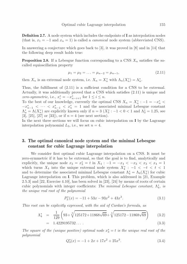
is the (unique and zero-symmetric) optimal CNS in I.Furthermore, also the three extremum points ξi = ξ∗i , with ξ∗1 = −ξ∗3 < ξ∗2 = 0 < ξ∗3 ,of the cubic Lebesgue function λ∗
4(x) = λ∗4(X
∗4 , x) are expressed in an analogous way
in [24], but we only provide here the numerical value ξ∗3 = 0.7331726239 . . . , seeFigure 1.
Figure 1
An analytical, but implicit, solution for t and Λ∗4 had been provided earlier in
[29, p. 229], [30, Problem 6.43], see also [23]: t is the unique positive root of thepolynomial
S6(x) = Q∗3(x
2) (3.8)
and
Λ∗4 =
1 + t2
1− t2. (3.9)
The polynomial (3.1) and the explicit expressions (3.2), (3.5) were not given there.Numerical values for t and/or Λ∗
4 are given, for example, in [1], [2], [4], [11], [20], [21]and [33].
4. Optimal zero-symmetric node systems for cubic Lagrangeinterpolation
We consider next optimal cubic Lagrange interpolation on zero-symmetric nodesystems in I.

Optimal cubic Lagrange interpolation 157
Problem 4.1. Find, analytically and explicitly, all optimal zero-symmetric node sys-tems X∗
4 : −x∗4 < −x∗
3 < x∗3 < x∗
4 in I !
Our solution to this problem will be expressed by means of the already deployedexplicit constant t according to (3.5) and by means of a real parameter β ∈ [1, b]where the right-hand endpoint b > 1 of that interval has still to be determined. Wewill first state our solution to Problem 4.1 and then turn to the task of determiningthe constant b.
Theorem 4.2. All optimal zero-symmetric node systems for the cubic Lagrange inter-polation on I are given by X∗
4 : −x∗4 < −x∗
3 < x∗3 < x∗
4, where
−x∗4 = − 1
β, −x∗
3 = − t
β, x∗
3 =t
β, x∗
4 =1
β. (4.1)
Here, t is given by (3.5) and β is an arbitrary number from the interval [1, b]. Theright-hand endpoint b > 1 of that interval will be specified implicitly and numericallyin Lemma 4.3, and explicitly in Lemma 4.4.
Note that the choice β = 1 takes us back to the optimal CNS as given in (3.7). For theconstant b in Theorem 4.2 we will now provide an implicit and an explicit analyticaldescription. However, both of them are intricate.
Lemma 4.3. The constant b in Theorem 4.2 can be expressed implicitly as the uniquepositive root of the following polynomial of degree 18 with integer coefficients:
P18(x) = −121 + 220x− 1014x2 + 1344x3 + 3283x4 − 5166x5 + 4502x6 (4.2)
+ 15692x7 − 84178x8 + 7868x9 + 210676x10 − 25694x11 − 310732x12
+ 34154x13 + 255377x14 − 8450x15 − 124700x16 + 26875x18.
The numerical evaluation of this root by computer algebra systems yields
b = 1.0433133411 . . . . (4.3)
However, the computer algebra systems we have checked do not render the real rootb of P18 by means of radicals. But such an explicit representation of b is possible:
Lemma 4.4. The constant b in Theorem 4.2 can be expressed explicitly in terms ofradicals as follows:
b = b(t) =
(
t+ t3
2 + 2t−√
(−1
27
)
(1 + (−1 + t)t)3 +(t+ t3)2
4(1 + t)2
)1/3
+
(
t+ t3
2 + 2t+
√
(−1
27
)
(1 + (−1 + t)t)3 +(t+ t3)2
4(1 + t)2
)1/3
, (4.4)
where t denotes the constant in (3.5), so that b still depends on t. Upon inserting thevalue (3.5) for t, one obtains in place of (4.4) a non-parametric explicit expression for
158 Heinz-Joachim Rack and Robert Vajda
b which, however, is quite intricate:
b =
((
58 +
(
1
2
(
14699− 1725√69)
)1/3
+
(
1
2
(
14699 + 1725√69)
)1/3)
(4.5)
/
(150+750√(
6/(
−34 + 22/3(
14699− 1725√69)1/3
+ 22/3(
14699+1725√69)1/3
)))
−√((58 21/3 +
(
14699− 1725√69)1/3
+(
14699 + 1725√69)1/3
)2/
(
3750 22/3(√
6 + 30/(√(−34 + 22/3
(
14699− 1725√69)1/3
+
22/3(
14699 + 1725√69)1/3
)))2)
−1
91125000
(
116 + 22/3(
14699− 1725√69)1/3
+ 22/3(
14699 + 1725√69)1/3 −
5√(
6(
−34 + 22/3(
14699− 1725√69)1/3
+
22/3(
14699 + 1725√69)1/3
)))3))1/3
+((
58 +(
12
(
14699− 1725√69))1/3
+(
12
(
14699 + 1725√69))1/3
)/
(150+750√(
6/(
−34 + 22/3(
14699− 1725√69)1/3
+ 22/3(
14699+1725√69)1/3
)))
+
√((58 21/3 +
(
14699− 1725√69)1/3
+(
14699 + 1725√69)1/3
)2/
(
3750 22/3(√
6 + 30/(√(−34 + 22/3
(
14699− 1725√69)1/3
+
22/3(
14699 + 1725√69)1/3
)))2)
−1
91125000
(
116 + 22/3(
14699− 1725√69)1/3
+ 22/3(
14699 + 1725√69)1/3 −
5√(
6(
−34 + 22/3(
14699− 1725√69)1/3
+ 22/3(
14699 + 1725√69)1/3
)))3))1/3
The first few decimal digits of b read, more precisely as in (4.3), as follows:
b = 1.043313341111592913631086831954493674798479469403995 . . . . (4.6)
To give an example, we consider the shortest sub-interval [−x∗4, x
∗4] of I which allows
optimal cubic Lagrange interpolation. According to Theorem 4.2 we have to chooseβ = b, so that we get, as a kind of counterpart to the CNS,
Example 4.5. The configuration
−x∗4 = −1
b, −x∗
3 = − t
b, x∗
3 =t
b, x∗
4 =1
b(4.7)
is the unique optimal zero-symmetric node system in I with the shortest intervallength x∗
4 − (−x∗4) =
2b . The corresponding numerical values are:
−0.9584848200 . . .<−0.4004466202 . . .<0.4004466202 . . .<0.9584848200 . . . (4.8)

Optimal cubic Lagrange interpolation 159
and2
b= 1.9169696400 . . . . (4.9)
We note that (4.7) is also unique in having the property that the correspondingLebesgue function λ4(x) equioscillates on I most, that is, five (= n + 1) times, seeFigure 2.
Figure 2
It is interesting to remark that the analogous configuration for the quadratic
case (n = 3) is − 2√2
3 < 0 < 2√2
3 , and the corresponding Lebesgue function λ3(x)equioscillates on I most, that is, four (= n + 1) times. The extremum points −1 <
−√23 <
√23 < 1 in I of that particular λ3(x) were considered by Bernstein in [3] and
motivated him to state his famous equioscillation conjecture. We therefore call (4.7)the Bernstein-type node system (BNS).
An analytical, but implicit, solution similar to (4.1) had been provided earlier in [29,p. 229] (misprinted) and [30, Problem 6.43]: The optimal zero-symmetric nodes in Iare −a < −at < at < 1, where a ∈ [a0, 1] and t is, as before, the unique positiveroot of the polynomial S6(x) = Q∗
3(x2) and a0 is the unique positive root of the
(parameterized) polynomial
S3(x) = −(t+ 1) + (t3 + 1)x2 + (t3 + t)x3. (4.10)
However, Tureckii did not express t and a0 by radicals, and in [29, p. 229] the term(t3+1)x2 of S3(x) was misprinted as (t3+1)x. We observe that the left-hand endpointa0 of the interval [a0, 1] coincides with
1b , where the constant b is given in Lemma 4.3
and 4.4. After all, we point out that optimal zero-asymmetric node systems are notmentioned in [29], [30], [31].
5. Optimal arbitrary node systems for cubic Lagrange interpolation
Finally we consider optimal cubic Lagrange interpolation on arbitrary (zero-symmetric and zero-asymmetric) node systems in I.
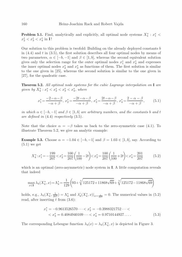
160 Heinz-Joachim Rack and Robert Vajda
Problem 5.1. Find, analytically and explicitly, all optimal node systems X∗4 : x∗
1 <x∗2 < x∗
3 < x∗4 in I !
Our solution to this problem is twofold: Building on the already deployed constants bin (4.4) and t in (3.5), the first solution describes all four optimal nodes by means oftwo parameters, α ∈ [−b,−1] and β ∈ [1, b], whereas the second equivalent solutiongives only the selection range for the outer optimal nodes x∗
1 and x∗4 and expresses
the inner optimal nodes x∗2 and x∗
3 as functions of them. The first solution is similarto the one given in [25], whereas the second solution is similar to the one given in[27], for the quadratic case.
Theorem 5.2. All optimal node systems for the cubic Lagrange interpolation on I aregiven by X∗
4 : x∗1 < x∗
2 < x∗3 < x∗
4, where
x∗1=
−2−α−β
−α+ β, x∗
2=−2t−α−β
−α+ β, x∗
3=2t−α−β
−α+ β, x∗
4=2− α− β
−α+ β, (5.1)
in which α ∈ [−b,−1] and β ∈ [1, b] are arbitrary numbers, and the constants b and tare defined in (4.4) respectively (3.5).
Note that the choice α = −β takes us back to the zero-symmetric case (4.1). Toillustrate Theorem 5.2, we give an analytic example:
Example 5.3. Choose α = −1.04 ∈ [−b,−1] and β = 1.03 ∈ [1, b], say. According to(5.1) we get
X∗4 :x
∗1=−199
207<x∗
2=100
207
(
1
100−2t
)
<x∗3=
100
207
(
1
100+2t
)
<x∗4=
201
207(5.2)
which is an optimal (zero-asymmetric) node system in I. A little computation revealsthat indeed
maxx∈I
λ4(X∗4 , x)=Λ∗
4=1
129
(
93+3
√
125172+11868√69+
3
√
125172−11868√69
)
holds, e.g., λ4(X∗4 ,
1207 ) = Λ∗
4 and λ′4(X
∗4 , x)|x= 1
207
= 0. The numerical values in (5.2)
read, after inserting t from (3.6):
x∗1 = −0.9613526570 · · ·< x∗
2 = −0.3988321752 · · ·<< x∗
3 = 0.4084940109 · · ·< x∗4 = 0.9710144927 . . . . (5.3)
The corresponding Lebesgue function λ4(x) = λ4(X∗4 , x) is depicted in Figure 3.

Optimal cubic Lagrange interpolation 161
Figure 3
Our second solution to Problem 5.1 likewise builds on the deployed constants b in(4.4) and t in (3.5). The two parameters α and β and their selection ranges are nowsuperseded by selection ranges for the two outer optimal nodes which, once fixed,uniquely determine the corresponding two inner optimal nodes.
Theorem 5.4. (Alternative solution to Problem 5.1) All optimal node systems for thecubic Lagrange interpolation on I are given by X∗
4 : x∗1 < x∗
2 < x∗3 < x∗
4, where either
−1 ≤ x∗1≤−1
b=−0.9584848200 . . . and
(
b− 1
b+ 1
)
x∗1+
2
b+ 1≤x∗
4≤1 (5.4)
or
−1
b<x∗
1≤b− 3
b+ 1=−0.9576047978 . . . and
(
b+ 1
b− 1
)
x∗1+
2
b− 1≤x∗
4≤1 (5.5)
with
x∗2 =
(
1 + t
2
)
x∗1 +
(
1− t
2
)
x∗4, (5.6)
and with
x∗3 =
(
1− t
2
)
x∗1 +
(
1 + t
2
)
x∗4. (5.7)
When the outer optimal nodes x∗1 and x∗
4 vary in their respective ranges (5.4) and(5.5), then also the ranges of the inner optimal nodes x∗
2 and x∗3 are exhausted. That
ranges are substantiated in the next statement.
Theorem 5.5. The two inner optimal nodes x∗2 and x∗
3 in Theorem 5.4 may vary withinthe ranges
−1
b+ 1(2t+b−1)=−0.4301327291 . . .≤x∗
2≤−1
b+ 1(2t−b+1)=−0.3877375269 . . . (5.8)
and
1
b+ 1(2t− b+1)=0.3877375269 · · · ≤x∗
3≤1
b+ 1(2t+ b− 1)=0.4301327291 . . . (5.9)
162 Heinz-Joachim Rack and Robert Vajda
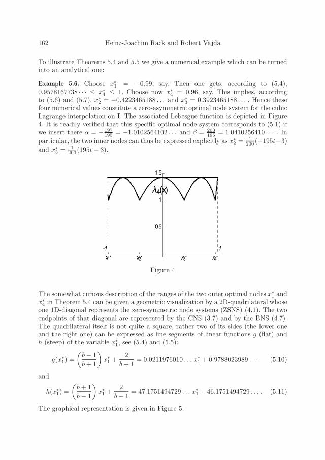
To illustrate Theorems 5.4 and 5.5 we give a numerical example which can be turnedinto an analytical one:
Example 5.6. Choose x∗1 = −0.99, say. Then one gets, according to (5.4),
0.9578167738 · · · ≤ x∗4 ≤ 1. Choose now x∗
4 = 0.96, say. This implies, accordingto (5.6) and (5.7), x∗
2 = −0.4223465188 . . . and x∗3 = 0.3923465188 . . . . Hence these
four numerical values constitute a zero-asymmetric optimal node system for the cubicLagrange interpolation on I. The associated Lebesgue function is depicted in Figure4. It is readily verified that this specific optimal node system corresponds to (5.1) ifwe insert there α = − 197
195 = −1.0102564102 . . . and β = 203195 = 1.0410256410 . . . . In
particular, the two inner nodes can thus be expressed explicitly as x∗2 = 1
200 (−195t−3)
and x∗3 = 1
200 (195t− 3).
Figure 4
The somewhat curious description of the ranges of the two outer optimal nodes x∗1 and
x∗4 in Theorem 5.4 can be given a geometric visualization by a 2D-quadrilateral whose
one 1D-diagonal represents the zero-symmetric node systems (ZSNS) (4.1). The twoendpoints of that diagonal are represented by the CNS (3.7) and by the BNS (4.7).The quadrilateral itself is not quite a square, rather two of its sides (the lower oneand the right one) can be expressed as line segments of linear functions g (flat) andh (steep) of the variable x∗
1, see (5.4) and (5.5):
g(x∗1) =
(
b− 1
b+ 1
)
x∗1 +
2
b+ 1= 0.0211976010 . . . x∗
1 + 0.9788023989 . . . (5.10)
and
h(x∗1) =
(
b+ 1
b− 1
)
x∗1 +
2
b− 1= 47.1751494729 . . . x∗
1 + 46.1751494729 . . . . (5.11)
The graphical representation is given in Figure 5.

Optimal cubic Lagrange interpolation 163
Figure 5
We are not aware of any published studies that provide explicit analytical solutionsto the problem of determining all optimal node systems in the frame of optimalpolynomial Lagrange interpolation on I with polynomials of degree ≥ 4 (i.e., n ≥ 5),notwithstanding that this large project is vibrant, see [5], and also Remark 7.5 below.The results for the polynomial degree = 3 as obtained in [23], [24], and [30, Problem6.43] do not cover zero-asymmetric node systems. Thus the present paper seems tobe the first one where, for the polynomial degree = 3, all optimal node systems in Ihave been determined, explicitly and analytically. For the polynomial degree = 2 thishas been achieved in [25] and in [27].
6. Proofs
6.1. Proof of Theorem 2.5
Proof. Let λ∗n(x) = λ∗
n(X∗n, x) denote the Lebesgue function corresponding to the
optimal CNS X∗n : −1 = −x∗
n = x∗1 < −x∗
n−1 = x∗2 < · · · < x∗
n−1 < x∗n = 1 in
I. We know that λ∗n(±1) = 1 and that λ∗
n(x) is strictly decreasing resp. increasingin (−∞,−1) and (1,∞), see Proposition 2.2. As Λ∗
n > 1, there exist unique valuesx = cn < −1 resp. x = bn > 1 with the property λ∗
n(cn) = λ∗n(bn) = Λ∗
n. Hence,maxx∈[cn,bn] λ
∗n(x) = Λ∗
n and in particular maxx∈[α,β] λ∗n(x) = Λ∗
n for any subinterval[α, β] of [cn, bn] which covers I. Choose now an arbitrary α ∈ [cn,−1] and an arbitraryβ ∈ [1, bn] and consider the linear transformation
S(x) =1
−α+ β(2x− α− β) (6.1)
which maps [α, β] onto I, because S(α) = −1 and S(β) = 1. In particular, the nodesof the optimal CNS X∗
n (which is contained in [α, β]) will be mapped as follows:

164 Heinz-Joachim Rack and Robert Vajda
S(−1) = y∗1 =1
−α+ β(−2− α− β)
S(−x∗n−1) = y∗2 =
1
−α+ β(−2x∗
n−1 − α− β)
. . .
S(x∗n−1) = y∗n−1 =
1
−α+ β(2x∗
n−1 − α− β)
S(1) = y∗n =1
−α+ β(2− α− β). (6.2)
As S(x) has the positive slope 2−α+β , these images are ordered ascendingly in I:
Y ∗n = Y ∗
n,α,β : y∗1 < y∗2 · · · < y∗n−1 < y∗n. (6.3)
We proceed to show that Y ∗n is an extremal node system (with minimal Lebesgue
constant) in I. To this end, we observe that, for y ∈ I and x ∈ [α, β], we have
λn(Y∗n , y) =
n∑
j=1
n∏
i=1
i6=j
|y − y∗i ||y∗j − y∗i |
=
n∑
j=1
n∏
i=1
i6=j
|S(x)− S(x∗i )|
|S(x∗j )− S(x∗
i )|=
=n∑
j=1
n∏
i=1
i6=j
| 1−α+β (2x−α−β)− 1
−α+β (2x∗i −α−β)|
| 1−α+β (2x
∗j−α−β)− 1
−α+β (2x∗i −α−β)|=
n∑
j=1
n∏
i=1
i6=j
|x− x∗i |
|x∗j − x∗
i |=
= λ∗n(x), (6.4)
and hence
maxy∈I
λn(Y∗n , y) = max
x∈[α,β]λ∗n(x) = Λ∗
n,
see also [21, Theorem 2.5.3] and [6, Problem 1, p. 22]. Thus, Y ∗n = Y ∗
n,α,β is indeedan optimal node system in I, and since α and β were chosen arbitrarily, there existuncountable infinitely many such Y ∗
n ’s. �
6.2. Proof of Theorem 4.2
Proof. The statement is a corollary to Theorem 5.2: insert there α = −β. �
6.3. Proof of Theorem 5.2
Proof. The Lebesgue function λ∗4(x) = λ∗
4(X∗4 , x) which corresponds to the optimal
CNS X∗4 in (3.7) is readily found to be given by
λ∗4(x) = |ℓ31(x)| + |ℓ32(x)|+ |ℓ33(x)| + |ℓ34(x)| = (6.5)
= |(−t− x)(−1 + x)(−t+ x)/(2(−1− t)(−1 + t))|+|(−1 + x)(1 + x)(−t+ x)/(2(−1− t)(1 − t)t)|+|(−1 + x)(1 + x)(t+ x)/(2(−1 + t)t(1 + t))|+|(1 + x)(−t+ x)(t+ x)/(2(1 − t)(1 + t))|,
where t is defined in (3.5).

Optimal cubic Lagrange interpolation 165
For x ∈ (1,∞), λ∗4(x) is strictly increasing and is representable there as
λ∗4(x) = −ℓ31(x) + ℓ32(x) − ℓ33(x) + ℓ34(x) =
x(1 − t+ t2 − x2)
(−1 + t)t. (6.6)
Let x = b > 1 denote the unique point on the x-axis where λ∗4(x) intercepts with the
constant function f(x) = Λ∗4, see (3.2). A numerical solution of the equation λ∗
4(x)−Λ∗4 = 0 is the value b given in (4.3). The expression of b as explicit analytical solution
we will provide below (see the proof of Lemma 4.4). Similarly, for x ∈ (−∞,−1),λ∗4(x) is strictly decreasing and is representable there as
λ∗4(x) = ℓ31(x) − ℓ32(x) + ℓ33(x) − ℓ34(x) =
x(−1 + t− t2 + x2)
(−1 + t)t, (6.7)
so that x = −b < −1 denotes the unique point on the x-axis where λ∗4(x) inter-
cepts with the constant function f(x) = Λ∗4. Thus we have, on the interval [−b, b]
as well as on any subinterval [α, β] thereof which covers I, maxx∈[−b,b] λ∗4(x) = Λ∗
4 =maxx∈I λ
∗4(x). We now apply the linear transformation (6.1) to X∗
4 in (3.7) with ar-bitrary α ∈ [−b,−1] and arbitrary β ∈ [1, b], and thus get (5.1), after renaming y∗i tox∗i , i = 1, 2, 3, 4 (see the proof of Theorem 2.5). In this way we generate uncountable
infinitely many extremal node systems x∗1 < x∗
2 < x∗3 < x∗
4 in I, and in fact we soobtain all extremal node systems in I.
For let X04 : x0
1 < x02 < x0
3 < x04 be an arbitrary extremal node system in I. The linear
transformation T (x) =2x−x0
1−x0
4
−x0
1+x0
4
maps X04 onto I since T (x0
1) = −1 and T (x04) = 1.
Since its slope 2−x0
1+x0
4
is positive, the mapped values are ordered ascendingly, that
is X04,T : −1 = T (x0
1) < T (x02) < T (x0
3) < T (x04) = 1, and hence X0
4,T is a CNS in
I. The Lebesgue constant corresponding to X04 (which equals Λ∗
4 as given in (3.2)) isidentical with the one corresponding to X0
4,T , see the proof of Theorem 2.5 or [21,
Theorem 2.5.3] or [6, Problem 1, p. 22]. But this implies that X04,T is necessarily the
unique CNS X∗4 on I, as given in (3.7). In particular we thus have T (x0
2) = −t andT (x0
3) = t, and this implies, by the definition of T (x), x02 =
(
1+t2
)
x01 +
(
1−t2
)
x04 and
x03 =
(
1−t2
)
x01 +
(
1+t2
)
x04, where t is from (3.5).
With this information at hand we proceed as follows: The linear transformation S from
(6.1) with α = α0 =−2−x0
4−x0
1
x0
4−x0
1
and β = β0 =2−x0
4−x0
1
x0
4−x0
1
maps the optimal CNS X∗4 onto
x01 < x0
2 < x03 < x0
4. Indeed, S(−1) = x01 and S(1) = x0
4 as is immediately verified.Furthermore we get S(−t) =
(
1+t2
)
x01+(
1−t2
)
x04 and S(t) =
(
1−t2
)
x01+(
1+t2
)
x04, and
these values are identical with x02 and x0
3 as shown above.
It remains to show that α0 ∈ [−b,−1] and β0 ∈ [1, b]. We will prove it by symboliccomputation employing the built-in language symbols InterpolatingPolynomial andResolve in Mathematica R© as well as Mathematica R©-specific notation. Furthermore,we will use the fact that λn(±1) ≤ Λ∗
n, see Proposition 2.2. Assume that the variableLF contains the Lebesgue function corresponding to the node system in (5.1). Thiscan be defined e.g. in Mathematica R© as follows:

166 Heinz-Joachim Rack and Robert Vajda
LF=Abs[InterpolatingPolynomial[{{x1[α, β], 1}, {x2[α, β], 0}, {x3[α, β], 0}, {x4[α, β], 0}}, x]] +Abs[InterpolatingPolynomial[{{x1[α, β], 0}, {x2[α, β], 1}, {x3[α, β], 0}, {x4[α, β], 0}}, x]] +Abs[InterpolatingPolynomial[{{x1[α, β], 0}, {x2[α, β], 0}, {x3[α, β], 1}, {x4[α, β], 0}}, x]] +Abs[InterpolatingPolynomial[{{x1[α, β], 0}, {x2[α, β], 0}, {x3[α, β], 0}, {x4[α, β], 1}}, x]].
Denote the the specific parameter values α0 and β0 by
α0 =−2− x4− x1
x4− x1β0 =
2− x4− x1
x4 − x1. (6.8)
Then one gets, with Λ = Λ∗4 as given in (3.2) and (3.9) and b as given in (4.2) and
(4.5),[in:]
Resolve[ForAll[{x1, x4}, (−1 ≤ x1 < x4 ≤ 1∧(LF/.x → −1) ≤ Λ ∧ (LF/.x → 1) ≤ Λ/.{α → α0, β → β0})⇒(−b ≤ α0 ≤ −1 ∧ 1 ≤ β0 ≤ b)],Reals] (6.9)
[out:] True. �
6.4. Proof of Lemma 4.3
Proof. We want to determine the point x = b > 1 on the x-axis where λ∗4(x) intercepts
with the constant function f(x) = Λ∗4 (see the proof of Theorem 5.2). To this end,
we employ a computer algebra system. The built-in language symbol RootReduceof Mathematica R© immediately gives, in view of (3.1), (3.4) and (6.6), the claimedpolynomial of degree 18:
[in:]
RootReduce[x/.Solve[x(1− t+ t2 − x2)/((−1 + t)t) ==
Root[−11 + 53#1− 93#12 + 43#13&, 1]
/.t → Root[−1 + 2#12 + 17#14 + 25#16&, 2], x,Reals]] (6.10)
[out:]
{Root[−121 + 220#1− 1014#12 + 1344#13 + 3283#14 − 5166#15+
4502#16 + 15692#17 − 84178#18 + 7868#19 + 210676#110−25694#111 − 310732#112 + 34154#113 + 255377#114−8450#115 − 124700#116 + 26875#118&, 2]}. (6.11)
This polynomial P18 can also be deduced in a reverse way: If one employs inMathematica R© the built-in language symbol FullSimplify to the explicit expression(4.5), then one gets (6.11). �
Optimal cubic Lagrange interpolation 167
6.5. Proof of Lemma 4.4
Proof. The equation
x(1 − t+ t2 − x2)/((−1 + t)t) =1 + t2
1− t2(6.12)
see (3.9) and (6.6), amounts to the following cubic algebraic equation in x:
(t+ t3) + (1 + t3)x+ (−1− t)x3 = 0. (6.13)
Solving (6.13) with the aid of Cardan’s formula yields the (parametric) solutionx = b = b(t) as given in (4.4). Inserting then into (4.4) the value for the constant taccording to (3.5) and simplifying eventually gives (4.5). The said algebraic manipu-lations can be executed by pencil and paper, but it is more convenient to guide themby a computer algebra system. �
6.6. Proof of Theorem 5.4
Proof. To prove (5.4) and (5.5), we use quantifier elimination to eliminate the existen-tially quantified variables α and β from the parametric representation of x∗
1 = x∗1(α, β)
and x∗4 = x∗
4(α, β), taking into account the range of α and β, see Theorem 5.2. Thiselimination can be executed by means of the built-in language symbol Resolve inMathematica R©:
[in :]
Resolve[Exists[{α, β},(
b > 1 ∧ −b ≤ α ≤ −1 ∧ 1 ≤ β ≤ b∧x∗1(β − α) == −2−α−β ∧ x∗
4(β − α) == 2−α−β)
], {x∗1, x
∗4},Reals]
[out :]
b > 1 ∧(
(−1 ≤ x∗1 ≤ −1
b∧ 2− x∗
1 + bx∗1
1 + b≤ x∗
4 ≤ 1)∨
(−1
b< x∗
1 ≤ −3 + b
1 + b∧ 2 + x∗
1 + bx∗1
−1 + b≤ x∗
4 ≤ 1))
, (6.14)
which coincides with (5.4) and (5.5). To prove (5.6) and (5.7), consider the parametricrepresentation of the optimal nodes x∗
i = x∗i (α, β), i = 1, 2, 3, 4 in (5.1). Computing
now(
1+t2
)
x∗1(α, β) +
(
1−t2
)
x∗4(α, β) and
(
1−t2
)
x∗1(α, β) +
(
1+t2
)
x∗4(α, β) gives imme-
diately (5.6) and (5.7). �
6.7. Proof of Theorem 5.5
Proof. According to (5.7), the node x∗3 = x∗
3(x∗1, x
∗4) =
(
1−t2
)
x∗1 +
(
1+t2
)
x∗4 is a bi-
variate polynomial which is linear in both variables x∗1 and x∗
4. Hence x∗3(x
∗1, x
∗4) will
attain its extreme values on the boundary of the ranges of x∗1 and x∗
4, so that it sufficesto investigate the values of x∗
3(x∗1, x
∗4) at five points, see (5.4), (5.5) and also Figure 5:
x∗3
(
−1,3− b
b+ 1
)
=2t− b + 1
b+ 1= 0.3877375269 . . . (6.15)
x∗3(−1, 1) = t = 0.4177913013 . . . (6.16)
x∗3
(−1
b,1
b
)
=t
b= 0.4004466202 . . . (6.17)
168 Heinz-Joachim Rack and Robert Vajda
x∗3
(−1
b, 1
)
=−1 + b + bt+ t
2b= 0.4298765508 . . . (6.18)
x∗3
(
b− 3
b− 1, 1
)
=2t+ b− 1
b+ 1= 0.4301327291 . . . . (6.19)
Obviously, (6.15) is the minimum and (6.19) is the maximum of x∗3 = x∗
3(x∗1, x
∗4) as
claimed in (5.9). The verification of (5.8) follows similar lines and will be left to thereader. �
7. Concluding remarks
Remark 7.1. Let n = 4. According to (4.7), the largest possible value for the firstoptimal interpolation node in I is x∗
1 = − 1b = −0.9584848200 . . . , if we consider zero-
symmetric node systems. But if we allow arbitrary node configurations, then we canget beyond this number: the largest possible value for the first optimal interpolationnode in I is in fact x∗
1 = b−3b+1 = −0.9576047978 . . . , see (5.5).
Remark 7.2. According to section 6.6, Schurer’s description in [27, Theorem 1] ofthe optimal arbitrary node systems X∗
3 : x∗1 < x∗
2 < x∗3 for quadratic Lagrange
interpolation on I can be restated almost verbatim in the form as given in our Theorem5.4, if we replace in (5.4) and (5.5) x∗
4 by x∗3 and if we replace the constant b =
1.0433133411 . . . by the corresponding constant b◦ = 32√2= 1.0606601717 . . . . For
example, (5.4) would then read
−1 ≤ x∗1 ≤ − 1
b◦(≈−0.9428) ∧
(
b◦ − 1
b◦ + 1
)
x∗1 +
2
b◦ + 1≤ x∗
3 ≤ 1 (7.1)
which is identical with
−1 ≤ x∗1 ≤ −2
√2
3(≈−0.9428) ∧ (17− 12
√2)x∗
1 + 12√2− 16 ≤ x∗
3 ≤ 1 (7.2)
as given in [27]. Note that in the quadratic case we have x∗2 =
x∗1+x∗
3
2 .
Remark 7.3. The proof of Theorem 5.4 rests on Theorem 5.2. We have also foundan alternative, computer-aided proof of Theorem 5.4 which avoids Theorem 5.2. Ituses quantifier elimination and can be compared with section 3.5 in [25]. However,to reduce computational complexity, this automated proof requires a reduction of thevariables by means of
x∗2 = x∗
1 + x∗4 − x∗
3. (7.3)
This equation, which is of some interest in itself, follows readily from Theorem 5.2,but, to stay independent of that theorem, we had to establish an alternative new prooffor (7.3).
Remark 7.4. Suppose one chooses x∗1 = c (constant) and x∗
4 = d (constant) from theindicated ranges (5.4) respectively (5.5) in Theorem 5.4. Then one gets, in generalizing
Example 5.6, α = −2−c−dd−c and β = 2−c−d
d−c , and hence x∗2 = c+d+t(c−d)
2 and x∗3 =
c+d+t(d−c)2 , according to Theorem 5.2, or directly from (5.6) and (5.7).

Optimal cubic Lagrange interpolation 169
Remark 7.5. The natural question arises: How to determine the minimal Lebesgueconstant Λ∗
n and all optimal node systems X∗n in I for the next cases n = 5, 6, 7, . . . ?
We have achieved some progress for n = 5 and n = 6. For example, we have implicitlydetermined the Lebesgue constants Λ∗
5 and Λ∗6 by symbolic computation as roots
of certain high-degree polynomials with integer coefficients. To be more specific, forn = 5 (quartic case) we have obtained
Λ∗5 = 1.5594902098 . . . (7.4)
as a root of a polynomial of degree 73 with integer coefficients. This polynomial hasthe contour
P ∗73(x) = (7.5)
491920844066918518676932058679834515105631225977247880376611328125 + . . .
+14156651510438131445849849962417864414147142283963792181670336004096 x73.
We intend to expose our findings in a separate manuscript, see also [32].
Remark 7.6. That the topic of optimal cubic Lagrange interpolation awakens interestin the reader may be deduced from the fact that the online-version of [23] on thepublishers website has received more than 60 article views subject to charge, seehttp://www.tandfonline.com/doi/abs/10.1080/0020739840150312
Remark 7.7. The desire to precisely determine the values of interesting constants(here: b, t, Λ∗
4) is reflected on in [12, p. 79].
Remark 7.8. In [10, p. 70] it is erroneously claimed that an optimal node system inI must necessarily be a CNS.
References
[1] Angelos, J.A., Kaufman, E.H. Jr., Henry, M.S., Lenker, T.D., Optimal nodes for poly-nomial interpolation, in: Approximation Theory VI, Vol. I, C.K. Chui, L.L. Schumaker,J.D. Ward (Eds.), (College Station, TX, 1989), 17-20, Academic Press, Boston, MA,1989.
[2] Babuska, I., Strouboulis, Th., The finite element method and its reliability, Oxford Uni-versity Press, Oxford, UK, 2001.
[3] Bernstein, S., Sur la limitation des valeurs d’un polynome Pn(x) de degre n sur toutun segment par ses valeurs en (n+ 1) points du segment, (in French), Izv. Akad. Nauk.SSSR, 7(1931), 1025-1050.
[4] Brutman, L., Lebesgue functions for polynomial interpolation – a survey, Ann. Numer.Math., 4(1997), 111-127.
[5] Chen, D., Generalization of polynomial interpolation at Chebyshev nodes, in: Approx-imation Theory XIII, M. Neamtu, L.L. Schumaker (Eds.), (San Antonio, TX, 2010),17-35, Springer Proc. Math. 13, Springer, New York, 2012.
[6] Cheney, E.W., Light, W.A., A course in approximation theory, AMS Publishing, Prov-idence, RI, 2000.
[7] Cheney, E.W., Xu, Y., A set of research problems in approximation theory, in: Topics inpolynomials of one and several variables and their applications, Th. M. Rassias, H.M.Srivastava, A. Yanushauskas (Eds.), 109-123, World Sci. Publ., River Edge, NJ, 1993.

170 Heinz-Joachim Rack and Robert Vajda
[8] de Boor, C., Pinkus, A., Proof of the conjectures of Bernstein and Erdos concerning theoptimal nodes for polynomial interpolation, J. Approx. Theory, 24(1978), 289-303.
[9] de Villiers, J., Mathematics of approximation, Atlantis Press, Paris, 2012.
[10] Dzyadyk, V.K., Approximation methods for solutions of differential and integral equa-tions, VSP, Utrecht, NL, 1995.
[11] Ehm, W., Beitrage zur Theorie optimaler Interpolationspunkte, (in German), DoctoralDissertation, Universitat Munster, 1977.
[12] Glaisher, J.W.L., Logarithms and computation, The Napier Tercentenary (Napier Ter-centenary Memorial Volume), C.G. Knott (Ed.), Longmans, Green & Co., London, 1915.
[13] Henry, M.S., Approximation by polynomials: Interpolation and optimal nodes, Am. Math.Mon., 91(1984), 497-499.
[14] Kilgore, Th.A., A characterization of the Lagrange interpolating projection with minimalTchebycheff norm, J. Approx. Theory, 24(1978), 273-288.
[15] Lorentz, G.G., Jetter, K., Riemenschneider, S.D., Birkhoff interpolation, CambridgeUniversity Press, Cambridge, UK, 1984.
[16] Lubinsky, D.S., A taste of Erdos on interpolation, in: Paul Erdos and his mathematics,Vol. I, G. Halasz, L. Lovasz, M. Simonovits, V.T. Sos (Eds.), (Budapest, 1999), 423-454,Bolyai Soc. Math. Stud. 11, J. Bolyai Math. Soc., Budapest and Springer, New York,2002.
[17] Luttmann, F.W., Rivlin, Th.J., Some numerical experiments in the theory of polynomialinterpolation, IBM J. Res. Develop., 9(1965), 187-191.
[18] Mastroianni G., Milovanovic, G.V, Interpolation processes. Basic theory and applica-tions, Springer, Berlin, 2008.
[19] Meijering, E., A chronology of interpolation: From ancient astronomy to modern signaland image processing, Proc. IEEE, 90(2002), 319-342.
[20] Paszkowski, S., Zastosowania numeryczne wielomianow i szeregow Czebyszewa, (in Pol-ish), PWN, Warsaw, 1975.
[21] Phillips, G.M., Interpolation and approximation by polynomials, Springer, New York,2003.
[22] Powell, M.J.D., Approximation theory and methods, Cambridge University Press, Cam-bridge, UK, 1981.
[23] Rack, H.-J., An example of optimal nodes for interpolation, Int. J. Math. Educ. Sci.Technol., 15(1984), 355-357.
[24] Rack, H.-J., An example of optimal nodes for interpolation revisited, in: Advances inapplied mathematics and approximation theory, Contributions from AMAT 2012, G. A.Anastassiou and O. Duman (Eds.), Springer Proceedings in Mathematics and Statistics41, 117-120, Springer, New York, 2013.
[25] Rack, H.-J., Vajda, R., On optimal quadratic Lagrange interpolation: Extremal nodesystems with minimal Lebesgue constant via symbolic computation, Serdica J. Comput.,8(2014), 71-96.
[26] Rivlin, Th.J., An introduction to the approximation of functions, Corrected republicationof the 1969 original by Blaisdell Publishing Company, Dover Publications, New York,1981.
[27] Schurer, F., A remark on extremal sets in the theory of polynomial interpolation, Stud.Sci. Math. Hung., 9(1974), 77-79.
Optimal cubic Lagrange interpolation 171
[28] Szabados J., Vertesi, P., Interpolation of functions, World Scientific, Singapore, 1990.
[29] Tureckii, A.H., On certain extremal problems in the theory of interpolation, (in Russian),in: Studies of contemporary problems in constructive function theory, (Proceedings Sec-ond All-Union Conference, 1962), I.I. Ibragimov (Ed.), 220-232, Izdat. Akad. Nauk.Azerbaidzan SSR (Baku), 1965.
[30] Tureckii, A.H., The theory of interpolation in problem form, Vol I., (in Russian), Izdat.Vyseisaja Skola, Minsk, 1968.
[31] Tureckii, A.H., The theory of interpolation in problem form, Vol II, (in Russian), Izdat.Vyseisaja Skola, Minsk, 1977.
[32] Vajda, R., Lebesgue constants and optimal node systems via symbolic computations(short paper), in: L. Kovacs, T. Kutsia (eds.), Fifth International Symposium on Sym-bolic Computation (SCSS 2013), RISC-Linz Report Series No. 13-06, 125-125, 2013.
[33] Wikipedia (the free encyclopedia), Lebesgue constant(interpolation), Available online athttp://en.wikipedia.org/wiki/Lebesgue constant (interpolation)
[34] Wikipedia (the free encyclopedia), Henri Lebesgue, Available online athttp://en.wikipedia.org/wiki/Henri Lebesgue
Heinz-Joachim RackSteubenstrasse 26 a,D-58097 Hagen, Germanye-mail: [email protected]
Robert VajdaUniversity of SzegedBolyai Institute1, Aradi Vertanuk tere,H-6720 Szeged, Hungarye-mail: [email protected]
Related Documents