Thomas Hornung Optimal control with ultrashort laser pulses: Theory and experiment

Welcome message from author
This document is posted to help you gain knowledge. Please leave a comment to let me know what you think about it! Share it to your friends and learn new things together.
Transcript

Thomas Hornung
Optimal controlwith ultrashort laser pulses:Theory and experiment


Optimal controlwith ultrashort laser pulses:
Theory and experiment
Dissertation an der Fakultat fur Physik
der Ludwig-Maximilians-Universitat Munchen
Thomas Hornung
Munchen, den 10. April 2002

1. Gutachten: PD Dr. Regina de Vivie-Riedle2. Gutachten: Prof. Dr. Hansch
Tag der mundlichen Prufung:
Zusammenfassung
Die koharente Kontrolle ist ein neues faszinierendes Feld, welches theore-tische und experimentelle Bemuhungen zur Kontrolle von Quantenphanome-nen mittels geformter Laserimpulse umfasst. Unter Ausnutzung der Koharenzwird das Quantensystem so angeregt, dass ein bestimmter quantenmechani-scher Zustand oder ein Reaktionsprodukt erreicht wird. Die notige Impuls-form fur ein gewunschtes Kontrollziel kann nur in wenigen, einfachen Fallendurch eine analytische Rechnung gewonnen werden. Stattdessen werden ite-rative Verfahren angewendet, die keinerlei Kenntnis uber den Kontrollme-chanismus voraussetzen. In Experimenten wird eine Lernschleife einge-setzt, bestehend aus einem Impulsformer, der durch einen evolutionarenComputercode gesteuert wird. Dieser evolutionare Algorithmus selektiertund erzeugt mittels Rekombination und Mutation jene geformten Impul-se, die ein direkt mit dem Kontrollziel korreliertes experimentelles Signalmaximieren. In der optimalen Kontrolltheorie (OCT) wird die adaquatesteImpulsform dagegen durch die numerische iterative Losung eines gekoppel-ten Satzes von drei Gleichungen bestimmt, die zuvor durch Variation einesFunktionals gewonnen wurden.
Diese Arbeit befasst sich mit dem Gebiet der koharenten Kontrolle undverfolgt zunachst einen experimentellen Ansatz, schafft dann die Brucke zurTheorie, und entwickelt schließlich die Theorie weiter, so dass neue Systemeund Anwendungskonzepte untersucht werden konnten.
Teil I. In diesem experimentellen Teil wird die Lernschleife angewendetund durch gezielte Parametrisierungen die Suchmethodik verbessert. DasNatrium Atom and das Kalium Dimer dienen dabei als Testsysteme, da hierentweder theoretische Modelle zur Beschreibung der Feldwechselwirkung be-reits vorlagen oder im Rahmen dieser Arbeit neu entwickelt wurden. Dabeikonnte auch die entscheidende Frage studiert werden, ob das komplexe La-serfeld im Wechselwirkungsbereich noch die anfanglich aufgepragte Formbesitzt. Die Kontrolle eines 1-Photonenuberganges im Na basiert auf der ein-zigartigen Moglichkeit mit Impulsformung einen beliebig phasenkorreliertenDoppelimpuls zu erzeugen. Zusatzlich konnte der Besetzungstransfer ubereinen 2-Photonenubergang unter Verwendung einer Lernschleife maximiertoder minimiert werden. Die sich dabei ergebenden einfacheren Impulsfor-men sind in hervorragender Ubereinstimmung mit dem theoretischen Mo-dell. Nachdem die Kontrolle in einem Atom gezeigt werden konnte, wurde dieLernschleife verwendet, um das Vierwellenmisch (FWM) Antwortsignal desK2 in der Gasphase zu manipulieren. Das FWM Signal erlaubt es die Dyna-mik auf der Grundzustands- und einer angeregten Potentialflache gleichzeitigzu erfassen. Es konnte nun gezeigt werden, dass eine korrekte Modulationder wechselwirkenden Laserfelder das FWM Signalfeld auf die Messung einergewunschten Dynamik beschrankt. Theoretische Modelle wurden hergeleitetund erklaren diesen Effekt. Zudem konnte eine Impulscharakterisierung di-

rekt im Interaktionsbereich vorgenommen werden, indem das FWM Signalspektral aufgelost wurde.
Teil II. Die Losungen der OCT konnen sehr komplexe optimale Laser-felder sein, die schwer experimentell zu realisieren sind und zudem den Kon-trollmechanismus verbergen. Die theoretischen Ansatze zu neuen Funktio-nalen und Optimierungsstrategien in diesem Teil der Dissertation versuchen,diese Lucke zwischen OCT und Experiment zu schließen. Mit ihrer Hilfe istes moglich, die Komplexitat der optimalen Impulse auf ein Minimum zu re-duzieren. Das Ergebnis sind robuste Felder, deren Spektren die Handschriftdes Kontrollmechanismus tragen. Ferner ist es moglich, neben diesem robu-sten auch weitere optimale Wege zum Kontrollziel aufzudecken. Diese Tech-niken erlauben ein detailliertes Studium selektiven Zustandstransfers undmolekularer Besetzungsinversion mit geformten Femtosekunden-Impulsen.Auch die Einflusse typischer experimenteller Gegebenheiten, wie molekula-re Rotation oder das Vorliegen eines thermischen Ensembles, wurden aufihre Kontrollierbarkeit hin erforscht. Schließlich wurde ein einfacher Wegfur die experimentelle Realisierung eines mit OCT optimierten Laserfeldesvorgeschlagen, indem das notige Transmission- und Phasenmuster fur denImpulsformer berechnet wird.
Teil III. Dieser abschließende theoretische Teil erweitert den Anwen-dungsbereich von OCT auf die Kontrolle dissipativer Systeme und solcher,deren Zeitentwicklung durch eine nichtlineare Gleichung gegeben ist. In be-zug auf Dissipation werden in atomaren Systemen STIRAP1)-ahnliche op-timale Losungen erreicht. Komplexere Laserfelder ermoglichen es, interneFreiheitsgrade von Molekulen zu kuhlen. In bezug auf die nichtlineare Zeit-entwicklung wurde OCT angewendet, um die partielle Umwandlung einesatomaren in ein molekulares Kondensat mittels Ramantransfer, verstarktdurch eine zeitabhangige magnetische Feldanderung uber eine Feshbach Re-sonanz zu optimieren. Dieser Prozess wird durch eine erweiterte Gross-Pitaevskii Gleichung beschrieben. Somit ist es das erste Mal, dass die op-timalen Kontrollgleichungen fur eine nichtlineare Schrodingergleichung her-geleitet und numerisch gelost wurden. Optimale Nanosekunden-STIRAP-und Femtosekunden-Ramanimpulse werden vorgestellt, die eine signifikanthohere Konversionsrate aufweisen als bisherige Rechnungen.
1)stimulated Raman scattering involving rapid adiabatic passage

Abstract
Coherent control is a new fascinating field subsuming theoretical andexperimental efforts aiming at controlling quantum phenomena using theinteraction with tailored laser fields. Building on the coherence property aquantum mechanical system is laser-driven into a specific quantum mechan-ical state or along a reaction pathway to a desired product. The neededpulse shape for a specific aim can be calculated analytically in a straight-forward way only in a few simple cases. Instead the problem of findingthe correct field is solved by iterative procedures that require no knowledgeabout the control mechanism. In experiments a learning-loop is set up,consisting of a pulse shaper steered by an evolutionary computer code. Theevolutionary algorithm selects and produces by mutation and recombina-tion tailored pulses maximizing an experimental signal, directly correlatedwith the control aim. In optimal control theory (OCT) instead, the op-timal pulse shape is found by the numerical iterative solution of a coupledset of three equations, previously obtained from the variation of a functional.
The work in the present thesis researches the field of coherent controland investigates at first an experimental approach, bridges than the gap totheory and finally further develops theory in order to study new systemsand applications.
Part I. This experimental part concentrates on characterizing the use-fulness of the learning-loop setup including efforts to improve its searchmethodology by developing the concept of parameterizations. The sodiumatom and the potassium dimer served as test systems, for which an accu-rate theory of the interaction with the tailored light field already existedbefore or could be developed in this thesis. Thereby also the importantquestion of the accurate delivery of a complex shaped pulse into the in-teraction region could be addressed. In the sodium atom the control ofthe one-photon transition served to characterize the unique possibility ofpulse shaping to produce an arbitrary relative carrier phase shift betweenconsecutive pulses. In addition, the population transfer via a two-photontransition could be maximized (“bright” pulses) or cancelled (“dark” pulses)using the learning-loop approach. The simpler optimal tailored pulses couldbe compared with theory and were in excellent agreement. After the suc-cessful control in an atom, the learning-loop was applied to manipulate thefour-wave mixing (FWM) response of K2 in the gas phase. The FWM sig-nal monitors simultaneously the dynamics occurring on ground and excitedelectronic potentials. It is shown, that suitable modulation of the interact-ing pulses can restrict the FWM signal field to only monitor one selected ofthe two dynamics. Theoretical models explaining this effect were deduced.Finally a pulse characterization within the interaction area could be realizedby spectrally resolving the FWM signal.

Part II. The use of OCT can result in complex optimal pulses difficultto realize in experiment and hiding the control mechanism in their intricatepulse shapes. The theoretical work in this part of the thesis tries to bridgethis gap between OCT and experiment by introducing new functionals andoptimization strategies. With these efforts it is possible to restrict the opti-mal pulse complexity to a minimum, thereby obtaining robust pulses, whosespectra are a direct signature of the control mechanism. Moreover it is pos-sible to distill for a single control task besides the most robust also furtheroptimal pathways. These techniques allow the detailed study of state selec-tive transfer and molecular population inversion using tailored femtosecondpulses. The influence of typical conditions in experiment such as molecu-lar rotation or a thermal ensemble on controllability is investigated. Lastlyan elegant way is proposed to characterize the possibility of experimentalrealization of a theoretically optimized pulse by calculating the requiredtransmission and phase pattern for pulse shaping.
Part III. This last theoretical part concentrates on extending the ap-plicability range of OCT to the control including dissipation and to thecontrol of systems governed by nonlinear dynamical equations. Concern-ing dissipation, optimal solutions of STIRAP2) character are obtained forsimple atomic systems and more complex fields are used to cool internaldegrees of freedom of a molecular sample. Concerning nonlinear time evo-lution, OCT is applied to the partial conversion of an atomic to a diatomicmolecular condensate via Raman transition, enhanced by a time-dependentmagnetic field sweep over a Feshbach resonance. This process is describedby a generalized Gross-Pitaevskii equation. It is the first time that opti-mal control equations are derived for a nonlinear Schrodinger equation andsolved numerically. Optimal nanosecond STIRAP type and femtosecond Ra-man pulses are presented, that enhance the conversion rate to a molecularBose-Einstein condensate over previous results.
2)stimulated Raman scattering involving rapid adiabatic passage

Contents
Introduction 1
I Coherent control experiments 7
1 Essentials: The learning-loop 11
1.1 Tailored femtosecond pulses . . . . . . . . . . . . . . . . . . . 13
1.2 Feedback algorithm and parameterization . . . . . . . . . . . 16
1.3 Pulse characterization and interpretation . . . . . . . . . . . . 18
1.4 Simple example of a learning loop application: pulse com-pression . . . . . . . . . . . . . . . . . . . . . . . . . . . . . . 20
2 Control of atomic transitions with phase-related pulses 25
2.1 Experimental setup . . . . . . . . . . . . . . . . . . . . . . . . 25
2.2 One-photon Na(3s → 3p) transition . . . . . . . . . . . . . . 28
2.3 Two-photon Na(3s →→ 5s) transition . . . . . . . . . . . . . 37
2.4 Summary and Outlook . . . . . . . . . . . . . . . . . . . . . . 46
3 Control of dimers using shaped DFWM 47
3.1 Theory of nonlinear spectroscopy . . . . . . . . . . . . . . . . 47
3.2 Control using shaped pulses in the DFWM process: Theory . 49
3.3 Control using shaped pulses in the DFWM process: Experiment 58
3.4 Using DFWM as an in situ-FROG . . . . . . . . . . . . . . . 68
3.5 Summary and Outlook . . . . . . . . . . . . . . . . . . . . . . 69
4 Coherent control experiments: Concluding remarks 71
II Coherent control theory 73
5 Essentials: Optimal Control Theory (OCT) 77
5.1 Global control as a variational problem . . . . . . . . . . . . . 78
5.2 Propagators for the dynamical equation . . . . . . . . . . . . 82
i
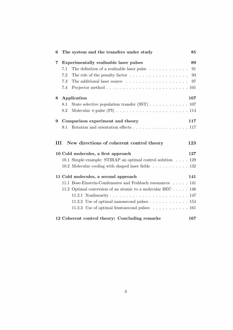
6 The system and the transfers under study 85
7 Experimentally realizable laser pulses 89
7.1 The definition of a realizable laser pulse . . . . . . . . . . . . 91
7.2 The role of the penalty factor . . . . . . . . . . . . . . . . . . 93
7.3 The additional laser source . . . . . . . . . . . . . . . . . . . 97
7.4 Projector method . . . . . . . . . . . . . . . . . . . . . . . . . 101
8 Application 107
8.1 State selective population transfer (SST) . . . . . . . . . . . . 107
8.2 Molecular π-pulse (PI) . . . . . . . . . . . . . . . . . . . . . . 114
9 Comparison experiment and theory 117
9.1 Rotation and orientation effects . . . . . . . . . . . . . . . . . 117
III New directions of coherent control theory 123
10 Cold molecules, a first approach 127
10.1 Simple example: STIRAP an optimal control solution . . . . 129
10.2 Molecular cooling with shaped laser fields . . . . . . . . . . . 132
11 Cold molecules, a second approach 141
11.1 Bose-Einstein-Condensates and Feshbach resonances . . . . . 141
11.2 Optimal conversion of an atomic to a molecular BEC . . . . . 146
11.2.1 Nonlinearity . . . . . . . . . . . . . . . . . . . . . . . . 147
11.2.2 Use of optimal nanosecond pulses . . . . . . . . . . . . 154
11.2.3 Use of optimal femtosecond pulses . . . . . . . . . . . 161
12 Coherent control theory: Concluding remarks 167
ii

Introduction
There has been longstanding interest in optimizing naturally occurring pro-cesses or in controlling them to occur in a specific way. To this end mathe-matician J. Bernoulli developed the formalism of variational calculus, whileengineers build a feedback controlled loop, where the control knobs aresteered according to some signal obtained from the system under control.This approach was so general that it could be applied to any field of naturalscience. In chemistry it was however soon realized, that the control knobsat hand, like temperature, pressure or the choice of a catalyst with whichto influence the outcome of reactions were limited.With the advent of coherent light sources, the continuous wave (cw) lasers,a new possibility of control was realized. The coherence property of lasersallowed to speak of phase as a meaningful quantity, since for the first timeinterference experiments with light were made possible. Then way back inthe 1986 Brumer and Shapiro realized that the concept of interference couldhave potential implications for the control of chemical reactions [1]. As aproof of principle they devised a simple experiment, where initial and finalstate were lower and upper level of an atom. Then they connected bothstates with two light induced pathways, a one- and three-photon transition.A relative phase change between the two lasers of different color allows tochoose between constructive or destructive interference of the two pathwayscontrolling thereby the amount of excited state population. In the same yearTannor, Kosloff and Rice proposed to use coherent pulse sequences beyondthe cw-limit to control the selectivity of reactions [2]. The experimentalrealization of this proposal was however only in reach with the advent offemtosecond laser sources.The rapid development of new laser sources towards ever shorter pulse du-rations spurred the field of coherent control for three main reasons. One issimply related to the pulse duration itself. Control is coherent only if thecoherence or phase relationship in the system generated by the interactionwith the laser pulse survives the control period. Now a number of dephas-ing mechanism that destroy coherence, and distribute the initially localizedenergy all over the system, can occur even on a femtosecond timescale. Thismeans femtosecond laser pulses are really necessary to control these sys-tems. Another argument for short pulse durations is that the controlled
1

2 Introduction
action must match the timescale of the dynamics occurring in the system.The fastest possible motion of nuclei is the vibration of H2 and occurs on afew femtosecond timescale. The 1999 nobel prize in chemistry was awardedto the field of femtosecond pump-probe experiments, since these were thefirst experiments showing snapshots of nuclear motion. Photography of elec-tron motion needs even shorter, attosecond pulses. Another implication offemtosecond pulses is their high intensities and broad spectra hosting a rain-bow of colors. Both of these properties greatly enhance the possibilities ofcontrol since the number of pathways is increased considerably. The manycoherent frequencies make it possible to induce a phase relationship betweentransitions energetically far apart and the high intensities enable highly non-linear processes.But control with light deserves control of the light itself. An ultrashortpulse has a shape, a temporal phase and a polarization state and all of themneed to be controlled and measured accurately. Various methods have beenused to shape femtosecond pulses. Most of these techniques involve devicessuch as liquid-crystal spatial light modulators, acousto-optic modulators, ordeformable mirrors, that are designed to modulate the phase and/or ampli-tude of the dispersed spectral components of a femtosecond pulse [3–6]. Itis routinely possible to generate user-defined waveforms for coherent controlwith these pulse shapers and characterize them using a variety of ultrafastmeasuring techniques. Several experiments show control using simple tai-lored fields [7–13].Unfortunately it is by far not always possible to figure out, how to con-trol a system. The difficulty is to find the optimal tailored pulse, thatleads to the wanted outcome of the experiment by the correct interferenceof the multiple light-induced pathways. Consequently, the optimal controlrevolution began, when Judson and Rabitz proposed to use the feedback orlearning loop, adapted to the experimental techniques used in ultrafast laserpulse control, to solve this search problem [14]. Starting from some initialrandomly tailored pulse a signal, from the system under control, directlycorrelated to the desired aim is used as feedback to a learning algorithm,that accordingly steers the pulse shaper. After thousands of experiments orhundreds of iterations the optimized pulse is automatically found withoutthe need of theoretical input. This idea has been very successfully appliedto many problems in physics, chemistry and biology [15–25].
A similar challenge had to be solved in theory, where the optimal pulseshould drive the theoretical model system in a specified way. Of course themodel system governed by some dynamical equation is devised by the the-orist himself, however this does not imply that the control of the system isalways obvious to him. Therefore, Rabitz [26,27] and independently Tannor,Rice and coworkers [2,28,29] derived a numerical framework named optimalcontrol theory (OCT) using variational calculus. OCT is an iterative pro-

Introduction 3
cedure that solves the control problem by itself. It converges in a few tensof iterations by making use of the known future information and the pos-sibility of backward in time propagation. The fast convergence is essential,since the numerical propagation of the system is very time consuming. Inexperiment this is not an issue, since the quantum mechanical system solvesits dynamical equation in real time. With OCT numerous control problemscould be solved [30–35].
The experimental and theoretical efforts to control quantum systemswith tailored ultrashort pulses constitute the field of coherent control [8,36–40]. The learning-loop in experiment and the OCT in theory are both iter-ative procedures that provide an optimal field in a fully self-contained way.No knowledge about the mechanism is needed as input, but also no under-standing is obtained about the way the field acts to achieve the desired goal.Moreover, no general approach exists to obtain this information. Analyticalcalculations are in this sense more elegant, since an equation is obtaineddescribing the interaction of the tailored field with the system, manifestingthe control possibilities [41–43].
The experimental work in part I of this thesis is part of the first genera-tion coherent control experiments. Simple systems were chosen in order tobe able to derive a closed form equation describing exhaustively the tailoredlaser field interaction with the system. This approach makes the controlmechanism evident. This was a good starting point to test the accurate de-livery of the pulse shape into the interaction region, the limits of the pulseshaping apparatus and the performance of the feedback approach. The newconcept of parameterizations in time and frequency domain was first in-troduced as a method of implementing knowledge into the iterative search,simplifying considerably the interpretation of the control mechanism. Thisallows to establish whether the control is due to, i.e. the ordering of fre-quencies (chirp), some relative phase effect in a pulse train or the numberof interacting pulses. The work on these simple systems has provided basicunderstanding of control mechanisms and later found applications in thecontrol of complex molecular and biological systems.Part II of this thesis tries to adapt OCT in order to bridge the gap betweencoherent control theory and experiment allowing finally for interpretation ofthe optimal result. Modified functionals and strategies are shown that ob-tain simple, robust and realizable tailored laser pulses. Moreover the maskpattern needed to tailor the calculated pulse is defined as direct interfacebetween theory and experiment. This allows to characterize quantitativelyto what extend a laser pulse is reproducible in experiment. Finally it ispossible to check very precisely the correctness of the theoretical model, bynoting discrepancies from theoretically predicted results when applying thecalculated tailored pulse shapes in experiment.

4 Introduction
In part III new applications and concepts of OCT are presented. This workwas done in collaboration with D. Tannor (Weizmann Institute, Israel) andB. Verhaar (TU Eindhoven, Netherlands). Here OCT is applied to molecularcooling with tailored femtosecond pulses and to the partial conversion of anatomic to a diatomic molecular condensate via Raman transition, enhancedby a time-dependent magnetic field sweep over a Feshbach resonance.

Publications
• Thomas Hornung, Marcus Motzkus, and Regina de Vivie-RiedleInfluence of molecular rotation and thermal ensembles on controlJournal of Chemical Physics, in preparation
• Thomas Hornung, Sergei Gordienko, and Regina de Vivie-Riedle andBoudewijn J. VerhaarOptimal conversion of an atomic to a molecular Bose-Einstein-Condensatesubmitted to Physical Review Letters
• Thomas Hornung, Marcus Motzkus, and Regina de Vivie-RiedleTeaching optimal control theory to distill robust pulses even under ex-perimental constraintsPhysical Review A 65, 021403R (2002)
• Thomas Hornung, Marcus Motzkus, and Regina de Vivie-RiedleAdapting optimal control theory and using learning loops to provideexperimentally feasible shaping mask patternsJournal of Chemical Physics 115, 3105 (2001)
• Thomas Hornung, Richard Meier, Regina de Vivie-Riedle, and MarcusMotzkusCoherent control of the molecular four-wave mixing response by phaseand amplitude shaped pulsesChemical Physics 267, 261 (2001)
• Thomas Hornung, Richard Meier, and Marcus MotzkusOptimal Control of molecular states in a learning loop parameteriza-tion in frequency and time domainChemical Physics Letters 326, 445 (2000)
• Thomas Hornung, Richard Meier, Dirk Zeidler, Karl-Ludwig Kompa,Detlev Proch, and Marcus MotzkusOptimal control of one- and two-photon transitions with shaped fem-tosecond pulses and feedbackApplied Physics B 71, 277 (2000)
• Dirk Zeidler, Thomas Hornung, Detlev Proch, and Marcus MotzkusAdaptive compression of tunable pulses from a noncollinear-type OPAto below 16 fs by feedback-controlled pulse shapingApplied Physics B 70, S125 (2000)
5

• Thomas Hornung, Richard Meier, Dirk Zeidler, Karl-Ludwig Kompa,Detlev Proch, and Marcus MotzkusOptimal control of two-photon transitions: bright and dark femtosec-ond pulses designed by a self-learning algorithmUltrafast Phenomena XII, T. Elsaesser, S. Mukamel, M. M. Murnaneand N. F. Scherer eds. (Springer series in chemical physics; 66) p. 24(2000)
• Thomas Hornung, Richard Meier, and Marcus MotzkusFeedback optimization of molecular states using a parameterization infrequency and time domainUltrafast Phenomena XII, T. Elsaesser, S. Mukamel, M. M. Murnaneand N. F. Scherer eds. (Springer series in chemical physics; 66) p. 27(2000)
6

Part I
Coherent controlexperiments
7


Coherent control experiments entered a new era when the ultrafast pulseshaping technology [4,44,45] was developed and Judson and Rabitz proposedthe concept of a learning-loop [14]. They realized that the system to be con-trolled can solve its Hamiltonian in real time and that therefore thousandsof experiments can be carried out in just a second. This is the essential ad-vantage that allows the use of a feedback-loop to solve the inverse problem offinding the pulse that corresponds to a specific solution of the Schrodingerequation without having to resort to theory. The wanted outcome (e.g.bond breaking) is measured by an experimental signal correlated to it (e.g.mass peak of fragment). Differently shaped laser pulses are consecutivelysent onto the system leading to an experimental signal, that again serves asfeedback to measure the performance of each individual laser pulse. This”trial and error“ approach will finally end up with the perfect laser pulse.No knowledge of the Hamiltonian is needed, but the feedback signal mustbe chosen carefully to be really a measure of the desired outcome.When designing a coherent control experiment the following considerationsare of central importance:
1. The wanted outcome must be dependent on the characteristics of thelaser pulse adjustable through the pulse shaping device at hand. Onone hand this implies that the nature of the light used is versatileenough. Especially the hope is that the properties of the laser pulsesin the femtosecond regime their selves (polarization, bandwidth, phase,intensity, ultrafast interaction) are sufficient to the problem (see sec-tion 1.1). Taking again the example of bond-breaking it is essentialthat energy redistribution processes in the system are much slowerthan the local deposition of energy by the laser pulse. On the otherhand the pulse shaping device must have sufficient capabilities to in-dependently change the necessary characteristics of the laser field (seesection 1.1).
2. The ”trial and error“ strategy can be improved considerably if an in-telligent and fast learning scheme is used to adjust the shaping device.This algorithm moreover has to cope with uncorrelated signal changesdue to unavoidable experimental noise (see section 1.2) .
9


Chapter 1
Essentials: The learning-loop
The components of a learning-loop can look very different depending on thespecific application. In abstract terms a learning-loop consists of an actionunder external control which acts on a system and produces there a sys-tem response. Due to the natural correlation between action and responsean algorithm can be used to learn how to change the action to control theresponse in a desired fashion. In the coherent control experiments as al-ready pointed out in the introduction to this chapter the controlled actionare the tailored femtosecond laser pulses. The external control knobs areall integrated in a single pulse shaping device. The system response is thefeedback signal retrieved from experiment. It is feeded into the optimiza-tion algorithm that accordingly steers the pulse shaper to improve the laserpulse shape. The time for the learning-loop to provide an optimal pulse isgiven by the total number of iterations multiplied by the time it takes toperform one iteration. This time is given by the response time of each ofthe elements that constitute a closed-loop experiment: laser repetition rate,pulse shaper, learning algorithm and feedback signal retrieved from experi-ment. Hence it is not possible to be specific, so the total optimization timecan range between a few minutes and several hours. In the following a moredetailed description of a tailored pulse, its characterization and the feedbackalgorithm is discussed. This chapter concludes with a practical applicationof the learning-loop approach: the compression of femtosecond laser pulsesto their bandwidth limit.
11

Initial guess
Learning loop
Pulse shaper
control
probeExperiment
Cell
EvolutionaryAlgorithm
Figure 1.1: A closed-loop process for teaching a laser to control quantum systems.The loop is entered with either an initial design estimate or even a random field insome cases. A current laser control field design is created with a pulse shaper andthen applied to the sample. The action of the control is assessed, and the resultsare fed to a learning algorithm to suggest an improved field design for repeatedexcursions around the loop until the objective is satisfactorily achieved [38].
12

1. Essentials: The learning-loop 13
1.1 Tailored femtosecond pulses
The various techniques to tailor a laser field can be divided into two cat-egories. Those operating directly in the time-domain using fast electronicswitching devices to structure the time-envelope of the pulse and those in thefrequency-domain that shape the spectrum of the pulse. Frequency-domaintechniques are the only suitable for shaping femtosecond laser pulses, sincethese techniques as they operate in parallel on many frequencies of the pulsedo not require electronic switches, which are useless in the femtosecondregime due to their comparatively slow switching times (picoseconds). In-stead spectral shaping is accomplished by a zero dispersion 4-f setup, that isessentially two spectrometers: the first dispersing the spectral componentsonto space in its Fourier plane and the second, used in reversed direction tothe first, collimates again these frequencies to a single beam of light. Thelaser pulse passing this setup does not feel any change, but is essentiallyFourier transformed and back again. Introducing a device (Spatial LightModulator = SLM) that can apply a spatial phase and transmission patternin the Fourier plane of the 4-f setup [see Fig. 1.2] the spectrum of the pulseis modulated [6, 45,46]. The process of shaping can be described by
εout(ω) =M(ω)εin(ω). (1.1)
Here εin(ω) is the spectrum of the incident pulse and εout(ω) of the outgo-
f f f f
grating 1 grating 2
programmable LC mask
Fourier plane
Figure 1.2: Typical setup of a femtosecond pulse shaper, consisting of a SpatialLight Modulator located at the Fourier plane of the 4-f geometry. Here f is thefocal length of the lenses.
ing. The outgoing pulse is the same as the incoming pulse if the 4f-setupis accurately calibrated and the SLM is not addressed externally. Conse-quently, in order for the outgoing pulse to be Fourier limited the pulse mustbe already bandwidth limited as it enters the shaping device. The SLM is

14 1. Essentials: The learning-loop
represented mathematically by a complex function of frequencyM(ω), sincefrequency is mapped onto space according to the dispersion relation of thespectrometer. Eq. (1.1) ignores the effect that the spectral components arealso scattered away from their incoming direction, after passing the spa-tial modulation pattern. This leads irremediably to a shaping of the beamprofile in conjunction with the time structure of the pulse, also known asspace-time coupling [47].SLM’s can be simple static lithographically edged transmission and phasepatterns or more sophisticated programmable devices. Essentially threeSLM types are used in coherent control experiments. An acoustic opticmodulator AOM [5,46], which is a crystal driven by a piezo loud speaker toproduce acoustic waves in it. The ultra fast light pulse sees a snapshot ofthis traveling acoustic pattern and is Bragg scattered acquiring its phasesand amplitudes. Then also adaptive, electrostatically deformable membranemirrors can be used for phase-only shaping [6]. The third type of SLM, aliquid crystal SLM [4] used in this thesis, consists of an array of 128, 97 µmwide active elements (pixels), that change their transmission and/or retar-dance properties according to locally applied voltages. Between each twopixels 3 µm inactive transmitting areas exist, called gaps. The desired mod-ulation pattern is available within the orientation time of the liquid crystalmolecules, which is about 100 ms.The pulse modulated by a LC-SLM along the tilted axis due to the linearspace-time coupling [47] can be expressed mathematically by the discreteFourier transform of Eq. (1.1) [45]
ε(t) =
N/2∑
−N/2
an exp(iφn)εin(t− nτ). (1.2)
The pulse consists therefore of an equidistant comb of subpulses with am-plitudes an and phases φn separated from one another by a finite time τ andextending in time from [−N/2τ,N/2τ ]. This time interval is called effectiveshaping window, since the controllable portion of the modulated pulse canonly extend in this time interval due to a finite number N of adjustable pix-els. The minimal time step τ can be evaluated to be approximately one halfof the incident pulse duration, depending on how much spectrum is madeto fit on the active mask area. In Fig. 1.3 these and further peculiaritiesof the LC-SLM due to its pixelation are depicted and are also describedin Refs. [47, 48]. The spectrum on the gaps is transmitted without beingchanged and therefore recollimates to a weak replication of the incidentpulse at t=0 [Fig. 1.3(b)]. Also replica of the modulated pulse occur outsidethe shaping window inside the antinodes of a sinc modulation pattern in time[Fig 1.3(c)]. This is due to scattering of the frequency components at therectangularly shaped pixels. The finite focal size of the spectral componentshowever smears out this modulation pattern in space leading to a Gaussian

1. Essentials: The learning-loop 15
Figure 1.3: Peculiarities of a liquid crystal Spatial Light Modulator. (a) Desiredpulse shape. (b) Effect of the gaps leading to an unshaped pulse at time zero.(c) Effects due to the discreteness of pixels introducing diffraction of the spectralcomponents and generating pulse replicas. (d) Effect of the finite focal size of eachspectral component leading to a Gaussian weighted suppression of the waveform.
centered around t=0 and diminishing considerably the replica [Fig. 1.3(d)].Due to the space time coupling these replica occur at the outermost parts ofthe spatial profile and can therefore be taken away spatially using a pinhole.The last effect of discreteness to be pointed out is the sampling criterion.As shaping by an LC-SLM can be at best a discrete sampling of a desiredmodulation pattern it suffers from the Nyquist theorem. Nyquist’s samplingtheorem states that a periodic function must be probed at least twice perperiod, or twice over a phase interval of 2π. With reference to a phase func-tion that is to be imposed onto a spectrum, a phase interval of 2π hencemust be sampled by at least two pixels. Consequently the phase jump overone pixel must be much less than π.In order to calculate the mask pattern necessary to tailor a desired pulseshape an algorithm is needed. In the case of phase and amplitude shapinga simple Fourier transform connects the coefficients 128 an and 128 φn val-ues of Eq. (1.1) with the 128 retardance and 128 transmission values of thepixels [47,48]. Things complicate if a pulse form specified by the set (an,φn)is to be produced by phase-only shaping. It is clear that this problem canonly be approximatively solved since 128 phase mask values can not specify256 time domain values characterizing the shape of the pulse. A fast andpractical algorithm to solve this problem is described in Ref. [49].Recent developments of pulse shaping have been to increase the LC-SLMnumber of pixels [50], to modify the setup in order to arbitrarily modulatealso the polarization of the laser pulse [51] and to obtain spatiotemporalcoherent waveforms [52]. Since their exist no liquid crystal materials being

16 1. Essentials: The learning-loop
transmissive and producing the necessary retardance values in the ultravio-let and mid IR, shaping at these frequency ranges was essentially obtainedby frequency conversion of shaped visible pulses [53, 54].
1.2 Feedback algorithm and parameterization
Feedback algorithm. Finding an extremum of a function depending onmany variables is a problem that has been under investigation since theinvention of differential calculus. The primary task of any optimization al-gorithm is to start from an ensemble of suitably chosen initial parametersand then to suggest a revised set which drives the critical observable to-wards the desired optimum, i.e. to generate new search directions in themultidimensional parameter space. Starting from this new parameter set,the procedure is reiterated until some convergence criterion is fulfilled.The algorithm of choice for the learning-loop has to fulfill various additionalproperties: it must be stable against experimental noise, it has to learn asmuch as possible from the feedback signal in order to rapidly improve thetailored pulse performance, it must avoid local maxima and it has to copewith many adjustable parameters namely the voltages applied to the mask.Therefore deterministic schemes such as steepest descent are not suited sincethey are prone to get stuck in local minima and are very sensitive to noise.The learning-loop therefore implements the more suited random schemessuch as evolutionary strategies [55], genetic algorithms [56] and simulatedannealing [57]. Out of these indeterministic schemes evolutionary strategiesare known to be robust against experimental noise [58]. However their con-vergence to a global maximum is not proven mathematically while it is forsimulated annealing.In this thesis an evolutionary strategy which uses 48 individuals (vectors ofLC voltages) was applied. These are randomly chosen and represent onegeneration. For every one of the 48 mask settings of one generation thefitness value is read from the experiment. This serves to quantify the per-formance of each individual. The most successful ones are taken as parentsto the next generation, while the others are discarded. By mutating theparents, i.e. addition of Gaussian white noise with a pre-specified width oneach of the vector elements (genes), and by recombining pairs of parents,i.e. interchanging of their genes, the new generation is built. By successiverepetition of this scheme, only those vectors corresponding to the highestfitness values will survive and produce offsprings (”survival of the fittest“).Mutation serves as dominant search operator, and therefore the extent ofrandom change of each gene must be intelligently restricted. Excessive mu-tation will cause the new search points to be widespread in parameter spaceand no convergence will be achieved. Very small mutational changes, on

1. Essentials: The learning-loop 17
the other hand, will allow only very slow convergence. Hence an adaptivecontrol of the mutation rate [55] was implemented, which ties the amountof change to the number of foregoing mutations which had proven to besuccessful (i.e. produced a better fitness value).
Parameterizations. A very important aspect in optimization is the rightchoice of parameters. A reduction or a specific choice of parameters can leadto an increase in convergence rate, but also to a reduction of the final signalvalue achieved. Instead of using the completely free optimization, where allthe voltages applied to the pixels are taken as individual parameters it can bemuch more efficient to parameterize the mask function or the time envelopeof the pulse. A nonlinear frequency chirp of Nth order would then most effec-tively be parameterized by a polynomial phase function φ(n) =
∑Ni=1 ain
i.Instead of 2 · 128 voltage parameters only N parameters ai would be nec-essary. Similarly a direct time domain parameterization is more suited torepresent, e.g. a train of N pulses with equal amplitude, variable time sep-aration and phase. Here 2N-1 parameters suffice according to Eq. (1.2) tofully characterize such a pulse train. This a much reduced number of pa-rameters compared to a parameterization based on the LC voltage settings.
Parameterization achieves a great improvement beyond the mere reduc-tion of parameters [59,60]. This can best be understood in the abstract no-tion of phase space. One or several optimum solutions for the specific controlprocess are scattered throughout the phase-space of the system considered,hopefully reachable through arbitrary pulse shaping. The algorithm’s taskis to converge into the global optimum after a number of consecutive runs.Since feedback pulse shaping means e.g. trying all different voltages foreach of the 128 pixels of a Spatial Light Modulator (SLM), the number ofparameters can be very high and therefore numerous problems arise, thatone has to cope with: convergence slows down, the possibility to start atdifferent phase space locations to cover different solutions is statistical, im-plementation of theoretical knowledge is difficult and there is no structurein the changes the algorithm performs.Parameterizations establish order into the statistical approach of evolution-ary algorithms and have many important consequences. Each parameteri-zation represents a subset of phase space, meaning phase space is fractionedinto tiny regions of parameterizations. This involves the starting locationson phase space to be predetermined and the algorithm to converge muchfaster since the subset can be chosen to be of a specific size by reducing thenumber of parameters used in that parameterization. This makes it pos-sible to run the algorithm many times and explore thoroughly this chosenregion of phase space for solutions. The importance of incorporating theo-retical information into the experiment is obvious, but the pulses calculated

18 1. Essentials: The learning-loop
by theory are still not always realizable 1) and therefore can only approxi-mately be used as an initial guess. Nevertheless, it is possible to implementthe process, which has been stated by theory to be responsible for the specificcontrol mechanism, into a learning-loop using adequate parameterizations.The evolutionary algorithm then makes only modifications to few parame-ters compatible with the mechanism. Due to these very structured changesone is able to monitor effects induced in the studied system by the prognos-ticated process. The whole pulse shaping phase space is addressed if thereis no parameterization used at all (for the LC-SLM case 2 · 128 independentpixels times ≈ 1000 voltage values). Switching between different parame-terizations in time and frequency domain therefore still allows to cover agreat extent of the pulse shaping phase space with the advantage of havingonly few parameters the algorithm has to operate on. When the algorithmis free to switch between parameterizations it will essentially try out dif-ferent control mechanisms and adapt the most optimal one. This idea isculminated if once a database of control mechanisms is established. Withparameterizations it is moreover possible to perform experiments with moresophisticated feedback signals that take a long time to be retrieved (as anexample see chapter 3).
1.3 Pulse characterization and interpretation
Pulse characterization. Measurement of the optimal tailored pulse is anessential first step in determining the control mechanism. In order to fullycharacterize a femtosecond laser pulse, a measurement technique is neededthat can retrieve the phase φ(t) and intensity I(t) of a laser field, that ismathematically described in the slowly-varying envelope approximation as:√
I(t) exp (iωt+ φ) [61]. The most widely used methods that can even beapplied down to the single cycle 5 fs regime are:
• Frequency resolved optical gating (FROG) [62]. It involves spectrallyresolving the signal beam of an autocorrelation measurement.
• Spectral phase interferometry for direct electric-field reconstruction(SPIDER) [63, 64]. SPIDER is a specific implementation of spectralshearing interferometry. Here an interferometer is used to producetwo pulse replicas that are delayed with respect to one another. Theyare then frequency mixed with a chirped pulse in a nonlinear crystal.Each pulse replica is frequency mixed with a different time slice, of thestretched pulse, and, consequently, the upconverted pulses are spec-trally sheared. The interference between this pair of pulses is recordedwith a spectrometer followed by an integrating detector.
1)The realizability of calculated laser pulses could be considerably improved using strate-
gies presented in chapter 7.

1. Essentials: The learning-loop 19
• Temporal analysis by dispersing a pair of light electric fields (TAD-POLE) [65, 66] is a test-plus-reference spectral interferometer. Anunknown test pulse is mixed at a beamsplitter with a time delayedreference pulse, whose electric field shape is known from a FROG orSPIDER measurement. The pulse pair enters a spectrometer and thetwo spectra combined yield a spectral interferogram. The interfero-gram yields the complete information of the test pulse by a simpleFourier transformation and an inverse filtered Fourier transformation.With TADPOLE it is possible to measure tailored pulses of a few fem-tojoule and also extend the range of measurable pulse complexitiesbeyond the possibilities of the available nonlinear crystals.
The advantage of the interferometric approaches is that they requireonly a one dimensional data set to reconstruct the one dimensional field andcan use a direct data inversion to do so in real time. In contrast the FROGtechnique measures a two-dimensional representation of the one-dimensionalfield and consequently requires the collection of a relatively large amount ofdata. The needed algorithm to invert the data and reconstruct the field isthereby more sophisticated. The advantage of FROG is of practical natureas it does not require a new apparatus since mostly an autocorrelator andspectrometer are available.In this thesis the second-harmonic FROG (SHG FROG) technique was usedto characterize the tailored pulses. A more detailed description of this tech-nique follows. The method measures the spectrogram of the pulse, which issufficient to completely determine ε(t) [62] (besides the absolute phase)
S(ω, τ) =
∣∣∣∣∣∣
∞∫
−∞
dt ε(t)g(t− τ) exp(−iωt)
∣∣∣∣∣∣
2
. (1.3)
Here g(t− τ) is the gate function used to represent the autocorrelator typeused. The autocorrelator using second harmonic generation has a gateg(t, τ) = ε(t)ε(t − τ). Measuring the spectrogram hence means to acquirethe spectrum of the autocorrelation signal for each time delay τ . The al-gorithm used to retrieve the complete pulse shape from this spectrogramis based on the method of generalized projections. It is quite sophisticatedand will therefore not be explained. The interested reader should refer toRef. [62]. It should be noted however that in the case the incident laser fieldto the pulse shaping device is well characterized it is possible to use the pulseshaping equation to make a rough ”measurement“ of the outgoing tailoredpulse. The mask pattern itself then serves to characterize the shaped laserfield, of course under the premise that further material in the optical pathafter the pulse shaper does not have a measurable effect on the pulse shapeor can be accounted for.

20 1. Essentials: The learning-loop
Interpretation. The result of an optimization run is the maximumyield achieved and the respective mask pattern and optimized laser field.The laser field shows usually such a complex shape, that it is completelyobscure what essentially the control mechanism is. In order to answer thisquestion several approaches can be pursuit. Purely experimental approachesinclude the following possibilities: The learning-loop iteration can be re-peated several times with different initial guess laser pulses generations. Theoptimal mask patterns attained can be then compared to find similarities.Perhaps groups of similar mask patterns then identify the control pathways.Another approach used is to shoot the laser pulse not only onto the exper-iment of interest but simultaneously on a second experiment with a wellknown response. This reference experiment could be for example a non-resonant two-photon transition in an atom. If the experimental signal cor-relates closely with the reference than the control mechanism is clearly thesame, i.e. a non-resonant two-photon transition [67].A very powerful technique was already discussed earlier and is the conceptof parameterization. Here, changes applied to individual pulse parameterscan determine whether the control is due to the specific pulse separation,chirp or phase relationship.Perhaps the best way to obtain the control mechanism is to compare theobtained laser pulse with optimal control theory predictions. However inorder to do so there is a gap to surmount between them as will be discussedin detail in part II of this thesis [60, 68].
1.4 Simple example of a learning loop application:pulse compression
In this section a simple learning-loop setup is realized with the aim of com-pressing femtosecond pulses originating from an optical parametric amplifierwith noncollinear-type phase-matching [69–73]. This simple, but technicallyimportant example shall illustrate the individual elements, that constitutea learning-loop as discussed previously and acts as easy introduction to theautomated control experiments of increasing complexity in the next chap-ters.Pulse compression is commonly achieved by phase-only shaping. The centraltask is to apply on the shaper the exact phase function compensating for theintrinsic phase of the pulse, that leads to pulse lengthening and distortion.Especially ultrashort pulses in 20 fs regime as considered here, suffer fromgroup velocity dispersion (GVD) of second and higher orders introduced bydispersive elements installed in the beam path behind the compressor, suchas cell windows, wave plates, cuvettes filled with solvents, etc. A majorproblem is hence the faithful delivery of ultrashort pulses to the locationwhere the actual experiment is performed, especially when the ultrafast dy-

1. Essentials: The learning-loop 21
namics of molecules in liquid solvents is to be investigated.An elegant solution to this problem is presented here, where phase tailoringof 20 fs ultrashort pulses steered by an evolutionary algorithm is used tocompress distorted pulses to their bandwidth limit at any chosen point inthe experiment [74–76]. The main advantages of the setup are the swiftnessof the automated compression procedure (typically less than five minutes)and the capability to compensate phase distortions of arbitrary appearance.The learning-loop setup was optimized to the problem at hand by build-ing a pulse shaper able to support the broad bandwidth of the pulses, bychoosing an adequate parameterization and finally by choosing a feedbacksignal reaching a maximum for a flat phase or shortest pulse duration. Aschematic of the learning-loop setup is shown in Fig. 1.4.
PMT
BBO (10µm)
filter
optimization
algorithm
f=200mm
ACnc-OPA
LC
Figure 1.4: Learning loop setup for automated compression of pulses from anoncollinear OPA [76].
Pulse shaper. An essential requirement for high-quality shaping is anaccurate Fourier transformation from the time into the frequency domainand back. The pulses must pass the shaping unit undisturbed as long as nofiltering is performed. This is especially restrictive for femtosecond pulsesbelow 30 fs. Great care must thus be taken to avoid clipping of the spec-trum (80 nm full width at half maximum) at the aperture of the LC mask.The overall accepted bandwidth of this shaper was designed to be abovethat of the pulses generated by the noncollinear OPA. Imaging distortion bychromatic aberration becomes important for these very broad spectra andmust be avoided. Therefore an all reflective pulse shaping setup is desired,where the lenses are replaced by mirrors [77]. Cylindrical optics are used toreduce the power density impinging on the LC mask and thus prevent dam-age. The off-axis angles are kept as small as possible to alleviate imagingaberrations introduced by the focusing mirrors. To ensure that the shaperacts as a zero-dispersion compressor as long as the LC mask is inactive, a

22 1. Essentials: The learning-loop
pair of prisms before the shaper was installed in a first run to compress theincident pulses close to the Fourier limit (< 20 fs). The shaper was thenadjusted until the outgoing pulse was not further broadened.
Feedback signal. The frequency doubled light captured by a photomul-tiplier tube (PMT) after focusing the tailored pulse with a spherical mirror(f = 200 mm) onto a nonlinear crystal (BBO, 10 µm), serves as feedbacksignal. A spectral filter (UG-11) in front of the PMT blocks the fundamentalwavelengths. This feedback signal is proper since bandwidth limited pulsesgenerate maximum SHG signal [75].
Parameterization. Since GVD leads to smooth reshaping of the pulsephase, the most efficient parameterization is of polynomial type
Φn =
Kmax∑
k=2
ck
(n−N0
N
)k
, n = 0, . . . , N − 1 = 127, (1.4)
with quadratic terms (k = 2) as lowest polynomial order k since constant(k = 0) or linear (k = 1) phase terms only produce a phase- or time- shift,respectively. In all the following compression experiments the optimizationprocedure was confined to the search for only second and cubic order phases,i.e. Kmax = 3 in Eq. (1.4). The parameters ck and N0 are optimized bythe algorithm. Because the spectrum of the OPA is widely tunable, N0 hasbeen included as parameter to ensure that the offset of the phase functioncoincides with the center of the spectrum after the optimization has beenaccomplished. Alternative concepts of parameterization such as linear ap-proximation or cubic splines were tested as well but resulted in many moreloops of the algorithm while eventually achieving comparable pulse dura-tions.Having setup the learning-loop its performance is ready to be tested. Thechirped output pulses of the noncollinear OPA with a pulse duration of 270fs [see Fig. 1.5(c)] were sent into the pulse shaper without previous compres-sion using a prism compressor. The algorithm was then applied and a pulseduration below 16 fs was again obtained [see Fig. 1.5(a) and 1.5(c)]. The au-tocorrelation measurements were performed in a noncollinear arrangement,either with a 10-µm BBO crystal, or with a 2-photon SiC diode [78]. Themask pattern found by the algorithm to compress the output pulses to theirFourier limit had mainly quadratic chirp [Fig. 1.5(b)]. Since the phases arespecified to within modulo 2π wrapping of the phase occurs if the 2π inter-val is exceeded. Unwrapping of the phase mask pattern in Fig. 1.5(b) wouldreveal a strongly curved parabola over all the mask pixel area.The convergence data of Fig. 1.6 shows the feedback value of the best andworst individual of each generation. In addition the mean feedback value ofbest and worst is calculated for each generation. At the beginning a random

1. Essentials: The learning-loop 23
Figure 1.5: (a) Autocorrelation of the pulse behind the shaper after polynomialphase optimization. (b) Optimal phase function applied on the mask by the algo-rithm. (c) Compressed (hollow dots) and uncompressed (filled dots) pulse.
generation is created, whose performance can be already significant depend-ing on the number of individuals and the complexity of the optimizationproblem. The evolutionary selection then leads to an increase of the bestfeedback value over the number of iterations until it stagnates at its opti-mum value. The fluctuation of this value depends on experimental noiseand also on the sensitivity of the control parameters - that is large jumpsare expected if small changes to the control parameters have a large effecton the feedback signal. This is clearly visible in Fig. 1.6. On the contrary,if the noise level is low and insensitive parameters are used a smooth in-crease and also an approach of worst and best feedback signal indicatingconvergence would be expected. The terminal value of the SHG signal wasapproached after about 25 generations. At a pulse repetition rate of 1 kHzand averaging over 50 pulses the adaptive compressor thus compensates thechirp and produces short output pulses in less than five minutes. This figureshould be still reducible with a biased initial population taking advantageof a-priori physical knowledge such as the supposed sign of the chirp to becompensated. With other parameterizations of the phase function, it wasfound that the convergence speed as well as the final SHG value was de-pendent on the internal strategy parameters of the algorithms. As a rule ofthumb: the more complex the optimization, for example the more parame-

24 1. Essentials: The learning-loop
Figure 1.6: The convergence curve of pulse compression as measured by theintensity of the SHG signal. Fitness of best (filled dots) and worst (hollow dots)individual of each generation. A mean is also calculated (line).
ters to optimize, the more “careful” the optimum has to be approached bya proper choice of internal strategy parameters mentioned above. This hasbeen investigated in detail in Ref. [58].

Chapter 2
Control of atomic transitionswith phase-related pulses
The following experiment is part of the first generation of coherent controlexperiments. At this time it was essential to characterize the effectivenessof the learning-loop and find an answer to the following questions:
• Did the algorithm converge to the global maximum? Is the resultdependent on the initial guess?
• How many iterations are necessary? How long does an optimizationrun take?
• When do the optimal pulses coincide with theory? How can the as-sumptions of theory be met?
• Is the pulse shape seen by the atoms or molecules in the interactionregion really the one applied and measured a distance away? Or is itdistorted by pulse propagation, absorption or focusing?
• What is the importance of an accurate initial guess?
The control of the one and two-photon-transition in the sodium atom waschosen due to the existence of an accurate theory predicting already thecharacter of the optimal solutions. This close link between theory and exper-iment allowed to quantify the above answers and use the atom to ”calculate“solutions beyond the analytical limit.
2.1 Experimental setup
The femtosecond pulse source for experiments on sodium was a commercialTi:Sapphire laser system (CPA-1000, Clark MXR Inc.) which supplied 1 mJ
25

26 2. Control of atomic transitions with phase-related pulses
/ 100 fs / 800 nm pulses at a repetition rate of 1 kHz. Frequency conversionto the wavelength interval between 580 nm and 700 nm in an optical para-metric amplifier (IR-OPA, Clark) yielded pulse energies around 5 mJ. Theprogrammable pulse shaping apparatus is a symmetric 4-f arrangement [4]composed of one pair each of reflective gratings (1800 lines/mm) and cylin-drical lenses (f = 150 mm). Its active element - a liquid crystal (LC) mask -is installed in the common focal plane of both lenses. Meticulous alignmentmust ensure zero net temporal dispersion. This is achieved once the shapesof input and output pulses match as long as the LC mask is turned off. Thetechnique of frequency resolved optical gating (FROG) [62] served to charac-terize the generated pulses. Sodium was evaporated in a heat pipe oven [79]pressurized with 10 mbar of Argon as a buffer gas. The temperature wasset sufficiently low (520 K) to eliminate pulse propagation effects [80, 81].The experimental setup is sketched for the one- and two-photon control inFig. 2.1. Details of the excitation and detection schemes will be supplied incontext with the respective experiments.

controlleroptimizationalgorithm
pulse shaper
pulse shaper
controller
PMT
OPA100 fs
Dye laser
2ns
heat pipe
G(a)
(b)
excitation scheme
5s
3s
4p
3p3/2
3p1/2
3s
τ
OPA100 fs
PMT
F
heat pipe
feedback 4p
λ
monitor 3p
PMT
Figure 2.1: Experimental setup. (a) Collinear pump-probe arrangement to controlthe one-photon excitation of Na via a double-pulse sequence. The inset illustratesthe pertinent spectroscopic details. τ marks the delay between both pulses. (b)Experimental layout and spectroscopic details of the pump- and detection schemesof the two-photon experiment. Fluorescence from 4p serves as feedback to thecontrol algorithm.
27

28 2. Control of atomic transitions with phase-related pulses
2.2 One-photon Na(3s → 3p) transition
In pursuit of the goal to control the one-photon transition in sodium [seeFig. 2.1(a)] we employed phase- and amplitude shaping of the incident spec-trum centered around 589 nm to generate a phase-related double-pulse se-quence [see Fig. 2.2]. Moderate focusing (f = 300 mm) into the heat pipe
Figure 2.2: Typical FROG calculation, in the time domain, of pulse envelope (a)and phase of a generated double pulse (b).
resulted in a power density of ≈ 1011 W/cm2 which was sufficient to saturatethe 3s → 3p transfer. Only the population induced in the 3p1/2 state wasprobed with a narrowband (∆ω = 0.2 cm−1) Nd-YAG pumped dye laser(20 µJ, 3 ns, 50 Hz) which was fired synchronous with the Ti:Sa system andtuned to the 3p1/2 → 5s [see Fig. 2.3]. Pump and probe beams were alignedcollinearly and diligent care was taken to ensure that the probed volumewas completely overlapped by the pump.In the following we will give a theoretical description of the response of
this two-level system to the sequence of two phase-related pump pulses. Thetreatment will be restricted to the 3s (|1〉) and 3p1/2 (|2〉) states and thetemporal evolution of the excited level as induced by the pulse pair. Co-herences between the finesplit 3p levels due to broadband excitation are notdetected as only 3p1/2 is probed. The phase of the initially excited popula-tion evolves freely in time as exp(iω12t) and later interferes with the differentphase of the population induced by the follow-up pulse. The description ofa one-photon absorption in a first order approximation yields a populationof the probed excited state which is given by |c2(t)|2 , where
c2(t) =2π
i~
t∫
−∞
dt Hs12(t
′) exp(iω12t′) (2.1)

2. Control of atomic transitions with phase-related pulses 29
5s
3s
3p1/2δω
ω0
3p3/2
ω12
τ
Figure 2.3: Level scheme of the sodium atom, showing the one photon transitionfrom 3s to 3p1/2 and 3p3/2. Due to the broad bandwidth of the laser pulse both 3plevels are coherently populated. In the experiments only the 3p1/2 level populationis probed by a nanosecond laser tuned in resonance to 5s. The frequency between3s and 3p1/2 is denoted ω12 and the femtosecond laser with center frequency ω0
is detuned by δω from the probed 3p1/2 level. The two arrows separated by τindicate, that the excitation is performed with a tailored double pulse having avariable interpulse separation τ .
Hs12(t
′) is the interaction Hamiltonian which, assuming the dipole approx-imation, is given by Hs
12(t′) = µε(t′), where µ is the dipole moment and
ε(t′) symbolizes the electric field of the laser pulse. In the slowly varyingenvelope limit a pulse is described as a time dependent envelope functionincluding a carrier wave with the central frequency of the laser field, ω0.This approximation is valid for pulse durations down to a few femtoseconds.
A phase-related double pulse can be created in two ways, simply by a in-terferometer or alternately using arbitrary pulse shaping and will be used inthe following to control the population in the excited state of the one-photontransition. To later understand the two control limits a clear definition ofthe phase of a femtosecond pulse will be given here. A femtosecond pulsehas a constant zero phase if the maxima of electric field and envelope coin-cide. When the electric field is displaced with respect to the envelope thepulse has a constant nonzero phase in time. The delay between two pulses isdefined as the difference in time between the maxima of the pulse envelopesirrespective of the phase, that each individual pulse has. This definitionapplies to what happens in the time domain.However as is clear from section 1.1 pulse shaping is best expressed in thefrequency domain, since this naturally takes into account that the spectrum

30 2. Control of atomic transitions with phase-related pulses
of the pulse can not be increased by additional frequencies. Therefore thebest comparison between an optical delay line and the pulse shaper capabil-ities can be seen in the frequency domain [82].In this domain, as can be seen easily by calculating the Fourier transform,the phase of a pulse is given by the intercept of the φ(ω) at ω = 0 and thedelay between the pulses is simply given by the slope of the phase functionat ω0
1). An interferometer with an ideal delay line in one of its arms isonly able to create a pulse pair with the same phase as shown in Fig. 2.4.This can be calculated by using the Maxwell equations and the field is givenmathematically by the following equation [see also Fig. 2.4(a)].
ε(t) =2∑
n=1
exp
[
−(t− nτ∆
)2]
cos[ω0(t− nτ)] (2.2)
Note that both pulses do not share a common carrier wave2), but insteadboth have a constant temporal zero phase irrespective of their pulse sepa-ration. In the frequency domain this translates to the spectral phase shownfor different delays in Fig. 2.4(b). As the delay is increased the slope of thephase function of the second pulse increases, while the intercept is alwayszero showing that both pulses are phase locked.The possibilities to create a phase-related double pulse are maximal whenusing a pulse shaper. The phase and delay can be changed independentlyfrom one another. Exemplarily in Fig. 2.5 a double-pulse is shown thatshares a common carrier wave. That is the envelope slides over this commoncarrier as the delay is changed. The carrier is shown as dotted line. Hencethe phase of the second pulse must change as -ω0τ if τ is the delay. Thiscan be most intuitively seen again in the frequency domain [see Fig. 2.5(b)].The intercept at ω = 0 changes exactly according to φ(ω) = −ω0τ as thedelay is changed, while the phase at ω0 stays always zero showing that bothpulses share a common carrier wave. This is mathematically expressed bythe following equation [see also Fig. 2.5]
ε(t) =2∑
n=1
exp
[
−(t− nτ∆
)2]
cos(ω0t) (2.3)
Of course a pulse shaper can be used to generate double pulses which areany intermediate configuration between the case discussed here and the idealinterferometer case of Fig. 2.4. Since the one-photon transition is sensitiveto the relative phase of the double pulse, the control parameter, the twomethods can be distinguished. In order to see this the equations for the in-terferometer case are derived and thereafter the pulse shaping case is studied.
1)Not considered here are orders of the phase function higher than one, since these are
not needed to create phase-related double pulses.2)A carrier wave is defined by its frequency and the phase

(a) (b)
0ω0
ω
φ(ω)
Figure 2.4: Double pulse created by a Mach-Zehnder interferometer (ideal delayline). (a) Electric field of both pulses have the same phase, i.e. they are phaselocked. They have no common carrier wave and are given by the equation in (a).(b) Spectral phase of the second pulse in (a). Note that the intercept a ω = 0 is 0,showing that both pulses are phase locked. Increasing phase slopes correspond toincreasing pulse separations.
(a) (b)
0ω0
ω
φ(ω)
Figure 2.5: Double pulse as can be created using a pulse shaper. (a) Envelopeof both pulses slide over a common carrier wave, i.e. the two electric fields havedifferent phases. Mathematically they are expressed by equation in (a). (b) Spectralphase of the second pulse in (a). Note that the intercept a ω = 0 is given by -ω0τ ,while the phase is zero at ω0 showing that both pulses have common carrier wave.Increasing phase slopes correspond to increasing pulse separations.
31

32 2. Control of atomic transitions with phase-related pulses
Interferometer. Splitting a pulse creates two pulses with the samephase. The time separations between the pulses can be adjusted with adelay stage [see Fig. 2.4]. The electric field is then
ε(t) = exp(−iω0(t− t1)) exp(iφ1)a1(t− t1)+ exp(−iω0(t− t2))a2(t− t2) exp(iφ2) (2.4)
Setting t1 = 0 and φ1 = 0 and introducing the time separation t2 = τ andphase relationship φ2 = δφ the equations simplifies to
ε(t) = exp(−iω0t)a1(t) + exp(−iω0(t− τ))a2(t− τ) exp(iδφ). (2.5)
Inserting this expression into Eq. (2.1) one obtains
c2(t) ∝t∫
−∞
dt′ exp(iδωt′)a1(t′) +
[ t∫
−∞
dt′ exp(iω12(t′ − τ)) exp(iω12τ)
exp(−iω0(t′ − τ))a2(t
′ − τ) exp(iδφ)]
c2(t) ∝ f1 + f2 exp(iω12τ) exp(iδφ)
|c2|2 ∝ cos(ω12τ + δφ) (2.6)
In ideal interferometers δφ = 0 3), hence the phase can not be influenced andchanging τ will lead to a signal from the excited state that is periodic with afrequency of the one-photon transition frequency ω12. For the sodium atomthis frequency is ω12 = 2π/1.97 fs and will induce very fast oscillations ofthe probed signal. This signal is not resolvable using the LC based pulseshaper to adjust the interpulse separation, since the minimal time step isrestricted due to pixelation to about 40 fs (see section 1.1). Such atomicoscillations were investigated earlier in Cs by Blanchet et al. using a stabi-lized interferometer [12].
Pulse shaping. In frequency domain pulse shaping the phase differenceδφ of the double pulse pair can be chosen arbitrarily and independent of itsseparation in time, τ . Contrary to the interferometer case if only the pulseseparation τ in a shaped double pulse is changed the phase will changeaccording to δφ = −ω0τ , since the pulses slide over a common carrier wave[see Fig. 2.5]. Pulse shaping however allows to apply an additional phase α,so that δφ = −ω0τ+α and complete control over the pulse phase is recoveredirrespective of τ . Inserting this relation for δφ into Eq. (2.6) results in [83,84]
|c2|2 ∝ cos(ω12τ − ω0τ + α)
|c2|2 ∝ cos(δωτ + α), (2.7)
3)In reality the mirrors in the delay stage if not interferometrically stabilized will make
the phase relation fluctuate around this mean value of zero.

2. Control of atomic transitions with phase-related pulses 33
where δω = ω12 − ω0 stands for the detuning of the laser frequency fromthe one-photon transition, here 3s → 3p1/2. This equation predicts, that achange of the temporal pulse pair spacing while α = const. induces a slowoscillation characterized by the detuning. Note that the physical phase ofthe second pulse, that is the position with relation to the carrier is given byφ2 = −ω0τ +α in Eq. (2.7). Again we note here the important difference tothe interferometer case: applying mask patterns that change τ at constantα, will in reality change the phase of the second pulse, since the envelope isdisplaced over the carrier wave. This can be seen in the following sequenceof plots [see Fig. 2.6], resembling a set of tailored double pulses with differingtime separations, but constant α = π. The column (a) shows the electric
-π
π
0
0
1
-π
π
0
-π
π
0
0
1
-π
π
0
-π
π
0
0
1
-π
π
0
-π
π
0
0
1
-π
π
0
time time-π
π
0
pixel0
1
pixel-π
π
0
(a) e(t) (b) φ(t) (c) |M(ω)| (d) φ(ω)
Figure 2.6: Shaping a sequence of double pulses with α = 0 differing only in theirtime separation τ . Since both pulses have a common carrier wave, their relativephase changes as ω0τ , where ω0 is the center frequency of the laser. (a) column:Electric fields. (b) column: Phase in time. (c) column: Transmission mask patterns.(d) column: Phase mask patterns.
fields, (b) the flat phase of the pulses in time, (c) and (d) the correspondingtransmission and phase pattern on the SLM. The wiggling (or better theslope if unfolded) of the mask patterns increases as the pulse separationbecomes bigger. The intercept (not shown) as known from the previousdiscussion changes here as -ω0τ .
34 2. Control of atomic transitions with phase-related pulses
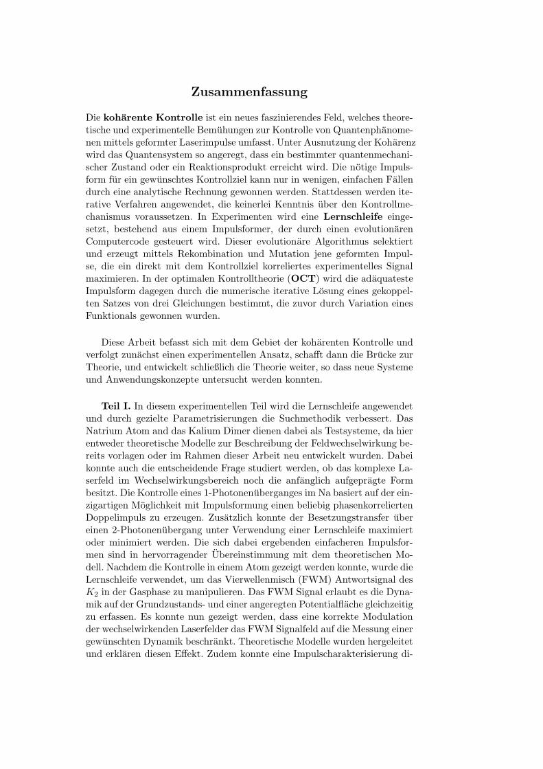
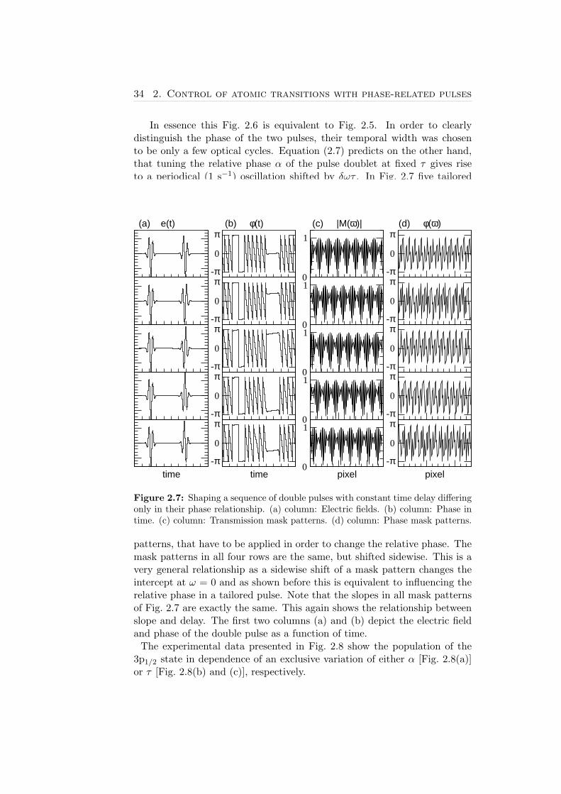
In essence this Fig. 2.6 is equivalent to Fig. 2.5. In order to clearlydistinguish the phase of the two pulses, their temporal width was chosento be only a few optical cycles. Equation (2.7) predicts on the other hand,that tuning the relative phase α of the pulse doublet at fixed τ gives riseto a periodical (1 s−1) oscillation shifted by δωτ . In Fig. 2.7 five tailoreddouble pulse pairs at constant separation τ are shown, where merely thephase parameter α was changed. The (c) and (d) column show the mask
-π
π
0
0
1
-π
π
0
-π
π
0
0
1
-π
π
0
-π
π
0
0
1
-π
π
0
-π
π
0
0
1
-π
π
0
time time-π
π
0
pixel0
1
pixel-π
π
0
(a) e(t) (b) φ(t) (c) |M(ω)| (d) φ(ω)
Figure 2.7: Shaping a sequence of double pulses with constant time delay differingonly in their phase relationship. (a) column: Electric fields. (b) column: Phase intime. (c) column: Transmission mask patterns. (d) column: Phase mask patterns.
patterns, that have to be applied in order to change the relative phase. Themask patterns in all four rows are the same, but shifted sidewise. This is avery general relationship as a sidewise shift of a mask pattern changes theintercept at ω = 0 and as shown before this is equivalent to influencing therelative phase in a tailored pulse. Note that the slopes in all mask patternsof Fig. 2.7 are exactly the same. This again shows the relationship betweenslope and delay. The first two columns (a) and (b) depict the electric fieldand phase of the double pulse as a function of time.The experimental data presented in Fig. 2.8 show the population of the
3p1/2 state in dependence of an exclusive variation of either α [Fig. 2.8(a)]or τ [Fig. 2.8(b) and (c)], respectively.

Figure 2.8: Population of Na (3p1/2) vs. characteristics of double pulse. (a)α-transient. The relative phase α is varied and plotted for three different pulseseparations τ (1.2, 1.6, and 2.0 ps). Cosine functions are fitted to the data. Theslope of the lines connecting the maxima allows to deduce the detuning δω. (b)and (c) τ -transient. The pulses are set to equal phase α while the time separationτ is changed. The time step resolution is 1×40 fs for (b) and 2×40 fs for (c).
35

36 2. Control of atomic transitions with phase-related pulses
This kind of shaping was obtained by applying the mask patterns ofFig. 2.7 or Fig. 2.6, respectively. The detuning δω can be calculated fromthe slope of the lines connecting the maxima of the cosine modulation. It isδω ≈ π
c·800fs=131cm−1. While Fig. 2.8 (a) agrees perfectly with the pulseshaping model [see Eq. (2.7) and Ref. [4]], a change of the pulse spacingseems to cause an ambiguous picture. An oscillatory behavior of the popu-lation which exceeds the capability of time resolution of the pulse shapingsetup is superimposed by a slow modulation approximately proportional tothe detuning [see Fig. 2.8(b) and (c)]. This is in distinct contrast to theexpected slow oscillation. If the phase of the second pulse would obey ω0τas a function of the time difference τ , as is presumed when pulse shaping isperformed, only a slow oscillation should show up. This can be explainedalso in a simple physical picture. The phase of the population excited by thefirst pulse into the 3p1/2 state begins to evolve in time as −ω12t. The phaseof the follow-up pulse as it slides over the carrier evolves with the carrierfrequency and is −ω0t. In the case the laser center frequency would be inperfect resonance with the one-photon transition a phase locking betweenthe laser field and the atom would be achieved, since both phases wouldbe the same at all times evolving in absolute harmony with each other. Inthis case the follow-up pulse excites a second population that will alwaysconstructively interfere with the population already in the 3p1/2 state andno modulation would be visible; δω = 0 and Eq. 2.7 reduces simply to|c2|2 ∝ cos(α). For any slightly off-resonant excitation one then simply ex-pects a slow modulation, since the phase evolution of the first excited 3p1/2
state population is only partly compensated for by the carrier phase evolu-tion. The worst case being the interferometer case, where the phase of thesecond pulse does not change as a function of the pulse separation and themaximum phase dynamics of the probed 3p1/2 state is then visible in theτ−transient. Stated in other words, the τ−transient is simply the phaseevolution of the excited state population that an observer sees when he islocked to the phase of the follow-up pulse. In the case of pulse shaping thephase of the second pulse is locked to the carrier frequency and therefore theobserver sees effectively a rotating wave approximation of the excited statephase dynamics.Referring again to the experimental data, where a very fast not resolvableoscillation is observed, the conclusion is that the shaper cannot create doublepulses sharing a common carrier wave, as would be expected for constantα. As it seems, the phase of the second pulse does not accurately obeyφ2 = −ω0τ as a function of the delay with respect to the first. The exper-imental transient reveals a beating pattern which is seemingly expressibleas the sum of cosines with frequencies δω, ω12, ω0. Such a transient wouldindeed appear if, next to the two pulses with variable time separation τ shar-ing a common carrier wave [ideal pulse shaper, Eq. (2.7)], a third pulse witha fixed phase would act on the system. This third pulse could be created

2. Control of atomic transitions with phase-related pulses 37
by reflection on beam optics or as in a detailed discussion by Wefers andNelson [47] have shown that the passively transmitting gaps of the liquidcrystal array give rise to such an additional pulse. Notwithstanding its lowintensity it must be considered in the regime of saturation where this ex-periment was performed. Both possibilities would describe this third pulsewith Eq. (2.6). Another tentative explanation of the τ -transient rests on theassumption of a general nonlinear τ -dependence of the phase of the secondpulse. This would ascribe the displacement of the phase from its ideal linearω0τ behavior of the second pulse to inhomogeneities in the shaper.In conclusion, measurements which show the feedback of the controlled one-photon excitation to a variation of τ represent an extremely sensitive cri-terion of the quality of a pulse shaper incorporating a discrete mask andcould serve to quantify the deviation from ideality, since an “ideal” shapersatisfies the condition formulated in Eq. (2.7). A possibility is to record theτ -transient with enhanced temporal resolution by using shorter pulses, byincreasing the number of pixels, and by performing an analogous experimentaddressing an atomic transition in the IR (smaller ω12). This should pro-vide deeper understanding of the physical reasons which are behind thesesurprising results.
2.3 Two-photon Na(3s →→ 5s) transition
The objective of the study that will be presented in the forthcoming chap-ter is the coherent control through spectral phase manipulation of a nonresonant two-photon process via feedback optimization steered by an evo-lutionary algorithm. The aim is to find tailored pulses that maximize orminimize the two-photon transfer of population 3s →→ 5s in sodium. Dueto the broad bandwidth of the laser pulse multiple pathways connect initial3s and final 5s state. Therefore controlling the relative phase of each tran-sition will lead either to constructive or destructive interference, “bright”or “dark” tailored pulses. A schematic diagram of the experimental layoutas well as the relevant spectroscopic details of the employed pump and de-tection scheme are displayed in Fig. 2.1(b). The exciting laser was tunedto λ = 598 nm which is close to the 3s →→ 5s resonance, and focused toprovide a maximum power density of ≈ 1011 W/cm2 inside the heat pipe.The population of the 5s target level optically decays to 3p or undergoes col-lisional relaxation to the 4p state [see Fig. 2.9]. Both levels are monitoredseparately via their fluorescence to the 3s ground state at 589 nm and 330nm, respectively. Due to the spectral width of the ultrashort 598 nm pulsesa competitive (1+1)-photon excitation of 5s via 3p (at 589 nm) can not beexcluded right away. The low frequency wing of the spectrum is in resonancewith this strong one-photon 3s→ 3p transition. It must be thus offered evi-dence that the 5s level is indeed populated as the result of only non resonant

38 2. Control of atomic transitions with phase-related pulses
5s
3s
4p
3p
Ω ω0
Figure 2.9: Level scheme of the sodium atom, showing the two photon transitionbetween 3s and 5s. Due to the broad bandwidth of the laser pulse several two-photon transition pathways exist. The 3p levels are excited by the wings of thespectrum and leads to 1+1 resonant enhancement. The frequency between 3s and5s is denoted by ω0. The detuning from half of this frequency (ω0/2) is given byΩ. The 5s population decays to the 3p levels and also via 4p back to 3s.
two-photon pathways; only then experiment can be directly compared withthe theory of Ref. [11] that will be presented later. To show that indeedspectral blocking of the low frequency wing of the spectrum suppresses the1+1 photon transition via 3p a prediction from a theoretical treatment ofthe quantum control of multiphoton transitions by shaped ultrashort pulseswhich excludes strong field effects by Meshulach et al. [41] will be exploited.In this paper they calculated the effect of a mask pattern consisting of πphase step on the probability of N-photon absorption in a two-level system.The plots of this quantity vs. the normalized step position peak at the fre-quency of the N-photon absorption. They are symmetric with respect to thismaximum and vanish for N values of the phase step position. The numberof minima is thus indicative of the order of the absorption process. Fig. 2.10shows the experimental result for the 3s →→ 5s transition as a function ofthe π step position induced by the SLM. The position of the maximum andthe occurrence of two symmetrically arranged minima suggest a two-photonprocess induced by a wavelength of ≈ 602 nm. This number is directlyread from a spectrum of the laser pulse which was taken while pixel #43(maximum) was blocked (see Fig. 2.10). The implementation of a feedbackcontrolled optimization routine requires to identify an observable which isuniquely tied to the quantity to be controlled. Population of 5s gives rise tofluorescence from the 3p and 4p levels. 3p may, however, also be pumpedin a 589 nm one-photon step from 3s. The text to follow describes twoexperiments which address and settle this tentativeness. The data of thefirst test are illustrated in Fig. 2.11 and show the fluorescence from the 3p

2. Control of atomic transitions with phase-related pulses 39
Figure 2.10: (a) π phase step shifted across the mask. Fluorescence from collision-ally populated 4p shows symmetry around pixel #43. (b) OPA spectrum behindSLM observed with pixel #43 set to minimum transmission and left spectral wingblocked by a razor blade.
and 4p levels, following excitation of 5s by 1 mW of unchanged or modifiedpump pulses. The latter were obtained by clipping, in the Fourier plane,the blue wings (<591 nm) of the frequency spectrum. The ensuing pulsespectrum is shown in the right panel of Fig. 2.10. Fluorescence from 4pappears with equal intensity for either excitation condition. The 3p analog,however, is drastically diminished in the absence of the wavelength match-ing the one-photon resonance. The previous measurement strongly indicatesthat 5s, which is the precursor to 4p, is accessed nonresonantly, rather thanby a (1+1)-sequence. Supporting evidence comes from an examination ofthe fluorescence intensities vs. laser power, which is displayed in Fig. 2.12.Again, the 4p signal appears unimpressed by the particularities of the pumplaser’s frequency profile and exhibits a quadratic slope, indicative of a two-photon process. The 3p data are more complex. In the presence of 589 nmthe signal behaves linearly for low laser intensity and scales ∝ I1.5 aboveapproximately 0.2 mW, pointing to saturation [85]. Blocking the resonantwavelength produces the same low-intensity behavior, but a quadratic slopebeyond 0.2 mW. The bottom line of the conclusions which may be drawnfrom both checks is as follows: Given the conditions of our experiment (pump≈ 1 mW) 4p is exclusively feeded from 5s which owes its population to anonresonant 2-photon excitation. The 3p state draws to some extent from5s, but is predominantly pumped in a resonant single step when the pulseis left unmodified. We may thus apply Meshulach’s model [11] to describethe coherently controlled population of Na(5s) and we have identified 4pfluorescence as a directly linked criterion which is suited to serve as input tothe steering algorithm which updates the modulator. The nonresonant two-photon interaction of an ultrashort pulse with a two-level system induces a

40 2. Control of atomic transitions with phase-related pulses
Figure 2.11: Response of 3p and 4p fluorescence to the presence or absence of589 nm light (one-photon resonance)
transition with a probability S2 [11]:
S2 =
∣∣∣∣
∫
dΩ A(ω0
2+ Ω
)
A(ω0
2− Ω
)
exp
i
φ(ω0
2+ Ω
)
+ φ(ω0
2− Ω
)
︸ ︷︷ ︸
interference term
∣∣∣∣∣∣∣∣
2
(2.8)
where ω0 is the energy of the 3s →→ 5s transition which corresponds to301 nm. Two-photon transitions occur for all pairs of photons which satisfythe condition ω1 + ω2 = ω0. The detuning of frequencies ω1, ω2 from ω0/2is denoted by Ω. Control of the excitation process is exercised via the in-terference term and can either maximize or minimize the probability S2, asMeshulach et al. [11] have recently demonstrated for the nonresonant two-photon transition of Caesium. Maximization is obviously achieved if theinterference term vanishes, which describes the minimum duration trans-form limited pulse. This solution is not singular, however, since any shapedpulse with the same power spectrum A(ω) but with an antisymmetric phasefunction, φ
(ω02 +Ω
)= −φ
(ω02 − Ω
), will yield the same result, irrespec-
tive of the particular appearance of the phase distribution. This result iscounterintuitive since longer, i.e. less intense, pulses should be less effectivein transferring population. In their paper, Meshulach et al. [11] have also

2. Control of atomic transitions with phase-related pulses 41
Figure 2.12: Power dependence of (a) 3p and (b) 4p fluorescence with or without589 nm light.
formulated phase requirements to produce so-called dark pulses which alto-gether cancel the two-photon pumping probability. No net transitions areinduced as long as φ(Ω) = cos(βΩ). The total of solutions, discriminated byvirtue of the parameter β, is symmetric with respect to the center frequencyω0/2.In the present experiment the designed pulses were created by phase-onlymodulation. The task to pinpoint the conditions which either maximize orcancel S2 was left to an evolutionary strategy which was integrated in a feed-back loop. Unbiased by any a-priori modeling the algorithm set out froma phase filter φ(n) = a cos(b · n + c) with n as the variable which numbersthe LC pixels, and a, b, and c as free parameters to be optimized. Thisapproach is still tractable but sufficiently general to comprise Meshulach’ssolution [11]. The experiment was run repeatedly for either objective andachieved convergence within five generations. The phase filters which wereretrieved as a result of the optimization procedure are symmetric (cosine) inthe case of extinction, and antisymmetric (sine) in the case of enhancementof fluorescence. Symmetry persists with reference to the center frequencyω0/2 which impinges on strip #43 (see Fig. 2.13). This good agreementwith theory which this three parameter optimization produces requires toput upper and lower restrictions on the parameter b. In the bright pulse caseb must be sufficiently large to allow at least four oscillations of the phase

42 2. Control of atomic transitions with phase-related pulses
Figure 2.13: Periodic phase functions obtained from three consecutive optimiza-tion runs. In accordance with theory, traces show symmetry for dark (a) andantisymmetry for bright pulses (b). Dotted line marks pixel #43.
over the width of the mask. In the absence of this lower limit the algorithmwould merely compensate the chirp of the incoming pulse to produce theFourier limited shape, i.e. the pulse having the minimum time duration,which obviously maximizes S2. To optimize the dark pulses b has been lim-ited to yield a maximum of eight phase oscillations. Lifting this restrictionwould result in very long pulses which are dark due to insufficient intensity.In a further experiment we lifted the restriction on the dimensionality of theparameter space and tried a model of the phase filter which permitted anunbiased choice of parameters. Aiming at the generation of dark pulses weintroduced a phase function defined by the minimum number of samplingpoints connected by a linear interpolation. Each of these points may as-sume 64 discrete values within a range from 0 to 2π. Six parameters provedsufficient to achieve this goal. The dark pulse retrieved by the algorithmis shown in Fig. 2.14(a) whereas Fig. 2.14(b) represents the phase settingof the mask. The property of being “dark” is indeed phase-related, whichis convincingly shown by comparison with the effect induced by a chirpedpulse of equivalent energy and duration. The evolution of a dark pulse asmirrored by the decrease of the 4p fluorescence feedback signal is shown inthe top row of Fig. 2.15. Compared to an unmodulated pulse the 5s pop-ulation is reduced to <3%. The left panel proves the insensitivity of theone-photon 3s → 3p transition to a phase-only modulation.

Figure 2.14: Free optimization using a six-parameter phase function with linearinterpolation. (a) Cross-correlation of a typical dark pulse. (b) Phase values asachieved in three different runs.
Figure 2.15: Convergence data of the six-parameter search for the dark pulse.Figure shows the best and worst mask patterns for each generation. (a),(b) If589 nm light is present in the excitation spectrum 3p fluorescence is not a suitablefeedback signal, since the direct excitation to 3p is phase insensitive. (c),(d) As longas 589 nm light is blocked, 3p and 4p fluorescence are equally suited as feedbacksignal.
43

44 2. Control of atomic transitions with phase-related pulses
Once the resonant pumping of 3p is suppressed by blocking the rele-vant wavelength the fluorescence from this level perfectly matches that of4p [Fig. 2.15, bottom row]. 3p is now populated via radiative decay of 5sand is hence equally suited as feedback input.Both, the three- as well as the six-parameter approach converge after lessthan 10 generations, i.e. within less than 5 minutes. A comparative inspec-tion of the phase functions returned by either method raised the question ofthe existence of additional solutions which are of altogether different charac-ter. We thus expanded the previous parametrization to 128 sample points,each falling between 0 and 2π as before. Fig. 2.16 documents the conver-gence towards the dark (left) and the bright pulse (right) which was attainedafter ≈ 10 generations. In accordance with theory an antisymmetric phasefunction causes population enhancement [Fig. 2.16 (b)]. No likewise ap-parent symmetry properties, however, characterize the suppression of two-photon pumping. Re-runs of the optimization procedure produced identicalexperimental results but differing phase functions. The solutions which thealgorithm produced bore no resemblance with the prediction of theory. Theshaped pulses show a complex phase- and amplitude-time structure of com-parable duration (≈ 2ps). It is thus not their peak power but rather theirphase distribution which produces qualities such as “bright” or “dark”.

Figure 2.16: Convergence data of the 128-parameter search for the dark (left)and bright (right) pulse. (a) Normalized fluorescence intensity to document con-vergence. Dashed lines mark “no signal” (0) and “unshaped reference pulse”(1).(b) Right: phase structure of bright pulse showing antisymmetry. Reference posi-tion has shifted to pixel 64 (≡ 602 nm) due to re-alignment of optical setup. (c)Pulse shape and phase structure in the time domain. Bright and dark pulses showa complex structure, but note their similar durations.

46 2. Control of atomic transitions with phase-related pulses
2.4 Summary and Outlook
The influence of phase modulated femtosecond laser pulses on one- andtwo-photon transitions in an atomic prototype system was studied and theimplementation of a feedback loop using evolutionary algorithms was testedunder realistic experimental conditions. The one-photon-transition presentsan excellent tool to test the quality of phase-related pulses, as the excitationof the 3p level in sodium depends critically on the relative phase of the doublepulse. It has been shown that the experimental outcome could be explainedby a combination of two limiting cases. The relative contribution dependson the nature of the phase coupling within the pulse sequence, which is in-fluenced by the experimental conditions of the setup. The phase modulatedexcitation of the two-photon-transition shows that the feedback approachcan be successfully used to find femtosecond laser pulses for different con-trol objectives, even without an intelligent initial guess supplied by theory.The best solutions for both extremes were obtained within five generations.Allowing the feedback algorithm to search in an extended parameter spacethe algorithm found new phase structures in addition to known analyticsolutions. These structures are not intuitively understandable and call forfurther theoretical studies.Having a combined look at the results on the one- and two-photon transitionthe conclusion is, that it is in principle possible to control the linear versusthe nonlinear process, since the pulse shapes for suppression and enhance-ment depend on the character of the transition. This can be done in anautomated way using the learning-loop setup presented in Fig. 2.1(b).

Chapter 3
Control of dimers usingshaped DFWM
In this chapter the powerful spectroscopic tool of nonlinear four-wave mixing(FWM) techniques is combined with pulse shaping. The FWM technique isan ideal method, since it can be used to monitor ground and excited statedynamics during pulse control. This peculiarity of the FWM process will beexplained in the following where the time domain framework of nonlinearprocesses will be reviewed [86]. In section 3.2 a theoretical model describinga new type of control technique using shaped pulses within the degenerateFWM process will be derived and verified experimentally in section 3.3. Inthe final section the FWM response of the potassium dimer is spectrallyresolved to provide a FROG-type measurement of the shaped excitationfield used in these studies.
3.1 Theory of nonlinear spectroscopy
In nonlinear spectroscopy the radiation field interacts with the system creat-ing a time-dependent material polarization P(r, t) which generates an elec-tric field according to Maxwell’s equation. The intensity of this field isthe experimental spectroscopic observable. The Hamiltonian Hint for thesystem’s interaction with the external radiation fields is given by
Hint = −µ(Q)E(r, t), (3.1)
where µ(Q) and E(r, t) denote the dipole operator depending on systemdegrees of freedom Q and the electric field of the external radiation, respec-tively. The definition of the material polarization P(r, t) is given by [86]
P(r, t) = trµ(Q)ρ(r, t) (3.2)
47

48 3. Control of dimers using shaped DFWM
where tr means sum over all degrees of freedom in the total matter system,and ρ(r, t) denotes the density operator obeying the Liouville equation,
∂ρ(r, t)
∂t=
1
i~[HM +Hint, ρ(r, t)]. (3.3)
HM is the Hamiltonian of the unperturbed matter system. Taking the in-teraction picture, one can obtain ρ(r, t) in a perturbation series of Hint fromEq. (3.3). By substituting the resulting expression into Eq. (3.2), one getsthe formal expression for P(r, t) as follows [86]:
P(r, t) =∞∑
i=0
P(n)(r, t) (3.4)
P(n)(r, t) =
∞∫
0
dtn
∞∫
0
dtn−1 · · ·∞∫
0
dt1R(tn, tn−1, . . . , t1)
...E(r, t− tn)E(r, t− tn − tn−1) · · ·E(r, t− tn−tn−1 · · · − t1), (3.5)
where... denotes the tensor contraction, and R(tn, tn−1, . . . , t1) is the non-
linear response tensor of matter system defined by
R(tn, tn−1, . . . , t1) =
(i
~
)n
〈[[[[· · · [µ(tn + · · ·+ t1),
µ(tn−1 + · · ·+ t1), . . .], µ(t)], µ(0)]〉 , (3.6)
with µ(t) = exp(iHM t/~)µ(Q) exp(−iHM t/~) and the expectation value ofan arbitrary operator A being defined as 〈A〉 = tr Aρ(0). Here ρ(0)denotes the initial density operator of the material system.In four-wave mixing (FWM) spectroscopy, one selectively measures the thirdorder polarization P(3)(r, t) among the perturbation series, and the nonlinearresponse tensor relevant to the FWM spectroscopy reads as
R(t3, t2, t1) =
(i
~
)n
〈[[[µ(t3 + t2 + t1), µ(t2 + t1)],
µ(t1)], µ(0)]〉 , (3.7)
An explicit expression for the nonlinear response tensor can be obtained if aspecific Hamiltonian is assumed [87]. Once the response has been calculated,the polarization can be obtained for any shaped pulse E by a three-foldintegration
P(r, t, τ, τ1) = (−i)3∞∫
0
dt3
∞∫
0
dt2
∞∫
0
dt1R(t3, t2, t1)
E(r, t− t3)E(r, t− t3 − t2 + τ1)
E(r, t− t3 − t2 − t1 + τ + τ1). (3.8)

3. Control of dimers using shaped DFWM 49
Here a complete specification of the pulse ordering is used, where the pulseseparation between the first and second is τ and second and last laser pulseis τ1. Eq. (3.8) will be of central importance for the following sections. Ingeneral more then 64 double sided Feynman diagrams, representing differentLiouville space pathways, contribute to the third order nonlinear responsetensor. However, by controlling the center frequency, the polarization di-rection, and the propagation direction of the input external fields, and bymeasuring the signal field propagating along a specific direction, only a fewof the components of the polarization vectors can be selectively measured.In the next section it is shown theoretically that it is possible to influencecontributions to the degenerate FWM (DFWM) signal by shaping one (ormore) of the excitation pulses. Then an experimental section follows showingthat the theoretical predictions are accurate.
3.2 Control using shaped pulses in the DFWMprocess: Theory
In this section a theoretical description for a new control scheme is de-veloped. Here the control is not achieved as in previous experiments (seeRef. [88] and the excursion in section 3.3), where an additional second timeseparation is introduced in the DFWM pulse sequence as control knob, butinstead by correctly modulating one of the three pulses as depicted schemat-ically in Fig. 3.1(a). The other two pulses are time coincident, that is τ1 = 0in Eq. (3.8). This sequence will be termed S-UU, where S denotes shaped
τ
shaped
time
τ
shaped
time
(a) (b)
Figure 3.1: A new control mechanism based on the DFWM sequence of pulsesdepicted here is investigated. (a) S-UU pulse sequence. Here the pulse in one ofthe three DFWM beams is shaped (S) arbitrarily, while the unshaped (U) pulsesin the other two beams are made time coincident. (b) SS-U sequence. Now thesituation is reversed. The two time coincident pulse are tailored arbitrarily andarrive first in the interaction region, followed by one single unshaped pulse. Notethat the time-coincident pulses are always identically shaped.
and U unshaped. A pulse sequence where the two time coincident pulsesare identically shaped and the pulse in the third beam is unshaped will betermed SS-U in the following and is depicted in Fig. 3.1(b). At first a theoryis developed that accounts for FWM control experiments using pulses tai-lored into a sequence of two or more subpulses with a constant phase in time.

50 3. Control of dimers using shaped DFWM
This theory gives the same results for S-UU and SS-U and therefore it willexemplarily derived for the S-UU case. The theory is completely analyticaland extraordinarily simple, however can not account for a time dependentphase within the pulse duration as happens for e.g. chirped pulses. There-fore, in the second part of the section a completely different theory basedon a perturbative wave packet approach is used to lift this restriction ofconstant phase over the pulse envelope and predict the FWM signal for ar-bitrarily tailored pulses. Results are presented only for the experimentallymeasured case of linearly chirped pulses in the sequence SS-U. This secondtheory based on a numerical calculation is more general than the theoreticalmodel restricted to pulse trains, which is still solvable analytically.
Theory 1: Tailored pulse trains.If the pulse in one of the beams is shaped using an LC-SLM it can beexpressed as a sum of Fourier limited pulses occurring at times ∆j , eachwith an envelope aj and phase φj
E(t) =∑
j
aj(t−∆j) exp(iφj) (3.9)
Replacing the first E-field of the three involved electric fields in Eq. (3.8) bythe expression given in Eq. (3.9) transforms the polarization into summandsof polarizations induced by three Fourier limited pulses (FL-DFWM)
E(t1)E(t2)E(t3) =
∑
j
aj(t− t3 −∆j + τ) exp(iφj)
E2(t− t3 − t2)E1(t− t3 − t2 − t1)=
∑
j
[aj(t− t3 −∆j + τ) exp(iφj)
E(t− t3 − t2)E(t− t3 − t2 − t1)](3.10)
If the phase of the subpulses is not a function of time, it can be taken outof the integral for each term, leading to the following expression for thenonlinear polarization P:
P(M)(t,∆, τ) =∑
j
exp(iφj)
∞∫
0
dt1
∞∫
0
dt2
∞∫
0
dt3 R(3)(t3, t2, t1)
aj(t− t3 −∆j + τ)E(t− t3 − t2)E(t− t3 − t2 − t1) (3.11)
It is therefore possible to express the multiple DFWM polarization as asummation of FL-DFWM terms P(M) =
∑P(3)(τ, t−∆j , φj). The resulting

3. Control of dimers using shaped DFWM 51
DFWM signal, which is the integral over the polarization, is then also a sumover FL-DFWM signal contributions interfering with each other dependingon their relative phase and delay
I(M)(τ) =
∫
dt∣∣∣P(M)(t, τ)
∣∣∣
2
=
∫∣∣∣∣∣∣
∑
j
P(3)(τ, t−∆j , φj)
∣∣∣∣∣∣
2
=∑
j
I(3)(τ,∆j , φj). (3.12)
To obtain this result the incoherent sum over the polarizations was taken∣∣∣∑
j . . .∣∣∣
2=∑
j |. . .|2, which is necessary assumption in order to take into
account the integration time of the acquisition electronics [89].Clearly Eq. (3.12) shows that the expected DFWM signal when using tai-lored pulses can be simply expressed as a summation over retarded DFWMtransients I(3) as measured when using Fourier limited pulses (FL-DFWM).Once a model for the FL-DFWM transient [see Fig. 3.8] is derived the con-trol theory is complete. The simplest model assumes a sum of two sinefunctions, one with the frequency of the electronic ground state vibration,ωg, of the potassium dimer and one with the frequency of the excited statevibration, ωe,
I(3)(τ) = sin(ωeτ) + r sin(ωgτ). (3.13)
The factor r is included for weighting. In the potassium dimer the vibra-tional round trip time in the ground state is 360 fs and in the first excitedpotential is 520 fs. Of course, a more sophisticated model for FL-DFWMcould be used here instead but the model fits the data well enough. Damp-ing effects are neglected because the dephasing time T2 (> 200 ps) is muchlarger than the typical τ values. Eq. (3.13) is the fundamental building blockof the theoretical predictions for I (M). According to Eq. (3.12) it is onlynecessary to add several Eq. (3.13) to simulate the control experiments. Inthe following two examples of this theory are given.
• Pulse train. The case of excitation with an equidistant pulse trainwas modeled by adding terms given by Eq. (3.13) in number equal tothe number of subpulses constituting the pulse train,
I(τ) =∑
k
I(3)(t− k∆) = [sin(ωeτ) + r sin(ωgτ)]
+ [sin(ωe(τ −∆)) + r sin(ωg(τ −∆))] (3.14)
+ [sin(ωe(τ − 2∆)) + r sin(ωg(τ − 2∆))] + · · ·
• Phase related double pulse. The shaped double pulse excitationcan be then expressed according to Eq. (3.12) as a sum of a transient,

52 3. Control of dimers using shaped DFWM
that is not delayed and a delayed transient, which has an inherentphase φ transferred by the second subpulse,
I(τ) = I(3)(τ) + I(3)(τ −∆) = [sin(ωeτ) + r sin(ωgτ)]
+ [sin(ωe(τ −∆) + φ) (3.15)
+r sin(ωg(τ −∆) + φ)]
Figure 3.2: Theoretical model calculation for the DFWM signal using one pulsetrain with interpulse separation ∆ and two unshaped time coincident pulses. (a)-(e)Simulated transient for different ∆. (α)-(ε) Fourier transform data of the transients.FL-DFWM transient for reference is (a) and (α), respectively.
The control of the DFWM signal using a pulse train excitation accordingto equation (3.14) is shown in Fig. 3.2 for different interpulse separations.In (a) to (e) the transient is shown and its Fourier transform data is shownin (α) to (ε). The data in (a) and (α) serves as reference and shows thetransients obtained using Fourier limited pulses (empty mask). In Fig. 3.3the control of DFWM signal X and A contributions using a double pulsewith phase α = 0 and variable delay (a) to (e) and using a double pulsewith variable phase α and with an interpulse separation ∆ = τg (α) to (ε)is shown as calculated according to Eq. (3.15). The FL-DFWM is shown in(a) and serves as reference. Both numerical simulations show that control

3. Control of dimers using shaped DFWM 53
Figure 3.3: Theoretical model calculation for the DFWM signal using one shapeddouble pulse with variable time separation ∆ and relative phase α and two unshapedtime coincident pulses. (a)-(e) Fourier transform data of the DFWM transient fordifferent ∆ and α = 0. (α)-(ε) Fourier transform data of the transient for ∆ = τg
and different relative phases α. Fourier transform data of the FL-DFWM in (a)serves as reference. Note that (α) and (b) are the same pulse configuration.
over the wave packet contributions in the DFWM signal is indeed possible,and that there is a quantitative difference between using a pulse train or adouble pulse. In the pulse train case exact matching of the inter pulse sepa-ration to integer multiples of the vibrational round trip time of the state tobe selected is optimal [Fig. 3.2 (b)-(d)]. Instead when using double pulsesespecially in order to select the ground state contribution in the signal anexact matching is not as optimal as some intermediate inter pulse separa-tion [see Fig. 3.3(e)]. The control using the relative phase in the shapeddouble pulse shows a periodicity of 2π and the X and A contributions canbe completely influenced.

54 3. Control of dimers using shaped DFWM
Theory 2: Arbitrarily shaped pulses.The theoretical model derived previously is restricted to pulses with con-stant phase in time. Certainly it is also of interest to predict the outcomeof a four-wave mixing (FWM) experiment using a chirped or even an ar-bitrary tailored pulse excitation. Therefore a different theoretical model isused here, based on a numerical third order perturbative calculation of theFWM polarization. This theory was developed by S. Meyer [89] for the caseof unshaped excitation pulses in FWM and has been very successful in cal-culating the FWM response of I2 in the gas phase [90]. The basics of thistheory will be sketched here only shortly and the reader interested in moredetails is referred to Refs. [89, 91]. In the context of this thesis it will beextended to the case of arbitrarily tailored excitation pulses.
In the following the pulse sequence SS-U is assumed with τ being thepulse separation between the two time coincident shaped pulses SS and theunshaped pulse U. These pulses will be identified by their wave vectors ks,ks′ and ku, respectively. Starting point is again a formula for the polarization
P (t) = 〈ψ(t)|µ|ψ(t)〉, (3.16)
where µ is the transition dipole moment. The wave function of the systemψ is decomposed according to perturbation theory into the following sum
|ψ(t)〉 =∞∑
N=0
∣∣∣ψ(N)
⟩
. (3.17)
Here N indicates the order of the perturbation, that is the number of inter-actions of the system with the laser field. The FWM process occurs betweenthe ground electronic potential g and a single excited electronic potential ebeing in resonance with the center wavelength of the interacting laser pulses.The unperturbed initial wave function
∣∣ψ(0)
⟩is a thermally populated vibra-
tional eigenstate of the ground state potential. The time-dependent wavefunction for an odd (even) number of interactions N will be in the electronicexcited (ground) state potential. In general the N -th order wave packet inthe electronic potential p at time t+∆t is generated from a wave packet of
equal order in the same electronic state p (∣∣∣ψ
(N)p (t)
⟩
) and a wave packet in
the other electronic state p′ with order N -1 (∣∣∣ψ
(N−1)p′ (t)
⟩
) both at time t via
the iterative scheme [92]∣∣∣ψ(N)
p (t+∆t)⟩
= Up(∆t)∣∣∣ψ(N)
p (t)⟩
+iEj(t+∆t)µUp′(∆t)∣∣∣ψ
(N−1)p′ (t)
⟩
. (3.18)
Here p 6= p′ stand for the two different electronic potentials g and e involvedin the FWM process. Up is the field-free propagator in the electronic poten-tial p and Ej(t) describes the time-dependence of the electric field j. The

3. Control of dimers using shaped DFWM 55
way the electric fields are calculated here, is the major difference to the orig-inal formulation by S. Meyer. The two shaped pulses Es and Es′ are givenaccording to the pulse shaping equation Ej(ω) = Mj(ω)E
FL(ω) from thecomplex Fourier limited field EFL(t) = g(t) exp(−iωt). The pulse envelopeof the unshaped pulse g(t) is chosen as a Gaussian. The time-propagation isperformed using the split-operator technique (see Ref. [93] and section 5.2).
In order to evaluate the polarization within this perturbative regimeEq. (3.17) up to third order is inserted into the Eq. (3.16). The processescontributing to the resulting third order polarization are schematically rep-resented using double-sided Feynman diagrams. For the pulse sequence SS-Uconsidered here, three double-sided Feynman constitute the FWM polariza-tion signal [91]1)
P (3)(t, τ ;∣∣∣ψ(0)
g
⟩
) = 2Re
⟨
ψ(2)g (ks′ − ku)
∣∣∣µ∣∣∣ψ(1)
e (ks)⟩
+⟨
ψ(2)g (ks′ − ks)
∣∣∣µ∣∣∣ψ(1)
e (ku)⟩
+⟨
ψ(0)g
∣∣∣µ∣∣∣ψ(3)
e (ks − ks′ + ku)⟩
. (3.19)
The k vector interactions with negative sign are g ← e electronic stateemissions and are calculated using the conjugate of the electric field, that isE?j , while the positive sign interactions use Ej and indicate g→ e absorption.
Of course Eq. (3.19) calculates only the polarization contribution of one
single vibrational state v, that served as initial condition∣∣∣ψ
(0)g
⟩
= |v〉. In
order to account for a thermal ensemble of molecules the incoherent sumof all polarization contributions of different vibrational states within theBoltzmann distribution must be evaluated. The total DFWM signal I(τ) isthen given by integrating the sum of all polarization contributions from thethermal ensemble over two times the fwhm (full width at half maximum)duration of the last interacting pulse U [89]
I(τ) ≈∑
v
τ+fwhm∫
τ−fwhm
|P (t, τ ; |v〉)|2dt. (3.20)
A model system is chosen based on the characteristic properties of the potas-sium dimer with some modifications to reduce the necessary computing time.The model system consists of an harmonic potential as ground state X, thereal anharmonic excited state potential A1Σu and the K-K separation de-pendent dipole moment between X and A potentials [see Fig. 3.4]. The
1)The errata to this publication

56 3. Control of dimers using shaped DFWM
Figure 3.4: A simplified model for the K2 molecule. (a) The electronic potentials.The ground state potential is assumed to be an harmonic oscillator with the min-imum displaced by the same amount relative to the minimum of the excited stateas in the real system. The excited state potential is the real A1Σu K2 potential.(b) The real K-K distance dependent dipole transition moment µ between the twopotentials.
minima of X and A state are spaced by 1.36 eV which corresponds to awavelength of 910 nm (11 000 cm−1). Also the relative displacement of thetwo potentials in radial direction corresponds to the real system. The massof the prototype system was chosen to be 3000 a.u. (which is about tentimes lighter than the real K2 mass) to accelerate the dynamics and therebyreduce the necessary time for propagation. For the same reason the pulseduration of the interacting pulses was chosen to be only 7 fs with a centerwavelength at 820 nm.A thermal ensemble is assumed, where only the first three vibrational statesof the ground state potential are considerably populated. The calculationsof the DFWM signal I(τ) are performed for different amount of linear fre-quency chirp of both positive and negative sign. In Fig. 3.5 the Fouriertransform data of the transients obtained for the different amount of chirpare shown, where the data was normalized to have the same value of the Xpeak to directly see the effect of chirp on the A state peak. The maximumchirp of ±90 fs2, broadens the initially 7 fs pulse to about 36 fs. The in-set shows the difference in peak heights A-X for the different chirp values,summarizing the information of the Fourier transform data of the DFWMsignal displayed in the main graph. Clearly for the largest negative chirp

3. Control of dimers using shaped DFWM 57
5 10
frequency [ ps-1
]
DF
WM
sig
nal [
arb
. un.
]
-3 -2 -1 0 1 2 3
chirp [ 30 fs2 ]
-0.2
-0.1
0
A-X
A X
Figure 3.5: The Fourier transform of the DFWM signal obtained through excita-tion with a SS-U sequence, where the two time coincident pulses are shaped with alinear chirp. Each dotted line corresponds to a different linear chirp. Clearly visiblethe X and A peak corresponding to the vibrational recurrence time in the respec-tive potential. The data is normalized to have the same X state peak magnitude.The peak height difference A-X is plotted as a function of chirp in the inset andsummarizes the information of the main graph.
the A state is maximal, while for the largest positive chirp it is minimal 2).A further enhancement of the peak difference A-X can be expected if theanharmonicity of the ground state potential is taken into account. Finallythese calculations indicate that the control of the peak heights in the Fourierdata of the DFWM signal is not due to a considerable manipulation of pop-ulation, since the norm of the wave packets evolving on the potentials is onlyslightly influenced by chirp within this perturbative regime. Thus the con-trol of peak heights as displayed in Fig. 3.5 must be due to an interferenceof the three summands in Eq. (3.19).
2)The effect depends moreover on the center-wavelength and bandwidth of the interact-
ing laser pulses.

58 3. Control of dimers using shaped DFWM
3.3 Control using shaped pulses in the DFWMprocess: Experiment
Experimental setup.In order to realize the theoretical control predictions of the previous sectiona femtosecond DFWM experiment according to Fig. 3.6 was built up andthe molecule K2 was chosen. Laser pulses of 100 fs at 825 nm from a com-mercial femtosecond laser system with chirped pulse amplification (CPA)are split into three beams each having an energy of 50 nJ / pulse. Thepolarization of each beam was horizontal and the beams were arranged ina folded forward BOXCARS geometry typically used in DFWM-gas phasestudies [94] [see Fig. 3.6(a)]. Here the three parallel incident beams are
(b)
Genetic Algorithm
CPA
delay 1
delay 2
Shaper
FROG
Heat Pipe
PMT
a
bc
(a)
(c)
Figure 3.6: (a) Experimental setup showing the fs-DFWM learning loop. (b)Arrangement of the beams in space. (c) Nomenclature for the different directionsin the BOXCARS square.
aligned to trespass the edges of a square in space [see Fig. 3.6(b) and (c)],a configuration that naturally conserves the momentum. The signal is thenonly captured in the direction marked with a hollow dot [see Fig. 3.6(c)]and is ks = −ka + kb + kc with a frequency given by ωs = −ωa + ωb + ωc.Since the FWM signal is measured in a new direction it is essentially back-ground free and is moreover a highly localized probe, since it is generatedby a polarization created in the small focal region in space where the threeincident beams cross. The signal is detected either in a spectrometer fitted

3. Control of dimers using shaped DFWM 59
with a linear array CCD detector (Ocean Optics S2000), or in a scanningmonochromator (Acton Research SpectraPro 300i). The beams are focusedinto a heat pipe filled with potassium and argon as buffer gas heated to atemperature of 360C. One of the beams is sent through an all-reflectivepulse shaper with a phase and amplitude modulating LC-SLM at its Fourierplane (see section 1.1) opening thereby the possibility to shape one or eventwo of the incident pulses into an arbitrary pulse form. The pulse shapeis optimized by letting an evolutionary algorithm steer the pulse shaper asalready described in the introductory chapters.
Review of earlier experiments.The center frequency of 825 nm of all beams matches the high Franck-Condon overlap region between the X and A state potential of the potassiumdimer [see Fig. 3.7]. This ensures resonant enhancement of the third order
K-K distance
Energy
Figure 3.7: Sketch of the potentials of ground and first excited state of K2 andthe DFWM process.
signal and excitation of wave packets on both ground and excited state.This kind of gas phase FWM measurement was explored by A. Maternyet al. on I2 supported by theory from V. Engel and coworkers [90, 95, 96].They used a temporal ordering of the pulses, where the first pulse arrivedseparated in time by a delay τ from the time-coincident pulses inside theother two beams. The Feynman diagrams for this time-ordering of thepulses predict that the signal has contributions from ground and excitedstate potential surfaces. Fig. 3.8 shows such a measurement on K2 wherethe spectrally integrated DFWM signal is recorded as a function of delayτ . In good agreement with earlier experiments the Fourier analysis of thedata reveals two main peaks, corresponding to the vibrational round triptime in the ground X (τg = 360fs ∼ 92.4 cm−1) and excited A potentialenergy surface (τe = 520fs ∼ 70 cm−1). Due to the broad bandwidth up tosix A-state and three ground state vibrations are coherently excited, leadingto the higher harmonic lines of the next but one vibrational beating clearlyvisible in the Fourier spectrum (2X and 2A). This data can be further an-

60 3. Control of dimers using shaped DFWM
τ
Figure 3.8: DFWM transient resulting from excitation with three unshaped fem-tosecond pulse showing the vibrational period of potassium A and X state. In theinset the corresponding spectrum (FFT) ot the transient is plotted. The DFWMpulse excitation sequence, where one pulse is delayed by τ with respect to the othertime-coincident pulses is also shown.
alyzed by performing a short time Fourier transform. Here the convolutionof the data with a Gaussian window function is calculated and then Fouriertransformed. This procedure is repeated for different temporal position ofthe window function. Thereby a two-dimensional data set is obtained, thatreveals the temporal evolution of the spectral components (not shown). Thespectrogram of the 60 ps long DFWM transient revealed a weak, irregularbeat structure with the main revivals being in good agreement with the mea-surements of E. Schreiber and coworkers on 39,41K2 [97]. No regular beatoscillation maxima with a period of 10 ps, typical of the 39,39K2 isotope,could be observed.The control idea pursued in this chapter is to either enhance the A statecontribution in the DFWM signal with respect to X or vice versa by suit-ably shaping the first pulse. Before proceeding however it should be notedthat a change in the contributions to the DFWM signal does not necessarilymean that molecular population is controlled. Instead it can simply be theselection of Feynman diagrams that leads to a different DFWM signal, i.e.the dynamics are still there however can not be probed since the diagramis disallowed. That such a selection of diagrams is indeed possible was firstshown by M. Dantus and coworkers [88, 98, 99]. Here a further time delayτ1 was introduced separating in time the previous time coincident secondand third pulse. The parameter τ still served as the scanning delay. Theyshowed that it is possible to manipulate the DFWM signal contributionsby choosing different values for τ1 [88]. Indeed the signal has only A statecontribution if either τ1 = nτg or τ1 = n + 1
2τe is fulfilled. Here n is an

3. Control of dimers using shaped DFWM 61
integer multiple. Correspondingly both conditions τ1 = nτe or τ1 = n+ 12τg
will lead to mere X state contribution in the DFWM signal. The measure-ments on the potassium dimer [see Fig. 3.9] agree with their experiments onI2. Here the first two interacting pulses generate such a population coher-
Figure 3.9: DFWM using a variable time separation ∆ between the first twopulses. For the case of ∆ = 2 × the vibrational period in the ground state (τg).(a) shows the transient, that shows only A state dynamics (α). (b) and (β) depicttransient and its Fourier transform for ∆ = 1.5 τg.
ence depending on their time separation, that the third pulse producing themacroscopic DFWM polarization projects out only a specific dynamics. It ishowever clear that completely suppressing, e.g. the ground state dynamicsin the transient does not mean that no ground state wave packet is generatedby the FWM pulse sequence. In fact the ground state wave packet is there,its dynamics is however not captured any more. This short excursion to pre-vious experiments shows, that care must be taken in DFWM experiments todistinguish control over the dynamics projected into the signal with controlover populations, that could also give rise to only a specific dynamics in thesignal.
Experiments with the new control scheme.In the following the new control scheme as proposed in section 3.2 is ex-perimentally verified. Here a pulse sequence is chosen, where τ1 = 0 andthe control is instead achieved by shaping one of the three excitation pulses.In order to also extend the theoretical control predictions of section 3.2 alearning-loop setup is used, automatically finding the optimal solutions. All

62 3. Control of dimers using shaped DFWM
constituting components were already discussed before and only the feed-back signal has to be explained in detail. In the experiments a transientof 5 ps (termed FFT window) was recorded with the monochromator fixedat one wavelength [Fig. 3.10]. The transient was sufficiently long to clearly
τ
(t1,φ1) (t2,φ2)
shaped
feedback
loop
time
frequency
0 128
shaping windowFFT window
FFT
DFWM transient
feedback signal
parameterization
τ
A X
Figure 3.10: The feedback signal is derived from the transient by FFT and evalu-ating the difference in peak heights between A and X. This number serves as feed-back to an evolutionary algorithm which uses genes either representing frequencyor time domain.
resolve the two peaks of X and A state vibration in the Fourier transformdata. The A peak at 1.9 ps−1 will be labelled by I(νe) and the X peak at2.7 ps−1 by I(νg) in the following. The feedback signal was computed bysubtracting from the difference of the vibrational peak heights [I(νe)−I(νg)]the noise level of the Fourier data:
Feedback signal = ±(I(νe)− I(νg))− b · noise (3.21)
The variable b is a weighting factor multiplying the noise subsoil which iscalculated by summing over the intensities at the frequencies ranging from5 ps−1 until 19 ps−1. This assures that the contrast between peak heightsand noise is high for any optimized pulse. The algorithm should maximizethe difference in peak heights, ±(I(νe) − I(νg)), taking the + sign for Aoptimization and the - sign for X.Crucial requirement for this feedback to work is the acquisition of the tran-sient for time separations τ greater than the temporal shaping window of themodulator in order to avoid probing while the system is still being excited[Fig. 3.10]. The shaping window is computed as number of pixels times

3. Control of dimers using shaped DFWM 63
temporal resolution of the SLM and can be interpreted as the maximumtime span into which a shaped pulse may extend (see section 1.1) [45]. Thenecessary scanning of the delay unit over a range of 5 ps with a resolution of50 fs in order to obtain the feedback-signal took about half a minute. Sincethe algorithm converged within five generations, each consisting of 20 indi-viduals, it took about one hour to get the optimal pulses. Much longer timeswould have been needed if the algorithm would have had to adjust the 256voltages, two for each pixel, of the mask. Instead parameterizations, as de-scribed in section 1.2, were used throughout reducing the number of controlknobs and therefore the size of the search space drastically. Three differ-ent control mechanisms were studied: phase-related double pulses (pump-dump) [12,13], pulse trains (impulse stimulated Raman scattering) [84] andfinally chirped pulses [9, 42, 100]. The parameterization was either chosendirectly in the time or in the frequency domain, depending which domainrequired less parameters to represent the desired field. Switching betweenthe two different parameterizations did not afford adapting internal strategyparameters of the evolutionary algorithm. In all the optimizations the pulsesequence was SS-U.
Parameterization in the time domain.A parameterization in the time-domain is used as an effective way of restrict-ing the optimization to phase-related double pulses. This is good startingpoint to test the theoretical control results for the case of Eq. (3.15). Forthe representation of such a double pulse in the frequency domain at least256 parameters are needed, using the applied voltages to the shaper as geneswhereby each parameter comes with a discretization of 64 grey levels. Incontrast using genes that represent each pulse in the time only four param-eters are needed: amplitude and phase at a specific temporal position. Thetemporal position could attain 128 values corresponding to the discrete posi-tion spaced by half the incident pulse temporal width [4] within the shapingwindow (see section 1.1). Phase in the range of [0,2π] and amplitude inthe range [0,1] were discretized in 20 steps. The algorithm converged forboth optimizations of A and X within five generations. A double pulse oftime separation 540 fs optimizes A and a time separation of 740 fs opti-mizes X, respectively [Fig. 3.11]. The theoretical predictions assuming themodel of Eq. (3.15) accurately matches experimental results [solid line inFig. 3.11]. Also additional double pulses matching a multiple of the vibra-tional periods were tried giving similar results in perfect agreement withtheory (not shown). The importance of the phase-relationship between thetwo subpulses [101] was investigated by recording DFWM transients for var-ious double pulses with different phases but fixed interpulse separation. Thedata was Fourier transformed, and the ratio of the vibrational contributionsfrom the A and X states was calculated. In Fig. 3.12 this ratio is plottedagainst the applied phase differences. Each point represents one measure-

64 3. Control of dimers using shaped DFWM
Figure 3.11: FROG measurements of (a) reference pulse and (b), (c) optimizedpulses using a direct time parameterization. The corresponding transients are (α)and (β),(γ). The Fourier transform of this data (1)-(3) and theoretical model (solidline) shows that pulse (b) optimizes A contribution while (c) X contribution.
ment. The data show a 2π period and this result is independent of whetherthe shaped double pulse in the DFWM sequence arrives first or last in theinteraction volume. This implies that the ratio between A and X contribu-tions can be controlled for any fixed pulse separation by varying the relativephase only. Using again the theoretical model [Eq.( 3.15)] gives good agree-ment with the experimental phase data [see Fig. 3.12]. Theory can now beused to predict the outcome of the experiment for a whole range of inter-pulse separation and phase relationships. The results of this calculation isshown in Fig. 3.13: the signal landscape or merit function [I(νe)− I(νg)] asa function of phase difference and time delay of the shaped double pulse.The maxima (white) correspond to the set of solutions for maximal A state,while the minima (black) to maximal X state. Therefore an “egg carton”like merit function was experimentally realized, that was ideally suited totest the performance of the evolutionary algorithm in the experiment. Thereis a series of maxima and minima along the cut at 370 fs, 570 fs, 790 fs and1030 fs alternating with mod 2π. Indeed the maxima are most pronounced

3. Control of dimers using shaped DFWM 65
Figure 3.12: Ratio of the vibrational contribution of A and X state (A/X) to thetransient plotted versus the phase difference in the double pulse sequence.
Figure 3.13: Merit function of the optimization problem restricted to phase-related double pulses. It was calculated by computing the feedback signal accordingto Eq. (3.21) for different time separations and delays of the shaped double pulse.Note that the delay ∆ starts at 0.1 ps, where the tailored double pulse consists ofclearly separated subpulses in time.
at 570 fs and 790 fs and seem to be of nearly equal amplitude. At around 2ps there is again a recurrence of maxima and minima but with slightly loweramplitude. It is interesting to note that the algorithm found the solutionsat 540 fs and 740 fs for this double pulse excitation and avoided the shallowminima and maxima around.

66 3. Control of dimers using shaped DFWM
Parameterization in the frequency domain.The frequency domain is ideally suited to parameterize pulse trains andchirped pulse. In order to find the optimum pulse train and thereby ver-ifying Eq. (3.14) a phase function φ(x) = a sin(b · x + c) with parametersa, b, c was set onto the mask. If the spectral phase of a femtosecond pulse ismodulated by such a periodic pattern, it leads to replication of the incom-ing Fourier limited pulse at equidistant times forming a pulse train. Theparameter b adjusts the interpulse separation. The algorithm restricted tothese 3 parameters should aim for a pulse sequence ideally suited to exciteonly X state dynamics. It found a pulse shape with an interpulse separationof exactly twice the vibrational period in the ground state, that is 720 fs[see Fig. 3.14]. This however is not the only optimal pulse train solution to
Figure 3.14: Transient and FFT before (a),(α) and after (b),(β) optimizationusing the φ(x) = a sin(b · x + c) parameterization in the frequency domain. Solidline in (α) and (β) is theoretical model calculation. (c) The FROG trace of theoptimal pulse.
the problem as could be verified by adjusting the parameter b and therebythe interpulse separation to an integer multiple of the upper state (530 fs)- leading to excitation of only A state dynamics [Fig. 3.15 bottom row] -or ground vibrational roundtrip time of 380 fs exciting specifically only X[Fig. 3.15 middle row]. The theoretical results are shown as solid line in thisfigure. The other interpulse separations predicted by the theoretical model[see Fig. 3.2] were also found to be correct (results not shown).Finally by investigating the effect of chirp, solutions beyond the multi-
ple pulse DFWM theory could be found. Instead of building the genes forthe evolutionary algorithm from individual pixel values, the genes here rep-resent Taylor coefficients (a, b, c, d) of a third order polynomial expansion:φ(x) = a(x− d)3 + b(x− d)2 + c(x− d). This analytic function is the phasefunction applied to the SLM and is ideally suited to shape chirped pulses(see section 1.4 and Refs. [61, 76]). The algorithm should find the critical

3. Control of dimers using shaped DFWM 67
Figure 3.15: Pulse trains modulated by spectrally periodic phase functions,a sin(bx + c). The DFWM transient (a)-(c) and its FFT (α)-(γ) for excitationwith a FL pulse, pulse train with ∆ = 380 fs and pulse train with ∆ = 530 fs.Theoretical prediction (solid line, right figures) is accurate.
chirp needed to completely suppress the X state dynamics and it came upwith the solution shown in Fig. 3.16. Analysis of the pulse reveals mainlynegative quadratic but also some cubic phase. It was experimentally verifiedthat for a positive linear chirp of the same amount leading to the same longerpulse duration no enhancement of A state dynamics could be observed. Thetendency that negative chirp enhances the A state contribution in the sig-nal is very well predicted by the theoretical model of the previous section[see Fig. 3.5]. These encouraging results call for a more detailed theoreticalstudy, that will be done in the near future.
Figure 3.16: Transient and FFT before (a),(α) and after (b),(β) optimizationusing polynomial parameterization in the frequency domain. (c) The FROG traceof the optimal pulse. The A optimizing pulse has negative linear and quadraticchirp and a pulse duration of about 560 fs.

68 3. Control of dimers using shaped DFWM
3.4 Using DFWM as an in situ-FROG
Using a fiber optics spectrometer fitted with a linear multichannel CCD de-tector (Ocean Optics S2000) instead of a photomultiplier, it was possible toanalyze the spectrum of the DFWM signal, and all frequency componentsinherent in the FWM signal were captured at once. Since the excitationpulse consists of a broad and coherent spectrum, a very wide coupling ofro-vibronic levels between ground and excited state is observed with eachspectral component of the DFWM signal showing its own vibrational dy-namics [90].
The spectrally resolved FWM data does not only consists of a moleculardynamics part, but also provides a cross-correlation measurement of theunshaped pulses with the tailored pulse. This part of the two dimensionaldataset is equivalent to a χ(3) FROG [102], where the electronic part of theoptical response, R(3), of the molecule provides χ(3). This signal, D(ω, t),also known as wavelength resolved stimulated photon echo (WRSPE) [103]is described by the following equation:
D(ω, τ) =
∣∣∣∣
∫
dt R(3)E2(t)E(t− τ) exp(−iωt)∣∣∣∣
2
. (3.22)
A FROG retrieval algorithm could be used to calculate from this WRSPEdata the electric field of the tailored pulse. However the WRSPE datain itself already reveals some information about the shaped pulse used inDFWM. This is clearly visible in Fig. 3.17 where the spectrally resolvedDFWM signal is shown for three differently modulated excitations. Fromleft to right these are: empty mask, negative linear chirp, positive quadraticchirp and a phase related double pulse. For example it is possible to seethe amount, the sign and the type of laser pulse chirp in the interactionvolume [Fig. 3.17(b) and (c)]. It is interesting that the FWM response ofthe molecule directly resembles the phase of the exciting pulse. This is dueto the fact that the frequencies are emitted in the same order as they areexcited. Since the frequency is the first order differential of the phase, thefrequency of a pulse with quadratic phase increases linearly, while parabol-ically for cubic phase. This means that the phase of the pulse is directlytransferred to the molecule. Excitation with a tailored double pulse leads tothe formation of the clearly separated time bands due to a deep modulationof the DFWM spectrum. The amplitude and phase modulation pattern ofthe shaped excitation pulse [see Fig. 2.7] coincides with the pattern of theDFWM spectrum [see Fig. 3.17(d)]. The frequency emission pattern of themolecule shifts along the wavelength direction under a variation of the phaseaccomplished by a shift of the mask pattern, but also the vibrational motiongoes over from the excited to the ground state as displaced on the verticaland vice versa (not shown here, but discussed earlier).

3. Control of dimers using shaped DFWM 69
Figure 3.17: Spectrally resolved DFWM signal. (a) Unmodulated pulse. (b)negative linear chirp. (c) positive quadratic chirp. (d) phase-related double pulse∆ = 480 fs and α = π.
3.5 Summary and Outlook
In the potassium dimer studies of this chapter, molecular dynamics in bothinvolved electronic states could be studied simultaneously. Especially theground state dynamics are difficult to access by other means. DFWM alsohas the advantage to be selective to a very localized region in space; theinteraction region of the three involved beams. Therefore volume effectsare naturally excluded. In addition, the control scheme of multiple pulseDFWM is not restricted to electronically resonant processes which increasesthe possibilities to obtain control where resonances are experimentally diffi-cult to access.The results presented here show, that it is possible to control the DFWMresponse of the potassium dimer. Especially a learning-loop approach is fea-sible despite the sophisticated feedback signal if parameterizations are used.The results are in perfect agreement with a theoretical model developedalong these lines.A theoretical analytical model was derived explaining the control of theFWM signal as interference effect outside the molecule. The theory clearly

70 3. Control of dimers using shaped DFWM
assumes that each subpulse of the tailored sequence together with the time-coincident pulses generates the same DFWM signal, but time delayed andphase shifted. These identical ejected signals interfere with each other lead-ing to an overall signal with only one dynamics. The molecule hence re-sponds always in the same way to each subpulse and the control occursoutside the molecule, due to an interference of the emitted radiation. Stillthis analytical theory could not be applied to the case of chirped excitation,and a different model was used based on a numerical perturbative approach.Thereby an enhancement of the A state contribution in the signal with neg-ative chirped could be explained. However a complete vanishing of the Xstate peak as observed in experiment is still not understood. Future calcu-lations will help clarify this effect.Moreover it was shown that a wavelength resolved DFWM signal servesas a molecular FROG. This shows that tailored pulses are faithfully deliv-ered into the interaction region. Also different spectral regions of this two-dimensional data correspond to processes of coherent anti-Stokes Ramanscattering (CARS), coherent Stokes Raman scattering (CSRS) and DFWM.The small wavelength side corresponds to CARS, the center wavelengthportion to DFWM and finally the large wavelength spectral part to CSRSprocesses [95]. A heterodyne measurement would moreover give full infor-mation about the electric field of the DFWM signal [66].
Four-wave mixing experiments especially the recent developments of mul-tidimensional spectroscopies [104–106] are ideal to study complex molecules.The broad featureless line shapes of 1-D spectroscopies are expanded withthese higher dimensional methods into a second dimension leading to di-agonal and cross peaks revealing the microscopic dynamics. In essencemultidimensional spectroscopy is the analog of NMR in the femtosecondregime [107]. From this similarity one can understand, that application ofcarefully shaped and timed femtosecond pulses can provide a novel multidi-mensional view of molecular structure as well as vibrational and electronicmotions, interactions, and relaxation processes. A combination of pulseshaping with nonlinear spectroscopies as was done in this thesis is there-fore a very promising field. Indeed there exist already experiments showing,that this new control method is applicable to microscopy [108,109]. Anotherperspective of this method is to probe an altered ground state populationdistribution among the vibrational states, since the FWM signal is composedof the individual vibrational contributions weighted by their respective pop-ulations. An altered ground state population of a specific shape can beproduced using tailored pulses as will be shown in section 8.1.

Chapter 4
Coherent controlexperiments: Concludingremarks
The control examples of this experimental part have shown, that a learning-loop is a powerful control setup. The prerequisite, that shaped pulses arrivein the interaction zone without important phase or amplitude distortions isfulfilled. This is proven, by the experimental one parameter scans agreeingperfectly with theoretical predictions and also by direct measurements in theinteraction region by using DFWM. All control results, that could be com-pared with a theory have converged to the global optimum, despite the ”eggcarton” shaped merit functions with many local minima. Evolutionary al-gorithm seem to be therefore very appropriate. There convergence rate andfidelity depends on the number of control knobs. In all experiments parame-terizations were used for this reason, but also to enable control experimentswith time consuming feedback signals and to simplify the interpretation ofthe optimal pulse in the end. Parameterization is a constraint, that is usedto incorporate knowledge about a possible control mechanism. In the nextpart of this thesis the effort will be to unite theoretical methods predictingoptimal pulses with experimental constraints. Modifications to the optimalcontrol algorithm are presented, such that finally the calculated pulses canbe directly implemented in experiment, so that in principle optimal controlpulses beyond parameterized results can be understood.
71


Part II
Coherent control theory
73


In the first part we have seen that the experimental method to obtainoptimized pulses for some aim is to use a learning-loop approach. This ap-proach could also be implemented by a direct mapping of all the elements:pulse shaper, experiment and learning algorithm into theory. However thelearning-loop setup converges only after thousands of experiments, a factthat is not important in experiment since the system is able to solve itsHamiltonian in real time. However the theoretical implementation will haveto solve the Hamiltonian by a time consuming numerical propagation ofthe underlying dynamical equations. Therefore it is necessary to develop anew optimization algorithm that needs less number of iterations. This wasaccomplished independently by D. J. Tannor [29] and H. Rabitz [27] by for-mulating the problem with variational calculus, being aware of the fact thatthe future information can be used to speed up performance considerably.Section 5 will explain this optimal control algorithm. The next sections con-centrate on trying to link theoretically tailored laser fields for the controlof the potassium dimer with experiment, on discovering new control mech-anisms and solving two different control aims: state selective transfer andmolecular population inversion. In trying to accomplish this task the opti-mal control algorithm has to be extended in order to provide experimentallyrealizable pulses. Moreover the needed mask patterns to shape these pulsesare calculated.
75


Chapter 5
Essentials: Optimal ControlTheory (OCT)
Whereas in experiment optimal pulses are designed by a learning-loop setup,the design in theory is performed with two major computation tools [110,111]: local [32, 112] and global control [110, 113]. The algorithm used inthe global approach is also known as optimal control theory (OCT). Bothmethods assume the complete knowledge of the system Hamiltonian andessentially use in time propagation to optimize the fields. The importantdifferences to both approaches are:In local control at every instant of time the control field is chosen to achievemonotonic increase in the desired objective. Two conditions are used at anytime step, one to determine the phase of the field and one to determine theamplitude. In order to write down the condition to be fulfilled at all timesit is necessary to already know of a mechanism that will effectively drive theinitial state to the desired target. In contrast to OCT, which incorporatesinformation on later time dynamics through forward - backward iteration,these methods use only information on the current state of the system. OCTis a much more versatile computational tool, since it needs only informationon the initial and target state. The algorithm uses both of this informationin future and past to find the optimal field, that connects both states. Thefield is not constraint to any condition and therefore the algorithm itself willdiscover the most suitable pathway. It therefore includes all the solutionsof local control as a subset. In rare cases, since convergence to the globaloptimum is not proven for OCT, it may be outperformed by local control.A direct comparison of the two methods is presented in Ref. [111]. In thefollowing section variants of global control will be explained.
77

78 5. Essentials: Optimal Control Theory (OCT)
5.1 Global control as a variational problem
The task of finding an optimal laser field for a given objective is solved by themathematical framework of control theory [114]. Here it is assumed, thatthe system is characterized either classically by momentum and location orquantum-mechanically by its wave function or density matrix and obeys adynamical equation. The evolution depends not only on the initial state, butalso in a deterministic way on a time dependent external control variable,in our case the laser field. Moreover an additional constraining function isconsidered, that limits the control to certain boundaries or forbids systemtrajectories, that do not obey the equations of motion. The task is now tofind the control field that will steer the system from its initial state as closeas possible to its final state in a specified time T. Control theory states thatin order to solve this problem a functional incorporating the objective andthe constraining function must be defined with the help of a Lagrange mul-tiplier. This functional is then to be maximized. That is done by setting itsfunctional derivative equal to zero. The functional derivative is calculatedby variation with respect to the parameters of the functional, being contin-uous functions over the optimization interval. The obtained optimal controlequations typically have the structure of three coupled differential equations:one for the wave function, one for the Lagrange multiplier, each with certainboundary conditions and finally, an equation for the optimal field, which inturn is expressed in terms of the wave function and the Lagrange multiplier.These are the general remarks and now a detailed derivation follows.
Variational calculus can be used to find an extremum of any functionf(x) constraint by an equation G(x) = 0. The extremum is then found bycalculating J ′
λ(x), where Jλ(x) = f(x) − λG(x) and λ is the real valuedLagrange multiplier. In the case of optimal control theory G(x) is com-plex function. Variational calculus can be easily extended to cope with thiscomplication. The functional expressed using only real functions is thenJλ1,λ2 = f(x)− λ1Gr(x)− λ2Gi(x). Here Gr and Gi are the real and imag-inary parts of G. Using the relationship
λ1Gr + λ2Gi =λ1
2(G+G?) +
λ2
2i(G−G?)
= (λ1 − iλ2)G+ (λ1 + iλ2)G? (5.1)
λ1Gr + λ2Gi = Re(λG) (5.2)
were λ = λ1 − iλ2 is now a complex Lagrange multiplier. This allows towrite the variational problem simply as
Jλ = f(x)− Re(λG) (5.3)
J ′λ(x) = 0 (5.4)
G(x) = 0 (5.5)

5. Essentials: Optimal Control Theory (OCT) 79
Moreover it is important to match the variation at the boundaries to theboundary values supplied. Now this variational approach can be specializedfor optimal control theory [27–29, 115] using explicit expressions for G andf
f (ψ(t), ε(t)) = |A|2 − αT∫
0
dt|ε(t)|2s(t)
. (5.6)
Optimization is performed only within a time interval [0,T]. The functionalf is composed of two summands. The first specifies the yield, that is theoverlap with the target state ψf or the expectation value of an hermitianoperator X, depending how the control aim is most favorably expressed.The target state description could for example be used to optimize for aspecially shaped wave packet, while it is better to use an operator to e.g.aim for wave packet focusing without specifying the specific shape of thetarget wave function. In the following the OCT will be termed differentlydepending on the form of A : if A = 〈ψf |ψ(T )〉 it will be called wave function
OCT [27] and if A = 〈λ(T )|X|ψ(T )〉 operator OCT [35, 116,117].The second term in J penalizes the electric field fluence. The weight fac-tor α, also known as penalty factor, allows for flexibility in choosing therelative importance of the physical objective and the fluence. The shapefunction s(t) was first introduced into OCT by Ref. [115] and is used toavoid abruptly changing fields and set a minimum for the pulse bandwidth.Especially s(t) is a function of smooth switch on and off behavior imprintingthis property on the optimized field. The maximization of f is constrainedby the dynamical equation for ψ, which in the case of wave functions is theSchrodinger equation.
G = i∂tψ(t)− [H0 − µε(t)]ψ(t), ψ(t = 0) = ψi. (5.7)
Other dynamical equations will be treated in chapter 11 of this thesis. Theunconstrained objective functional Jλ can be formed according to Eq. (5.3)by employing a complex valued Lagrange multiplier function λ(t)
Jλ = f − 2Re
A
T∫
0
dt〈λ(t)|[
i(H0 − µε(t)) +∂
∂t
]
|ψ(t)〉
. (5.8)
At an extremum of the objective functional J the condition δJλ = 0 is satis-fied. The prefactor A is necessary to obtain separable differential equationsafter variation. The prefactor could be omitted when A is used as targetin the functional instead of |A|2.1) The Lagrange multiplier λ(t) is chosen
1)However the numerical iteration works perfectly without this prefactor.

80 5. Essentials: Optimal Control Theory (OCT)
such that the variation of Jλ with respect to ψ is zero, i.e., ∂Jλ/∂ψ = 0 [seeEq. (5.4)]. This leads to the following differential equation
i∂tλ(t) = [H0 − µε(t)]λ(t), λ(t = T ) = ψf . (5.9)
ψf is the boundary condition for ψ at t=T for wave function OCT, whilefor operator OCT no such boundary exists, and ψf = Xψ(T )/|Xψ(t)|. Per-forming the variation with respect to the electric field ε(t), the subsequentdifferential equation is obtained
α
s(t)ε(t) + Im 〈ψ(t)|λ(t)〉〈λ(t)|µ|ψ(t)〉 = 0. (5.10)
Eqs. (5.7), (5.9) and (5.10) are coupled through the electric field. Threedifferent schemes were proposed to solve this coupled set of three equationswith boundary conditions at final and initial time. There difference liesmerely in the way Eq. (5.10) is used.
Gradient-type. Open form iteration scheme. Here Eq. (5.10) istaken as the gradient of Jλ with respect to ε(t) [31, 34,118,119]
δJλδε(t)
=α
s(t)ε(t) + Im 〈ψ(t)|λ(t)〉〈λ(t)|µ|ψ(t)〉 , (5.11)
and is used in a steepest-descent procedure to optimize ε(t). The iterativescheme for calculating the optimal field is as follows:
1. Establish the initial state vector ψ(0) = ψi, and an initial guessed fieldεk=0(t).
2. Propagate ψ(0) forward to final time T, simultaneously calculating theobjective f [Eq. (5.6)].
3. Propagate backwards λ(T ) = ψf (or λ(T ) = Xψ(T )/|Xψ(T )| for op-erator OCT) to time t = 0 using Eq. (5.9). Simultaneously propagatebackwards ψ(T ) as well [or if possible use the stored values from theforward propagation Eq. (5.7)]. During these reverse propagations useagain the field εk=0(t) and calculate the gradient δJλ/δε(t) for all tusing Eq. (5.11).
4. The new field is
εk+1 = εk − β δJλδε(t)
, (5.12)
where β is a positive constant determined by a search procedure thatminimizes fk+1 = f [εk+1
β (t)].

5. Essentials: Optimal Control Theory (OCT) 81
5. Repeat step 2 - 4 until fk+1 converges to a maximum.
Into this gradient-type approach experimental constraints can be most easilyimplemented, just by modifying the gradient. A very common situation incoherent control is to parameterize the field ε(ci, t) (see section 1.2). Thegradient can be easily adapted to this case by calculating the derivative withrespect to the parameters
δJλδci
=
T∫
0
dt′[α
s(t′)+ Im
〈ψ(t′)|λ(t′)〉
⟨λ(t′)
∣∣µ∣∣ψ(t′)
⟩]δε(t′)
δci, (5.13)
and use them in the gradient approach [118, 119]. However this approachhas one central disadvantage linked to the use of a gradient. The method isprone to get stuck in the local minima of search space and the convergencerate is rather slow. This is the reason why a global iterative procedure wasdeveloped, termed Krotov method [114, 120, 121]. This scheme uses an im-mediate feedback and converges quadratically [27].
Krotov or closed iteration schemes. This method implements aniteration scheme differing from the one presented before in unifying step(3) and (4) into one single step. Instead of propagating λ(T ) with εk(t)backwards all time steps until t=0; λ(T ) is now propagated back with theimproved field εk+1(t). In order to do so the new field is calculated at eachtime step using as immediate feedback the equation obtained by variationwith respect to the field
εk+1 =s(t)
αIm 〈ψ(t)|λ(t)〉〈λ(t)|µ|ψ(t)〉 . (5.14)
The iteration scheme has to proceed then in a stepwise manner: λ(T ) ispropagated to λ(T − dt) by the field εk+1 using Eq. (5.14) evaluated at T ,then back again one step with εk+1 computed using ψ and λ at T − dt andso on until initial time. The wave function ψ(t) however is propagated backas in the gradient iteration scheme using the old field εk. This iterativeprocedure is pictured in Fig. 5.1.
It is also possible to use instead of Eq. (5.14) the following one
εk+1 = εk +s(t)
αIm 〈ψ(t)|λ(t)〉〈λ(t)|µ|ψ(t)〉 , (5.15)
that is the overlap term is not directly equal to the new field, but is onlyused as correction to the field from the previous iteration. This methodwill be termed modified Krotov in the following. It is known to reach ahigher maximum for the objective than Eq. (5.14). It is important to saythat in this rapidly convergent scheme it is impossible to parameterize thefield. Instead the electric field is changed freely at each point of time by thealgorithm as it proceeds.

82 5. Essentials: Optimal Control Theory (OCT)
Ψi
Ψf
0 T
Ψ : ε(n)
λ : ε(n+1) ∼ <Ψ(t)|λ(t)>
<> <> <>
<>
dt
Figure 5.1: Schematic of the numerical iterative procedure used to solve thecoupled system of equations obtained from the variation of the functional. Theboundary conditions are the wave functions at initial time ψi and final time ψf .One iteration consists of a forward in time propagation of ψ with the field ε(n) ofthe previous iteration n until final time. Followed by the backward propagation ofthe Lagrange multiplier λ from final time using the new field ε(n+1), that obtains anew value at each time step using essentially the overlap of ψ and λ [Eq. (5.14)].
5.2 Propagators for the dynamical equation
Central to all the presented optimal control algorithms is of course thesolution of the time dependent dynamical equation. The time dependentSchrodinger equation is a first order differential equation. Therefore in prin-ciple all numerical tools solving these could be simply applied, such as adap-tive Runge-Kutta or predictor-corrector schemes. Over the years howevermuch more efficient and meanwhile widely used methods have been devel-oped [122–124]. Some of the advantages are that they allow accurate controlover the propagation error, make a balanced overall treatment possible byusing the Fourier representation [125] and normally conserve some physicalquantity. The following discussion is not an excessively detailed one, how-ever profound enough to explain the merits and generality of the Chebychevexpansion scheme especially with respect to its use in the OCT algorithmby comparing it with other two popular schemes: second-order-differencing(SOD) and split-operator (SPO).
Second order scheme (SOD). The explicit second order scheme isψ(t + ∆t) ≈ ψ(t −∆t) − 2i∆tHψ(t). If the Hamiltonian is Hermitian, theSOD propagation scheme preserves norm calculated as 〈ψ(t−∆t)|ψ(t)〉 =〈ψ(t)|ψ(t−∆t)〉 = const and energy 〈ψ(t−∆t)|H|ψ(t)〉 = const. The ex-act form of energy and norm conservation (e.g. 〈ψ(t)|ψ(t)〉), can be usedto monitor the calculated error, since neither of these values is strictly con-served. The non-conservation of the real quantities leads to ambiguities inhow to calculate the overlap between λ and ψ in Eq. (5.10). Various possibili-

5. Essentials: Optimal Control Theory (OCT) 83
ties exist, e.g. 〈ψ(t)|λ(t−∆t)〉, 〈ψ(t−∆t)|λ(t)〉 and all other combinations,but all of them lead to more than exponential explosion of the norm in theOCT scheme for values of the penalty factor below some threshold. Thatmeans while the mere SOD propagation scheme has still no problem withthe intensity of the field, the SOD OCT will not be able to use that field asinitial guess.Therefore other propagation methods must be used in optimal control the-ory. The following two methods exploit the closed form expression of theSchrodinger equation propagator U = exp[iH(t)dt] and are superior.
Split Operator Method (SPO). Since the Hamiltonian is the additionof the kinetic and potential part (H = T+V (ε)) the propagator can be writ-ten approximately as U ≈ exp(− i
2Tdt) exp(iV (ε)dt) exp(− i2Tdt) +O(∆t3).
The potential part includes the interaction with the laser field. It is there-fore non-diagonal. If the diagonal matrix of the V is called D and Z isthe matrix of eigenvectors, then the split-operator scheme is simply U ≈exp(− i
2Tdt)Z exp(iDdt)Zt exp(− i2Tdt) + O(∆t3). The algorithm can not
handle operators that mix spatial coordinates and momenta. The schemedoes not conserve energy. The error can only be controlled by choosing asmaller time step.
Chebychev Scheme (CH) [126]. CH is a global propagator, since incase the problem is time independent sometimes a single time step completesthe calculation. This does not mean that it is not suited for time dependentproblems, on contrary it is one of the most accurate propagation schemes todate. The main idea behind global propagators is to use a polynomial expan-sion of the exponential in the evolution operator U ≈ ∑N
n=0 anPn(−iHt).The problem then becomes the choice of the optimal polynomial approx-imation. It is known that the complex Chebychev polynomials optimallyapproximate the evolution operator [122,126]. In practical implementation,the maximum order N can be chosen such that the accuracy is dominatedby the accuracy of the computer. There is no need to use a smaller timestep. The method is not unitary but due to its extreme accuracy the de-viation from unitarity can be used as accuracy check. The time reversepropagation is done by simply changing the sign of the expansion coeffi-cients. The method can work with any functional form of the Hamiltonianoperator provided an estimate of the eigenvalue range can be made. If thisrange is underestimated it becomes unstable. There exist a generalizationto this scheme, that is capable of propagating nonlinear Schrodinger equa-tions [127].
Finally the performance of the propagation schemes depends criticallyon the basis set the time-dependent Hamiltonian is expanded in. This canbe eigenstates of the field free Hamiltonian, statistical wave functions to

84 5. Essentials: Optimal Control Theory (OCT)
treat ensemble problems most efficiently [128] or the coordinate and mo-mentum space [124,125]. Especially the last basis set is the most promising,since the key operation used, the Fourier transform can be implemented asparallel code on many processors [129]. Moreover a nonlinear mapping ofthe coordinate space can be used to efficiently support highly bound statesreaching far out to interatomic distances above 50 a.u. [130]. Also repulsivepotentials and conical intersection [131] can be treated.The propagators for the Liouville equation with dissipation and the Gross-Pitaevskii equation will be discussed in the corresponding chapters 10 and 11,respectively.

Chapter 6
The system and the transfersunder study
The aim of the following theoretical chapters is to modify optimal con-trol theory in order to find experimentally realizable pulses. Realizabilityconcerns the complexity of the pulse shape, the intensity and the spectralbandwidth which must be within the current state of the art capabilities.In order to perform realistic calculations the potassium dimer is chosen asa prototype system. This dimer is well characterized experimentally andthe potentials and dipole transition moments are accurately known. Sincethe experimentally used laser pulses centered around 820 nm excite initialground state population mainly into the first excited (A 1Σu) and throughmultiphoton-excitation into other resonant electronic potentials (2 1Πg, 41Σg and the ion channel) these potentials were taken into account in the the-oretical model [see Fig. 6.1]. Due to this provision multi-photon processesare naturally accounted for during optimization. For reasons of simplicitythese surfaces will be termed X,A,2,4,ion. In the following the wave func-tion |ψ〉 is represented as a vector in the electronic components (X,A,2,4).The coupling of the ion is much too weak to play any role in the studiedcontrol processes. The Schrodinger equation can be either cast into spaceor eigenfunction representation. In the most simplistic description only thebond length r of the molecule is included in the dynamics. In this case theSchrodinger equation is
i∂t〈x|ψ〉 =−~2
2mred
∂2r + 〈x|V |x〉
〈x|ψ〉+ 〈x|Vint(ε)|x〉〈x|ψ〉 , (6.1)
with the interaction potential
〈x|Vint(ε)|x〉 = ε(t) |X〉〈A|µXA(x) + |A〉〈2|µA2(x)
+ |A〉〈4|µA4(x) + c.c. . (6.2)
85

86 6. The system and the transfers under study
Figure 6.1: The potential surfaces of the potassium dimer taken into account inthe calculations. The coupling to the ion is so weak, that it plays no role. All thepotentials depicted here are resonant to the center frequency of the exciting laser.
Here the partial derivatives ∂∂i are written as ∂i for convenience. The re-
duced mass for the system is mred = 35804.977 a.u. The dipole momentsr-dependence must be taken into account [132] since transfers can occur atdifferent interatomic separations, e.g. the inner or outer turning point. Thepotentials V represent the electronic surfaces X,A,2,4 considered and are dis-cretized on a regular grid of dx = 0.02 a.u. with 512 points. The interatomicdistances ranging from 5.0 to 15.22 a.u. suffice to support the vibrationalbound states populated during the interaction of the system with the laserfield. The ionic state can be safely ignored since the intensities allowed inthe optimization are not sufficient to ionize K2. The time step was chosento be 6.0 a.u.More specifically two different transfers in the K2 molecule are optimizedusing ultrashort laser pulses: state selective transfer (in the following ab-breviated by SST) [115] between two eigenstates of the ground electronicpotential (X 1Σg) and population inversion (in the following abbreviatedby PI). Since the potassium dimer is an homonuclear molecule the directlight induced transfer between two eigenstates of the same electronic poten-tial is forbidden. In order to connect these initial and final eigenstates thetransfer has to take a detour that includes a potential surface with differentelectronic structure. The interest in SST lies in the fact that a broadbandpulse normally creates a superposition of eigenstates. A suitably inducedRaman-pumping between the wave packets evolving on the surfaces duringthe optimal pulse however must be capable of focusing the population againinto a single target eigenstate at final time. Due to the ultrafast timescale ofthis transfer dissipation effects are negligible. Therefore and due to its near

6. The system and the transfers under study 87
unit transfer efficiency it is a real alternative to stimulated Raman scatter-ing involving adiabatic passage (STIRAP).In the PI calculations the aim is to transfer ground state population eitherconcentrated in a single vibrational state, resembling the conditions in acold-molecular beam, or in a thermal distribution of eigenstates, as occursin a heat pipe oven, to A 1Σu [42]. It is then possible to characterize thedifference between pulses producing real population transfer into the A stateand those of chapter 3 controlling the A state contribution in the four-wavemixing signal. The calculations for SST and PI are presented in chapter 8.


Chapter 7
Experimentally realizablelaser pulses
The aim of this chapter is to define an interface between optimal controltheory and experiment that characterizes whether a calculated pulse is alsoapplicable in experiment. Since the Hamiltonian is normally only an approx-imation to reality these theoretical pulses will not have the same degree ofcontrol in experiment as they have in theory. However the hope is, that theycan provide a feedback-signal above the experimental noise level in order tostart the learning-loop approach. This link between theory and experimentis especially important for problems, where the control is difficult to achievewithout a good starting point, to check the theoretical model and to under-stand the mechanism.Experimentally, pulses with nearly arbitrary time-frequency behavior can betailored using pulse shaping techniques. In view of the direct implementa-tion to experiment the pulse shaper constraint should be included in optimalcontrol theory. In this case the calculated pulse will always be within theexperimental possibilities. The standard functional has no provisions in thisrespect and therefore it is not surprising that it is left partly to chancewhether an optimal pulse is realizable or not. The exact reason for pulsecomplexity will be explained in detail in section 7.2. In the following differ-ent possibilities to include pulse shaping into OCT using gradient methodsare suggested. These proposition will not be further pursued in this thesisdue to the local and therefore inferior search of gradient type methods. Inaddition these methods were already proposed in literature and are adaptedhere only to the pulse shaping situation.
• Pulse shaping constraint in the time-domain. A pulse modu-lated by a pixelated Spatial Light Modulator is expressible as a sum ofincident Fourier limited pulses with variable phases φn and amplitudesan (see section 7.2). It is then possible to use simply the gradient OCT
89

90 7. Experimentally realizable laser pulses
scheme (see section 5.1), that allows for fields of a certain functionalform and use the set (an,φn) as parameters.
• Pulse shaping constraint in the frequency-domain. The fre-quency domain picture of pulse shaping has the advantage to be themost general. Not only a pixelated SLM can be considered but anykind of 4f-setup pulse shaper. A functional building in this constrainthas the form
Jnew = J +
∫
dω ε(ω)−M(ω)εFL(ω)2 . (7.1)
This again would lead to open form iterative equations known as thegradient-filtering procedure first introduced by Gross et al. [31]. Thevariation of the functional with respect to the electric field
∂J
∂ε(t)= −2Im
〈λ(t)| ∂H∂ε(t)
|ψ(t)〉
(7.2)
(7.3)
is filtered spectrally using the relation
∂J
∂ε(t) filter=
∫
dω FFT
∂J
∂ε(t)
M(ω)eiωt (7.4)
and only then applied in the Krotov equation to calculate the improvedelectric field
ε(k+1) = ε(k) − ∂J
∂ε(t) filter. (7.5)
This restricts the optimal field to the frequencies impinging on themaskM(ω). However this approach cannot be used in the closed formiteration scheme since this would require to build the improved electricfield at each time step and immediately use it to propagate λ a timestep further (see section 5.1). This means that the gradient ∂J
∂ε(t) only
exist at every point of time but never in the whole interval [0,T]. Anecessary condition for its Fourier transform to exist and indispensableto evaluate Eq. (7.5).
The above approaches always lead to schemes applying gradient type meth-ods of optimization. Since these are inferior to the global search capabilitiesof the closed form equations of OCT, in the following sections methods arepresented, that constrain the pulse spectrum and reduce pulse complexitycompatible with the closed and therefore global and rapidly convergent it-eration scheme.

7. Experimentally realizable laser pulses 91
7.1 The definition of a realizable laser pulse
An experimentally realizable pulse is best defined by the mask patternneeded to shape it. If this pattern has no complex features and does notextend over a too broad spectral range it will be possible to load this patterndirectly onto the shaping device. Therefore the mask pattern is the directinterface between coherent control theory and experiments. The algorithmto extract the mask pattern proceeds as follows.
Figure 7.1: Schematic of the mask extraction algorithm. (a) The spectrum of thetailored pulse is tightly fitted by a Gaussian. The mask is calculated by dividingthe tailored by the fitted spectrum. (b) As a result the unmodulated pulse (grayline) is obtained from the modulated one (black line).
1. The real optimized pulse defined on the interval [0,T] with time stepsdt is Fourier transformed to obtain its spectrum.
2. The spectrum is complex and fulfills the condition ε(ω) = −ε?(−ω)since ε(t) is real and has two maxima centered around ±ω0 [termedε±(ω)] the center frequency of the laser pulse. Time and frequency dis-cretization are connected through the relation dω = 2π/(Ndt) whereN is the number of discrete points.
3. The properties of pulse shaping are essential to this step. The spectralpart ε+(ω) centered around +ω0 is taken and fitted with a Gaussianspectrum with no phase modulation εin(ω) = gauss(ω − ω0). This fit

92 7. Experimentally realizable laser pulses
shall represent the spectrum of a bandwidth limited pulse, which innormal operation is incident to the pulse shaping device. No extrafrequencies are generated during pulse shaping since this device canonly attenuate and retard spectral components. Therefore the fit mustnot be of smaller bandwidth than ε+(ω). It should also not be chosenmuch broader since the number of needed pixels would increase un-necessarily. This is due to the fact that the pixelated mask in order towork correctly has to extend over the range of significant amplitude[ω0 − ∆ωin, ω0 + ∆ωin] of the incident spectrum. Therefore a directconnection between incident spectral width(∆ωin) and the number ofpixels exists : #pixel=2∆ωin/dω. In conclusion the fit is chosen toclosely encompass ε+(ω) [see Fig. 7.1(a)]. The width of the Gaussianallows one to compute the time duration of the incident pulse usingthe time-bandwidth product and the Fourier limited field is obtainedby a Fourier transformation of the Gaussian [see Fig. 7.1(b)].
4. The mask pattern consisting of a transmission and phase modulationis finally calculated according to
M(ω) = ε+(ω)/εin(ω). (7.6)
M(ω) is then a complex function Mn = Tn exp(iφn), where n is thepixel index. The transmission pattern is accordingly Tn coerced intothe range [0,1] and the phase is φn. The frequency bandwidth seen byeach pixel is dω.
This algorithm can now be applied to optimal control pulses to calculatethe needed shaping pattern and supplies a decision criterion for the realiz-ability of the pulse. Normally due to the required amplitude modulation,the Fourier limited pulse will be shorter and of higher intensity, usually by afactor of five [see Fig. 7.1(b)]. As an example we take a typical control pulseobtained through optimization with the standard functional (section 5.1).In this case it is a pulse optimizing the v′′=0 to v′′=3 transfer in X 1Σg
via the first excited state with a yield of 96%. Performing a 5 fs short-timeFourier transform (STFT) of the pulse Fig. 7.2(a) is obtained. The result-ing optimal mask is shown in Fig. 7.2(b). It exhibits a very complicatedstructure, requires a high number of pixels and an incident FL pulse with aduration of about 6 fs. These modulated pulses are hardly realizable withstate of the art technology and are therefore not suited for comparison be-tween experiment and theory. Nevertheless, by calculating the mask patternthe connection between theory and experiment on optimal control is estab-lished and the gap between them is disclosed. The next chapters describemethods that simplify the pulse structure.

7. Experimentally realizable laser pulses 93
Figure 7.2: (a) STFT of the pulse optimizing the v′′=0 to v′′=3 transfer in X 1Σg
via A 1Σu. (b) The required mask pattern to tailor the pulse in (a). Here |M(ω)|denotes the transmission and arg[M(ω)] the phase of the mask pattern.
7.2 The role of the penalty factor
The idea of this chapter is to find a way of finding robust and simple optimalfields. As described in the introduction to chapter 7 and Ref. [133] this canbe done by using local control and changing the functional, parameterizingthe fields and using a e.g. gradient scheme or genetic algorithm to do theoptimization task. Here it is shown that it can be accomplished directlywithin the rapidly convergent algorithm. The advantages of doing so aremultiple: the convergence is fast and the optimization is unconstrained andglobal.The penalty factor α is introduced in the OCT functional to regulate thepulse intensity of the optimized field. It is also suited to reduce the pulsecomplexity as a rather abstract following discussion will explain.The central points: dependence of the threshold value for α on the initialguess and the important correlation between high thresholds and robustoptimal pulses are illustrated by performing OCT calculations on the potas-sium dimer (described in chapter 6). In all optimizations presented, theshape function was set to s(t) = sin(πt/T ) with T = 1.6 ps. Figure 7.3shows the spectra of pulses optimizing the v′′=0 to v′′=3 transfer via thefirst excited state all with a yield above 90%, for different α values. Thedependence of the optimized pulse on this penalty factor will be discussedin the following.
First it is reasonable to assume, that multiple pathways exist connect-ing the initial with the target state of the system and moreover that thesepathways are not all equivalent. The equivalence statement is central tothis argumentation and means that each pathway has a different activa-tion threshold, i.e. there exist pathways that can be excited with rather

94 7. Experimentally realizable laser pulses
Figure 7.3: Optimization results with maximum penalty factor, starting fromdifferent initial guess pulses. 1.6 ps at 10 974 cm−1. (b) 1.6 ps at 11 698 cm−1 (c)Broadband addition fo 3-fs pulses. (d) Second run with optimized field from (a) asinitial guess.
low pulse intensities, such as resonant one-photon processes and other thatdeserve much higher pulse intensities due to perhaps their non-resonant ormultiphoton character. Moreover the equivalence statement means that notall transitions contribute equally much to the yield, i.e. there may be somepathways that are so effective in connecting the initial with the target statethat no other pathway has to be excited and perfect control is achieved. Ofcourse each pathway consists of a number of transitions and therefore re-quires that the excitation pulse has frequencies matching these transitions.It logically follows that a low value for the penalty factor leads to com-plex optimal pulses since the allowed intensity is sufficient to excite manypathways each differing in its transition frequencies consequently leading tobroad excitation spectra. On the contrary if the penalty factor is chosenvery high the field intensity can be only very modest, and the optimal pulsecan only spent a limited amount of energy in building up just the frequen-cies, that excite the very few yield promoting transitions with low activationenergy. As a result the optimal field will be very simple and the yield ashigh as for the low α case. From that one could easily conclude that it isvery simple to obtain a realizable and simple pulse, the optimization onlyhas to be performed with high α. But in order to do so the initial guess hasto be nearly perfect (i.e. has to have already a high yield) as the maximalvalue for α depends strongly on the performance of the initial guess. Thefollowing argumentation should make this important point clear.In order to allow for high α values the very few pathways have to be excitedhaving a low activation threshold and high yield. This however deserves

7. Experimentally realizable laser pulses 95
already a tailored pulse with the correct time-frequency ordering, which isnormally not known, since this pulse is the goal of the optimization. For thisreason it is safe to assume in the following that the initial guess will excitenon-optimal transitions, their number and character depending of course onthe pulse intensity. In this set a transition with minimum (µ−) and maxi-mum (µ+) dipole moment will exist. Their respective excitation thresholdswill be called ε− and ε+, where ε− > ε+. The pulse in the following iterationis given by Eq. (5.10) and therefore its maximum amplitude is ∝ µ+/α.Now, if α is substantially larger than one, such that
µ+/α < ε− (7.7)
the new field will not be capable to excite over again the µ− transitions inall the forthcoming iterations. That is in the following iterations the µ−transition will be eliminated from the pulse’s excitation capabilities untilfinally no transition is left over. Eq. (5.10) amounts to zero and the zerofield results.On the contrary if α is small enough, such that
µ+/α > ε− (7.8)
no frequencies are eliminated. The algorithm can improve the laser field inthe next iterations and Eq. (7.8) will be always fulfilled since improvementof the field means excitation of regions with stronger and stronger transitiondipole moments. Of course the transition frequencies of the region excitedby the initial guess pulse will remain also in the optimal field ending up in acomplex pulse [see Fig. 7.3(a)] of unnecessarily high intensity (1012 W/cm2).
The maximum choice of this value therefore depends on the initial guessoptimality. In the case of imperfect initial guess the α threshold can bemuch too low to obtain a simple pulse [see Fig.7.3(a)]. In Fig. 7.3(a) and7.3(b) the initial guess
ε0(t) = (0.001 a.u.)s(t) cos(ωt) (7.9)
was tried with the center frequency at ω = 10 974 cm−1 (a) [ω = 11 698 cm−1
in Fig.7.3(b)] which allowed for α = 400 (α = 1100). A comparison of thecomplex broadband spectrum Fig. 7.3(a) with the two separated frequencybands in Fig. 7.3(b) impressively demonstrates the impact of α. Enormoussimplification was attained with a negligible loss of yield. As already pointedout such a good initial is normally unknown. One can accommodate for thelack of knowledge of the optimal frequencies by taking a broadband initialguess, e.g., a few femtosecond cycle pulse. However this provision does notaccount for the perhaps necessary time-ordering of these optimal frequen-cies. In the considered transfer here, however it already permits the setting

96 7. Experimentally realizable laser pulses
of α = 1000 [see Fig. 7.3(c)].A more generally applicable procedure is to perform a first OCT optimiza-tion with a small α value and the use this optimized field, however complex,as initial guess for a second OCT run. In the second run α can be set tounprecedented high values and consequently after a few iteration cycles theintensity of the pulse is so much reduced (109 W/cm2) that it can only excitethe most robust and strongest transitions. As a result the pulse is very sim-ple and experimentally realizable [see Fig. 7.3(d)]. By this means α = 2000could be chosen and the yield was still 94%. When an even higher value forα was chosen, no remarkable further simplification could be obtained (i.e.α = 3000 gives 90%). The main advantage of this second filtering OCTrun is that the dependence of the OCT performance in retrieving robustpulses on the initial guess pulse is completely eliminated. Figures 7.3(c) and7.3(d) again demonstrate, that simple spectral structure is unequivocallycorrelated with high α values.
In summary I have shown, that whenever a pulse with a complex time-frequency behavior is optimal it might be necessary to rerun the optimizationwith this complex pulse as initial guess, allowing for a high penalty factor.This proposition is based on the fact that most of the time-frequency be-havior only leads to an increase of pulse energy with the consequence ofexciting secondary multiphoton or off-resonant pathways. There contribu-tion to the yield being of minor importance. The second high α optimizationextracts from the complex pulse, the time-frequency behavior necessary toexcite the most fundamental and important pathway. Looking back it isnow clear, that only if the initial guess has the time-frequency distributionnecessary to excite the optimal pathway, i.e. the important frequencies mustbe ordered correctly in time, a high α optimization is possible. Comparingagain Figs. 7.3(a),7.3(b),7.3(c) and 7.3(d) the following interpretation can bemade: the pulses in Figs. 7.3(b) and 7.3(d) have similar spectra and thereforeseem to excite the same pathway, meanwhile a second only slightly differentpathway could be isolated Fig. 7.3(c) with merely a different choice of initialguess. Since the frequencies of the robust pathways in Figs. 7.3(b) and 7.3(c)are also inherent in the spectrum Fig. 7.3(a), its complexity can thereforebe attributed to the simultaneous excitation of many different pathways.It would be very valuable if all these possible control mechanisms could bedistilled in an isolated fashion, however Figs. 7.3(b) and 7.3(c) show thatthis is only limitedly possible by choosing different initial guesses. This willbe the central topic of the next section.

7. Experimentally realizable laser pulses 97
7.3 The additional laser source
In order for the optimized laser field to be a probe for different control mech-anisms it must be simple. In the last section it was proven that a simplepulse can only result for high α values, which are in turn only allowed ifthe initial guess pulse excites the strongest transitions in the system. As aconsequence this means that only the most prominent control mechanism isreflected in the optimal pulse. In this section a new functional will be de-vised that allows the optimal field to be also a probe for alternative controlpathways besides the most prominent one. As a signature of a new pathwaythe optimized pulse spectrum will be used. If for the same objective pulseswith clearly different frequency signature can be optimized, than each ofthese pulses stands for a different control mechanism. The achieved yieldfor each different process is only of secondary importance, since it can notbe assumed that every control process is a 100% efficient.How must the functional be changed in order for OCT to explore a differentcontrol mechanism or stated in different words, how can OCT be obligedto sustain frequencies besides the most prominent ones even for high α? Asimple answer to this question is to search for all system transitions offer-ing these frequencies and replace their dipole transition moments by strongartificial ones and also include the optimization of these transitions as anextra objective in the functional of Eq. (5.8). This provision will make themcontribute essentially to the yield. The disadvantage of this simple answeris that changing the dipole transition moment of one transition will changethe system as a whole.Therefore based on this idea, but in a more flexible non-invasive implemen-tation, the new functional is defined as
J = JL + JS + α
T∫
0
dt|ε(t)|2s(t)
, (7.10)
where
JL =∣∣〈ΨL
f |ΨL(T )〉∣∣2 − 2Re
[
〈ΨLf |ΨL(T )〉
T∫
0
dt⟨ΛL(t)
∣∣
[
i(HL − µLε(t)) +∂
∂t
]∣∣ΨL(t)
⟩
. (7.11)
As before JS describes the system with its free evolution Hamiltonian HS
and dipole transition moment µS [Eq. (5.8)]. JL is a new additional func-tional. Instead of changing transitions in the system a two-level atom withan adjustable transition frequency ω12 and a dipole transition moment fulfill-ing the requirement µL >> any µS of the system is added as an independent
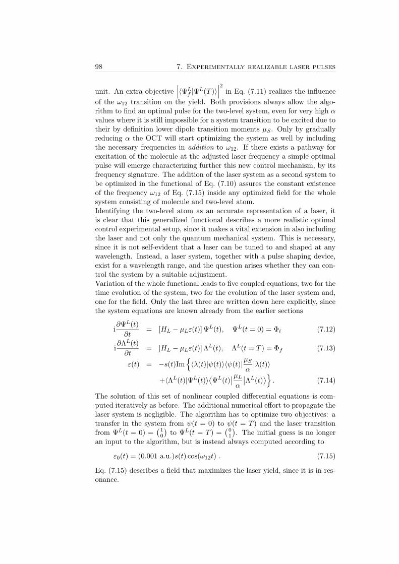
98 7. Experimentally realizable laser pulses
unit. An extra objective∣∣∣〈ΨL
f |ΨL(T )〉∣∣∣
2in Eq. (7.11) realizes the influence
of the ω12 transition on the yield. Both provisions always allow the algo-rithm to find an optimal pulse for the two-level system, even for very high αvalues where it is still impossible for a system transition to be excited due totheir by definition lower dipole transition moments µS . Only by graduallyreducing α the OCT will start optimizing the system as well by includingthe necessary frequencies in addition to ω12. If there exists a pathway forexcitation of the molecule at the adjusted laser frequency a simple optimalpulse will emerge characterizing further this new control mechanism, by itsfrequency signature. The addition of the laser system as a second system tobe optimized in the functional of Eq. (7.10) assures the constant existenceof the frequency ω12 of Eq. (7.15) inside any optimized field for the wholesystem consisting of molecule and two-level atom.Identifying the two-level atom as an accurate representation of a laser, itis clear that this generalized functional describes a more realistic optimalcontrol experimental setup, since it makes a vital extension in also includingthe laser and not only the quantum mechanical system. This is necessary,since it is not self-evident that a laser can be tuned to and shaped at anywavelength. Instead, a laser system, together with a pulse shaping device,exist for a wavelength range, and the question arises whether they can con-trol the system by a suitable adjustment.Variation of the whole functional leads to five coupled equations; two for thetime evolution of the system, two for the evolution of the laser system and,one for the field. Only the last three are written down here explicitly, sincethe system equations are known already from the earlier sections
i∂ΨL(t)
∂t= [HL − µLε(t)] ΨL(t), ΨL(t = 0) = Φi (7.12)
i∂ΛL(t)
∂t= [HL − µLε(t)] ΛL(t), ΛL(t = T ) = Φf (7.13)
ε(t) = −s(t)Im
〈λ(t)|ψ(t)〉〈ψ(t)|µSα|λ(t)〉
+〈ΛL(t)|ΨL(t)〉⟨ΨL(t)
∣∣µLα
∣∣ΛL(t)
⟩
. (7.14)
The solution of this set of nonlinear coupled differential equations is com-puted iteratively as before. The additional numerical effort to propagate thelaser system is negligible. The algorithm has to optimize two objectives: atransfer in the system from ψ(t = 0) to ψ(t = T ) and the laser transitionfrom ΨL(t = 0) =
(10
)to ΨL(t = T ) =
(01
). The initial guess is no longer
an input to the algorithm, but is instead always computed according to
ε0(t) = (0.001 a.u.)s(t) cos(ω12t) . (7.15)
Eq. (7.15) describes a field that maximizes the laser yield, since it is in res-onance.

7. Experimentally realizable laser pulses 99
By performing optimizations with this new functional for different ω12 it isfor the first time possible to show up in an isolated fashion one pathwayafter another for a single objective in the system under consideration. Theoptimal pulse has a clear structure and a mixture of all pathways shadowingeach other is avoided. This new feature is illustrated in Figs. 7.4(a) and7.4(b). In Fig. 7.4(b) the optimum electric field spectrum is depicted, wherethe initial guess center frequency ω12 was tuned to 11 698 cm−1 correspond-ing to the location of one of the most prominent peaks in the spectrum ofFig. 7.3(b). This optimal laser tuning allows for the highest α values andthe least supplementary frequencies. A system yield of 94% was reachedwith α = 2000 [see Fig. 7.4(b)]. The initial guess pulse for these two datasets was the same, but the new functional allowed for higher α values. Notethe similarity of the optimized pulse spectra Fig. 7.3(b) and Fig. 7.4(b). InFig. 7.4(a) the spectrum of the optimized field is shown for a laser frequencyω12 = 10 974 cm−1, which is detuned from optimum. The initial guess isautomatically calculated through Eq. (7.15). At α = 1300 a system yield of96% is reached. It has to be noted that although the initial guess pulses arethe same for the data in Fig. 7.3(a) and Fig. 7.4(a), the new formulationof the functional allows an α value three times higher than in the standardfunctional (α = 400). Again due to the high value of the penalty factorthe intensity of the pulse is considerably reduced to maximum amplitude of0.0002 a.u. (or intensity of 109 W/cm2). The four extra remote frequencybands are essential and cannot be suppressed. This was tested by graduallydecreasing the penalty factor from the value where only the laser transitionfrequency can exist. The algorithm for calculating the necessary mask pat-tern explained in section 7.1 was applied and resulted in the transmissionand retardance mask functions of Figs. 7.4(α) and 7.4(β). The colors markthe regions were the phase behavior is important due to significant spectralintensity.The new functional in combination with the Krotov method of building thenew field without memory behaves similarly to the modified Krotov methodwith the difference that Eq. (7.14) is a correction equation to the initialguess field which is εini
ε(t) = εini(t)− s(t)Im
〈λ(t)|ψ(t)〉〈ψ(t)|µSα|λ(t)〉
, (7.16)
with
εini(t) = −s(t)Im
〈ΛL(t)|ΨL(t)〉⟨ΨL(t)
∣∣µLα
∣∣ΛL(t)
⟩
. (7.17)
Clearly this is different from the modified Krotov (see section 5.1), where thecorrection is applied to the field of the previous iteration. In other words onecould say that in modified Krotov the memory lasts only one iteration, whilein the new functional the memory of the beginning is kept. As a result in

100 7. Experimentally realizable laser pulses
Figure 7.4: Optimal fields calculated with the generalized functional for two dif-ferent laser source center frequency tunings indicated as white arrows. (a) ω12 =10 974 cm−1. (b) ω12 = 11 698 cm−1. (α) Mask pattern of (a). (β) Mask patternof (b). Here |M(ω)| denotes the transmission and arg[M(ω)] the phase of the maskpattern. Only the colored regions of the phase mask are important, since only thereconsiderable spectral amplitude is transmitted through. Within the colored phaseregions red section are most important, while blue are less important.
modified Krotov the laser transition frequency can vanish, while it can not,when using Eq. (7.14) since an additional yield term for the laser systemthat needs the initial guess is included in the functional [see Eq. (7.10)].The functional presented here is even able to control the amount of spectralfrequency at the laser transition within the optimal pulse, by controlling µL
and thus is more general.Besides of the previously discussed features, the functional of Eq. (7.10) isthe first step towards controlling simultaneously multiple objectives witha single laser pulse. It was already mentioned that Eq. (7.10) leads toan OCT variant, that optimizes the light field of the laser source and thesystem simultaneously for low enough α. This idea can be generalized andit is possible to assume even more objectives in the same system [134] or

7. Experimentally realizable laser pulses 101
more generally in different systems
J =∑
k,s
∣∣∣〈ψk,sf |ψk,s(T )〉
∣∣∣
2− 2Re
[
〈ψk,sf |ψk,s(T )〉
T∫
0
dt⟨
λk,s(t)∣∣∣
[
i(Hs − µsε(t)) + ∂
∂t
]∣∣∣ψk,s(t)
⟩]
. (7.18)
This equations will deliver an optimal pulse for the transfer into k targetstates starting from m (≤ k) initial states in s different systems, incoherentlyfrom one another. Incoherent because the absolute value of each individualtarget is taken as objective and not the absolute value of their sum. Variationof this functional gives equations similar to Eqs. (7.12)-(7.14)
i∂tλk(t) = [Hs − µsε(t)]λk(t), λs(t = 0) = φmi (7.19)
i∂tψk(t) = [Hs − µsε(t)]ψk(t), ψk(t = T ) = φkf (7.20)
ε(t) = −s(t)α
∑
k
Im
〈λk(t)|ψk(t)〉⟨
ψk(t)∣∣∣µs∣∣∣λk(t)
⟩
. (7.21)
A possible application of this very general functional is to solve the problemof molecular π-pulses, that invert an initial Boltzmann distribution. Anotherrecent application of this functional is the design of laser pulses suitable formolecular quantum computing [135], where operation of a single pulse onseveral qubits is required.In conclusion new strategies to reduce the complexity of pulses obtainedby the OCT algorithm and to discover new control mechanisms were de-veloped. The parameter α is of critical importance if robust pulses are tobe retrieved. A new formulation of the functional including the laser sys-tem, allows high α values and therefore produces immediately spectrallypurified pulses. These robust pulses are amenable to a detailed study andtheir experimental realization is an easy task with state of the art pulseshaping technology. The new, more general functional can be used to distillall optimal control pathways for an objective by tuning the laser frequency.The pathways are thereby made accessible to a more detailed study. Thispowerful tool can be used to clear off complex excitation patterns and dis-cover new optimal control processes in quantum mechanical systems, sincethe solutions will always include the laser frequency and be as simple aspossible.
7.4 Projector method
The aim of this section is to derive a new OCT functional that providesoptimal pulses with a pre-specified spectral width and leading to coupled

102 7. Experimentally realizable laser pulses
equations still solvable with the closed loop iteration scheme.In the early formulation of the OCT algorithm a filtering technique [31] wasproposed to restrict the optimal fields to a specified frequency bandwidth(see introductory remarks to chapter 7). This technique cannot be appliedwithin the framework of closed equations [Eqs. 5.7,5.9 and 5.10]. The electricfield in the closed form iteration is calculated at each step and not in a one-cycle-to-next-cycle (one cycle of iteration includes a number of steps) style asin gradient type methods (see discussion in section 5.1). Therefore a spectralconstraint using filtering in the Fourier domain can only be applied at theend of the iteration cycle, where the complete spectral information of thepulse is present. Consequently the algorithm has felt no spectral constraintduring the whole cycle and application of the filter would only disturb theconvergence. In the following a new functional is presented which allows forspectral pressure also within this closed form, rapidly convergent OCT.
In order to derive the new functional, that allows to include spectralpressure, the following idea is central. The electric field is essentially buildfrom the overlap of populated eigenstates of the field free Hamiltonian [seeEq. (5.10)]. Even if the wave function is represented on a grid its eigenstatecomposition can be obtained through projection. The spectral width of theoptimal pulse is controlled indirectly by allowing the wave functions ψ andλ to consist only of a pre-specified set of eigenfunctions. The idea behindthis reduction of the number of eigenstates contributing to a wave packetis, that a spectrally broad pulse will excite coherently many eigenfunctions,while a spectrally narrow pulse will excite only a few eigenfunctions at anytime. The projection of the wave function on the constituting vibrationaleigenstates at three different times and for three excitation pulses with afwhm of 10 fs, 50 fs and 100 fs is shown in Fig. 7.5. Clearly the width of thedecomposition greatly reduces as the pulse becomes of smaller bandwidth.Therefore an intelligent reduction of contributing eigenstates in Eq. (5.10)will reduce the number of transitions with different frequencies and hencethese frequencies will be the only ones appearing in the pulse spectrum.To be more specific let us consider an optimal transfer in the potassiumdimer involving only the X and A state and their vibrational levels. Takingthe case that the initial state is a single vibrational eigenstate the spectralwidth can be simply controlled by allowing only vibrational levels aroundthis initial state (set X) and a set of vibrational levels in the A state (set A).The choice of these two eigenstate sets will specify the center wavelengthand spectral width of the pulse. The maximum frequency will be given bythe transition between the lowest eigenstate in set X and the highest in setA, while the minimum allowed frequency is simply the difference of energiesbetween the highest energetic eigenstate in set X and the lowest in set A.Since the sets X and A can be chosen arbitrarily, for instance they do nothave to be connected, the spectrum of the pulse can be arbitrarily tailored.Indeed only a not-connected set X will allow pump-dump pulses with very

7. Experimentally realizable laser pulses 103
Figure 7.5: A state wave packet decomposition in eigenstates at initial, interme-diate and final time for excitation with three different pulse durations.(a) 10 fs (b)50 fs and (c) 100 fs. Each line depicts a snapshots of the wave function at onespecific time.
different frequencies of the pump and dump step. Similarly to the shapefunction s(t) that influences the appearance of the optimal pulse envelope ashape function on the eigenstates will mold the pulse spectrum.If P is the projector onto the subsets of eigenstates and P the projector onall other eigenfunctions, the relation 1 = P + P holds true. This relation isused to split Eq. (5.10) into two summands ε(t) = ε(t)y + ε(t)n, where thefirst summand is the spectrally small part, while the other with superindexn contains further spectral components to be eliminated.
α
s(t)ε(t) = −Im
N∑
k,l=1
W (l)2a†il afkδkl
N∑
k,l=1
W (l)W (k)〈vl|a†fl µaik|vk〉
︸ ︷︷ ︸
ε(t)y
−Im
∞∑
k,l=N+1
. . .
∞∑
k,l=N+1
. . .
︸ ︷︷ ︸
ε(t)n
. (7.22)
Here the complex numbers ail(t) = 〈vl|ψi(t)〉 have been used. Consideringonly the term ε(t)y leads to the new OCT algorithm with spectral restric-tion. The closed equations for λ and ψ itself are the same as before withthe exception of the equation for ε(t) which has changed into Eq. (7.22).Numerically this formula is implemented by applying the projector on bothwave functions ψi(t) and ψf (t) each time a new point of the electric field iscalculated through Eq. (5.10), i.e. at each time step of the iteration. Theseprojected wave functions are only used to construct the electric field. Thepropagation is continued with the original unprojected wave functions for

104 7. Experimentally realizable laser pulses
the next time step followed again by the projection step. This process is re-peated until the end of the cycle. Propagation on a grid as is performed hereneeds the original wave functions to be propagated and not the projectedones, since this would lead to the destruction of convergence. Thereforethe projector can not be included directly in the Schrodinger equation con-straint of Eq. (5.8). Alternatively, when all eigenfunctions are known andnot only the ones needed for the projector in Eq. (7.23), the propagationcan be performed directly in the basis of eigenfunctions and not on a grid.In the case of the potassium dimer about 30 vibrational eigenstates of eachelectronic state are needed to achieve the same numerical results as with agrid of 256 points. A reduced set of eigenfunctions can be used only in theprojector to evaluate the electric field according to Eq. (7.22), but not forthe propagation of the molecular system.
The iterative scheme is started by taking as a favorable initial guess theoptimized pulse from an unconstraint OCT run. After convergence themask function can be extracted from the spectrum of the optimal pulse byusing Eq. (7.6). Since the spectral width of the optimal pulse is controlledwith the parameter ∆v in the shape function W, the number of pixels canbe reduced drastically. It is now possible to design experimentally realizablepulses with this OCT variant that controls the spectral width of the optimallaser pulse. Moreover it is a fast and efficient code for providing optimallyshaped pulses which can directly serve as input to the experiment. Spectralpressure also tends to simplify the laser pulse features, enabling the extrac-tion of the control mechanism.Just to show that this works, the population transfer from v′′ = 0 (|v′′0〉)to v′′ = 2 (|v′′2〉) in the ground state using the first electronic excited stateA 1Σu as an intermediate pathway will serve as prototype control. It is notnecessary to define a projector in the ground state, since initial and targetvibrational state are within the bandwidth of a 50 fs pulse. Only a projectoronto a specified subset of N excited state vibrational eigenfunctions |vn〉 ofthe field free Hamiltonian H0 is defined and weighted with a shape functionW(n)
P =N∑
n=1
W (n)|vn〉〈vn|. (7.23)
The shape function was chosen to be a Gaussian distribution
W (n) = exp
−(v − v0
∆v
)2
. (7.24)
Here v0 is the maximum and ∆v is the width of the desired eigenfunctiondistribution. In the extreme case v0 = 6 and ∆v = 3 was selected, which

7. Experimentally realizable laser pulses 105
corresponds to a pulse at ≈ 820 nm with spectral bandwidth correspondingto 50 fs.The results are shown in Fig. 7.6. The yield y is defined as the overlap withthe target eigenfunction
y = |〈ψi(t = T )|φf 〉| or alternatively as y = |〈ψf (t = T )|φi〉|, (7.25)
where |φi〉 = |v′′0〉 and φf = |v′′2〉. The first column shows a pulse calcu-
Figure 7.6: Optimal control pulses transferring population from v′′ = 0 to v′′ = 2in the ground state using the first electronic excited state A 1Σu as an intermediatepathway. Each column depicts one optimal pulse, retrieved by gradually increasingspectral pressure. (a)-(c) pulse envelope. (α)-(γ) pulse phase. (1)-(3) STFT of thepulse.
lated with OCT using no spectral restriction. The optimized pulse producesa yield of 0.94. The FL pulse from which the shaped pulse originates hasa duration of 10 fs and a complex mask pattern with a number of pixelsexceeding the usual experimental number of 128 [see Fig. 7.7(a)]. Whenspectral pressure is applied by reducing the parameter ∆v the optimal fieldbecomes more robust, but efficiency is gradually reduced. These results areshown in Fig. 7.6(a) and 7.6(b), respectively. Interestingly some spectralpressure can be applied without loosing much efficiency (b). This pulse stillhas a yield of 0.92 with the advantage of having a spectrum correspondingto a longer pulse of 20 fs and a realizable mask pattern [see Fig. 7.7(a) and7.7(b)]. Figure 7.6(c) shows a pulse that has a yield of 0.76, and is eveneasier to shape due to its 40 fs FL duration and simplex mask pattern [Fig. 7.7(c)]. The pulse consists of a clearly structured pulse sequence, wherethe third pulse is linearly negatively chirped.The difference of the projector and the new functional method is best ex-plained in view of its application. The projector method should be used,

106 7. Experimentally realizable laser pulses
Figure 7.7: Transmission |M(ω)| and phase arg[M(ω)] of the mask patternsneeded to tailor the pulses of Fig. 7.6. (a) Is the mask pattern for the pulse inFig. 7.6(a), (b) for the pulse in Fig. 7.6(b) and (c) for the pulse in Fig. 7.6(c).
when the spectral shape, especially bandwidth, shall be constraint. Thepulse simplicity can be adjusted by the spectral width of the projectors andit is best to use very low values for α. Since the algorithm is not able tosearch freely for the most robust pathways and is instead constraint to theallowed frequencies, the optimal pulse must have sufficient energy to excitethe allowed, but perhaps non-optimal pathways.The new functional answers the question what extra frequencies besides thelaser center frequency are needed to optimize the target, that is which is themost efficient transfer mechanism for a given laser source. The new func-tional provides more potential applications, it can also be applied whenevera electric field is sought that optimizes several targets at once. The maindifference to the method of this section is the impossibility to constrain thenew emerging frequencies to a specified spectral window. Using the algo-rithm of the past section appropriately means to start with high α valuesand reduce the α parameter to enable a growth of the frequencies in theoptimized pulse until the desired yield is achieved. The optimized pulseobtained by the method of section 7.3 has always the lowest possible pulseenergy, just enough to excite the most robust pathways out of the excitationregion selected by the center frequency of the laser source.

Chapter 8
Application
In the following two sections simple femtosecond laser pulses are obtainedusing the method of section 7.2 for the SST and PI transfer introduced inchapter 6.
8.1 State selective population transfer (SST)
In this section the efficient femtosecond-laser induced transfer of populationbetween two eigenstates of the ground electronic state is investigated. Bothstates must be connected via the first electronically excited state since adirect IR transition is forbidden due to the homonuclear character of thepotassium dimer. Earlier work [136] has shown that this system can beeffectively treated as a lambda system if nanosecond or continuous wavelasers are used. In this realm STIRAP can be efficiently used. Here acompletely different regime is investigated, where the applied pulses havea broad frequency spectrum coherently exciting a superposition of manyeigenstates, but as will be shown are still selective to a single eigenstatedue to their proper pulse shape. Moreover the simultaneous excitation ofmany eigenstates makes the problem not reducible to a simple lambda sys-tem. This conceptual formulation is appropriately solved with the rapidlyconvergent OCT (see section 5.1), which naturally excludes the counterintu-itive STIRAP solutions since only frequencies of populated levels constitutethe pulse during the iterations. The results extend previous work of ourgroup [115].
Single well defined initial state. The powerful method of highpenalty factor optimization allows to deduce the control mechanism behindthese optimal pulses by merely looking at their short-time Fourier transform.A comparison of the STFT of the pulse transferring above 90% of the popu-lation from v′′ = 0 to v′′ = 2 [Fig. 8.1(a)] with the pulse doing this for v′′ =
107

108 8. Application
0 to v′′ = 5 [Fig. 8.1(b)] reveals a Tannor-Rice-Kosloff pump-dump mecha-nism. The pump and dump frequencies differ by the energy spacing betweeninitial and target vibrational state and the overlap in time of the subpulsesis bigger in the case of v′′ = 0 to v′′ = 5. The correct time separation, phaseand center frequencies of the subpulses lead to a pump-dump mechanismthat is vibrationally state selective at final time. Figure 8.2 shows snap-
Figure 8.1: Pulses optimizing transfer between two eigenstates of X 1Σg via A1Σu. (a) v
′′ = 0 to v′′ = 2. (b) v′′ = 0 to v′′ = 5.
shots of the wave packet during the optimal v′′ = 0 to v′′ = 2 transfer onthe grid 8.2(a)-(d) and its projection onto eigenstates 8.2(α)-(δ). At inter-mediate times [Figs. 8.2(b) and (c)] the ground state wave packet consistsof a coherent superposition of eigenstates, while at initial and final time itis a single eigenstate of the field free Hamiltonian. The pulse is hence tai-lored to be selective to states within its excitation bandwidth. The Ramanpumping realized between moving wave packets on the potential surfaces, issuch that population ends again in the ground state and is concomitantlyshaped into an eigenstate. Once the target wave packet has the shape ofan eigenstate it will also have its energy. There remains some populationin high energy ground eigenstates, since the transfer is not complete, thatis 100%. The population in the higher excited potentials is negligible andessentially the pulse couples only the two lowest electronic states, X andA. This is general to all eigenstate transfers with moderate ∆v, since theoptimal pulses all have low peak amplitude on the order of 2 10−4 a.u. (=an intensity of 109 W/cm2) [see Figs. 8.3(a) and 8.4(a)-(d)]. The effect ofphase in this transfer was also investigated. The subpulses of the tailoredv′′ = 0 to v′′ = 5 laser field [Fig. 8.3(a) and its spectrum Fig. 8.3(α)] arecalculated, by extracting from all Fourier components the ones belonging tothe pump and to the dump frequency [115,137]. The resulting subpulses areshown in Figs. 8.3(b) and (c). Clearly the earlier pulse has the higher fre-quency and serves as pump, while the later pulse dumps the population [see

8. Application 109
Figure 8.2: One dimensional wave packet propagation, showing snapshots of theoptimal v′′ = 0 to v′′ = 2 transfer.(a)-(d) grid representation of the wave function.(α)-(δ) eigenfunction representation of the wave function.
Fig. 8.3(βγ)]. Having calculated the subpulses it is possible to combine themagain to a single pulse using a method described in Ref. [115,137]. Therebytheir relative phase can be changed, by adjusting the absolute phase of oneof the pulses relative to the other. A change in phase just shifts the carrierwith respect to the envelope and when combining with the other subpulsewill lead to a phase dependent interference in the temporal overlap regionof the two pulse constituents. The combined pulse is then propagated and aplot of phase versus yield can be generated [Fig. 8.3(1)] and shows a periodicmodulation with a maximum yield at 1 rad. The maximum yield is below95% since the spectrum of the combined pulses coincides only in the maintwo frequencies and thus is only an approximation to the original pulse ofFig. 8.3(a).Another peculiarity of the eigenstate transfer with femtosecond pulses is
that whenever v′′ = 0 is involved the optimal pulse is more complex andlooses its time symmetry. This can be inferred from Fig. 8.4, where theoptimal laser fields 8.4(a)-(d) and their spectra 8.4(α)-(δ) are plotted.Here the transfers with ∆v = 2 between v′′=0 to v′′=2 [Figs. 8.4(a) andα] and v′′=2 to v′′=4 [Figs. 8.4(b) and β] and ∆v = 4 from v′′=0 to v′′=4[Figs. 8.4(c) and (γ)] and v′′=4 to v′′=8 [Figs. 8.4(d) and (δ)] clearly showthat whenever v′′ = 0 is involved the laser field is asymmetric in time and the

110 8. Application
Figure 8.3: (a) Laser pulse optimized for v′′=0 to v′′=5. (b) and (c) are itssubpulses. (α) Spectrum of pulse (a) and (βγ) spectra of the subpulse (b) in blackand subpulse (c) in gray. (1) Change of the yield as a function of the phase-relationship of the subpulses.
pump and dump frequencies show both a doublet. Inspection of Figs. 8.4(β)and 8.4(δ) reveals that the dump frequency in Fig. 8.4(β) and the pumpfrequency in Fig. 8.4(δ) coincide. The control process uses the same inter-mediate excited vibrational states for the transfer.Another aspect to be considered in the following is the maximum value
achievable for ∆v in this kind of transfer. The larger ∆v is chosen thesmaller is the Franck-Condon factor connecting both states. However it isstill possible to transfer population from vibrational states near the dissocia-tion continuum to v′′ = 0 of the ground singlet potential. This kind of trans-fer is one of the key steps for conversion of a Bose-Einstein-condesate(BEC)of atoms to a molecular BEC (or MBEC) [138,139] with ultrashort coherentpulses as proposed in section 11.2.3. Methods so far proposed use STIRAPas a very effective and selective process to complete this task [140–143]( seealso section 11.2). The total number of bound states in a potential dependscritically on its depth and for the available ab initio X and A potentials thenumber of bound states in X was calculated to be 85 while it is 195 for theA state. As an initial eigenstate near dissociation v′′ = 80 was chosen, whilethe final state is v′′ = 0. This calculation was performed in the eigenstatebasis taking into account all bound vibrational eigenstates of the X and A

8. Application 111
Figure 8.4: Laser pulses optimizing different eigenstate transfers. (a) v′′ = 0 tov′′ = 2. (b) v′′ = 2 to v′′ = 4. (c) v′′ = 0 to v′′ = 4. (d) v′′ = 4 to v′′ = 8. Theircorresponding spectra are in (α)-(δ).
potential1). Assuming a direct transfer to a vibrational state in the excitedpotential and back down to the final state, the effective transition dipolemoment for this transfer is highest for v′ = 41, but is three orders of mag-nitude smaller than the strongest transition in K2. Nevertheless it is stillpossible to accomplish this transfer by a two-step process. The STFT of thepulse is depicted in Fig. 8.5(a) for low α and 8.5(b) for high α. Again it
Figure 8.5: Laser pulse optimized for v′′=80 to v′′=0. (a) Optimization with lowand (b) with high penalty factor.
1)A grid based method would have been only effective with a nonlinear grid mapping
to reduce the number of necessary points to accurately support the wave packet dynamics
near dissociation.

112 8. Application
is most simple to derive the central mechanism by inspecting the laser fieldFig. 8.5(b). It consists of two main frequency bands at 12 000 cm−1 and14 000 cm−1 and a less pronounced around 9 500 cm−1. A time resolvedanalysis reveals, that the optimal transfer proceeds via a two-step process.First the population is transferred to an intermediate level (around v ′′ = 40)and from their down to v′′ = 0. This optimal process does not proceed overv′ = 41, but over v′ = 140 [see Fig. 8.6(β)] enhancing thereby the transitiondipole moment of the overall process. In order to verify the tailored pulses
Figure 8.6: One dimensional wave packet propagation, showing snapshots of theoptimal v′′ = 80 to v′′ = 0 transfer. (a)-(d) grid representation of the wave function.(α)-(δ) eigenfunction representation of the wave function.
for the SST transfer in experiment a beam of molecules or the preparation ofa single vibrational state in an excited potential [144] would be the methodof choice. Here the initial state would be well defined and coinciding withthe assumptions made in theory.Nevertheless an experimental setup using an heat pipe oven, where the alka-lis are simply evaporated, is less involved. Here the dimers in the gas phaseconstitute a thermal ensemble. This case will be studied next.
Thermal ensemble initial state. The following calculations howevershow that it is still possible to have an experimental signature for an optimaleigenstate transfer even in a thermal ensemble. The main reason for thisis that the anharmonicity of the vibrational ladder is high enough that an

8. Application 113
optimized pulse will be efficient only between the specified initial and targeteigenstate and not generally between vibrational eigenstates spaced by thesame number of quanta. That is a pulse optimized for v′′ = 0 to v′′ = 2 isnot optimal for v′′ = 2 to v′′ = 4. The clear difference in the optimal pulseswas already shown in Figs. 8.4(a), 8.4(α), 8.4(b) and 8.4(β). The calcula-tions assume an initial Boltzmann distribution over 16 vibrational states inthe ground state. In Fig. 8.7(c) the final ground state population is plotted,for a tailored pulse optimized for v′′ = 0 to v′′ = 1 [Fig. 8.7(a)] and thecorresponding bandwidth limited pulse [Fig. 8.7(b)]. A distinguished peak
Figure 8.7: Thermal ensemble of K2 is excited with laser pulse optimized withlow α for the transfer from v′′=0 to v′′=1. (a) The optimized electric field. (b)The corresponding Fourier limited laser pulses. (c) Final ground state distributioninduced by laser pulse (a) in gray and (b) in black.
at v′′ = 1 rises above an else nearly flat unstructured ground state popula-tion. Clearly the two vibrational distributions would be distinguishable inexperiment and the tailored pulse could be identified as optimizing v′′ = 0to v′′ = 1. As long as the Fourier limited pulse used to shape the optimalpulse is of broad bandwidth a clear signature is visible for a whole range ofeigenstate transfers. This beautiful signature vanishes however if the band-width of the tailored laser pulse is in the regime of bandwidth limited 100fs pulses [see Fig. 8.8(c)]. This can be shown by propagating the v′′ = 0 tov′′ = 1 obtained in a high α OCT run [Fig. 8.8(a)]. This simple pulse canbe shaped from a 100 fs Fourier limited pulse [Fig. 8.8(b)].In a further example the possibility is considered of optimizing a pulse thattransfers all the population from v′′ = 0 to a specified vibrational superposi-tion state in the first excited potential. The population of the excited statewill then reveal the eigenstate composition of the wave packet, despite theinitial Boltzmann distribution of states [see Fig. 8.9(c)]. The two distinctpeaks show evidence that the specified target state here is a superpositionstate with v′ = 2 and v′ = 4 contributions. The signature again nearlyvanishes if a simple pulse optimized for the same target is to be used (notshown). Therefore the control will be very hard to detect in experimentusing molecular gas cells with pulses above fwhm of 10 fs.
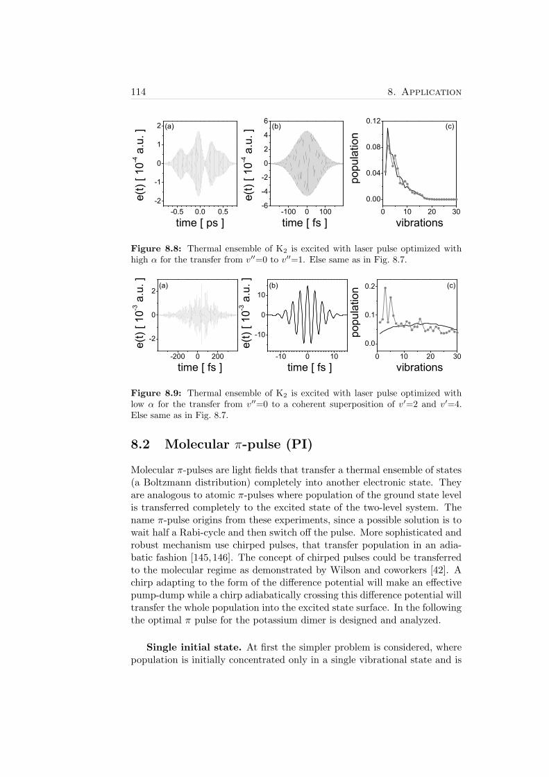
114 8. Application
Figure 8.8: Thermal ensemble of K2 is excited with laser pulse optimized withhigh α for the transfer from v′′=0 to v′′=1. Else same as in Fig. 8.7.
Figure 8.9: Thermal ensemble of K2 is excited with laser pulse optimized withlow α for the transfer from v′′=0 to a coherent superposition of v′=2 and v′=4.Else same as in Fig. 8.7.
8.2 Molecular π-pulse (PI)
Molecular π-pulses are light fields that transfer a thermal ensemble of states(a Boltzmann distribution) completely into another electronic state. Theyare analogous to atomic π-pulses where population of the ground state levelis transferred completely to the excited state of the two-level system. Thename π-pulse origins from these experiments, since a possible solution is towait half a Rabi-cycle and then switch off the pulse. More sophisticated androbust mechanism use chirped pulses, that transfer population in an adia-batic fashion [145, 146]. The concept of chirped pulses could be transferredto the molecular regime as demonstrated by Wilson and coworkers [42]. Achirp adapting to the form of the difference potential will make an effectivepump-dump while a chirp adiabatically crossing this difference potential willtransfer the whole population into the excited state surface. In the followingthe optimal π pulse for the potassium dimer is designed and analyzed.
Single initial state. At first the simpler problem is considered, wherepopulation is initially concentrated only in a single vibrational state and is

8. Application 115
transferred by a suitably tailored pulse into the A1Σu state. A summary ofthe resulting pulses starting from different initial states is shown in Fig. 8.10.Obviously the optimal pulses depend on the initial state. Figures 8.10(a)and 8.10(d) and also Fig. 8.10(c) and Fig. 8.10(f) bear near resemblance andare extremely ordinary consisting of a double or a single pulse, surroundedby two small amplitude pulses, at the same center frequency. Figures 8.10(b)and 8.10(e) are an intermediate case, where two main frequencies seem tobe more favorable for an efficient transfer.
Thermal initial state. Using the new functional introduced in sec-tion 7.3 it is now possible to obtain a real molecular π-pulse. The initialpopulation is exemplarily taken to be a thermal distribution involving fivevibrational states in the ground state of K2. In this case s=1, k=m=5 inequation 7.19. As target of the optimization the projector onto the first
Figure 8.10: STFT of pulses that transfer population concentrated initially withina vibrational ground eigenstate v′′ into A 1Σu. Population is initially in (a) v′′=0.(b) v′′=1. (c) v′′=2. (d) v′′=3. (e) v′′=4. (f) v′′=5.
excited electronic state (A) is considered. The resulting optimal pulse isshown in Fig. 8.11. It has a nonlinear positive chirp and differs considerablyfrom each of the optimal pulses that invert only the population of one singlevibrational state [see Figs. 8.10(a)-(f)]. Therefore it can not be obtained bysimply averaging over all these pulses.

Figure 8.11: Molecular π-pulse transferring a initial Boltzmann distribution offive vibrational ground states v′′ = 0. . .5 into A 1Σu.
116

Chapter 9
Comparison experiment andtheory
9.1 Rotation and orientation effects
The motivation for studying the ro-vibronic motion of potassium dimers istwofold. It is known from earlier work [147] that rotation can harm controland it is important to quantify this effect for the SST control of K2 studied insection 8.1. Moreover a direct comparison with experimental results is onlypossible if the rotational degree of freedom is considered besides the alreadytreated initial thermal distribution (see section 8.2). In this section the effectof the molecular rotation on the selective population transfer between vi-brational levels is studied with shaped femtosecond pulses. The populationdistribution within the rotational levels of one vibrational level can not becontrolled, i.e. selective control over ro-vibronic levels with these broadbandpulses is impossible, since the rotational spacing is ten times smaller thanthe vibrational energy spacing. This can be understood by rethinking aboutthe control mechanism found to be responsible for state selective controlover vibrations. There control was achieved by consecutive pumping anddumping of population between moving vibrational wave packets on bothelectronic states. A considerable nuclear motion during the pulse action isessential. Rotational wave packets move about ten times slower, their mo-tion lying in the picosecond regime. This however means that a tailoredfemtosecond pulse would have to extend over several picoseconds in order tocontrol by the same mechanism as found for the mere vibrational motion.This is experimentally difficult to realize.Following this argument of time scale separation one would expect only aminor effect of the rotations on vibrational control. However for K2 a fur-ther complication arises, that is harmful for control. The transition-dipolemoment lies along the internuclear axis. Consequently if the dimer is ori-ented orthogonal to the field the laser control over the molecule vanishes,
117

118 9. Comparison experiment and theory
since the dipole moment for this orientation is zero. While the dynamics ofrotations are slow their effect can still be important since the rotating dipolevanishes for orthogonal orientation to the external laser field. The theoret-ical calculations in this section are therefore an extension to earlier studieswhere only the static orientation of the molecule with respect to the fieldwas considered [35]. Alignment by the laser pulse is however not consideredand its influence is studied in future work.In the following the wave function |ψ〉 is represented as a vector in theelectronic components (X,A,2,4). The Schrodinger equation can be solvedeither in coordinate space or in the eigenfunction representation. For com-pleteness, the full spherical Hamiltonian for the ro-vibronic description isexplicitly written down in both representations. On the grid the Hamilto-nian is:
i∂t〈x|χ〉 =−~2
2m
[
∂2r +
1
r2
(
∂2φ
sin2(θ)+ cot(θ)∂θ + ∂2
θ
)]
〈x|χ〉
+ 〈x|Vint(ε)|x〉〈x|χ〉 . (9.1)
where the usual definition 〈x|χ〉 = r〈x|ψ〉 was used. This Hamiltonian isthree dimensional since the bond length r and the angles θ,φ specifying theorientation in space of the molecule with respect to the laser field is consid-ered. The interaction with the laser corresponds to the following matrix
〈x|Vint(ε)|x〉 = ε(t) sin(θ) |X〉µXA(r)〈A|+ |A〉µA2(r)〈2|+ |A〉µA4(r)〈4|+ c.c. . (9.2)
Here the dipole moments between the electronic states i, j must be evaluatedin the coordinate representation: 〈x||i〉µijε(t)〈j||x〉 = ε(t) sin(θ)|i〉µij(r)〈j|as the dipole moments are only r dependent. In the eigenfunction represen-tation the Schrodinger equation is [148]
i∂t〈nvlm|ψ〉 = Enls〈nvlm|ψ〉+
∑
n′v′l′m′
〈nvlm|Vint∣∣n′l′v′m′
⟩〈n′v′l′m′|ψ〉 . (9.3)
⟨n′v′l′m′
∣∣Vint(ε)|nvlm〉 = ε(t)
|X〉〈A|µnX lX ,nAlAXA
+ |A〉〈C|µnAlA,nC lCAC
+ |A〉〈D|µnAlA,nDlDAD + c.c.
(9.4)
The quantum numbers stand for: n - electronic state, v - vibration, l - or-bital angular momentum and m - eigenvalue of the lz component. The dipoletransitions moments are calculated by a product of dipole matrix element

9. Comparison experiment and theory 119
and the coefficients al,m =√
(l+m+1)(l−m+1)(2l+1)(2l+3) describing the orientation of
the molecule relative to the laser [149]. The ro-vibronic eigenstates werecalculated by a Numerov scheme on the centrifugally distorted potentials ofthe mere vibrating potassium molecule. They are in good agreement withspectroscopic data. The number of ro-vibronic eigenstates in each potentialused in the expansion of the wave function was increased until the propaga-tion data faithfully converged into agreement with the results on the grid.Since the rotational quantum number is a also measure for the laser fieldinteractions, it is interesting to note that 15 rotations per vibration wereneeded for accurate results.As a linearly polarized control laser is assumed, the selection rules ∆m = 0(lz is conserved) and ∆l = ±1 hold. Throughout this work a l′′ = 0 (whichimplies m′′ = 0) ro-vibronic eigenstate served as initial state. Therefore thequantum number remains always m = 0, which is equivalent to ignoring the∂φ term on the grid.The grid calculations reduce to an effective two dimensional problem withonly the bond length r of the diatom and θ the orientation angle of themolecule with respect to the laser. In the two-dimensional calculations thedipole transition moment was taken and extended to two dimensions bymultiplying with sin(θ). Here the angle θ is chosen to be in the interval0 . . . 2π, which is two times the physical range, but necessary to fulfill peri-odic boundary conditions. The number of grid points in r were 128 and 80in θ direction.The eigenfunction calculations also simplify since no sum over m has to beconsidered. The geometric coefficients al,l′,m are then evaluated to al,l+1,m=0 =〈l| cos(θ)|l + 1〉|m=0 between l and l+1 and to al,l−1,m=0 = 〈l| cos(θ)|l − 1〉|m=0
between l and l− 1. Here I recall the pure vibrational case treated in chap-
ter 8, where Eq. (9.1) simplifies to H =[−~2
2m ∂2r + 〈x|Vint(ε)|x〉
]
〈x|χ〉 andin Eq. (9.3) the quantum number of rotations l has not to be considered.Calculations in both representations, were performed. The Chebychev scheme[126] was used to numerically solve the two-dimensional non Cartesian Hamil-tonian in both space and eigenfunction representation. A second order differ-encing (SOD) approach is faster, but has dramatic instabilities when appliedto the iterative equations of OCT (see section 5.2). Instability of the SODoccurred during the forward propagation of the iterative procedure whenthe final time T reached the few ps and also for α < 100. Instead theChebychev expansion allows for a bigger time step (6.0 a.u.) and a preciseaccuracy control. Twelve expansion coefficients were used.In the following the vibrational only model will be termed 1-D and the ro-vibronic model introduced in this section as 2-D.
1-D optimized pulses applied to 2-D problem. The first step wasto investigate whether the pulses of chapter 8 are also optimal for a rovi-

120 9. Comparison experiment and theory
brating molecule. As mentioned in the introduction the degree of control isexpected to depend on the initial orientation of the molecule with respect tothe applied field. Three different orientation are considered [see Fig. 9.1(a)]:no angular orientation, sin2(θ) and the tightest orientation described by asin5(θ). At first the SST pulse optimizing the transfer from v′′ = 0 to v′′ = 2
Figure 9.1: No angular orientation (line), sin2(θ) (filled dots) and the tightestorientation described by a sin5(θ) (hollow dots). (a) Orientation before pulse action.(b) Starting from the v′′ = 0 initial state (gray line), the final v′′ = 2 state is reachedthe better the pre-orientation. (c) The better the pre-orientation the better thetransfer into the first excited electronic state.
(see section 8.1) is propagated using the ro-vibronic Hamiltonian [Eq. (9.1)].The yield is calculated as the overlap of a v′′ = 2 vibrational eigenstate withthe r-shape of the two dimensional ro-vibronic wave packet at final timeT. The r-shape is evaluated by integrating over the θ direction. The yieldachieved by these pulses is only about 50%, if the molecule is not oriented(the angular probability distribution being uniform) with respect to thelaser. This yield-loss can be attributed to the fact, that the molecule has fi-nite probability to be oriented parallel to the laser θ = 0 and θ = π, where nolaser control is possible due to the vanishing dipole moment. Outside thesenon-accessible angles the laser control still behaves as before, reshaping thei.e. initial v′′ = 0 r-shape [see Fig. 9.1(b)] into v′′ = 2. The timescale ofthe ro-vibronic movement, that reshapes the θ distribution is given by therotational energy level separation in the potassium dimer. It is thereforevery slow and a large amount of population stays at θ = 0 and θ = π within

9. Comparison experiment and theory 121
the optimization time of T =1.74 ps. Orientation of the molecule beforelaser control significantly enhances the yield. The data of Fig. 9.1(b) clearlyshows that the better the molecule is oriented in a certain direction (hereat right angles to the incident laser) the more pronounced the control. Thesame dependence of the yield on prior orientation of the molecule can beobserved for the π pulses of section 8.2 under the additional influence ofrotation. Fig. 9.1(c) shows the r-shape of the A state wave packet at finaltime. Note the increase of the norm as a function of initial orientation. Theyield for an pre-orientation even in θ is 73%, for sin(θ) is 83% and for sin5(θ)is 90%. The line styles in Fig. 9.1(b) and 9.1(c) correspond to the threeorientations of Fig. 9.1(a).
2-D optimization of SST. To improve the yield of the laser fields of sec-tion 8.1 for the two-dimensional problem, optimization with the grid basedHamiltonian of Eq. (9.1) was performed. The initial state considered isshown in Fig. 9.2(a). It is a v′′=0 state with a flat angular distribution
Figure 9.2: Snapshots of the two dimensional wave packet evolution on the gridat times (a) 0 ps, (b) 0.44 ps and (c) 1.74 ps.
(lz=0 state). The target state was defined as ψ(r, θ) = v2′′(r), constant in
θ. Figure 9.3 shows the STFT of the pulse connecting initial to final statewith a yield of 80%. The improvement of the yield compared to 56% istherefore significant. The change in shape is only minor as compared to theinitial guess pulse taken from the pure vibrational model [see Fig 8.1(a)],but exhibits less pronounced subpulses in between. The propagation dataof Fig. 9.2 shows a snapshot of the wave packet for the times (0, 0.44 ps,1.74 ps) under the action of the pulse of Fig. 9.3. The wave packet at finaltime T = 1.74 ps has a v′′=2 eigenfunction shape in r-direction, disturbedby less amount of finite uncontrollable population at θ = 0 and θ = π.

122 9. Comparison experiment and theory
Figure 9.3: STFT of the laser pulse optimized within the two dimensional modelto maximize the selective transfer from v′′ = 0 to v′′ = 2.
2-D optimization of PI transfer. Taking the π pulses of section 8.2 asinitial guess the complete inversion of population initially in the electronicground state under the influence of rotations is considered. In order tocalculate such an optimal pulse the yield term of the functional is replacedby |〈ψ|P |λ〉|2 with the projection operator P = |A〉〈A| onto the first excitedelectronic state A. It is assumed that all the ground state population isin v′′=0 l′′=0. The optimal pulse is shown in Fig. 9.4. It resembles a
Figure 9.4: STFT of the laser pulse optimized within the two dimensional modelto maximize the transfer from v′′ = 0 to A 1Σu.
phase correlated double pulse with an interpulse separation of 510 fs, thevibrational period in the A state. The pulse of Fig. 9.4 is again similar tothe corresponding π pulse [see Fig. 8.10(a)], but has a more pronouncedintensity contrast. This optimization improved the transfer efficiency in thecase of complete random orientation of the diatom from 73% achieved bythe pulse of Fig. 8.10(a) to about 87% [see Fig. 9.4].

Part III
New directions of coherentcontrol theory
123


This part is dedicated to cooling molecules, by two different methods.The first concerns cooling the internal degrees of freedom of an initially hotmolecular ensemble by suitably shaped femtosecond pulses. It is a jointproject with Prof. David Tannor (Weizmann Institute, Israel). The secondapproach is concerned with the partial conversion of an atomic to a diatomicmolecular condensate via Raman transition, enhanced by a time-dependentmagnetic field sweep over a Feshbach resonance. This research was done incollaboration with Prof. Boudewijn Verhaar (TU Eindhoven, The Nether-lands).The optimization of the laser fields in both approaches was performed withOCT based on density matrices. The usual wave packet approach fails, sincedissipation plays a central role in both approaches.
125


Chapter 10
Cold molecules, a firstapproach
In the following the optimal control framework for density matrices [113,150]will be derived. Density matrix calculation provides the natural mathemat-ical framework to describe coherences and dissipation. The density matrixhas diagonal elements, that represent the populations and outer-diagonalelements, that are the coherences of the system. It fulfills the requirementρ = ρ†. The Liouville equation i∂tρ = −i[H, ρ] describes the time evolutionof the density matrix. This equation can be extended to include dissipation.There exist many possible approaches, but the one that gives to the dynam-ics of the system the correct physical and mathematical properties is theLindblad approach [151]. By correct is meant, that it allows for the proba-bilistic interpretation of the diagonal elements of the density matrix at anyinstant of time and is derived in a straightforward way from the quantummodel of spontaneous emission [151, 152]. For infinite Hilbert spaces it hasthe form [150,151]
Ldρ =
N2∑
i=0
CiρC†i −
1
2
[
C†iCi, ρ
]
+
. (10.1)
Here the anti commutator is denoted as [ , ]+. C†i = |b〉〈a| and Ci = |a〉〈b|
are the lowering and raising operators of the i-th two-level system |a〉,|b〉. Atotal number of N2 two-level systems constitute altogether the whole systemunder study. That is in order to write down Eq. (10.1) explicitly each spon-taneous emission decay channel of the system has to be treated separatelyas a two-level system decay and then summed over all these contributions.In order to illustrate this, let us assume a system composed of three levels,one excited level |e〉 decaying into two ground state levels |g1〉 and |g2〉. The
127
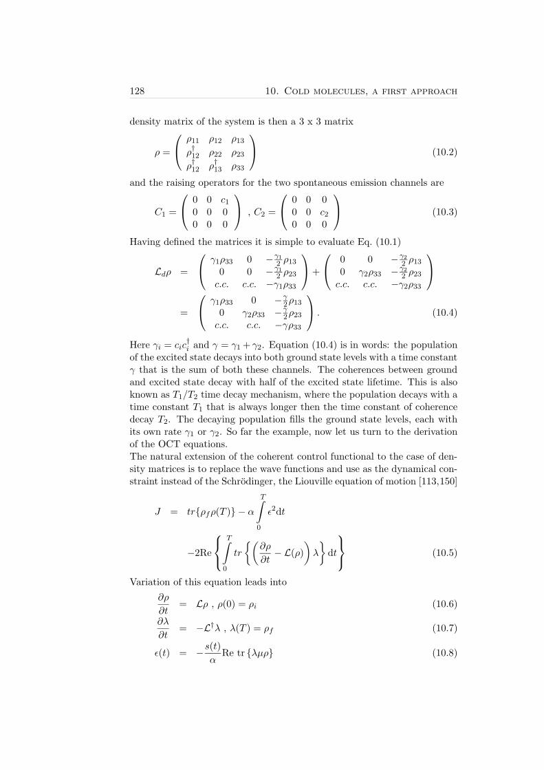
128 10. Cold molecules, a first approach
density matrix of the system is then a 3 x 3 matrix
ρ =
ρ11 ρ12 ρ13
ρ†12 ρ22 ρ23
ρ†12 ρ†13 ρ33
(10.2)
and the raising operators for the two spontaneous emission channels are
C1 =
0 0 c10 0 00 0 0
, C2 =
0 0 00 0 c20 0 0
(10.3)
Having defined the matrices it is simple to evaluate Eq. (10.1)
Ldρ =
γ1ρ33 0 −γ12 ρ13
0 0 −γ12 ρ23
c.c. c.c. −γ1ρ33
+
0 0 −γ22 ρ13
0 γ2ρ33 −γ22 ρ23
c.c. c.c. −γ2ρ33
=
γ1ρ33 0 −γ2ρ13
0 γ2ρ33 −γ2ρ23
c.c. c.c. −γρ33
. (10.4)
Here γi = cic†i and γ = γ1 + γ2. Equation (10.4) is in words: the population
of the excited state decays into both ground state levels with a time constantγ that is the sum of both these channels. The coherences between groundand excited state decay with half of the excited state lifetime. This is alsoknown as T1/T2 time decay mechanism, where the population decays with atime constant T1 that is always longer then the time constant of coherencedecay T2. The decaying population fills the ground state levels, each withits own rate γ1 or γ2. So far the example, now let us turn to the derivationof the OCT equations.The natural extension of the coherent control functional to the case of den-sity matrices is to replace the wave functions and use as the dynamical con-straint instead of the Schrodinger, the Liouville equation of motion [113,150]
J = trρfρ(T ) − αT∫
0
ε2dt
−2Re
T∫
0
tr
(∂ρ
∂t− L(ρ)
)
λ
dt
(10.5)
Variation of this equation leads into
∂ρ
∂t= Lρ , ρ(0) = ρi (10.6)
∂λ
∂t= −L†λ , λ(T ) = ρf (10.7)
ε(t) = −s(t)α
Re tr λµρ (10.8)

10. Cold molecules, a first approach 129
Note that the generalization of the overlap for matrices is the trace operationtr . The target state at final time T is ρf . The dipole matrix is µ and λ isthe conjugate density matrix (Lagrange multiplier) introduced to fulfill thedynamical constraint at all times. While the density matrix was defined tofulfill the Liouville equation with a Liouvillian L = −i[H, ρ] + Ld includingdissipation, λ fulfills a different equation that corresponds to a backward intime propagation. Inserting the explicit expression for the conjugate of Linto Eq. (10.7) one obtains
∂tλ = +i[H, ρ]−(∑
i
C†i λCi −
1
2
[
C†iCi, λ
]
+
)
. (10.9)
The signs are reversed and the role of Ci and C†i in the first summand
interchanges due to conjugation. Evaluating the dissipative part for thepreviously introduced three level system illustrates this difference
Ldλ =
0 0 −γ2λ13
0 0 −γ2λ23
c.c. c.c. −γλ33 + γ1λ11 + γ2λ22
. (10.10)
This set of equations is again solved iteratively using the Krotov or modifiedKrotov method [150] as described already in section 5.1. In contrast to thewave function analog of Eq. (10.8) here the coherences play a central rolein shaping the optimal field as will be discussed in detail in the followingsection, where the optimal control equations based on density matrices willbe applied to optimize STIRAP sequences.In this chapter the Arnoldi method [153], which is a generalization of theshort-iterative-Lanczos algorithm to complex asymmetric Liouville opera-tors, was used to propagate in time the Liouville equation with dissipation.However there exist further schemes like split-operator with a symmetrizeddissipative part to conserve the norm [154], and two further polynomialmethods the Newton and Faber [155,156] approximation. An efficient prop-agation scheme that uses a wave packet approach to the Liouville-von Neu-mann equation for dissipative systems [157] could not be used since the initialstate considered is thermal and therefore an incoherent superposition.
10.1 Simple example: STIRAP an optimal controlsolution
STIRAP [136] is the optimal solution for coherent transfer between twostates via a decaying excited state. No population is lost during the transferaffected by dissipation on the same timescale, since the population is trans-ferred adiabatically via a dressed state that is a superposition of initial and

130 10. Cold molecules, a first approach
target state with no decaying state component. The superposition state isgenerated by a counterintuitive ordering of frequencies, the dump precedingthe pump pulse. It is expected, as will be proven in a moment, that theseoptimal solutions do not come out of the closed form, rapidly convergentoptimal control theory (OCT) formulation based on mere population evo-lution [27, 29]. Therefore there have been several attempts to devise otheroptimal control schemes also based on a wave packet description, like lo-cal control [112, 158] or gradient-type [32, 159] optimizations to naturallyinclude these counterintuitive solutions. These methods however lack theglobal search capability of the closed form expressions and are therefore in-ferior. This section shall illustrate that it is not necessary to resort to theseless optimal schemes, since OCT based on density matrices as written downin Eqs. (10.6-10.8) naturally includes the STIRAP solutions. This is dueto the fact, that the electric field is build from the coherences as well aspopulations in the system [see Eq. (10.8)]. In contrast, the wave functionOCT is not able to optimize STIRAP due to Eq. 5.10. This can be provenby contradiction. Without loss of generality let us assume the typical Λsystem with ground state levels |g1〉 and |g2〉 and decaying excited statelevel |e〉. Let us assume further that wave packet OCT has converged intothe counterintuitive STIRAP sequence. Convergence means that ψ and theLagrange multiplier λ proceed along the same path in phase space. Sincethe field is a STIRAP sequence the population in the excited state λe andψe is zero. Hence using Eq. (5.10) one obtains for the Λ system
ε(t) = −s(t)α
Im〈λg1|µ|ψe〉+ 〈λg2|µ|ψe〉+ c.c = 0! (10.11)
and the field is for all times zero, which is in contradiction to the assump-tion, that it is a STIRAP field.If instead of the Krotov way of updating the field as assumed in Eq. (10.11),the modified Krotov is used the statement of the above proof is less strict. Inthis case it states that the correction to the field vanishes ones the STIRAPfield is found. This proof was also checked numerically. The wave packetOCT in combination with Krotov is incapable of finding a STIRAP solu-tion, even if the initial guess was already counterintuitive. Instead aftersome iterations the zero field solution emerged. However using the modifiedKrotov it was possible to optimize STIRAP, but it took several thousanditerations, since the corrections are proportional to the square of the pop-ulations and the populations of the decaying states being already small forcounterintuitive pulse sequences close to STIRAP. A consequence of slowconvergence is that the initial guess has to be already close to the optimalSTIRAP solution.The above mentioned proof breaks down for density matrix OCT, sinceclearly in the equation that predicts the electric field for the next iterationboth populations and coherences enter. In STIRAP the populations for

10. Cold molecules, a first approach 131
the decaying states vanish, however not their coherences to the other levels.This is the key reason, why density matrix OCT includes counterintuitivesolutions efficiently in its solutions space. To illustrate this, optimizationson the Λ system will be performed in the following.In the density matrix formalism the current state of the Λ system is de-scribed by 3×3 matrix. A decay using wave functions can only be describedby an imaginary term iγ, which physically is a decay into nowhere. In theLindblad formulation decays into nowhere do not exist and each decay chan-nel must have a source and a sink. Hence the Λ system must be extended bya fourth, dark state |d〉. It merely serves as sink of the population decayingfrom the excited state |e〉 and has no dipole coupling to any other state.This darkness of the state just defines that the population that decayed islost to the laser transfer. A spontaneous decay back into the ground statelevels would also have been a possibility, but it is not the exact analog of theiγ decay. The respective energies in wave numbers are Eg1 = 0, Ee = 10973cm−1, Eg2 = 2195 cm−1. Due to the further dark state the density matrixis 4×4
ρ =
|g1〉〈g1| |g1〉〈g2| |g1〉〈d| |g1〉〈e|c.c |g2〉〈g2| |g2〉〈d| |g2〉〈e|c.c. c.c. |d〉〈d| |d〉〈e|c.c. c.c. c.c |e〉〈e|
, (10.12)
and the lowering operator describing spontaneous emission is
C =
0 0 0 00 0 0 00 0 0 Γ0 0 0 0
. (10.13)
The consideration of coherences together with the Λ system extended by adark state are the essentials to obtain STIRAP-type solutions. Fig. 10.1(a)displays the short-time Fourier transform (STFT) of the initial guess pulse.It was designed to have already the counterintuitive ordering of frequencies.However as the evolution of the populations in the system shows the upperstate is populated to a considerable amount [see Fig. 10.2(a)]. This means,in the case spontaneous emission is turned on (Γ−2 ≈ 150 fs), the targetstate is only poorly reached at final time [Fig. 10.2(c)]. The optimal controlpulse found in the case of this decay strength (Γ−2 ≈ 150 fs) is shown inFig. 10.1(b). This pulse improves considerable on the amount of populationtransferred to the target state [see Fig. 10.2(d)]. That this pulse is indeednearly perfectly a STIRAP pulse can be seen in the propagation withoutdissipation (Γ = 0), where at final time a population of less than 2% accu-mulates in the excited state [Fig. 10.2(b)]. Due to the decay of coherences(T2 = 2T1) in addition to population decay the transfer can not be complete.

132 10. Cold molecules, a first approach
Figure 10.1: (a) Initial guess pulse. (b) Optimal pulse for Γ−2 ≈150 fs. (c)Optimal pulse for Γ−2 ≈50 fs.
In the case of even stronger decay (Γ−2 ≈50 fs) leading to even shorter T1
and T2 times, the optimal pulse of Fig. 10.1(c) generalizes STIRAP. Insteadof only two center frequencies a comb of frequencies emerges to cope with thestronger coherence (or polarization) decay. The extra frequencies serve tobuild up further coherent bridges between the initial and final state, increas-ing thereby the overall coherence, in order to compensate for the strongerT2 decay.After this simple illustrative example density matrix OCT is applied in thenext section to the problem of molecular cooling as pioneered by Tannorand coworkers [150,160].
10.2 Molecular cooling with shaped laser fields
Before presenting the results on molecular cooling a definition of coolingmust be given. This introduction is based on a paper by D. Tannor [161].The coolness of a sample is best defined by its purity, that is tr
ρ2, which is
the expectation value of ρ itself. The adequacy of this measure is due to thefact that tr
ρ2=∫ ∫
dq dp ρ2(q, p), the phase space density [160]. Thatmeans every pure ensemble ρ = |ψ〉〈ψ| is absolutely cool, i.e. a coherent su-perposition or wave packet is absolutely cool. In essence it is important howthe initial statistical mixture is transformed into a pure state. If this is doneby just stripping away population, then tr
ρ2is constant1), that means
phase-space density is not increased and the sample is not cooler then it wasinitially in the sense of having approached Bose condensation. Now it is wellknown that the coldest gas in the universe, the Bose-Einstein-Condensate,
1)However in this process the von Neumann entropy decreases.

10. Cold molecules, a first approach 133
0.001
0.01
0.1
1
0 1 20.001
0.01
0.1
1
0 1 2time [ ps ]
popu
latio
n
(a) (b)
(c) (d)
Figure 10.2: State populations of the extended Λ system: initial (filled dots), tar-get (hollow dots), excited decaying (straight line) and dark/sink (hollow squares).(a) Evolution of population under influence of initial guess pulse. Γ = 0. (b) Evo-lution of population under influence of optimal pulse. Γ = 0. (c) Same as (a) butΓ−2 ≈150 fs. (d) Same as (b) but Γ−2 ≈ 150 fs.
can only be reached by increasing phase-space density. The central questionof cooling is then: How can a statistical ensemble be transformed into a pureone, increasing at the same time the phase-space density? Atom physics tellsus, that lasers can be used to accomplish that task. At first, cooling usingelectric fields seems to be a contradiction, since it is impossible to increasephase space density with time-dependent terms in the Hamiltonian as wasshown in a paper from Ketterle and Pritchard [162]. One essential partof this paper can be summarized in a single equation, that calculates thechange in purity achieved through an electric field [161]
d
dttrρ2= 2tr ρρ = 2tr ρ(−i)[H, ρ] = 0 ! (10.14)
This equation states, that no cooling can be achieved, due to the permuta-tion invariance of the trace tr ρHρ− ρρH = tr ρρH − ρρH = 0. Theessential key ingredient missing is dissipation, i.e. in the form of spontaneousemission. Interestingly however dissipation does not lead automatically tocooling, but can also lead to heating of the ensemble, depending on theinitial population distribution [161]. As an example take a pure ensembleof two-level atoms, where the population of all atoms is initially in the de-caying excited state. That means initially the ensemble is absolutely cool

134 10. Cold molecules, a first approach
since it is in a pure state. As time progresses decay heats the ensemble sincethe atoms will then be in an incoherent superposition: some atoms beingalready in the ground and other still in the excited state.Interactions with the externally controllable laser field do not change the
1 0.5 0.1
α
β
Figure 10.3: Schematic showing isopurity surfaces and the control possible withHamiltonian (gray arrow) and dissipative operations (black arrow). The multidi-mensional space is spanned by sets of quantum numbers α and β the purity dependsupon.
purity and therefore move the ensemble around on an isopurity surface inphase space2), while dissipation essentially uncontrollable is the only mecha-nism connecting the isopurity surfaces. A schematic showing these relationsis shown in Fig. 10.3, where the black arrow shows a dissipative and thegray arrow an Hamitonian action. Cooling is therefore an interplay of acontrollable part: the laser field and an uncontrollable part: dissipation.Alternately cooling can be viewed as a two-step process, since d/dt(tr
ρ2)
does not depend on the electric field, however the second derivative of ρdoes. Molecular cooling is then in a first time step an uncontrollable slowdissipative action and in a second step a purely Hamiltonian fast action.In atoms it is not important that dissipation is uncontrollable since closedtransitions exist, that means dissipation takes the system on the same wayback as it was excited. Even in Raman cooling the dissipation is not closedbut strongly controlled, since the spontaneous emission is most favorable inthe case of no velocity change. In molecules however dissipation takes theexcited population back not only to the levels that where initially populated,but also to many others, leading essentially with each excitation to an everincreasing population spread over the molecule.Bartana, Tannor and Kosloff proposed to solve this intricate problem ofmolecular cooling by using density matrix OCT [150]. They decomposedthe problem into cooling of the vibrational and afterwards of the rotational
2)a surface where the purity is constant

10. Cold molecules, a first approach 135
manifold. The model for vibrational cooling was a molecule consisting oftwo electronic potentials. They found the following cooling mechanism: theoptimal laser field does not interact with the target level in the ground po-tential (“dark state”), while it pumps the population in all other groundstate levels to the excited state were it decays back into all ground statelevels, including the dark state. After several vibrational periods of themolecule the induced cycling of population (excitation and decay) finallyfills the dark state and the molecule ends in a pure state. Rotational coolingwas studied in a truncated rotational manifold. The optimal cooling mech-anism found in this case makes use of an alternation between right and leftcircularly polarized light [163].In both cases the optimal pulses emerged automatically from the densitymatrix OCT [see Eq. (10.5)]. Note that the goal is to make the purity ofthe molecule equal to 1, however no optimal control scheme can be derivedif tr
ρ2is defined to be the target in the functional J . Therefore one has
to use the functional of Eq. (10.5) and define as target state some arbitrarypure state. As a consequence the optimal pulse shape and possibly the finalpurity can depend on the chosen target state. However from controllabilityarguments [164, 165] such a dependence on the target state is not expectedto occur, since two different density matrices with the same purity can betransformed into one another by an Hamiltonian operation. This mere pop-ulation transfer takes place fast compared to the dissipation. Thereforehaving reached some final value for the purity, transformation between theclass of ensembles with the same purity but different population distributionamong the levels in the system is possible.The following numerical results however contradict this mathematical ar-gumentation. Pure vibrational cooling is studied in a simplified molecularsystem consisting of an excited set of five vibrational levels that decay intofive other vibrational ground state levels. The energy spacings are ∆λg ≈ 92cm−1 (360 fs), ∆λe ≈ 67 cm−1 (520 fs) and correspond to the values inthe potassium dimer. A rotating-wave approximation is performed and thedipole moments between excited and ground state levels were calculatedby taking into account the r-dependent K2 dipole moments. Spontaneousemission occurs between all excited and all ground state levels and is notsubject to any selection rule. It was taken in the Lindblad form, where thei-th lowering operator is ΓiCi. The decay constant Γ−2
i ≈ 2.5 ps, the finaltime T = 28 ps and a time step 2.3 fs were chosen. The initial state wastaken to be the 10×10 matrix with all zeroes except to the first five diagonalelements, that were set to 0.2. This is, the initial population is distributedequally over the five ground state levels. The STFT of the optimal pulses areshown in Fig. 10.4 for two different target states: v′′ = 0 [10.4(a)] and v′′ =2 [10.4(b)]. The purity as a function of time for these two cases is shown inFig. 10.5. Clearly not only do the pulse shapes differ considerably, but alsothe purity at the end depends strongly on the final pure state. As discussed

136 10. Cold molecules, a first approach
Figure 10.4: STFT of optimal pulses that cool an initial population distributedevenly over ground state levels. The pure target state was chosen to be v′′ = 0 (a)and v′′ = 2 (b).
earlier this result is mathematically not expected, since if it is possible toreach an ensemble purity of 0.7 with the population mostly in v′′ = 0 [seeFig.10.5 line], why should it not be possible to concentrate the populationin v′′ = 2 without loosing purity, just by an Hamiltonian operation?! Theonly explanation to this discrepancy is to assume that the OCT scheme doesnot find the most optimal solution or that the solution is not allowed dueto the constraint on the pulse energy or shape s(t). The optimal laser fieldsfrom chapter 8 connecting two pure states are in this mathematical sensealso imperfect, since their yield is less than 100%. From the mathematicalpoint of view both states are pure and therefore there must exist an Hamil-tonian operation that fulfills the task with unit efficiency independent of theinitial/final state pair.Even more surprising is that the purity at earlier times reaches a maximumand falls off again on timescales much faster than dissipation before final time[see Fig. 10.5]. A purity change with a timescale faster than dissipation (2.5ps) should be impossible, since the fast acting Hamiltonian operations arepurity conserving.The optimal pulses of Fig. 10.4 have to increase the purity and steer thepopulation into some final density matrix. Instead by defining the finalstate to have the same diagonal elements, but the necessary coherences onthe off-diagonal to be pure it is possible to eliminate the second, populationtransfer step from the pulses. The target state with tr
ρ2having the same

10. Cold molecules, a first approach 137
Figure 10.5: The evolution of purity in time for the two pulses of Fig. 10.4. Linecorresponds to 10.4(a) and hollow dots to 10.4(b).
diagonal elements as the initial matrix is the density matrix
ρf =
0.2 if i, j = 1 . . . 50.0 else
(10.15)
For this calculation the time step was reduced to dt = 1.16 fs. The optimalpulse now resulting is shown in Fig. 10.6(c) and the purity at final time T= 7 ps is 80% [see Fig. 10.7 line], that is a higher purity than was achievedfor the two previous optimizations, that used a specific eigenstate as finalstate. In order to study the effect of the decay rate on the final purity adecay rate five times slower, that is Γ−2
i ≈12.5 ps, is studied. Clearly for thissystem the lower spontaneous emission rate will lead to slower cooling rateand a smaller final purity. What happens however if not all, but only onedissipative channel is increased by a factor of five? Calculations, where onlythe v′ = 0 Ã v′′ = 0 spontaneous emission channel is increased by a factorof five lead to the optimal field of Fig. 10.6(a) and to a purity versus time asshown in Fig. 10.7. Increasing more dissipative channels (all five connectingto v′′ = 0) by a factor of five results in the pulse of Fig. 10.6(b) and the purityin Fig. 10.7. A comparison of all the tailored fields in Fig. 10.6 clearly showsthat the optimal pulse adapts to the spontaneous emission characteristics.Moreover Fig. 10.7 shows that an increase of only part of the channels canlead to an increased purity at final time. This increase of dissipation canbe easily done numerically, however it is not clear what physical mechanismcould be used to achieve such an increase. One possibility is to place themolecule inside a lossy cavity. It is known that the cavity changes thevacuum field density of modes increasing or decreasing thereby spontaneousemission [166–169]. The field modes of the cavity can be controlled bythe curvature of the cavity mirrors [170]. The effect of the cavity can be

138 10. Cold molecules, a first approach
Figure 10.6: STFT of cooling pulse for different dissipation. (a) Γ−2i ≈12.5 ps
but dissipative channel v′ = 0 Ã v′′ = 0 increased by factor of five. (b) Γ−2i ≈12.5
ps but all dissipative channels ending in v′ = 0 enhanced by factor of five. (c) Alldissipative channels with Γ−2
i ≈2.5 ps.
expressed by a simple formula [166]
η =3Qλ3
4π2V(10.16)
where η is the ratio of spontaneous emission to free-space emission rate, Qis the cavity quality factor, λ the transition wavelength and V the modevolume. In experiments η ≈ 3 . . . 5 can be realized. In a cavity a combof transversal modes can be created, that depend on the curvature of themirrors. Molecular cooling in a cavity was proposed by Vuletic et. al. [166],where the cavity mode is blue shifted with respect to all molecular transition,so that in a Raman scattering event the loss of energy is enhanced. Oncethe molecule is translationally cold the internal degrees of freedom couldperhaps be cooled by matching the cavity modes with the band heads of ro-vibronic transitions. This possibility is the topic of further research as wellas obtaining simpler cooling pulses, since electric fields like the one shownin Fig. 10.8 are not yet realizable.

Figure 10.7: Purity evolution for the three pulses of Fig. 10.6. 10.6(a) correspondsto filled, 10.6(b) to the hollow dots and 10.6(c) to the line.
Figure 10.8: (a) Electric field in rotating wave approximation of the pulse inFig. 10.6(c). (b) The spectrum of this pulse.
139


Chapter 11
Cold molecules, a secondapproach
11.1 Bose-Einstein-Condensates and Feshbach res-onances
The Bose-Einstein-Condensate (BEC). The many-body Hamiltoniandescribing N interacting bosons confined by a trapping potential Vtrap isgiven, in second quantization, by
H =
∫
d3r
[
− ~2
2m∇2 + Vtrap(r)
]
ψ†(r)
+1
2
∫ ∫
d3r d3r′ψ†(r)ψ†(r′)V (r− r′)ψ(r′)ψ(r) (11.1)
where ψ(r) and ψ†(r) are the boson field operators that annihilate andcreate a particle at the position r, respectively, and V (r− r′) is the two-body interatomic potential. The dynamics of the condensate are predictedby the Heisenberg equation with the many-body Hamiltonian Eq. (11.1):
i~∂tψ(r, t) =[
ψ,H]
(11.2)
This equation is solved to first order with the Ansatz ψ(r, t) = φ(r, t) +ψ′(r, t), where essentially the condensate contribution φ is separated outfrom the bosonic field operator. Here φ(r, t) is a complex function definedas the expectation value of the field operator: φ(r, t) =< ψ(r, t) >. Itsmodulus specifies the condensate density through n(r, t) = |φ(r, t)|2. Thefunction φ(r, t) is a classical field having the meaning of an order parameterand is often called the “wave function of the condensate”. In a dilute and ul-tracold gas only binary collisions in s-wave (l=0) geometry can occur, wherea single parameter, the s-wave scattering length a suffices to describe these
141

142 11. Cold molecules, a second approach
interactions. All the details of the two-body potential are subsumed in thescattering length and therefore two potentials resulting in the same scatter-ing length are not distinguishable. This allows one to replace V (r− r′) withan effective interaction
V (r− r′) =4π~2a
mδ(r− r′). (11.3)
Inserting this potential into Eq. (11.2) together with the replacement ψ withφ yields the Gross-Pitaevskii (GP) equation for the order parameter:
i~∂tφ(r, t) =(
−~2∇2
2m+ Vtrap + U0|φ(r, t)|2
)
φ(r, t) (11.4)
with
U0 =4π~2a
m. (11.5)
The validity of the GP equation is based on the condition that the s-wavescattering length be much smaller than the average distance between atomsand that the number of atoms in the condensate be much larger than 1. Themean-field or self-energy term U0|φ|2 results from the above delta-functionpseudopotential and shows that the interaction energy in a cloud of atomsis proportional to the density and the scattering length. The sign of thescattering length indicates whether the atomic interaction is effectively re-pulsive (a > 0) or attractive (a < 0). For negative a with Vtrap = 0 the GPequation does not have a stationary solution. In practice that means thecondensate collapses. With a harmonic trap potential and a < 0 the GPequation has a stable solution, but only if the mean-field energy is less thanthe spacing of the trap levels. When a = 0 the atoms do not interact andthe stationary solution equals the single-atom ground-state wave functionin the trap potential (except for normalization).
Feshbach resonances. Feshbach resonances are scattering resonancesthat arise when the total energy (internal+translational) of a pair of collidingatoms matches the energy of the quasibound two-atom state, leading toresonant formation of this state during collision. Magnetic tuning is possibleif the magnetic moments of the free and quasibound states are different. Ina time-dependent picture, the two atoms are transferred to a quasiboundstate stick together and then return to an unbound state. Such a resonancestrongly affects the scattering length (elastic channel). Near a Feshbachresonance the scattering length a varies dispersively as a function of themagnetic field B:
a = a
(
1− ∆
B −B0
)
, (11.6)

11. Cold molecules, a second approach 143
where ∆ is the width of the resonance at B = B0, and a is the scatteringlength outside the resonance. Clearly, the scattering length a covers the fullcontinuum of positive and negative values, above and below the resonance.A microscopic understanding of a Feshbach resonance can be obtained ina quantum mechanical description of interaction processes between alkaliatoms. The effective Hamiltonian describing the collisions of two ground-state alkali atoms is
H =p2
2µ+
2∑
j=1
(
V hfj + V Z
j
)
+ V c (11.7)
comprising the relative kinetic energy operator with reduced mass µ, asingle-atom hyperfine V hf
j and Zeeman term V Zj for each atom j, and a
central two-atom interaction term V c. The central interaction V c repre-sents all Coulomb interactions between the electrons and the nuclei of bothatoms. It depends only on the quantum number S associated with the mag-nitude of the total electron spin ~S = ~s1 + ~s2, which can be 0 or 1 for alkaliatoms, and the internuclear distance r:
V c = VS(r)PS + VT (r)PT (11.8)
with PS and PT the projection on the singlet (S = 0) and triplet (S = 1)subspaces. The potentials VS and VT are the Born-Oppenheimer molecularpotential curves connected to the 32S1/2 + 32S1/2 separated-atom limit;in spectroscopic notation the corresponding molecular electronic states areX1Σ+
g and a3Σ+u . At large separations (r > 16 a0 to 19 a0, depending on
the atomic species), the central potentials may be written as
VS,T (r) = −C6
r6− C8
r8− C10
r10± VE(r). (11.9)
The first term represents the van der Waals interaction. It is followed bythe next two terms in an electric multipole expansion of the Coulomb in-teractions between the charge distributions of the two colliding atoms: thedipole-quadrupole and quadrupole-quadrupole interactions. The differentpermutation symmetries of the molecular electronic wave functions ψS andψT are responsible for the exchange interaction energy VE(r).The hyperfine terms are given by
V hfj =
ahfj~2~sj ·~ij , (11.10)
where ~sj and ~ij are the electron and nuclear spin operators of atom j and
ahfj a constant related to the hyperfine splitting. Alkali atoms have only one
valence electron, therefore s1 = s2 = 12 . Under the influence of the hyperfine
interaction the electronic ground state (3S for Na) splits into two new levels,with the total spin vector ~f =~i+ ~s = i± 1
2 (see Fig. 11.1 at B = 0).

Figure 11.1: Hyperfine states of sodium |f,mf 〉. Shown is the energy dependenceof these states in an external magnetic field B (Zeeman dependence). The relativeorientation of the nuclear and electron spin is depicted by the large and small ballsat the right. ~f = ~i + ~s is the orientation dependent total spin vector of nuclear iplus valence electron spin s. The projection of ~f on the quantization axis is givenby mf .
144

11. Cold molecules, a second approach 145
The Zeeman interaction accounts for the external magnetic field. Choos-ing the z-axis of the laboratory frame along the magnetic field ~B = B~ez,they have the form
V Zj = (γeszj − γN izj)B. (11.11)
Asymptotically, where the two-atom interaction V c can be neglected, thesystem is described by separate atoms, each in an eigenstate of its ownhyperfine and Zeeman operators. These are the magnetic-field dependenthyperfine states |f,mf 〉 shown in Fig. 11.1. The kind of states with increas-ing (decreasing) energy with increasing magnetic field are called low-field(high-field) seeking states, respectively. While low-field seeking states can betrapped in a magnetic-field minimum, a BEC in a high-field seeking state canonly be trapped by all optical means. The differences in field dependence be-tween the hyperfine states are responsible for Feshbach resonances [171,172].The details of a cold collision enhanced by a Feshbach resonance is shownschematically in Fig. 11.2. The colliding atoms are assumed to be in the
E
|f1,m
f1>
|f2,m
f2>α
E
|f1,m
f1>
|f2,m
f2>
γ0
(a) (b) (c)
E
|f1,m
f1>
|f2,m
f2>
Figure 11.2: Shown are the collisional potential energy surfaces of two hyperfinestates |f1,mf1〉 and |f2,mf2〉. The atoms in the BEC are assumed to be in thehyperfine state |f1,mf1〉 possessing a kinetic energy Ekin. (a) Off resonance situa-tion. The colliding atoms can not penetrate the quantum reflection region. (b) Theexternal magnetic field is tuned in resonance with the Feshbach resonance. Spinflip tunneling is now enhanced due to the bound state resonance condition. Thetunneling rate is α. (c) The quasibound state has a local lifetime. If during thistime the external field changed, the dissociating atoms acquire additional kineticenergy leading to a trap loss γ0.
lower energetic hyperfine state |f1,mf1〉. As they approach each other theyenter a small range near the beginning of the long-range region (r ≈ 20a0), where the exchange interaction VE is of the same order of magnitudeas the hyperfine-Zeeman energies. This is a crucial region because in anexternal field the hyperfine induced spin flip of the one atom in presence ofthe other can bind the interacting atoms by bringing them to a hyperfinestate |f2,mf2〉 with a higher threshold energy. Normally no bound state ofthe |f2,mf2〉 scattering potential coincides in energy with the total energyof the colliding atoms and the atoms get reflected back [see Fig. 11.2(a)].If the Zeeman dependence of the two hyperfine states is different it is pos-sible to tune a bound state of the |f2,mf2〉 scattering potential exactly in

146 11. Cold molecules, a second approach
resonance with the collision threshold. Now the atoms can tunnel into thequasibound molecular state, where they are at small interatomic separationsand form a molecular condensate [Fig. 11.2(b)]. After some local lifetimeof the resonance the two atoms dissociate again. If during this lifetime themagnetic field is decreased and the |f2,mf2〉 hyperfine state is high-fieldseeking the quasibound state will have risen in energy. As a consequencethe dissociating atoms will have acquired an additional kinetic energy andwill be lost from the trap [173]. This decay is characterized by the constantγ0 [ Fig. 11.2(c)]. Note that this decay does not occur if the magnetic fieldwas instead increased.In the many body Hamiltonian, the spin flips to quasibound states are de-scribed by [174]
HFR = α
∫
d3rψ†m(r)ψa(r)ψa(r) + c.c., (11.12)
where ψm, ψ†m (ψa, ψ
†a) are the annihilation and creation field operators
of the molecules (atoms). The α parameter in Eq. (11.12) is the transi-tion matrix element proportional to the overlap of the molecular continuumand bound state wave functions. The expectation value of the Heisenbergequations for atoms and molecules gives the equation of motion for the con-densate fields φm =< ψm > and φa =< ψa >:
i~φm =
[
−~2∇2
4M+ Em + λmnm + λna
]
φm + αφ2a
i~φa =
[
−~2∇2
2M+ U0na + λnm
]
φa + 2αφ?aφm, (11.13)
where M denotes the mass of a single atom, nm and na represent the con-densate densities, nm = |φm|2 and na = |φa|2, and λm, U0 and λ representthe strength of the molecule-molecule, atom-atom and molecule-atom in-teractions. The α-terms that couple the equations describe the tunnellingof pairs of atoms between φm and φa-fields. Eq. (11.13) replaces the usualsingle condensate Gross-Pitaevskii equation (11.4).The following sections study the stabilization of the naturally forming mole-cular condensate during a Feshbach resonance via optimally shaped Ramanfields in the nanosecond and femtosecond regime.
11.2 Optimal conversion of an atomic to a mole-cular BEC
Cold molecules have been produced and detected through photoassocia-tion [175–177] of laser-cooled atoms, where the molecules are formed in-coherently in many different ro-vibrational levels and have a relatively large

11. Cold molecules, a second approach 147
energy spread of 100 µK. However it is also possible to form moleculesby a stimulated Raman transition from a freely moving pair of condensateatoms [138, 140, 142, 178, 179]. Note that the energy and impulse is con-served, since the Raman light fields can be applied counter propagating andthe energy released during molecule formation is carried away by the lightfields. The free to bound photoassociation process is not very efficient dueto poor Franck-Condon overlap of the relatively short distances of atoms inthe molecule and the diffuse interatomic distances of a pair of interactingtrapped atoms. The free atoms can not penetrate small distances due to thequantum reflection region [180], which is opaque for atoms moving at 1 nKkinetic energies. A further complication is that the Franck Condon factorsare best for bound states near the dissociation limit of the excited electronicstates, and thus the pump laser tuned to this wavelength will unavoidablyexcite the nearby atomic transition.A more promising scheme is the partial conversion of an atomic to a diatomicmolecular condensate via a stimulated Raman transition, enhanced by atime-dependent magnetic field that sweeps over a Feshbach resonance [143].Here a dramatic increase of the free-bound transition probability by sevenorders of magnitude can be achieved, since the colliding atoms can pene-trate to the short distance range. The conversion rate depends criticallyon the Raman fields used, which were hand-optimized guided by physicalintuition [143]. In this thesis the required fields are calculated by optimalcontrol theory [27, 29], which is very successful in finding solutions close toglobal optimum. In order to do so, the well known optimal control equationshad to be extended to the case of nonlinearities in the dynamical equation.The BEC to M-BEC conversion is moreover a challenge, because it is partof the important class of problems in which the coherent transfer is affectedby dissipation on the same timescale.
11.2.1 Nonlinearity
In order to make theoretical predictions useful for experiment, the theory willbe specialized to a recent experiment on Feshbach resonances carried out atMIT [181,182]. Here a BEC in the high-field seeking state |f = 1,mf = +1〉,for which two Feshbach resonances at realizable magnetic field strengths of853 G and 907 G were theoretically predicted [183], is trapped by all op-tical means. Then by sweeping the external magnetic field with a rate of0.31 10−2G/µs over the 853 G resonance 60% quasibound molecules couldbe created. The parameters of the Feshbach resonance and the Na BECare summarized in Table 11.1. The atomic condensate (of Na atoms as anexample) is described by the field φa(~x, t), the atom pairs in their inter-mediate Feshbach 32S1/2 + 32S1/2 quasibound state as a molecular Bose-Einstein condensate with order parameter φ1(~x, t). Two further condensatecomponents are considered: the molecules in the intermediate electronically

148 11. Cold molecules, a second approach
Table 11.1: The parameters of the calculation.
a 3.3 nm γ0 5.3 µK∆ 0.0091 G γsp 6 107 · ~ s−1
n 5.2 1014 cm−3 m 0.38175 10−25
B ± 0.31 10−2 G/µs α√
2 · 10−16~γ0/8U0 4π~2a/m ∆µ 2α2/(U0∆)
e1 B ·∆µ
excited 32S1/2 + 32P1/2 bound state with a bound state energy of -1346cm−1 (0−g symmetry (J, I,MI) = (2, 3,+1)) of the coherent Raman transi-tion and the molecules in the final state, described by φ2(~x, t) and φ3(~x, t)respectively. The final internal state associated with φ3(~x, t) is chosen to bethe ro-vibronic ground state of the molecule in the a3Σ+
u triplet potentialwith spin structure (S,MS , I,MI) = (1,+1,3,+1). The amplitudes of thecoherent fields are assumed uniform φj =
√nj exp(iΘj) and the interaction
with the light fields with center frequencies ω1 and ω2 is taken in a rotating-wave approximation. The coupled Gross-Pitaevskii equations of Eq. (11.13)describing the evolution of a mixed atomic/molecular BEC at a Feshbachresonance had to be extended to further include the influence of the Ramanpulse pair [143]:
iφa = U0|φa|2φa + 2αφ?aφ1
iφ1 =
(
E1 −i
2γ0
)
φ1 + αφ2a +
1
2µ1εL1φ2
iφ2 =
(
E2 −i
2γsp − ωL1
)
φ2 +1
2µ1εL1φ1 (11.14)
+1
2µ2εL2φ3
iφ3 = (E3 − ωL1 + ωL2)φ3 +1
2µ2εL2φ2
The system described by these equations is essentially a Λ-type molecularsystem, coupled to a source of atoms via tunnelling. U0 is the off-resonantstrength of the condensate self-energy, α the rate constant of atom to quasi-bound molecule conversion. The energy of the quasibound state E1− i
2γ0 isassumed complex, since it can dissociate into atoms leaving the trap when-ever the energy E1 is positive (see section 11.1). That means that the decayis only nonzero after (before) crossing the resonance for a positive (negative)magnetic field sweep, respectively. The real part E1 undergoes a Zeemanshift varying linearly in time E1 = Bt and is defined to cross the resonancevalue shifted to 0 at time 0, at which instant the φ1 to φ2 conversion ismost efficient. E2 − i
2γsp is the complex excited state energy with γsp the

11. Cold molecules, a second approach 149
α
γ0
γsp
ΩL2
ΩL1
BEC
M-BEC
φa
φ1
φ2
φ3
Figure 11.3: Schematic of the BEC to M-BEC conversion scheme using nanosec-ond Raman pulses with Rabi frequencies ΩL1 and ΩL2. Indicated are the tripletpotential a3Σ+
u and the excited potential of O−g symmetry. The colliding atomsof the BEC are described by the field φa, the formed quasibound state by φ1, thebound level in the excited potential by φ2 and finally the target level in the groundstate potential by φ3. The decay due to spontaneous emission is γsp and the decayof the quasibound state due to dissociation and trap loss is γ0.
spontaneous decay width and E3 the energy of the final bound molecularstate. For a more detailed description see Ref. [143]. Included in this modelis the boson stimulation of the free to bound transition [142] and also thechange of self-energy of the condensate due to reduction of the atomic BECcomponent during the conversion process. Not included is the effect of atom-molecule and molecule-molecule self-energy terms [see Eq. (11.13)], since noaccurate experimental or theoretical information on the relevant ultracoldcollisions is presently available.The aim is to find pulses εL1 and εL2 that take the initial population in φa(atomic BEC) completely over to φ3 (stable molecular BEC). Starting pointis the formulation of a functional, that is to be varied in order to obtain the

150 11. Cold molecules, a second approach
coupled equations solved iteratively on the electric fields:
J = 〈φ3|φ(T )〉 − α1
T∫
0
ε21(t)
s(t)dt− α2
T∫
0
ε22(t)
s(t)dt
−2Re
T∫
0
〈λ(t)|∂t + iW (φ(t), t)|φ(t)〉dt
(11.15)
Here φ(t) is a vector with the four components φi(t) describing the currentstate of the mixed condensate system governed by Eq. (11.14). Again, thefirst term describes the aim, that is to maximize the overlap with the boundmolecular state at final time tf . The next two terms are used to regulate themaximal pulse energy by choosing adequately the dimensionless parametersα1, α2. The dynamics predicted by Eq. (11.14) occur on an interval of ti =-400 µs to tf = 100 µs, while the laser interaction interval was constrainedusing a shape function to [-50 µs, 50 µs]. This selection of the optimizationwindow will allow laser fields with a fwhm of several µs and not shorterthan the dynamics induced by the initial guess pulse, which consists of asequence of nanosecond pulses. In a later section the optimization windowwill be reduced to picosecond, leading then to a shaped femtosecond Ramanpulse pair.The functional becomes unconstrained due to the last term that takes intoaccount that the evolution of φ is governed by Eq. (11.14), written inthe form i∂tφ(t) = W (φ(t), t). Here W (φ(t), t) is the right hand side ofEq. (11.14) and includes all nonlinear terms. In order to express this con-straint to be fulfilled at every time step a Lagrange multiplier λ(t) is neces-sary. Variations with respect to φ, λ, ε1 and ε2 have to be calculated to findthe fields that maximize the functional. Beginning with the electric fieldsthe following two equations are obtained:
ε1(t) = −s(t)α1
µ1Im 〈λ1|φ2〉+ 〈λ2|φ1〉 (11.16)
ε2(t) = −s(t)α2
µ2Im 〈λ2|φ3〉+ 〈λ3|φ2〉 (11.17)
Variation with respect to λ leads to Eq. (11.14) with the boundary conditionat initial time φ(ti) = φ1. The φ variation leads to the following equation

11. Cold molecules, a second approach 151
of motion for λ
iλa = U0
(
2|φa|2λa + φ2aλ
?a
)
+ 2α (φ?aλ1 + φ1λ?a)
iλ1 =
(
E1 +i
2γ0
)
λ1 + 2αφaλa +1
2µ1εL1λ2
iλ2 =
(
E2 +i
2γsp − ωL1
)
λ2 +1
2µ1εL1λ1 (11.18)
+1
2µ2εL2λ3
iλ3 = (E3 − ωL1 + ωL2)λ3 +1
2µ2εL2λ2.
Due to the nonlinear nature of Eq. (11.14) the evolution of the Lagrangemultiplier λ depends on φ itself and is not independent as for the linearSchrodinger equation. The Lagrange multiplier has to fulfill the boundarycondition λi(tf ) = δi4φ4 at final time.The obtained system of four equations, where Eq. (11.14) and Eq. (11.18)depend on the fields ε1(t),ε2(t) given by Eq. (11.16) and Eq. (11.17), respec-tively, is solved as usual by iteration on the electric fields [27]. One iterationis composed of the following steps. Starting with an initial guess pulse, φ(t)is propagated from its initial value until final time is reached. These valuesof φ(t) at each point of time are stored. Then φ(tf ) is projected onto the fi-nal state φ4 and normalized to one. This vector is then used as the boundarycondition for λ at final time tf . Both electric fields at t = tf are calculatedusing Eq. (11.16) and Eq. (11.17). These field values are used in conjunctionwith the stored value of φ to calculate λ a further step backward. This isrepeated until initial time is reached. The obtained improved field is usedas initial guess in the next iteration.The proposed iteration scheme, one out of three possible in the case of thelinear Schrodinger equation, is the only one that will work, since λ canonly be propagated if φ is already known and moreover the propagation willonly be well-behaved if Eq. (11.18) is propagated backward in time, due tothe + sign of the γ0 and γsp decay terms. Numerically the propagation isperformed using a variable-order, variable-step Adams method [184]. Analternative propagator could have been the polynomial in time proposed byR. Baer [127].The optimization is not expected to work efficiently in the case of spon-taneous emission from the excited state, since the OCT is based on wavefunctions and not density matrices (see the proof in section 10.1). Thereforethe following results were obtained with γsp = 0 and only in the next sectiona density matrix based OCT for this problem will be derived.Using the Krotov method and starting with a sequence of counterintuitivepulses in analogy to Ref. [143] [Fig. 11.4(a)], which are known to be a goodinitial guess, the results of Fig. 11.4(b) are obtained for α1 = 5 · 104 and

152 11. Cold molecules, a second approach
α2 = 1 · 1010. The population induced by the initial guess evolves accordingto Fig. 11.5(a) reaching a population in the molecular BEC at final timeof 12%. The optimal pulse population dynamics are shown in Fig. 11.5(b)with a clearly improved conversion rate to the M-BEC of 42%. The optimalpulse is a µs changing field with the subpulse coupling the quasibound to ex-cited state preceding the subpulse coupling the bound to bound transition.Therefore population is slowly transferred into the excited state and there-after dumped completely again [Fig. 11.5(b)]. With γsp turned on this pulseis no more optimal, since the laser transfer occurs on the same timescale asthe decay and population will be lost.
In the following two sections the optimal control equations will be mod-ified in order to provide solutions even in the presence of dissipation. Dissi-pation is circumvented by not populating the decaying levels (section 11.2.2)or being faster than the decay mechanism by applying tailored femtosecondpulses (section 11.2.3).
0510
ε L1
0
0.05ε L2
-0.500.5
ε L1
-40 -20 0 20 40
time [ µs ]
-1e-03
0e+00
1e-03
ε L2
(a)
(b)
Figure 11.4: (a) Initial guess consisting of a STIRAP sequence of nanosecondpulses. (b) Optimal pulse.

-5 0 5
10-2
10-1
100
-40 -20 0 20 40
time [ µs ]
10-3
10-2
10-1
100
atomsquasiboundexcitedground
popu
latio
n
(a)
(b)
Figure 11.5: Atomic BEC (filled dots) and molecular BEC: quasibound (hollowdots), excited (line), ground (squares) with γsp = 0. (a) Population transfer inducedby initial guess. (b) Population transfer induced by optimal pulse.
153

154 11. Cold molecules, a second approach
11.2.2 Use of optimal nanosecond pulses
In this section the density matrix analog of the GP equations of Ref. [143] isderived to include also the evolution of the coherences in the system. This isnecessary in order to obtain optimal pulses for the real problem of BEC toM-BEC conversion in the µs regime, where dissipation of the excited stateis a central problem. This was shown already in section 10.1, where anoptimal control functional based on dissipation was capable of optimizingSTIRAP pulse sequences. In this section the density matrix formulation ofoptimal control theory is combined with the nonlinear dynamical equationof the previous subsection to provide experimentalists with highly efficientµs pulse sequences converting an atomic to a molecular BEC. The densitymatrix elements are ρa = 〈φa|ρ|φa〉, ρai = 〈φa|〈φa|ρ|φi〉 and ρij = 〈φi|ρ|φj〉with i, j = 1 . . . 3 indexing the molecular levels. Here ρai describes theformation of the molecular quasibound state from the two colliding atomsas in Eq. (11.12). Now the density matrix analog of the coupled Gross-Pitaevskii equations [ Eq. (11.14)] predict the population dynamics
iρa = 2αρa1 − c.c.iρ11 = E1ρ11 − αρa1 +ΩL1ρ12 − c.c.iρ22 = E2ρ22 − ΩL1ρ12 +ΩL2ρ23 − c.c.iρ33 = E3ρ33 − ΩL2ρ23 − c.c.
(11.19)
and the coherence dynamics
iρa1 = (E1 − 2U0ρa)ρa1 − 4αρa(ρ11 −1
4ρa) + ΩL1ρa2 (11.20)
iρa2 = (E2 − 2U0ρa)ρa2 − 4αρaρ12 +ΩL1ρa1 +ΩL2ρa3
iρa3 = (E3 − 2U0ρa)ρa3 − 4αρaρ13 +ΩL2ρa2
iρ12 = (E2 − E?1)ρ12 − αρa2 +ΩL1(ρ11 − ρ22) + ΩL2ρ13
iρ13 = (E3 − E?1)ρ13 − αρa3 − ΩL1ρ23 +ΩL2ρ12
iρ23 = (E3 − E?2)ρ23 − ΩL1ρ13 +ΩL2(ρ22 − ρ33).
Here I used the same nomenclature as in the previous section. Again the aimis to find pulses εL1 and εL2 that take the initial population in ρa (atomicBEC) completely over to ρ33 (stable molecular BEC) without populatingthe intermediate decaying excited state. Starting point is the formulationof a functional, that is to be varied in order to obtain the coupled equations

11. Cold molecules, a second approach 155
solved iteratively on the electric fields:
J = < 3|ρ(tf )|3 > −α1
tf∫
ti
ε2L1(t)dt− α2
tf∫
ti
ε2L2(t)dt
−2Re
tf∫
ti
tr [ρ(t) +W (ρ(t), t)]λ(t)dt
(11.21)
Here ρ(t) is the 4×4 matrix
ρ =
ρa ρa1 ρa2 ρa3c.c. ρ11 ρ12 ρ13
c.c. c.c. ρ22 ρ23
c.c. c.c. c.c. ρ33
(11.22)
describing the current state, including coherences, of the mixed condensatesystem governed by Eq. (11.19). The first term describes the aim, that is tomaximize the overlap with the bound molecular state at final time tf . Thenext two terms are used to regulate the maximal pulse energy by choosingadequately the parameters α1, α2. The optimization interval is [ti, tf ] andin the calculations ti = -400 µs and tf = 100 µs were chosen. Beginningwith the electric fields the following two equations are obtained:
∆εL1(t) = −µ1
α1Imρ12(λ22 − λ11) + λ12(ρ11 − ρ22)−
λ13ρ?23 − λ23ρ
?13 + λa1ρ
?a2 + λa2ρ
?a1 (11.23)
∆εL2(t) = −µ2
α2Imρ23(λ33 − λ22) + λ23(ρ22 − ρ33) +
λ12ρ?13 + λ13ρ
?12 + λa2ρ
?a3 + λa3ρ
?a2. (11.24)
Clearly these equations, that are used to predict the optimal fields in each it-eration, depend on the populations and coherences of the system. In compar-ison the equations (11.16) and (11.17), obviously lack the coherence terms.The iteration behavior using Eqs. (11.23) and (11.24) with Eqs. (11.16) and(11.17) was compared. The density matrix formulation of the GP equationsis not only a physically more complete picture, but the coherence termslead to a much faster optimization of STIRAP light fields compared to wavefunction OCT (see the proof in section 10.1).Variation with respect to λ leads to Eq. (11.19) with the boundary conditionat initial time ρ(ti) = ρa. The ρ variation leads to the following equation of

156 11. Cold molecules, a second approach
motion for λ
iλa = −2U0(ρ?a1λa1 + ρ?a2λa2 + ρ?a3λa3) +
2α[(ρa − 2ρ11)λa1 − 2ρ?12λa2 − 2ρ?13λa3]− c.c.iλ11 = E?
1λ11 − 4αρ?aλa1 +ΩL1λ12 − c.c.iλ22 = E?
2λ22 − ΩL1λ12 +ΩL2λ23 − c.c.iλ33 = E?
3λ33 − ΩL2ρ23 − c.c.iλa1 = (E?
1 − 2U0ρa)λa1 − α(λ11 − 2λa) + ΩL1λa2 (11.25)
iλa2 = (E?2 − 2U0ρa)λa2 − αλ12 +ΩL1λa1 +ΩL2λa3
iλa3 = (E?3 − 2U0ρa)λa3 − αλ13 +ΩL2λa2
iλ12 = (E?2 − E1)λ12 − 4αρaλa2 +ΩL1(λ11 − λ22) + ΩL2ρ13
iλ13 = (E?3 − E1)λ13 − 4αρaλa3 − ΩL1λ23 +ΩL2λ12
iλ23 = (E?3 − E2)λ23 − ΩL1λ13 +ΩL2(λ22 − λ33)
Due to the nonlinear nature of Eq. (11.19) the evolution of the Lagrangemultiplier λ depends on ρ itself and is not independent as for the linearSchrodinger equation. The Lagrange multiplier has to fulfill the boundarycondition λi,j(tf ) = δi4,j4 at final time. The obtained system of four equa-tions (Eq. (11.19), (11.23), (11.24), and (11.25)), where Eqs. (11.19) and(11.25) depend on the fields ε1(t),ε2(t) given by Eqs. (11.23) and (11.24),respectively, is solved by iteration on the electric field using the modifiedKrotov method, since the Krotov method always results in a zero light fieldwhen γsp is turned on. This was already proven in section 10.1. Iteration wasstopped when the yield did not increase monotonically anymore. Critical tothe iteration performance are the values of α1 and α2, which were chosen asclose as possible to their thresholds, below which convergence breaks downand strong oscillatory behavior sets in. Too high values will slow down con-vergence drastically. For the problem at hand α1 = α2 = 2 103 proved tobe the best and closest to threshold.

0
50
ε L1(t
) [ (
W/c
m2 )0.
5 ]
-10 -7.5 -5 -2.5 0 2.5 5
time [ µs ]
-50
0
50
ε L2(t
) [ (
W/c
m2 )0.
5 ]
Figure 11.6: Optimal Raman pulse pair for positive magnetic field sweep. Lightfield (εL1) coupling quasibound state with excited state and light field (εL2) inducingtransition between excited and target molecular state. As reference the initial guessRaman sequence of Ref. [143] is shown as line.
0
50
100
ε L1(t
) [ (
W/c
m2 )0.
5 ]
-10 -7.5 -5 -2.5 0 2.5 5
time [ µs ]
0
50
ε L2(t
) [ (
W/c
m2 )0.
5 ]
Figure 11.7: As Fig. 11.6 for negative magnetic field sweep.
157

158 11. Cold molecules, a second approach
The STIRAP sequence of seven consecutive equidistant pulses of Ref.[143] [Figs. 11.6 and 11.7] transfers 16% of the population into the molecu-lar BEC if a positive magnetic field sweep is applied [see Fig. 11.8(a)] and25% in conjunction with a negative sweep [see Fig. 11.8(b)].Taking this STIRAP sequence as initial guess Raman pulse into the op-
10-2
10-1
100
popu
latio
ns
atomsquasiboundexcitedground
-20 -10 0 10 20
time [ µs ]
10-2
10-1
100
popu
latio
ns
(a)
(b)
Figure 11.8: Population dynamics as induced by the STIRAP sequence of sevenpulses. (a) for positive linear magnetic field sweep. (b) for negative linear magneticfield sweep.
timal control formulation, the yield could be improved upon considerably.The resulting optimal light fields are shown in Figs. 11.6 and 11.7, for thecase of positive and negative magnetic field sweep, respectively. Under theinfluence of the pulse in Fig. 11.6 [Fig. 11.7] the population evolves accord-ing to Fig. 11.9 [Fig. 11.10]. In the upper panel the population dynamicsare depicted and in lower panel the coherences. While the population in theexcited state ρ22 is less than 1% during the transfer the coherence terms,especially the important one, ρ13, coupling the quasibound state with thetarget state, are ten times larger. These terms give important corrections tothe electric fields in each iteration via Eqs. (11.23) and (11.24), while theyare completely missing in the electric field correction equations in the wavefunction OCT.The optimal Raman pulses of Figs. 11.6 and 11.7 achieve 42% molecularBEC depending only slightly on the magnetic field sweep direction. Theoptimal pulses for these two cases differ considerably, since decay and tran-

11. Cold molecules, a second approach 159
10-2
10-1
100
popu
latio
ns
-10 0 10
time [ µs ]
10-4
10-3
10-2
10-1
cohe
renc
es
Figure 11.9: Dynamics of population (a) and coherences (b) induced by optimalpulse for positive magnetic field sweep. Populations: atomic BEC ρa (filled dots),quasibound ρ11 (hollow dots), excited ρ22 (line) and ground ρ33 (filled squares).Coherences: ρa1 (filled dots), ρa2 (line), ρa3 (hollow dots), ρ12 (dotted line), ρ13
(filled squares) and ρ23 (dashed line).
sition frequency have a time behavior, that depends on the magnetic fieldsweep. Remember, that the decay is only active at t < 0 (t > 0) andthe free to bound transition frequency increases (decreases) for a negative(positive) magnetic field sweep. Besides of some subpulses with a differentpulse shape, amplitude and slight time shifts within the sequence the opti-mal pulses still show a clear resemblance with the initial guess pulse. Notethat nearly all the εL2 subpulses precede the εL1 pulses in the optimizedresults as was also the case for the initial guess STIRAP sequence. Onlythe fifth pulse pair of the field in Fig. 11.7 acting during the maximum Fes-hbach resonance has intuitive ordering. This shifting between intuitive andcounterintuitive ordering is perhaps necessary to avoid back dissociation viathe reverse bound-bound-free transition, which is only partly suppressed bythe Zeeman shift over time of the quasibound state. Note also that the ex-cited state molecular population is much reduced for the optimal field [seeFig. 11.10] in comparison to the initial guess [see Fig. 11.8]. This leads tothe conclusion, that the optimal mechanism for the negative magnetic fieldsweep is to improve the STIRAP sequence.A further reason for the improvement in the transfer efficiency could be that

160 11. Cold molecules, a second approach
10-2
10-1
100
popu
latio
ns
-10 0 10
time [ µs ]
10-4
10-3
10-2
10-1
cohe
renc
es
Figure 11.10: As Fig. 11.9 for negative magnetic field sweep.
the optimal pulses are suitably modulated to adapt to the nonlinearities andthe refilling by the atomic BEC in this process. At least a different pulsesequence is calculated starting from the same initial guess if only the Λ sys-tem, consisting of quasibound state with external magnetic field dependentenergy, the excited bound and final state, is considered.
In conclusion, the Gross-Pitaevskii equation modeling the BEC to M-BEC conversion via Raman light fields and a magnetic field sweep, wasmodeled using a density matrix formalism. This is an ideal Ansatz forthe formulation of the optimal control framework in the case of dissipation.With it two Raman pulse sequences, each for a different sign of the magneticfield sweep, that both achieve 42% molecular BEC were obtained. In thisthesis it could be shown for the first time, that optimal control theory canbe derived and applied successfully in the regime of nonlinear Schrodingerequations. STIRAP-like sequences are natural solutions of this density ma-trix based optimal control formulation and it is not necessary to resort toother proposed, less efficient optimal control schemes.

11. Cold molecules, a second approach 161
11.2.3 Use of optimal femtosecond pulses
The decay of the excited state during the transfer from an atomic to a mo-lecular BEC occurs on a nanosecond time scale. One also notices that thedepletion of the quasibound state by each STIRAP pulse pair is only par-tial, indicating that higher pulse intensities are necessary. A natural wayto avoid excited state decay and increase pulse intensity is to shorten thepulse duration of the Raman pulse pairs. In this chapter the feasibilityof tailored femtosecond pulses for the atomic to molecular BEC transfer isstudied. An appealing feature of femtosecond pulses is there coherent band-width allowing the preparation of a macroscopic BEC wave packet, whosetime evolution can then be watched directly.In order to optimize a femtosecond pulse the optimization window was re-duced to T = 1 ps and the duration of the shape function accordingly.Note that it is no more necessary to use the density matrix formulation ofthe Gross-Pitaevskii equations, since populating the excited state for onlyone picosecond will not lead to any decay. Due to the broad bandwidthof the femtosecond pulses the number of excited and ground target stateswas increased from one to three and there dynamics were accounted for byexpanding the Gross-Pitaevskii equations [Eq. (11.14)].
iφa = U0|φa|2φa + 2αφ?aφ1
iφ1 =
(
E1 −i
2γ0
)
φ1 + αφ2a +
1
2µ1εL1
3∑
k=1
φ2k
iφ2i =
(
E2i −i
2γsp − ωL1
)
φ2i +1
2µ1εL1φ1 (11.26)
+1
2µ2εL2
3∑
k=1
φ3k
iφ3i = (E3i − ωL1 + ωL2)φ3i +1
2µ2εL2
3∑
k=1
φ2k
Here the index i and k extend from 1 to 3. Note that the dipole momentsfrom the quasibound state to all target states are assumed equal to µ1, asalso the dipole moment µ2 from each excited state to each final groundstate in the triplet potential. The objective was chosen to be the over-lap with the third eigenstate of the triplet potential, i.e. 〈φ|φ33〉, whereφ = (φa, φ1, φ2i, φ3i) is the wave function of the coupled BEC/M-BEC sys-tem. Two regimes for the energy spacings E2i and E3i were studied: neardegeneracy as is the case for hyperfine energy spacings and vibrational spac-ings giving rise to 500 fs dynamics. The initial state of the optimization wascalculated by starting a propagation without Raman fields at -400 µs. Onlya magnetic field is applied with a negative slope of -0.31 10−2 G/µs until it

162 11. Cold molecules, a second approach
α
γ0
γsp
ΩL2
ΩL1
BEC
M-BEC
φa
φ1
φ2
φ3
Figure 11.11: Schematic of the BEC to M-BEC conversion scheme using fem-tosecond Raman pulses with Rabi frequencies ΩL1 and ΩL2. Indicated are thetriplet potential a3Σ+
u and the excited potential of O−g symmetry. The collidingatoms of the BEC are described by the field φa, the formed quasibound state byφ1, the populated bound levels in the excited potential by φ2i and finally the levelsin the ground state potential by φ3i. The decay due to spontaneous emission is γsp
and the decay of the quasibound state due to dissociation and trap loss is γ0.
reaches the Feshbach resonance value at time 0 (same as in the calculationsof the previous chapters). Then the magnetic field is kept at this value untilthe quasibound state population reaches a maximum. That occurs about 20µs later as shown in Figure 11.12(a). The atomic component at this pointis about 28% [Fig. 11.12(b)] since it has tunnelled into the quasibound levelpopulating it to 60%, while the missing population (12%) has decayed attimes < 0 due to the γ0 decay. Since no laser fields were active the popula-tion in the other molecular states is still zero.
Vibrationally spaced levels. The state of the system at 20 µs is takenas initial condition to the optimization, which is performed in the timeinterval [20 µs, 20 µs + 1 ps] obtaining the pulses in Fig. 11.12(b). The dy-namics induced by this optimal femtosecond Raman pulse pair is shown inFig. 11.12(a). Note that the nonlinear coupling term α in the GP equationsis negligible over this timescale and therefore the atomic BEC componentstays absolutely constant at its initial value of 28%. The three excited state

11. Cold molecules, a second approach 163
-400 -300 -200 -100 0
time [ µs ]
10-2
10-1
100
popu
latio
n
+0.2 +0.4 +0.6 +0.8 +1
time [ ps ]
0 200 400 600 800 1000
time [ fs ]
-2
-1
0
1
2
e(t)
[ 1
07 (W c
m-2
)0.5 ]
(a)
(b)
Figure 11.12: Molecular levels at vibrational spacing. Filled dots atomic BEC,quasibound hollow dots, excited vibrational states lines without symbol and groundvibrations lines with square symbols. (a) Evolution of the BEC during a magneticfield sweep without external light fields until the time 20 µs. The evolution afterthe time 20 µs is an expanded view of the 1 ps pulse pair action on the condensate.(b) The femtosecond tailored pulse pair. εL1 is black line and εL2 is filled dots.
levels are populated at intermediate times, but completely dumped at fi-nal time T [Fig. 11.12(a)]. With a 100% efficiency the quasibound statepopulation is transferred to one single target bound state in the triplet po-tential. This transfer is moreover highly selectively as the population in theother two bound triplet levels is negligible at final time T. Therefore a singlefemtosecond pulse pair produces 60% molecular BEC, completely depletingthe quasibound state population at the instant of its action. Therefore thisscheme is much more efficient than the nanosecond STIRAP sequence. Evena higher percentage of molecular BEC could be produced if after the quasi-bound state is replenished from the atomic BEC source a second optimizedpulse pair is applied. However this pulse must have a different shape toavoid back pumping of the already achieved triplet potential population tothe quasibound state. It would be also possible to apply the same pulse pairof Fig. 11.12(b) successfully a second time if after each pulse pair action themolecular component is separated from the atomic BEC. Anyway it will be

164 11. Cold molecules, a second approach
only possible to pump the remaining part of the BEC component expect-ing then a 28% increase in molecular BEC if no three body decay is assumed.
Near degenerate levels. Further results are presented in Figure 11.13 fornear degenerate molecular levels φ2i and φ3i. Since the levels have a smallenergy spacing it is not possible to selectively populate one triplet potentiallevel and the populations in all the levels are equal [Fig. 11.13(a)]. In orderto be able to calculate the total population in the molecular state the squareof the populations is plotted. Again at about 20 µs the complete emptying ofthe quasibound state component by the femtosecond pulse pair is observed.The pulse pair is shown in Fig. 11.13(b) and is a simple double pulse sequencefor this case of near degenerate levels. In Fig. 11.13(a) the propagation wascontinued to about 220 µs after the pulse action to see the recurrence of thequasibound state component referred to in the previous paragraph. Here nothree body decay loss is assumed. Again, applying a second pulse pair atthe time 80 µs could then transfer even more population into the molecularBEC component. Future work will consider the dependence of the dipolecouplings between the levels and the exact energies of the levels and describemore accurately the three body decay mechanisms. It is then also possibleto optimize the external magnetic field besides the Raman field.

-400 -300 -200 -100 0 100 200
time [ µs ]
10-2
10-1
100
popu
latio
n2
0 200 400 600 800 1000
time [ fs ]
0
1
2
3
4
e(t)
[ 1
06 (W c
m-2
)0.5 ]
(a)
(b)
Figure 11.13: Molecular levels at near degeneracy. Line style same as inFig. 11.12. (a) Evolution of the BEC during a negative magnetic field sweep, butwithout external light field until time 20 µs. Optimal pulse pair action during 1 psat t=20µs and then evolution of the condensate under a magnetic field staying atthe Feshbach resonance value. (b) Optimal femtosecond Raman pulse pair. εL1 isblack line and εL2 is the filled dots.
165


Chapter 12
Coherent control theory:Concluding remarks
In the theoretical part of this thesis the framework of optimal control theorywas introduced and further developed. Among these developments three areof central importance.At first a strategy was derived on how to obtain simple, robust and there-fore experimentally realizable pulses. With this strategy the optimal resultis only slightly dependent on the initial guess, that is there exist no moremultiple solutions for one aim, but only the most robust survives. Experi-ment can directly implement the calculated pulses by applying the optimalmask pattern onto the shaping device.Second a new generalized functional was presented, with which it is possibleto obtain multiple, different optimal control solutions by scanning the lasercenter frequency provided by the laser source. Thereby again multiple solu-tions for a single aim can be obtained with the advantage that each of theresults is simple, robust and therefore amenable to detailed study. Amongthe results obtained with the above insight into optimal control theory thefollowing can be emphasized. Experimentally realizable pulses inducing astate selective transfer among vibrational levels spaced by less than the spec-tral bandwidth could be shown. Molecular π-pulses were presented startingfrom an initial Boltzmann distribution of states. Optimal control using den-sity matrices was applied to obtain for the first time STIRAP pulses andwas also employed to molecular cooling.Finally the optimal control framework could be extended to include theGross-Pitaevskii equation, that is a non linear dynamical equation. Herethe Raman-photoassociation process of a BEC to a M-BEC assisted by aFeshbach resonance could be improved by letting optimal control theoryfind tailored nanosecond STIRAP or femtosecond shaped fields. The hopeis now to have encouraged experiments to try out the optimal nanosecondand femtosecond Raman pulses proposed here. These pulses could perhaps
167

168 12. Coherent control theory: Concluding remarks
be further improved or adapted to the experimental peculiarities using alearning-loop approach. A possible experimental learning-loop setup couldbe to outcouple small bunches of matter from the BEC and let it fall throughthe photoassociation tailored laser crossed by a probe laser detecting thenumber of molecules produced. Thereby a feedback signal would be ob-tained from each falling BEC droplet.

Bibliography
[1] P. Brumer and M. Shapiro, Laser Control of Chemical Reactions, Sci-entific American 3, 34 (1995).
[2] D. J. Tannor, R. Kosloff and S. A. Rice, Coherent pulse sequenceinduced control of selectivity of reactions: exact quantum mechanicalcalculations, J. Chem. Phys. 85, 5805 (1986).
[3] A. M. Weiner, Femtosecond optical pulse shaping and processing, Prog.Quant. Electr. 19, 161 (1995).
[4] M. M. Wefers and K. A. Nelson, Generation of high-fidelity pro-grammable ultrafast optical waveforms, Opt. Lett. 20, 1047 (1995).
[5] J. X. Tull, M. A. Dugan and W. S. Warren, High Resolution, UltrafastLaser Pulse Shaping and its Applications, Advances in Magnetic andOptical Resonance 20, 1 (1997).
[6] E. Zeek, K. Maginnis, S. Backus, U. Russek, M. M. Murnane,G. Mourou, H. C. Kapteyn and G. Vdovin, Pulse compression by useof deformable mirrors, Opt. Lett. 24, 493 (1999).
[7] D. G. Lee, J. H. Kim, K. H. Hong and C. H. Nam, Coherent controlof high-order harmonics with chirped femtosecond laser pulses, Phys.Rev. Lett. 87 (2001).
[8] W. S. Warren, H. Rabitz and M. Dahleh, Coherent Control of Quan-tum Dynamics: The Dream Is Alive, Science 259, 1581 (1993).
[9] C. J. Bardeen, Q. Wang and C. V. Shank, Selective excitation of vi-brational wave packet motion using chirped pulses, Phys. Rev. Lett.75, 3410 (1995).
[10] C. J. Bardeen, J. Che, K. R. Wilson, V. V. Yakovlev, C. C. M.V. A. Apkarian, R. Zadoyan, B. Kohler and M. Messina, Quantumcontrol of I2 in the gas phase and in condensed phase solid Kr matrix,J. Chem. Phys. 106, 8486 (1997).
169

170 BIBLIOGRAPHY
[11] D. Meshulach and Y. Silberberg, Coherent quantum control of two-photon transitions by a femtosecond laser pulse, Nature 396, 239(1998).
[12] V. Blanchet, M. A. Bouchene and B. Girard, Temporal coherent controlin the photoionization of Cs2 - Theory and Experiment, J. Chem. Phys.108, 4862 (1998).
[13] N. F. Scherer, A. Matro, L. D. Ziegler, M. Du, R. J. Carlson, J. A. Cinaand G. R. Fleming, Fluorescence-detected wave packet interferometry.II. Role of rotations and determination of the susceptibility, J. Chem.Phys. 96, 4180 (1992).
[14] R. S. Judson and H. Rabitz, Teaching Lasers to Control Molecules,Phys. Rev. Lett. 68, 1500 (1992).
[15] R. A. Bartels, S. Backus, E. Zeek, L. Misoguti, G. Vdovin, I. P. Chris-tov, M. M. Murnane and H. C. Kapteyn, Shaped-pulse optimizationof coherent emission of high-harmonic soft X-rays, Nature 406, 164(2000).
[16] M. F. DeCamp, D. A. Reis, P. H. Bucksbaum, B. Adams, J. M. Cara-her, R. Clarke, C. W. S. Conover, E. M. Dufresne, R. Merlin, V. Stoicaand J. K. Wahlstrand, Coherent control of pulsed X-ray beams, Nature413, 825 (2001).
[17] T. C. Weinacht, R. A. Bartels, S. Backus, P. H. Bucksbaum, B. Pear-son, J. M. Geremia, H. Rabitz, H. C. Kapteyn and M. M. Murnane,Coherent learning control of vibrational motion in room temperaturemolecular gases, Chem. Phys. Lett. 344, 333 (2001).
[18] R. J. Levis, G. M. Menkir and H. Rabitz, Selective bond dissociationand rearrangement with optimally tailored, strong-field laser pulses,Science 292, 709 (2001).
[19] T. Brixner, N. H. Damrauer, P. Niklaus and G. Gerber, Photoselectiveadaptive femtosecond quantum control in the liquid phase, Nature 414,57 (2001).
[20] A. Assion, T. Baumert, M. Bergt, T. Brixner, B. Kiefer, V. Seyfried,M. Strehle and G. Gerber, Control of Chemical Reactions by Feedback-Optimized Phase-Shaped Femtosecond Laser Pulses, Science 282, 919(1998).
[21] R. A. Bartels, T. C. Weinacht, S. R. Leone, H. C. Kapteyn and M. M.Murnane, Nonresonant control of multimode molecular wave packetsat room temperature, Phys. Rev. Lett. 88, 33001 (2002).

BIBLIOGRAPHY 171
[22] J. B. Ballard, H. U. Stauffer, Z. Amitay and S. R. Leone, Optimizationof wave packet coefficient in Li2 using an evolutionary algorithm: Therole of resonant and nonresonant wavelengths, J. Chem. Phys. 226(2002).
[23] T. Feurer, Feedback-controlled optimization of soft-X-ray radiationfrom femtosecond laser-produced plasmas, Appl. Phys. B 68, 55 (1999).
[24] T. Feurer, A. Glass, T. Rozgonyi, R. Sauerbrey and G. Szabo, Controlof the photodissociation process of CsCl using a feedback-controlledself-learning fs-laser system, Chem. Phys. 267, 223 (2001).
[25] W. Wohlleben, J. L. Herek, D. Zeidler and M. Marcus, Quantum con-trol of energy flow in photosynthesis, in: Verhandlungen der deutschenphysikalischen Gesellschaft, p. 83 (2002).
[26] A. P. Peirce, M. A. Dahleh and H. Rabitz, Optimal Control ofquantum-mechanical systems: Existence, numerical approximation,and applications, Phys. Rev. A. 37, 4950 (1988).
[27] W. Zhu, J. Botina and H. Rabitz, Rapidly convergent iteration methodsfor quantum optimal control of population, J. Chem. Phys. 108, 1953(1998).
[28] D. J. Tannor and S. A. Rice, Control of selectivity of chemical reactionvia control of wave packet evolution, J. Chem. Phys. 83, 5013 (1985).
[29] R. Kosloff, S. A. Rice, P. Gaspard, S. Tersigni and D. J. Tannor,Wavepacket dancing: achieving chemical selectivity by shaping lightpulses, Chem. Phys. 139, 201 (1989).
[30] A. Bartana, R. Kosloff and D. J. Tannor, Laser cooling of molecularinternal degrees of freedom by a series of shaped pulses, J. Chem. Phys.99, 196 (1993).
[31] P. Gross, D. Neuhauser and H. Rabitz, Optimal control of curve cross-ing systems, J. Chem. Phys. 96, 2834 (1992).
[32] I. R. Sola, V. S. Malinovsky and D. J. Tannor, Optimal pulse sequencesfor population transfer in multilevel systems, Phys. Rev. A 60, 3081(1999).
[33] C. Rangan and P. H. Bucksbaum, Optimally shaped terahertz pulsesfor phase retrieval in a Rydberg-atom data register, Phys. Rev. A 64,033417 (2001).
[34] T. Rossler and J. B. Page, Optical creation of vibrational intrinsiclocalized modes in anharmonic lattices with realistic interatomic po-tentials, Phys. Rev. B 62, 11460 (2000).

172 BIBLIOGRAPHY
[35] R. de Vivie-Riedle and K. Sundermann, Design and interpretation oflaser pulses for the control of quantum systems, Appl. Phys. B 71, 285(2000).
[36] T. Brixner, N. H. Damrauer and G. Gerber, Femtosecond quantumcontrol, Advances in atomic, molecular, and optical physics 46, 1(2001).
[37] P. Gaspard and I. Burghardt (Eds.), Chemical Reactions and TheirControl on the Femtosecond Timescale, Vol. 101 Series Adv. Chem.Phys., Wiley, Brussels (1997).
[38] H. Rabitz, R. de Vivie-Riedle, M. Motzkus and K.-L. Kompa, Whitherthe Future of Controlling Quantum Phenomena?, Science 288, 824(2000).
[39] S. A. Rice, Optical control of reactions, Nature 403, 496 (2000).
[40] M. Shapiro and P. Brumer, Coherent control of atomic, molecular,and electronic processes, Advances in atomic, molecular, and opticalphysics 42, 287 (2000).
[41] D. Meshulach and Y. Silberberg, Coherent quantum control of mul-tiphoton transitions by shaped ultrashort optical pulses, Phys. Rev. A60, 1287 (1999).
[42] J. Cao, C. J. Bardeen and K. R. Wilson, Molecular π pulse for totalinversion of electronic state population, Phys. Rev. Lett. 80, 1406(1998).
[43] P. Kral and M. Shapiro, Cyclic population transfer in quantum systemswith broken symmetry, Phys. Rev. Lett. 87, 183002 (2001).
[44] A. M. Weiner, D. E. Leaird, J. S. Patel and J. R. W. II, Programmableshaping of femtosecond optical pulses by use of 128-element liquid crys-tal phase modulator, IEEE Journal of Quantum Electronics 28, 908(1992).
[45] M. M. Wefers and K. A. Nelson, Analysis of programmable ultrashortwaveform generation using liquid crystal spatial light modulators, J.Opt. Soc. Am. B 12, 1343 (1995).
[46] M. A. Dugan, J. X. Tull and W. S. Warren, High-resolution acousto-optic shaping of unamplified and amplified femtosecond laser pulses,J. Opt. Soc. Am. B 14, 2348 (1997).
[47] M. M. Wefers and K. A. Nelson, Space-Time profiles of shaped ultra-fast optical waveforms, IEEE Journal of Quantum Electronics 32, 161(1996).

BIBLIOGRAPHY 173
[48] T. Hornung, Amplituden- und Phasenmodulation von ultrakurzenLichtimpulsen mit einer Flussigkristallmaske und ihre Anwendung zurKontrolle von Photonubergangen in Na, Diplomarbeit, Max-Planck-Institut fur Quantenoptik (1999).
[49] M. Hacker, G. Stobrawa and T. Feurer, Iterative Fourier transformalgorithm for phase-only pulse shaping, Optics Express 9, 191 (2001).
[50] G. Stobrawa, M. Hacker, T. Feurer, D. Zeidler, M. Motzkus and F. Re-ichel, A new high-resolution femtosecond pulse shaper, Appl. Phys. B72, 627 (2001).
[51] T. Brixner and G. Gerber, Femtosecond polarization pulse shaping,Opt. Lett. 26, 557 (2001).
[52] T. Feurer, J. C. Vaughan, R. M. Koehl and K. A. Nelson, Multidi-mensional control of femtosecond pulses using a programmable liquidcrystal matrix, Opt. Lett. (in press).
[53] M. Hacker, R. Netz, M. Roth, G. Stobrawa and T. Feurer, Frequencydoubling of phase-modulated, ultrashort laser pulses, Appl. Phys. B 73,273 (2001).
[54] T. Witte, D. Zeidler, D. Proch, K.-L. Kompa and M. Motzkus, Pro-grammable amplitude and phase modulated fs laser pulses in the mid-infrared, Opt. Lett. 27, 131 (2002).
[55] H.-P. Schwefel, Evolution and Optimum Seeking, Wiley, New York(1995).
[56] D. E. Goldberg, Genetic Algorithms in Search, Optimization, and Ma-chine Learning, Addison-Wesley, Reading, MA (1993).
[57] S. Kirkpatrick, C. D. Gelatt and M. P. Vecchi., Optimization by sim-ulated annealing, Science 220, 671 (1983).
[58] D. Zeidler, S. Frey, K.-L. Kompa and M. Motzkus, Evolutionary algo-rithms and their application to optimal control studies, Phys. Rev. A64, 023420 (2001).
[59] T. Hornung, R. Meier and M. Motzkus, Optimal control of molecularstates in a learning loop with a parameterization in frequency and timedomain, Chem. Phys. Lett. 326, 445 (2000).
[60] T. Hornung, M. Motzkus and R. de Vivie-Riedle, Adapting optimalcontrol theory and using learning loops to provide experimentally fea-sible shaping mask patterns, J. Chem. Phys. 115, 3105 (2001).

174 BIBLIOGRAPHY
[61] J.-C. Diels and W. Rudolph, Ultrashort Laser Pulse Phenomena,Chap. 1, Optics and Photonics, Academic Press, Inc., San Diego(1995).
[62] R. Trebino, K. W. DeLong, D. N. Fittinghoff, J. N. Sweetser, M. A.Krumbugel and B. A. Richman, Measuring ultrahort laser pulses in thetime-frequency domain using frequency-resolved optical gating, Rev.Sci. Instrum. 68, 3277 (1997).
[63] C. Iaconis and I. A. Walmsley, Self-referencing spectral interferome-try for measuring ultrashort optical pulses, IEEE Journal of QuantumElectronics 35, 501 (1999).
[64] T. Shuman, I. A. Walmsley, L. Waxer, M. Anderson, C. Iaconis andJ. Bromage, Real-time SPIDER: ultrashort pulse characterization at20 Hz, Opt. Express 5, 134 (1999), and references therein.
[65] D. N. Fittinghoff, J. L. Bowie, J. N. Sweetser, R. T. Jennings, M. A.Krumbugel, K. W. DeLong, R. Trebino and I. A. Walmsley, Measure-ment of the intensity and phase of ultraweak, ultrashort laser pulses,Opt. Lett. 21, 884 (1996).
[66] I. A. Walmsley, Measuring ultrafast optical pulses, Optics & PhotonicsNews pp. 29–33 (1999).
[67] T. Brixner, B. Kiefer and G. Gerber, Problem complexity in femtosec-ond quantum control, Chem. Phys. 267, 241 (2001).
[68] T. Hornung, M. Motzkus and R. de Vivie-Riedle, Teaching optimalcontrol theory to distill robust pulses even under experimental con-straints, Phys. Rev. A 65, 021403R (2001).
[69] T. Wilhelm, J. Piel and E. Riedle, Sub-20-fs pulses tunable across thevisible from a blue-pumped single-pass noncollinear parametric con-verter, Opt. Lett. 22, 1494 (1997).
[70] A. Shirakawa, I. Sakane, M. Takasaka and T. Kobayashi, Sub-5-fs vis-ible pulse generation by pulse-front-matched noncollinear optical para-metric amplification., Applied Physics Letters 74, 2268 (1999).
[71] G. Cerullo, M. Nisoli, S. Stagira and S. Desilvestri, Sub-8-fs pulsesfrom an ultrabroadband optical parametric amplifier in the visible, Opt.Lett. 23, 1283 (1998).
[72] G. M. Gale, M. Cavallari, T. J. Driscoll and F. Hache, Sub-20-fs tun-able pulses in the visible from an 82-MHz optical parametric oscillator,Opt. Lett. 20, 1562 (1995).

BIBLIOGRAPHY 175
[73] L. A. W. Gloster, Z. X. Jiang and T. A. King, Characterizationof an Nd-YaG-pumped β-BaB2O4 optical parametric oscillator incollinear and noncollinear phase-matched configurations, IEEE Jour-nal of Quantum Electronics 30, 2961 (1994).
[74] T. Baumert, T. Brixner, V. Seyfried, M. Strehle and G. Gerber, Fem-tosecond pulse shaping by an evolutionary algorithm with feedback,Appl. Phys. B 65, 779 (1997).
[75] D. Meshulach, D. Yelin and Y. Silberberg, Adaptive ultrashort pulsecompression and shaping, Optics Communications 138, 345 (1997).
[76] D. Zeidler, T. Hornung, D. Proch and M. Motzkus, Adaptive compres-sion of tunable pulses from a non-collinear-type OPA to below 16 fs byfeedback-controlled pulse shaping, Appl. Phys. B 70, S125 (2000).
[77] A. Efimov, C. Schaffer and D. H. Reitze, Programmable shaping ofultrabroad-bandwidth pulses from a Ti:sapphire laser, J. Opt. Soc. Am.B 12, 1968 (1995).
[78] T. Feurer, A. Glass and R. Sauerbrey, Two-photon photoconductivityin SiC photodiodes and its application to autocorrelation measurementsof femtosecond optical pulses, Appl. Phys. B 65, 295 (1997).
[79] C. R. Vidal, Vapor cells and heat pipes, in: F. B. Dunning and R. G.Hulet (Eds.), Atomic, Molecular and Optical Physics: Atoms andMolecules, Vol. 29B Series Experimental Methods in the Physical Sci-ences, pp. 67–83, Academic Press, New York (1996).
[80] M. D. Crisp, Propagation of small-area pulses of coherent light througha resonant medium, Phys. Rev. A 1, 1604 (1970).
[81] J. K. Ranka, R. W. Schirmer and A. L. Gaeta, Coherent spectroscopiceffects in the propagation of ultrashort pulses through a two-level sys-tem, Phys. Rev. A 57, R 36 (1998).
[82] A. W. Albrecht, J. D. Hybl, S. M. G. Faeder and D. M. Jonas, Exper-imental distinction between phase shifts and time delays: Implicationsfor femtosecond spectroscopy and coherent control reactions, J. Chem.Phys. 111, 10934 (1999), errata in: J. Chem. Phys. 115, 5691 (01).
[83] M. M. Wefers, H. Kawashima and K. A. Nelson, Automated multi-dimensional coherent optical spectroscopy with multiple phase-relatedfemtosecond pulses, J. Chem. Phys. 102, 9133 (1995).
[84] H. Kawashima, M. M. Wefers and K. A. Nelson, Femtosecond pulseshaping, multiple-pulse spectroscopy, and optical control, Ann. Rev.Phys. Chem. 46, 627 (1995).

176 BIBLIOGRAPHY
[85] S. Speiser and J. Jortner, The 3/2 power law for high order multipho-ton processes, Chem. Phys. Lett. 44, 399 (1976).
[86] S. Mukamel, Principles of Nonlinear Optical Spectroscopy, Oxford Uni-versity Press, New York (1995).
[87] J. Sung and R. J. Silbey, Four wave mixing spectroscopy for a multi-level system, J. Chem. Phys. 115, 9266 (2001).
[88] B. I. Grimberg, V. V. Lozovoy, M. Dantus and S. Mukamel, Ultrafastnonlinear spectroscopic techniques in the gas phase and their densitymatrix representation, J. Phys. Chem. 106, 697 (2002).
[89] S. Meyer, Nichtlineare Kurzzeitspektroskopie an kleinen Molekulen:Korrelation zwischen induzierter Wellenpaketdynamik undzeitaufgelosten Observablen, PhD. Thesis, Universitat Wurzburg(1999), see especially chapter 3.
[90] T. Chen, V. Engel, M. Heid, W. Kiefer, G. Knopp, A. Materny,S. Meyer, R. Pausch, M. Schmitt, H. Schwoerer and T. Siebert, De-termination of wave packet dynamics by femtosecond time-resolvedpump-dump-proble and four-wave mixing techniques, J. Mol. Struct.480-481, 33 (1999).
[91] S. Meyer, M. Schmitt, A. Materny, W. Kiefer and V. Engel, A the-oretical analysis of the time-resolved femtosecond CARS spectrum ofI2, Chem. Phys. Lett. 281, 332 (1997), errata in: Chem. Phys. Lett.287 (1998) 753-754.
[92] V. Engel, Excitation processes with ultrashort laser pulses: exacttime-dependent quantum calculations, Comp. Phys. Commun. 63, 228(1991).
[93] M. D. Feit, J. A. F. Jr. and A. Steiger, Solution of the SchrodingerEquation by a Spectral Method, J. Comp. Phys. 47, 412 (1982).
[94] M. Motzkus, S. Pedersen and A. H. Zewail, Femtosecond Real-timeProbing of Reactions. 19. Nonlinear (DFWM) Techniques for ProbingTransition States of Uni- and Bimolecular Reactions, J. Phys. Chem.100, 5620 (1996).
[95] M. Schmitt, G. Knopp, A. Materny and W. Kiefer, Femtosecond time-resoved four-wave mixing spectroscopy in iodine vapour, Chem. Phys.Lett. 280, 339 (1997).
[96] M. Schmitt, Femtosekunden-zeitaufgeloste koharente vierwellenmisch-Spektroskopie zur zustandsselektiven Untersuchung molekularer Dy-namik einfacher Systeme, PhD. Thesis, Universitat Wurzburg (1998).

BIBLIOGRAPHY 177
[97] E. Schreiber, Femtosecond real-time spectroscopy of small moleculesand clusters, Vol. 143 Series Springer Tracts in Modern physics,Chap. 3, p. 69, Springer, Berlin (1998).
[98] I. Pastirk, E. J. Brown, Q. Zhang and M. Dantus, Quantum controlof the yield of a chemical reaction, J. Chem. Phys. 108, 4375 (1998).
[99] I. Pastirk, E. J. Brown, B. I. Grimberg, V. V. Lozovoy and M. Dantus,Sequences for controlling laser excitation with femtosecond three-pulsefour-wave mixing, Faraday Discuss. 113, 401 (1999).
[100] C. J. Bardeen, V. V. Yakovlev, K. R. Wilson, S. D. Carpenter, P. M.Weber and W. S. Warren, Feedback quantum control of molecular elec-tronic population transfer, Chem. Phys. Lett. 280, 151 (1997).
[101] M. S. Pshenichnikov, W. P. Deboeij and D. A. Wiersma, Coherentcontrol over Liouville-space pathways interference in transient four-wave mixing spectroscopy, Phys. Rev. Lett. 76, 4701 (1996).
[102] M. S. Pshenichnikov, A. Baltuska, F. de Haan and D. A. Wiersma,Ultrashort Pulse Characterization by Frequency-Resolved pump-probe,in: T. Elsaesser, S. Mukamel, M. M. Murnane and N. F. Scherer(Eds.), Ultrafast Phenomena XII, pp. 147–149, Springer (2000).
[103] L. D. Book and N. F. Scherer, Wavelength-resolved stimulated photonechoes: Direct observation of ultrafast intramolecular vibrational con-tributions to electronic dephasing., J. Chem. Phys. 111, 792 (1999).
[104] W. P. de Boeij, M. S. Pshenichnikov and D. A. Wiersma, Ultrafast sol-vation dynamics explored by femtosecond photon echo spectroscopies,Ann. Rev. Phys. Chem. 49, 99 (1998).
[105] G. R. Fleming, D. A. Blank, M. H. Cho and A. Tokmakoff, Fifth-ordertwo-dimensional Raman spectroscopy of the intermolecular and vibra-tional dynamics in liquids, Ultrafst infrared and Raman Spectroscopy26, 437 (2001).
[106] S. Mukamel, Multidimensional femtosecond correlation spectroscopiesof electronic and vibrational excitations, Annu. Rev. Phys. Chem. 51,691 (2000).
[107] C. Scheurer and S. Mukamel, Design strategies for pulse sequencesin multidimensional optical spectroscopies, J. Chem. Phys. 115, 4989(2001).
[108] D. Oron, N. Dudovich, D. Yelin and Y. Silberberg, Narrow-Band co-herent anti-stokes Raman signals from broad-band pulses, Phys. Rev.Lett. 88, 063004 (2002).

178 BIBLIOGRAPHY
[109] Y. Silberberg, Coherent Control of CARS spectroscopy, in: 2nd Inter-national Workshop on Optimal Control of Quantum Dynamics: The-ory and Experiment (2001).
[110] D. J. Tannor, R. Kosloff and A. Bartana, Laser cooling of internaldegrees of freedom of molecules by dynamically trapped states, FaradayDiscuss. 113, 365 (1999).
[111] I. R. Sola, J. Santamaria and D. J. Tannor, Optimal control of mul-tiphoton excitation - a black box or a flexible toolkit, J. Phys. Chem.102, 4301 (1998).
[112] V. S. Malinovsky, C. Meier and D. J. Tannor, Optical paralysis inelectronically congested systems: Application to large-amplitude vibra-tional motion of ground state Na2, Chem. Phys. 221, 67 (1997).
[113] Y. Ohtsuki, W. Zhu and H. Rabitz, Monotonically convergent algo-rithm for quantum optimal control with dissipation, J. Chem. Phys.110, 9825 (1999).
[114] V. F. Krotov, Global methods in optimal control theory, in: Mono-graphs and Textbooks in Pure and Applied Mathematics, Vol. 195,Marcel Dekker Inc., New York (1996).
[115] K. Sundermann and R. de Vivie-Riedle, Extensions to quantum con-trol algorithms and applications to special problems in state selectivemolecular dynamics, J. Chem. Phys. 110, 1896 (1999).
[116] W. Zhu and H. Rabitz, Uniform, rapidly convergent algorithm forquantum optimal control of objectives with a positive semidefinite Hes-sian matrix, Phys. Rev. A 58, 4741 (1998).
[117] W. Zhu and H. Rabitz, A rapid monotonically convergent iterationalgorithm for quantum optimal control over the expectation value of apositive definite operator, J. Chem. Phys. 109, 385 (1998).
[118] S. Shi, A. Woody and H. Rabitz, Optimal control of selective vibra-tional excitation in harmonic linear chain molecules, J. Chem. Phys.88, 6870 (1988).
[119] S. Shi and H. Rabitz, Optimal control of selective vibrational excitationof harmonic molecules: Analytic solution and restricted forms for theoptimal fields, J. Chem. Phys. 92, 2927 (1990).
[120] J. Somloi, V. A. Kazakov and D. J. Tannor, Controlled dissociationof I2 via optical transitions between X and B electronic states, Chem.Phys. 172, 85 (1993).

BIBLIOGRAPHY 179
[121] D. J. Tannor, V. A. Kazakov and V. Orlov, Time dependent quantummolecular dynamics, Nato ASI Series B 299, 347 (1992).
[122] C. Leforestier, R. H. Bisseling, C. Cerjan, M. D. Feit, R. Friesner,A. Guldberg, A. Hammerich, G. Jolicard, W. Karrlein, H.-D. Meyer,N. Lipkin, O. Roncero and R. Kosloff, A Comparison of DifferentPropagation Schemes for the Time Dependent Schrodinger Equation,J. Comp. Phys. 94, 59 (1991).
[123] R. Kosloff, Propagation methods for quantum molecular dynamics,Annu. Rev. Phys. Chem. 45, 145 (1994).
[124] R. Kosloff and E. Fattal, Grid Methods in Quantum Molecular Dy-namics, Recent research developments in physical chemistry 2, 501(1998).
[125] D. Kosloff and R. Kosloff, A Fourier Method Solution for the TimeDependent Schrodinger Equation as a Tool in Molecular Dynamics,Journal of Computational Physics 52, 35 (1983).
[126] G. Katz, R. Baer and R. Kosloff, A new method for numerical fluxcalculations in quantum molecular dynamics, Chem. Phys. Lett. 239,230 (1995).
[127] R. Baer, Accurate and efficient evolution of the nonlinear Schrodingerequation, Phys. Rev. A 62, 0638101 (2000).
[128] U. Manthe and F. Matzkies, Rotational effects in the H2 + OH →H + H2O reaction rate: Full-dimensional close coupling results, JCP113, 5725 (2000).
[129] M. Frigo and S. G. Johnson, The Fastest Fourier Transform in theWest, Tech. Rep., Massachusetts Institute of Technology (1997).
[130] V. Kokoouline, O. Dulieu, R. Kosloff and F. Masnou-Seeuws, Theo-retical treatment of channel mixing in excited Rb2 and Cs2 ultracoldmolecules: Determination of predissociation lifetimes with coordinatemapping, Phys. Rev. A 6203, 2716 (2000).
[131] A. Hofmann, Ultraschnelle molekulare Quantendynamik durch konis-che Durchschneidungen, PhD. Thesis, Ludwig-Maximilians-UniversittMnchen (2001).
[132] S. Rutz, R. de Vivie-Riedle and E. Schreiber, Femtosecond wave-packet propagation in spin-orbit-coupled electronic states of 39,39K2
and 39,41K2, Phys. Rev. A 54, 306 (1996).

180 BIBLIOGRAPHY
[133] J. M. Geremia, W. Zhu and H. Rabitz, Incorporating physical imple-mentation concerns into closed loop quantum control experiments, J.Chem. Phys. 113, 10841 (2000).
[134] Y. Ohtsuki, K. Nakagami, Y. Fujimura, W. Zhu and H. Rabitz, Quan-tum optimal control of multiple targets: Development of a monoton-ically convergent algorithm and application to intramolecular vibra-tional energy redistribution control, J. Chem. Phys. 114, 8867 (2001).
[135] C. M. Tesch, L. Kurtz and R. de Vivie-Riedle, Applying optimal controltheory for elements of quantum computation in molecular systems,Chem. Phys. Lett. 343, 633 (2001).
[136] K. Bergmann, H. Theuer and B. W. Shore, Coherent population trans-fer among quantum states of atoms and molecules, Reviews of ModernPhysics 70, 1003 (1998).
[137] K. Sundermann, Parallele Algorithmen zur Quantendynamik und op-timalen Laserpulskontrolle chemischer Reaktionen, PhD. Thesis, FUBerlin (1998).
[138] R. Wynar, R. S. Freeland, D. J. Han, C. Ryu and D. J. Heinzen,Molecules in a Bose-Einstein condensate, Science 287, 1016 (2000).
[139] D. J. Heinzen, R. Wynar, P. D. Drummond and K. V. Kheruntsyan,Superchemistry: Dynamics of Coupled Atomic and Molecular Bose-Einstein condensates, Phys. Rev. Lett. 84, 5029 (2000).
[140] A. Vardi, M. Shapiro and K. Bergmann, Complete population transferto and from a continuum and the radiative association of cold Naatoms to produce translationally cold Na2 molecules in specific vib-rotational states, Optics Express 4, 91 (1999), and references therein.
[141] P. S. Julienne, K. Burnett, Y. B. Band and W. C. Stwalley, StimulatedRaman molecule production in Bose-Einstein condensates, Phys. Rev.A 58, R797 (1998).
[142] M. Mackie, R. Kowalski and J. Javanainen, Bose-stimulated Ra-man adiabatic passage in photoassociation, Phys. Rev. Lett. 84, 3803(2000).
[143] S. J. J. M. F. Kokkelmans, H. M. J. Vissers and B. J. Verhaar, Forma-tion of a Bose consensate of stable molecules via a Feshbach resonance,Phys. Rev. A 63, 0316011 (2001).
[144] R. Uberna, Z. Amitay, R. A. Loomis and S. R. Leone, Phase con-trol of wavepacket dynamics using shaped femtosecond pulses, FaradayDiscuss. 113, 385 (1999).

BIBLIOGRAPHY 181
[145] J. S. Melinger, S. R. Gandhi, A. Hariharan, J. X. Tull and W. S.Warren, Generation of Narrowband Inversion with Broadband LaserPulses, Phys. Rev. Lett. 68, 2000 (1992).
[146] J. S. Melinger, S. R. Gandhi, A. Hariharan, D. Goswami andW. S. Warren, Adiabatic population transfer with frequency-swept laserpulses, J. Chem. Phys. 101, 6439 (1994).
[147] D. J. Maas, M. J. J. Vrakking and L. D. Noordam, Rotational inter-ference in vibrational ladder climbing in NO by chirped infrared laserpulses, Phys. Rev. A 60, 1351 (1999).
[148] L. Pesce, Z. Amitay, R. Uberna, S. R. Leone, M. Ratner and R. Kosloff,Quantum dynamics simulation of the ultrafast photoionization of Li2,J. Chem. Phys. 114, 1259 (2001).
[149] P. Backhaus and B. Schmidt, Femtosecond quantum dynamics of pho-toassociation reactions: the exciplex formation of mercury, Chem.Phys. 217, 131 (1997).
[150] A. Bartana, R. Kosloff and D. J. Tannor, Laser cooling of moleculesby dynamically trapped states, Chem. Phys. 267, 195 (2001), and ref-erences therein.
[151] G. Lindblad, Entropy, information and quantum measurements, Com-munications in Mathematical Physics 33, 305 (1973).
[152] A. Vardi and M. Shapiro, Matter-field entropy transfer in stimulatedphotoassociation, Phys. Rev. A 62, 5401/1 (2000).
[153] W. T. Pollard and R. A. Friesner, Solution of the Redfield equationfor the dissipative quantum dynamics of multilevel systems, J. Chem.Phys. 100, 5054 (1994), specially section C.
[154] Y. Ohtsuki, Optimal Control of Laser-Induced Surface Processes: De-velopment of Solution Algorithms and Applications, in: 2nd Interna-tional Workshop on Optimal Control of Quantum Dynamics: Theoryand Experiment (2001).
[155] W. Huisinga, L. Pesce, R. Kosloff and P. Saalfrank, Faber and Newtonpolynomial integrators for open-system density matrix propagation, J.Chem. Phys. 110, 5538 (1999).
[156] L. Pesce, Dissipative Quantum Dynamics of Elementary ChemicalProcesses at Metal Surfaces, PhD. Thesis, Freie Universitat Berlin(1998).

182 BIBLIOGRAPHY
[157] T. Gerdts and U. Manthe, A wave packet approach to the Liouville-von Neumann equation for dissipative systems, J. Chem. Phys. 106,3017 (1997).
[158] V. S. Malinovsky and D. J. Tannor, Simple and robust extension ofthe stimulated Raman adiabatic passage technique to N-level systems,Phys. Rev. A 56, 4929 (1997).
[159] N. Wang and H. Rabitz, Optimal control of population transfer in anoptically dense medium, J. Chem. Phys. 104, 1173 (1996).
[160] A. Bartana, R. Kosloff and D. J. Tannor, Laser cooling of internaldegrees of freedom II, J. Chem. Phys. 106, 1435 (1997).
[161] D. J. Tannor and A. Bartana, On the interplay of control fields andspontaneous emission in laser cooling, J. Phys. Chem. A 103, 10359(1999).
[162] W. Ketterle and D. E. Pritchard, Atom cooling by time-dependentpotentials, Phys. Rev. A 46, 4051 (1992).
[163] D. J. Tannor, Laser Cooling of Molecules: A Theory of Purity In-creasing Transformations, in: 2nd International Workshop on OptimalControl of Quantum Dynamics: Theory and Experiment (2001).
[164] V. Ramakrishna, M. V. Salapaka, M. Dahleh, H. Rabitz and A. Peirce,Controllability of molecular systems, Phys. Rev. A 51, 960 (1995).
[165] G. Turinici and H. Rabitz, Quantum wavefunction controllability,Chem. Phys. pp. 1–9 (2001).
[166] V. Vuletic and S. Chu, Laser cooling of atoms, ions, or molecules bycoherent scattering, Phys. Rev. Lett. 84, 3787 (2000).
[167] S. E. Morin, C. C. Yu and T. W. Mossberg, Strong Atom-Cavity cou-pling over large volumes and the observation of subnatural intracavityatomic linewidths, Phys. Rev. Lett. 73, 1489 (1994).
[168] G. Bjork, S. Machida, Y. Yamamoto and K. Igeta, Modification ofspontaneous emission rate in planar dielectric microcavity structures,Phys. Rev. A (1991).
[169] D. J. Heinzen, J. J. Childs, J. E. Thomas and M. S. Feld, Enhancedand Inhibited Visible spontaneous emission by atoms in a confocal res-onator, Phys. Rev. Lett. 58, 1320 (1987).
[170] A. E. Siegmann, Lasers, Chap. 19, University Science Books, Califor-nia (1986).

BIBLIOGRAPHY 183
[171] A. J. Moerdijk, B. J. Verhaar and A. Axelsson, Resonances in ultra-cold collisions of 6Li, 7Li and 23Na, Phys. Rev. A 51, 4852 (1995).
[172] H. Feshbach, Theoretical nuclear physics, Wiley, New York (1992).
[173] F. A. van Abeleen and B. J. Verhaar, Time-Dependent Feshbach Res-onance Scattering and Anomalous decay of a Na Bose-Einstein Con-densate, Phys. Rev. Lett. 83, 1550 (1999).
[174] E. Timmermans, P. Tommasini, M. Hussein and A. Kerman, Feshbachresonances in atomic Bose-Einstein condensates, Physics Reports-Review Section of Physics Letters 315, 199 (1999).
[175] J. T. Bahns, P. L. Gould and W. C. Stwalley, Formation of cold ( T≤ 1 K ) molecules, Advances in atomic, molecular and optical physics42, 171 (2000).
[176] A. Fioretti, D. Comparat, A. Crubellier, O. Dulieu, F. Masnou-Seeuwsand P. Pillet, Formation of cold Cs2 molecules through photoassocia-tion, Phys. Rev. Lett. 80, 4402 (1998).
[177] M. Vatasescu, O. Dulieu, R. Kosloff and F. Masnou-Seeuws, Opti-mal control of photoassociation of cold atoms and photodissociationof long-range molecules: characteristic times for wave-packet propaga-tion, Phys. Rev. A 63, 03340701 (2001).
[178] P. D. Drummond, K. V. Kheruntsyan and H. He, Coherent molecu-lar solitons in Bose-Einstein Condensates, Phys. Rev. Lett. 81, 3055(1998).
[179] Y. B. Band and P. S. Julienne, Ultracold-molecule production by laser-cooled atom photoassociation, Phys. Rev. A 51, R4317 (1995).
[180] A. Mody, M. Haggerty, J. M. Doyle and E. J. Heller, No-sticking effectand quantum reflection in ultracold collisions, Phys. Rev. B 64, 085418(2001), and references therein.
[181] S. Inouye, M. R. Andrews, J. Stenger, H.-J. Miesner, D. M. Stamper-Kurn and W. Ketterle, Observation of Feshbach resonances in a Bose-Einstein condensate, Nature 392, 151 (1998), and references therein.
[182] J. Stenger, S. Inouye, M. R. Andrews, H.-J. Miesner, D. M. Stamper-Kurn and W. Ketterle, Strongly enhanced inelastic collissions in aBose-Einstein condensate near Feshbach resonances, Phys. Rev. Lett.82, 2422 (1999).
[183] F. A. van Abeelen and B. J. Verhaar, Time-dependent Feshbach reso-nance scattering and anomalous decay of a Na Bose-Einstein conden-sate, Phys. Rev. Lett. 83, 1550 (1999).

184 BIBLIOGRAPHY
[184] NAG Co., d02pcf Routine.

Danksagung
An erster Stelle gilt mein Dank Regina de Vivie-Riedle und Marcus Motzkusfur die tatkraftige Unterstutzung in allen Phasen der Promotion, die vielenanregenden Diskussionen und die nahezu freundschaftliche Betreuung. Bei-den bin ich sehr dankbar, dass sie sich fur diese theoretisch/experimentelleDoktorarbeit eingesetzt haben. Dass meine Zukunftsplane bald Realitat wer-den, dazu haben beide auch wesentlich mitgewirkt. Vielen Dank!
Ich danke, Prof. K.-L. Kompa, der es mir ermoglichte meine experimen-tellen Ergebnisse auf nationalen und internationalen Konferenzen zu vertre-ten und eine sowohl experimentell als auch theoretische Arbeit genehmigte.
Der ganzen experimentellen Gruppe danke ich fur die gute Zusammen-arbeit. Tobias Lang, Susanne Frey, Wendel Wohlleben, Dirk Zeidler und be-sonders Richard Meier, mit dem die Zeiten im Labor und ausserhalb richtigSpass gemacht haben. Angelika Hofmann und Lukas Kurtz haben mir beidesehr geholfen in der Kontrolltheorie Fuss zu fassen. Fur ein erfrischendesArbeitsklima danke ich noch Carmen Tesch, Dorothee Geppert und UlrikeTroppmann.
Ein herzlicher Dank gilt auch Sergei Gordienko fur seine Hilfsbereitschaftund Giovanna Morigi, Pepijn Pinkse und Amalia Apalategui Rebollo fur dielebhaften Diskussionen.
Auch geht mein Dank an Hans Bauer, unserem Techniker, der bei techni-schen Konstruktionsarbeiten Hervorragendes leistete. Ebenso danke ich derWerkstatt, dem Einkauf, der Verwaltung und allen Mitarbeitern des Insti-tutes, die auf ihre Weise zum Gelingen dieser Arbeit beigetragen haben.
Prof. Verhaar danke ich fur die sehr freundliche Aufnahme wahrend mei-nes Aufenthaltes an der TU Eindhoven, die hervorragende Erklarung seinertheoretischen Methoden und die tolle Zusammenarbeit. In diesem Sinne seiauch Prof. Tannor und Shlomo Sklarz gedankt - fur eine lebhafte deutsch-israelische Kooperation.
Meinen Eltern gilt grosser Dank fur die Ermoglichung meines Studiums,ihre Sorge um mein Wohlergehen und fur jene Sicherheit in schweren Situa-tionen.
Meiner Frau danke ich ganz besonders fur ihren Beistand, fur ihre Geduldund Liebe.

Related Documents