Optimal Control of the Extractive Distillation for the Production of Fuel-Grade Ethanol

Optimal Control of the Extractive Distillation for the Productionof Fuel-Grade EthanolManuel A. Ramos, Pablo García-Herreros, and Jorge M. Gomez*

Grupo de Diseno de Productos y Procesos, Departamento de Ingeniería Química, Universidad de los Andes, Carrera 1 No. 18a-10,Bogota, Colombia

Jean-Michel Reneaume

Laboratoire de Thermique, Energetique et Procedes (LaTEP), Ecole Nationale Superieure en Genie de Technologies Industrielles(ENSGTI), Universite des Pays de l’Adour (UPPA), Rue Jules Ferry, BP 7511, 64 075 PAU Cedex, France

ABSTRACT: The extractive distillation of ethanol using glycerol as the entrainer was studied to determine its optimal controlprofiles when the azeotropic feed was subjected to composition disturbances. The process was modeled by a differential-algebraicequation (DAE) system that represents the dynamics of the equilibrium stages in the extraction column. The model equationswere solved by discretizing the time domain using orthogonal collocation on finite elements. Initially, the effects of feeddisturbances on the product flow rate and quality were analyzed. Subsequently, a profit objective function was formulated, andthe optimal profiles of the manipulated variables (reflux ratio and reboiler duty) were determined, subject to quality constraints.The solution was obtained by solving the nonlinear programming (NLP) problem that resulted from the discretization. Theproblem was solved in GAMS using IPOPT as the nonlinear solver, testing two different linear solvers, the Harwell subroutinesMA57 and MA86. The optimal control strategy was compared to a simple PI control scheme.

1. INTRODUCTION

Many governments around the world are moving to encouragethe production and consumption of liquid fuels from biomass,1

such as fuel-grade ethanol.2 Their objectives are to reduce oildependence, to lessen environmental pollution, and to promoteagro-industrial production. These initiatives are turning ethanolproduced from renewable resources into the most popularsubstitute for gasoline.3

Ethanol is mainly obtained by sugar fermentation, a processthat produces a mixture with high contents of water andimpurities. Fuel-grade ethanol requires a molar composition of0.995 to avoid two-phase formation when mixed with gasoline.4

Among the most popular processes used in ethanoldehydratation are the following:5,6 heterogeneous azeotropicdistillation using solvents such as benzene, pentane, iso-octane,and cyclohexane; extractive distillation with solvents and salts asentrainers; adsorption with molecular sieves; and processes thatuse pervaporation membranes. A comparison among the mainethanol dehydratation techniques is available elsewhere (seeBastidas et al.6).The purification of ethanol produced by fermentation implies

an energetically intensive separation process, even more sowhen it is successfully accomplished by distillation. Distillationprocesses not only represent a high percentage of theseparation operations used in chemical industries but alsohave a strong impact on the total energy consumption of theoverall process.5 For example, distillation consumes around53% of the total energy used in separation processes, whichmakes it the most energy-consuming unit operation.7

The separation of ethanol−water mixtures by conventionaldistillation is limited by the presence of a minimum-boiling

azeotrope. To obtain high-purity ethanol by distillation, certaintechniques have been developed to alter the relative volatilitiesof the substances in the mixture and thereby allow theazeotropic composition to be exceeded. Among thesetechniques, the most commonly used are vacuum distillation,azeotropic distillation, and extractive distillation.8 Recently, astudy presented by Garcia-Herreros et al.9 proposed a designand operating conditions that maximize a profit function for theextractive distillation of fuel-grade ethanol using glycerol as theentrainer. That process is aimed at offering the greatesteconomic benefit under stationary conditions. However, tomaintain the optimal operating conditions of the process, dynamicsought to be neglected. In practice, distillation processes aresubjected to disturbances and/or process transitions.To establish the usefulness of the proposed process for the

industrial production of fuel-grade ethanol, it is necessary toanalyze its dynamic behavior and controllability. The dynamicstability of extractive distillation might represent a potentadvantage over azeotropic distillation with benzene, thetraditional method for the production of fuel-grade ethanol.The azeotropic distillation has proven to have a high parametricsensitivity and the presence of multiple steady states,10−12

which often implies low ethanol recovery.13

Several authors have studied the dynamic behavior andcontrol of other extractive distillation processes,11,14−22 asshown in Table 1. The evaluation done by Maciel and Brito20

Received: July 30, 2012Revised: May 31, 2013Accepted: May 31, 2013Published: May 31, 2013

Article

pubs.acs.org/IECR

© 2013 American Chemical Society 8471 dx.doi.org/10.1021/ie4000932 | Ind. Eng. Chem. Res. 2013, 52, 8471−8487

pubs.acs.org/IECR

of the dynamic behavior of the extractive distillation of ethanolusing ethylene glycol as the entrainer suggests good possibilitiesfor control of the process. Recently, Gil et al.5 proposed acontrol scheme to maintain stable operating conditions underfeed disturbances for the extractive distillation of fuel-gradeethanol using glycerol as the entrainer. However, no studieshave been reported on the optimal control of such processes oron optimal control with economic considerations, that is,finding the optimal response of a process subjected todisturbances that maximizes profit.The use of dynamic optimization implies the identification of

the control profiles that minimize an objective function in asystem subjected to disturbances and/or transitions. In thiswork, the optimal control problem was solved by discretizingthe time domain through orthogonal collocation on finiteelements,24,25 which converted it into a large-scale, nonconvex,nonlinear programming (NLP) problem. This simultaneousapproach has a great advantage over sequential methods (seeBiegler26 for further reference) because operability constraints

can be added to avoid certain undesired operation regions,10

unstable systems can be modeled well,27 and convergence ofthe optimization problem is achieved more rapidly.26 Moreover,the solution strategy addressed in the present work aids inobtaining very low solution times, which are necessary when anonlinear model-predictive control (NMPC) strategy isimplemented in a real production facility.27−30 It should benoted that an NMPC control strategy has at its core the solutionof an optimal control problem such as the one addressed in thepresent work. On the other hand, to tailor efficient predictionswith an NMPC control system, the plant model has to be asrigorous as possible, considering model nonidealities [e.g.,modeling the liquid phase with the nonrandom two-liquid(NRTL) model], as addressed in this work.

2. MODEL OF THE EXTRACTION COLUMNThe separation of the ethanol−water mixture beyond theazeotropic composition in this research was achieved byextractive distillation. The addition of an entrainer such as

Table 1. Comparison of Different Studies on the Dynamics and Control of Extractive Distillation

author(s) year optimization type solved in distillation type type of objective function

Gilles et al.14 1980 simulation−control not reported extractive n/aAbu-Eisah and Luyben23 1985 optimization−steady state not reported azeotropic energeticRovaglio and Doherty11 1990 simulation−dynamic not reported azeotropic n/aMaciel and Brito20 1995 simulation−dynamic Aspen Plus extractive n/aGhaee et al.18 2008 optimization−dynamic (stochastic) not reported extractive conventional control (parameter estimation)Arifin and Chien17 2008 optimization−steady-state Aspen Plus extractive costBarreto et al.21 2011 optimization−dynamic (stochastic) Matlab batch - extractive profitGil et al.5 2012 simulation−control Aspen Plus extractive n/athis article 2013 optimization−dynamic (deterministic) GAMS/IPOPT extractive optimal control−profit

Figure 1. General extractive distillation column scheme.

Industrial & Engineering Chemistry Research Article

dx.doi.org/10.1021/ie4000932 | Ind. Eng. Chem. Res. 2013, 52, 8471−84878472

http://pubs.acs.org/action/showImage?doi=10.1021/ie4000932&iName=master.img-000.jpg&w=335&h=314

glycerol modifies the relative volatilities of the componentspresent in the mixture. This allows fuel-grade ethanol to beobtained as the distillate and a water−glycerol mixture as thebottom product. The assumptions taken into account in thisresearch to develop a dynamic model for the aforementioneddistillation column are as follows:

• thermodynamic equilibrium at each stage,• adiabatic operation,• ideal vapor phase,• use of the NRTL model to represent the behavior of the

liquid phase,• total condenser and partial reboiler.• no pressure drop in the reboiler,• negligible residual thermodynamic properties,• constant total holdup in the condenser and reboiler, and• no vapor holdup in the condenser.

The process is modeled as a series of countercurrentseparation stages. At each stage, liquid and vapor flows cominto contact to reach thermodynamic equilibrium, as shown inFigure 1.2.1. Dynamic Mathematical Model. Based on the

assumptions made in the previous section, the mathematicalmodel of the dynamic behavior of the distillation column isbased on the MESH equations. The process is described bytotal and partial mass balances (M), thermodynamic equili-brium equations (E), mole fraction summations (S), andenergy balances (H), as well as holdup and pressure definitions.Let n denote the total number of stages in the column and NS= {1, 2, ..., n} be the corresponding index set of the stages.Let nc denote the number of components in the system andC = {1, 2, ..., nc} denote the corresponding index in the set ofcomponents. The subsets REB = {n} and COND = {1} ∈ NSdenote the reboiler (stage n) and the condenser (stage 1),respectively. Additionally, let COL = {2, 3, ..., n − 1} ∈ NSdenote the subset of stages between the condenser and thereboiler. To represent the dynamic behavior of the system, themodel includes the following differential and algebraicequations for each one of the subsets in the column.The equations for the total mass balance are

= + − − + ∈+ −M

tV L V L F j

d

d, COLj

j j j j j1 1 (1)

= − + ∈+

⎛⎝⎜

⎞⎠⎟

M

tV L

Rj

d

d1

1, CONDj

j j1R (2)

= − − ∈−M

tL L V j

d

d, REBj

j j j1 (3)

= ∈M M j(0) , NSj j0

(4)

The partial mass balance equations are given by

= + − − +

∈ ∈

+ + − −M

tV y L x V y L x F z

j c C

d

d,

COL,

c jj c j j c j j c j j c j j c j

,1 , 1 1 , 1 , , ,

f

(5)

= − +

∈ ∈

+ +

⎛⎝⎜

⎞⎠⎟

M

tV y L

Rx

j c C

d

d1

1,

COND,

c jj c j j c j

,1 , 1

R,

(6)

= − − ∈ ∈− −M

tL x L x V y j c C

d

d, REB,c j

j c j j c j j c j,

1 , 1 , ,

(7)

= ∈ ∈M M j c C(0) , NS,c j c j, ,0

(8)

Thermodynamic equilibrium is expressed as

= ∈ ∈Py g x P j c C, NS,j c j c j c j c, , ,vap

(9)

The phase equilibrium error is given by

∑ ∑− = ∈= =

y x j0, NSc

c jc

c j1

nc

,1

nc

,(10)

The energy balance equations are

= + − − +

∈

+ + − − − −U

tV h L h V h L h F h

j

d

d,

COL

jj j j j j j j j j1 1

v1 1

l1 1

v l f

(11)

= − + − ∈+ +

⎛⎝⎜

⎞⎠⎟

U

tV h L

Rh Q j

d

d1

1, CONDj

j j j j c1 1v

R

l

(12)

= − − + ∈− −U

tL h L h V h Q j

d

d, REBj

j j j j j j1 1l l v

R (13)

= ∈U U j(0) , NSj j0

(14)

The holdup and pressure defining equations are listed next.Liquid holdup (Zuiderweg relationship31) is given by

ρ= ∈⎛⎝⎜

⎞⎠⎟M A h

pA

Lj0.6 FP , COLj j j

il ltray w

0.5 tray

w

0.25

(15)

where

ρ

ρ= ∈

⎛

⎝⎜⎜

⎞

⎠⎟⎟

Q

QjFP , COLj

j

j

j

j

l

v

l

v(16)

Vapor holdup32 is expressed as

πρ

= − ∈⎜ ⎟⎛⎝

⎞⎠V

dh

Mj

2, NSj

j

j

vol2

w

l

l(17)

ρ= ∈M V j, NSj j jv v vol

(18)

The total holdup is given by the sum

= + ∈M M M j, NSj j jv l

(19)

Partial holdup is expressed as

= + ∈ ∈M M y M x j c C, NS,c j j c j j c j,v

,l

, (20)

The internal energy holdup is given by

≈ − + ∈U M h R T M h j( ) , NSj j j gas i j jv v l l

(21)

The pressure and vapor flow rates are defined by33,34 (forcoefficient calculations, see Cicile34)

Δ = Δ + Δ ∈P P P j, COLj j js L

(22)



ρ ε=

Δ

−∈

⎛⎝⎜⎜

⎞⎠⎟⎟V

A P Kj

2

760(1 ), COLj

j

j0v

s02

2

2

(23)

ρΔ = + ∈P f g h h j( ), COLj j j jL a l D

w (24)

= ∈⎛

⎝⎜⎜

⎞

⎠⎟⎟h

Q

Lj0.6 , COLj

jDl

w

2/3

(25)

ρ= − ∈⎛⎝⎜⎜

⎞⎠⎟⎟f

Q

Aj0.981 exp 0.411 , COLj

jj

av

tray

v

(26)

Enthalpy is defined by

∫= ∈ ∈h Cp T j c Cd , NS,c jT

T

c,v igj

0 (27)

= − ∈ ∈h h h j c C, NS,c j c j c j,l

,v

,vap

(28)

∑= ∈=

h h x j, NSjc

c j c jl

1

nc

,l

,(29)

∑= ∈=

h h y j, NSjc

c j c jv

1

nc

,v

,(30)

It is important to remark that eq 10 is sufficient to ensurethat the mole fractions will sum to unity if the way to describemass balances in the distillation column model is the same asdescribed by eqs 1−10. Together, these four sets of equationsguarantee the necessary conditions. This ensures the totalindependence between equations. A single distillation columntray (if considering the steady-state model) has 2nc + 3variables; thus, its complete specification requires 2nc + 3equations:35,36 one total mass balance, nc partial mass balances,one mole fraction summation, nc phase equilibrium relation-ships, and one total energy balance. This way of describing themodel equations has been used elsewhere in the literature.26,37

It should be noted that the preceding equations (eqs 1−30)constitute a proven index-1 differential-algebraic equation(DAE) system because all of the algebraic variables are definedby the algebraic equations, as stated by Raghunathan et al.32

Thus, index-reduction techniques need not be applied. It isimportant to remark that, at first, the model considered by thisresearch was an index-2 DAE system. To avoid index-reductiontechniques, it was instead decided to implement the index-1model described in detail in the preceding equations, byconsidering vapor holdup and pressure drop in the column.2.2. Discretization of the Dynamic Model. To

accomplish the simulation and optimization of the dynamicmodel of the extractive distillation column, the DAE system wasdiscretized. The state and control variable profiles wereapproximated into a family of orthogonal polynomials on finiteelements;10,22,25,26,38,39 it allows solving the complete for-mulation simultaneously as an NLP problem. The time horizonwas divided into i finite elements. Inside each finite element,the profiles were discretized around k collocation points. In thiscase, 10 finite elements and 3-point Radau collocation wereselected because of their compatibility with NLP formulationsand their high stability with truncation errors of order h2K−1 andbecause they are known to stabilize the DAE system if higher-index models are present.26 Continuity across element

boundaries was also enforced. This approach allowed a “directtranscription” of the optimization problem to be made and theproblem to be solved simultaneously in an equation-oriented(EO) environment. Moreover, it maintained the accuracy of thestate and control profiles and allowed the consideration ofunstable systems, path constraints, and singular controls.26,38

On the other hand, it should be noted that, sometimes, thiskind of approach might not be useful for dynamic optimizationof high-index systems, unless proper consistent initializationsteps are taken.40 This is essential when dealing with high-indexstate path equalities, and the consistent initialization step isequivalent to index reduction.26 It is important to remark thatthis approach leads to a large-scale sparse NLP formulation thatrequires flexible decomposition strategies to solve the problemefficiently. State-of-the-art solvers are currently capable ofexploiting these properties.26,41 The orthogonal collocationmethod on finite elements is described by

∑ τ= + Ω

= =

=z z t h

z

t

k K i I

( )d

d,

1, ..., , 1, ...,

i k i ij

K

j ki j

, ,0 f1

,

(31)

Inside each finite element, the state profile (zi,k) depends onthe initial value of the state variable in the initial point of thefinite element (zi,0). In eq 31, I is the number of finite elements,K is the total number of internal collocation points, tf is the finaltime, hi is the length of the ith finite element, Ωj is the jthelement of the collocation matrix, and dzi,j/dt is the firstderivative of the state variable z at the point i,k. To enforce thecontinuity of the state profiles across element boundaries, thefollowing equations were used

∑= + Ω =−=

−z z t hz

ti I(1)

d

d, 2, ...,i i i

j

K

jj i

,0 1,0 f1

, 1

(32)

Equation 32 ensures that the initial state value at the firstcollocation point of the ith finite element is equal to the statevalue at the last collocation point of the (i − 1)th finiteelement. For the initial value of the state variables, we have

=z z t( )1,0 0 (33)

With eqs 31−33, the dynamic model can be written as

= = =z

tf z u p k K i I

d

d( , , ), 1, ..., , 1, ...,i k

i k i k,

, , (34)

Here, ui,k stands for the manipulated variables, and p stands fordesign parameters of the process equipment.The initial value of the state variables is equivalent to their

steady-state value [z(t0)], that is, taking the derivative in eq 34,dz1,0/dt = 0, based on the design proposed by Garcia-Herreroset al.9 It is important to remark that z(t0) are also decisionvariables. This strategy of including the optimal steady-statesolution as the starting point does not imply a suboptimalsolution for the dynamic process. The reason for this inclusionis the assumption that the distillation column is at optimalsteady-state operation before the perturbation in feedcomposition. Also, including the steady-state state variableswithin the optimization problem does not affect the dynamicbehavior. Moreover, it provides a better solution than does theassumption of nonoptimal starting points. It corresponds to thebest starting point prior to an aggressive perturbation.



3. FORMULATION OF THE OPTIMIZATION PROBLEM

The mathematical formulation of the optimal control problemincludes differential states and continuous variables. Theobjective function and constraints depend on both thedifferential states and algebraic variables. The standardformulation for the optimal control problem is26,42

θJ z t y t u t d tmin [ ( ), ( ), ( ), , ( )]i (35)

subject to

= =∀ ∈

= ∀ ∈

≤ ∀ ∈

∈ ∈ ∈ ⊆ ∈ ⊆

f z t y t u t dz t z z

t t t

h z t y t u t d t t t

g z t y t u t d t t t

u R d D z Z R y Y R

[ ( ), ( ), ( ), ]d /d , (0)

[ , ]

[ ( ), ( ), ( ), ] 0 [ , ]

[ ( ), ( ), ( ), ] 0 [ , ]

, , ,

i

i

i

ui c

Z Y

0

o f

o f

o f

(36)

Equations 35 and 36 represent the general case of an optimalcontrol problem, where z represents the differential variables(e.g., Mj, Mc,j), y represents the algebraic variables (e.g., Vj, Lj),u represents the input (manipulated) variables (i.e., QR, RR), direpresents the design parameters (e.g., column internalelements such as diameter), and θ represents the uncertaintyparameters (e.g., noise in input measurements). Within thepresent study, no uncertainty parameter was considered.3.1. Objective Function. The criterion for the derivation

of the optimal control for the extractive distillation columntaking into account the profit of the process has the aim ofminimizing the off-specification products while maximizing theprofit of the process. The objective function thus has two main

elements: the first is the optimal control structure, and thesecond is the profit

∫ α α

α

= − + −

+ − +

J x x Q Q

R R t

min [( ( ) ( )

( ) NP] d

t

dt

dt

tt

01 ,eth ,eth

sp 22 R R

sp 2

3 R Rsp 2

f

(37)

In eq 37, QRt is measured in GJ/h, and NPt is measured in $/h.

Appropriate scaling of the objective function was applied toimprove the performance of the optimization. The first threeterms of eq 37 represent the optimal control problem. The aimof these three terms is to represent the quadratic error betweenthe desired set point (e.g., xd,eth

sp ) and the dynamic behavior ofsuch a variable (e.g.xd,eth

t ). The first term corresponds to thecontrolled variable, the ethanol molar composition in the

Table 2. Values of the Weight Parameters

weight parameter value

α1 1 × 105

α2 500α3 100

Figure 2. Example of a nonsmooth profile.

Table 3. Physical Property Calculations and Sourcesa

physical property modelparametersource

vapor pressure Antoine extended equation45 Aspenproperties

ideal-gas heat capacity Aspen ideal-gas heat-capacitypolynomial45

Aspenproperties

liquid-phase activitycoefficient

NRTL45 Aspenproperties

vapor density ideal-gas model −liquid density constant45 Aspen

propertiesheat of vaporization DIPPR model45 Aspen

propertiesaReference: T = 298 K, P = 1 bar, vapor phase.

Table 4. Internal Characteristics of the Column

internal characteristic value/expression

Lw 0.578 md 0.796 mhw 0.0254 mAtray 0.8(π/4)d2

A0 0.1(π/4)d2




distillate. This expresses the aim to minimize off-specificationproducts during the time of perturbation. The second and thirdterms correspond to manipulated variables: the net heat duty ofthe reboiler and the molar reflux ratio of the condenser. Thesetwo terms are included into the objective function to make thesolution as smooth as possible.10,18,42 The terms α1−α3 areweight parameters associated with the ethanol molarcomposition, reboiler duty, and molar reflux ratio, whosevalues are listed in Table 2. These parameters were calculatediteratively (and offline), according to the following procedure:(1) Arbitrary parameter values were chosen, and theoptimization problem was solved. (2) If the solution appearedto be sufficiently smooth (and the problem converged), theparameter values chosen were valid. Otherwise, the values wereadjusted by increasing or decreasing them in an arbitrary wayaccording to the results obtained. An example of a nonsmoothprofile is shown in Figure 2, where the weight parameters listedin Table 2 were not taken into account. The last term in theobjective function is the net profit (NPt). The cost parametersof this term of the objective function were taken as marketvalues, according to those reported by Garcia-Herreros et al.9

The net profit was defined as the profit subjected only to time-variant (i.e., nonconstant) terms, such as the distillate flow rateand reboiler duty. The expression is

= −Q DNP (Cost ) (Cost )tt

Q tR EthanolR (38)

That is, as the net profit increases, the objective functiondecreases in value.3.2. Optimization Variables. The variables of the

optimization problem can be classified as state variables andcontrol variables. They both represent the set of decisionvariables of the optimal control problem. As stated earlier, thevariable to be controlled is the ethanol molar composition ofdistillate. The manipulated variables are the reboiler duty andthe molar reflux ratio of condenser. All variables havetrajectories through time that are represented by their valuesat each collocation point inside each finite element. Therefore,the solution of the optimal control problem requires the

trajectory of these variables to be found. Initial values of thestate and control variables are also considered decision variablesof the optimization problem. It is important to remark that lagtime in the ability to change the reboiler duty in real time wasnot taken into consideration.

3.3. Constraints. The equality constraints of the optimalcontrol problem are the collocation equations of the dynamicversion of the MESH model eqs 1−13. As operationalconstraints, the derivation of the optimal control for theextractive distillation column includes the following inequalities9

The minimum purity of ethanol produced at each time stepis given by

≥ ∈x t t0.995, [0, ]dt

,eth f (39)

and the maximum operating temperature of the column toavoid the glycerol decomposition temperature is expressed as

≤ ∈ ∈T j t t555 K, NS, [0, ]jt

f (40)

4. SOLUTION STRATEGYThe optimal control problem was modeled and solved inGAMS 23.8 on a quad-core Intel i5 2.7 GHz CPU with 8 GB ofRAM. IPOPT43 was chosen as the NLP solution algorithm,because of its tested advantages for the solution of large-scaleNLP and optimal control problems. This algorithm has beenshown to converge faster than other NLP algorithms.26,43

IPOPT was configured to run with MA57 and MA86 (with theMC77 ordering option) linear solvers to improve perform-ance.44 Compilation of the dynamic libraries for the linearsolvers was done using Intel Visual FORTRAN CompilerXE2011, linking against MKL libraries.

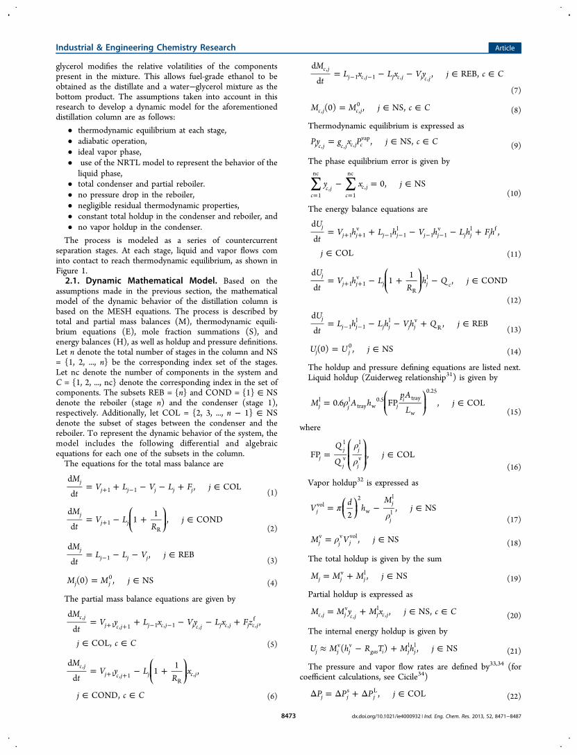
Figure 3. Perturbations in feed composition.

Table 5. Values of Reboiler Duty and Molar Reflux Ratio forthe Uncontrolled Simulation

parameter value

RR 0.04QR 5.9784 GJ/h




5. CASE STUDY

To successfully accomplish the simulation and optimization ofthe extractive distillation column, certain physical propertiesand column elements of the system have to be determined,namely, vapor pressure, heat capacities, liquid-phase activity

coefficients, densities, heats of vaporization, and columninternal characteristics, as noted by eqs 1−30. The way thesephysical properties were calculated is summarized in Table 3.Column internal characteristics were obtained with a steady-state simulation of the column in Aspen Plus45 and with

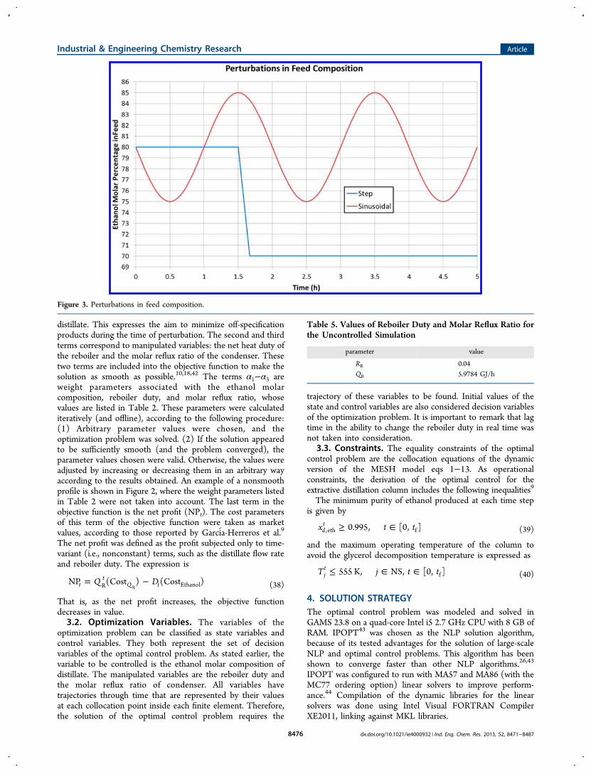
Figure 4. Uncontrolled response of the extractive column with a sinusoidal perturbation.

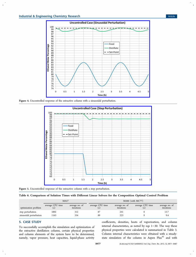
Figure 5. Uncontrolled response of the extractive column with a step perturbation.

Table 6. Comparison of Solution Times with Different Linear Solvers for the Composition Optimal Control Problem

MA57 MA86 (with MC77)

optimization problemaverage CPU time

(s)average no. ofiterations

average CPU time(s)

average no. ofiterations

average CPU time(s)

average no. ofiterations

step perturbation 1002 312 87 241 8 13.7sinusoidal perturbation 1163 334 89 223 9 9.4





expressions retrieved from Aspen Plus according to Zuiderweg’sexpression,31 as summarized in Table 4.The dynamic behavior of the extractive distillation system

was simulated to obtain its uncontrolled response to two typesof perturbations in the feed conditions.5.1. Operating Conditions. The extraction column is

made up of a total condenser (stage 1), 17 theoretical stages,and a partial reboiler (stage 19). The azeotropic mixture is fedinto stage 12 at a rate of 100 kmol/h and at saturated liquidconditions (i.e., Tf = 351 K). Pure glycerol is fed into stage 3 ata rate of 35 kmol/h and a temperature of 305 K. The condenseroperates at atmospheric pressure (101 kPa), and pressure dropis calculated with the preceding equations. These operatingconditions are the same as reported by Garcia-Herreros et al.,9

except for the azeotropic feed temperature, glycerol feed rateand pressure drop across the column. The saturated liquidtemperature in the azeotropic feed was used instead ofsubcooled liquid temperature (reported by Garcia-Herreroset al.9), and a lower value of the glycerol feed rate was used(35 instead of 52 kmol/h reported by Garcia-Herreros et al.9).The latter change was made because, in preliminary optimiza-tions, it was found that, by defining the glycerol feed rate as atime-independent variable, its optimal value for any type ofoptimization problem was 35 kmol/h. As a consequence, thatvalue was assumed constant in the present research. Theazeotropic mixture composition was subjected to two different

disturbances to obtain the optimal control profiles for the twoscenarios.

5.2. Perturbations. For the derivation of the optimalcontrol, two different types of perturbations were taken intoaccount: the sinusoidal one described by eq 41 and a stepperturbation. The two perturbations were defined as shown inFigure 3. The sinusoidal perturbation in ethanol molarcomposition was defined as

π= − ∈z t i80 5sin( ), timei i,ethf

(41)

where ti stands for time (h). The dynamic behavior of thesystem was evaluated in a 5-h span of operation.

5.3. Uncontrolled Response. The uncontrolled responseof the dynamic system was obtained by assuming that themanipulated variables of the column, the condenser molar refluxratio (RR) and reboiler heat duty (QR), were considered constant intime (Table 5) according to the results of Garcia-Herreros et al.9

The response of the dynamic system is shown in Figures 4 and 5.As can be observed, the ethanol composition in the distillate

was out of specification because, in some time intervals, it wasbelow 99.5% on a molar basis. It was thus necessary to derivethe optimal control strategy of the extractive distillation columnto guarantee the production of fuel-grade ethanol and tomaximize the profit of the process.

6. RESULTSIt was found that the MA86 linear solver was faster than theMA57 solver, because it was more recently developed and canrun in parallel, exploiting multiprocessor architecture.44

Dramatic changes in solution times were observed withMA86, decreasing from 1150 CPU s (MA57) to 84 CPU s(MA86) in some cases. Table 6 reports the different CPU timesobserved with different linear solvers and the solver times wheninitialized with a warm start (i.e., with the results obtainedfrom the previous optimization). The optimization probleminvolved 38457 variables and 38425 constraints (31 inequalities,

Table 7. Steady-State Simulations with Different RefluxRatio and Reboiler Duty Values to Obtain Different NLPInitializations

initialization reflux ratio reboiler duty (GJ/h)

1 0.2 5.82 0.04 5.97843 0.1 5.5

Figure 6. Optimal profile of ethanol composition in the distillate.




38394 equalities), leading to 62 degrees of freedom(manipulated variables). It is important to note that, withMA86 solution times, an NMPC control strategy can be reliableand successfully implemented, because these times are very lowcompared to the prediction horizon of an NMPC,27 even moreso when the optimal control problem is started warm, in whichcase the solution times are very low.6.1. Initialization. For the initialization of the optimization

problem, the steady-state values of the variables at each timestep were chosen. It is important to remark that theconvergence of the algorithm is highly dependent on theinitialization values. Therefore, three different initializationswere used. Steady-state values were obtained by carrying out

steady-state simulations with different values of reflux ratio andreboiler duty, obtaining temperature, molar compositions(liquid and vapor), and liquid and vapor molar flow rateprofiles. Running the NLP problem with three differentinitializations (see Table 7) also resulted in the identificationof different local optima.10

6.2. Optimization Results. Comparative profiles of thedecision variables for the different perturbations are shown inFigures 6−18. It should be noted that figures of the optimaldistillate rate profile are included. This is important because thecontrolled overall process also has to maintain productivity, tosatisfy product demand. It can also be seen that the ethanolcomposition in the distillate was controlled by changing the

Figure 7. Optimal reboiler duty profile.

Figure 8. Optimal molar reflux ratio profile.





manipulated variables. A comparison between the optimal controlstrategy studied in this research and a simple equivalentproportional−integral (PI) scheme is shown in Figures 10−13,using PI tuning parameters as optimization variables. At this point,it is important to make some remarks about the compositioncontrol. As can be seen, the control strategy employed requiresreal-time knowledge of the distillate composition. In a commercialsetting, analyzers that can potentially provide composition analysisof a multicomponent stream include46 gas chromatographs,infrared spectrometers, UV spectrometers, mass spectrometers,and nuclear magnetic resonance (NMR) analyzers. Of these, gaschromatography is most commonly applied to distillationcolumns.46 That is, online composition analyzers have a solid

advantage: They report the value of the composition in astraightforward manner.46 However, they also have importantdrawbacks:46 Installation and maintenance costs are very high,highly specialized technicians are required to perform maintenanceand operation, and they have considerable lag times. Another wayto infer the composition of a column product is by usingtemperature. If a constant temperature is maintained for aspecified stage, the composition of the product stream will remainessentially constant.46,47 The advantage of this approach is thattemperature measurements have very little or no lag time, aremore reliable, and entail very low installation and maintenancecosts. For these reasons, an optimization problem in which thecontrolled variable was a specified stage temperature was also

Figure 9. Optimal distillate flow rate profile.

Figure 10. Ethanol composition profile: PI controller versus optimal composition control.





taken into consideration, for only the sinusoidal perturbation(Figures 14−18). The most sensitive tray temperature forcomposition control was selected using the sensitivity criterionof Luyben.48 The analysis determined the stage 4 temperature tobe the most sensitive to distillate composition.In all cases, the objective function optimal value was found to

be negative, indicating the reliability of the overall controlledprocess. The PI parameters found by the solution of the PIcontrol optimization problem are reported in Table 8.

7. ANALYSIS AND DISCUSSION

Analysis and discussion of each set of figures displayed in thepreceding section is presented next. Table 9 lists the objectivefunction values for all of the optimal control problems considered inthis work.

7.1. Composition Control. The optimal profiles in Figures6−9 show the optimal behavior of the decision variables for thecomposition control case. As can be observed, the ethanolcomposition in the distillate can be maintained constant despitethe different perturbations in feed conditions. It is important toremark that manipulated variables responded in a mannerconsistent with the perturbation in the feed and managed tokeep the system in the required operation point and tominimize off-specification product. The manipulated variablesexhibited different frequenc ies with respect to the frequency ofthe feed perturbation49 in the sinusoidal case. This is aconsequence of system inertia (i.e., molar holdup in trays).A delay in response in both cases can be seen clearly, tak-ing into account that the overshoot is not significant inmagnitude.

Figure 11. Reboiler duty profile: PI controller.

Figure 12. Reflux ratio profile: PI controller.





On the other hand, it is important to remark that, althoughthe task of the control system is to maintain the ethanolcomposition in the distillate at a given operation point, it is alsoimportant not to sacrifice distillate flow (i.e., ethanolthroughput), as stated earlier. Figure 9 shows that this task ispossible most notably in the sinusoidal perturbation case: Thedistillate flow rate oscillates between ∼74 and ∼84 kmol/h,weighting the deviation with the steady-state optimization. Itcan also be seen that the set-point values of the reboiler dutyand reflux ratio differ from the set points in the sinusoidalperturbation case. This result is consistent with the inclusion ofthe steady-state variables (set points) in the optimizationproblem, on the framework of the multiplicity of the steadystates of the extractive distillation process.11,12 The optimalpoint is reached by changing the set-point values of bothvariables. Moreover, from Table 9, the higher value of the

objective function in the sinusoidal perturbation case is notable.All objective function values (at the optimal point) were foundto be negative, indicating the economic reliability of the overallcontrolled process. The control terms (first three terms) of thecomposite objective function (at the optimal point) were verysmall compared with the profit term.The optimization was performed with the three different

initializations listed in Table 7 to increase the probability offinding the global optimum within variable bounds. The resultsobtained with the three different initializations were exactly thesame. This confirms that at least a very good local optimum waslikely found.On the other hand, to analyze whether an improvement in

the overall profit could be obtained with the compositeobjective function (eq 37), an optimization was carried out witha control-only objective function (first three terms of eq 37)

Figure 13. Distillate flow rate profile: PI controller versus optimal composition control.

Figure 14. Ethanol composition profile in distillate: temperature control versus composition control.





with the sinusoidal perturbation. Table 10 indicates that theoverall profit (computed according to the negative of eq 38)was greater for the composite objective function.7.2. PI versus Optimal Control. As can be seen from

Figures 10−13, the PI control strategy was also capable ofmaintaining the ethanol composition above 99.5% on a molarbasis. However, it is clear from Figure 10 that the response wasnot as smooth as for optimal control. As shown in the profilesof the manipulated variables, the results of the PI control

strategy differed notably from those of the optimal controlstrategy. This is because the manipulated variables in a PIcontrol strategy have to respond according to the PI controllermodel equations, whereas in the optimal control case (as in anNMPC controller), the manipulated variables can respondfreely within variable bounds. It is important to note that the PIcontroller maintains the ethanol composition above the desired

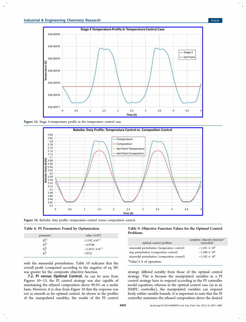
Figure 15. Stage 4 temperature profile in the temperature control case.

Figure 16. Reboiler duty profile: temperature control versus composition control.

Table 8. PI Parameters Found by Optimization

parameter value (×105)

KPQR 1.1192 ×10−5

KIQR −4.9788

KPRR −2.2813 ×10−5

KIRR 7.0731

Table 9. Objective Function Values for the Optimal ControlProblems

optimal control problemcomplete objective functiona

(unscaled)

sinusoidal perturbation (temperature control) −1.181 × 104

step perturbation (composition control) −1.100 × 104

sinusoidal perturbation (composition control) −1.182 × 104

aValue/5 h of operation.





set point but keeps the ethanol throughput lower than in theoptimal control case, for this very reason. Other authors havereported similar results for comparisons between model-basedcontrol strategies and traditional PI control schemes.30,50

7.3. Temperature versus Composition Control. FromFigures 14−18, it is clear that controlling the temperature on aspecified stage allows the ethanol composition in the distillateto be maintained above 99.5% on a molar basis with a smoothresponse. The temperature of stage 4 was maintained almostconstant, oscillating in only a small interval. It should be noted

that results of the temperature-control strategy were verysimilar to those of the composition-control strategy. This isbecause, although controlling the temperature of a stage is notthe same as directly controlling the distillate composition, it isat least equivalent and reliable. The ethanol throughput andreboiler duty profiles in both the temperature- andcomposition-control cases were very similar, indicating thatthe profits of the two processes were practically the same, asshown by the objective function values in Table 9.

8. CONCLUSIONS

The derivation of the optimal control strategy for the extractivedistillation of fuel-grade ethanol was successfully addressed inthis work. Using state-of-the-art algorithms, the solution of thislarge-scale problem can be obtained in a matter of minutes oreven seconds in the case of a warm start of the optimization

Figure 17. Reflux ratio profile: temperature control versus composition control.

Figure 18. Distillate flow rate profile: temperature control versus composition control.

Table 10. Comparison of the Profit Value in DifferentOptimization Problems (Composition Control)

optimization problem profit ($/5 h of operation)

control-only 7885.09composite (sinusoidal) 11851.49





problem. Our experience using different linear solvers withIPOPT shows that MA86 (with MC77) performs very well andbehaves well with the large-scale NLP derived from the optimalcontrol problem. With this type of results, it can be concludedthat it is possible to implement an NMPC control strategy forthis kind of process having several advantages over traditionalPI control systems, using rigorous, nonideal, and highlynonlinear models.It is also shown that, through optimization, it is possible to

find the optimal control strategy of such a change-prone systemas extractive distillation, even when the modeling is doneconsidering a great number of nonidealities such as vaporholdup and pressure drop. The solution of several differentproblems addressed in this research confirms this statement.On the other hand, it is also shown that, whether controllingthe distillate composition or the temperature of a specific stage,the control system behaves properly and responds in a mannerconsistent with the disturbances to minimize off-specificationproduct.It is also notable that the controllability of the extractive

distillation process was confirmed, showing that the designedprocess proposed by Garcia-Herreros et al.9 is not only stableand operable in steady-state operation but also subjected todynamic disturbances in theory.This type of optimization problem has multiple local minima

because of the nonconvexities in the model, although IPOPTwas able to find the local optima inside the feasible region inmost cases. This was also confirmed by solving most of theproblems with three different initializations. The resultsobtained showed an economically profitable process evenwhen the process itself was subjected to strong perturbations inits operating conditions, such as those proposed in thisresearch.As future work, we propose the simultaneous design and

optimal control of an extractive distillation column and, further,a complete extraction/recovery system. On the other hand, wewill address the complete NMPC control strategy of anextractive distillation column in upcoming research.

■ AUTHOR INFORMATIONCorresponding Author*E-mail: [email protected] authors declare no competing financial interest.

■ ACKNOWLEDGMENTSWe thank HSL for providing the linear solver subroutines freeof charge for academic purposes.

■ NOMENCLATUREA0 = hole tray area (m)Atray = total active bubbling area on the tray (m2)C = index set of componentsCostEthanol = ethanol price ($/kmol)CostQR

= reboiler duty cost ($/GJ)d = column diameter (m)di = design parameterFj = feed molar flow rate at stage j (kmol/h)f ja = aeration factorFP = flow parameterg = acceleration of gravity (m/s2)h = distance between finite elements

hj = total molar enthalpy (GJ) at stage jhjD = liquid height below the weir of stage j (m)hw = average weir height (m)I = total number of finite elementsK = total number of collocation pointsK0 = hole coefficientLj = liquid molar flow rate at stage j (kmol/h)Lw = average weir length (m)Mc,j = molar holdup of component c at stage j (kmol)Mj = total molar holdup at stage j (kmol)Mj

l = liquid molar holdup at stage j (kmol)Mj

v = vapor molar holdup at stage j (kmol)n = total number of stagesnc = total number of componentsNP = net profit ($)NS = index set of stagesp = design parameterPc

vap = vapor pressure (MPa) of component cpi = diameter of tray holes (m)Pj = absolute pressure of stage j (MPa)Qcond = condenser duty (GJ/h)Qj = volumetric flow rate at stage j (m3/h)QR = reboiler duty (GJ/h)Rgas = ideal-gas constant [MJ/(kmol K)]RR = condenser molar reflux ratiotf = final time (h)ui,k = control profile at finite element i, collocation point kUj = internal energy holdup at stage j (MJ)Vj = vapor molar flow rate at stage j (kmol/h)Vjvol = vapor volume at stage j (m3)

xc,j = liquid molar composition of component c at stage jyc,j = vapor molar composition of component c at stage jZf = molar composition in the feedzi,k = state profile at finite element i, collocation point k

Greek Symbols

αi = weight parameterγc,j = liquid-phase activity coefficient of component c at stagejΔPj = pressure drop of stage j (mmHg)ΔPjL = liquid pressure drop of stage j (mmHg)ΔPjS = dry tray pressure drop of stage j (mmHg)ε = tray porosityρj = molar density (kmol/m3) at stage jτ = Radau collocation pointΩ = collocation matrix

Subscripts

c = chemical speciesd = distillateeth = ethanoli = finite elementj = tray numberk = collocation pointti = time

Superscripts

f = feedl = liquid phasesp = set pointt = timev = vapor phase



mailto:[email protected]

■ REFERENCES(1) Agrawal, R.; Mallapragada, D. S.; Ribeiro, F. H.; Delgass, W. N.Novel Pathways for Biomass-to-Liquid Fuel Production. Presented atthe 2011 AIChE Annual Meeting, Minneapolis, MN, Oct 16−21, 2011.(2) Farrell, A. E.; Plevin, R. J.; Turner, B. T.; Jones, A. D.; O’Hare,M.; Kammen, D. M. Ethanol Can Contribute to Energy andEnvironmental Goals. Science 2006, 311, 506−508.(3) De Oliveira, M.; Vaughan, B. E.; Rykiel, E. J. Ethanol as Fuel:Energy, Carbon Dioxide Balances, and Ecological Footprint. BioScience2005, 55, 593.(4) Ministerio de Ambiente y Desarrollo Territorial Resolucion No.0447 de abril 14 de 2003, Bogota, Colombia; http://www.alcaldiabogota.gov.co/sisjur/normas/Norma1.jsp?i=15720 (accessedNovember 2011).(5) Gil, I. D.; Gomez, J. M.; Rodríguez, G. Control of an ExtractiveDistillation Process to Dehydrate Ethanol Using Glycerol as Entrainer.Comput. Chem. Eng. 2012, 39, 129−142.(6) Bastidas, P. A.; Gil, I. D.; Rodríguez, G. Comparison of the MainEthanol Dehydration Technologies Through Process SimulationPresented at the 20th European Symposium on Computer Aided ProcessEngineering, Naples, Italy, Jun 6−9, 2010(7) Real Prospects for Energy Efficiency in the United States; TheNational Academies Press: Washington, DC, 2010.(8) Seider, W. D.; Seader, J. D.; Lewin, D. R. Process Design Principles:Synthesis, Analysis, and Evaluation; Wiley: New York, 1999.(9) García-Herreros, P.; Gomez, J. M.; Gil, I. D.; Rodríguez, G.Optimization of the Design and Operation of an Extractive DistillationSystem for the Production of Fuel Grade Ethanol Using Glycerol asEntrainer. Ind. Eng. Chem. Res. 2011, 50, 3977−3985.(10) Lo pez-Negrete de la Fuente, R.; Flores-Tlacuahuac, A.Integrated Design and Control Using a Simultaneous Mixed-IntegerDynamic Optimization Approach. Ind. Eng. Chem. Res. 2009, 48,1933−1943.(11) Rovaglio, M.; Doherty, M. F. Dynamics of HeterogeneousAzeotropic Distillation Columns. AIChE J. 1990, 36, 39−52.(12) Esbjerg, K.; Andersen, T. R.; Muller, D.; Marquardt, W.;Jørgensen, S. B. Multiple Steady States in Heterogeneous AzeotropicDistillation Sequences. Ind. Eng. Chem. Res. 1998, 37, 4434−4452.(13) Prokopakis, G. J.; Seider, W. D. Feasible Specifications inAzeotropic Distillation. AIChE J. 1983, 29, 49−60.(14) Gilles, E. D.; Retzbach, D.; Silberberger, F. Modeling,Simulation and Control of an Extractive Distillation Column. InComputer Applications to Chemical Engineering; ACS SymposiumSeries; American Chemical Society: Washington, DC, 1980; Vol.124, pp 481−492.(15) Gani, R.; Romagnoli, J. A.; Stephanopoulos, G. Control Studiesin an Extractive Distillation Process: Simulation and MeasurementStructure. Chem. Eng. Commun. 1986, 40, 281−302.(16) Choe, Y. S.; Luyben, W. L. Rigorous Dynamic Models ofDistillation Columns. Ind. Eng. Chem. Res. 1987, 26, 2158−2161.(17) Arifin, S.; Chien, I.-L. Design and Control of an IsopropylAlcohol Dehydration Process via Extractive Distillation UsingDimethyl Sulfoxide as an Entrainer. Ind. Eng. Chem. Res. 2008, 47,790−803.(18) Ghaee, A.; Gharebagh, R. S.; Mostoufi, N. DynamicOptimization of the Benzene Extractive Distillation Unit. Braz. J.Chem. Eng. 2008, 25, 765−776.(19) Luyben, W. L. Effect of Solvent on Controllability in ExtractiveDistillation. Ind. Eng. Chem. Res. 2008, 47, 4425−4439.(20) Maciel, M. R. W.; Brito, R. P. Evaluation of the DynamicBehavior of an Extractive Distillation Column for Dehydration ofAqueous Ethanol Mixtures. Comput. Chem. Eng. 1995, 19 (Suppl. 1),405−408.(21) Barreto, A. A.; Rodriguez-Donis, I.; Gerbaud, V.; Joulia, X.Optimization of Heterogeneous Batch Extractive Distillation. Ind. Eng.Chem. Res. 2011, 50, 5204−5217.(22) Magnussen, T.; Michelsen, M.; Fredenslund, A. AzeotropicDistillation Using UNIFAC. Inst. Chem. Eng. Symp. Ser. 1976, 56, 1−19.

(23) Abu-Eishah, S. I.; Luyben, W. L. Design and Control of a Two-Column Azeotropic Distillation System. Ind. Eng. Chem. Process Des.Dev. 1985, 24, 132−140.(24) Cuthrell, J. E.; Biegler, L. T. On the Optimization of Differential-Algebraic Process Systems; Carnegie Mellon University: Pittsburgh, PA,1986.(25) Cuthrell, J. E.; Biegler, L. T. Simultaneous Optimization andSolution Methods for Batch Reactor Control Profiles; Carnegie MellonUniversity: Pittsburgh, PA, 1987.(26) Biegler, L. T. Nonlinear Programming: Concepts, Algorithms, andApplications to Chemical Processes; MPS-SIAM Series on Optimization;Society for Industrial and Applied Mathematics: Philadelphia, PA,2010.(27) Zavala, V. M.; Laird, C. D.; Biegler, L. T. Fast Implementationsand Rigorous Models: Can Both Be Accommodated in NMPC? Int. J.Robust Nonlinear Control 2008, 18, 800−815.(28) Biegler, L. T. Efficient Solution of Dynamic Optimization andNMPC Problems. Prog. Syst. Control Theory 2000, 26.(29) Zavala, V. M.; Biegler, L. T. Nonlinear Programming Strategiesfor State Estimation and Model Predictive Control. In Nonlinear ModelPredictive Control; Magni, L., Raimondo, D. M., Allgower, F., Eds.;Springer: Berlin, 2009; Vol. 384, pp 419−432.(30) Khaledi, R.; Young, B. R. Modeling and Model PredictiveControl of Composition and Conversion in an ETBE ReactiveDistillation Column. Ind. Eng. Chem. Res. 2005, 44, 3134−3145.(31) Zuiderweg, F. J. Sieve Trays: A View on the State of the Art.Chem. Eng. Sci. 1982, 37, 1441−1464.(32) Raghunathan, A. U.; Soledad Diaz, M.; Biegler, L. T. An MPECFormulation for Dynamic Optimization of Distillation Operations.Comput. Chem. Eng. 2004, 2037−2052.(33) Perry, R. H.; Green, D. W. Perry’s Chemical Engineers’ Handbook;McGraw-Hill: New York, 2007.(34) Cicile, J.-C. Distillation. Absorption - Colonnes a plateaux:Dimensionnement. Tech. Ing., Genie Procedes 1994, J2623.(35) Kooijman, H. A.; Taylor, R. The ChemSep Book; Books onDemand: Norderstedt, Germany, 2000.(36) Taylor, R.; Krishna, R. Multicomponent Mass Transfer; Wiley:New York, 1993.(37) Lang, Y.-D.; Biegler, L. T. Distributed Stream Method for TrayOptimization. AIChE J. 2002, 48, 582−595.(38) Cuthrell, J. E. On the Optimization of Differential-AlgebraicSystems of Equations in Chemical Engineering. Ph.D. Dissertation,Carnegie Mellon University, Pittsburgh, PA, 1986.(39) Diwekar, U. Batch Distillation: Simulation, Optimal Design, andControl, 2nd ed.; CRC Press: Boca Raton, FL, 2012.(40) Gerdts, M. Direct Shooting Method for the Numerical Solutionof Higher-Index DAE Optimal Control Problems. J. Optim. TheoryAppl. 2003, 117, 267−294.(41) Biegler, L. An overview of simultaneous strategies for dynamicoptimization. Chem. Eng. Process.: Process Intensif. 2007, 46, 1043−1053.(42) Miranda, M.; Reneaume, J. M.; Meyer, X.; Meyer, M.; Szigeti, F.Integrating Process Design and Control: An Application of OptimalControl to Chemical Processes. Chem. Eng. Process.: Process Intensif.2008, 47, 2004−2018.(43) Wachter, A.; Biegler, L. T. On the Implementation of anInterior-Point Filter Line-Search Algorithm for Large-Scale NonlinearProgramming. Math. Program. 2005, 106, 25−57.(44) A Collection of Fortran Codes for Large Scale ScientificComputation; HSL Mathematical Software Library: Harwell, Oxford,U.K., 2013; http://www.hsl.rl.ac.uk (accessed January 2012).(45) aspenONE, version: 7.2; Aspen Technology: Cambridge, MA,2008.(46) Smith, C. Distillation Control: An Engineering Perspective; JohnWiley & Sons: New York, 2012.(47) Kister, H. Z. Distillation Operation; McGraw-Hill: New York,1990.(48) Luyben, W. L. Distillation Design and Control Using AspenSimulation; Wiley-Interscience: New York, 2006.



http://www.alcaldiabogota.gov.co/sisjur/normas/Norma1.jsp?i=15720

http://www.alcaldiabogota.gov.co/sisjur/normas/Norma1.jsp?i=15720

http://www.hsl.rl.ac.uk

(49) Ross, R.; Perkins, J. D.; Pistikopoulos, E. N.; Koot, G. L. M.;Van Schijndel, J. M. G. Optimal Design and Control of a High-PurityIndustrial Distillation System. Comput. Chem. Eng. 2001, 25, 141−150.(50) Allgower, F.; Findeisen, R.; Zoltan, N. Nonlinear ModelPredictive Control: From Theory to Application. J. Chin. Inst. Chem.Eng. 2004, 299−316.



Optimal Control of the Extractive Distillation for the Production of Fuel-Grade Ethanol

Documents