Optimal Compensation and Implementation for Adaptive Optics Systems

OPTIMAL COMPENSATION AND IMPLEMENTATION FORADAPTIVE OPTICS SYSTEMS

DOUGLAS P. LOOZE1,∗, MARKUS KASPER2, STEFAN HIPPLER3, ORHAN BEKER1

and ROBERT WEISS3

1Department of Electrical and Computer Engineering, University of Massachusetts,Amherst, MA 01003, U.S.A.

2European Southern Observatory, Garching, Germany3Max Planck Institut fur Astronomie, Heidelberg, Germany(∗author for correspondence, e-mail: [email protected])

(Received 29 September 2003; accepted 23 February 2004)

Abstract. This paper develops a compensation algorithm based on Linear–Quadratic–Gaussian(LQG) control system design whose parameters are determined (in part) by a model of the atmo-sphere. The model for the atmosphere is based on the open-loop statistics of the atmosphere asobserved by the wavefront sensor, and is identified from these using an auto-regressive, moving aver-age (ARMA) model. The (LQG) control design is compared with an existing compensation algorithmfor a simulation developed at ESO that represents the operation of MACAO adaptive optics systemon the 8.2 m telescopes at Paranal, Chile.

Keywords: adaptive optics, astronomy, feedback systems, identification, optimal control

1. Introduction

Adaptive optics (AO) systems enhance the capability of ground-based astronomi-cal observation by reducing the effects of atmospheric refractive index variations.AO systems have been successfully implemented in several observatories, and anumber of scientific results based on observations from systems using AO havebeen reported (cf. Roddier et al., 1996; Duchene et al., 2002; Hackenberg et al.,2000). Still, current AO systems can be improved, both in terms of their basicperformance and in the reliability and simplicity of operation over the variety ofoperational environments experienced in observatories.

Among the many technologies that are integrated by AO systems is the compen-sation algorithm. The purpose of the compensation algorithm is to provide dynamicfeedback of the sensed wavefront to drive a deformable mirror (DM), with the ob-jective of minimizing aberrations that are added to the optical path prior to theDM. A number of different compensation algorithms have been developed and im-plemented. Adaptive optics compensators can be classified as zonal algorithms ormodal algorithms. Zonal compensation determines the actuation voltages appliedto the DM using estimates of the local wavefront phase error. Modal algorithms

Experimental Astronomy 15: 67–88, 2003.C© 2004 Kluwer Academic Publishers. Printed in the Netherlands.

68 D.P. LOOZE ET AL.

decompose the wavefront error into geometrically orthogonal modes, and com-pensate each mode individually. This paper considers modal control algorithms,although a similar approach can be used to implement a zonal compensation.

The most common control algorithm uses an integrator to generate the feedbacksignal (Gendron and Lena, 1994). The gains of the integral feedback can be adjustedindependently for each mode (Gendron and Lena, 1994; Dessenne et al., 1998), andthe controller can add dynamic compensation to the integration (Wirth et al., 1998;Dessenne et al., 1997).

The purpose of this paper is to develop a modal compensation algorithm basedon Linear–Quadratic–Gaussian (LQG) control system design. An LQG design willbe essentially the same as a modal design with dynamic compensation, but the pa-rameters of the compensator will be determined by the specification of the quadraticoptimization problem. The wavefront from a guidestar is measured by a wavefrontsensor (WFS), and decomposed into optical modes. The objective for any modaldesign is to have the modal coefficient of the wavefront phase reflected from the DMto be as near to zero as possible. The LQG design incorporates this objective by se-lecting the control parameters to minimize the square of the modal coefficient. TheLQG design is, therefore, based on the plant, disturbance and measurement models,as well as the objective functional. The design incorporates both the strength andweaknesses of these models.

An LQG modal compensation design will be a function of the model that rep-resents the effect of the earth’s atmosphere on the wavefront phase projected ontothe modal subspace. Kolmogorov statistics in thin turbulent layers are commonlyassumed (Tatarski, 1961) to develop atmospheric models. These models becomeinaccurate at high and low spatial frequencies (the inner and outer scale of turbu-lence), and depend on the coherence distance r0 and wind directions of each layer.The coherence distance, the inner and outer scales, the wind directions of each layerand the number of significant layers can change over time (usually several minutesto several hours).

Paschall and Anderson (1993) have designed a centralized AO controller usingan LQG formulation similar to the formulation in this paper. This design incor-porated the first 14 Zernike modes (ignoring the piston mode). Their spectra wereapproximated with first-order, independent Markov models. The mirror dynamicswere also modeled using first-order lags, and a one sample loop delay was incorpo-rated in the model. Measurement noise correlations were modeled from a Shack–Hartman sensor. The resulting LQG design determined the control for one Zernikecoefficient as a function of all the modeled Zernike coefficients and their delayedvalues. The controller for the chosen Zernike model was a fully populated, 42nd(three times the number of modes)-order transfer function. To compute this con-troller, two 42nd-order Riccati equations had to be solved. Using a similar model,the modal control of this paper would result in a separate third-order controllerfor each mode. Both the computation required to determine the controller, and thecomputations required at each sample would be significantly reduced for the modal

COMPENSATION AND IMPLEMENTATION FOR ADAPTIVE OPTICS SYSTEMS 69

controller. The computational differences become even greater as the number ofZernike modes considered increases. Since the number of modes of current AOsystems is large and since a changing atmosphere can require the computation of anew controller as often as a few minutes, solution of a large-order Riccati equationcan become impractical.

Several authors have optimized the integrator gain with respect to the atmo-spheric statistics. Gendron and Lena (1994, 1995) used an open-loop sample of anobserved star to determine the measurement noise (although a procedure, attributedto Rousset, was later found to be more efficient and as effective (Gendron and Lena,1995)) and turbulence power. This open-loop sample was then used to optimize theintegrator gains for each mode.

Dessenne et al. (1998) also obtained the AO compensation parameters by opti-mizing a performance index based on an approximation to the wavefront error. Theatmospheric statistics are again obtained from observed data and are used directlyto determine the compensator parameters. This paper uses a similar concept for se-lecting the compensator parameters, but separates the overall optimization probleminto two parts: identification of the atmosphere dynamics and compensator design.

This paper will use an infinite-time-horizon criterion (Kwakernaak and Sivan,1972; Anderson and Moore, 1990) to obtain a linear, time-invariant compensatorfor each mode. The compensation design problem is formulated as an optimaldisturbance rejection problem in discrete-time, with the objective of minimizing theRMS wavefront phase error orthogonal to the piston mode. The modal disturbancesare determined from identifying the effects of the atmosphere. The disturbancesare modeled as white noise passed through a finite dimensional filter. Open-loopobservations of a guidestar are obtained, and a finite-order model is fitted to themeasurements. Each modal noise is then determined from the fitted transfer functionusing a procedure analogous to that of Rousset (Gendron and Lena, 1995). Finally,the measurement noise spectrum is subtracted from the identified spectrum, andthe result appropriately factored to obtain the parameters of the disturbance filter.

Each modal disturbance rejection problem is then an LQG optimal control prob-lem with no weighting on the control. The LQG modal disturbance problems can beeasily solved, and yield low-order compensators for most DMs and most identifiedatmospheric models.

The resulting LQG control design is compared with an existing compensationalgorithm. The LQG design that is used is based on a simulation developed at ESOto represent the MACAO system implemented on the 8.2 m telescopes at Paranal,Chile (Craven-Bartle et al., 2000).

2. The modal control adaptive optics problem

Adaptive optics systems attempt to eliminate the phase variations by varyingthe optical path length between the aperture and science instrument depending


on the location of the light in the aperture. The optical path length is modifiedby measuring the current phase variation via one or more WFS and (possibly)adjusting the orientation of a tip–tilt mirror (TTM) and the shape of the DMdynamically.

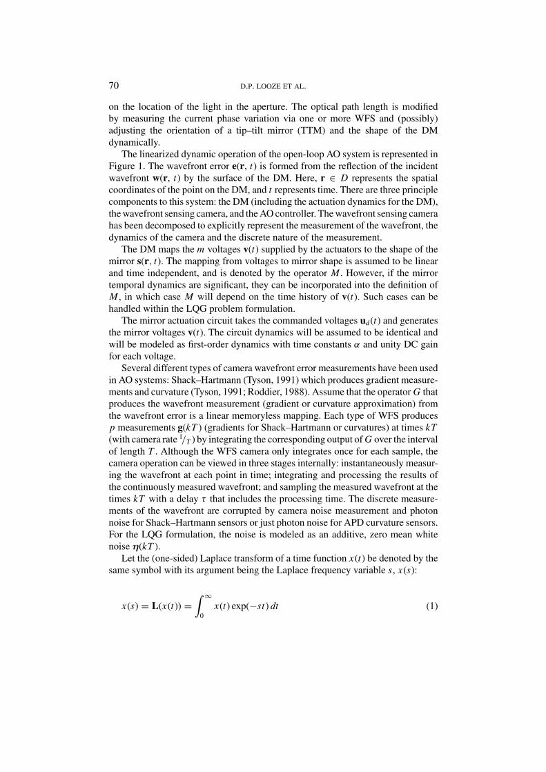
The linearized dynamic operation of the open-loop AO system is represented inFigure 1. The wavefront error e(r, t) is formed from the reflection of the incidentwavefront w(r, t) by the surface of the DM. Here, r ∈ D represents the spatialcoordinates of the point on the DM, and t represents time. There are three principlecomponents to this system: the DM (including the actuation dynamics for the DM),the wavefront sensing camera, and the AO controller. The wavefront sensing camerahas been decomposed to explicitly represent the measurement of the wavefront, thedynamics of the camera and the discrete nature of the measurement.

The DM maps the m voltages v(t) supplied by the actuators to the shape of themirror s(r, t). The mapping from voltages to mirror shape is assumed to be linearand time independent, and is denoted by the operator M . However, if the mirrortemporal dynamics are significant, they can be incorporated into the definition ofM , in which case M will depend on the time history of v(t). Such cases can behandled within the LQG problem formulation.

The mirror actuation circuit takes the commanded voltages ud(t) and generatesthe mirror voltages v(t). The circuit dynamics will be assumed to be identical andwill be modeled as first-order dynamics with time constants α and unity DC gainfor each voltage.

Several different types of camera wavefront error measurements have been usedin AO systems: Shack–Hartmann (Tyson, 1991) which produces gradient measure-ments and curvature (Tyson, 1991; Roddier, 1988). Assume that the operator G thatproduces the wavefront measurement (gradient or curvature approximation) fromthe wavefront error is a linear memoryless mapping. Each type of WFS producesp measurements g(kT ) (gradients for Shack–Hartmann or curvatures) at times kT(with camera rate 1/T ) by integrating the corresponding output of G over the intervalof length T . Although the WFS camera only integrates once for each sample, thecamera operation can be viewed in three stages internally: instantaneously measur-ing the wavefront at each point in time; integrating and processing the results ofthe continuously measured wavefront; and sampling the measured wavefront at thetimes kT with a delay τ that includes the processing time. The discrete measure-ments of the wavefront are corrupted by camera noise measurement and photonnoise for Shack–Hartmann sensors or just photon noise for APD curvature sensors.For the LQG formulation, the noise is modeled as an additive, zero mean whitenoise η(kT ).

Let the (one-sided) Laplace transform of a time function x(t) be denoted by thesame symbol with its argument being the Laplace frequency variable s, x(s):

x(s) = L(x(t)) =∫ ∞

0x(t) exp(−st) dt (1)


Figure 1. Feedback loop for a general adaptive optics system.

Since the WFS camera forms the measurement by integrating the measuredfeature over one sample interval and includes a delay, the camera dynamics are:

Γ(s) = exp(−sτ )(1 − exp(−sT ))

sI, (2)

where I is the identity matrix. The measurement is assumed to be the sampled valueof the continuous integration within the WFS.

The zero-order hold (ZOH) in Figure 1 applies continuous commanded voltagesud(t) to the DM. The applied voltage between samples is constant and equal to thediscrete coefficients of the compensator commands at the preceding sample time.

The modal controller, the signal produced by the controller, and the cameraoutput in Figure 1 are all discrete time signals or systems, and are represented byZ -transforms. As in continuous time, the same function symbol will be used todenote the signal in either the discrete time or frequency domain. Let T representthe discrete-time sample period. Given a discrete-time function xk = x(kT ), itsone-sided Z -transform (analogous to the Laplace transform for continuous-timesignals) is defined as:

x(z) = Z{xk} =∞∑

k=0

xkz−k (3)

The control system in Figure 1 is represented by its discrete-time transfer func-tion Gc(z), (the Z -transform of the pulse response of the controller). Due to thefinite number of actuators and measurements, the controller has a finite numberof degrees of freedom. A modal controller restricts the controlled subspace to thedimension of the number of degrees of freedom by decomposing the wavefront.

The phase wavefront is statistically described in terms of the atmosphere phasestructure function. For a given structure function and a given aperture, the eigen-functions of the corresponding power spectrum (the Karhunen–Loeve modes cf.(Dai, 1995)) are geometrically orthonormal over the aperture, and uncorrelated.Zernike modes (Noll, 1976) are also geometrically orthogonal over the aperture,but are not uncorrelated. System modes (Donaldson et al., 2000) (eigenmodes of the


interaction matrix) have also been used for AO control design and implementation,but are neither uncorrelated nor geometrically orthogonal over the aperture. Theyare, however, geometrically orthogonal at the mirror controls.

The selection of the modal basis can be optimized for a specified AO system(Ellerbroek, 1994). For example, if an accurate model of the atmosphere structurefunction is available and sensor correlations are ignored, the best basis in termsof optimizing the energy in the modes is the Karhunen–Loeve basis. We will as-sume that any optimization of the basis has been done with a modal compensationarchitecture embedded in the selection process. We will also assume that the ba-sis selection (by whatever means) will not be affected by the compensator designchoice. Although any dependency between modes could, in principle, be exploitedby controller couplings, such couplings are not used by the modal control architec-ture.

Any wavefront can be represented in terms of a set of geometrically orthonormalmodes {ei (r)} as:

e(r, t) =∞∑

i=0

mi (t)ei (r), (4)

where the i = 0 mode is the piston mode. The power in each mode is non-increasingas i increases for i > 1 (Dai, 1995). For Zernike modes, the tip and tilt modes aremodes 1 and 2. In the Karhunen–Loeve basis, modes 1 and 2 contain significantglobal tilt and are near (as measured by the two-norm on the aperture) the tip andtilt modes of the Zernike basis.

A modal actuation matrix M∈Rm×nc is selected to apply the first nc modes to themirror. For Karhunen–Loeve and Zernike modes, the i th column of M is a sampledapproximation of the i th modal shape ei (r), and thus is only approximately geo-metrically orthogonal (and uncorrelated for Karhunen–Loeve modes). For systemmodes, the actuation matrix is the identity.

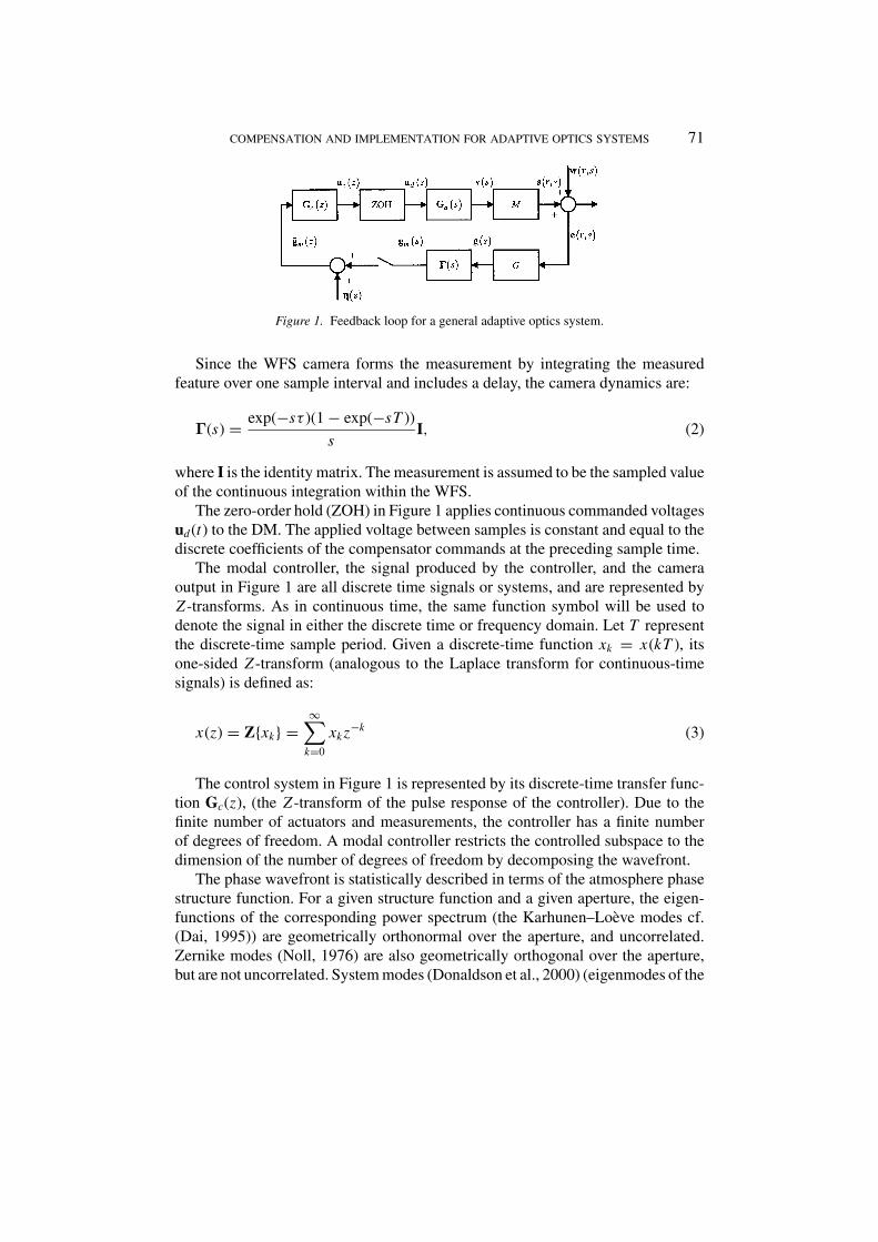
There are numerous methodologies to determine the reconstruction matrix.Wallner (1983) developed an optimal reconstructor for zonal estimation. Law andLane (1996) developed a maximum a posteriori (MAP) modal reconstructor andshowed that it was equivalent to Wallner’s zonal reconstructor. Kasper (2000) calcu-lated the closed-loop MAP using an expression for the closed-loop modal variancespresented in Veran et al. (1997). Dynamic reconstructors that use previous valuesof the controller have been developed by Wild (1996) to mitigate the effects ofdelay. It will be assumed that the reconstructor has been chosen and is representedby a (memoryless) matrix H∈Rnc×pthat estimates the i th modal coefficient fromthe WFS measurement. The architecture of the modal control system is shown inFigure 2.

The nominal stability and performance analyses of all modal compensationalgorithms rely on the modal subproblems being decoupled. DMs that have enoughactuators to reproduce the modes to be controlled will result in a complete or near


Figure 2. Feedback loop for an adaptive optics system using modal control.

decoupling (depending on the modal basis used) of the modal subproblems for PIand WLS reconstructors. The MAP reconstructor can result in significant couplingfor dim guidestars. This potential coupling would have to be considered if the MAPreconstructor were used.

3. Modal dynamic compensation problem

3.1. MODAL PROBLEM

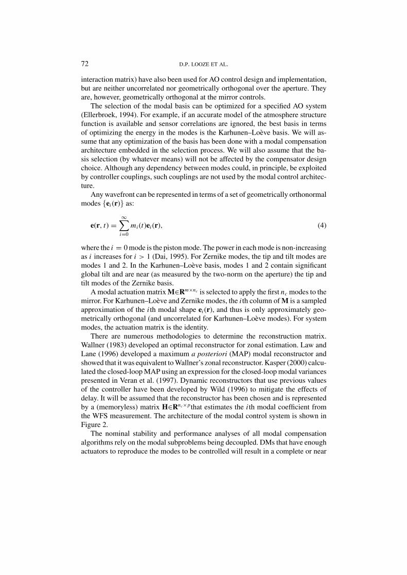
The modal control problem formulated in Section 2 can be assumed to decomposeinto nc modal control problems, where nc is the number of modes to be controlled.Each of the modal control problems is a scalar, discrete-time, modal control problemwith the structure shown in Figure 3. In Figure 3, all signals are the i th coefficient ofthe corresponding vector signal in modal coordinates. The input to the diagonal plantmodel (DM, actuators and WFS) is the modal command ui (z), and the output yi (z)is the mirror surface in modal coordinates. The disturbance di (z) affecting this loopis caused by the effects of atmospheric refraction. The measurement error projectedonto the modal subspace is denoted by ηi (z). The estimate of the i th mode mi (z)is the output of camera and reconstructor. The objective of the individual modalcontrol problems is to make the error signal mi (z) small.

Figure 3. Modal control subproblem.


The plant model Pi (z) is the same for each mode i , and is given by the diagonalelements of Pm(z) (see Figure 2). The disturbance to the loop in Figure 3 representsthe atmospheric aberrations affecting the modal coefficient of the phase wavefrontas determined by the WFS and reconstructor. This disturbance is given in discrete-time by the operation of the camera and reconstructor on the incoming wavefront:

di (z) = HZ{L−1{Γ(s)Gw(r, s)}}i , (5)

where the subscript on the right of (5) indicates the i th element of the vector andZ is the z-transform with sample time T (see (3)). The overall measurement noiseincludes both camera read-out noise and wavefront photon noise. Although thephoton noise is signal-dependent and Poisson, it will be approximated by a zeromean, white Gaussian process with power spectral density R. The modal noise ismodeled as independent:

ηi (z) = (Hη(z))i , (6)

with its power spectrum given by the i th diagonal element Ri .

3.2. STATE VARIABLE MODELS

3.2.1. Plant modelWhen the actuator time constant and mirror dynamics can be neglected, the delayτ introduces a set of zeros at the origin and one zero on the negative real axis.Specifically, the plant is given by

P(z) = S

{(1 − exp(−sT )) exp(−sτ )

s

}= (1 − z−1)2

×Z{

L−1

{exp(−sτ )

s2

}}, (7)

where the operator S{·} denotes the step-invariant model (Franklin et al., 1988).Let the computational delay be related to the camera frame rate by two pa-

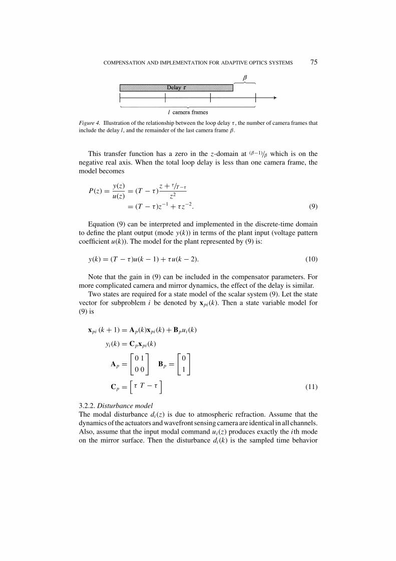
rameters (see Figure 4): l and β. The parameter l is the smallest number ofcamera frames greater than or equal to the delay: l ≥ τ/T . The parameter β isthe remainder of the last camera frame normalized by the camera frame. Thus,τ = (l − β)T, 0 < β ≤ 1. Note that the number of camera frames can often betaken to be l = 1. However, if the loop delay is greater than one camera frame,l > 1. For arbitrary l, Equation (7) becomes

P(z) = Tβz + 1 − β

zl+1. (8)


Figure 4. Illustration of the relationship between the loop delay τ , the number of camera frames thatinclude the delay l, and the remainder of the last camera frame β.

This transfer function has a zero in the z-domain at (β−1)/β which is on thenegative real axis. When the total loop delay is less than one camera frame, themodel becomes

P(z) = y(z)

u(z)= (T − τ )

z + τ/T −τ

z2

= (T − τ )z−1 + τ z−2. (9)

Equation (9) can be interpreted and implemented in the discrete-time domainto define the plant output (mode y(k)) in terms of the plant input (voltage patterncoefficient u(k)). The model for the plant represented by (9) is:

y(k) = (T − τ )u(k − 1) + τu(k − 2). (10)

Note that the gain in (9) can be included in the compensator parameters. Formore complicated camera and mirror dynamics, the effect of the delay is similar.

Two states are required for a state model of the scalar system (9). Let the statevector for subproblem i be denoted by xpi (k). Then a state variable model for(9) is

xpi (k + 1) = Ap(k)xpi (k) + Bpui (k)

yi (k) = Cpxpi (k)

Ap =[

0 1

0 0

]Bp =

[0

1

]

Cp =[τ T − τ

](11)

3.2.2. Disturbance modelThe modal disturbance di (z) is due to atmospheric refraction. Assume that thedynamics of the actuators and wavefront sensing camera are identical in all channels.Also, assume that the input modal command ui (z) produces exactly the i th modeon the mirror surface. Then the disturbance di (k) is the sampled time behavior


of the projection of the i th mode of the atmosphere. Finally, it will be assumedthat the loop disturbance can be approximately represented by a finite-dimensionaldiscrete-time model driven by unit variance white noise. A state variable modelwith state xdi (k) is given by

xdi (k + 1) = Adi xdi (k) + Bdiξi (k),

di (k) = Cdi xdi (k) + Ddiξi (k), (12)

where ξi (k) is a zero mean, unit variance white noise process.

3.2.3. Performance evaluationA common measure of AO performance is the Strehl ratio S (Tyson, 1991) of theimage produced by the system. Several approximations to the Strehl ratio are oftenused. For example, if the wavefront variance in the pupil σ 2

w is small, it can beshown (Tyson, 1991) that

S ≈ exp

(−

(2π

λ

)2

σ 2w

)≈ 1 −

(2π

λ

)2

σ 2w, (13)

where λ is the wavelength of the incoming beam. The important property illustratedby (13) is that the Strehl ratio is a strictly decreasing function of the wavefrontvariance. Hence the objective of minimizing the wavefront variance is equivalentto maximizing the Strehl ratio.

For an orthonormal modal basis set (with accurate approximations by the DMand WFS spatial sampling), the variance is the sum of the variances of the modalcoefficients. Assuming the system is ergodic, the variance is given by:

σ 2w = Lim

t→∞

∞∑i=1

E{m2

i (t)}, (14)

where mi (t) is the wavefront error from the i th modal control problem. The objec-tive for each of the modal control problems is to minimize the steady-state outputerror variance:

minui (t)

Limt→∞ E

{m2

i (t)}. (15)

Even if the modes are not orthogonal spatially on the telescope pupil (such assystem modes), minimizing the variance of each mode will still reduce the varianceof the overall wavefront.


4. Linear–Quadratic–Gaussian modal design

4.1. LINEAR–QUADRATIC–GAUSSIAN (LQG) PROBLEMS

This subsection presents the discrete-time LQG control problem, its solution andthe compensator that is obtained. Assume that the system is linear and time invariant(LTI) with state x(k), input u(k) and measurement y(k) given by the state variablemodel

x(k + 1) = Ax(k) + Bu(k) + Gξ (k)

y(k) = Cx(k) + Dξ (k) + η(k), (16)

with ξ (k) and η(k) zero-mean, Gaussian, white noise sequences with covariances Iand the symmetric, positive definite matrix , respectively. Note that the input tothe disturbance model is unit covariance white noise and is represented by ξ (k). Thestatistics of the disturbance entering the feedback loop in Figure 3 is governed bythe disturbance model (12), which is included in (16). The modal plant input u(k)is the modal command (output) of the compensator. The modal plant measurementy(k) is the reconstructed estimate of the modal coefficient, and is the input to themodal compensator.

The objective is to select u(k) to minimize the functional

J = limk→∞

E{xT (k) Qx(k)}, (17)

where Q is a symmetric, positive semi-definite matrix. It is assumed that the pairs(A, B) and (A, G) are stabilizable, and the pairs (A, C) and (A, Q) are detectable(Kwakernaak and Sivan, 1972; Anderson and Moore, 1990). Although not neededin this paper, quadratic penalties on the control variable are standard. Equations(16) and (17) define the LQG problem.

The compensator that solves the LQG problem can be obtained in feedback formby solving two algebraic Riccati equations (ARE). The compensator is given by:

u(k) = −K(x(k) + L f (y(k) − Cx(k)))

x (k + 1) = Ax(k) + Bu(k) + L (y(k) − Cx(k)) . (18)

Equation (18) defines the modal command sequence u(k) that would be producedby the LQG compensator in response to measured modal coefficients y(k). Althoughthe form of the equations in (18) is commonly used for design, the following formis more common for implementation:

u(k) = −Hx(k) + L f y(k)

x(k + 1) = Fx(k) + Gy(k) (19)


where

F = A − LC − B(K + L f C) G = L + BL f

H = K + L f C(20)

The transfer function of (19) is:

K (z) = H (zI − F)−1 G + L f (21)

The state feedback gain K is found in terms of the solution of the control ARE:

M = AT MA + Q − AT MB(BT MB)−1BT MA

K = (BT MB)−1BT MA, (22)

where M is the unique, positive-definite, symmetric, stabilizing (i.e., (A−BK) isstable) solution of the ARE in (22). The filter gain L and filter feedthrough gain(the innovations gain) L f are found in terms of the solution of the filtering ARE(which is dual to (22)):

= AΣAT + GGT − (AΣCT + GDT )

×(CΣCT + DDT + )−1(CΣAT + DGT )

L = (AΣCT + GDT )(CΣCT + DDT + )−1,

Lf =ΣCT(CΣCT + DDT + )−1 (23)

where Σ is the unique, positive-definite, symmetric, stabilizing (i.e., (A−LC)is stable) solution of the ARE in (23). Software that solves the ARE and com-putes the LQG controller is widely available (MATLAB, 1996). The closed-loopsystem using this compensator stabilizes the closed-loop system and minimizesJ (17).

4.2. AO SUBPROBLEMS AS LQG PROBLEMS

The equations for the mirror (11) and atmospheric disturbance (12) can be combinedinto a single linear plant model. The state for the subproblem i (dependence of thematrices that define the subproblem on the subproblem index i will be suppressedfor notational clarity) will be x = [xT

p xTd ]T , and the linear difference equation

describing the evolution of x is

x(k + 1) = Ax(k) + Bu(k) + Gξ (k)

A =[

Ap 00 Ad

]B =

[Bp

0

]G =

[0

Bd

]. (24)


The error m(k) for subsystem i is

m(k) = Cx(k) C = [ Cp Cd ]. (25)

The measurement of mode i is

m(k) = m(k) + Ddξ (k) + η(k). (26)

Equations (24)–(26) define the modal control model for subsystem i . The controlfor this model is to be selected to minimize the cost functional

J = limk→∞

E{m2(k)} = limk→∞

{xT (k)CT Cx(k)}. (27)

Equations (24)–(26) with objective (27) is an LQG problem with state x(k),input u(k), measurement m(k), disturbance ξ (k) and measurement noise η(k) . Theexplicit identification of matrices for the LQG problem is:

A =[

Ap 0

0 Ad

]B =

[Bp

0

]G =

[0

Bd

]C = [ Cp Cd ] D = Dd

Q = CTC R = 0 (28)

Note that there is no explicit penalty on the control variable. However, the ma-trix inversion in (22) exists due to the stabilizability and detectability assumptionsfor each modal control problem. Once the atmospheric disturbance model is deter-mined, the control ARE can be solved to obtain the feedback gain using (22), andthe filter ARE can be solved to obtain the observer gains using (23). These gainsthen define the control system to be implemented.

4.3. APPROXIMATION TO THE LQG CONTROLLER

The gain of the loop using the LQG compensator will be finite for most identifiedatmospheric disturbances at low frequencies. Thus, it will produce nonzero errorresponses for imperfect model assumptions, nonlinearities, and static biases. Suchphenomena (such as actuator time constant and gain uncertainties, actuator andsensor nonlinearities and static telescope optical imperfections) are usually presentin AO systems. It would be desirable to have large (effectively infinite) gain as thefrequency becomes small. This can be attained if the compensator behaves as anintegrator at low frequencies.

For this reason, the LQG solution will be approximated by modifying the com-pensator to behave like an integrator at low frequencies, but retain its frequency-dependent behavior at higher frequencies. The approximation is accomplished by


replacing the slowest pole of the compensator (the pole nearest one) with a discreteintegrator pole (a pole at one). If the slowest pole is complex, the complex pair isreplaced by an integrator and a real pole with same real part as the complex pair. Ineither case, the gain of the approximate compensator is adjusted to have the samegain as the LQG compensator at high frequencies.

This approximation reduces the performance of the LQG regulator and evencould eliminate its stability property. However, singular perturbation analyses(Sannuti and Kokotovic, 1969; Kokotovic, 1972; Phillips, 1980) show that stabilityis maintained when there is a significant separation in time scale. Also, performanceis nearly maintained in this case. Empirical results from the MACAO simulationindicate that the slowest compensator pole is more than three times slower than theloop crossover for even the dimmest guidestars that are used for AO. Performanceremains within 10% of the optimum in such cases, and becomes better for brighterguidestars. Of course, the stability (and performance) of the approximate LQGcontroller should be checked analytically for each implementation.

If the slowest mode γ of a modal LQG compensator is real, the approximatemodal compensator K (z) is:

K (z) = 1 + γ

z − γK (z) K (z) = 2

z − 1K (z). (29)

Alternatively, if the slowest mode of a modal LQG compensator is complex withdamping ζ and natural frequency ωn , the approximate compensator is:

K (z) = 1 + 2ζωn + ω2n

z2 − 2ζωnz + ω2n

K (z)

K (z) = 2 (1 + ζωn)

(z − 1) (z − ζωn)K (z). (30)

The resulting compensator has nearly the same frequency response as the LQGcompensator at frequencies above the slowest mode, and behaves like an integratorat frequencies below the slowest mode.

5. Open-loop modal spectra identification

Although the power spectra of the modal atmospheric aberrations can vary con-siderably, the time scale of the variations is usually long compared to the controlrate. If the time scale of the aberrations is short (as can happen under poor seeingconditions), AO systems often do not perform consistently. Thus, we will assumethat the variations are sufficiently long so that a model of the aberration disturbancecan be identified and used as an accurate model for a significant period.


Let the sequence {m(k)}N−1k=0 be a sequence of measured, estimated modal coef-

ficients for a selected mode of the atmospheric disturbance in open loop. That is,the compensation signals are zero and the DM is at its steady-state position. Then:

m(k) = d(k) + η(k). (31)

If the sequence were regarded as having been generated by an autoregressivemoving average (ARMA) model, the open-loop measurements can be modeled as:

m(k) +n∑

j=1

α j m (k − j) =n∑

j=1

β jν (k − j), (32)

where ν(k) is a white noise sequence. The order of the model n and the parametersα j and β j are selected so have the statistics (power spectral density) of the modelmatch that of the observed data. One method for selecting these parameters for afixed-model order is to minimize the square error between the observed data andthe model (Ljung, 1987). For any method for selecting the parameters, the transferfunction of the identified model (32) is:

Gm(z) =∑n

j=1 β j z− j

1 + ∑nj=1 α j z− j

. (33)

The identified parameters describe both the atmospheric disturbance and themeasurement noise (31). Assuming that the camera measurement noise is white,and that the measurement noise power dominates the observations near the samplingfrequency, the measurement noise power spectral density will be:

R = |Gm (−1)|2 . (34)

Then the atmospheric disturbance power spectrum Rd(z) is given by:

Rd(z) = Gd(z)Gd(z−1) = Gm(z)Gm(z−1) − R. (35)

The transfer function Gd(z) of the atmosphere model can be found from (35).The realization (Ad, Bd, Cd, Dd) of Gd(z) then gives the state variable model (12).

Note that the value for the measurement of noise spectral density can also beestimated from the last few samples of the estimated power spectrum or from the“bump” at zero delay in the autocorrelation function (this method was used byGendron and Lena (1995) and attributed to Rousset).

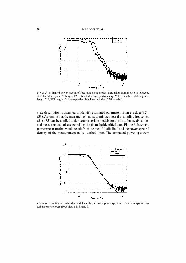
Using the same data that was used to estimate the power spectra in Figure 5,disturbance models are shown for the focus mode in Figure 6. A second-order


Figure 5. Estimated power spectra of focus and coma modes. Data taken from the 3.5 m telescopeat Calar Alto, Spain, 26 May 2002. Estimated power spectra using Welch’s method (data segmentlength 512, FFT length 1024 zero padded, Blackman window, 25% overlap).

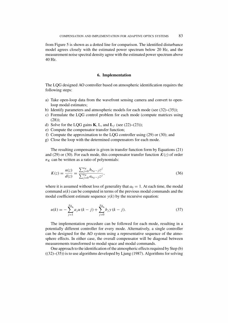
state description is assumed to identify estimated parameters from the data (32)–(33). Assuming that the measurement noise dominates near the sampling frequency,(34)–(35) can be applied to derive appropriate models for the disturbance dynamicsand measurement noise spectral density from the identified data. Figure 6 shows thepower spectrum that would result from the model (solid line) and the power spectraldensity of the measurement noise (dashed line). The estimated power spectrum

Figure 6. Identified second-order model and the estimated power spectrum of the atmospheric dis-turbance to the focus mode shown in Figure 5.


from Figure 5 is shown as a dotted line for comparison. The identified disturbancemodel agrees closely with the estimated power spectrum below 20 Hz, and themeasurement noise spectral density agree with the estimated power spectrum above40 Hz.

6. Implementation

The LQG designed AO controller based on atmospheric identification requires thefollowing steps:

a) Take open-loop data from the wavefront sensing camera and convert to open-loop modal estimates;

b) Identify parameters and atmospheric models for each mode (see (32)–(35));c) Formulate the LQG control problem for each mode (compute matrices using

(28));d) Solve for the LQG gains K, L, and L f (see (22)–(23));e) Compute the compensator transfer function;f) Compute the approximation to the LQG controller using (29) or (30); andg) Close the loop with the determined compensators for each mode.

The resulting compensator is given in transfer function form by Equations (21)and (29) or (30). For each mode, this compensator transfer function K (z) of ordernK can be written as a ratio of polynomials:

K (z) = n(z)

d(z)=

∑nKj=0 bnK − j z j∑nKj=0 anK − j z j

, (36)

where it is assumed without loss of generality that a0 = 1. At each time, the modalcommand u(k) can be computed in terms of the previous modal commands and themodal coefficient estimate sequence y(k) by the recursive equation:

u(k) = −nK∑j=1

a j u (k − j) +nK∑j=0

b j y (k − j). (37)

The implementation procedure can be followed for each mode, resulting in apotentially different controller for every mode. Alternatively, a single controllercan be designed for the AO system using a representative sequence of the atmo-sphere effects. In either case, the overall compensator will be diagonal betweenmeasurements transformed to modal space and modal commands.

One approach to the identification of the atmospheric effects required by Step (b)((32)–(35)) is to use algorithms developed by Ljung (1987). Algorithms for solving


AREs and for determining the controllers based on those solutions as requiredby (d)–(e) ((22)–(23)) are described in many textbooks (Kwakernaak and Sivan,1972; Anderson and Moore, 1990) and implemented in many software packages(MATLAB, 1996).

7. Comparison of performance

The LQG control design procedure described in the preceding sections was testedon a simulation developed by ESO of the MACAO AO system (Donaldson et al.,2000) implemented on the Very Large Telescope (VLT) in Paranal, Chile. TheMACAO has a curvature sensor operating at 350 HZ with 60 subapertures, and abimorph deformable mirror. The simulation represents the controller with a modaldecomposition using the system modes of the MACAO hardware, with the injectionmatrix M = I and nc = 60 (i.e., the “modes” are the voltages of the 60 DM actuators).

The simulation uses a magnitude 14 guidestar within the AO loop. One secondof simulation time will be used to evaluate the AO control algorithm performance.

The same LQG controller will be applied to all modes. The simulation of theMACAO AO system and the MACAO system itself apply the same control algo-rithm to all modes. An integral compensation algorithm with different gains hasnot been developed. If different LQG designs were used for each mode, it would beimpossible to determine whether an observed improvement were due to the LQGdesign methodology or due to the use of individual modal controllers. However,this does not limit the ability of this simulation to illustrate the use of the LQGdesign technique and its performance relative to the standard integral controller.The advantages of applying different optimized controllers to each mode applyequally to any type of controller. The use of a single controller for all modes allowsa simpler, more direct analysis.

The first system mode (which contains the most effective control/sensor pairing)was used in Step (b) of the design procedure. The mirror and actuator dynamicswere assumed to be negligible, but there was assumed to be a computational delayof 0.001 seconds (resulting in two plant states per mode). The algorithm to computethe LQG controller was implemented in Matlab for the MACAO simulation. Thecomputation of single set of controller parameters took about 0.1 sec on a 1 GHzPC operating under Windows 2000.

For this simulation, a three layer model is used with wind speeds of 5.7 m s−1

at 0◦ with weight 0.2, 5.7 m s−1 at 90◦ with weight 0.6 and 33 m s−1 at 0◦ withweight 0.2. The Fried parameter (r0) is 0.1 m. The phase screens for each layer areKolmogorov with an outer scale large enough to have little impact on the validityof the Kolmogorov assumption.

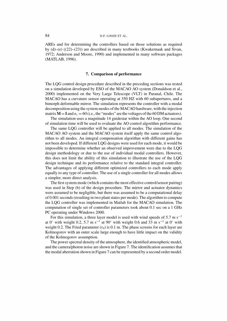
The power spectral density of the atmosphere, the identified atmospheric model,and the camera/photon noise are shown in Figure 7. The identification assumes thatthe modal aberration shown in Figure 7 can be represented by a second order model.


Figure 7. Identified second-order model and the estimated power spectrum of the atmospheric dis-turbance for mode 1 of the MACAO simulation (magnitude 14).

The model transfer function and measurement noise are:

Gd(z) = 1.6381(z + 1) (z − 0.7838)

(z − 0.9476) (z − 0.8357) = 66.9170 (38)

The transfer function of the resulting approximation to the LQG solution is:

KL QG(z) = 0.27401z (z − 0.8022) (z + 0.2079)

(z − 1) (z − 0.8357) (z + 0.0562). (39)

The nominal controller for the MACAO is an integral controller which is iden-tical for all modes and has a gain of 0.4 for this guidestar magnitude. The gain of0.4 produces the best results (in terms of the integrated Strehl—the Strehl ratio forthe image produced by the integrated light—at 1 s and 2.2 µm) to within ±0.05.The transfer function of the nominal controller is:

Kint(z) = 0.4z

z − 1(40)

Both the LQG transfer function (39) and the nominal integral controller (40)can be implemented in the time domain via (36)–(37). The implementation of theLQG controller is:

u(k) = 1.779u(k − 1) − 0.7325 u (k − 2) − 0.04697 u (k − 3)

+ 0.274y(k) − 0.1628y(k − 1) − 0.0457y (k − 2) (41)


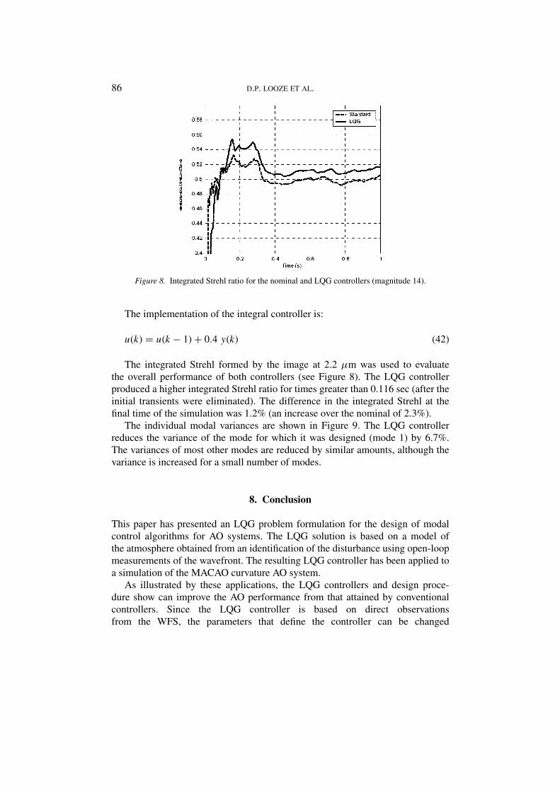
Figure 8. Integrated Strehl ratio for the nominal and LQG controllers (magnitude 14).

The implementation of the integral controller is:

u(k) = u(k − 1) + 0.4 y(k) (42)

The integrated Strehl formed by the image at 2.2 µm was used to evaluatethe overall performance of both controllers (see Figure 8). The LQG controllerproduced a higher integrated Strehl ratio for times greater than 0.116 sec (after theinitial transients were eliminated). The difference in the integrated Strehl at thefinal time of the simulation was 1.2% (an increase over the nominal of 2.3%).

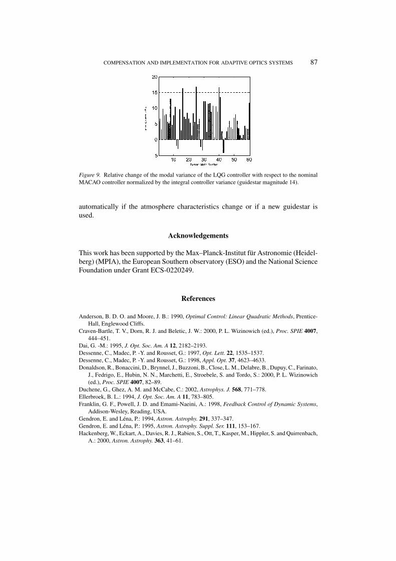
The individual modal variances are shown in Figure 9. The LQG controllerreduces the variance of the mode for which it was designed (mode 1) by 6.7%.The variances of most other modes are reduced by similar amounts, although thevariance is increased for a small number of modes.

8. Conclusion

This paper has presented an LQG problem formulation for the design of modalcontrol algorithms for AO systems. The LQG solution is based on a model ofthe atmosphere obtained from an identification of the disturbance using open-loopmeasurements of the wavefront. The resulting LQG controller has been applied toa simulation of the MACAO curvature AO system.

As illustrated by these applications, the LQG controllers and design proce-dure show can improve the AO performance from that attained by conventionalcontrollers. Since the LQG controller is based on direct observationsfrom the WFS, the parameters that define the controller can be changed


Figure 9. Relative change of the modal variance of the LQG controller with respect to the nominalMACAO controller normalized by the integral controller variance (guidestar magnitude 14).

automatically if the atmosphere characteristics change or if a new guidestar isused.

Acknowledgements

This work has been supported by the Max–Planck-Institut fur Astronomie (Heidel-berg) (MPIA), the European Southern observatory (ESO) and the National ScienceFoundation under Grant ECS-0220249.

References

Anderson, B. D. O. and Moore, J. B.: 1990, Optimal Control: Linear Quadratic Methods, Prentice-Hall, Englewood Cliffs.

Craven-Bartle, T. V., Dorn, R. J. and Beletic, J. W.: 2000, P. L. Wizinowich (ed.), Proc. SPIE 4007,444–451.

Dai, G. -M.: 1995, J. Opt. Soc. Am. A 12, 2182–2193.Dessenne, C., Madec, P. -Y. and Rousset, G.: 1997, Opt. Lett. 22, 1535–1537.Dessenne, C., Madec, P. -Y. and Rousset, G.: 1998, Appl. Opt. 37, 4623–4633.Donaldson, R., Bonaccini, D., Brynnel, J., Buzzoni, B., Close, L. M., Delabre, B., Dupuy, C., Farinato,

J., Fedrigo, E., Hubin, N. N., Marchetti, E., Stroebele, S. and Tordo, S.: 2000, P. L. Wizinowich(ed.), Proc. SPIE 4007, 82–89.

Duchene, G., Ghez, A. M. and McCabe, C.: 2002, Astrophys. J. 568, 771–778.Ellerbroek, B. L.: 1994, J. Opt. Soc. Am. A 11, 783–805.Franklin, G. F., Powell, J. D. and Emami-Naeini, A.: 1998, Feedback Control of Dynamic Systems,

Addison-Wesley, Reading, USA.Gendron, E. and Lena, P.: 1994, Astron. Astrophy. 291, 337–347.Gendron, E. and Lena, P.: 1995, Astron. Astrophy. Suppl. Ser. 111, 153–167.Hackenberg, W., Eckart, A., Davies, R. J., Rabien, S., Ott, T., Kasper, M., Hippler, S. and Quirrenbach,

A.: 2000, Astron. Astrophy. 363, 41–61.


Kasper, M. E.: 2000, Optimization of an Adaptive Optics System and its Application to High-ResolutionImaging Spectroscopy of T Tauri. Ph.D. Thesis, University of Heidelberg, Germany.

Kokotovic, P. K.: 1972, in J. B. Cruz, Jr (ed.), Feedback Systems, McGraw–Hill, New York, 99–137.Kwakernaak, H. and Sivan, R.: 1972, Linear Optimal Control Systems, Wiley-Interscience, New York.Law, N. F. and Lane, R. G.: 1996, Opt. Commun. 126, 19–24.Ljung, L.: 1987, System Identification: Theory for the User, Prentice-Hall, Englewood Cliffs, USA.MATLAB: 1996, MATLAB: Control System Toolbox, The Mathworks, Natick, USA.Noll, R. -J.: 1976. J. Opt. Soc. Am. 66, 207–211.Paschall, R. N. and Anderson, D. J.: 1993, Appl. Opt. 32, 6347–6358.Phillips, R. G.: 1980, Int. J. Control 31, 765–780.Roddier, C., Roddier, F., Northcott, J. E., Graves, J. E. and Jim, K.: 1996, Astrophy. J. 463, 326–335.Roddier, F.: 1988, Appl. Opt. 27, 1223–1225.Sannuti, P. and Kokotovic, P. K.: 1969, IEEE Trans. Autom. Control AC-14, 15–21.Tatarski, V.I.: 1961, R. A. Silverman (translation), Wave Propagation in a Turbulent Medium, Dover

Publications, New York.Tyson, R.K.: 1991, Principles of Adaptive Optics, Academic Press, San Diego.Veran, J. -P., Rigaut, F., Maitre, H. and Rouan, D.: 1997, J. Opt. Soc. Am. A 14, 3057.Wallner, E. P.: 1983, J. Opt. Soc. Am. A 73, 1771–1776.Wild, W. J.: 1996, Opt. Lett. 21, 1433–1435.Wirth, A., Navetta, J., Looze, D. P., Hippler, S., Glindemann, A. and Hamilton, D. : 1998, Appl. Opt.

37, 4586–4597.

Optimal Compensation and Implementation for Adaptive Optics Systems

Documents