Optimal and Hierarchical Controls in Dynamic Stochastic Manufacturing Systems: A Survey S. P. Sethi, H. Yan, H. Zhang, and Q. Zhang School of Management, The University of Texas at Dallas Richardson, TX 75083-0688, USA [email protected] School of Management, The University of Texas at Dallas Richardson, TX 75083-0688, USA [email protected] Institute of Applied Mathematics Academia Sinica, Beijing, 100080, China [email protected] and Department of Mathematics University of Georgia, Athens, GA 30602, USA [email protected] Abstract Most manufacturing systems are large and complex and operate in an uncertain environment. One approach to managing such systems is that of hierarchical decomposition. This paper reviews the research devoted to proving that a hierarchy based on the frequencies of occurrence of different types of events in the systems results in decisions that are asymptotically optimal as the rates of some events become large compared to those of others. The paper also reviews the research on stochas- tic optimal control problems associated with manufacturing systems, their dynamic programming equations, existence of solutions of these equations, and verification theorems of optimality for the systems. Manufacturing systems that are addressed include single machine systems, dynamic flowshops, and dynamic jobshops producing multiple products. These systems may also incorpo- rate random production capacity and demands, and decisions such as production rates, capacity expansion, and promotional campaigns. Related computational results and areas of applications are also presented.

Welcome message from author
This document is posted to help you gain knowledge. Please leave a comment to let me know what you think about it! Share it to your friends and learn new things together.
Transcript
Optimal and Hierarchical Controls in Dynamic Stochastic
Manufacturing Systems: A Survey
S. P. Sethi, H. Yan, H. Zhang, and Q. Zhang
School of Management, The University of Texas at DallasRichardson, TX 75083-0688, USA
School of Management, The University of Texas at DallasRichardson, TX 75083-0688, USA
Institute of Applied MathematicsAcademia Sinica, Beijing, 100080, China
andDepartment of Mathematics
University of Georgia, Athens, GA 30602, [email protected]
Abstract
Most manufacturing systems are large and complex and operate in an uncertain environment. Oneapproach to managing such systems is that of hierarchical decomposition. This paper reviews theresearch devoted to proving that a hierarchy based on the frequencies of occurrence of different typesof events in the systems results in decisions that are asymptotically optimal as the rates of someevents become large compared to those of others. The paper also reviews the research on stochas-tic optimal control problems associated with manufacturing systems, their dynamic programmingequations, existence of solutions of these equations, and verification theorems of optimality forthe systems. Manufacturing systems that are addressed include single machine systems, dynamicflowshops, and dynamic jobshops producing multiple products. These systems may also incorpo-rate random production capacity and demands, and decisions such as production rates, capacityexpansion, and promotional campaigns. Related computational results and areas of applicationsare also presented.
Table of Contents
1. Introduction.
2. Optimal Control with the Discounted Cost Criterion.
2.1 Single or parallel machine systems
2.2 Dynamic flowshops
2.3 Dynamic jobshops
3. Hierarchical Controls with the Discounted Cost Criterion
3.1 Single or parallel machine systems
3.2 Dynamic flowshops
3.3 Dynamic jobshops
3.4 Computational results
3.5 Production-investment models
3.6 Other multilevel models
3.7 Single or parallel machine systems with the risk-sensitive discounted cost criterion
4. Optimal Controls with the Long-Run Average Cost Criterion
4.1 Single or parallel machine systems
4.2 Dynamic flowshops
4.3 Dynamic jobshops
5. Hierarchical Controls with the Long-Run Average Cost Criterion
5.1 Single or parallel machine systems
5.2 Dynamic flowshops
5.3 Dynamic jobshops
5.4 Markov decision processes with weak and strong interactions
5.5 Single or parallel machine systems with the risk-sensitive average cost criterion
6. Extensions and Concluding Remarks
1
1 Introduction
Most manufacturing firms are large, complex systems characterized by several decision subsystems,
such as finance, personnel, marketing, and operations. They may have a number of plants and
warehouses, and they produce a large number of different products using a wide variety of machines
and equipment. Moreover, these systems are subject to discrete events such as construction of new
facilities, purchase of new equipment and scrappage of old, machine setups, failures, and repairs,
and new product introductions. These events could be deterministic or stochastic. Management
must recognize and react to these events. Because of the large size of these systems and the
presence of these events, obtaining exact optimal policies to run these systems is nearly impossible
both theoretically and computationally.
One way to cope with these complexities is to develop methods of hierarchical decision making
for these systems. The idea is to reduce the overall complex problem into manageable approximate
problems or subproblems, to solve these problems, and to construct a solution for the original
problem from the solutions of these simpler problems.
There are several different (and not mutually exclusive) ways by which to reduce the complex-
ity. These include decomposing the problem into problems of smaller subsystems with a proper
coordinating mechanism; aggregating products and subsequently disaggregating them; replacing
random processes with their averages and possibly other moments; modeling uncertainties in the
production planning problem via diffusion processes; and so on. Development of such approaches
for large, complex systems was identified as a particular fruitful research area by the Committee
on the Next Decade in Operations Research (1988), as well as by the Panel on Future Directions
in Control Theory chaired by Fleming (1988). A great deal of research has been conducted in the
areas of Operations Research, Operations Management, Systems Theory, and Control Theory. For
their importance in practice, see the surveys of the literature by Libosvar (1988), Rogers et al.
(1991), Bitran and Tirupati (1993), and Cheng (1999), a bibliography complied by Bukh (1992),
and books by Stadtler (1988) and Switalski (1989). Some other references on hierarchical systems
are Simon (1962), Mesarovic et al. (1970), Smith and Sage (1973), Singh (1982), Saksena et al.
(1984), and Auger (1989). It should be noted, however, that most of them concern deterministic
systems.
2
Each approach mentioned above is suited to certain types of models and assumptions. The
approach we shall first discuss is that of modeling uncertainties in the production planning problem
via diffusion processes. The idea is initiated by Sethi and Thompson (1981a, b) and Bensoussan et
al. (1984). Because controlled diffusion problems can often be solved (see Ghosh et al. (1993, 1997),
Harrison and Taksar (1983), and Harrison et al. (1983)), one uses the controlled diffusion models to
approximate stochastic manufacturing systems. Kushner and Ramachandran (1989) begin with a
sequence of systems whose limit is a controlled diffusion process. It should be noted that the traffic
intensities of the systems in sequence converge to the critical intensity of one. They show that the
sequence of value functions associated with the given sequence converges to the value function of the
limiting problem. This enables them to construct a sequence of asymptotic optimal policies defined
to be those for which the difference between the associated cost and the value function converges
to zero as the traffic intensity approaches its critical value. The most important application of
this approach concerns the scheduling of networks of queues. If a network of queues is operating
under heavy traffic, that is, when the rate of customers entering some of the stations in the network
is very close to the rate of service at those stations, the problem of scheduling the network can
be approximated by a dynamic control problem involving diffusion processes. The optimal policies
that are obtained for the dynamic control problem involving diffusion approximation are interpreted
in terms of the original problem. A justification of this procedure based on simulation is provided
in Harrison and Wein (1989, 1990), Wein (1990), and Kumar and Kumar (1994), for example;
see also the survey on fluid models and strong approximations by Chen and Mandelbaum (1994).
Furthermore, Krichagina et al. (1993) and Krichagina et al. (1994) apply this approach to the
problem of controlling the production rate of a single product using a single unreliable machine
in order to minimize the total discounted inventory/backlog costs. They imbed the given system
into a sequence of systems in heavy traffic. Their purpose is to obtain asymptotic optimal policies
for the sequence of systems that can be expressed only in terms of the parameters of the original
system.
It should be noted that these approaches do not provide us with an estimate of how much
the policies constructed for the given original system deviate from the optimal solution, especially
when the optimal solution is not known, which is most often the case. As we shall see later,
the hierarchical approach under consideration in this survey enables one to provide just such an
3
estimate in many cases.
The next approach we shall discuss is that of aggregation-disaggregation. Bitran et al. (1986)
formulate a model of a manufacturing system in which uncertainties arise from demand estimates
and forecast revisions. They consider first a two-level product hierarchical structure, which is
characterized by families and items. Hence, the production planning decisions consist of determining
the sequence of the product families and the production lot sizes for items within each family, with
the objective of minimizing the total cost. Then, they consider demand forecasts and forecast
revisions during the planning horizon. The authors assume that the mean demand for each family
is invariant and that the planners can estimate the improvement in the accuracy of forecasts, which
is measured by the standard deviation of forecast errors. Bitran et al. (1986) view the problem
as a two-stage hierarchical production planning problem. The aggregate problem is formulated as
a deterministic mixed integer program that provides a lower bound on the optimal solution. The
solution to this problem determines the set of product families to be produced in each period. The
second-level problem is interpreted as the disaggregate stage where lot sizes are determined for the
individual product to be scheduled in each period. Only a heuristic justification has been provided
for the approach described. Some other references in the area are Bitran and Hax (1977), Hax and
Candea (1984), Gelders and Van Wassenhove (1981), Ari and Axsater (1988), and Nagi (1991).
Lasserre and Merce (1990) assume that the aggregate demand forecast is deterministic, while
the detailed level forecast is nondeterministic within known bounds. Their aim is to obtain an
aggregate plan for which there exists a feasible dynamic disaggregation policy. Such an aggregate
plan is called a robust plan, and they obtain necessary and sufficient conditions for robustness; see
also Gfrerer and Zapfel (1994).
Finally we consider the approach of replacing random processes with their averages and possibly
other moments, see Sethi and Zhang (1994a, 1998) and Sethi et al. (2000e). The idea of the
approach is to derive a limiting control problem which is simpler to solve than the given original
problem. The limiting problem is obtained by replacing the stochastic machine capacity process
by the average total capacity of machines and by appropriately modifying the objective function.
The solution of this problem provides us with longer-term decisions. Furthermore, given these
decisions, there are a number of ways by which we can construct short-term production decisions.
By combining these decisions, we create an approximate solution of the original, more complex
4
problem.
The specific points to be addressed in this review are results on the asymptotic optimality of the
constructed solution and the extent of the deviation of its cost from the optimal cost for the original
problem. The significance of these results for the decision-making hierarchy is that management
at the highest level of the hierarchy can ignore the day-to-day fluctuation in machine capacities, or
more generally, the details of shop floor events, in carrying out long-term planning decisions. The
lower operational level management can then derive approximate optimal policies for running the
actual (stochastic) manufacturing system.
While the approach could be extended for applications in other areas, the purpose here is to
review models of a variety of representative manufacturing systems in which some of the exogenous
processes, deterministic or stochastic, are changing much faster than the remaining ones, and to
apply the methodology of hierarchical decision making to them. We are defining a fast changing
process as a process that is changing so rapidly that from any initial condition, it reaches its
stationary distribution in a time period during which there are few, if any, fluctuations in the other
processes.
In what follows we review applications of the approach to stochastic manufacturing problems,
where the objective function is to minimize a total discounted cost, a long-run average cost, or a
risk-sensitive criterion. We also summarize results on dynamic programming equations, existence of
their solutions, and verification theorems of optimality for single/parallel machine systems, dynamic
flowshops, and dynamic jobshops producing multiple products. Sections 2 and 3 are devoted
to discounted cost models. In Section 2, we review the existence of solutions to the dynamic
programming equations associated with stochastic manufacturing systems with the discounted cost
criterion. The verification theorems of optimality and the characterization of optimal controls are
also given. Section 3 discusses the results on open-loop and/or feedback hierarchical controls that
have been developed and shown to be asymptotically optimal for the systems. The computational
issues are also included in this section. Sections 4 and 5 are devoted to average cost models. In
Section 4, we review the existence of solutions to the ergodic equations corresponding to stochastic
manufacturing systems with the long-run average cost criterion and the corresponding verification
theorems and the characterization of optimal controls. Section 5 surveys hierarchical controls for
single machine systems, flowshops, and jobshops with the long-run average cost criterion or the
5
risk-sensitive long-run average cost criterion. Markov decision processes with weak and strong
interactions are also included. Important insights have been gained from the research reviewed
here, see Sethi (1997). Some of these insights are given where appropriate. Section 6 concludes the
paper.
2 Optimal Control with the Discounted Cost Criterion
The class of convex production planning models is an important paradigm in the operations man-
agement/operations research literature. The earliest formulation of a convex production planning
problem in a discrete-time framework dates back to Modigliani and Hohn (1955). They were inter-
ested in obtaining a production plan over a finite horizon in order to satisfy a deterministic demand
and minimize the total discounted convex costs of production and inventory holding. Since then
the model has been further studied and extended in both continuous-time and discrete-time frame-
works by a number of researchers, including Johnson (1957), Arrow et al.(1958), Veinott (1964),
Adiri and Ben-Israel (1966), Sprzeuzkouski (1967), Lieber (1973), and Hartl and Sethi (1984). A
rigorous formulation of the problem along with a comprehensive discussion of the relevant literature
appears in Bensoussan et al.(1983).
Extensions of the convex production planning problem to incorporate stochastic demand have
been analyzed mostly in the discrete-time framework. A rigorous analysis of the stochastic problem
has been carried out in Bensoussan et al. (1983). Continuous-time versions of the model that
incorporate additive white noise terms in the dynamics of the inventory process were analyzed by
Sethi and Thompson (1981a) and Bensoussan et al. (1984).
Earlier works that relate most closely to problems under consideration here include Kimemia
and Gershwin (1983), Akella and Kumar (1986), Fleming et al. (1987), Sethi et al. (1992a), and
Lehoczky et al. (1991). These works incorporate piecewise deterministic processes (PDP) either in
the dynamics or in the constraints of the model. Fleming et al. (1987) consider the demand to be
a finite state Markov process. In the models of Kimemia and Gershwin (1983), Akella and Kumar
(1986), Sethi et al. (1992a) and Lehoczky et al. (1991), the production capacity rather than the
demand for production is modeled as a stochastic process. In particular, the process of machine
breakdown and repair is modeled as a birth-death process, thus making the production capacity
over time a finite state Markov process. Feng and Yan (2000) incorporate a Markovian demand in
6
a discrete state version of the model of Akella and Kumar (1986).
Here we will discuss the optimality of single/parallel machine systems, N -machine flowshops,
and general jobshops.
2.1 Single or parallel machine systems
Akella and Kumar (1986) deal with a single machine (with two states: up and down), single
product problem. They obtained an explicit solution for the threshold inventory level, in terms
of which the optimal policy is as follows: Whenever the machine is up, produce at the maximum
possible rate if the inventory level is less than the threshold, produce on demand if the inventory
level is exactly equal to the threshold, and not produce at all if the inventory level exceeds the
threshold. When their problem is generalized to convex costs and more than two machine states,
it is no longer possible to obtain an explicit solution. Using the viscosity solution technique, Sethi
et al. (1992a) investigate this general problem. They study the elementary properties of the value
function. They show that the value function is a convex function, and that it is strictly convex
provided the inventory cost is strictly convex. Moreover, it is shown to be a viscosity solution
to the Hamilton-Jacobi-Bellman (HJB) equation and to have upper and lower bounds each with
polynomial growth. Following the idea of Thompson and Sethi (1980), they define what are known
as the turnpike sets in terms of the corresponding value function. They prove that the turnpike
sets are attractors for the optimal trajectories and provide sufficient conditions under which the
optimal trajectories enter the convex closure in finite time. Also, they give conditions to ensure
that the turnpike sets are non-empty.
To more precisely state their results, we need to specify the model of a single/parallel ma-
chine manufacturing system. Let x(t), u(t), z, and m(t) denote, respectively, the surplus (inven-
tory/shortage) level, the production rate, the demand rate, and the machine capacity level at time
t ∈ [0,∞). We assume shortages to be backlogged. Here and throughout the paper, vectors will
be denoted by bold-faced letters. We assume that x(t) ∈ Rn, u(t) ∈ Rn+, (i.e., u(t) ≥ 0), and z is
a constant positive vector in Rn+. Furthermore, we assume that m(·) is a Markov process with a
finite space M = 0, 1, ..., p. We can now write the dynamics of the system as
x(t) = u(t)− z, x(0) = x. (2.1)
Definition 2.1. A control process (production rate) u(·) = u(t) : t ≥ 0 is called admissible
7
with respect to the initial capacity m if (i) u(·) is history-dependent or, more precisely, adapted
to the filtration Ft : t ≥ 0 with Ft = σm(s) : 0 ≤ s ≤ t, the σ-field generated by m(t);
(ii) 0 ≤ 〈r,u(t)〉 ≤ m(t) for all t ≥ 0 for some positive vector r, where 〈·, ·〉 between r and u(t)
represents inner product of vectors r and u(t).
Let A(m) denote the set of all admissible control processes with the initial condition m(0) = m.
Definition 2.2. A real-valued function u(x,m) on Rn ×M is called an admissible feedback
control, or simply a feedback control, if (i) for any given initial x, the equation x(t) = u(x(t),m(t))−z, x(0) = x, has a unique solution; (ii) u(·) = u(t) = u(x(t),m(t)) : t ≥ 0 ∈ A(m).
Let h(x) and c(u) denote the surplus cost and the production cost functions, respectively. For
every u(·) ∈ A(m), x(0) = x, and m(0) = m, define the cost criterion
J(x,m, u(·)) = E
∫ ∞
0e−ρt[h(x(t)) + c(u(t))]dt, (2.2)
where ρ > 0 is the given discount rate. The problem is to choose an admissible control u(·) that
minimizes J(x,m, u(·)). We define the value function as
v(x,m) = infu(·)∈A(m)
J(x,m, u(·)). (2.3)
We make the following assumptions on the cost functions h(x) and c(u).
(A.2.1) h(x) is nonnegative and convex with h(0) = 0. There are positive constants C21, C22, C23,
κ21 ≥ 0, and κ22 ≥ 0 such that C21|x|κ21 − C22 ≤ h(x) ≤ C23(1 + |x|κ22).
(A.2.2) c(u) is nonnegative, c(0) = 0, and c(u) is twice differentiable. Moreover, c(u) is either strictly
convex or linear.
(A.2.3) m(·) is a finite state Markov chain with generator Q, where Q = (qij), i, j ∈M is a (p + 1)×(p + 1) matrix such that qij ≥ 0 for i 6= j and qii = −∑
i6=j qij . That is, for any function f(·)on M,
Qf(·)(m) =∑
6=m
qm`[f(`)− f(m)].
With these three assumptions we can state the following theorem concerning the properties of the
value function v(·, ·), proved in Fleming et al. (1987).
Theorem 2.1. (i) For each m, v(·,m) is convex on Rn, and v(·,m) is strictly convex if h(·) is
so; (ii) There exist positive constants C24, C25, and C26 such that for each m, C24|x|κ21 − C25 ≤v(x,m) ≤ C26(1 + |x|κ22).
8
We next consider the HJB equation associated with the problem. Let F (m,w) = inf〈u−z, w〉 :
0 ≤ 〈u, r〉 ≤ m, where r is given in Definition 2.1. Then, the HJB equation is written formally as
follows:
ρv(x,m) = F (m, v′x(x,m)) + h(x) + Qv(x, ·)(m), (2.4)
for x ∈ Rn, m ∈M, where v′x(x,m) is the partial derivative (gradient) of v(·, ·) with respect to x.
In general, the value function v(x,m) may not be differentiable. In order to make sense of the
HJB equation (2.4), we consider its viscosity solution, see Fleming and Soner (1992). To define
a viscosity solution, we first introduce the superdifferential and subdifferential of a given function
f(x) on Rn.
Definition 2.3. The superdifferential D+f(x) and the subdifferential D−f(x) of any function
f(x) on Rn are defined, respectively, as follows:
D+f(x) =
s ∈ Rn : lim sup
|r|→0
f(x + r)− f(x)− 〈r, s〉|r| ≤ 0
,
D−f(x) =
s ∈ Rn : lim inf
|r|→0
f(x + r)− f(x)− 〈r, s〉|r| ≥ 0
.
Definition 2.4. We say that v(x,m) is a viscosity solution of equation (2.4) if the following
holds: (i) v(x,m) is continuous in x and there exist C27 > 0 and κ23 > 0 such that |v(x, m)| ≤C27(1 + |x|κ23); (ii) for all n ∈ D+v(x,m), ρv(x,m) − F (m, v′x(x,m)) + h(x) + Qv(x, ·)(m) ≤ 0;
and (iii) for all n ∈ D−v(x,m), ρv(x,m)− F (m, v′x(x,m)) + h(x) + Qv(x, ·)(m) ≥ 0.
Lehoczky et al. (1991) prove the following theorem.
Theorem 2.2. The value function v(x,m) defined in (2.3) is the unique viscosity solution to
the HJB equation (2.4).
Remark 2.1. If there is a continuously differentiable function that satisfies the HJB equation
(2.4), then it is a viscosity solution, and therefore, it is the value function. Furthermore, we have
the following result.
Theorem 2.3. The value function v(·,m) is continuously differentiable and satisfies the HJB
equation (2.4).
For its proof, see Theorem 3.1 in Sethi and Zhang (1994a). Next, we give a verification theorem.
Theorem 2.4. (Verification Theorem) Suppose that there is a continuously differentiable func-
tion v(x,m) that satisfies the HJB equation (2.4). If there exists u∗(·) ∈ A(m), for which the
9
corresponding x∗(t) satisfies (2.1) with x∗(0) = x, w∗(t) = v′x(x∗(t),m(t)), and F (m(t), w∗(t)) =
〈u∗(t) − z,w∗(t)〉 + c(u∗(t)), almost everywhere in t with probability one, then v(x,m) = v(x,m)
and u∗(t) is optimal, i.e., v(x, m) = v(x,m) = J(x,m, u∗(·)).For its proof, see Lemma H.3 of Sethi and Zhang (1994a). We now give an application of the
verification theorem. With Assumption (A.2.2), we can use the verification theorem to derive an
optimal feedback control for n = 1. From Theorem 2.4, an optimal feedback control u∗(x,m) must
minimize (u− z)v′x(x,m) + c(u). Thus,
u∗(x,m) =
0 if v′x(x,m) ≥ 0
(c)−1(−v′x(x,m)) if − c(m) ≤ v′x(x,m) < 0
m if v′x(x,m) < −c(m),
when the second derivative of c(u) is strictly positive, and
u∗(x, m) =
0 if v′x(x,m) > −c
minz, m if v′x(x,m) = −c
m if v′x(x,m) < −c,
when c(u) = cu for some constant c ≥ 0.
Recall that v(·,m) is a convex function. Thus, u∗(x, m) is increasing in x. From a result on
differential equations (see Hartman (1982)), x(t) = u∗(x(t),m(t)) − z, x(0) = x, has a unique
solution x∗(t) for each sample path of the capacity process. Hence, the control given above is the
optimal feedback control. From this application, we can see that the points satisfying v′x(x,m) =
−c(z) are critical in describing the optimal feedback control. So we give the following definition.
Definition 2.5. The turnpike set G(m, z) is defined by G(m, z) = x ∈ R : v′x(x,m) = −c(z).Next we will discuss the monotonicity of the turnpike set. To do this, define i0 ∈M to be such
that i0 < z < i0 + 1. Observe that for m ≤ i0, x(t) ≤ m − z ≤ i0 − z < 0. Therefore, x(t) goes to
−∞ monotonically as t →∞, if the capacity state m is absorbing. Hence, only those m ∈ M, for
which m ≥ i0 + 1, are of special interest to us.
In view of Theorem 2.1, if h(·) is strictly convex, then each turnpike set reduces to a singleton,
i.e., there exists an xm such that G(m, z) = xm, m ∈ M. If the production cost is linear, i.e.,
c(u) = cu for some constant c, then xm is the threshold inventory level with capacity m. Specifically,
if x > xm, u∗(x,m) = 0, and if x < xm, u∗(x,m) = m (full available capacity).
10
Let us make the following observation. If the capacity m > z, then the optimal trajectory
will move toward the turnpike set xm. Suppose the inventory level is xm for some m and the
capacity increases to m1 > m; it then becomes costly to keep the inventory at level xm, since a
lower inventory level may be more desirable given the higher current capacity. Thus, we expect
xm1 ≤ xm. Sethi et al. (1992a) show that this intuitive observation is true. We state their result
as the following theorem.
Theorem 2.5. Assume h(·) to be differentiable and strictly convex. Then xi0 ≥ xi0+1 ≥ · · · ≥xm ≥ cz, where cz = (h)−1(−ρc(z)).
2.2 Dynamic flowshops
We consider a dynamic flowshop that produces a single finished product using N machines in
tandem that are subject to breakdown and repair. In comparison to the single/parallel machine
systems, the flowshop problem with internal buffers and the resulting state constraints is much
more complicated. Certain boundary conditions need to be taken into account for the associated
HJB equation, see Soner (1986). Optimal control policy can no longer be described simply in terms
of some hedging points. Lou et al. (1994) show that the optimal control policy for a two-machine
flowshop with linear costs of production can be given in terms of two switching manifolds. However,
the switching manifolds are not easy to obtain. One way to compute them is to approximate them
by continuous piecewise-linear functions as done by Van Ryzin et al. (1993), in the absence of
production costs. To rigorously deal with the general flowshop problem under consideration, the
HJB equation in terms of the directional derivatives (HJBDD) at inner and boundary points are
introduced by Presman et al. (1993, 1995). They show that the value function corresponding to the
dynamic flowshop problem is a solution of the HJBDD equation. They also establish a verification
theorem. Presman et al. (1997b) extend these results to dynamic flowshops with limited buffers.
Because dynamic flowshops are special cases of dynamic jobshops reviewed in detail in the next
section, we will not discuss them in detail here separately.
2.3 Dynamic jobshops
Consider a manufacturing system producing a variety of products in demand using machines in a
general network configuration, which generalizes both the parallel and the tandem machine models.
Each product follows a process plan—possibly from a number of alternative process plans—that
11
specifies the sequence of machines it must visit and the operations performed by them. A process
plan may call for multiple visits to a given machine, as is the case in semiconductor manufacturing;
Lou and Kager (1989), Srivatsan et al. (1994), Uzsoy et al. (1996), and Yan et al. (1994, 1996).
Often the machines are unreliable. Over time they break down and must be repaired. A manu-
facturing system so described will be termed a dynamic jobshop. Now we give the mathematically
description of a jobshop suggested by Presman et al. (1997a), as a revision of the description by
Sethi and Zhou (1994). First we give some definitions.
Definition 2.6. A manufacturing digraph is a graph (∆, Π), where ∆ is a set of Nb + 2 (≥ 3),
vertices, and Π is a set of ordered pairs called arcs, satisfying the following properties: (i) there is
only one source, labeled 0, and only one sink, labeled Nb + 1, in the digraph; (ii) no vertex in the
graph is isolated; and (iii) the digraph does not contain any cycle.
Remark 2.2. Condition (ii) is not an essential restriction. Inclusion of isolated vertices is
merely a nuisance. This is because an isolated vertex is like a warehouse that can only ship out
parts of a particular type to meet their demand. Since no machine (or production) is involved,
its inclusion or exclusion does not affect the optimization problem under consideration. Condition
(iii) is imposed to rule out the following two trivial situations: (a) a part of type i in buffer i gets
processed on a machine without any transformation and returns to buffer i, and (b) a part of type
i is processed and converted back into a part of type j, j 6= i, and is then processed further on a
number of machines to be converted back into a part of type i. Moreover, if we had included any
cycle in our manufacturing system, the flow of parts that leave buffer i only to return to buffer i
would be zero in any optimal solution. It is unnecessary, therefore, to complicate the problem by
including cycles.
Definition 2.7. In a manufacturing digraph, the source is called the supply node and the sink
represents the customers. Vertices immediately preceding the sink are called external buffers, and
all others are called internal buffers.
In order to obtain the system dynamics from a given manufacturing digraph, a systematic
procedure is required to label the state and control variables. For this purpose, note that our
manufacturing digraph (∆,Π) contains a total of Nb + 2 vertices including the source, the sink, d
internal buffers, and Nb − d external buffers for some integer d and Nb, 0 ≤ d ≤ Nb − 1, Nb ≥ 1.
The proof of the following theorem is similar to Theorem 2.2 in Sethi and Zhou (1994).
12
Theorem 2.6. We can label all the vertices from 0 to Nb +1 in a way so that the label numbers
of the vertices along every path are in a strictly increasing order, that is, the source is labeled 0,
the sink is labeled Nb + 1, and the external buffers are labeled d + 1, d + 2, ..., Nb.
Definition 2.8. For each arc (i, j), j 6= Nb + 1, in a manufacturing digraph, the rate at which
parts in buffer i are converted to parts in buffer j is labeled as control uij . Moreover, the control
uij associated with the arc (i, j) is called an output of i and an input to j. In particular, outputs
of the source are called primary controls of the digraph. For each arc (i, Nb + 1), i = d + 1, ..., Nb,
the demand for products in buffer i is denoted by zi.
In what follows, we shall also set
ui,Nb+1 = zi, i = d + 1, ..., Nb,
ui,j = 0, for (i, j) 6∈ Π, 0 ≤ i ≤ Nb and 1 ≤ j ≤ Nb + 1,
for a unified notation suggested in Presman et al. (1997a). While zi and ui,j for (i, j) 6∈ Π are not
controls, we shall for convenience refer to ui,j , 0 ≤ i ≤ Nb, 0 ≤ j ≤ Nb +1, as controls. In this way,
we can consider the controls as an (Nb + 1)× (Nb + 1) matrix u = (uij) of the following form:
u0,1 u0,2 ... u0,i u0,i+1 ... u0,d u0,d+1 ... u0,Nb−1 u0,Nb0
0 u1,2 ... u1,i u1,i+1 ... u1,d u1,d+1 ... u1,Nb−1 u1,Nb0
... ... ... ... ... ... ... ... ... ... ... ...
0 0 ... ui−1,i ui−1,i+1 ... ui−1,d ui−1,d+1 ... ui−1,Nb−1 ui−1,Nb
0 0 ... 0 ui,i+1 ... ui,d ui,d+1 ... ui,Nb−1 ui,Nb0
... ... ... ... ... ... ... ... ... ... ... ...
0 0 ... 0 0 ... ud−1,d ud−1,d+1 ... ud−1,Nb−1 ud−1,Nb0
0 0 ... 0 0 ... 0 ud,d+1 ... ud,Nb−1 ud,Nb0
0 0 ... 0 0 ... 0 0 ... 0 0 ud+1,Nb+1
... ... ... ... ... ... ... ... ... ... ... ...
0 0 ... 0 0 ... 0 0 ... 0 0 uNb,Nb+1
The set of all such controls is written as U , i.e., U = u = (uij) : 0 ≤ i ≤ Nb, 1 ≤ j ≤ Nb +
1, uij = 0 for (i, j) 6∈ Π. Before writing the dynamics and the state constraints corresponding
to the manufacturing digraph (∆, Π) containing Nb + 2 vertices consisting of a source, a sink, d
internal buffers, and Nb−d external buffers associated with the Nb−d distinct final products to be
13
manufactured (or characterizing a jobshop), we give the description of the control constraints. We
label all the vertices according to Theorem 2.8. For simplicity in the sequel, we shall call the buffer
whose label is i as buffer i, i = 1, 2, ..., Nb. The control constraints depend on the placement of
the machines, and the different placements on the same digraph will give rise to different jobshops.
In other words, a jobshop corresponds to a unique digraph, whereas a digraph may correspond to
many different jobshops. Therefore, to uniquely characterize a jobshop using graph theory, we need
to introduce the concept of a placement of machines, or simply a placement. Let Nb ≤ π−Nb + d,
where π denotes the total number of arcs in Π.
Definition 2.9. In a manufacturing digraph (∆,Π), a set K = K1, K2, ...,KN is called a
placement of machines 1, 2, ..., N , if K is a partition of Π = (i, j) ∈ Π : j 6= Nb + 1, namely,
∅ 6= Kn ⊂ Π, Kn ∩K` = ∅ for n 6= `, and ∪Nk=1Kk = Π.
A dynamic jobshop can be uniquely specified by a triple (∆, Π,K), which denotes a manufactur-
ing system that corresponds to a manufacturing digraph (∆, Π) along with a placement of machines
K = (K1,K2, ..., KN ). Consider a jobshop (∆,Π,K), let uij(t) be the control at time t associated
with arc (i, j), (i, j) ∈ Π. Suppose we are given a stochastic process m(t) = (m1(t), ..., mN (t)) on
the probability space (Ω,F , P ) with mn(t) representing the capacity of the nth machine at time t,
n = 1, ..., N . The controls uij(t) with (i, j) ∈ Kn, n = 1, ..., N , t ≥ 0, should satisfy the following
constraints: 0 ≤ ∑(i,j)∈Kn
uij(t) ≤ mn(t) for all t ≥ 0, n = 1, ..., N, where we have assumed that
the required machine capacity pij (for unit production rate of type j from part type i) equals 1,
for convenience in exposition. The analysis can be readily extended to the case when the required
machine capacity for the unit production rate of part j from part i is any given positive constant.
We denote the surplus at time t in buffer i by xi(t), i ∈ ∆ \ 0, Nb + 1. Note that if xi(t) > 0,
i = 1, ..., Nb, we have an inventory in buffer i, and if xi(t) < 0, i = d + 1, ..., Nb, we have a shortage
of finished product i. The dynamics of the system are, therefore,
xi(t) =(∑i−1
`=0 u`i(t)−∑Nb
`=i+1 ui`(t))
, 1 ≤ i ≤ d,
xi(t) =(∑d
`=0 u`i(t)− zi
), d + 1 ≤ i ≤ Nb,
(2.5)
for some integer d and x(0) := (x1(0), ..., xNb(0)) = (x1, ..., xNb
) = x. Since internal buffers provide
inputs to machines, a fundamental physical fact about them is that they must not have shortages.
14
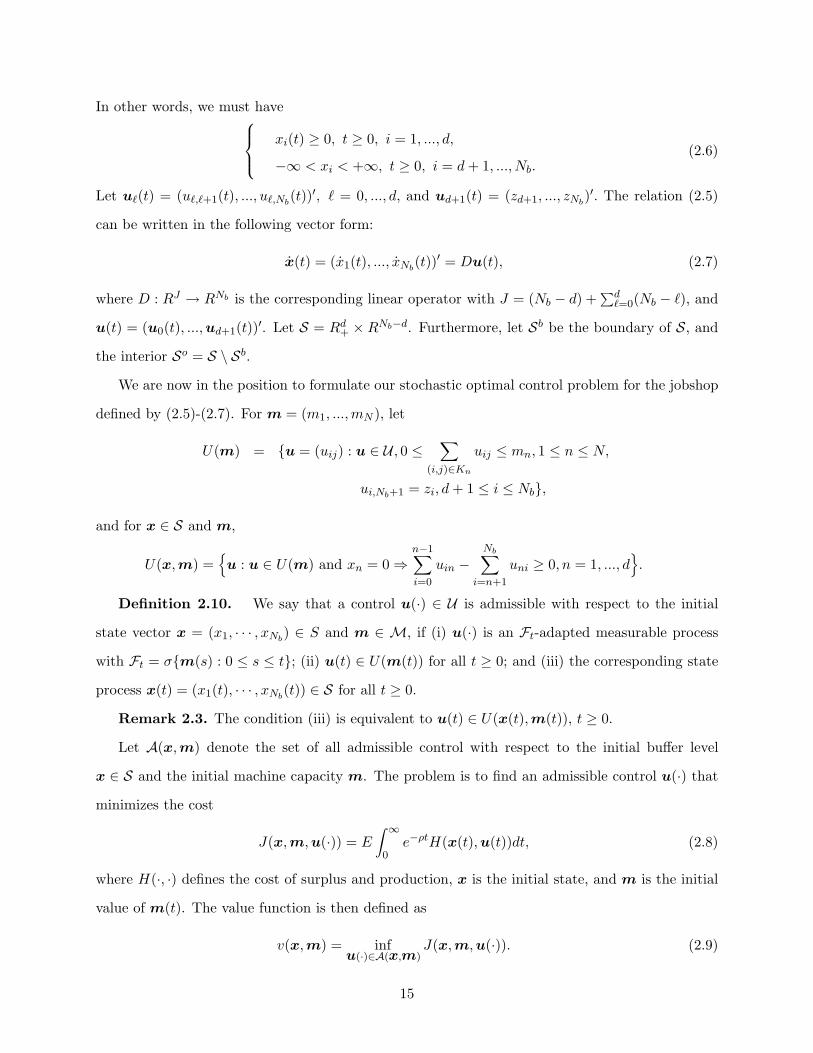
In other words, we must have
xi(t) ≥ 0, t ≥ 0, i = 1, ..., d,
−∞ < xi < +∞, t ≥ 0, i = d + 1, ..., Nb.(2.6)
Let u`(t) = (u`,`+1(t), ..., u`,Nb(t))′, ` = 0, ..., d, and ud+1(t) = (zd+1, ..., zNb
)′. The relation (2.5)
can be written in the following vector form:
x(t) = (x1(t), ..., xNb(t))′ = Du(t), (2.7)
where D : RJ → RNb is the corresponding linear operator with J = (Nb − d) +∑d
`=0(Nb − `), and
u(t) = (u0(t), ...,ud+1(t))′. Let S = Rd+ × RNb−d. Furthermore, let Sb be the boundary of S, and
the interior So = S \ Sb.
We are now in the position to formulate our stochastic optimal control problem for the jobshop
defined by (2.5)-(2.7). For m = (m1, ..., mN ), let
U(m) = u = (uij) : u ∈ U , 0 ≤∑
(i,j)∈Kn
uij ≤ mn, 1 ≤ n ≤ N,
ui,Nb+1 = zi, d + 1 ≤ i ≤ Nb,
and for x ∈ S and m,
U(x,m) =u : u ∈ U(m) and xn = 0 ⇒
n−1∑
i=0
uin −Nb∑
i=n+1
uni ≥ 0, n = 1, ..., d.
Definition 2.10. We say that a control u(·) ∈ U is admissible with respect to the initial
state vector x = (x1, · · · , xNb) ∈ S and m ∈ M, if (i) u(·) is an Ft-adapted measurable process
with Ft = σm(s) : 0 ≤ s ≤ t; (ii) u(t) ∈ U(m(t)) for all t ≥ 0; and (iii) the corresponding state
process x(t) = (x1(t), · · · , xNb(t)) ∈ S for all t ≥ 0.
Remark 2.3. The condition (iii) is equivalent to u(t) ∈ U(x(t), m(t)), t ≥ 0.
Let A(x,m) denote the set of all admissible control with respect to the initial buffer level
x ∈ S and the initial machine capacity m. The problem is to find an admissible control u(·) that
minimizes the cost
J(x, m, u(·)) = E
∫ ∞
0e−ρtH(x(t), u(t))dt, (2.8)
where H(·, ·) defines the cost of surplus and production, x is the initial state, and m is the initial
value of m(t). The value function is then defined as
v(x, m) = infu(·)∈A(x,m)
J(x, m, u(·)). (2.9)
15
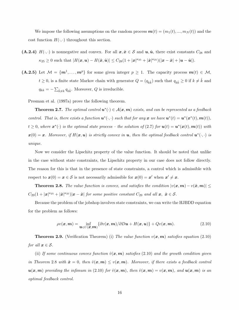
We impose the following assumptions on the random process m(t) = (m1(t), ...,mN (t)) and the
cost function H(·, ·) throughout this section.
(A.2.4) H(·, ·) is nonnegative and convex. For all x, x ∈ S and u, u, there exist constants C28 and
κ25 ≥ 0 such that |H(x, u)−H(x, u)| ≤ C28(1 + |x|κ25 + |x|κ25)(|x− x|+ |u− u|).
(A.2.5) Let M = m1, . . . ,mp for some given integer p ≥ 1. The capacity process m(t) ∈ M,
t ≥ 0, is a finite state Markov chain with generator Q = (qkk) such that qkk ≥ 0 if k 6= k and
qkk = −∑k 6=k qkk. Moreover, Q is irreducible.
Presman et al. (1997a) prove the following theorem.
Theorem 2.7. The optimal control u∗(·) ∈ A(x, m) exists, and can be represented as a feedback
control. That is, there exists a function u∗(·, ·) such that for any x we have u∗(t) = u∗(x∗(t), m(t)),
t ≥ 0, where x∗(·) is the optimal state process – the solution of (2.7) for u(t) = u∗(x(t), m(t)) with
x(0) = x. Moreover, if H(x, u) is strictly convex in u, then the optimal feedback control u∗(·, ·) is
unique.
Now we consider the Lipschitz property of the value function. It should be noted that unlike
in the case without state constraints, the Lipschitz property in our case does not follow directly.
The reason for this is that in the presence of state constraints, a control which is admissible with
respect to x(0) = x ∈ S is not necessarily admissible for x(0) = x′ when x′ 6= x.
Theorem 2.8. The value function is convex, and satisfies the condition |v(x,m)− v(x, m)| ≤C29(1 + |x|κ25 + |x|κ25)|x− x| for some positive constant C29 and all x, x ∈ S.
Because the problem of the jobshop involves state constraints, we can write the HJBDD equation
for the problem as follows:
ρv(x,m) = infu∈U(x,m)
∂v(x, m)/∂Du + H(x,u)+ Qv(x, m). (2.10)
Theorem 2.9. (Verification Theorem) (i) The value function v(x, m) satisfies equation (2.10)
for all x ∈ S.
(ii) If some continuous convex function v(x, m) satisfies (2.10) and the growth condition given
in Theorem 2.8 with x = 0, then v(x,m) ≤ v(x, m). Moreover, if there exists a feedback control
u(x,m) providing the infimum in (2.10) for v(x, m), then v(x, m) = v(x, m), and u(x,m) is an
optimal feedback control.
16
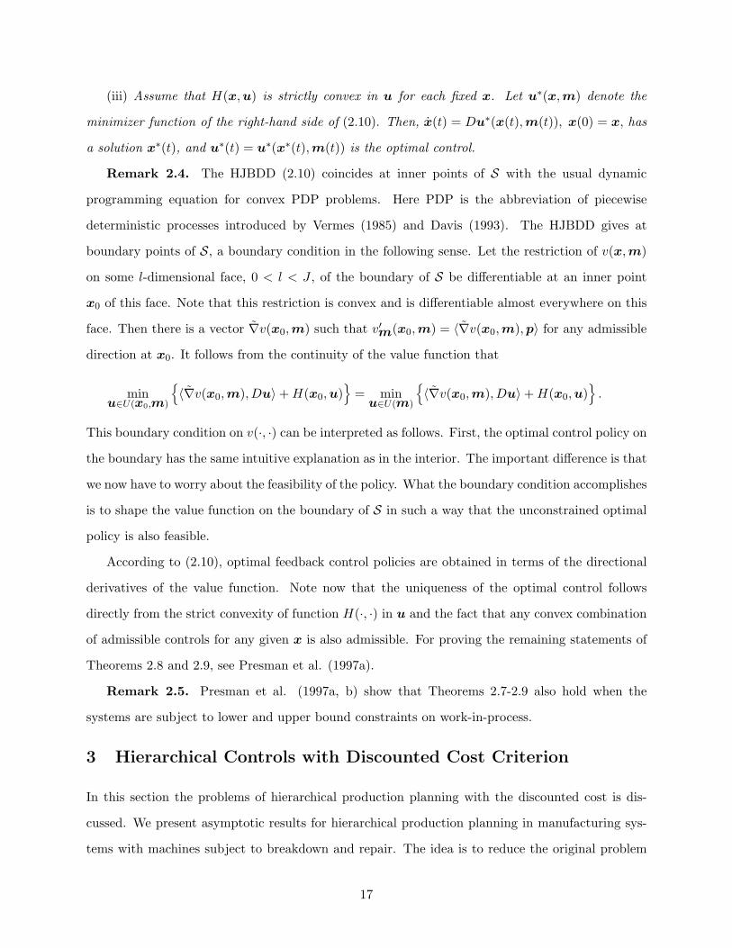
(iii) Assume that H(x,u) is strictly convex in u for each fixed x. Let u∗(x,m) denote the
minimizer function of the right-hand side of (2.10). Then, x(t) = Du∗(x(t),m(t)), x(0) = x, has
a solution x∗(t), and u∗(t) = u∗(x∗(t), m(t)) is the optimal control.
Remark 2.4. The HJBDD (2.10) coincides at inner points of S with the usual dynamic
programming equation for convex PDP problems. Here PDP is the abbreviation of piecewise
deterministic processes introduced by Vermes (1985) and Davis (1993). The HJBDD gives at
boundary points of S, a boundary condition in the following sense. Let the restriction of v(x, m)
on some l-dimensional face, 0 < l < J , of the boundary of S be differentiable at an inner point
x0 of this face. Note that this restriction is convex and is differentiable almost everywhere on this
face. Then there is a vector ∇v(x0, m) such that v′m(x0,m) = 〈∇v(x0, m), p〉 for any admissible
direction at x0. It follows from the continuity of the value function that
minu∈U(x0,m)
〈∇v(x0, m), Du〉+ H(x0, u)
= min
u∈U(m)
〈∇v(x0, m), Du〉+ H(x0, u)
.
This boundary condition on v(·, ·) can be interpreted as follows. First, the optimal control policy on
the boundary has the same intuitive explanation as in the interior. The important difference is that
we now have to worry about the feasibility of the policy. What the boundary condition accomplishes
is to shape the value function on the boundary of S in such a way that the unconstrained optimal
policy is also feasible.
According to (2.10), optimal feedback control policies are obtained in terms of the directional
derivatives of the value function. Note now that the uniqueness of the optimal control follows
directly from the strict convexity of function H(·, ·) in u and the fact that any convex combination
of admissible controls for any given x is also admissible. For proving the remaining statements of
Theorems 2.8 and 2.9, see Presman et al. (1997a).
Remark 2.5. Presman et al. (1997a, b) show that Theorems 2.7-2.9 also hold when the
systems are subject to lower and upper bound constraints on work-in-process.
3 Hierarchical Controls with Discounted Cost Criterion
In this section the problems of hierarchical production planning with the discounted cost is dis-
cussed. We present asymptotic results for hierarchical production planning in manufacturing sys-
tems with machines subject to breakdown and repair. The idea is to reduce the original problem
17
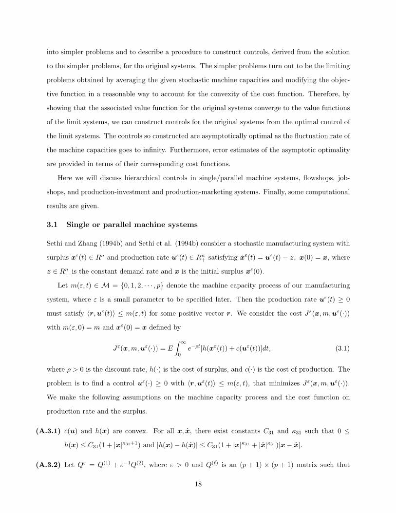
into simpler problems and to describe a procedure to construct controls, derived from the solution
to the simpler problems, for the original systems. The simpler problems turn out to be the limiting
problems obtained by averaging the given stochastic machine capacities and modifying the objec-
tive function in a reasonable way to account for the convexity of the cost function. Therefore, by
showing that the associated value function for the original systems converge to the value functions
of the limit systems, we can construct controls for the original systems from the optimal control of
the limit systems. The controls so constructed are asymptotically optimal as the fluctuation rate of
the machine capacities goes to infinity. Furthermore, error estimates of the asymptotic optimality
are provided in terms of their corresponding cost functions.
Here we will discuss hierarchical controls in single/parallel machine systems, flowshops, job-
shops, and production-investment and production-marketing systems. Finally, some computational
results are given.
3.1 Single or parallel machine systems
Sethi and Zhang (1994b) and Sethi et al. (1994b) consider a stochastic manufacturing system with
surplus xε(t) ∈ Rn and production rate uε(t) ∈ Rn+ satisfying xε(t) = uε(t)− z, x(0) = x, where
z ∈ Rn+ is the constant demand rate and x is the initial surplus xε(0).
Let m(ε, t) ∈ M = 0, 1, 2, · · · , p denote the machine capacity process of our manufacturing
system, where ε is a small parameter to be specified later. Then the production rate uε(t) ≥ 0
must satisfy 〈r, uε(t)〉 ≤ m(ε, t) for some positive vector r. We consider the cost Jε(x,m, uε(·))with m(ε, 0) = m and xε(0) = x defined by
Jε(x,m, uε(·)) = E
∫ ∞
0e−ρt[h(xε(t)) + c(uε(t))]dt, (3.1)
where ρ > 0 is the discount rate, h(·) is the cost of surplus, and c(·) is the cost of production. The
problem is to find a control uε(·) ≥ 0 with 〈r, uε(t)〉 ≤ m(ε, t), that minimizes Jε(x,m, uε(·)).We make the following assumptions on the machine capacity process and the cost function on
production rate and the surplus.
(A.3.1) c(u) and h(x) are convex. For all x, x, there exist constants C31 and κ31 such that 0 ≤h(x) ≤ C31(1 + |x|κ31+1) and |h(x)− h(x)| ≤ C31(1 + |x|κ31 + |x|κ31)|x− x|.
(A.3.2) Let Qε = Q(1) + ε−1Q(2), where ε > 0 and Q(`) is an (p + 1) × (p + 1) matrix such that
18
Q(`) = (q(`)ij ) with q
(`)ij ≥ 0 if i 6= j and q
(`)ii = −∑
j 6=i q(`)ij , for ` = 1, 2. The capacity process
0 ≤ m(ε, t) ∈M is a finite state Markov process governed by Q(ε), i.e., Lψ(·)(i) = Qεψ(·)(i),for any function ψ on M.
(A.3.3) The Q(2) is weakly irreducible, i.e., the equations νQ(2) = 0 and∑p
j=0 νj = 1 have a unique
solution ν = (ν0, ν1, · · · , νp) > 0. We call ν to be the equilibrium distribution of Q(2).
Remark 3.1. Jiang and Sethi (1991) and Khasminskii et al. (1997) consider a model in which
the irreducibility assumption in (A.3.4) can be relaxed to incorporate machine state processes with
a generator that consists of several irreducible submatrices. In these models, some jumps are
associated with a fast process, while others are associated with a slow process; see Section 5.4.
Definition 3.1. We say that a control uε(·) = uε(t) : t ≥ 0 is admissible if (i) uε(t) ≥ 0 is
a measurable process adapted to Ft = σm(ε, s), 0 ≤ s ≤ t ; (ii) 〈r, uε(t)〉 ≤ m(ε, t) for all t ≥ 0.
We use Aε(m) to denote the set of all admissible controls with the initial condition m(ε, 0) = k.
Then our control problem can be written as follows:
Pε :
minimize Jε(x,m, uε(·)) = E∫∞0 e−ρt[h(xε(t)) + c(uε(t))]dt,
subject to xε(t) = uε(t)− z,xε(0) = x, uε(·) ∈ Aε(m),
value function vε(x,m) = infuε(·)∈Aε(m) Jε(x,m, uε(·)).(3.2)
Similar to Theorem 2.1, one can show that the value function vε(x,m) is convex in x for each m.
The value function vε(·, ·) satisfies the dynamic programming equation
ρvε(x,m) = minu≥0,r·u≤m
[〈(u− z), ∂vε(x,m)/∂x〉+ h(x) + c(u)] + Lvε(x, ·)(m),m ∈M, (3.3)
in the sense of viscosity solutions. Sethi et al. (1994b) consider a control problem in which the
stochastic machine capacity process is averaged out. Let A0 denote the control space
A0 = U(t) = (u0(t), u1(t), · · · ,up(t)) : ui(t) ≥ 0, 〈r, ui(t)〉 ≤ i, 0 ≤ i ≤ p.
Then we define the control problem P0 as follows:
P0 :
minimize J0(x, U(·)) = E∫∞0 e−ρt[h(x(t)) +
∑pi=0 νic(ui(t))]dt,
subject to x(t) =∑p
i=0 νiui(t)− z, x(0) = x, U(·) ∈ A0,
value function v(x) = infU(·)∈A0 J0(x,u(·)).(3.4)
Sethi and Zhang (1994b) and Sethi et al. (1994b) construct a solution of Pε from a solution of P0,
and show it to be asymptotically optimal as stated below.
19
Theorem 3.1. (i) There exists a constant C32 such that |vε(x,m)− v(x)| ≤ C32(1+ |x|κ31)√
ε.
(ii) Let U(·) ∈ A0 denote an ε-optimal control. Then, uε(t) =∑p
i=0 Im(ε,t)=iui(t) is asymp-
totically optimal, i.e.,
|Jε(x,m, uε(·))− vε(x,m)| ≤ C32(1 + |x|κ31)√
ε. (3.5)
(iii) Assume in addition that c(u) is twice differentiable with (∂2c(u)∂ui∂uj
) ≥ c0In×n, the function
h(·) is differentiable, and constants C33 and κ32 > 0 exist such that
∣∣h(x + y)− h(x)− 〈h′x(x), y〉∣∣ ≤ C33(1 + |x|κ32)|y|2.
Then, there exists a locally Lipschitz optimal feedback control U∗(x) for P0. Let
u∗(x,m(ε, t))) =p∑
i=0
Im(ε,t)=iui∗(x). (3.6)
Then, uε(t) = u∗(x(t),m(ε, t)) is an asymptotically optimal feedback control for Pε with the con-
vergence rate of√
ε, i.e., (3.5) holds.
Insight 3.1. (Based on Theorem 3.1(i) and (ii).) If the capacity transition rate is sufficiently
fast in relation to the discount rate, then the value function is essentially independent of the initial
capacity state. This is because the transients die out and the capacity process settles into its
stationary distribution long before the discount factor e−ρt has decreased substantially from its
initial value of 1.
Remark 3.2. Part (ii) of the theorem states that from an ε-optimal open-loop control of the
limiting problem, we can construct an√
ε-optimal open-loop control for the original problem. With
further restrictions on the cost function, Part (iii) of the theorem states that from the ε-optimal
feedback control of the limiting problem, we can construct an√
ε-optimal feedback control for the
original problem.
Remark 3.3. It is important to point out that the hierarchical feedback control (3.6) can be
shown to be a threshold-type control if the production cost c(u) is linear. Of course, the value of
the threshold depends on the state of the machines. For single product problems with constant
demand, this means that production takes place at the maximum rate if the inventory is below
the threshold, no production takes place above it, and production rate equals the demand rate
once the threshold is attained. This is also the form of the optimal policy for these problems as
shown, e.g., in Kimemia and Gershwin (1983), Akella and Kumar (1986), and Sethi et al. (1992a).
20
The threshold level for any given machine capacity state in these cases is also known as a hedging
point in that state following Kimemia and Gershwin (1983). In these simple problems, asymptotic
optimality is maintained as long as the threshold, say, θ(ε), goes to 0 as ε → 0. Thus, there is a
possibility of obtaining better policies than (3.6) that are asymptotically optimal. In fact, one can
even minimize over the class of threshold policies for the parallel-machines problems discussed in
this section.
Soner (1993) and Sethi and Zhang (1994c) consider Pε in which Q = 1εQ(u) depends on the
control variable u. They show that under certain assumptions, the value function vε converges
to the value function of a limiting problem. Moreover, the limiting problem can be expressed in
the same form as P0 except that the equilibrium distribution νi, i = 0, 1, 2, · · · , p, are now control-
dependent. Thus, νi in Assumption (A.3.3) is now replaced by νi(u(t)) for each i; see also (3.22).
Then an asymptotically optimal control for Pε can be obtained as in (3.6) from the optimal control
of the limiting problem. As yet, no convergence rate has been obtained in this case.
An example of Q(u) in a one-machine case with two (up and down) states is
Q(u) =
−µ µ
λ(u) −λ(u)
.
Thus, the breakdown rate λ(u) of the machine depends on the rate of production u, while the
repair rate µ is independent of the production rate. These are reasonable assumptions in practice.
3.2 Dynamic flowshops
For manufacturing systems with N machines in tandem and with unlimited capacities of the internal
buffers, Sethi et al. (1992c) obtain a limiting problem. Then they use a near-optimal control of the
limiting problem to construct an open-loop control for the original problem, which is asymptotically
optimal as the transition rates between the machine states go to infinity. The case of a limited
capacity internal buffer is treated in Sethi et al. (1992d, 1993, 1997c). Recently, based on the
Lipschitz continuity of the value function given by Presman et al. (1997b), Sethi et al. (2000d)
construct a hierarchical control for the N -machine flowshop with limited buffers.
Since many of the flowshop results have been generalized to the more general case of jobshops
discussed in the next section, we shall not provide a separate review of the flowshop results. How-
ever, results derived specifically for flowshops will be given at the end of the next section as special
21
cases of the jobshop.
3.3 Dynamic jobshops
Sethi and Zhou (1994) consider hierarchical production planning in a general manufacturing system
given in Section 2.3. For the jobshop (∆, Π,K), let uεij(t) be the control at time t associated with
arc (i, j), (i, j) ∈ Π. Suppose we are given a stochastic process m(ε, t) = (m1(ε, t), ..., mN (ε, t)) on
the probability space (Ω,F , P ) with mn(ε, t) representing the capacity of the nth machine at time
t, n = 1, ..., N , where ε > 0 is a small parameter to be precisely specified later. The controls uεij(t)
with (i, j) ∈ Kn, n = 1, ..., N , t ≥ 0, should satisfy the following constraints:
0 ≤∑
(i,j)∈Kn
uεij(t) ≤ mn(ε, t) for all t ≥ 0, n = 1, ..., N, (3.7)
where we have assumed that the required machine capacity pij (for unit production rate of type j
from part type i) equals 1, for convenience in exposition. The analysis in this paper can be readily
extended to the case when the required machine capacity for the unit production rate of part j
from part i is any given positive constant.
We denote the level at time t in buffer i by xεi (t), i ∈ ∆ \ 0, Nb + 1. Note that if xε
i (t) > 0,
i = 1, ..., Nb, we have an inventory in buffer i, and if xεi (t) < 0, i = d+1, ..., Nb, we have a shortage
of finished product i. The dynamics of the system are, therefore,
xεi (t) =
(∑i−1`=0 uε
`i(t)−∑Nb
`=i+1 uεi`(t)
), 1 ≤ i ≤ d,
xεi (t) =
(∑d`=0 uε
`i(t)− zi
), d + 1 ≤ i ≤ Nb,
(3.8)
with xε(0) := (xε1(0), ..., xε
Nb(0)) = (x1, ..., xNb
) = x. Let uε`(t) = (uε
`,`+1(t), ..., uε`,Nb
(t))′, ` =
0, ..., d, and uεd+1(t) = (zd+1, ..., zNb
)′. Similar to Section 2.3, we rewrite (3.8) in the vector form as
xε(t) = (xε1(t), ..., x
εNb
(t))′ = Duε(t).
Definition 3.2. We say that a control uε(·) ∈ U is admissible with respect to the initial state
vector x = (x1, · · · , xNb) ∈ S and m ∈ M, if (i) uε(·) is an Fε
t -adapted measurable process with
Fεt = σm(ε, s) : 0 ≤ s ≤ t; (ii) uε(t) ∈ U(m(ε, t)) for all t ≥ 0; and (iii) the corresponding state
process xε(t) = (xε1(t), · · · , xε
Nb(t)) ∈ S for all t ≥ 0.
Let Aε(x, m) denote the set of all admissible control with respect to x ∈ S and the machine
capacity vector m. The problem is to find an admissible control uε(·) that minimize the cost
22
criterion
Jε(x, m, uε(·)) = E
∫ ∞
0e−ρt[h(xε(t)) + c(uε(t))]dt, (3.9)
where h(·) defines the surplus cost, c(·) is the production cost, x is the initial state, and m is the
initial value of m(ε, t). The value function is then defined as
vε(x, m) = infuε(·)∈Aε(x,m)
Jε(x, m,uε(·)). (3.10)
We impose the following assumptions on the capacity process m(ε, t) = (m1(ε, t), ..., mN (ε, t))
and the cost functions h(·) and c(·) throughout this section.
(A.3.4) Let M = m1, ...,mp for some given integer p ≥ 1, where mj = (mj1, ...,m
jN ), with mj
k, k =
1, ..., N , denoting the capacity of the kth machine, j = 1, ..., p. The capacity process mε(t) ∈M is a finite state Markov chain with the infinitesimal generator Q = Q(1) + ε−1Q(2), where
Q(1) = (q(1)ij ) and Q(2) = (q(2)
ij ) are matrices such that q(`)ij ≥ 0 if j 6= i, and q
(`)ii = −∑
j 6=i q(`)ij
for ` = 1, 2. Moreover, Q(2) is irreducible and, without any loss of generality, it is taken to be
the one that satisfies minij|q(2)ij | : q
(2)ij 6= 0 = 1.
(A.3.5) Assume that Q(2) is weakly irreducible. Let ν = (ν1, ..., νp) denote the equilibrium distribution
of Q(2), that is, ν is the only nonnegative solution to the equations νQ(2) = 0 and∑p
i=1 νi = 1.
(A.3.6) h(·) and c(·) are convex functions. For all x, x ∈ S and u, u, there exist constants C34 and
κ32 ≥ 0 such that 0 ≤ h(x) ≤ C34(1 + |x|κ32), |h(x)− h(x)| ≤ C34(1 + |x|κ32 + |x|κ32)|x− x|,and |c(u)− c(u)| ≤ C34|u− u|.
We use Pε to denote our control problem:
Pε :
min Jε(x, m,uε(·)) = E∫∞0 e−ρt[h(xε(t)) + cuε(t))]dt,
s.t. xε(t) = Duε(t), xε(0) = x, uε(·) ∈ Aε(x,m),
value fn vε(x, m) = infuε(·)∈Aε(x,m) Jε(x, m, uε(·)).(3.11)
In order to obtain the limiting problem, we consider the deterministic controls defined below.
Definition 3.3. For x ∈ S, let A0(x) denote the set of the following measurable controls
U(·) = ((u1,00 (·), ...,u1,0
d+1(·)), ..., (up,00 (·), ...,up,0
d+1(·))) with∑
(i,j)∈Knu`,0
ij (t) ≤ m`n, ` = 1, ..., p, n =
1, ..., N , and the corresponding solution x(·) of the system
xj(t) =∑j−1
`=0
∑pi=1 νiu
i,0`j (t)−∑Nb
`=j+1
∑pi=1 νiu
i,0j` (t), xj(0) = xj , 1 ≤ j ≤ d,
xj(t) =∑d
`=0
∑pi=1 νiu
i,0`j (t)− zj , xj(0) = xj , d + 1 ≤ j ≤ Nb,
(3.12)
23
satisfies x(t) ∈ S for all t ≥ 0.
The objective of the limiting problem is to choose a control U(·) ∈ A0 that minimizes
J0(x, U(·)) =∫ ∞
0e−ρt
[h(x(t)) +
p∑
`=1
ν`c(u`,0(t))
]dt.
We write (3.12) in the vector form x(t) = D∑p
`=1 ν`u`,0(t), x(0) = x. We use P0 to denote the
limiting problem and derive it as follows:
P0 :
min J0(x, U(·)) =∫∞0 e−ρt[h(x(t)) +
∑p`=1 ν`c(u`,0(t))]dt,
s.t. x(t) = D∑p
`=1 ν`u`,0(t), x(0) = x, U(·) ∈ A0(x),
value fn. v(x) = infU(·)∈A0(x) J0(x, U(·)).
Based on the Lipschitz continuity of the value function given in Section 2.3, Sethi and Zhou
(1994) prove the following theorem which says that the problem P0 is indeed a limiting problem
in the sense that the value function vε(x,m) of Pε converges to the value function v(x) of P0.
Furthermore, the theorem also gives the corresponding convergence rate.
Theorem 3.2. For each δ ∈ (0, 12), there exists a positive constant C35 such that for all x ∈ S
and sufficiently small ε, we have |vε(x, m)− v(x)| ≤ C35(1 + |x|κ32)ε12−δ.
Insight 3.2. Comparison of Theorems 3.1 and 3.2 reveals that there is a slight loss in the
order of the error bound when going from a single/parallel machine system to a jobshop on account
of the state constraints inherent in a jobshop. The presence of the state constraints results in a
capacity loss phenomenon, because a machine, even while in the working order, cannot produce if
the output buffer provides an input to a failed machine.
Sethi et al. (2002) also show that Theorem 3.2 is true for a general jobshop system with limited
buffers. Similar to Theorem 3.1, for a given x ∈ S, they describe the procedure of constructing
an asymptotic optimal control uε(·) ∈ Aε(x, m) of the original problem Pε beginning with any
near-optimal control U(·) ∈ A0(x) of the limiting problem P0. We illustrate their procedure for the
special case of a flowshop with two-machine and single product, that is, (3.8) with m = 1, Nb = 2
and uε02(t) ≡ 0. First we focus on the open-loop control. Let us fix an initial state x ∈ S. Let
U(·) = (u1,0(·), · · · , up,0(·)) ∈ A0, where uj,0(t) = (uj,001 (t), uj,0
12 (t)) is an ε12−δ-optimal control for P0,
i.e., |J0(x, U(·))− v(x)| ≤ ε12−δ. Because the work-in-process level must be nonnegative, unlike in
the case of parallel machine systems, the control∑p
j=1 Im(ε,t)=mjuj,0(t) may not be admissible.
Thus, we need to modify it. Let us define a time t∗ ≤ ∞ as follows: t∗ = inft :∫ t0 [
∑pj=1(m
j1 −
24
νjuj,001 (s) + νju
j,012 (s))]ds ≥ ε
12−δ. We define another control process U(t) = (u1,0(·), · · · , up,0(·)) as
follows: for j = 1, · · · , p,
uj,0(t) = (uj,001 (t), uj,0
12 (t)) =
(mj1, 0) if t < t∗,
(uj,001 (t), uj,0
12 (t)) if t ≥ t∗.(3.13)
It is easy to check that U(·) ∈ A0(x). Let
wε(t) =p∑
j=1
νjuj(t)Im(ε,t)=mj, (3.14)
and let yε(t) = (yε1(t), y
ε2(t)) be the corresponding trajectory defined as
yε1(t) = x1 +
∫ t0(wε
1(s)− wε2(s))ds,
yε2(t) = x2 +
∫ t0(wε
2(s)− z2)ds.
Note that E|yε(t) − x(t)|2 ≤ C(1 + t2)ε. However, yε(t) may not be in S for some t ≥ 0.
To obtain an admissible control for Pε, we need to modify yε(t) so that the state trajectory
stays in S. This is done as follows. Let uε(t) = (uε1(t), u
ε2(t)) := yε(t)Iyε
1(t)≥0. Then, for the
control uε(·) ∈ Aε(x,m) constructed (3.13)-(3.14) above, it is shown in Sethi et al. (1993) that
|Jε(x, m, uε(·))− vε(x,m)| = O(ε12−δ). Moreover, the case of more than two machines is treated
in Sethi et al. (1992c).
Next, we give explicitly an asymptotically optimal feedback control for a two-machine flowshop.
The problem is addressed by Sethi and Zhou (1996a, b), who consider Pε in (3.11) with
c(u) = 0 and h(x) = c1x1 + c+2 x+
2 + c−2 x−2 , (3.15)
where c1, c+2 and c−2 are given nonnegative cost coefficients and x+
2 = maxx2, 0 and x−2 =
−minx2, 0. In order to illustrate their results, we choose a simple situation in which each of
the two machines has a capacity m when up and 0 when down, and has a breakdown rate λ > 0
and the repair rate µ > 0. Furthermore, we shall assume that the average capacity m = mµ/(λ + µ)
of each machine is strictly larger than the demand z2.
The optimal control of the corresponding limiting (deterministic) problem P0 is:
u(x) =
(0, 0) if x1 ≥ 0, x2 > 0,
(0, z2) if x1 > 0, x2 = 0,
(0, m) if x1 > 0, x2 < 0,
(m, m) if x1 = 0, x2 < 0,
(z2, z2) if x1 = 0, x2 = 0.
(3.16)
25
Insight 3.3. An optimal control is to get to (0, 0) in the cheapest possible way, and then stay
there.
From (3.16), Sethi and Zhou (1996a, b) construct the following asymptotically optimal feedback
control:
uε(x, m) =
(0, 0), x1 ≥ 0, x2 > θ2(ε),
(0,mink2, z2), x1 > θ1(ε), x2 = θ2(ε),
(0, k2), x1 > θ1(ε), x2 < θ2(ε),
(mink1, k2, k2), x1 = θ1(ε), x2 < θ2(ε),
(mink1, k2, z2, mink2, z2), x1 = θ1(ε), x2 = θ2(ε),
(k1, k2), 0 < x1 < θ1(ε), x2 < θ2(ε),
(k1, mink2, z2), 0 < x1 < θ1(ε), x2 = θ2(ε),
(k1, mink1, k2, z2), x1 = 0, x2 = θ2(ε),
(k1, mink1, k2), x1 = 0, x2 < θ2(ε),
(3.17)
where m = (k1, k2) with k1 ∈ 0,m and k2 ∈ 0,m, and (θ1(ε), θ2(ε)) → (0, 0) as ε → 0; see
Figure 1.
Note that the optimal control (3.16) of P0 uses the obvious bang-bang and singular controls to
go to (0, 0) and then stay there. In the same spirit, the control in (3.17) uses bang-bang and singular
controls to approach (θ1(ε), θ2(ε)). For a detailed heuristic explanation of asymptotic optimality,
see Samaratunga et al. (1997) and Sethi (1997); for a rigorous proof, see Sethi and Zhou (1996a,
b).
Remark 3.5. The policy in Figure 1 cannot be termed a threshold-type policy, since there
is no maximum tendency to go to x1 = θ1(ε), when the inventory level x1(t) is below θ1(ε) and
x2(t) > θ2(ε). In fact, Sethi and Zhou (1996a, b) show that a threshold-type policy, known also
as a Kanban policy, is not even asymptotically optimal when c1 > c+2 . Also, it is known that the
optimal feedback policy for two-machine flowshops involve switching manifolds that are much more
complicated than the manifolds x1 = θ1 and x2 = θ2 required to specify a threshold-type policy.
This implies that in the discounted flowshop problems, one cannot find an optimal feedback policy
within the class of threshold-type policies. While θ1 and θ2 could still be called hedging points,
there is no notion of optimal hedging points insofar as they are used to specify a feedback policy.
See Samaratunga et al. (1997) for a further discussion on this point.
26
3.4 Computational results
Connolly et al. (1992), Van Ryzin et al. (1993), Violette (1993), and Violette and Gershwin (1991)
have carried out a good deal of computational work in connection with manufacturing systems
without state constraints. Such systems include single or parallel machine systems described in
Sections 3.1, 3.2, and 3.3 as well as no-wait flowshops (or flowshops without internal buffers)
treated in Kimemia and Gershwin (1983). Darakananda (1989) developed a simulation software
called Hiercsim based on the control algorithms of Gershwin et al. (1985) and Gershwin (1989).
It should be noted that controls constructed in these algorithms have been shown under some
conditions to be asymptotically optimal by Sethi and Zhang (1994b) and Sethi et al. (1994b).
One of the main weaknesses of the early version of Hiercsim for the purpose of this review is
its inability to deal with internal storage, see also Violette and Gershwin (1991). Bai (1991) and
Bai and Gershwin (1990) developed a hierarchical scheme based on partitioning machines in the
original flowshop or jobshop into a number of virtual machines each devoted to single part type
production. Violette (1993) developed a modified version of Hiercsim to incorporate the method of
Bai and Gershwin (1990). Violette and Gershwin (1991) perform a simulation study indicating that
the modified method is efficient and effective. We shall not review it further, since the procedure
based on partitioning of machines is unlikely to be asymptotically optimal.
Sethi and Zhou (1996b) have constructed asymptotically optimal hierarchical controls uε(x, m),
given in (3.17) with switching manifolds depicted in Figure 1, for the two-machine flowshop defined
by (3.8) with d = 1, Nb = 1, and uε02(t) ≡ 0, and (3.15). Samaratunga et al. (1997) have compared
the performance of these hierarchical controls (HC) to that of optimal control (OC) and of two other
existing heuristic methods known as Kanban Control (KC) and Two-Boundary Control (TBC). Like
HC, KC is a two parameter policy defined as follows:
uεKC(x, m) =
(m1, 0) if 0 ≤ x1 < θ1(ε), x2 > θ2(ε),
uε(x,m) otherwise.(3.18)
Note that KC is a threshold-type policy. TBC is a three-parameter policy developed by Lou
and Van Ryzin (1989). Because it is much more complicated than HC or KC and because its
performance is not significantly different from HC as can be seen in Samaratunga et al. (1997),
we shall not discuss it any further in this survey. In what follows, we provide the computational
results obtained in Samaratunga et al. (1997) for the problem (3.11) and (3.15) with λ = 1, µ =
27
5,m = 2, c+1 = 0.1, c+
2 = 0.2, and c−2 = 1.0. Then we discuss the results.
In Table 1, different initial states are selected and the best parameter values are computed for
these different initial states for HC and KC; note from Remark 3.6 that in general there are no
parameter values that are best for all possible initial states. In the last row, the initial state (2.70,
1.59) is such that the best hedging point for HC and KC are (2.70,1.59). Table 2 uses the parameter
values obtained in Table 1 in the row with the initial state (0,0). Samaratunga et al. (1997) analyze
these computational results and provide the following comparison of OC and KC.
HC vs. OC: In Tables 1 and 2, the cost of HC is quite close to the optimal cost, if the initial state
is sufficiently removed from point (0,0). Moreover, the further the initial (x1, x2) is from point
(0,0), the better the approximation HC provides to OC. This is because the hedging points are
close to point (0,0), and hierarchical and optimal controls agree at points in the state space that
are further from (0,0) or further from hedging points. In these cases, transients contribute a great
deal to the total cost and transients of HC and OC agree in regions far away from (0,0).
HC vs. KC: Let us now compare HC and KC in detail. Of course, if the initial state is in a
shortage situation (x2 ≤ 0), then HC and KC must have identical costs. This can be easily seen in
Table 1 or Table 2 when initial (x1, x2) = (0, -5), (0, -10), (0, -20), (5, -5), (10, -10) and (20, -20).
On the other hand, if the initial surplus is positive, cost of HC is either the same as or slightly
smaller than the cost of KC, as should be expected. This is because, KC being a threshold-type
policy, the system approaches θ1(ε) even when there is large positive surplus, implying higher
inventory costs. In Tables 1 and 2, we can see this in rows with initial (x1, x2) = (0, 5), (0, 10),
(0, 20), and (20, 20). Moreover, by the same argument, the values of θ1(ε) for KC must not be
larger than those for HC in Table 1. Indeed, in cases with large positive surplus, the value of θ1(ε)
for KC must be smaller than that for HC. Furthermore, in these cases with positive surplus, the
cost differences in Table 2 must be larger than those in Table 1, since Table 2 uses hedging point
parameters that are best for initial (x1, x2) = (0,0). These parameters are the same for HC and
KC. Thus, the system with an initial surplus has higher inventories in the internal buffer with KC
than with HC.
Note also that if the surplus is very large, then KC in order to achieve lower inventory costs
sets θ1(ε) = 0, with the consequence that its cost is the same as that for HC. For example, this
happens when the initial (x1, x2) = (0,50) in Table 1. As should be expected, the difference in cost
28
for initial (x1, x2) = (0,50) in Table 2 is quite large compared to the corresponding difference in
Table 1.
3.5 Production-investment models
Sethi et al. (1992b) incorporate an additional capacity expansion decision in the model discussed
in Section 3.1. They consider a stochastic manufacturing system with the surplus xε(t) ∈ Rn and
production rate uε(t) ∈ Rn that satisfy xε(t) = uε(t) − z, xε(0) = x, where z ∈ Rn denotes the
constant demand rate and x is the initial surplus level. They assume uε(t) ≥ 0 and 〈r, uε(t)〉 ≤m(ε, t) for some r ≥ 0, where m(ε, t) is the machine capacity process described by (3.20). The
specification of m(ε, t) involves the instantaneous purchase of some given additional capacity at
some time τ , 0 ≤ τ ≤ ∞, at a cost of K, where τ = ∞ means not to purchase it at all; see Sethi et
al. (1994a) for an alternate model in which the investment in the additional capacity is continuous.
For the model under consideration, the control variable is a pair (τ, u(·)) of a Markov time τ ≥ 0
and a production process u(·) over time. The cost criterion Jε is given by
Jε(x,m, τ,uε(·)) = E
[∫ ∞
0e−ρtH(xε(t),uε(t))dt + Ke−ρτ
], (3.19)
where m(ε, 0) = m is the initial capacity and ρ > 0 is the discount rate. The problem is to find an
admissible control (τ, uε(·)) that minimizes Jε(x,m, τ,uε(·)).Define m1(ε, ·) and m2(ε, ·) as two Markov processes with state spaces M1 = 0, 1, · · · , p1
and M2 = 0, 1, · · · , p1 + p2, respectively. Here, m1(ε, ·) ≥ 0 denotes the existing production
capacity process and m2(ε, ·) ≥ 0 denotes the capacity process of the system if it were to be
supplemented by the additional new capacity at time 0. Let F1(t) = σm1(ε, s) : 0 ≤ s ≤ t and
F(t) = σm(ε, t) : 0 ≤ s ≤ t.Define the capacity process m(ε, t) as follows: For each F1(t)-Markov time τ ≥ 0,
m(ε, t) =
m1(ε, t) if t < τ,
m2(ε, t− τ) if t ≥ τ,and m(ε, τ) = m2(ε, 0) := m1(ε, τ) + p2. (3.20)
Here p2 denotes the maximum additional capacity resulting from the investment in the new capacity.
We make the following assumptions on the cost function H(·, ·) and the process m(ε, t).
(A.3.7) G(x, u) is a nonnegative jointly convex function that is strictly convex in either x or u
or both. For all x, x ∈ Rn and u, u ∈ Rn+, there exist constant C35 and κ33 such that
|H(x,u)−H(x, u)| ≤ C35[(1 + |x|κ33 + |x|κ33)|x− x|+ |u− u|].
29
(A.3.8) m1(ε, t) ∈ M1 and m2(ε, t) ∈ M2 are Markov processes with generators ε−1Q1 and ε−1Q2,
respectively, where Q1 = (q(1)ij ) and Q2 = (q(2)
ij ) are matrices such that q(`)ij ≥ 0 if i 6= j and
q(`)ii = −∑
i6=j q(`)ij for ` = 1, 2. Moreover, Q1 and Q2 are both irreducible.
Definition 3.4. We say that a control (τ, uε(·)) is admissible if (i) τ is an F1(t)-Markov time;
(ii) uε(t) is F(t)-adapted and 〈r, uε(t)〉 ≤ m(ε, t) for t ≥ 0.
We use Aε(x,m) to denote the set of all admissible controls (τ, uε(·)). Then the problem is:
Pε :
min(τ,uε(·))∈Aε Jε(x,m, τ,uε(·)),subject to xε(t) = uε(t)− z, xε(0) = x.
We use vε(x,m) to denote the value function of the problem and define an auxiliary value function
vεa(x, m) to be K plus the optimal cost with the capacity process m2(ε, t) with the initial capacity
m ∈ M2 and no future capital expansion possibilities. Then the dynamic programming equations
are as follows:
min minu≥0,〈r,u〉≤m
[〈(u− z), ∂vε(x,m)/∂x〉+ G(x, u)] + ε−1Q1vε(x, ·)(m)
−ρvε(x,m), vεa(x,m + p2)− vε(x,m) = 0, m ∈M1,
minu≥0,〈r,u〉≤m
[〈(u− z), ∂vεa(x, m)/∂x〉+ G(x, u)] + ε−1Q2v
εa(x, ·)(m)
−ρ(vεa(x,m)−K) = 0, m ∈M2.
Let ν(1) = (ν(1)0 , ν
(1)1 , · · · , ν(1)
p1 ) and ν(2) = (ν(2)0 , ν
(2)1 , · · · , ν(2)
p1+p2) denote the equilibrium distributions
of Q1 and Q2, respectively. We now proceed to develop the limiting problem. We first define
the control sets for the limiting problem. Let U1 = (u0, · · · , up1) : ui ≥ 0, 〈r, ui〉 ≤ i and
U2 = (u0, · · · , up1+p2) : ui ≥ 0, 〈r, ui〉 ≤ i. Then U1 ⊂ Rn×(p1+1) and U2 ⊂ Rn×(p1+p2+1).
Definition 3.5. We use A0(x) to denote the set of the following controls (admissible controls
for the limiting problem): (i) A deterministic time σ; (ii) A deterministic U(t) such that for t < σ,
U(t) = (u0(t), · · · ,up1(t)) ∈ U1 and for t ≥ σ, U(t) = (u0(t), · · · ,up1+p2(t)) ∈ U2.
Let
J0(x, σ, U(·)) =∫ σ
0e−ρt
p1∑
i=0
ν(1)i G(x(t), ui(t))dt
+∫ ∞
σe−ρt
p1+p2∑
i=0
u(2)i G(x(t),ui(t))dt + e−ρσK,
30
u(t) =
∑p1i=0 ν
(1)i ui(t) if t < σ,
∑p1+p2i=0 νiu
i(t) if t ≥ σ.
We can now define the following limiting optimal control problem:
P0 :
min(σ,U(·))∈A0
J0(x, σ, U(·))
subject to x(t) = u(t)− z, x(0) = x.
(3.21)
Let v(x) denote the value functions for P0, and va(x)) denote min(0,U(·))∈A0 J0(x, 0, U(·)). Let
(τ, U(·)) ∈ A0 denote any admissible control for the limiting problem P0, where
U(t) =
(u0(t), · · · , up1(t)) ∈ U1 if t < σ,
(u0(t), · · · , up1+p2(t)) ∈ U2 if t ≥ σ.
We take
uε(t) =
∑p1i=0 ui(t)Im1(ε,t)=i if t < τ,
∑p1+p2i=0 ui(t)Im2(ε,t)=i if t ≥ τ.
Then the control (τ, uε(·)) is admissible for Pε. The following result is proved in Sethi et al.
(1992b).
Theorem 3.3. (i) There exists a constant C36 such that |vε(x,m)−v(x)|+ |vεa(x, m)−va(x)| ≤
C36(1 + |x|κ33)√
ε.
(ii) Let (τ, U(·)) ∈ A0 be an ε-optimal control for the limiting problem P0 and let (τ, uε(·)) ∈ Aε
be the control constructed above. Then, (τ, uε(·)) is asymptotically optimal with error bound√
ε,
i.e., |Jε(x,m, τ,uε(·))− vε(x,m)| ≤ C36(1 + |x|κ33)√
ε.
3.6 Other multilevel models
Sethi and Zhang (1992b, 1995a) extend the model in Section 3.1 to incorporate promotional or
advertising decisions that influence the product demands. Zhou and Sethi (1994) demonstrate how
workforce and production decisions can be decomposed hierarchically in a stochastic version of
the classical HMMS model (see Holt et al. (1960)). Manufacturing systems involving preventive
maintenance are studied by Boukas and Haurie (1990), Boukas (1991), Boukas et al. (1993), and
Boukas et al. (1994). The maintenance activity involves lubrication, routine adjustments, etc.,
which reduce the machine failure rates. The objective in these systems is to choose the rate of
31
maintenance and the rate of production in order to minimize the total discounted cost of surplus,
production, and maintenance.
In this section, we shall only discuss the model developed in Sethi and Zhang (1995a), who
consider the case when both capacity and demand are finite state Markov processes constructed
from generators that depend on the production and promotional decisions, respectively. In order
to specify their marketing-production problem, let m(ε, t) ∈ M as in Section 3.1 and z(δ, t) ∈z0,z1, · · · ,zp for a given δ, denote the capacity process and the demand process, respectively.
Definition 3.6. We say that a control (uε(·), w(·)) = (uε(t), wδ(t)) : t ≥ 0 is admis-
sible, if (i) (uε(·), wδ(·)) is right-continuous having left-hand limit (RCLL); (ii) (uε(·), wδ(·)) is
σ(m(ε, s), z(δ, s)) : 0 ≤ s ≤ t-adapted, and satisfies uε(t) ≥ 0, 〈r,uε(t)〉 ≤ m(ε, t), and
0 ≤ wδ(t) ≤ 1 for all t ≥ 0.
We use Aε,δ(x,m, z) to denote the set of all admissible controls. Then the control problem can
be written as follows:
Pε,δ :
maximize Jε,δ(x,m, z, uε(·), wδ(·))= E
∫∞0 e−ρtG(xε,δ(t), z(δ, t),uε(t), wδ(t))dt
subject to
xε,δ(t) = uε(t)− z(δ, t), xε,δ(0) = x
m(ε, t) ∼ ε−1Q(uε(t)), m(ε, 0) = m
z(δ, t) ∼ δ−1Q(w(t)), z(δ, 0) = z
(u(·), wδ(·)) ∈ Aε,δ(x.m,z).
value function vε,δ(x,m, z) = inf(uε(·),wδ(·))∈Aε,δ(x,m,z)
Jε,δ(x, m,z,uε(·), wδ(·))
(3.22)
where by m(ε, t) ∼ ε−1Q(uε(t)), we mean that the Markov process m(ε, t) has the generator
ε−1Q(uε(t)). We use A0,δ to denote the admissible control space
A0,δ = (U(t), w(t)) = (u0(t), u1(t), · · · ,up(t), w(t)) : ui(t) ≥ 0, 〈r,ui(t)〉 ≤ i, 0 ≤ w(t) ≤ 1,
(U(t), w(t)) is σz(δ, s) : 0 ≤ s ≤ t adapted and RCLL,
32
for the problem
P0,δ :
maximize J0,δ(x, z, U(·), w(·))
=∫ ∞
0e−ρt
p∑
i=0
νi(U(t))G(xδ(t), z(δ, t), ui(t), w(t))dt
subject to
xδ(t) =p∑
i=0
νi(U(t))ui(t)− z(δ, t), xδ(0) = x
z(δ, t) ∼ 1δQ(w(t)), z(δ, 0) = z
(U(·), w(·)) ∈ A0,δ.
value function v0,δ(x, z) = inf(U(·),w(·))∈A0,δ
J0,δ(x, z, U(·), w(·)).
(3.23)
Let (U(·), w(·)) ∈ A0,δ denote an optimal open-loop control. We construct uε,δ(t) =∑p
i=0 ui(t)Im(ε,t)=i
and wε,δ(t) = w(t). Then (uε,δ(t), wε,δ(t)) ∈ Aε,δ, and it is asymptotically optimal, i.e.,
limδ→0
|Jε,δ(x,m, z, uε,δ(·), wε,δ(·))− vε,δ(x,m, z)| = 0.
Similarly, let (U(x, z), w(x, z)) ∈ Aε,δ denote an optimal feedback control for P0,δ. Suppose that
(U(x,z), w(x, z)) is locally Lipschitz for each z. Let uε,δ(t) =∑p
i=0 ui(xε,δ(t),m(ε, t), z(δ, t))Im(ε,t)=i
and wε,δ(t) = w(xε,δ(t), z(δ, t)). Then the feedback control (uε,δ(·), wε,δ(·)) is asymptotically opti-
mal for Pε,δ, i.e.,
limδ→0
|Jε,δ(x,m, z, uε,δ(·), wε,δ(·))− vε,δ(x,m, z)| = 0.
We have described only the hierarchy that arises from a large δ and a small ε. In this case,
promotional decisions are obtained under the assumption that the available production capacity is
equal to the average capacity. Subsequently, production decisions taking into account the stochastic
nature of the capacity can be constructed. Other possible hierarchies result when both δ and ε are
small or when ε is large and δ is small.
3.7 Single or parallel machine systems with risk-sensitive discounted cost cri-terion
Consider the single/parallel machine system producing multiple products described in Subsection
3.1, but with the risk-sensitive discounted cost criterion defined by
Jε,√
ε(uε(·)) =√
ε log E
[exp
1√ε
∫ ∞
0e−ρt[h(xε(t)) + c(uε(t))]dt
]. (3.24)
A motivation for choosing this risk-sensitive criterion is to incorporate the decision maker’s attitude
toward risk. In (3.24),√
ε is called the risk-sensitivity coefficient. A positive coefficient indicates a
33
risk-averse behavior, whereas√
ε = 0 signifies risk neutrality. The problem is then as follows:
Pε,√
ε :
minimize Jε,√
ε(uε(·)),subject to xε(t) = uε(t)− z, xε(0) = x, uε(·) ∈ Aε(m),
value function vε,√
ε(x,m) = infuε(·)∈Aε(m)
Jε,√
ε(uε(·)).
For this problem, Zhang (1995) establishes results similar to Theorem 3.1.
In the next two sections we focus on the long-run average cost criterion, which presents a stark
contrast to the discounted-cost criterion. The discounted-cost criterion considers near-term costs
to be more important than costs occurring in the long term. The long-run cost criterion, on the
other hand, ignores the near-term costs and considers only the distant future costs. In Section
4, we consider the theory of optimal control of stochastic manufacturing problems with the long-
run average cost criterion. We use the vanishing discount approach for this purpose. Section 5 is
concerned with hierarchical controls for long-run average cost problems, for risk-sensitive average
cost problems, and for Markov decision processes with weak and strong interactions.
4 Optimal Control with Long-Run Average Cost Criteria
Beginning with Bielecki and Kumar (1988), there has been a considerable interest in studying the
problem of convex production planning in stochastic manufacturing systems with the objective of
minimizing long-run average cost. Bielecki and Kumar (1988) dealt with a single machine (with
two states: up and down), single product problem with linear holding and backlog costs. Because
of the simple structure of their problem, they were able to obtain an explicit solution, and thus
verify the optimality of the resulting policy. They showed that the so-called hedging point policy is
optimal in their simple model. It is a policy to produce at full capacity if the surplus is smaller than
a threshold level, produce nothing if the surplus is higher than the threshold level, and produce as
much as possible, but no more than the demand rate when the surplus is at the threshold level.
Sharifnia (1988) dealt with an extension of the Bielecki-Kumar model with more than two
machine states. Liberopoulous and Caramanis (1995) showed that Sharifnia’s method for evaluating
hedging point policies applies even when the transition rates of the machine states depend on
the production rate. Liberopoulous and Hu (1995) obtained monotonicity of the threshold levels
corresponding to different machine states. Srivatsan and Dallery (1998) generalized the Bielecki-
Kumar problem to allow for two products. They limited their focus to only the class of hedging
34
point policies and attempted to partially characterize an optimal solution within that class. Bai
and Gershwin (1990) and Bai (1991) use heuristic argument to obtain suboptimal controls in two-
machine flowshops. In addition to nonnegative constraints on the inventory levels in the internal
buffer, they also consider inventory level in this buffer to be bounded above by the size of the buffer.
Moreover, Srivatsan et al. (1994) apply their results to semiconductor manufacturing (jobshop). All
of these papers, however, are heuristic in nature, since they do not rigorously prove the optimality
of the policies for their extensions of the Bielecki-Kumar model.
Presman et al. (1998) extend the hedging point policy to the problem of two products by using
the potential function related to the dynamic programming equation of the two-product problem.
Using a verification theorem for the two-product problem, they prove the optimality of the hedging
point policy. Furthermore, Sethi and Zhang (1999) prove the optimality of the hedging point policy
for a general n-product problem under a special class of cost functions. For its deterministic version,
Sethi et al. (1996) provide explicit optimal control policies and the value function.
The difficulty in proving the optimality in general rather than for these special cases lies in the
fact that when the problem is generalized to include convex cost and multiple machine capacity
levels, explicit solutions are no longer possible. One then needs to develop appropriate dynamic
programming equations, existence of their solutions, and verification theorems for optimality. In
this section, we will review some works related to this.
4.1 Single or parallel machine systems
We consider an n-product manufacturing system given in Section 2.1. For any u(·) ∈ A(m), define
J(x,m, u(·)) = lim supT→∞
1T
E
∫ T
0[h(x(t)) + c(u(t))]dt, (4.1)
where x(·) is the surplus process corresponding to the production process u(·) with x(0) = x,
and h(·), c(·) and m(·) are as given in Section 2.1. Our goal is to choose u(·) ∈ A(m) so as to
minimize the average cost J(x,m, u(·)). In addition to Assumption (A.2.2) on the production cost
c(·), we assume the production capacity process m(·) and the surplus cost function h(·) to satisfy
the following:
(A.4.1) h(·) is nonnegative and convex with h(0) = 0. There are positive constants C41, C42, and
κ41 such that h(x) ≥ C41|x|κ41 − C42. Moreover, there are constants C43 and κ42 such that
|h(x)− h(x)| ≤ C43(1 + |x|k42−1 + |x)|κ42−1)|x− x|.
35
(A.4.2) m(t) is a finite state Markov chain with generator Q, where Q = (qij), i, j ∈M is a (p+1)×(p + 1) matrix such that qij ≥ 0 for i 6= j and qii = −∑
i6=j qij . We assume that Q is weakly
irreducible. Let ν = (ν0, ν1, ..., νp) be the equilibrium distribution vector of m(t).
(A.4.3) The average capacity m =∑p
j=0 jνj >∑n
i=1 zi.
Definition 4.1. A control u(·) ∈ A(m) is called stable if limT→∞E|x(T )|κ42+1/T = 0, where
x(·) is the surplus process corresponding to the control u(·) with (x(0),m(0)) = (x,m) and κ42 is
defined in Assumption (A.4.1). Let B(m) ⊂ A(m) denote the class of stable controls.
It can be shown that there exists a constant λ∗, independent of the initial condition (x(0),m(0)) =
(x,m), and a stable Markov control policy u∗(·) ∈ A(m) such that u∗(·) is optimal, i.e., it minimizes
the average cost defined by (4.1) over all u(·) ∈ A(m), and furthermore,
limT→∞
1T
E
∫ T
0[h(x∗(t)) + c(u∗(t))]dt = λ∗, (4.2)
where x∗(·) is the surplus process corresponding to u∗(·) with (x(0), m(0)) = (x,m). Moreover,
for any other (stable) control u(·) ∈ B(m),
lim infT→∞
1T
E
∫ T
0[h(x(t)) + c(u(t))]dt ≥ λ∗. (4.3)
Since we use the vanishing discount approach to treat the problem, we provide the required
results for the discounted problem. First, we introduce a corresponding control problem with the
cost discounted at a rate ρ > 0. For u(·) ∈ A(m), we define the expected discounted cost as
Jρ(x,m,u(·)) = E
∫ ∞
0e−ρt[h(x(t)) + c(u(t))] dt.
The value function of the discounted problem is defined as
V ρ(x, m) = infu(·)∈A(m)
Jρ(x, m,u(·)). (4.4)
In order to study the long-run average cost control problem using the vanishing discount ap-
proach, we must first obtain some properties of the value function V ρ(x,m). Sethi et al. (1997a)
prove the following properties.
Theorem 4.1. (i) There exists a constant ρ0 > 0 such that ρV ρ(0, 0) : 0 < ρ ≤ ρ0 is bounded.
(ii) The function W ρ(x,m) = V ρ(x,m) − V ρ(0, 0) is convex in x. It is locally uniformly
bounded, i.e., there exists a constant C44 > 0 such that |V ρ(x,m) − V ρ(0, 0)| ≤ C44(1 + |x|κ42+1)
for all (x,m) ∈ R×M, ρ ≥ 0.
36
(iii) W ρ(x,m) is locally uniformly Lipschitz continuous in x, with respect to ρ > 0, i.e., for any
X > 0, there exists a constant C45 > 0, independent of ρ, such that |W ρ(x,m) − W ρ(x,m)| ≤C45|x− x| for all m ∈M and all |x|, |x| ≤ X.
The HJB equation associated with the long-run average cost optimal control problem as for-
mulated above takes the following form
λ = infu∈A(m)
〈Wx(x,m), u− z〉+ c(u)+ h(x) + QW (x, ·)(m), (4.5)
where λ is a constant, W (·,m) is a real-valued function, known as the potential function or the
relative value function defined on Rn ×M. Without requiring that W (·, m) is C1, it is convenient
to write the HJBDD equation for our problem as follows:
λ = infu∈A(m)
∂W (x,m)/∂(u− z) + c(u)+ h(x) + QW (x, ·)(m). (4.6)
Let G denote the family of real-valued functions W (·, ·) defined on R ×M such that W (·,m)
is convex and W (·,m) has polynomial growth, i.e., there are constants κ43 and C46 > 0 such that
|W (x,m)| ≤ C46(1 + |x|κ43+1), ∀x ∈ R.
A solution to the HJB or HJBDD equation is a pair (λ,W (·, ·) with λ a constant and W (·, ·) ∈ G.
The function W (·, ·) is called the potential function for the control problem, if λ is the minimum
long-run average cost. The following result directly follows from Theorem 4.1.
Theorem 4.2. For (x,m) ∈ Rn × M, ρV ρ(x,m) → λ and W ρ(x,m) → W 0(x,m) on a
subsequence of ρ → 0. Furthermore, (λ,W 0(·, ·)) is a viscosity solution to the HJB equation (4.5).
Using results from convex analysis, Sethi et al. (1997a) prove the following theorem.
Theorem 4.3. (λ, W 0(·, ·)) defined in Theorem 4.3 is a solution to the HJBDD equation (4.6).
Remark 4.1. When there is no cost of production, i.e., c(u) ≡ 0, Veatch and Caramanis (1999)
introduce the following differential cost function
W (x,m) = limT→∞
[E
∫ T
0h(x∗(t))dt− Tλ∗
],
where m = m(0), λ∗ is the optimal value, and x∗(t) is the surplus process corresponding to
the optimal production process u∗(·) with x = x∗(0). The differential cost function is used in
the algorithms to compute a reasonable control policy using infinitesimal perturbation analysis
or direct computation of average cost; see Caramanis and Liberopoulos (1992), and Liberopoulos
and Caramanis (1995). They prove that the differential cost function W (x,m) is convex and
37
differentiable in x. If n = 1, h(x1) = |x1| and M = 0, 1, we know from Bielecki and Kumar
(1988) that
W (x,m) = W 0(x,m). (4.7)
This means that the differential cost function is the same as the potential function given by Theorem
4.2. However, so far (4.7) has not been established in general. Now we state the following verification
theorem proved by Sethi et al. (1998a).
Theorem 4.4. Let (λ,W (·, ·)) be a solution to the HJBDD equation (4.6). Then the following
holds. (i) If there is a control u∗(·) ∈ A(m) such that
infu∈A(m(t))
∂W (x∗(t),m(t))
∂(u− z)+ c(u)
=
∂W (x∗(t),m(t))∂(u∗(t)− z)
+ c(u∗(t)) (4.8)
for a.e. t ≥ 0 with probability one, where x∗(·) is the surplus process corresponding to the control
u∗(·), and limT→∞W (x∗(T ),m(T ))/T = 0, then λ = J(x,m, u∗(·)).(ii) For any u(·) ∈ A(m), we have λ ≤ J(x, m,u(·)).(iii) Furthermore, for any (stable) control policy u(·) ∈ B(m), we have
lim infT→∞
(1/T )E∫ T
0[h(x(t)) + c(u(t))]dt ≥ λ.
In the remainder of this section, let us consider the single product case, i.e., n = 1. For this
case, Sethi et al. (1997a) prove the following result.
Theorem 4.5. For λ and W 0(x,m) given in Theorem 4.2, we have that W 0(x,m) is contin-
uously differentiable in x and (λ,W 0(·, ·)) is a classical solution to the HJB equation (4.5).
Let us define a control policy u(·, ·) via the potential function W 0(·, ·) as follows:
u(x, m) =
0 if ∂W 0(x,m)/∂x > −c(0),
(c)−1(−∂W 0(x,m)/∂x) if − c(m) ≤ ∂W 0(x,m)/∂x ≤ c(0),
m if ∂W 0(x,m)/∂x < −c(m),
(4.9)
if the function c(·) is strictly convex, or
u(x,m) =
0 if ∂W 0(x, m)/∂x > −c,
k ∧ z if ∂W 0(x, m)/∂x = −c,
m if ∂W 0(x, m)/∂x < −c,
(4.10)
38
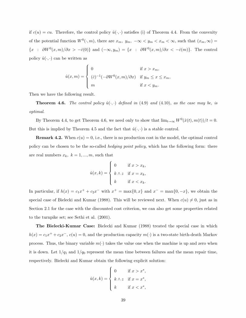
if c(u) = cu. Therefore, the control policy u(·, ·) satisfies (i) of Theorem 4.4. From the convexity
of the potential function W 0(·,m), there are xm, ym, −∞ < ym < xm < ∞, such that (xm,∞) =
x : ∂W 0(x,m)/∂x > −c(0) and (−∞, ym) = x : ∂W 0(x,m)/∂x < −c(m). The control
policy u(·, ·) can be written as
u(x, m) =
0 if x > xm,
(c)−1(−∂W 0(x,m)/∂x) if ym ≤ x ≤ xm,
m if x < ym.
Then we have the following result.
Theorem 4.6. The control policy u(·, ·) defined in (4.9) and (4.10), as the case may be, is
optimal.
By Theorem 4.4, to get Theorem 4.6, we need only to show that limt→∞W 0(x(t),m(t))/t = 0.
But this is implied by Theorem 4.5 and the fact that u(·, ·) is a stable control.
Remark 4.2. When c(u) = 0, i.e., there is no production cost in the model, the optimal control
policy can be chosen to be the so-called hedging point policy, which has the following form: there
are real numbers xk, k = 1, ..., m, such that
u(x, k) =
0 if x > xk,
k ∧ z if x = xk,
k if x < xk.
In particular, if h(x) = c1x+ + c2x
− with x+ = max0, x and x− = max0,−x, we obtain the
special case of Bielecki and Kumar (1988). This will be reviewed next. When c(u) 6= 0, just as in
Section 2.1 for the case with the discounted cost criterion, we can also get some properties related
to the turnpike set; see Sethi et al. (2001).
The Bielecki-Kumar Case: Bielecki and Kumar (1988) treated the special case in which
h(x) = c1x+ + c2x
−, c(u) = 0, and the production capacity m(·) is a two-state birth-death Markov
process. Thus, the binary variable m(·) takes the value one when the machine is up and zero when
it is down. Let 1/q1 and 1/q0 represent the mean time between failures and the mean repair time,
respectively. Bielecki and Kumar obtain the following explicit solution:
u(x, k) =
0 if x > x∗,
k ∧ z if x = x∗,
k if x < x∗,
39
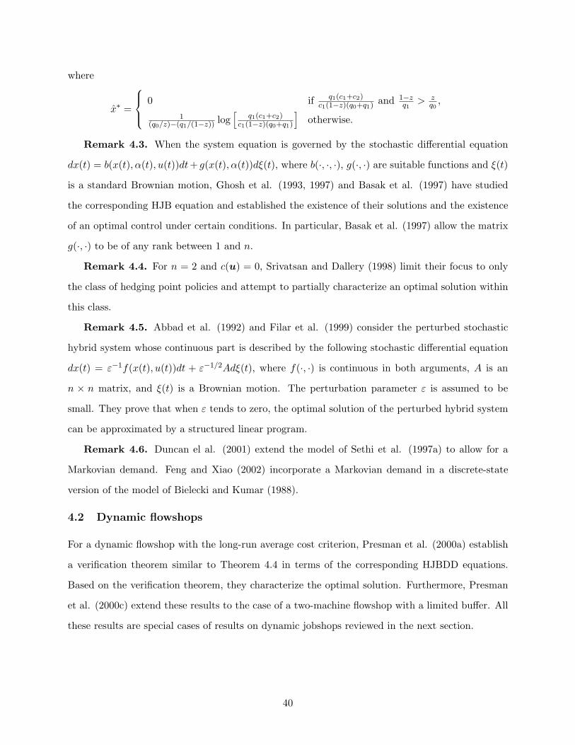
where
x∗ =
0 if q1(c1+c2)c1(1−z)(q0+q1) and 1−z
q1> z
q0,
1(q0/z)−(q1/(1−z)) log
[q1(c1+c2)
c1(1−z)(q0+q1)
]otherwise.
Remark 4.3. When the system equation is governed by the stochastic differential equation
dx(t) = b(x(t), α(t), u(t))dt+ g(x(t), α(t))dξ(t), where b(·, ·, ·), g(·, ·) are suitable functions and ξ(t)
is a standard Brownian motion, Ghosh et al. (1993, 1997) and Basak et al. (1997) have studied
the corresponding HJB equation and established the existence of their solutions and the existence
of an optimal control under certain conditions. In particular, Basak et al. (1997) allow the matrix
g(·, ·) to be of any rank between 1 and n.
Remark 4.4. For n = 2 and c(u) = 0, Srivatsan and Dallery (1998) limit their focus to only
the class of hedging point policies and attempt to partially characterize an optimal solution within
this class.
Remark 4.5. Abbad et al. (1992) and Filar et al. (1999) consider the perturbed stochastic
hybrid system whose continuous part is described by the following stochastic differential equation
dx(t) = ε−1f(x(t), u(t))dt + ε−1/2Adξ(t), where f(·, ·) is continuous in both arguments, A is an
n × n matrix, and ξ(t) is a Brownian motion. The perturbation parameter ε is assumed to be
small. They prove that when ε tends to zero, the optimal solution of the perturbed hybrid system
can be approximated by a structured linear program.
Remark 4.6. Duncan el al. (2001) extend the model of Sethi et al. (1997a) to allow for a
Markovian demand. Feng and Xiao (2002) incorporate a Markovian demand in a discrete-state
version of the model of Bielecki and Kumar (1988).
4.2 Dynamic flowshops
For a dynamic flowshop with the long-run average cost criterion, Presman et al. (2000a) establish
a verification theorem similar to Theorem 4.4 in terms of the corresponding HJBDD equations.
Based on the verification theorem, they characterize the optimal solution. Furthermore, Presman
et al. (2000c) extend these results to the case of a two-machine flowshop with a limited buffer. All
these results are special cases of results on dynamic jobshops reviewed in the next section.
40
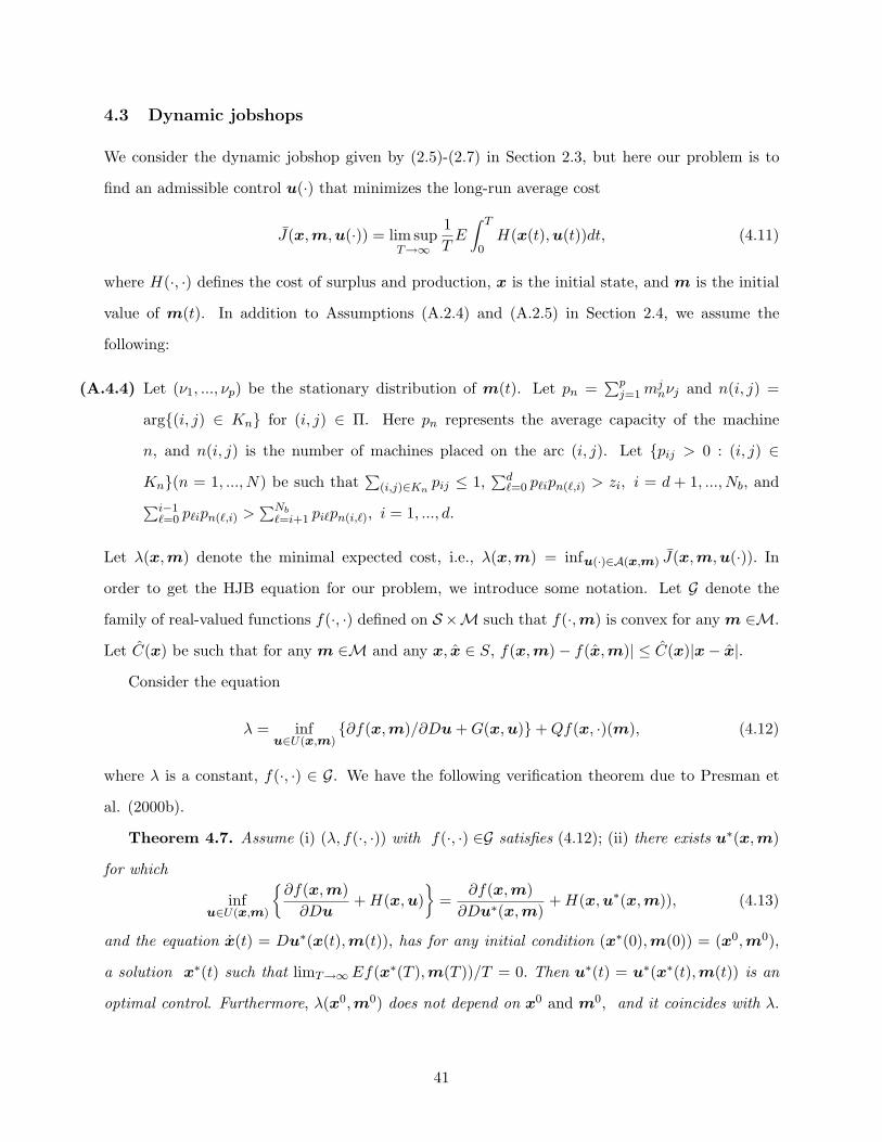
4.3 Dynamic jobshops
We consider the dynamic jobshop given by (2.5)-(2.7) in Section 2.3, but here our problem is to
find an admissible control u(·) that minimizes the long-run average cost
J(x, m,u(·)) = lim supT→∞
1T
E
∫ T
0H(x(t), u(t))dt, (4.11)
where H(·, ·) defines the cost of surplus and production, x is the initial state, and m is the initial
value of m(t). In addition to Assumptions (A.2.4) and (A.2.5) in Section 2.4, we assume the
following:
(A.4.4) Let (ν1, ..., νp) be the stationary distribution of m(t). Let pn =∑p
j=1 mjnνj and n(i, j) =
arg(i, j) ∈ Kn for (i, j) ∈ Π. Here pn represents the average capacity of the machine
n, and n(i, j) is the number of machines placed on the arc (i, j). Let pij > 0 : (i, j) ∈Kn(n = 1, ..., N) be such that
∑(i,j)∈Kn
pij ≤ 1,∑d
`=0 p`ipn(`,i) > zi, i = d + 1, ..., Nb, and∑i−1
`=0 p`ipn(`,i) >∑Nb
`=i+1 pi`pn(i,`), i = 1, ..., d.
Let λ(x, m) denote the minimal expected cost, i.e., λ(x,m) = infu(·)∈A(x,m) J(x,m, u(·)). In
order to get the HJB equation for our problem, we introduce some notation. Let G denote the
family of real-valued functions f(·, ·) defined on S ×M such that f(·, m) is convex for any m ∈M.
Let C(x) be such that for any m ∈M and any x, x ∈ S, f(x, m)− f(x, m)| ≤ C(x)|x− x|.Consider the equation
λ = infu∈U(x,m)
∂f(x, m)/∂Du + G(x, u)+ Qf(x, ·)(m), (4.12)
where λ is a constant, f(·, ·) ∈ G. We have the following verification theorem due to Presman et
al. (2000b).
Theorem 4.7. Assume (i) (λ, f(·, ·)) with f(·, ·) ∈G satisfies (4.12); (ii) there exists u∗(x, m)
for which
infu∈U(x,m)
∂f(x, m)
∂Du+ H(x, u)
=
∂f(x, m)∂Du∗(x, m)
+ H(x, u∗(x, m)), (4.13)
and the equation x(t) = Du∗(x(t), m(t)), has for any initial condition (x∗(0), m(0)) = (x0, m0),
a solution x∗(t) such that limT→∞Ef(x∗(T ),m(T ))/T = 0. Then u∗(t) = u∗(x∗(t), m(t)) is an
optimal control. Furthermore, λ(x0, m0) does not depend on x0 and m0, and it coincides with λ.
41
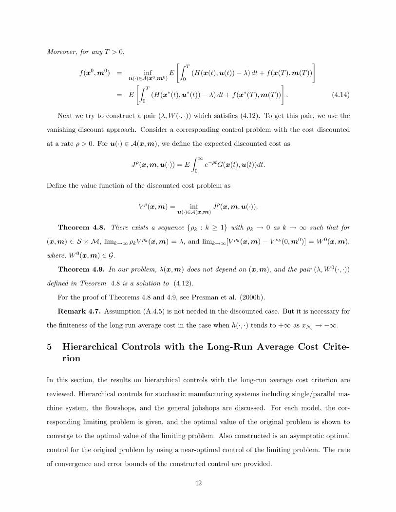
Moreover, for any T > 0,
f(x0, m0) = infu(·)∈A(x0,m0)
E
[∫ T
0(H(x(t), u(t))− λ) dt + f(x(T ), m(T ))
]
= E
[∫ T
0(H(x∗(t),u∗(t))− λ) dt + f(x∗(T ), m(T ))
]. (4.14)
Next we try to construct a pair (λ,W (·, ·)) which satisfies (4.12). To get this pair, we use the
vanishing discount approach. Consider a corresponding control problem with the cost discounted
at a rate ρ > 0. For u(·) ∈ A(x, m), we define the expected discounted cost as
Jρ(x, m, u(·)) = E
∫ ∞
0e−ρtG(x(t), u(t))dt.
Define the value function of the discounted cost problem as
V ρ(x,m) = infu(·)∈A(x,m)
Jρ(x,m, u(·)).
Theorem 4.8. There exists a sequence ρk : k ≥ 1 with ρk → 0 as k → ∞ such that for
(x, m) ∈ S ×M, limk→∞ ρkVρk(x, m) = λ, and limk→∞[V ρk(x, m) − V ρk(0, m0)] = W 0(x, m),
where, W 0(x,m) ∈ G.
Theorem 4.9. In our problem, λ(x,m) does not depend on (x, m), and the pair (λ,W 0(·, ·))defined in Theorem 4.8 is a solution to (4.12).
For the proof of Theorems 4.8 and 4.9, see Presman et al. (2000b).
Remark 4.7. Assumption (A.4.5) is not needed in the discounted case. But it is necessary for
the finiteness of the long-run average cost in the case when h(·, ·) tends to +∞ as xNb→ −∞.
5 Hierarchical Controls with the Long-Run Average Cost Crite-rion
In this section, the results on hierarchical controls with the long-run average cost criterion are
reviewed. Hierarchical controls for stochastic manufacturing systems including single/parallel ma-
chine system, the flowshops, and the general jobshops are discussed. For each model, the cor-
responding limiting problem is given, and the optimal value of the original problem is shown to
converge to the optimal value of the limiting problem. Also constructed is an asymptotic optimal
control for the original problem by using a near-optimal control of the limiting problem. The rate
of convergence and error bounds of the constructed control are provided.
42
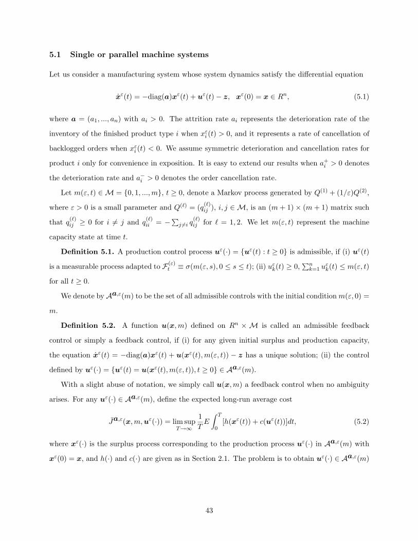
5.1 Single or parallel machine systems
Let us consider a manufacturing system whose system dynamics satisfy the differential equation
xε(t) = −diag(a)xε(t) + uε(t)− z, xε(0) = x ∈ Rn, (5.1)
where a = (a1, ..., an) with ai > 0. The attrition rate ai represents the deterioration rate of the
inventory of the finished product type i when xεi (t) > 0, and it represents a rate of cancellation of
backlogged orders when xεi (t) < 0. We assume symmetric deterioration and cancellation rates for
product i only for convenience in exposition. It is easy to extend our results when a+i > 0 denotes
the deterioration rate and a−i > 0 denotes the order cancellation rate.
Let m(ε, t) ∈M = 0, 1, ..., m, t ≥ 0, denote a Markov process generated by Q(1) + (1/ε)Q(2),
where ε > 0 is a small parameter and Q(`) = (q(`)ij ), i, j ∈ M, is an (m + 1)× (m + 1) matrix such
that q(`)ij ≥ 0 for i 6= j and q
(`)ii = −∑
j 6=i q(`)ij for ` = 1, 2. We let m(ε, t) represent the machine
capacity state at time t.
Definition 5.1. A production control process uε(·) = uε(t) : t ≥ 0 is admissible, if (i) uε(t)
is a measurable process adapted to F (ε)t ≡ σ(m(ε, s), 0 ≤ s ≤ t); (ii) uε
k(t) ≥ 0,∑n
k=1 uεk(t) ≤ m(ε, t)
for all t ≥ 0.
We denote by Aa,ε(m) to be the set of all admissible controls with the initial condition m(ε, 0) =
m.
Definition 5.2. A function u(x, m) defined on Rn × M is called an admissible feedback
control or simply a feedback control, if (i) for any given initial surplus and production capacity,
the equation xε(t) = −diag(a)xε(t) + u(xε(t), m(ε, t)) − z has a unique solution; (ii) the control
defined by uε(·) = uε(t) = u(xε(t), m(ε, t)), t ≥ 0 ∈ Aa,ε(m).
With a slight abuse of notation, we simply call u(x, m) a feedback control when no ambiguity
arises. For any uε(·) ∈ Aa,ε(m), define the expected long-run average cost
Ja,ε(x,m, uε(·)) = lim supT→∞
1T
E
∫ T
0[h(xε(t)) + c(uε(t))]dt, (5.2)
where xε(·) is the surplus process corresponding to the production process uε(·) in Aa,ε(m) with
xε(0) = x, and h(·) and c(·) are given as in Section 2.1. The problem is to obtain uε(·) ∈ Aa,ε(m)
43
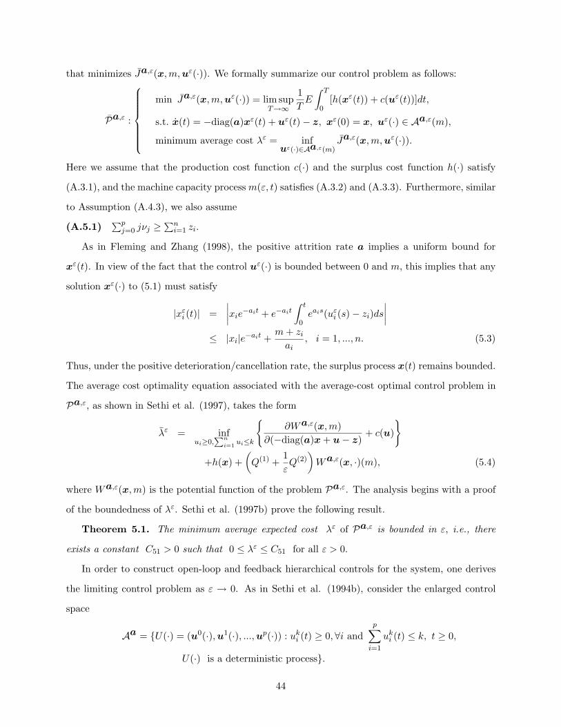
that minimizes Ja,ε(x,m, uε(·)). We formally summarize our control problem as follows:
Pa,ε :
min Ja,ε(x,m, uε(·)) = lim supT→∞
1T
E
∫ T
0[h(xε(t)) + c(uε(t))]dt,
s.t. x(t) = −diag(a)xε(t) + uε(t)− z, xε(0) = x, uε(·) ∈ Aa,ε(m),
minimum average cost λε = infuε(·)∈Aa,ε(m)
Ja,ε(x,m, uε(·)).
Here we assume that the production cost function c(·) and the surplus cost function h(·) satisfy
(A.3.1), and the machine capacity process m(ε, t) satisfies (A.3.2) and (A.3.3). Furthermore, similar
to Assumption (A.4.3), we also assume
(A.5.1)∑p
j=0 jνj ≥∑n
i=1 zi.
As in Fleming and Zhang (1998), the positive attrition rate a implies a uniform bound for
xε(t). In view of the fact that the control uε(·) is bounded between 0 and m, this implies that any
solution xε(·) to (5.1) must satisfy
|xεi (t)| =
∣∣∣∣xie−ait + e−ait
∫ t
0eais(uε
i (s)− zi)ds
∣∣∣∣
≤ |xi|e−ait +m + zi
ai, i = 1, ..., n. (5.3)
Thus, under the positive deterioration/cancellation rate, the surplus process x(t) remains bounded.
The average cost optimality equation associated with the average-cost optimal control problem in
Pa,ε, as shown in Sethi et al. (1997), takes the form
λε = infui≥0,
∑n
i=1ui≤k
∂Wa,ε(x,m)
∂(−diag(a)x + u− z)+ c(u)
+h(x) +(
Q(1) +1εQ(2)
)Wa,ε(x, ·)(m), (5.4)
where Wa,ε(x,m) is the potential function of the problem Pa,ε. The analysis begins with a proof
of the boundedness of λε. Sethi et al. (1997b) prove the following result.
Theorem 5.1. The minimum average expected cost λε of Pa,ε is bounded in ε, i.e., there
exists a constant C51 > 0 such that 0 ≤ λε ≤ C51 for all ε > 0.
In order to construct open-loop and feedback hierarchical controls for the system, one derives
the limiting control problem as ε → 0. As in Sethi et al. (1994b), consider the enlarged control
space
Aa = U(·) = (u0(·),u1(·), ...,up(·)) : uki (t) ≥ 0, ∀i and
p∑
i=1
uki (t) ≤ k, t ≥ 0,
U(·) is a deterministic process.
44
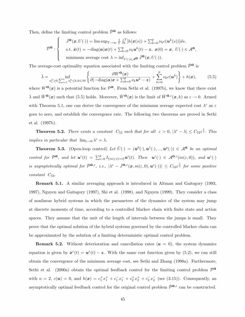
Then, define the limiting control problem Pa as follows:
Pa :
Ja(x, U(·)) = lim supT→∞1T
∫ T0 [h(x(s)) +
∑pk=0 νkc(uk(s))]ds,
s.t. x(t) = −diag(a)x(t) +∑p
k=0 νkuk(t)− z, x(0) = x, U(·) ∈ Aa,
minimum average cost λ = infU(·)∈Aa Ja(x, U(·)).The average-cost optimality equation associated with the limiting control problem Pa is
λ = infuk
i≥0,∑n
i=1uk
i≤k,k∈M
∂Wa(x)
∂(−diag(a)x +∑p
k=0 νkuk − z)+
p∑
k=0
νkc(uk)
+ h(x), (5.5)
where Wa(x) is a potential function for Pa. From Sethi et al. (1997b), we know that there exist
λ and Wa(x) such that (5.5) holds. Moreover, Wa(x) is the limit of Wa,ε(x, k) as ε → 0. Armed
with Theorem 5.1, one can derive the convergence of the minimum average expected cost λε as ε
goes to zero, and establish the convergence rate. The following two theorems are proved in Sethi
et al. (1997b).
Theorem 5.2. There exists a constant C52 such that for all ε > 0, |λε − λ| ≤ C52ε12 . This
implies in particular that limε→0 λε = λ.
Theorem 5.3. (Open-loop control) Let U(·) = (u0(·), u1(·), ..., up(·)) ∈ Aa be an optimal
control for Pa, and let uε(t) =∑p
i=0 Im(ε,t)=iui(t). Then uε(·) ∈ Aa,ε(m(ε, 0)), and uε(·)is asymptotically optimal for Pa,ε, i.e., |λε − Ja,ε(x,m(ε, 0), uε(·))| ≤ C53ε
12 for some positive
constant C53.
Remark 5.1. A similar averaging approach is introduced in Altman and Gaitsgory (1993,
1997), Nguyen and Gaitsgory (1997), Shi et al. (1998), and Nguyen (1999). They consider a class
of nonlinear hybrid systems in which the parameters of the dynamics of the system may jump
at discrete moments of time, according to a controlled Markov chain with finite state and action
spaces. They assume that the unit of the length of intervals between the jumps is small. They
prove that the optimal solution of the hybrid systems governed by the controlled Markov chain can
be approximated by the solution of a limiting deterministic optimal control problem.
Remark 5.2. Without deterioration and cancellation rates (a = 0), the system dynamics
equation is given by xε(t) = uε(t) − z. With the same cost function given by (5.2), we can still
obtain the convergence of the minimum average cost, see Sethi and Zhang (1998a). Furthermore,
Sethi et al. (2000a) obtain the optimal feedback control for the limiting control problem Pa
with n = 2, c(u) = 0, and h(x) = c+1 x+
1 + c−1 x−1 + c+2 x+
2 + c−2 x−2 (see (3.15)). Consequently, an
asymptotically optimal feedback control for the original control problem Pa,ε can be constructed.
45
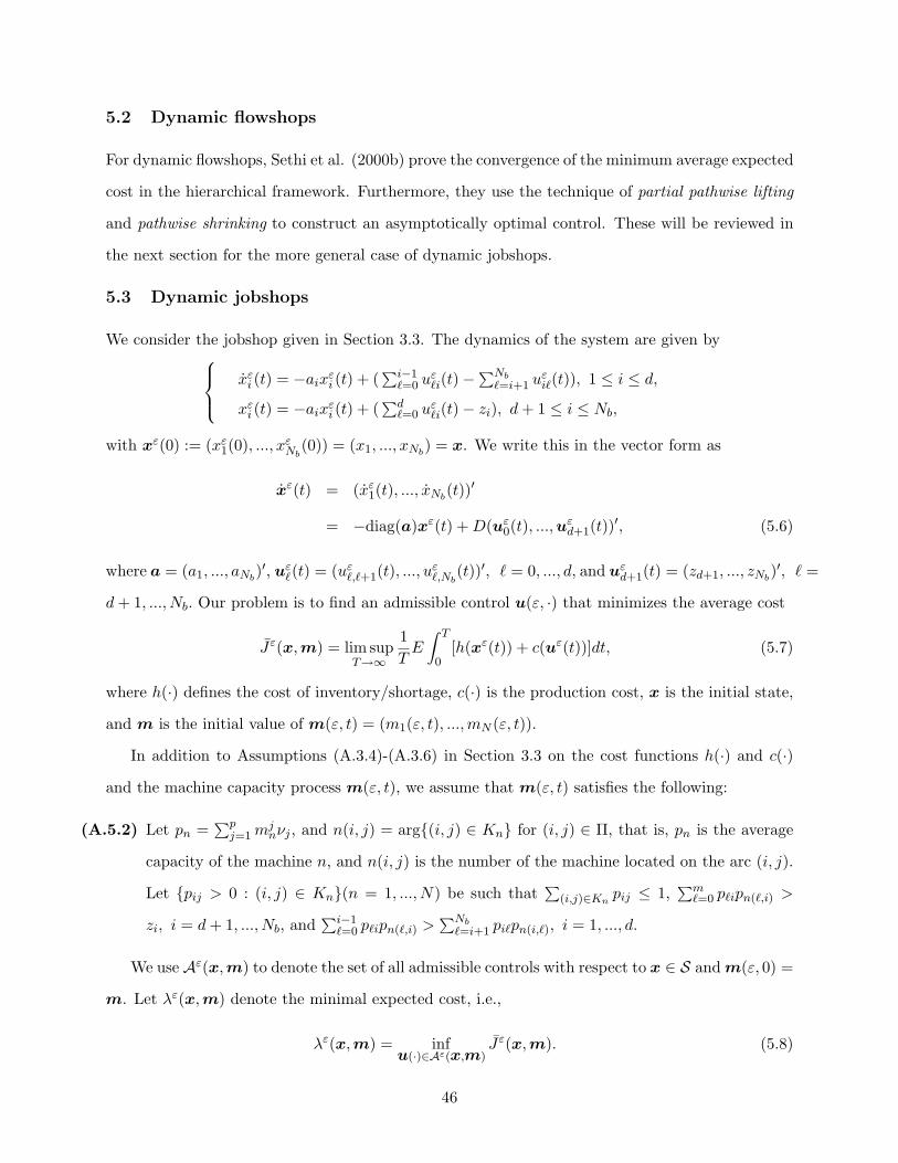
5.2 Dynamic flowshops
For dynamic flowshops, Sethi et al. (2000b) prove the convergence of the minimum average expected
cost in the hierarchical framework. Furthermore, they use the technique of partial pathwise lifting
and pathwise shrinking to construct an asymptotically optimal control. These will be reviewed in
the next section for the more general case of dynamic jobshops.
5.3 Dynamic jobshops
We consider the jobshop given in Section 3.3. The dynamics of the system are given by
xεi (t) = −aix
εi (t) + (
∑i−1`=0 uε
`i(t)−∑Nb
`=i+1 uεi`(t)), 1 ≤ i ≤ d,
xεi (t) = −aix
εi (t) + (
∑d`=0 uε
`i(t)− zi), d + 1 ≤ i ≤ Nb,
with xε(0) := (xε1(0), ..., xε
Nb(0)) = (x1, ..., xNb
) = x. We write this in the vector form as
xε(t) = (xε1(t), ..., xNb
(t))′
= −diag(a)xε(t) + D(uε0(t), ...,u
εd+1(t))
′, (5.6)
where a = (a1, ..., aNb)′, uε
`(t) = (uε`,`+1(t), ..., u
ε`,Nb
(t))′, ` = 0, ..., d, and uεd+1(t) = (zd+1, ..., zNb
)′, ` =
d + 1, ..., Nb. Our problem is to find an admissible control u(ε, ·) that minimizes the average cost
Jε(x, m) = lim supT→∞
1T
E
∫ T
0[h(xε(t)) + c(uε(t))]dt, (5.7)
where h(·) defines the cost of inventory/shortage, c(·) is the production cost, x is the initial state,
and m is the initial value of m(ε, t) = (m1(ε, t), ..., mN (ε, t)).
In addition to Assumptions (A.3.4)-(A.3.6) in Section 3.3 on the cost functions h(·) and c(·)and the machine capacity process m(ε, t), we assume that m(ε, t) satisfies the following:
(A.5.2) Let pn =∑p
j=1 mjnνj , and n(i, j) = arg(i, j) ∈ Kn for (i, j) ∈ Π, that is, pn is the average
capacity of the machine n, and n(i, j) is the number of the machine located on the arc (i, j).
Let pij > 0 : (i, j) ∈ Kn(n = 1, ..., N) be such that∑
(i,j)∈Knpij ≤ 1,
∑m`=0 p`ipn(`,i) >
zi, i = d + 1, ..., Nb, and∑i−1
`=0 p`ipn(`,i) >∑Nb
`=i+1 pi`pn(i,`), i = 1, ..., d.
We use Aε(x, m) to denote the set of all admissible controls with respect to x ∈ S and m(ε, 0) =
m. Let λε(x, m) denote the minimal expected cost, i.e.,
λε(x, m) = infu(·)∈Aε(x,m)
Jε(x,m). (5.8)
46
In the case of the long-run average cost criterion used here, we know, by Theorem 2.4 in Presman
et al. (2000b), that under Assumption (A.5.2), λε(x, m) is independent of the initial condition
(x, m). Thus we will use λε instead of λε(x, m). We use Pε to denote our control problem, i.e.,
Pε :
minimize Jε(x, m0) = lim supT→∞1T E
∫ T0 h(xε(t)) + u(uε(t))dt,
subject to
xε(t) = −diag(a)xε(t) + Duε(t), xε(0) = x,
uε(·) ∈ Aε(x,m)
value function λε = infuε(·)∈Aε(x,m0) Jε(x,m).
(5.9)
As in Section 5.1, the positive attrition rate a implies a uniform bound for xε(t). Next we examine
elementary properties of the potential function and obtain the limiting control problem as ε → 0.
The HJBDD equation, as shown in Sethi et al. (1998b, 2000c), takes the form
λε = infu∈U(x,mj)
∂Wa,ε(x, mj)
∂(−diag(a)x + Du)+ c(u)
+ h(x)
+(
Q(1) +1εQ(2)
)Wa,ε(x, ·)(mj), (5.10)
where Wa,ε(x, mj) is the potential function of the problem Pε. Moreover, following Presman et
al. (2000b), we can show that there exists a potential function Wa,ε(x, m) such that the pair
(λε,Wa,ε(x, m)) is a solution of (5.10), where λε is the minimum average expected cost for Pε.
First, we can get the boundedness of λε.
Theorem 5.4. There exists a constant M1 > 0 such that 0 ≤ λε ≤ M1 for all ε > 0.
For its proof, see Sethi et al. (2000c). Now we derive the limiting control problem as ε → 0.
As in Sethi and Zhou (1994), for x ∈ S, let A0(x) denote the set of measurable controls
U(·) = (u1(·), ...,up(·))
= ((u1,00 (·), ...,u1,0
d )(·), ..., (up,00 (·), ..., up,0
d )(·)),
with uj,0k (·) = (uj,0
k,k+1(·), ..., uj,0k,Nb
(·)), such that 0 ≤ ∑(i,j)∈Kn
uj,0ij (t) ≤ mj
n for all t ≥ 0, j = 1, ..., p,
and n = 1, ..., N , and the corresponding solutions x(·) of the system
xk(t) = −akxk(t) +(∑p
j=1 γj∑k−1
`=0 uj`k(t)−
∑pj=1 γj
∑N`=k+1 uj
k`(t))
,
k = 1, ..., d, and
xk(t) = −akxk(t) +(∑p
j=1 γj∑d
`=1 uj`k(t)− dk
), k = d + 1, ..., N,
with (x1(0), ..., xN (0)) = (x1, ..., xN ) satisfy x(t) ∈ S for all t ≥ 0.
47
The objective is to choose a control U(·) ∈ A0(x) that minimizes
J(U(·)) = lim supT→∞
1T
∫ T
0[h(x(s)) +
p∑
j=0
γjc(uj(s))]ds.
We use P0 to denote the above problem, and regard this as our limiting problem. Then we define
the limiting control problem P0 as follows:
P0 :
J(U(·)) = lim supT→∞1T
∫ T0
[h(x(s)) +
∑pj=0 γjc(uj(s))
]ds,
xk(t) = −akxk(t) +(∑p
j=1 γj∑k−1
`=0 uj`k(t)−
∑pj=1 γj
∑N`=k+1 uj
k`(t))
,
with xk(0) = xk, k = 1, ..., d, and
xk(t) = −akxk(t) +(∑p
j=1 γj∑d
`=0 uj`m(t)− dk
),
with xk(0) = xk k = d + 1, ..., N,
U(·) ∈ A0(x),
minimum average cost λ = infU(·)∈A0 J(U(·)).
The average cost optimality equation associated with the limiting control problem P0 is
λ = infU0∈A0
∂Wa(x)∂(−diag(a)x + DU0)
+p∑
j=0
γjc(uj)
+ h(x), (5.11)
where Wa(x) is a potential function for P0 and U0 =∑p
j=1 γjuj . From Presman et al. (2000b),
we know that there exist λ and Wa(x) such that (5.11) holds. Moreover, Wa(x) is the limit of
Wa,ε(x, m) as ε → 0. The following convergence result for the minimum average expected cost
λε, as ε goes to zero, is established in Sethi et al. (2000c).
Theorem 5.5. For any δ ∈ [0, 12) there exists a constant C56 > 0 such that for all sufficiently
small ε > 0, |λε − λ| ≤ C56εδ. This implies in particular that limε→0 λε = λ.
5.4 Markov decision processes with weak and strong interactions
Markovian decision processes (MDP) have received much attention in recent years because of their
capability in dealing with a large class of practical problems under uncertainty. The formulation
of many practical problems, such as queueing and machine replacement, fits well in the framework
of Markov decision processes; see Derman (1970). In this section we present results that provide
a justification for hierarchical controls of a class of Markov decision problems. We focus on the
problem of a finite state continuous-time Markov decision process that has both weak and strong
interactions. More specifically, the state of the process can be divided into several groups such that
48
transitions among the states within each group occur much more frequently than the transitions
among the states belonging to different groups. By replacing the states in each group by the
corresponding average distribution, we can derive a limiting problem which is simpler to solve.
Given an optimal solution to limiting problem, we can construct a solution for the original problem
which is asymptotically optimal. Proofs of results in this section can be found in Zhang (1996).
Let us consider a Markov decision process x(·) = x(t) : t ≥ 0 and a control process u(·) =
u(t) = u(x(t)) : t ≥ 0 such that u(t) ∈ U , t ≥ 0, where U is a set with finite elements. Let
Qε(u(t)) = (qεij(u(t))), t ≥ 0, denote the generator of x(·) such that Qε(u) =
1εA(u) + B(u), where
A(u) = diagA1(u), . . . , Ar(u), Ak(u) = (akij(u))pk×pk
with akij(u) ≥ 0 for j 6= i and
∑j ak
ij(u) = 0,
B(u) = (bij(u))p×p with p = p1 + · · ·+ pr, bij(u) ≥ 0 for j 6= i and∑
j bij(u) = 0, and ε is a small
parameter. For each k = 1, . . . , r, let Mk = sk1, . . . , skpk, where pk is the dimension of Ak(u).
The state space of x(·) is given by M = M1 × . . .×Mr, i.e.,
M = s11, . . . , s1p1 , s21, . . . , s2p2 , . . . , sr1, . . . , srpr.
The matrix A(u) dictates the fast transition of the process x(·) within each group Mk, k =
1, . . . , r, and the matrix B(u) together with the average distribution of the Markov chain generated
by Ak(u) dictates the slow transition of x(·) between different groups. When ε is small, the process
x(·) has a strong interaction within any group Mk, k = 1, . . . , r, and has a weak interaction among
these groups. Let u = u(i) denote a function such that u(i) ∈ U for all i ∈ M. We call u an
admissible control and use Υ to denote all such functions. For each k = 1, . . . , r, let
Γk = Uk := (uk1, . . . , ukpk) : such that ukj ∈ U, j = 1, . . . , pk.
The control set for the limiting problem is defined as Γ = Γ1 × · · · × Γr, i.e.,
Γ = U = (U1, . . . , U r) = (u11, . . . , u1p1 , . . . , ur1, . . . , urpr)
: such that Uk ∈ Γk, k = 1, . . . , r.
We define matrices Ak, B, and Qε as follows. For each U = (U1, . . . , U r) ∈ Γ, let Ak(Uk) =
49
(akij(ski, u
ki)), k = 1, . . . , r, B(U) = (bij(U)) where
bij(U) =
bij(u1i) if 1 ≤ i ≤ p1,
bij(u2(i−p1)) if p1 + 1 ≤ i ≤ p1 + p2,
· · · · · ·bij(ur(i−p+pr)) if p− pr + 1 ≤ i ≤ p.
with p = p1 + · · ·+ pr, and
Qε(U) =1εdiag
A1(U1), . . . , Ar(U r)
+ B(U). (5.12)
For each Uk ∈ Γk, let νk(Uk) denote the average distribution of the Markov chain generated by
Ak(Uk) for k = 1, . . . , r. Define ν(U) = diagν1(U1), . . . , νr(U r) and Ie = diagep1 , . . . , epr with
epk= (1, . . . , 1)′ being pk dimensional column vector. Using ν(U) and Ie, we define another matrix
Q(U) as a function of U ∈ Γ:
Q(U) = ν(U)B(U)Ie. (5.13)
Note that the kth row of Q(U) depends only on Uk. Thus, Q(U) = (qij(U i))r×r. We write, with
an abuse of notation, Q(Uk)f(·)(k) =∑
k′ 6=k qkk′(Uk)(f(k′) − f(k)) instead of Q(U)f(·)(k), for a
function f defined on 1, . . . , r. We assume the following:
(A.5.3) For each U ∈ Γ, U is a finite set, Ak(Uk) is irreducible, k = 1, . . . , r, and for each ε > 0,
Qε(U) is irreducible, where Qε(U) is defined in (5.12).
We consider the following problem:
Pε :
minimize Jε(u) = lim supT→∞
1T
E
∫ T
0G(x(t), u(x(t)))dt,
subject to x(t) ∼ Qε(u(t)), x(0) = i, u ∈ Υ,
value function λε = infu∈Aε
Jε(u).
(5.14)
Note that the average cost function is independent of the initial value x(0) = i, and so is the value
function. The dynamic programming (DP) equation for Pε is
λε = minu∈U
G(i, u) + Qε(u)W ε(·)(i) , (5.15)
where W ε(·) is a function defined on M.
50
Theorem 5.6. (i) For each fixed ε > 0, there exists a pair (λε,W ε(·)) that satisfies the DP
equation (5.15).
(ii) The DP equation (5.15) has a unique solution in the sense that for any other solution
(λε, W ε(·)) to (5.15), λε = λε and W ε(·) = W ε(·) + K for some constant K.
(iii) Let u∗ε = u∗ε(i) ∈ U denote a minimizer of the right-hand side of (5.15). Then u∗ε(i) ∈ Aε
is optimal, i.e., Jε(u∗ε) = λε.
Motivated by Sethi and Zhang (1994a), we next define the limiting problem. For Uk ∈ Γk,
define G(k, Uk) =∑mk
j=1 νkj (Uk)G(skj , u
kj), k = 1, . . . , r, where νk(Uk) = (νk1 (Uk), . . . , νk
mk(Uk))
is the average distribution of the Markov chain generated by Ak(Uk). Let A0 denote a class of
functions U = U(k) ∈ Γk, k = 1, . . . , r. For convenience, we will call U = (U(1), . . . , U(r)) ∈ A0,
an admissible control for the limiting problem P0 defined below:
P0 :
minimize J0(U) = lim supT→∞
1T
E
∫ T
0G(x(t), U(x(t)))dt,
subject to x(t) ∼ Q(U(x(t))), x(0) = k, U ∈ A0,
value function λ0 = infU∈A0
J0(U).
(5.16)
It can be shown that Q(U) is irreducible for each U ∈ Γ. The DP equation for P0 is
λ0 = minUk∈Γk
G(k, Uk) + Q(Uk)W 0(·)(k)
, (5.17)
for some function W 0(·).Theorem 5.7. (i) There exists a pair (λ0,W 0(·)) that satisfies the DP equation (5.17).
(ii) The DP equation (5.17) has a unique solution in the sense that for any other solution
(λ0, W 0(·)) to (5.17), λ0 = λ0 and W 0(·) = W 0(·) + K for some constant K.
(iii) Let U∗ ∈ Γ denote a minimizer of the right-hand side of (5.17). Then U∗ ∈ A0 is optimal,
i.e., J0(U∗) = λ0.
Remark 5.3. Note that the number of the DP equations for Pε is equal to p = p1 + · · ·+ pr,
while the number of those for P0 is only r. Since for each k = 1, . . . , r, pk ≥ 2, it follows that
p − r ≥ r. The difference between p and r could be very large for either large r or a large pk for
some k. Since the computational effort involved in solving the DP equations depends in part on
the number of the equations to be solved (see Hillier and Lieberman (1989)), the effort in solving
the DP equations for P0 is substantially less than that of solving Pε for (p− r) large.
51
Insight 5.1. In the presence of states with weak and strong interactions, a near-optimal
control of the original problem can be constructed from the solution of an approximate problem
with reduced number of states, each of which is formed by aggregating the original states within
a group using the stationary distribution of these states given the reduced state corresponding to
the group.
We construct a control uε as follows:
uε = uε(x) =r∑
k=1
pk∑
j=1
Ix=skjukj∗ , (5.18)
where IA is the indicator of a set A.
Theorem 5.8. Let U∗ ∈ A0 denote an optimal control for P0 and let uε ∈ Aε be the corre-
sponding control constructed as in (5.18). Then, uε is asymptotically optimal and with error bound
ε, i.e., Jε(uε)− λε = O(ε).
Remark 5.4. Filar et al. (1999) introduce diffusions in these models; see Remark 4.5. In
their model, all jumps are associated with a slow process, while the continuous part including the
diffusions is associated with a small parameter ε (see Remark 4.5) representing a fast process. As ε
tends to zero, the problem is shown to reduce to a structured linear program. Its optimal solution
can then be used as an approximation to the optimal solution of the original system associated
with a small ε.
5.5 Single or parallel machine systems with risk-sensitive average cost criterion
Consider a single product, single/parallel machine manufacturing system described in Subsection
5.1 with the objective of minimizing the risk-sensitive average cost criterion over an infinite horizon.
Then, the objective is to choose uε(·) ∈ Aa,ε(m) so as to minimize
Jε(uε(·)) = lim supT→∞
ε
Tlog
[E exp
(1ε
∫ T
0[h(xε(t)) + c(uε(t))] dt
)], (5.19)
where xε(·) is the surplus process corresponding to the production process uε(·). Let λε =
infuε(·)∈Aa,ε(m) Jε(uε(·)). Fleming and Zhang (1998) establish the verification theorem in terms
of a viscosity solution, and give an asymptotically optimal control.
52
6 Extensions and Concluding Remarks
In this paper, we have reviewed various models of manufacturing systems consisting of flexible
machines for which a theory of optimal control has been developed and for which hierarchical
controls that are asymptotically optimal have been constructed. We have examined systems with
random production capacity and/or demand under various configurations including jobshops and
multiple hierarchical decision levels. We have considered different performance criteria such as
discounted costs, long-run average costs, risk-sensitive controls with discounted costs, and risk-
sensitive controls with average costs.
While asymptotic optimal controls have been constructed for these systems under fairly general
conditions, many problems remain open. We shall now describe some of them.
All of the results on the hierarchical controls in this survey assume the costs of inventory/shortage
and of production to be separable. Lehoczky et al. (1991) assume a nonseparable cost and prove
that the value function of the original problem converges to the value function of the limiting
problem. Controls are constructed and are only conjectured to be asymptotically optimal.
With regards to systems with state constraints such as flowshops and jobshops discussed in
Sections 3 and 5, respectively, only asymptotic optimal open-loop controls are constructed in gen-
eral. Because of the absence of the Lipschitz property of the constructed feedback controls, their
asymptotic optimality is much harder to establish. It has only been done in Sethi and Zhou (1996a,
b) and Fong and Zhou (1996, 1997) for two-machine flowshops with a specific cost structure given
in (3.15). Generalization of their results to jobshops and to general cost functions represents a
challenging research problem.
When the Markov processes involved depend on control variables, as they do in Soner (1993),
Sethi and Zhang (1994c, 1995a), and Yin and Zhang (1997), no error bounds are available for
constructed asymptotic optimal controls. Estimation of these errors and extensions of the results
to Markov processes depending as well on the state variables remain open problems.
In the case of the long-run average cost criterion, with the exception of single/parallel machine
systems in Section 5.1, we have constructed open-loop hierarchical controls only in presence of an
attrition rate. Extensions of these results to systems without an attrition term remain open. No
hierarchical feedback controls that are optimal have been constructed. In case of optimal control
53
of these ergodic systems, verification theorems have been obtained, but the existence of optimal
controls is proved only in the single product case of Section 4.1. In other cases, even the existence
of optimal controls remains an open issue.
An important class of manufacturing systems consists of systems that have machines which
are not completely flexible, and thus involve setup costs and/or setup times, when switching from
production of one product to that of another. Such systems have been considered by Gershwin
(1986), Gershwin et al. (1988), Sharifnia et al. (1991), Caramanis et al. (1991), Connolly et
al. (1992), Hu and Caramanis (1992), and Srivatsan and Gershwin (1990). They have examined
various possible heuristic policies and have carried out numerical computations and simulations.
They have not studied their policies from the viewpoint of asymptotic optimality. Sethi and Zhang
(1995b) have made some progress in this direction.
Based on the theoretical work on hierarchical control of stochastic manufacturing systems,
Srivatsan (1993) and Srivatsan et al. (1994) have developed a hierarchical framework and describe
its experimental implementation in a semiconductor research laboratory at MIT. It is expected
that such research would lead to the development of real-time decision making algorithms suitable
for use in actual flexible manufacturing facilities; see also Caramanis and Sharifnia (1991).
Finally, while error bounds have been obtained only in some cases, they do not provide informa-
tion on how small ε, the rate of slow and fast rates, have to be for asymptotic hierarchical controls
to be acceptable in practice. This issue can only be investigated computationally, and that was
done by Samaratunga et al. (1997) only for a two-machine flowshop. From a practical viewpoint,
it is important to perform such investigations for dynamic jobshops.
References
[1] Abbad, M., T. R. Bielecki, J. A. Filar. 1992. Perturbation and stability theory for Markov
control problems. IEEE Trans. Auto. Contr. 37 1421-1425.
[2] Adiri, I., A. Ben-Israel. 1966. An extension and solution of Arrow-Karlin type production models
by the pontryagin maximum principle. Cahiers du Center d’Etudes de Recherche Operationnelle.
8 147-158.
54
[3] Akella, R., P. R. Kumar. 1986. Optimal control of production rate in a failure-prone manufac-
turing system. IEEE Trans. Auto. Contr. AC-31 116-126.
[4] Altman, E., V. Gaitsgory. 1993. Control of a hybrid stochastic system. Systems Control Letters.
20 307-314.
[5] Altman, E., V. Gaitsgory. 1997. Asymptotic optimization of a nonlinear hybrid system governed
by a Markov decision process. SIAM J. Contr. Optim. 35 2070-2085.
[6] Ari, E. A., S. Axsater. 1988. Disaggregation under uncertainty in hierarchical production plan-
ning. European Journal of Operational Research. 35 182-186.
[7] Arrow, K.J., S. Karlin, H. Scarf. 1958. Studies in mathematical theory of inventory and produc-
tion. Stanford University Press, Stanford, CA.
[8] Auger, P. 1989. Dynamics and thermodynamics in hierarchically organized systems. Pergamon
Press, Oxford, England.
[9] Bai, B. 1991. Scheduling Manufacturing Systems with Work-in-Process Inventory Control. Ph.D.
Thesis, MIT Operations Research Center, Cambridge, MA.
[10] Bai, S., S. B. Gershwin. 1990. Scheduling manufacturing systems with work-in-process inven-
tory. Proc. of the 29th IEEE Conference on Decision and Control. Honolulu, HI, 557-564.
[11] Basak, G. B., A. Bisi, M. K. Ghosh. 1997. Controlled random degenerate diffusions under
long-run average cost. Stochastic and Stochastic Reports. 61 121-140.
[12] Bensoussan,S., M. Crouhy, J.-M. Proth. 1983. Mathematical Theory of Production Planning.
North-Holland, New York, NY.
[13] Bensoussan, S., S. P. Sethi, R. Vickson, N. A. Derzko. 1984. Stochastic production planning
with production constraints. SIAM J. Contr. Optim. 22 920-935.
[14] Bielecki, T. R., P. R. Kumar. 1988. Optimality of zero-inventory policies for unreliable manu-
facturing systems. Operations Research. 36 532-546.
[15] Bitran, G., E. A. Hass, K. Matsuo. 1986. Production lanning of style goods with high set-up
costs and forecast revisions. Operations Research. 34 226-236.
55
[16] Bitran, G., A. Hax. 1977. On the design of hierarchical production planning systems. Decision
Sciences. 8 28-54.
[17] Bitran, G., D. Tirupati. 1983. Hierarchical production planning. Chapter 10 in Logistics of
Production and Inventory, S. C. Graves, A. H. G. Rinnooy Kan, and P. H. Zipkin (Eds.), Vol.4
in the Series Handbooks in Operations Research and Management Science, North-Holland, Am-
sterdam, 523-568.
[18] Boukas, E. K. 1991. Techniques for flow control and preventive maintenance in manufacturing
systems. Control and Dynamic Systems. 48 327-366.
[19] Boukas, E. K., A. Haurie. 1990. Manufacturing flow control and preventive maintenance: A
stochastic control approach. IEEE Trans. on Automatic Control. 35 1024-1031.
[20] Boukas, E. K., Q. Zhang, Q. Zhou. 1993. Optimal production and maintenance planning of
flexible manufacturing systems. Proc. of the 32nd IEEE Conference on Decision and Control.
San Antonio, TX, 15-17.
[21] Boukas, E. K., Q. Zhu, Q. Zhang. 1994. A piecewise deterministic Markov process model
for flexible manufacturing systems with preventive maintenance. J. Optimization Theory and
Applications. 82 269-286.
[22] Bukh, P. N. 1992. A bibliography of hierarchical production planning techniques, methodology,
and applications (1974-1991). Technical Report, Institute of Management, University of Aarhus,
Aarhus, Demark.
[23] Caramanis, M., G. Liberopoulos. 1992. Perturbation analysis for the design of flexible manu-
facturing system flow controllers. Operations Research. 40 1107-1125.
[24] Caramanis, M., A. Sharifnia. 1991. Optimal manufacturing flow controller design. Int. J. Flex.
Manuf. Syst. 3 321-336.
[25] Caramanis, M., A. Sharifnia, J. Hu, S. B. Gershwin. 1991. development of a science base for
planning and scheduling manufacturing systems. Proc. of the 1991 NSF Design and Manufac-
turing Systems Conference, The University of Texas at Austin, Austin, TX, 27-40.
56
[26] Chen, H., A. Mandelbaum. 1994. Hierarchical modeling of stochastic networks, part I: Fluid
models, Part II: Strong approximations. in Stochastic Modeling and Analysis of Manufacturing
Systems, D. D. Yao(ed.), Springer Series in Operations Research, Springer-Verlag, New York,
NY.
[27] Cheng, S. W. 1999. Complexity science and systems engineering. J. Management Sciences in
China. 2 1-7.
[28] Committee on the Next Decade in Operations Research. 1988. Operations research: the next
decade. Operations Research. 36 619-637.
[29] Connolly, S., Y. Dallery, S. B. Gershwin. 1992. A Real-time policy for performing setup changes
in a manufacturing system. Proc. of the 31st IEEE-CDC. Tucson, AZ, 16-18.
[30] Darakananda, B. 1989. Simulation of Manufacturing Process under a Hierarchical Control
Algorithm. M.S. Thesis, MIT Department of EECS, Cambridge, MA.
[31] Davis, M. H. A. 1993. Markov Models and Optimization, Chapman & Hall, New York.
[32] Derman, C. 1970. Finite State Markovian Decision Processes. Academic Press, New York, NY.
[33] Duncan, T.E., B. Pasik-Duncan, L. Stettner. 2001. Average Cost Per Unit Time Control of
Stochastic Manufacturing Systems: Revisited. Mathematical Methods of Operations Research.
54 259-278.
[34] Feng, Y.Y., B.C. Xiao. 2002. Optimal Threshold Control in Discrete Failure-Prone Manufac-
turing Systems. IEEE Transaction on Automatic Control (to appear).
[35] Feng, Y.Y., H. Yan. 2000. Optimal production control in a discrete manufacturing system
with unreliable machines and random demands. IEEE Transactions on Automatic Control, 35
2280-2296.
[36] Filar, J. A., A. Haurie, F. Moresino, J. P. Vial. 1999. Singularly perturbed hybrid systems
approximated by structured linear programs. Proceedings of International Workshop on Markov
Processes and Controlled Markov Chains, Changsha, Hunan, China.
57
[37] Fleming, W. H.(Chair). 1988. Future directions in control theory: A mathematical perspective.
SIAM Reports on Issues in the Mathematical Sciences, Philadelphia, PA.
[38] Fleming, W. H., W. M. McEneaney. 1995. Risk-sensitive control on an infinite horizon. SIAM
J. Contr. Optim. 33 1881-1921.
[39] Fleming, W. H., S. P. Sethi, M. Soner. 1987. An optimal stochastic production planning
problem with random fluctuating demand. SIAM J. Contr. Optim. 25 1494-1502.
[40] Fleming, W. H., M. Soner. 1992. Controlled Markov Processes and Viscosity Solutions.
Springer-Verlag, New York.
[41] Fleming, W. H., Q. Zhang. 1998. risk-sensitive production planning of a stochastic manufac-
turing system. SIAM J. Contr. Optim. 36 1147-1170.
[42] Fong, N. T., X. Y. Zhou. 1996. Hierarchical production policies in stochastic two-machine
flowshop with finite buffers. Journal of Optimization Theory and Applications. 89 681-712.
[43] Fong, N. T., X. Y. Zhou. 1997. Hierarchical production policies in stochastic two-machine
flowshop with finite buffers II: Feedback controls. Working Paper, Department of Systems Engi-
neering and Engineering Management, Chinese University of Hong Kong.
[44] Gelders, L. G., L. Van Wassenhove. 1981. Production planning: a review. European Journal
of Operational Research. 7 101-110.
[45] Gershwin, S. B. 1986. Stochastic scheduling and setups in a flexible manufacturing system.
Proc. of Second ORSA/TIMS Conference on Flexible Manufacturing Systems. Ann Arbor, MI,
431-442.
[46] Gershwin, S. B. 1989. Hierarchical flow control: a framework for scheduling and planning
discrete events in manufacturing systems. Proceedings of the IEEE, Special Issue on Dynamics
of Discrete Event Systems. 77 195-209.
[47] Gershwin, S. B., R. Akella, Y. Choong. 1985. Short term production scheduling of an auto-
mated manufacturing facility. IBM J. Res. Dev. 29 392-400.
58
[48] Gershwin, S. B., M. Caramanis, P. Murray. 1988. Simulation experience with a hierarchical
scheduling policy for a simple manufacturing system. Proceedings of the 27th IEEE Conference
on Decision and Control, Austin, TX, 3 1841-1849.
[49] Gfrerer, H., G. Zapfel. 1994. Hierarchical model for production planning in the case of uncertain
demand. Working Paper, Johannes Kepler Universitat Linz, Linz, Austria.
[50] Ghosh, M. K., A. Arapostathis, S. I. Marcus. 1993. Optimal control of switching diffusions
with applications to flexible manufacturing systems. SIAM J. on Contr. Optim. 31 1183-1204.
[51] Ghosh, M. K., A. Arapostathis, S. I. Marcus. 1997. Ergodic control of switching diffusions.
SIAM J. on Contr. Optim. 35 1952-1988.
[52] Harrison, M., M. I. Taksar. 1983. Instantaneous control of Brownian motion. Mathematics of
Operations Research. 8 439-453.
[53] Harrison, M., T. M. Sellke, A. J. Taylor. 1983. Impulse control of Brownian motion. Mathe-
matics of Operations Research. 8 454-466.
[54] Harrison, M., L. M. Wein. 1989. Scheduling networks of queues: heavy traffic analysis of a
simple open network. Queuing Systems: Theory and Applications. 5 265-280.
[55] Harrison, M., L. M. Wein. 1990. Scheduling networks of queues: heavy traffic analysis of a
two-station closed network. Operations Research. 38 1052-1064.
[56] Hartl, R. F., S. P. Sethi. 1984. Optimal control problems with differential inclusions: sufficiency
conditions and an application to a production-inventory model. Optimal Control Applications &
Methods. 5 289-307.
[57] Hartman, P. 1982. Ordinary Differential Equations. 2nd Edition, Birkhauser-Verlag, Boston,
MA.
[58] Hax, A. C., D. Candea. 1984. Production and Inventory Management. Prentice-Hall, Engle-
wood Cliffs, NJ.
[59] Hillier, F. S., G. L. Lieberman. 1989. Introduction to Operations Research. McGraw-Hill, New
York, NY.
59
[60] Holt, C. C., F. Modigliani, J. F. Muth, H. A. Simon. 1960. Planning Production, Inventories,
and Workforce. Prentice-Hall, Inc. Englewood Cliffs, NJ.
[61] Hu, J., M. Caramanis. 1992. Near optimal setup scheduling for flexible manufacturing systems.
Proc. of the Third RPI International Conference on Computer Integrated Manufacturing. Troy,
NY.
[62] Jiang, J., S. P. Sethi. 1991. A state aggregation approach to manufacturing systems having
machines states with weak and strong interactions. Operations Research. 39 970-978.
[63] Johnson, S. M. 1957. Sequential production planning over time at minimum cost. Management
Science. 3 435-437.
[64] Khasminskii, R. Z., G. Yin, Q. Zhang. 1997. Constructing asymptotic series for probability of
Markov chains with weak and strong interactions. Quart. Appl. Math. 38 177-200.
[65] Kimemia, J., S. B. Gershwin. 1983. An algorithm for the computer control production in
flexible manufacturing systems. IIE Trans. 15 353-362.
[66] Krichagina, E., S. Lou, S. P. Sethi, M. I. Taksar. 1993. Production control in a failure-prone
manufacturing system: diffusion approximation and asymptotic optimality. The Annals of Ap-
plied Probability. 3 421-453.
[67] Krichagina, E., S. Lou, M. I. Taksar. 1994. Double band polling for stochastic manufacturing
systems in heavy traffic. Mathematics of Operations Research. 19 560-596.
[68] Kumar, S., P. R. Kumar. 1994. Performance bounds for queuing networks and scheduling
policies. IEEE Trans. Automatic Control. 39 1600-1611.
[69] Kushner, H. J., K. M. Ramachandran. 1989. Optimal and approximately optimal control
policies for queues in heavy traffic. SIAM Journal on Control and Optimization. 27 1293-1381.
[70] Lasserre, J. B., C. merce. 1990. Robust hierarchical production planning under uncertainty.
Annals of Operations Research. 26 73-87.
60
[71] Lehoczky, J., S. P. Sethi, H. M. Soner, M. I. Taksar. 1991. An asymptotic analysis of hier-
archical control of manufacturing systems under uncertainty. Mathematics Operations Research.
16 596-608.
[72] Liberopoulos, G., M. Caramanis. 1995. Dynamics and design of a class of parameterized man-
ufacturing flow controllers. IEEE Trans. Automatic Control. 40 201-272.
[73] Liberopoulos, G., J. Hu. 1995. On the ordering of optimal hedging points in a class of manu-
facturing flow control models. IEEE Trans. Automatic Control. 40 282-286.
[74] Libosvar, C. M.. 1988. Hierarchies in production management and control: a survey. Technical
Report, LIDS-P-1734, Lab. for Infor. and Decision Systems, MIT, Cambridge, MA.
[75] Lieber, Z. 1973. An extension of Modigliani and Hohn’s planning horizons results. Management
Science. 20 319-330.
[76] Lou, S., P. Kager. 1989. A robust production control policy for VLSI wafer fabrication. IEEE
Trans. on Semiconductor Manufacturing. 2 159-164.
[77] Lou, S., S. P. Sethi, Q. Zhang. 1994. Optimal feedback production planning in a stochastic
two machine flowshop. European Journal of Operational Research–Special Issue on Stochastic
Control Theory and Operational Research. 73 331-345.
[78] Lou, S., G. van Ryzin. 1989. Optimal control rules for scheduling job shops. Annals of Opera-
tions Research. 17 233-248.
[79] Mesarovic, M., D. Macko, Y. Takahara. 1970. Theory of Multilevel Hierarchical Systems. Aca-
demic, New York, NY.
[80] Modigliani, F., F. Hohn. 1955. Production planning over time and the nature of the expectation
and planning horizon. Econometrica. 23 46-66.
[81] Nagi, R. 1991. Design and Operation of Hierarchical Production Management Systems. PH.D.
Thesis, System Research Center, University of Maryland, Baltimore, MD.
61
[82] Nguyen, M. T. 1999. Singular Perturbations in Deterministic and Stochastic Hybrid Control
Systems: An Averaging Approach. Doctoral Dissertation, University of South Australia, Adelaide,
Australia.
[83] Nguyen, M. T., V. Gaitsgory. 1997. asymptotic optimization for a class of nonlinear stochastic
hybrid systems on infinite time horizon. Proceedings of the 1997 American Control Conference,
3587-3591.
[84] Presman, E., S. P. Sethi, W. Suo. 1997a. Optimal feedback production planning in stochastic
dynamic jobshops. Mathematics of Stochastic Manufacturing Systems, Proceedings of the 1996
AMS-SIAM Summer Seminar in Applied Mathematics, G. Yin and Q. Zhang(Eds.), Lectures in
Applied Mathematics, American Mathematical Society, Providence, RI, 235-252.
[85] Presman, E., S. P. Sethi, W. Suo. 1997b. Optimal feedback production planning in a stochastic
N -machine flowshop with limited buffers. Automatica. 33 1899-1903.
[86] Presman, E., S. P. Sethi, H. Zhang, Q. Zhang. 1998. Optimality of zero-inventory policies for
an unreliable manufacturing system producing two part types. Dynamics of Continuous, Discrete
and Impulsive Systems. 4 485-496.
[87] Presman, E., S. P. Sethi, H. Zhang. 2000a. Optimal production planning in a N -machine
flowshop with long-run average cost. Mathematics and Its Applications to Industry, Edited by S.
K. Malik, Indian National Science Academy, New Delhi, 121-140.
[88] Presman, E., S. P. Sethi, H. Zhang. 2000b. Optimal production planning in stochastic jobshops
with long-run average cost. Optimization, Dynamics, and Economic Analysis, Essays in Honor
of Gustav Feichtinger, E. J. Dockner, R. F. Hartl, M. Luptacik, and G. Sorger (Eds.), Physica-
Verlag, Heidelberg, New York, 259-274.
[89] Presman, E., S. P. Sethi, H. Zhang, A. Bisi. 2000c. Optimality in two-machine flowshop with
limited buffer. Annals of Operations Research. 98 333-351.
[90] Presman, E., S. P. Sethi, Q. Zhang. 1993. Optimal feedback production planning in a stochastic
N−machine flowshop. Proc. of 12th World Congress of International Federation of Automatic
Control, Sydney, Australia.
62
[91] Presman, E., S. P. Sethi, Q. Zhang. 1995. Optimal feedback production planning in a stochastic
N-machine flowshop. Automatica. 31 1325-1332.
[92] Rogers, D. F., J. R. Evans, R. D. Plante, R. T. Wong. 1991. Aggregation and disaggregation
techniques and methodology in optimization. Operations Research. 39 553-582.
[93] Saksena, V. R., J. O’Reilly, P. Kokotovic. 1984. Singular perturbations and time-scale methods
in control theory: survey 1976-1983. Automatica. 20 273-293.
[94] Samaratunga, C., S. P. Sethi, X. Y. Zhou. 1997. Computational evaluation of hierarchical
production control policies for stochastic manufacturing systems. Operations Research. 45 258-
274.
[95] Sethi, S. P. 1997. Some insights into near-optimal plans for stochastic manufacturing systems.
Mathematics of Stochastic Manufacturing Systems, G. Yin and Q. Zhang(Eds.), Lectures in
Applied Mathematics, Vol. 33, American Mathematical Society, Providence, RI, 287-315.
[96] Sethi, S. P., H. M. Soner, Q. Zhang, J. Jiang. 1992a. Turnpike sets and their analysis in
stochastic production planning problems. Mathematics of Operations Research. 17 932-950.
[97] Sethi, S. P., W. Suo, M.I. Taksar, H. Yan. 1998a. Optimal production planning in a multi-
product stochastic manufacturing system with long-run average cost. J. Discrete Event Dynamic
Syst. 8 37-54.
[98] Sethi, S. P., W. Suo, M.I. Taksar, Q. Zhang. 1997a. Optimal production planning in a stochastic
manufacturing system with long-run average cost. Journal of Optimization Theory and Applica-
tions. 92 161-188.
[99] Sethi, S. P., M. I. Taksar, Q. Zhang. 1992b. Capacity and production decisions in stochastic
manufacturing systems: An asymptotic optimal hierarchical approach. Prod. & Oper. Mgmt. 1
367-392.
[100] Sethi, S. P., M. I. Taksar, Q. Zhang. 1994a. Hierarchical decomposition of production and
capacity investment decision in stochastic manufacturing systems. International Transactions in
Operations Research. 1 435-451.
63
[101] Sethi, S. P., G. L. Thompson. 1981a. Simple models in stochastic production planning. Applied
Stochastic Control in Econometrics and Management Science, Bensoussan, A., Kleindorfer, P.
and Tapiero, C. (eds.). North-Holland, Amsterdam, 295-304.
[102] Sethi, S. P., G. L. Thompson. 1981b. Optimal Control Theory: Applications to Management
Science. Martinus Nijhoff Publishing, Boston, MA.
[103] Sethi, S. P., H. Yan, H. Zhang, Q. Zhang, 2000e. ”Optimal and Hierarchical Controls in
Dynamic Stochastic Manufacturing Systems: A Review,” Interactive Transactions of OR/MS
(http://catt.okstate.edu/itorms/prevol/index.html), 3, 2.
[104] Sethi, S. P., H. Yan, H. Zhang, Q. Zhang. 2001. Turnpike Set Analysis in Stochastic Manufac-
turing Systems with Long-Run Average Cost. Optimal Control and Partial Differential Equations
in Honour of Professor Alain Bensoussans 60th Birthday, J.L. Menaldi, E. Rofman, and A. Sulem
(Eds.), IOS Press, Amsterdam, 414-423.
[105] Sethi, S. P., H. Yan, Q. Zhang, X. Y. Zhou. 1993. Feedback production planning in a stochastic
two machine flow shop: asymptotic analysis and computational results. Int. J. Production Econ.
30-31 79-93.
[106] Sethi, S. P., H. Zhang. 1998a. Hierarchical production planning in a stochastic manufactur-
ing systems with long-run average cost: Asymptotic Optimality. Stochastic Analysis, Control,
Optimization and Applications, A Volume in Honor of W. H. Fleming, eds. W. McEneany, Y.
Yin, and Q. Zhang, Birkhauser, Boston.
[107] Sethi, S. P., H. Zhang. 1999. Average-cost optimality of Kanban policies for a stochastic
flexible manufacturing system. Int. J. Flex. Manuf. Syst. 11 147-157.
[108] Sethi, S. P., H. Zhang, Q. Zhang. 1997b. Hierarchical production control in a stochastic manu-
facturing system with long-run average cost. Journal of Mathematical Analysis and Applications.
214 151-172.
[109] Sethi, S. P., H. Zhang, Q. Zhang. 1998b. Minimum average cost production planning in
stochastic manufacturing systems. Mathematical Models and Methods in Applied Sciences. 8
1252-1276.
64
[110] Sethi, S. P., H. Zhang, Q. Zhang. 2000a. Optimal production rates in a deterministic two-
product manufacturing system. Optimal Control Application and Methods, 21 125-135.
[111] Sethi, S. P., H. Zhang, Q. Zhang. 2000b. Hierarchical production control in a stochastic N -
machine flowshop with long-run average cost. Journal of Mathematical Analysis and Applications.
251 285-309.
[112] Sethi, S. P., H. Zhang, Q. Zhang. 2000c. Hierarchical production control in dynamic stochastic
jobshops with long-run average cost. Journal of Optimization Theory and Applications. 106 231-
264.
[113] Sethi, S. P., H. Zhang, Q. Zhang. 2000d. Hierarchical production planning in a stochastic
N -machine flowshop with limited buffers. Journal of Mathematical Analysis and Applications.
246 28-57.
[114] Sethi, S. P., H. Zhang, Q. Zhang. 2002. Hierarchical production planning in a stochastic
jobshop with limited buffers. Working Paper, School of Management, The University of Texas
at Dallas, Richardson, TX.
[115] Sethi, S. P., Q. Zhang. 1992a. Asymptotic optimality in hierarchical control of manufacturing
systems under uncertainty: state of the art. Operations Research Proceedings 1990, (W. Buhler,
G. Feichtinger, R. Hartl, F. Radermacher, and P. Stahly, Eds.), Springer-Verlag, Berlin, 249-263.
[116] Sethi, S. P., Q. Zhang. 1992b. Multilevel hierarchical controls in dynamic stochastic
marketing-production systems. Proc. of 31st IEEE CDC, Tucson, AZ, 2090-2095.
[117] Sethi, S. P., Q. Zhang. 1994a. Hierarchical Decision Making in Stochastic Manufacturing
Systems. Birkhauser Boston, Cambridge, MA.
[118] Sethi, S. P., Q. Zhang. 1994b. Hierarchical production planning in dynamic stochastic man-
ufacturing systems: asymptotic optimality and error bounds. Journal of Mathematics Analysis
and Applications. 181 285-319.
[119] Sethi, S. P., Q. Zhang. 1994c. Asymptotic optimal controls in stochastic manufacturing sys-
tems with machine failures dependent on production rates. Stochastics and Stochastics Reports.
48 97-121.
65
[120] Sethi, S. P., Q. Zhang. 1995a. Multilevel hierarchical decision making in stochastic marketing-
production systems. SIAM J. Contr. Optim. 33 528-563.
[121] Sethi, S. P., Q. Zhang. 1995b. Hierarchical production and setup scheduling in stochastic
manufacturing systems. IEEE Trans. Auto. Contr. 40 924-930.
[122] Sethi, S. P., Q. Zhang. 1998. Asymptotic optimality of hierarchical controls in stochastic
manufacturing systems: A review. Operations Research: Methods, Models, and Applications,
edited by J. E. Aronson and S. Zionts, The IC2 Management and Management Science Series,
The University of Texas at Austin, USA.
[123] Sethi, S. P., Q. Zhang, X. Y. Zhou. 1992c. Hierarchical controls in stochastic manufacturing
systems with machines in tandem. Stochastics and Stochastics Reports. 41 89-118.
[124] Sethi, S. P., Q. Zhang, X. Y. Zhou. 1992d. Hierarchical production planning in a stochastic
flowshop with a finite internal buffer. Proc. of 31st IEEE Conference on Decision and Control,
Tucson, AZ, 2074-2079.
[125] Sethi, S. P., Q. Zhang, X. Y. Zhou. 1994b. Hierarchical controls in stochastic manufacturing
systems in th convex costs. Journal of Optimization Theory and Applications. 80 303-321.
[126] Sethi, S. P., Q. Zhang, X. Y. Zhou. 1997c. Hierarchical production controls in a stochastic
two-machine flowshop with a finite internal buffer. IEEE Trans. on Robotics and Automation.
13 1-13.
[127] Sethi, S. P., X. Y. Zhou. 1994. Stochastic dynamic job shops and hierarchical production
planning. IEEE Trans. Auto. Contr. 39 2061-2076.
[128] Sethi, S. P., X. Y. Zhou. 1996a. Optimal feedback controls in deterministic dynamic two-
machine flowshops. Operations Research Letters. 19 225-235.
[129] Sethi, S. P., X. Y. Zhou. 1996b. Asymptotic optimal feedback controls in stochastic dynamic
two-machine flowshops. in Recent Advances in Control and Optimization of Manufacturing Sys-
tems, Lecture Notes in Control and Information Science, Vol. 214, G. Yin and Q. Zhang (eds.),
Springer-Verlag, New York, NY, 203-216.
66
[130] Sharifnia, A. 1988. Production control of a manufacturing system with multiple machine
states. IEEE Trans. Auto. Contr. AC-33 620-625.
[131] Sharifnia, A., M. Caramanis, S. B. Gershwin. 1991. Dynamic setup scheduling and flow control
in manufacturing systems. J. Discrete Event Dynamic Syst. 1 149-175.
[132] Shi, P., E. Altman, V. Gaitsgory. 1998. On Asymptotic optimization for a class of nonlinear
stochastic hybrid systems. Mathematical Methods of Oper. Res. 47 229-315.
[133] Simon, H. A. 1962. The architecture of complexity. Proc. of the American Philosophical
Society. 106 467-482; reprinted as Chapter 7 in Simon, H.A., The Sciences of the Artificial, 2nd
Ed., The MIT Press, Cambridge, MA, 1981.
[134] Singh, M. G. 1982. Dynamical Hierarchical Control, Elsevier, New York, NY.
[135] Smith, N. J., A. P. Sage. 1973. An introduction to hierarchical systems theory. Computers
and Electrical Engineering. 1 55-72.
[136] Soner, H. M. 1986. Optimal control with state space constraints II,” SIAM J. Contr. Optim.
24 1110-1122.
[137] Soner, H. M. 1993. Singular perturbations in manufacturing systems. SIAM J. Contr. Optim.
31 132-146.
[138] Sprzeuzkouski, A. Y. 1967. A problem in optimal stock management. Journal of Optimization
Theory and Applications. 1 232-241.
[139] Srivatsan, N. 1993. Synthesis of Optimal Policies in Stochastic Manufacturing Systems. Ph.D.
Thesis, MIT, Operations Research Center, Cambridge, MA.
[140] Srivatsan, N., S. Bai, S. B. Gershwin. 1994. Hierarchical real-time integrated scheduling of
a semiconductor fabrication facility. Computer-Aided Manufacturing/Computer-Integrated Man-
ufacturing, Part 2 of Vol. 61 in the Series Control and Dynamic Systems, Leondes, C.T.(ed.)
Academic Press, New York, 197-241.
[141] Srivastsan, N., Y. Dallery. 1998. Partial characterization of optimal hedging point polices in
unreliable two-part-type manufacturing systems. Operations Research. 46 36-45.
67
[142] Srivatsan, N., S. B. Gershwin. 1990. Selection of setup times in a hierarchically controlled
manufacturing system. Proc. of 29th IEEE-CDC, Honolulu, HI, 575-581.
[143] Stadtler, H. 1988. Hierarchische Produktionsplanung bei Losweiser Fertigung, Physica-Verlag,
Heidelberg, Germany.
[144] Switalski, M. 1989. Hierarchische Produktionsplanung, Physica-Verlag, Heidelberg, Germany.
[145] Thompson, G. L., S. P. Sethi. 1980. Turnpike horizons for production planning. Management
Science. 26 229-241.
[146] Uzsoy, R., C. Y. Lee, L. Martin-Vega. 1996. A review of production planning and scheduling of
models in the semiconductor industry, Part II: shop floor control. IIE Transactions on Scheduling
and Logistic. 26.
[147] Van Ryzin, G., X. C. Lou, S. B. Gershwin. 1993. Production control for a tandem two-machine
system. IIE Transactions. 25 5-20.
[148] Veatch, M. H., M. C. Caramanis. 1999. Optimal average cost manufacturing flow controllers:
convexity and differentiability. IEEE Trans. Auto. Contr. 44 779-783.
[149] Veinott, A. F. 1964. Production planning with convex costs: a parametric study. Management
Science. 10 441-460.
[150] Vermes, D. 1985. Optimal control of piecewise deterministic Markov processes. Stochastics.
14 165-207.
[151] Violette, J. 1993. Implementation of a Hierarchical Controller in a Factory Simulation. M.S.
Thesis, MIT Department of Aeronautics and Astronautics, Cambridge, MA.
[152] Violette, J., S. B. Gershwin. 1991. Decomposition of control in a hierarchical framework for
manufacturing systems. Proc. of the 1991 Automatic Control Conference, Boston, MA, 465-474.
[153] Wein, L. 1990. Optimal control of a two-station Brownian network. Mathematics of Operations
Research. 15 215-242.
68
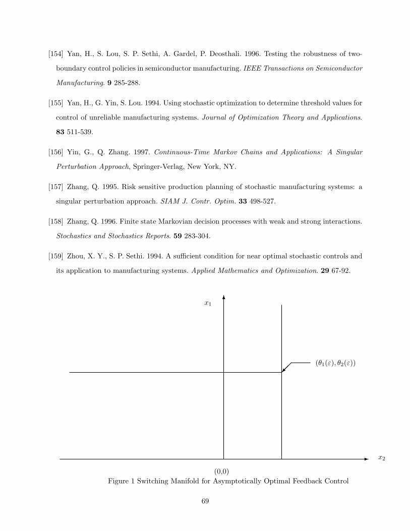
[154] Yan, H., S. Lou, S. P. Sethi, A. Gardel, P. Deosthali. 1996. Testing the robustness of two-
boundary control policies in semiconductor manufacturing. IEEE Transactions on Semiconductor
Manufacturing. 9 285-288.
[155] Yan, H., G. Yin, S. Lou. 1994. Using stochastic optimization to determine threshold values for
control of unreliable manufacturing systems. Journal of Optimization Theory and Applications.
83 511-539.
[156] Yin, G., Q. Zhang. 1997. Continuous-Time Markov Chains and Applications: A Singular
Perturbation Approach, Springer-Verlag, New York, NY.
[157] Zhang, Q. 1995. Risk sensitive production planning of stochastic manufacturing systems: a
singular perturbation approach. SIAM J. Contr. Optim. 33 498-527.
[158] Zhang, Q. 1996. Finite state Markovian decision processes with weak and strong interactions.
Stochastics and Stochastics Reports. 59 283-304.
[159] Zhou, X. Y., S. P. Sethi. 1994. A sufficient condition for near optimal stochastic controls and
its application to manufacturing systems. Applied Mathematics and Optimization. 29 67-92.
-
6
x1
x2
(θ1(ε), θ2(ε))
(0,0)Figure 1 Switching Manifold for Asymptotically Optimal Feedback Control
69
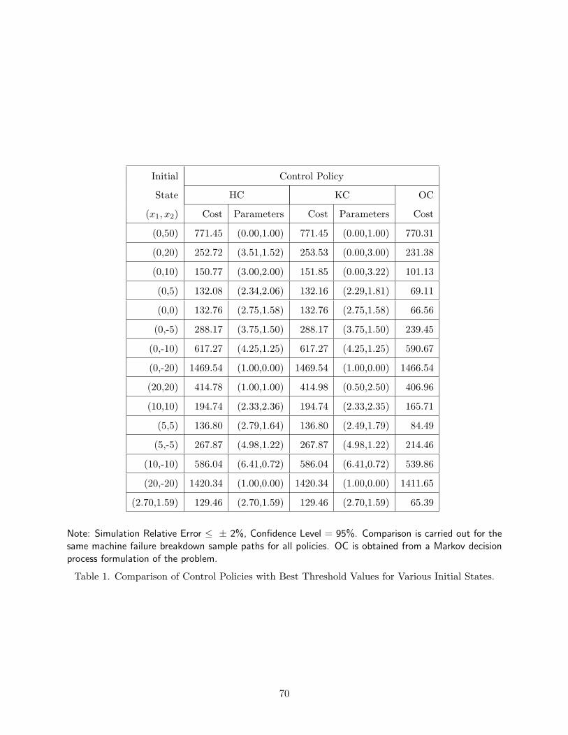
Initial Control Policy
State HC KC OC
(x1, x2) Cost Parameters Cost Parameters Cost
(0,50) 771.45 (0.00,1.00) 771.45 (0.00,1.00) 770.31
(0,20) 252.72 (3.51,1.52) 253.53 (0.00,3.00) 231.38
(0,10) 150.77 (3.00,2.00) 151.85 (0.00,3.22) 101.13
(0,5) 132.08 (2.34,2.06) 132.16 (2.29,1.81) 69.11
(0,0) 132.76 (2.75,1.58) 132.76 (2.75,1.58) 66.56
(0,-5) 288.17 (3.75,1.50) 288.17 (3.75,1.50) 239.45
(0,-10) 617.27 (4.25,1.25) 617.27 (4.25,1.25) 590.67
(0,-20) 1469.54 (1.00,0.00) 1469.54 (1.00,0.00) 1466.54
(20,20) 414.78 (1.00,1.00) 414.98 (0.50,2.50) 406.96
(10,10) 194.74 (2.33,2.36) 194.74 (2.33,2.35) 165.71
(5,5) 136.80 (2.79,1.64) 136.80 (2.49,1.79) 84.49
(5,-5) 267.87 (4.98,1.22) 267.87 (4.98,1.22) 214.46
(10,-10) 586.04 (6.41,0.72) 586.04 (6.41,0.72) 539.86
(20,-20) 1420.34 (1.00,0.00) 1420.34 (1.00,0.00) 1411.65
(2.70,1.59) 129.46 (2.70,1.59) 129.46 (2.70,1.59) 65.39
Note: Simulation Relative Error ≤ ± 2%, Confidence Level = 95%. Comparison is carried out for thesame machine failure breakdown sample paths for all policies. OC is obtained from a Markov decisionprocess formulation of the problem.
Table 1. Comparison of Control Policies with Best Threshold Values for Various Initial States.
70
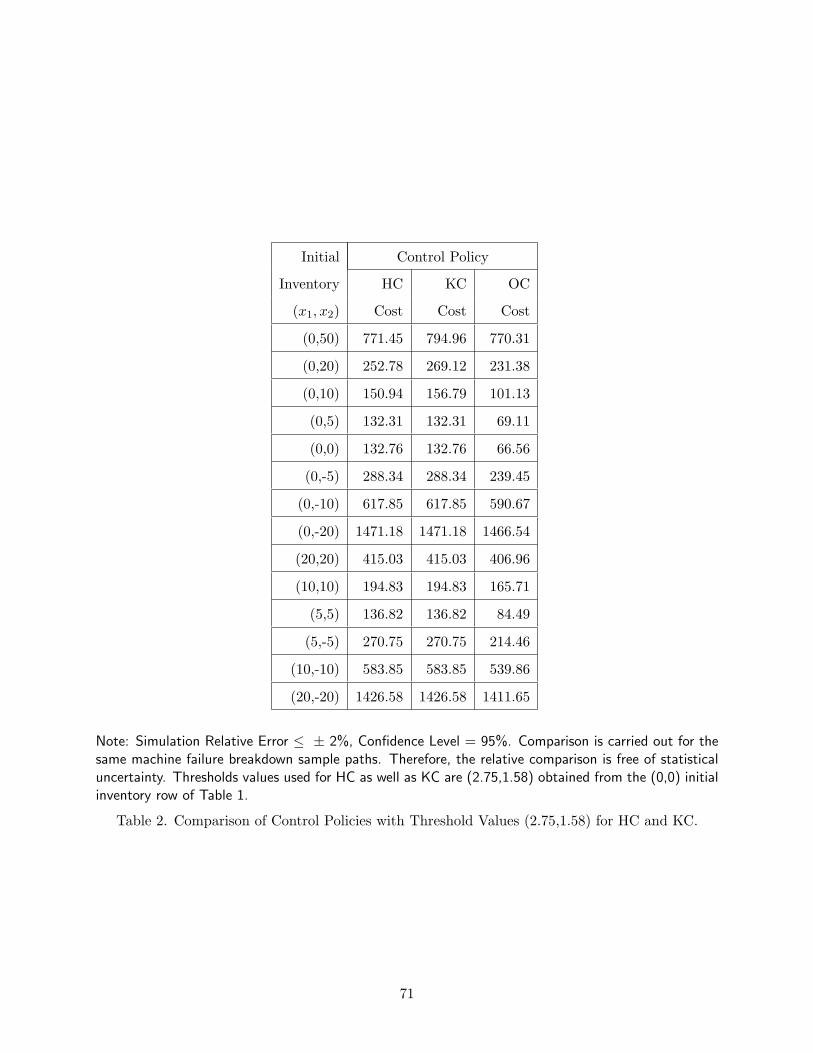
Initial Control Policy
Inventory HC KC OC
(x1, x2) Cost Cost Cost
(0,50) 771.45 794.96 770.31
(0,20) 252.78 269.12 231.38
(0,10) 150.94 156.79 101.13
(0,5) 132.31 132.31 69.11
(0,0) 132.76 132.76 66.56
(0,-5) 288.34 288.34 239.45
(0,-10) 617.85 617.85 590.67
(0,-20) 1471.18 1471.18 1466.54
(20,20) 415.03 415.03 406.96
(10,10) 194.83 194.83 165.71
(5,5) 136.82 136.82 84.49
(5,-5) 270.75 270.75 214.46
(10,-10) 583.85 583.85 539.86
(20,-20) 1426.58 1426.58 1411.65
Note: Simulation Relative Error ≤ ± 2%, Confidence Level = 95%. Comparison is carried out for thesame machine failure breakdown sample paths. Therefore, the relative comparison is free of statisticaluncertainty. Thresholds values used for HC as well as KC are (2.75,1.58) obtained from the (0,0) initialinventory row of Table 1.
Table 2. Comparison of Control Policies with Threshold Values (2.75,1.58) for HC and KC.
71
Related Documents