Optimal actuation in active vibration control using pole ...

Louisiana State UniversityLSU Digital Commons

LSU Doctoral Dissertations Graduate School

2012

Optimal actuation in active vibration control usingpole-placementCarla Ann GuzzardoLouisiana State University and Agricultural and Mechanical College, [email protected]

Follow this and additional works at: https://digitalcommons.lsu.edu/gradschool_dissertations

Part of the Mechanical Engineering Commons

This Dissertation is brought to you for free and open access by the Graduate School at LSU Digital Commons. It has been accepted for inclusion inLSU Doctoral Dissertations by an authorized graduate school editor of LSU Digital Commons. For more information, please [email protected].

Recommended CitationGuzzardo, Carla Ann, "Optimal actuation in active vibration control using pole-placement" (2012). LSU Doctoral Dissertations. 1504.https://digitalcommons.lsu.edu/gradschool_dissertations/1504

OPTIMAL ACTUATION IN ACTIVE VIBRATION

CONTROL USING POLE-PLACEMENT

A Dissertation

Submitted to the Graduate Faculty of the

Louisiana State University and

Agricultural and Mechanical College

in partial fulfillment of the

requirements for the degree of

Doctor of Philosophy

in

The Department of Mechanical Engineering

by

Carla Ann Guzzardo

B.S., Embry-Riddle Aeronautical University

December 2012

ii

ACKNOWLEDGMENTS

Thanks to God for the gifts he has given me and the wonderful universe to play in

with them. Thank you to my parents and family for their unending love and support.

Thanks to Joan, who has walked this road before me and lovingly encouraged me every

step of the way. Thanks to my Sisters for their love, and for helping me to see just how

far courage and persistence can take me. Thanks to my friends inside and out of the

department for their love, encouragement, and excuses to procrastinate.

Special thanks to my co-advisors, Dr. Su-Seng Pang and Dr. Yitshak M. Ram, for

believing in me, even when I did not believe in myself, and for having patience with me.

Thank you to my committee members for their time, input, and consideration.

Thank you to my coworkers and the undergraduates in the Engineering

Communication Studio for giving me a place to call home in Patrick F. Taylor (CEBA)

for the last year, especially Mr. Warren Hull and Mr. David “Boz” Bowles for their

excellent mentoring and friendship, and Ms. Summer Dann and Dr. Warren

Waggenspack for their support.

Finally, thank you to the Louisiana Space Grant Consortium, Dr. Donald W.

Clayton, and the College of Engineering for the monetary assistance to pursue my career

in engineering.

This research is supported by NASA and the Louisiana Board of Regents through

the LaSPACE program (NASA Grant NNG05GH22H and BOR Contract NASA/LEQSF

(2005-10)-LaSPACE) as well as the Louisiana Board of Regents ITRS program under

contract number LEQSF(2007-10)-RD-B-04.

iii

TABLE OF CONTENTS

ACKNOWLEDGMENTS ........................................................................................ ii

LIST OF FIGURES ................................................................................................... v

NOMENCLATURE ................................................................................................. vi

ABSTRACT ........................................................................................................... viii

CHAPTER 1: INTRODUCTION AND LITERATURE REVIEW ......................... 1

1.1 Eigenvalues/Natural Frequencies and Stability ................................................................ 4

1.2 Spillover ............................................................................................................................ 7

1.3 Optimization ..................................................................................................................... 8

1.4 Collocated Sensor/Actuator Pairs ................................................................................... 10

1.5 Technology ..................................................................................................................... 10

1.6 Organization of Thesis .................................................................................................... 11

1.7 Scope and Limitations..................................................................................................... 12

CHAPTER 2: OPEN-LOOP ANALYSIS ............................................................... 13

2.1 Equation of Motion ......................................................................................................... 13

2.2 State Space Analysis ....................................................................................................... 14

2.3 Vibration Response ......................................................................................................... 15

Example 1: Eigenvalues of a Two Degree-of-Freedom System ........................................... 17

CHAPTER 3: POLE PLACEMENT ....................................................................... 20

3.1 Pole Placement ................................................................................................................ 20

3.2 Partial Pole Placement .................................................................................................... 22

Example 2: Partial Pole Placement ....................................................................................... 24

CHAPTER 4: OPTIMIZATION ............................................................................. 27

4.1 Definition of Cost Function ............................................................................................ 27

4.2 Controllability ................................................................................................................. 27

4.2.1 Controllability Matrix ...................................................................................... 28

Example 3: Demonstration of Controllability - State Space Formulation ............................ 29

4.2.2 Vibration Formulation ..................................................................................... 30

Example 4: Demonstration of Controllability - Vibration Formulation ............................... 31

4.3 Statement of Hypothesis ................................................................................................. 32

4.4 Introduction of Equations Used ...................................................................................... 32

4.5 Optimal Actuation in the Single Natural Frequency Modification Problem .................. 33

Example 5: Single Natural Frequency Modification ............................................................ 37

Example 6: Single Natural Frequency Modification with Limited Actuation ...................... 41

Example 7: Checking the Solution on the Physical Domain ................................................ 43

4.6 Optimal Actuation in the Multiple Natural Frequency Modification Problem............... 44

Example 8: Multiple Natural Frequency Modification ......................................................... 46

4.7 Pole Placement by Optimal Actuation ............................................................................ 47

Example 9: Full Eigenvalue Assignment .............................................................................. 49

iv

CHAPTER 5: DEMONSTRATION WITH UNITS ............................................... 52

CHAPTER 6: CONCLUSIONS ............................................................................. 56

REFERENCES ........................................................................................................ 58

APPENDIX A: PROOF OF MINIMUM IN PROBLEM 1 ................................... 61

APPENDIX B: COMPUTER FILES USED IN EXAMPLES .............................. 63

VITA ........................................................................................................................ 75

v

LIST OF FIGURES

Figure 1.1: General matrix block diagram of the state and output equations from D’Azzo

and Houpis (1995, pg. 148). ........................................................................................ 3

Figure 1.2: Graph of complex plane (s-plane) showing response and stability of various

systems by position of eigenvalues, from Franklin et al (1994, pg. 121). .................. 5

Figure 2.1: Simplified model of a two degrees-of-freedom system. ................................ 13

Figure 2.2: Example system with two degrees of freedom. .............................................. 17

Figure 2.3: Simulation of example system displacement (top) and velocity (bottom),

showing high frequency response stabilization from t=0-30 and gradual decrease in

amplitude of vibration for all t. ................................................................................. 19

Figure 3.1: Discrete mass-spring-damper system of two degrees of freedom with applied

control forces. ........................................................................................................... 20

Figure 3.2: Example system with applied control forces. ................................................. 24

Figure 3.3: Simulation of controlled example system displacement and velocity. .......... 26

Figure 4.1: Plot of force selection vector versus optimization criteria, showing lack of

controllability at peak of b1 = -0.807. ........................................................................ 29

Figure 4.2: Two degree-of-freedom controlled system. ................................................... 37

Figure 4.3: The norm of g as a function of 1b . ................................................................ 38

Figure 4.4: Five degree-of-freedom system. ..................................................................... 41

Figure 4.5: The norm of g as a function of 1b . ................................................................ 42

Figure 4.6: The norm of g as a function of 1b , (a) in the complete physical range

11 1 ≤≤− b , (b) zoom on the left minimum, and (c) zoom on the right minimum. .. 47

Figure 4.7: The open-loop system of Example 9. ............................................................. 49

Figure 4.8: Local minimum of η , 2

2

2

13 1 bbb −−= . ........................................................ 50

Figure 4.9: Global minimum of η , 2

2

2

13 1 bbb −−= . ...................................................... 51

Figure 5.1: Control force input needed to control the system when using the optimal force

selection vector. ........................................................................................................ 53

Figure 5.2: Control force input needed to control the system when using the optimal force

selection vector. ........................................................................................................ 54

vi

NOMENCLATURE

a = vector of coefficients

A = system matrix in state-space form

b = force selection vector, also called input vector

C = damping matrix

ie = ith

unit vector

F = net force applied to the system

,f g = velocity and position gain vectors, respectively

I = Identity matrix

K = stiffness matrix

M = mass matrix

m = number of eigenvalues to be assigned

n = system order, degrees-of-freedom

r = number of controllable degrees-of-freedom

S = matrix of open-loop eigenvalues

s = complex Laplace frequency

t = time

u = control input

vii

V = matrix of open-loop eigenvectors

iv = ith

eigenvector

x = state vector

y = control output

1y = vector of controllable eigenvectors

β = input matrix in state-space form (controllability)

Λ = matrix of open-loop eigenvalues

λ = open-loop pole or eigenvalue

µ = closed-loop (assigned) pole or eigenvalue

η = cost function for optimization

ω = open-loop natural frequency

ϑ ,γ , q = partial pole, partial eigenvalue, partial natural frequency placement factors

φ = Lagrangian constraint

Iρ = internal solution

Bρ = boundary solution

ℑ = controllability matrix

τ ,ξ = Lagrange multiplier

w = weighting parameter

viii

ABSTRACT

The purpose of this study was to find and demonstrate a method of optimal

actuation in a mechanical system to control its vibration response. The overall aim is to

develop an active vibration control method with a minimum control effort, allowing the

smallest actuators and lowest control input.

Mechanical systems were approximated by discrete masses connected with

springs and dampers. Both numerical and analytical methods were used to determine the

optimum force selection vector, or input vector, to accomplish the pole placement,

finding the optimal location of actuators and their relative gain so that the control effort is

minimized. The problem was of finding the optimal input vector of unit norm that

minimizes the norm of the control gain vector.

The methods of pole placement and partial pole placement were introduced, and

used to solve various problems, including the active natural frequency modification

problem associated with resonance avoidance in undamped systems, and the single-input-

multiple-output pole assignment problem for second order systems. Both full and limited

controllability were addressed.

During the numerical analysis, it was discovered that the system is uncontrollable

if a control input vector is chosen that is mathematically orthogonal to an eigenvector

associated with a reassigned eigenvalue. Conversely, the optimal input vector was

discovered to be mathematically parallel to an eigenvector. This was proven analytically

through mathematical proofs and demonstrated with various examples. Simulations were

performed in MATLAB and Maple to verify the results numerically.

ix

An example using realistic units was developed to show the order of magnitude

improvement expected by using this method of optimization. All initial conditions and

system parameters were held the same, but the input vector was changed. The optimal

input vector provided an order of magnitude improvement over an evenly distributed

input vector.

The principal conclusion was that by choosing a state feedback input vector that is

mathematically parallel to the eigenvector associated with the open-loop eigenvalue to be

reassigned, or in the case of multiple assignments, in the subspace of the eigenvectors,

the control effort to accomplish pole placement can be reduced to its minimal value.

1

CHAPTER 1: INTRODUCTION AND LITERATURE REVIEW

Vibration is defined by Meirovitch (2001, pg. xvi) as “a subset of dynamics in

which a system subjected to restoring forces swings back and forth about an equilibrium

position.” There are beneficial vibrations, such as in musical instruments to create

sounds or in electrical massage units that offer comfort to tired muscles. However, in

many mechanical systems, vibration can cause damage and shortening of service life.

Constant vibration of a motor can cause fatigue and fracture of supports, earthquake-

induced vibration can damage buildings, and vibration in a spacecraft can jeopardize a

mission.

Free vibration occurs when a system is moved from equilibrium and then

released, with no further input. A system with damping will eventually dissipate energy

and return to equilibrium, while a system without damping will vibrate indefinitely.

Forced vibration occurs when an outside force continually adds energy to the system. If

this energy is not dissipated quickly enough, the vibration will become larger and larger

until a breakdown occurs.

Vibration control is used to eliminate or at least attenuate vibration so that it does

not affect the performance or design life of a mechanical system. Vibration can be

controlled through passive or active means. There is also the possibility of combinations

of passive and active technologies, known as hybrid or semi-active methods as mentioned

by Song (1996).

Passive vibration control consists of parameter modification, including modifying

or adding components by changing the geometry of the system, changing materials for

different elasticity, or adding mass or damping material to the system. This all works to

2

alter the response of the system to outside forces. If these outside, exciting forces are

known in advance, this can be an efficient means of shifting the response of the system so

that vibration does not occur due to those forces.

Resonance is a common problem in undamped or lightly damped systems.

Vibration is subject to superposition, so when the forcing excitation that a system

experiences is close to the natural frequency of the system, the vibration will

constructively interfere and increase in amplitude over time. This can eventually lead to

failure in the system if the amplitude increases beyond design limits. Often, dynamic

absorbers, a type of passive control, are used to alter the response of the system. An

absorber consists of a spring and mass added to the original system and chosen so that the

frequency response of the original system goes to zero at the operating frequency. This

can be a very powerful approach if the problem frequencies are known in advance. Using

a dynamic absorber eliminates resonance at the original frequency, but it creates two

more resonant frequencies around it at different values. In many systems, the excitation

may be unknown or random, meaning that there is still the danger of resonance and

making this type of passive control unsuitable.

Active vibration control can adjust to varying excitation forces as they occur, so

that any vibration is removed from the system. Much work has been done on this topic

and many different methods have been developed, but they all have one unifying trait: the

use of sensors to measure the vibration and actuators to apply forces to the system

components to destructively interfere with the vibration until it is cancelled out. Alkhatib

and Golnaraghi (2003) provides a comprehensive review of active vibration control

topics and methods, including their typical use.

3

All active control methods are implemented by either feedback, feed-forward

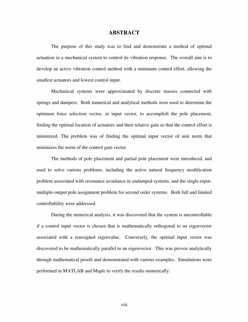
control, or a combination of the two. Figure 1.1 illustrates a general block diagram of a

control system. The input u is on the left. It is altered by various matrices and

computations in the control law, then the output is displayed as y . In feedback control,

as shown by matrix A in Figure 1.1, the state of each degree of freedom is measured and

sent as input to the control system. The control system then calculates the output signal

which is sent to the actuators, so that they can apply the force needed to bring the system

back to equilibrium. Feed-forward control, as shown by matrix D in Figure 1.1, requires

anticipated values of state variables. This can be accomplished in systems where the

excitation forces are known in advance and the response of the system is well understood,

but for a system with random excitation, feedback control is better suited.

Figure 1.1: General matrix block diagram of the state and output equations from D’Azzo

and Houpis (1995, pg. 148).

Feedback control can be implemented in various ways. Single-input, single-

output (SISO) control is used in a single degree-of-freedom system. The state of the

system is measured with sensors and those measurements are sent to the control system

as input. From this input, the output signal is calculated and sent to the actuators. In

multiple-input, multiple-output (MIMO) control, measurements for each degree of

uB ∫

D

A

C+ x&

+

x ++ y

4

freedom are used to generate separate control signals to each actuator and all actuators

work separately. This requires computation of a separate control law for each degree of

freedom. In single-input, multiple-output (SIMO) control, the sensor measurements are

used to generate one control signal that is modified by a separate gain for each actuator.

SIMO has the advantage of working for multiple degrees-of-freedom without needing the

much larger computational power or having the added complexity of a MIMO system.

This thesis investigates the use of SIMO feedback control to accomplish

eigenvalue assignment (also known as pole placement). This is a powerful method of

active vibration control that relies on modifying the response of a system by modifying

its eigenvalues to lie in the left-half of the complex plane, resulting in a stable system that

returns to equilibrium quickly.

1.1 Eigenvalues/Natural Frequencies and Stability

The vibration response of a system can be described by its eigenvalues and

eigenvectors. The eigenvalues may also be called mode frequencies, or poles if the

system is completely controllable and observable. The eigenvectors may also be referred

to as mode shapes.

In a system with damping, the eigenvalues are complex conjugate pairs that

describe the frequency of vibration and the rate at which the vibration decreases or

increases. A system of n degrees-of-freedom will have n complex-conjugate pairs for a

total of n2 eigenvalues. The complex part of each eigenvalue describes the frequency of

the vibration response. A higher magnitude complex part indicates a higher frequency of

vibration. The real part of each eigenvalue describes how quickly the vibration response

5

will decrease or increase. A negative real part indicates that the vibration response will

decrease in amplitude over time, and conversely, a positive real part indicates that the

response will increase in amplitude over time. A higher magnitude real part indicates a

faster increase or decrease.

A system with eigenvalues that all lie in the left-half plane (LHP) of the complex

s-plane, in other words with negative real part, is called a stable system. Stability means

that vibration of all degrees of freedom will decrease over time and the system will

converge to, or at least oscillate about, equilibrium without added control. If any

eigenvalues lie in the right-half plane (RHP), the system is said to be unstable because

one or more degrees of freedom will have increased vibration over time and will require

added control to bring the entire system back to equilibrium. Figure 1.2 shows the

vibration response of systems with eigenvalues in various locations on the complex

plane.

Figure 1.2: Graph of complex plane (s-plane) showing response and stability of various

systems by position of eigenvalues, from Franklin et al (1994, pg. 121).

6

Each eigenvector gives the relative multiplication of displacement between each

degree of freedom for vibration at its associated eigenvalue. A system of n degrees-of-

freedom can have up to 2n eigenvectors and each eigenvector is associated with an

eigenvalue.

In a system with no damping, the eigenvalues are given by the square of the

natural frequencies, as shown in (4). In this case, each eigenvalue can be thought of as a

pair of pure imaginary complex roots,

2( )( )k k k ki iλ ω ω ω= − = , 1, 2,...,k n= . (1)

If no outside forces exist, the system will oscillate about equilibrium indefinitely due to

its conservative nature; there are no dissipative forces to release energy from the system

and allow it to return to equilibrium. It is inherently stable if there is no input of energy

to increase the amplitude of vibration. However, even a very small outside force acting

on the system at or near a natural frequency can cause resonance to occur, where the

amplitude of vibration gradually grows beyond the physical limits of the system. It may

be desirable to shift the natural frequency of the system to prevent resonance. It also may

be desirable to use active control to add damping to the system, so that instead of

oscillating indefinitely, the system will come back to equilibrium.

Many algorithms have been developed to accomplish eigenvalue assignment.

Ackermann’s formula is the classical method, developed in 1972, but it is limited in its

applicability. Miminis and Paige (1988) give an algorithm for pole placement by state

feedback and also review many other pole placement algorithms, each concerned with the

condition number of the resulting gain matrix and the numerical accuracy of the resulting

eigenvalues rather than optimizing the actuation used. Balas (1978) investigates

7

vibration suppression in large space structures by Direct Velocity Feedback, where the

velocity output from sensors is multiplied by a gain in the control system, then applied by

force actuators at the same location. Kimura (1975) shows that eigenvalue assignment by

gain feedback control is possible on systems that are not completely observable.

Mottershead and Ram (2006) offer a good background on full and partial pole

assignment. Datta and Sarkissian (2002) establish the uniqueness and completeness of

solution for the partial eigenvalue assignment problem with single or multiple inputs, and

also discuss controllability.

The classical method of control design involves transforming the equation of

motion of the system to a frequency domain equation. This allows the use of simple

algebraic equations to solve for the gain necessary for pole assignment. However,

transforming the system destroys the symmetry in the second-order nature of the

equations and can lead to computational errors in the final design.

1.2 Spillover

With any active control used, if care is not taken, the system may actually be

made unstable. Any time outside forces, such as from the actuators, are applied, energy

is being added to the system. If applied improperly, the control could result in more

vibration in the system even when less was intended. This can sometimes happen in

partial pole assignment.

In physical cases, there may be a large number of eigenvalues but only a few that

are undesirable. In this case, partial pole assignment can be used to shift these

undesirable eigenvalues to a more favorable position on the complex plane, while

8

ignoring the originally favorable eigenvalues. However, in some instances of partial pole

assignment, the originally favorable eigenvalues may be inadvertently altered and moved

to an unstable position on the complex plane. This is called spillover. In order to avoid

spillover, Datta, Elhay, and Ram (1997) developed a method for partial pole assignment

that does not reduce the model to a first-order transformation first, as is often done in

control design. This allows the second-order nature of the problem to be maintained and

allows a mathematical way of assuring that only the unfavorable eigenvalues chosen by

the designer are reassigned, eliminating spillover.

1.3 Optimization

In most current methods of pole assignment, the input vector, b , is selected by the

designer and the feedback gain vectors, f and g , are unknown. This thesis proposes

solving for optimal actuation, thus lettingb , f , and g be unknown and finding the

combination that allows for the minimal control effort.

In practice, excessive control force from the actuators can lead to damage of the

structure or saturation and improper functioning of the actuators. Optimization can

prevent this. Also by optimizing the actuation for minimal control force, the system

designer can select smaller actuators. In aerospace missions where mass is a strong

system constraint this can be vital to mission success.

Various methods have been researched and used to implement pole assignment

optimally. Optimization in this case refers to effectively applying the control to place the

eigenvalues while minimizing some cost function, typically related to the amount of

control force necessary. Chang and Yu (1996) attempt to have minimal control force to

9

place the eigenvalues, but instead of choosing new values in advance, a technique is used

to find the optimal eigenvalues within a given region which require the minimum control

force to assign, and the gain is found from that. This thesis does not put a limitation on

the eigenvalues, but allows the designer to determine what eigenvalues they would like to

assign and optimizes the gain needed to accomplish that. Gao et al (2003) are concerned

with the placement of actuators in the optimal control of a building with random

parameters. Feedback gain optimization is only done after placement optimization.

Hong, Park, and Park (2006) use H2 and H∞ controls for robustness in the control of a

composite beam with an embedded piezoelectric layer. Jiang and Moore (1996) use least

squares feedback to assign optimal eigenvalues, but the authors admit that this is only a

means of finding a local minimum to the cost function. Karbassi (2001) establishes an

algorithm to minimize the control force during eigenvalue assignment, but uses a

different, more computatively-involved method than is used in this thesis. Lam and Yan

(1997) use robustness, as measured by the spectral condition number, as the cost function

for complete pole placement optimization. Qian and Xu (2005) offer a method of

optimal partial eigenvalue assignment with the condition number of the matrix of

eigenvectors as the cost function, but use an already assigned force selection vector. Ram

and Inman (1999) also offer a method of optimal control while maintaining the second

order nature of the vibration equations, instead of relying on first-order realization. An

optimization solution with a cost function weighted on both control force and response of

the system is offered, but it does not use the same method of pole assignment as this

thesis.

10

1.4 Collocated Sensor/Actuator Pairs

Both Schulz and Heimbold (1983) and Yang and Lee (1993) study the

optimization of feedback control on a system with non-collocated sensors and actuators.

This non-collocation can lead to an unstable system if not implemented properly.

However, Dosch, Inman, and Garcia (1992) show that a collocated sensor/actuator pair is

possible with a self-sensing piezoelectric actuator; therefore, the assumption of collocated

sensor/actuator pairs is used in this thesis.

1.5 Technology

Vasques and Rodrigues (2006) compare various control schemes, both classical

and modern, and show the response of a piezo-electrically controlled beam to those

controls. It shows that application of the technology is possible at this time, though work

is needed to implement it on a large scale. Matsuzaki, Ikeda, and Boller (2005) introduce

a new Smart Metal Alloy which is partially magnetized and actuated by electromagnetic

field excitation. This is the sort of material needed for devices that are fast enough to

perform pole placement on a large scale in structural systems. The material was not

available at the time of publication, so numerical results are given in place of lab

experimentation results. Zhang et al (2004) also present a future actuator material that

could be used for active vibration control. An experimental setup is presented and results

show good response by the closed-loop system, again showing that the technology exists

to implement this type of control.

11

1.6 Organization of Thesis

The thesis is organized as follows. Chapter 2 introduces the mathematical

formulae necessary to discuss vibration of an open-loop system, both with and without

damping. The equation of motion is developed and state space analysis is used to

determine the eigenvalues and eigenvectors of a system. The vibration response is found

from initial conditions. An example problem is offered to demonstrate.

Chapter 3 continues with the development of a vibration control method using

single-input-multiple-output feedback control. The formula for partial pole assignment

developed by Datta, Ram, and Elhay (1997) is introduced. The system of the first

example is now used in an example of this pole placement technique to increase stability.

Chapter 4 uses the results of Chapters 2 and 3 to develop an optimization method,

through variation of the input vector and gain vectors, to minimize control effort as

defined by a cost function. Observations on the controllability of the system and a theory

developed from this observation are extended through various examples. The work of

much of Chapter 4 is to be published in a future issue of Mechanical Systems and Signal

Processing and is presented here with permission.

Chapter 5 introduces units to the equations and solves Example 9 again to find the

magnitude of control force used in actuation of the system, both optimal and arbitrary.

Chapter 6 involves a brief discussion of the results of Chapter 5 and draws

conclusions on the effectiveness of the theory.

12

Finally, the Appendices provide additional resources, including a proof of the

solution of Problem 1 from Chapter 4 being the minimum on the domain, and all

computer files used to generate the solutions seen in the thesis.

1.7 Scope and Limitations

This thesis serves as an initial investigation into the topic of optimal actuation.

Very general and simplified linear models and examples are used to demonstrate the

theory and to verify the mathematical proofs. Only feedback control is used to

implement pole placement and partial pole placement.

Due to the constraints of time and equipment, no physical experimentation has

been done, only computer simulations. There is no consideration in this work for non-

linear systems or systems where time delay in the controls is a factor. There is also no

statement made to what value eigenvalues should be assigned, and no control of

eigenvectors. Those decisions are left up to the reader.

13

CHAPTER 2: OPEN-LOOP ANALYSIS

2.1 Equation of Motion

A mechanical system can be modeled as a simplified combination of lumped

masses joined by springs and dampers. The masses model the inertia of the system; the

springs model the resistance to motion or stiffness of the system; and the dampers model

the energy dissipation of the system. Each mass-spring-damper combination represents

one degree of freedom of the physical system. A two degrees-of-freedom system is

modeled in Figure 2.1.

x1 x2

k1 k2

c1 c2

m1 m2

x1 x2

k1 k2

c1 c2

m1 m2

k1 k2

c1 c2

m1 m2

Figure 2.1: Simplified model of a two degrees-of-freedom system.

Each block has mass m ; each spring has a coefficient of stiffness k ; and each

damper has a coefficient of damping c . The position of each block from equilibrium is

measured as x . Each block is constrained to move only in the x direction.

The equation of motion of a system with n degrees-of-freedom is derived from

Newton’s second law of motion. If there are no outside forces on the system, the

summation of forces on the thi block is

0=++=∑ iiiiiii xkxcxmF &&& (2)

The equation of motion of the entire system is represented in matrix form as

0KxxCxM =++ &&& (3)

14

where M , C , K are n x n real matrices. Dots denote derivatives with respect to time.

Separation of variables is used to find a solution for Equation (3). This allows

identification of the eigenvalues and eigenvectors of the system.

Consider a solution of the form

ste=x v (4)

and substitute into Equation (3). The equation of motion becomes

2 st st sts e s e e+ + =Mv Cv Kv 0 (5)

The exponential function is nonzero for all positive values of time t ; therefore it

can be cancelled out of the equation. The quadratic eigenvalue problem remains.

( )2s s+ + =M C K v 0 . (6)

The solution =v 0exists for all values of s. This trivial solution, when =x 0 for

all time, does not tell us anything about the vibration response of the system, so we

concentrate only on solutions where ≠v 0 , or when

2 0s s+ + =M C K . (7)

The determinant equation is a polynomial of order n2 with roots is , 1, 2,..., 2i n= .

Each root is is an eigenvalue of the system. Once the eigenvalues are known, each

eigenvector iv is found by solving Equation (6), where is is the associated eigenvalue.

2.2 State Space Analysis

Two state space variables are defined for the system in Figure 2.1. Both

position x and velocity x& are vectors of n length. The state space equations of motion are

15

= −

I 0 x 0 I x

C M x K 0 x

&

&& &. (8)

By defining

=

x

xz

&,

−=

0K

I0A , and

=

MC

0IB , (9)

and rearranging, Equation (8) becomes

0zBAz =− & . (10)

Try a solution of the form

( ) stt e=z U (11)

where U is the constant vector

1 2 2

1 1 2 2 2 2

n

n ns s s

=

v v vU

v v v

L

L. (12)

This results in the problem

st ste s e− =AU BU 0 (13)

which can be simplified to the generalized eigenvalue problem,

( )s− =A B U 0 . (14)

Equation (14) can be easily solved for the eigenvalues and eigenvectors of the

system using an off-the-shelf commercial software program such as MATLAB.

2.3 Vibration Response

The output of the system is the position and velocity of each degree-of-freedom,

( )t

=

xy

x&, (15)

assuming all degrees-of-freedom to be observable.

16

The general solution of position for each degree of freedom is the linear

combination of the n2 solutions for each eigenvalue and eigenvector pair, from Equation

(4),

2

1

i

ns t

i i

i

a e=

=∑x v , (16)

where ia are constant coefficients determined by initial conditions of the system.

Similarly, the solution of velocity is the time derivative of Equation (16),

2

1

i

ns t

i i i

i

a s e=

=∑x v& . (17)

To impose initial conditions, solve Equations (16) and (17) at time 0t = . This

gives initial position

2

1

(0)n

i i

i

a=

=∑x v , (18)

and initial velocity

2

1

(0)n

i i i

i

a s=

=∑x v& . (19)

In matrix form, this is written

0

0

=

xUa

x& (20)

where, U is from Equation (12) and ( )T

naaa 221 L=a . To determine the

coefficients ia in Equation (20), U must be invertible.

Once the eigenpairs ( ), , 1,2,..., 2i is i n=v and coefficients ia are known, the value of

( )ty is known from Equations (15)-(17).

17

Example 1: Eigenvalues of a Two Degree-of-Freedom System

Consider a simple uncontrolled, vibrating system of two degrees of freedom, as

shown in Figure 2.2.

x1 x2

5 10

0.2

1 2

x1 x2

5 10

0.2

1 2

Figure 2.2: Example system with two degrees of freedom.

The system can be modeled as in Equation (3), with equation of motion

1 1 1

2 2 2

1 0 0.2 0.2 15 10 0

0 2 0.2 0.2 10 10 0

x x x

x x x

− − + + = − −

&& &

&& &. (21)

State space analysis leads to Equation (10) as

1 1

2 2

1 1

2 2

0 0 1 0 1 0 0 0 0

0 0 0 1 0 1 0 0 0

15 10 0 0 0.2 0.2 1 0 0

10 10 0 0 0.2 0.2 0 2 0

x x

x x

x x

x x

− =

− − − −

&

&

& &&

& &&

. (22)

Solving the generalized eigenvalue problem of Equation (14) using MATLAB,

the eigenvalues and eigenvectors of the system in Figure 2.2 are found to be

-0.1472 - 4.3170i 0 0 0

0 -0.1472 + 4.3170i 0 0

0 0 -0.0028 - 1.1575i 0

0 0 0 -0.0028 + 1.1575i

=

S , (23)

0.0263 - 0.1995i 0.0263 + 0.1995i 0.0082 - 0.6269i 0.0082 + 0.6269i

-0.0114 + 0.0728i -0.0114 - 0.0728i 0.0055 - 0.8563i 0.0055 + 0.8563i

0.8573 + 0.1427i 0.8573 - 0.1427i 0.7257 + 0.0113i 0.7257 - 0.0113i

-0.3

=U

127 - 0.0601i -0.3127 + 0.0601i 0.9912 + 0.0088i 0.9912 - 0.0088i

. (24)

18

The first two rows of the matrix U are the eigenvectors of the system, also known as

matrix v . Note there are 2 4n = eigenvalues and eigenvectors, 2n = pairs of complex

conjugates.

Also note that the eigenvalues of the system all have negative real part, therefore

the system is stable.

Assume a given initial position and velocity of

0

1

0

=

x , 0

0

1

=

x& . (25)

The coefficients for Equation (16) are

0.0025 + 1.9711i

0.0025 - 1.9711i

0.3872 + 0.1652i

0.3872 - 0.1652i

=

a . (26)

The output y can be found as a function of time following Equations (15)-(17)

and using the calculated values. A simulation of this example system is shown in Figure

2.3. Each figure shows the high and low frequency modes in the initial response of

position and velocity. The high frequency response stabilizes more quickly than the low

frequency, due to the eigenvalue being further in the left-half plane on the complex plane.

The lower frequency response gradually decreases amplitude over time.

This example shows that the system is indeed stable and will converge to

equilibrium; however, that convergence may take much longer than desired. There may

be constraints on the performance characteristics of the design to minimize vibration or to

more quickly damp out such oscillations to below a threshold of amplitude.

19

Figure 2.3: Simulation of example system displacement (top) and velocity

(bottom), showing high frequency response stabilization from t=0-30 and

gradual decrease in amplitude of vibration for all t.

20

CHAPTER 3: POLE PLACEMENT

3.1 Pole Placement

Pole placement or pole assignment, also called eigenvalue assignment in various

papers, involves reassigning the eigenvalues of the system to reduce its dynamic

response. This can include moving eigenvalues to the LHP for stability, or moving

further to the left if they are already stable, to reduce the time to convergence at

equilibrium. This assignment is achieved through active damping and active stiffness,

modifying the damping and stiffness of the closed loop system through applied forces.

A control force ( )u tb is applied to the system, as in Figure 3.1. The control

input, ( )u t , includes the velocity and position gain vectors, f and g , where

( ) T Tu t = +f x g x& . (27)

This results in a new equation of motion,

( )u t+ + =Mx Cx Kx b&& & (28)

b1u(t) b2u(t)

x1 x2

k1 k2

c1 c2

m1 m2

b1u(t) b2u(t)

x1 x2

k1 k2

c1 c2

m1 m2

x1 x2

k1 k2

c1 c2

m1 m2

k1 k2

c1 c2

m1 m2

Figure 3.1: Discrete mass-spring-damper system of two degrees of freedom with applied

control forces.

Only those eigenvalues which lie outside of the performance constraints in the

design require reassignment. The force selection vector, b , determines on which masses

the control input is applied and with what gain, where

21

( )1 2

T

mb b b=b K . (29)

This is an example of single-input, multiple output (SIMO) control. The only

input is fromu , but the force selection vector applies this input to multiple degrees-of-

freedom, resulting in multiple outputs.

MATLAB’s place command can be used to assign all new eigenvalues to the

system. Begin by assigning a matrix

1 1− −

= −

0 IA

M K M C. (30)

The command gf=place(A,-[zeros(n,1);inv(M)*b],s)assigns the

vector

=

ggf

f, (31)

which contains both position and velocity gain vectors necessary to reassign the system

eigenvalues to the set s .

There is a related problem associated with the avoidance of resonance and near

resonance phenomena in harmonically excited undamped systems. In this problem it is

desired to shift a few natural frequencies from the spectral neighborhood of the exciting

forces. There is a wealth of literature associated with this problem where the spectral

modification is achieved by passive means, i.e., by physical structural modification

altering the rigidity and density of the system, see e.g., Elishakoff (2000), Lawther

(2007), McMillan and Keane (1996), Mottershead and Ram (2006), Ram (1994), and

Ram and Blech (1991). Here we address the associated problem where the spectral

modification is done by active vibration control implemented by state feedback. The

22

problem may be regarded as a reduced form of the pole placement problem where 0C =

and 0f = . We name this problem the active natural frequency modification problem.

3.2 Partial Pole Placement

In full pole placement, all modes of the open loop system are reassigned to new

eigenvalues. In practice, this can be an impossible and unnecessary task. A flexible

structure may have a very large number of modes, but only a selection of those may be

unstable or outside of performance requirements. Higher frequency modes will typically

damp out much faster than low frequency modes. It is necessary only to reassign those

modes which will cause problems in operation. Partial pole placement reassigns only

those eigenvalues chosen while leaving all other open loop eigenvalues unchanged.

The original set of open loop eigenvalues, Λ, consists of those to be replaced and

the remaining eigenvalues,

1

2

Λ Λ = Λ

, (32)

where

1

1

m

λ

λ

Λ =

O (33)

is the set to be replaced.

Similarly, the open-loop eigenvectors consist of those to be replaced and those

remaining unchanged,

[ ]1 2|=V V V , (34)

where

23

[ ]1 1 2, ,..., m=V v v v (35)

is the set to be replaced.

If the number of reassigned eigenvalues is m , then the new eigenvalues of the

system will be assigned to the set { }1 2, ,..., mµ µ µ and the remaining unchanged

eigenvalues will be assigned to the set { }1 2 2, ,...m m ns s s+ + .

The velocity gain vector is chosen as

1 1f = MVΛ q (36)

and the position gain vector is chosen as

1g = -KV q (37)

where

1

1, 1,2,...,

mj j i j

j Tij j i ji j

s sj m

s s s

µ µ

=≠

− −= =

−∏q

b v (38)

The result is a modified eigenvalue matrix with the new assigned eigenvalues but

retaining the initial eigenvalues not meant to be changed, as shown in Datta, Elhay, and

Ram (1997).

Once the force control vectors are known, the equation of motion can be solved

for the new eigenvectors by including the control forces, giving the equation

( )T T+ + = +Mx Cx Kx b f x g x&& & & . (39)

This can be solved by grouping terms of x and solving by separation of variables,

as in the previous section.

( ) ( )2 T Ts s + − + − = M C bf K bg v 0 (40)

The state space equation of motion, similar to Equation (8), becomes

24

( ) ( )T T

= − − −

I 0 0 Ix x

C bf M K bg 0x x

&

&& &. (41)

Following the procedure of Equations (9)-(14), the eigenvectors of the new

eigenvalues can be found. The response of the system can also be found by following the

procedure of Equations (15)-(20).

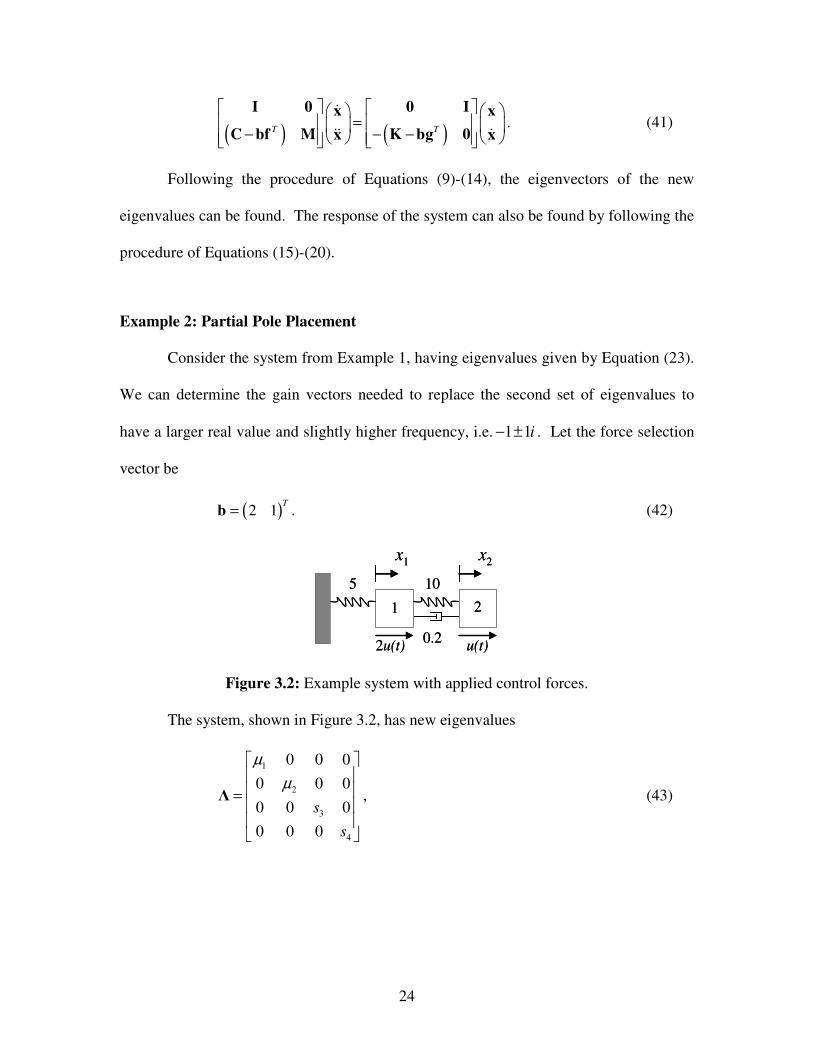
Example 2: Partial Pole Placement

Consider the system from Example 1, having eigenvalues given by Equation (23).

We can determine the gain vectors needed to replace the second set of eigenvalues to

have a larger real value and slightly higher frequency, i.e. 1 1i− ± . Let the force selection

vector be

( )2 1T

=b . (42)

2u(t) u(t)

x1 x2

5 10

0.2

1 2

2u(t) u(t)

x1 x2

5 10

0.2

1 2

Figure 3.2: Example system with applied control forces.

The system, shown in Figure 3.2, has new eigenvalues

1

2

3

4

0 0 0

0 0 0

0 0 0

0 0 0

s

s

µ

µ

=

Λ , (43)

25

-1 - 1i 0 0 0

0 -1 + 1i 0 0

0 0 -0.1472 + 4.3170i 0

0 0 0 -0.1472 - 4.3170i

=

Λ . (44)

Using the procedure from Datta, Elhay, and Ram (1997),

1 1 2 11

1 1 2 1

2 2 1 22

2 2 1 2

1

1

T

T

s s

s s s

s s

s s s

µ µ

µ µ

− −=

−

− −=

−

qb v

qb v

. (45)

This leads to position gain vector

0.5930

1.6168

− =

− f (46)

and velocity gain vector

0.1478

0.5771

− =

− g . (47)

These are the gain vectors necessary to move only the undesired eigenvalues to a new

value while retaining the other eigenvalues of the system.

The response of the closed loop system is shown in Figures 3.3 and 3.4. Note that

the response decreases in amplitude much more quickly than that of the open loop

system, shown in Figures 2.3 and 2.4. By 30t = , the amplitude of vibration has

decreased two orders of magnitude.

Note that this example is limited by the choice of force selection vector, b . The

value chosen does not allow assigning the eigenvalue to any higher frequencies using this

method. If the attempt is made, a solution cannot be found that correctly assigns the

eigenvalues. The resulting performance is that of an unstable system.

26

Figure 3.3: Simulation of controlled example system displacement and velocity.

27

CHAPTER 4: OPTIMIZATION

4.1 Definition of Cost Function

The choice of force selection vector, b , affects the values of the position and

velocity gain vectors, f and g . These values, in turn, determine how much control force

must be exerted by the actuators in the physical system. Minimizing the control force

allows use of the smallest possible actuators and the minimum applied voltage during

actuation.

We leave the definition of control force up to the designer of the system and show

that any definition can be achieved through this method. We will use the cost function

2 2

wη = +f g (48)

to demonstrate the method.

In addition, the force selection vector is constrained to

1=b . (49)

Without this constraint, the force selection vector could theoretically be made very large

to allow the position and velocity gain vectors to be very small, with the same control

effect. However, physically this would not minimize the actuation needed.

4.2 Controllability

A system is said to be completely controllable if each output state is constrained

by the input control vector [D’Azzo]. To determine if this is true, a controllability matrix

can be assembled from the state equations of the system. The optimization criterion

28

decided upon in Section 4.1 can also show where the system becomes uncontrollable.

There is a peak in the graph of optimization criterion versus force selection vector, shown

in Figure 4.1, which represents the choice of force selection control vector that is not able

to control the given system of Example 2. This is demonstrated through both state space

formulation and vibration formulation.

4.2.1 Controllability Matrix

Using the equation of motion of the closed-loop system (28), the state-space

formulation is

( )tuβAzz +=& , (50)

where

=

x

xz

&,

−−=

−− CMKM

I0A

11,

=

− bM

0β

1, (51)

( ) zφTtu = , and

=

f

gφ . (52)

The controllability matrix is defined as

2 1n− ℑ = β Aβ A βL . (53)

The system is only controllable if the controllability matrix has full rank, when

rank( ) 2nℑ = . (54)

Otherwise, it is uncontrollable. In the case where 1n×= ℜb , the system is uncontrollable

if det( ) 0ℑ = .

29

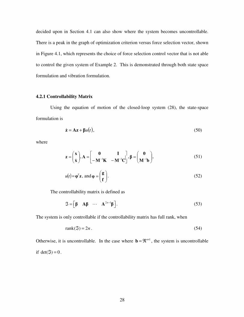
Example 3: Demonstration of Controllability - State Space Formulation

Graphical evidence of controllability can be shown by repeating Example 2 and

analyzing a plot of force selection vector versus the optimization criterion, as in Figure

4.1. To create the graph, the first component of the force selection vector is varied from

-1 to 1 with a step size of 0.001. The force selection vector is constrained to having a

norm of 1, so the second element is calculated as

2

2 11b b= − , (55)

and the force selection vector is

1

2

b

b

=

b . (56)

Figure 4.1: Plot of force selection vector versus optimization criteria, showing lack of

controllability at peak of b1 = -0.807.

The graph peaks when the first element of the force selection vector is -0.806.

The resulting value of the second element is 0.592, therefore

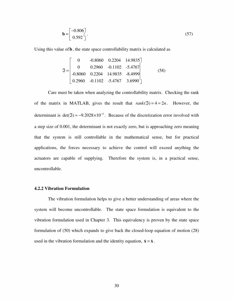
30

0.806

0.592

− =

b . (57)

Using this value of b , the state space controllability matrix is calculated as

0 -0.8060 0.2204 14.9835

0 0.2960 -0.1102 -5.4767

-0.8060 0.2204 14.9835 -8.4999

0.2960 -0.1102 -5.4767 3.6990

ℑ =

(58)

Care must be taken when analyzing the controllability matrix. Checking the rank

of the matrix in MATLAB, gives the result that ( ) 4 2rank nℑ = = . However, the

determinant is 4det( ) 9.2028 10−ℑ = − × . Because of the discretization error involved with

a step size of 0.001, the determinant is not exactly zero, but is approaching zero meaning

that the system is still controllable in the mathematical sense, but for practical

applications, the forces necessary to achieve the control will exceed anything the

actuators are capable of supplying. Therefore the system is, in a practical sense,

uncontrollable.

4.2.2 Vibration Formulation

The vibration formulation helps to give a better understanding of areas where the

system will become uncontrollable. The state space formulation is equivalent to the

vibration formulation used in Chapter 3. This equivalency is proven by the state space

formulation of (50) which expands to give back the closed-loop equation of motion (28)

used in the vibration formulation and the identity equation, =x x& & .

31

From (38), we see that the control forces f and g require the calculation of

1

, 1, 2,...,T

j

j m=b v

. (59)

wherejv are those eigenvectors associated with eigenvalues to be reassigned.

If the force selection vector,

b , is orthogonal to any of these eigenvectors of the

open-loop system, this calculation results in a division by zero. This would require an

infinite control force to completely control the system using that force selection vector.

Physically this is impossible, making the system uncontrollable for chosen force selection

vectors that are orthogonal to any eigenvector associated with a reassigned eigenvalue of

the open-loop system.

Example 4: Demonstration of Controllability - Vibration Formulation

Using the vibration formulation, the system is analyzed for the same force

selection vector, b , as in Example 3. This vector,b , is checked for orthogonality with the

open-loop eigenvectors,

j

v , 1,2,..., 2j n= . Orthogonality is proven if

0T

j =b v . (60)

Since each eigenvector is part of a complex conjugate pair, only one of each pair needs to

be checked.

For this example,

[ ]1

0.0133 0.22560.806 0.592 0.0124 0.2308

0.0028 0.0827

Ti

ii

− − = − = + +

b v , (61)

[ ]1

0.0040 0.62590.806 0.592 0.0034 0.0015

0.0112 0.8548

Ti

ii

− − = − = − − +

b v . (62)

32

Again, discretization errors keep (62) from equaling zero exactly, but the value

approaches zero. Thus, the force selection vector of (57) is very close to orthogonal to

the eigenvector 3v . By the vibration formulation, the system is not controllable at this

force selection vector.

4.3 Statement of Hypothesis

This uncontrollability associated with a mutually orthogonal eigenvector and

force selection vector leads to the hypothesis that, conversely, the optimal force selection

vector exists parallel to the reassigned eigenvector. In the case where multiple

eigenvectors exist, the optimal force selection vector exists in the subspace of those

eigenvectors. This hypothesis is proven mathematically in a journal article, written with

co-authors Su-Seng Pang and Yitshak M. Ram, accepted for publication in Mechanical

Systems and Signal Processing, the body of which is reprinted by permission in sections

4.4 through 4.7.

4.4 Introduction of Equations Used

We use the notation

T

nxxx

∂

∂

∂

∂

∂

∂=

∂

∂ γγγγL

21x (63)

to define the partial derivatives of a scalar function ( )xγ with respect to the elements of

x . We also use the following basic relations,

Axx

Axx2=

∂

∂ T

, (64)

which holds for any constant symmetric matrix A , and

33

ax

xa=

∂

∂ T

, (65)

which holds for any constant vector a . By norm we mean the Euclidian norm.

4.5 Optimal Actuation in the Single Natural Frequency Modification

Problem

The equations of motion for an open-loop undamped system are a simplified

version of those presented in Chapter 2 for a full system, and can be modeled as

0KxxM =+&& . (66)

The solution to (66) takes the form

( ) tt ωsinvx = (67)

where v is a constant vector. Substituting (67) in (66) gives the generalized eigenvalue

problem

( ) 0vMK =− λ , 2ωλ = , (68)

where { }n

kk 1=λ and { }n

kk 1=v are the eigenvalues and eigenvectors of the open-loop system.

In the natural frequency assignment problem, where the eigenvalues of (68) are assigned

to be real, the closed-loop system (27)-(28) is reduced to

( )tubKxxM =+&& , (69)

where

( ) xgTtu = . (70)

This leads to the eigenvalue problem

( ) 0wMbgK =−− µT , (71)

34

where { }n

kk 1=µ and { }n

kk 1=w are the eigenvalues and eigenvectors of the closed-loop

system. In the partial natural frequency assignment problem we wish to change by the

control some m eigenvalues, nm < , of the open-loop system { }m

kk 1=λ to a given real set

{ }m

kk 1=µ while keeping the rest of the eigenvalues unchanged.

Note that control here is accomplished only through induced stiffness, in other

words, only by using the position gain vector g. Although adding induced damping by

using a velocity gain vector f may help control the system more efficiently, it is easier to

introduce the concepts and proofs by using this simpler form of only one gain vector.

Section 4.7 uses both gain vectors to find the solution. The procedure does not change,

however the Lagrange multiplier complexity and number of equations increases with use

of both gain vectors.

Lemma 1

With

∑=

=m

k

kk

1

Mvg ϑ (72)

where

∏≠= −

−−=

m

kii ik

ik

k

T

kkk

1 λλ

µλµλϑ

vb, (73)

the eigenvalues of (71) are

{ } { }nmmk λλµµµ LL 11 += . (74)

The lemma is a straightforward reduction of Theorem 3.2 in Datta, Elhay and Ram [2].

35

Consider the partial natural frequency assignment problem where 1=m . That is

an undamped system where only one natural frequency is to be reassigned. The problem

of optimal actuation in this case may be formulated as follows:

Problem 1

Given: M , K , 1µ

Find: b , and g such that

{ } { }n

n

kk λλµµ L211=

= (75)

and where Tbg attains its minimum.

Solution

The solution is

1

1

v

vb = , 1Mvg γ= (76)

where

1

11

v

µλγ

−= (77)

Proof (partial):

We first note that by physical reasoning Problem 1 has a minimal norm solution.

The solution is either internal to the domain of the physical parameters, ℜ∈kb , or on the

boundary of the domain, where for some, but not all, 0=kb .

Let b and g be one solution of Problem 1. Then bβ and g1−β is another

solution for any real scalar 0≠β . Hence, without loss of generality, we may look for a

36

solution where 1=b . This prerequisite is satisfied by the first equation in (76). Since

gbbg =T , the solution to Problem 1 is obtained by minimizing ggT subject to 1=bbT .

By Lemma 1

1

1

11 Mvvb

gT

µλ −= , (78)

hence if there exists a local minimum within the domain it could be located by finding the

stationary values of the Lagrangian

( ) ( )( )

bbvMvvb

b TT

TL ξ

µλ+

−= 1

2

12

1

2

11 , (79)

where ξ is a Lagrange multiplier imposing the unit norm constraint on b . Differentiating

(79) with respect to b gives

( )( )

0bvvb

vbvMv

b=+−−=

∂

∂ξµλ 22 14

1

11

2

1

2

11 T

TTL

. (80)

Note that Equation (80) has a unique solution, up to a sign change,

( ) ( )13

1

1

2

1

2

11 vv

vMvb

ξ

µλ T−= , (81)

and

( ) ( )11

1

2

1

2

11

vv

vMvT

Tµλξ

−= . (82)

It is shown in Appendix A that this solution is a local minimum.

To show that the internal solution is in fact the global minimum we need to prove

that Tbg of the internal solution is smaller than the minimal norm solution on the

boundary of the domain. A formal proof is given at the end of this section.

37

Meanwhile we would be satisfied with the heuristic argument that the minimal

norm solution on the boundary of the domain is equivalent to the optimal solution where

some degrees of freedom are not subject to actuation. Such a system is less flexible to

control and requires larger control effort.

Example 5: Single Natural Frequency Modification

Consider the two-degree-of-freedom system shown in Figure 4.2, where 1=k

and 1=m . The mass and stiffness matrices of the open-loop system are

=

10

01M ,

−

−=

11

12K .

The eigenvalues and normalized eigenvectors of (68) are

==

8507.0

5257.03820.0 11 vλ ,

−==

5257.0

8507.06180.2 22 vλ .

m

k k

m

( )tub1 ( )tub2

1x 2x

m

k k

m

( )tub1 ( )tub2

1x1x 2x2x

Figure 4.2: Two degree-of-freedom controlled system.

We wish to find the input vector ( )Tbb 21=b , where 12

2

2

1 =+ bb , and the

minimal norm vector g such that the eigenvalues kµ of the closed-loop system (71),

discarding the damping term, are

2.61802 221 === λµµ .

We have changed the parameter 1b in the range 11 1 ≤≤− b and evaluated g that

assigns the eigenvalues of the closed-loop system as required. The graph of g as a

38

function of 1b is shown in Figure 4.3a. The singularity at 8507.01 −=b corresponds to

the maximal control effort where b is orthogonal to 1v and the system is not controllable

as shown in section 4.2.

g

1b 1b

(a) (b)

2

12 1 bb −= 2

12 1 bb −=

g

1b 1b

(a) (b)

2

12 1 bb −= 2

12 1 bb −=

Figure 4.3: The norm of g as a function of 1b .

Figure 4.3b zooms on the graph in the interval 10 1 ≤≤ b . It shows that the

minimum of g attains at 5257.01 =b , with corresponding 8507.02 =b , where as

predicted by (76) 1vb = since 1=b .

Generally the eigenvector 1v is fully populated and hence the optimal input vector

b that solves Problem 1 should be fully populated as well. This implies that in physical

applications there is an actuator at each degree of freedom to realize the control. However

some degrees of freedom in a realistic system are usually not accessible to actuation and

therefore the number of actuators r is smaller than the number of degrees of freedom,

nr < . We therefore define below the problem of finding the optimal input vector for the

case where some specified elements in b vanish by design. Since the degrees of freedom

are numbered arbitrarily, without loss of generality, we may number the degrees of

freedom in such a way that

39

=

0

bb

1, (83)

where rℜ∈1b . The related optimal assignment of one eigenvalue in this case is

formulated as follows.

Problem 2

Given: M , K , 1µ , and an integer r , nr < .

Find: b , and g such that

{ } { }n

n

kk λλµµ L211=

= (84)

subject to the constraints

0=beT

k, nrrk ,...,2,1 ++= (85)

where ke is the thk unit vector and where Tbg attains its minimum.

Solution:

Denote

=

2

1

1y

yv rℜ∈1y (86)

Then

=

0

y

yb

1

1

1 (87)

Proof:

We wish to minimize

1

2

1

2

1 vMvgg TT ϑ= (88)

subject to

1=bbT (89)

40

and

0=beT

k, nrrk ,...,2,1 ++= . (90)

Define the Lagrangian

( ) bEτbbvMvb TTTTL ++= ξϑ 1

2

1

2

1 (91)

where

[ ]nrr eeeE L21 ++= (92)

and ξ and kτ are Lagrange multipliers. Differentiating

( )( )

0Eτbvvb

vbvMv

b=++−−=

∂

∂ξµλ 2

214

1

11

2

1

2

11 T

TTL

(93)

gives

( )( )

Eτbvvb

vMv=−

−ξ

µλ2

213

1

1

2

1

2

11

T

T

. (94)

We will now show that with b given by (87) there exist ξ and τ such that the

equations in (94) are all satisfied.

Substituting (87) in (94) gives for the first r equations

( )

( )0y

yy

yy

vMv=−

−1

1

15.1

11

1

2

1

2

11 ξµλT

T

(95)

Hence with

( )

11

1

2

1

2

11

yy

vMvT

Tµλξ

−= (96)

the equations in (95) are satisfied. The other rn − equations of (94) are obviously

satisfied when the vector of Lagrange multipliers τ is chosen as

41

( )

( ) 23

1

1

2

1

2

112y

vb

vMvτ

T

Tµλ −= . (97)

Similar to the proof in Appendix A it could be shown that this solution is a local

minimum. We note that by (87) we have 1=b and hence

TT bggg = (98)

i.e., by minimizing ggT the minimum of Tbg is attained.

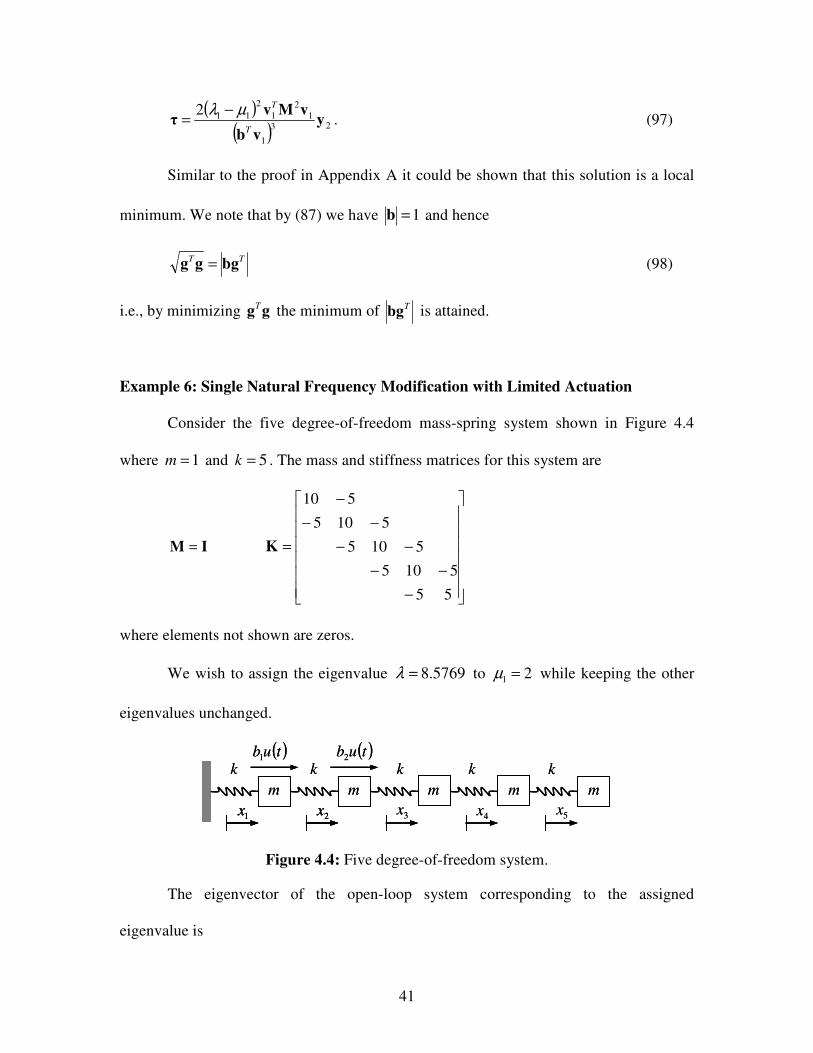
Example 6: Single Natural Frequency Modification with Limited Actuation

Consider the five degree-of-freedom mass-spring system shown in Figure 4.4

where 1=m and 5=k . The mass and stiffness matrices for this system are

IM =

−

−−

−−

−−

−

=

55

5105

5105

5105

510

K

where elements not shown are zeros.

We wish to assign the eigenvalue 5769.8=λ to 21 =µ while keeping the other

eigenvalues unchanged.

Figure 4.4: Five degree-of-freedom system.

The eigenvector of the open-loop system corresponding to the assigned

eigenvalue is

m

k k

m

( )tub1 ( )tub2

1x 2x 3x4x 5x

kkk

m mmm

k k

m

( )tub1 ( )tub2

1x1x 2x2x 3x4x 5x

kkk

m mm

42

( )T4557.03260.05485.01699.05969.0 −−=v .

The graph shown in Figure 4.5 indicates that the minimum of g corresponds to

9618.01 −=b . The associated 2738.02 −=b satisfies the unit norm constraint (89).

We note that

513.32

1

2

1 ==v

v

b

b,

as expected from definition (86) and equation (87).

Figure 4.5: The norm of g as a function of 1b .

We now complete the proof that the solution given by (76)-(77) is the global

minimum of Problem 1. We use the notation 1vv = . By (76) and (77) the minimum norm

associated with the internal solution is

( ) 5.0211vMv

vg

T

I

µλρ

−== . (99)

We now look at the minimal norm solution on the boundary of the domain.

Without loss of generality we may number the degrees of freedom such that an arbitrary

1 b

g

2 1 2 1 b b −−=

1 b

g

2 1 2 1 b b −−=

43

solution on the boundary of the domain is defined by Problem 2 with some nr < . The

boundary minimal norm solution Bρ is then given by (87), (72) and (73)

( ) 5.02

1

11vMv

yg

T

B

µλρ

−== . (100)

From (86) we have vy ≤1 and hence BI ρρ ≤ . It thus follows that the solution

(76)-(77) to Problem 1 is the global minimum. Similar reasoning applies to the proof of

the solution of Problem 2.

Example 7: Checking the Solution on the Physical Domain

Equations (99) and (100) applied to Example 5 give the norm for the interior

minimum

vvb = 6180.1=Iρ ,

and the norms for the boundaries of the physical domain

( )T01±=b 11 v=y 0777.31 =Bρ ,

( )T10 ±=b 21 v=y 9021.12 =Bρ ,

as indicated in Figure 4.3a. The interior minimum is the global one as predicted by the

solution to Problem 1.

Now that it was shown with due mathematical rigor that the solutions given to

Problems 1 and 2 are the minimal norm solutions it is instructive to examine the strength

of the physical argument. The physical domain of parameters is characterize by ℜ∈b

and 1=b . When b is orthogonal to 1v , the problem is not controllable and +∞→g .

We have also the inequality constraint 0>g . It thus follows that there is a minimum

44

somewhere inside the domain or on the boundary of the domain. On the boundary of the

domain some of the elements of b vanish, which means that no actuation is applied to

some of the degrees of freedom. From a physical point of view it is unlikely that the

optimal actuation is achieved without a complete set of actuators, unless by chance where

some of the elements of 1v vanish. The conclusion is that in general the minimum norm

solution is internal to the domain and that it is necessarily defined by the stationary

values of the Lagrangian. Since in Problems 1 and 2 the stationary values are unique up

to a sign change there is no ambiguity in determining the solution.

4.6 Optimal Actuation in the Multiple Natural Frequency Modification

Problem

We now consider the case of optimal actuation where several natural frequencies

are intended to be changed while keeping the rest of the spectrum unaltered. For

simplicity and clarity of exposition we will address the case where 2=m . The extension

to higher dimensions 2>m is straightforward.

Problem 3

Given: M , K , 1µ , 2µ

Find: b , and g such that

{ } { }n

n

kk λλµµµ L3211=

=

and where Tbg attains its minimum.

Here we wish to minimize

( )( )22112211 MvMvMvMvgg ϑϑϑϑ ++= TTT (101)

where kϑ , mk ,.2,1 K= are given by (73), subject to 1=bbT . Note that

45

2

2

1

1

11τ

vbτ

vbg

TT+= (102)

where

( )( )( ) 1

21

21111 Mvτ

λλ

µλµλ

−

−−=

( )( )( ) 2

12

12222 Mvτ

λλ

µλµλ

−

−−= (103)

It thus follows from (102) and (103) that

( ) ( )( ) ( )2

2

22

21

21

2

1

11 2

vb

ττ

vbvb

ττ

vb

ττgg

T

T

TT

T

T

TT ++= . (104)

We define the Lagrangian

( )( ) ( )( ) ( )

bbvb

ττ

vbvb

ττ

vb

ττb

T

T

T

TT

T

T

T

L ξ+++=2

2

22

21

21

2

1

11 2 (105)

where ξ is a Lagrange multiplier. The stationary principle gives

( ) ( ) ( ) ( )( ) ( )

0bvvb

ττv

vbvb

ττv

vbvb

ττv

vb

ττ

b=+−−−−=

∂

∂ξ2

222223

2

2222

21

211

2

2

1

2113

1

11

T

T

TT

T

TT

T

T

TL

. (106)

We define

bb41ˆ ξ= , (107)

and obtain from (106)

( ) ( ) ( ) ( ) ( )( )

bvvbvb

ττ

vb

ττv

vbvb

ττ

vb

ττ ˆˆˆˆˆˆˆ

22

21

21

3

2

221

2

2

1

21

3

1

11 =

++

+

TT

T

T

T

TT

T

T

T

. (108)

We may thus solve (108) for b̂ and obtain the optimal input vector b via the

normalization

b

bb

ˆ

ˆ=

4

b̂=ξ . (109)

46

Note that (108) may be written in the form

bvv =+ 2211 χχ (110)

with the obvious definition of kχ , 2,1=k . Note that (110) indicates that b lies in the

subspace spanned by the vectors 1v and 2v .

By the physical insight gained in Section 4.5 it is clear that the minimal norm

solution is generally internal to the domain and that it is therefore one of the solutions of

(110) by necessity.

Example 8: Multiple Natural Frequency Modification

We consider the mass-spring system shown in Figure 4.2. We wish to assign the

eigenvalues of the system to 11 =µ and 22 =µ with minimal control effort. Since IM =

the bi-orthogonal condition 021 =MvvT implies via (103) that 021 =ττT and the system of

equations (108) reduces to

( ) ( )

bvvb

ττv

vb

ττ ˆˆˆ

23

2

2213

1

11 =+T

T

T

T

. (111)

With

=

3804.0

2351.01τ

−=

2351.0

3804.02τ

and 1v , 2v as given in Example 1, we obtain two solutions to (111)

−=

0946.1

2584.0ˆ

1b ,

−

−=

2584.0

0946.1ˆ

2b .

By (109) the optimal input vector is

−=

9732.0

2298.01b ,

−

−=

2298.0

9732.02b .

47

(a)

1b

g

2

12 1 bb −−=

(b)

1b

g

2

12 1 bb −−=

(c)

1b

g

2

12 1 bb −−=

(a)

1b

g

2

12 1 bb −−=

(b)

1b

g

2

12 1 bb −−=

(c)

1b

g

2

12 1 bb −−=

Figure 4.6: The norm of g as a function of 1b , (a) in the complete physical range

11 1 ≤≤− b , (b) zoom on the left minimum, and (c) zoom on the right minimum.

Figure 4.6a shows the norm of g as a function of 1b in the range of 11 1 ≤≤− b . It

is apparent from the graph that there are two local minima in this complete range. Figures

4.6b and 4.6c zoom on these minima and show the two solutions for the optimal input

vector b obtained above.

4.7 Pole Placement by Optimal Actuation

We now consider the problem of finding the optimal actuation for complete pole

assignment for damped systems. The pole placement problem is formulated in equations

(27)-(28) and (40). Here there are two feedback vectors f and g hence the cost function

η to be minimized involves a given weighting parameter w ,

48

22

gf w+≡η . (112)

The characteristic equation of the closed-loop system is defined as follows

( ) ( ) ( )( )TTsss bgKbfCM −+−+≡ 2detφ (113)

and the problem to be solved is:

Problem 4

Given M , C , K , w , and the eigenvalues of the closed-loop system nsss 221 ,...,,

Find b , f and g

which minimize η

subject to the constraints

( ) 0=ksφ nk 2,..,2,1= (114)

and

1=b . (115)

To solve the problem we define the Lagrangian

( ) ( )∑=

−−+=n

k

kk

TTT swL2

1

0,, φξξ bbggffgfb (116)

where kξ , nk 2,...,1,0= are Lagrange multipliers. The solution to the problem is given by

the set of equations

( )0

b

gfb=

∂

∂ ,,L

( )0

f

gfb=

∂

∂ ,,L

( )0

g

gfb=

∂

∂ ,,L (117)

together with (114) and (115). Note that this set of equations gives 15 +n equations for

the 15 +n unknowns in b , f , g and kξ , nk 2,...,1,0= . The explicit forms of the

equations in (117) are

49

( )

bb

0

2

1

2ξφ

ξ −=∂

∂∑

=

n

k

kk

s,

( )f

f2

2

1

=∂

∂∑

=

n

k

kk

sφξ ,

( )g

gw

sn

k

kk 2

2

1

=∂

∂∑

=

φξ . (118)

A numerically viable method for finding the derivative of a matrix determinant

with respect to a parameter without expanding the determinant by its fundamental

definition is given in Ram [12].

Example 9: Full Eigenvalue Assignment

Consider the open-loop system shown in Figure 4.7 with 5=k , 1=m and

2.0=c . The mass damping and stiffness matrix for this system are:

=

100

020

001

M

−

−

=

000

02.02.0

02.02.0

C

−

−−

−

=

550

51510

01015

K

Figure 4.7: The open-loop system of Example 9.

We wish to assign the eigenvalues of the system to the set

11 −=s , 32 −=s , is 25.04,3 ±−= , is 575.06,5 ±−=

by using optimal actuation with a norm weighting of 1=w .

The sixteen equations defined by (114), (115) and (118) yield two physical

solutions. One solution

−

−

=

0149.0

1637.0

9864.0

b

−

=

9836.1

5344.14

0492.5

f

−

−=

1243.1

5870.6

2817.15

g

with seven Lagrange multipliers

mk

k2

m2k

m

c

mk

k2

m2k

m

c

50

8605.5180 −=ξ , 2791.01 =ξ , 1196.02 −=ξ ,

i0959.01209.04,3 ±−=ξ , i0178.00333.06,5 ±=ξ ,

corresponds to the local minimum 8605.518min =η of the cost function. The graph of η in

the neighborhood of b associated with this solution is shown in Figure 4.8.

The second solution

−=

70740

3998.0

5828.0

.

b ,

−

−=

4637.11

7946.2

3184.2

f

−

−

=

4205.7

0012.14

8479.10

g

with

3758.5130 −=ξ , 3736.01 =ξ , 1403.02 −=ξ ,

i1314.02999.04,3 ±−=ξ , i0191.00351.06,5 ±=ξ ,

corresponds to the global minimum 3758.513min =η of the cost function. The graph of η

in the neighborhood of b associated with the global optimization is shown in Figure 4.9.

1b2b

η

1b2b

η

Figure 4.8: Local minimum of η , 2

2

2

13 1 bbb −−= .

51

1b2b

η

1b2b

η

Figure 4.9: Global minimum of η , 2

2

2

13 1 bbb −−= .

52

CHAPTER 5: DEMONSTRATION WITH UNITS

Previous examples all demonstrated minimization of a cost function, but the true

measure of this method is in the magnitude reduction of control effort. A physical system

can be modeled with units to demonstrate this.

The force selection vector, b, has no units and is merely the multiplication of

control force applied to each degree of freedom. In a physical system using SI units,

mass can be given in units of kilograms, stiffness in units of Newtons per millimeter, and

damping in units of Newtons per millimeter per second. The eigenvalues are frequencies

in units of radians per second, and the eigenvectors are a normalized unit length as

millimeters. The position and velocity are given as millimeters and millimeters per

second, respectively. This means the calculation of q from (38) results in units of

millimeters-1

. Thus, the velocity gain vector, f, from (36) has units of kilograms per

second, and the position gain vector, g, from (37) has units of 103 kilograms per second

squared. The control force, u, would then, from (27), have units of Newtons that are

multiplied by the force selection vector and applied to each degree of freedom. Note that

a 10-3

correction must be applied to the velocity gain multiplication in (27) to account for

the use of millimeters instead of meters. The optimization laid out in this thesis works to

minimize the magnitude of this control force input, u, as well as the magnitude of the

total control effort, b*u.

If Example 9 is run with SI units considered for each of the parameters, the

system can be rewritten as

53

1 0 0

0 2 0

0 0 1

=

M kg

−

−

=

000

02.02.0

02.02.0

C N/mm/s

−

−−

−

=

550

51510

01015

K N/mm.

The optimum force selection vector and feedback gain vectors would then be

0.5828

0.3998

0.7074

= −

b ,

2.3184

2.7946

11.4637

= − −

f kg/s,

10.8479

14.0012

7.4205

−

= −

g kg/s2.

Given an initial position and velocity of

0

1

0

0

=

x mm, 0

0

1

0

=

x& mm/s,

the system will respond with a specific dynamic response and the control system will

bring all masses back to equilibrium by assigning the eigenvalues to the set

11 −=s , 32 −=s , is 25.04,3 ±−= , is 575.06,5 ±−=

as demonstrated in Example 9.

Using the optimal force selection vector and associated gain vectors, the control

input necessary over time is shown in Figure 5.1.

Figure 5.1: Control force input needed to control the system when using the optimal

force selection vector.

54

The peak control input, u, is 15.11 N. The sum of all control inputs for each 0.1-

sec time step from 0 to 20 seconds is 180.65 N. When multiplied by the force selection

vector and distributed across all masses, the magnitude of the total control effort, b*u,

applied over the 20 seconds is 305.31 N.

We can compare these values to an arbitrary force selection vector. For this

example, a force selection vector of equal components is chosen,

1 3 0.57735

1 3 0.57735

0.577351 3

= =

b .

This results in gain vectors

77.66

115.08

145.94

= −

f kg/s,

50.96

138.28

143.99

= −

g kg/s2.

This arbitrary control accomplishes the same pole placement. Under the same

initial conditions as the previous example, the control input over time is shown in Figure

5.2. Note that the y-axis has been increased to accommodate the higher values.

Figure 5.2: Control force input needed to control the system when using the optimal

force selection vector.

55

The peak control input using equally distributed actuation is 86.00 N. The sum of

all control inputs for each 0.1-sec time step from 0 to 20 seconds is 2022.96 N. When

multiplied by the force selection vector and distributed across all masses, the magnitude

of the total control effort, b*u, applied over the 20 seconds is 3503.9 N.

The peak control input of the optimized actuation is 17.6% of the equally

distributed actuation. Also, the total control input of the optimized actuation over the 20

seconds of simulation is also 8.9% of that of the equally distributed actuation. The total

control effort from actuation across all degrees of freedom over the 20 second interval by

the optimized actuation is only 8.7% of the equally distributed actuation.

In the system studied, holding all other parameters and initial conditions to be the

same, using optimal actuation instead of an equally-distributed actuation decreases the

amount of control force necessary to assign the eigenvalues as desired by an order of

magnitude. In this example, there was an 1100 times reduction in control effort needed.

56

CHAPTER 6: CONCLUSIONS

The results show that at least an order of magnitude improvement can be achieved

by paying attention to the open-loop properties of the system and choosing the control

input that is parallel to the eigenvector associated with the eigenvalue to be reassigned.

The term “parallel” in this case can be confusing. Consider a string that is vibrating. In

each mode of vibration, there will be points in the string which experience no deflection,

and there will be other points which experience maximum deflection. If a sensor/actuator

pair is placed at a zero-point, the point with no deflection, there will be no measurable

change in state and thus no control applied. This would be analogous to using a force

selection vector, b, which is orthogonal to an open-loop eigenvector, resulting in an

uncontrollable system. If the sensor/actuator pair is moved to a maximum-point, where

there is maximum deflection, the control is able to act directly at the point where it is

needed most. This is analogous to using the optimal force selection vector which is

parallel to an open-loop eigenvector. In the case where more than one eigenvalue is to be

reassigned, the optimal force selection vector will be in the subspace of the associated

eigenvectors and as near to parallel to all of them as possible. The results have shown

this to be true for damped and undamped systems and even systems with limited

actuation. Use of Lagrange multipliers has been developed to find the optimal control

input in the case of a damped system with full pole placement. All examples result in

minimal control effort to accomplish the desired pole assignment.

Due to the nature of the mathematical equations, this theory could be explored for

use in more than just mechanical systems. Simple electrical systems use a similar

57

differential equation, thus this theory may apply to the problem of controlling

fluctuations in current in such systems. Future research could use a simple electrical

circuit to prove the theory through experimentation.

There is also possible application of this theory in vibration enhancement instead

of vibration control. It is usually desirable to shift the eigenvalues of a system to the left-

half of the complex plane, in order to reduce vibration. However, in the field of energy

harvesting, it may be desirable to increase vibration by moving the poles of a system

further towards the right. The theory presented here works to minimize the control effort

needed, no matter what value is chosen for the new eigenvalues.

It should be noted that this work is still theoretical and has not been demonstrated

outside of computer simulation. Future work is needed to test the theory with a physical

demonstration.

58

REFERENCES

Alkhatib, Rabih, and M. F. Golnaraghi. "Active Structural Vibration Control: A

Review." The Shock and Vibration Digest 35, no. 5 (2003): 367-83.

Bai, Z.J., B.N. Datta and J.W. Wang. “Robust and minimum norm partial quadratic

eigenvalue assignment in vibrating systems: A new optimization approach.”

Mechanical Systems and Signal Processing 24 (2010): 766-783.

Balas, Mark J. "Direct Velocity Feedback Control of Large Space Structures." Journal of

guidance and control 2, no. 3 (1978): 252-53.

Chang, Chih-Chen, and Lung-On Yu. "The Application of Optimal Pole Placement

Technique in Structural Control." Active control of vibration and noise 93 (1996):

161-71.

D'Azzo, John J., and Constantine H. Houpis. Linear Control System Analysis and Design:

Conventional and Modern. 4th

ed. New York, NY: McGraw-Hill, 1995.

Datta, Biswa N., Sylvan Elhay, and Yitshak M. Ram. "Orthogonality and Partial Pole

Assignment for the Symmetric Definite Quadratic Pencil." Linear algebra and its

applications 257 (1997): 29-48.

Datta, B.N. and V. Sokolov. “Quadratic inverse eigenvalue problems, active vibration

control and model updating.” Applied and Computational Mathematics 8 (2009):

170-191.

Datta, Biswa N., and Daniil R. Sarkissian. "Partial Eigenvalue Assignment in Linear

Systems: Existence, Uniqueness and Numerical Solution." Paper presented at the

15th International symposium on the mathematical theory of networks and

systems, University of Notre Dame, South Bend, IN, August 14, 2002 2002.

Dosch, Jeffrey J., Daniel J. Inman, and Ephrahim Garcia. "A Self-Sensing Piezoelectric

Actuator for Collocated Control." Journal of intelligent material systems and

structures 3, no. 1 (1992): 166-85.

Elishakoff, I.. “A selective review of direct, semi-inverse and inverse eigenvalue

problems for structures described by differential equations with variable

coefficients.” Archives of Computational Methods in Engineering 7 (2000): 451-

526.

Franklin, Gene F., J. David Powell, and Abbas Emami-Naeini. Feedback Control of

Dynamic Systems. 3rd

ed. Reading, MA: Addison-Wesley, 1994.

59

Gao, W., J. J. Chen, H. B. Ma, and X. S. Ma. "Optimal Placement of Active Bars in

Active Vibration Control for Piezoelectric Intelligent Truss Structures with

Random Parameters." Computers and structures 81 (2003): 53-60.

Golub, G. H. and C. F. Van Loan. Matrix Computations. 2nd

ed. Baltimore, MD: The

Johns Hopkins University Press, 1989.

Hong, Seongil, Chul H. Park, and Hyun C. Park. "Vibration Control of Beams Using

Multiobjective State-Feedback Control." Smart materials and structures 15

(2006): 157-63.

Jiang, Dan-chi, and J. B. Moore. "Least Squares Pole Assignment by Memoryless Output

Feedback." Systems and control letters 29 (1996): 31-42.

Karbassi, S. M. "An Algorithm for Minimizing the Norm of State Feedback Controllers

in Eigenvalue Assignment." Computers and mathematics with applications 41

(2001): 1317-26.

Kimura, Hidenori. "Pole Assignment by Gain Output Feedback." IEEE transactions on

automatic control 20, no. 4 (1975): 509-16.

Korn, G.A. and T.M. Korn. Mathematical Handbook for Scientists and Engineers. 2nd

ed.

New York, NY: McGraw Hill Book Company, 1968.

Lam, James, and Wei-Yong Yan. "Pole Assignment with Optimal Spectral

Conditioning." Systems and control letters 29 (1997): 241-53.

Lawther, R. “Assessing how changes to a structure can create gaps in the natural

frequency spectrum.” International Journal of Solids and Structures 44 (2007):

614-635.

Matsuzaki, Yuji, Tadashige Ikeda, and Christian Boller. "New Technological

Development of Passive and Active Vibration Control: Analysis and Test." Smart

materials and structures 14 (2005): 343-48.

McMillan, A.J. and A.J. Keane. “Shifting resonances from a frequency band by applying

concentrated masses to a thin rectangular plate.” Journal of Sound and Vibration

192 (1996): 549–562.

Mierovitch, Leonard. Fundamentals of Vibrations. New York, NY: McGraw-Hill, 2001.

Miminis, George S., and Chris C. Paige. "A Direct Algorithm for Pole Assignment of

Time-Invariant Multi-Input Linear Systems Using State Feedback." Automatica

24, no. 3 (1988): 343-56.

Mottershead, John E., and Yitshak M. Ram. "Inverse Eigenvalue Problems in Vibration

Absorption: Passive Modification and Active Control." Mechanical systems and

signal processing 20, no. 1 (2006): 5-44.

60

Qian, Jiang, and Shufang Xu. "Robust Partial Eigenvalue Assignment Problem for the

Second-Order System." Journal of sound and vibration 282 (2005): 937-48.

Ram, Y. M. “Enlarging a spectral gap by structural modification.” Journal of Sound and

Vibration 176 (1994): 225-234.

Ram, Y. M. “A method for finding repeated roots in transcendental eigenvalue

problems.” Proceedings of the Institution of Mechanical Engineers, Part C,

Journal of Mechanical Engineering Science 222 (2008): 1665-1671.

Ram, Y. M. and J. J. Blech. “The dynamic behaviour of a vibratory system after

modification.” Journal of Sound and Vibration 150 (1991): 357-370.

Ram, Y. M. and S. Elhay. “Pole assignment in vibratory systems by multi-input control.”

Journal of Sound and Vibration 230 (2000): 309-321.

Ram, Y. M., and D. J. Inman. "Optimal Control for Vibrating Systems." Mechanical

systems and signal processing 13, no. 6 (1999): 879-92.

Schulz, G., and G. Heimbold. "Dislocated Actuator/Sensor Positioning and Feedback

Design for Flexible Structures." Journal of guidance, control, and dynamics 6

(1983): 361-67.

Song, Y. D., and T. L. Mitchell. "Active Damping Control of Vibrational Systems." IEEE

transactions on aerospace and electronic systems 32, no. 2 (1996): 569-77.

Vasques, C. M. A., and J. Dias Rodrigues. "Active Vibration Control of Smart

Piezoelectric Beams: Comparison of Classical and Optimal Feedback Control

Strategies." Computers and structures 84 (2006): 1402-14.

Xu, S.F. and J. Qian. “Orthogonal basis selection method for robust partial eigenvalue

assignment problem in second-order control systems.” Journal of Sound and

Vibration 317 (2008): 1-19.

Yang, S. M., and Y. J. Lee. "Optimization of Non-Collocated Sensor/Actuator Location

and Feedback Gain in Control Systems." Smart materials and structures 2 (1993):

96-102.

Zhang, Tianli, Chengbao Jiang, Hu Zhang, and Huibin Xu. "Giant Magnetostrictive

Actuators for Active Vibration Control." Smart materials and structures 13

(2004): 473-77.

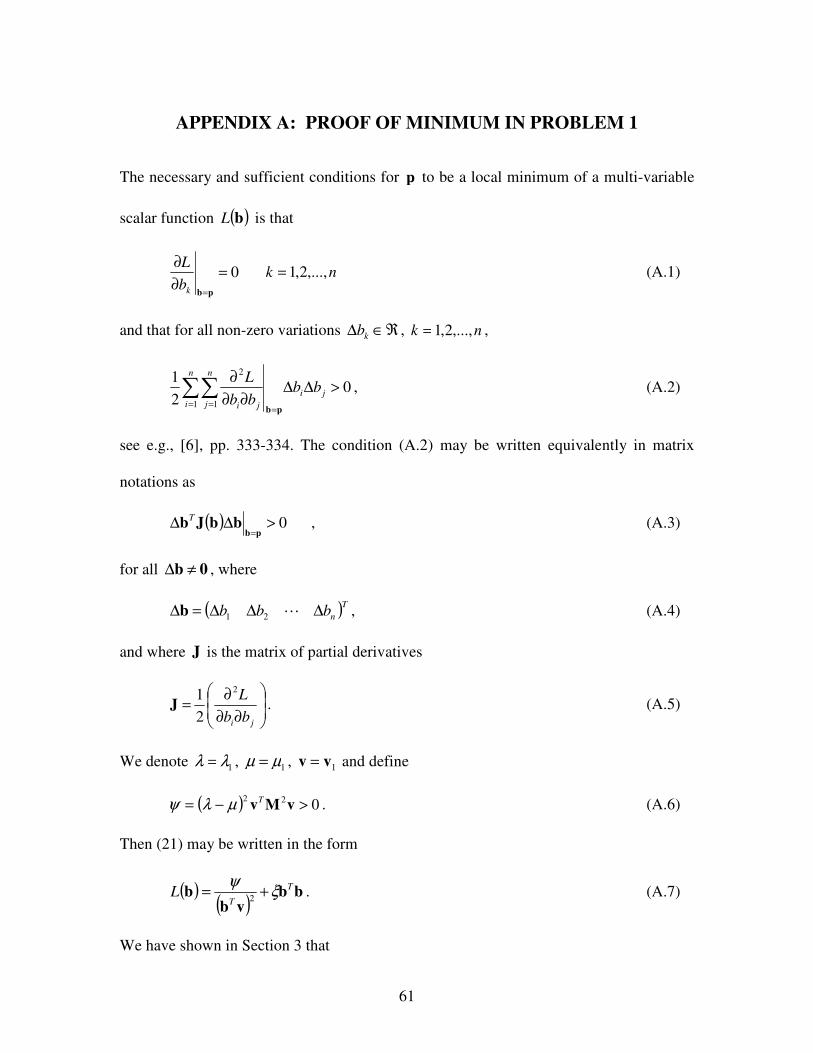
61

APPENDIX A: PROOF OF MINIMUM IN PROBLEM 1

The necessary and sufficient conditions for p to be a local minimum of a multi-variable

scalar function ( )bL is that

0=∂

∂

=pbkb

L nk ,...,2,1= (A.1)

and that for all non-zero variations ℜ∈∆ kb , nk ,...,2,1= ,

02

1

1 1

2

>∆∆∂∂

∂∑∑

= ==

ji

n

i

n

j ji

bbbb

L

pb

, (A.2)

see e.g., [6], pp. 333-334. The condition (A.2) may be written equivalently in matrix

notations as

( ) 0>∆∆=pb

bbJbT , (A.3)

for all 0b ≠∆ , where

( )T

nbbb ∆∆∆=∆ L21b , (A.4)

and where J is the matrix of partial derivatives

∂∂

∂=

ji bb

L2

2

1J . (A.5)

We denote 1λλ = , 1µµ = , 1vv = and define

( ) 022>−= vMv

Tµλψ . (A.6)

Then (21) may be written in the form

( )( )

bbvb

bT

TL ξ

ψ+=

2. (A.7)

We have shown in Section 3 that

62

v

vb = , (A.8)

satisfies the n equations in (A.1). To show that the condition in (A.2) is also satisfied we

differentiate

( ) jT

j

j

bv

b

Lξ

ψ2

23

+−

=∂

∂

vb, (A.9)

and obtain by second differentiation

≠

=+=

∂∂

∂

jivv

jivv

bb

L

ji

ji

jiγ

ξγ

2

222

, (A.10)

where

( )4

3

vbT

ψγ = . (A.11)

From (A.5) we have

TvvIJ γξ += . (A.12)

With b chosen as in (A.8) Equation (A.11) gives

( )

03

2>=

vvT

ψγ , (A.13)

by virtue of (A.6). From (24)

( ) ( )

022

>−

=vv

vMvT

Tµλξ . (A.14)

It thus follows from the monotonicity property of the eigenvalues of symmetric

matrices that J is a positive definite matrix, see e.g., [5], p. 462. The condition (A.3) is

therefore satisfied for all 0b ≠∆ , and the solution (A.8) is a local minimum.

63

APPENDIX B: COMPUTER FILES USED IN EXAMPLES

MATLAB file for Example 1 clear all; % input system parameters n=2; % two-dimensional system m1=1; m2=2; % define mass of each dimension k1=5; k2=10; % define spring constants % k1 is spring from ground to mass 1, % k2 is from mass 1 to mass 2 c1=0; c2=0.2; % define damping constants % c1 is dashpot from ground to mass 1, % c2 is from mass 1 to mass 2 % % begin calculations I=eye(n); % identity matrix O=zeros(n,n); % zero matrix M=[m1 0; % mass matrix 0 m2]; C=[c1+c2 -c2; % damping matrix -c2 c2]; K=[k1+k2 -k2; % spring matrix -k2 k2]; A=[O I; % first-order realization -K O]; B=[I O; C M]; [U,S]=eig(A,B); % eigenvalues and eigenvectors % % For verification % s=-0.1472 -+ 4.3170i,-0.0028 -+ 1.1575i % v=0.0263 -+ 0.1995i, 0.0082 -+ 0.6269i % -0.0114 +- 0.0728i, 0.0055 -+ 0.8563i % % Initial conditions x0=[1 0]'; % define initial position xdot0=[0 1]'; % define initial velocity a=U\[x0;xdot0]; % calculate coefficients of solution % % For verification % a=[0.0025 +- 1.9711i, 0.3872 +- 0.1652i]' % % Calculate solution for each time-step k=0; for j=0:0.1:100 % define time range and step k=k+1; t(k)=j; % time x1(k)=0; % initialize positions and velocities of masses x2(k)=0; xdot1(k)=0; xdot2(k)=0; for i=1:2*n % begin calculations for time step x1(k)=x1(k)+a(i)*U(1,i)*exp(S(i,i)*j); % position of mass 1 x2(k)=x2(k)+a(i)*U(2,i)*exp(S(i,i)*j); % position of mass 2

64

xdot1(k)=xdot1(k)+a(i)*S(i,i)*U(1,i)*exp(S(i,i)*j); % velocity

of mass 1 xdot2(k)=xdot2(k)+a(i)*S(i,i)*U(2,i)*exp(S(i,i)*j); % velocity

of mass 2 end end % remove discretization errors by rounding off any imaginary parts less % than tolerance tol=1e-10; % define tolerance setting if imag(x1)<tol x1=real(x1); end if imag(x2)<tol x2=real(x2); end if imag(xdot1)<tol xdot1=real(xdot1); end if imag(xdot2)<tol xdot2=real(xdot2); end

% RESULTS - POSITION AND VELOCITY OF BOTH MASSES frame=401; % plot up to t=40 subplot(2,2,1) % top left box shows plot of mass 1 position plot(t(1:frame),x1(1:frame),'-r','LineWidth',2) axis([0 40 -1.5 1.5]) xlabel('Time, t') ylabel('Position, x') title('Position of Mass 1 From Equilibrium')

subplot(2,2,2) % top right box shows plot of mass 2 position plot(t(1:frame),x2(1:frame),'-r','LineWidth',2) axis([0 40 -1.5 1.5]) xlabel('Time, t') ylabel('Position, x') title('Position of Mass 2 From Equilibrium')

subplot(2,2,3) % bottom left box shows plot of mass 1 velocity plot(t(1:frame),xdot1(1:frame),'-b','LineWidth',2) axis([0 40 -3 3]) xlabel('Time, t') ylabel('Velocity, dot{x}') title('Velocity of Mass 1')

subplot(2,2,4) % bottom right box shows plot of mass 2 velocity plot(t(1:frame),xdot2(1:frame),'-b','LineWidth',2) axis([0 40 -3 3]) xlabel('Time, t') ylabel('Velocity, dot{x}') title('Velocity of Mass 2')

MATLAB file for Example 2 clear all; % input system parameters

65

n=2; % two-dimensional system m1=1; m2=2; % define mass of each dimension k1=5; k2=10; % define spring constants % k1 is spring from ground to mass 1, % k2 is from mass 1 to mass 2 c1=0; c2=0.2; % define damping constants % c1 is dashpot from ground to mass 1, % c2 is from mass 1 to mass 2 % % calculate open loop eigenvalues I=eye(n); % identity matrix O=zeros(n,n); % zero matrix M=[m1 0; % mass matrix 0 m2]; C=[c1+c2 -c2; % damping matrix -c2 c2]; K=[k1+k2 -k2; % spring matrix -k2 k2]; Ao=[O I; -K O]; Bo=[I O; C M]; [Uo,So]=eig(Ao,Bo); b=[2 1]'; % arbitrary control selection vector i=sqrt(-1); for k=1:2*n vo(:,k)=Uo(1:n,k); % Uo is given as normalized set end; so=[So(1,1); So(2,2); So(3,3); So(4,4)]; % open loop eigenvectors mu=[so(1); so(2); -1-i; -1+i]; % define new eigenvalues to be assigned Num1=((mu(3)-so(3))/so(3))*((mu(4)-so(3))/(so(4)-so(3))); Num2=((mu(4)-so(4))/so(4))*((mu(3)-so(4))/(so(3)-so(4))); Den1=b'*vo(:,3); Den2=b'*vo(:,4); q(1,1)=Num1./Den1; q(2,1)=Num2./Den2; f=M*vo(:,3:4)*diag(so(3:4))*q; g=-K*vo(:,3:4)*q;% solve for new eigenvalues of the system A=[O I; % first-order realization including control -(K-b*g') O]; B=[I O; (C-b*f') M]; [U,S]=eig(A,B); % eigenvalues and eigenvectors % % Initial conditions x0=[1 0]'; % define initial position xdot0=[0 1]'; % define initial velocity a=U\[x0;xdot0]; % calculate coefficients of solution % % Calculate solution for each time-step k=0; for j=0:0.1:100 % define time range and step k=k+1; t(k)=j; % time x1(k)=0; % initialize positions and velocities of masses x2(k)=0; xdot1(k)=0;

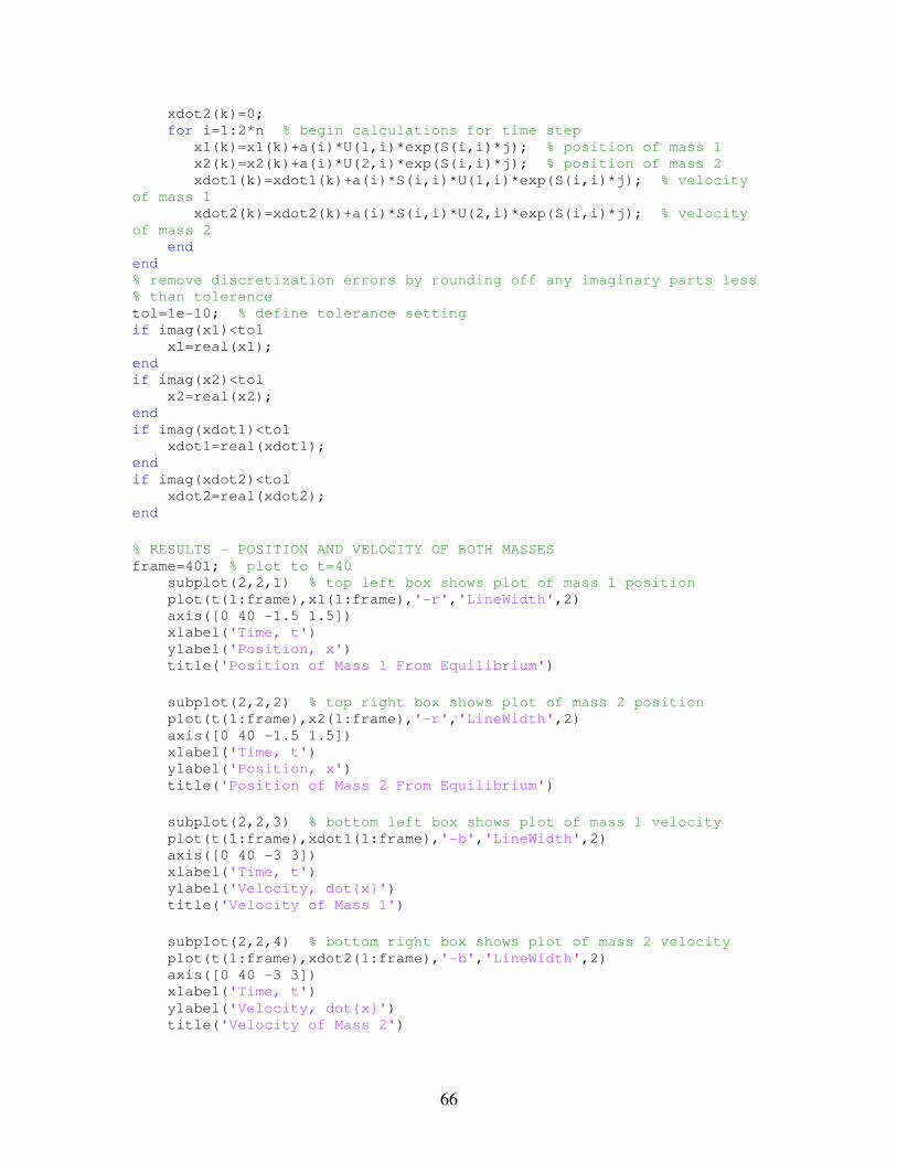
66

xdot2(k)=0; for i=1:2*n % begin calculations for time step x1(k)=x1(k)+a(i)*U(1,i)*exp(S(i,i)*j); % position of mass 1 x2(k)=x2(k)+a(i)*U(2,i)*exp(S(i,i)*j); % position of mass 2 xdot1(k)=xdot1(k)+a(i)*S(i,i)*U(1,i)*exp(S(i,i)*j); % velocity

of mass 1 xdot2(k)=xdot2(k)+a(i)*S(i,i)*U(2,i)*exp(S(i,i)*j); % velocity

of mass 2 end end % remove discretization errors by rounding off any imaginary parts less % than tolerance tol=1e-10; % define tolerance setting if imag(x1)<tol x1=real(x1); end if imag(x2)<tol x2=real(x2); end if imag(xdot1)<tol xdot1=real(xdot1); end if imag(xdot2)<tol xdot2=real(xdot2); end

% RESULTS - POSITION AND VELOCITY OF BOTH MASSES frame=401; % plot to t=40 subplot(2,2,1) % top left box shows plot of mass 1 position plot(t(1:frame),x1(1:frame),'-r','LineWidth',2) axis([0 40 -1.5 1.5]) xlabel('Time, t') ylabel('Position, x') title('Position of Mass 1 From Equilibrium')

subplot(2,2,2) % top right box shows plot of mass 2 position plot(t(1:frame),x2(1:frame),'-r','LineWidth',2) axis([0 40 -1.5 1.5]) xlabel('Time, t') ylabel('Position, x') title('Position of Mass 2 From Equilibrium')

subplot(2,2,3) % bottom left box shows plot of mass 1 velocity plot(t(1:frame),xdot1(1:frame),'-b','LineWidth',2) axis([0 40 -3 3]) xlabel('Time, t') ylabel('Velocity, dot{x}') title('Velocity of Mass 1')

subplot(2,2,4) % bottom right box shows plot of mass 2 velocity plot(t(1:frame),xdot2(1:frame),'-b','LineWidth',2) axis([0 40 -3 3]) xlabel('Time, t') ylabel('Velocity, dot{x}') title('Velocity of Mass 2')

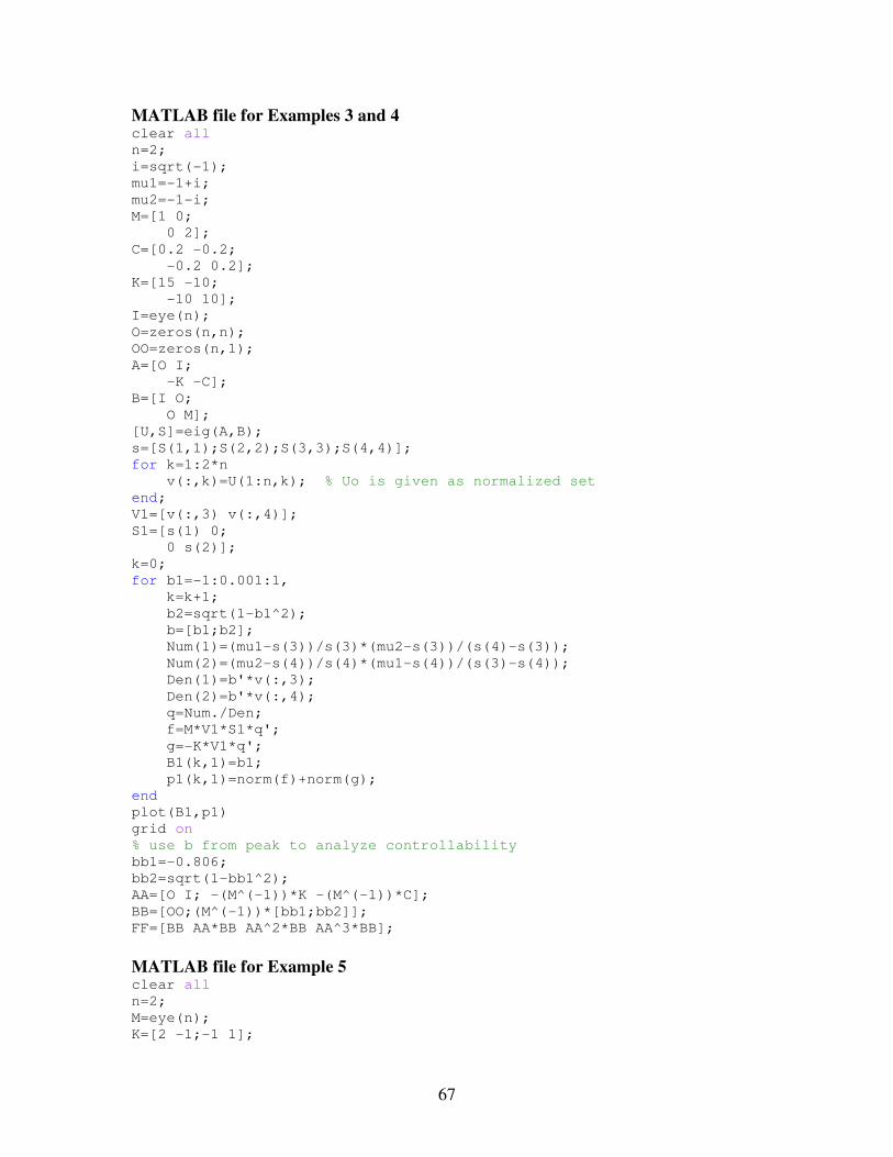
67

MATLAB file for Examples 3 and 4 clear all n=2; i=sqrt(-1); mu1=-1+i; mu2=-1-i; M=[1 0; 0 2]; C=[0.2 -0.2; -0.2 0.2]; K=[15 -10; -10 10]; I=eye(n); O=zeros(n,n); OO=zeros(n,1); A=[O I; -K -C]; B=[I O; O M]; [U,S]=eig(A,B); s=[S(1,1);S(2,2);S(3,3);S(4,4)]; for k=1:2*n v(:,k)=U(1:n,k); % Uo is given as normalized set end; V1=[v(:,3) v(:,4)]; S1=[s(1) 0; 0 s(2)]; k=0; for b1=-1:0.001:1, k=k+1; b2=sqrt(1-b1^2); b=[b1;b2]; Num(1)=(mu1-s(3))/s(3)*(mu2-s(3))/(s(4)-s(3)); Num(2)=(mu2-s(4))/s(4)*(mu1-s(4))/(s(3)-s(4)); Den(1)=b'*v(:,3); Den(2)=b'*v(:,4); q=Num./Den; f=M*V1*S1*q'; g=-K*V1*q'; B1(k,1)=b1; p1(k,1)=norm(f)+norm(g); end plot(B1,p1) grid on % use b from peak to analyze controllability bb1=-0.806; bb2=sqrt(1-bb1^2); AA=[O I; -(M^(-1))*K -(M^(-1))*C]; BB=[OO;(M^(-1))*[bb1;bb2]]; FF=[BB AA*BB AA^2*BB AA^3*BB];

MATLAB file for Example 5 clear all n=2; M=eye(n); K=[2 -1;-1 1];

68

[U,S]=eig(K,M); ss=diag(S); mu1=2; mu2=ss(2); mu=[mu1;mu2]; k=0; for b1=-1:0.001:1, k=k+1; b2=sqrt(1-b1^2); b=[b1;b2]; g=place(K,b,mu); s=eig(K-b*g,M); B1(k,1)=b1; B2(k,1)=b2; G1(k,1)=g(1); G2(k,1)=g(2); N(k,1)=norm(g); end subplot(2,2,1) semilogy(B1,N) text(-0.5,10^3,'$b_{2}=\sqrt{1-

b_{1}^{2}}$','Interpreter','latex','FontSize',12) title('(a)') xlabel('$b_{1}$','Interpreter','latex','FontSize',12) text(-1.5,10^2,'$\left | \mathbf{g} \right

|$','Interpreter','latex','FontSize',12) subplot(2,2,2) plot(B1,N) text(0.25,1.88,'$b_{2}=\sqrt{1-

b_{1}^{2}}$','Interpreter','latex','FontSize',12) title('(b)') xlabel('$b_{1}$','Interpreter','latex','FontSize',12) axis([0 1 1.5 2])

MATLAB file for Example 6 clear all n=5;m=2;i=1;j=2; mu=2; M=eye(n); E=eye(n)-diag(ones(n-1,1),1); K=5*E*E'; [U,S]=eig(K,M); s1=S(3,3); u1=U(:,3); k=0; for b1=-1:0.0001:1, k=k+1; b2=-sqrt(1-b1^2); b=[zeros(i-1,1);b1;zeros(j-i-1,1);b2;zeros(n-j,1)]; g=(s1-mu)/(b'*u1); f=g*M*u1; B1(k,1)=b1; B2(k,1)=b2; Nf(k,1)=norm(f); end subplot(2,2,1)

69

plot(B1,Nf) axis([-1 -0.8 10.5 11.5]) title(' ') text(-0.965,11.25,'$b_{2}=-\sqrt{1-

b_{1}^{2}}$','Interpreter','latex','FontSize',12) xlabel('$b_{1}$','Interpreter','latex','FontSize',12) text(-1.05,11,'$\left | \mathbf{g} \right

|$','Interpreter','latex','FontSize',12) text(-0.78,10.5,' ')

MATLAB file for Example 8 clear all n=2; M=eye(n); K=[2 -1;-1 1]; [U,S]=eig(K,M); ss=diag(S); mu1=1; mu2=2; mu=[mu1;mu2]; k=0; for b1=-1:0.001:1, k=k+1; b2=-sqrt(1-b1^2); b=[b1;b2]; g=place(K,b,mu); s=eig(K-b*g,M); B1(k,1)=b1; B2(k,1)=b2; G1(k,1)=g(1); G2(k,1)=g(2); N(k,1)=norm(g); end subplot(2,2,1.5) semilogy(B1,N) text(-0.38,9.9^3,'$b_{2}=\sqrt{1-

b_{1}^{2}}$','Interpreter','latex','FontSize',12) title('(a)') xlabel('$b_{1}$','Interpreter','latex','FontSize',12) text(-1.55,10^1,'$\left | \mathbf{g} \right

|$','Interpreter','latex','FontSize',12) text(1.4,10^-2,' ') subplot(2,2,3) plot(B1,N) axis([-1 -0.85 0.8 1.2]) text(-0.97,1.1,'$b_{2}=\sqrt{1-

b_{1}^{2}}$','Interpreter','latex','FontSize',12) title('(b)') xlabel('$b_{1}$','Interpreter','latex','FontSize',12) text(-1.04,0.95,'$\left | \mathbf{g} \right

|$','Interpreter','latex','FontSize',12) subplot(2,2,4) plot(B1,N) axis([0 0.5 0.8 1.2]) text(0.11,1.1,'$b_{2}=\sqrt{1-

b_{1}^{2}}$','Interpreter','latex','FontSize',12)

70

title('(c)') xlabel('$b_{1}$','Interpreter','latex','FontSize',12) text(-0.12,0.95,'$\left | \mathbf{g} \right

|$','Interpreter','latex','FontSize',12) text(0.6,0.8,' ')

MAPLE file for Example 9 > restart; > with(LinearAlgebra):

> Digits:=16: > M:=<<1 | 0 | 0> , <0 | 2 | 0> , <0 | 0 | 1>>:

> K:=<<15 | -10 | 0> , <-10 | 15 | -5> , <0 | -5 | 5>>:

> C:=<<0.2 | -0.2 | 0> , <-0.2 | 0.2 | 0> , <0 | 0 | 0>>: > bf:=<<b1*f1 | b1*f2 | b1*f3> , <b2*f1 | b2*f2 | b2*f3> , <b3*f1 |

b3*f2 | b3*f3>>: > bg:=<<b1*g1 | b1*g2 | b1*g3> , <b2*g1 | b2*g2 | b2*g3> , <b3*g1 |

b3*g2 | b3*g3>>: > eta:=(f1^2+f2^2+f3^2)+a*(g1^2+g2^2+g3^2): > QP1:=s1^2*M+s1*(C-bf)+K-bg:

> QP2:=s2^2*M+s2*(C-bf)+K-bg: > QP3:=s3^2*M+s3*(C-bf)+K-bg:

> QP4:=s4^2*M+s4*(C-bf)+K-bg: > QP5:=s5^2*M+s5*(C-bf)+K-bg: > QP6:=s6^2*M+s6*(C-bf)+K-bg:

> D_QP1:=Determinant(QP1):

> D_QP2:=Determinant(QP2):

> D_QP3:=Determinant(QP3): > D_QP4:=Determinant(QP4): > D_QP5:=Determinant(QP5):

> D_QP6:=Determinant(QP6): > L:=eta-p0*(b1^2+b2^2+b3^2)-p1*D_QP1-p2*D_QP2-p3*D_QP3-p4*D_QP4-

p5*D_QP5-p6*D_QP6: > s1:=-1:s2:=-3:s3:=-0.5+2*I:s4:=-0.5-2*I:s5:=-0.75+5*I:s6:=-0.75-

5*I:a:=1:

> Eq1:=diff(L,b1): > Eq2:=diff(L,b2):

> Eq3:=diff(L,b3): > Eq4:=diff(L,f1): > Eq5:=diff(L,f2):

> Eq6:=diff(L,f3): > Eq7:=diff(L,g1):

> Eq8:=diff(L,g2):

> Eq9:=diff(L,g3): > Eq10:=D_QP1:

> Eq11:=D_QP2: > Eq12:=D_QP3:

> Eq13:=D_QP4: > Eq14:=D_QP5: > Eq15:=D_QP6:

> Eq16:=b1^2+b2^2+b3^2-1:

>

fsolve({Eq1,Eq2,Eq3,Eq4,Eq5,Eq6,Eq7,Eq8,Eq9,Eq10,Eq11,Eq12,Eq13,Eq14,Eq

15,Eq16},{b1=0.5795,b2=-

0.4053,b3=0.7070,f1,f2,f3,g1,g2,g3,p0,p1,p2,p3,p4,p5,p6})

MATLAB file for Example 9 – first graphic

71

clear all; n=3; i=sqrt(-1); M=diag([1 2 1]); C=[0.2 -0.2 0; -0.2 0.2 0; 0 0 0]; K=[15 -10 0; -10 15 -5; 0 -5 5]; s=[-1;-3;-0.5+2*i;-0.5-2*i;-0.75+5*i;-0.75-5*i]; % b=[-0.9863909563940264;-0.1637371834322245;0.01493371707780675]; % b=[-0.9845047747761751;-0.1746871909092368;0.01532102395901377]; % b=[0.5827969264810778;-0.3998426084738319;0.7074416095573197]; dd=0.000001; k1=0; for b1=-0.98648:dd:-0.9863, k1=k1+1; k2=0; for b2=-0.16378:dd:-0.1636, k2=k2+1; b3=sqrt(1-b1^2-b2^2); b=[b1;b2;b3]; A=[zeros(n,n) eye(n); -inv(M)*K -inv(M)*C]; gf=place(A,-[zeros(n,1);inv(M)*b],s); g=gf(1:n)'; f=gf(n+1:2*n)'; k=1; NN(k2,k1)=f'*f+g'*g; B2(k2,1)=b2; end B1(k1,1)=b1; end mesh(B1,B2,NN) ylabel('$b_{2}$','Interpreter','latex','FontSize',12) xlabel('$b_{1}$','Interpreter','latex','FontSize',12) zlabel('$\eta $','Interpreter','latex','FontSize',12) set(get(gca,'ZLabel'),'Rotation',0.0)

MATLAB file for Example 9 – second graphic clear all; n=3; i=sqrt(-1); M=diag([1 2 1]); C=[0.2 -0.2 0; -0.2 0.2 0; 0 0 0]; K=[15 -10 0; -10 15 -5; 0 -5 5]; s=[-1;-3;-0.5+2*i;-0.5-2*i;-0.75+5*i;-0.75-5*i]; % b=[-0.9863909563940264;-0.1637371834322245;0.01493371707780675]; % b=[-0.9845047747761751;-0.1746871909092368;0.01532102395901377]; % b=[0.5827969264810778;-0.3998426084738319;0.7074416095573197]; dd=0.0025;

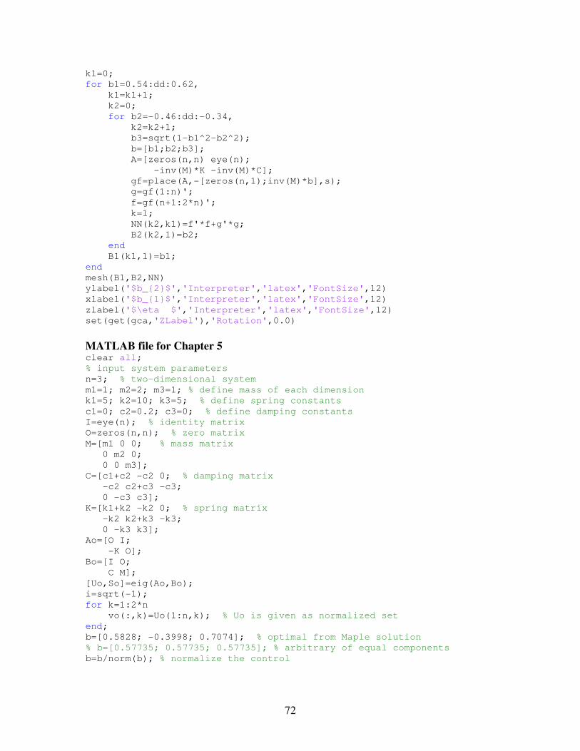
72

k1=0; for b1=0.54:dd:0.62, k1=k1+1; k2=0; for b2=-0.46:dd:-0.34, k2=k2+1; b3=sqrt(1-b1^2-b2^2); b=[b1;b2;b3]; A=[zeros(n,n) eye(n); -inv(M)*K -inv(M)*C]; gf=place(A,-[zeros(n,1);inv(M)*b],s); g=gf(1:n)'; f=gf(n+1:2*n)'; k=1; NN(k2,k1)=f'*f+g'*g; B2(k2,1)=b2; end B1(k1,1)=b1; end mesh(B1,B2,NN) ylabel('$b_{2}$','Interpreter','latex','FontSize',12) xlabel('$b_{1}$','Interpreter','latex','FontSize',12) zlabel('$\eta $','Interpreter','latex','FontSize',12) set(get(gca,'ZLabel'),'Rotation',0.0)

MATLAB file for Chapter 5 clear all; % input system parameters n=3; % two-dimensional system m1=1; m2=2; m3=1; % define mass of each dimension k1=5; k2=10; k3=5; % define spring constants c1=0; c2=0.2; c3=0; % define damping constants I=eye(n); % identity matrix O=zeros(n,n); % zero matrix M=[m1 0 0; % mass matrix 0 m2 0; 0 0 m3]; C=[c1+c2 -c2 0; % damping matrix -c2 c2+c3 -c3; 0 -c3 c3]; K=[k1+k2 -k2 0; % spring matrix -k2 k2+k3 -k3; 0 -k3 k3]; Ao=[O I; -K O]; Bo=[I O; C M]; [Uo,So]=eig(Ao,Bo); i=sqrt(-1); for k=1:2*n vo(:,k)=Uo(1:n,k); % Uo is given as normalized set end; b=[0.5828; -0.3998; 0.7074]; % optimal from Maple solution % b=[0.57735; 0.57735; 0.57735]; % arbitrary of equal components b=b/norm(b); % normalize the control

73

s=[So(1,1); So(2,2); So(3,3); So(4,4); So(5,5); So(6,6)]; % set of

open-loop eigenvalues mu=[-1; -3; -0.5+2*i; -0.5-2*i; -0.75+5*i; -0.75-5*i]; % define new

eigenvalues to be assigned Num1=((mu(1)-s(1))/s(1))*((mu(2)-s(1))/(s(2)-s(1)))*((mu(3)-

s(1))/(s(3)-s(1)))*((mu(4)-s(1))/(s(4)-s(1)))*((mu(5)-s(1))/(s(5)-

s(1)))*((mu(6)-s(1))/(s(6)-s(1))); Num2=((mu(2)-s(2))/s(2))*((mu(1)-s(2))/(s(1)-s(2)))*((mu(3)-

s(2))/(s(3)-s(2)))*((mu(4)-s(2))/(s(4)-s(2)))*((mu(5)-s(2))/(s(5)-

s(2)))*((mu(6)-s(2))/(s(6)-s(2))); Num3=((mu(3)-s(3))/s(3))*((mu(1)-s(3))/(s(1)-s(3)))*((mu(2)-

s(3))/(s(2)-s(3)))*((mu(4)-s(3))/(s(4)-s(3)))*((mu(5)-s(3))/(s(5)-

s(3)))*((mu(6)-s(3))/(s(6)-s(3))); Num4=((mu(4)-s(4))/s(4))*((mu(1)-s(4))/(s(1)-s(4)))*((mu(2)-

s(4))/(s(2)-s(4)))*((mu(3)-s(4))/(s(3)-s(4)))*((mu(5)-s(4))/(s(5)-

s(4)))*((mu(6)-s(4))/(s(6)-s(4))); Num5=((mu(5)-s(5))/s(5))*((mu(1)-s(5))/(s(1)-s(5)))*((mu(2)-

s(5))/(s(2)-s(5)))*((mu(3)-s(5))/(s(3)-s(5)))*((mu(4)-s(5))/(s(4)-

s(5)))*((mu(6)-s(5))/(s(6)-s(5))); Num6=((mu(6)-s(6))/s(6))*((mu(1)-s(6))/(s(1)-s(6)))*((mu(2)-

s(6))/(s(2)-s(6)))*((mu(3)-s(6))/(s(3)-s(6)))*((mu(4)-s(6))/(s(4)-

s(6)))*((mu(5)-s(6))/(s(5)-s(6))); Den1=b'*vo(:,1); Den2=b'*vo(:,2); Den3=b'*vo(:,3); Den4=b'*vo(:,4); Den5=b'*vo(:,5); Den6=b'*vo(:,6); q(1,1)=Num1./Den1; q(2,1)=Num2./Den2; q(3,1)=Num3./Den3; q(4,1)=Num4./Den4; q(5,1)=Num5./Den5; q(6,1)=Num6./Den6; f=M*vo*So*q; g=-K*vo*q; % solve for new eigenvalues of the system A=[O I; % first-order realization including control -(K-b*g') O]; B=[I O; (C-b*f') M]; [U,S]=eig(A,B); % eigenvalues and eigenvectors % Initial conditions x0=[1 0 0]'; % define initial position xdot0=[0 1 0]'; % define initial velocity a=U\[x0;xdot0]; % calculate coefficients of solution % % Calculate solution for each time-step k=0; for j=0:0.1:20 % define time range and step k=k+1; t(k)=j; % time x1(k)=0; % initialize positions and velocities of masses x2(k)=0; x3(k)=0; xdot1(k)=0; xdot2(k)=0;

74

xdot3(k)=0; for i=1:2*n % begin calculations for time step x1(k)=x1(k)+a(i)*U(1,i)*exp(S(i,i)*j); % position of mass 1 x2(k)=x2(k)+a(i)*U(2,i)*exp(S(i,i)*j); % position of mass 2 x3(k)=x3(k)+a(i)*U(3,i)*exp(S(i,i)*j); % position of mass 3 xdot1(k)=xdot1(k)+a(i)*S(i,i)*U(1,i)*exp(S(i,i)*j); % velocity

of mass 1 xdot2(k)=xdot2(k)+a(i)*S(i,i)*U(2,i)*exp(S(i,i)*j); % velocity

of mass 2 xdot3(k)=xdot3(k)+a(i)*S(i,i)*U(3,i)*exp(S(i,i)*j); % velocity

of mass 3 end end % remove discretization errors by rounding off any imaginary parts less % than tolerance tol=1e-10; % define tolerance setting if imag(x1)<tol x1=real(x1); end if imag(x2)<tol x2=real(x2); end if imag(x3)<tol x3=real(x3); end if imag(xdot1)<tol xdot1=real(xdot1); end if imag(xdot2)<tol xdot2=real(xdot2); end if imag(xdot3)<tol xdot3=real(xdot3); end % CALCULATE CONTROL FORCE AND EFFORT k=0; for j=0:0.1:20 k=k+1; u(k)=abs(10^(-3)*f'*[xdot1(k); xdot2(k); xdot3(k)]+g'*[x1(k);

x2(k); x3(k)]); % control force at each time step, u (N), 10^-3

correction for millimeters instead of meters ce1(k)=abs(b(1)*u(k)); % control force applied on mass 1 at each

time step (N) ce2(k)=abs(b(2)*u(k)); % control force applied on mass 2 at each

time step (N) ce3(k)=abs(b(3)*u(k)); % control force applied on mass 3 at each

time step (N) end; tce=sum(ce1(:))+sum(ce2(:))+sum(ce3(:)); % total control effort % % RESULTS - CONTROL EFFORT OVER TIME frame=201; subplot(2,1,1) % plot of control input plot(t(1:frame),u(1:frame),'-r','LineWidth',2) axis([0 10 0 16]) xlabel('Time, t (sec)') ylabel('Control Input, u (N)') title('Force Required for Control')

75

VITA

Carla was born in 1977, in Baton Rouge, Louisiana. She graduated from

Scotlandville Magnet High School’s High School for the Engineering Professions in

Baton Rouge. She then went on to graduate from Embry-Riddle Aeronautical University

with a Bachelor of Science in Engineering Physics in December 2000.

After completing her undergraduate degree, she remained at Embry-Riddle as a

payload technician in the Atmospheric Physics Research Laboratory where she worked

on sounding rocket scientific payloads.

Wanting to further her education in engineering, Carla returned to her home state

and began a direct Ph.D. program in Mechanical Engineering in 2006. She will graduate

in December 2012. She plans to pursue a career in aerospace after graduation.