Optical Sizing and Roundness Determination of Glass Beads ...

Web-Only Document 156:

Optical Sizing and Roundness Determination of Glass Beads

Used in Traffic Markings

National Cooperative Highway Research Program

Haleh Azari AASHTO Materials Reference Library

Gaithersburg, MD

Edward Garboczi National Institute of Standards and Technology

Gaithersburg, MD

Contractor’s Final Report and Appendices A through I for NCHRP Project 20-07, Task 243 Submitted March 2010

NCHRP

ACKNOWLEDGMENT This work was sponsored by the American Association of State Highway and Transportation Officials (AASHTO), in cooperation with the Federal Highway Administration, and was conducted in the National Cooperative Highway Research Program (NCHRP), which is administered by the Transportation Research Board (TRB) of the National Academies.

COPYRIGHT INFORMATION Authors herein are responsible for the authenticity of their materials and for obtaining written permissions from publishers or persons who own the copyright to any previously published or copyrighted material used herein. Cooperative Research Programs (CRP) grants permission to reproduce material in this publication for classroom and not-for-profit purposes. Permission is given with the understanding that none of the material will be used to imply TRB, AASHTO, FAA, FHWA, FMCSA, FTA, Transit Development Corporation, or AOC endorsement of a particular product, method, or practice. It is expected that those reproducing the material in this document for educational and not-for-profit uses will give appropriate acknowledgment of the source of any reprinted or reproduced material. For other uses of the material, request permission from CRP.

DISCLAIMER The opinions and conclusions expressed or implied in this report are those of the researchers who performed the research. They are not necessarily those of the Transportation Research Board, the National Research Council, or the program sponsors. The information contained in this document was taken directly from the submission of the author(s). This material has not been edited by TRB.

CONTENTS

ABSTRACT

ACKNOWLEDGMENTS

CHAPTER 1- INTRODUCTION AND RESEARCH APPROACH

1.1 Background

1.2 Problem Statement

1.3 Research Objectives

1.4 Scope of Study

CHAPTER 2- DESIGN AND CONDUCT OF THE ILS

2.1 Materials Selection

2.2 Sample Preparation

2.3 Methods of Testing Used in ILS

2.4 Participating Laboratories

2.5 Instructions for Interlaboratory Study

CHAPTER 3- INTERLABORATORY TEST RESULTS AND ANALYSIS

3.1 Test Data

3.2 Method of Analysis

3.3 Analysis of Results from Traditional Methods

3.3.1 Size Measurements Using Mechanical Sieve

3.3.1.1 Type 1 Samples



3.3.1.4 Summary of Percent Retained by Mechanical Sieve

3.3.2 Roundness Measurements Using Roundometer


ii



3.3.2.4 Summary of Percent Round by Roundometer

3.4 Analysis of Results from COM-A

3.4.1 Size Measurements




3.4.1.4 Summary of Percent Retained by COM-A

3.4.2 Roundness Measurements Using SPHT Parameter




3.4.2.4 Summary of Percent Round by COM-A SPHT

3.4.3 Roundness Measurements Using b/l Parameter




3.4.3.4 Summary of Percent Round by COM-A b/l

3.4.4 D10, D50, and D90 Measurements




3.4.4.4 Summary of D10, D50, and D90 Measurements by COM-A

3.5 Analysis of Results from COM-B

iii





3.5.1.4 Summary of Percent Retained by COM-B

3.5.2 Roundness Measurements




3.5.2.4 Summary of Percent Round by COM-B





3.5.3.4 Summary of D10, D50, and D90 Measurements by COM-B

3.6 Comparison of Precision Estimates of Various Measurement Methods





3.6.1.4 Summary of Precision in Size Measurement





iv

3.6.2.4 Summary of Precision in Roundness Measurement

3.7 Comparison of Bias of Various Measurement Methods





3.7.1.4 Summary of Bias in Size Measurement





3.7.2.4 Summary of Bias in Roundness Measurement

CHAPTER 4- X-RAY TOMOGRAPHY SCANS OF THE GLASS BEADS

4.1 Introduction

4.2 Description of X-ray CT

4.3 X-ray CT Sample Preparation

4.4 Spherical Harmonics

4.5 Shape (Roundness) Analysis in 2-D

4.6 Exact Results for 2-D Shapes


4.8 Comparison with Mechanical Sieve Analysis

4.9 Shape Results

4.10 Dependence of Roundness Cutoff on Particle Size (Sieve Class)

4.11 Further Comparison of 2-D vs. 3-D Shape Parameters

4.12 Images of Non-Round Particles for Different Samples

v

CHAPTER 5- CONCLUSIONS AND RECOMMENDATIONS

5.1 Conclusions

5.2 Recommendations

REFERENCES

APPENDIX A- INSTRUCTIONS AND DATA SHEET FOR INTERLABORATORY STUDY

APPENDIX B- RESULTS OF PERCENT RETAINED BY MECHANICAL SIEVE

APPENDIX C- RESULTS OF ROUNDOMETER

APPENDIX D- RESULTS OF PERCENT RETAINED USING COM-A

APPENDIX E- RESULTS OF SPHT ROUNDNESS BY COM-A

APPENDIX F- RESULTS OF B/L ROUNDNESS BY COM-A

APPENDIX G- RESULTS OF SIZE MEAUREMENTS BY COM-B

APPENDIX H- RESULTS OF ROUNDNESS BY COM-B

APPENDIX I- RECOMMENDED TEST METHOD FOR MEASUREMENT OF SIZE DISTRIBUTION AND ROUNDNESS OF GLASS BEADS USING COMPUTERIZED OPTICAL EQUIPMENT

vi

ABSTRACT

This work presents an interlaboratory study (ILS) culminating in a draft test method in AASHTO format for optical sizing and roundness determination of glass beads utilized in traffic markings. The ILS was conducted to determine the precision estimates for computerized optical testing of the glass beads. The ILS also included testing of the glass beads according to the traditional ASTM sieve analysis and roundness measurement methods, ASTM D 1214 and D 1155, respectively. Three replicates of three types of glass beads were prepared and sent to participating laboratories for size and roundness measurements. The test specimens were blended according to the gradations of Type 1, Type 3, and Type 5 glass beads specified in AASHTO M 247. In addition to gradation, the level of roundness of the glass beads, as judged by ASTM D 1214, was controlled in such a way that Type 1, Type 3 and Type 5 samples contained 70 %, 80 %, and 90 % round particles, respectively. The statistical analysis of the ILS results indicated that the computerized optical methods provided significantly better accuracy and precision than the traditional methods for the size and roundness measurements of Type 3 and Type 5 samples (larger glass beads) but not for those of Type 1 samples (smaller glass beads). To provide a baseline evaluation of the size and roundness parameters used with the computerized optical equipment, samples similar to those prepared for the ILS were tested using X-ray computed microtomography (X-ray CT). The mathematical analysis of X-ray CT data indicated that the parameter Xcmin, the shortest chord out of the measured set of maximum chords, accurately measures the size of the glass beads relative to traditional sieve analysis. Among the roundness parameters, the ratio of Xcmin to Xfe max (longest Feret diameter) in 2-D and the ratio of T to L (thickness to length ratio) in 3-D best estimated the intended roundness of the glass beads. It was also found that for the roundness determination, a single cutoff value, which separates round from non-round using optical scanning data, would not work for all glass bead types. A separate cutoff value for each glass bead size class would be more appropriate for classifying the roundness of the glass beads. In addition, it was determined that the existing cutoff values were overestimating the intended roundness of the glass beads, which allowed some of the non-round particle to be considered round. Based on the analysis of X-ray CT data, more accurate cutoff values for the roundness parameters were determined.

vii

ACKNOWLEDGMENTS

The research reported herein was performed under NCHRP Project 20-7(243) by the AASHTO Materials Reference Laboratory (AMRL) and National Institute of Standards and Technology (NIST). Dr. Haleh Azari was principal investigator on the study. AMRL technicians from Proficiency Sample Program and Laboratory Assessment Program provided help in processing the material and preparing the test specimens.

The authors wish to give a special thanks to Mr. Joseph C. Burrell from Weissker Manufacturing and Mr. Chris Davies from Potters Industries for providing the glass beads. The help of Weissker Manufacturing in separating the glass beads is greatly appreciated, as well as the help of Dr. Mike Pohl, Mr. Brian Sears from Horiba Instruments and Mr. Terje Jørgensen from Anatec AS, who assisted with the preparing of the instructions for the interlaboratory study. AMRL is also thankful to Mr. William Bailey from Virginia Department of Transportation for providing help in processing of the glass beads.

The authors wish to acknowledge the laboratories that participated in this interlaboratory study, although AMRL and NIST assume full responsibility for the final contents of this report. The willingness of these laboratories to volunteer their time and conduct the testing under tight time constraints at no cost to the study is most appreciated. The laboratories include:

State Department of Transportation Laboratories: Pennsylvania Department of Transportation, Harrisburg, Pennsylvania Florida Department of Transportation, Gainesville, Florida Ohio Department of Transportation, Ames, Ohio Kansas Department of Transportation, Topeka, Kansas New York State Department of Transportation, Albany, New York Oklahoma Department of Transportation, Oklahoma City, Oklahoma Iowa Department of Transportation, Ames, IA South Carolina Department of Transportation, Columbia, South Carolina Virginia Department of Highways and Transportation, Richmond, Virginia Wyoming State Highway Department, Cheyenne, Wyoming Louisiana Department of Transportation, Baton Rouge, Louisiana Nevada Department of Transportation, Carson City, Nevada Minnesota Department of Transportation, Maplewood, Minnesota

Private Laboratories: Weissker Manufacturing, Carbondale, Pennsylvania Potters Industries, Cleveland, Ohio Potters Industries, Brownwood, Texas Potters Industries, Australia Future Laboratories, Madison, Mississippi Yongqing Chiye Glass Bead Co., China Horiba Instruments, California AnaTec AS, Norway Crown Technology, Woodbury, Georgia Todd Heller, Northampton, Pennsylvania

8

CHAPTER 1- INTRODUCTION AND RESEARCH APPROACH

1.1 Background

Glass beads are used to enhance the night time and wet visibility of pavement marking paints. The size and shape of the beads are important in reflecting the light they receive from a source. Perfectly round and well distributed beads reflect more light directly toward the source (retroreflectivity), which is critical for visibility in low-light situations. Since reflectivity of the glass beads is greatly affected by their size and shape characteristics, AASHTO M 247 [1] specifies the requirements for the size distribution and level of roundness of glass beads used for pavement markings.

Measurement of bead size and roundness has traditionally been performed using sieves following ASTM method D 1214 [2], the roundometer following ASTM D 1155 [3], and manual microscopy. Computerized optical methods (COM) have for quite some time been used for characterization of fine particles. Several manufactures of the computerized optical equipment have developed applications for measuring size and shape of translucent glass beads. The main advantage of this approach is faster measurement of the glass bead properties, which is very time consuming if determined traditionally using manual sieve and roundometer.

1.2 Problem Statement

Fast and accurate characterization of glass beads for pavement marking is very important for proper quality control (QC) and quality assurance (CA) during the construction season. Traditional use of sieves and the roundometer following ASTM test methods is very time consuming. Recently, computerized optical equipment has been increasingly used as a fast alternative to the traditional methods. The majority of glass bead manufacturers and distributors and a number of state highway laboratories have purchased computerized optical equipment to expedite the QC/QA process in using glass beads in pavement marking paints. Despite the increase in popularity of the computerized optical equipment, there is no standard test method to be followed. This creates confusion when comparing the results of one laboratory with another. In addition, the accuracy and precision of the data obtained with the computerized methods are not yet known. Furthermore, the data from computerized optical equipment have not been compared with the data collected according to ASTM methods. It is important that the correlation between mechanical and computerized methods to be established.

1.3 Research Objectives

The overall goal of this study is to develop a test method for use with the computerized optical method for measuring the size distribution and roundness of glass beads for pavement markings. The following objectives follow from this goal:

1. To examine the correlation between the traditional and computerized optical

9

measurement methods.

2. To evaluate the accuracy and precision of the traditional and computerized optical measurements for different glass bead types.

3. To evaluate the effectiveness of various size and shape parameters in discriminating real shape and size by analysis of X-ray microtomography images of various glass bead types.

4. To recommend the most accurate parameter for measuring size and roundness of glass beads and to determine the best threshold value to be used with the suggested roundness parameter.

1.4 Scope of Study

The scope of the project involved the following major activities:

I. Design and conduct an interlaboratory study (ILS):

a. Select three different glass bead types with varying gradations (fine, medium, and coarse) that satisfy the grading requirements of AASHTO M 247 (Chapter 2).

b. Produce specimens with specific properties to be sent to participating laboratories for the ILS (Chapter 2).

c. Analyze results of the ILS to evaluate accuracy and precision of the mechanical and computerized optical methods for size distribution and roundness measurements of the glass beads (Chapter 3).

d. Compare the precision and bias of the various measurement methods (Chapter 3)

II. Conduct testing by X-ray microtomography to:

a. Evaluate various parameters and their threshold values that are currently being used by the computerized optical methods for measuring size and roundness of glass beads (Chapter 4).

b. Recommend the best parameters for measuring size and roundness of the glass beads (Chapter 4).

c. Recommend the most effective threshold value for measuring the roundness level of the glass bead samples (Chapter 4).

III. Make conclusions and recommendations based on the findings of the study (Chapter 5).

10

IV. Prepare a test method in AASHTO format that specifies the computerized optical equipment setup, parameters, and threshold values for accurate measurement of size and roundness of glass beads (Appendix H).

CHAPTER 2- DESIGN AND CONDUCT OF THE ILS

Computerized optical methods have recently gained recognition for quick measurement of size distribution and roundness of glass beads used for pavement markings. Since a number of state DOTs and a majority of glass bead manufacturers and distributors are already utilizing various computerized optical equipment, it is important to prepare a standard test method that would assure accurate and precise measurements of glass bead properties. To develop a test method for use with the computerized optical methods, preliminary determination of accuracy and precision of the methods in measuring the size distribution and roundness of standard glass beads with known size distribution and roundness is necessary. Since not all laboratories are equipped with this equipment at present, it would also be helpful to determine the relationship between the size distribution and percent roundness measured by the computerized optical methods and the traditional methods (ASTM D 1214 and D 1155).

To evaluate the precision and accuracy of both optical and traditional methods, an interlaboratory study was designed and conducted. Glass bead samples with specific size distribution and percent roundness were prepared and sent to participating laboratories for property measurements. The following sections will report the details of the design of the ILS based on ASTM E691-07, Standard Practice for Conducting an Interlaboratory Study to Determine the Precision of a Test Method [4]. The development of a precision statement required participation of a minimum of 6 laboratories with a preferred number of 30 as specified in E691.

2.1 Materials Selection

The materials used in this study included glass beads that were manufactured and blended specifically for pavement markings. Type 1, Type 3, and Type 5 glass beads specified in AASHTO M 247, “Glass Beads Used in Traffic Paints” [1] were obtained in 23 kg bags from the Potters and Weissker manufacturers for preparing the ILS samples.

Certain commercial equipment and/or materials are identified in this report in order to adequately specify the experimental procedure. In no case does such identification imply recommendation or endorsement by the National Institute of Standards and Technology, nor does it imply that the equipment and/or materials used are necessarily the best available for the purpose.

11

2.2 Sample Preparation

Using the materials received, three blends of fine, medium, and coarse glass bead samples were prepared. The gradations of the three blends were selected according to the Type 1, Type 3, and Type 5 gradings in AASHTO M 247. The roundness of the three blends was selected as 70 %, 80 %, and 90 % by mass, respectively. Although the original glass beads in the 23 kg bags had the overall gradation that was required for the ILS samples, the test specimens could not be directly sampled from the bags. This was for two reasons: the beads could have become segregated during transportation, and the test specimens were going to have specified roundness levels, which could not be achieved by direct sampling from the bags.

Thirty sets of glass bead samples each including three replicates of the three blends were prepared for the ILS. The first blend, referred to as Y, was prepared according to the Type 1 gradation. Each size class in the Y samples was a blend of 70 % round and 30 % non-round glass beads, where the roundness level was according to roundometer and spiral separator results. The second blend, referred to as P, was prepared according to the Type 3 gradation. Each size class in the P samples was prepared with 80 % round and 20 % non-round beads. The third blend, referred to as C, was prepared according to the Type 5 gradation. Each size class of in the C samples was prepared with 90 % round and 10 % non-round glass beads. Table 2-1 provides the gradation (percent passing) and Table 2-2 provides the roundness, which include percent retained round and non-round beads in each size class.

To ensure that the samples had the required gradation and roundness properties, each sample was blended individually according to a specific gradation and level of roundness. For this purpose, the glass beads were first sieved to size classes provided in Table 2-2 using a mechanical sieve shaker. Each size class was then separated into round and non-round beads. The Type 1 beads were separated using a roundometer and Type 3 and 5 beads were separated using a spiral separator. The separation of Type 1 glass beads into round and non-round was done by the Virginia Department of Transportation (VDOT) and the AASHTO Materials Reference Laboratory (AMRL), and the separation of Type 3 and Type 5 beads was done by Weissker (glass bead manufacturer). After sieving and separating the beads, 18 separate sources of glass beads were available for creating test specimens (Table 2-2). These sources were blended back to create individual Type 1, Type 3, and Type 5 samples with 70%, 80%, and 90% round in each size class. As indicated in Table 2-2, six sources were used to create 50 g Y test samples (3 rounds and 3 non-rounds), eight sources were available to create 100 g P test samples (4 rounds and 4 non-rounds), and eight sources were available to create 200 g C test specimens (4 rounds and 4 non-rounds). Thirty sets of specimens were then sent to the participating laboratories for property measurements. Depending on the measurement capability of each laboratory or the willingness to conduct both mechanical and computerized methods, some laboratories received more than one specimen set.

12

Table 2-1 Percent passing of the three glass bead Types

Sieve Opening

US Sieve Size

Y P C

(Type 1) (Type 3) (Type 5)

2350 #8

2000 # 10 100 %

1700 # 12 95 %

1400 # 14 100 % 40 %

1180 # 16 100 % 95 % 5 %

1000 # 18 40 % 0 %

850 # 20 100 % 5 %

710 # 25 0 %

600 # 30 95 %

500 # 35

425 # 40

300 # 50 35 %

180 # 80

150 # 100 0 %

Table 2-2 Percent retained of round and non-round glass beads for each sample type

Sieve Opening

US Sieve Size

Y (Type 1) P (Type 3) C (Type 5)

Round Non‐Round Round Non‐Round Round Non‐Round

2000 # 10

1700 # 12 4.5 % 0.5 %

1400 # 14 49.5 % 5.5 %

1180 # 16 4.0 % 1.0 % 31.5 % 3.5 %

1000 # 18 44.0 % 11.0 % 4.5 % 0.5 %

850 # 20 28.0 % 7.0 %

710 # 25 4.0 % 1.0 %

600 # 30 3.5 % 1.5 %

500 # 50 42.0 % 18.0 %

425 #100 24.5 % 10.5 %

13

2.3 Methods of Testing Used in ILS

Different methods of testing were utilized for measuring the size distribution and roundness of the glass beads. The participating laboratories were asked to conduct traditional sieving and roundometer tests, computerized optical methods, or both. The traditional methods followed the ASTM D 1214, “Sieve analysis of Glass Spheres” [2] and ASTM D 1155, ” Roundness of Glass Sphere” test methods [3]. Two types of computerized optical scanning instruments were used, denoted COM-A and COM-B. One set of Type 1 samples were also tested by a second type of COM-B device, which operates exactly the same as the other COM-B devices, so that their results is this report are both referred to as COM-B and were combined in the precision and bias analysis for the Type 1 samples.

2.4 Participating Laboratories

The state laboratories, glass bead and equipment manufacturers and distributors were invited to participate in the ILS for determination of size distribution and roundness of the glass bead test specimens. Thirty laboratories responded to the invitation from which 15 laboratories returned results using mechanical sieve, eight laboratories returned results using COM-A, and four laboratories returned results using COM-B.

2.5 Instructions for Interlaboratory Study

Laboratory participants were provided with the testing instructions for performing the tests and collecting data. The laboratories conducting the mechanical measurements were requested to follow the instructions prepared according to ASTM D1214 and D1155 and report the measured retained weights and the corresponding percentages of round and non round glass beads in specified size classes. The laboratories using computerized optical equipment were requested to follow the instructions that had been prepared with the help of the COM-A and COM-B manufacturers. The percent retained and percent round in each size class of each sample type were requested to be measured using specific parameters of the COM-A and COM-B instruments as explained in Table 2-3 and Table 2-4. The instructions to the laboratories are provided in Appendix A.

14

Table 2-3 COM-A parameters for size distribution and roundness measurements

COM-A Parameters

Description of Parameters

xc min (b) Breadth, particle diameter, which is the shortest chord of the measured set of maximum chords of a particle. This is thought to be a good measure of the mechanical sieve opening.

x Fe max (l) The particle diameter, which is the longest Feret diameter of the measured set of Feret diameters of a particle.

Feret diameter The distance between two parallel tangents of the particle at an arbitrary angle

b/l Sphericity parameter b/l = xc min / x Fe max

For an ideal circle, b/l is 1, otherwise it is smaller than 1. The threshold value used for b/l was 0.83.

SPHT =

Sphericity parameter SPHT =4A/U2

U- measured circumference of a particle

A-measured area covered by a particle. For an ideal circle, SPHT is 1, otherwise it is smaller than 1. The threshold value used for SPHT parameter was 0.9.

15

Table 2-4 COM-B parameters for size distribution and sphericity measurements

COM-B Parameters

Description of Parameters

Thickness (T) Thickness of particle. This is used for sieve analysis of particles.

Length (L) The largest length of the particle.

TL = T/L Aspect ratio of thickness /length, which is 1 for a perfect circle. Otherwise it is smaller than 1.

NSP Ratio Average Ratio of Da/ Dp of all particles analyzed , which is the same as (SPHT) ½

Da= Diameter calculated of the imaged area of the particle, as an equivalent circle

Dp= Diameter of perimeter calculated of the imaged circumference of the particle, as an equivalent circle

Aspect ratio of Da/ Dp is 1 for a perfect circle. Otherwise it is smaller than 1.

16

CHAPTER 3- INTERLABORATORY TEST RESULTS AND ANALYSIS

3.1 Test Data

Twenty-seven sets of results were received from the 30 sets of glass beads that were distributed to the laboratories. The data collected include size distribution and percent roundness by traditional and computerized optical methods. Fifteen laboratories submitted full sets of size distribution data using sieve analysis, which are provided in Appendix B. Ten laboratories submitted roundness data using the roundometer, which are provided in Appendix C. Eight laboratories submitted size distributions and roundness data using the COM-A device. The COM-A data are provided in Appendices D, E, and F. Four laboratories submitted size distribution and roundness data using the COM-B instrument. The results of the COM-B measurements are provided in Appendix G. The measured data and the computed statistics are provided in the tables of the appendices. The empty cells in the tables indicate where a laboratory did not submit data. The shaded cells indicate that the data was considered as an outlier and were eliminated from the analysis.

The appendices also provide a graphical display of the data and their associated error bars. For reach replicate set, the bottom bar represents the minimum value, the top bar represents the maximum value, and middle point represents the median. The spacing between the median and the top and bottom values indicate the degree of dispersion. This is a useful technique for summarizing and comparing data from three replicates and for determining if differences exist between various laboratories.

3.2 Method of Analysis

The ILS test results were analyzed for precision in accordance to ASTM E 691[4]. Prior to the analysis, any partial sets of data were eliminated by following the procedures described in E 691 in determining repeatability (Sr) and reproducibility (SR) estimates of precision. Data exceeding critical h and k values were eliminated as described in Sections 3.3. Once identified for elimination, the same data were eliminated from any smaller subsets analyzed. The h and k statistics are provided in the Tables and displayed in the plots of Appendices B through G.

The data from different analysis methods were also analyzed for bias by comparing them with the target percent retained and roundness using t-statistics. The rejection probability of the computed t-statistics for a 5 % level of significance would indicate which of the utilized methods measured the intended properties of the glass beads most accurately.

3.3 Analysis of Results from Traditional Methods

Sieve analysis and roundness measurements using mechanical sieve and the roundometer

17

were conducted following the ASTM D 1214 and ASTM D 1155 test methods, respectively. The following sections provide the results of the precision and bias analysis of the measurements using the traditional methods.

3.3.1 Size Measurements Using Mechanical Sieve

The percent retained on various sieves of the three types of glass bead samples measured using mechanical sieve are provided in Appendix B. The sieve openings and the corresponding sieve numbers for each glass bead type were provided in Table 2-1. The average measured values and the repeatability and reproducibility variability of the measurements are summarized in the following sections. The statistical analysis of the bias in the measurements will be reported later in the report.


The results of mechanical sieve analysis of Y samples were received from 15 laboratories. The percent retained data on three sieve sizes of #30, #50, and #100 and the h- and k- statistics of the data are provided in Table B-1 and shown in Figure B-1 of Appendix B with the laboratories identified numerically from 1 to 15. The precision estimates of the size distribution of Y specimens were determined after eliminating the outlier data. As indicated from Table B-1 and Figure B-1, based on exceedance of h- and k- statistics from the critical h- and k- values, the percent retained reported by laboratories 3 and 6 on sieve #30 and the percent retained reported by laboratory 8 on sieves #50 and #100 were eliminated from analysis. All remaining data were re-analyzed according to the E691 method to determine the repeatability and reproducibility statistics shown in Table 3-1. As indicated from the table, the measured percent retained agrees relatively well with the target percent retained for all sieve sizes, e.g. measured retained value of 48.4 % for sieve #50 agrees well with the 50 % target retained value. The variability of the data as indicated by the repeatability and reproducibility coefficient of variations is relatively low. The repeatability and reproducibility coefficients of variation corresponding to the #50 sieve size is lower than those corresponding to the #30 and #100 sieve sizes. This should be due to the larger mass percentage of beads in the #50 size class than other size classes.

18

Table 3-1 Statistics of percent retained of Y (Type 1) samples using mechanical sieve shaker

Sieve sizes

# of Labs

Target %

Retained

Measured %

Retained, Average

Repeatability Reproducibility

STD, % CV, % STD, % CV, %

#30 13 5.0 5.0 0.2 3.7 0.4 7.5

#50 14 50.0 48.4 1.0 2.1 1.7 3.4

#100 14 45.0 46.4 1.1 2.4 1.6 3.5


The results of mechanical sieve analysis of the P samples were received from 14 laboratories. The percent retained data on the four sieve sizes, #16, #18, #20, and #25, and the h- and k- statistics of the data are provided in Table B-2 and shown in Figure B-2 of Appendix B with the laboratories identified numerically from 1 to 14. The precision estimates for the size distribution of the P specimens were determined after eliminating the outlier data. As indicated from Table B-2 and Figure B-2, based on exceedance of h- and k- statistics from the critical h- and k- values, the data reported by laboratory 8 on sieves #16 and #20 and the data reported by laboratory 7 for sieve #18 and #20 were eliminated from analysis. All remaining data were re-analyzed according to the E691 method to determine the repeatability and reproducibility statistics shown in Table 3-2. The table shows that the measured mass percent retained values agrees reasonably well with the target percent retained for all sieves sizes, e.g. the measured retained value of 58.8 % for the # 18 sieve is compared with the target retained value of 55 %. As indicated from the table, the repeatability and reproducibility coefficient of variations are significantly larger for sieves #16 and # 25 than for sieves #18 and #20. This is due to the smaller mass percentage of beads in the #16 and #25 size classes relative to the mass percentage of beads in the #18 and #20 size classes.

19

Table 3-2 Statistics of percent retained of P (Type 3) samples using mechanical sieve shaker

Sieve Sizes

# of Labs

Target %

Retained

Measured %

Retained Average

Repeatability STD, %

Repeatability CV, %

Reproducibility STD, %

Reproducibility CV, %

#16 13 5.0 6.5 0.4 6.9 2.5 38.0

#18 13 55.0 58.8 1.1 1.9 3.4 5.7

#20 12 35.0 30.3 1.2 4.0 1.9 6.3

#25 14 5.0 4.3 0.8 18.2 1.1 26.5


The results of mechanical sieve analysis of the C samples were received from 14 laboratories. The mass percent retained data for four sieve sizes, #12, #14, #16, and #18, and the h- and k- statistics of the data are provided in Table B-3 and shown in Figure B-3 of Appendix B with the laboratories identified numerically from 1 to 14. The variability of the size distribution of the C specimens was determined after eliminating the outlier data. As indicated in Table B-3 and Figure B-3, based on exceedance of h- and k-statistics from the critical h and k values, the percent retained on sieve #14 reported by laboratory 11 and the percent retained on sieve #18 reported by laboratory 13 were eliminated from the analysis. All remaining data were re-analyzed according to the E691 method to determine the repeatability and reproducibility statistics shown in Table 3-3. The table indicates that the measured percent retained agrees fairly well with the target percent retained for all sieves sizes, e.g. the measured percent retained value of 58.5 % for the # 14 sieve is compared with the target retained value of 55 %. As shown in Table 3-3, the repeatability and reproducibility variability values of all except the #14 size class are rather large. This is due to the smaller amount of beads in those size classes compared to the amount of beads in the #14 size class.

20

Table 3-3 Statistics of percent retained of C (Type 5) samples using mechanical sieve shaker

Sieve Sizes

# of Labs

Target %

Retained

Measured %

Retained, Average


Repeatability CV, %



#12 14 5.0 5.2 0.6 12.4 1.0 18.9

#14 13 55.0 58.5 2.2 3.7 4.3 7.4

#16 14 35.0 31.4 2.8 9.0 4.1 13.2

#18 13 5.0 5.0 0.7 14.4 1.2 23.6

3.3.1.4 Summary of Percent Retained by Mechanical Sieve

From the analysis of the traditional sieve mass percent retained data, it can be concluded that in general the measured percent retained in the most prevalent size class provides closest agreement with the target value. The measured values also indicate the smallest repeatability and reproducibility coefficients of variation for the sieves with the largest number of beads. Furthermore, it is observed that traditional sieve measures mass percent retained of Type 1 beads more accurately and precisely than that of Type 3 and Type 5 beads.

3.3.2 Roundness Measurements Using Roundometer

The percent roundness values in each size class of the three sample types using a roundometer are provided in Appendix C. The results of the analysis of percent roundness data are discussed in the following sections. The statistical significance of the bias in roundness measurement will be discussed later in the chapter.


The results of roundness analysis of Y samples were received from 11 laboratories. The percent roundness values and the h- and k- statistics of the roundness data are provided in Table C-1 and displayed in Figure C-1 of Appendix C with the laboratories identified numerically from 1 to 15, where 11 out of the 15 laboratories that conducted mechanical sieve analysis returned results on the roundness of the Y beads. The variability of percent round of Y specimens was determined after eliminating the outlier data. As indicated in Table C-1 and Figure C-1, based on exceedance of h-statistics from the critical h value, the percent round reported by Laboratory 10 on sieve #30 was eliminated from the analysis. All remaining data were re-analyzed according to the E691 method to determine the repeatability and reproducibility statistics shown in Table 3-4. A review of the statistics in Table 3-4 indicates that the average roundness of the Y samples were

21

overestimated, e.g. the measured percent round of 74.2 % for the #50 beads is larger than the target roundness of 70 %. Similar to the observation from the size distribution statistics, both repeatability and reproducibility coefficients of variation of roundness measurement are significantly smaller for the #50 beads, which was the most prevalent size in the Y samples.

Table 3-4 Roundness statistics of Y samples (Type 1) using roundometer, target roundness of 70 %

Sieve Sizes

# of Labs

Measured % Round, Average


Repeatability CV, %

Reproducibility STD , %


#30 9 72.2 2.3 3.2 5.7 7.9

#50 11 74.2 2.5 3.4 3.8 5.1

#100 10 77.7 4.8 6.2 4.6 5.8


Nine out of the 14 laboratories that conducted mechanical sieve analysis on the P samples also returned results on the roundness of the samples. The percent roundness of the P samples and the h- and k- statistics of the data are provided in Table C-2 and shown in Figure C-2 of Appendix C with the laboratories identified numerically from 1 to 14. The variability of percent round of the P samples was determined after eliminating the outlier data. As indicated in Table C-2 and Figure C-2, based on exceedance of k-statistic from the critical k value, the percent round reported by Laboratory 11 for all but one size class were eliminated from the analysis. All remaining data were re-analyzed according to the E691 method to determine the repeatability and reproducibility statistics shown in Table 3-5. A review of the statistics in Table 3-5 indicates that there is a good agreement between measured and target roundness for the #18 size class, which is the most prevalent size class. It is also observed from the table that the percent roundness was underestimated for all size classes, e.g. the measured percent round of 73.9 % for the #18 beads is smaller than the target roundness of 80 %. This might be due to the difference between separation methods of the roundometer and the spiral separator, which were both used in the preparation of ILS samples. Similar to the previous observations, the repeatability and reproducibility coefficient of variations of roundness measurements corresponding to the size class with the most amounts of beads (#18 sieve) are smaller than those of other size classes.

22

Table 3-5 Roundness statistics of P samples (Type 3) using roundometer, target roundness of 80 %

Sieve Sizes # of Labs



Repeatability CV, %



#16 6 75.1 1.7 2.3 4.1 5.5

#18 8 78.5 2.3 2.9 4.1 5.2

#20 7 73.9 1.6 2.1 4.7 6.4

#25 7 65.6 12.5 19.0 11.8 18.0


Nine out of the 14 laboratories that conducted mechanical sieve analysis on the C samples also returned results on the roundness of the samples. The percent roundness of the C samples and the h- and k- statistics of the data are provided in Table C-3 and shown in Figure C-3 of Appendix C with the laboratories identified numerically from 1 to 14. The variability of percent round of the C samples was determined after eliminating the outlier data. As indicated in Table C-3 and Figure C-3, based on exceedance of h- and k-statistics from the critical h and k values, the percent round values reported by Laboratory 11 on all sieves but #12 were eliminated from the analysis. All remaining data were re-analyzed according to the E691 method to determine the repeatability and reproducibility statistics shown in Table 3-6. A review of the statistics in the table indicates the roundness of the C beads was underestimated for all size classes, e.g. the measured percent round of 83.4 % for the #14 beads is smaller than the target roundness of 90 %. This again could be due to the difference between the method of separating the beads using the roundometer and the spiral separator. The repeatability and reproducibility coefficients of variation of the C beads are relatively low for all size classes. This might indicate better control over the roundness determination of larger beads than of smaller beads.

Table 3-6 Roundness statistics of C samples (Type 5) using roundometer, target roundness of 90 %




Repeatability CV, %



#12 7 86.1 3.1 3.6 5.0 5.8

#14 8 83.4 1.8 2.1 4.5 5.3

#16 7 87.0 2.1 2.4 4.1 4.7

#18 7 87.3 2.9 3.4 4.8 5.4

23

3.3.2.4 Summary of Percent Round by Roundometer

From the analysis of the roundometer percent round data, it was observed that for Type 1 samples, the average measured round was larger than the target round. For Type 3 and 5 the average measured round was smaller than the target round value. The reason for this difference might be the difference between the different methods used for separating the glass beads. The spiral separator and roundometer were used in the preparation of the samples but only roundometer was used for testing of the ILS samples. The measured values indicated that the smallest repeatability and reproducibility coefficients of variation correspond to the sieve with largest number of beads.

3.4 Analysis of Results from COM-A

A total of eight laboratories returned measurements by COM-A. The measurements included size distribution and percent roundness. The roundness measurement was made using two parameters of b/l and SPHT as explained in Table 2-3. The measurements using COM-A were conducted following the instructions provided by the COM-A manufacturer. The data were analyzed to evaluate the precision and bias of each measured property and to compare with the precision and bias of the properties measured using the traditional methods and COM-B computerized optical method.


The size distributions of the three sample types were measured using 2-D analysis of the images of the glass beads going through the COM-A measurement unit. The percent retained in various size classes of each sample type are provided in Appendix D. The results of the analysis of percent retained data are discussed in the following sections. The statistical significance of the bias in the COM-A mass percent retained measurements will be discussed later in the chapter.


The mass percent retained on each size class of the Y samples according to the COM-A unit and the h- and k- statistics of the data are provided in Table D-1 of Appendix D and shown in Figure D-1 with the laboratories identified numerically from 1 to 8. The variability of percent retained of the Y specimens was determined after eliminating the outlier data. As indicated in Table D-1 and Figure D-1, based on exceedance of h- and k- statistics from the critical h and k values, the percent retained reported by Laboratory 1 and 3 on sieve #30 were eliminated from the analysis. All remaining data were re-analyzed according to the E691 method to determine the repeatability and reproducibility statistics shown in Table 3-7. As indicated from Table 3-7, the measured mass percent retained are relatively in good agreement with the target value. The average retained of 46.4 % is compared with the target retained of 50 %. Similar to the mechanical sieve analysis of Type 1 samples, the repeatability and reproducibility coefficients of variation of all class sizes are relatively small.

24

Table 3-7 Percent retained statistics of Y samples (Type 1) using COM-A

Sieve Sizes

# of Labs

Target %

Retained

Measured %

Retained, Average


Repeatability CV, %



#30 6 5 4.5 0.3 5.6 0.3 7.1

#50 8 50 46.4 1.4 3.0 3.0 6.5

#100 8 45 48.6 1.6 3.3 3.3 6.7


The mass percent retained data on four sieves - #16, #18, #20, and #25 - of the P samples and the h- and k- statistics of the data are provided in Table D-2 and shown in Figure D-2 of Appendix D with the laboratories identified numerically from 1 to 8. The precision estimates for size distribution of P specimens were determined after eliminating the outlier data. As indicated from Table D-2 and Figure D-2, based on exceedance of k- statistics from the critical k, the data reported by laboratory 3 on sieve #16 was eliminated from the analysis. All remaining data were re-analyzed according to the E691 method to determine the repeatability and reproducibility statistics shown in Table 3-8. A comparison of the measured and target percent retained in Table 3-8 indicates a good agreement between the measured percent retained and the target percent retained in the #18 size class, which has the most number of beads. The measured retained value of 57.2 % compares relatively well with the target retained value of 55 %. The repeatability and reproducibility coefficient of variations for the #18 sieve is smaller than those for the other sieves.

Table 3-8 Percent retained statistics of P samples (Type 3) using COM-A

Sieve Sizes

# of Labs

Target %

Retained

Measured %

Retained, Average


Repeatability CV, %



#16 7 5 10.3 0.4 4.0 3.4 32.6

#18 8 55 57.2 0.7 1.2 2.1 3.7

#20 8 35 26.8 0.8 3.0 1.8 6.7

#25 8 5 4.6 0.7 15.4 0.9 19.6


The percent retained data on the four sieve sizes, #12, #14, #16, and #18, of the C samples and their corresponding h- and k- statistics are provided in Table D-3 and shown

25

in Figure D-3 of Appendix D with the laboratories identified numerically from 1 to 8. The precision estimates for size distribution of the specimens were determined after eliminating the outlier data. As indicated from Table D-3 and Figure D-3, based on exceedance of h and k- statistics from the critical h and k values, the data reported by laboratory 2 on sieve #18 and the data reported by laboratory 8 on Sieves #14 and #16 were eliminated from the analysis. All remaining data were re-analyzed according to the E691 method to determine the repeatability and reproducibility statistics shown in Table 3-9. A very good agreement between the measured and target percent retained is observed for the #14 size class, which has the most number of beads. The measured retained value of 55.5 % compares very well with the target retained value of 55 %. It is also indicated from the table that the smallest repeatability and reproducibility coefficient of variations for the percent retained corresponds to #14 sieve.

Table 3-9 Percent retained statistics of C samples (Type 5) using COM-A

Sieve sizes

# of Labs

Target %

Retained

Measured %

Retained, Average


Repeatability CV, %



#12 8 5 6.9 0.7 10.2 1.4 19.6

#14 7 55 55.5 0.9 1.5 1.2 2.1

#16 7 35 30.1 1.7 5.7 2.1 6.9

#18 7 5 6.5 0.3 4.2 0.7 10.3

3.4.1.4 Summary of Percent Retained by COM-A

From the analysis of COM-A mass percent retained data, it can be concluded that in general the measured percent retained in the size class with the most number of beads provides closest agreement with the target value. Looking at the percent retained in the size classes with the most number of beads in the Y, P, and C samples indicates that both accuracy and precision of measurements improved with the coarseness of the glass bead types.

3.4.2 Roundness Measurements Using SPHT Parameter

A total of four laboratories reported the percent roundness of the three sample types measured by the SPHT parameter using the COM-A device. A cut off value of 0.9 was used for roundness determination using the SPHT parameter, meaning that any particle with a SPHT value of 0.9 and above was considered to be round. The percent roundness of the glass beads in each size class of the three sample types are provided in Appendix E. The statistical significance of the bias in roundness measurement using SPHT parameter will be discussed later in the chapter.

26


The mass percent roundness of the Y samples and the corresponding h- and k- statistics are provided in Table E-1 and shown in Figure E-1 of Appendix E with the laboratories identified numerically from 1 to 4. As indicated in Table E-1 and Figure E-1, the h- statistic of the percent round in the #50 size class received from laboratory 1 exceeded the critical statistic and the data were eliminated from the analysis. All remaining data were re-analyzed according to the E691 method to determine the repeatability and reproducibility statistics shown in Table 3-10. Table 3-10 indicates that the roundness of all size classes are overestimated by the SPHT parameter, e.g. the measured percent round of 84.5 % for the #50 beads is significantly larger than the target roundness of 70 %. This might indicate the unsuitableness of the SPHT threshold value that allows non round beads to be classified as round. Despite the inaccuracy of the SPHT parameter, both the repeatability and reproducibility coefficients of variation of the SPHT parameter are relatively small for all size classes.

Table 3-10 Statistics of percent round of Y samples using SPHT parameter of COM-A- target 70 %

Sieve sizes # of Labs

Measured %

Round, Average


Repeatability CV, %

Reproducibility STD , %


#30 4 80.8 1.9 2.3 5.8 7.2

#50 3 84.5 0.7 0.8 1.5 1.8

#100 4 84.8 2.5 2.9 2.2 2.6


The percent roundness according to the SPHT parameter of the P samples and the corresponding h- and k- statistics are provided in Table E-2 and shown in Figure E-2 of Appendix E with the laboratories identified numerically from 1 to 4. Table E-2 and Figure E-2 indicate that the k- statistic of the percent round in the #20 size class measured by Laboratory 1 exceeded the critical statistics and the data were eliminated from the analysis. All remaining data were re-analyzed according to the E691 method to determine the repeatability and reproducibility statistics shown in Table 3-11. A review of the statistics in Table 3-11 indicates that the percent round of the size classes with the most number of beads (#18 and # 20) were overestimated by the SPHT parameter. The measured percent round of 86.3 % for the #18 beads is compared with the target roundness of 80 %. This might indicate that the SPHT threshold value is too low, which allows non round beads to be classified as round. The repeatability and reproducibility coefficients of variation of the roundness data obtained based on the SPHT parameter are relatively small for all size classes.

27

Table 3-11 Statistics of percent round of P sample using SPHT parameter of COM-A- target 80 %


Measured %

Round, Average


Repeatability CV, %



#16 4 77.7 2.6 3.4 2.9 3.7

#18 4 86.3 0.9 1.0 1.0 1.2

#20 3 92.1 0.4 0.4 0.8 0.8

#25 4 85.1 3.4 4.0 4.1 4.9


The percent round according to the SPHT parameter of the C samples and the corresponding h- and k- statistics are provided in Table E-3 and shown in Figure E-3 of Appendix E with the laboratories identified numerically from 1 to 4. As indicated in Table E-3 and Figure E-3, none of the h and k values exceeded the critical statistics. Therefore, no data were eliminated from the analysis. The computed repeatability and reproducibility statistics of the C sample roundness are shown in Table 3-12. A review of the statistics in Table 3-12 indicates that the roundness of all size classes was measured reasonably correctly by the SPHT parameter. The measured percent round of 92.2 % for the #14 beads agrees well with the target roundness of 90 %. In addition, a review of the variability values in Table 3-12 indicates that both the repeatability and reproducibility coefficients of variation of the SPHT parameter are very small for all size classes. This might indicate that the threshold value of 0.9 is more appropriate for larger beads than for the smaller beads. A higher threshold value is needed for measuring the roundness of smaller glass beads more accurately.

Table 3-12 Statistics of percent round of C samples using SPHT parameter of COM-A- target 90 %


Measured %

Retained, Average


Repeatability CV, %



#12 4 88.5 1.0 1.1 2.6 2.9

#14 4 92.1 0.6 0.7 1.2 1.4

#16 4 91.2 1.7 1.8 5.7 6.2

#18 4 92.1 0.7 0.7 0.7 0.7

28

3.4.2.4 Summary of Percent Round by COM-A SPHT

From the analysis of mass percent round by COM-A SPHT parameter, it can be concluded that the measured percent round in the most prevalent size classes provided closest agreement with the target value. However, the level of agreement between measured and target percent round differs for the Y, P, and C samples. It can then be concluded that the threshold value for all glass bead types are not the same and need to be adjusted according to the glass bead type. As shown here, while the threshold value of 0.9 seems to work for Type 5 beads, it did not measure the intended roundness of Type 1 and 3 beads accurately. The results of statistical t-test on the bias in roundness measurement will be provided later in this chapter. Based on analysis of X-ray computed microtomography images, a range of SPHT threshold values that are appropriate for the three types of glass beads will be determined in Chapter 4.

3.4.3 Roundness Measurements Using b/l Parameter

A total of eight laboratories reported the percent roundness of the three sample types measured by the COM-A b/l parameter. The cut off value for measuring percent roundness by the b/l parameter was 0.83, meaning that any particle with b/l > 0.83 was considered to be round. The percent round in various size classes of each sample type are provided in Appendix F. The statistical significance of the bias in measuring percent round using b/l parameter will be discussed later in the chapter.


The percent round according to the b/l parameter and the corresponding h- and k-statistics of the Y samples are provided in Table F-1 and shown in Figure F-1 of Appendix F with the laboratories identified numerically from 1 to 8. The variability of percent round of Y specimens was determined after eliminating the outlier data. As indicated in Table F-1 and Figure F-1, based on exceedance of h- and k- statistics from the critical h- and k- values, the percent round reported by Laboratory 5 on sieves #50 and #100 and percent round reported by Laboratory 8 on sieve #50 were eliminated from the analysis. All remaining data were re-analyzed according to the E691 method to determine the repeatability and reproducibility statistics shown in Table 3-13. A review of the statistics in Table 3-13 indicates that the roundness of all size classes of the Y samples is overestimated by the b/l parameter. The measured percent round of 78.6 % for the #50 beads is larger than the target roundness of 70 %. The reason for this might be an artifact of two- dimensional image analyses. A single or even several 2-D projections of a non-spherical object cannot fully capture its 3-D shape, which would tend to bias the percent round results. This is also an indication that the threshold value for the b/l parameter is not large enough to eliminate all particles considered to be non-round by the roundometer. Similar to the observations made on the roundometer data, both the repeatability and reproducibility coefficients of variation of the b/l parameter are significantly smaller for the #50 beads, which are the most prevalent size in the Y

29

samples.

Table 3-13 Statistics of percent round of Y samples using b/l parameter of COM-A- target 70 %


Measured %

Retained, Average


Repeatability CV, %



#30 8 76.8 2.5 3.2 6.1 8.0

#50 6 78.6 1.2 1.6 1.7 2.1

#100 7 80.9 3.1 3.8 3.5 4.3


The percent roundness according to the b/l parameter and the corresponding h- and k-statistics of the P samples are provided in Table F-2 and shown in Figure F-2 of Appendix F with the laboratories identified numerically from 1 to 8. As indicated in Table F-2 and Figure F-2, based on exceedance of h- statistics from the critical h- value, the percent round reported by Laboratory 8 on sieve #20 was eliminated from the analysis. All remaining data were re-analyzed according to the E691 method to determine the repeatability and reproducibility statistics shown in Table 3-14. A review of the statistics in Table 3-14 indicates that the measured percent round of the #18 glass beads (80.1 %), which is the most prevalent size, agrees very well with the target roundness of 80 %. The percent round of the #20 sieve is slightly overestimated, which could be due to 2-D image analysis artifacts. It is also observed in Table 3-14 that the repeatability and reproducibility coefficients of variation of percent round according to the b/l parameter for the #18 and #20 beads, which are the most prevalent sizes, are very small. This indicates that b/l is a reliable parameter for measuring the roundness of the most prevalent size classes of Type 3 glass beads.

Table 3-14 Statistics of percent round of P samples using b/l parameter of COM-A- target 80 %


Measured %

Retained, Average


Repeatability CV, %



#16 8 66.5 2.2 3.3 3.4 5.0

#18 8 80.1 0.9 1.1 1.1 1.4

#20 7 84.3 0.9 1.0 1.1 1.3

#25 8 76.6 4.7 6.1 9.5 12.4

30


The percent round according to the b/l parameter and the corresponding h- and k-statistics of the C samples are provided in Table F-3 and shown in Figure F-3 of Appendix F with the laboratories identified numerically from 1 to 8. As indicated in Table F-3 and Figure F-3, based on exceedance of h- statistics from the critical h- value, the percent round reported by Laboratory 8 on sieve #16 was eliminated from the analysis. All remaining data were re-analyzed according to the E691 method to determine the repeatability and reproducibility statistics shown in Table 3-15. A review of the statistics in Table 3-15 indicates that the measured roundness of the #14 and #16 glass beads, which are the most prevalent sizes, agree very well with the target roundness of 90 %. The repeatability and reproducibility coefficients of variation corresponding to the #14 and #16 size classes are also very small. This indicates that b/l is a reliable parameter for measuring the roundness of the most prevalent size classes of Type 5 glass beads.

Table 3-15 Statistics of % round of C samples using b/l parameter of COM-A- target 90 %


Measured %

Retained, Average


Repeatability CV, %



#12 8 80.8 1.2 1.5 3.0 3.7

#14 8 89.2 1.1 1.2 1.5 1.7

#16 7 91.4 1.9 2.1 2.3 2.6

#18 8 89.8 1.1 1.2 1.4 1.5

3.4.3.4 Summary of Percent Round by COM-A b/l

From the analysis of mass percent round of COM-A b/l data, it can be concluded that the b/l parameter captured the roundness of Type 3 and Type 5 glass beads very well but overestimated the roundness of Type 1 beads. This indicates that the threshold value for b/l should not be the same for all glass bead types. While the threshold value of 0.83 seems adequate for Type 3 and Type 5 glass beads it need to be increased for Type 1 beads. The appropriate threshold value for b/l parameter determined using X-ray microtomography will be discussed in Chapter 4.


In this section, the accuracy of COM-A in measuring the size distribution of glass beads will be evaluated. For that purpose, the three diameters where 10 %, 50 %, and 90 % of

31

the particles, by mass, are smaller than these diameters (D10, D50, D90) will be compared with the sieve sizes and the mass percent passing that were used to build the bead samples. Table 3-16, Table 3-17, and Table 3-18 provide the measured diameters corresponding to 10 %, 50 %, and 90 % of particles having diameter less than the given diameter. These tables also provides the sieve sizes and the percent passing of Types 1, 3, and 5 glass beads prepared in this study.


Column 4 of Table 3-16 shows the values of D10, D50, and D90 of Type 1 samples according to COM-A data. The numbers in Column 4 are averaged from the COM-A measurements received from 7 laboratories. The comparison of the measured and target values of particle size with respect to percent smaller and percent passing values indicates that the COM-A instrument has measured the size distribution of the Type 1 samples reasonably well. For example, bead samples were prepared to have 95 % passing a 0.6 mm sieve opening (#30 sieve) and the COM-A data measured that 90 % of the beads are smaller than 0.53 mm. The same logic is applied to other sieve sizes of Type 1 samples, which indicates that the COM-A device, using the width (b or Xcmin) parameter, has measured the size distribution of Type 1 beads reasonably well.

Table 3-16 Comparison of measured and target particle sizes of Type 1 beads for 10 %, 50 %, and 90 % passing

# of Labs Sieve Size (mm)

Target Percent Passing

Particle Diameter-xcmin

(mm)

Percent Smaller

7 0.15 0 0.20 10

7 0.30 45 0.31 50

7 0.60 95 0.53 90


Column 4 of Table 3-17 provides the values of D10, D50, and D90, in terms of Xcmin, for the Type 3 particles. Columns 2 and 3 provide the sieve openings and the corresponding percent passing used in making the Type 3 samples. The comparison of the measured and target values of particle size with respect to percent smaller and percent passing values indicates that the COM-A instrument has measured the size distribution of the Type 3 samples reasonably well. Other than the percent smaller for D90, which is expected to be 95 % but not 90 %, the percent smaller than D10 and D50 are reasonable. For example, 40 % of the beads were prepared to pass through 1.0 mm opening (sieve #18) and the COM-A predicted that 50 % of the beads have diameter smaller than 1.07 mm, which is reasonable agreement.

32





(mm)

Percent Smaller

7 0.85 5 0.89 10

7 1.00 40 1.07 50

7 1.18 95 1.18 90


Column 4 of Table 3-18 provides the sizes in mm for D10, D50, and D90, as determined from the COM-A results. Columns 2 and 3 provide the sieve openings and the corresponding percent passing used in building the Type 5 bead samples. The comparison of the measured and target values of particle size with respect to the percent smaller and percent passing indicates that the COM-A device has measured the size distribution of the Type 5 samples reasonably well. For example, 40 % of the beads were prepared to pass through 1.40 mm opening (sieve #14) and the COM-A results is that by mass 50 % of the beads have diameters smaller than 1.49 mm.





(mm)

Percent Smaller

7 1.18 5 1.21 10

7 1.40 40 1.49 50

7 1.70 95 1.66 90

3.4.4.4 Summary of D10, D50, and D90 Measurements by COM-A

The analysis of D10, D50, and D90 data measured by COM-A indicated that COM-A measured the size distribution of the three types of glass bead samples relatively well. Only one out of nine measurements (D90 of Type 3) was not logical when compared to the target sieve opening and its corresponding percent passing.

3.5 Analysis of Results from COM-B

A total of four computerized optical systems from the COM-B manufacturer were available for measuring the size and roundness of the glass bead samples. These include three of one system and another system that uses the same measuring system and software as does the other COM-B equipment but is exclusively built for use with fine

33

particles and powders. Therefore, only properties of the Y samples (Type 1) were measured using this second instrument. Although the COM-B device has the capability of measuring properties of large particles (Type 3 and Type 5 samples), two of the three COM-B systems used in the study were not calibrated for use with large particles and therefore were not used for the P and C samples (Type 3 and Type 5). As a result, the properties of the Y samples were reported by four laboratories but the properties of the P and C samples were measured by only one laboratory. For convenience, the data measured using the two different kinds of COM-B equipment are jointly referred to as COM-B data.

The COM-B measurements are provided in Appendix G. The measurements were conducted following the instructions provided by the manufacturer. The data were analyzed to evaluate the precision and bias for the COM-B method and to compare with the precision and bias for the traditional methods and for the COM-A method. The size distribution and roundness of the three sample types were measured by analysis of two-dimensional (2-D) images of the glass beads. Multiple images of single particles were taken from different angles as they tumbled through the measuring unit of the equipment.


The size of the glass beads, using the COM-B devices, was determined based on the thickness (T) of the glass beads as described in Table 2-4. The percent retained in various size classes of each sample type are provided in Appendix G. The results of the analysis of percent retained data are discussed in the following sections. The statistical comparison of the measured and target retained values will be discussed later in the chapter.


The percent retained in various size classes of the Y samples were reported by four laboratories. The percent retained values and the h- and k- statistics of the data are provided in Table G-1 and shown in Figure G-1 of Appendix G with the laboratories identified numerically from 1 to 4. As indicated in Table G-1 and Figure G-1, based on exceedance of k- statistics from the critical k value, the percent retained reported by Laboratory 2 on sieves #30 and #100 were eliminated from the analysis. All remaining data were re-analyzed according to the E691 method to determine the repeatability and reproducibility statistics shown in Table 3-19. As indicated in Table 3-22, the measured and target percent retained values agree relatively well with the target retained values. The repeatability and reproducibility coefficients of variation corresponding to these size classes are relatively small.

34

Table 3-19 Percent retained statistics of Y samples (Type 1) using COM-B

Sieve sizes

# of Labs

Measured %

Retained, Average

Target %

Retained


Repeatability CV, %



#30 3 5.1 5.0 0.3 5.5 0.5 10.8

#50 4 46.7 50.0 2.1 4.6 3.5 7.4

#100 3 46.8 45.0 1.2 2.5 2.0 4.2


As was explained earlier, only one of the laboratories equipped with COM-B equipment had the capability of measuring the properties of the large glass beads. The percent retained data reported on various size classes of the P samples are provided in Table G-2 of Appendix G and are summarized in Table 3-20. As shown in Table 3-20, there is reasonable agreement between the measured and target percent retained in the size class with the largest mass percentage of the beads. The measured retained value of 52.5 % for the #18 size class is relatively close to the target retained value of 55 %. This size class also provided the smallest coefficient of variation.

Table 3-20 Percent retained statistics of P samples (Type 3) using COM-B

Sieve Sizes # of Labs Measured %

Retained, Average

Target % Retained

Standard Deviation, %

Coefficient of Variation, %

#16 1 13.1 5.0 1.3 10.0 #18 1 52.5 55.0 0.8 1.5 #20 1 25.6 35.0 2.1 8.2 #25 1 4.1 5.0 0.8 19.5


The percent retained data on various size classes of the C samples were reported by one laboratory. The data are provided in Table G-3 of Appendix G and are summarized in Table 3-21. As shown in 3-21, there is a fair agreement between the measured and target percent retained. The measured retained value of 51.9 % for the #14 size class agreed fairly well with the target retained value of 55 %. The coefficient of variation indicated by this size class, which has the highest mass percentage of the beads, was also relatively small.

35

Table 3-21 Percent retained statistics of C samples (Type 5) using COM-B

Sieve sizes # of Labs Measured %

Retained, Average

Target % Retained



#12 1 9.9 5.0 0.3 2.8 #14 1 51.9 55.0 2.6 4.9 #16 1 29.4 35.0 2.4 8.3 #18 1 4.8 5.0 0.4 7.9

3.5.1.4 Summary of Percent Retained by COM-B

Despite the small number of laboratories reporting COM-B results, the measured percent retained in the most prevalent size classes provided reasonable agreement with the target values. The measurements in the most prevalent size classes also indicated small repeatability and reproducibility coefficient of variations for Type 1 samples and small coefficient of variation for the Type 3 and Type 5 samples.


The roundness of the glass beads by COM-B were determined based on the T/L parameter described in Table 2-4. COM-B also measures roundness using the NSP parameter defined in Table 2-4; however, the NSP results of roundness measurement were not complete and therefore, were not included in the statistical analysis. The percent roundness in various size classes of each sample type using T/L parameter are provided in Appendix H. The results of the analysis of percent round data are discussed in the following sections. The statistical comparison of the measured and target roundness values will be discussed later in the chapter.


The percent round of the Y samples and the corresponding h- and k- statistics are provided in Table H-1 and shown in Figure H-1 of Appendix H with the laboratories identified numerically from 1 to 4. As indicated in Table H-1 and Figure H-1, no data were eliminated from the analysis; therefore, all the reported data were included in determining the repeatability and reproducibility statistics according to the E691 method as shown in Table 3-22. Table 3-22 indicates that the roundness of the most prevalent size class is overestimated by the T/L parameter. The measured percent round of 77.2 % for the #50 beads is larger than the target roundness of 70 %. The reason for this might be 2-D image analysis artifacts or a wrong cutoff value for the T/L parameter. The repeatability and reproducibility coefficient of variations for the most prevalent size class of the Type 1 beads are relatively large.

36

Table 3-22 Percent round of Y samples using T/L parameter of COM-B- target round of 70 %

Sieve sizes # of Labs Measured % Round, Average


Repeatability CV, %



#30 4 69.0 2.4 3.5 7.2 10.5

#50 4 77.2 4.3 5.6 7.0 9.1

#100 4 78.2 3.8 4.8 5.8 7.4


The percent round data in various size classes of the P samples were reported by one laboratory. The data are provided in Table H-2 of Appendix H and summarized in Table 3-23. Table 3-23 shows that the roundness of the P samples is significantly over estimated. The percent round of 86.8 % in the #18 size class, which has the highest mass percentage of the beads, is compared with the target percent round of 80 %. Despite the significant bias, the coefficient of variation corresponding to the #18 size class is relatively small.

Table 3-23 Percent round of P samples using T/L parameter of COM-B- target round of 80 %

Sieve Sizes # of Labs Measured %

Round, Average



#16 1 79.9 3.2 4.0

#18 1 86.8 2.7 3.1

#20 1 84.6 9.0 10.7

#25 1 85.2 2.2 2.6


The percent round of the C samples are provided in Table H-3 of Appendix H and summarized in Table 3-24. As shown in Table 3-24, there is a very good agreement between the measured and target roundness of the C samples. The percent round of 91.0 % in the #14 size class, which has the most mass percentage of the beads, is compared with the 90 % target percent round. The coefficient of variation corresponding to this size class is also the smallest.

37

Table 3-24 Percent round of C samples using T/L parameter of COM-B- target round of 90 %

Sieve sizes # of Labs Measured %

Round, Average



#12 1 84.2 3.6 4.3

#14 1 91.0 0.3 0.3

#16 1 91.9 0.6 0.6

#18 1 91.0 2.8 3.1

3.5.2.4 Summary of Percent Round by COM-B

From the analysis of mass percent round by T/L of COM-B, it can be concluded that the threshold value for the T/L parameter is not the same for all glass bead types. While the threshold value of 0.83 seems adequate for Type 5 glass beads, it did not correctly determine the percent round of Type 1 and Type 3 beads. In Chapter 4, the appropriateness of the threshold value for the 3-D version of the T/L parameter, based on 3-D analysis of X-ray microtomography images, will be determined.


In this section, the accuracy of the COM-B method in measuring the size distribution of the beads will be evaluated. For this purpose, the values of D10, D50, and D90 were computed and compared with the sieve sizes and their percent passing used in making the bead samples. Table 3-25, Table 3-26, and Table 3-27 provide the measured values of D10, D50, and D90; the target diameters and their corresponding percent passing for the three glass bead types.


The D10, D50, and D90 values of Type 1 samples were received from two COM-B instruments. Column 4 of Table 3-25 shows the average D10, D 50, and D 90 values from the two COM-B devices. Columns 2 and 3 provide the sieve openings and the corresponding target percent passing for the samples. The comparison of the measured and target values of particle size with respect to percent smaller and percent passing values indicates that COM-B instrument has measured the size distribution of the Type 1 samples reasonably well. As shown in Table 3-25, 95 % of Type 1 particles would pass a 0.6 mm sieve opening (#30 sieve) and the COM-B device measured D90 to be 0.55 mm, meaning that 90 % of the beads are smaller than 0.52 mm. This is reasonable, since less particles would pass through an opening smaller than 0.6 mm. The same trend is observed from the other sieve classes for the Type 1 samples.

38

Table 3-25 Comparison of measured and target particle size of Type 1 samples for 10 %, 50 %, and 90 % passing

# of Labs sieve size (mm) Target Percent Passing Particle Diameter-T (mm) Percent Smaller

2 0.15 0 0.20 10

2 0.30 45 0.32 50

2 0.60 95 0.52 90


The D10, D50, and D90 values of Type 3 samples were received from one COM-B instrument. Column 4 of Table 3-26 shows the D10, D50, and D90 values and Columns 2 and 3 provide the sieve openings and the corresponding target percent passing for the Type 3 samples. The comparison of the measured and target values of particle size with respect to percent smaller and percent passing indicates that COM-B instrument has correctly measured D10 and D50 but not D90. As shown in Table 3-26, 95 % of the Type 3 particles, by mass, should be smaller than the 1.18 mm sieve opening (#18 sieve), however, COM-B measured that 90 % of particles are smaller than 1.43 mm.


# of Labs sieve size (mm) Target Percent

Passing

Particle Diameter-xcm

(mm) Percent Smaller

1 0.85 5 0.91 10

1 1.00 40 1.09 50

1 1.18 95 1.43 90


The D10, D50, and D90 values of Type 3 samples were available from one COM-B instrument. Column 4 of Table 3-27 shows the values of D10, D50, and D90 and Columns 2 and 3 provide the sieve openings and the corresponding target percent passing for Type 5 samples. The comparison of the measured values of D10, D50, and D90 with the target sieve sizes and their corresponding percent passing indicates that COM-B has

39

correctly measured D10 and D 50 for the Type 5 samples but not D90. As shown in Table 3-27, 95 % of the Type 5 particles should be smaller than a 1.70 mm sieve opening (#14 sieve), while COM-B measured 90 % to be smaller than 1.84 mm.


# of Labs sieve size (mm) Target Percent

Passing Particle Diameter-T

(mm) Percent Smaller

1 1.18 5 1.22 10

1 1.40 40 1.54 50

1 1.70 95 1.84 90

3.5.3.4 Summary of D10, D50, and D90 Measurements by COM-B

Since enough laboratories did not submit D10, D50, and D90 data, a firm conclusion regarding the accuracy of COM-B for measuring size distribution of glass bead samples cannot be made. However, analysis of the limited sets of data in this study indicated that for all size classes of Type 1 samples and for 4 out of 6 size classes of Type 3 and Type 5 samples, COM-B predicted the D10, D50, and D90 values of the glass beads correctly.

3.6 Comparison of Precision Estimates of Various Measurement Methods

The comparison of the precision estimates for size and roundness measurements by various methods would indicate which method provided the most precise measurements. The comparison of precisions was conducted on the size class of each glass bead type that contained the largest mass percentage of the beads. These are: the #50 size class for the Y samples, the #18 size class for the P samples, and the #14 size class for the C samples.



The precision estimates for measuring the mass percent retained in the #50 size class for the Type 1 samples by various methods of measurements are provided in Table 3-28. The precision estimates are based on the size distribution of three 50-g Type 1 glass bead replicates measured by participating laboratories. It is indicated from Table 3-28 that for Type 1 beads the mechanical sieve provided the smallest and COM-B provided the largest within-laboratory (repeatability) and between- laboratory (reproducibility) precisions. The better precision in size measurement of Type 1 beads using mechanical sieve might be due to the agglomeration of the small beads due to static forces. Mechanical shaking would force separating the beads while they stay clustered passing

40

through computerized optical equipment.

Table 3-28 Precision estimates for measuring percent retained for Type 1 samples by various methods

Method of Measurement-

Sample Type

No. of

Labs

Repeatability Std, % Reproducibility Std, %

1s d2s 1s d2s

Mechanical Sieve- Type 1 14 1.0 2.8 1.7 4.6

COM-A- Type 1 8 1.3 3.8 3.0 8.3

COM-B- Type 1 4 2.1 5.9 3.5 9.7


The precision estimates for measuring the percent retained in the #18 size class of the Type 3 samples by mechanical sieving and by COM-A are provided in Table 3-29. The comparison does not include COM-B results since only one set of measurements on Type 3 samples were available by COM-B. The precision estimates are based on the size distribution of three 100-g Type 3 glass bead replicates measured by participating laboratories. As shown in Table 3-29, the COM-A data provided significantly smaller repeatability and reproducibility standard deviations of Type 3 glass beads than did the mechanical sieve.



Sample Type

No. of

Labs


1s d2s 1s d2s


COM-A- Type 3 8 0.7 1.9 2.1 5.9


The precision estimates for the percent retained in the #14 size class of the Type 5 samples by mechanical sieve and COM-A are provided in Table 3-30. There were no precision estimates available for COM-B measurements since only one set of data was provided on Type 5 glass beads by COM-B. The precision estimates are based on the size distribution of three 200-g Type 5 glass bead replicates measured by the participating laboratories. As shown in Table 3-30, the COM-A data provided significantly smaller repeatability and reproducibility standard deviations of Type 5 glass beads than did the

41

mechanical sieves.



Sample Type

No. of

Labs


1s d2s 1s d2s


COM-A- Type 5 7 0.9 2.4 1.2 3.3

3.6.1.4 Summary of Precision in Size Measurement

The comparison of the precision estimates for measuring the percent retained in the most prevalent size classes of Type 1, Type 3, and Type 5 glass beads revealed important information about the methods of measurement. It was indicated that for Type 1 samples, the mechanical sieves provided the least within and between variability. However, for the Type 3 and Type 5 glass beads, COM-A provided significantly lower variability than the mechanical sieve. The reason for this observation might be the tendency of fine glass bead particles to agglomerate. The agglomerated glass beads might breakdown during the sieving process but stay clustered when passed through computerized optical measuring unit. A definite conclusion about the variability of the COM-B results cannot be made at this point since only small number of laboratories reported size measurement of Type 1 glass beads and only one laboratory reported size measurements of Type 3 and Type 5 glass beads.



The precision for measuring the percent round in the #50 size class for the Type 1 samples by various methods of measurements are provided in Table 3-31. The precision estimates are based on the roundness of three 50-g Type 1 glass bead replicates measured by participating laboratories. As indicated from Table 3-31, the COM-A b/l parameter provided the least within- and between-laboratory variability among the four methods of measurement.

42

Table 3-31 Precision estimates for measuring percent round in Type 1 samples by various methods


Sample Type

No. of

Labs


1s d2s 1s d2s


COM-A b/l- Type 1 6 0.7 2.0 1.5 4.2

COM-A SPHT- Type 1 3 1.2 3.4 1.7 4.7

COM-B- Type 1 4 4.3 12.1 7.0 19.7


The precision for measuring the percent round in the #18 size class for the Type 3 samples by various methods of measurements is provided in Table 3-32. The precision estimates are based on the mass percent round of three 100-g Type 3 glass bead replicates measured by participating laboratories. Since precisions for the Type 3 glass beads as measured by the COM-B device could not be developed with only one set of data available, the comparison of the precision estimates was made between the mechanical roundometer and the COM-A SPHT and b/l parameters. As shown in Table 3-32, the COM-A b/l and SPHT parameters provided comparable repeatability and reproducibility precisions and they were both significantly smaller than those for the roundometer.



Sample Type

No. of

Labs


1s d2s 1s d2s


COM-A b/l- Type 3 8 0.9 2.5 1.0 2.9

COM-A SPHT- Type 3 4 0.9 2.4 1.1 3.1


The precision for the percent round in the #14 size class of Type 5 samples by various methods of measurements are provided in Table 3-33. The precision estimates are based on the percent round of three 200-g Type 5 glass bead replicates measured by the participating laboratories. Since the precision for the Type 5 glass beads as measured by the single COM-B instrument could not be developed with only set of data available, the comparison of the precision estimates was made between the mechanical roundometer and the COM-A SPHT and b/l parameters. As shown in Table 3-33, both the COM-A SPHT and b/l parameters provided lower variability than did the roundometer;

43

nevertheless, the b/l parameter provided better repeatability and reproducibility precision than did the SPHT parameter for measuring the roundness of the Type 5 glass beads.



Sample Type

No. of

Labs


1s d2s 1s d2s

Mechanical Sieve- Type 5

8 1.8 4.9 4.5 12.5

COM-A b/l- Type 5 8 0.6 1.7 1.2 3.5

COM-A SPHT- Type 5

4 1.1 3.0 1.5 4.2

3.6.2.4 Summary of Precision in Roundness Measurement

From the above observations, it might be concluded that use of COM-A device is a preferred method over the roundometer for measuring roundness of the glass beads. The COM-A b/l parameter consistently provided the smallest repeatability and reproducibility standard deviations for roundness of the three types of glass beads samples examined in this study. Although the SPHT precisions surpassed the roundometer precisions for all three sample types, the SPHT precisions were consistently lower than the b/l precisions. The accuracy of the COM-A b/l and SPHT parameters for judging roundness will be further examined in Chapter 4. A definite conclusion about the variability of the COM-B results cannot be made at this point since only one set of results on the roundness of each Type 3 and Type 5 were provided. In addition, the number of data sets reported for Type 1 glass beads was much smaller than the number of results reported by the roundometer and the COM-A device.

3.7 Comparison of Bias of Various Measurement Methods

The statistical comparison of the average measured properties with the target values would indicate which method provided the most accurate measurement. A student t- test was utilized to test the significance of the difference between the measured and target properties. The analysis of bias included t-test on the size and roundness measurements of the most prevalent size class of each glass bead type. These are #50 size class for Type 1 samples, # 18 size class for Type 3 samples, and # 14 size class for Type 5 samples.


Table 3-34 through Table 3-36 provide a summary of percent retained statistics for the three sample types. The computed and critical t values for 5 % level of significance are utilized to compute the rejection probabilities provided in the last column of the tables. A rejection probability smaller than 0.05 would indicate that measured and target retained

44

values are significantly different.


The comparison of the percent retained measurements on sieve #50 from various measuring methods is provided in Table 3-34. As indicated from Table 3-34, the mechanical sieve and COM-A did not provide very accurate measurements of the size distribution of Type 1 samples. The P values of 0.001 and 0.007 shows that the mechanical sieve and COM-A were statistically different from the target percent retained value of 50 %. The COM-B measurement on the other hand was not significantly different from the target sieve size as indicated by the rejection probability of 0.111.

Table 3-34 Results of t-test for comparison of measured and target percent retained on #50 sieve of Type 1 samples


Sample Type

No. of

Labs

Average %

Retained, Measured

% Retained,

Target Sx

Computed t

Critical t

Decision RejectProb. (p)

Mechanical Sieve-Type 1

14 48.4 50.0 1.350 4.435 2.160 Reject 0.001

COM-A -Type 1 8 46.4 50.0 2.697 3.775 2.365 Reject 0.007

COM-B-Type 1 4 46.7 50.0 2.945 2.241 3.182 Accept 0.111


The comparison of the percent retained measurements on sieve #18 for the Type 3 samples from various measuring methods is provided in Table 3-35. The COM-B measurements could not be compared statistically since only one set of size measurements of the Type 3 samples was available. The exceedance of the computed t values from the critical t statistics for both the COM-A and the mechanical sieve data indicates that both measurements were statistically different from the target value. However, the COM-A measurements were closer to the target value than the mechanical sieve measurement. This is indicated by the larger rejection probability for the COM-A data (0.018) when compared with the rejection probability from the mechanical sieve data (0.001).

45



Sample Type

No. of

Labs

Average % Round, Measured

% Retained,

Target Sx

Computed t

Critical t

Decision RejectProb. (p)


13 58.8 55.0 3.197 4.286 2.179 Reject 0.001

COM-A -Type 3 8 57.2 55.0 2.026 3.071 2.365 Reject 0.018

COM-B-Type 3 1 52.5 55.0 _ _ _ _ _


The comparison of the percent retained measurements on sieve #14 for the Type 5 samples from various measurement methods is provided in Table 3-36. As indicated from Table 3-36, the COM-A percent retained measurements were in very good agreement with the target value of 55 % (rejection probability of 0.167) while the mechanical sieve significantly overestimated the percent retained (rejection probability of 0.006).


Method of Measurement-Sample Type

No. of

Labs

Average %

Round, Measured

% Retained,

Target Sx

Computed t

Critical t

Decision Rejection

Probability (p)


13 58.5 55.0 3.771 3.313 2.201 Reject 0.006

COM-A -Type 5 7 55.5 55.0 0.876 1.571 2.447 Accept 0.167

COM-B-Type 5 1 51.9 55.0 _ _ _ _ _

3.7.1.4 Summary of Bias in Size Measurement

The t-test results for the size measurement of the glass bead samples revealed that computerized optical methods in general provided more accurate measurements of the size than the mechanical sieve. For Type 1 beads COM-B provided more accurate measurement than did the mechanical sieve and for the larger beads, COM-A was more accurate than the mechanical sieves. It was also indicated that the level of accuracy and precision of COM-A measurements increased with the increase in the size of the beads. Therefore, it might be concluded that computerized optical equipment are especially

46

suitable for measuring the size distribution of the larger sized glass beads.


Table 3-37 through Table 3-39 provide a summary of percent round statistics of the three sample types. The computed and critical t values for a 5 % level of significance are utilized to compute the rejection probabilities. A rejection probability greater than 0.05 would indicate that the measured and target roundness of a sample are the same.


The comparison of the percent round measurements with the target roundness on sieve #50 for the Type 1 samples from various measuring methods and using different parameters are provided in Table 3-37. Other than the rejection probability for the COM-B measurements, the rejection probabilities corresponding to all other measurements are smaller than 0.05, indicating that only COM-B measured the roundness of Type 1 samples correctly. Despite its accuracy, COM-B provided the most variable measurements as indicated by the standard deviation of the laboratory means (Sx = 5.95). The least variable measurement was provided by the COM-A b/l parameter.

Table 3-37 Results of t-test for comparison of measured and target percent round on #50 sieve of Type 1 samples


Sample Type

No. of

Labs

Average % Round, Measured

% Round, Target

Sx Computed

t Critical

t Decision

RejectProb. (p)

Roundometer -Type 1 11 74.2 70.0 2.89 4.776 2.228 Reject 0.001

COM-A-b/l3 -Type 1 6 78.6 70.0 1.26 16.833 2.571 Reject 0.000

COM-A-SPHT3 -Type 1

3 84.5 70.0 1.38 18.231 4.303 Reject 0.003

COM-B-NSP-Type 1 4 77.3 70.0 5.95 2.435 3.182 Accept 0.093


The comparison of the percent round measurements with the target roundness on sieve #18 for the Type 3 samples is provided in Table 3-38. There was no t-statistics calculated for the COM-B measurements since only one set of roundness data was available for Type 3 samples. The most accurate roundness measurement was provided by the COM-A b/l parameter (p = 0.616). The roundometer also measured the roundness of the Type 3 samples correctly (p = 0.257), although with the highest variability (Sx = 3.52). The lowest rejection probability (p = 0.000) in Table 3-38 corresponds to the SPHT parameter, indicating that the measured roundness as judged by this parameter was

47

significantly different from the target roundness.



Sample Type

No. of

Labs

Average

% Round, Measured

% Round, Target

Sx Computed

t Critical

t Decision

Reject Prob. (p)

Roundometer -Type 3 8 78.5 80.0 3.52 1.233 2.365 Accept 0.257

COM-A-b/l3 -Type 3 8 80.1 80.0 0.77 0.525 2.365 Accept 0.616

COM-A-SPHT3 -Type 3

4 86.3 80.0 0.70 17.898 3.182 Reject 0.000

COM-B-NSP-Type 3 1 86.8 80.0 _ _ _ _ _


The comparison of the percent round measurements with the target roundness on sieve #14 of Type 5 samples are provided in Table 3-39. There was no t-statistics calculated for the COM-B measurements since only one set of Type 5 roundness data was available. As indicated from Table 3-39, the roundness measurement using b/l parameter agreed very well with the target roundness of 90 % (p = 0.08). The b/l parameter also had a very small standard deviation compared to that of the roundometer (Sx = 1.13 vs. Sx = 4.14). Although both SPHT and roundometer measurements were significantly different from the target roundness, the results from the SPHT parameter were closer to the target value than those from the roundometer (p = 0.036 and 0.003). The SPHT measurements were also less variable than the roundometer measurements (Sx = 1.13 and 4.14).



Sample Type

No. of

Labs

Average

% Round, Measured

% Round, Target

Sx Computed

t Critical t Decision

Reject Prob. (p)

Roundometer -Type 5 8 83.4 90.0 4.14 4.534 2.365 Reject 0.003

COM-A-b/l3 -Type 5 8 89.2 90.0 1.13 2.049 2.365 Accept 0.080

COM-A-SPHT3 -Type 5

4 92.1 90.0 1.13 3.621 3.182 Reject 0.036

COM-B-NSP-Type 5 1 91.0 90.0 _ _ _ _ _

48

3.7.2.4 Summary of Bias in Roundness Measurement

The Student t-test results on the glass bead roundness measurements indicated that the computerized optical methods provided more accurate measurements than did the mechanical roundometer. For Type 1 beads the COM-B device provided the most accurate roundness measurement and for Type 3 and 5 beads the COM-A b/l parameter provided significantly more accurate roundness measurement than did the mechanical roundometer. However, the SPHT parameter of COM-A failed to measure the roundness of any of the glass bead types correctly. This might be associated with the shortcomings of the parameter or the unsuitability of the threshold value, which will be investigated by analysis of X-ray microtomography images in Chapter 4.

49

CHAPTER 4- X-RAY TOMOGRAPHY SCANS OF THE GLASS BEADS

4.1 Introduction

The mechanical roundness results from the roundometer give some information about the roundness of the particles. However, exact shape information cannot be extracted from the roundometer results. The computerized optical scanning data gives more information on shape, from which roundness parameters can be built. However, this information on shape is based on image analysis of 2-D projections of 3-D particles. A 2-D vs. 3-D correspondence is almost never exact, but it does always work better for near-spherical objects [5]. In fact, only for spherical particles is the correspondence exact between 2-D projections and 3-D geometry.

The focus of this project was to look at how computerized optical equipment can be used to determine non-roundness (i.e. particle shape) and replace the mechanical roundometer test. Shape determination from 2-D projections of 3-D particles is inherently biased for non-spherical particles, which is an important fact to remember when using 2-D information to determine the non-round vs. round quality of particles. Therefore, this part of the report discusses how true 3-D shape and size results from X-ray computed tomography (CT) can be used to critique the mechanical and computerized optical results and better understand their similarities and differences. The questions to be explored are: (1) can one define a critical value for a shape parameter, as measured by 2-D optical scanning, that will give the same results as the roundometer, (2) if this critical value exists, is it robust or sensitive, and if sensitive, what does it depend on? Auxiliary questions that will also be addressed include how do the 2-D optical shape parameters compare to true 3-D shape results and is there a “best” or most “robust” choice of 2-D shape parameter? The reliance on the roundometer results are for two reasons – first, the roundometer is the current standard, so new results should be compared back to it, and second, there is no fundamental definition of how “round” or how “spherical” an object is. Therefore, various parameters are compared and always refer back to the Roundometer results as the “standard.”

Saying that there is no fundamental definition of “roundness” deserves more discussion. There are many, many definitions of sphericity or roundness in the literature (e.g., [6, 7]). They combine different geometrical aspects of a particle like volume or surface area to form an expression that is usually unity for a sphere and less than or greater than one otherwise. If a particle has a certain value of a certain roundness parameter, one cannot say definitely that if the value exceeds (or is less than) a critical value then the particle is “round.” For a certain application, one computes or measures what is the critical value of this roundness parameter for which the particle is still useful for the purpose being considered. However, a determination of how round glass beads need to be in order to still have an adequate retroreflective function does not appear to exist in the open literature.

50

There are definite advantages to having X-ray CT data on the same glass bead samples as were used for mechanical sieve analysis and optical scanning. X-ray CT data, along with the mathematical analysis that will be described later, gives true 3-D shape information or 3-D “ground truth”. In no other way could this information be generated and used to critique and analyze the 2-D optical scanning data.

The outline for this long section is as follows. After an introduction to X-ray CT and spherical harmonic mathematical analysis, the various 2-D and 3-D shape parameters are discussed together and the meaning and limitations of the 2-D shape parameters are illustrated on analytical shapes like ellipses and rectangles. The X-ray CT data is presented next and compared with the mechanical sieve analysis for validation purposes. It is then shown how the 3-D X-ray CT data can be used to generate 2-D projections that are equivalent to the 2-D computerized optical scanning measurements. The X-ray CT 2-D projections are then quantitatively compared to the computerized optical results and mechanical sieve analyses.

The discussion then turns to roundness/non-roundness (R or NR) analysis in 3-D and 2-D, comparing the various roundness parameters, with an attempt to determine the “best” parameters and the “best” cutoff values for these parameters and how they can vary based on particle size. Some more general comparison is then done between 2-D and 3-D for different shape parameters, followed by presentation of some images of non-round particles in various shape classes with some qualitative discussion of what kinds of shapes can be expected for non-round particles.

4.2 Description of X-ray CT

In X-ray CT, X-rays penetrate a 3-D sample at many different angles and the absorption is measured [8]. The 3-D sample is usually cylindrical, but it does not have to be. A computer-based reconstruction technique then makes gray level images, where each image is a slice of the sample and the contrast in gray levels is caused by the different X-ray absorption properties of the materials in the sample, which usually are caused by density differences [8]. Cubic voxels of size ranging from 28 m to 1 m in dimension were used for the CT results in this paper. The voxel size is chosen based on several factors, including the distances of the X-ray source and camera to the sample.

The resulting 3-D image, made by stacking the many 2-D images of the sample, is a gray-scale image that needs to be segmented to produce the final 3-D image. In this report, the 3-D images considered are of a dispersion of glass beads in a cylindrical sample. In the segmented 3-D image, details below the voxel size have been lost, and it is possible that the volume of the particles in the image could be a little smaller or a little larger than reality, due to the choice of threshold used in the segmentation process. However, for larger particles whose volumes could be easily experimentally measured, this technique did give an accurate value (1 % to 2 % uncertainty) of particle volume [9].

51

4.3 X-ray CT Sample Preparation

Glass beads were spread out on an adhesive polymer sheet with some attempt at dispersion. When the glass beads appear to touch in the X-ray CT image slices, then it is difficult to “separate” them in the computer and analyze only true particles. Since some fraction of the non-round particles are composed of two or more spheres that have been fused together, the desire was not to make any more artificially touching spheres that might be confused with actual bonded spheres. The sheets were then rolled up into tubes approximately 50 mm long and 10 mm to 20 mm in diameter, depending on the size of particles in the sample. The tubes were stood upright in the X-ray CT scanner, affixed to a brass sample stage with ordinary putty. The polymer sheet and adhesive gave the samples sufficient rigidity so that the samples could be rotated in the X-ray CT scanner and not experience excessive vibration or particle movement during scanning.

All three size ranges of glass bead particles used in the ILS were prepared for examination by the X-ray CT: 1 (Y), 3 (P), and 5 (C). For size class 1, three particle sets, a, b, and c, were each made into three cylindrical samples, labeled by 1,2, or 3, giving nine samples in all. For size class 3, five samples were made, labeled a, b, c, d, and e. For size class 5, five samples were made, labeled a, b, c, d, and e.

Table 4-1 gives a detailed description of the X-ray CT samples used. The second column shows the mass of beads used to construct the X-ray CT samples. The third column shows the mass used in a single round robin sample, showing that these two values were roughly equivalent. That is the reason why all the X-ray CT individual samples for a given size class (e.g. C) were lumped together to form a single sample that would be approximately equivalent to a single round robin sample. The fourth column shows the mass of particles that were actually used in the X-ray CT – spherical harmonic analysis. Not all the height of each sample was scanned, due to sample size limitations in the X-ray CT scanner, and not all the scanned particles were analyzed due to particles artificially touching and other sampling errors. The software used to analyze the X-ray CT results contains error-correcting algorithms in it, and these eliminated some particles [10, 11]. The fifth column of Table 4-1 shows the number of particles analyzed in each size class, and the sixth column shows the percent by mass of non-round particles, as judged by the roundometer, that were included in each of the samples.

52

Table 4-1 Description of samples used in X-ray CT work

Sample Name

Mass of all X-ray CT samples

Mass of single sample supplied for

round robin

Mass of particles scanned in X-ray

CT

# particles found in X-ray

CT

% nominal non-round particles

5 (C) 75 g 200 g 50.7 g 16 378 10

3 (P) 50 g 100 g 34.96 g 29 769 20

1 (Y) 30 g 50 g 15.24 g 634 980 30

The mass of particles that were scanned in the X-ray CT was computed by adding up the volumes of all the particles contained in a sample type and multiplying this sum by the density of glass, 2200 Kg/m3. The total number of glass bead particles in the X-ray CT database, about 700 000, is well beyond anything that has been done before in the world in the way of 3-D particle classification.

4.4 Spherical Harmonics

The X-ray CT gives a single 3-D structure. Once this gray scale structure is segmented into two phases, the glass beads become white and the background (air or polymer sheet) becomes black. A program is then run that identifies individual particles and pulls them out of the structure for analysis. The 3-D voxel data for a single particle is then used to generate the function r(,),which is the distance from the center of volume of the particle to the surface in the direction given by the spherical polar angles (,), which are similar to latitude and longitude. For a sphere, r(,) = R, the radius of the sphere. For a non-spherical object, r(,), varies with the spherical polar angles. Spherical harmonic functions [10] are then used to create a smooth approximation to the function r(,), Once this process is done, an analytical mathematical function exists that accurately represents a random-shaped particle. Using this function, one can compute any geometric quantity of the particle like volume, surface area, or moment of inertia [9-12]. One caveat is that the particle must be star-shaped [10], which means that a line segment that connects any point on the particle with its center of volume must be completely contained in the particle. The glass beads studied were all star-shaped, except perhaps a very few very odd shapes that may have been encountered.

The spherical harmonic mathematical analysis relies on eq. (1), which states that any sufficiently smooth function r(,), where and are the azimuthal and polar angles of 3-D spherical coordinates, can be written as a series of spherical harmonic functions, where the Ynm are the complex spherical harmonic (SH) functions and the anm are complex coefficients [13]:

n

nmnmnm

N

n

Yar ),(),(0

(1)

53

Strictly speaking, the series in eq. (1) becomes exact only as N . However, like 2-D Fourier series, a finite value of N is usually found to give an adequate approximation of a given function, within some specified uncertainty limit.

Using a numerically determined r(,) function from a 3-D voxel image of a single particle, derived from the CT images, one can accurately determine the first N = 20 or so coefficients in eq. (1), which are usually enough to satisfactorily represent the particle. In the cases studied in this report, the values of accurate N range from N = 16 to N = 26, with most cases having a value of N of about 20.


Shape analysis is a general term for mathematically determining the shape of a particle, in 3-D. It is not a particularly easy thing to do. This report focuses on particles that are mostly round, and all that needs to be known about the particle shape is how much it varies from a spherical shape. This approach is called roundness analysis. However, the mathematical parameters used in roundness analysis come from general shape analysis. It will first be useful to look at some of the roundness parameters to be used in 2-D, to understand what they give for exact shapes.

L(2D) is defined as the longest surface point to surface point distance on the 2-D shape, and is equivalent to the longest Feret diameter, which has been denoted in Table 2-4 as XFemax. These two terms will be used interchangeably in Chapter 4, with L(2D) used more often for simplicity of notation. W(2D) is defined as the longest surface point to surface point distance that is also perpendicular to L(2D). W(2D) can be the same as the Xcmin definition, but is generally not so. In the definition of Xcmin given above in Table 2-4, there is no guarantee that it is perpendicular to XFemax = L(2D). Two 2-D roundness parameter is defined as Xcmin/L(2D) (= b/l parameter used in Chapters 2 and 3) and W(2D)/L(2D) ratios. Another 2-D roundness parameter is the 2-D sphericity, used by the optical scanning instruments in this study:

2

42

PA

DSPHT

(2)

where A is the area of the 2-D particle projection and P is its perimeter. SPHT2D is the same as SPHT, which was defined in Table 2-4. This notation is used in Chapter 4 since SPHT3D, a similar parameter but defined using 3-D quantities, is also used in Chapter 4.

4.6 Exact Results for 2-D Shapes

An intuitive feel for the value of the 2-D shape parameters can be gained by considering their values for various regular objects. First consider ellipses, with long axis = 2a and short axis = 2b. For ellipses, it is simple to see, by the definition of Xcmin, W(2D), and L(2D) that the Xcmin/L(2D) and W(2D)/L(2D) ratios are the same as the usual aspect ratio for the ellipse, b/a. The intuitive aspect ratio and the computed ratio are the same for ellipses. To compute the value of SPHT2D for an ellipse, a formula is required for the

54

perimeter of a regular ellipse. The exact result for the perimeter of an ellipse involves elliptic integrals [14-16]. Instead, a high-order approximate expression using Pade approximants [17] is used. The expression is exact for circles and has its maximum error, -0.04 %, when the ellipse degenerates to a straight line (b = 0). Even so, the value of SPHT2D is also zero at this point, since the area is zero and the perimeter is 4a, so the SPHT2D parameter is still exact at b = 0, even if the perimeter is not. The perimeter formula is given in terms of h = (a-b)2/(a+b)2:

32

32

345222081195521351683867556885760135168

)(hhhhhh

baPerim (3)

The small extra accuracy arising from calculating the exact formula with elliptic integrals was not deemed to be worth the additional mathematical effort.

0

0.2

0.4

0.6

0.8

1

0 0.2 0.4 0.6 0.8 1

Ellipse

b/lU

Sh

ape

para

met

ers

b/a

Figure 4-1 The Xcmin//L(2D) = W(2D)/L(2D) = b/a aspect ratios and the SPHT2D parameters plotted vs. the exact aspect ratio of an ellipse.

Figure 4-1 shows the analytical results plotted against the intuitive ellipse aspect ratio, b/a. When b/a = 0.90, which is the nominal cut-off considered for round vs/ non-round glass beads, the SPHT2D parameter is still close to unity, since it is very flat near b/a = 1. The shape of the graph in Figure 4-1 leads one to the conclusion that the SPHT2D parameter may not be very useful for discriminating the shape of ellipse-shaped objects from spheres, since it is very flat in the area of interest for glass beads.

Another kind of non-round particle that is often encountered in these kind of glass beads (see pictures later in report) is formed from two touching spheres that have been fused

55

together. They can be idealized by two just-touching spheres, with radii R1 and R2, giving the exact value of the SPHT2D parameter, for x = R2/R1, where R1 > R2:

2

2

2 )1(1

)1(2

12xx

xx

DSPHT

(4)

When R1 = R2, which is the case of two equal-size spheres that are just slightly welded together, SPHT2D = 0.5. The Xcmin/L(2D) construction clearly also gives, for this case, 0.5, so the two parameters are equal for this case and equally useful. For the general case, the Xcmin/Femax construction will simply give R1/(R1+R2), where R1 > R2. Both formulas are plotted in Figure 4-2. The curvature of the two parameters, plotted vs. x, are not much different from each other, so both are probably equally useful as roundness parameters for this class of shape. The W(2D)-L(2D) construction will give the same formula.

0.5

0.6

0.7

0.8

0.9

1

0 0.2 0.4 0.6 0.8 1

two-spheres

b/lU

Sha

pe p

aram

eter

s

x

Figure 4-2 The exact shape parameters for aspect ratio construction and for SPHT2D for the case of two touching spheres, with radius R1 > radius R2 and x = R2/R1.

The case of the rectangular box, 2b x 2a, is interesting. The SPHT2D equation for this case is (x=b/a):

2)1(2

xx

DSPHT

(5)

The L(2D) construction, however, will not give 2a, as in the case of the ellipse, since L(2D) is the maximum surface point to surface point distance. In this case, the longest

56

such distance is across two opposite corners, so that L(2D) = 2a (1+x2)1/2 but the Xcmin construction will still pick out 2b, so the aspect ratio Xcmin/L(2D) = x (1+x2)-1/2, not x as one might suppose. The L(2D)-W(2D) construction forces W(2D) to be perpendicular to L(2D), so that W(2D) = 2b (1+x2)1/2 so that the aspect ratio W(2D)/L(2D) is still equal to b/a. This result argues that W(2D)/L(2D) could be a somewhat more robust aspect ratio to use than the Xcmin/L(2D) construction, since it gives the expected intuitive result for single spheres, double spheres, ellipses, and rectangular boxes, while the Xcmin/L(2D) construction only gives the expected intuitive aspect ratio result for single and double spheres and ellipsoids.


Several shape parameters in 3-D are defined next. One computation, of the many possible, that has been found useful is the length-width-thickness computation for each particle (ASTM D4791) [17]. The length (L) is defined as the largest straight-line surface-to-surface distance on the particle. The width (W) is defined similarly, except that it must be perpendicular to the length. The thickness (T) is also defined similarly, except that it must be perpendicular to both the length and the width. If L W T, then the particle is similar in some way to a sphere or a cube, i.e., it is equiaxed. By definition, T < W < L. If W > T, and L W, then the particle tends to be oblate. If W T and L > W, then the particle is somewhat prolate. The spherical harmonic-based mathematical approximation of the particle can be used in a simple algorithm to find approximations for L, W, and T by searching for pairs of surface points that satisfy the length and direction criteria [18]. This is a well-defined and unique way to obtain three orthogonal lengths from an irregular body. These values are well defined and unique for each particle, but these three measures do not necessarily represent the particle shape as a whole. Previous work has validated the accuracy of this computation by checking the computed lengths against digital caliper measurements on particles that were large enough to handle easily [9]. In the rest of this report, the notation L(3D), W(3D), and T(3D) will be used for these quantities.

The sphericity, SPHT3D, in 3-D, can be defined in an equivalent fashion as the 2-D definition used by the optical scanners as:

5.1

2/163

SAV

DSPHT (6)

which equals unity for a sphere and is always less than one for any other shape. This is the direct analog of the 2-D definition that was given in Eq. (2).

To be able to directly compare 3-D X-ray CT results to 2-D optical scanning results, it is only necessary to develop an algorithm that computes the 2-D projections from the true 3-D results. Since the complete mathematical function for each particle scanned in the X-ray CT exists, it is relatively straightforward to compute the average 2-D projection. For a sphere, all projections are the same – a circle with the same diameter as the sphere. For

57

non-spherical particles, each projection is in principle different from each other. All the 2-D parameters were calculated from the X-ray CT results by taking an average over projections in nine directions that covered the range of angles possible, approximating the tumbling that the particles received in the optical scanners. Presumably, the results in these devices are averaged over several orientations of each particle, so the process is equivalent. The 2-D projection consists of the exact outline of the 3-D shape in the direction of view. Details of these algorithms are given elsewhere [18, 19]. The 2-D parameters were computed exactly like the computerized optical equipment software did, except for the 2-D perimeter, which difference is explained next.

On a 2-D digital object, the simplest way to compute the perimeter of an object is to count pixel edges on surface pixels, pixels that have at least one nearest-neighbor that is non-object. If one draws a circle of diameter D on a square pixel grid, then there are D pixel edges on all four sides of the circle, so that the perimeter is 4D. In this case, = 4 [20]. A simple correction is then to just count the pixel edges and then multiply by the factor /4. In Figure 4-1, a diameter = 9 pixel digital circle is shown, with its edges highlighted by a bold line. It is simple to see that from each of the four principal directions, the perimeter is the same as a square with a side length of 9 pixels. If, however, we make the correction, then the estimated perimeter is /4 x 36 = the exact result.

Figure 4-3 A digital circle of diameter 9 pixels, with the center in the center of the black pixel

This correction works exactly for circles and fairly well for general objects with curving edges. That will be the case for the glass beads considered in this report. Even when two glass beads are joined together, a common source of non-roundedness, this correction will still work well, since the perimeter of the dual-circle object will just approximately be the sum of the two circle perimeters. However, this correction will be wrong for a rectangular box aligned with the pixel grid, since there the number of boundary pixel edges is actually the correct perimeter and does not need a correction factor. Fortunately,

58

this shape does not appear to be very common in this class of glass beads. There are more sophisticated ways of measuring perimeter [13] for general objects, possibly used by the computerized optical equipment in this report, but for the rounded glass beads considered here, using a simple correction factor of /4 times the number of pixel edges on the object boundary was deemed to work well enough for the 2-D projections from the 3-D particles as captured by the X-ray CT measurements. Later results will show that the perimeter is only underestimated by this construction by at most about 3 % to 5 %.

As a simple check that the 2-D projections are measuring the same quantities as the 2-D optical scanners, the values of Xcmin(10), Xcmin(50), and Xcmin(90), where Xcmin(S) means that S % by mass of all the particles have values of Xcmin < Xcmin(S), have been computed (these parameters are equivalent to the D10, D50, D90 parameters used in Chapter 3). This is a simple way of approximately characterizing the complete distribution of Xcmin values for each class of particle. The good agreement between the computerized optical equipment and the X-ray CT and spherical harmonic results, shown in Table 4-2, give evidence that the projection algorithm used gives a 2-D shape that is closely similar to that captured by the optical scanners.

Table 4-2 Xcmin (10), (50), and (90), X-ray CT results vs. optical scanning results.

Particle diameter, mm 1 (Y) 3 (P) 5 (C)

X-ray CT Optical X-ray

CT Optical

X-ray CT

Optical

Xcmin(10) 0.207 0.205 0.890 0.895 1.200 1.207

Xcmin(50) 0.3155 0.309 1.058 1.065 1.507 1.510

Xcmin(90) 0.537 0.529 1.153 1.183 1.615 1.665

Total number of particles in X-ray CT

634 980 29 769 16 378

4.8 Comparison with Mechanical Sieve Analysis

During sieving, the glass beads, under some kind of mechanical forces, pass through the square openings in the wire mesh in each screen. Since the actual movement of real particles through these square holes is not being computed, assumptions have to be made to generate a sieve analysis from the X-ray CT results, even though the results are in 3-D. Four different assumptions were used to compute the sieve analysis results for the X-ray CT particles: (1) the 3-D length, L(3D), had to pass the nominal sieve opening, (2) the 3-D width, W(3D), had to pass the nominal sieve opening, (3) the 3-D thickness, T(3D), had to pass the nominal sieve opening, and (4) the value of Xcmin as computed from the X-ray CT results had to pass the sieve opening. By comparing to the averages obtained from mechanical sieve analysis, these assumptions could be evaluated as to their accuracy. The results are first presented separately for each size parameter used to

59

compute the sieve analysis, so as to compare mass retained to the actual number of particles and the particle number fraction retained on each sieve, and to see the differences between the four assumptions. The results for the size class in Sample 5 are presented first.

Comparing Table 4-3 through Table 4-5, one can see the sieve analysis gradually shifts to having more particles at smaller sieve openings as smaller particle dimensions are compared to the sieve openings. Since these are model results, there is no uncertainty in the numbers – however, there is a few percent uncertainty in obtaining the correct spherical harmonic coefficients from the X-ray CT image.

Table 4-3 Sample 5 – used L(3D) for sieve analysis computation

Sieve # Sieve Size, mm % Mass Retained # Particles Retained % Particles Retained

8 2.36 6.8 460 2.81

10 2 2.57 253 1.54

12 1.7 11.31 1175 7.17

14 1.4 49.1 6497 39.67

16 1.18 27.84 6714 40.99

18 1 2.32 922 5.63

Pan < 1.0 0.049 357 2.18

60

Table 4-4 Sample 5 – used W(3D) for sieve analysis computation


8 2.36 0.088 5 0.03

10 2.00 0.5 31 0.19

12 1.7 7.48 567 3.46

14 1.40 54.47 6447 39.36

16 1.18 33.3 7460 45.55

18 1.0 4.09 1497 9.14

Pan < 1.0 0.07 371 2.27

Table 4-5 Sample 5 – T(3D) used for sieve analysis computation


8 2.36 0 0 0

10 2.00 0.02 1 0.006

12 1.7 4.61 337 2.06

14 1.40 54.77 6295 38.44

16 1.18 33.54 7172 43.79

18 1.0 6.65 2106 12.86

Pan < 1.0 0.41 467 2.85

In Table 4-6, the parameter Xcmin is used to generate the sieve analysis. A particle would go through a square sieve size of F if its value of Xcmin < F. Table 4-6 is most like Table 4-5, which used T(3D) to generate the sieve analysis. The last two columns also contain the 2-D roundness parameters, showing the percentage of particles with values greater than the cutoff values shown. Remember that for Sample 5, 90 % of the particles were designed to be round. Table 4-6 shows that the apparent percentage of round particles changes with sieve size – more discussion of this point will come later in this report.

61

Table 4-6 Sample 5–used 2-D Xcmin for sieve analysis computation

Sieve # Sieve Size,

mm % Mass Retained

# Particles Retained

% Particles Retained

% Round (Xcmin/Fmax >

0.83)

% Round (SPHT >

0.9)

8 2.36 0 0 0

10 2 0.02 1 0.006 100 100

12 1.7 4.85 343 2.1 84.7 94.7

14 1.4 55.64 6370 38.9 90.4 94

16 1.18 32.97 7113 43.4 91.5 95.1

18 1 6.18 2054 12.5 92.1 93.4

Pan < 1.0 0.34 497 3 76.2 77.1

In Table 4-7, the sieve analysis data for Sample 5 are summarized and direct comparison to the average ILS data is made. It appears that the sieve analysis computed with T(3D) (Table 4-5) and with Xcmin (Table 4-6) come closest to the mechanical sieve analysis results for Sample 5, although the W(3D) data is also nearly as close as the T(3D) data. This is an interesting point, as usually width is thought to be the best sample dimension to use for predicting sieve analyses [21] and has been successfully used before with respect to sieve analysis and laser diffraction results [22]. The error bars shown in the last column are one standard deviation computed for the interlaboratory results. The parameter Xcmin should only work well for particles that are close to being spherical, since 2-D projections of 3-D particles have lost information in the projection process. But for these glass beads, which are close to being spherical and only have a fairly small percentage of non-rounds mixed in, computational sieve analysis using Xcmin appears to work reasonable well judging by its agreement to experiment.

62

Table 4-7 A summary of the Sample 5 data, comparing L, W, T, Xcmin, and ILS mechanical sieve analysis values for percent mass retained on each sieve. The last column is the results of the ILS mechanical sieve analysis.

Sieve # Sieve size % Mass Retained

L W T Xcmin Sieve

Analysis

8 2.36 6.80 0.09 0.00 0.00 0

10 2 2.57 0.50 0.02 0.02 0

12 1.7 11.31 7.48 4.61 4.85 5.20 + 0.76

14 1.4 49.10 54.47 54.77 55.64 58.46 + 3.77

16 1.18 27.84 33.30 33.54 32.97 31.37 + 3.11

18 1 2.32 4.09 6.65 6.18 5.03 + 0.96

Pan < 1.0 0.05 0.07 0.41 0.34

The Sample 3 data is presented in a similar manner. Table 4-8 through Table 4-10, for L(3D), W(3D), and T(3D), show trends similar to those in Table 4-3 through Table 4-5.

Table 4-8 Sample 3 – used L(3D) for sieve analysis computation


12 1.70 10.47 1348 4.53

14 1.40 6.23 1256 4.22

16 1.18 26.52 5675 19.06

18 1.00 42.8 12724 42.74

20 0.85 10.49 4748 15.95

25 0.71 3.37 2936 9.86

Pan < 0.71 0.11 1082 3.63

63

Table 4-9 Sample 3 – used W(3D) for sieve analysis computation


12 1.70 0.012 1 0.003

14 1.40 0.96 94 0.32

16 1.18 17.4 3099 10.4

18 1.00 56.1 13814 46.4

20 0.85 21.23 8144 27.36

25 0.71 4.13 3441 11.56

Pan < 0.71 0.16 1176 3.95

Table 4-10 Sample 3 – used T(3D) for sieve analysis computation


12 1.70 0 0 0

14 1.40 0.29 23 0.077

16 1.18 6.32 958 3.22

18 1.00 56.55 12580 42.26

20 0.85 31.18 11038 37.08

25 0.71 4.45 3096 10.4

Pan < 0.71 1.21 2074 6.97

Table 4-11, which shows the computational sieve results for Xcmin, is closest to Table 4-10, where T(3D) was used. The last two columns also contain the 2-D roundness parameters, showing the percentage of particles with values greater than the cutoff values shown. Remember that for Sample 3, 80 % of the particles were designed to be round. Table 4-11 shows that the apparent percentage of round particles changes with sieve size, similarly to the Sample 5 results.

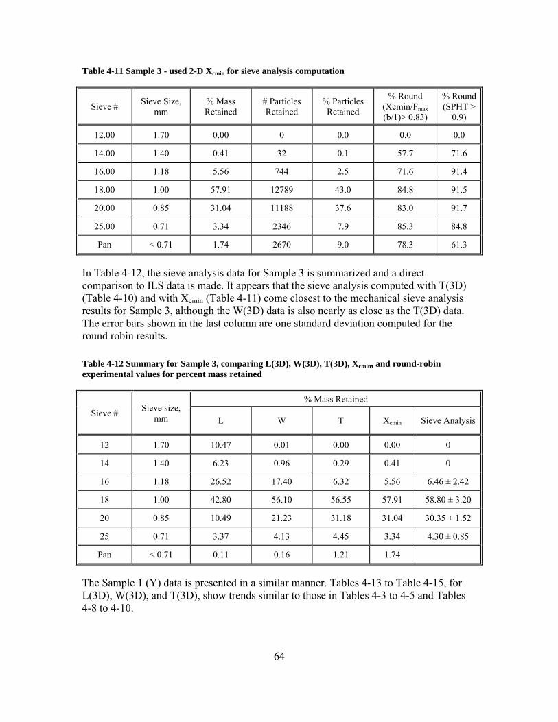
64

Table 4-11 Sample 3 - used 2-D Xcmin for sieve analysis computation

Sieve # Sieve Size,

mm % Mass Retained



% Round (Xcmin/Fmax (b/1)> 0.83)

% Round (SPHT >

0.9)

12.00 1.70 0.00 0 0.0 0.0 0.0

14.00 1.40 0.41 32 0.1 57.7 71.6

16.00 1.18 5.56 744 2.5 71.6 91.4

18.00 1.00 57.91 12789 43.0 84.8 91.5

20.00 0.85 31.04 11188 37.6 83.0 91.7

25.00 0.71 3.34 2346 7.9 85.3 84.8

Pan < 0.71 1.74 2670 9.0 78.3 61.3

In Table 4-12, the sieve analysis data for Sample 3 is summarized and a direct comparison to ILS data is made. It appears that the sieve analysis computed with T(3D) (Table 4-10) and with Xcmin (Table 4-11) come closest to the mechanical sieve analysis results for Sample 3, although the W(3D) data is also nearly as close as the T(3D) data. The error bars shown in the last column are one standard deviation computed for the round robin results.

Table 4-12 Summary for Sample 3, comparing L(3D), W(3D), T(3D), Xcmin, and round-robin experimental values for percent mass retained

Sieve # Sieve size,

mm

% Mass Retained

L W T Xcmin Sieve Analysis

12 1.70 10.47 0.01 0.00 0.00 0

14 1.40 6.23 0.96 0.29 0.41 0

16 1.18 26.52 17.40 6.32 5.56 6.46 ± 2.42

18 1.00 42.80 56.10 56.55 57.91 58.80 ± 3.20

20 0.85 10.49 21.23 31.18 31.04 30.35 ± 1.52

25 0.71 3.37 4.13 4.45 3.34 4.30 ± 0.85

Pan < 0.71 0.11 0.16 1.21 1.74

The Sample 1 (Y) data is presented in a similar manner. Tables 4-13 to Table 4-15, for L(3D), W(3D), and T(3D), show trends similar to those in Tables 4-3 to 4-5 and Tables 4-8 to 4-10.

65

Table 4-13 Sample 1 – used L (3D) length for sieve analysis computation


16 1.18 0.46 143 0.023

20 0.85 4.56 2621 0.41

30 0.60 12.41 11742 1.85

50 0.30 51.26 187911 29.59

100 0.15 31.3 430909 67.86

Pan < 0.71 0.014 1654 0.26

Table 4-14 Sample 1 – used W (3D) width for sieve analysis computation

Sieve # Sieve Size, mm % Mass Retained # Particles Retained


16 1.18 0 0 0

20 0.85 0.24 70 0.011

30 0.60 6.52 3272 0.52

50 0.30 52.78 130365 20.53

100 0.15 40.31 488019 76.86

Pan < 0.71 0.15 13254 2.09

Table 4-15 Sample 1 – used T(3D) thickness for sieve analysis computation

Sieve # Sieve Size, mm % Mass Retained # Particles Retained


16 1.18 0 0 0

20 0.85 0.005 1 0.00016

30 0.60 4.52 1945 0.31

50 0.30 49.49 102608 16.16

100 0.15 45.2 496706 78.22

Pan < 0.71 0.78 33720 5.31

66

Table 4-16, which shows the computational sieve results for Xcmin, is closest to Table 4-15, where T(3D) was used. The last two columns also contain the 2-D roundness parameters, showing the percentage of particles with values greater than the cutoff values shown. Remember that for Sample I, 70 % of the particles were designed to be round according to the roundometer. Table 4-16 shows that the apparent percentage of round particles changes with sieve size, similarly to the Sample 5 and Sample 3 results.

Table 4-16 Sample 1 – used 2-D Xcmin for sieve analysis computation

Sieve # Sieve Size,

mm % Mass Retained



% Round (Xcmin/Fmax (b/1)> 0.83)

% Round (SPHT > 0.9)

16.00 1.18 0.00 0 0.0

20.00 0.85 0.01 2 0.0 100.0 100.0

30.00 0.60 4.74 2038 0.3 60.1 69.0

50.00 0.30 48.80 98711 15.6 72.2 80.7

100.00 0.15 46.00 506370 79.8 78.5 76.7

Pan < 0.71 0.45 27859 4.4 4.0 6.6

In Table 4-17, the sieve analysis data for Sample 1 are summarized and direct comparison to the round robin average data is made. It appears that the sieve analysis computed with T(3D) (Table 4-15) and with Xcmin (Table 4-16) come closest to the mechanical sieve analysis results for Sample 1, although the W(3D) data is also nearly as close as the T(3D) data. The error bars shown in the last column are one standard deviation computed for the ILS results.

Table 4-17 Summary for Sample 1, comparing L(3D), W(3D), T(3D), Xcmin, and ILS experimental values for percent mass retained

Sieve # Sieve size,

mm

% Mass Retained

L W T Xcmin Sieve

Analysis

16.00 1.18 0.46 0.00 0.00 0.00 0.0

20.00 0.85 4.56 0.24 0.01 0.01 0.0

30.00 0.60 12.41 6.52 4.52 4.74 4.95 + 0.33

50.00 0.30 51.26 52.78 49.49 48.80 48.40 + 1.35

100.00 0.15 31.30 40.31 45.20 46.00 46.41 + 1.22

Pan < 0.71 0.01 0.15 0.78 0.45

67

4.9 Shape Results

The shape or roundness results will now be studied in more detail. The twin goals are to see if there are “best” values of the parameters that will reproduce the roundometer results, and to compare parameters against each other to see if any one is preferred. The shape parameters used in 3-D to analyze the X-ray CT data mostly involved the L(3D), W(3D), and T(3D) parameters. Note that using these three independent parameters, there are only two independent “aspect ratios” for each particle. In the section below, all three possible aspect ratios are used, defined in such a way as to be less than unity: W(3D)/L(3D), T(3D)/L(3D), and T(3D)/W(3D). Averaging over several 2-D projections, the 2-D equivalents, L(2D) and W(2D), to define W(2D)/L(2D) were computed, along with Xcmin in order to define Xcmin/L(2D), which is equivalent to the b/l parameter computed by the optical scanners in 2-D that was studied extensively in Chapter 3. All of these parameters were computed for every particle and for a varying cutoff value. That is, the mass fraction of particles with shape parameter less than or equal to a given value was computed and plotted vs. cutoff value.

An intuitive feel for how the non-roundness determinations depend on the cutoff values used can be obtained by looking at the plots of the cumulative distribution functions for each shape parameter. What will be plotted are the fraction of particles with shape parameter values less than a cutoff value (so non-round), plotted against the cutoff value. These plots must start at zero at a cutoff value of zero, and increase to unity as the cutoff value approaches the value for a sphere = 1. Figure 4-4 is for Sample 5, Figure 4-5 shows the results for Sample 3, and Figure 4-6 displays the data for Sample 1. On each graph, a horizontal line displayed represents the fraction of non-round particles as targeted for each sample. So when a distribution function crosses that horizontal line, the value of the cutoff at that point, found by dropping vertically to the x-axis, is that value that would be needed to make the fraction of non-round particles, as judged by that particular shape parameter, to be the same as that used in the sample preparation.

68

0

0.05

0.1

0.15

0.3 0.4 0.5 0.6 0.7 0.8 0.9 1

5 (C)

W/L 3DT/L 3DT/W 3DW/L 2DXcmin / L(2D)SPHT2DSPHT3D10 % line

Non

-rou

nd

mas

s fr

actio

n

Cutoff value

Figure 4-4 Showing the non-round fraction of the Sample 5 glass beads as a function of the cutoff value used, for seven different 3-D and 2-D shape parameters. The horizontal dashed line shows the 0.1 (10 %) line marking the mass fraction of non-rounds that should be contained in the sample.

0

0.05

0.1

0.15

0.2

0.25

0.3

0.4 0.5 0.6 0.7 0.8 0.9 1

3 (P)

W/L3DT/L3DT/W3DW/L2DXcmin / L(2D)SPHT2DSPHT3D20 % line

Non

-rou

nd

mas

s fr

actio

n

Cutoff value


69

0

0.05

0.1

0.15

0.2

0.25

0.3

0.35

0.4

0.4 0.5 0.6 0.7 0.8 0.9 1

1 (Y)

W/L3DT/L3DT/W3DW/L2dXcmin / L(2D)SPHT2DSPHT3D30 % line

Non

-rou

nd m

ass

frac

tion

Cutoff value


Qualitatively, considering the shapes of Figure 4-4 through Figure 4-6, it is clear that three of the shape parameters, SPHT2D, SPHT3D, and T(3D)/W(3D), are much steeper than the other four parameters near the nominal value corresponding to the percentage of non-rounds that were incorporated into the samples. This steepness means that small errors in the cutoff value used will produce large errors in the percent of non-round particles determined. That is not a good quality to have in a shape parameter. The other four shape parameters displayed in the figures: T(3D)/L(3D), W(3D)/L(3D), W(2D)/L(2D), and Xcmin/L(2D), are significantly less steep near the nominal value but there is no reason, only based on Figure 4-4 through Figure 4-6, to choose between them.

However, the parameter W(3D)/L(3D) can be eliminated based on the following single example taken from the real particles examined in the X-ray CT. Figure 4-7 shows a picture of one of the particles from the Type 5 sample. From the picture, it is quite clearly non-round. It is clear that the particle is similar to a flat disk or pie, with one wedge-shaped “piece” cut from it. Its values of L and W are therefore close to each other, giving it a value of W(3D)/L(3D) close to unity. Its actual values of L-W-T in 3-D are: 2.52-2.39-1.0. Using W/L as the determination of roundness, this ratio is 0.948. Using T(3D)/L(3D) or T(3D)/W(3D) as the roundness determinator would give 0.397 and 0.418, respectively, which would not be considered round, since the W/L cutoff for Type 5 was 0.866 (see Table 4-18). Therefore, on this basis the use of W(3D)/L(3D) is rejected, as it would improperly classify some clearly non-round particles as round.

70

Figure 4-7 A VRML image of particle number 5-b-01604 from the Sample 5 particles. The numbering system was one used internally in the X-ray CT work.

Just to make this case even more clearly, for prolate ellipsoids in 3-D, T(3D)/W(3D) should be close to one, while W(3D)/L(3D) should be less than one. For oblate ellipsoids, W(3D)/L(3D) should be close to one, while T(3D)/W(3D) or T(3D)/L(3D) should be less than one. The parameter W(3D)/L(3D) will correctly distinguish non-roundedness for the prolate case, but not for the oblate case, as is seen in Figure 4-7 above. This particle was judged to be round based on the W(3D)/L(3D) parameter. Therefore, T(3D)/L(3D) is always less than one for either prolate or oblate particles, and is the 3-D shape parameter of choice for these kinds of particles.

Three of the original seven shape parameters are still worth considering further, W(2D)/L(2D), Xcmin/L(2D), and T(3D)/L(3D). Of the two 2-D shape parameters, it has been shown before that W(2D)/L(2D) gives the intuitive aspect ratio correctly for rectangles, while Xcmin/L(2D) does not. Otherwise, they are not much different from each other. Since the glass beads in this study do not, for the most part, resemble rectangles, Xcmin/L(2D) will be considered to be the only 2-D shape parameter and T(3D)/L(3D) as the only 3-D shape parameter still to be studied.

Now that the overall appearance of the shape parameter distribution functions have been shown, the investigation can now become more quantitative to examine how the cutoff values for the various shape parameters vary and what they depend on. Table 4-18 contains the value of the cutoff that gave the exact experimental percent of non-rounds (by mass) for each sample type, using all particles found in that sample type. The experimental values come from the sample preparation as described earlier. The two shape parameters of most interest as mentioned above are shown in bold in Tables 4-18 and 4-19.

71

Table 4-18 Roundness cutoffs using various parameters

5 (C, 10 % non‐rounds) 3 (P, 20 % non‐rounds) 1 (Y, 30 % non‐rounds)

Parameter Cutoff value Parameter Cutoff value Parameter Cutoff value

W(3D)/L(3D) 0.858 W(3D)/L(3D) 0.896 W(3D)/L(3D) 0.895

T(3D)/L(3D) 0.796 T(3D)/L(3D) 0.838 T(3D)/L(3D) 0.819

T(3D)/W(3D) 0.928 T(3D)/W(3D) 0.937 T(3D)/W(3D) 0.948

SPHT3D 0.842 SPHT3D 0.839 SPHT3D 0.818

W(2D)/L(2D) 0.866 W(2D)/L(2D) 0.899 W(2D)/L(2D) 0.885

Xcmin/L(2D) 0.848 Xcmin/L(2D) 0.871 Xcmin/L(2D) 0.852

SPHT2D 0.935 SPHT2D 0.937 SPHT2D 0.918

Note that in Table 4-18 there are different values of the cutoff value for each sample type (size class) and each shape parameter. Based on the target roundness of the three glass bead types, it is clear that using a nominal cutoff value of 0.83 for the Xcmin/L (2D) parameter will not give correct results.

By taking the range found for the cutoff values for each roundness parameter, the range of non-round fractions that would have been found using this range of cutoff values can be computed. This is an illustration of the sensitivity in the non-roundness computed fraction to the actual cutoff value used. For example, for the T(3D)/L(3D) shape parameter, the cutoff values that gave the correct results for each sample were 0.796, 0.838, and 0.8185 or a range of 0.796 – 0.838. So the percent of non-rounds were computed for each sample using all three values, giving a range of results. Results for all the samples and all seven shape parameters are shown in Table 4-19.

72

Table 4-19 For each roundness parameter, the range found over the three sample types is shown, as well as the range of non-round fractions that would be obtained using this range

Roundness Parameter

Range of Cutoff Values

Non‐Round Fractions

Sample 5 (C) Sample 3 (P) Sample 1 (Y)

W(3D)/L(3D) 0.8575 – 0.8955 0.0999 – 0.1173 0.1777 – 0.2002 0.256 – 0.3006

T(3D)/L(3D) 0.796 – 0.838 0.100 – 0.1136 0.1763 – 0.2003 0.2787 – 0.3216

T(3D)/W(3D) 0.928 – 0.9475 0.09945 – 0.1922 0.1547 – 0.2874 0.2105 – 0.2994

SPHT3D 0.818 – 0.842 0.062 – 0.100 0.130 – 0.217 0.299 – 0.406

W(2D)/L(2D) 0.866 – 0.899 0.1000 – 0.1137 0.1738 – 0.2005 0.2762 – 0.3231

Xcmin/L(2D) 0.8475 – 0.8705 0.1001 – 0.1105 0.1772 – 0.1999 0.2931 – 0.3446

SPHT2D 0.918 – 0.937 0.0727 – 0.1059 0.1298 – 0.1990 0.3007 – 0.4085

The results listed in Table 4-18 and Table 4-19 clearly imply that there is no one value of the cutoff for T(3D)/L(3D) or for Xcmin/L(2D) that will give the correct value of non-roundness for all three different size classes. However, suppose one was forced to estimate what the “best” value of a constant would be, which minimized the total error across the three samples for Xcmin/L(2D). If one minimized the sum of the errors in each of the three samples, one would get 0.8556, which gives an error of 3.8 % for Sample 5 (C), an error of -7.4 % for Sample 3 (P), and an error of 3.7 % for Sample 1 (Y). These errors are calculated assuming that the experimental results are exact. If these errors are acceptable, one might be able to recommend this cutoff value for the Xcmin/L(2D) parameter. But this cutoff value really does depend on particle size, as will be shown more clearly later in this report. The same calculation done for the T(3D)/L(3D) parameter would give 0.8160, which gives an error of 6.5 % for Sample 5 (C), an error of -6.1 % for Sample 3 (P), and an error of -0.3 % for Sample 1 (Y).

Figure 4-8 through Figure 4-10 below show how Xcmin/L(2D) and T(3D)/L(3D) relate for the particles tested in the X-ray CT scans by plotting the 2-D parameter against the 3-D parameter. In this way of plotting the data, we are thinking of the 3-D parameter as being correct, and seeing how well the 2-D parameter can predict its value. This kind of graphical analysis will better show how the 2-D and 3-D parameters relate. A line has been fit through each cloud of points, which has a slope of well less than one. However, the fitted slopes and intercepts are fairly consistent for all three samples. One can understand why Xcmin/L(2D) is usually greater than T(3D)/L(3D) especially at lower values by considering a single example. Consider a prolate ellipsoid in 3D with L = 10, and T = W = 1. Then T(3D)/L(3D) = 0.1. However, if a 2-D projection was taken along the long axis, then Xcmin/L(2D) = 1, which would make the average over several views be greater than 0.1.

73

0.2

0.3

0.4

0.5

0.6

0.7

0.8

0.9

1

0.2 0.3 0.4 0.5 0.6 0.7 0.8 0.9 1

1 (Y)

y = 0.33088 + 0.62261x R= 0.93962

Xcm

in /

L(2

D)

T(3D) / L(3D)

Figure 4-8 Xcmin/L(2D) plotted vs. T(3D)/L(3D), for Sample 1 particles.

0.2

0.3

0.4

0.5

0.6

0.7

0.8

0.9

1

0.2 0.3 0.4 0.5 0.6 0.7 0.8 0.9 1

3 (P)

y = 0.28233 + 0.68637x R= 0.97059

Xcm

in /

L(2

D)

T(3D) / L(3D)

Figure 4-9 Xcmin/L(2D) plotted vs. T(3D)/L(3D), for Sample 3 particles

74

0.2

0.3

0.4

0.5

0.6

0.7

0.8

0.9

1

0.2 0.3 0.4 0.5 0.6 0.7 0.8 0.9 1

5 (C)

y = 0.2733 + 0.69931x R= 0.97653

Xcm

in /

L(2

D)

T(3D) / L(3D)

Figure 4-10 Xcmin/L(2D) plotted vs. T(3D)/L(3D), for Sample 5 particles

To investigate the robustness of the Xcmin/L(2D) shape parameter, it is informative to compare the results for the Sample 1 particles vs. a sample that was totally made up of particles that had been declared to be “non-round” by the mechanical roundometer. The average particle size was similar, roughly 0.3 mm. The sample that was made up of these particles was denoted Sample A. An X-ray CT sample was made for the Sample A particles, similar to those used for the other samples. A total of 5217 particles (1.2 g) were extracted from the X-ray CT images. The ratio Xcmin/L(2D) was calculated.

In Figure 4-11 below, the mass fraction of particles with Xcmin/L(2D) less than a cutoff value was plotted vs. the cutoff value for Sample A and for the Sample 1 (Y) particles. The two sets of particles are enormously different in terms of shape as measured by the 2-D parameter Xcmin/L(2D). The vertical dashed line is drawn at a cutoff value of 0.83, the nominal value used in the optical studies. The intersection of this line with the two curves shows that fraction of particles with values of Xcmin/L(2D) less than 0.83: about 0.25 for the Sample 1 (Y) particles and about 0.80 for the Sample A particles. The horizontal line is drawn at 0.3, since Sample 1 was designed to contain 30 %, by mass, of particles that were judged to be non-round by the Roundometer. The cutoff value at which the Sample 1 particles achieve 30 % is at about 0.85, while the Sample A particles achieve 30 % non-round with respect to this parameter at a cutoff value of about 0.66. Clearly the Sample A particles are much more “non-round” than are the Sample 1 (Y) particles, as the case should be, and the parameter Xcmin/L(2D) clearly shows that difference.

75

0

0.2

0.4

0.6

0.8

1

0.4 0.5 0.6 0.7 0.8 0.9 1

Sample ASample 1 (Y)0.83 line30 % line

Non

-rou

nd

mas

s fr

actio

n

Cutoff value

Figure 4-11 Showing the non-round mass fraction of the Sample 1 (Y) glass beads and the Sample A glass beads, as a function of the cutoff value used, using the 2-D shape parameter Xcmin/L(2D). The horizontal dashed line shows the 0.3 (30 %) line marking the mass percent of non-rounds that should be contained in the sample, as determined by the roundometer and sample preparation. The vertical dashed line is drawn at a cutoff value of 0.83, which was used in the round robin optical scanning results.

4.10 Dependence of Roundness Cutoff on Particle Size (Sieve Class)

When discussing Table 4-6, Table 4-11, and Table 4-16, it was mentioned that the computed results for Xcmin/L(2d) appeared to depend on sieve number (particle size). The ILS experimental data also shows this behavior. Therefore, it was of interest to compute the non-round mass fraction for the X-ray CT data for different sieve classes. For each sample type, two sieve size classes were chosen, the two that contained most of the particles. The mass fraction of non-rounds was computed for various values of the cutoff in terms of Xcmin/L(2D), and the results plotted below, in a format similar to that of Figure 4-4 through Figure 4-6.

76

0

0.1

0.2

0.3

0.4

0.5

0.6

0.6 0.65 0.7 0.75 0.8 0.85 0.9 0.95 1

5 (C)

AllRetained on #14Retained on #1610 % line

Non

-rou

nd

mas

s fr

actio

n

Cutoff value

Figure 4-12 Showing the mass fraction of non-rounds vs. the cutoff value used to define the mass fraction, for the Sample 5 particles. The non-round data is computed separately for particles retained on the #14 sieve, the #16 sieve, and all the particles averaged together.

0

0.1

0.2

0.3

0.4

0.5

0.6

0.6 0.65 0.7 0.75 0.8 0.85 0.9 0.95 1

3 (P)


Non

-rou

nd m

ass

frac

tion

Cutoff value


77

0

0.1

0.2

0.3

0.4

0.5

0.6

0.6 0.65 0.7 0.75 0.8 0.85 0.9 0.95 1

1 (Y)


Non

-rou

nd

mas

s fr

actio

n

Cutoff value


Figure 4-12 through Figure 4-14 clearly show that there is not only variation in the cutoff value that makes the 2-D results agree with the roundometer, but that there is also some degree of variation in the shape of the curves. This is an interesting result that might indicate some processes (e.g. melting together, chipping) at work that act to make non-round particles more or less common at different size classes.

4.11 Further Comparison of 2-D vs. 3-D Shape Parameters

Another way to compare 2-D to true 3-D results, round or non-round, is to look at how the Volume Equivalent Spherical Diameter (VESD) in 2-D compares to the VESD in 3-D. The VESD is the diameter of the sphere (circle) with equivalent volume (area) to the real particle. For a perfect sphere, its 2-D projection is a circle with the same radius and so the 2-D VESD would be the same as the 3-D VESD. For non-round particles, this is no longer true. In the following, the VESD (2D) is plotted against the VESD (3D) for round and non-round particles, as determined by either T(3D)/L(3D) or Xcmin/L(2D), to see how effective these two parameters are at discriminating between round and non-round particles. The idea is that the particles considered to be round should have VESD values in 2-D and 3-D that are nearly equal, while a greater difference between 2-D and 3-D should be seen for the non-round particles, since the VESD values are only truly equivalent in 2-D and 3-D for spherical particles.

78

0.5

1

1.5

2

2.5

0.5 1 1.5 2 2.5

Sample 5 (C) T(3D)/L(3D) NRy = -0.025089 + 0.95611x R= 0.99804

VE

SD

(2D

, m

m)

VESD (3D, mm)

Figure 4-15 Showing VESD (2D) vs. VESD (3D) for the Sample 5 particles, for the 10 % by mass that were judged to be non-round by the T(3D)/L(3D) shape parameter. The dashed line is fit through the points; the dotted line is the line of equality.

0.5

1

1.5

2

2.5

0.5 1 1.5 2 2.5

Sample 5 (C) NR Xcmin/L(2D)

y = -0.024792 + 0.95576x R= 0.99808

VE

SD

(2D

, m

m)

VESD (3D, mm)

Figure 4-16 Showing VESD (2D) vs. VESD (3D) for the Sample 5 particles, for the 10 % by mass that were judged to be non-round by the Xcmin/L(2D) shape parameter. The dashed line is fit through the points; the dotted line is the line of equality.

79

Note that Figure 4-15 and Figure 4-16 are for Sample 5, where only the 10 % of the particles were used that were judged to be non-round by T(3D)/L(3D) (Figure 4-15) and Xcmin/L(2D) (Figure 4-16). The two figures are almost identical, with practically the same slope on the fitted line, which implies that T(3D)/L(3D) and Xcmin/L(2D) are measuring practically the same thing, but with slightly different numerical values.

0.5

1

1.5

2

2.5

0.5 1 1.5 2 2.5

Sample 5 (C) Round T(3D)/L(3D)

y = -0.059755 + 1.0154x R= 0.99963

VE

SD

(2

D. m

m)

VESD (3D, mm)

Figure 4-17 Showing VESD (2D) vs. VESD (3D) for the Sample 5 particles, for the 90 % by mass that were judged to be round by the T(3D)/L(3D) shape parameter. The dashed line is fit through the points; the dotted line is the line of equality.

80

0.5

1

1.5

2

2.5

0.5 1 1.5 2 2.5

Sample 5 (C) Round Xcmin/L(2D)

y = -0.059558 + 1.0153x R= 0.99964

VE

SD

(2D

, mm

)

VESD (3D, mm)

Figure 4-18 Showing VESD (2D) vs. VESD (3D) for the Sample 5 particles, for the 90 % by mass that were judged to be round by the Xcmin/L(2D) shape parameter. The dashed line is fit through the points; the dotted line is the line of equality.

Note that Figure 4-17 and Figure 4-18 are for Sample 5, where now the 90 % of the particles were used that were judged to be round by T(3D)/L(3D) (Figure 4-17) and Xcmin/L(2D) (Figure 4-18). The two figures are almost identical, with practically the same slope on the fitted line, which implies that T(3D)/L(3D) and Xcmin/L(2D) are measuring practically the same thing, but with slightly different numerical values. Also, the data falls much closer to the line of equality, which is another indication that the particles are more spherical.

81

0.6

0.8

1

1.2

1.4

1.6

1.8

2

2.2

0.6 0.8 1 1.2 1.4 1.6 1.8 2 2.2

Sample 3 (P) Nonround T(3D)/L(3D)

y = 0.031124 + 0.9203x R= 0.99244

VE

SD

(2D

, mm

)

VESD (3D, mm)

Figure 4-19 Showing VESD (2D) vs. VESD (3D) for the Sample 3 particles, for the 20 % by mass that were judged to be non-round by the T(3D)/L(3D) shape parameter. The dashed line is fit through the points; the dotted line is the line of equality.

82

0.6

0.8

1

1.2

1.4

1.6

1.8

2

2.2

0.6 0.8 1 1.2 1.4 1.6 1.8 2 2.2

Sample 3 (P) Nonround (Xcmin/L 2D)

y = 0.014633 + 0.9322x R= 0.99458

VE

SD

(2D

, mm

)

VESD (3D, mm)


Note that Figure 4-19 and Figure 4-20 are for Sample 3, where only the 20 % of the particles were used that were judged to be non-round by T(3D)/L(3D) (Figure 4-19) and Xcmin/L(2D) (Figure 4-20). The two figures are almost identical, with practically the same slope on the fitted line, which implies that T(3D)/L(3D) and Xcmin/L(2D) are measuring practically the same thing, but with slightly different numerical values.

83

0.6

0.8

1

1.2

1.4

1.6

1.8

2

2.2

0.6 0.8 1 1.2 1.4 1.6 1.8 2 2.2

Sample 3 (P) Round T(3D)/L(3D)

y = -0.054352 + 1.0219x R= 0.99938

VE

SD

(2D

, mm

)

VESD (3D, mm)

Figure 4-21 Showing VESD (2D) vs. VESD (3D) for the Sample 3 particles, for the 80 % by mass that were judged to be round by the T(3D)/L(3D) shape parameter. The dashed line is fit through the points; the dotted line is the line of equality.

0.6

0.8

1

1.2

1.4

1.6

1.8

2

2.2

0.6 0.8 1 1.2 1.4 1.6 1.8 2 2.2

Sample 3 (P) Round (Xcmin/L 2D)

y = -0.050675 + 1.0185x R= 0.99941

VE

SD

(2D

, mm

)

VESD (3D, mm)


84

Note that Figure 4-21 and Figure 4-22 are for Sample 3, where now the 80 % of the particles were used that were judged to be round by T(3D)/L(3D) (Figure 4-21) and Xcmin/L(2D) (Figure 4-22). The two figures are almost identical, with practically the same slope on the fitted line, which implies that T(3D)/L(3D) and Xcmin/L(2D) are measuring practically the same thing, but with slightly different numerical values. Also, the data falls much closer to the line of equality, which is another indication that the particles are more spherical.

Figure 4-23 is for Sample 1, where the 30 % of the particles were used that were judged to be non-round by Xcmin/L(2D). The equivalent figure using T(3D)/L(3D) is omitted – it was very similar.

0.1

0.2

0.3

0.4

0.5

0.6

0.7

0.8

0.9

0.1 0.2 0.3 0.4 0.5 0.6 0.7 0.8 0.9

Sample 1 (Y) Nonround Xcmin/L(2D)

y = -0.0071727 + 0.95297x R= 0.99796

VE

SD

(2D

, m

m)

VESD (3D, mm)


85

0.1

0.2

0.3

0.4

0.5

0.6

0.7

0.8

0.1 0.2 0.3 0.4 0.5 0.6 0.7 0.8

Sample 1 (Y) Round Xcmin/L(2D)

y = -0.01407 + 1.0124x R= 0.99966

VE

SD

(2D

, m

m)

VESD (3D, mm)


Figure 4-24 is for Sample 1, where 70 % of the particles by mass were used that were judged to be round by Xcmin/L(2D). The equivalent figure using T(3D)/L(3d) is omitted – it was very similar. Clearly the data falls much closer to the line of equality than in Figure 4-23, which is another indication that the particles are more spherical.

A final way to link 2-D quantities with 3-D quantities is to compare the sphericity parameter, Eqs. (2) and (6), as defined in 2-D and 3-D, for the same particles. This can be done since the X-ray CT and spherical harmonic analysis computes both 2-D and 3-D parameters on the same particle. These were compared for all the particles, not the round and non-round (as judged by some shape parameter) separately.

86

0.5

0.6

0.7

0.8

0.9

1

0.5 0.6 0.7 0.8 0.9 1

Sample 1 (Y)

SP

HT

2D

SPHT3D

Figure 4-25 Showing the 2-D sphericity vs. the 3-D sphericity for Sample 1. Only a random 1 % of the possible data points are shown.

Figure 4-25 shows the 2-D sphericity vs. the 3-D sphericity for Sample 1. As indicated from the figure, the 2-D values are slightly overestimated, since the perimeter correction made, a multiplication of the pixel perimeter by a factor of /4, will tend to make the perimeter too small and hence the 2-D sphericity too large. This is not a large error, 5 % at the most, as the largest 2-D sphericity was only 1.05, instead of having one as a maximum value. Therefore, Figure 4-25 clearly shows, for the Sample 1 (Y) particles, that the 2-D values of sphericity, as optically measured, tend to overestimate the actual 3-D sphericity. The average of (2D-3D)/3D = 14 % + 6 %. Even if the 2-D values were to be dropped by 5 %, as indicated above, it would still mean on average, the 2-D sphericity overestimates the 3-D value by about 10 % and this overestimation can be more. Figure 4-26 and Figure 4-27 show similar results for Samples 3 and 5, again with only some of the points shown. The results are similar to those for Sample 1. All three figures are showing that the SPHT2D and SPHT3D parameters, although both are defined as sphericities, are not measuring the same thing because of the non-round particles present and because of the difference in dimensionality.

87

0.5

0.6

0.7

0.8

0.9

1

0.5 0.6 0.7 0.8 0.9 1

Sample 3 (P)

SP

HT

2D

SPHT3D

Figure 4-26 Showing the 2-D sphericity vs. the 3-D sphericity for Sample 3. Only a random fraction of the possible data points are shown.

0.5

0.6

0.7

0.8

0.9

1

0.5 0.6 0.7 0.8 0.9 1

Sample 5 (C)

SP

HT

2D

SPHT3D

Figure 4-27 Showing the 2-D sphericity vs. the 3-D sphericity for Sample 5. Only a random fraction of the possible data points are shown.

88

4.12 Images of Non-Round Particles for Different Samples

For each sample (1, 3, 5, and A), images of a few non-round particles have been selected in order to qualitatively illustrate the range of non-round particles that can be encountered. For each sample, a table gives the approximate particle size in terms of the VESD, and the shape in terms of several shape parameters. The number label for each particle is from an internal numbering system for the X-ray CT data, and has no special significance. The images are approximately to the same scale, but magnified for easier viewing.

Table 4-20 shows the properties of four non-round particles from Sample 2 pictured in Figure 4-28. Sample A was the sample of particles that were all judged to be non-round by roundometer results.

Table 4-20 For Sample A, the geometric details for four typical particles, pictured in Figure 4-28.

Bead # VESD (mm) SPHT3D T(3D)/L(3d)

1 0.336 0.83 0.46

3 0.253 0.77 0.68

20 0.255 0.85 0.71

87 0.289 0.70 0.43

Figure 4-28 Showing four typical particles from Sample A. Their geometrical parameters are listed in Table 4-20.

Sample 1 contained the smallest particles, where 30 % of the particles by mass were judged to be non-round by the roundometer. Note that particle no. 14526 in Table 4-21 and Figure 4-29 is probably a real double particle, and not an artificially touching particle in the image analysis of the X-ray CT results.

89

Table 4-21 Sample 1 “non-round” particles – three with Xcmin/L(2D) < 0.475, and four with Xcmin/L(2D) = 0.600

Bead # VESD (mm) SPHT3D Xcmin/L(2D) T(3D)/L(3D)

37 0.163 0.62 0.454 0.35

13601 0.113 0.50 0.446 0.27

31891 0.159 0.53 0.470 0.27

9633 0.117 0.64 0.600 0.42

14526 0.421 0.71 0.600 0.51

29021 0.246 0.68 0.600 0.54

50211 0.204 0.64 0.600 0.41

90

Figure 4-29 Typical non-round particles in Sample 1. Geometrical details are in Table 4-21.

Table 4-22 Sample 3 “non-round” particles – one with Xcmin/L(2D) < 0.475, and four with Xcmin/L(2D) = 0.600. “3a” and “3b” are internal labels indicating from which of the five Type 3 sub-samples these images were taken.

Bead # VESD (mm) SPHT3D Xcmin/L(2D) T(3D)/L(3D)

253 1.420 0.71 0.472 0.42

53 1.110 0.78 0.600 0.44

1182 1.110 0.77 0.601 0.52

3169 1.210 0.78 0.600 0.52

4450 0.810 0.69 0.600 0.56

91

Figure 4-30 Typical non-round particles in Sample 3. Geometrical details are given in Table 4-22.

Table 4-22 Sample 5 “non-round” particles – one with Xcmin/L(2D) < 0.475, and five with Xcmin/L(2D) = 0.600. The particles are shown in Figure 4-31.

Bead # VESD (mm) SPHT3D SPHT2D Xcmin/L(2D) T(3D)/L(3D)

1582 2.25 0.65 0.71 0.44 0.31

2421 1.98 0.87 0.99 0.69 0.57

57 1.79 0.88 0.96 0.62 0.50

2 1.74 0.85 0.89 0.69 0.61

616 1.04 0.81 0.82 0.70 0.59

427 2.10 0.77 0.84 0.61 0.55

92

Figure 4-31 Some typical non-round particles in Sample 5. Geometrical details are in Table 4-23.

93

CHAPTER 5- CONCLUSIONS AND RECOMMENDATIONS

5.1 Conclusions

Manufacturers of computerized optical equipment have developed various applications for the analysis of glass beads used in traffic markings. However, there are no standard test methods to be followed for the use of this equipment. Furthermore, the precision and bias of the computerized methods, and how they are compared with the precision and bias of the current manual ASTM methods, are not known. This study involved design and conduct of an interlaboratory study to determine the precision and bias of both optical and traditional methods, to make a comparison of the precision and bias of various measurement methods, and to develop a test method for use with the computerized method that is provided in Appendix H. An important part of the study was to validate the collected optical data using an independent analysis in 3-D of glass bead size and shape distribution using X-ray microtomography.

Three methods were used in this study for each size and roundness measurements: two computerized optical methods (COM-A and COM-B) and the traditional mechanical methods (sieving, roundometer) following ASTM C 1139 and ASTM C 1048. The most number of datasets were provided using mechanical sieving and the roundometer, which included 14 sets of size distribution and 11 sets of roundness data. COM-A users provided 8 sets of data, which included both size and roundness data. COM-B data were received from 4 laboratories on small size glass beads (Type 1) and from only one laboratory on larger glass beads (Types 3 and 5). Recall that the samples upon which these tests were run were carefully prepared via mechanical sieving and mechanical roundness measurement, so “accuracy” in the ILS for the roundometer, COM-A, COM-B, and X-ray tomography results means how close did these measurement methods come to the original mechanical sieving and roundness measurements, allowing for some uncertainty to be introduced in the sample preparation process.

The interlaboratory study data that were received from participating laboratories were statistically analyzed for accuracy and precision. The significance of the bias for each method between measured and target values were evaluated separately for each sieve size of each glass type using the Student t-test. Following the ASTM E 691 methodology, both within and between laboratory variability of the computerized and mechanical methods was also determined for each sieve size of each glass bead type.

The computed t values and the computed within- and between- laboratory standard deviations for each glass bead type were compared to examine the accuracy and precision of the different methods in measuring the properties of the glass beads. For each glass bead type, comparison was made between the statistics corresponding to the sieve sizes retaining the highest mass percentage of the beads. This was because these sieves

94

provided more precise measurements of the glass bead type.

Since only one laboratory provided size and roundness measurements of Type 3 and 5 glass beads using the COM-B instrument, the discussion of precision and bias for measuring properties of Type 3 and Type 5 glass beads does not involve the COM-B results. The results of the comparison are summarized as follows:

Mechanical sieving, the COM-A device, and the COM-B instrument were used for measuring the size of Type 1 glass beads. Analysis of the mass percent retained in the largest size class of the Type 1 samples indicated that among the three methods of measurements, the COM-B device provided the most accurate measurement of the size of Type 1 glass beads. With respect to variability, the mechanical sieve provided the smallest within-laboratory standard deviation for measuring the size of the small beads. However, the between- laboratory precisions of the three methods were very similar.

Data from mechanical sieving and the COM-A device were used to develop precision and bias assessments for size measurement of the Type 3 and Type 5 beads. Between the two methods, the COM-A instrument measured the size of the Type 3 and Type 5 glass beads with more accuracy than the mechanical sieves. In addition, the COM-A device provided smaller within- and between-laboratory variability than did the mechanical sieves.

A combination of four methods/parameters was used for measuring the roundness of Type 1 glass beads: the mechanical roundometer, the COM-A b/l and SPHT parameters, and the COM-B T/L parameter. Among the four methods/parameters, the COM-B parameter provided the most accurate measurement of roundness of small glass beads. However, the COM-A b/l parameter provided the most precise within- and between-laboratory measurements. The mechanical roundometer did not provide equivalent accuracy and precision for measuring the roundness of Type 1 glass beads.

A combination of three methods/parameters was used for measuring the roundness of Type 3 and Type 5 glass beads: the mechanical roundometer and the COM-A b/l and SPHT parameters. Among the three methods/parameters, the COM-A b/l parameter provided the most accurate and precise measurement of the roundness of Type 3 and Type 5 glass beads. The mechanical roundometer did not provide equivalent accuracy and precision in measuring the mass percent round of Type 3 and Type 5 glass beads.

From analysis of the results of the interlaboratory study, it can be concluded that computerized optical methods are preferred over the traditional mechanical methods for measuring the size and roundness of glass beads. The improved statistics of the b/l parameter for the larger glass beads indicated the advantage of COM-A over the roundometer for roundness measurement of the larger glass beads. Although a smaller number of laboratories provided data using the COM-B device, both size and roundness

95

of the Type 1 glass beads were correctly measured by the COM-B instrument.

The following are results of 2-D and 3-D analysis of the X-ray microtomography data:

Of the three 2-D shape parameters considered, Xcmin/L(2D), which is equivalent to b/l, works well for predicting the mechanical roundness analysis and seems to be adequate for making distinctions between round and non-round particles, as judged by the roundometer. However, this is only true because the majority of the glass beads is mainly near-spherical particles, and if the roundness cutoff value is adjusted as recommended below.

A single cutoff value for the Xcmin/L(2D) parameter is not adequate to classify all the glass beads into round and non-round categories. Rather, the cutoff value seems to depend on particle size as determined by the different sieve classes.

In general, the values of 2-D and 3-D shape parameters are not analytically related for the glass bead particles. However, there are reasonable empirical correlations between them that are obviously useful.

5.2 Recommendations

A ruggedness study for the developed computerized optical test method seems necessary. This would detect the parameters of the test procedure that cause significant variability in the test results and determine the controls necessary for the parameters in the test method. For example, the effect of image analysis threshold value on the size distribution should be evaluated for the optical measurements. The number and direction of images taken from falling particles on the correlation of 2-D and 3-D measurements is another factor that should be examined.

Since there is an effect of particle size on the shape parameter cutoff value, there is a need to use the results of this report or perhaps the results of a further study to make better recommendations for how to use 2-D optical scanning results in glass bead roundness classification. The approximately 700 000 particles in the X-ray CT and spherical harmonic database can be used to analyze any new results, and the techniques are in place to generate new X-ray CT data as needed. This database can certainly be mined further.

The results of the ILS and analysis of X-ray images implied that the existing cutoff values for the 2-D roundness parameters were not large enough for detecting the intended roundness of the prepared glass beads. This was clearly shown by the overestimation of the roundness of the ILS samples by participating laboratories and from the comparison of 2-D with 3-D roundness results of X-ray images of the glass beads. Based on the results of the shape analysis in Chapter 4, it is recommended that the threshold value of b/l parameter to be increased from 0.83 to 0.85 and that of the SPHT parameter to be increased from 0.90 to 0.93. The threshold value of 0.83 was found to be adequate for

96

T/L parameter.

What is the glass bead shape that is actually needed to have good retroreflectivity? It seems intuitively clear that spheres are best, but how much and what kind of non-roundness can be tolerated? Having such a physical criteria would help move the community beyond the roundometer results and allow a true performance-based glass bead specification to be formulated and issued. This question can be addressed through direct computation of light reflection on X-ray CT spherical harmonic images [23].

Using a computational technique like Discrete Element Mechanics (DEM), the actual dynamics of the roundometer could be simulated, using the same particles that were imaged in the X-ray CT and their geometric shape determined directly. That way the shapes that are judged to be non-round and round by the roundometer would be known exactly. This would lend an element of increased accuracy to the roundometer, which would strengthen any new optical light-reflection results.

97

REFERENCES

1. AASHTO Standard Specifications for Transportation Materials and Methods of Sampling and Testing (Part 1 – Specifications), Twenty-Ninth Edition, American Association of State Highway and Transportation Officials, Washington, DC. 2009.

2. ASTM Book of Standards, ASTM D1214 - 04 Standard Test Method for Sieve Analysis of Glass Spheres, Vol. 06.02, Paint and Related Coating Standards, West Conshohocken, PA, 2009.

3. ASTM Book of Standards, ASTM D1155 - 03 Standard Test Method for Roundness of Glass Spheres Vol. 06.02, Paint and Related Coating Standards, West Conshohocken, PA, 2009.

4. ASTM Book of Standards, E691 - 09 Standard Practice for Conducting an Interlaboratory Study to Determine the Precision of a Test Method, Vol. 14.02, Quality Control Standards, West Conshohocken, PA, 2009.

5. E.E. Underwood, 1970. Quantitative Stereology. Addison-Wesley.

6. B. Mather, (1966) “Shape, Surface Texture and Coatings”. ASTM STP 169A Significance of Tests and Properties of Concrete and Concrete Making Materials (American Society for Testing and Materials (ASTM), Philadelphia 1966), p. 571.

7. J.C. Russ, The Image Processing Handbook (5th edition) (Boca Raton, CRC Press, 2007).

8. A.C. Kak and M. Slaney, Principles of Computerized Tomographic Imaging (SIAM, New York, 2001).

9. M.A. Taylor, E.J. Garboczi, S.T. Erdoğan, and D.W. Fowler, Some properties of irregular particles in 3-D, Powder Technology 162, 1-15 (2006).

10. E.J. Garboczi, Three-dimensional mathematical analysis of particle shape using X-ray tomography and spherical harmonics: Application to aggregates used in concrete, Cem. Conc. Res. 32, 1621-1638 (2002).

11. S.T. Erdoğan et al., Three-dimensional shape analysis of coarse aggregates: New techniques for and preliminary results on several different coarse aggregates and reference rocks, Cem. Conc. Res. 36, 1619-1627 (2006).

12. M. Grigoriu, E.J. Garboczi, and C. Kafali, Spherical harmonic-based random fields for aggregates used in concrete, Powder Technology 166, 123-138 (2006).

13. G. Arfken, Mathematical Methods for Physicists (Academic Press, New York,

98

1970).

14. D.F. Lawden, D.F. (1989) Elliptic Functions and Applications (Springer-Verlag, Berlin, 1989).

15. A.-M. Legendre, (1825) Traite des Fonctions Élliptiques, tome 1 (Huzard-Courchier, Paris, 1825).

16. L.R.M. Maas, (1994), “On the surface area of an ellipsoid and related integrals of elliptic integrals,” J. Comp. Appl. Math. 51, 237-249. Note that Maas’ formula for the ellipsoid surface area has an incorrect prefactor for the term involving the elliptic E function of the second kind. Lawden’s reference has the correct prefactor.

17. Numericana - http://home.att.net/~numericana/answer/ellipse.htm#pade

18. H. Azari and E.J. Garboczi, companion TRB paper to this report, in preparation.

19. E.J. Garboczi and P.T. Metzger, Three Dimensional Shape Analysis of Simulated Lunar Soil Particles, in preparation.

20. N.S. Martys and E.J. Garboczi, “Length scales relating fluid permeability and electrical conductivity in model 2-D porous media,” Physical Review B 46, 6080-6090 (1992).

21. J.M.R. Fernlund, The Effect of Particle Form on Sieve Analysis: A Test by Image Analysis, Engineering Geology 50 (1), September 1998, pp. 111-124.

22. S.T. Erdogan, D.W. Fowler, and E.J. Garboczi, Shape and size of microfine aggregates: X-ray microcomputed tomography vs. laser diffraction, Powder Technology 177, 53-63 (2007).

23. M.I. Mishchenko, J.W. Hovenier, and L.D. Travis (eds.), Light Scattering by Non-Spherical Particles (Academic Press, San Diego, 2000).

99

APPENDIX A—INSTRUCTIONS AND DATA SHEET FOR INTERLABORATORY STUDY

100

Instructions to the Laboratories Participating in the AASHTO Interlaboratory Study for Development of Test Method for Optical Sizing and Roundness Determination of Glass Beads Utilized in Traffic Markings

Dear participating laboratories, you should have received the following glass bead samples:

o Y010-a, Y010-b, and Y010-c

o Y020-a, Y020-b, and Y020-c

o P020-a, P020-b, and P020-c

o C020-a, C020-b, and C020-c

Please follow the instructions below for testing the beads.

Instructions for using ASTM Sieve Analysis Method

Tare a 600 ml beaker.

Pour the entire content of one bottle into the beaker.

Record the sample weight.

Place the beaker in an 110C ± 5C oven for one hour to dry them out.

Let the beads cool to room temperature for 15 min before sieving.

For the beads labeled as Y series use #16, #20, #30, #50, and #100 sieve sizes.

For the beads labeled as P series use #12, #14, #16, #18, #20, and #25 sieve sizes.

For the beads labeled as C series use #8, #10, #12, #14, #16, and #18 sieve sizes.

Follow the instructions in Section 7.1.2 through 7.1.5 of ASTM D 1214 to hand sieve the beads or follow Section 7.2 to machine sieve the beads. Record all the weights to the nearest 0.01 g instead of 0.1g.

Report the following information:

o Weight of materials retained on each sieve to the nearest 0.01 g.

o Percent passing each sieve, expressed to the nearest 0.1 %.

101

o The method of sieving used.

Email the results to [email protected].

Instructions for Using ASTM Round‐O‐Meter


Pour glass beads of one size class from previous section into the beaker.

Record the sample weight to the nearest 0.01 g.

If it is humid, place the beaker of sieved beads in the drying oven at 110C ± 5C for one hour to dry them out.

Clean the inclined glass surface plate of the round-o-meter by wiping it with 2-propanol.

Using a digital level, approximately 12-24 inches long, set the plate angle as follows:

o 1.0 for testing #20 and larger glass beads.

o 1.1 for testing # 30 glass beads.

o 2.3 for # 50 glass beads.

o 3.9 for # 100 glass beads.

Pour the beads slowly from a height of ½ in. to a point in the center of the plate 1/3 down from the uphill end.

Turn on the switch to start the plate vibrator and follow Section 8.3 through 8.6 of ASTM D1155.

When each size class has been separated, pour the beads from each pan into separate beakers. You will end up with two beakers for each sieve size.

When all the size classes have been separated, weigh the rounds and non rounds in each size group to the nearest 0.01 g. (Weigh the beaker+ beads, and then subtract the beaker weight).

Record the weights to the nearest 0.01 g. Calculate the percent rounds and nonrounds in each size group to the nearest 0.1 %.

For each size class, report the original weights and the weights of the round and nonround

102

beads to the nearest 0.01 g. Report the percentages of round and nonround beads to the nearest 0.1

Instructions for Using COM‐B

Before testing the samples:

o Be sure that the COM-B backlight of the strobe assembly and the glass plate between the sample chamber and instrument optics chamber of the cabinet are clean.

o Verify system calibration by performing a new scaling and threshold, (see scaling procedure manual). Recheck that the threshold is set to its maximum, without any optical noise being generated in the images.

o When feeding particles adjust the vibrator rate to be sure that there are not overlapping particles.

Measure glass beads:

o Tare a 600 ml beaker.

o Pour the entire content of one bottle into the beaker. Record the sample weight.

o Place the beaker in an 110C ± 5C oven for one hour to dry them out.

o Let the beads cool to room temperature for 15 min before testing.

o Set up a correlation (method) with the desired sieves sizes for each different glass bead to be measured.

For the beads labeled as Y series use #16, #20, #30, #50, and #100 sieve sizes.

For the beads labeled as P series use #12, #14, #16, #18, #20, and #25 sieve sizes.

For the beads labeled as C series use #8, #10, #12, #14, #16, and #18 sieve sizes.

103

o Save the correlation (method) under separate folders as described in the User Manual.

o Put a sample, of approximately 20 to 50g depending on the particle size of the material, into the Tray.

o Use a low vibrator power output for start feeding of the sample, so that the sample slide slowly on the trough (vibrating tray).

o Start the measurement. Minimum 20 000 to30 000 particles should be analyzed for each sample.

o Check that all falling beads have a red ring around the outlet. Alternatively, adjust the threshold so that all particles are marked with a red circle.

o Select “Thickness” classification for the particle size- and shape Distribution.

o To get the results for the particle shape, set the following columns to RND Ration for roundness and L/T Ratio for the length to thickness Ration.

o Save all this settings in correlation information under “save correlation”.

o Report the percent passing/retained on each sieve size and percentages of round and non-round beads based on RND and L/T parameters to the nearest 0.1 percent.

o Email the results to [email protected].

104

Instructions for Using COM‐A Version 2003

Before measurement:


Pour the entire content of one bottle into the beaker. Record the sample weight.


Let the beads cool to room temperature for 15 min before testing.

Open the COM-A software.

From the menu bar, under “Options” choose “Load task file.”

Choose a task file to modify from drop down list & Press “Edit.”

Choose Basic & Zoom cameras, 40mm chute, Choose “With guidance sheet” (sample director).

105

Press Feeder Button, then Choose Nominal covered area (%) 0.5, Check “include in measurement, if” covered area CCD Basic % < 3, covered area CCD Zoom % < 5.

Next Press Settings Button, Choose min(xc) model for sizing, Fill transparent particles,

106

Choose Q(threshold) b/l and SPHT3 – both.

107

In the Define size classes window, choose the sieves sizes you need:

o For the beads labeled as Y series use 1180, 850, 600, 300, 150 micron for the openings of #16, #20, #30, #50, and #100 sieves.

o For the beads labeled as P series use 1700, 1400, 1180, 1000, and 850, and 710 micron for openings of #12, #14, #16, #18, #20, and #25 sieves.

o For the beads labeled as C series use 2350, 2000, 1700, 1400, 1180, 1000 micron for the openings of #8, #10, #12, #14, #16, and #18 sieves.

Next in the set table parameters window, under “View” choose “Characteristics,” and make the table column selections as shown.

108

109

Select both b/l and SPHT3 and a Threshold of 0.83 for both.

Your table layout should look like this:

110

To display desired characteristics in the “Set characteristics” screen, choose “View” then “Characteristics.”

In the “Characteristics” window select: x10, x50, x90, Mw(x) sample mean, Sigma(x) standard deviation, Specific surface area Sv, Mean value SPHT3, and Mean value b/l.

111

112

Choose the Histogram for your graph type.

Give your task file a unique name, choose a unique directory for your data.

113

Here is an example of a report layout for glass beads.

Send the results to [email protected] .

114

115

Instructions for Using COM‐A Version 2006

Before measurements:


Pour the entire content of one bottle into the beaker. Record the sample weight.


Let the beads cool to room temperature for 15 min before testing.

Prepare a Task file using the software wizard:

Open the COM-A software.

From the menu bar, under “Options” choose “Load task file.”

Choose a task file to modify from drop down list & Press “Edit.”

116

Input the width of the feeder chute as 40mm. Set nominal covered area at 0.5 %. Be sure to check “guidance sheet” (sample director) and “vacuum”. Check “include in measurement, if” covered area CCD-Basic % < 3, CCD-Zoom % < 5.

Select the maximum image rate of 100 % (1:1). Activate both Basic & Zoom cameras, Check Fill transparent particles.

117

In the “Settings” window, choose xc_min size model; Select “Q(threshold), depending on classes” b/l and SPHT3 for rounds per sieve.

In the “Define size classes” window select the sieves you are using for the measurement

Edit the displayed file as the following.

o For the beads labeled as Y series use 1180, 850, 600, 300, 150 micron for the

118

openings of #16, #20, #30, #50, and #100 sieves.

o For the beads labeled as P series use 1700, 1400, 1180, 1000, and 850, and 710 micron for openings of #12, #14, #16, #18, #20, and #25 sieves.

o For the beads labeled as C series use 2350, 2000, 1700, 1400, 1180, 1000 micron for the openings of #8, #10, #12, #14, #16, and #18 sieves.

When done click “OK” to move to the “Set table parameters” window.

119

Next in the set table parameters window, under “View” choose “Characteristics,” make the table column selections as shown.

Select both b/l and SPHT3 and a Threshold of 0.83 for both.

120

Your table layout should look like this:

121

To display desired characteristics in the “Set characteristics” screen, choose “View” then “Characteristics.”

In the “Characteristics” window select: x10, x50, x90, Mw(x) sample mean, Sigma(x) standard deviation, Specific surface area Sv, Mean value SPHT3, and Mean value b/l.

122

Choose the Histogram for your graph type.

123

Give your task file a unique name, choose a unique directory for your data.

124

Here is an example of a report layout for glass beads.

Send the results to [email protected] .

125

APPENDIX B—RESULTS OF PERCENT RETAINED BY MECHANICAL SIEVE

126

Table B-1- Percent retained on various sieves of Y samples

127

-3.00

-2.00

-1.00

0.00

1.00

2.00

3.00

4.00

1 2 3 4 5 6 7 8 9 10 11 12 13 15

h

Lab Number

Sieve % Retained-Y Samples #30

h critical

-3.00

-2.00

-1.00

0.00

1.00

2.00

3.00

4.00

1 2 3 4 5 6 7 8 9 10 11 12 13 15

h

Lab Number


h critical

-4.00

-3.00

-2.00

-1.00

0.00

1.00

2.00

3.00

1 3 5 7 9 11 13 15h

Lab Number


h critical

0.00

0.50

1.00

1.50

2.00

2.50

3.00

3.50

1 3 5 7 9 11 13 15

h

Lab Number


k critical

0.00

0.50

1.00

1.50

2.00

2.50

1 3 5 7 9 11 13 15

h

Lab Number


k critical

0.00

0.50

1.00

1.50

2.00

2.50

1 3 5 7 9 11 13 15

h

Lab Number


k critical

0

1

2

3

4

5

6

7

8

9

1 3 5 7 9 11 13

% R

etai

ned

Lab Number


30

35

40

45

50

55

60

65

1 3 5 7 9 11 13

% R

etai

ned

Lab Number


30

35

40

45

50

55

60

1 3 5 7 9 11 13

% R

etai

ned

Lab Number


Figure B-1- Error band and h and k statistics of percent retained for various sieve sizes of Y samples

128

Table B-2- Percent retained on various sieve sizes of P samples

129

-3.00

-2.00

-1.00

0.00

1.00

2.00

3.00

4.00

1 2 3 4 5 6 7 8 9 10 11 12 13 14

h

Lab Number

Sieve % Retained-P20 #16

h critical

-3.00

-2.00

-1.00

0.00

1.00

2.00

3.00

1 2 3 4 5 6 7 8 9 10 11 12 13 14

h

Lab Number


h critical

-4.00

-3.00

-2.00

-1.00

0.00

1.00

2.00

3.00

1 2 3 4 5 6 7 8 9 10 11 12 13 14h

Lab Number


h critical

0.00

0.50

1.00

1.50

2.00

2.50

3.00

3.50

1 2 3 4 5 6 7 8 9 10 11 12 13 14

k

Lab Number


k critical

0.00

0.50

1.00

1.50

2.00

2.50

1 2 3 4 5 6 7 8 9 10 11 12 13 14

k

Lab Number


k critical

0.00

0.50

1.00

1.50

2.00

2.50

1 2 3 4 5 6 7 8 9 10 11 12 13 14k

Lab Number


k critical

0

2

4

6

8

10

12

14

16

1 2 3 4 5 6 7 8 9 10 11 12 13 14

% R

etai

ned

Lab Number


0

2

4

6

8

10

12

1 2 3 4 5 6 7 8 9 10 11 12 13

% R

etai

ned

Lab Number


0

10

20

30

40

50

60

1 2 3 4 5 6 7 8 9 10 11 12 13 14

% R

etai

ned

Lab Number


40

45

50

55

60

65

70

75

80

1 2 3 4 5 6 7 8 9 10 11 12 13 14

% R

etai

ned

Lab Number


-3.00

-2.00

-1.00

0.00

1.00

2.00

3.00

1 2 3 4 5 6 7 8 9 10 11 12 13 14

h

Lab Number


h critical

0.00

0.50

1.00

1.50

2.00

2.50

1 2 3 4 5 6 7 8 9 10 11 12 13 14

k

Lab Number


k critical

Figure B-2- Error band and h and k statistics of percent retained for various sieve sizes of P samples

130

Table B-3- Percent retained on various sieve sizes of C samples

131

-3.00

-2.00

-1.00

0.00

1.00

2.00

3.00

1 2 3 4 5 6 7 8 9 10 11 12 13 14

h

Lab Number

Sieve % retained-C20 #12

h critical

-3.00

-2.00

-1.00

0.00

1.00

2.00

3.00

1 2 3 4 5 6 7 8 9 10 11 12 13 14

hLab Number


h critical

-3.00

-2.00

-1.00

0.00

1.00

2.00

3.00

1 2 3 4 5 6 7 8 9 10 11 12 13 14

h

Lab Number


h critical

0.00

0.50

1.00

1.50

2.00

2.50

1 2 3 4 5 6 7 8 9 10 11 12 13 14

k

Lab Number


k critical

0.00

0.50

1.00

1.50

2.00

2.50

1 2 3 4 5 6 7 8 9 10 11 12 13 14

k

Lab Number


k critical

0.00

0.50

1.00

1.50

2.00

2.50

1 2 3 4 5 6 7 8 9 10 11 12 13 14

k

Lab Number


k critical

0

2

4

6

8

10

12

1 2 3 4 5 6 7 8 9 10 11 12 13 14

% R

etai

ned

Lab Number

Sieve % Retained- C20 #12

0

2

4

6

8

10

12

14

1 2 3 4 5 6 7 8 9 10 11 12 13 14

% R

etai

ned

Lab Number


10

15

20

25

30

35

40

45

50

1 2 3 4 5 6 7 8 9 10 11 12 13 14

% R

etai

ned

Lab Number


30

40

50

60

70

80

90

1 2 3 4 5 6 7 8 9 10 11 12 13 14

% R

etai

ned

Lab Number


-3.00

-2.00

-1.00

0.00

1.00

2.00

3.00

1 2 3 4 5 6 7 8 9 10 11 12 13 14

h

Lab Number


h critical

0.00

0.50

1.00

1.50

2.00

2.50

3.00

1 2 3 4 5 6 7 8 9 10 11 12 13 14

k

Lab Number


k critical

Figure B-3- Error band and h and k statistics of percent retained for various sieve sizes of C samples

132

APPENDIX C—RESULTS OF ROUNDOMETER

133

Table C-1- Percent round on various sieves of Y samples

134

-3.00

-2.00

-1.00

0.00

1.00

2.00

3.00

1 2 3 4 5 6 7 8 9 10 11 12 13 14 15

h

Lab Number

Roundometer % Round- Y20 #30

h critical

-3.00

-2.00

-1.00

0.00

1.00

2.00

3.00

1 2 3 4 5 6 7 8 9 10 11 12 13 14 15h

Lab Number


h critical

-3.00

-2.00

-1.00

0.00

1.00

2.00

3.00

1 2 3 4 5 6 7 8 9 10 11 12 13 14 15

h

Lab Number


h critical

0.00

0.50

1.00

1.50

2.00

2.50

1 2 3 4 5 6 7 8 9 10 11 12 13 14 15

k

Lab Number

Roundness Y20 #30

k critical

0.00

0.50

1.00

1.50

2.00

2.50

1 2 3 4 5 6 7 8 9 10 11 12 13 14 15

k

Lab Number


k critical

0.00

0.50

1.00

1.50

2.00

2.50

1 2 3 4 5 6 7 8 9 10 11 12 13 14 15

k

Lab Number


k critical

30

40

50

60

70

80

90

100

1 2 3 4 5 6 7 8 9 10 11 12 13 14 15

% R

ou

nd

Lab Number


40

50

60

70

80

90

100

1 2 3 4 5 6 7 8 9 10 11 12 13 14 15

% R

ou

nd

Lab Number

Roundness Y20 #50

40

50

60

70

80

90

100

110

1 2 3 4 5 6 7 8 9 10 11 12 13 14 15

% R

ou

nd

Lab Number


Figure C-1- Error band and h and k statistics of percent round for various sieve sizes of Y samples

135

Table C-2- Percent round on various sieve sizes of P samples

136

-2.50

-2.00

-1.50

-1.00

-0.50

0.00

0.50

1.00

1.50

2.00

2.50

1 2 3 4 5 6 7 8 9 10 11 12 13 14

h

Lab Number

Roundometer % Round-P20 #16

h critical

-2.50

-2.00

-1.50

-1.00

-0.50

0.00

0.50

1.00

1.50

2.00

2.50

1 2 3 4 5 6 7 8 9 10 11 12 13 14h

Lab Number


h critical

-2.50

-2.00

-1.50

-1.00

-0.50

0.00

0.50

1.00

1.50

2.00

2.50

1 2 3 4 5 6 7 8 9 10 11 12 13 14

h

Lab Number

Roundometer % Round- P20 #20

h critical

0.00

0.50

1.00

1.50

2.00

2.50

1 2 3 4 5 6 7 8 9 10 11 12 13 14

k

Lab Number


k critical

0.00

0.50

1.00

1.50

2.00

2.50

3.00

1 2 3 4 5 6 7 8 9 10 11 12 13 14

k

Lab Number


k critical

0.00

0.50

1.00

1.50

2.00

2.50

3.00

1 2 3 4 5 6 7 8 9 10 11 12 13 14

k

Lab Number


k critical

60

65

70

75

80

85

90

95

100

1 2 3 4 5 6 7 8 9 10 11 12 13 14

% R

oun

d

Lab Number


20

30

40

50

60

70

80

90

100

110

1 2 3 4 5 6 7 8 9 10 11 12 13 14

% R

ou

nd

Lab Number


40

50

60

70

80

90

100

110

1 2 3 4 5 6 7 8 9 10 11 12 13 14

% R

ou

nd

Lab Number


40

50

60

70

80

90

100

110

1 2 3 4 5 6 7 8 9 10 11 12 13 14

% R

ou

nd

Lab Number


-2.50

-2.00

-1.50

-1.00

-0.50

0.00

0.50

1.00

1.50

2.00

2.50

1 2 3 4 5 6 7 8 9 10 11 12 13 14

h

Lab Number


h critical

0.00

0.50

1.00

1.50

2.00

2.50

1 2 3 4 5 6 7 8 9 10 11 12 13 14

k

Lab Number


k critical

Figure C-2- Error bands and h and k statistics of percent round for various sieve sizes of P samples

137

Table C-3- Percent roundness on various sieve sizes of C samples

138

-2.50

-2.00

-1.50

-1.00

-0.50

0.00

0.50

1.00

1.50

2.00

2.50

1 2 3 4 5 6 7 8 9 10 11 12 13 14

h

Lab Number

Roundometer % Round-C20 #12

h critical

-2.50

-2.00

-1.50

-1.00

-0.50

0.00

0.50

1.00

1.50

2.00

2.50

1 2 3 4 5 6 7 8 9 10 11 12 13 14

h

Lab Number


h critical

-2.50

-2.00

-1.50

-1.00

-0.50

0.00

0.50

1.00

1.50

2.00

2.50

1 2 3 4 5 6 7 8 9 10 11 12 13 14

h

Lab Number


h critical

0.00

0.50

1.00

1.50

2.00

2.50

1 2 3 4 5 6 7 8 9 10 11 12 13 14

k

Lab Number


k critical

0.00

0.50

1.00

1.50

2.00

2.50

3.00

1 2 3 4 5 6 7 8 9 10 11 12 13 14

k

Lab Number


k critical

0.00

0.50

1.00

1.50

2.00

2.50

3.00

1 2 3 4 5 6 7 8 9 10 11 12 13 14

k

Lab Number


k critical

-3.00

-2.00

-1.00

0.00

1.00

2.00

3.00

1 2 3 4 5 6 7 8 9 10 11 12 13 14

h

Lab Number


h critical

0.00

0.50

1.00

1.50

2.00

2.50

1 2 3 4 5 6 7 8 9 10 11 12 13 14

k

Lab Number


k critical

40

50

60

70

80

90

100

110

120

1 2 3 4 5 6 7 8 9 10 11 12 13 14

% R

ou

nd

Lab Number

Roundness C20 #12

0

20

40

60

80

100

120

1 2 3 4 5 6 7 8 9 10 11 12 13 14

% R

ou

nd

Lab Number


0

20

40

60

80

100

120

1 2 3 4 5 6 7 8 9 10 11 12 13 14

% R

ou

nd

Lab Number


40

50

60

70

80

90

100

110

120

1 2 3 4 5 6 7 8 9 10 11 12 13 14

% R

ou

nd

Lab Number


Figure C-3- Error bands and h and k statistics of percent round for various sieve sizes of C samples

139

APPENDIX D—RESULTS OF PERCENT RETAINED USING COM-A

140

Table D-1- Percent retained by COM-A on various sieve sizes of Y samples

141

Figure D-1- Error bands and h and k statistics of percent retained for various size classes of Y samples by COM-A

142

Table D-2- Percent retained on various sieve sizes of P samples by COM-A

143

-2.50

-2.00

-1.50

-1.00

-0.50

0.00

0.50

1.00

1.50

2.00

2.50

1 2 3 4 5 6 7 8

h

Lab Number

Camsizer % Retained-P20 #16

h critical

-2.50

-2.00

-1.50

-1.00

-0.50

0.00

0.50

1.00

1.50

2.00

2.50

1 2 3 4 5 6 7 8

h

Lab Number


h critical

-2.50

-2.00

-1.50

-1.00

-0.50

0.00

0.50

1.00

1.50

2.00

2.50

1 2 3 4 5 6 7 8

h

Lab Number


h critical

0.00

0.50

1.00

1.50

2.00

2.50

1 2 3 4 5 6 7 8

k

Lab Number


k critical

0.00

0.50

1.00

1.50

2.00

2.50

1 2 3 4 5 6 7 8

k

Lab Number


k critical

0.00

0.50

1.00

1.50

2.00

2.50

1 2 3 4 5 6 7 8

k

Lab Number


k critical

0

2

4

6

8

10

12

14

16

18

1 2 3 4 5 6 7 8

% R

etai

ned

Lab Number


0

1

2

3

4

5

6

7

8

9

10

1 2 3 4 5 6 7 8

% R

etai

ned

Lab Number


0

5

10

15

20

25

30

35

40

45

50

1 2 3 4 5 6 7 8

% R

etai

ned

Lab Number


50

52

54

56

58

60

62

64

1 2 3 4 5 6 7 8

% R

etai

ned

Lab Number


-2.50

-2.00

-1.50

-1.00

-0.50

0.00

0.50

1.00

1.50

2.00

2.50

1 2 3 4 5 6 7 8

h

Lab Number


h critical

0.00

0.50

1.00

1.50

2.00

2.50

1 2 3 4 5 6 7 8

k

Lab Number


k critical

Figure D-2- Error bands and h and k statistics of percent retained data for various size classes of P samples by COM-A

144

Table D-3- Percent retained on various sieve sizes of C samples by COM-A

145

-2.50

-2.00

-1.50

-1.00

-0.50

0.00

0.50

1.00

1.50

2.00

2.50

1 2 3 4 5 6 7 8

h

Lab Number

Camsizer % Retained-C20 #12

h critical

-3.00

-2.00

-1.00

0.00

1.00

2.00

3.00

1 2 3 4 5 6 7 8

h

Lab Number


h critical

-2.50

-2.00

-1.50

-1.00

-0.50

0.00

0.50

1.00

1.50

2.00

2.50

3.00

1 2 3 4 5 6 7 8

h

Lab Number


h critical

0.00

0.50

1.00

1.50

2.00

2.50

1 2 3 4 5 6 7 8

k

Lab Number


k critical

0.00

0.50

1.00

1.50

2.00

2.50

1 2 3 4 5 6 7 8

k

Lab Number


k critical

0.00

0.50

1.00

1.50

2.00

2.50

1 2 3 4 5 6 7 8

k

Lab Number


k critical

0

2

4

6

8

10

12

14

1 2 3 4 5 6 7 8

% R

etai

ned

Lab Number

Size Distribution C20 #12

0

2

4

6

8

10

12

14

1 2 3 4 5 6 7 8

% R

etai

ned

Lab Number


0

5

10

15

20

25

30

35

40

45

50

1 2 3 4 5 6 7 8

% R

etai

ned

Lab Number


20

30

40

50

60

70

80

90

1 2 3 4 5 6 7 8

% R

etai

ned

Lab Number


-2.50

-2.00

-1.50

-1.00

-0.50

0.00

0.50

1.00

1.50

2.00

2.50

1 2 3 4 5 6 7 8

h

Lab Number


h critical

0.00

0.50

1.00

1.50

2.00

2.50

1 2 3 4 5 6 7 8

k

Lab Number


k critical

Figure D-3- Error bands and h and k statistics of percent retained data for various size classes of C samples by COM-A

146

APPENDIX E—RESULTS OF SPHT ROUNDNESS BY COM-A

147

Table E-1- Percent round by SPHT using COM-A on various sieve sizes of Y samples

148

-2.00

-1.50

-1.00

-0.50

0.00

0.50

1.00

1.50

2.00

1 2 3 4

h

Lab Number

SPHT % Round-Y20 #30

h critical

-2.00

-1.50

-1.00

-0.50

0.00

0.50

1.00

1.50

2.00

1 2 3 4

h

Lab Number


h critical

-2.00

-1.50

-1.00

-0.50

0.00

0.50

1.00

1.50

2.00

1 2 3 4

h

Lab Number


h critical

0.00

0.20

0.40

0.60

0.80

1.00

1.20

1.40

1.60

1.80

2.00

1 2 3 4

k

Lab Number


k critical

0.00

0.20

0.40

0.60

0.80

1.00

1.20

1.40

1.60

1.80

2.00

1 2 3 4

k

Lab Number


k critical

0.00

0.20

0.40

0.60

0.80

1.00

1.20

1.40

1.60

1.80

2.00

1 2 3 4

kLab Number


k critical

50

60

70

80

90

100

110

1 2 3 4

% R

ou

nd

Lab Number


50

60

70

80

90

100

110

1 2 3 4

% R

ou

nd

Lab Number

SPHT % Round Y20 #50

50

60

70

80

90

100

110

1 2 3 4

% R

ou

nd

Lab Number


Figure E-1- Error bands and h and k statistics of percent round by SPHT for various size classes of Y samples

149

Table E-2- Percent round by SPHT on various sieve sizes of P samples

150

-2.00

-1.50

-1.00

-0.50

0.00

0.50

1.00

1.50

2.00

1 2 3 4

h

Lab Number

SPHT % Round-P20 #16

h critical

-2.00

-1.50

-1.00

-0.50

0.00

0.50

1.00

1.50

2.00

1 2 3 4

h

Lab Number


h critical

-2.00

-1.50

-1.00

-0.50

0.00

0.50

1.00

1.50

2.00

1 2 3 4

h

Lab Number


h critical

0.00

0.20

0.40

0.60

0.80

1.00

1.20

1.40

1.60

1.80

2.00

1 2 3 4

k

Lab Number


k critical

0.00

0.20

0.40

0.60

0.80

1.00

1.20

1.40

1.60

1.80

2.00

1 2 3 4

k

Lab Number


k critical

0.00

0.20

0.40

0.60

0.80

1.00

1.20

1.40

1.60

1.80

2.00

1 2 3 4

k

Lab Number


k critical

60

70

80

90

100

110

120

1 2 3 4

% R

ou

nd

Lab Number


60

70

80

90

100

110

120

1 2 3 4

% R

ou

nd

Lab Number


60

70

80

90

100

110

120

1 2 3 4

% R

ou

nd

Lab Number


60

70

80

90

100

110

120

1 2 3 4

% R

ou

nd

Lab Number


-2.00

-1.50

-1.00

-0.50

0.00

0.50

1.00

1.50

2.00

1 2 3 4

h

Lab Number


h critical

0.00

0.20

0.40

0.60

0.80

1.00

1.20

1.40

1.60

1.80

2.00

1 2 3 4

k

Lab Number


k critical

Figure E-2- Error bands and h and k statistics of percent round by SPHT for various size classes of P samples

151

Table E-3- Percent round by SPHT on various sieve sizes of C samples

152

-2.00

-1.50

-1.00

-0.50

0.00

0.50

1.00

1.50

2.00

1 2 3 4

h

Lab Number

SPHT % Round-C20 #12

h critical

-2.00

-1.50

-1.00

-0.50

0.00

0.50

1.00

1.50

2.00

1 2 3 4

h

Lab Number


h critical

-2.00

-1.50

-1.00

-0.50

0.00

0.50

1.00

1.50

2.00

1 2 3 4

h

Lab Number


h critical

0.00

0.20

0.40

0.60

0.80

1.00

1.20

1.40

1.60

1.80

2.00

1 2 3 4

k

Lab Number


k critical

0.00

0.20

0.40

0.60

0.80

1.00

1.20

1.40

1.60

1.80

2.00

1 2 3 4

k

Lab Number


k critical

0.00

0.20

0.40

0.60

0.80

1.00

1.20

1.40

1.60

1.80

2.00

1 2 3 4

k

Lab Number


k critical

60

70

80

90

100

110

120

1 2 3 4

% R

ou

nd

Lab Number

SPHT % Round C20 #12

60

70

80

90

100

110

120

1 2 3 4

% R

ou

nd

Lab Number


60

70

80

90

100

110

120

1 2 3 4

% R

ou

nd

Lab Number


60

70

80

90

100

110

120

1 2 3 4

% R

ou

nd

Lab Number


-2.00

-1.50

-1.00

-0.50

0.00

0.50

1.00

1.50

2.00

1 2 3 4

h

Lab Number


h critical

0.00

0.20

0.40

0.60

0.80

1.00

1.20

1.40

1.60

1.80

2.00

1 2 3 4

k

Lab Number


k critical

Figure E-3- Error bands and h and k statistics of percent round by SPHT for various size classes of C samples

153

APPENDIX F—RESULTS OF B/L ROUNDNESS BY COM-A

154

Table F-1- Percent round by b/l using COM-A in various size classes of Y samples

155

-2.50

-2.00

-1.50

-1.00

-0.50

0.00

0.50

1.00

1.50

2.00

2.50

1 2 3 4 5 6 7 8

h

Lab Number

b/l % Round- Y20 #30

h critical

-3.00

-2.50

-2.00

-1.50

-1.00

-0.50

0.00

0.50

1.00

1.50

2.00

2.50

1 2 3 4 5 6 7 8

h

Lab Number


h critical

-2.50

-2.00

-1.50

-1.00

-0.50

0.00

0.50

1.00

1.50

2.00

2.50

1 2 3 4 5 6 7 8

h

Lab Number

b/l % Round- Y20 #100

h critical

0.00

0.50

1.00

1.50

2.00

2.50

1 2 3 4 5 6 7 8

k

Lab Number


k critical

0.00

0.50

1.00

1.50

2.00

2.50

1 2 3 4 5 6 7 8

k

Lab Number


k critical

0.00

0.50

1.00

1.50

2.00

2.50

1 2 3 4 5 6 7 8

kLab Number

b/l % Round- Y20 #100

k critical

40

50

60

70

80

90

100

1 2 3 4 5 6 7 8

% R

ou

nd

Lab Number


40

50

60

70

80

90

100

1 2 3 4 5 6 7 8

% R

ou

nd

Lab Number

b/l % Round Y20 #50

40

50

60

70

80

90

100

1 2 3 4 5 6 7 8

% R

ou

nd

Lab Number

b/l % Round- Y20 #100

Figure F-1- Error bars and h and k statistics of percent round by SPHT for various size classes of Y samples

156

Table F-2- Percent round by b/l using COM-A in various size classes of P samples

157

-2.50

-2.00

-1.50

-1.00

-0.50

0.00

0.50

1.00

1.50

2.00

2.50

1 2 3 4 5 6 7 8

h

Lab Number

b/l % Round- P20 #16

h critical

-2.50

-2.00

-1.50

-1.00

-0.50

0.00

0.50

1.00

1.50

2.00

2.50

1 2 3 4 5 6 7 8

h

Lab Number


h critical

-3.00

-2.50

-2.00

-1.50

-1.00

-0.50

0.00

0.50

1.00

1.50

2.00

2.50

1 2 3 4 5 6 7 8

h

Lab Number


h critical

0.00

0.50

1.00

1.50

2.00

2.50

1 2 3 4 5 6 7 8

k

Lab Number


k critical

0.00

0.50

1.00

1.50

2.00

2.50

1 2 3 4 5 6 7 8

k

Lab Number


k critical

0.00

0.50

1.00

1.50

2.00

2.50

1 2 3 4 5 6 7 8k

Lab Number


k critical

40

45

50

55

60

65

70

75

80

85

90

1 2 3 4 5 6 7 8

% R

ou

nd

Lab Number


40

50

60

70

80

90

100

110

1 2 3 4 5 6 7 8

% R

ou

nd

Lab Number


70

72

74

76

78

80

82

84

86

88

90

1 2 3 4 5 6 7 8

% R

ou

nd

Lab Number


70

72

74

76

78

80

82

84

86

88

90

1 2 3 4 5 6 7 8

% R

ou

nd

Lab Number


-2.50

-2.00

-1.50

-1.00

-0.50

0.00

0.50

1.00

1.50

2.00

2.50

1 2 3 4 5 6 7 8

h

Lab Number


h critical

0.00

0.50

1.00

1.50

2.00

2.50

1 2 3 4 5 6 7 8

k

Lab Number


k critical

Figure F-2- Error bands and h and k statistics of percent round by b/l parameter using COM-A for various size classes of P sample

158

Table F-3- Percent round by b/l using COM-A in various size classes of C samples

159

-2.50

-2.00

-1.50

-1.00

-0.50

0.00

0.50

1.00

1.50

2.00

2.50

1 2 3 4 5 6 7 8

h

Lab Number

b/l % Round- C20 #12

h critical

-2.50

-2.00

-1.50

-1.00

-0.50

0.00

0.50

1.00

1.50

2.00

2.50

1 2 3 4 5 6 7 8

h

Lab Number


h critical

-3.00

-2.00

-1.00

0.00

1.00

2.00

3.00

1 2 3 4 5 6 7 8

h

Lab Number


h critical

0.00

0.50

1.00

1.50

2.00

2.50

1 2 3 4 5 6 7 8

k

Lab Number


k critical

0.00

0.50

1.00

1.50

2.00

2.50

1 2 3 4 5 6 7 8

k

Lab Number


k critical

0.00

0.50

1.00

1.50

2.00

2.50

1 2 3 4 5 6 7 8k

Lab Number


k critical

60

65

70

75

80

85

90

95

100

1 2 3 4 5 6 7 8

% R

ou

nd

Lab Number


50

60

70

80

90

100

110

120

1 2 3 4 5 6 7 8

% R

ou

nd

Lab Number


40

50

60

70

80

90

100

110

120

1 2 3 4 5 6 7 8

% R

ou

nd

Lab Number


40

50

60

70

80

90

100

110

120

1 2 3 4 5 6 7 8

% R

ou

nd

Lab Number


-2.50

-2.00

-1.50

-1.00

-0.50

0.00

0.50

1.00

1.50

2.00

2.50

1 2 3 4 5 6 7 8

h

Lab Number


h critical

0.00

0.50

1.00

1.50

2.00

2.50

1 2 3 4 5 6 7 8

k

Lab Number


k critical

Figure F-3- Error bands and h and k statistics of percent round by b/l parameter using COM-A for various size classes of C sample

160

APPENDIX G—RESULTS OF SIZE MEASUREMENTS BY COM-B

161

Table G-1- Percent retained in various size classes of Y samples by COM-B

162

Figure G-1- Error bands and h and k statistics of percent retained using COM-B for various size classes of Y sample

163

Table G-2- Percent retained in various size classes of P samples by COM-B

Table G-3- Percent retained in various size classes of C samples by COM-B

164

APPENDIX H—RESULTS OF ROUNDNESS BY COM-B

165

Table H-1- Percent round by T/L parameter using COM-B on various size classes of Y samples

166

-2.00

-1.50

-1.00

-0.50

0.00

0.50

1.00

1.50

2.00

1 2 3 4

h

Lab Number

T/L % Round-Y20 #30

h critical

-2.00

-1.50

-1.00

-0.50

0.00

0.50

1.00

1.50

2.00

1 2 3 4

h

Lab Number

T/L % Round-Y20 #30

h critical

-2.00

-1.50

-1.00

-0.50

0.00

0.50

1.00

1.50

2.00

1 2 3 4

h

Lab Number

T/L % Round-Y20 #30

h critical

0.00

0.20

0.40

0.60

0.80

1.00

1.20

1.40

1.60

1.80

2.00

1 2 3 4

k

Lab Number

T/L % Round-Y20 #30

k critical

0.00

0.20

0.40

0.60

0.80

1.00

1.20

1.40

1.60

1.80

2.00

1 2 3 4

k

Lab Number

T/L % Round-Y20 #50

k critical

0.00

0.20

0.40

0.60

0.80

1.00

1.20

1.40

1.60

1.80

2.00

1 2 3 4

k

Lab Number

T/L % Round-Y20 #100

k critical

50

55

60

65

70

75

80

85

90

95

100

1 2 3 4

% R

ou

nd

Lab Number

T/L % Round-Y20 #30

50

55

60

65

70

75

80

85

90

95

100

1 2 3 4

% R

ou

nd

Lab Number

T/L % Round Y20 #50

50

55

60

65

70

75

80

85

90

95

100

1 2 3 4

% R

ou

nd

Lab Number

T/L % Round-Y20 #100

Figure H-1- Error bands and h and k statistics of percent round by T/L parameter using COM-B for various size classes of Y sample

167

Table H-2- Percent round by T/L parameter using COM-B on various size classes of P samples

Table H-3- Percent round by T/L parameter using COM-B on various size classes of C samples

168

APPENDIX I—RECOMMENDED TEST METHOD FOR MEASUREMENT OF SIZE DISTRIBUTION AND ROUNDNESS OF GLASS BEADS USING COMPUTERIZED OPTICAL EQUIPMENT

Determination of Size and Roundness of Glass Beads Utilized in Traffic Markings Using Computerized Optical Method

1 of 11

PROPOSED STANDARD PRACTICE FOR


NCHRP 20-07: PP XX

1. SCOPE

1.1 This practice describes measuring size and roundness of translucent glass beads used in traffic markings by Computerized Optical equipment. This practice is intended for glass beads from 0.15 mm to 2.35 mm in diameter.

1.2 This standard may involve hazardous materials, operations, and equipment, This standard does not purport to address all of the safety problems associated with its use. It is the responsibility of the user of this procedure to establish appropriate safety and health practices and to determine the applicability of regulatory limitations prior to its use.

2. REFERENCED DOCUMENTS

2.1 AASHTO Standard M 247 Standard Specification for Glass Beads Used in Pavement Markings

2.2 ASTM Standards D 1214-04 Standard Test Method for Sieve Analysis of Glass Spheres D1155-03 Standard Test Method for Roundness of Glass Spheres B215-08 Standard Practices for Sampling Metal Powders


2 of 11

2.3 ISO Standards ISO 13322-2 International Standard for Dynamic Image Analysis Method ISO 1448 International Standard for Particulate Materials– Sampling and Sample

Splitting for the Determination of Particulate Properties

3. TERMINOLOGY

3.1 Definitions:

3.1.1 Dosage Funnel–For feeding the glass beads to the device

3.1.2 Dosage Feeder–Vibration unit for control of particle delivery

3.1.3 Guide plate- For orienting the fine particles

3.1.4 Measurement Shaft- Volume through which particles fall and their images are captured.

3.1.5 Image capture device–Minimum of two digital cameras

3.1.6 Particle illumination unit– Light source for continuous illumination for image capture device

3.1.7 Sample collection container– For collecting the glass beads at the end of the test

3.1.8 Particle size analyzer–A general term for computerized optical equipment

3.2 Description of Terms (See Figures 1):

3.2.1 Xc min (particle width) or b– The shortest chord of the measured set of maximum chords of a particle projection (for close correlation to sieving).

3.2.2 T– Thickness of the particles

3.2.3 Chord– A chord is a line segment joining two points on a surface of a particle

3.2.4 XFe Feret diameter–Distance between two tangents placed perpendicular to the measuring direction. For a convex particle the mean Feret diameter (mean value of all directions) is equal to the diameter of a circle with the same circumference.

3.2.5 XFe max or L – The longest Feret diameter out of the measured set of Feret diameters.


3 of 11

Figure 1- Scheme of Xc min and XFe max

3.3 Xc min / X Fe max or b/l– Measure of roundness. For an ideal circle, b/l is 1, otherwise it

is smaller than 1. The threshold value used for measuring percent round using b/l is approximately 0.85.

3.4 SPHT – Roundness parameter = 4A/P2. For an ideal circle, SPHT is 1, otherwise it is smaller than 1. The threshold value used for measuring percent round using SPHT is approximately 0.93. A is the measured area, and P is the measured perimeter.

3.5 NSP–Roundness parameter, (SPHT) ½. For an ideal circle, NSP is 1, otherwise it is smaller than 1. The threshold value used for measuring percent round using NSP is the same as SPHT which is approximately 0.93.

3.6 T/L ratio– Measure of roundness, for an ideal circle T/L is 1, otherwise it is smaller than 1. The threshold value used for measuring percent round using T/L is 0.82. NOTE 1: Based on analysis of X-ray tomography images of various glass bead types it was found that the threshold value of a roundness parameter is not the same for different glass bead types. Therefore, there are uncertainties associated with using a single cutoff threshold for all glass bead types. The proposed threshold values for each roundness parameter have been computed as the median over each range of threshold values corresponding to Types 1, 3, 5 glass beads.

4. SUMMARY OF PRACTICE

4.1 This practice describes the sample preparation and measuring size and roundness of translucent glass beads by computerized optical equipment. The glass particles are run through a flowing stream digital image analyzer and images of the free-falling particles are taken at a minimum rate of 60 images / sec. from different directions. The images are analyzed by image analysis software to measure the various properties of the glass beads such as size, roundness, and total number. The measurement time depends on the quantity of material to be measured, the width of


4 of 11

the metering feeder, and the mean grain size. Typical measuring times are approximately 2 min to 10 min for the amount of glass beads specified in Table 1.

5. SIGNIFICANCE AND USE

5.1 The size and roundness of glass beads affect the retroreflectivity of pavement markings. The purpose of this test method is to measure the size and roundness of glass bead types in compliance with AASHTO M 247 specifications. This test method replaces mechanical sieve analysis (ASTM D1214) and mechanical roundness measurement (ASTM D1155).

6. APPARATUS

6.1 Computerized Optical Equipment – An optical-electric instrument for the measurement and analysis of size, shape, and count of free flowing glass beads. Figure 2 provides a schematic diagram of the measurement components of the system. The equipment is structured into a dosage funnel, a vibrating dosage feeder, guide plate, measurements volume, an illumination unit, image capturing device, image analysis software, and sample collection container. The instrument is capable of acquiring images of free falling-glass particles at a minimum speed of 60 frames/s using minimum of two image capture devices.


5 of 11

Figure 2- Schematic diagram of components of the Digital Particle Analyzer [Courtesy of ISO13322-2]

7. HAZARDS

7.1 General Safety Information:These devices are suitable for measuring free flowing dry and non-toxic material. Please make sure that all information contained in the material safety data sheets of the analyzed materials is observed. If used in compliance with the operating instructions, the instrument can be operated safely and efficiently.

7.2 Personal Safety–The following safety rules should be followed to prevent any personal injury caused by improper use:

7.2.1 Every person working with the Particle Analyzer should read and understand the manufacturer’s safety regulations and operating instructions, and be familiar with the safe and intended use of the instrument.

7.2.2 Every person working with the Particle Analyzer should have access to the instruction manual for this instrument.


6 of 11

7.3 Material Safety–All safety regulations for the material to be analyzed should be observed. Use standard safety precautions when handling glass beads. Spilling glass beads on the florr will result in a slippery walking surface.

7.4 Device Safety–Repair of the equipment should not be carried out by the user. The equipment supplier should be contacted when repair is needed.

8. OPERATING CONDITIONS

8.1 Environmental temperature: 10ºC … 40ºC.

8.2 Air humidity: 80 % maximum relative humidity at temperatures up to 30ºC, linear decrease to 50 % maximum relative humidity at a temperature of 40ºC.

8.3 Height of installation and operation: maximum 3000 m above sea level. 8.4 Installation location: place the Particle Analyzer on a firm, horizontal, vibration-free

surface.

8.5 Light conditions: avoid strong direct external light on the particle measurement shaft or on the cameras.

8.6 This Test Method is intended for indoor use only. Deviation from this should be conducted with advice from the manufacturer.

9. STANDARDIZATION

9.1 The Particle Analyzer, in most cases, will be calibrated by the Manufacturer prior to shipping. Re-calibration might become necessary occasionally, for example, after the transportation of the instrument or if required by quality management regulations. In this case, follow the calibration procedures as outlined in the Manufacturer’s instruction manual. Equipment associated with this practice requires periodic calibration. Refer to the pertinent section of the manual documents for information concerning calibration.

9.2 Calibration has to be done for the first start-up of the program together with the customer, or each time the camera has been moved, or if the instrument has been moved to another location.


7 of 11

10. CLEANING

10.1 Occasionally, all parts that are in contact with the sample material, like the dosage funnel, dosage feeder, guide plate, measurement shaft and sample collection container should be cleaned, especially if the material contains a high proportion of dust or if the sample type is changed. The cleaning may be performed with compressed air and with a soft, dry brush. The cover glass of the illumination unit and the protective glass coverings on the front of the camera unit can be cleaned with ethyl alcohol.

11. MEASUREMENT OF GLASS BEAD PROPERTIES

11.1 Test Specimen Preparation

11.1.1 Prepare at least two test specimens for each glass bead type. The sample size is dependent on the particle size range. Table 1 provides the appropriate mass of each glass bead type for use with the computerized optical equipment.

Note 2 – A reasonable mass tolerance for test specimens is 0.5 g.

Table 1- Appropriate mass for various size glass bead types specified in AASHTO M247

AASHTO Type Range (m) Range of US Sieve Sizes

Specimen Weight

Type 0 600 ‐ 180 #30‐ #80 50 g

Type 1 1180‐ 150 #16‐ #100 50 g

Type 2 1400‐ 150 #14‐ #100 70 g

Type 3 1700‐ 710 #14‐ #25 100 g

Type 4 2000‐ 850 #10‐ #20 150 g

Type 5 2350‐ 1000 #8‐ #18 200 g

11.1.2 Measure the mass of the glass beads from a sample reduced by a sample splitter

following the sampling procedures recommended in ASTM B215-08 or ISO 1448.

11.1.3 Pour entire glass bead sample into a glass beaker or suitable container. 11.1.4 Place the beaker in an 110 C ± 5C oven for one hour to dry out the glass beads to

assure they are free flowing. 11.1.5 Remove the beads from the oven and allow them to cool to room temperature for

about 15 min. prior to testing.


8 of 11

11.1.6 Record the mass of each test specimen.

11.2 Computerized Optical Equipment Preparation

11.2.1 All measuring and analysis parameters should be determined initially and saved into

the pre-defined files referred to as task files or method files.

Note 3 –Check with instrument manufacturer for suggestions on how to best set up any software that comes with the instrument. Setting up the instrument software properly will allow for meaningful reports.

Note 4 –For optimal future operation and measurements it is sensible to prepare different “task” files for the different materials as the particle characteristics, size classes, the optimum parameters for feeder control, etc. will usually be different for different materials.

11.2.2 Include the following information in the task file:

11.2.2.1 Insert the approximate maximum size of the particles.

11.2.2.2 Insert the width of the feeder.

11.2.2.3 Insert the height of the dosage funnel which is determined based on the size of the largest aggregate. The recommendations for the gap between funnel and vibration feeder is 2 times the size of the largest beads.

11.2.2.4 Adjust the vibration amplitude of the feeder plate.

11.2.2.5 Mark the use of guide plate when measuring very fine glass beads. This will ensure

that the orientation of the particles during the free fall phase is aligned.

11.2.2.6 Set the opening of the guide plate slightly larger than the largest particle diameter in the sample to prevent blocking of the guide plate during measurement. However, the distance should be as small as possible. The right gap for the guide plate is 1.5 times the diameter of the biggest beads or “1 mm fixed for all beads between 0 mm and 0.6 mm” and “3 mm fixed for all beads between 0.4 mm and 2.5mm”.

11.2.2.7 Activate the use of air flow if testing fine particles.

11.2.2.8 Enter the sieve classifications. Use the sieve sizes based on the sample types. Table 2

provides the sieve sizes of each glass bead type specified in AASHTO M 247.


9 of 11

Table 2- Sieve sizes in micrometers to be selected for various glass bead types specified in AASHTO M247

Type 0 Type 1 Type 2 Type 3 Type 4 Type 5

600 1180 1400 1700 2000 2350

425 850 1000 1400 1700 2000

300 600 710 1180 1400 1700

180 300 500 1000 1180 1400

150 150 300 850 1000 1180

‐ ‐ 150 710 850 1000

11.2.2.9 Choose Xc min (b) or T parameter for sizing. Choose percent passing and percent

retained.

11.2.2.10 Select Xc min / X Fe max ( b/l) or T/L for roundness measurement; use a threshold of 0.85 for b/l and threshold value of 0.83 for T/L.

11.2.2.11 Select SPHT or NSP for Roundness measurement; use a threshold value of 0.93.

11.2.2.12 Choose percent round in each class size based on Xc min / X Fe max (b/l) or T/L.

11.2.2.13 Choose percent round in each class size based on SPHT or NSP.

11.2.2.14 Select weighted average percent round in each sample using Xc min / X Fe max (b/l) or T/L.

11.2.2.15 Select weighted average percent round in each sample using SPHT or NSP.

11.2.2.16 Select D10, D50, and D90 for measuring the diameters at which 10 %, 50 %, and 90 % of the mass of a glass bead sample is finer, respectively.

11.2.3 Save task file in order to save the created method.

11.2.4 Load the sample into the dosage funnel feeder of the equipment.

11.2.5 Choose the created task file and start the measurement.

11.2.6 The measured results are available a few moments after the measurements are

completed.

11.2.7 After the measurements are completed, save the results.


10 of 11

12. DATA ANALYSIS

12.1.1 Analysis of the data is done automatically using the computerized optical equipment software.

13. REPORT

13.1 The report of the analysis should include the following information:

13.1.1 Percent retained and passing of particles in each class size

13.1.2 Percent of round by Xc min/XFe max (b/l) or T/L in each class size

13.1.3 Percent of round by SPHT or NSP parameter in each class size

13.1.4 Value of Xc min/XFe max (b/l) or T/L for each size classification and the weighted average value for the whole sample

13.1.5 Value of SPHT or NSP for each class size and the weighted average value for the whole sample

13.1.6 Values of D10, D50, and D90

14. PRECISION AND BIAS

14.1 Precision - Criteria for judging the acceptability of percent retained and percent round results obtained by this computerized optical method are given in Table 3.

Single-Operator Precision (Repeatability) – The figures in Columns 2 of Table 3 are the within standard deviations that have been found to be appropriate for the conditions of tests described in Column 1. Two results obtained in the same laboratory, by the same operator using the same equipment, in the shortest practical period of time, should not be considered suspect unless the difference in the two results exceeds the values given in Table 3, Column 3.

14.1.1 Multilaboratory Precision (Reproducibility) –The figures in Column 4 of Table 3 are the between standard deviations that have been found to be appropriate for the conditions of tests described in Column 1. Two results submitted by two different operators testing the same material in different laboratories shall not be considered suspect unless the difference in the two results exceeds the values given in Table 3, Column 5.


11 of 11

Table 3-Precision estimates for percent retained and percent round of Type 1, Type 3, and Type 5 glass beads

Type Index and Test Property

standard deviation (1s)a

Acceptable Range of Two Test Results (d2s)a

standard deviation (1s)a

Acceptable Range of Two Test Results (d2s)a

Single‐Operator Precision: Multilaboratory Precision:

Percent Retained:

Type1 1.34 3.8 2.98 8.3

Type 3 0.67 1.9 2.12 5.9

Type 5 0.85 2.4 1.18 3.3

Percent Round:

Type1 1.01 2.8 1.59 4.5

Type 3 0.88 2.5 1.08 3.0

Type 5 0.86 2.4 1.38 3.9a These values represent the 1s and d2s limits described in ASTM Practice C670

Note – The precision estimates given in Table 3 are based on the analysis of test results from an AMRL interlaboratory study (ILS). The ILS data consisted of size and roundness results from 8 laboratories testing three replicates of three sets of glass bead samples using computerized optical equipment. The materials included Type 1, Type 3, and Type 5 glass beads described in AASHTO M 247. The average mass percent retained of the predominant size class of Type 1 samples was 50 % and the average mass percent retained in the predominant size class of Type 3 and Type 5 samples was 55 %. The average mass percent round was 70 %, 80 %, and 90 % for Type 1, Type 2, and Type 3, respectively. The details of this analysis are in NCHRP Research 20-7(243) Report #xxxxx.

14.2 Bias – No information can be presented on the bias of the procedure because no comparison with the material having an accepted reference value was conducted.

15. KEYWORDS

15.1 Sieve size; Roundness; glass beads; particle size analyzer

16. REFERENCES

16.1 Retsch Technology, German

16.2 Anta Tec As, Norway

16.3 Wolfram Mathematica, http://mathworld.wolfram.com

16.4 NCHRP 20-7(243) Report

Optical Sizing and Roundness Determination of Glass Beads ...

Documents