Optical Photometry of the Type Ia SN 1999ee and the Type Ib/c SN 1999ex in IC 5179

arX

iv:a

stro

-ph/

0206

438v

1 2

5 Ju

n 20

02

OPTICAL PHOTOMETRY OF THE TYPE Ia SN 1999ee AND THE TYPE

Ib/c SN 1999ex IN IC 5179

Maximilian Stritzinger1

Department of Physics, The University of Arizona, Tucson, AZ 85721

[email protected]

Mario Hamuy1,2

The Observatories of the Carnegie Institution of Washington, 813 Santa Barbara Street,

Pasadena, CA 91101

[email protected]

Nicholas B. Suntzeff

National Optical Astronomy Observatories3, Cerro Tololo Inter-American Observatory, Casilla

603, La Serena, Chile

[email protected]

R. C. Smith



[email protected]

M. M. Phillips

Carnegie Institution of Washington, Las Campanas Observatory, Casilla 601, La Serena, Chile

[email protected]

Jose Maza

Departamento de Astronomıa, Universidad de Chile, Casilla 36-D, Santiago, Chile

[email protected]

L. -G. Strolger

Department of Astronomy, University of Michigan, Ann Arbor, MI 48109-1090

[email protected]

Roberto Antezana

http://arxiv.org/abs/astro-ph/0206438v1

– 2 –


[email protected]

Luis Gonzalez


[email protected]

Marina Wischnjewsky


[email protected]

Pablo Candia



[email protected]

Juan Espinoza



David Gonzalez



Christopher Stubbs

Department of Astronomy, University of Washington, Box 351580, Seattle, WA 98195-1580

[email protected]

A. C. Becker4

Departments of Astronomy and Physics, University of Washington, Seattle, WA 98195

[email protected]

Eric P. Rubenstein

Department of Astronomy, Yale University, P.O. Box 208101, New Haven, CT 06520-8101

– 3 –

[email protected]

Gaspar Galaz5

Carnegie Institution of Washington, Las Campanas Observatory, Casilla 601, La Serena, Chile

[email protected]

ABSTRACT

We present UBV RIz lightcurves of the Type Ia SN 1999ee and the Type Ib/c

SN 1999ex, both located in the galaxy IC 5179. SN 1999ee has an extremely well

sampled lightcurve spanning from 10 days before Bmax through 53 days after peak. Near

maximum we find systematic differences ∼0.05 mag in photometry measured with two

different telescopes, even though the photometry is reduced to the same local standards

around the supernova using the specific color terms for each instrumental system. We

use models for our bandpasses and spectrophotometry of SN 1999ee to derive magnitude

corrections (S-corrections) and remedy this problem. This exercise demonstrates the

need of accurately characterizing the instrumental system before great photometric

accuracies of Type Ia supernovae can be claimed. It also shows that this effect can

have important astrophysical consequences since a small systematic shift of 0.02 mag

in the B − V color can introduce a 0.08 mag error in the extinction corrected peak B

magnitudes of a supernova and thus lead to biased cosmological parameters. The data

for the Type Ib/c SN 1999ex present us with the first ever observed shock breakout of a

supernova of this class. These observations show that shock breakout occurred 18 days

before Bmax and support the idea that Type Ib/c supernovae are due to core collapse

of massive stars rather than thermonuclear disruption of white dwarfs.

Subject headings: supernovae: Type Ia, Type Ib/c –optical photometry –SN 1999ee

–SN 1999ex

1Visiting Astronomer, Cerro Tololo Inter-American Observatory. CTIO is operated by AURA, Inc. under contract

to the National Science Foundation.

2Hubble Fellow.

3Cerro Tololo Inter-American Observatory, Kitt Peak National Observatory, National Optical Astronomy Obser-

vatories, operated by the Association of Universities for Research in Astronomy, Inc., (AURA), under cooperative

agreement with the National Science Foundation.

4Present address: Bell Laboratories, Lucent Technologies, 600 Mountain Avenue, Murray Hill, NJ 07974.

5Present address: Departamento de Astronomıa y Astrofısica, P. Universidad Catolica de Chile, Casilla 306,

Santiago, Chile

– 4 –

1. Introduction

In recent years significant effort has gone into searching for and observing Type Ia supernovae

(hereafter referred to as SNe) with the purpose of determining cosmological parameters. Despite

this progress, most of SNe Ia observations have been limited to optical wavelengths, and relatively

little is still known about the infrared (IR) properties of these objects. IR photometry of SNe

has been limited to a handful of events, including the early work of Elias et al. (1981, 1985) and

Frogel et al. (1987), and the most recent efforts by Jha et al. (1999), Hernandez et al. (2000), and

Krisciunas et al. (2000). Combined IR studies of SNe Ia (Meikle 2000) have shown that SNe Ia

display a scatter in peak absolute magnitude no larger than ±0.15 mag in all three IR bands JHK,

which is comparable to that obtained in the optical. To further exploit the usefulness of these

objects as distance indicators, as well as to better understand the explosion mechanism and nature

of SNe, more IR observations are clearly required.

Today the advent of new IR detectors enables us to obtain high quality observations and

enlarge the hitherto small samples of SNe observed at these wavelengths. The “Supernova Optical

and Infrared Survey” (SOIRS) was initiated in 1999 to make extensive IR and optical observations

of bright candidates from the El Roble SN survey (Maza et al. 1981), and from the Nearby Galaxies

Supernova Search (Strolger et al. 1999). Once objects were identified to be SN candidates, followup

observations were conducted at several observatories including the Cerro Tololo Inter-American

Observatory (CTIO) for optical/IR photometry, the Las Campanas Observatory (LCO) for IR

photometry, and the European Southern Observatory (ESO) at Cerro Paranal and La Silla for

optical/IR spectroscopy. During 1999-2000 this campaign resulted in a detailed study of 18 SNe.

Of these events 10 were SNe Ia, 7 SNe II and 1 a Type Ib/c event.

This paper presents optical photometry for the two best-observed SNe in this survey, SN 1999ee

and SN 1999ex. SN 1999ee was discovered by M. Wischnjewsky on a T-Max 400 film obtained by

L. Gonzalez on 1999 October 7.15 UT (JD 2,451,458.65) in the course of the El Roble survey

(Maza et al. 1999). This SN exploded in IC 5179, a very active star-forming Sc galaxy with a

heliocentric redshift of 3,498 km s−1. Adopting a value for H◦=63.3±3.5 km s−1 Mpc−1 (Phillips

et al. 1999) along with a redshift of 3,239±300 km s−1 in the Cosmic Microwave Background

(CMB) Reference System, IC 5179 is located at a distance of 51.2±5.5 Mpc (µ=33.55±0.23), which

we adopt throughout this paper. An optical spectrum taken on 1999 October 9.10 revealed that

SN 1999ee was a very young SN Ia, which led us to give it a high priority among our list of targets

for followup observations.

In a rare occurrence IC 5179 produced a second SN within a few weeks from the discovery

of SN 1999ee. The second SN (1999ex) was discovered on 1999 November 9.51 UT by Martin,

Williams, & Woodings (1999) at Perth Observatory through the course of the PARG Automated

Supernova Search. Initially we classified it as a Ic event (Hamuy & Phillips et al. 1999) based on

the close resemblance to SN 1994I (Filippenko et al. 1995), although we now believe it belongs to an

intermediate Ib/c class (Hamuy et al. 2002). Although SN 1999ex was discovered on 1999 November

– 5 –

9, examination of our data revealed that the object was present on our CCD images obtained 10

days before discovery. Further examination of the data showed that we had unintentionally detected

the initial shock breakout resulting from the core bounce of SN 1999ex which, until now, has never

been observed in a Ib/c event.

The observations gathered for SNe 1999ee and 1999ex have an unprecedented temporal and

wavelength coverage and afford the opportunity to carry out a detailed comparison with explosion

and atmosphere models. In this paper we report final reduced UBV RIz lightcurves for both of

these SNe. The photometry presented here is available in electronic form to other researchers.6

Section 2 discusses the observations and the data reduction process and Section 3 presents final

results for both events. We proceed with a discussion in Section 4 after which we summarize our

conclusions. Readers are to refer to K. Krisciunas et al. (2002, in preparation) and Hamuy et al.

(2002), which include the analysis of IR photometry and optical/IR spectra, respectively.

2. Observations

Optical observations of IC 5179 began on 1999 October 8 and extended continuously through

1999 December 9, almost on a nightly basis. We collected the vast majority of data using the

CTIO 0.91-m and YALO7 1-m telescopes. On the 0.91-m telescope we used the standard 3×3 inch

UBV (RI)KC Johnson/Kron-Cousins filter set and a Gunn z filter (Schneider, Gunn, & Hoessel

1983), in combination with a Tek 2048×2046 CCD detector which provided a scale of 0.396 arcsec

pix−1. On the YALO telescope we used the dual-channel, optical-IR ANDICAM camera which

was equipped with a Loral 2048×2048 CCD (0.3 arcsec pix−1), a Stromgren u filter and BV RI

filters. While the YALO BV I filters were close to the standard system, the u filter was narrower

than the Johnson bandpass and the R filter was very wide compared to the standard bandpass.

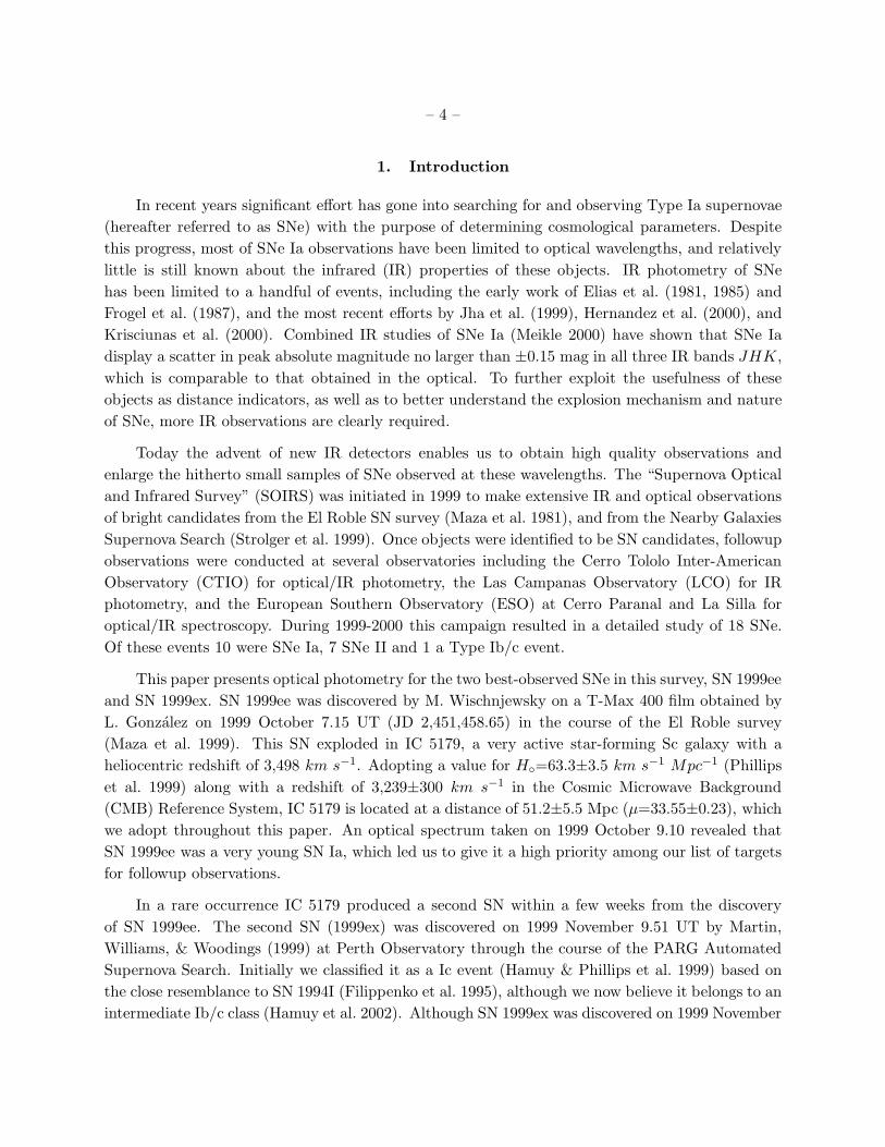
Figure 1 shows the filter bandpasses for both instruments compared to the standard ones defined

by Bessell (1990) and Hamuy et al. (2001). We obtained a few additional photometric observations

with the CTIO 1.5-m telescope as well as with the ESO NTT and Danish 1.54-m telescopes. Refer

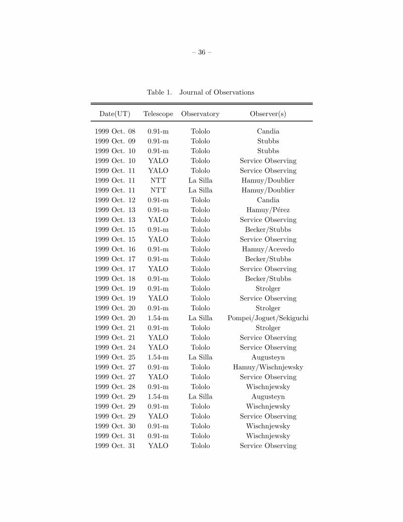
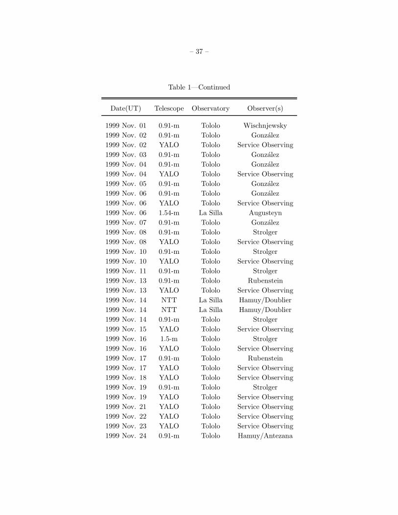
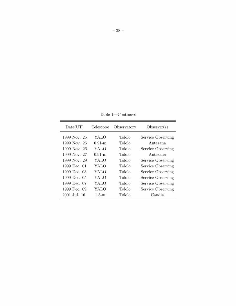
to Table 1 for the log of the observations, which includes the date of observation, telescope used,

observatory, and observer name(s).

In order to reduce the effects due to atmospheric extinction we determined the brightness of

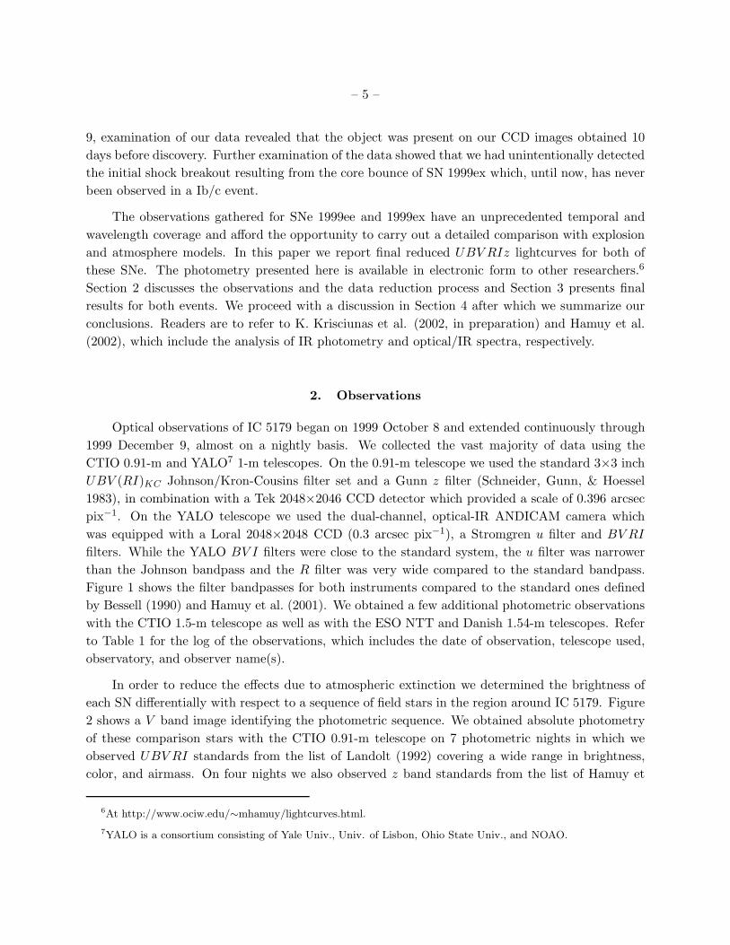
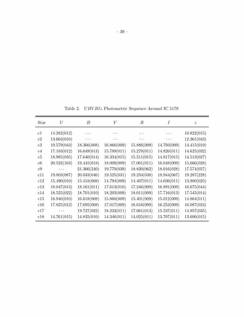
each SN differentially with respect to a sequence of field stars in the region around IC 5179. Figure

2 shows a V band image identifying the photometric sequence. We obtained absolute photometry

of these comparison stars with the CTIO 0.91-m telescope on 7 photometric nights in which we

observed UBV RI standards from the list of Landolt (1992) covering a wide range in brightness,

color, and airmass. On four nights we also observed z band standards from the list of Hamuy et

6At http://www.ociw.edu/∼mhamuy/lightcurves.html.

7YALO is a consortium consisting of Yale Univ., Univ. of Lisbon, Ohio State Univ., and NOAO.

– 6 –

al. (2001). In order to transform instrumental magnitudes to the standard Johnson/Kron-Cousins

system we assumed linear transformations of the following form,

U = u − kUX + CTU(u − b) + ZPU , (1)

B = b − kBX + CTB(b − v) + ZPB , (2)

V = v − kV X + CTV (b − v) + ZPV , (3)

R = r − kRX + CTR(v − r) + ZPR, (4)

I = i − kIX + CTI(v − i) + ZPI , (5)

Z = z − kzX + CTz(v − z) + ZPz, (6)

where U,B, V,R, I, Z refer to magnitudes in the standard system, u, b, v, r, i, z refer to instrumental

magnitudes measured with an aperture of 14 arcsec in diameter (the same employed by Landolt),

ki to the atmospheric extinction coefficient, X to airmass, CTi to the color term, and ZPi to the

zero-point of the transformation. For each photometric night we used least-squares fits to solve

for the photometric coefficients given above. Except for the U band the typical scatter in the

transformation equations amounted to 0.01-0.02 mag (standard deviation), thus confirming the

photometric quality of the night. For U the spread was typically 0.03-0.04 mag. Table 2 contains

the UBV RIz photometry of the sequence stars identified in Figure 2 along with the corresponding

errors in the mean.

From the many different photometric nights of the SOIRS program we noticed that the color

terms of the CTIO 0.91-m telescope varied little with time, thus allowing us to adopt average values.

This offered the advantage of reducing the number of fitting parameters in equations 1-6 during

the SN reductions. For the CTIO 1.5-m, NTT, and Danish 1.54-m telescopes we were also able

to derive average color terms from observations of Landolt standards on multiple nights. For the

YALO, on the other hand, we did not have observations of Landolt stars so we used the photometric

sequence itself to solve for color terms. From the many nights of data we could not see significant

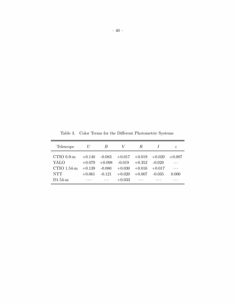
changes in these coefficients, thus allowing us to adopt average values. Table 3 summarizes the

average values for each telescope and associated filters. This table reveals that the color terms for

the instrumental U and B bands are generally large owing to the rapid sensitivity drop of CCDs

toward blue wavelengths, which effectively shifts the bandpasses to the red. Except for the YALO

R filter the remaining color terms are close to zero, thus implying a good match of the instrumental

bands to the standard system. The large color term for the YALO R filter is clearly not unexpected

owing to its non-standard width (see Figure 1).

Before performing photometry of the SNe, we subtracted late time templates of the parent

galaxy from all images in order to reduce light contamination using the method described by

Filippenko et al. (1986) and Hamuy et al. (1994a). We obtained good-seeing moonless UBV RIz

images of IC 5179 with the CTIO 1.5-m telescope on 2001 July 16, nearly two years after discovery

– 7 –

of the SNe. We took three images of IC 5179 in BV Iz and two RU images with an exposure

time of 300 seconds. We combined these to create deeper master images of the host galaxy for

the subtraction process. The procedure used for galaxy subtraction consisted of four steps, each of

which was performed with IRAF8 scripts. The steps included: (1) aligning the two images using

field star positions (coordinate registration); (2) matching the point spread function (PSF) of the

two images (PSF registration); (3) matching the flux scale of the two images (flux registration);

(4) subtracting the galaxy image from the SN+galaxy image. To avoid subtracting the local

photometric sequence from the subtracted image we restricted the subtraction to a small image

section around the host galaxy. With this approach the local standards remained unaffected by

the above procedure and we could proceed to carry out differential photometry for the SN and the

local standards from the same image.

Upon completing galaxy subtraction we performed differential photometry for all images of

the SNe using either aperture photometry (with the IRAF task PHOT) or PSF photometry (with

the IRAF task DAOPHOT), depending on the SN brightness. When photon noise exceeded 0.015

mag (the uncertainty in an individual photometric measurement caused by non-Poissonian errors)

for either SN, we used the more laborious PSF technique. The weather in Chile was very good

around 1999 October/November and the seeing values at CTIO and ESO were always below 2.5

arcsec, and generally between 1-1.5 arcsec (FWHM). Hence, we chose an aperture of 2 arcsec to

calculate instrumental magnitudes for the SNe and the comparison stars. Likewise, during PSF

photometry we used a PSF fitting radius of 2 arcsec. While this aperture kept the sky noise

reasonably low, it included a large fraction (∼90%) of the total stellar flux, thus minimizing errors

due to possible variations of the PSF across the image. For each frame we used the local standards

to solve for the photometric transformation coefficients (equations 1-6). The advantage of doing

differential photometry is that all stars in a frame are observed with the same airmass so that the

magnitude extinction is nearly the same for all stars, thus reducing the number of free parameters

in the transformation equations9. Moreover, having fixed the color terms to the average values, the

photometric transformation for a single night only involved solving the zero point for each filter.

Typically the scatter in the photometric transformation proved <0.02 mag (standard deviation).

8The Image Reduction and Analysis Facility (IRAF) is maintained and distributed by the Association of Univer-

sities for Research in Astronomy, under a cooperative agreement with the National Science Foundation.

9Note that we neglected here any color dependence of the extinction coefficient. In the B band where the second-

order extinction is the highest – 0.02 mag per airmass per unit color – we could have made an error of 0.01 mag

because of this assumption.

– 8 –

3. Results

3.1. SN 1999ee

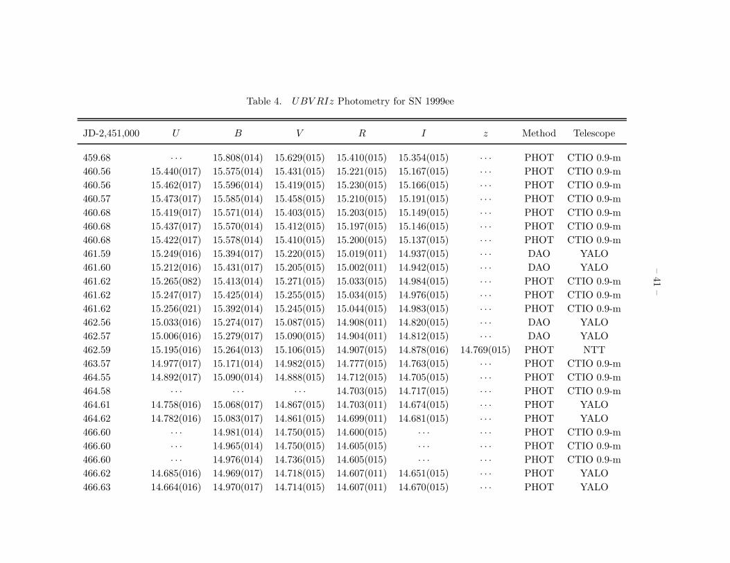
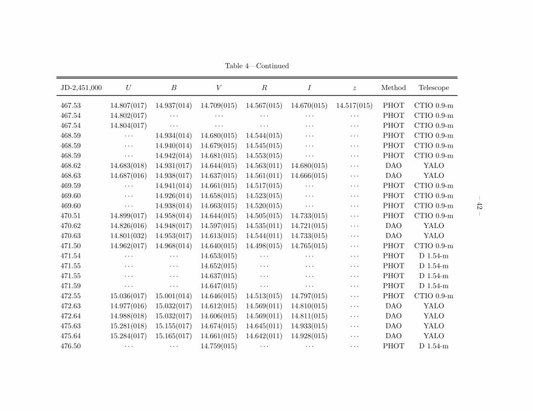
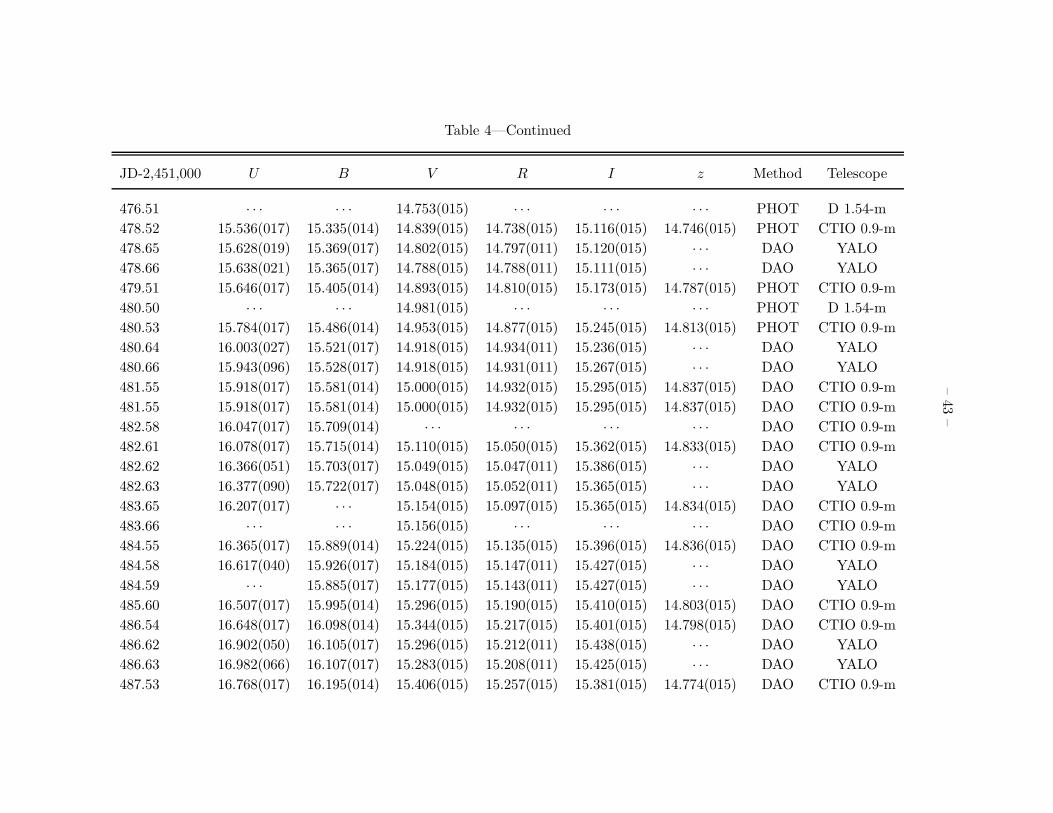
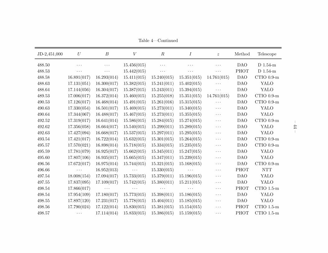
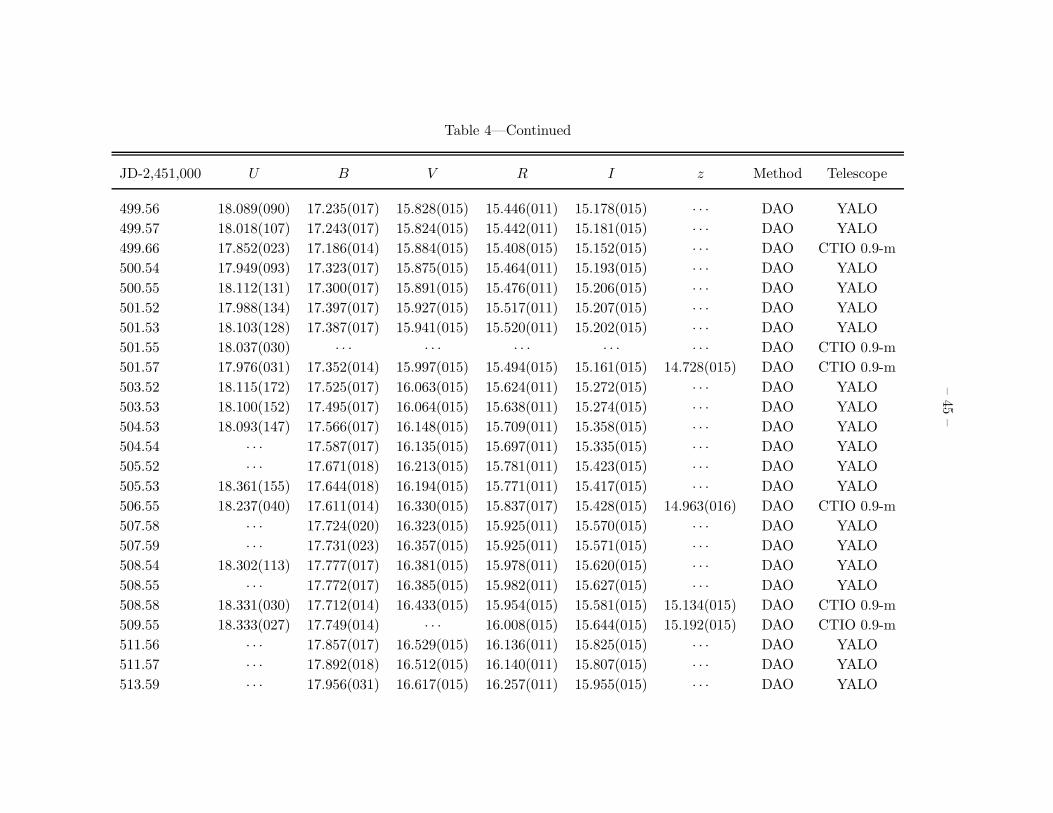
Table 4 lists the resulting UBV RIz photometry of SN 1999ee. The quoted errors correspond to

uncertainties owing to photon statistics. We adopted a minimum error of 0.015 mag in an individual

magnitude to account for uncertainties other than the Poissonian errors. This value is the typical

scatter that we observe from multiple CCD observations of bright stars whose Poissonian errors are

negligibly small. This table specifies whether we obtained the magnitudes via PSF fitting (DAO)

or aperture photometry (PHOT). We made observations for a total of 50 nights.

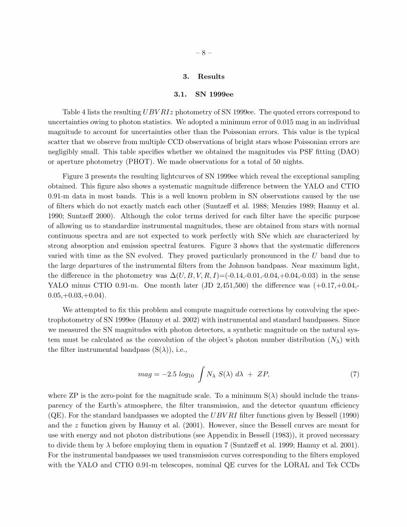
Figure 3 presents the resulting lightcurves of SN 1999ee which reveal the exceptional sampling

obtained. This figure also shows a systematic magnitude difference between the YALO and CTIO

0.91-m data in most bands. This is a well known problem in SN observations caused by the use

of filters which do not exactly match each other (Suntzeff et al. 1988; Menzies 1989; Hamuy et al.

1990; Suntzeff 2000). Although the color terms derived for each filter have the specific purpose

of allowing us to standardize instrumental magnitudes, these are obtained from stars with normal

continuous spectra and are not expected to work perfectly with SNe which are characterized by

strong absorption and emission spectral features. Figure 3 shows that the systematic differences

varied with time as the SN evolved. They proved particularly pronounced in the U band due to

the large departures of the instrumental filters from the Johnson bandpass. Near maximum light,

the difference in the photometry was ∆(U,B, V,R, I)=(-0.14,-0.01,-0.04,+0.04,-0.03) in the sense

YALO minus CTIO 0.91-m. One month later (JD 2,451,500) the difference was (+0.17,+0.04,-

0.05,+0.03,+0.04).

We attempted to fix this problem and compute magnitude corrections by convolving the spec-

trophotometry of SN 1999ee (Hamuy et al. 2002) with instrumental and standard bandpasses. Since

we measured the SN magnitudes with photon detectors, a synthetic magnitude on the natural sys-

tem must be calculated as the convolution of the object’s photon number distribution (Nλ) with

the filter instrumental bandpass (S(λ)), i.e.,

mag = −2.5 log10

∫Nλ S(λ) dλ + ZP, (7)

where ZP is the zero-point for the magnitude scale. To a minimum S(λ) should include the trans-

parency of the Earth’s atmosphere, the filter transmission, and the detector quantum efficiency

(QE). For the standard bandpasses we adopted the UBV RI filter functions given by Bessell (1990)

and the z function given by Hamuy et al. (2001). However, since the Bessell curves are meant for

use with energy and not photon distributions (see Appendix in Bessell (1983)), it proved necessary

to divide them by λ before employing them in equation 7 (Suntzeff et al. 1999; Hamuy et al. 2001).

For the instrumental bandpasses we used transmission curves corresponding to the filters employed

with the YALO and CTIO 0.91-m telescopes, nominal QE curves for the LORAL and Tek CCDs

– 9 –

used with both cameras, and an atmospheric transmission spectrum corresponding to one airmass.

Note that we did not include here mirror aluminum reflectivities, the dichroic transmission for the

YALO camera, and dewar window transmissions because we lacked such information.

To check if the resulting bandpasses provided a good model for those actually used at the tele-

scopes we computed synthetic magnitudes for spectrophotometric standards (Hamuy et al. 1994b)

and asked if the color terms derived from the synthetic magnitudes matched the observed values

given in Table 3. We could only do this calculation for the BV RIz filters since the spectropho-

tometric standards do not cover the entire U filter. We calculated synthetic color terms with

equations 2-6, where b, v, r, i, z are the synthetic magnitudes for the YALO and CTIO 0.91-m in-

strumental bandpasses and B,V,R, I, Z are the synthetic magnitudes derived from the standard

functions. Although we find an overall good agreement between the observed and synthetic color

terms, small differences are present which suggest some differences between the nominal and the

instrumental bandpasses used at the telescopes. Possible explanations for the differences are mirror

reflectivities or any transmissivity of other optical elements of the instruments employed (e.g. the

dichroic mirror used with YALO/ANDICAM). To solve this problem our approach consisted in

applying wavelength shifts to our nominal instrumental bandpasses until we were able to reproduce

exactly the measured color terms. The required shifts are summarized in Table 5. They are always

less than 100 A, except in the V and R YALO filters where they amount to 120 A and 180 A,

respectively. Figure 1 displays the resulting functions.

Armed with the best possible models for our instrumental bands we used the spectrophotome-

try of SN 1999ee to compute magnitude corrections (S-corrections, hereafter) that should allow us

to bring our observed photometry to the standard system. For the V filter the S-correction is

∆V = V − v − CTV (b − v) − ZPV , (8)

where V is the SN synthetic magnitude computed with the Bessell function, and b,v are the SN

synthetic magnitudes computed with the instrumental bandpasses. CTV is the color term for the

corresponding filter and ZPV is a zero point that can be obtained from the spectrophotometric

standards to better than 0.01 mag. Similar equations can be written for the other filters.

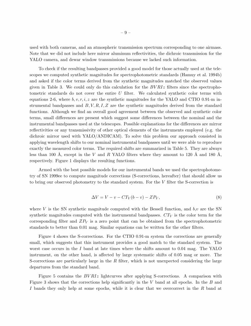
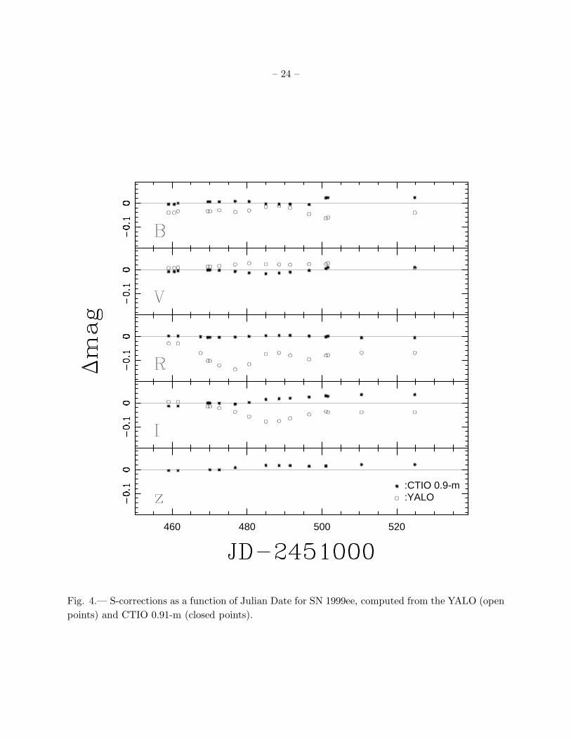
Figure 4 shows the S-corrections. For the CTIO 0.91-m system the corrections are generally

small, which suggests that this instrument provides a good match to the standard system. The

worst case occurs in the I band at late times where the shifts amount to 0.04 mag. The YALO

instrument, on the other hand, is affected by large systematic shifts of 0.05 mag or more. The

S-corrections are particularly large in the R filter, which is not unexpected considering the large

departures from the standard band.

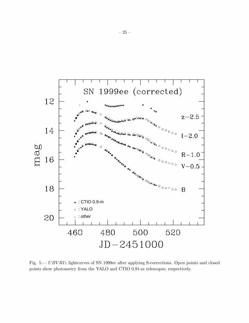
Figure 5 contains the BV RIz lightcurves after applying S-corrections. A comparison with

Figure 3 shows that the corrections help significantly in the V band at all epochs. In the B and

I bands they only help at some epochs, while it is clear that we overcorrect in the R band at

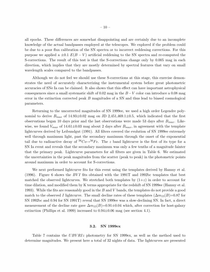
– 10 –

all epochs. These differences are somewhat disappointing and are certainly due to an incomplete

knowledge of the actual bandpasses employed at the telescopes. We explored if the problem could

be due to a poor flux calibration of the SN spectra or to incorrect reddening corrections. For this

purpose we applied a ±0.1 E(B − V ) artificial reddening to the SN spectra and re-computed the

S-corrections. The result of this test is that the S-corrections change only by 0.005 mag in each

direction, which implies that they are mostly determined by spectral features that vary on small

wavelength scales compared to the bandpasses.

Although we do not feel we should use these S-corrections at this stage, this exercise demon-

strates the need of accurately characterizing the instrumental system before great photometric

accuracies of SNe Ia can be claimed. It also shows that this effect can have important astrophysical

consequences since a small systematic shift of 0.02 mag in the B−V color can introduce a 0.08 mag

error in the extinction corrected peak B magnitudes of a SN and thus lead to biased cosmological

parameters.

Returning to the uncorrected magnitudes of SN 1999ee, we used a high order Legendre poly-

nomial to derive Bmax of 14.93±0.02 mag on JD 2,451,469.1±0.5, which indicated that the first

observations began 10 days prior and the last observations were made 53 days after Bmax. Like-

wise, we found Vmax of 14.61±0.03 mag about 2 days after Bmax, in agreement with the template

lightcurves derived by Leibundgut (1991). All filters covered the evolution of SN 1999ee extremely

well through maximum light, past the secondary maximum through the onset of the exponential

tail due to radioactive decay of 56Co→56Fe. The z band lightcurve is the first of its type for a

SN Ia event and reveals that the secondary maximum was only a few tenths of a magnitude fainter

that the primary peak. Lightcurve parameters for all filters are given in Table 6. We estimated

the uncertainties in the peak magnitudes from the scatter (peak to peak) in the photometric points

around maximum in order to account for S-corrections.

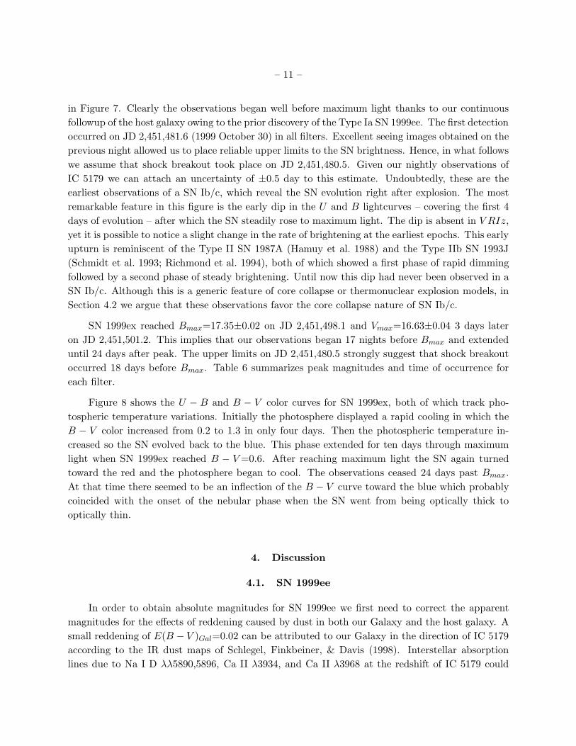
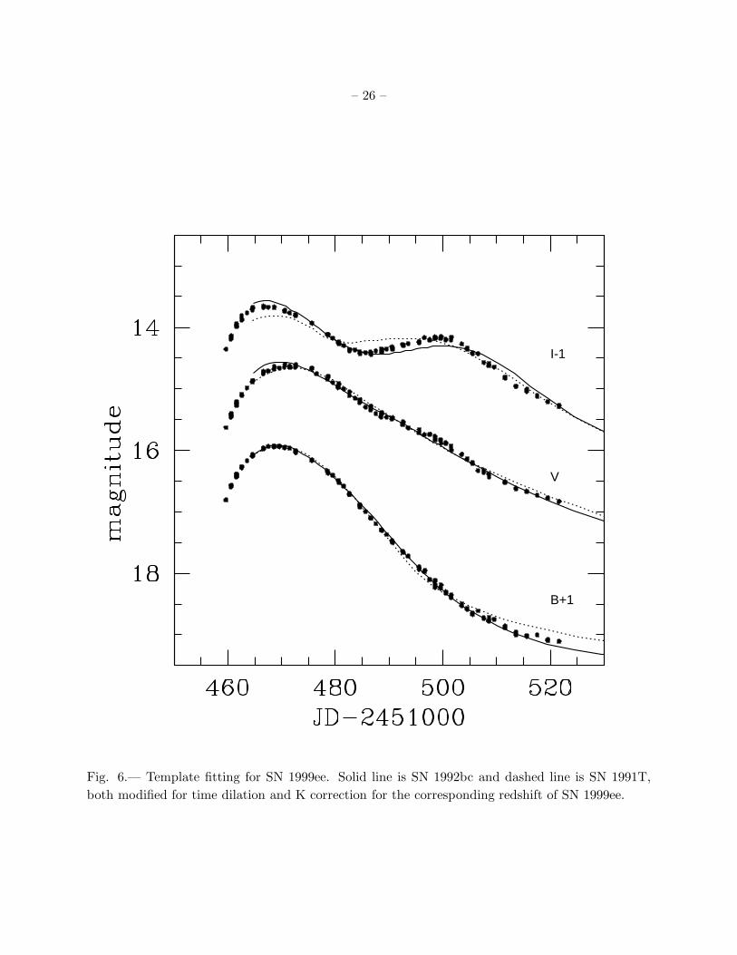
We next performed lightcurve fits for this event using the templates derived by Hamuy et al.

(1996). Figure 6 shows the BV I fits obtained with the 1991T and 1992bc templates that best

matched the observed lightcurves. We stretched both templates by (1+z) in order to account for

time dilation, and modified them by K terms appropriate for the redshift of SN 1999ee (Hamuy et al.

1993). While the fits are reasonably good in the B and V bands, the templates do not provide a good

match to the observed I lightcurve. The small decline rates of these templates (∆m15(B)=0.87 for

SN 1992bc and 0.94 for SN 1991T) reveal that SN 1999ee was a slow-declining SN. In fact, a direct

measurement of the decline rate gave ∆m15(B)=0.91±0.04 which, after correction for host-galaxy

extinction (Phillips et al. 1999) increased to 0.94±0.06 mag (see section 4.1).

3.2. SN 1999ex

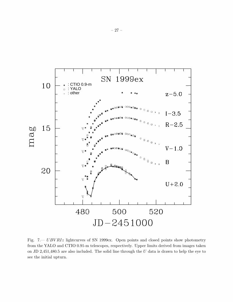
Table 7 contains the UBV RIz photometry for SN 1999ex, as well as the method used to

determine magnitudes. We present here a total of 32 nights of data. The lightcurves are presented

– 11 –

in Figure 7. Clearly the observations began well before maximum light thanks to our continuous

followup of the host galaxy owing to the prior discovery of the Type Ia SN 1999ee. The first detection

occurred on JD 2,451,481.6 (1999 October 30) in all filters. Excellent seeing images obtained on the

previous night allowed us to place reliable upper limits to the SN brightness. Hence, in what follows

we assume that shock breakout took place on JD 2,451,480.5. Given our nightly observations of

IC 5179 we can attach an uncertainty of ±0.5 day to this estimate. Undoubtedly, these are the

earliest observations of a SN Ib/c, which reveal the SN evolution right after explosion. The most

remarkable feature in this figure is the early dip in the U and B lightcurves – covering the first 4

days of evolution – after which the SN steadily rose to maximum light. The dip is absent in V RIz,

yet it is possible to notice a slight change in the rate of brightening at the earliest epochs. This early

upturn is reminiscent of the Type II SN 1987A (Hamuy et al. 1988) and the Type IIb SN 1993J

(Schmidt et al. 1993; Richmond et al. 1994), both of which showed a first phase of rapid dimming

followed by a second phase of steady brightening. Until now this dip had never been observed in a

SN Ib/c. Although this is a generic feature of core collapse or thermonuclear explosion models, in

Section 4.2 we argue that these observations favor the core collapse nature of SN Ib/c.

SN 1999ex reached Bmax=17.35±0.02 on JD 2,451,498.1 and Vmax=16.63±0.04 3 days later

on JD 2,451,501.2. This implies that our observations began 17 nights before Bmax and extended

until 24 days after peak. The upper limits on JD 2,451,480.5 strongly suggest that shock breakout

occurred 18 days before Bmax. Table 6 summarizes peak magnitudes and time of occurrence for

each filter.

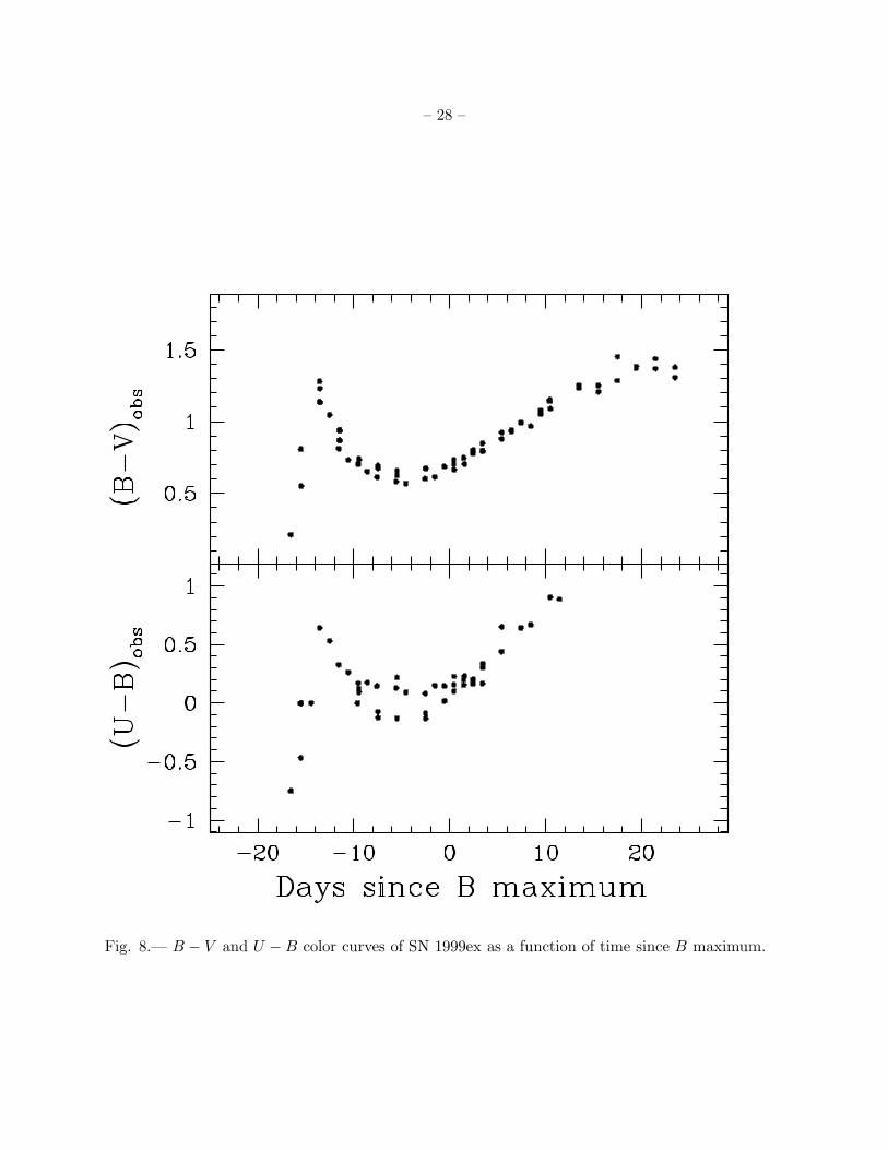
Figure 8 shows the U − B and B − V color curves for SN 1999ex, both of which track pho-

tospheric temperature variations. Initially the photosphere displayed a rapid cooling in which the

B − V color increased from 0.2 to 1.3 in only four days. Then the photospheric temperature in-

creased so the SN evolved back to the blue. This phase extended for ten days through maximum

light when SN 1999ex reached B − V =0.6. After reaching maximum light the SN again turned

toward the red and the photosphere began to cool. The observations ceased 24 days past Bmax.

At that time there seemed to be an inflection of the B − V curve toward the blue which probably

coincided with the onset of the nebular phase when the SN went from being optically thick to

optically thin.

4. Discussion

4.1. SN 1999ee

In order to obtain absolute magnitudes for SN 1999ee we first need to correct the apparent

magnitudes for the effects of reddening caused by dust in both our Galaxy and the host galaxy. A

small reddening of E(B − V )Gal=0.02 can be attributed to our Galaxy in the direction of IC 5179

according to the IR dust maps of Schlegel, Finkbeiner, & Davis (1998). Interstellar absorption

lines due to Na I D λλ5890,5896, Ca II λ3934, and Ca II λ3968 at the redshift of IC 5179 could

– 12 –

be clearly seen in the spectra of SN 1999ee, with equivalent widths (EW) of 2.3, 0.8, and 0.6 A,

respectively (Hamuy et al. 2002). This suggests that a non-negligible amount of absorption in

IC 5179 affected SN 1999ee. Calibrations between EW and reddening have been derived from high

resolution spectra of Galactic stars (Richmond et al. 1994; Munari & Zwitter 1997), but these are

only valid in the non-saturated regime (EW(Na I D)<0.8 A). Using SN data Barbon et al. (1990)

derived the relation E(B−V ) ∼ 0.25 EW (Na I D), which implies E(B−V )host=0.58 for SN 1999ee.

We believe, however, that this value is of little usefulness owing to the uncertain dust to gas ratio

around SNe (Hamuy et al. 2001).

Instead we can estimate the host galaxy’s reddening of SN 1999ee using the method described

by Phillips et al. (1999) and Lira (1995). The de-reddening technique consists in comparing the

observed colors of the SN to the intrinsic ones which are a function of the decline rate of the SN.

∆m15(B) itself can be affected by the extinction due to the change of the effective wavelength of

the B filter as the SN spectrum evolves (Phillips et al. 1999). From the direct measurement of

∆m15(B)obs=0.91±0.04 (after correction for time dilation and K-terms) and an internal reddening

of E(B − V )host=0.28±0.04 (see below), we derive a true decline rate of ∆m15(B)=0.94±0.06.

A direct comparison between the intrinsic colors (B−V )0 and (V −I)0 as predicted by Phillips

et al. (1999) and the observed colors at maximum light (after correction for Galactic reddening,

time dilation, and K-terms) yields E(B − V )max=0.39±0.11 and E(V − I)max=0.29±0.11. In

addition using colors from the exponential tail we determine E(B − V )tail=0.27±0.05. Taking the

weighted mean of E(B − V )max, E(B − V )tail, and 0.8E(V − I)max we obtain the final estimation

for host galaxy reddening E(B − V )host=0.28±0.04. Including Galactic extinction we get E(B −

V )total=0.30±0.04 which, following Phillips et al. (1999), leads to the following monochromatic

absorption values: AB=1.24±0.17, AV =0.94±0.13, and AI=0.55±0.07.

After applying these corrections to our BV I peak apparent magnitudes and using the dis-

tance modulus of 33.55±0.23 based on the galaxy redshift, we obtain final absolute peak mag-

nitudes of MB=-19.85±0.28, MV =-19.87±0.26, and MI=-19.43±0.24. For its decline rate of

∆m15(B)=0.94±0.06, SN 1999ee fits well with the peak luminosity-decline rate relation derived

by Phillips et al. (1999).

Instead of adopting a distance to solve for absolute magnitudes, we can now solve for the

distance to IC 5179 using the absolute magnitudes of SNe Ia recently calibrated with Cepheids.

Note that we are not using the previous redshift based absolute magnitudes so that this is an

independent test. The Cepheid-based absolute magnitudes (corrected for reddening and normalized

to a ∆m15(B)=1.10) of the SNe Ia calibrators used in Phillips et al. (1999) are MB=-19.61±0.09,

MV =-19.58±0.08, and MI=-19.29±0.10. For ∆m15(B)=0.94±0.06, the luminosity-decline rate

relation mentioned above predicts absolute magnitudes of MB=-19.72±0.12, MV =-19.67±0.11, and

MI=-19.34±0.12 for SN 1999ee. From the peak apparent magnitudes we obtain distance moduli of

µB=33.42±0.21, µV =33.35±0.17, and µI=33.46±0.14 hence yielding µavg=33.42±0.10 for IC 5179.

This value compares well with µ=33.55±0.23 derived from the galaxy redshift.

– 13 –

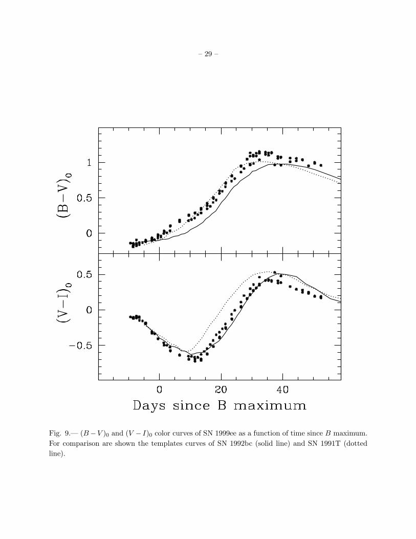
Figure 9 shows the (B − V )0 and (V − I)0 color curves of SN 1999ee corrected for E(B −

V )total=0.30, compared to the template curves of the slow-declining SNe 1992bc (solid line) and

SN 1991T (dotted line), both adjusted to match the colors of SN 1999ee at maximum light, time

dilated, and K-corrected. This comparison reveals that, although SN 1999ee had the typical trends

displayed by other SNe Ia, it is not possible to fit its color at all epochs with a single reddening

correction. SN 1992bc seems to provide a better match in V − I before day +30 but after that

epoch there is clear mismatch. SN 1991T, on the other hand, provides a good fit in B − V yet

a poor match in V − I. This demonstrates that SNe Ia with nearly the same decline rate do not

have identical color curves. These examples raise doubts about the derivation of reddening from

the shapes of the color curves, as advocated by Riess, Press, & Kirshner (1996). The method

implemented by Phillips et al. (1999), instead, does not use information on the shape of the color

curve but only the color at individual epochs.

4.2. SN 1999ex

SN 1999ex also showed clear absorption features due to interstellar lines of Na I D λλ5890,5896,

Ca II λ3934, and Ca II λ3968 at the redshift of IC 5179. The equivalent widths of 2.8, 1.8, and

0.9 A measured for these lines (Hamuy et al. 2002) suggest even more dust absorption than for

SN 1999ee. As mentioned above, however, it proves difficult to derive dust absorption from in-

terstellar lines owing to the very uncertain dust to gas ratio around SNe. A lower limit to the

peak absolute magnitudes of SN 1999ex can be derived assuming E(B − V )Gal=0.02 (Schlegel,

Finkbeiner, & Davis 1998). Omitting K-corrections (which are expected to be <0.02 mag, assum-

ing the K-terms for SNe Ib/c are similar for SNe Ia), we get MB<-16.28±0.23, MV <-16.98±0.23,

and MI<-17.61±0.23 for SN 1999ex. Assuming that the amount of reddening affecting SN 1999ex is

not radically different than E(B−V )host=0.28±0.04 derived from SN 1999ee we get absolute mag-

nitudes which may be considered representative of what the actual reddening might give. With this

assumption we obtain MB=-17.44±0.28, MV =-17.86±0.26, and MI=-18.12±0.24. These calcula-

tions illustrate how including host galaxy reddening affect the absolute magnitudes and, perhaps

more importantly, the bolometric lightcurve (see below).

Although the initial dip and UV excess observed in SN 1999ex had never been observed before

among Ib/c events, it was also observed in the Type II SN 1987A (Hamuy et al. 1988) and the Type

IIb SN 1993J (Schmidt et al. 1993; Richmond et al. 1994). For these SNe II it is thought that the

initial dip corresponded to a phase of adiabatic cooling that ensued the initial UV flash caused by

shock emergence which super-heated and accelerated the photosphere. The following brightening is

attributed to the energy deposited behind the photosphere by the radioactive decay of 56Ni→56Co

and 56Co→56Fe. Although the lightcurve of SN 1999ex bears qualitative resemblance to SN 1987A

and SN 1993J, in those cases the initial peaks were relatively brighter and the dips in the lightcurves

occurred ∼8 days after explosion compared to 4 days in SN 1999ex. This suggests that SN 1999ex

also was a core collapse SN and that the photometric differences could be due to the hydrogen that

– 14 –

the progenitors of SN 1987A and SN 1993J were able to retain. Woosley et al. (1987) computed

Type Ib SN models consisting of the explosion of a 6.2 M⊙ helium core. Their Figure 7 shows the

bolometric luminosities of three models with different explosion energies and 56Ni nucleosynthesis.

Despite the different lightcurve shapes and peak luminosities, all three models show an initial peak

followed by a dip a few days later and the subsequent brightening caused by 56Ni → 56Co →56Fe,

making them good models for SN 1999ex.

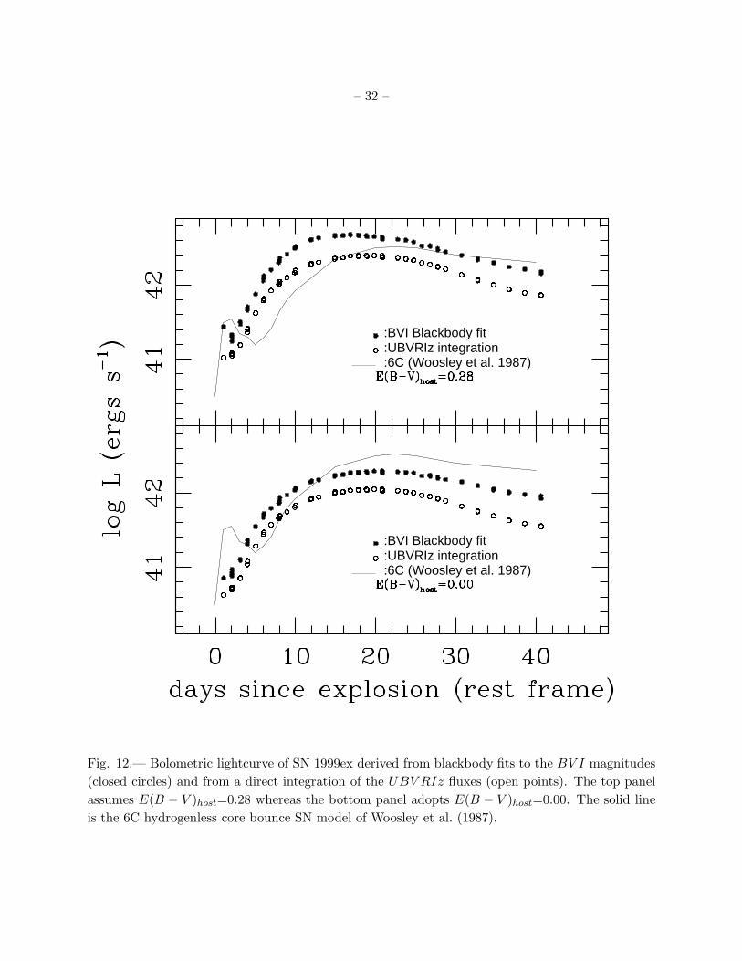
We proceed now to compute a bolometric lightcurve for SN 1999ex in order to carry out a

comparison with the models. A first approach consists in performing a blackbody (BB) fit at each

epoch and derive analytically the total flux from the corresponding Planck function. Our fitting

procedure consists in computing synthetic magnitudes in the Vega system (Hamuy et al. 2001)

for BB curves reddened by E(B − V )Gal=0.02 and E(B − V )host=0.28, performing a least-squares

fit to the SN BV I magnitudes, and deriving the color temperature and angular radius that yield

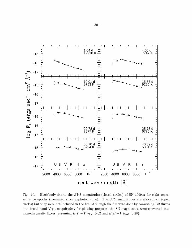
the best match to the observed photometry. Figure 10 illustrates the fits for eight representative

epochs. Note that, while the BB curve provides excellent fits during the first days of SN evolution,

by day 4 since explosion the observed U flux begins to fall below the BB curve. This is a result

of the strong line blanketing at these wavelengths, assuming the opacities for SNe Ib/c are similar

to SNe Ia (Pinto & Eastman 2000). Note also that, although the R and z magnitudes are not

included in the fits, they match well the BB curves derived from the BV I photometry. Table

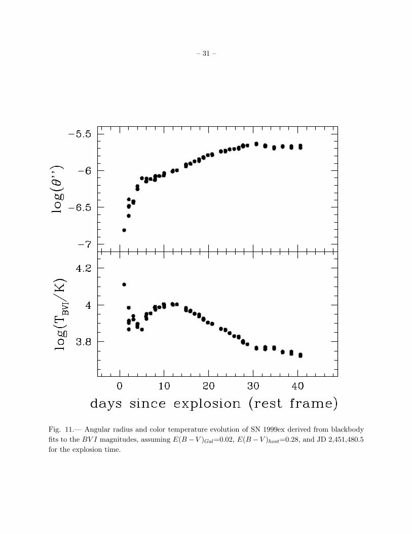
8 summarizes the parameters yielded by the BB fits for all epochs. Figure 11 shows that the

photospheric angular radius showed a steady increase which reflects the expansion of the SN ejecta.

During the first 4 days the photospheric temperature dropped due to the adiabatic cooling that

followed shock breakout, after which the temperature increased due to radioactive heating and then

dropped again owing to expansion. Note that, as expected, this curve bears close resemblance to

the color curves shown in Figure 8. The resulting bolometric lightcurve is plotted in the top panel

of Figure 12 (closed circles) and the corresponding values can be found in Table 8. For comparison

the bottom panel shows the curve obtained by assuming E(B − V )host=0.00.

An alternative route to derive bolometric fluxes is to perform a direct integration of the SN

UBV RIz broad-band magnitudes. For this purpose we use the UBV RIz magnitudes of Vega

(Hamuy et al. 1992, 2001) and its spectral energy distribution (Hayes 1985) to derive conversion

factors between broad-band magnitudes and monochromatic fluxes for the standard photometric

system shown in Figure 1. With these assumptions a zero magnitude star has monochromatic

fluxes of (3.98,6.43,3.67,2.23,1.17,0.82)×10−9 ergs sec−1 cm−2 A−1 for U,B, V,R, I, z, which have

equivalent wavelengths of 3570, 4413, 5512, 6585, 8068, and 9058 A, respectively. The resulting

U − z bolometric fluxes are listed in Table 8 and shown with open circles in Figure 12, both

for E(B − V )host=0.28 (top) and E(B − V )host=0.00 (bottom). Since the SN emitted more flux

beyond the U − z wavelength range, this approach is expected to give a lower limit to the actual

luminosity. Not surprisingly, the resulting fluxes lie well below the BB fluxes. The BB fits to the

BV I magnitudes may also underestimate the true flux by a few dex owing to line blanketing in

the B band. On the other hand, flux redistribution of the missing B flux could show up in the V I

– 15 –

bands and compensate for this flux deficit. Without a detailed atmosphere model for SNe Ib/c it

proves difficult to quantify the difference between the BB and the true SN luminosity. In the case

of SN 1987A – the SN with the best wavelength coverage – the BV I BB fit yields a flux ∼0.05

dex greater than the U→M bolometric flux of Suntzeff & Bouchet (1990), throughout the optically

thick phase of the SN. We believe therefore that the BB fits to SN 1999ex are probably within 0.1

dex from the true bolometric luminosity.

Figure 12 (top) reveals that the major difference between the BB and the U − z curves is

that the initial dip is not present in the U − z integration. This is due to the fact that the

SN photosphere was initially hot so that a significant fraction of the total flux was emitted at

wavelengths shorter than 3500 A. The BB fit on the other hand, provides such an excellent fit to

the U − z magnitudes at these epochs (Figure 10) that it must provide a better approximation to

the true flux. Figure 12 (bottom) also reveals that the initial dip is less obvious in the BB curve

when we assume E(B − V )host=0.00. Although this hypothesis is very unlikely given the strong

interstellar absorption lines in the spectrum of SN 1999ex, this is illustrative of the effect reddening

has on the bolometric lightcurve of SN 1999ex, which will in turn affect future calculations of the

progenitor system.

Among the three SN Ib models of Woosley et al. (1987) model 6C – characterized by a kinetic

energy of 2.73×1051 ergs and 0.16 M⊙ of 56Ni – provides the best match to the BB lightcurve

of SN 1999ex (Figure 12, top panel). The agreement is remarkable considering that we are not

attempting to adjust the parameters. The initial peak and subsequent dip have approximately the

right luminosities although the evolution of SN 1999ex was somewhat faster. The following rise

and post-maximum evolution is well described by the model.

The observation of the tail of the shock wave breakout in SN 1999ex and the initial dip in

the lightcurve provides us with an insight on the type of progenitor system for SNe Ib/c. Several

different models have been proposed as progenitors for this type of SNe. One possibility is an ac-

creting white dwarf which may explode via thermal detonation upon reaching the Chandrasekhar

mass (Sramek, Panagia, & Weiler 1984; Branch & Nomoto 1986). These models are expected to

produce lightcurves with an initial peak that corresponds to the emergence of the burning front, a

fast luminosity drop due to adiabatic expansion, and a subsequent rise caused by radioactive heat-

ing. Given the compact nature of the progenitor (∼1,800 km) the cooling time scale by adiabatic

expansion is only a few minutes (P. Hoflich 2002, private communication) and the lightcurve is

entirely governed by radioactive heating (Hoflich & Khokhlov 1996). Hence, these models are not

expected to show an early dip at a few days past explosion as is observed in SN 1999ex. The second

and more favored model for SNe Ib/c consists of core collapse of massive stars (MZAMS > 8 M⊙)

which lose their outer H envelope before explosion. Within the core collapse models, there are two

basic types of progenitor systems: 1) a massive (MZAMS > 35 M⊙) star which undergoes strong

stellar winds and becomes a Wolf-Rayet star at the time of explosion (Woosley, Langer & Weaver

1993), and 2) an exchanging binary system (Shigeyama et al. 1990; Nomoto et al. 1994; Iwamoto

et al. 1994) for less massive stars. The resulting SNe have bolometric lightcurves containing an

– 16 –

initial shock breakout followed by a dip. Since the initial radii of these progenitors are ∼100 times

greater than that of white dwarfs, the dip occurs several days after explosion (Woosley et al. 1987;

Shigeyama et al. 1990; Woosley, Langer & Weaver 1993, 1995), very much like SN 1999ex.

Although a detailed modeling of SN 1999ex is beyond the scope of this paper, the fact that we

were able to observe the initial shock break out followed by a dip within four days since explosion

lends support to the idea that SNe Ib/c are due to the core collapse of massive progenitors rather

than the thermonuclear disruption of white dwarfs. This is a prediction that could not have been

decisively made prior to these observations.

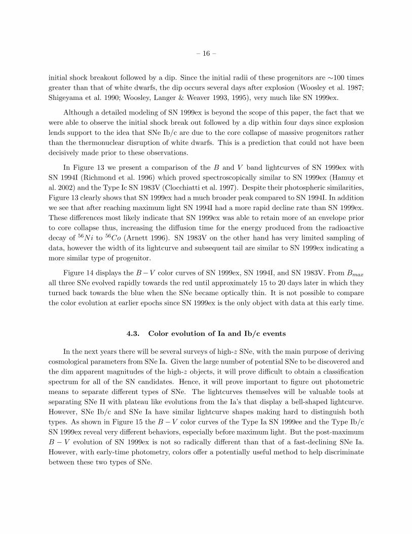
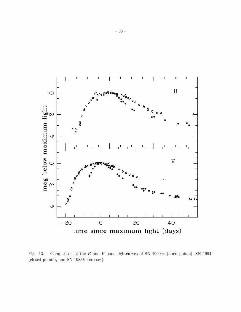
In Figure 13 we present a comparison of the B and V band lightcurves of SN 1999ex with

SN 1994I (Richmond et al. 1996) which proved spectroscopically similar to SN 1999ex (Hamuy et

al. 2002) and the Type Ic SN 1983V (Clocchiatti et al. 1997). Despite their photospheric similarities,

Figure 13 clearly shows that SN 1999ex had a much broader peak compared to SN 1994I. In addition

we see that after reaching maximum light SN 1994I had a more rapid decline rate than SN 1999ex.

These differences most likely indicate that SN 1999ex was able to retain more of an envelope prior

to core collapse thus, increasing the diffusion time for the energy produced from the radioactive

decay of 56Ni to 56Co (Arnett 1996). SN 1983V on the other hand has very limited sampling of

data, however the width of its lightcurve and subsequent tail are similar to SN 1999ex indicating a

more similar type of progenitor.

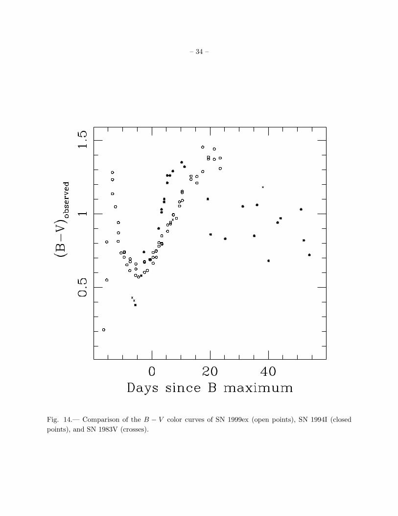
Figure 14 displays the B−V color curves of SN 1999ex, SN 1994I, and SN 1983V. From Bmax

all three SNe evolved rapidly towards the red until approximately 15 to 20 days later in which they

turned back towards the blue when the SNe became optically thin. It is not possible to compare

the color evolution at earlier epochs since SN 1999ex is the only object with data at this early time.

4.3. Color evolution of Ia and Ib/c events

In the next years there will be several surveys of high-z SNe, with the main purpose of deriving

cosmological parameters from SNe Ia. Given the large number of potential SNe to be discovered and

the dim apparent magnitudes of the high-z objects, it will prove difficult to obtain a classification

spectrum for all of the SN candidates. Hence, it will prove important to figure out photometric

means to separate different types of SNe. The lightcurves themselves will be valuable tools at

separating SNe II with plateau like evolutions from the Ia’s that display a bell-shaped lightcurve.

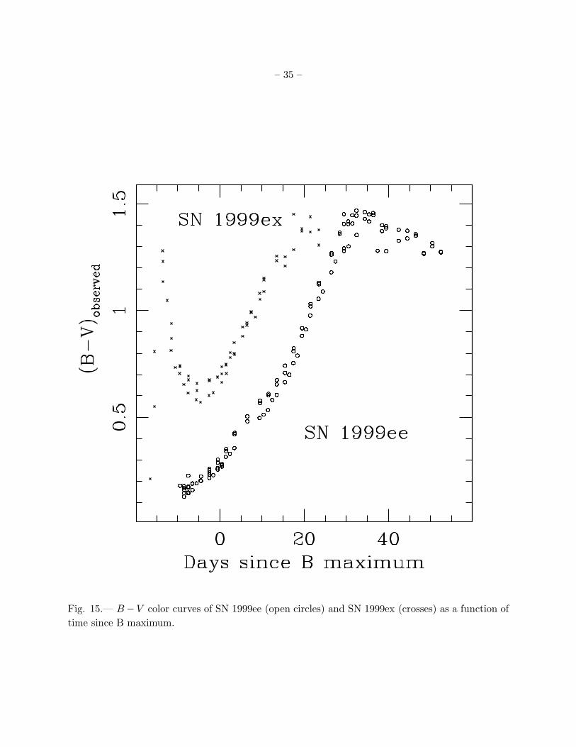
However, SNe Ib/c and SNe Ia have similar lightcurve shapes making hard to distinguish both

types. As shown in Figure 15 the B − V color curves of the Type Ia SN 1999ee and the Type Ib/c

SN 1999ex reveal very different behaviors, especially before maximum light. But the post-maximum

B − V evolution of SN 1999ex is not so radically different than that of a fast-declining SNe Ia.

However, with early-time photometry, colors offer a potentially useful method to help discriminate

between these two types of SNe.

– 17 –

5. Conclusions

In a rare occurrence two SNe were observed simultaneously in IC 5179 at a redshift of z = 0.01

between 1999 October-December. For each image of these SNe we performed galaxy subtraction of

late time images of their host galaxy after which we extracted UBV RIz magnitudes. We obtained

well-sampled lightcurves including the first z band observations for a SN Ia and SN Ib/c.

Observations of the Type Ia SN 1999ee span from 10 days prior to Bmax to 53 days afterwards.

SN 1999ee was characterized by a slow decline rate of ∆m15(B)=0.94±0.06. We estimate a value

of host-galaxy reddening of 0.28±0.04 which we use to derive reddening-free peak absolute magni-

tudes of MB=-19.85±0.28, MV =-19.87±0.26, and MI=-19.43±0.24. SN 1999ee is among the most

luminous SNe Ia and fits well in the peak luminosity-decline rate relation for SNe Ia.

Near maximum we find systematic differences ∼0.05 mag in photometry measured with two

different telescopes, even though the photometry is reduced to the same local standards around

the supernova using the specific color terms for each instrumental system. We use models for our

bandpasses and spectrophotometry of SN 1999ee to derive magnitude corrections (S-corrections)

and remedy this problem. This exercise demonstrates the need of accurately characterizing the

instrumental system before great photometric accuracies of Type Ia supernovae can be claimed. It

also shows that this effect can have important astrophysical consequences since a small systematic

shift of 0.02 mag in the B − V color can introduce a 0.08 mag error in the extinction corrected

peak B magnitudes of a supernova and thus lead to biased cosmological parameters.

The data for the second SN observed in this galaxy – Type Ib/c SN 1999ex – present us with

the first ever observed shock breakout of a supernova of this class. These observations show that

shock breakout occurred 18 days before Bmax and support the idea that Type Ib/c supernovae are

due to core collapse of massive stars rather than thermonuclear disruption of white dwarfs. The

comparison of the lightcurves of SN 1999ex to other SNe Ic events like SN 1983V and SN 1994I

reveals large photometric differences among this class of objects, probably due to variations in

the properties of the envelopes of their progenitors and/or explosion energies. Future theoretical

modeling of this event along with spectral analysis and construction of a bolometric lightcurve will

provide insight on relevant parameters describing its progenitor.

M.S. is very grateful to Cerro Tololo for allocating an office and providing computer facilities

while in La Serena (where the first draft of this paper was prepared) as well as to Mark Wagner for

providing computer facilities in Tucson. We are very grateful to the YALO team for their service

observing observations for this program and to the CTIO and ESO visitor support staffs for their

assistance in the course of our observing runs. M.S. acknowledges support by the Hubble Space

Telescope grant HST GO-07505.02-96A. M.H. acknowledges support provided by NASA through

Hubble Fellowship grant HST-HF-01139.01-A awarded by the Space Telescope Science Institute,

which is operated by the Association of Universities for Research in Astronomy, Inc., for NASA, un-

der contract NAS 5-26555. This research has made use of the NASA/IPAC Extragalactic Database

– 18 –

(NED), which is operated by the Jet Propulsion Laboratory, California Institute of Technology,

under contract with the National Aeronautics and Space Administration. This research has made

use of the SIMBAD database, operated at CDS, Strasbourg, France.

REFERENCES

Arnett, W. D. 1996, Supernovae and Nucleosynthesis (Princeton:Princeton Univ. Press)

Barbon, R., Benetti, S., Capellaro, E., Rosino, L., & Turatto, M. 1990, A&A, 237, 79

Bessell, M. S. 1983, PASP, 95, 480

Bessell, M. S. 1990, PASP, 102, 1181

Branch, D., & Nomoto, K. 1986, A&A, 164, L13

Clocchiatti, A., et al. 1997, ApJ, 483, 675

Elias, J. H., Frogel, J. A., Hackwell, J. A., & Persson, S. E. 1981, ApJ, 251, L13

Elias, J. H., Matthews, K., Neugebauer, G., & Persson, S. E. 1985, ApJ, 296, 379

Filippenko, A. V., Porter, A. C., Sargent, W. L. W., & Schneider, D. P. 1986, AJ, 92, 1341

Filippenko, A. V., et al. 1995, ApJ, 450, L11

Frogel, J. A., Gregory, B., Kawara, K., Laney, D., Phillips, M. M., Terndrup, D., Vrba, F., &

Whitford, A. E. 1987, ApJ, 315, L129

Hamuy, M., Suntzeff, N. B., Gonzalez, R., & Martin, G. 1988, AJ, 95, 63

Hamuy, M., Suntzeff, N. B., Bravo, J., & Phillips, M. M. 1990, PASP, 102, 888

Hamuy, M., Walker, A. R., Suntzeff, N. B., Gigoux, P., Heathcote, S. R., & Phillips, M. M. 1992,

PASP, 104, 533

Hamuy, M., Phillips, M. M., Wells, L. A., & Maza, J. 1993, PASP, 105, 787

Hamuy, M., et al. 1994a, AJ, 108, 2226

Hamuy, M., Suntzeff, N. B., Heathcote, S. R., Walker, A. R., Gigoux, P., & Phillips, M. M. 1994b,

PASP, 106, 566

Hamuy, M., Phillips, M. M., Suntzeff, N. B., Schommer, R. A., Maza, J., Smith, R. C., Lira, P., &

Aviles, R. 1996, AJ, 112, 2438

Hamuy, M., & Phillips, M. M. 1999, IAU Circ. 7310

– 19 –

Hamuy, M., et al. 2001, ApJ, 558, 615

Hamuy, M., et al. 2002, AJ, 124, 417

Hayes, D. S. 1985, in Calibration of Fundamental Stellar Quantities, ed. D. S. Hayes, L. E. Pasinetti,

& A. G. Philip (Dordrecht: Reidel), 225

Hernandez, M., et al. 2000, MNRAS, 319, 223

Hoflich, P., & Khokhlov, A. 1996, ApJ, 457, 500

Iwamoto, K., Nomoto, K., Hoflich, P., Yamaoka, H., Kumagai, S., & Shigeyama, T. 1994, ApJ,

437, L115

Jha, S., et al. 1999, ApJS, 125, 73

Krisciunas, K., Hastings, N. C., Loomis, K., McMillan, R., Rest, A., Riess, A. G., & Stubbs, C.

2000, ApJ, 539, 658

Landolt, A. U. 1992, AJ, 104, 340

Leibundgut, B., Tammann, G. A., Cadonau, R., & Cerrito, D. 1991, A&AS, 89, 537

Lira, P. 1995, M.S. thesis, University of Chile

Martin, R., Williams, A., & Woodings, S. 1999, IAU Circ. 7310

Maza, J., Wischnejewsky, M., Torres, C., Gonzalez, L., Costa, E., & Wroblewski, H. 1981, PASP,

93, 239

Maza, J., Hamuy, M., Wischnjewsky, M., Gonzalez, L., Candia, P., & Lidman, C. 1999, IAU Circ.

7272

Meikle, W. P. S. 2000, MNRAS, 314, 782

Menzies, J. W. 1989, MNRAS, 237, 21

Munari, U., & Zwitter, T. 1997, A&A, 318, 269

Nomoto, K., Yamaoka, H., Pols, O. R., van den Heuvel, E. P. J., Iwamoto, K., Kumakai, S., &

Shigeyama, T. 1994, Nature, 371, 227

Phillips, M. M., Lira, P., Suntzeff, N. B., Schommer, R. A., Hamuy, M., & Maza, J. 1999, AJ, 118,

1766

Pinto, P. A., & Eastman, R. G. 2000, ApJ, 530, 757

Richmond, M. W., Treffers, R. R., Filippenko, A. V., Paik, Y., Leibundgut, B., Schulman, E., &

Cox, C. V. 1994, AJ, 107, 1022

– 20 –

Richmond, M. W., et al. 1996, AJ, 111, 327

Riess, A. G., Press, W. H., & Kirshner, R. P. 1996, ApJ, 473, 88

Schlegel, D. J., Finkbeiner, D. P., & Davis, M. 1998, ApJ, 500, 525

Schmidt, B. P., et al. 1993, Nature, 364, 600

Schneider, D. P., Gunn, J. E., & Hoessel, J. G., 1983, ApJ, 264, 337

Shigeyama, T., Nomoto, K., Tsujimoto, T., & Hashimoto, M. 1990, ApJ, 361, L23

Sramek, R. A., Panagia, N., & Weiler, K. W. 1984, ApJ, 285, L59

Suntzeff, N. B., Hamuy, M., Martin, G., Gomez, A., & Gonzalez, R. 1988, AJ, 96, 1864

Suntzeff, N. B., & Bouchet, P. 1990, AJ, 99, 650

Suntzeff, N. B., et al. 1999, AJ, 117, 1175

Suntzeff, N. B. 2000, in Cosmic Explosions, Tenth Astrophysics Conference, ed. S.S. Holt, & W.W.

Zhang (AIP, New York), 65

Strolger, L. G., et al. 1999, BAAS, 195, 3801

Woosley, S. E., Pinto, P. A., Martin, P. G., & Weaver, T. A. 1987, ApJ, 318, 664

Woosley, S. E., Langer, N., Weaver, T. A. 1993, ApJ, 411, 823

Woosley, S. E., Langer, N., Weaver, T. A. 1995, ApJ, 448, 315

This preprint was prepared with the AAS LATEX macros v5.0.

– 21 –

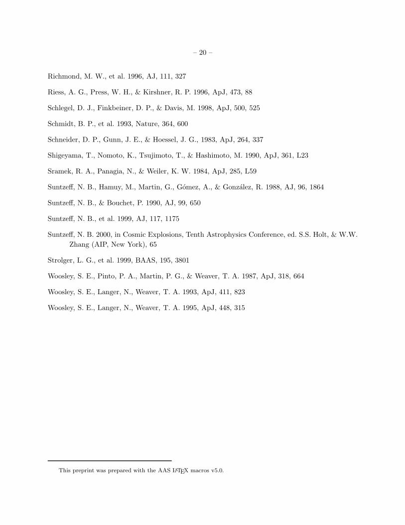
Fig. 1.— Comparison of UBV RIz bandpasses for the YALO (dashed line) and CTIO 0.91-m

(dotted line) telescopes. Each of these curves corresponds to the multiplication of the filter trans-

mission curve, CCD quantum efficiency, and the atmospheric continuum transmission spectrum

for one airmass. Atmospheric line opacity is not included in these bandpasses because they are

used with spectra containing telluric lines. Also shown (solid line) are the Bessell (1990) standard

Johnson/Kron-Cousins functions and the standard z function defined by Hamuy et al. (2001).

– 22 –

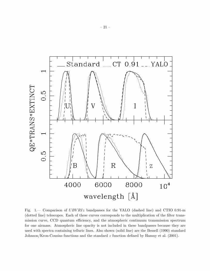
Fig. 2.— V band CCD image of SN 1999ee and SN 1999ex in IC 5179 taken on 1999 Nov. 17.

The photometric sequence stars are labeled. The right panel displays the galaxy subtracted image

clearly revealing both SNe. To avoid subtracting the local photometric sequence from the subtracted

image we restricted the subtraction to the image section around the host galaxy.

– 23 –

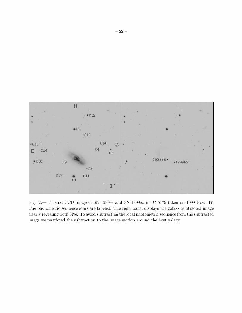
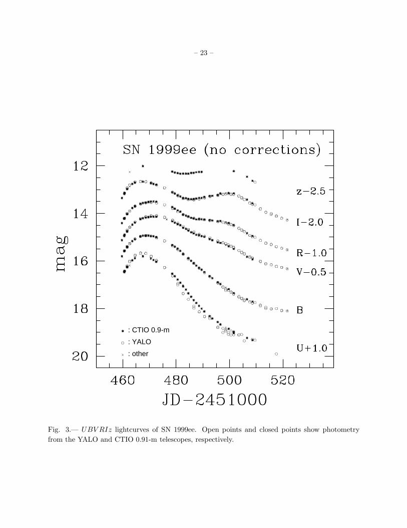
: CTIO 0.9-m

: YALO

: other

Fig. 3.— UBV RIz lightcurves of SN 1999ee. Open points and closed points show photometry

from the YALO and CTIO 0.91-m telescopes, respectively.

– 24 –

460 480 500 520

:YALO:CTIO 0.9-m

Fig. 4.— S-corrections as a function of Julian Date for SN 1999ee, computed from the YALO (open

points) and CTIO 0.91-m (closed points).

– 25 –

: CTIO 0.9-m

: YALO

: other

Fig. 5.— UBV RIz lightcurves of SN 1999ee after applying S-corrections. Open points and closed

points show photometry from the YALO and CTIO 0.91-m telescopes, respectively.

– 26 –

B+1

V

I-1

Fig. 6.— Template fitting for SN 1999ee. Solid line is SN 1992bc and dashed line is SN 1991T,

both modified for time dilation and K correction for the corresponding redshift of SN 1999ee.

– 27 –

: CTIO 0.9-m: YALO: other

Fig. 7.— UBV RIz lightcurves of SN 1999ex. Open points and closed points show photometry

from the YALO and CTIO 0.91-m telescopes, respectively. Upper limits derived from images taken

on JD 2,451,480.5 are also included. The solid line through the U data is drawn to help the eye to

see the initial upturn.

– 28 –

Fig. 8.— B − V and U − B color curves of SN 1999ex as a function of time since B maximum.

– 29 –

Fig. 9.— (B −V )0 and (V − I)0 color curves of SN 1999ee as a function of time since B maximum.

For comparison are shown the templates curves of SN 1992bc (solid line) and SN 1991T (dotted

line).

– 30 –

-17

-16

-151.04 d12918 K

4.00 d7747 K

-17

-16

-1510.01 d9753 K

15.87 d9225 K

-17

-16

-15

20.78 d7877 K

25.75 d6776 K

2000 4000 6000 8000

-17

-16

-1530.70 d5794 K

U B V R I z

2000 4000 6000 8000

40.62 d5381 K

U B V R I z

Fig. 10.— Blackbody fits to the BV I magnitudes (closed circles) of SN 1999ex for eight repre-

sentative epochs (measured since explosion time). The URz magnitudes are also shown (open

circles) but they were not included in the fits. Although the fits were done by converting BB fluxes

into broad-band Vega magnitudes, for plotting purposes the SN magnitudes were converted into

monochromatic fluxes (assuming E(B − V )Gal=0.02 and E(B − V )host=0.28).

– 31 –

Fig. 11.— Angular radius and color temperature evolution of SN 1999ex derived from blackbody

fits to the BV I magnitudes, assuming E(B −V )Gal=0.02, E(B −V )host=0.28, and JD 2,451,480.5

for the explosion time.

– 32 –

:BVI Blackbody fit:UBVRIz integration:6C (Woosley et al. 1987)

:BVI Blackbody fit:UBVRIz integration:6C (Woosley et al. 1987)

Fig. 12.— Bolometric lightcurve of SN 1999ex derived from blackbody fits to the BV I magnitudes

(closed circles) and from a direct integration of the UBV RIz fluxes (open points). The top panel

assumes E(B − V )host=0.28 whereas the bottom panel adopts E(B − V )host=0.00. The solid line

is the 6C hydrogenless core bounce SN model of Woosley et al. (1987).

– 33 –

Fig. 13.— Comparison of the B and V -band lightcurves of SN 1999ex (open points), SN 1994I

(closed points), and SN 1983V (crosses).

– 34 –

Fig. 14.— Comparison of the B − V color curves of SN 1999ex (open points), SN 1994I (closed

points), and SN 1983V (crosses).

– 35 –

Fig. 15.— B − V color curves of SN 1999ee (open circles) and SN 1999ex (crosses) as a function of

time since B maximum.

– 36 –

Table 1. Journal of Observations

Date(UT) Telescope Observatory Observer(s)

1999 Oct. 08 0.91-m Tololo Candia

1999 Oct. 09 0.91-m Tololo Stubbs

1999 Oct. 10 0.91-m Tololo Stubbs

1999 Oct. 10 YALO Tololo Service Observing


1999 Oct. 11 NTT La Silla Hamuy/Doublier

1999 Oct. 11 NTT La Silla Hamuy/Doublier

1999 Oct. 12 0.91-m Tololo Candia

1999 Oct. 13 0.91-m Tololo Hamuy/Perez


1999 Oct. 15 0.91-m Tololo Becker/Stubbs


1999 Oct. 16 0.91-m Tololo Hamuy/Acevedo




1999 Oct. 19 0.91-m Tololo Strolger



1999 Oct. 20 1.54-m La Silla Pompei/Joguet/Sekiguchi




1999 Oct. 25 1.54-m La Silla Augusteyn

1999 Oct. 27 0.91-m Tololo Hamuy/Wischnjewsky


1999 Oct. 28 0.91-m Tololo Wischnjewsky

1999 Oct. 29 1.54-m La Silla Augusteyn






– 37 –

Table 1—Continued


1999 Nov. 01 0.91-m Tololo Wischnjewsky

1999 Nov. 02 0.91-m Tololo Gonzalez

1999 Nov. 02 YALO Tololo Service Observing







1999 Nov. 06 1.54-m La Silla Augusteyn


1999 Nov. 08 0.91-m Tololo Strolger





1999 Nov. 13 0.91-m Tololo Rubenstein


1999 Nov. 14 NTT La Silla Hamuy/Doublier

1999 Nov. 14 NTT La Silla Hamuy/Doublier





1999 Nov. 17 0.91-m Tololo Rubenstein








1999 Nov. 24 0.91-m Tololo Hamuy/Antezana

– 38 –

Table 1—Continued



1999 Nov. 26 0.91-m Tololo Antezana


1999 Nov. 27 0.91-m Tololo Antezana


1999 Dec. 01 YALO Tololo Service Observing





2001 Jul. 16 1.5-m Tololo Candia

– 39 –

Table 2. UBV RIz Photometric Sequence Around IC 5179

Star U B V R I z

c1 14.282(012) · · · · · · · · · · · · 10.822(015)

c2 13.663(010) · · · · · · · · · · · · 12.361(043)

c3 19.579(043) 18.366(008) 16.866(009) 15.886(009) 14.793(009) 14.415(019)

c4 17.183(012) 16.649(013) 15.789(011) 15.278(011) 14.826(011) 14.625(032)

c5 18.985(035) 17.640(014) 16.334(015) 15.511(015) 14.817(015) 14.513(027)

c6 20.532(163) 19.445(018) 18.009(009) 17.061(011) 16.048(009) 15.666(028)

c9 · · · 21.366(240) 19.779(039) 18.830(062) 18.016(028) 17.574(057)

c11 19.803(087) 20.033(046) 19.525(031) 19.234(038) 18.944(067) 19.287(228)

c12 15.490(010) 15.418(008) 14.794(009) 14.407(011) 14.036(011) 13.880(025)

c13 18.047(013) 18.161(011) 17.613(010) 17.246(009) 16.891(009) 16.675(044)

c14 18.525(022) 18.701(010) 18.293(009) 18.011(009) 17.716(013) 17.545(014)

c15 16.940(010) 16.618(008) 15.860(009) 15.401(009) 15.012(009) 14.864(011)

c16 17.825(012) 17.695(008) 17.017(009) 16.616(009) 16.253(009) 16.087(024)

c17 · · · 19.727(022) 18.233(011) 17.061(013) 15.537(011) 14.957(035)

c18 14.761(015) 14.835(010) 14.346(011) 14.025(011) 13.707(011) 13.606(015)

– 40 –

Table 3. Color Terms for the Different Photometric Systems

Telescope U B V R I z

CTIO 0.9-m +0.140 -0.083 +0.017 +0.019 +0.020 +0.007

YALO +0.079 +0.098 -0.019 +0.352 -0.020 · · ·

CTIO 1.54-m +0.139 -0.080 +0.030 +0.016 +0.017 · · ·

NTT +0.061 -0.121 +0.020 +0.007 -0.035 0.000

D1.54-m · · · · · · +0.033 · · · · · · · · ·

–41

–

Table 4. UBV RIz Photometry for SN 1999ee

JD-2,451,000 U B V R I z Method Telescope

459.68 · · · 15.808(014) 15.629(015) 15.410(015) 15.354(015) · · · PHOT CTIO 0.9-m

460.56 15.440(017) 15.575(014) 15.431(015) 15.221(015) 15.167(015) · · · PHOT CTIO 0.9-m

460.56 15.462(017) 15.596(014) 15.419(015) 15.230(015) 15.166(015) · · · PHOT CTIO 0.9-m

460.57 15.473(017) 15.585(014) 15.458(015) 15.210(015) 15.191(015) · · · PHOT CTIO 0.9-m

460.68 15.419(017) 15.571(014) 15.403(015) 15.203(015) 15.149(015) · · · PHOT CTIO 0.9-m

460.68 15.437(017) 15.570(014) 15.412(015) 15.197(015) 15.146(015) · · · PHOT CTIO 0.9-m

460.68 15.422(017) 15.578(014) 15.410(015) 15.200(015) 15.137(015) · · · PHOT CTIO 0.9-m

461.59 15.249(016) 15.394(017) 15.220(015) 15.019(011) 14.937(015) · · · DAO YALO

461.60 15.212(016) 15.431(017) 15.205(015) 15.002(011) 14.942(015) · · · DAO YALO

461.62 15.265(082) 15.413(014) 15.271(015) 15.033(015) 14.984(015) · · · PHOT CTIO 0.9-m

461.62 15.247(017) 15.425(014) 15.255(015) 15.034(015) 14.976(015) · · · PHOT CTIO 0.9-m

461.62 15.256(021) 15.392(014) 15.245(015) 15.044(015) 14.983(015) · · · PHOT CTIO 0.9-m

462.56 15.033(016) 15.274(017) 15.087(015) 14.908(011) 14.820(015) · · · DAO YALO

462.57 15.006(016) 15.279(017) 15.090(015) 14.904(011) 14.812(015) · · · DAO YALO

462.59 15.195(016) 15.264(013) 15.106(015) 14.907(015) 14.878(016) 14.769(015) PHOT NTT

463.57 14.977(017) 15.171(014) 14.982(015) 14.777(015) 14.763(015) · · · PHOT CTIO 0.9-m

464.55 14.892(017) 15.090(014) 14.888(015) 14.712(015) 14.705(015) · · · PHOT CTIO 0.9-m

464.58 · · · · · · · · · 14.703(015) 14.717(015) · · · PHOT CTIO 0.9-m

464.61 14.758(016) 15.068(017) 14.867(015) 14.703(011) 14.674(015) · · · PHOT YALO

464.62 14.782(016) 15.083(017) 14.861(015) 14.699(011) 14.681(015) · · · PHOT YALO

466.60 · · · 14.981(014) 14.750(015) 14.600(015) · · · · · · PHOT CTIO 0.9-m

466.60 · · · 14.965(014) 14.750(015) 14.605(015) · · · · · · PHOT CTIO 0.9-m

466.60 · · · 14.976(014) 14.736(015) 14.605(015) · · · · · · PHOT CTIO 0.9-m

466.62 14.685(016) 14.969(017) 14.718(015) 14.607(011) 14.651(015) · · · PHOT YALO

466.63 14.664(016) 14.970(017) 14.714(015) 14.607(011) 14.670(015) · · · PHOT YALO

–42

–

Table 4—Continued


467.53 14.807(017) 14.937(014) 14.709(015) 14.567(015) 14.670(015) 14.517(015) PHOT CTIO 0.9-m

467.54 14.802(017) · · · · · · · · · · · · · · · PHOT CTIO 0.9-m

467.54 14.804(017) · · · · · · · · · · · · · · · PHOT CTIO 0.9-m

468.59 · · · 14.934(014) 14.680(015) 14.544(015) · · · · · · PHOT CTIO 0.9-m

468.59 · · · 14.940(014) 14.679(015) 14.545(015) · · · · · · PHOT CTIO 0.9-m

468.59 · · · 14.942(014) 14.681(015) 14.553(015) · · · · · · PHOT CTIO 0.9-m

468.62 14.683(018) 14.931(017) 14.644(015) 14.563(011) 14.680(015) · · · DAO YALO

468.63 14.687(016) 14.938(017) 14.637(015) 14.561(011) 14.666(015) · · · DAO YALO

469.59 · · · 14.941(014) 14.661(015) 14.517(015) · · · · · · PHOT CTIO 0.9-m

469.60 · · · 14.926(014) 14.658(015) 14.523(015) · · · · · · PHOT CTIO 0.9-m

469.60 · · · 14.938(014) 14.663(015) 14.520(015) · · · · · · PHOT CTIO 0.9-m

470.51 14.899(017) 14.958(014) 14.644(015) 14.505(015) 14.733(015) · · · PHOT CTIO 0.9-m

470.62 14.826(016) 14.948(017) 14.597(015) 14.535(011) 14.721(015) · · · DAO YALO

470.63 14.801(032) 14.953(017) 14.613(015) 14.544(011) 14.733(015) · · · DAO YALO

471.50 14.962(017) 14.968(014) 14.640(015) 14.498(015) 14.765(015) · · · PHOT CTIO 0.9-m

471.54 · · · · · · 14.653(015) · · · · · · · · · PHOT D 1.54-m

471.55 · · · · · · 14.652(015) · · · · · · · · · PHOT D 1.54-m

471.55 · · · · · · 14.637(015) · · · · · · · · · PHOT D 1.54-m

471.59 · · · · · · 14.647(015) · · · · · · · · · PHOT D 1.54-m

472.55 15.036(017) 15.001(014) 14.646(015) 14.513(015) 14.797(015) · · · PHOT CTIO 0.9-m

472.63 14.977(016) 15.032(017) 14.612(015) 14.569(011) 14.810(015) · · · DAO YALO

472.64 14.988(018) 15.032(017) 14.606(015) 14.569(011) 14.811(015) · · · DAO YALO

475.63 15.281(018) 15.155(017) 14.674(015) 14.645(011) 14.933(015) · · · DAO YALO

475.64 15.284(017) 15.165(017) 14.661(015) 14.642(011) 14.928(015) · · · DAO YALO

476.50 · · · · · · 14.759(015) · · · · · · · · · PHOT D 1.54-m

–43

–

Table 4—Continued


476.51 · · · · · · 14.753(015) · · · · · · · · · PHOT D 1.54-m

478.52 15.536(017) 15.335(014) 14.839(015) 14.738(015) 15.116(015) 14.746(015) PHOT CTIO 0.9-m

478.65 15.628(019) 15.369(017) 14.802(015) 14.797(011) 15.120(015) · · · DAO YALO

478.66 15.638(021) 15.365(017) 14.788(015) 14.788(011) 15.111(015) · · · DAO YALO

479.51 15.646(017) 15.405(014) 14.893(015) 14.810(015) 15.173(015) 14.787(015) PHOT CTIO 0.9-m

480.50 · · · · · · 14.981(015) · · · · · · · · · PHOT D 1.54-m

480.53 15.784(017) 15.486(014) 14.953(015) 14.877(015) 15.245(015) 14.813(015) PHOT CTIO 0.9-m

480.64 16.003(027) 15.521(017) 14.918(015) 14.934(011) 15.236(015) · · · DAO YALO

480.66 15.943(096) 15.528(017) 14.918(015) 14.931(011) 15.267(015) · · · DAO YALO

481.55 15.918(017) 15.581(014) 15.000(015) 14.932(015) 15.295(015) 14.837(015) DAO CTIO 0.9-m

481.55 15.918(017) 15.581(014) 15.000(015) 14.932(015) 15.295(015) 14.837(015) DAO CTIO 0.9-m

482.58 16.047(017) 15.709(014) · · · · · · · · · · · · DAO CTIO 0.9-m

482.61 16.078(017) 15.715(014) 15.110(015) 15.050(015) 15.362(015) 14.833(015) DAO CTIO 0.9-m

482.62 16.366(051) 15.703(017) 15.049(015) 15.047(011) 15.386(015) · · · DAO YALO

482.63 16.377(090) 15.722(017) 15.048(015) 15.052(011) 15.365(015) · · · DAO YALO

483.65 16.207(017) · · · 15.154(015) 15.097(015) 15.365(015) 14.834(015) DAO CTIO 0.9-m

483.66 · · · · · · 15.156(015) · · · · · · · · · DAO CTIO 0.9-m

484.55 16.365(017) 15.889(014) 15.224(015) 15.135(015) 15.396(015) 14.836(015) DAO CTIO 0.9-m

484.58 16.617(040) 15.926(017) 15.184(015) 15.147(011) 15.427(015) · · · DAO YALO

484.59 · · · 15.885(017) 15.177(015) 15.143(011) 15.427(015) · · · DAO YALO

485.60 16.507(017) 15.995(014) 15.296(015) 15.190(015) 15.410(015) 14.803(015) DAO CTIO 0.9-m

486.54 16.648(017) 16.098(014) 15.344(015) 15.217(015) 15.401(015) 14.798(015) DAO CTIO 0.9-m

486.62 16.902(050) 16.105(017) 15.296(015) 15.212(011) 15.438(015) · · · DAO YALO

486.63 16.982(066) 16.107(017) 15.283(015) 15.208(011) 15.425(015) · · · DAO YALO

487.53 16.768(017) 16.195(014) 15.406(015) 15.257(015) 15.381(015) 14.774(015) DAO CTIO 0.9-m

–44

–

Table 4—Continued


488.50 · · · · · · 15.456(015) · · · · · · · · · DAO D 1.54-m

488.53 · · · · · · 15.442(015) · · · · · · · · · PHOT D 1.54-m

488.58 16.891(017) 16.293(014) 15.411(015) 15.240(015) 15.351(015) 14.761(015) DAO CTIO 0.9-m

488.63 17.131(051) 16.300(017) 15.382(015) 15.241(011) 15.402(015) · · · DAO YALO

488.64 17.144(056) 16.304(017) 15.387(015) 15.243(011) 15.394(015) · · · DAO YALO

489.53 17.006(017) 16.372(014) 15.460(015) 15.255(018) 15.351(015) 14.761(015) DAO CTIO 0.9-m

490.53 17.126(017) 16.468(014) 15.491(015) 15.261(016) 15.315(015) · · · DAO CTIO 0.9-m

490.63 17.330(054) 16.501(017) 15.469(015) 15.273(011) 15.340(015) · · · DAO YALO

490.64 17.344(067) 16.488(017) 15.467(015) 15.273(011) 15.355(015) · · · DAO YALO

492.52 17.319(017) 16.641(014) 15.586(015) 15.284(015) 15.274(015) · · · DAO CTIO 0.9-m

492.62 17.356(058) 16.664(017) 15.540(015) 15.299(011) 15.289(015) · · · DAO YALO

492.63 17.427(094) 16.668(017) 15.537(015) 15.297(011) 15.295(015) · · · DAO YALO

493.54 17.421(017) 16.722(014) 15.632(015) 15.301(015) 15.264(015) · · · DAO CTIO 0.9-m

495.57 17.570(021) 16.898(014) 15.718(015) 15.334(015) 15.235(015) · · · DAO CTIO 0.9-m

495.59 17.781(079) 16.925(017) 15.662(015) 15.345(011) 15.247(015) · · · DAO YALO

495.60 17.807(106) 16.935(017) 15.665(015) 15.347(011) 15.239(015) · · · DAO YALO

496.56 17.672(017) 16.975(014) 15.744(015) 15.321(015) 15.168(015) · · · DAO CTIO 0.9-m

496.66 · · · 16.952(013) · · · 15.330(015) · · · · · · PHOT NTT

497.54 18.008(154) 17.094(017) 15.733(015) 15.379(011) 15.196(015) · · · DAO YALO

497.55 17.837(095) 17.109(017) 15.742(015) 15.380(011) 15.211(015) · · · DAO YALO

498.54 17.866(017) · · · · · · · · · · · · · · · PHOT CTIO 1.5-m

498.54 17.954(109) 17.180(017) 15.773(015) 15.398(011) 15.186(015) · · · DAO YALO

498.55 17.897(120) 17.231(017) 15.778(015) 15.404(011) 15.185(015) · · · DAO YALO

498.56 17.790(024) 17.122(014) 15.830(015) 15.381(015) 15.154(015) · · · PHOT CTIO 1.5-m

498.57 · · · 17.114(014) 15.833(015) 15.386(015) 15.159(015) · · · PHOT CTIO 1.5-m

–45

–

Table 4—Continued


499.56 18.089(090) 17.235(017) 15.828(015) 15.446(011) 15.178(015) · · · DAO YALO

499.57 18.018(107) 17.243(017) 15.824(015) 15.442(011) 15.181(015) · · · DAO YALO

499.66 17.852(023) 17.186(014) 15.884(015) 15.408(015) 15.152(015) · · · DAO CTIO 0.9-m

500.54 17.949(093) 17.323(017) 15.875(015) 15.464(011) 15.193(015) · · · DAO YALO

500.55 18.112(131) 17.300(017) 15.891(015) 15.476(011) 15.206(015) · · · DAO YALO

501.52 17.988(134) 17.397(017) 15.927(015) 15.517(011) 15.207(015) · · · DAO YALO

501.53 18.103(128) 17.387(017) 15.941(015) 15.520(011) 15.202(015) · · · DAO YALO

501.55 18.037(030) · · · · · · · · · · · · · · · DAO CTIO 0.9-m

501.57 17.976(031) 17.352(014) 15.997(015) 15.494(015) 15.161(015) 14.728(015) DAO CTIO 0.9-m

503.52 18.115(172) 17.525(017) 16.063(015) 15.624(011) 15.272(015) · · · DAO YALO

503.53 18.100(152) 17.495(017) 16.064(015) 15.638(011) 15.274(015) · · · DAO YALO

504.53 18.093(147) 17.566(017) 16.148(015) 15.709(011) 15.358(015) · · · DAO YALO

504.54 · · · 17.587(017) 16.135(015) 15.697(011) 15.335(015) · · · DAO YALO

505.52 · · · 17.671(018) 16.213(015) 15.781(011) 15.423(015) · · · DAO YALO

505.53 18.361(155) 17.644(018) 16.194(015) 15.771(011) 15.417(015) · · · DAO YALO

506.55 18.237(040) 17.611(014) 16.330(015) 15.837(017) 15.428(015) 14.963(016) DAO CTIO 0.9-m

507.58 · · · 17.724(020) 16.323(015) 15.925(011) 15.570(015) · · · DAO YALO

507.59 · · · 17.731(023) 16.357(015) 15.925(011) 15.571(015) · · · DAO YALO

508.54 18.302(113) 17.777(017) 16.381(015) 15.978(011) 15.620(015) · · · DAO YALO

508.55 · · · 17.772(017) 16.385(015) 15.982(011) 15.627(015) · · · DAO YALO

508.58 18.331(030) 17.712(014) 16.433(015) 15.954(015) 15.581(015) 15.134(015) DAO CTIO 0.9-m

509.55 18.333(027) 17.749(014) · · · 16.008(015) 15.644(015) 15.192(015) DAO CTIO 0.9-m

511.56 · · · 17.857(017) 16.529(015) 16.136(011) 15.825(015) · · · DAO YALO

511.57 · · · 17.892(018) 16.512(015) 16.140(011) 15.807(015) · · · DAO YALO

513.59 · · · 17.956(031) 16.617(015) 16.257(011) 15.955(015) · · · DAO YALO

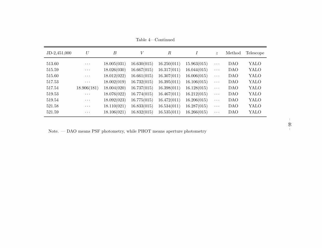
–46

–

Table 4—Continued


513.60 · · · 18.005(031) 16.630(015) 16.250(011) 15.963(015) · · · DAO YALO

515.59 · · · 18.026(030) 16.667(015) 16.317(011) 16.044(015) · · · DAO YALO

515.60 · · · 18.012(022) 16.661(015) 16.307(011) 16.006(015) · · · DAO YALO

517.53 · · · 18.002(019) 16.732(015) 16.395(011) 16.106(015) · · · DAO YALO

517.54 18.906(181) 18.004(020) 16.737(015) 16.398(011) 16.128(015) · · · DAO YALO

519.53 · · · 18.076(022) 16.774(015) 16.467(011) 16.212(015) · · · DAO YALO

519.54 · · · 18.092(023) 16.775(015) 16.472(011) 16.206(015) · · · DAO YALO

521.58 · · · 18.110(021) 16.833(015) 16.534(011) 16.287(015) · · · DAO YALO

521.59 · · · 18.106(021) 16.832(015) 16.535(011) 16.266(015) · · · DAO YALO

Note. — DAO means PSF photometry, while PHOT means aperture photometry

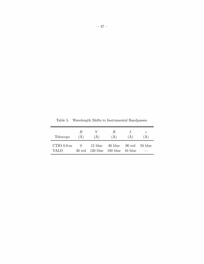
– 47 –

Table 5. Wavelength Shifts to Instrumental Bandpasses

B V R I z

Telescope (A) (A) (A) (A) (A)

CTIO 0.9-m 0 15 blue 30 blue 90 red 50 blue

YALO 30 red 120 blue 180 blue 10 blue · · ·

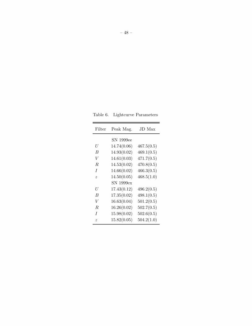
– 48 –

Table 6. Lightcurve Parameters

Filter Peak Mag. JD Max

SN 1999ee

U 14.74(0.06) 467.5(0.5)

B 14.93(0.02) 469.1(0.5)

V 14.61(0.03) 471.7(0.5)

R 14.53(0.02) 470.8(0.5)

I 14.66(0.02) 466.3(0.5)

z 14.50(0.05) 468.5(1.0)

SN 1999ex

U 17.43(0.12) 496.2(0.5)

B 17.35(0.02) 498.1(0.5)

V 16.63(0.04) 501.2(0.5)

R 16.26(0.02) 502.7(0.5)

I 15.98(0.02) 502.6(0.5)

z 15.82(0.05) 504.2(1.0)

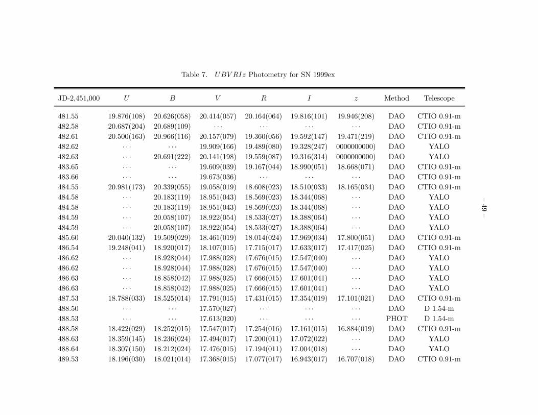
–49

–

Table 7. UBV RIz Photometry for SN 1999ex


481.55 19.876(108) 20.626(058) 20.414(057) 20.164(064) 19.816(101) 19.946(208) DAO CTIO 0.91-m

482.58 20.687(204) 20.689(109) · · · · · · · · · · · · DAO CTIO 0.91-m

482.61 20.500(163) 20.966(116) 20.157(079) 19.360(056) 19.592(147) 19.471(219) DAO CTIO 0.91-m

482.62 · · · · · · 19.909(166) 19.489(080) 19.328(247) 0000000000) DAO YALO

482.63 · · · 20.691(222) 20.141(198) 19.559(087) 19.316(314) 0000000000) DAO YALO

483.65 · · · · · · 19.609(039) 19.167(044) 18.990(051) 18.668(071) DAO CTIO 0.91-m

483.66 · · · · · · 19.673(036) · · · · · · · · · DAO CTIO 0.91-m

484.55 20.981(173) 20.339(055) 19.058(019) 18.608(023) 18.510(033) 18.165(034) DAO CTIO 0.91-m

484.58 · · · 20.183(119) 18.951(043) 18.569(023) 18.344(068) · · · DAO YALO

484.58 · · · 20.183(119) 18.951(043) 18.569(023) 18.344(068) · · · DAO YALO

484.59 · · · 20.058(107) 18.922(054) 18.533(027) 18.388(064) · · · DAO YALO

484.59 · · · 20.058(107) 18.922(054) 18.533(027) 18.388(064) · · · DAO YALO

485.60 20.040(132) 19.509(029) 18.461(019) 18.014(024) 17.969(034) 17.800(051) DAO CTIO 0.91-m

486.54 19.248(041) 18.920(017) 18.107(015) 17.715(017) 17.633(017) 17.417(025) DAO CTIO 0.91-m

486.62 · · · 18.928(044) 17.988(028) 17.676(015) 17.547(040) · · · DAO YALO

486.62 · · · 18.928(044) 17.988(028) 17.676(015) 17.547(040) · · · DAO YALO

486.63 · · · 18.858(042) 17.988(025) 17.666(015) 17.601(041) · · · DAO YALO

486.63 · · · 18.858(042) 17.988(025) 17.666(015) 17.601(041) · · · DAO YALO

487.53 18.788(033) 18.525(014) 17.791(015) 17.431(015) 17.354(019) 17.101(021) DAO CTIO 0.91-m

488.50 · · · · · · 17.570(027) · · · · · · · · · DAO D 1.54-m

488.53 · · · · · · 17.613(020) · · · · · · · · · PHOT D 1.54-m

488.58 18.422(029) 18.252(015) 17.547(017) 17.254(016) 17.161(015) 16.884(019) DAO CTIO 0.91-m

488.63 18.359(145) 18.236(024) 17.494(017) 17.200(011) 17.072(022) · · · DAO YALO

488.64 18.307(150) 18.212(024) 17.476(015) 17.194(011) 17.004(018) · · · DAO YALO

489.53 18.196(030) 18.021(014) 17.368(015) 17.077(017) 16.943(017) 16.707(018) DAO CTIO 0.91-m

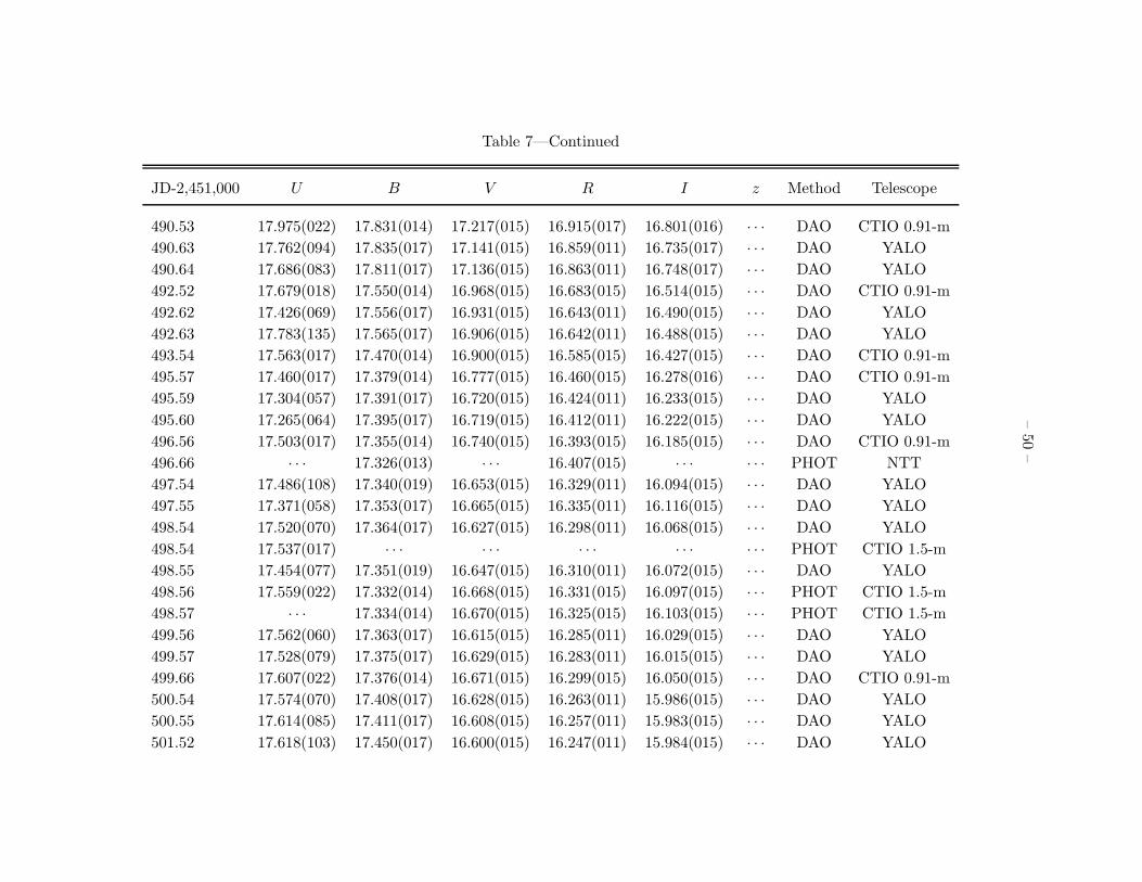
–50

–

Table 7—Continued


490.53 17.975(022) 17.831(014) 17.217(015) 16.915(017) 16.801(016) · · · DAO CTIO 0.91-m

490.63 17.762(094) 17.835(017) 17.141(015) 16.859(011) 16.735(017) · · · DAO YALO

490.64 17.686(083) 17.811(017) 17.136(015) 16.863(011) 16.748(017) · · · DAO YALO

492.52 17.679(018) 17.550(014) 16.968(015) 16.683(015) 16.514(015) · · · DAO CTIO 0.91-m

492.62 17.426(069) 17.556(017) 16.931(015) 16.643(011) 16.490(015) · · · DAO YALO

492.63 17.783(135) 17.565(017) 16.906(015) 16.642(011) 16.488(015) · · · DAO YALO

493.54 17.563(017) 17.470(014) 16.900(015) 16.585(015) 16.427(015) · · · DAO CTIO 0.91-m

495.57 17.460(017) 17.379(014) 16.777(015) 16.460(015) 16.278(016) · · · DAO CTIO 0.91-m

495.59 17.304(057) 17.391(017) 16.720(015) 16.424(011) 16.233(015) · · · DAO YALO

495.60 17.265(064) 17.395(017) 16.719(015) 16.412(011) 16.222(015) · · · DAO YALO

496.56 17.503(017) 17.355(014) 16.740(015) 16.393(015) 16.185(015) · · · DAO CTIO 0.91-m

496.66 · · · 17.326(013) · · · 16.407(015) · · · · · · PHOT NTT

497.54 17.486(108) 17.340(019) 16.653(015) 16.329(011) 16.094(015) · · · DAO YALO

497.55 17.371(058) 17.353(017) 16.665(015) 16.335(011) 16.116(015) · · · DAO YALO

498.54 17.520(070) 17.364(017) 16.627(015) 16.298(011) 16.068(015) · · · DAO YALO

498.54 17.537(017) · · · · · · · · · · · · · · · PHOT CTIO 1.5-m

498.55 17.454(077) 17.351(019) 16.647(015) 16.310(011) 16.072(015) · · · DAO YALO

498.56 17.559(022) 17.332(014) 16.668(015) 16.331(015) 16.097(015) · · · PHOT CTIO 1.5-m

498.57 · · · 17.334(014) 16.670(015) 16.325(015) 16.103(015) · · · PHOT CTIO 1.5-m

499.56 17.562(060) 17.363(017) 16.615(015) 16.285(011) 16.029(015) · · · DAO YALO

499.57 17.528(079) 17.375(017) 16.629(015) 16.283(011) 16.015(015) · · · DAO YALO

499.66 17.607(022) 17.376(014) 16.671(015) 16.299(015) 16.050(015) · · · DAO CTIO 0.91-m

500.54 17.574(070) 17.408(017) 16.628(015) 16.263(011) 15.986(015) · · · DAO YALO

500.55 17.614(085) 17.411(017) 16.608(015) 16.257(011) 15.983(015) · · · DAO YALO

501.52 17.618(103) 17.450(017) 16.600(015) 16.247(011) 15.984(015) · · · DAO YALO

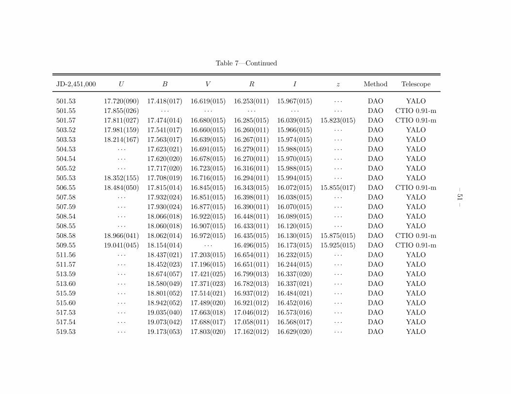
–51

–

Table 7—Continued


501.53 17.720(090) 17.418(017) 16.619(015) 16.253(011) 15.967(015) · · · DAO YALO

501.55 17.855(026) · · · · · · · · · · · · · · · DAO CTIO 0.91-m

501.57 17.811(027) 17.474(014) 16.680(015) 16.285(015) 16.039(015) 15.823(015) DAO CTIO 0.91-m

503.52 17.981(159) 17.541(017) 16.660(015) 16.260(011) 15.966(015) · · · DAO YALO

503.53 18.214(167) 17.563(017) 16.639(015) 16.267(011) 15.974(015) · · · DAO YALO

504.53 · · · 17.623(021) 16.691(015) 16.279(011) 15.988(015) · · · DAO YALO

504.54 · · · 17.620(020) 16.678(015) 16.270(011) 15.970(015) · · · DAO YALO

505.52 · · · 17.717(020) 16.723(015) 16.316(011) 15.988(015) · · · DAO YALO

505.53 18.352(155) 17.708(019) 16.716(015) 16.294(011) 15.994(015) · · · DAO YALO

506.55 18.484(050) 17.815(014) 16.845(015) 16.343(015) 16.072(015) 15.855(017) DAO CTIO 0.91-m

507.58 · · · 17.932(024) 16.851(015) 16.398(011) 16.038(015) · · · DAO YALO

507.59 · · · 17.930(024) 16.877(015) 16.390(011) 16.070(015) · · · DAO YALO

508.54 · · · 18.066(018) 16.922(015) 16.448(011) 16.089(015) · · · DAO YALO

508.55 · · · 18.060(018) 16.907(015) 16.433(011) 16.120(015) · · · DAO YALO

508.58 18.966(041) 18.062(014) 16.972(015) 16.435(015) 16.130(015) 15.875(015) DAO CTIO 0.91-m

509.55 19.041(045) 18.154(014) · · · 16.496(015) 16.173(015) 15.925(015) DAO CTIO 0.91-m

511.56 · · · 18.437(021) 17.203(015) 16.654(011) 16.232(015) · · · DAO YALO

511.57 · · · 18.452(023) 17.196(015) 16.651(011) 16.244(015) · · · DAO YALO

513.59 · · · 18.674(057) 17.421(025) 16.799(013) 16.337(020) · · · DAO YALO

513.60 · · · 18.580(049) 17.371(023) 16.782(013) 16.337(021) · · · DAO YALO

515.59 · · · 18.801(052) 17.514(021) 16.937(012) 16.484(021) · · · DAO YALO

515.60 · · · 18.942(052) 17.489(020) 16.921(012) 16.452(016) · · · DAO YALO

517.53 · · · 19.035(040) 17.663(018) 17.046(012) 16.573(016) · · · DAO YALO

517.54 · · · 19.073(042) 17.688(017) 17.058(011) 16.568(017) · · · DAO YALO

519.53 · · · 19.173(053) 17.803(020) 17.162(012) 16.629(020) · · · DAO YALO

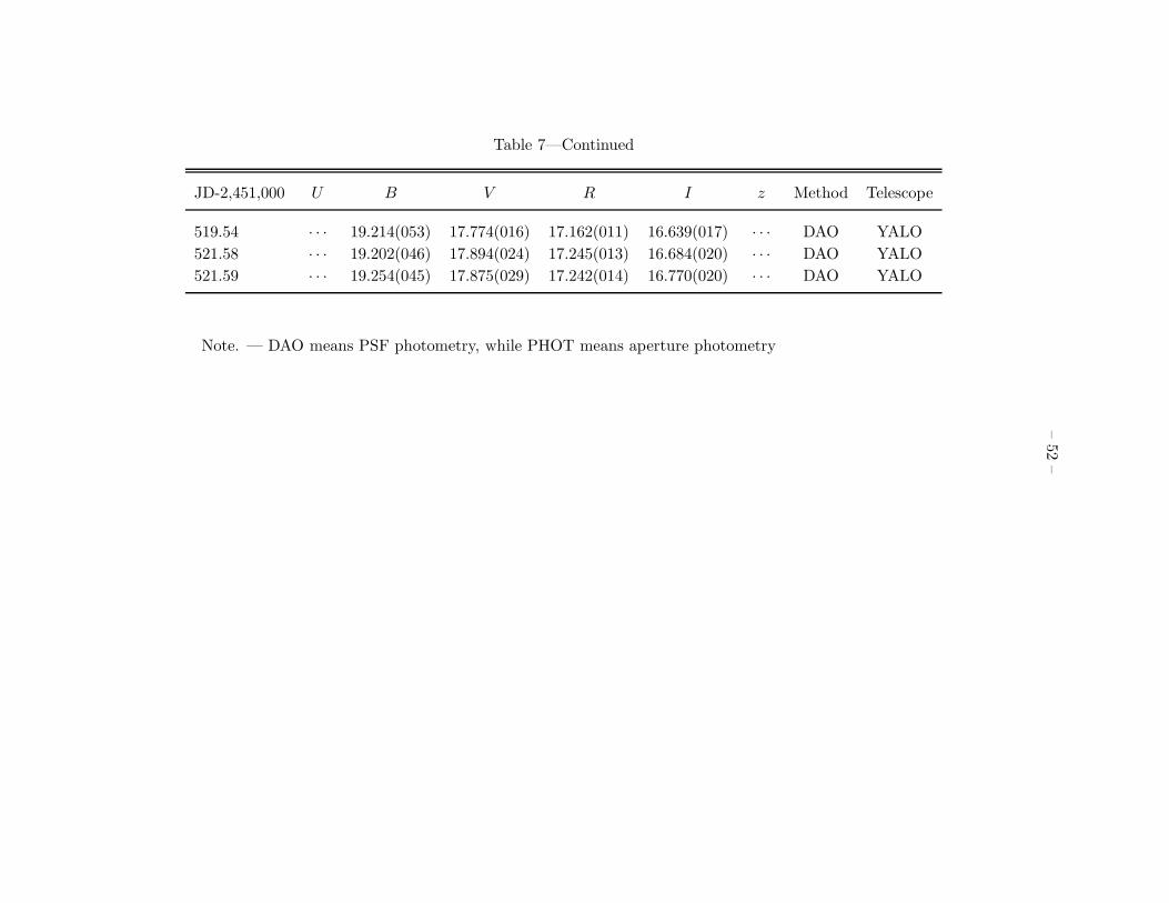
–52

–

Table 7—Continued


519.54 · · · 19.214(053) 17.774(016) 17.162(011) 16.639(017) · · · DAO YALO

521.58 · · · 19.202(046) 17.894(024) 17.245(013) 16.684(020) · · · DAO YALO

521.59 · · · 19.254(045) 17.875(029) 17.242(014) 16.770(020) · · · DAO YALO

Note. — DAO means PSF photometry, while PHOT means aperture photometry

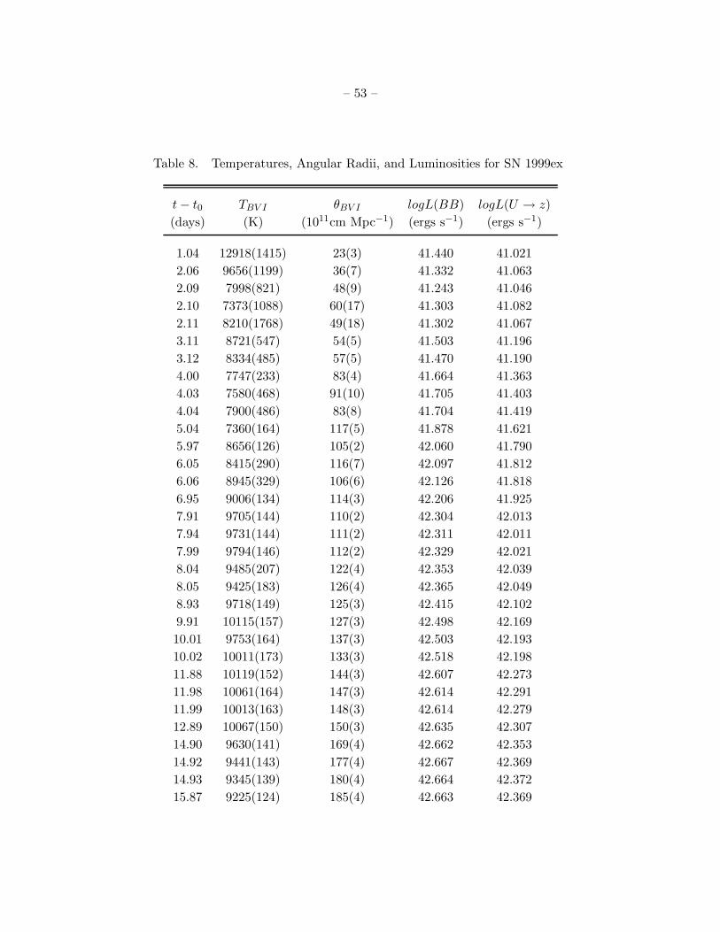
– 53 –

Table 8. Temperatures, Angular Radii, and Luminosities for SN 1999ex

t − t0 TBV I θBV I logL(BB) logL(U → z)

(days) (K) (1011cm Mpc−1) (ergs s−1) (ergs s−1)

1.04 12918(1415) 23(3) 41.440 41.021

2.06 9656(1199) 36(7) 41.332 41.063

2.09 7998(821) 48(9) 41.243 41.046

2.10 7373(1088) 60(17) 41.303 41.082

2.11 8210(1768) 49(18) 41.302 41.067

3.11 8721(547) 54(5) 41.503 41.196

3.12 8334(485) 57(5) 41.470 41.190

4.00 7747(233) 83(4) 41.664 41.363

4.03 7580(468) 91(10) 41.705 41.403

4.04 7900(486) 83(8) 41.704 41.419

5.04 7360(164) 117(5) 41.878 41.621

5.97 8656(126) 105(2) 42.060 41.790

6.05 8415(290) 116(7) 42.097 41.812

6.06 8945(329) 106(6) 42.126 41.818

6.95 9006(134) 114(3) 42.206 41.925

7.91 9705(144) 110(2) 42.304 42.013

7.94 9731(144) 111(2) 42.311 42.011

7.99 9794(146) 112(2) 42.329 42.021

8.04 9485(207) 122(4) 42.353 42.039

8.05 9425(183) 126(4) 42.365 42.049

8.93 9718(149) 125(3) 42.415 42.102

9.91 10115(157) 127(3) 42.498 42.169

10.01 9753(164) 137(3) 42.503 42.193

10.02 10011(173) 133(3) 42.518 42.198

11.88 10119(152) 144(3) 42.607 42.273

11.98 10061(164) 147(3) 42.614 42.291

11.99 10013(163) 148(3) 42.614 42.279

12.89 10067(150) 150(3) 42.635 42.307

14.90 9630(141) 169(4) 42.662 42.353

14.92 9441(143) 177(4) 42.667 42.369

14.93 9345(139) 180(4) 42.664 42.372

15.87 9225(124) 185(4) 42.663 42.369

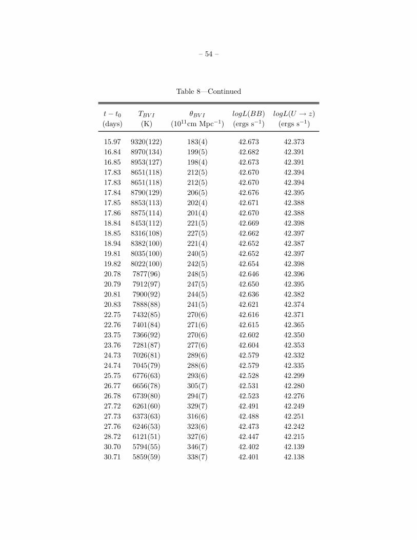
– 54 –

Table 8—Continued



15.97 9320(122) 183(4) 42.673 42.373

16.84 8970(134) 199(5) 42.682 42.391

16.85 8953(127) 198(4) 42.673 42.391

17.83 8651(118) 212(5) 42.670 42.394

17.83 8651(118) 212(5) 42.670 42.394

17.84 8790(129) 206(5) 42.676 42.395

17.85 8853(113) 202(4) 42.671 42.388

17.86 8875(114) 201(4) 42.670 42.388

18.84 8453(112) 221(5) 42.669 42.398

18.85 8316(108) 227(5) 42.662 42.397

18.94 8382(100) 221(4) 42.652 42.387

19.81 8035(100) 240(5) 42.652 42.397

19.82 8022(100) 242(5) 42.654 42.398

20.78 7877(96) 248(5) 42.646 42.396

20.79 7912(97) 247(5) 42.650 42.395

20.81 7900(92) 244(5) 42.636 42.382

20.83 7888(88) 241(5) 42.621 42.374

22.75 7432(85) 270(6) 42.616 42.371

22.76 7401(84) 271(6) 42.615 42.365

23.75 7366(92) 270(6) 42.602 42.350

23.76 7281(87) 277(6) 42.604 42.353

24.73 7026(81) 289(6) 42.579 42.332

24.74 7045(79) 288(6) 42.579 42.335

25.75 6776(63) 293(6) 42.528 42.299

26.77 6656(78) 305(7) 42.531 42.280

26.78 6739(80) 294(7) 42.523 42.276

27.72 6261(60) 329(7) 42.491 42.249

27.73 6373(63) 316(6) 42.488 42.251

27.76 6246(53) 323(6) 42.473 42.242

28.72 6121(51) 327(6) 42.447 42.215

30.70 5794(55) 346(7) 42.402 42.139

30.71 5859(59) 338(7) 42.401 42.138

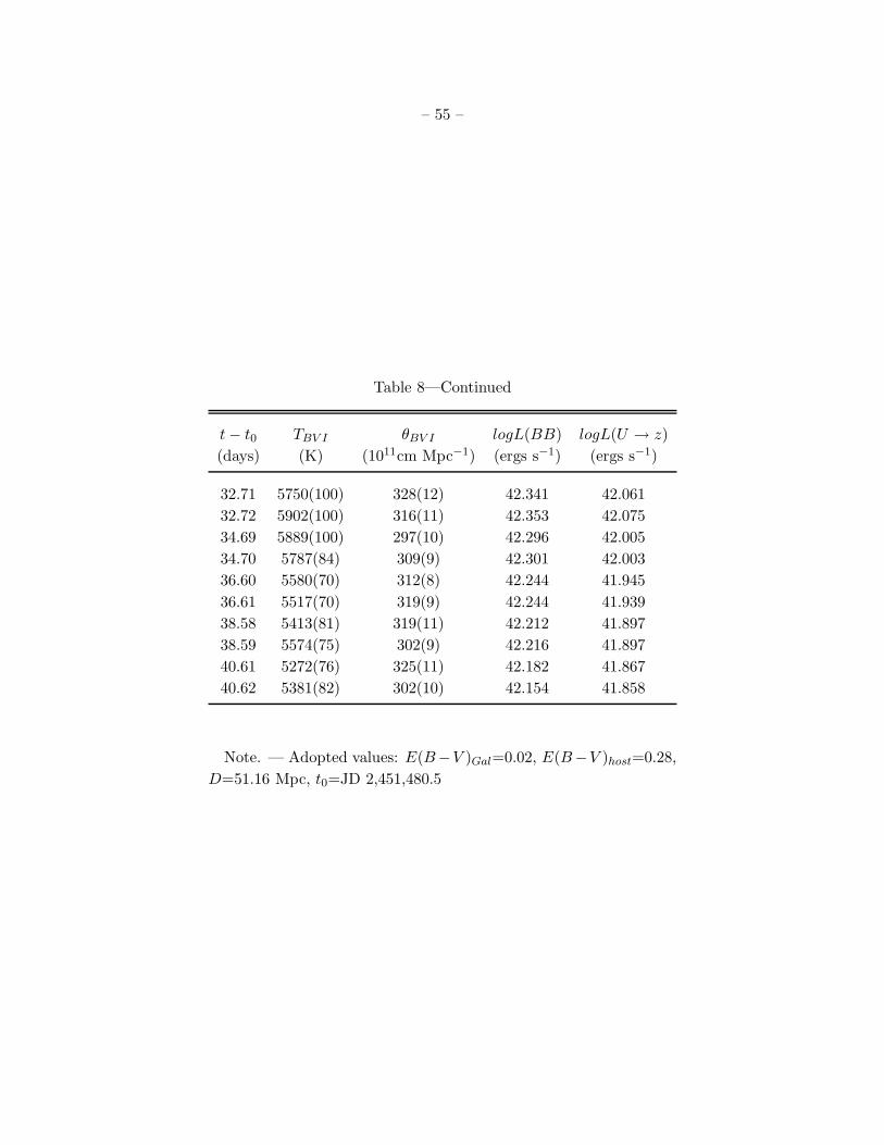
– 55 –

Table 8—Continued



32.71 5750(100) 328(12) 42.341 42.061

32.72 5902(100) 316(11) 42.353 42.075

34.69 5889(100) 297(10) 42.296 42.005

34.70 5787(84) 309(9) 42.301 42.003

36.60 5580(70) 312(8) 42.244 41.945

36.61 5517(70) 319(9) 42.244 41.939

38.58 5413(81) 319(11) 42.212 41.897

38.59 5574(75) 302(9) 42.216 41.897

40.61 5272(76) 325(11) 42.182 41.867

40.62 5381(82) 302(10) 42.154 41.858

Note. — Adopted values: E(B−V )Gal=0.02, E(B−V )host=0.28,

D=51.16 Mpc, t0=JD 2,451,480.5

Optical Photometry of the Type Ia SN 1999ee and the Type Ib/c SN 1999ex in IC 5179

Documents