Optical Depth Sensor for the measurement of dust and ...

- 1 -

Thèse de doctorat de l’Université Versailles Saint-Quentin-en-Yvelines

Spécialité : Astrophysique

Présentée par

Trần Thế Trung

pour obtenir le grade de DOCTEUR de l’Université Versailles Saint-Quentin-en-Yvelines

Optical Depth Sensor for the measurement of dust and clouds in the atmosphere of Mars. Radiative transfer simulations and

validation on Earth.

Soutenance prévue le 20 Décembre 2005 Devant le jury composé de:

M. Gilles Bergametti Rapporteur M. Gerard Brogniez Rapporteur M. Jean-Pierre Pommereau Directeur de Thèse M. Rannou Pascal Co-directeur/Examinateur M. Hervé de Féraudy Président M. Francois Forget Invité M. Quang Rieu Nguyen Invité

- 2 -

- 3 -

Table of Contents Table of Contents ....................................................................................................................... 3 Acknowledgements .................................................................................................................... 5 Introduction ................................................................................................................................ 6

General scientific objectives .................................................................................................. 6 The ODS instrument............................................................................................................... 6 My role in the project ............................................................................................................. 7 Presentation of the thesis........................................................................................................ 7

Chapter 2 .................................................................................................................................... 9 Mars atmosphere and the Optical Depth Sensor ........................................................................ 9

2.1 Introduction ...................................................................................................................... 9 2.2 Scientific background - Martian atmosphere and meteorology ....................................... 9

2.2.1 History of Observations............................................................................................. 9 2.2.2 Current knowledge of Martian meteorology ........................................................... 10 2.2.3 Conclusion............................................................................................................... 12

2.3 Attempts for deploying a meteorological network on Mars........................................... 12 2.3.1 Mars96 mission ....................................................................................................... 13 2.3.2 The NETLANDER mission .................................................................................... 14 2.3.3 The Pascal mission .................................................................................................. 14

2.4 Scientific concept of ODS.............................................................................................. 14 2.4.1 Aerosol optical measurement principle of ODS...................................................... 15 2.4.2 Cloud observation principle of ODS ....................................................................... 15 2.4.3 Design principle ...................................................................................................... 16

2.5 Design and description of NETLANDER prototype ..................................................... 16 2.5.1 Re-designs from Mars96 version ............................................................................ 16 2.5.2 Optical head............................................................................................................. 17 2.5.3 Electronics ............................................................................................................... 17

2.6 Technical development and validation........................................................................... 18 2.6.1 Overview of technical development of ODS .......................................................... 18 2.6.2 ODS field of view characterization ......................................................................... 18

2.7 Conclusion...................................................................................................................... 22 Chapter 3 .................................................................................................................................. 23 Models of radiative transfer in spherical atmosphere .............................................................. 23

3.1 Introduction .................................................................................................................... 23 3.2 Radiative transfer equations ........................................................................................... 23 3.3 Description of the Monte-Carlo model .......................................................................... 24

3.3.1 The principle of the Monte-Carlo approach ............................................................ 24 3.3.2 Monte-Carlo model in a parallel-plane atmosphere ................................................ 25 3.3.3 Detailed description of the Monte-Carlo in spherical geometry ............................. 27

3.4 SHDOM in spherical atmosphere................................................................................... 30 3.4.1 Principle of the SHDOM approach ......................................................................... 30 3.4.2 Description of the delta method for the SHDOM ................................................... 34 3.4.3 SHDOM in spherical geometry............................................................................... 37 3.4.4 Input to simulation................................................................................................... 40 3.4.5 Details of simulation ............................................................................................... 40 3.4.6 Output of the code ................................................................................................... 42

3.5 Validations and comparisons.......................................................................................... 42 3.5.1 Comparison with single scattering solutions........................................................... 42

- 4 -

3.5.2 Multiple scattering mode......................................................................................... 45 3.5.3 Validation by solution of statistical mechanics....................................................... 47 3.5.4 Comparisons............................................................................................................ 49

3.6 Conclusions .................................................................................................................... 56 Chapter 4 .................................................................................................................................. 57 Simulation of ODS measurements on Mars ............................................................................. 57

4.1 Introduction .................................................................................................................... 57 4.2 Daytime dust measurements........................................................................................... 57

4.2.1 Simulation of measurements ................................................................................... 57 4.2.2 Retrieval procedure ................................................................................................. 60 4.2.3 Applications............................................................................................................. 62 4.2.4 Conclusions ............................................................................................................. 65

4.3 Cloud detection at twilight ............................................................................................. 66 4.3.1 Simulation of cloud signature.................................................................................. 66 4.3.2 Retrieval procedure ................................................................................................. 70 4.3.3 Applications............................................................................................................. 71 4.3.4 Conclusions ............................................................................................................. 72

4.4 Conclusions .................................................................................................................... 72 Chapter 5 .................................................................................................................................. 74 Validation of ODS on the Earth ............................................................................................... 74

5.1 Introduction .................................................................................................................... 74 5.2 ODS scientific models.................................................................................................... 74

5.2.1 Experimental setup .................................................................................................. 74 5.2.2 Desert dust and cirrus clouds at the tropics............................................................. 75

5.3 Experimental results ....................................................................................................... 76 5.4 Data analysis................................................................................................................... 78

5.4.1 ODS orientation....................................................................................................... 78 5.4.2 Dust ......................................................................................................................... 81 5.4.3 Cirrus clouds............................................................................................................ 87

5.5 Suggestions for an ODS terrestrial version .................................................................... 91 5.6 Conclusion...................................................................................................................... 92

General Conclusion .................................................................................................................. 93 Appendix .................................................................................................................................. 95

Appendix 1 ........................................................................................................................... 95 Appendix 2 ........................................................................................................................... 95 Appendix 3 ........................................................................................................................... 95 Appendix 4 ........................................................................................................................... 96

References ................................................................................................................................ 98

- 5 -

Acknowledgements

I own the ideas of the studied subject to professor Jean-Pierre Pommereau, the principle investigator of ODS instrument. His rich instrumental experience and knowledge in the

meteorological study of terrestrial atmosphere has partially been transferred to many results of the study.

I would like to express my deep gratitude to professor Pascal Rannou, my co-director during the three years of this Ph.D. study as well as my director in M.Sc. training course. Professor

Pascal helped me to obtain a scholarship from University of Versailles. He stands by my side in searching accommodation and preparing visa during my return to France at the beginning

of the study and several times during my stay in France. My research experience at the Service d'Aeronomie is constantly powered by professor’s guiding and encouraging

comments, usually with humors.

My study in France would not be possible without the help of professor Nguyen Quang Rieu, who desire has been always to form a group of young astrophysicists for Vietnam.

As said, the thesis is funded by the University of Versailles. I also acknowledge the financial

support of Centre National d'Études Spatiales, France, for the NETLANDER project.

Research is a community business. I would like to thank the ODS team, Jean-Luc Maria, Christian Malique, Jean-Jacques Correia, Jacques Porteneuve, for the joy time we have spent together in developing the instrument from initial conception to today’s working prototype.

I am helped by many scientific colleagues and administrators inside and outside Service

d'Aeronomie.

Finally, I pay my special thanks to family and friends, in France and at distance parts of the world, for their constant encourages.

- 6 -

Introduction

General scientific objectives One thing is clear, human being will not cease its exploration of the universe. Mars, the planet that offers best habitable conditions for terrestrial life than all other solar system planets after the Earth, is not only a candidate for our extraterrestrial terraforming ambition but also a natural laboratory for our knowledge expansion, and the better understanding of worlds other than our homeland. The discoveries made in the study of Martian atmosphere, in particular, are important parts of our exploration of Mars. Today, we know that this atmosphere is unique in the solar system, dry and dusty, with the characteristics for a great desert. Intriguingly, both Mars and Earth are expected to have similar atmospheric composition at their early stages of formation. The divergence of atmospheric evolutions teaches us lessons on how process such as run-away green house effect could dramatically change the global climatology in un-recoverable ways. The better knowledge of Mars and its atmosphere requires observations; most of these are now coming from scientific missions sent to the red planet. Those missions are performing both remote sensing from orbit and in-situ measurements at the surface. They are providing crucial data for refining the physical model of the planet. In the case of Martian atmosphere modelling, two important parameters that are needed to be monitored by in-situ measurements are the amount of dust loading in atmosphere and the circulation of Martian water ice clouds. Indeed, we know that the atmosphere is constantly charged with fine ferrite dust blew up from the surface by winds. These dust loadings play a crucial role in controlling Martian atmospheric vertical structure. Understanding the meteorology requires a model on the amount of dust in the atmosphere. Yet, modelling of dust loading remains difficult, because of the many unknowns in the lifting mechanisms. An efficient approach forgetting more information on the subject would be in situ measurements with instruments deposited at the surface of the planet. Another modelling that also requires constraints from in-situ measurements is the circulation of water vapour. Normally, water ice cirrus are extremely thin and hard to detect. Further requirements on the measurements are a wide coverage to obtain global patterns, and a long duration to capture seasonal and inter-annual variability. Within the general limits of spatial missions to the red planet, (for example in energy resource and data transmissions), such monitoring may be best accomplished by a network of light-weight, energy-saving and low data rate instruments, placed over critical points of the surface and operating for several years. A potential instrument for such network is ODS.

The ODS instrument ODS, Optical Depth Sensor, has been designed to meet with all above technical and scientific requirements providing daily measurements of both dust optical thickness and high altitude ice clouds. The optical depth is derived from alternative observations of sunlight scattered at zenith and direct sunlight when the sun passes within the field of view. The presence of clouds is detected by looking at the evolution of the color of the sky during twilight using two spectral channels in the blue and red. Dust and cloud properties are retrieved using radiative transfer simulations.

- 7 -

ODS has been developed at the Service d’Aéronomie for previous missions to Mars. The instrument was first chosen for the meteorological package of the Russian mission MARS96 which fell in the Pacific. In a lighter design it was proposed to the NASA PASCAL Mars meteorological network but which was finally abandoned. At last a new version including a deep modification and simplification of the optics has been studied in 2002-2004 for the new CNES NETLANDER mission. The work has included the manufacturing and testing of several prototypes as well as the development of a mathematical radiative transfer model for adjusting at best the optical set-up and preparing the data retrieval. Furthermore several scientific versions of the instrument have been manufactured for validation of both the principle of the measurements and the retrieval procedure during field campaigns on the Earth. The project was approaching the end of the space phase B study when unfortunately the NETLANDER mission was cancelled in spring 2004. The work described in this thesis is that carried during the development of the NETLANDER ODS instrument as well as during its further scientific validation, which was continued though the Mars project was stopped. The validation includes side by side comparisons with the well established AERONET aerosol photometer in a desert dust region in West Africa carried in 2004-2005. An important outcome of the validation exercise in Africa, is the demonstration of the ability of the ODS technique to detect high altitude thin cirrus around the tropopause, which could be hardly observed by other methods. Thin cirrus are key elements of the Earth atmosphere in the tropics. They could play a significant role in controlling the amount of water vapour entering in the stratosphere as well as depending on the optical thickness, on radiative transfer and thus climate. Their study is therefore a priority of the new coming AMMA and SCOUT projects in Africa. It is thus not surprising that the ODS measurements have received immediate application. The decision was made to leave the prototype operating for the AMMA period in 2006 at Ouagadougou in Burkina Faso, which will be completed by the deployment of two additional instruments at Tamanrasset in South Algeria and Niamey in Niger, both next to lidar systems. Although all efforts are still given to deploy ODS on Mars, e.g. on the ESA Exo-Mars mission in 2011, the African projects offer a unique opportunity of significant scientific return of the effort committed to the development of the instrument during the last three years.

My role in the project My contribution to project has been: a) the development of radiative transfer models, first a full Monte-Carlo code in spherical geometry, then a fast modified SHDOM for spherical geometry validated by comparison with the first; b) the simulation of ODS dust optical thickness and clouds measurements on Mars, c) the use of the model for adjusting and improving the design and validating the NETLANDER prototype; and, d) the analysis of the measurements in Africa, their comparison to those of the AERONET photometer and the detection of cirrus clouds at the tropopause.

Presentation of the thesis After this first chapter of introduction, the thesis is organised as follows. Chapter 2 provides the background information on Mars meteorology, on the role of dust and clouds, the concept of ODS for monitoring them from surface stations, the previous attempts

- 8 -

to deploy the instrument on the planet and finally a description of the NETLANDER prototype needed to define the requirements of the modelling. Chapter 3, is a detailed description of the radiative transfer models developed for simulating ODS measurements in spherical geometry, mandatory for capturing twilight observations. Two models will be used. First, accurate but slow Monte-Carlo calculations and then lighter SHDOM (Spherical Harmonics Discrete Ordinates) calculations modified for spherical geometry which will be compared to the first. Chapter 4 presents the results of the simulations of the ODS measurements used for checking the instrument sensitivity to dust and cloud properties, defining the retrieval process and optimizing the ODS design (FOV, filters, sampling rate, etc.). Chapter 5 describes the results of the validation campaigns in Africa, including the comparison to the optical depth measurements of the AERONET photometer and preliminary results on the detection cirrus clouds near the tropopause. Chapter 6 provides the overall conclusions.

- 9 -

Chapter 2

Mars atmosphere and the Optical Depth Sensor

2.1 Introduction The objective of the thesis is the definition and validation of a light instrument for long term daily monitoring of Martian dust and water ice cloud opacity, some of the most important meteorological parameters of Mars, from small stations deployed at the surface of the planet, during the NETLANDER mission. After a brief description of the scientific background and the importance of dust and water ice cloud in the meteorology of Mars, the chapter will describe the concept of the ODS instrument for measuring those parameters. It will then mention the unfortunate previous attempts for deploying ODS on Mars and will provide a description of the ODS current version adopted for the NETLANDER mission.

2.2 Scientific background - Martian atmosphere and meteorology

2.2.1 History of Observations Since the first observations, Mars always appears as an alien world with yet many familiar characteristics. In the late 19th century, telescopic observation techniques had difficulty distinguishing Martian surface features. Lighter or darker albedo features were believed to be oceans and continents. Mars also was believed to have a relatively substantial atmosphere. Astronomers knew that the rotation period of Mars (the length of its day) was almost the same as that of the Earth, as well as its inclination, which meant it had seasons. Mars polar ice caps were also observed to shrink and grow with the changing seasons. These changes were interpreted as being due to the seasonal growth of plant life. From the Lowell Observatory, Percival Lowell observations of “Martian canals” went as far as suggesting an irrigation network on the surface (Wallace 1907). By the late 1920s, however, it was known that Mars was very dry and had a very low pressure atmosphere of almost pure carbon dioxide. The first pictures revealing impact craters and a generally barren landscape were obtained by the arrival of the space probe Mariner 4 in 1965. Mars appeared to be the biggest desert in solar system with unique feature of constant atmospheric suspended ferrite dust layers. Then Mariner 9 showed heavy dust loading and ice haze as well as spectral signal of water-ice cirrus on Mars (Anderson and Leovy 1977). Viking Landers from 1976 to 1982 revealed an atmospheric structure containing both troposphere and stratosphere with clouds layers at transitional altitudes. In the past decade, a series of international missions to Mars has brought an exponential growing scientific data set about the planet, including some recent remarkable discoveries such as the strong evidence of ancient Martian water abundance, the possible current sub-surface water ice reservoir and the signature of the intriguing organic gas CH4 in local atmospheric region, first observed in 2003 by telescopic spectral analysis (Krasnopolsky et al 2004).

- 10 -

2.2.2 Current knowledge of Martian meteorology Current observations suggest a unique dynamic of Martian meteorology. Mars, from a meteorological point of view, is the largest desert in the Solar system. The vertical structure of the atmosphere also has a troposphere and a stratosphere, where most of weather activities occur in the troposphere (Figure II.1). The troposphere constantly has a dust layer lifted by strong winds, despite the relatively low atmospheric density. The temperature profile and the cloud structure are quite different from the terrestrial case, due to some unique meteorological processes.

Figure II.1 Comparison between Martian and Terrestrial atmospheric vertical structures. There are two main factors that control the vertical structure of the lower atmosphere, pressure and dust. Carbon dioxide, the major component of the atmosphere, radiates efficiently at cold Martian temperature and pressure, causing the atmosphere to respond rapidly to changes in the amount of solar radiation received. Suspended dust absorbs large quantities of heat directly from sunlight and provides a distributed energy source throughout the lower atmosphere. Atmospheric dust strongly affects the meteorology of Mars (Gierasch and Goody 1972, Haberle et al. 1982). In particular, as shown on Figure II.2 (extracted from the thesis of Françoise Forget, University Paris 6, 1996), the temperature profile can vary largely with the dust loading. This is because dust is the main absorber and scatterer of the atmosphere at visible wavelengths. Therefore it plays a crucial role in the global radiation budget of the planet. Temperatures depend on latitude and fluctuate over a wide diurnal and seasonal range, much larger than in desert regions on the Earth. The large diurnal cycle is due to a relatively thin atmosphere that could not insulate the ground from outer space and the lack of oceans that have a large thermal inertia. Temperature and pressure oscillations, sometimes called tides, can appear throughout the atmosphere as a result of the direct input of solar energy. They are regular, periodic, and synchronized with the position of the Sun. Large seasonal variation of Martian temperature in turn changes the atmospheric carbon dioxide pressure through seasonal deposition and release of a large fraction of the Martian atmosphere (forming and melting of polar caps). Daily temperature swing depends on atmospheric dust loading and reduces during dust storms, thanks to dust heat distribution. The large amount of suspended

- 11 -

dust is also thought to be responsible for a relatively high tropopause and near constant temperature profile of the stratosphere.

Figure II.2 Temperature profile of the Martian atmosphere as function of altitude for different dust optical depths. Turbulence and wind are an important factor in injecting and maintaining the large quantity of dust found in the atmosphere. However, dust lifting mechanisms remain little understood, partly because of lack of measurements of wind speed. Dust storms tend to begin at preferred locations in the southern hemisphere during southern spring and summer. However, it is not understood how local scale activity could result in large amounts of dust high into the atmosphere. If the amount of dust reaches a critical quantity, the storm rapidly intensifies, and dust is carried by high winds to all parts of the planet. This leads in a few days to a global obscuration of the surface, with visible optical depth reaching 4 or more. The intensification process is evidently short-lived, as atmospheric opacity begins to decline almost immediately, returning to normal in a few weeks. Apart from dust and carbon dioxide, water, despite being a minor constituent of the atmosphere, plays an important role in atmospheric chemistry and meteorology. The atmosphere is effectively saturated with water vapour, yet under cold temperature and pressure, water molecules can exist only as ice or vapour, giving rise to Earth-like frost and large cirrus clouds of water ice. Water vapour is found uniformly mixed up to 10 -15 km and shows strong latitudinal gradients that depend on the season. It has a global dynamic, moving from North Pole to the whole globe at spring, and returning to the pole at fall (Haberle and Jakosky 1990). The atmospheric water vapour concentration is now believed to be controlled by a much larger reservoir in the Martian soil (undergoing little daily exchange with the surface). This means the water ice clouds are tracers of water and in turn, impact its global distribution (Clancy et al. 1996, James 1990). Cloud opacity is directly linked to the atmospheric water content and results in a strong constraint on the understanding of water cycle. Observation of water vapor transport also places a constraint on global wind circulation.

- 12 -

Current observations of Martian meteorology combined with various theoretical projections provide some general ideals of the evolution of the meteorology. The ratio of carbon dioxide and molecular nitrogen relative to that of the trace gases is about 10 times smaller on Mars than on the Earth. This is interpreted, by photochemical reactions at the top of the atmosphere, as an indication that Mars has lost large amounts of carbon dioxide and molecular nitrogen during its history. It is further conjectured, on the basis of these ideas, that Mars may once have had an atmosphere of carbon dioxide, molecular nitrogen, and water in quantities similar to those found on early Earth and Venus. This includes the idea that warm wet conditions prevailed at an early stage of evolution. The smaller mass and further distance to the Sun are among the most important factors that may contribute to evolution of the atmosphere, much different from the terrestrial case. Observations such as the existence of possible dried river network support the conjecture on Martian ancient water abundance. However the details of evolution scenario need be confirmed by future observations.

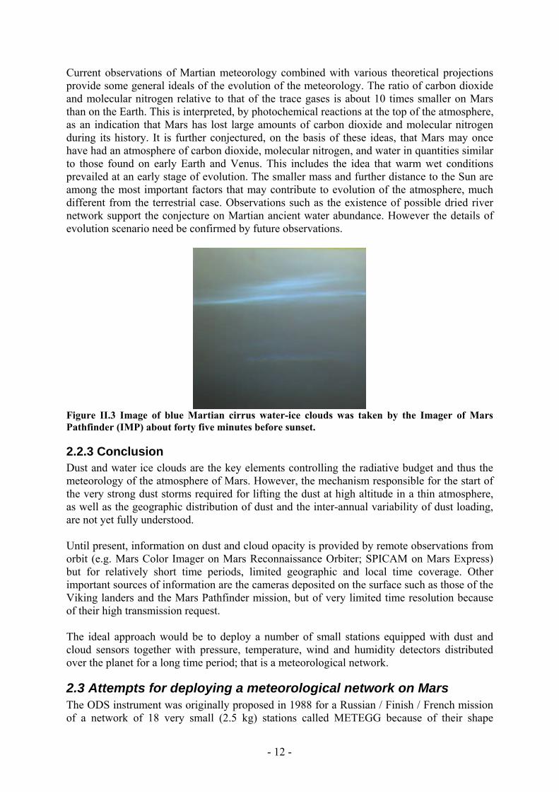
Figure II.3 Image of blue Martian cirrus water-ice clouds was taken by the Imager of Mars Pathfinder (IMP) about forty five minutes before sunset.

2.2.3 Conclusion Dust and water ice clouds are the key elements controlling the radiative budget and thus the meteorology of the atmosphere of Mars. However, the mechanism responsible for the start of the very strong dust storms required for lifting the dust at high altitude in a thin atmosphere, as well as the geographic distribution of dust and the inter-annual variability of dust loading, are not yet fully understood. Until present, information on dust and cloud opacity is provided by remote observations from orbit (e.g. Mars Color Imager on Mars Reconnaissance Orbiter; SPICAM on Mars Express) but for relatively short time periods, limited geographic and local time coverage. Other important sources of information are the cameras deposited on the surface such as those of the Viking landers and the Mars Pathfinder mission, but of very limited time resolution because of their high transmission request. The ideal approach would be to deploy a number of small stations equipped with dust and cloud sensors together with pressure, temperature, wind and humidity detectors distributed over the planet for a long time period; that is a meteorological network.

2.3 Attempts for deploying a meteorological network on Mars The ODS instrument was originally proposed in 1988 for a Russian / Finish / French mission of a network of 18 very small (2.5 kg) stations called METEGG because of their shape

- 13 -

designed to allow their automatic orientation to the zenith after landing. However because of the need to host other instruments such as a seismometer, a magnetometer etc, the stations became heavier and their number was reduced to 4 and then to 2 for economic reasons for the Russian MARS96 mission, but which finally dropped into the Pacific a little after launch. The second attempt in which ODS was also involved, was the PASCAL network proposed by the NASA-AMES center for the SCOUT mission, but which has been finally not selected in 2003. The third attempt was the CNES European NETLANDER mission of 4 stations planned for 2007, for which ODS has been re-designed, but which was stopped in spring 2003. Before describing the most recent NETLANDER ODS version we will briefly summarize the information of the previous attempts.

2.3.1 Mars96 mission ODS was first built for the Russian mission MARS96. MARS96 was an ambitious mission, which main scientific objectives were to investigate the evolution of Mars, that is, of its atmosphere, its surface, and its interior by using various, global-scale and comprehensive methods (Likin et al., 1998). The MARS-96 spacecraft consisted of an orbiter, two autonomous small stations to land on the surface and two penetrators to enter into the Martian soil. During the cruise phase from Earth to Mars, additional astrophysical observations of interplanetary space parameters were to be conducted. This mission was one of the highest priorities of Russian Federation Space Studies Program. It was mostly designed and manufactured by Russian institutes, with collaborations from many European and American laboratories. The program started in 1989 and the spacecraft was launched from Baikonur, Russia, on 16 November 1996 but unfortunately could not reached interplanetary trajectory to Mars due to a malfunction in the third stage of the rocket and fell back into the Pacific Ocean. The Mars-96 scientific experiments were to explore the following problems:

1. The Mars surface: a global topographic survey of the surface including local high-resolution studies of terrain; mineralogical mapping; elemental composition of the soil; studies of the cryolithozone and its deep structure.

2. The atmosphere and climatic monitoring of the planet: studies of the Martian climate; abundance of minor components in the atmosphere (H2O, CO, O3 , etc), their variation and vertical distribution, and searches for regions with higher humidity; global monitoring of the 3D atmospheric temperature distribution; pressure variations over spatial and time domains; characterization of the atmosphere near the volcanic mountains; characteristics of atmospheric aerosols; neutral and ion composition of the upper atmosphere.

3. The inner structure of the planet: crust thickness; magnetic field; thermal flux; search for active volcanoes; seismic activity.

4. Plasma: parameters of the Martian magnetic field: its momentum and orientation; the 3D distribution function; the ion and energy composition of plasma (near Mars and during interplanetary cruise); plasma wave characteristics (electric and magnetic fields); the structure of the magnetosphere and its boundaries.

5. Astrophysical studies: localization of cosmic gamma-bursts; oscillations of stars and the Sun.

ODS was part of the meteorological package of the two landers. The ODS instrument was based on the same concept but of different arrangement of the current version. It was a four spectral channel instruments (350, 550 and 750 nm for dust opacity and 270 nm for ozone), oriented to the zenith with a 50° FOV. The optical set up using a lens and optical fibers, also

- 14 -

include an annular mask to look alternatively at sunlight scattered at zenith and at the sum of direct and scattered sunlight. In this version, ODS was weighting 355g (115g for the optical system on the top of the station and 240g electronics in the warmer inside). The principle of this system for measuring dust has been validated on the Earth in a Martian analog environment in the Sahelian region at Ouagadougou in Burkina Faso (Ph.D. thesis of Thierry Carpentier, Université Paris 6, 1996). Unfortunately due to the failure of the mission, no data could be obtained on Mars.

2.3.2 The NETLANDER mission The concept of NETLANDER was to deploy the first geophysical and meteorological network of four stations on the surface of the planet Mars (Marsal et al., 2002). The mission was intended to answer the following questions:

1. Is there water on the subsurface of Mars? 2. How Mars was formed? What is the difference between Mars interior structure and

that of the Earth? 3. What is Martian meteorology? How does it compared to terrestrial case? 4. What is the geology of the surface and how the atmosphere interacts with this?

This project was leaded by CNES, the French National Center for Space Research, with the cooperation of other many European laboratories (FMI in Finland, DLR in Germany and SSTC in Belgium) as well as in the US. The project was started in 1998 and was planned for a launch in June 2007. Unfortunately it was stopped by CNES in May 2004. However, for being ready for a possible further mission, instruments developments were continued until the end of the Phase B study; that is until the manufacturing and testing of qualification and engineering models. The meteorological packages are identical on the four stations included instruments that measure pressure, temperature, humidity, wind speed and direction, atmospheric electric field and dust optical depth by ODS.

2.3.3 The Pascal mission PASCAL was one of ten proposals submitted to NASA for the Mars SCOUT program (Haberle et al. 2000). The aim was to establish a network of 24 small weather stations on the Martian surface that would provide monitoring of pressure, temperature, humidity and dust optical depth, 1 point per hour, during 10 Martian years (20 Earth years). Besides surface monitoring, the mission would also provide measurement of the vertical thermal structure of the atmosphere from 130km to 15km during the descent of the stations below their parachute. The principal investigator was Dr. R. Haberle, at NASA's Ames Research Center, and Moffett Field, California. ODS was onboard the 2.5 kg stations, in its lighter single spectral channel version. Unfortunately, although the science was judged excellent, the project was not selected by NASA at the final stage of the competition. The main reason for that was the risk associated to the development of a small radioactive generator which could take too long for being qualified for a space mission.

2.4 Scientific concept of ODS The main goal of ODS is to measure the opacity of dust from the surface of Mars, every day during several Martian years to cover the complete meteorological cycle. The secondary scientific goal is to obtain information on dust size distribution, cloud opacity and altitude.

- 15 -

The technical requirement for the project is to build an instrument as simple, energy saving and lightweight as possible, for long-term operation on stations with extremely limited energy and data transmission resources. The instrument should also be little sensitive to calibration drifts and survive within Martian desert environment.

2.4.1 Aerosol optical measurement principle of ODS To achieve the above principle scientific and technical goals, ODS is designed with no moving part, using only passive observation technique with the Sun as natural probing radiation source. Dust opacity is derived from alternative observations of scattered visible light (at zenith from sunrise to sunset) and total light (direct and scattered light, for some periods of the day when the sun passes in the field of view of the instrument). Radiative transfer simulations performed with Martian atmospheric models for different dust loadings, described later in feasibility analysis of the following chapters, have shown that both sky scattered flux and direct solar flux depend mainly on dust optical depth. Direct solar flux follows Beer law while scattered flux increases with optical depth smaller than about 2 then slowly decreases for optically thicker atmospheres. The measure of optical depth by the ratio of scattered flux on direct flux has an advantage of being a relative measurement, independent of instrument calibration, aging and temperature drift, as well as dust deposition at the entrance (Landis and Jenkins 2000).

Figure II.4 Schematic description of ODS Field of View (FOV). Oriented vertically, the instrument is permanently observing the sunlight scattered at zenith within an annular FOV between 30-50°. Twice during the course of the day, once in the morning and once in the afternoon, when the sun passes through the FOV, it measures the sum of scattered and direct sunlight. The optical depth is derived from the change of illumination when the sun passes in the FOV. It is thus a relative measurement, independent of calibration errors or drift.

2.4.2 Cloud observation principle of ODS High altitude clouds are detected by the same instrument, by looking at the relative evolution of scattered light at two wavelengths, blue and red, at zenith during twilight following a color index technique (Bell III et al. 1996). This method is very similar to that developed at Service d’Aéronomie and used routinely on Earth for the detection of polar stratospheric clouds with the SAOZ instrument (Sarkissian et al., 1994). The collection of scattered light within a large field of view allows an enhancement of signal suitable for detecting thin clouds. Indeed, the feasibility analysis, solving multiple scattering on 3D model of spherical Martian atmosphere shown later, suggests that the presence of clouds leads to a blueing followed by a sharp relative reddening at 90° SZA. The amplitude of blueing increases with the cloud optical depth. Because of the small wavelength dependence of dust attenuation and the lower altitude of dust layers in the darkness at twilight, the method is quite insensitive to dust loading.

- 16 -

2.4.3 Design principle The above measurement strategies could be achieved by a relatively simple and light weight design made of two or more similar channel, allowing the permanent measurement of scattered light and additionally of direct sunlight when the sun is passing within the FOV. The channels differ only by their spectral transmission defined by filters. The detector is a photodiode whose signal is amplified by a logarithmic amplifier allowing measurements over a large range of dust optical opacity (which could vary from 0.5 to 4.5, Colburn et al. 1989; Markiewicz et al. 1999) and at large SZA at twilight.

2.5 Design and description of NETLANDER prototype

2.5.1 Re-designs from Mars96 version The original ODS version designed for MARS96 has been redesigned. There are several reasons for that: a more precise definition of the FOV; the complexity and fragility of the optical fiber / lens set up, the very low sampling (1/h in the case of Pascal, 4/h in Netlander) due to transmission limitations, which requires the use of a simpler definition of FOV and finally the obsolescence of many electronics components which need to be replaced. The first re-design of the new ODS version is the optimization of field of view. This study, partially done during my M.Sc. work (M.Sc. report, Tran The Trung, University Paris 6, 2002), are presented in more details in the following. The 30-50° annular field of view would be most suitable for maximizing the chance of receiving alternative scattered/direct flux for various ODS orientations, latitudes and seasons. A convenient annular field of view can be accomplished by a very compact novel design using only mirrors shown in Figure II.5, invented by the optical engineer Jacques Porteneuve of Service d'Aeronomie.

Figure II.5 ODS optical set-up. The system is made of two parabolic mirrors, M1 and M2, a central mask and a photodiode. The light entering through a top pinhole at the focal point (F2) of the lower mirror (M2), is reflected towards the upper mirror (M1) and then onto the photodiode at its focal point (F1). The mask at the center avoids the light to arrive directly on the detector. The field of view is limited by the size of the bottom mirror. The new optical system of ODS is shown in Figure II.5. The light, which enters at the top of the system, being the focal point (F2) of the lower parabolic mirror (M2), is then reflected towards upper mirror M1 and then forms the image of the sky at the focal point F1 of M1. We

(a) (b)

- 17 -

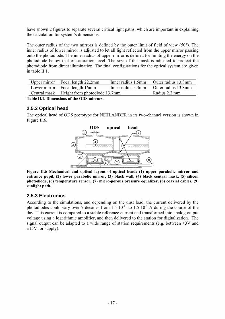
have shown 2 figures to separate several critical light paths, which are important in explaining the calculation for system’s dimensions. The outer radius of the two mirrors is defined by the outer limit of field of view (50°). The inner radius of lower mirror is adjusted to let all light reflected from the upper mirror passing onto the photodiode. The inner radius of upper mirror is defined for limiting the energy on the photodiode below that of saturation level. The size of the mask is adjusted to protect the photodiode from direct illumination. The final configurations for the optical system are given in table II.1.

Upper mirror Focal length 22.2mm Inner radius 1.5mm Outer radius 13.8mm Lower mirror Focal length 16mm Inner radius 5.3mm Outer radius 13.8mm Central mask Height from photodiode 13.7mm Radius 2.2 mm

Table II.1. Dimensions of the ODS mirrors.

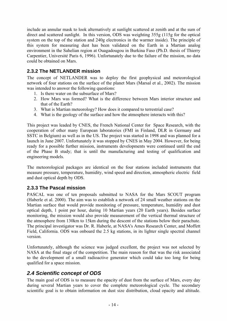
2.5.2 Optical head The optical head of ODS prototype for NETLANDER in its two-channel version is shown in Figure II.6.

Figure II.6 Mechanical and optical layout of optical head: (1) upper parabolic mirror and entrance pupil, (2) lower parabolic mirror, (3) black wall, (4) black central mask, (5) silicon photodiode, (6) temperature sensor, (7) micro-porous pressure equalizer, (8) coaxial cables, (9) sunlight path.

2.5.3 Electronics According to the simulations, and depending on the dust load, the current delivered by the photodiodes could vary over 7 decades from 1.5 10-11 to 1.5 10-4 A during the course of the day. This current is compared to a stable reference current and transformed into analog output voltage using a logarithmic amplifier, and then delivered to the station for digitalization. The signal output can be adapted to a wide range of station requirements (e.g. between ±3V and ±15V for supply).

- 18 -

Figure II.7 Picture of ODS optics (on the left) and electronics (on the right) prototypes.

2.6 Technical development and validation This section gives some overview of technical development and validation of ODS. The presentation then focuses on the work I realized in summer 2004 on validation and characterization of the field of view of ODS.

2.6.1 Overview of technical development of ODS The technical development of ODS, after the design in phase A, has been completed, following the scheme below:

1. Selection of photodiode detector 2. Manufacturing of the mirrors and optical head 3. Manufacturing, in parallel, of the electronics prototypes 4. Technical validation of electronic prototypes 5. Validation of optical field of view before assemblage 6. Assemblage of optical head by spatial glue 7. Re-validation of field of view after assemblage

After passing all stages above, the instrument will be ready for eventual vacuum, thermal and mechanical shock testing, if the mission was continued, and operation campaigns on terrestrial conditions. I have performed the validation of optical field of view before and after mechanical assemblage. These are presented in the next subsection.

2.6.2 ODS field of view characterization One of the most important quality to be controlled for the optical system of ODS is its field of view. Not only the field must be verified against theoretical design, it must also be measured to high precision as the accuracy of data retrieval procedure, presented in following chapters, depends on these characteristics.

- 19 -

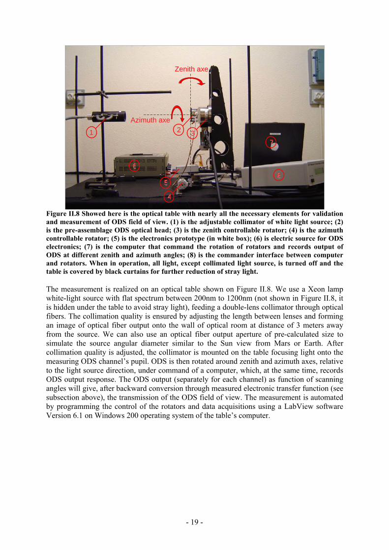
Figure II.8 Showed here is the optical table with nearly all the necessary elements for validation and measurement of ODS field of view. (1) is the adjustable collimator of white light source; (2) is the pre-assemblage ODS optical head; (3) is the zenith controllable rotator; (4) is the azimuth controllable rotator; (5) is the electronics prototype (in white box); (6) is electric source for ODS electronics; (7) is the computer that command the rotation of rotators and records output of ODS at different zenith and azimuth angles; (8) is the commander interface between computer and rotators. When in operation, all light, except collimated light source, is turned off and the table is covered by black curtains for further reduction of stray light. The measurement is realized on an optical table shown on Figure II.8. We use a Xeon lamp white-light source with flat spectrum between 200nm to 1200nm (not shown in Figure II.8, it is hidden under the table to avoid stray light), feeding a double-lens collimator through optical fibers. The collimation quality is ensured by adjusting the length between lenses and forming an image of optical fiber output onto the wall of optical room at distance of 3 meters away from the source. We can also use an optical fiber output aperture of pre-calculated size to simulate the source angular diameter similar to the Sun view from Mars or Earth. After collimation quality is adjusted, the collimator is mounted on the table focusing light onto the measuring ODS channel’s pupil. ODS is then rotated around zenith and azimuth axes, relative to the light source direction, under command of a computer, which, at the same time, records ODS output response. The ODS output (separately for each channel) as function of scanning angles will give, after backward conversion through measured electronic transfer function (see subsection above), the transmission of the ODS field of view. The measurement is automated by programming the control of the rotators and data acquisitions using a LabView software Version 6.1 on Windows 200 operating system of the table’s computer.

AAzziimmuutthh aaxxee

ZZeenniitthh aaxxee

11 22

77

8866

44

33

55

- 20 -

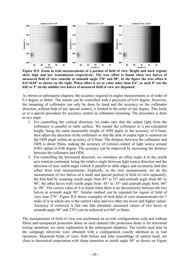
Figure II.9. Zoom in trial measurements of a portion of field of view. Bright and dark regions show high and low transmission respectively. The true offset is found when two halves of measured field of view coincide at azimuth angle 270° and 90°. In the figure the true offset is 0.6°±0.02° as shown on the right. When offset is set to value other than 0.6°, as such 0° (on the left) or 2° (in the middle) two halves of measured field of view are disjoined. As shown in subsequent chapters, the accuracy required in angles measurements is of order of 0.1 degree or better. The rotator can be controlled with a precision of 0.01 degree. However, the mounting of collimator can only be done by hand and the accuracy on the collimator direction, without help of any special control, is limited to the order of one degree. This leads us to a special procedure for accuracy control in collimator mounting. The procedure is done in two steps:

1. For controlling the vertical direction, we make sure that the output light from the collimator is parallel to table surface. We mount the collimator to a pre-calculated height, being the same measurable height of ODS pupil, to the accuracy of 0.5mm, then adjust the direction of the collimator so that the disk of output light is centered on the ODS pupil within an accuracy of 0.5mm. The distance between the collimator and ODS is about 50cm, making the accuracy of vertical control of light source around 0.001 radian or 0.06 degree. The accuracy can be improved by increasing the distance between the collimator and ODS.

2. For controlling the horizontal direction, we introduce an offset angle ∆ in the zenith axis rotation command, being the relative angle between light source direction and the direction of zero zenith angle (which is parallel to table edge), and accurately find this offset from trial measurements. Explicitly, in the trial measurement, we do the measurement of two halves of a small and special portion of field of view separately, the first half by scanning zenith angle from 45° to 55° and azimuth angle from 80° to 90°, the other haves with zenith angle from -45° to -55° and azimuth angle from -80° to -90°. The correct value of ∆ is found when there is no discontinuity between the two halves at azimuth angle 90°. Similar method can be repeated for region of field of view near 270°. Figure II.9 shows examples of trial field of view measurements for 3 trials of ∆ in which one is the correct value and two other are lower and higher values. Accuracy of retrieved ∆ (the one that minimize measured values of two haves at azimuth angle 90° and 270°) can be achieved at 0.04° or better.

The measurement of field of view was performed on several configurations with and without filters and transparent protection dome on each channel (the protection dome is for terrestrial testing operation; see more explanation in the subsequent chapters). The results used later in the campaign retrievals were obtained with a configuration exactly identical as in real operation. Measured fields of view, both before and after assemblage of optical head, are close to theoretical expectation with sharp transition at zenith angle 50° as shown on Figure

- 21 -

II.10. Figure II.11 gives more details on cross-section of the field of view for the blue channel of prototype 1, at several constant zenith and azimuth angles. We observe in the masked region at center of the field of view that there are still 4 small spots where the instrument response is significantly above zero. This can be seen on Figure II.11 by the curve corresponding to φ=60°. The explanation for this unexpected response is that the central masked was designed with a circular shape, which is intended to cover the circular sensible surface of the photodiode. In reality, the photodiode installed in the prototype has square shape and the four corners of this surface are not totally masked. Direct sunlight at some small inclination can partially arrive at these corners creating the observed features. In the future versions of ODS, we can modify the central mask for a square shape. Currently, the field of view has been accurately measured for use in the retrievals.

Figure II.10 Field of view of the red channel of the ODS prototype # 1 measured on the optical bench. White regions correspond to 100% transmission and black to 0%. Most light is collected between 25° and 50°. Shadowed sectors are due to the central mask supports.

Figure II.11. Cross-section of transmission field of view of blue channel of the ODS prototype 1 in the filters and protection dome configuration of terrestrial operation campaign, normalized so that maximum value of this field is set to 1. On the left are cross-sections corresponding to constant azimuth angles φ and on the right, cross-sections with constant zenith angles θ.

- 22 -

2.7 Conclusion The better understanding of the meteorology of the Martian atmosphere requires the measurement of temporal and geographical variability of atmospheric dust and water ice cloud. A convenient option for that might be a network of small stations carrying an Optical Depth Sensor, ODS, able to measure the right parameters over several seasonal cycles. We have shown that the design of ODS satisfies those scientific objectives as well as the strong technical constraints of a lightweight, small, long lifetime station deposited on the surface of the planet. A prototype has been built which measured optical characteristics have been shown to meet with the requirements of the NETLANDER mission. The following chapter will present the theoretical tools needed for simulating the anticipated signal and preparing the cloud opacity retrieval procedure.

- 23 -

Chapter 3

Models of radiative transfer in spherical atmosphere

3.1 Introduction In this chapter, we describe the development of a Monte-Carlo model and a Spherical Harmonics Discrete Ordinates Method (SHDOM) model, both in parallel-plane and spherical geometry. These two models will be used to simulate the responses of ODS for various setup of the instrument (e.g., filter colors, band-pass, field of views), as well as for various setup of the environmental conditions (e.g., the dust loading, the dust size distribution, the scattering geometry…). Actual measurements of ODS will be then compared to the simulations (forming then a database) in order to retrieve the main physical parameters of the dust layer and, in some cases, of the cloud layer. We have built a suite of models, both in plane-parallel and spherical geometry, and with both the Monte-Carlo and the SHDOM approaches. The purpose is to use the most adapted model for each case. Indeed, good simulations of daytime measurements (SZA smaller than 75°) can be achieved with a simple and fast parallel-plane model. But, on the other hand, simulations of ODS signal at sunrise and sunset (sun near or below horizon) require a model in spherical geometry, especially when clouds are observed. The Monte-Carlo method is accurate and robust, but slow. The SHDOM code is much faster. However, its accuracy must be controlled by comparisons to Monte-Carlo simulations, especially for the spherical geometry. In the following, the Monte-Carlo model will be used to build a database for a reference set of parameters of atmospheric properties and the SHDOM model will be used to expand the database of simulation into higher resolutions. In this chapter, we start with an introduction to the radiative transfer equations in planetary atmospheres. Then, we explain the two methods used to solve the radiative transfer equations: the Monte-Carlo method and SHDOM method. For each case, we explain first the main principle, and then we follow with detailed technical descriptions. Finally, we present different validation tests of the models with known analytic solutions. We finally show how the SHDOM compares with the Monte-Carlo model for selected cases.

3.2 Radiative transfer equations The main mathematical problem that must be solved now is to find the intensity of the sky, as seen from the ground, for various atmospheric models. To do so, we need to solve the radiative transfer equations. These equations describe how absorption and scattering processes affect the light coming from the Sun before arriving at the ODS photodiode. In this section, we briefly introduce the radiative transfer equations in the visible and near-infrared, and we present the main principles for the two numerical methods used to solve these equations. In the visible range, where thermal emissions and inelastic scattering (change in photon wavelength during scattering) can be ignored, the most significant processes of the radiative transfer are absorption and scattering. Consider a pencil of radiation traversing a medium. When the radiation crosses a slab of geometrical thickness dx, its intensity will be decreased by both absorption and scattering following the Beer-Lambert law:

- 24 -

dI = - βe I dx (III.1) Here, I is the intensity of the radiative field, βe is the extinction coefficient, being the sum of absorption and scattering coefficients. At the same time, the intensity is enhanced by the scattered light from all the directions into the traveling direction:

dI = + βe J dx (III.2) Here, J is the integration of scattered light from all direction into traveling direction of the pencil:

2 1

0 1

( , ) ( ', ') ( , , ', ') ' '4

J I P d dπωµ ϕ µ ϕ µ ϕ µ ϕ µ ϕ

π −

= ∫ ∫ (III.3)

Here P is the scattering phase function; ω is the single scattering albedo. The resulting equation of radiative transfer is:

dI = (–I + J) βe dx = (–I + J) dτ (III.4) Here τ is the extinction optical length (dτ = βe dx). We can integrate the equation into the integral form:

'),,'(),,0(),,(0

' τϕµτϕµϕµττ

ττ dJeeII ∫ −− += (III.5)

Here, the integration is done along the light-traveling path; I(τ) and I(0) are intensity at the beginning and the end of the path. Equation (III.3) and (III.5) are to be solved to find the intensity field inside the atmosphere. Generally, these coupled equations are difficult to solve analytically. The common approaches to the problem are numerical methods, including Monte-Carlo and Spherical Discrete Harmonics methods, which main principles are presented below.

3.3 Description of the Monte-Carlo model In this section, we describe the details of the Monte-Carlo model in parallel-plane and then in spherical geometry. Monte-Carlo models are robust and accurate, as shown later by validation tests. They will be used to compute the intensity field in several atmospheric cases, to provide reference results for the faster but less accurate SHDOM.

3.3.1 The principle of the Monte-Carlo approach Monte-Carlo is the name given to any method which solves a problem by using random numbers. The Monte-Carlo method is generally useful for obtaining numerical solutions of problems which are too complicated for an analytical resolution. It was suggested by Stanslaw Ulam, who in 1946 became the first mathematician to use this approach with a name (Metropolis and Ulam 1949; Hoffman 1998, p. 239). Nicolas Metropolis (Metropolis 1987) also contributed significantly to the development of the method. The most common application of the Monte Carlo method concerns the integration of complex integrals or high dimensions integrals. This method is also well adapted to problems which can be studied with a stochastic point of view, as for instance, the radiative transfer problem. In this case, the principle is to follow the fate of a large amount of particles (here photons) submitted to some physical laws, and to record a set of parameters (here, energy and propagation direction) along their motion for building a complete field. According to the theory of quantum physics, light (or generally electromagnetic wave) has a dual particle-wave nature. The propagation of the light in a medium can be considered as the motions of the wave trains, but also like "billiard balls", named photons, at the speed of the

- 25 -

light in the medium. The energy of a photon is hc/λ, where h is Planck constant, c is the speed of light, and λ is the wavelength. The quantum motions of photons are random, obeying to probabilistic laws. The processes of absorption and scattering in the atmosphere can thus be considered as stochastic processes. The phase function can be interpreted as a function of probability for the redistribution of the photons in various directions. Mathematically, the integrations of equations (III.3) and (III.5) can be performed numerically by a stochastic method ("Monte-Carlo integration"). In the weighted-Monte-Carlo integration method:

∑∫∫=

∞→==

N

i

i

NVV N

xfLimdGxfdxxgxf

1

)()()()( (III.6)

Where dG=gdx and g(x) is properly normalized: 1)( =∫

V

dxxg (III.7)

xi are randomly chosen within the integration region V obeying the distribution law g(x). Applying the above method to (III.3), we obtain:

2 1

10 1

( , )( , ) ( , , ', ') ' '4

Ni i

N i

IJ P d d LimN

π µ ϕωµ ϕ µ ϕ µ ϕ µ ϕπ →∞

=−

= × ∑∫ ∫ (III.8)

Here directions (µi,φi) randomly obey the distribution law of P(µ,φ). The same method make (III.5) becomes:

1

( )( ) (0)N

i

N i

JI I e LimN

τ ττ τ−

→∞=

= + ∑ (III.9)

Here τi are random obeying distribution law of e-τ. The Monte-Carlo radiative transfer simulation randomly launches packets of photons from a source and then follows each packet along their paths. The photons obey the stochastic law of absorption and scattering, until they escape from the atmosphere or until their intensity becomes negligible. By assigning the intensity as a property to the virtual packets of photon, the simulation of absorption is simply accounted by an exponential reduction of intensity along the random walk path. Random optical paths are generated according to Beer’s law, based on the scattering coefficient. At the end of the paths, new directions are chosen. The scattering angles are selected randomly from a distribution function which is proportional to the phase-function. With this method, we are able to know the state of the photons at each stage along their walking path and to deduce radiative quantities measured through photons collection by some virtual detector. The Monte-Carlo method is recognized to be the most accurate method for simulating absorption and scattering processes in the atmosphere. The only drawback is its time consumption but, as noted by Evans (1998), it should not be much slower than other methods as long as a moderated number of radiative quantities are desired.

3.3.2 Monte-Carlo model in a parallel-plane atmosphere The Monte-Carlo model for a parallel-plane atmosphere in use here is adapted from a model used by François Forget in Laboratoire de Météorologie Dynamique, C.N.R.S, France. The Figure III.1 shows a description of the physical processes for a packet of photons, in the case of a horizontally homogeneous parallel plane atmosphere.

- 26 -

After the launch, the packet enters in a loop of several processes which ends under specific conditions. It should be noted that we can simulate the collection of photons by a virtual detector at any stage of the loop. For example, to simulate the measurement of a ODS which is located on the surface of the planet, with a conical field of view of aperture (cosine of half angle) µODS, we collect all photons coming down to the surface, right before the stage "Reflection", if µ < -|µODS|.

Figure III.1 Diagram of multiple scattering random walk loop for a packet of photons in the Monte-Carlo radiative transfer simulation for parallel plane atmospheres. In this figure, I is the intensity of the radiative field, τs and τa are the optical thicknesses in term of scattering and absorption respectively, τs⊥ and τa⊥ are vertical projections of these optical thicknesses, µ and φ are the directions (cosine of zenith angle and azimuth angle) of motion of the packet, ∆µ and ∆φ are the scattering angles (cosine of zenith angle and azimuth angle), τ0 is the total scattering optical thickness of the atmosphere, µ0 and φ0 are the directions (cosine of zenith angle and azimuth angle) of the collimated source (Sun). We assume a Lambertian reflection at the surface, but other types of reflection laws are possible. For a horizontally homogeneous parallel-plane atmosphere, the vertical geometrical location can be replaced by the location in term of optical depth. This greatly accelerates the simulation because no conversion from geometric path to optical path (by integrating

- 27 -

extinction coefficient along geometrical path) is necessary. This simplification no longer holds in the case of spherical geometry, as shown in the next section.

3.3.3 Detailed description of the Monte-Carlo in spherical geometry Here, we present the details of the Monte-Carlo model for spherical atmospheres. We first display the input parameters of the model, which concerns the discretization set up and the physical properties of the planet and the atmosphere. We then describe the way the physical processes are linked together to produce the loop in which photons travel. We then show the output of the model.

Input parameters The first input to the Monte-Carlo code is the model of planetary atmosphere under interest. A spherically homogeneous atmosphere is specified by 3 parameters: scattering coefficients s(r), absorption coefficients a(r), and phase-functions P(θ, r) where r is the distance to the centre of the planet and θ is the scattering angle. Numerically, these functions are given at N discrete levels of r from r1 = R, planet solid body radius, to rN = R+T; T is geometrical thickness of the atmosphere. The phase-function is given, at each level, as 181 values between θ = 0° to θ = 180°. Intermediate values of the parameters are log-interpolated between the N discrete radius and 181 scattering angles. Extension to horizontally inhomogeneous atmosphere is possible by creating cells in the horizontal dimension. This extension is found to be of limited interest to planetary application since it complicates the calculation. It will not be mentioned further. The second input is the reflectivity of the planet surface. General reflection can be specified by a bi-directional distribution function. However, we rather assume a Lambertian reflection with only one parameter; the surface albedo as. The last inputs are the parameters which control the number of photons launched, the intensity threshold below which photons disappear, the way photons are initiated from the source (plane wave for the Sun, point source at center or any other distribution) and the way photons are collected.

Location and orientation in a spherical atmosphere In most planetary problems, the photon source is the Sun. We model it as a point source at infinity, generating a plane wave on the planet. We could as well include the realistic angular size of the Sun if needed; however as the size of Sun is small, this will make little change in the simulation. Figure III.2 shows the three axes of the coordinate system of calculation (Global Coordinate): the z axis is pointed toward the Sun, the x and y axes are perpendicular to z axis and to each other. The origin of the coordinate system is at the centre of the planet. A photon has the following associated coordinates (Figure III.2) and properties: position (3 numbers, P1 = cos(Θ), P2 = Φ, P3 = r), direction of motion (2 numbers: D1 = cos(Θd), D2 = Φd,) and intensity I. In calculations presented later, the direction of propagation of a photon is sometimes referred in the local coordinate system (subscript “l”): Dl1 = cos(Θld), Dl2 = Φld (Figure III.2). All processes are monochromatic, although an extension of the model to consider processes which change the photon’s wavelength (e.g. Doppler effect or fluorescence) is possible. Photons from the Sun will have an initial incident flux normalized to 1. Their initial direction is opposite to z (D1 = -1, D2 = arbitrary). Their initial position will be on the top layer of the atmosphere (P3 = R+T) and P1 and P2 are chosen in such a way that photons are distributed randomly over the cross-section of the atmosphere in direction z (P1

2 is random uniform within [0, 1], P2 random uniform within [0, 2π]).

- 28 -

Figure III.2 Global coordinate for referencing photon position and direction in the Monte-Carlo simulation for spherical atmosphere. Θ, Φ and Θd, Φd are respectively planeto-centric position and direction of the photon. The Sun is at Θ = Θd = 0. The direction d can also be referenced by a local coordinate system, Θld and Φld, where Θldis the local normal direction and Φld = 0° is taken in the anti-solar direction. Entering the atmosphere, the photons follow a loop of several physical processes (scattering, absorption, propagation, reflection,…). Each iteration begins with the choice for a free path in term of scattering optical depth, ∆τs, according to scattering law, P(∆τs) = exp(-∆τs).

Explicitly, ∆τs = F-1(x) with x uniform random in [0, 1] and ∫ ∆∆=x

ss dPxF0

)()( ττ . Here F(x)

is called the generating function of the probability distribution P(∆τs) (Papoulis 1984). So log( )s xτ∆ = − with x uniform random in [0, 1]. Note τs is the scattering optical depth along

traveling path defined by:

0

( ) ( ') 'l

s l s l dlτ = ∫ (III.10)

s(l) is the scattering coefficient. When photon trajectory l expands over several concentric cells, optical length is summed from integration within each cells ∆li:

10

( ) ( ') ' ( ') 'i

l n

s ii l

l s l dl s l dlτ= ∆

= = ∑∫ ∫ (III.11)

Here si(l) is the interpolated scattering coefficient in cell i and there are n cells. Geometric free path l, hence new position of photon at the end of free path, is numerically found (by a modified Newton method) by solving the equation τs(l) = ∆τs (with τs(l) given by (III.11) and ∆τs is the chosen free scattering optical path). Appendix 4 gives an analytical formulation for this equation when the scattering coefficient is linearly interpolated between layers. At its new location, photons experience a scattering where the azimuthal scattering angle ∆φ is randomly chosen in the range [0, 2π] and the zenithal scattering angle ∆θ is randomly chosen from accordingly to the phase-function P(∆θ). Explicitly, ∆θ = F-1(x) with x uniform random in [0, 1] and F(x) is the generating function of the phase function P(θ),

- 29 -

∫=x

dPxF0

)()( θθ . Before going on the iteration, the intensity is reduced by the absorption law

Iend = Istart exp(-τa(l)). Absorption optical depth τa is defined similarly to scattering optical depth (equation (III.10) replacing s by a). Whenever the photons altitude gets below zero, the direction is changed at the surface by a lambertian reflection (Dl1 uniform random in [0,1], Dl2 = uniform random in [0, 2π] where Dl1 and Dl2 are direction relative to local surface) and the photons continue the remaining part of the free-path, ∆τs, above surface. Reflection on surface yields an additional absorption given by Inew = as Iold. The end of the photons random walk happens whenever the intensity of photon gets below a minimum value (I < Imin with Imin is generally set between 10-3 and 10-6) or when the photons escape from the atmosphere (P3 > R+T).

l Figure III.3 Diagram of the multiple scattering random walk loop for a packet of photon in the Monte-Carlo radiative transfer simulation for the spherical atmosphere. See section text for the

- 30 -

description of parameters in the figure (I, P3, D1, D2 …). The surface reflection is of the type Lambertian. Figure III.3 summarizes the multiple scattering loop of a packet of photons in the Monte-Carlo model for a spherical atmosphere. It should be noted that the actual calculation contains more detail than presented in the diagram; in particular the determination of the positions P1 and P2 in parallel with calculation of P3 which are necessary for conversion between global directions D1, D2 and local directions Dl1, Dl2 (Appendix 1). As for the parallel-plane model, we can also add a virtual collector of photons at any place in the diagram. The production of the final outputs is explained in more details in the following section.

Output of the code The Monte-Carlo code is flexible concerning the setup of the detector. For remote sensing from outside of the atmosphere, all photons escaping from the atmosphere may be stored in positional bins at the top atmospheric layer and directional bins relative to local the normal direction. For observation from the planet surface, the incoming photon may be stored in positional bins on the surface and directional bins relative to the local surface. Thank to the symmetry of the problem, the positional bin can simply be parallel strips at different latitudes P1 in Global Coordinate. The intensity, at a given bin (P1 ± ∆P1, Dl1 ± ∆Dl1, Dl2 ± ∆Dl2) and at an altitude z, is found from photon flux F (sum of intensity of all incoming photon) by:

2

20 1 1 1 2

( ) 12 l l l

F R zIF R P D D D

+=

∆ ∆ ∆ (III.12)

Here, as mentioned before, Dl1 and Dl2 are zenithal and azimuthal angles relative to local surface. The intensity field can be interpolated from values in the bins. The process of collecting the photons by a virtual detector is Poissonian. Hence the signal-to-noise ratio is proportional to the square root of total number of photons collected. This implies that the Monte-Carlo code will converge faster if the fields of view (∆Dl1 and ∆Dl2) or the size (∆P1) of detector are large. The Monte-Carlo simulation can be accelerated if we use quasi-random number in generating free scattering path and scattering angle (O’Brien 1992).

3.4 SHDOM in spherical atmosphere Here we describe the details of the Spherical Harmonic Discrete Ordinate method (SHDOM) model for a spherical atmosphere. We first describe the principle. Then, we consider a problem, which arises when we try to expand the forward phase functions into Legendre polynomials, and we introduce an adapted scheme. In a third part, we explain how the parallel-plane geometry and the spherical geometry are treated in the SHDOM model. Finally – as for the Monte-Carlo model – we describe the inputs of the model, the stages of the iteration loop and finally, how are defined the outputs.

3.4.1 Principle of the SHDOM approach Another way to solve the radiative transfer equations (III.3) and (III.5) is by the discrete ordinate method (Gerstl and Zardecki 1985) in which one tries to linearize the system through the finite-element approach. We approximate the integrations in (III.3) and (III.5) by summations over chosen discrete directions and locations in the atmosphere. This reduces the coupled equations to a recurrent relation where the quantity to seek for is the radiative field itself, in the fixed-point relation:

I = f(I) (III.13)

- 31 -

Or, through a simple matrix operation, as show later:

I = M×I + M0 (III.14) Upon this relation, a Picard iteration (a fixed-point iteration for finding a series of functions that converges to a solution of a differential equation, Kuo et al. 1996) or Λ iteration (a type of Picard iteration adapted to radiative transfer equations, Stenholm et al.1991, Evans 1998) may be used to find the convergence field, starting with a simple initial field (single scattering solution or just zero field) as a first set of parameter for I. Published discrete ordinate schemes differ from each others in the choice of the discrete model grid, discrete angles and discrete basis of functions for series expansion of radiative transfer properties. In particular, for the choice of discrete directions, many discrete ordinate codes use the Gaussian quadrature approximation for evaluation of (III.3) or of any other quantity which requires an angular integration:

4

( )f d d dπ∫ =

2 1

0 1

( , )f d dπ

ϕ µ

µ ϕ µ ϕ= =−∫ ∫ =

( )

1 1

( , )N N i

ij i ji j

w fµ ϕ

µ ϕ= =∑ ∑ (III.15)

Here Nµ is the number of Gaussian quadratures for cosine zenith angle µi between [-1, 1]; Nφ is the number of discrete azimuth direction φj. Nφ may vary with zenith direction; wij are the integration weights (if φj are equally spaced then wij = 2πwi/Nφ where wi are Gaussian integration weights). Evans (1998) had successfully implemented a faster and more accurate approach for integration of the source function in (III.3), using an intermediate step of angular spherical harmonic expansion for radiance field. It is known that spherical harmonics form a complete orthogonal basis of functions over the sphere, then any intensity field at any given position in the atmosphere can be approximated by a truncated series as:

f(µ,φ) = 0

( ) ( )sN l

mlm l

l m l

f u m Pϕ µ= =−∑∑ (III.16)

Here u(mφ) is sin(mφ) for m<0 and cos(mφ) otherwise; The ( )mlP µ are the associated

Legendre polynomials of degree l and rank m, and Ns is the truncation order. Normally, Ns is the same order as Nµ and Nφ. The discrete ordinate source function J is found from the discrete ordinate intensity I through three steps. The first step is the conversion of the discrete ordinate field I into spherical harmonic expansion coefficients Ilm, which is the projection of the intensity field onto orthogonal basis of spherical harmonics:

Ilm = ( )

1 1

( , ) ( ) ( )N N i

lij i j j m i

i j

w I u m Pµ ϕ

µ ϕ ϕ µ= =∑ ∑ (III.17)

Then we integrate (III.3) in the space of spherical harmonics by a simple linear operation (which is a consequent of Spherical Harmonic Addition Theorem, §12.8 in Arfken 1995):

Jlm = 2 1

l

lχ+

Ilm (III.18)

Here χl is the coefficient in the truncated Legendre series approximation of the phase-function P(θ)

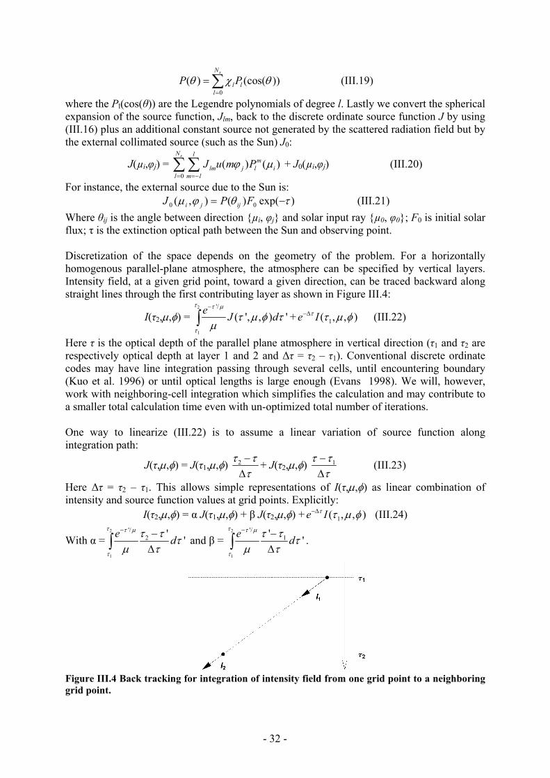
- 32 -

0

( ) (cos( ))sN

l ll

P Pθ χ θ=

= ∑ (III.19)

where the Pl(cos(θ)) are the Legendre polynomials of degree l. Lastly we convert the spherical expansion of the source function, Jlm, back to the discrete ordinate source function J by using (III.16) plus an additional constant source not generated by the scattered radiation field but by the external collimated source (such as the Sun) J0:

J(µi,φj) = 0

( ) ( )sN l

mlm j l i

l m l

J u m Pϕ µ= =−∑∑ + J0(µi,φj) (III.20)

For instance, the external source due to the Sun is: )exp()(),( 00 τθϕµ −= FPJ ijji (III.21)

Where θij is the angle between direction {µi, φj} and solar input ray {µ0, φ0}; F0 is initial solar flux; τ is the extinction optical path between the Sun and observing point. Discretization of the space depends on the geometry of the problem. For a horizontally homogenous parallel-plane atmosphere, the atmosphere can be specified by vertical layers. Intensity field, at a given grid point, toward a given direction, can be traced backward along straight lines through the first contributing layer as shown in Figure III.4:

I(τ2,µ,φ) = 2

1

'/

( ', , ) 'e J dτ τ µ

τ

τ µ φ τµ

−

∫ + 1( , , )e Iτ τ µ φ−∆ (III.22)

Here τ is the optical depth of the parallel plane atmosphere in vertical direction (τ1 and τ2 are respectively optical depth at layer 1 and 2 and ∆τ = τ2 – τ1). Conventional discrete ordinate codes may have line integration passing through several cells, until encountering boundary (Kuo et al. 1996) or until optical lengths is large enough (Evans 1998). We will, however, work with neighboring-cell integration which simplifies the calculation and may contribute to a smaller total calculation time even with un-optimized total number of iterations. One way to linearize (III.22) is to assume a linear variation of source function along integration path:

J(τ,µ,φ) = J(τ1,µ,φ) 2τ ττ−∆

+ J(τ2,µ,φ) 1τ ττ−∆

(III.23)

Here ∆τ = τ2 – τ1. This allows simple representations of I(τ,µ,φ) as linear combination of intensity and source function values at grid points. Explicitly:

I(τ2,µ,φ) = α J(τ1,µ,φ) + β J(τ2,µ,φ) + 1( , , )e Iτ τ µ φ−∆ (III.24)

With α =2

1

'/2 ' 'e d

τ τ µ

τ

τ τ τµ τ

− −∆∫ and β =

2

1

'/1' 'e d

τ τ µ

τ

τ τ τµ τ

− −∆∫ .

Figure III.4 Back tracking for integration of intensity field from one grid point to a neighboring grid point.

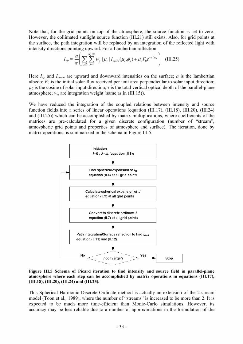
- 33 -

Note that, for the grid points on top of the atmosphere, the source function is set to zero. However, the collimated sunlight source function (III.21) still exists. Also, for grid points at the surface, the path integration will be replaced by an integration of the reflected light with intensity directions pointing upward. For a Lambertian reflection:

Iup = 0

( )/

0 00 1

| | ( , )i

N i

ij i down i jj

a w I F eφ

τ µ

µ

µ µ φ µπ

−

≤ =

⎛ ⎞+⎜ ⎟

⎝ ⎠∑ ∑ (III.25)

Here Iup and Idown are upward and downward intensities on the surface; a is the lambertian albedo; F0 is the initial solar flux received per unit area perpendicular to solar input direction; µ0 is the cosine of solar input direction; τ is the total vertical optical depth of the parallel-plane atmosphere; wij are integration weight (same as in (III.15)). We have reduced the integration of the coupled relations between intensity and source function fields into a series of linear operations (equation (III.17), (III.18), (III.20), (III.24) and (III.25)) which can be accomplished by matrix multiplications, where coefficients of the matrices are pre-calculated for a given discrete configuration (number of “stream”, atmospheric grid points and properties of atmosphere and surface). The iteration, done by matrix operations, is summarized in the schema in Figure III.5.

Figure III.5 Schema of Picard iteration to find intensity and source field in parallel-plane atmosphere where each step can be accomplished by matrix operations in equations (III.17), (III.18), (III.20), (III.24) and (III.25). This Spherical Harmonic Discrete Ordinate method is actually an extension of the 2-stream model (Toon et al., 1989), where the number of “streams” is increased to be more than 2. It is expected to be much more time-efficient than Monte-Carlo simulations. However, its accuracy may be less reliable due to a number of approximations in the formulation of the

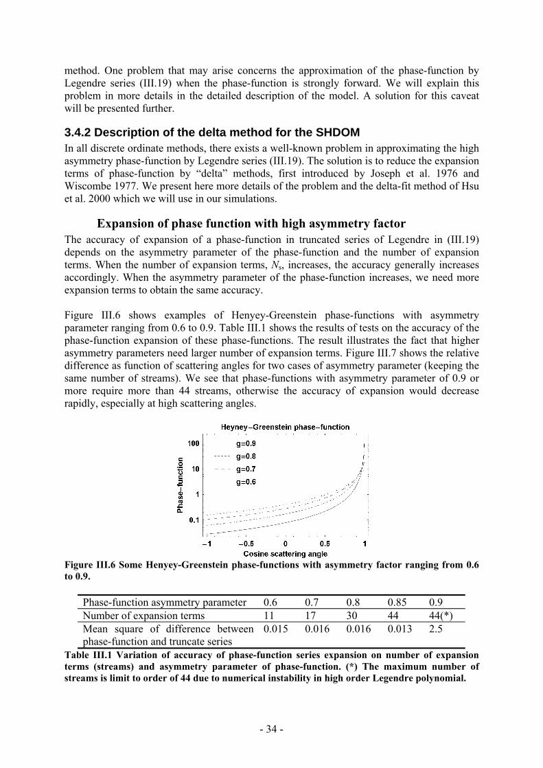
- 34 -

method. One problem that may arise concerns the approximation of the phase-function by Legendre series (III.19) when the phase-function is strongly forward. We will explain this problem in more details in the detailed description of the model. A solution for this caveat will be presented further.

3.4.2 Description of the delta method for the SHDOM In all discrete ordinate methods, there exists a well-known problem in approximating the high asymmetry phase-function by Legendre series (III.19). The solution is to reduce the expansion terms of phase-function by “delta” methods, first introduced by Joseph et al. 1976 and Wiscombe 1977. We present here more details of the problem and the delta-fit method of Hsu et al. 2000 which we will use in our simulations.

Expansion of phase function with high asymmetry factor The accuracy of expansion of a phase-function in truncated series of Legendre in (III.19) depends on the asymmetry parameter of the phase-function and the number of expansion terms. When the number of expansion terms, Ns, increases, the accuracy generally increases accordingly. When the asymmetry parameter of the phase-function increases, we need more expansion terms to obtain the same accuracy. Figure III.6 shows examples of Henyey-Greenstein phase-functions with asymmetry parameter ranging from 0.6 to 0.9. Table III.1 shows the results of tests on the accuracy of the phase-function expansion of these phase-functions. The result illustrates the fact that higher asymmetry parameters need larger number of expansion terms. Figure III.7 shows the relative difference as function of scattering angles for two cases of asymmetry parameter (keeping the same number of streams). We see that phase-functions with asymmetry parameter of 0.9 or more require more than 44 streams, otherwise the accuracy of expansion would decrease rapidly, especially at high scattering angles.

Figure III.6 Some Henyey-Greenstein phase-functions with asymmetry factor ranging from 0.6 to 0.9.

Phase-function asymmetry parameter 0.6 0.7 0.8 0.85 0.9 Number of expansion terms 11 17 30 44 44(*) Mean square of difference between phase-function and truncate series

0.015 0.016 0.016 0.013 2.5

Table III.1 Variation of accuracy of phase-function series expansion on number of expansion terms (streams) and asymmetry parameter of phase-function. (*) The maximum number of streams is limit to order of 44 due to numerical instability in high order Legendre polynomial.

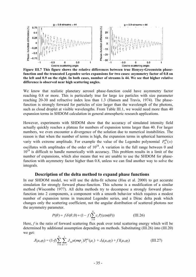
- 35 -

Figure III.7 This figure shows the relative differences between true Henyey-Greenstein phase-function and the truncated Legendre series expansions for two cases: asymmetry factor of 0.8 on the left and 0.9 on the right. In both cases, number of streams is 44. We see that higher relative difference is observed near high scattering angles. We know that realistic planetary aerosol phase-function could have asymmetry factor reaching 0.8 or more. This is particularly true for large ice particles with size parameter reaching 20-30 and refractive index less than 1.3 (Hansen and Travis, 1974). The phase-function is strongly forward for particles of size larger than the wavelength of the photons, such as cloud droplet at visible wavelengths. From Table III.1, we would need more than 40 expansion terms in SHDOM calculation in general atmospheric research applications. However, experiments with SHDOM show that the accuracy of simulated intensity field actually quickly reaches a plateau for numbers of expansion terms larger than 40. For larger numbers, we even encounter a divergence of the solution due to numerical instabilities. The reason is that when the number of terms is high, the expansion terms in spherical harmonics variy with extreme amplitude. For example the value of the Legendre polynomial 40

16 ( )P x oscillates with amplitudes of the order of 1024. A variation in the full range between 0 and 1024 is difficult to handle numerically with accuracy. This problem results in a limit of the number of expansions, which also means that we are unable to use the SHDOM for phase-function with asymmetry factor higher than 0.8, unless we can find another way to solve the integrals.

Description of the delta method to expand phase functions In our SHDOM model, we will use the delta-fit scheme (Hsu et al. 2000) to get accurate simulation for strongly forward phase-function. This scheme is a modification of a similar method (Wiscombe 1977). All delta methods try to decompose a strongly forward phase-function into 2 components, a component with a smooth behavior which requires a modest number of expansion terms in truncated Legendre series, and a Dirac delta peak which changes only the scattering coefficient, not the angular distribution of scattered photons nor the asymmetry parameter.

0

( ) ( ,0) (1 ) (cos( ))sN

l ll

P f f c Pθ δ θ θ=

= + − ∑ (III.26)

Here, f is the ratio of forward scattering flux peak over total scattering energy which will be determined by additional assumption depending on methods. Substituting (III.26) into (III.20) we get:

J(µi,φj) = (1-f)0

( ) ( )sN l

mlm j l i

l m l

J u m Pϕ µ= =−∑∑ + J0(µi,φj) + f I(µi,φj) (III.27)

- 36 -

The Dirac delta-like forward scattering peak would require an infinite number of expansion terms all having values equal to the integration of delta peak. If we could take the peak out of the integration for the source function, we would actually remove the infinite number of expansion terms. In this manner, we simulate scattering process only with the part of the phase-function which can be expanded. Delta-methods differ from each other in the calculation of forward peak ratio f and the determination of expansion terms. Wiscombe (1977) suggests, in the delta-M method, to find factor f and expansion terms cl in (III.26) from the integration of Legendre polynomial. To improve the accuracy as well as the computational speed by archiving a limited number of expansion terms, Hsu et al. 2000 replaced the usual coefficients in the Legendre polynomial expansions (which are the projection of the function on an orthogonal basis) by new coefficients computed from a weighted least-squares fitting procedure. The coefficients cl are found by minimizing the relative difference between the sum

0

(cos( ))sN

l ll

c P θ=∑ and the “chopped phase function”, that is, the phase-function without its

forward peak. To remove the forward peak, we simply set the “chopped phase function” constant for scattering angle smaller than a given small angle α which contains the forward peak. Given a fixed number of streams, N, and a fixed tolerance, ε, the delta-fit algorithm tries to repeatedly increase the forward peak removal angle, α, and fit the chopped phase-function to Legendre sum until least-square difference is inferior than ε. The resulting sum

0

(cos( ))sN

l ll

c P θ=∑ is the best fit of chopped phase-function, P’(θ). In this case, the coefficients cl

are different from the components of the phase function projected on the orthogonal basis. By normalization:

( )1 1

1 11

01

0

4 2 (cos( )) (cos( )) 2 ( ) '( ) (cos( ))

4 2 (cos( )) (cos( ))

4 4

sN

l ll

P d f P d

f c P d

f c

π π θ θ π δ θ θ θ

π π θ θ

π π

− −

=−

= = +

= +

= +

∫ ∫

∑∫ (III.28)

In (III.28) we have use the fact that1

01

( ) 1P dµ µ−

=∫ and 1

1

( ) 0lP dµ µ−

=∫ for l > 0. So we obtain:

f = 1- c0 (III.29) where c0 is the zero-order best fit coefficient. Here f can be considered as the fraction of “un-scattered” energy (highly forward scattered). So the actual scattered energy or the effective scattering coefficient is only c0 times the original ones.

seffective = s c0 (III.30)

After the effective scattering coefficient is found by (III.30), the effective phase function

0

(cos( ))sN

l ll

c P θ=∑ is normalized to

0 0

(cos( ))sN

ll

l

c Pc

θ=∑ in order to conserve the energy. In this way,

we consider scatterers that have an effective scattering efficiency smaller than their real efficiency, and with effective chopped phase functions normalized to 1. The difference between the actual scattering efficiency and the effective scattering efficiency corresponds to

- 37 -

photons which was previously contained in the forward peak, and are now assumed to continue without interaction. The SHDOM simulation will work with a forward-peak-removed phase-function represented by the normalized coefficients cl/c0 and effective scattering coefficient in (III.30).

3.4.3 SHDOM in spherical geometry In the case of SHDOM, dealing with the spherical geometry generates complications for several reasons: cell-to-cell relations of radiation and source function require additional relation between different solar angles, additional conversions between local discrete angles (for each solar zenith angle) and surface reflection is difficult to account with global direction discretization (same for all solar zenith angle). To avoid the complexity when accounting for the exact spherical geometry, we must make reasonable approximations. First, we can assume that, for most planetary atmospheres in the Solar System, the scattered radiation field in spherical atmosphere is nearly identical to that in parallel-plane atmosphere for solar zenith angle smaller than about 70° to 80°. On the other hand, the spherical effect is generally significant only for SZA between 0° and 100°. Then we can reduce to 20%-30% the amount of computation with a spherical geometry. Figure III.8 shows the comparison of optical depth in the sun direction as a function of the solar zenith angle in a parallel plane atmosphere and in a spherical atmosphere. The normal (vertical) optical depth and the planet radius are taken to 1 and 3400km (Martian radius) respectively. For solar zenith angle smaller than 75°, the relative difference remains smaller than 5%. This is equivalent to a 2% difference in intensity field (assumed to be in the order of the difference of exponential of optical depth).

Figure III.8 Comparison between optical lengths from Sun to ground in two geometries: spherical and parallel plane. Both optical depths are calculated with same representative model of Martian atmosphere: radius of planet in spherical geometry is 3400km, optical depth 1, vertical profile exponential with scale height 10km, single scattering albedo 0.5. On the left shows the two optical depths. On the right is the relative difference in %. We see that as solar zenith angle (SZA) increases, parallel geometry gives higher and higher optical depth than spherical case. Until SZA about 75°, the relative difference is still lower than 5%. Secondly, we assume that for solar zenith angles between 75° and 100°, the spherical radiation field can be approximated by a two-dimensional Cartesian frame, where the two dimensions are the vertical optical layer and the solar zenith angle (directional dimensions are always zenith and azimuth angular directions). Figure III.9 explains this idea. In spherical geometry, there is a global grazing solar input source which may be viewed at different local solar zenith angle on different part of the planet. Further, for solar zenith angles higher than 90°, the source is shadowed by the planet solid body at low altitude (Figure III.9, left). The right part of Figure III.9 is an “equivalent” two-dimensional parallel-plane atmosphere. The

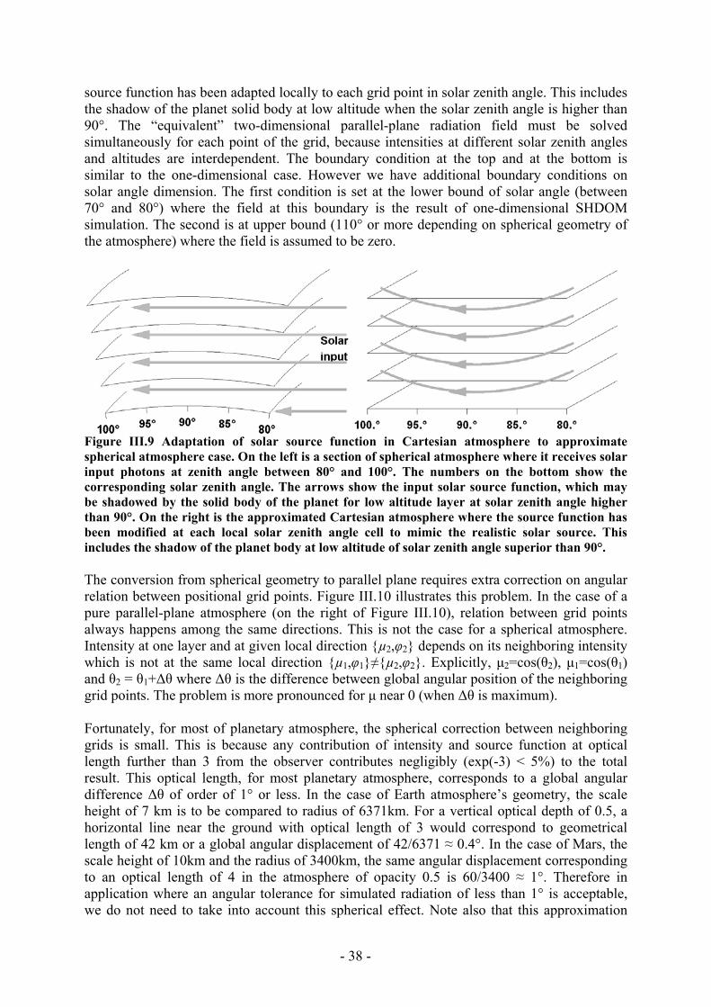
- 38 -

source function has been adapted locally to each grid point in solar zenith angle. This includes the shadow of the planet solid body at low altitude when the solar zenith angle is higher than 90°. The “equivalent” two-dimensional parallel-plane radiation field must be solved simultaneously for each point of the grid, because intensities at different solar zenith angles and altitudes are interdependent. The boundary condition at the top and at the bottom is similar to the one-dimensional case. However we have additional boundary conditions on solar angle dimension. The first condition is set at the lower bound of solar angle (between 70° and 80°) where the field at this boundary is the result of one-dimensional SHDOM simulation. The second is at upper bound (110° or more depending on spherical geometry of the atmosphere) where the field is assumed to be zero.

Figure III.9 Adaptation of solar source function in Cartesian atmosphere to approximate spherical atmosphere case. On the left is a section of spherical atmosphere where it receives solar input photons at zenith angle between 80° and 100°. The numbers on the bottom show the corresponding solar zenith angle. The arrows show the input solar source function, which may be shadowed by the solid body of the planet for low altitude layer at solar zenith angle higher than 90°. On the right is the approximated Cartesian atmosphere where the source function has been modified at each local solar zenith angle cell to mimic the realistic solar source. This includes the shadow of the planet body at low altitude of solar zenith angle superior than 90°. The conversion from spherical geometry to parallel plane requires extra correction on angular relation between positional grid points. Figure III.10 illustrates this problem. In the case of a pure parallel-plane atmosphere (on the right of Figure III.10), relation between grid points always happens among the same directions. This is not the case for a spherical atmosphere. Intensity at one layer and at given local direction {µ2,φ2} depends on its neighboring intensity which is not at the same local direction {µ1,φ1}≠{µ2,φ2}. Explicitly, µ2=cos(θ2), µ1=cos(θ1) and θ2 = θ1+∆θ where ∆θ is the difference between global angular position of the neighboring grid points. The problem is more pronounced for µ near 0 (when ∆θ is maximum). Fortunately, for most of planetary atmosphere, the spherical correction between neighboring grids is small. This is because any contribution of intensity and source function at optical length further than 3 from the observer contributes negligibly (exp(-3) < 5%) to the total result. This optical length, for most planetary atmosphere, corresponds to a global angular difference ∆θ of order of 1° or less. In the case of Earth atmosphere’s geometry, the scale height of 7 km is to be compared to radius of 6371km. For a vertical optical depth of 0.5, a horizontal line near the ground with optical length of 3 would correspond to geometrical length of 42 km or a global angular displacement of 42/6371 ≈ 0.4°. In the case of Mars, the scale height of 10km and the radius of 3400km, the same angular displacement corresponding to an optical length of 4 in the atmosphere of opacity 0.5 is 60/3400 ≈ 1°. Therefore in application where an angular tolerance for simulated radiation of less than 1° is acceptable, we do not need to take into account this spherical effect. Note also that this approximation

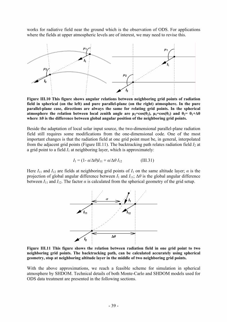
- 39 -

works for radiative field near the ground which is the observation of ODS. For applications where the fields at upper atmospheric levels are of interest, we may need to revise this.

Figure III.10 This figure shows angular relations between neighboring grid points of radiation field in spherical (on the left) and pure parallel-plane (on the right) atmosphere. In the pure parallel-plane case, directions are always the same for relating grid points. In the spherical atmosphere the relation between local zenith angle are µ2=cos(θ2), µ1=cos(θ1) and θ2= θ1+∆θ where ∆θ is the difference between global angular position of the neighboring grid points. Beside the adaptation of local solar input source, the two-dimensional parallel-plane radiation field still requires some modifications from the one-dimensional code. One of the most important changes is that the radiation field at one grid point must be, in general, interpolated from the adjacent grid points (Figure III.11). The backtracking path relates radiation field I2 at a grid point to a field I1 at neighboring layer, which is approximately:

I1 = (1- α/∆θ)I11 + α/∆θ I12 (III.31)

Here I11 and I12 are fields at neighboring grid points of I1 on the same altitude layer; α is the projection of global angular difference between I1 and I11; ∆θ is the global angular difference between I11 and I12. The factor α is calculated from the spherical geometry of the grid setup.

Figure III.11 This figure shows the relation between radiation field in one grid point to two neighboring grid points. The backtracking path, can be calculated accurately using spherical geometry, stop at neighboring altitude layer in the middle of two neighboring grid points. With the above approximations, we reach a feasible scheme for simulation in spherical atmosphere by SHDOM. Technical details of both Monte-Carlo and SHDOM models used for ODS data treatment are presented in the following sections.

- 40 -

3.4.4 Input to simulation The first input to the Spherical Harmonic Discrete Ordinate (SHDOM) code is the model of planetary atmosphere into consideration. A spherically homogeneous atmosphere is specified by 3 parameters: scattering coefficient s(r), absorption coefficient a(r), and phase-function P(θ, r) where r is the distance to planet center and θ is the scattering angle. Numerically, these functions are input at N discrete values of r from r1 = R, the planet solid body radius, to rN = R+T; T is the geometrical thickness of the atmosphere. The phase-function can be given, at each ri, as discrete value (for example, 181 values between θ = 0° to θ = 180°) or as accurate symbolic form in computer algebra system (such as Mathematica, Wolfram 1999) where the manipulation on phase-function can be done symbolically. The next input is the surface reflectivity. The current version of SHDOM code supports the most popular type of reflection in planetary research, Lambertian reflection with only parameter being albedo as. These inputs are similar to the case of the Monte-Carlo simulations. The final inputs are parameters controlling the accuracy and the calculation time of simulation. They are a number of expansion terms (or “streams”) in phase-function, resolution on discrete solar angle grid, and tolerance for convergence of solution of intensity field.

3.4.5 Details of simulation In the two-dimensional pseudo-spherical atmosphere, the simulation is done through the steps described in Figure III.12. There are three main blocks in the simulation scheme, the preparation block, the self-consistent matrix equation loop and the output conditioning block. Most of the complexity is concentrated in the preparation block. The purpose of this block is to prepare the iterative operations to be performed on the intensities and the source functions. The intensity field and the source functions can be represented under the form of matrices. The operators are also in the matrix forms: the surface reflection matrix R, the scattering matrix S, the absorption matrix A and the path integration matrix P. Here the matrix R operates on the sky scattered intensity field (especially the downward field at surface) and gives the reflected field (explicitly, the upward field at surface) following the Lambertian reflection law. Because R only acts on the scattered field, the correct reflected field must also include the reflected component of direct field at surface, I0 (III.25). The matrix S operates on the discrete ordinate scattered intensity field to give discrete ordinate source function. Again S does not act on the direct solar input intensity and the total source function must include the source function due to this component, J0 (S is the combination of operations in equations III.17, III.18 and III.20). The absorption matrix A and the path integration matrix P related intensity field at one grid point to respectively intensity and source function at neighboring grid points, through equation (III.24) and (III.31).

- 41 -

Figure III.12 Details of two-dimensional pseudo-spherical Spherical Harmonic Discrete Ordinate simulation. All the matrices can be prepared once for all at the beginning, after inputs to the code are checked for validity, and stored. The reflection matrix R depends only on the number of streams, which determines the discrete directions and the integration weights. The scattering matrix S can be found from pre-calculated discrete parameters and Legendre coefficients of phase-function after the delta-fit scheme. The delta-fit scheme also gives modified scattering and absorption coefficients which help building up optical lengths between layers along discrete direction. The calculation of the optical length matrix uses the exact spherical geometry, with the assumption that scattering and absorption coefficient vary linearly or log-linearly (the later is the preferable choice in later simulations) between the altitude grid-points. With the optical length matrix we can deduce both absorption matrix A, the solar input source J0 and reflected field I0. The accurate geometrical calculation also gives interpolation matrix (III.31) which when combined with optical depth matrix gives the path integration matrix P. In the iteration loop, we choose the Picard iteration scheme as shown in Figure III.12. New intensity, in each iteration loop, is found through conversion back and forth with source function. When the relative change in the field (∆I/I) smaller than some convergence tolerance ε, we get out of the solution loop to the final output conditioning. One could simplify the iteration in Figure III.12 into a form:

In+1 = C + M In (III.32) However, we found that the size of M and C would require large memory storage and actually much slower computation than decomposing the iteration into steps shown. At each steps, the

- 42 -

matrices are actually stored in very compact form internally in the computer memory, by taking advantages of their symmetries. For example, surface reflection matrix has only 1 dimension with length being the number of upward streams, because this matrix only applies to the surface layer and is the same for all position on the surface. The matrices multiplication are therefore not done straightly but by linear operations specifically adapted to the internal format of the matrices.

3.4.6 Output of the code The output is given as an interpolated radiance factor (I/F) as a function of the directions {µ, φ}, the altitude z and solar zenith angle θ. The interpolation may require regular rectangle array values of direction {µ, φ} instead of irregular pre-calculated discretization during the solution phase. Also it may require interpolation at pole of field (µ = -1 and 1) as these directions are not included in Gaussian discretization in zenith direction. The output interpolated function can be used later as any continuous function (such as in Mathematica environment, Wolfram 1999) in derivation of any related radiative properties. For instance, the flux received by an instrument like ODS, which probes the sky from ground, can be found by:

2

1

2

0

( ) ( , ,0, )f I d dµπ

µ

θ µ ϕ θ µ ϕ= ∫ ∫ (III.33)

Here µ1 and µ2 are cosine of the boundary zenithal angles of ODS field of view.

3.5 Validations and comparisons Before using the Monte-Carlo and the SHDOM models, especially in the spherical geometry, we must carefully validate them against exact solutions found in the literature. In this section, we focus on two aspects. First we test the validity of the computation of opacities in the parallel-plane and spherical geometry. To do so, we compare our models with simple single scattering models, for which analytical solutions can be found easily. Secondly, we test the multiple scattering processes. We then compare our models with well known solutions of scattering by a semi infinite parallel plane atmosphere published by Chandrasekhar (1960). For the Monte-Carlo model, we are able to further examine the model’s robustness in both aspects, multiple scattering and in spherical geometry, by using a point source at the origin of an infinite spherical atmosphere. The result of this simulation will be compared with some exact solutions of statistical mechanics and also a solution of Chandrasekhar (1960). Once these tests are successful, we can assume that the Monte-Carlo model is fully validated. We then compare simulations between the Monte-Carlo and the SHDOM models for 4 cases of realistic atmospheres. Our purpose here is to estimate the accuracy of the SHDOM model, in multiple scattering spherical atmospheres, especially at large solar zenithal angles that ODS is supposed to observe.

3.5.1 Comparison with single scattering solutions A unique capability of the Monte Carlo simulation is that it can easily separate the result for the different orders of scattering. In particular, the code can simulate the single scattering by adding a control to stop the random walk of photon when the number of scattering exceeds 1. Meanwhile, the SHDOM code can also simulate the single scattering solution by limiting the iteration to one loop, where the path integration of source function is extended to the

- 43 -

boundaries of the atmosphere instead of nearest neighbor grid points. These small modifications offer a convenient way to examine the simulations of the two models against single scattering cases for which analytical solutions are known. The successful tests will ensure the validity of the optical paths in the parallel-plane and the spherical geometry models.

Parallel-plane geometry For parallel-plane geometry, we concentrate on the observation of sky scattered intensity from the surface when the sun is at zenith. The coefficients of scattering and absorption decrease exponentially with altitude by s(z) = s0e-z/H and a(z) = a0e-z/H, where H is the scale height. The scattering and absorption optical thickness are thus τs = s0H and τa = a0H respectively. We assume that the phase function is of Henyey-Greenstein type everywhere in the atmosphere: P(µ) = (1-g2) (1 + g2 - 2gµ)-3/2. When the sun is at the zenith, by symmetry, the intensity is axially symmetrical around the vertical direction and depends only on the zenith angle:

/ ( )1 4

e e PI Fτ τ µ µω π

µ π

− −−=

− (III.34)

Here, τ is the total optical thickness (τ = τs + τa); µ is the cosine of zenith angle; F is the solar input flux; ω is the single scattering albedo. See Appendix 3 for calculation giving (III.34). In Figure III.13, the result of the Monte Carlo and the SHDOM simulations are compared to the analytical formula (III.34) (for the case τ=0.5, ω=0.8 and g=0.7) on the same graph. The simulations give the same result as the theoretical prediction. Both SHDOM and theoretical results are within the error bars of Monte-Carlo simulations, corresponding to the Poisson noise ∆N ~ N½. This test confirms the validity of the result of simulation of Monte Carlo and SHDOM simulations in the single scattering mode, with a rather generic function of phase.

Figure III.13 Comparison between simulation of Monte-Carlo (diamonds with error bars) and SHODM (black solid line) simulations in single scattering mode and the exact theoretical calculation (grey thick line). The sun is at zenith, the observatory is at the surface, looking up at zenith angle θ.

- 44 -

Spherical geometry For spherical geometry, we concentrate on the observation of sky brightness from the surface when the Sun is at the horizon. The spherical atmosphere is a shell of thickness T on the solid planet body of radius R. Scattering and absorption coefficients decrease exponentially with altitude with scale height H: s(z) = s0e-z/H and a(z) =a0e-z/H. The phase function is assumed to be Henyey-Greenstein everywhere in the atmosphere: P(θ) = (1-g2) (1 + g2 – 2gcos(θ))-3/2. When the Sun is at the horizon, computations in parallel-plane geometry gives an intensity equals to 0 at the surface, in contrast to the exact single scattering calculations in spherical geometry. According to this calculation, an observer on the ground, looking up at zenith angle θ and azimuth angle φ in local coordinate system (x toward the Sun, z toward the zenith), records the intensity:

( ) ( )

0

( )/ ( )4

l lsl

PI F s z e e dlτ τθππ

⊥

∞− −= ∫ (III.35)

Here θs is scattering angle (which is a function of θ and φ); l is the location on the line of sight from surface to infinity; zl is altitude corresponding to the location l on the line of sight; τ(l) is the optical length between the observer and the location l; F0 is the solar input intensity and, by definition F=π F0; ( )lτ⊥ is the optical depth along solar incident direction between the location l and the Sun. The integration of (III.35) can be done numerically.

In Figure III.14, we compare the Monte-Carlo and SHDOM results with those of the analytical formula (III.35) (for the case: single scattering albedo ω=0.8, atmospheric optical depth τ=0.5 g=0.7 R=3360000m H=10000m and T=82690m) on the same graph. We show two cross-sections of the sky radiance field I/F(θ,φ): one corresponds to the constant angle φ=0 (scanning the sky from the antisolar point to the sun, and passing by the zenith) and the other is for constant θ=1 (constant elevation of 57.3°, and scanning azimuthal angles from φ=0° to φ=180°). The simulations give the same results as the theoretical prediction, within the error bars. Theoretical curves lie always within the error bars of the Monte-Carlo results, defined by a Poisson noise ∆N ≈ N½. This test confirms the validity of Monte-Carlo and SHDOM simulations in spherical geometry and in the regime of single scattering.

Figure III.14 Comparison between theoretical single scattering intensity field, grey thick lines, and Monte-Carlo (points with error bars) and SHDOM (black thin lines) simulations. We show

- 45 -

two cross-sections of the field I(θ,φ): one corresponds to constant azimuth angle φ=0 (solid lines and diamonds, scanning angle from opposite Sun, 0°, passing the zenith, 90°, toward Sun, 180°) and the other is for constant θ=1 (dashed lines and crosses, scanning angle from φ=0° to φ=180°). At zenith, Monte-Carlo simulation suffers larger uncertainty due to smaller collecting field of view.

3.5.2 Multiple scattering mode Chandrasekhar (1960) discussed many analytic solutions of multiple scattering in both plane-parallel and spherical geometry, for isotropic and non-isotropic scattering. These solutions provide ultimate tests for general radiative transfer codes in planetary and stellar atmosphere research. We select two solutions in non-conservative multiple-scattering, one with isotropic and the other with general phase-functions, for validation of Monte-Carlo and SHDOM codes in multiple scattering regime. We consider a semi-infinite plane-parallel atmosphere where Sun light zenithal angle is Θ0, with initial flux πF, and the observer from infinity receives backscattered intensity I at angle Θ relatively to the zenith. The analytic form of I in the case of isotropic scattering is (Chandrasekhar 1960 equation 26 - 118):

00

0

H( )H( )4( )

FI ω µ µ µµ µ

=+ (III.36)

Here H(µ) is the Chandrasekhar H function (tabulated in Chandrasekhar 1960, Table XI and Table XVI), ω is the single scattering albedo and µ and µ0 are cos(Θ) and cos(Θ0). If the phase-function is anisotropic P(θ) = 1+cos(θ), the solution becomes (Chandrasekhar 1960 Chapter VI section 47):

{

}

200 0 0

0

2 21 0 1 0 0

H( )H( )((1 )(1 ) )4( )

H ( )H ( ) 1 1 cos( )

FI c c qω µ µ µ µ µ µ µµ µ

µ µ µ µ

= − − − ++

+ − − Φ −Φ (III.37)

Here Φ0 is the azimuth angle of incoming Sun light, relative to an arbitrary referencing horizontal x-axis, Φ is observing azimuth angle relative to –x direction; H1(µ) is another Chandrasekhar H functions (tabulated in Chandrasekhar 1960, Table XVIII); q and c are constants related to ω and moments of H: q = 2(1- ω)/(2- ωα0) and c = ωα1q/2 with α0 and α1 are moment of order 0 and 1 of H (tabulated in Chandrasekhar 1960, Table XVII). To use (III.36) and (III.37), we arrange an atmosphere model of total normal optical depth 30, to mimic a semi-infinite atmosphere. Scattering and absorption coefficients decrease exponentially with altitude at scale height of 10-4 planet’s radius, to ensure near plan-parallel geometry. We observe the backscattering geometric albedo. In this geometry, the angle of solar incidence is always equal to the observing angle. The geometric albedo, GA, is the integral of back-scattering intensities over all planet cross-section. In isotropic scattering case:

12 2

0

GA( ) / 4 H ( 1 )r rdrω ω= −∫ (III.38)

In non-isotropic scattering case: 1

2 2 2 2 21

0

GA( ) / 4 H ( )((1 ) ( ) ) H ( )r c r q r r r rdrω ω µ µ µ µ⎡ ⎤= − − −⎣ ⎦∫ (III.39)

Here GA is the geometric albedo.

- 46 -

Figure III.15 Comparison between the Chandrasekhar solutions, the gray lines, and the Monte Carlo, dashed lines, and SHDOM, black lines, simulations of backscattering intensity as function of distance from center, in the case of isotropic scattering (left figure) and non-isotropic scattering (right figure); where single scattering albedo is 0.6. Figure III.15 shows the backscattering intensity seen from the planet surface as function of distance from backscattering image center (in term of planet radius), with a single scattering albedo of 0.6. On the left is the isotropic scattering and on the right is the non-isotropic case. Figure III.16 compares values of geometric albedo simulated by SHDOM and Monte-Carlo against theoretical formulation of (III.38) and (III.39). There is an excellent agreement between Monte-Carlo and SHDOM simulations with Chandrasekhar solutions. Only a small deviation could be seen for the SHDOM for a single scattering factor of 1. For the Monte-Carlo results, the simulated geometric albedo turns out to be nearly independent with the fields of view the virtual detector (half-width ranging from 0.1° to 8°), although larger fields of view suffer less uncertainty thanks to the larger number of collected photons. In Figure III.16, the Monte-Carlo result is for a field of view of 1°, where the accuracy is expected to be better than 0.5% in absolute value as shown by the error bars. We conclude that our models correctly simulate the multiple scattering process and all aspects of the photon history.

Figure III.16 Comparison between the Chandrasekhar solutions, the thin lines, and the Monte Carlo, stars with error bars, and SHDOM, points, simulations of geometric albedo in the case of isotropic scattering (black line, stars and points) and non-isotropic scattering (gray line, stars and points).

- 47 -

3.5.3 Validation by solution of statistical mechanics For the Monte-Carlo simulation, we can have extra validation using the solution of statistical mechanics. The Monte-Carlo model allows separating the different orders of multiple scattering (photons scattered once, twice or N times). Then, it also provides a statistical distribution of the photons after a given number of scattering, or at a given time after their emission from the source. This approach is very similar to the problem of the random walk in the case of the conservative isotropic diffusion as often discussed in statistical mechanics (Diu et al., 1989). This comparison gives access to photon distributions inside the scattering media at any place and time. Photons in a conservative scattering act as particles moving along straight lines and sometimes changing their directions randomly. The free path length between two changes of directions is random and obeys the probabilistic law of scattering:

ω(l) = s exp(-s l) (III.40)

where s is the scattering coefficient (this probability is derived from the Beer law). The random changes of the directions follows the distribution function, being the phase function P(θ, φ), which in isotropic scattering P(θ, φ) = constant. If at the origin of a homogeneous and isotropic infinite spherical atmosphere, there is a point source which emit the particle of photon constantly, statistical mechanics (Pauli 2000), predict that the probability W(x, N) of the presence of photon at the abscissa x from the central source after N collisions is

2

2 2

3 3( , ) exp2 2

xW x NN l N lπ

⎛ ⎞= × −⎜ ⎟

⎝ ⎠. By using the spherical symmetry of the atmosphere, the

probability to find the photon at the distance r of the source is then W(r, N) = W(x, N) W(y, N) W(z, N). Using further the expression of mean spare of free path 2l = 2/s2 (derived from (III.40)), we obtain:

W(r, N) =3/ 2 23 3exp

4 4s srN Nπ

⎛ ⎞⎛ ⎞ −⎜ ⎟ ⎜ ⎟⎝ ⎠ ⎝ ⎠

(III.41)

This probability leads directly to the simple expression for the mean distance of the photon from the central source after N deviations as:

2 22

2N

Nr Nls

= = (III.42)

The same problem was also studied by Chandrasekhar. The density of the photon (numbers photon per unit volume) observed (per unit of time) in the steady state, can be easily deduced from the results of the first and second order analytical approximation (table XXXV of Chandrasekhar 1960) and the first order analytical approximation (equation of Chandrasekhar 1960 91 - 137) for the case of a constant function s:

ρ(r) = 034

ext Nr

βπ

(III.43)

And for the case s ~ r-2:

ρ(r) ∼ ¾ 2

( ') ''

ext

r

r drr

β∞

∫ ∼ 3

14r

(III.44)

Here N0 is the flux rate, numbers photon emitted in a unit of time, of the central source. The equations (III.43) and (III.44) can also be found from (III.41). However, the comparison with the statistical mechanics enable us to find time resolved solutions, and for instance to follow

- 48 -

the statistical behavior of a pulse of photon inside the scattering medium as a function of the order of scattering. Results of (III.42), (III.43) and (III.44) are easily used for checking the Monte-Carlo simulation. The planet radius R is to be very small compared with the atmospheric thickness T and photons are homogeneously emitted from surface of planet, so that the surface of the planet is acting as the point source of photons. The optical depth is maintained to 100 to ensure a near steady state of the radiance field within distance less than T/10 from central source.

Figure III.17 Two cross-sections of the 2D probability W(r,N) corresponging to theoretical equation (III.41). On the left is W(r,1000). On the right is W(100,N).

Figure III.18 Average distance of the photons from the center of the atmosphere as function of N, numbers deviations since the emission from the source. The line is theoretical prediction and the points are Monte-Carlo simulation. In Figure III.17 the theoretical probability W(r,N) in (III.41) is compared with the result of Monte-Carlo simulations. Two cases are presented: one for r=100 s=1 and the other for N=1000 s=0.1. Figure III.18 shows the comparison for the formula (III.42) in the case of s=1. The comparisons between the Monte-Carlo simulation and theoretical predictions in (III.43) and (III.44) are shown in Figure III.19. The near linear relation between the logarithm density ρ(r) and the logarithm of the r, is in agreement with the theoretical calculations. Generally we find a good agreement between the simulation results and the theory, within error bars, particularly for the test against prediction in equation (III.42). In Figure III.17, the probability W(r, N) is well reconstructed by the Monte-Carlo code, except in the region close to the central source, where the volume of gathering of photon is small. A limited number of photon gathered induced a higher statistical variation of results; furthermore, the statistical physics is treated here with continuous equation rather than with a discrete approach. This gives the

- 49 -

large difference at a small number of photon. In Figure III.19, we see the good agreement for r between certain values (20 m and 50 m). The reason is that the formula (III.43) and (III.44) are well approximated only when the distance to the source is much larger than the average free path and much lower than T so that the conditions of steady state is respected. In short, all expected theoretical aspects are satisfied by the Monte Carlo code. The test against the statistics of random walk provides additional evidences for the correct behavior of the Monte Carlo model.

Figure III.19 Logarithm of the photon density as function of the logarithm of the photon distance from the center of the atmosphere. The solid line and the dashed line are theoretical approximation in (III.43) and (III.44) respectively. Black and gray points are the corresponding Monte Carlo results.

3.5.4 Comparisons The validations presented above can only be performed for special cases of scattering and atmospheric setup where analytic solutions are known. In the general case, we can still inter-compare the Monte-Carlo and SHDOM radiative transfer calculations. This section presents four comparisons, in both parallel-plane and spherical geometries. In each geometry, two cases of phase function are considered (with a low asymmetry parameter and a high asymmetry parameter) in order to test the SHDOM model without and with the delta-fit correction. In spherical geometry, we will concentrate on the simulation results of twilight (solar zenith angle near 90°) where the spherical effect is the most pronounced.

Parallel-plane geometry – low asymmetry parameter In the first comparison, we choose a parallel-plane atmosphere with a total vertical optical depth of 1, a single scattering albedo of 0.7, a phase function of Henyey-Greenstein type with a relatively low asymmetry parameter of 0.6 and a Lambertian surface reflection albedo of 0.1. Figure III.20 shows the comparison between SHDOM and Monte-Carlo simulated sky scattered intensity fields, as observed from the ground. The Monte-Carlo simulation uses 7.6 billion photons per solar elevation bin and stores the photons into 91 equally spaced zenith angle bins from 0° to 90° and 90 equally spaced azimuth angle bins from 1° to 179°. The SHDOM uses 38 terms (or “streams”) in the truncated expansion series of the phase-function, therefore the same order of number in angular discretization. The number of streams used here is relatively high for our SHDOM version. On the left of Figure III.20, we show a cross-

- 50 -

section of intensity field at azimuth angle equal 3°, 89° and 179° when SZA in all simulations is 35°. The error bars of the Monte-Carlo simulation are not visible in this figure, thanks to a relatively high number of seeding photons. On the right, we see that the two codes give similar results to within 3% for most of the viewing zenithal angles and for the 3 representative solar zenithal angles 0°, 35° and 75°.

Figure III.20 Comparison of sky scattered radiance factor I/F(µ,φ) observed from the surface simulated by parallel-plane Monte-Carlo (abbreviated as “MC” on the figure) and parallel-plane Spherical Harmonic Discrete Ordinate (abbreviated as “SHDO”) codes. On the left, we show a cross-section of the field at φ=3°, φ=89° and φ=179°. The solar zenith angle (SZA) is fixed at zenith angle 35° and azimuth angle 0°. We can see a peak in scattered radiance field near zenith angle 35° on the φ=3° cut (or near the solar position on the sky). On the right is the relative difference between results of two methods in %, as function of looking up zenith angle, only for the cut φ=3° but with 2 other solar position, namely SZA=0° and SZA=75°. For most of the looking up angles and SZA, the differences lie within 3%. To further examine the dependence of accuracy on the solar zenith angle, we compute the total flux, sum of direct and sky scattered flux, received at ground for both the Monte-Carlo and the SHDOM simulations. In the case of Monte-Carlo simulations, the total flux is simply the total number of photons, from any direction, which reach the ground (no correction for the cosine term since the photon density includes already this correction). For the SHDOM, the total flux can be calculated by:

FSHDOM = 2 1

SHDO0 1

( , ) I d dπ

µ ϕ µ µ ϕ−∫ ∫ + µ0 π exp(-τ/µ0) (III.45)

Here, ISHDOM is the scattered intensity field; µ0 is the cosine of solar zenith angle; τ is the total vertical optical depth of the atmosphere. Figure III.21 shows the comparison of the relative flux (flux received at the ground divided by the initial solar flux F0) as a function of the solar zenith angle, simulated by the Monte-Carlo and the SHDOM methods. The flux is integrated from the intensity field by the same method for both the Monte-Carlo and the SHDOM results: a trapezoidal sum over grids of 1° in azimuth angle (from 0° to 360°) and 1° in zenith angle (from 0° to 90°). The SHDOM gives a systematic underestimation of flux which may need further investigation with more accurate code. However the current discrepancy is small enough to be acceptable. The relative difference is limited to less than 5% for most solar zenith angle and less than 15% when SZA is above 80°. This test confirms the validity of SHDOM code for phase-function with moderate asymmetry factor.

- 51 -

Figure III.21 Comparison of total received flux factor F/F0 observed from the surface simulated by Monte-Carlo (abbreviated as “MC” on the figure) and Spherical Harmonic Discrete Ordinate (abbreviated as “SHDO”) codes. Here F0 is initial solar input flux (input power per perpendicular cross-section area). On the left, we show the flux as functions of solar zenith angle (SZA). On the right is the relative difference between results of two methods in %, as function of SZA.

Parallel-plane geometry – high asymmetry parameter To compare the SHDOM with the delta-fit correction with the Monte-Carlo simulation in a parallel-plane atmosphere, we choose a highly forward-scattering phase-function. The atmosphere has a total vertical optical depth of τ=0.5, a single scattering albedo of ω=0.7. The phase-function is calculated from a Martian dust distribution, where the size distribution is log-normal with an effective size of 1.6 micron and an effective variance of 0.25 (according to Markiewicz et al. 1999). The refractive index of Martian dust follows Ockert-Bell et al. 1997 (at wavelength 500nm). The method to compute the phase-function comes from the semi-empirical model of Pollack and Cuzzi (1980). This model is based on an empirical construction of phase-functions for irregular particles. In this model, several contributions are added to form a complete phase function: the forward peak due to diffraction, the external reflection and the internal reflections. This type of phase-functions can be tuned for fitting observations, thanks to three parameters: the angle at which the phase-function is minimum (set at 175° in our analysis), a critical size parameter (set at 5) and the slope of the phase-function at forward-scattering (set equal to 10). Lambertian surface reflection albedo is 0.1. First lets look at the approximated phase-function with the forward scattering peak removed. Figure III.22 shows, on the left, the difference between the real phase-function and the phase-function built from the addition of the Legendre series expansions terms, but with the peak not removed. On the right, we see the difference between the real phase-function and the best-fit series, with the removal of the forward scattering peak. Both expansions are done with 38 streams. There is a tremendous improvement in approximation accuracy for scattering angles from 180° to very close to forward scattering peak, in the δ-fit method. We now compare the simulated field of the SHDOM model with delta-fit phase-function to the Monte-Carlo simulation. Figure III.23 shows the sky scattered radiance observed from the ground for the two simulations. The Monte-Carlo simulation uses 13.1 billion photons per solar elevation and stores the photons into 91 equally spaced zenith angle bins from 0° to 90° and 90 equally spaced azimuth angle bins from 1° to 179°. The SHDOM code uses 38 streams and the same order of number in angular discretization. The comparison is shown for a cross-section of intensity field at azimuth angle equal 3°, 89° and 179°. The solar zenith angle (SZA) in all simulations is 35°. The scattered field of the SHDOM corresponds to a much weaker forward scattering phase-function. The scattering peak near solar position (35°) has

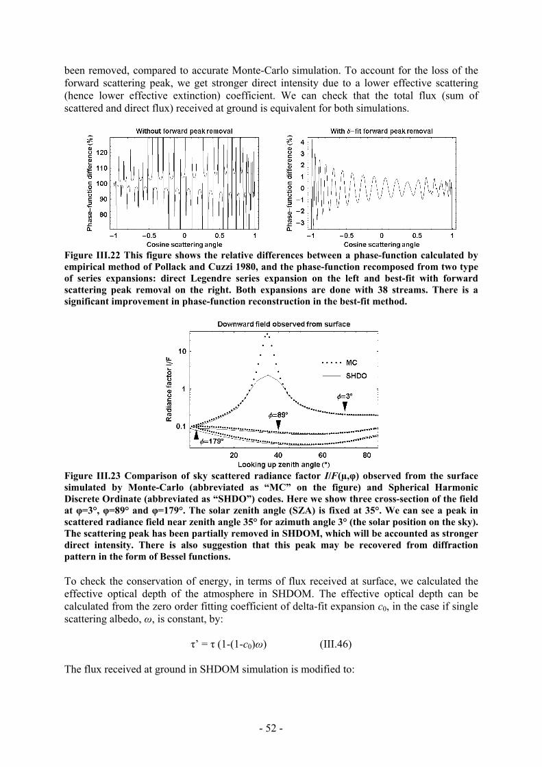
- 52 -

been removed, compared to accurate Monte-Carlo simulation. To account for the loss of the forward scattering peak, we get stronger direct intensity due to a lower effective scattering (hence lower effective extinction) coefficient. We can check that the total flux (sum of scattered and direct flux) received at ground is equivalent for both simulations.

Figure III.22 This figure shows the relative differences between a phase-function calculated by empirical method of Pollack and Cuzzi 1980, and the phase-function recomposed from two type of series expansions: direct Legendre series expansion on the left and best-fit with forward scattering peak removal on the right. Both expansions are done with 38 streams. There is a significant improvement in phase-function reconstruction in the best-fit method.

Figure III.23 Comparison of sky scattered radiance factor I/F(µ,φ) observed from the surface simulated by Monte-Carlo (abbreviated as “MC” on the figure) and Spherical Harmonic Discrete Ordinate (abbreviated as “SHDO”) codes. Here we show three cross-section of the field at φ=3°, φ=89° and φ=179°. The solar zenith angle (SZA) is fixed at 35°. We can see a peak in scattered radiance field near zenith angle 35° for azimuth angle 3° (the solar position on the sky). The scattering peak has been partially removed in SHDOM, which will be accounted as stronger direct intensity. There is also suggestion that this peak may be recovered from diffraction pattern in the form of Bessel functions. To check the conservation of energy, in terms of flux received at surface, we calculated the effective optical depth of the atmosphere in SHDOM. The effective optical depth can be calculated from the zero order fitting coefficient of delta-fit expansion c0, in the case if single scattering albedo, ω, is constant, by:

τ’ = τ (1-(1-c0)ω) (III.46)

The flux received at ground in SHDOM simulation is modified to:

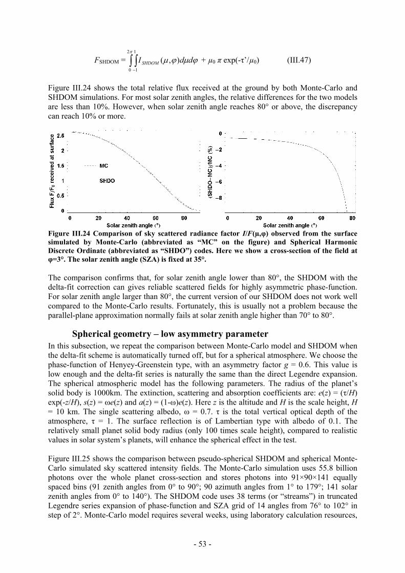
- 53 -

FSHDOM = ∫ ∫−

π

ϕµϕµ2

0

1

1

),( ddI SHDOM + µ0 π exp(-τ’/µ0) (III.47)

Figure III.24 shows the total relative flux received at the ground by both Monte-Carlo and SHDOM simulations. For most solar zenith angles, the relative differences for the two models are less than 10%. However, when solar zenith angle reaches 80° or above, the discrepancy can reach 10% or more.

Figure III.24 Comparison of sky scattered radiance factor I/F(µ,φ) observed from the surface simulated by Monte-Carlo (abbreviated as “MC” on the figure) and Spherical Harmonic Discrete Ordinate (abbreviated as “SHDO”) codes. Here we show a cross-section of the field at φ=3°. The solar zenith angle (SZA) is fixed at 35°. The comparison confirms that, for solar zenith angle lower than 80°, the SHDOM with the delta-fit correction can gives reliable scattered fields for highly asymmetric phase-function. For solar zenith angle larger than 80°, the current version of our SHDOM does not work well compared to the Monte-Carlo results. Fortunately, this is usually not a problem because the parallel-plane approximation normally fails at solar zenith angle higher than 70° to 80°.

Spherical geometry – low asymmetry parameter In this subsection, we repeat the comparison between Monte-Carlo model and SHDOM when the delta-fit scheme is automatically turned off, but for a spherical atmosphere. We choose the phase-function of Henyey-Greenstein type, with an asymmetry factor g = 0.6. This value is low enough and the delta-fit series is naturally the same than the direct Legendre expansion. The spherical atmospheric model has the following parameters. The radius of the planet’s solid body is 1000km. The extinction, scattering and absorption coefficients are: e(z) = (τ/H) exp(-z/H), s(z) = ωe(z) and a(z) = (1-ω)e(z). Here z is the altitude and H is the scale height, H = 10 km. The single scattering albedo, ω = 0.7. τ is the total vertical optical depth of the atmosphere, τ = 1. The surface reflection is of Lambertian type with albedo of 0.1. The relatively small planet solid body radius (only 100 times scale height), compared to realistic values in solar system’s planets, will enhance the spherical effect in the test. Figure III.25 shows the comparison between pseudo-spherical SHDOM and spherical Monte-Carlo simulated sky scattered intensity fields. The Monte-Carlo simulation uses 55.8 billion photons over the whole planet cross-section and stores photons into 91×90×141 equally spaced bins (91 zenith angles from 0° to 90°; 90 azimuth angles from 1° to 179°; 141 solar zenith angles from 0° to 140°). The SHDOM code uses 38 terms (or “streams”) in truncated Legendre series expansion of phase-function and SZA grid of 14 angles from 76° to 102° in step of 2°. Monte-Carlo model requires several weeks, using laboratory calculation resources,

- 54 -

to perform the simulation while the SHDOM complete the computation within 15 minutes on a personal computer. The left panel of Figure III.25 shows a cross-section of the intensity field at azimuth angle equal 3°, 90° and 177° with the SZA in all simulations is 90°. On the right, we see that the two codes agree within 5% for most of scanning looking up zenith angle and for 3 representative solar zenith angles at 85°, 90° and 95°. However when the Sun is near the horizon, the discrepancy becomes significant. This observation is consistent with the fact that the correction ∆θ to the zenith angle relation between layers in the SHDOM is maximum near the horizon direction. This may hints that improvement to SHDOM must include this correction.

Figure III.25 Comparison of sky scattered radiance factor I/F(µ,φ) observed from the surface simulated by Monte-Carlo (abbreviated as “MC” on the figure, shown with error bars) and Spherical Harmonic Discrete Ordinate (abbreviated as “SHDO”) codes. On the left, we show three cuts of the field at φ=3°, φ=90°, φ=177°. The solar zenith angle (SZA) is fixed at 90° and solar azimuth angle at 0°. On the right is the relative difference between results of two methods in %, as function of looking up zenith angle, only for φ=3° but with two more solar zenith angles, namely 85° and 95°. For most of the looking up angles and SZA, the differences lie within 5%. Figure III.26 shows the comparison of flux factor (received flux on ground per initial solar flux F0) as function of solar zenith angles, simulated by spherical Monte-Carlo and pseudo-spherical SHDOM. The SHDOM underestimates the flux, a phenomenon already observed in the parallel-plan case. The relative discrepancy reaches 10% or more at SZA larger than 97°. This means that, in applications of the code SHDOM, we should avoid too large SZA (above 97°) or special care should be taken there.

Figure III.26 Comparison of total received flux factor F/F0 observed from the surface simulated by spherical Monte-Carlo (abbreviated as “MC” on the figure) and pseudo-spherical Spherical Harmonic Discrete Ordinate (abbreviated as “SHDO”) codes. Here F0 is initial solar input flux (input power per perpendicular cross-section area). On the left, we show the flux as functions of

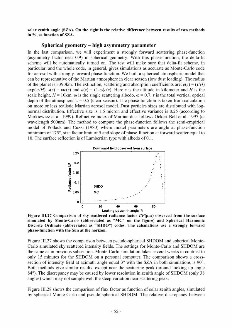
- 55 -

solar zenith angle (SZA). On the right is the relative difference between results of two methods in %, as function of SZA.

Spherical geometry – high asymmetry parameter In the last comparison, we will experiment a strongly forward scattering phase-function (asymmetry factor near 0.9) in spherical geometry. With this phase-function, the delta-fit scheme will be automatically turned on. The test will make sure that delta-fit scheme, in particular, and the whole code, in general, gives simulations as accurate as Monte-Carlo code for aerosol with strongly forward phase-function. We built a spherical atmospheric model that can be representative of the Martian atmosphere in clear season (low dust loading). The radius of the planet is 3390km. The extinction, scattering and absorption coefficients are: e(z) = (τ/H) exp(-z/H), s(z) = ωe(z) and a(z) = (1-ω)e(z). Here z is the altitude in kilometer and H is the scale height, H = 10km. ω is the single scattering albedo, ω = 0.7. τ is the total vertical optical depth of the atmosphere, τ = 0.5 (clear season). The phase-function is taken from calculation on more or less realistic Martian aerosol model. Dust particles sizes are distributed with log-normal distribution. Effective size is 1.6 micron and effective variance is 0.25 (according to Markiewicz et al. 1999). Refractive index of Martian dust follows Ockert-Bell et al. 1997 (at wavelength 500nm). The method to compute the phase-function follows the semi-empirical model of Pollack and Cuzzi (1980) where model parameters are angle at phase-function minimum of 175°, size factor limit of 5 and slope of phase-function at forward-scatter equal to 10. The surface reflection is of Lambertian type with albedo of 0.1.

Figure III.27 Comparison of sky scattered radiance factor I/F(µ,φ) observed from the surface simulated by Monte-Carlo (abbreviated as “MC” on the figure) and Spherical Harmonic Discrete Ordinate (abbreviated as “SHDO”) codes. The calculations use a strongly forward phase-function with the Sun at the horizon. Figure III.27 shows the comparison between pseudo-spherical SHDOM and spherical Monte-Carlo simulated sky scattered intensity fields. The settings for Monte-Carlo and SHDOM are the same as in previous subsection. Monte-Carlo simulation takes several weeks in contrast to only 15 minutes for the SHDOM on a personal computer. The comparison shows a cross-section of intensity field at azimuth angle equal 3° with the SZA in both simulations is 90°. Both methods give similar results, except near the scattering peak (around looking up angle 84°). The discrepancy may be caused by lower resolution in zenith angle of SHDOM (only 38 angles) which may not sample well the steep variation near scattering peak. Figure III.28 shows the comparison of flux factor as function of solar zenith angles, simulated by spherical Monte-Carlo and pseudo-spherical SHDOM. The relative discrepancy between

- 56 -

methods is below 10% for SZA below 95°. For SZA higher than 96°, SHDOM can give severely underestimated radiation field. For more accurate SHDOM simulation, one may consider some modification to the current code, including a spherical correction to zenith angle relation between altitude layers, an interpolation scheme which provide higher resolution near scattering peak and a deeper investigation on the systematic underestimation of total downward flux.

Figure III.28 Comparison of total received flux factor F/F0 observed from the surface simulated by spherical Monte-Carlo (abbreviated as “MC” on the figure) and pseudo-spherical Spherical Harmonic Discrete Ordinate (abbreviated as “SHDO”) codes. Here F0 is initial solar input flux (input power per perpendicular area). On the left, we show the flux as functions of solar zenith angle (SZA). On the right is the relative difference between results of two methods in %, as function of SZA.

3.6 Conclusions Four radiative transfer calculations has been performed for the simulation of ODS signal: Monte-Carlo and Spherical Harmonics Discrete Ordinate models in both parallel-plane and spherical atmosphere. The parallel-plane simulations are useful for daytime dust measurement while calculations in spherical atmosphere are important for twilight clouds. The SHDOM is used for its high computational speed while Monte-Carlo simulation is used to control its accuracy. The Monte-Carlo simulations are shown to be very accurate by validations against known analytic solutions, including extra validation by statistical mechanics. Its major drawback is slow computational speed. The SHDOM model is much more rapid. However, as shown by validations and comparisons to Monte-Carlo simulations, its precision is limited to smaller range of atmospheric models where SHDOM’s approximations hold. In particular, for the spherical atmosphere, the pseudo-spherical SHDOM code is shown to provide acceptable accuracy only for zenith looking angles not too close to the horizon and solar zenith angle not larger than 97°. The codes will be used to investigate the retrieval procedure of the ODS data and its performance in Chapter 4 and applied to terrestrial measurement in Chapter 5. The Monte-Carlo code will be used with representative atmospheric models. Meanwhile, the SHDOM will be used to expand the resolution of the analysis. In this way, we can accelerate the simulation using the fast SHDOM code while controlling its accuracy against Monte-Carlo results in representative cases.

- 57 -

Chapter 4

Simulation of ODS measurements on Mars

4.1 Introduction A set of radiative transfer models in parallel-plane and spherical geometry has been constructed. They will be used in the following for investigating the various aspects of the ODS instrument. Section 4.2 will be dedicated to the simulation of daytime dust measurements and to the characterization of their sensitivity to dust optical depth and particles size distribution. A method will be then explored for retrieving the dust parameters, called χ2 test. Using this method, we are able to estimate the measurement uncertainty on simulated observations with different fields of view and filter configurations. We also analyze the effects of uncertainties of atmospheric parameters not directly retrieved, when varying the working conditions (instrument orientation, solar trajectory and atmospheric opacity). Section 4.3 will provide similar analysis for cloud detection at twilight. Some initial signal simulations are presented first, followed by a definition of the retrieval procedure and an estimation of the theoretical performances regarding the influence of filter configurations and other instrumental and atmospheric parameters.

4.2 Daytime dust measurements In this first section, we will simulate the signal of ODS during the course of the day. We will then analyze the ODS signal’s sensitivity to dust loading and size distributions. Form this study, we will define a retrieval procedure for deriving aerosol optical depth and other atmospheric and instrumental parameters from the anticipated signal. Applying this procedure on simulated measurements, we will investigate the sensitivity of ODS to field of view, filters and other parameters.

4.2.1 Simulation of measurements

Models and controls The atmospheric models for all simulations in this section have the following characteristics. The scattering and absorption coefficients, s0 and a0, vary exponentially with altitude following the expression s = s0 exp(-z/H) and a = a0 exp(-z/H). Here H is the scale height, set at 10 km. The phase-function and single scattering albedo are calculated by the Mie theory (van de Hulst 1981) from a dust ensemble with a log-normal distribution and a refractive index given by Ockert-Bell et al. 1997. The effective size of dust is allowed to vary between 0.6 µm and 4 µm, while the range of effective variance is 0.1 to 5. These ranges cover the typical values, 1.6µm and 0.25, retrieved by Markiewicz et al. 1999. The total optical depth of the atmosphere is varied between 0 and 5, covering both clear seasons (typical optical depth of 0.2 to 0.5) and dust storm conditions (optical depth reaching 4 to 5). We simulate the sky scattered intensity field, corresponding to each atmospheric model, with a radiative transfer code in parallel-plane geometry. The parallel-plane approximation is adequate for solar zenith angle less than 80° (as shown in Chapter 3) and so is suitable for simulating daytime measurement. Using parallel-plane calculations instead of spherical one reduces significantly the duration of calculation. The Monte-Carlo code is used for a sparse grid of representative atmospheric parameters while the SHDOM code is used on more detailed grid to achieve calculation time efficiency. The SHDOM results will be compared to

- 58 -

Monte-Carlo simulations for several representative cases. Usually, SHDOM give the same signal shape as Monte-Carlo simulation but two results differ slightly by a factor of multiplication depending on the solar zenith angle. This multiplication factor will be computed by comparing SHDOM and Monte-Carlo result at the sparse and representative parameter grid. It will be then linearly interpolated at other parameters grid points where there are only SHDOM results. The sky intensity calculated by Monte-Carlo or SHDOM code is later integrated into flux within the nominal annular field of view of ODS with half-angle from 30° to 50°.

Sensitivity to Optical depth Figure IV.1 shows the relation between simulated fluxes received by ODS and atmospheric optical depth. When the Sun is within the field of view (left panel), the flux is the sum of direct and scattered sunlight, which reduces exponentially with optical depth varying from 0 to 5. When the Sun is outside field of view (right), only scattered sunlight is observed, which is maximum around an optical depth of about 2.

Figure IV.1. Relation between total flux received by ODS and aerosol optical depth (τ). On the left is total flux (direct and scattered) when the sun is within the field of view (FOV). On the right is scattered sunlight only when Sun is outside the FOV. Figure IV.2, IV.3 and IV.4 show the evolution of the flux during the course of the day for three typical Sun trajectories across the field of view (FOV) of the instrument, and for a dust optical thickness varying from 0.2 to 5.0. The sun trajectory over the annular FOV is displayed on the left of each figure.

- 59 -

Figure IV.2. Simulated daytime ODS signal. The figure on the left shows the solar trajectory over the sky (gray line), relative to the ODS FOV (white annular disk from 30° to 50°). The left panel shows the flux evolution during the course of the day. In the canonical situation of Figure IV.2, the Sun alternatively crosses the field of view and the central mask. At high latitude or mid-latitude in the winter, or if the instrument is tilted, the solar trajectory relative to the field of view degenerates into the case shown in Figure IV.3 (sun never crossing the central mask) and Figure IV.4 (sun never in the FOV).

Figure IV.3. Same as Figure IV.2, but for a sun never passing through the central mask. Throughout the cases showed, we see that the shape of the ODS daytime signal depends significantly on the aerosol loading. However, the change of shape is less pronounced in the case where the Sun never passes through the field of view (FOV).

- 60 -

Figure IV.4. Same as Figure IV.2, but for a sun never passing in the FOV.

Sensitivity to size distribution of dust particles Figure IV.5 shows the ODS signal for the canonical solar trajectory for a range of dust effective size (on the left) and effective variance (on the right).

Figure IV.5. Dependence of ODS signal on effective size (left) and effective variance (right) of dust size distribution. The direct sunlight is almost unaffected by the variation of dust size parameters. The scattered light decreases at increasing dust size and at increasing effective variance. The two parameters have very similar signatures. They could hardly be separated. Fortunately, when comparing Figure IV.5 to Figure IV.2, we see that both effective size and effective variance affect the signal’s shape very differently from the optical depth. This means that we may be able to invert the optical depth from ODS signal without much interference from uncertainty on aerosol size distribution.

4.2.2 Retrieval procedure In principle, the dust optical depth could be retrieved easily from the direct sunlight alone by the Beer’s law. However, the results will be highly sensitive to the calibration of the instrument and moreover to its potential drift because of dust deposition, temperature dependences and aging. A better method is to look at the change between scattered and total

- 61 -

light, providing a relative measurement of dust optical depth and other atmospheric parameters, independent of calibration. The central idea of the retrieval procedure is to search the best atmospheric model that gives a simulated ODS output that fit to the measurement. The criterion for a best fit is given by the minimum value of mean squared difference between observations and simulations, or the χ2, defined as:

2

1

2

)()()(1 ∑

=⎟⎟⎠

⎞⎜⎜⎝

⎛ −=

N

i isisio

Nχ (IV.1)

Here o(i) and s(i) are the observed and simulated flux points in the daily curve. N is the total number of daily measurement points. The expression of χ2 use the weighted least square method, where we take the assumption that uncertainty of measurement of flux is proportional to the flux. In fact one can calculate the χ2, directly from ODS output signal, O(i) and S(i), which is proportional to logarithm of flux.

( )2

1

2 )()(1 ∑=

−=N

i

iSiON

χ (IV.1)

This retrieval procedure uses all available data points collected during the day. It uses the form of daily measurement, instead of absolute value of independent data points. It is thus insensitive to instrument calibration. This method supports various degenerated measurement cases such as during days when the Sun does not cross the field of view. It also provides estimations of atmospheric parameters other than dust optical depth, such as dust size.

Look-up table of sky intensity fields Since the simulation of the radiative transfer of sunlight in the Martian atmosphere takes long calculation time, the retrieval procedure is based on the use of pre-built look-up tables to be compared to observations, instead of real-time simulations, during minimum searching of χ2. The look-up table is a table containing simulated ODS outputs for a discrete set of atmospheric parameters. Given a set of parameters, one can interpolate between pre-calculated results in the table to deduce ODS output. Retrieved parameters are: dust optical depth, effective radius of the particles and variance of dust size distribution. Discrete values of these parameters, chosen to well sample the range of variation in realistic atmosphere, results in look-up tables of three dimensions. To save memory space in the look-up table, we only store the sky intensities, for discrete values of solar zenith angle from 0° to 80°, instead of the ODS output. This is because the ODS output also depend upon a number of instrumental setup, such as field of view, and on the solar trajectory on a given day. The number of field of view and solar trajectory setups is infinite, while the ODS output for all of these setups can be derived from a single stored sky intensity. The Monte-Carlo simulation in parallel-plane geometry is used for constructing the sky intensity for each choice of atmospheric parameters in a sparse and representative grid. The SHDOM is used to build more detailed grid of simulated intensity, to gain higher resolution for the look-up table while maintaining affordable calculation time. The parallel-plane geometry is used since the solar zenith angle needed for optical depth retrieval is less than 80°.

- 62 -

Generating output and matching Once the look-up table is built, we can retrieve the best parameters using an iterative procedure described hereafter. We begin by some initial guess. The first step is to generate theoretical ODS outputs for given sets of aerosol parameters. To obtain an ODS output for a particular time of a day, at known solar zenith angle (SZA), the sky intensity field corresponding to the given SZA is convolved with the angular and spectral response of ODS to simulate the light flux received by the photodiode. This flux is then converted into ODS output logarithmic signal using the electronics transfer function. Once, an ODS output is calculated for the whole day, the next step of the retrieval procedure is the comparison between the calculated output and the observations. This comparison is realized through the calculation of χ2 which is a function of observation, o(t), and simulations, s(t), along a full day or half day, and possible drift of sensitivity or attenuation by dust deposition (∆V) and local time uncertainties (∆t):

χ2(s, ∆V, ∆t) = Σ(o(ti + ∆t) + ∆V – s(ti))2 (IV.2) The smaller the χ2, the better simulated ODS output resembles the observation. We then change slightly the aerosol parameters and repeat the calculation then change slightly ∆V and ∆t and calculate χ2. If the new χ2 value is smaller, we continue to change the parameters in the same direction. Otherwise, we search another direction. The procedure is repeated until the minimum of χ2 is found on the space of aerosol parameters and ∆V, ∆t. At this minimum of χ2, we have reached the best matching aerosol model as well as instrumental parameters (∆V and ∆t). The details on how to change the parameters in the search of minimum of χ2 is that suggested by Levenberg and Marquardt (Gill et al. 1981). The χ2 test can also provides an estimation of uncertainties on the aerosol parameters from the slope of χ2 valley near the minimum, if the parameters are well de-correlated. This is the case for the aerosol opacity, which is well de-correlated from the other parameters.

0

12 2

2p p

ppχ

−

=

⎛ ⎞∂∆ = ⎜ ⎟

⎜ ⎟∂⎝ ⎠ (IV.3)

Here p is a parameter to be inversed and p0 is the value retrieved of p.

4.2.3 Applications With the retrieval procedure defined above, we can now do some detailed theoretical experiments with a pre-built look-up table and some “fake” observations for various working conditions. The purpose of this analysis is to better understand the sensitivity of the measurement to the field of view, wavelength of its filters, other of atmospheric and instrumental conditions. For quantifying the performances of ODS, we define the uncertainty of retrieval as the standard-deviation of retrieved results from an ensemble of noisy observations. The method is explained in more details below.

Uncertainty evaluation by noisy observation For a given atmospheric model, instrument setting and solar trajectory, we simulate the ODS signal in Volt. The conversion from energy flux to electronics output is done using the measured electronics output function, which can be approximately given by:

O = Log10(0.86 f) + 6.28 (IV.4) Here O is the ODS’s output in Volt, f is the energy power received by photodiode (in W).

- 63 -

The ODS output is then added with a Gaussian noise, (with standard deviation of 0.01V), to generate an ensemble of (1000) different noisy observations. Then, the parameters retrieved for each particular noisy observation are scattered around the reference values. Standard deviations on retrieved results provide an estimation of uncertainty of the inversion. Simulations are performed for three solar trajectories: sun passing through central mask, sun reaching the ODS field of view but never passing through central mask, and sun never in the FOV. The sampling frequency was set uniformly at 1 data point every 15 minutes during daytime. For a given analysis, the flux received by the photodiode is the sky intensity integrated angularly over the given field of view and spectrally over the given filter configuration.

Influence of field of view We first apply the above method for estimating the ODS performance with the two fields of view defined for the NETLANDER and Pascal missions: conical of opening of 30° and annular between 25° to 50°. Two “fake” observations are chosen for two representative optical depth cases: normal low dust loading (τd=0.5, effective size reff = 2µm and effective size variance σeff=0.25) and dust storm condition (τd=4.5, effective size reff = 1.6µm and effective size variance σeff=0.3). The instrumental noise is modeled by a Guassian distribution with a standard deviation of 0.01V. The number of observations in the noisy ensemble is 1000. The center and band-pass of ODS filters are varied between 300 and 1100 nm.

Season % Uncertainty FOV 30° FOV 25°-50°

∆τd/__

dτ (%) 1.47 0.74

∆reff/___

effr (%) 5.4 3.2

Clear (τd = 0.5)

∆σeff/____

effσ (%) 42 13

∆τd/__

dτ (%) 0.2 0.14

∆reff/___

effr (%) 0.8 0.9

Dusty (τd = 4.5)

∆σeff/____

effσ (%) 2.2 2.8

Table IV.1. Percent uncertainty of retrieved aerosol opacity, τd, effective particle size, reff, and effective variance of size distribution, σeff, for a 0.01 V noise in the ±3V signal range. Table IV.1 shows the retrieved relative uncertainties of Martian dust parameters for the two fields of view when solar trajectory passes the zenith (the cases where two fields of view gives their distinctive typical observations) and in the filter configuration of 350 ± 100 nm in one channel and 800 ± 50nm in the other. The annular FOV is much better in giving more accurate dust optical depth. This is mainly because this type of field of view provides additional scattered flux observation in the middle of the day which better constraint the retrieval results than merely scattered flux at high SZA. Furthermore, the Sun can pass through this field of view at higher SZA, helping ODS to work with larger range of orientation and latitude. For these reasons, this field of view was chosen for the ODS

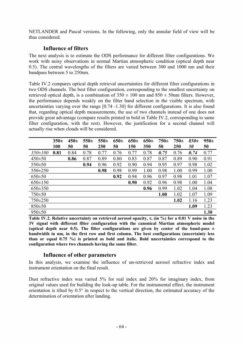
- 64 -

NETLANDER and Pascal versions. In the following, only the annular field of view will be thus considered.

Influence of filters The next analysis is to estimate the ODS performance for different filter configurations. We work with noisy observations in normal Martian atmospheric condition (optical depth near 0.5). The central wavelengths of the filters are varied between 300 and 1000 nm and their bandpass between 5 to 250nm. Table IV.2 compares optical depth retrieval uncertainties for different filter configurations in two ODS channels. The best filter configuration, corresponding to the smallest uncertainty on retrieved optical depth, is a combination of 350 ± 100 nm and 850 ± 50nm filters. However, the performance depends weakly on the filter band selection in the visible spectrum, with uncertainties varying over the range [0.74 -1.30] for different configurations. It is also found that, regarding optical depth measurements, the use of two channels instead of one does not provide great advantage (compare results printed in bold in Table IV.2, corresponding to same filter configuration, with the rest). However, the justification for a second channel will actually rise when clouds will be considered. 350±

100 450± 50

550± 50

550± 250

650± 50

650± 150

650± 350

750± 50

750± 250

850± 50

950± 50

350±100 0.81 0.84 0.78 0.77 0.76 0.77 0.78 0.75 0.76 0.74 0.77 450±50 0.86 0.87 0.89 0.80 0.83 0.87 0.87 0.89 0.90 0.91 550±50 0.94 0.96 0.92 0.90 0.94 0.95 0.97 0.98 1.02 550±250 0.98 0.98 0.99 1.00 0.98 1.00 0.99 1.00 650±50 0.92 0.94 0.96 0.97 0.98 1.01 1.07 650±150 0.90 0.92 0.96 0.98 1.00 1.04 650±350 0.96 0.99 1.02 1.04 1.08 750±50 1.00 1.02 1.07 1.09 750±250 1.02 1.16 1.23 850±50 1.09 1.23 950±50 1.30

Table IV.2. Relative uncertainty on retrieved aerosol opacity, τ, (in %) for a 0.01 V noise in the 3V signal with different filter configuration with the canonical Martian atmospheric model (optical depth near 0.5). The filter configurations are given by center of the band-pass ± bandwidth in nm, in the first row and first column. The best configurations (uncertainty less than or equal 0.75 %) is printed as bold and italic. Bold uncertainties correspond to the configuration where two channels having the same filter.

Influence of other parameters In this analysis, we examine the influence of un-retrieved aerosol refractive index and instrument orientation on the final result. Dust refractive index was varied 5% for real index and 20% for imaginary index, from original values used for building the look-up table. For the instrumental effect, the instrument orientation is tilted by 0.5° in respect to the vertical direction, the estimated accuracy of the determination of orientation after landing.

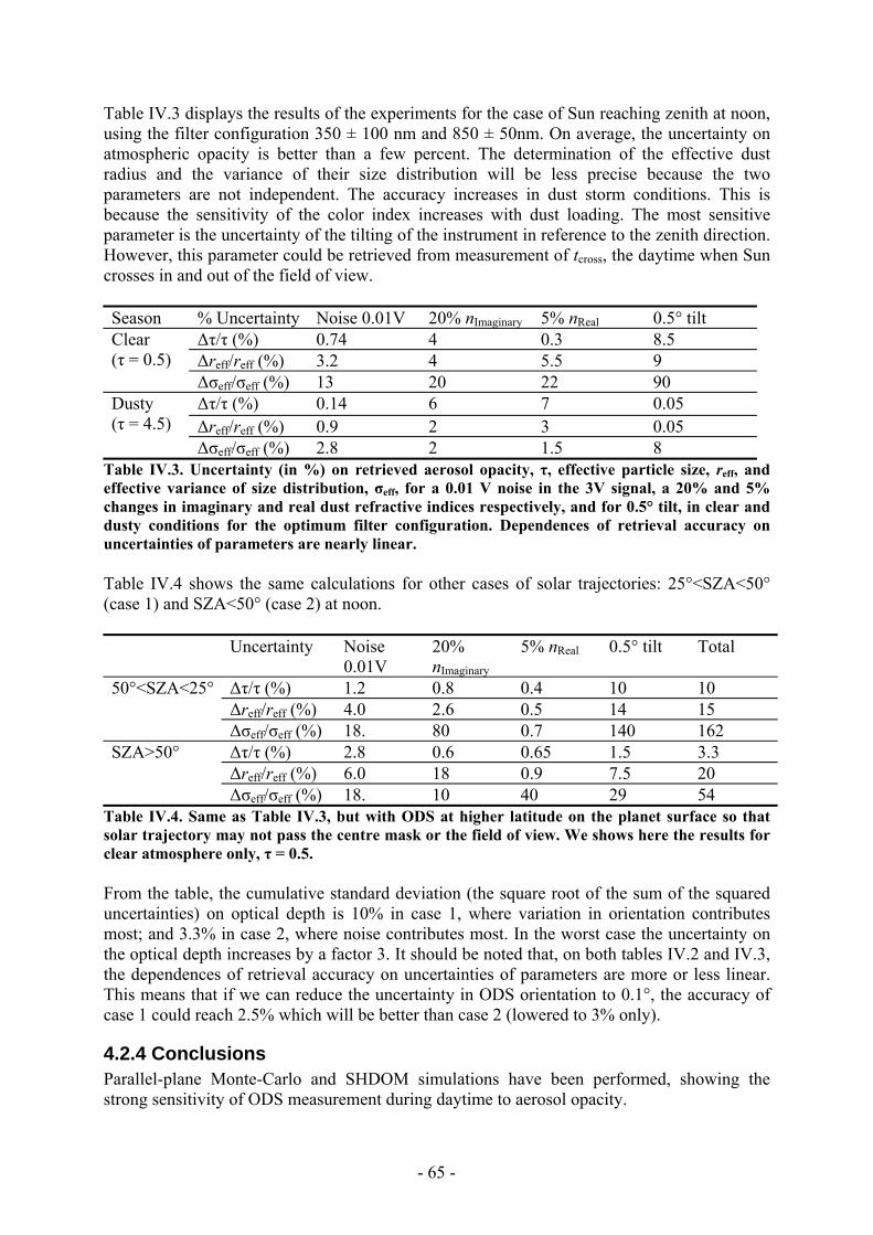
- 65 -

Table IV.3 displays the results of the experiments for the case of Sun reaching zenith at noon, using the filter configuration 350 ± 100 nm and 850 ± 50nm. On average, the uncertainty on atmospheric opacity is better than a few percent. The determination of the effective dust radius and the variance of their size distribution will be less precise because the two parameters are not independent. The accuracy increases in dust storm conditions. This is because the sensitivity of the color index increases with dust loading. The most sensitive parameter is the uncertainty of the tilting of the instrument in reference to the zenith direction. However, this parameter could be retrieved from measurement of tcross, the daytime when Sun crosses in and out of the field of view. Season % Uncertainty Noise 0.01V 20% nImaginary 5% nReal 0.5° tilt

∆τ/τ (%) 0.74 4 0.3 8.5 ∆reff/reff (%) 3.2 4 5.5 9

Clear (τ = 0.5)

∆σeff/σeff (%) 13 20 22 90 ∆τ/τ (%) 0.14 6 7 0.05 ∆reff/reff (%) 0.9 2 3 0.05

Dusty (τ = 4.5)

∆σeff/σeff (%) 2.8 2 1.5 8 Table IV.3. Uncertainty (in %) on retrieved aerosol opacity, τ, effective particle size, reff, and effective variance of size distribution, σeff, for a 0.01 V noise in the 3V signal, a 20% and 5% changes in imaginary and real dust refractive indices respectively, and for 0.5° tilt, in clear and dusty conditions for the optimum filter configuration. Dependences of retrieval accuracy on uncertainties of parameters are nearly linear. Table IV.4 shows the same calculations for other cases of solar trajectories: 25°<SZA<50° (case 1) and SZA<50° (case 2) at noon. Uncertainty Noise

0.01V 20% nImaginary

5% nReal 0.5° tilt Total

∆τ/τ (%) 1.2 0.8 0.4 10 10 ∆reff/reff (%) 4.0 2.6 0.5 14 15

50°<SZA<25°

∆σeff/σeff (%) 18. 80 0.7 140 162 ∆τ/τ (%) 2.8 0.6 0.65 1.5 3.3 ∆reff/reff (%) 6.0 18 0.9 7.5 20

SZA>50°

∆σeff/σeff (%) 18. 10 40 29 54 Table IV.4. Same as Table IV.3, but with ODS at higher latitude on the planet surface so that solar trajectory may not pass the centre mask or the field of view. We shows here the results for clear atmosphere only, τ = 0.5. From the table, the cumulative standard deviation (the square root of the sum of the squared uncertainties) on optical depth is 10% in case 1, where variation in orientation contributes most; and 3.3% in case 2, where noise contributes most. In the worst case the uncertainty on the optical depth increases by a factor 3. It should be noted that, on both tables IV.2 and IV.3, the dependences of retrieval accuracy on uncertainties of parameters are more or less linear. This means that if we can reduce the uncertainty in ODS orientation to 0.1°, the accuracy of case 1 could reach 2.5% which will be better than case 2 (lowered to 3% only).

4.2.4 Conclusions Parallel-plane Monte-Carlo and SHDOM simulations have been performed, showing the strong sensitivity of ODS measurement during daytime to aerosol opacity.

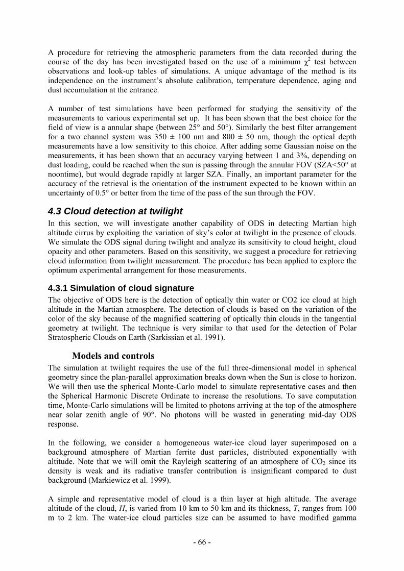
- 66 -

A procedure for retrieving the atmospheric parameters from the data recorded during the course of the day has been investigated based on the use of a minimum χ2 test between observations and look-up tables of simulations. A unique advantage of the method is its independence on the instrument’s absolute calibration, temperature dependence, aging and dust accumulation at the entrance. A number of test simulations have been performed for studying the sensitivity of the measurements to various experimental set up. It has been shown that the best choice for the field of view is a annular shape (between 25° and 50°). Similarly the best filter arrangement for a two channel system was 350 ± 100 nm and 800 ± 50 nm, though the optical depth measurements have a low sensitivity to this choice. After adding some Gaussian noise on the measurements, it has been shown that an accuracy varying between 1 and 3%, depending on dust loading, could be reached when the sun is passing through the annular FOV (SZA<50° at noontime), but would degrade rapidly at larger SZA. Finally, an important parameter for the accuracy of the retrieval is the orientation of the instrument expected to be known within an uncertainty of 0.5° or better from the time of the pass of the sun through the FOV.

4.3 Cloud detection at twilight In this section, we will investigate another capability of ODS in detecting Martian high altitude cirrus by exploiting the variation of sky’s color at twilight in the presence of clouds. We simulate the ODS signal during twilight and analyze its sensitivity to cloud height, cloud opacity and other parameters. Based on this sensitivity, we suggest a procedure for retrieving cloud information from twilight measurement. The procedure has been applied to explore the optimum experimental arrangement for those measurements.

4.3.1 Simulation of cloud signature The objective of ODS here is the detection of optically thin water or CO2 ice cloud at high altitude in the Martian atmosphere. The detection of clouds is based on the variation of the color of the sky because of the magnified scattering of optically thin clouds in the tangential geometry at twilight. The technique is very similar to that used for the detection of Polar Stratospheric Clouds on Earth (Sarkissian et al. 1991).

Models and controls The simulation at twilight requires the use of the full three-dimensional model in spherical geometry since the plan-parallel approximation breaks down when the Sun is close to horizon. We will then use the spherical Monte-Carlo model to simulate representative cases and then the Spherical Harmonic Discrete Ordinate to increase the resolutions. To save computation time, Monte-Carlo simulations will be limited to photons arriving at the top of the atmosphere near solar zenith angle of 90°. No photons will be wasted in generating mid-day ODS response. In the following, we consider a homogeneous water-ice cloud layer superimposed on a background atmosphere of Martian ferrite dust particles, distributed exponentially with altitude. Note that we will omit the Rayleigh scattering of an atmosphere of CO2 since its density is weak and its radiative transfer contribution is insignificant compared to dust background (Markiewicz et al. 1999). A simple and representative model of cloud is a thin layer at high altitude. The average altitude of the cloud, H, is varied from 10 km to 50 km and its thickness, T, ranges from 100 m to 2 km. The water-ice cloud particles size can be assumed to have modified gamma

- 67 -

distribution with effective size of 7 µm and effective variance of 0.1. These values are consistent with those of terrestrial cirrus clouds. However, there are indications from the Thermal Emission Spectrometer (TES) measurement that Martian ice particles are actually smaller (about 2 µm) (Wolf and Clancy 2003). The refractive index of these particles is taken from Warren et al. 1984 (ranging from 1.37 + 4.14 10-9 i at photon wavelength 300 nm to 1.32 + 3 10-6 i at wavelength 1000 nm). The optical depth (at 500 nm) is varied between 0.04 and 0.2. Martian water-ice cloud particles have probably irregular shapes. There are suggestions that these particles are polygonal crystals, (Gooding 1986 or Clancy et al. 2002); however no observation is available on that point. The permanent dust background is fixed to an optical depth of 0.25 (at 500 nm). This corresponds to a clear season on Mars. The dust particle size is assumed to follow a log-normal distribution, with an effective size of 1.6 µm and effective variance of 0.25 (Markiewicz et al. 1999). The refractive index of the dust is taken from Ockert-Bell et al 1997. The dust density decreases exponentially with scale height of 10 km. Although the dust particle shape is irregular, we will assume a spherical shape in the first order analysis. In this analysis, the Mie theory will be used to calculate scattering and absorption coefficients and phase-function of cloud and dust layers. Figure IV.6 and IV.7 show the typical on wavelength dependence of scattering and absorption optical depth and the phase-function of cloud and dust layers respectively. The radiative transfer properties of the cloud layer depend weakly on wavelength, in contrary to that of the dust layer.

Figure IV.6 Wavelength dependence of cloud optical depth (left) and cloud particles’ phase-function (right). The clouds are rather white, with optical characteristics depending weakly on wavelength.

Figure IV.7 Same as Figure IV.6, but for dust particles. The dusts are red, scattering more red light than blue light.

- 68 -

For each test run, the sky intensity field is first calculated, then integrated over the annular field of view between 30° and 50° for deriving the flux received by the ODS photodiode. The flux is finally converted into ODS output in Volt by the equation (IV.4). The following analysis will focus on how the three parameters, optical thickness, average height and geometrical thickness, of Martian water ice clouds affect the ODS output at twilight. The parameters are sampled at a representative grid, where the Monte-Carlo simulation is used, and then expanded at higher resolution, using SHDOM code. In this manner, we can control SHDOM results, fast but less accurate, by Monte-Carlo ones, slow but more precise.

Results of twilight simulations Figure IV.8 shows the evolution of scattered light at zenith during the sunrise period for a pure dust layer without cloud. Note the logarithmic vertical scale in volt. At twilight, the signal jumps by four orders of magnitude within an hour. The scattered light increases at increasing wavelength. This is the result of the wavelength dependence of dust optical depth shown in Figure IV.7.

Figure IV.8 Simulation of ODS output in volts at sunrise for dust only (SZA=90° at 6h). The signal, proportional to the logarithm of received sunlight, varies by 6 orders of magnitude. The intensity increases with wavelength. The sky is red. Figure IV.9 shows of the case of cloud only without dust. The cloud layer is at 35km, with an optical thickness of 0.08 and a geometrical thickness of 4km. The plot shows a bump corresponding to an increased scattered light when the photons reach the cloud tangentially. The spectral dependence is less pronounced than in the case of dust only. This result is consistent with wavelength dependence of cloud optical depth shown in Figure IV.6.

- 69 -

Figure IV.9 Similar to Figure IV.8 but for a water-ice cloud at 35km with an optical thickness of 0.08 and a geometrical thickness of 4km. A bump appears a little before 90° SZA (at 6h) when the cloud is illuminated tangentially. Figure IV.10 shows the result of simulation with both clouds and dust on the left and on the right, the evolution of the color index (CI) that is the logarithm of the ratio between the light scattered at 950 and 350 nm. The dust component is the same as in Figure IV.8 and the cloud component is the one of Figure IV.9. The relative contribution of the cloud to the overall scattered light increases when wavelength decreases. As the sun rises, the CI displays first a blueing (smaller CI) followed by a reddening (larger CI).

Figure IV.10 Left: similar to Figure IV.8 but for an atmosphere of combined dust and cloud. The dust component is the same as in Figure IV.8 and the cloud component is the same as in Figure IV.9. Right: color index (CI) for the same atmosphere. The presence of a cloud results in a blueing followed by a reddening around 90° SZA. Figure IV.11 shows the dependence of the color index on the cloud altitude, geometric and optical thickness. On each figure of Figure IV.11, one parameter is varied from the reference atmosphere of Figure IV.10. The time (or SZA) of the maximum blueing varies with the cloud height, occurring earlier (or at larger SZA) at increasing altitude. The relative amplitude of the reddening increases at decreasing geometrical thickness and at increasing optical thickness. The color index is a good indicator of the cloud height and to a less extend of its geometric and optical thicknesses. This could help retrieving these parameter of Martian cloud from ODS measurement of color index.

- 70 -

Figure IV.11 Color index sensitivity on cloud height (a), geometrical thickness (b) and optical depth (c). In each figures, only one parameter is varied from the reference model with a cloud at 35km of 4km geometrical thickness and 0.08 optical depth.

Conclusions The impact of Martian high altitude clouds on the scattered light observed at zenith by ODS during twilight periods has been simulated with the Monte-Carlo radiative transfer model. At sunrise, the presence of a cloud results in a blueing of the sky for about 10 minutes followed by a significant reddening for about the same duration, the opposite occurring at sunset. The suggested method for deriving cloud properties is the use of a color index, ratio between the light intensity at two wavelengths relatively independent on dust load. The most sensitive parameter in the CI is the cloud’s height which could be derived from the time (SZA) of the maximum blueing, while the optical thickness could be derived from its amplitude.

4.3.2 Retrieval procedure A retrieval procedure of cloud characteristics is proposed, based on the matching of observed CI change with a pre-built look-up table using the χ2 test. This approach is very similar to the procedure used for measuring dust.

Look-up table of color index The first step is to build the look-up table containing CI as function of solar zenith angle (SZA), for discrete values of cloud parameters. Here we will concentrate on two parameters, namely cloud’s height and optical thickness. Unlike the daytime ODS output, the observation at twilight is largely insensitive to the rotational orientation on the horizontal plane of the instrument. This means that the observations can be approximately considered to depend on only solar zenith angle (SZA), hence we can store, in the look-up table, directly ODS output in Volt instead of sky intensity.

(a)

(b) (c)

- 71 -

Sky intensity fields are calculated for SZA from 80° to 100°. The Monte-Carlo model is first used with representative values of cloud parameters and then the Spherical Harmonic Discrete Ordinate for increasing the resolution. A “normalized CI”, the CI normalized at the maximum of reddening (just after the peak of blueing) will be used instead of the CI itself for removing the CI dependence on the calibration of the instrument. The use of such normalized CI thus provides a relative measurement. Discrete values of cloud parameters are chosen to well sample the expected variation of Martian cloud characteristics. The altitude is varied from 10 km to 50 km while the optical thickness ranges from 0.001 to 0.1.

Generating output and matching Once the look-up table is built, the retrieval procedure consists of searching the cloud parameters that generate CI curve best matching observation. Given a set of cloud parameters, the CI curve is generated by interpolating between curves in the look-up table. The search for the best match is based on minimizing the expression:

χ2(s, ∆V) = Σ(o(szai) + ∆V – s(szai))2 (IV.5) Here o(sza) is the observation as function of SZA , s(sza) is the simulation, ∆V is the shift of signal. This method is similar to what presented in 4.2.2 and will not be repeated here.

4.3.3 Applications As in the case of dust, a number of test runs has been performed to explore the sensitivity of the retrievals to instrumental set ups and evaluate their accuracy after addition of noise in the measurements. Since the sun is always outside the FOV, CI measurements at twilight are independent of the definition of the FOV. The most important parameter here is the choice of filters.

Influence of filters The following test runs have been carried with a cloud layer at 35 km of a 0.08 optical depth. A Gaussian noise of 0.01V standard deviation has been added. Table IV.5 shows the precision (standard deviation) of retrieved clouds altitude and optical thickness, for different choice of filters. Filter 1 Filter 2

350±50nm 800±50nm

350±50nm 700±50nm

350±50nm 500±50nm

500±50nm 800±50nm

500±50nm 700±50nm

700±50nm 800±50nm

∆τc/τc (%) 1.8 1.9 2.8 5.1 3.7 6.7 ∆hc/hc (%) 0.4 0.41 0.46 1.9 1.5 2.7

Table IV.5. Relative uncertainty on retrieved cloud opacity, ∆τc, and cloud height, ∆hc, when observation are added with noise of 0.01V over ±3V output, for different filter configurations. In the case of the cloud retrieval, the best arrangement for the filters was found to be 350 ± 50nm and 800 ± 50nm.. The best results could be obtained by narrowing the band-pass of the UV filter. This result agrees with preliminary analysis suggesting that the color index amplifies with the wavelength separation of the two channels.

- 72 -

Influence of un-retrieved parameters The influence of un-retrieved parameters (dust opacity, dust effective size, dust effective size variance, cloud geometrical thickness, cloud effective size and cloud effective size variance) on height and optical thickness retrievals has also been explored in the optimum 350-800 nm filter configuration. Table IV.6 shows the deviation of results when the un-retrieved parameters are change by 1% from reference cloud at 35km with optical depth of 0.08. Note that the deviations depend approximately linearly on the parameter variation and can be extrapolated for other change of parameters.

Uncertainty 1%τd 1%reff-d 1%σeff-d 1%dc 1%reff-c 1%σeff-c ∆τc/τc (%) 0.3 0.4 0.1 0.006 0.3 0.06 ∆hc/hc (%) 0.5 0.006 0.01 0.002 0.2 0.002

Table IV.6. Uncertainty on retrieved cloud opacity, ∆τc, and cloud height, ∆hc, for one percent change of dust opacity, τd, dust effective size, reff-d, dust effective variance, σeff-d, cloud thickness, dc, cloud effective size, reff-c and cloud effective variance, σeff-c. Most sensitive parameters are dust opacity and effective size, when present at the altitude of the cloud layer, and cloud particles effective size. The cloud geometric thickness has little impact. However, since in the dust layer in the atmosphere layer is confined to the lower layers and the clouds are located above 20 km, the interference between the two will be very limited. The only remaining sensitive parameter will be then cloud particle effective size. The proposal is to include this parameter in a further improved retrieval.

4.3.4 Conclusions Monte-Carlo and SHDOM simulations in spherical geometry have been performed for investigating the sensitivity of ODS color index (CI) measurements during twilight periods to Martian cirrus altitude and opacity. The CI was found to be extremely sensitive to the presence of high altitude clouds resulting in a blueing followed by a reddening of the zenith sky at sunrise (the opposite at sunset). A retrieval procedure based on the comparison of observations to a set of look-up tables of by a χ2 test is suggested. The method has been applied to explore the sensitivity of the measurements to the experimental arrangement as well as to dust and clouds parameters and evaluating the anticipated precision of the retrievals. The most important instrumental parameter was found to be the choice of color filters characteristics. The best arrangement is the use of relatively narrow filters of 50 nm band pass centered as far as possible at 350 and 800 nm. The choice of FOV has little impact. Providing the cloud is above the dust layer (e.g. above 20 km), its altitude could be retrieved to within ± 150m and its opacity to within 10%. Another sensitive parameter, the cloud particles effective size not included in the current retrieval algorithm, has been identified which is suggested to be included in a further version.

4.4 Conclusions Model simulations fully confirm the ability of the ODS instrument to measure the dust opacity and the high altitude clouds of the atmosphere of Mars.

- 73 -

Dust opacity measurements, independent of calibration changes, could be best performed by looking at the evolution of the signal when the sun is passing across the field of view of the instrument. A FOV of annular (25°-50°) shape providing zenith sky measurements around noontime was found superior to a conical shape. The wavelength of observations is not crucial. A retrieval procedure based on the comparison of the measurements during a full day to look-up tables pre-constructed with parallel-plane radiative transfer codes by a χ2 test, is being proposed. Test runs using this method have shown that an accuracy of 1-3% on dust opacity could be reached. The most sensitive parameter influencing the retrieval is the tilting of the instrument, which must be known to within ± 0.5°. This parameter is expected to be determined to a high degree of accuracy from long series of measurements of time of Sun’s crossing the edge of the FOV at varying sun declination. Clouds could be detected by looking at the evolution of the color of the sky at twilight. Model simulations carried with the Monte-Carlo and the SHDOM in spherical geometry, mandatory at large SZA, show that the sky color index (CI) is extremely sensitive to the presence of high altitude clouds. The most important instrumental parameter was found to be the choice of color filters characteristics. The best arrangement is the use of relatively narrow filters of 50 nm band pass centered as far as possible at 350 and 800 nm. The choice of FOV has little impact. A retrieval procedure based on the use of a look-up table and a χ2 optimization similar to that proposed for dust opacity has been developed with which the performances of cloud detection by the color index method has been investigated. Providing the cloud is above the dust layer (e.g. above 20 km), it was shown that its altitude could be retrieved to within ± 150m and its opacity to within 10%. Although not introduced in the retrieval process, the cloud particles effective size was also found to play a role. It is suggested to introduce this parameter in a further development. Next step is to understand how well the above conclusions could be supported by real observations. The next chapter will deal with this validation aspects by comparisons performed in the Earth’s tropic next to a CIMEL – AERONET photometer for dust optical thickness and in the frequent presence of high altitude cirrus clouds over the area for clouds detection.

- 74 -

Chapter 5

Validation of ODS on the Earth

5.1 Introduction The approach for validating the concept, the experimental arrangement as well as the simulation models of ODS was to carry a series of measurements on the Earth at a location where atmospheric conditions could be as far as possible similar to those of Mars. The location selected for that is Ouagadougou in Burkina-Faso in the Sahelian region where strong Saharian dust episodes are frequently reported during the winter (Hsu et al., 1999), as well as cirrus clouds near the tropopause around 16 km. The other advantage of the location is the presence of a CIMEL AERONET photometer to which the ODS dust opacity measurements could be directly compared. An ODS scientific model very similar to the space version was deployed there in November 2004 for at least 6 months operations. The experimental arrangement, the results of the measurements and of their comparison to the CIMEL photometers are described below.

5.2 ODS scientific models Two scientific versions of the NETLANDER prototypes with their Ground Support Equipments (GSE) have been built. As said above the first has been installed at Ouagadougou and the second close to a mini-lidar at Palaiseau in France next to our laboratory not very convenient for aerosol measurements in the winter, but for long duration environmental testing. Only the measurements of Ouagadougou will be used in the following.

5.2.1 Experimental setup The main component of the ODS scientific model is identical to the space prototype but complemented by a number sub-systems for requirement of autonomous operation on the Earth. The additions include: 1. A glass dome to protect the optical head from rain, snow, dust and insect. 2. An electronics box equipped with ventilator to help maintain ambiance temperature in desert working condition. 3. Ground Supporting Equipments (GSE): adapt main AC power supply to DC source for ODS electronics, program the ventilator and connect ODS output to input of digitization. 4. A Data Acquisition (DAQ) Hardware digitizes ODS output to computer readable signal (through USB connection). 5. A PC computer with a LabView software automatically receives and stores ODS output to local hard drive and, in parallel, repeatedly establishes internet connection and send daily data to our laboratory’s FTP (File Transfer Protocol) server. 6. Uninterruptible Power Supply (UPS) providing power for the whole data acquisition chain from possibly unstable local electric supply. The glass domes, in the form of hemisphere, are manufactured in Service d'Aeronomie, CNRS, France, from glass transparent in the range 300nm to 1000nm. The dome should not affect the spectral band of ODS but change slightly the ODS field of view due to small in-homogeneity of thickness. Therefore the scientific versions have all passed measurement of

- 75 -

field of view described previously for the space model. To prevent condensation of water vapor, the dome is closed firmly by plastic joins and dry silicate (a mineral that absorb water vapor) is placed inside. Three independent LabView programs were developed for the data acquisition. The first is for data reception and storage, the second is for data transmission and the third is to enable remote connection and, if possible and required, modification of the settings of the ODS computer from the laboratory. For data transmission, we preview both local network and telephonic with either fixed or dynamic IP address types. All three programs were planed to run permanently and in parallel. Further, they can communicate with the UPS (Uninterruptible Power Supply). If the main power source is cut off for long time that energy stored in UPS runs out, the UPS can give a warning signal to the computer and the three programs can safely save data and automatically turn off. They are automatically turned on when the power returns.

5.2.2 Desert dust and cirrus clouds at the tropics The ODS was installed in November 2004 at the Institut de Recherche en Sciences Appliquées et Technologies (IRSAT), in the outskirt of the city, next to the AERONET CIMEL photometer, at 12°11’59’’ N and 1°23’59’’ W. Figure V.1 shows the experimental set up on the terrace of the building. The ground-support equipment is installed in the office beneath as shown on Figure 2. After testing, the instrument was left running automatically; the only human interventions to perform is the cleaning of the dome, the replacement of the dome’s silicate when needed and a daily check of operations displayed on the screen of the computer. The data are both stored on the hard disk of the computer and transmitted by the Internet to the laboratory in France.

Figure V.1. ODS at Ouagadougou. The optical head is protected by the glass dome. The electronics is inside the aluminum box just underneath. The ODS is fixed firmly to a pile of bricks below. The dust collector on the right is a passive copy of ODS optics to see how much dust could deposit after a long period of exposure. The CIMEL photometer is on the forefront. The installation proved to be satisfactory. The instrument performed smoothly until June 2005, at the exception of periods of power breakdown, but after which it always restarted properly. Because of frequent and sometimes long interruptions of the Internet link, the data

ODS dust collector

- 76 -

could not always be transmitted daily as foreseen, but could be always recovered afterwards from the hard disk.

Figure V.2. Indoor acquisition chain. (1): the UPS (Uninterruptible Power Supply), (2): the GSE (Ground Supporting Equipments), (3): the DAQ (Data Acquisition Hardware), (4): Computer showing LabView interface.

5.3 Experimental results Figure V.3 shows a typical day of ODS measurements in cloud free conditions, on 23 December 2004, when the aerosol optical depth was smaller than 0.5. Displayed are the signals of the two channels (red channel signal displayed in solid line, blue channel in dotted) at the output of the logarithmic amplifier (1.2 volt equivalent to a flux change of one decade) and the color index (thin grey line) derived from the ratio between the two channels.

Figure V.3. ODS measurement at Ouagadougou on 23 December 2004, typical of dust and cloud free day. As the sun rises, the signal of both channels first rapidly increases within 40 minutes and then slower until the sun enters into the annular FOV between 50° and 25° SZA for two hours, between 9:30 and 11:30. Around noon the detector is shadowed by a branch supporting the

11

22

33

44

- 77 -

central mask, intentionally oriented to the South direction. The signal thus drops for half an hour. The evolution during the afternoon is almost symmetric to that of the morning with the sun within the FOV between 12:15 and 14:15. Some noise could be seen during direct sun periods due to small changes of atmospheric transmission. Small variations could be also seen in the scattered light in the afternoon due to the presence of small thin clouds drifting within the FOV. The signal drops rapidly by several orders of magnitude at sunset. The step at the beginning of the night is due to the presence of the full moon in the FOV, resulting in a signal similar to that of the sun during daytime but of amplitude lesser by 4-5 orders of magnitude. The signal then decreases during the night for two reasons: the setting of the moon, which could be seen around 3:30 am on the previous morning and the night-time cooling of the detector sensitive at very low levels below the normal threshold of measurements indicated by a horizontal bar. Also displayed in Figure V.3 is the color index that is the ratio between red and blue channels. A diurnal variation could be observed: bluer sky (smaller CI) at low sun, reddening during the pass of the sun or the moon within the FOV, as well as bumps at SZA >90° indicated by vertical bars, during twilight periods. These are the signatures of the presence or thin cirrus clouds in the upper troposphere. However, the desert atmospheric dust loading varies greatly from day to day at Ouagadougou. Figure V.4 shows a typical day, 7 January 2005, of large dust loading when the opacity could be as large as 4. No more change could be observed when the sun passes in the ODS FOV. However, the cirrus could be still seen at twilight. The dust in the lower atmosphere is in the darkness and has small impact on the color index variation at twilight. Also seen on that day is the presence of some spikes in the evening, which could be due to an electromagnetic interference or some light in the surroundings.

Figure V.4. Same as Figure V.3 but on 7 January 2005, a day of large dust load. No more increase could be observed when the sun pass in the ODS FOV. Some spikes could be observed in the evening in the red channel which might be due either to an interference or car lights in the surroundings. Though fortunately infrequent, there are also overcast days where the signal differs greatly, making the retrieval much more difficult. Figure V.5 shows an example of such day on

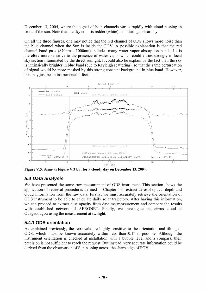
- 78 -

December 13, 2004, where the signal of both channels varies rapidly with cloud passing in front of the sun. Note that the sky color is redder (white) than during a clear day. On all the three figures, one may notice that the red channel of ODS shows more noise than the blue channel when the Sun is inside the FOV. A possible explanation is that the red channel band pass (870nm - 1000nm) includes many water vapor absorption bands. Its is therefore more sensitive to the presence of water vapor which could varies strongly in local sky section illuminated by the direct sunlight. It could also be explain by the fact that, the sky is intrinsically brighter in blue band (due to Rayleigh scattering), so that the same perturbation of signal would be more masked by this strong constant background in blue band. However, this may just be an instrumental effect.

Figure V.5. Same as Figure V.3 but for a cloudy day on December 13, 2004.

5.4 Data analysis We have presented the some raw measurement of ODS instrument. This section shows the application of retrieval procedures defined in Chapter 4 to extract aerosol optical depth and cloud information from the raw data. Firstly, we must accurately retrieve the orientation of ODS instrument to be able to calculate daily solar trajectory. After having this information, we can proceed to extract dust opacity from daytime measurement and compare the results with established network of AERONET. Finally, we investigate the cirrus cloud at Ouagadougou using the measurement at twilight.

5.4.1 ODS orientation As explained previously, the retrievals are highly sensitive to the orientation and tilting of ODS, which must be known accurately within less than 0.1° if possible. Although the instrument orientation is checked at installation with a bubble level and a compass, their precision is not sufficient to reach the request. But instead, very accurate information could be derived from the observation of Sun passing across the sharp edge of FOV.

- 79 -

Orientation retrieval The ODS orientation is defined in a local coordinate system {x,y,z} where z is the zenith, x is in the East direction, y is in the North direction. The instrument viewing directions are {x’,y’,z’} with z’ is the ODS vertical axis (the symmetry axis of ODS mirrors), x’ is the direction from mirror center towards the ODS cable connection and y’ is perpendicular to both x’ and z’ by right hand rule. The orientation of an ODS track can be characterized by 3 numbers: ∆θ, ∆φ and Φ. Here ∆θ is the angle between z’ and z. We know that ∆θ is small, limited to few degrees as ODS is installed toward the zenith. ∆φ is the azimuth angle of ODS vertical axis z’ in reference system {x,y,z}. Φ is the angle between x’ and x. For two ODS channels there are in total 5 numbers to be determined: ∆θ1, ∆φ1, ∆θ2, ∆φ2 and Φ because the direction x’ is the same for both tracks. Here the suffixes 1 is for channel 1 (blue) and 2 is for channel 2 (red). In the preliminary retrieval, we first find the value of Φ with the assumption that ∆θ1 and ∆θ2 are small (less than few degrees): ∆θ1 ≈ 0, ∆θ2 ≈ 0. ODS signal was first simulated with a zero optical depth model (for sharpest transitions at border of FOV) with different trials of Φ, then adjusted to observed transition times. The transitions times are defined as the time at which the second order time derivative of signal is zero. There are 4 transition times: t1 is when the Sun enters the FOV, t2 is the beginning of noon masking, t3 is the ending of noon masking, and t4 is when the Sun leaves the FOV. Figure V.6 shows an example of ODS measurement in the red channel on 10 November 2004 (gray line), fitted with a simulation (black thin line) at the 4 transition times (dashed vertical lines). From the best fits for all cloud free days with aerosol opacity smaller than 0.5 using both channels, we get the best fit value Φ = 94°±0.2°.

Figure V.6. ODS red channel measurements on 10 November 2004 (gray line) with a best fit zero-optical-depth simulation (black line). The fitting parameters are the transition times as shown by the vertical dashed lines. The simulation uses ∆θ1 = 0, ∆θ2 = 0 and value Φ ≈ 94°. In the next step, we find {∆θ1, ∆φ1} and {∆θ2, ∆φ2}. Note that when the viewing directions of two channels are not parallel, the sun enters the field of view of one channel before the other, resulting in a sharp variation of color index. The effect was consistently observed during cloud free days. Figure V.7 shows an example for 10 November 2004 where strong blue shifts could be observed at transitions, caused by difference in orientation of two channels. This can also be seen in color index signal in Figure V.3. The color index signal provides 4 transition times: t1 the time of maximum blue color, t2 the starting time of noon masking (averaged for

- 80 -

both tracks), t3 the end time of noon masking (averaged for both tracks), and t4 the time of maximum blue. The 4 transitions provide 4 equations to determine 4 parameters (Φ is fixed to its preliminary value). Figure V.7 shows an example of best fit of color index. From the statistics for all cloud free days with aerosol opacity lower than 0.5, the best fit values are: ∆θ1 = 2°±0.05°, ∆φ1 = 0°±0.1°, ∆θ2 = 0.8°±0.05°, ∆φ2 = 10°±0.1°. Although the two channels are mounted on the same mechanical structure, their axes differ by 1°, which the above method allows to appreciate to within 0.1°.

Figure V.7. ODS color index measurement on 10 November 2004 (gray line) with a best fit zero-optical-depth simulation for this day (black line). The fitting parameters are the transition times as shown by the vertical dashed lines. The simulation uses Φ = 94° and values ∆θ1 ≈ 2°, ∆φ1 ≈ 0°, ∆θ2 ≈ 0.8°, ∆φ2 ≈ 10°.

Solar trajectory After precisely retrieving the ODS orientation, accurate Sun trajectory relative to ODS field of view for any days during the measurement campaign can be computed. Figure V.8 shows such trajectory at the winter solstice on December 23, 2004. Note that ODS was intentionally oriented approximately with one of its mask supporting branch oriented to the South.

- 81 -

Figure V.8. Sun trajectory over the sky relative to ODS field of view on 23 December 2004 at Ouagadougou. The crossing line is the solar trajectory where the points associated with numbers along the line show the UTC time corresponding to solar positions. The background picture is the ODS field of view where white and black regions correspond to 100% and 0% transmission respectively. Figure V.9 shows the prediction at the end of May 2005 near the summer solstice for the worst case when the sun is masked during most of the day. The orientation of one of the mask supporting branch was not a good idea.

Figure V.9. Prediction of solar trajectory on 31 May 2005.

5.4.2 Dust The main objective of ODS instrument is the daily measurement of atmospheric aerosol and dust opacity. In this section, we will apply the retrieval procedure to find daily dust opacity at Ouagadougou from the measurements. The results will be validated against measurement of an AERONET photometer. Apart from dust optical depth, we also study retrieval of other parameters, such as the long-term instrumental drift.

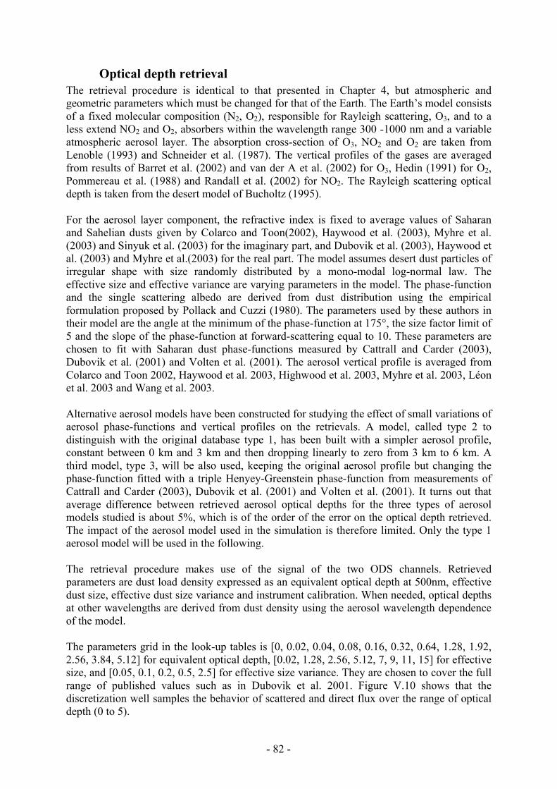
- 82 -

Optical depth retrieval The retrieval procedure is identical to that presented in Chapter 4, but atmospheric and geometric parameters which must be changed for that of the Earth. The Earth’s model consists of a fixed molecular composition (N2, O2), responsible for Rayleigh scattering, O3, and to a less extend NO2 and O2, absorbers within the wavelength range 300 -1000 nm and a variable atmospheric aerosol layer. The absorption cross-section of O3, NO2 and O2 are taken from Lenoble (1993) and Schneider et al. (1987). The vertical profiles of the gases are averaged from results of Barret et al. (2002) and van der A et al. (2002) for O3, Hedin (1991) for O2, Pommereau et al. (1988) and Randall et al. (2002) for NO2. The Rayleigh scattering optical depth is taken from the desert model of Bucholtz (1995). For the aerosol layer component, the refractive index is fixed to average values of Saharan and Sahelian dusts given by Colarco and Toon(2002), Haywood et al. (2003), Myhre et al. (2003) and Sinyuk et al. (2003) for the imaginary part, and Dubovik et al. (2003), Haywood et al. (2003) and Myhre et al.(2003) for the real part. The model assumes desert dust particles of irregular shape with size randomly distributed by a mono-modal log-normal law. The effective size and effective variance are varying parameters in the model. The phase-function and the single scattering albedo are derived from dust distribution using the empirical formulation proposed by Pollack and Cuzzi (1980). The parameters used by these authors in their model are the angle at the minimum of the phase-function at 175°, the size factor limit of 5 and the slope of the phase-function at forward-scattering equal to 10. These parameters are chosen to fit with Saharan dust phase-functions measured by Cattrall and Carder (2003), Dubovik et al. (2001) and Volten et al. (2001). The aerosol vertical profile is averaged from Colarco and Toon 2002, Haywood et al. 2003, Highwood et al. 2003, Myhre et al. 2003, Léon et al. 2003 and Wang et al. 2003. Alternative aerosol models have been constructed for studying the effect of small variations of aerosol phase-functions and vertical profiles on the retrievals. A model, called type 2 to distinguish with the original database type 1, has been built with a simpler aerosol profile, constant between 0 km and 3 km and then dropping linearly to zero from 3 km to 6 km. A third model, type 3, will be also used, keeping the original aerosol profile but changing the phase-function fitted with a triple Henyey-Greenstein phase-function from measurements of Cattrall and Carder (2003), Dubovik et al. (2001) and Volten et al. (2001). It turns out that average difference between retrieved aerosol optical depths for the three types of aerosol models studied is about 5%, which is of the order of the error on the optical depth retrieved. The impact of the aerosol model used in the simulation is therefore limited. Only the type 1 aerosol model will be used in the following. The retrieval procedure makes use of the signal of the two ODS channels. Retrieved parameters are dust load density expressed as an equivalent optical depth at 500nm, effective dust size, effective dust size variance and instrument calibration. When needed, optical depths at other wavelengths are derived from dust density using the aerosol wavelength dependence of the model. The parameters grid in the look-up tables is [0, 0.02, 0.04, 0.08, 0.16, 0.32, 0.64, 1.28, 1.92, 2.56, 3.84, 5.12] for equivalent optical depth, [0.02, 1.28, 2.56, 5.12, 7, 9, 11, 15] for effective size, and [0.05, 0.1, 0.2, 0.5, 2.5] for effective size variance. They are chosen to cover the full range of published values such as in Dubovik et al. 2001. Figure V.10 shows that the discretization well samples the behavior of scattered and direct flux over the range of optical depth (0 to 5).

- 83 -

Figure V.10. Scattered and direct sunlight flux over a range of aerosol optical depth. The flux is given as ODS output signal in the blue channel (in Volt). The scattered light is calculated for a sun at zenith (0° SZA) and the total flux (direct + scattered) for a SZA of 40°. The points show the grid point of look-up table which well sample the variation of the fluxes.

Aerosol optical depth The above procedure of optical depth retrieval had been applied to the measurements at Ouagadougou. Figure V.11 shows two examples of typical best fit between simulations and measurements, for a day (25 November 2004) and a night (25-26 November 2004).

Figure V.11 Fits between theoretical simulations and observations for the day of 25 and the night of 25-26 November 2004. The thin lines are observations while the thick dashed lines are simulations. Figure V.12 shows all available ODS and AERONET daily average aerosol optical depth data at 870nm, the CIMEL photometer longest wavelength channel, between November 2004 and February 2005. The ODS error bars shown by empty boxes correspond to the slope of χ2 valley (see equation IV.3, Chapter 4). The AERONET data are daily averages with error bars being the standard deviation. The days are classified as “cloudy days” and “clear days”. Cloudy days are days where the square root of minimum of χ2 per ODS measurement point exceed 0.1 V. The two

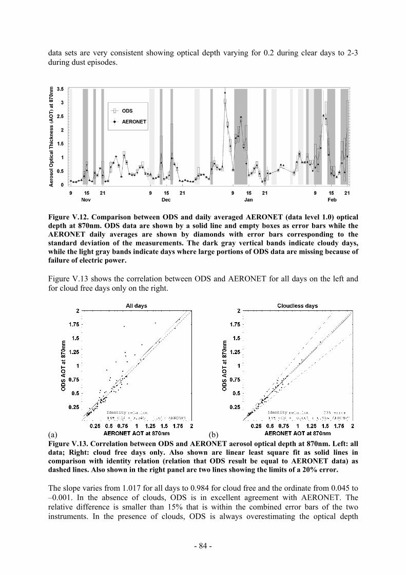
- 84 -

data sets are very consistent showing optical depth varying for 0.2 during clear days to 2-3 during dust episodes.

Figure V.12. Comparison between ODS and daily averaged AERONET (data level 1.0) optical depth at 870nm. ODS data are shown by a solid line and empty boxes as error bars while the AERONET daily averages are shown by diamonds with error bars corresponding to the standard deviation of the measurements. The dark gray vertical bands indicate cloudy days, while the light gray bands indicate days where large portions of ODS data are missing because of failure of electric power. Figure V.13 shows the correlation between ODS and AERONET for all days on the left and for cloud free days only on the right.

(a) (b) Figure V.13. Correlation between ODS and AERONET aerosol optical depth at 870nm. Left: all data; Right: cloud free days only. Also shown are linear least square fit as solid lines in comparison with identity relation (relation that ODS result be equal to AERONET data) as dashed lines. Also shown in the right panel are two lines showing the limits of a 20% error. The slope varies from 1.017 for all days to 0.984 for cloud free and the ordinate from 0.045 to –0.001. In the absence of clouds, ODS is in excellent agreement with AERONET. The relative difference is smaller than 15% that is within the combined error bars of the two instruments. In the presence of clouds, ODS is always overestimating the optical depth

Identity Identity

- 85 -

compared to AERONET. The likely reason for that is that the ODS measurements are representing a daily average including all readings every 10s, while that of AERONET are those of triplets during short periods of 30 seconds repeated 15 minutes, furthermore selected for a minimum cloud contribution. For better exploring the impact of clouds on the measurements, Figure V.14 shows the ratio between morning (7-13 h) and afternoon (11-17 h) ODS and AERONET measurements. On average, the ratio is very consistent suggesting that ODS captures well the diurnal variation of the aerosol optical depth. But the ratio and the uncertainty are significantly larger on cloudy days. In the presence of clouds, the contrast between scattered and total sunlight is reduced and the aerosol optical depth overestimated. The ODS optical measurements are less reliable during cloudy days. Note that the diurnal variation of aerosol optical depth measured by the AERONET photometer shows also more dispersion and larger error bars during cloudy days suggesting also a significant impact of clouds.

Figure V.14. Ratio of ODS and AERONET morning and afternoon optical depth at 870nm. The light and dark gray vertical bands have the same meaning as in Figure V.12. As explained in Chapter 4, the ODS retrieval procedure also includes several other parameters. The effective size and effective variance are found highly variable in the retrievals. Effective variances outside the 0.05-5 range of the initial model could be sometimes observed. Its corresponding uncertainty is also very large because of the weak dependence of the ODS signal on this parameter (see Chapter 4). Publications on desert aerosol size distributions, such as Dubovik et al. 2001, confirm a bi-modal log-normal distribution rather than our database’s mono-modal log-normal assumption. This may contribute further to the high uncertainty on size distribution parameters, although the contribution may not be great according to Hansen and Travis (1974). The uncertainty on effective variance can impact the retrieval of effective size, as the two parameters are correlated. However, aerosol opacity on the one hand, and effective radius and variance on the other, are well de-correlated. Thus, retrievals of aerosol opacity can be performed with high accuracy, and retrieved effective radius and effective variance could be considered as intermediate parameters.

Long term calibration shift Another parameter which could be retrieved from the measurements is the sensitivity of the instrument, that is the absolute calibration of ODS. Figure V.15 shows the evolution of the ODS output calibration of the two channels. A progressive reduction of the instrument

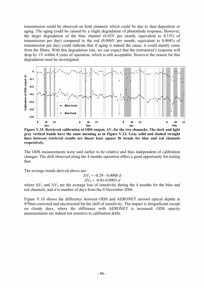
- 86 -

transmission could be observed on both channels which could be due to dust deposition or aging. The aging could be caused by a slight degradation of photodiode response. However, the larger degradation of the blue channel (0.02V per month, equivalent to 0.13% of transmission per day) compared to the red (0.006V per month, equivalent to 0.004% of transmission per day) could indicate that if aging is indeed the cause, it could mainly come from the filters. With this degradation rate, we can expect that the instrument’s response will drop by 1V within 4 years of operation, which is still acceptable. However the reason for this degradation must be investigated.

Figure V.15. Retrieved calibration of ODS output, ∆V, for the two channeks. The dark and light gray vertical bands have the same meaning as in Figure V.12. Gray solid and dashed straight lines between retrieved results are linear least square fit trends for blue and red channels respectively. The ODS measurements were said earlier to be relative and thus independent of calibration changes. The drift observed along the 4 months operation offers a good opportunity for testing that. The average trends derived above are:

∆V1 = -0.29 - 0.0008 d ∆V2 = -0.01-0.0003 d

where ∆V1 and ∆V2 are the average loss of sensitivity during the 4 months for the blue and red channels; and d is number of days from the 9 November 2004. Figure V.16 shows the difference between ODS and AERONET aerosol optical depths at 870nm corrected and uncorrected for the shift of sensitivity. The impact is insignificant except on cloudy days, where the difference with AERONET is increased. ODS opacity measurements are indeed not sensitive to calibration drifts.

- 87 -

Figure V.16. Differences between ODS and AERONET for ODS data uncorrected (boxes) and corrected (stars) for the observed shift of sensitivity the instrument.

Effect of temperature So far we have not mentioned the measurements of electronics and optical head temperatures. Figure V.17 shows the diurnal change of temperature on 23 December 2004, of 25°C amplitude. From the detector temperature dependence measured in the laboratory, the corresponding amplitude of output change will limited to 0.01V during daytime, increasing during nighttime to 0.1V because of the smaller current (10-11A) close to the dark current of photodiode. After applying the correction for temperature dependence to the ODS transfer function, the change, in opacity is only of 0.8%. The ODS measurements are little insensitive to temperature changes as those observed at Ouagadougou.

Figure V.17. Temperature of the ODS optical head and electronics on 23 December 2004. The electronics is protected inside a metallic box, thermally insulated from the outside environment, while the optical head is in direct contact with the ambient.

5.4.3 Cirrus clouds Unlike the measurement of aerosol optical depth, which is expected to be very similar to Mars, the detection of high altitude clouds is different on the Earth because of the larger density of the atmosphere and thus of the larger Rayleigh scattering. This results in a large

- 88 -

difference of altitude of the “mean scattering layer” at twilight between the blue and red photons, the first being scattered at higher altitude than the second. The presence of a thin cloud layer near the mean red scattering layer at 12-15 km at 90° SZA at twilight in the red increases the red scattered light, while the blue light scattered at higher altitude remained unchanged. The color index thus shows a bump with a maximum at a SZA highly dependent on the altitude of the cloud (Sarkissian et al. 1991). This allows detecting the presence of thin cirrus clouds in the upper troposphere and the tropopause region, hardly detectable by other techniques. As an example, Figure V.18 shows the evolution of the color index (CI) during the sunset period on 23 December 2004. A maximum reddening could be observed around 93.5° SZA and a secondary maximum around 97° SZA.

Figure V.18. ODS color index (ratio between red and blue channels) during the sunset period on 23 December 2004.

Retrieval The CI evolution at twilight has been simulated with the Monte-Carlo and SHDOM model in multiple-scattering mode in a 3D spherical atmosphere. Low altitude clouds or dust will be ignored in the following. Indeed as shown by Sarkissian et al (1991), they have little effect on the CI at twilight since they are already in the darkness. Their contribution should be limited to the attenuation of reflected light by the cirrus. The phase-function, single scattering albedo and extinction efficiency of the cloud have been calculated by the geometric-optics-integral-equation method of Yang and Liou 1996, which better applies to ice crystals than the theory of Pollack and Cuzzi originally convenient for aerosols. The cloud ice particles size distribution is assumed log-normal. From the simulations described in Chapter 4, we know that the cloud geometrical thickness has a small impact on the retrieved cloud optical depth. This parameter will be then fixed to 500 m. The cloud particle effective size and effective variance are also fixed at 4 µm and 0.25 respectively. Only cloud optical depth and cloud height are varied in the following simulations. Figure V.19 shows on the left the results of the simulation of the altitude dependence of the CI signature of a 0.08 optical thick cloud and on the right, that of the optical thickness of a cloud at 20 km, normalized in the last case at the minimum CI value after the bump. The SZA of maximum of reddening is approximately linearly dependent on the altitude of the cloud. The cloud height could be then retrieved first, independently of its optical depth, which could be derived in further step using a χ2 test. Alternatively, in a more accurate

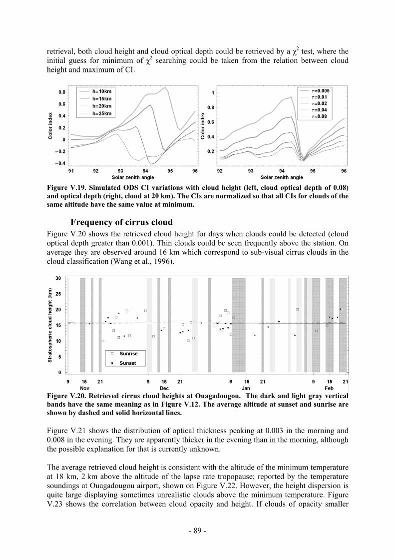
- 89 -

retrieval, both cloud height and cloud optical depth could be retrieved by a χ2 test, where the initial guess for minimum of χ2 searching could be taken from the relation between cloud height and maximum of CI.

Figure V.19. Simulated ODS CI variations with cloud height (left, cloud optical depth of 0.08) and optical depth (right, cloud at 20 km). The CIs are normalized so that all CIs for clouds of the same altitude have the same value at minimum.

Frequency of cirrus cloud Figure V.20 shows the retrieved cloud height for days when clouds could be detected (cloud optical depth greater than 0.001). Thin clouds could be seen frequently above the station. On average they are observed around 16 km which correspond to sub-visual cirrus clouds in the cloud classification (Wang et al., 1996).

Figure V.20. Retrieved cirrus cloud heights at Ouagadougou. The dark and light gray vertical bands have the same meaning as in Figure V.12. The average altitude at sunset and sunrise are shown by dashed and solid horizontal lines. Figure V.21 shows the distribution of optical thickness peaking at 0.003 in the morning and 0.008 in the evening. They are apparently thicker in the evening than in the morning, although the possible explanation for that is currently unknown. The average retrieved cloud height is consistent with the altitude of the minimum temperature at 18 km, 2 km above the altitude of the lapse rate tropopause; reported by the temperature soundings at Ouagadougou airport, shown on Figure V.22. However, the height dispersion is quite large displaying sometimes unrealistic clouds above the minimum temperature. Figure V.23 shows the correlation between cloud opacity and height. If clouds of opacity smaller

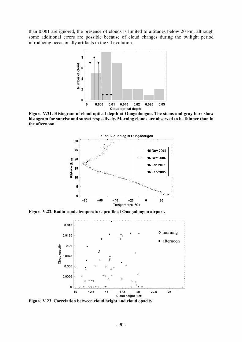
- 90 -

than 0.001 are ignored, the presence of clouds is limited to altitudes below 20 km, although some additional errors are possible because of cloud changes during the twilight period introducing occasionally artifacts in the CI evolution.

Figure V.21. Histogram of cloud optical depth at Ouagadougou. The stems and gray bars show histogram for sunrise and sunset respectively. Morning clouds are observed to be thinner than in the afternoon.

Figure V.22. Radio-sonde temperature profile at Ouagadougou airport.

Figure V.23. Correlation between cloud height and cloud opacity.

morning

afternoon

- 91 -

Other reasons for the large altitude dispersion might be the impact of low altitude dust and cloud layers (see feasibility analysis in Chapter 4), which have not been taken into account in this analysis. A more precise method for deriving the altitude of individual clouds or removing artifacts due to clouds change during the twilight period is required, which will be worked out in the future. When achieved, a correlation with temperature from daily radio-sondes should allow studying the conditions of formation of thin cirrus at the tropopause and their seasonal variation of large potential impact on climate and chemistry but difficult to observe by other methods.

5.5 Suggestions for an ODS terrestrial version The preliminary results of ODS at Ouagadougou are very encouraging. They suggest that ODS could be an efficient tool for terrestrial applications. In this last section we are proposing some modifications of ODS for improving the measurements on Earth. The suggestions include an adaptation of FOV, a change of colored filters and electronics scaling. First, since the orientation of the instrument could be controlled and the sampling frequency could be as high as desirable, a more complex FOV could be adopted, such as the one shown in Figure V.24, which would allow to increase the sampling during daytime and thus better measurements during partly cloudy days by selecting cloud free periods using the CI. A further improvement would be the use of two ODS models in parallel, the second equipped with an “inversed mask”: allowing the permanent observation of zenith scattered light and direct plus scattered light from which the optical depth could be derived even at higher sampling rate. The second suggested improvement would be to align the wavelengths of the filters on those of the AERONET photometer better adapted to the dense Earth atmosphere than those defined for the thin Mars atmosphere. For example, the red filter band could be limited to avoid the strong water vapor absorption bands around 940 nm introducing some additional noise in the current design. However, there is no need to use narrow band filters, which could create several unwanted difficulties such as temperature or aging drifts. The third recommendation would be to adjust the range of the logarithmic amplifiers so that the two channels could cover the same range and thus allow better measurements of dust optical depth from moon observations during nighttime. This would allow the investigation of a possible diurnal cycle of the dust optical depth totally unknown for the moment because no instrument until now could provide both daytime and night-time measurements. Finally, for Earth applications, the electronics need to be better protected from humidity. This modification has been already implemented recently in the model deployed at Ouagadougou.

- 92 -

Figure V.24. Proposed fields of view (FOV) for terrestrial ODS model. Left and right graphics shows “inversed field of view” of each other: when first FOV measures scattered flux, the second measures both scattered and direct flux. The white and black regions show 100% and 0% transmissions respectively. The crossing curves show an example of solar trajectories over the sky passing all masking branches.

5.6 Conclusion Four months of ODS measurements during the dry season at Ouagadougou have been analyzed showing, as expected, large increases of atmospheric opacity during Saharan dust episodes. The ODS opacities are fully consistent with that of the AERONET CIMEL photometer on clear days, but overestimated on cloudy days where the influence of dust and clouds could be hardly distinguished. A significant drift of sensitivity of the instrument was observed during the four-month operation, but which, as anticipated by the relative measurement technique adopted for the retrieval, was shown to have no impact of the precision on the measurements. Similarly, the relatively large diurnal cycle of temperature was shown to result in a very limited perturbation. Overall, the four-month validation exercise in Africa fully confirms the concept of the ODS instrument and its ability to meet with the performances required for reliable dust opacity measurements on the planet Mars. The four-month measurements available from the Ouagadougou exercise also demonstrate the ability of the system to detect ultra-thin sub-visual clouds of optical thickness as thin as 0.001 forming frequently around the cold point tropopause at the tropics. The retrieved average cloud height is consistent with the altitude of the minimum temperature although some clouds at unreasonable high altitude could be sometimes observed likely due to cloud changes during the twilight period. Although still at preliminary stage, these results are extremely encouraging. They demonstrate the feasibility of cloud height and opacity measurements with the ODS instrument in the atmosphere of Mars. But moreover, they offer a new unique method for studying the formation of ultra-thin cirrus clouds at the tropical tropopause on Earth, thought play an important role in the dehydration of the stratosphere, but almost unknown because the difficulty to observe them.

- 93 -

Chapter 6

General Conclusion A lightweight ODS (Optical Depth Sensor) instrument has been developed for daily measurements of the dust opacity of the atmosphere of Mars as well as the detection of high altitude water or CO2 ice clouds from small stations planned to be deposited on the surface of the planet during the NETLANDER mission. Though the mission is now stopped, the development has been continued up to the end of the Phase B for being ready for other potential missions. This includes a thorough simulation of the measurements, the definition and testing of the retrieval process, and finally the validation of the ODS concept and performances on the Earth by comparison with well-established systems. Dust opacity and cloud measurements in the atmosphere of Mars have been simulated by two radiative transfer models in spherical geometry. The first based on the large computation time consuming Monte-Carlo technique has been extensively tested by comparisons with analytic solutions demonstrating the model’s capability for providing accurate simulations. The second, an extension of the fast SHDOM technique to spherical geometry applications and checked against the Monte-Carlo showed remarkable performances in speed of calculation at expense of small but acceptable loss of accuracy. The two models have been used extensively to simulate the ODS observations on Mars, concluding at a high sensitivity to optical depth and high altitude clouds. A retrieval procedure for both parameters is being proposed based on the use of look-up tables and a χ2 test for determining best fitting atmospheric parameters. It has been shown that best dust opacity measurements, independent of instrument calibration drifts, aging or dust deposition at the entrance, could be obtained by fitting altogether the zenith sky intensity measurements along a full or half day. It has been demonstrated that an accuracy of a few percent could be reached on the opacity by using this technique, providing the ODS orientation is known within 0.1°. A method for deriving this orientation within the required uncertainty has been proposed based on the statistical analysis of long series of observations Sun’s pass within the field of view. Simulations also showed that clouds height and opacity could be efficiently detected by looking at the evolution of the color of the sky at twilight. A retrieval procedure based on the use of a look-up table and a χ2 optimization similar to that proposed for dust opacity has been developed with which the performances of cloud detection by the color index method has been investigated. Providing the cloud is above the dust layer (e.g. above 20 km), it was shown that its altitude could be retrieved to within ± 150m and its opacity to within 10%. Although not introduced in the retrieval process, the cloud particles effective size was also found to play a role, which is suggested to introduce in a further development. The soundness of the ODS concept, the performance of the instrument design and that of the retrieval process, have been checked by four-month observations of Saharan dust and cirrus clouds at Ouagadougou in Burkina-Faso. The optical depth measurements were found in excellent agreement with those of the well-established AERONET CIMEL photometer on clear days, but slightly overestimated on cloudy days where the influence of dust and clouds could be hardly distinguished. A significant drift of sensitivity of the instrument was observed during the four -month operation, but which, as anticipated by the relative measurement

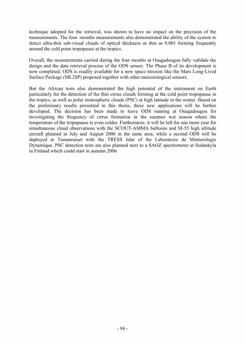
- 94 -

technique adopted for the retrieval, was shown to have no impact on the precision of the measurements. The four -months measurements also demonstrated the ability of the system to detect ultra-thin sub-visual clouds of optical thickness as thin as 0.001 forming frequently around the cold point tropopause at the tropics. Overall, the measurements carried during the four months at Ouagadougou fully validate the design and the data retrieval process of the ODS sensor. The Phase B of its development is now completed. ODS is readily available for a new space mission like the Mars Long-Lived Surface Package (ML2SP) proposed together with other meteorological sensors. But the African tests also demonstrated the high potential of the instrument on Earth particularly for the detection of the thin cirrus clouds forming at the cold point tropopause in the tropics, as well as polar stratospheric clouds (PSC) at high latitude in the winter. Based on the preliminary results presented in this thesis, these new applications will be further developed. The decision has been made to leave ODS running at Ouagadougou for investigating the frequency of cirrus formation in the summer wet season where the temperature of the tropopause is even colder. Furthermore, it will be left for one more year for simultaneous cloud observations with the SCOUT-AMMA balloons and M-55 high altitude aircraft planned in July and August 2006 in the same area, while a second ODS will be deployed at Tamanrasset with the TRESS lidar of the Laboratoire de Météorologie Dynamique. PSC detection tests are also planned next to a SAOZ spectrometer at Sodankyla in Finland which could start in autumn 2006.

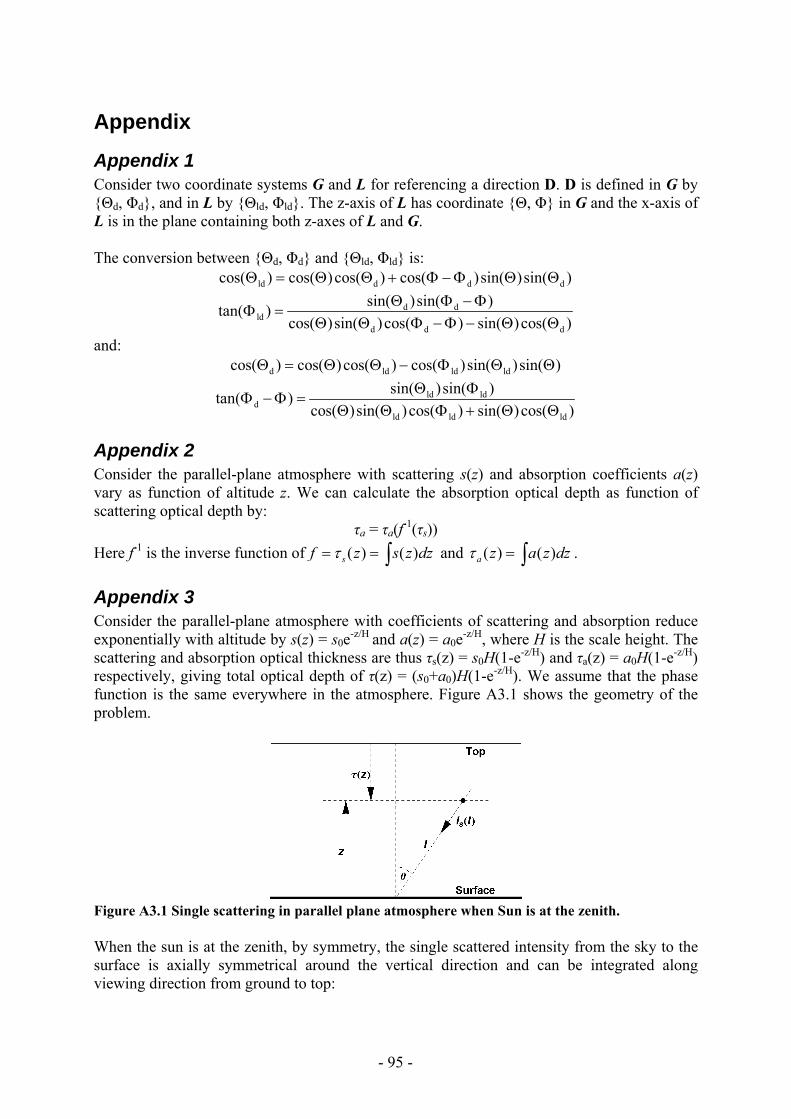
- 95 -

Appendix

Appendix 1 Consider two coordinate systems G and L for referencing a direction D. D is defined in G by {Θd, Φd}, and in L by {Θld, Φld}. The z-axis of L has coordinate {Θ, Φ} in G and the x-axis of L is in the plane containing both z-axes of L and G. The conversion between {Θd, Φd} and {Θld, Φld} is:

ld d d dcos( ) cos( )cos( ) cos( )sin( )sin( )Θ = Θ Θ + Φ −Φ Θ Θ

d dld

d d d

sin( )sin( )tan( )cos( )sin( )cos( ) sin( )cos( )

Θ Φ −ΦΦ =

Θ Θ Φ −Φ − Θ Θ

and: d ld ld ldcos( ) cos( )cos( ) cos( )sin( )sin( )Θ = Θ Θ − Φ Θ Θ

ld ldd

ld ld ld

sin( )sin( )tan( )cos( )sin( )cos( ) sin( )cos( )

Θ ΦΦ −Φ =

Θ Θ Φ + Θ Θ

Appendix 2 Consider the parallel-plane atmosphere with scattering s(z) and absorption coefficients a(z) vary as function of altitude z. We can calculate the absorption optical depth as function of scattering optical depth by:

τa = τa(f-1(τs)) Here f-1 is the inverse function of ( ) ( )sf z s z dzτ= = ∫ and ( ) ( )a z a z dzτ = ∫ .

Appendix 3 Consider the parallel-plane atmosphere with coefficients of scattering and absorption reduce exponentially with altitude by s(z) = s0e-z/H and a(z) = a0e-z/H, where H is the scale height. The scattering and absorption optical thickness are thus τs(z) = s0H(1-e-z/H) and τa(z) = a0H(1-e-z/H) respectively, giving total optical depth of τ(z) = (s0+a0)H(1-e-z/H). We assume that the phase function is the same everywhere in the atmosphere. Figure A3.1 shows the geometry of the problem.

Figure A3.1 Single scattering in parallel plane atmosphere when Sun is at the zenith.

When the sun is at the zenith, by symmetry, the single scattered intensity from the sky to the surface is axially symmetrical around the vertical direction and can be integrated along viewing direction from ground to top:

- 96 -

( )

0

( ) lsI I l e dlτ

∞−= ∫

Here µ is the cosine of zenith viewing direction (θ in Figure A3.1); l and τ(l) are the geometric and optical distance from surface, along viewing direction and Is(l) is the single scattered intensity at this distance. We have:

l = z/µ and

τ(l) = (τ – τ(z))/µ and

( )( )( ) ( )4

zs

PI z Fs z e τµ ππ

−=

Therefore: ( ) ( ( )) /

00

' ( ') /

/

( ) ( )4

( ) '4

( )1 4

z zP FI s z e e dz

P F e e d

e e P F

τ τ τ µ

τ τ τ µ

τ

τ τ µ

µ ππ µ

µ πω τπ µ

µω πµ π

∞− − −

− − −

− −

=

=

−=

−

∫

∫

Appendix 4 Consider a spherical atmosphere composed of several concentric shells where scattering coefficient can be linearly interpolated between boundaries of the shell, as shown on Figure A4.1. Within a shell with inner radius r1 and outer radius r2, we have the scattering coefficient:

s(r) = 2

2 1

r rr r−−

s1 + 1

2 1

r rr r−−

s2

Here s1 and s2 are scattering coefficient at boundaries r1 and r2.

Figure A4.1 Integration of optical depth along PQ with s(r) as linear function of radius r. Within this shell consider a photon trajectory from P to Q as shown in Figure A4.1. The geometric and optical distance between P and Q is l and τ respectively. By definition, optical depth τ is:

τ = ( )Q

P

s r d r∫ = 0

( ( ')) 'l

s r l dl∫

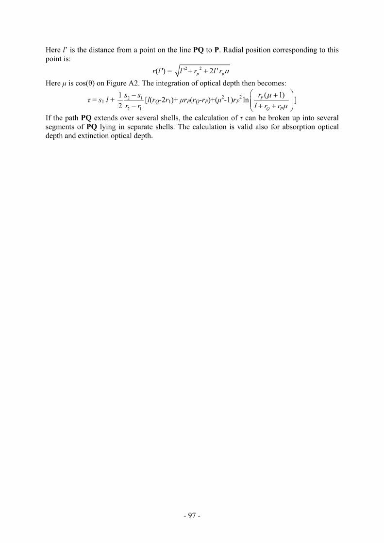
- 97 -

Here l’ is the distance from a point on the line PQ to P. Radial position corresponding to this point is:

r(l’) = 2 2' 2 'p pl r l r µ+ + Here µ is cos(θ) on Figure A2. The integration of optical depth then becomes:

τ = s1 l + 2 1

2 1

12

s sr r−−

[l(rQ-2r1)+ µrP(rQ-rP)+(µ2-1)rP2 ( 1)ln P

Q P

rl r r

µµ

⎛ ⎞+⎜ ⎟⎜ ⎟+ +⎝ ⎠

]

If the path PQ extends over several shells, the calculation of τ can be broken up into several segments of PQ lying in separate shells. The calculation is valid also for absorption optical depth and extinction optical depth.

- 98 -

References

Anderson E. and Leovy C., Mariner 9 Television Limb Observations of Dust and Ice Hazes on Mars, Journal of the Atmospheric Sciences, 35 (4), 723–734, 1977.

Arfken G., Mathematical Methods for Physicists, 4th ed. Academic Press, 739-740, 1995.

Barret, B., De Maziere, M., Demoulin, P., Retrieval and characterization of ozone profiles from solar infrared spectra at the Jungfraujoch, J. Geophys. Res., 107 (D24), 4788, 2002.

Bell III, J.F., Calvin, W.M., Ockert-Bell, M.E. et al. Detection and monitoring of H2O and CO2 ice clouds on Mars, J. Geophys. Res., 101, 9227-9238, 1996.

Bucholtz A., Rayleigh-scattering calculations for the terrestrial atmosphere, Applied Optics, 34 (15), 2765-2773, 1995.

Cattrall and Carder, Columnar aerosol single-scattering albedo and phase function retrieved from sky radiance over the ocean: Measurements of Saharan dust, J. Geophys. Res., 108 (D9), 4287, 2003.

Chandrasekhar, S., Radiative Transfer, Dover, New York, 1960.

Clancy, R. T., M. J. Wolff, and P. R. Christensen, Mars aerosol studies with the MGS TES emission phase function observations: Optical depths, particle sizes, and ice cloud types versus latitude and solar longitude, J. Geophys. Res., 108 (E9), 5098, 2003.

Clancy, R.T., Grossman, A.W., Wolff, M. J. et al. Water vapor saturation at low altitudes around Mars aphelion: A key to Mars climate?, Icarus, 122, 36-62, 1996.

Colarco, P. R. and Toon, O. B., Determining the UV imaginary index of refraction of Saharan dust particles from Total Ozone Mapping Spectrometer data using a three-dimensional model of dust transport, J. Geophys. Res., 107 (D16), AAC 4-1, 2002.

Colburn, D. S. Pollack, J. B. and Haberle, R. M. Diurnal variations in optical depth at Mars, Icarus, 79, 159-189, 1989.

Collins, M., Lewis, S.R., Read, P.L. et al. A climate database for the Martian atmosphere, in Environment Modeling for Space-based Applications, European Space Agency SP-392, 323-327, 1996.

Diu, B., Guthmann, C., Lederer, D., and Roulet., B., Elements de Physique Statistique, Hermann, Paris, 1989.

Dubovik et al., Variability of Absorption and Optical Properties of Key Aerosol Types Observed in Worldwide Locations, J. Atmos. Sci., 59, 590, 2001.

Dubovik, O., Holben, B. N., Lapyonok, T., et al., Non-spherical aerosol retrieval method employing light scattering by spheroids, Geophys. Res. Lett., 29 (10), 54-1, 2002.

Evans, K. F., The Spherical Harmonics Discrete Ordinate Method for Three-Dimensional Atmospheric Radiative Transfer, Journal of the Atmospheric Science, 55, 429-446, 1998.

Gerstl, S. A. W., and A. Zardecki, Discrete-ordinates finite element method for atmospheric radiative transfer and remote sensing. Appl. Opt., 24, 81–93, 1985.

Gierasch, P. J. and Goody, R. M. The effect of dust on the temperature of the Martian atmosphere, J. Atmos. Sci., 29, 400-402, 1972.

- 99 -

Gill, P. R., Murray, W., and Wright, M. H. The Levenberg-Marquardt Method §4.7.3 in Practical Optimization, London, Academic Press, 136-137, 1981.

Gooding, J. L., Martian dust as condensation nuclei: A preliminary assessment of mineralogical factors, Icarus, 66, 55-74, 1986.

Haberle, R. M., et al. Some effect of global dust storms on the atmospheric circulation of Mars, Icarus, 50, 322-367, 1982.

Haberle, R. M. and Jakosky, B. M. Sublimation and transport of water from the North residual polar cap on Mars, J. Geophys. Res., 95, 1423-1437, 1990.

Haberle, R. M., Catling, D. C., Chassefiere, E., et al., The Pascal Discovery Mission: A Mars Climate Network Mission, Concepts and Approaches for Mars Exploration, 135, 2000.

Harri, A-M., Linkin, V., Polkko, J., et al. Meteorological observations on Martian surface : met-packages of Mars-96 small stations and penetrators, Planet. Space. Sci., 46, 779-793, 1998.

Haywood, J., Francis, P., Osborne, S., et al., Radiative properties and direct radiative effect of Saharan dust measured by the C-130 aircraft during SHADE:1. Solar spectrum, J. Geophys. Res., 108 (D18), 8577, 2003.

Hedin, A. E., Extension of the MSIS Thermospheric Model into the Middle and Lower Atmosphere, J. Geophys. Res., 96, 1159, 1991.

Henyey, L.G. and Greenstein J.L., Diffuse radiation in the galaxy, Astrophysical Journal, 93, 70-83, 1941.

Highwood, E. J., Haywood, J. M., Silverstone, M., et al., Radiative properties and direct effect of Saharan dust measured by the C-130 aircraft during Saharan Dust Experiment (SHADE). 2: Terrestrial spectrum, J. Geophys. Res., 108 (D18), 8578, 2003.

Hoffman, P. The Man Who Loved Only Numbers: The Story of Paul Erdos and the Search for Mathematical Truth. New York: Hyperion, pp. 238-239, 1998.

Hsu, N.C., et al. Comparison of the TOMS Aerosol Index with Sunphotometer Aerosol Optical Thickness: Results and Applications, J. Geophys. Res., 104, 6269-6279, 1999.

Hu Y.X. et al., Delta-Fit: A fast and accurate treatment of particle scattering phase functions with weighted singular-value decomposition least-squares fitting, Journal of Quantitative Spectroscopy & Radiative Transfer, 65, 681-690, 2000

James, P. B. The role of water ice clouds in the Martian hydrological cycle, J. Geophys. Res., 95, 1439-1445, 1990.

Joseph, J. H., Wiscombe, W. J., Weinman, J. A., The delta-Eddington approximation for radiative flux transfer, Journal of the Atmospheric Sciences, 33, 2452-2459, 1976.

Krasnopolsky, V. A., J. P. Maillard, T. C. Owen, Detection of methane in the Martian atmosphere: evidence for life?, Icarus, 172 (2), 537-547.

Kuo, K.-S., R. C. Weger, R. M. Welch, and S. K. Cox, The Picard iterative approximation to the solution of the integral equation of radiative transfer. Part II: Three-dimensional geometry, J. Quant. Spectrosc. Radiat. Transfer, 55, 195–213, 1996.

Landis, G. and Jenkins, P. Measurement of the Settling Rate of Atmospheric Dust on Mars by the MAE Instrument on Mars Pathfinder, J. Geophys. Res., 105, 1855-1857, 2000.

Lenoble, J., Atmospheric Radiative Transfer, Hampton, Virginia: Deepak Publishing, 1993.

- 100 -

Léon, J. F., Tandré D., Pelon J., et al., Profiling of a Saharan dust outbreak based on a synergy between active and passive remote sensing, J. Geophys. Res., 108 (D18), 8575, 2003.

Likin, V., et al., Harri, A.-M., Lipatov, A., et al., A sophisticated lander for scientific exploration of Mars: scientific objectives and implementation of the Mars-96 Small Station, Planetary and Space Science, 46, 717-737, 1998.

Marchuk, G., G. Mikhailov, M. Nazaraliev, R. Darbinjan, B. Kargin, and B. Elepov, The Monte Carlo Methods in Atmospheric Optics, Springer-Verlag, 208 pp, 1980.

Maria, J.-L., Tran, T.T., Pommereau, J. P. et al., Technical aspect of Optical Depth Sensor, Advances in Space Research, accepted.

Markiewicz, W.J., Sablotny, R.M., Keller, H.U., et al., Optical properties of the Martian aerosols as derived from Imager for Mars Pathfinder midday sky brightness data, J. Geophys. Res., 104, 9009-9017, 1999.

Marsal, O., Venet, M., Counil, J-L., Ferri, F., Harri, A-M., Spohn, T., Block, J., The NetLander geophysical network on the surface of Mars: General mission description and technical design status, Acta Astronautica, 51 (1-9), 379-386, 2002.

Meador, W.E. and Weaver, W.R, Two-Stream Approximations to Radiative Transfer in Planetary Atmospheres: A Unified Description of Existing Methods and a New Improvement, Journal of the Atmospheric Sciences, 37, 630-643, 1980.

Metropolis, N. and Ulam, S., 1949, The Monte Carlo Method, J. Amer. Stat. Assoc., 44, 335-341.

Metropolis, N., 1987, The Beginning of the Monte Carlo Method, Los Alamos Science, No. 15, p. 125. http://jackman.stanford.edu/mcmc/metropolis1.pdf.

Montmessin, F., Rannou, P., Cabane, M., New insights into Martian dust distribution and water-ice cloud microphysics, Journal of Geophysical Research, 102, 10997-11013, 2002

Myhr, G., Grini, Al., Haywood, J. M., et al., Modeling the radiative impact of mineral dust during the Saharan Dust Experiment (SHADE) campaign, J. Geophys. Res., 108 (D18), 8579, 2003.

O’Brien, D. M., Accelerated quasi Monte Carlo integration of the radiative-transfer equation, J. Quant. Spectrosc. Radiat. Transfer, 48, 41–59, 1992.

Ockert-Bell, M.E., Bell III, J.F., Pollack, J.P. et al., Absorption and scattering properties of the Martian dust in the solar wavelength, J. Geophys. Res., 102, 9039-9050, 1997.

Pollack J.B. and J.N. Cuzzi, Scattering by non-spherical particles of sizes comparable to wavelength – A new semi-emperical theory and its application to tropospheric aerosols, Journal of Atmospheric Science, 37, 868-881, 1980.

Pommereau, J. P. and F. Goutail, O3 and NO2 ground-based measurement by visible spectrometry during artic winter and spring 1988, Geophy. Res. L., 15, 891-94, 1988.

Randall, C. E., Lumpe, J. D., Bevilacqua, R. M., et al., Dynamical properties of Mars water ice clouds and their interaction with atmospheric dust and radiation, Adv. Space Res., 23, 9, 1577-1585, 1999.

Salinas, S.V., Grieger, B., Rodin, A.V., Keller, H.U., 2003, A spherical model for computing polarized radiation in Titan’s atmosphere, Planetary and Space Science, 51, 977-989.

Sarkissian, A., Pommereau, J. P. and Goutail, F., Identification of polar stratospheric clouds from the ground by visible spectrometry, Geophys. Res. Lett., 18 (4), 779-782, 1991.

- 101 -

Sarkissian, A., Pommereau, J. P., Goutail, F., et al., PSC and volcanic aerosol observations during EASOE by UV-visible ground-based spectrometry, Geophys. Res. Lett., 21, 1319-1322, 1994.

Schneider, W., Moorgat, G. K., Tyndall, G. S., et al., Absorption crossections of NO2 in the UV and visible regions (200 - 700nm) at 289 K., J. Photochem. Photobiol, 40, 195-217, 1987.

Sinyuk, A., Torres, O., and Dubovik, O., Combined use of satellite and surface observations to infer the imaginary part of refractive index of Saharan dust, Geophys. Res. Lett., 30 (2), 1081, 2003.

Smith, M.D., et al., One Martian year of atmospheric observations by the Thermal Emission Spectrometer, Geophys. Res. Lett., 28 (22), 4263-4266, 2001.

Stenholm, L. G., H. Storzer, and R.Wehrse, An efficient method for the solution of 3D radiative transfer problems, J. Quant. Spectrosc. Radiat. Transfer, 45, 47–56, 1991.

Tanré, D., et al., Measurement and modeling of the Saharan dust radiative impact: Overview of the Saharan Dust Experiment (SHADE), J. Geophys. Res., 108, 8574, 2003.

Toon, O.B., McKay, C.P., Ackerman, T.P., and Santhanam, K., 1989, Rapid Calculation of Radiative Heating Rates and Photodissociation Rates in Inhomogeneous Multiple Scattering Atmospheres, Journal of Geophysical Research, 94, 16287-16301.

Tran, T. T. and Rannou, P. Comparing 3D spherical Monte-Carlo and 2-stream parallel plane simulation of far-field backscattering image of Titan, http://www.ipsl.jussieu.fr/documentation/NotesPlaneto/Archives/NPP_2.pdf, 2004.

Tran, T. T., Pommereau, J. P., Rannou, P., et al., Scientific aspect of Optical Depth Sensor, Advances in Space Research, 36, 2182–2186, 2005.

van der A, R. J., van Oss, R. F., Piters, A. J. M., et al., Ozone profile retrieval from recalibrated Global Ozone Monitoring Experiment data, J. Geophys. Res., 107 (D15), 4239, 2002.

van de Hulst, H. C., Light scattering by small particles, New York, Dover, 1981.

Volten et al., Scattering matrices of mineral aerosol particles at 441.6 nm and 632.8 nm, J. Geophys. Res., 15, 17375-17401, 2001.

Wallace, Alfred Russel, Is Mars habitable? A critical examination of Professor Percival Lowell's book "Mars and its canals," with an alternative explanation, by Alfred Russel Wallace, F.R.S., etc. London, Macmillan and co., 1907.

Wang, J., Christopher, S. A., Reid, J. S., et al., GOES 8 retrieval of dust aerosol optical thickness over the Atlantic Ocean during PRIDE, J. Geophys. Res., 108 (D19), 8595, 2003.

Wang, P.-H., Minnis, P., McCormick, M. P. et al, A 6-year climatology of cloud occurrence frequency from Stratospheric Aerosol and Gas Experiment II observations (1985-1990), Journal of Geophysical Research, 101 (D23), 29407-29430, 1996.

Warren, S. G., Optical constants of ice from the ultraviolet to the microwave, Appl. Optics., 23, 1206–1225, 1984.

Wiscombe, W. J., The Delta-M Method: Rapid Yet Accurate Radiative Flux Calculations for Strongly Asymmetric Phase Functions, Journal of Atmospheric Sciences, 34 (9), 1408-1422, 1977.

Wolff, M. J., and R. T. Clancy, Constraints on the size of Martian aerosols from Thermal Emission Spectrometer observations, J. Geophys. Res., 108 (E9), 5097, 2003.

- 102 -

Yang, P., and Liou, K. N., Geometric-optics-integral-equation method for light scattering by nonspherical ice crystal, Applied Optics, 35 (33), 6568-6584, 1996.