Dissertation submitted to the Combined Faculties of the Natural Sciences and Mathematics of the Ruperto-Carola-University of Heidelberg, Germany for the degree of Doctor of Natural Sciences Put forward by Hendrik Bekker MSc. born in: Groningen, the Netherlands Oral examination: 18-05-2016

Welcome message from author
This document is posted to help you gain knowledge. Please leave a comment to let me know what you think about it! Share it to your friends and learn new things together.
Transcript

Dissertationsubmitted to the
Combined Faculties of the Natural Sciences and Mathematicsof the Ruperto-Carola-University of Heidelberg, Germany
for the degree ofDoctor of Natural Sciences
Put forward by
Hendrik Bekker MSc.
born in: Groningen, the Netherlands
Oral examination: 18-05-2016


Optical and EUV spectroscopy of highlycharged ions near the 4 f –5s level
crossing
Referees: PD Dr. José R. Crespo López-Urrutia
PD Dr. Wolfgang Quint

Optical and EUV spectroscopy of highly charged ions near the 4 f –5s
level crossing
In recent years, various highly charged ions (HCI) with optical transitions have been proposedfor metrology and searches of a possible variation of the fine-structure constant α . Opticaltransitions in HCI are uncommon due to the scaling of energy levels with atomic numberZ2. At the 4 f –5s level crossing, three configurations are nearly degenerate, and thus manyoptical transitions can exist. The complex many-electron couplings reduce the accuracy ofcurrent calculations. Moreover, experimental data to benchmark the predictions is lacking.Spectra in the optical and extreme-ultraviolet (EUV) range of several ion species near the4 f –5s level crossing were measured at the Heidelberg electron beam ion trap. A collisional-radiative model was employed for the interpretation of the EUV data, resulting in the firstidentification of the long sought-after 5s–5p transitions in Pm-like Re14+, Os15+, Ir16+, andPt17+. The characteristic line shapes of optical transitions in Ir17+ were studied, with theaim of identifying transitions with a high sensitivity to α-variation. Previously suggestedcandidates could be excluded and new candidates were proposed. This data provides astringent benchmark for state-of-the-art precision atomic theory.
Optische und EUV Spektroskopie hochgeladener Ionen in der Umge-bung der 4 f –5s-Niveaukreuzung
In den letzten Jahren wurden verschiedene hochgeladene Ionen (HCI) mit optischen Übergän-gen sowohl für die Metrologie als auch für die Suche nach einer möglichen Zeitabhängigkeitder Feinstrukturkonstanten α vorgeschlagen. Solche Übergänge treten wegen der Skalierungder Energienniveaus mit der Atomzahl Z2 bei HCI selten auf. Jedoch sind bei der 4 f –5sKreuzung drei unterschiedliche elektronische Konfigurationen energetisch nahezu entartet,wodurch eine Vielzahl optischer Übergänge zwischen ihnen stattfinden kann. Die komplexenKopplungen der Elektronen vermindern die Genauigkeit aktueller Stukturrechnungen. Zu-dem existieren kaum experimentelle Daten, um jene zu überprüfen. Es wurden Spektrensowohl im optischen als auch im extremen-ultravioletten (EUV) Bereich mittels der Hei-delberger Electron Beam Ion Trap aufgenommen. Mit Hilfe eines kollisionellen-radiativenModells wurden die EUV-Daten analysiert, wobei die erste Identifizierung der langgesuchtenÜbergänge 5s–5p in Pm-artigen Re14+, Os15+, Ir16+ und Pt17+ gelang. Die charakter-istischen Linienprofile der optischen Übergänge in Ir17+ wurden zur Identifizierung vonLinien mit hoher Empfindlichkeit für eine α-Variation untersucht. Es konnten dabei frühereVorschläge ausgeschlossen und neue Kandidaten ausgemacht werden. Die gewonnenenDaten stellen akkurate Prüfsteine für moderne Präzisionsrechnungen der Atomtheorie dar.


Table of contents
Abstract v
1 Introduction and motivation 11.1 Searches for variation of fundamental constants . . . . . . . . . . . . . . . 21.2 Highly charged ions as frequency standards . . . . . . . . . . . . . . . . . 51.3 Ir17+ as a highly sensitive detector of variation of the fine-structure constant 81.4 Alkali-like systems near the 4 f –5s level crossing . . . . . . . . . . . . . . 10
2 Theory 132.1 Basics of Atomic Physics . . . . . . . . . . . . . . . . . . . . . . . . . . . 13
2.1.1 Hydrogen-like systems . . . . . . . . . . . . . . . . . . . . . . . . 142.1.2 Many-electron systems . . . . . . . . . . . . . . . . . . . . . . . . 152.1.3 The Wigner-Eckart theorem . . . . . . . . . . . . . . . . . . . . . 172.1.4 Zeeman splitting . . . . . . . . . . . . . . . . . . . . . . . . . . . 172.1.5 Zeeman transitions . . . . . . . . . . . . . . . . . . . . . . . . . . 18
2.2 Electron-ion interactions in an EBIT . . . . . . . . . . . . . . . . . . . . . 222.3 Computational methods in atomic physics . . . . . . . . . . . . . . . . . . 24
2.3.1 The configuration interaction method . . . . . . . . . . . . . . . . 252.3.2 The coupled cluster method . . . . . . . . . . . . . . . . . . . . . 262.3.3 The collisional radiative model . . . . . . . . . . . . . . . . . . . . 27
3 Experimental setup 293.1 The electron beam ion trap . . . . . . . . . . . . . . . . . . . . . . . . . . 30
3.1.1 The electron gun . . . . . . . . . . . . . . . . . . . . . . . . . . . 313.1.2 The central region . . . . . . . . . . . . . . . . . . . . . . . . . . 343.1.3 The trap and the electron beam . . . . . . . . . . . . . . . . . . . . 343.1.4 The electron collector . . . . . . . . . . . . . . . . . . . . . . . . 373.1.5 The injection system . . . . . . . . . . . . . . . . . . . . . . . . . 38

Table of contents
3.2 Spectroscopic instrumentation . . . . . . . . . . . . . . . . . . . . . . . . 39
3.2.1 Blazed diffraction gratings . . . . . . . . . . . . . . . . . . . . . . 40
3.2.2 CCD cameras . . . . . . . . . . . . . . . . . . . . . . . . . . . . . 41
4 Spectroscopy of Pm-like and Nd-like systems in the extreme ultra-violet regime 434.1 Vacuum ultra-violet spectrometer . . . . . . . . . . . . . . . . . . . . . . . 45
4.2 Calibration . . . . . . . . . . . . . . . . . . . . . . . . . . . . . . . . . . 48
4.3 Data analysis . . . . . . . . . . . . . . . . . . . . . . . . . . . . . . . . . 49
4.4 EUV spectra of Re, Os, Ir, and Pt . . . . . . . . . . . . . . . . . . . . . . . 53
4.4.1 Full overview of the acquired data . . . . . . . . . . . . . . . . . . 53
4.4.2 Charge state determination . . . . . . . . . . . . . . . . . . . . . . 55
4.5 Identifications of lines in the Pm-like spectra . . . . . . . . . . . . . . . . . 57
4.5.1 Influence of the electron beam density . . . . . . . . . . . . . . . . 58
4.5.2 Comparison of the 5s - 5p wavelengths to predictions . . . . . . . . 61
4.6 Identifications of transitions in the Ir17+ spectrum . . . . . . . . . . . . . . 62
5 Spectroscopy in the optical regime 715.1 The optical spectrometer setup . . . . . . . . . . . . . . . . . . . . . . . . 71
5.2 Measurement procedure . . . . . . . . . . . . . . . . . . . . . . . . . . . . 74
5.3 Analysis procedure . . . . . . . . . . . . . . . . . . . . . . . . . . . . . . 77
5.3.1 Removal of cosmics . . . . . . . . . . . . . . . . . . . . . . . . . 77
5.3.2 Image correction and row selection . . . . . . . . . . . . . . . . . 79
5.3.3 Composing the final spectrum . . . . . . . . . . . . . . . . . . . . 81
5.3.4 Fitting of lines with Zeeman components . . . . . . . . . . . . . . 83
6 Measurement and interpretation of the optical spectra 876.1 Overview of precision spectra . . . . . . . . . . . . . . . . . . . . . . . . 88
6.2 Identification of missing M1 lines . . . . . . . . . . . . . . . . . . . . . . 95
6.2.1 Identification of the 1Fo3 –3Fo
3 transition . . . . . . . . . . . . . . . 95
6.2.2 Identification of the 3P2 - 1D2 transition . . . . . . . . . . . . . . . 96
6.2.3 Identification of the 3H4–3F3 transition . . . . . . . . . . . . . . . 97
6.3 Search for interconfiguration E1 lines . . . . . . . . . . . . . . . . . . . . 99
6.3.1 Exclusion of E2 transitions . . . . . . . . . . . . . . . . . . . . . . 100
6.3.2 Ryberg-Ritz principle for E1 lines . . . . . . . . . . . . . . . . . . 100
6.4 Zeeman fits of the E1 candidates . . . . . . . . . . . . . . . . . . . . . . . 104
6.5 CRM predictions . . . . . . . . . . . . . . . . . . . . . . . . . . . . . . . 109
viii

Table of contents
7 Summary and outlook 111
Acknowledgements 117
References 119
Appendix A Predicted E1 line shapes 131
Appendix B FAC and CRM example scripts 135B.1 Calculation of energy levels, tranition rates, and excitation cross-sections . . 135B.2 Collisional radiative model . . . . . . . . . . . . . . . . . . . . . . . . . . 137B.3 Generation of a synthetic spectrum . . . . . . . . . . . . . . . . . . . . . . 138
Appendix C EUV lines of Nd-like and Pr-like Re, Os, Ir, and Pt 139
ix

Chapter 1
Introduction and motivation
Ceaseless change is the only constant thing in nature.
John Candee Dean [1]
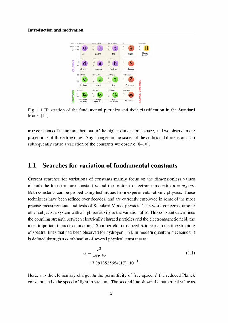
Since the dawn of our existence humankind has developed increasingly intricate modelsto understand, explain, and control nature. And yet, with every advancement in our un-derstanding, new questions arise. At the forefront of our current understanding of particlephysics is the Standard Model. It describes the properties and the possible interactions of17 fundamental particles, refer to Fig. 1.1 for a schematic overview. Over the years, minoradjustments had to be made to the Standard Model, most prominently the addition of theHiggs boson [2, 3]. Nonetheless, the Standard Model has proven to be highly successfulat predicting and describing nature [4]. Despite these successes, there are questions thatthe Standard Model provokes. One of these questions has to do with the way fundamentalparticles interact with each other. Mathematically this is fully described in the StandardModel. Determining for the actual strengths of the interactions are the coupling constants.These, together with the masses of the fundamental particles, form approximately 20 freeparameters of the Standard Model. Their actual values have been found by measurements.However, one can ask: why do they have the values they have? Could these be predictedfrom first principles? And also, are the constants truly constant in time? After all, if there isanything that our observations of the universe have taught us, it is that change is ceaseless.
The possibility of varying constants was already considered by notable physicists such asDirac, Teller, and Gamow [5–7]. The original idea of Dirac that the gravitational constantvaries with time was disproved by Teller and Gamov. However, the latter suggested that thefine-structure constant could vary with time. Till this day, the possible variation of constantsremains a widely discussed topic in physics. For example, many current theories beyond theStandard Model introduce extra spatial dimensions in addition to the three familiar ones. The
1
Introduction and motivation
Fig. 1.1 Illustration of the fundamental particles and their classification in the StandardModel [11].
true constants of nature are then part of the higher dimensional space, and we observe mereprojections of those true ones. Any changes in the scales of the additional dimensions cansubsequently cause a variation of the constants we observe [8–10].
1.1 Searches for variation of fundamental constants
Current searches for variations of constants mainly focus on the dimensionless valuesof both the fine-structure constant α and the proton-to-electron mass ratio µ = mp/me.Both constants can be probed using techniques from experimental atomic physics. Thesetechniques have been refined over decades, and are currently employed in some of the mostprecise measurements and tests of Standard Model physics. This work concerns, amongother subjects, a system with a high sensitivity to the variation of α . This constant determinesthe coupling strength between electrically charged particles and the electromagnetic field, themost important interaction in atoms. Sommerfeld introduced α to explain the fine structureof spectral lines that had been observed for hydrogen [12]. In modern quantum mechanics, itis defined through a combination of several physical constants as
α =e2
4πε0hc(1.1)
= 7.2973525664(17) ·10−3.
Here, e is the elementary charge, ε0 the permittivity of free space, h the reduced Planckconstant, and c the speed of light in vacuum. The second line shows the numerical value as
2
1.1 Searches for variation of fundamental constants
recommended by CODATA [13]. Two methods to determine the variation of α are discussednext.
The first method exploits techniques and advances from the science of measurement, i.e.metrology. Current state of the art frequency standards developed at metrology institutes suchas NIST1, NPL2, and the PTB3 reach extremely small fractional uncertainties, the currentrecord being at the level of 10−18 [14–16]. The unprecedented precision achieved by thesecan be used to determine upper limits for the variations of α and µ . In a modern frequencystandard (clock), a laser is locked to an optical transition of an ion. Simultaneously, thefrequency ν of the laser light can be compared to another clock, for example by means of afrequency comb. Assuming the transition energy of the ion does not change over time, thelaser frequency will not change. However, the transition energy of the ion depends on thevalue of the fine-structure constant. Thus if α changes, the initial clock frequency at time tiwill have shifted to
ν(t f ) = ν(ti)+2q1α
dα
dt(1.2)
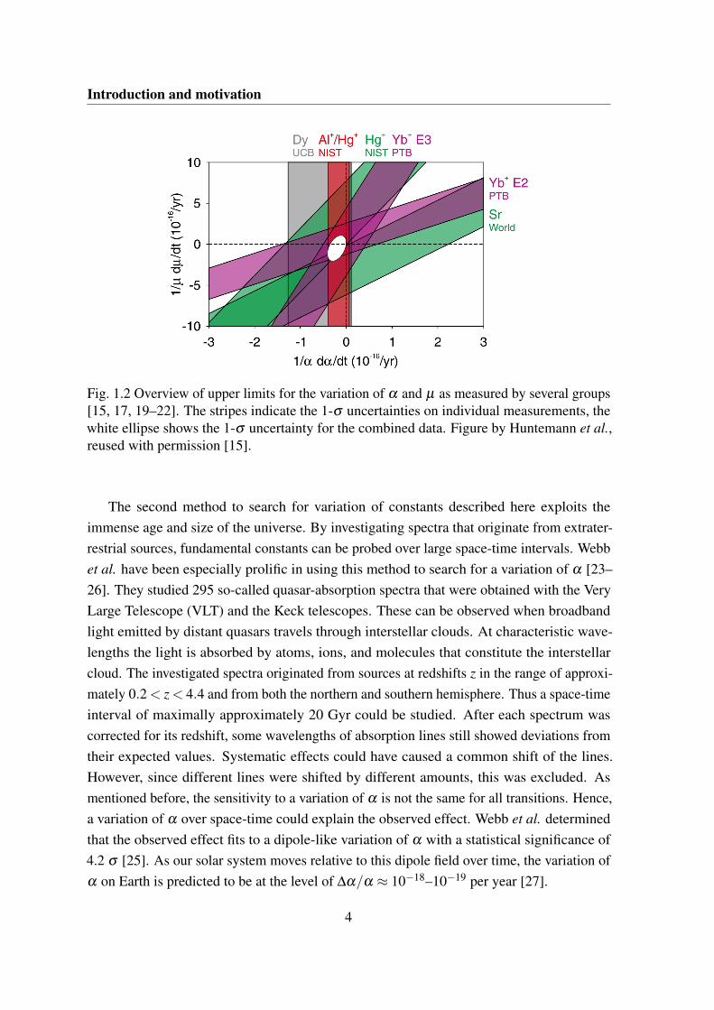
at time t f . The sensitivity factor q is introduced here to parametrize the sensitivity to thevariation of α . By comparing two clocks with different sensitivity factors to each other whiletime evolves, it is possible to determine the variation of α . The most successful measurementof this kind was performed by comparing a transition of Al+ with a transition of Hg+ severaltimes over the course of approximately a year [17]. In this case, the q factor of the Al+
transition is essentially zero, while the q factor of the Hg+ transition is approximately-52 200 cm−1 [18]. An overview of results obtained by experiments around the worldis shown in Fig. 1.2. The simultaneous sensitivity to the variation of µ of some of themeasurements is due to comparisons with hyperfine transitions. The transition energies ofthese directly depend on the proton-to-electron mass ratio. By combining the data sets, thecurrently most stringent limits to the variations were determined to be [15]
1α
dα
dt=−2.0(2.0) ·10−17/yr (1.3)
1µ
µ
dt= 5(16) ·10−17/yr. (1.4)
Thus, at the current level of precision, the results are consistent with no variation.
1National Institute of Standards and Technology, United States2National Physical Laboratory, United Kingdom3Physikalisch-Technische Bundesanstalt, Germany
3
Introduction and motivation
Fig. 1.2 Overview of upper limits for the variation of α and µ as measured by several groups[15, 17, 19–22]. The stripes indicate the 1-σ uncertainties on individual measurements, thewhite ellipse shows the 1-σ uncertainty for the combined data. Figure by Huntemann et al.,reused with permission [15].
The second method to search for variation of constants described here exploits theimmense age and size of the universe. By investigating spectra that originate from extrater-restrial sources, fundamental constants can be probed over large space-time intervals. Webbet al. have been especially prolific in using this method to search for a variation of α [23–26]. They studied 295 so-called quasar-absorption spectra that were obtained with the VeryLarge Telescope (VLT) and the Keck telescopes. These can be observed when broadbandlight emitted by distant quasars travels through interstellar clouds. At characteristic wave-lengths the light is absorbed by atoms, ions, and molecules that constitute the interstellarcloud. The investigated spectra originated from sources at redshifts z in the range of approxi-mately 0.2 < z < 4.4 and from both the northern and southern hemisphere. Thus a space-timeinterval of maximally approximately 20 Gyr could be studied. After each spectrum wascorrected for its redshift, some wavelengths of absorption lines still showed deviations fromtheir expected values. Systematic effects could have caused a common shift of the lines.However, since different lines were shifted by different amounts, this was excluded. Asmentioned before, the sensitivity to a variation of α is not the same for all transitions. Hence,a variation of α over space-time could explain the observed effect. Webb et al. determinedthat the observed effect fits to a dipole-like variation of α with a statistical significance of4.2 σ [25]. As our solar system moves relative to this dipole field over time, the variation ofα on Earth is predicted to be at the level of ∆α/α ≈ 10−18–10−19 per year [27].
4
1.2 Highly charged ions as frequency standards
Due to the complexity associated with the interpretation of the quasar-absorption spectra,the results are controversial. Webb et al. themselves indicate that although significantefforts were made to exclude systematic effects, more measurements with other telescopesare required to constrain systematic effects further [25]. Moreover, Whitmore and Murphypointed out systematic errors of the wavelength scales of the employed spectrometers at theVLT and Keck telescopes [28]. Currently, new measurements of quasar-absorption spectraspecifically aimed at the search for α variation are being performed. Recently, an analysisincluding some of the new data was published [29]. The results support the dipole model.However, the amplitude of the dipole was found to be slightly smaller. When variation of afundamental constant is claimed, compelling evidence from multiple sources is required tomake such a profound statement plausible. Several other methods to search for variation ofthe fine-structure constant and other constants have been proposed and applied. An overviewof such searches can be found for example in the work by Uzan [30]. The aforementionedmethod based on frequency standards has the advantage that the experimental parameters arepotential well under control.
1.2 Highly charged ions as frequency standards
Currently, the second is defined as “9 192 631 770 periods of the radiation correspondingto the transition between the two hyperfine levels of the ground state of the caesium 133atom” [31]. Proposed novel frequency standards use transitions with much shorter periods.Now, the radiation is in the optical regime, instead of the microwave regime of the cesiumtransition. This makes the fractional uncertainty
σ =∆ν
ν0(1.5)
much smaller. Assuming identical frequency uncertainties ∆ν , the fractional uncertainty foran optical transition centered at a frequency ν0 can theoretically be a factor of 105 smaller[32]. This level of improvement has not yet been achieved due to the challenges associatedwith reducing ∆ν . The precision with which optical frequencies can be measurement hasdramatically improved over the last decades, among others, due to the development offemtosecond frequency combs [33]. Additionally, by choosing transitions with line widthsof 1 Hz or less, the central frequency ν0 can be determined with extremely high precision.However, the uncertainty is not only due to statistical errors, but also due to uncertaintiesthat systematic effects introduce [16].
5
Introduction and motivation
7 4 7 5 7 6 7 7 7 8
0
1 0
2 0
3 0
4 0
4 f 1 2 5 s 2
4 f 1 3 5 s 1
Ene
rgy
(eV
)
A t o m i c n u m b e r Z
4 f 1 4
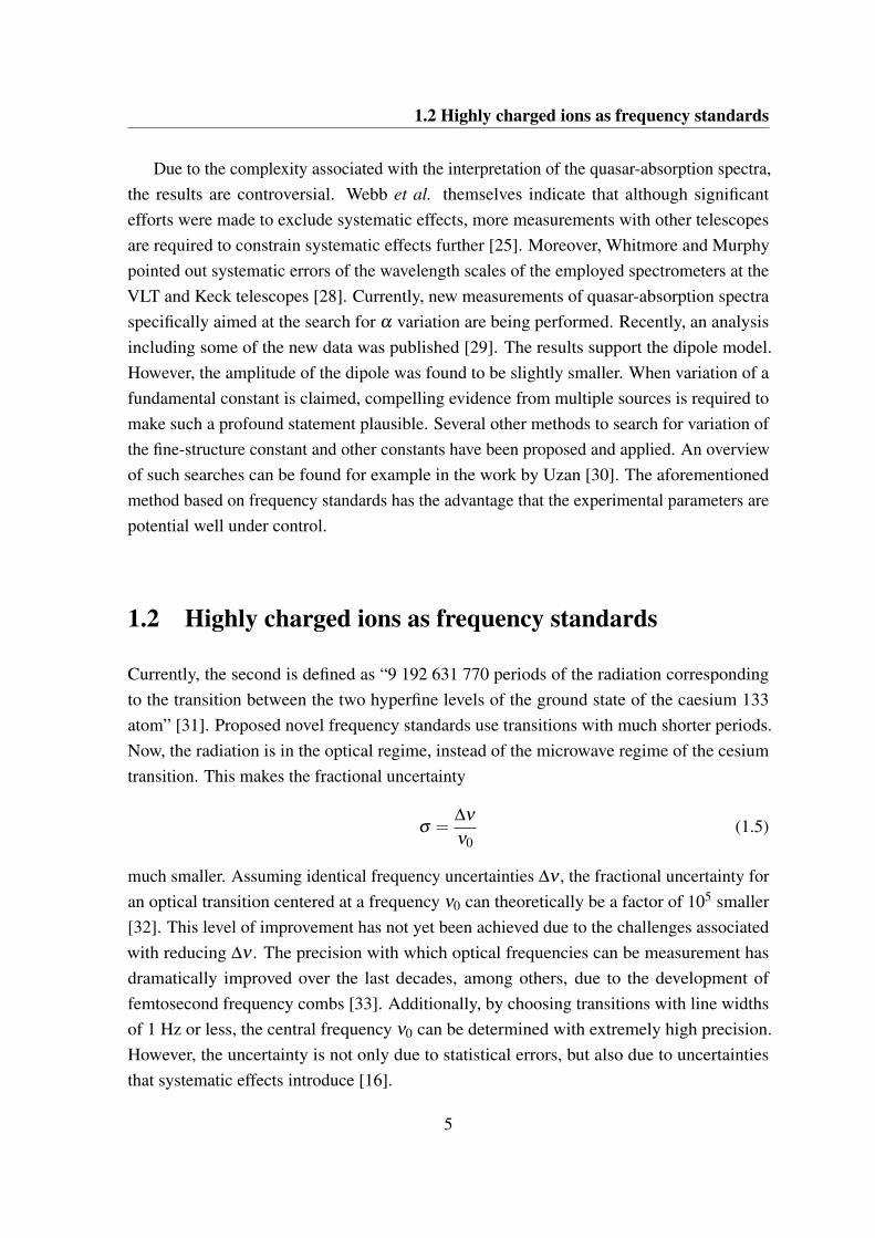
Fig. 1.3 Energy separation between the three lowest energy configurations of the Nd-likesystems with atomic numbers Z = 74−78. The energies are based on Fock-space coupledcluster calculations [34].
The perfect frequency standard would not be perturbed by its environment. Unfortunately,the energy of atomic levels can be shifted by external electric and magnetic fields. For anin-depth discussion of these shifts refer to the publications by Gill [32] and of Ludlow etal. [16], selected sources of shifts are shortly introduced here. Typically, the investigatedions are trapped in a Paul trap which operates by virtue of an AC electric field applied bya set of electrodes. The micromotion of an ion in the electric field causes it to experiencea non-vanishing root-mean-square (RMS) electric field that causes a quadratic Stark shiftof the energy levels. Additional sources of non-vanishing RMS electric fields arise due toblackbody radiation from the environment and due to the laser fields that are employed tointerrogate the ions. Due to imperfections on the surface of the electrodes, a non-vanishingelectric field gradient can exist that couples to the electric quadrupole momenta for certainstates (J > 1/2), which leads to quadrupole shifts of the energy levels. Significant effortsare made to reduce the uncertainty of these systematic effects by precision engineering andcontrol of the setup. However, the systematic shifts are still the largest source of uncertainty.For example, in the Hg+ clock one of the largest uncertainties is due to the quadrupole shift,which causes a fractional uncertainty of 10−17 [17].
The susceptibility of highly charged ions (HCI) to external perturbations is much lowerthan that of the singly charged ions that are employed in current and proposed frequencystandards [35–38]. This is mainly due to the small spatial spread of the electron wave
6
1.2 Highly charged ions as frequency standards
1 0 2 0 3 0 4 0 5 0 6 0 7 0 8 0 9 0 1 0 0
1 0
2 0
3 0
4 0
5 0
6 0
7 0
8 0
1
A t o m i c n u m b e r Z
Cha
rge
stat
e
1 . 0 0 03 . 0 0 05 . 0 0 07 . 0 0 09 . 0 0 01 1 . 0 01 3 . 0 01 5 . 0 01 7 . 0 01 9 . 0 02 1 . 0 02 3 . 0 02 5 . 0 02 7 . 0 02 9 . 0 03 1 . 0 03 3 . 0 03 5 . 0 03 7 . 0 03 9 . 0 04 1 . 0 04 3 . 0 04 5 . 0 04 7 . 0 04 9 . 0 05 0 . 0 0
Squ
are
root
of t
he n
umbe
r of t
rans
ition
s
0
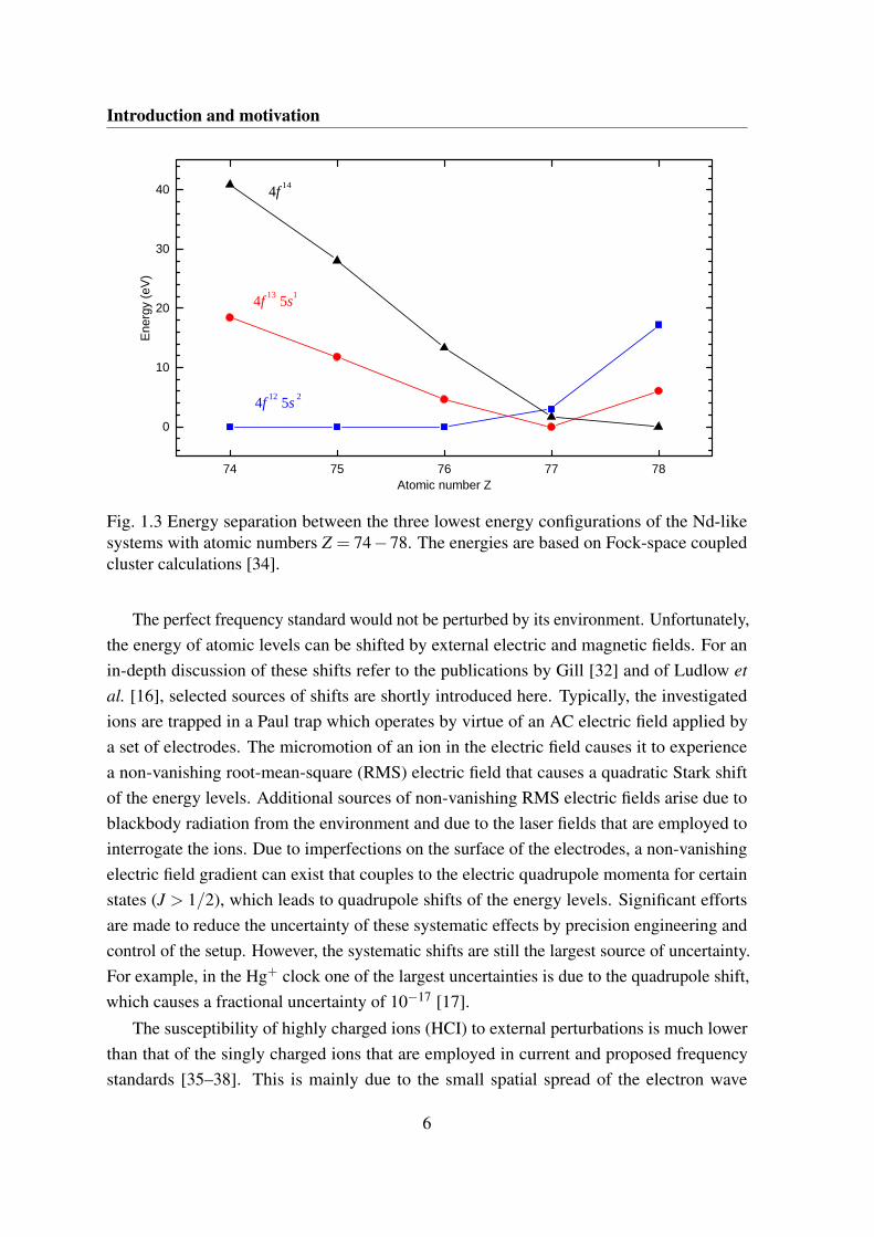
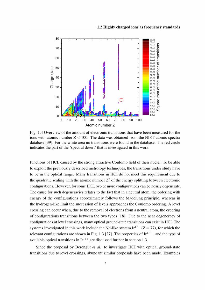
Fig. 1.4 Overview of the amount of electronic transitions that have been measured for theions with atomic number Z < 100. The data was obtained from the NIST atomic spectradatabase [39]. For the white area no transitions were found in the database. The red circleindicates the part of the ‘spectral desert’ that is investigated in this work.
functions of HCI, caused by the strong attractive Coulomb field of their nuclei. To be ableto exploit the previously described metrology techniques, the transitions under study haveto be in the optical range. Many transitions in HCI do not meet this requirement due tothe quadratic scaling with the atomic number Z2 of the energy splitting between electronicconfigurations. However, for some HCI, two or more configurations can be nearly degenerate.The cause for such degeneracies relates to the fact that in a neutral atom, the ordering withenergy of the configurations approximately follows the Madelung principle, whereas inthe hydrogen-like limit the succession of levels approaches the Coulomb ordering. A levelcrossing can occur when, due to the removal of electrons from a neutral atom, the orderingof configurations transitions between the two types [18]. Due to the near degeneracy ofconfigurations at level crossings, many optical ground-state transitions can exist in HCI. Thesystems investigated in this work include the Nd-like system Ir17+ (Z = 77), for which therelevant configurations are shown in Fig. 1.3 [27]. The properties of Ir17+ , and the type ofavailable optical transitions in Ir17+ are discussed further in section 1.3.
Since the proposal by Berengut et al. to investigate HCI with optical ground-statetransitions due to level crossings, abundant similar proposals have been made. Examples
7
Introduction and motivation
include ions such as Sm14+, Sm13+, Pr10+, Nd10+ [36], and Ho14+, Cf15+, Es17+, Es16+
[40]. All these HCI have one or more near ground-state optical transitions with a line widthof 1 Hz or less. Most of those clock transitions also have a high sensitive to the variation ofα . However, all the proposed HCI have a common problem that currently prevents directprecision laser spectroscopy of the clock transitions. Due to a lack of experimental data, thecomplex electronic structure of the proposed HCI is not understood very well. An illustrationof how severe the lack of experimental data is can be seen in Fig 1.4. Furthermore, theprecision of predictions from theory is not good enough for laser spectroscopy. Electronicconfigurations with partially filled nd and n f subshells are extremely complex, since thenumber of possible spin and orbit couplings becomes very large. Calculations of the energylevels are hampered by the intricate electron correlations that are inherent to a level crossing.Even for systems that were specifically selected for their relatively simple electronic structure,the uncertainties on the predicted optical transition wavelengths are a few nm at best [36].This is many orders of magnitude away from what would be needed. To overcome theseproblems, experimental spectral data on HCI near a level crossing are essential: first, to serveas a benchmark to test and improve predictions; second, to determine the wavelengths of theclock transitions with sufficient precision so that laser spectroscopy can be performed.
1.3 Ir17+ as a highly sensitive detector of variation of thefine-structure constant
The sensitivity of a transition to the variation of α was previously parametrized by thefactor q. Equivalently to equation (1.2), for the energy of a fine-structure level the sensitivitycan be defined. For the energy of electrons above closed shells, it can be shown that [41, 42]
q ≈−In(Zα)2
ne( j+1/2). (1.6)
Here, In = Z2e/2n2
e is the ionization energy of the electron, Ze is the effective nuclear chargethat the electron experiences, ne the associated effective principle quantum number, and jthe total angular momentum quantum number. In shells that are nearly full, the screeningof the nuclear charge Z is less effective. For those type of systems, the contribution of theionization energy to the q factor is enhanced, so that q ∝ I3/2
n [27]. Hence, systems with alarge nuclear charge and with configurations with nearly filled shells provide the highestsensitivity to the variation of α . Guided by this, and by the restriction that the transitionshave to be in the optical range, Berengut et al. proposed Ir17+ among other systems [27].
8
1.3 Ir17+ as a highly sensitive detector of variation of the fine-structure constant
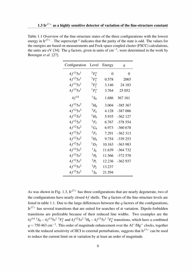
Table 1.1 Overview of the fine-structure states of the three configurations with the lowestenergy in Ir17+ . The superscript o indicates that the parity of the state is odd. The values forthe energies are based on measurements and Fock-space coupled cluster (FSCC) calculations,the units are eV [34]. The q factors, given in units of cm−1, were determined in the work byBerengut et al. [27].
Configuration Level Energy q
4 f 135s1 3Fo4 0 0
4 f 135s1 3Fo3 0.578 2065
4 f 135s1 3Fo2 3.146 24 183
4 f 135s1 1Fo3 3.764 25 052
4 f 14 1S0 1.686 367 161
4 f 125s2 3H6 3.004 -385 3674 f 125s2 3F4 4.128 -387 0864 f 125s2 3H5 5.935 -362 1274 f 125s2 3F2 6.767 -378 5544 f 125s2 1G4 6.973 -360 6784 f 125s2 3F3 7.291 -362 3134 f 125s2 3H4 9.754 -339 2534 f 125s2 1D2 10.163 -363 9834 f 125s2 1J6 11.639 -364 7324 f 125s2 3P0 11.566 -372 5704 f 125s2 3P1 12.236 -362 9374 f 125s2 3P2 13.2374 f 125s2 1S0 21.594
As was shown in Fig. 1.3, Ir17+ has three configurations that are nearly degenerate, two ofthe configurations have nearly closed 4 f shells. The q factors of the fine-structure levels arelisted in table 1.1. Due to the large differences between the q factors of the configurations,Ir17+ has several transitions that are suited for searches of α variation. Dipole-forbiddentransitions are preferable because of their reduced line widths. Two examples are the4 f 14 1S0 – 4 f 135s1 3Fo
3 and 4 f 125s2 3H6 – 4 f 135s1 3Fo4 transitions, which have a combined
q = 750 463 cm−1. This order of magnitude enhancement over the Al+/Hg+ clocks, togetherwith the reduced sensitivity of HCI to external perturbations, suggests that Ir17+ can be usedto reduce the current limit on α variation by at least an order of magnitude.
9
Introduction and motivation
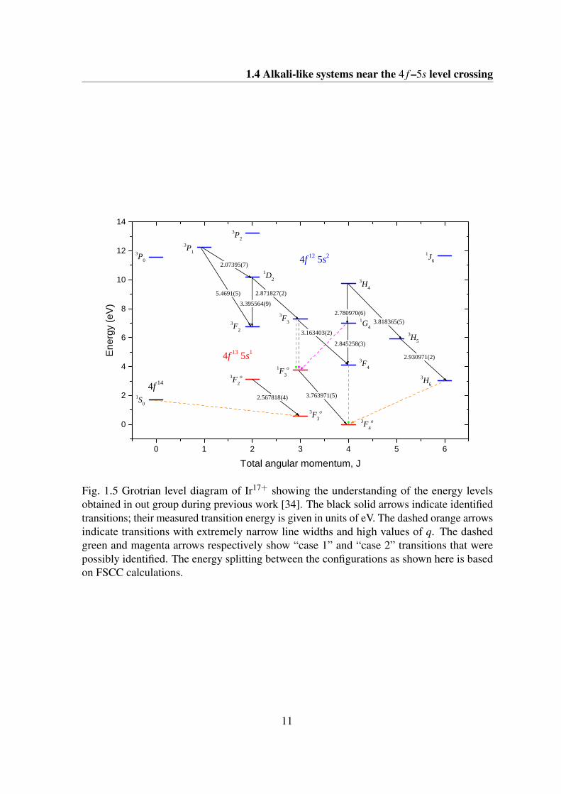
Soon after the proposal in 2011 to use Ir17+ as a system to search for variation ofthe fine-structure constant, an experimental investigation of this ion was started at theMax Planck Institute for Nuclear Physics in Heidelberg. The Heidelberg electron beam iontrap (HD-EBIT) was employed to produce and trap the Ir17+ ions. Emission spectra ofIr17+ and other ions in the Nd-like sequence (Z = 74–78) were measured using a gratingspectrometer that was sensitive in the optical range. Due to the large number of measuredspectral lines and the uncertainties associated with the predictions, a direct identification oflines was not possible. However, due to the availability of spectra from multiple Nd-likesystems and by employing several analysis techniques, a number of transitions taking placewithin configurations could be identified. An overview of them is shown in Fig. 1.5. Moreover,some yet unidentified lines were found to form, within the measurement uncertainty, closedoptical cycles. Two of those closed cycles include candidates for transitions between theconfigurations. Since the two cycles (named case 1 and case 2) were mutually exclusive,no definitive conclusion regarding the energy splitting between the 4 f 135s1 and 4 f 125s2
configurations could be drawn. Therefore, the sought-after wavelengths of the 3H6 – 3Fo4
and 1S0 – 3Fo3 transitions could not be ultimately determined. In this work the electronic
structure of Ir17+ is investigated through measurements of emission spectra in the EUV range.Furthermore, spectra with increased precision compared to previous measurements weretaken of several lines belonging to case 1 and 2.
1.4 Alkali-like systems near the 4 f –5s level crossing
The elements in the alkali group of the periodic table have been subject to extensive studybecause of their relatively simple electronic structure with a single ns electron outside closedshells. For the same reason, singly charged ions of the alkaline earth metals are the mainsubject of many experiments in atomic physics. In the realm of highly charged ions (HCI) toothere is considerable interest in alkali-like ions, for example, the 2s - 2p transitions in Li-likePr were studied recently as a means to access nuclear properties through the level splittingsinduced by the nuclear magnetic field [43]. A wide range of Na-like ions was investigated inthe extensive work of Gillapsy and co-workers 3s - 3p [44]. The next iso-electronic sequencethat has been investigated for its 4s - 4p transitions is not so much the K-like sequence butthe Cu-like sequence, because a level crossing of the 4s and 3d configurations brings a single4s electron above a closed 3d10 shell [45]. Similarly, level crossings make that the Pm-likeiso-electronic sequence has a single 5s electron above a closed 4 f 14 shell. Curtis and Elliswere the first to publish on their theoretical investigation of Pm-like HCI [46].
10
1.4 Alkali-like systems near the 4 f –5s level crossing
0 1 2 3 4 5 6
0
2
4
6
8
1 0
1 2
1 4
4 f 1 2 5 s 2
4 f 1 3 5 s 1Ene
rgy
(eV
)
T o t a l a n g u l a r m o m e n t u m , J
1 S 0
3 P 23 P 13 P 0
1 J 6
1 D 2 3 H 4
1 G 4
3 F 33 F 2
3 F 4
3 H 5
3 H 6
1 F 3o
3 F 2o
3 F 3o
3 F 4o
3 . 1 6 3 4 0 3 ( 2 )
3 . 3 9 5 5 6 4 ( 9 )
3 . 7 6 3 9 7 1 ( 5 )
2 . 0 7 3 9 5 ( 7 )
5 . 4 6 9 1 ( 5 ) 2 . 8 7 1 8 2 7 ( 2 )
2 . 7 8 0 9 7 0 ( 6 )
2 . 8 4 5 2 5 8 ( 3 )
3 . 8 1 8 3 6 5 ( 5 )
2 . 9 3 0 9 7 1 ( 2 )
2 . 5 6 7 8 1 8 ( 4 )4 f 1 4
Fig. 1.5 Grotrian level diagram of Ir17+ showing the understanding of the energy levelsobtained in out group during previous work [34]. The black solid arrows indicate identifiedtransitions; their measured transition energy is given in units of eV. The dashed orange arrowsindicate transitions with extremely narrow line widths and high values of q. The dashedgreen and magenta arrows respectively show “case 1” and “case 2” transitions that werepossibly identified. The energy splitting between the configurations as shown here is basedon FSCC calculations.
11

Chapter 2
Theory
One, two, many.
— Counting system of primitive tribes such as the Pirahã
A detailed treatise of atomic physics will not be given here, as that can be found inmany textbooks (refer to citations throughout this chapter). Nonetheless, important equationsand scaling laws necessary for a better understanding of the contents of this work will beintroduced and discussed. Attention is given to important processes taking place in an EBIT.Subsequently, an introduction to the computational methods and tools employed to interpretthe measurements made in the course of this work are given.
2.1 Basics of Atomic Physics
For a proper description of the properties of an atom, the theory of quantum physics isrequired [47–49]. In quantum physics, the system under study is completely described by awave function Ψ(t). To find the wave function the Schrödinger equation must be solved,
ih∂
∂ tΨ(t) = HΨ(t). (2.1)
The Hamiltonian H, which acts on the wave function, needs to include all the interactionstaking place in the system for a proper description. Solving the Schrödinger equation fora specific system is analogous to using Newton’s second law of motion to determine thedynamics of a classical system. The values that observables can take are given by actingon the wave function with the appropriate operator. For example, the Hamiltonian operator
13
Theory
gives the energies Ei that the system can have as
HΨ(t) = EiΨ(t). (2.2)
2.1.1 Hydrogen-like systems
One of the simplest atomic systems is the hydrogen-like system, i.e. a nucleus of charge Zewith a single bound electron. The Hamiltonian for such a system is given by
HBohr =−h2
2me∇
2 − Ze2
4πε0r. (2.3)
The first term takes into account the kinematics of the system based on the theory of Bohr.The second term accounts for the Coulomb interaction between the electron and the nucleusof charge Ze. Due to the spherical symmetry of the system it is convenient to work inspherical coordinates when solving the Schrödinger equation. The wave function is then splitinto a radial and an angular component as Ψ(r) = R(r)ϒ (θ ,φ). Solutions of the Schrödingerequation with HBohr predict the gross structure of the energy levels to be
E(n) =− meZ2e4
32(πε0)2n2 , n = 0,1,2, ... (2.4)
The principal quantum number n represents the quantization of the radial part of the system.Physicists in the 1920’s employed perturbation theory to apply several small corrections toHBohr. These corrections account for the quantization of the orbital angular momentum andleading relativistic effects. The energy levels are then predicted to be
E(n, l)≈−E(n)
[1+
Z2α2
n2
(n
l + 12
− 34
)](2.5)
to a good approximation. The quantum number l is associated with the orbital angularmomentum. This lifts the degeneracy of levels with the same principal quantum number ninto l < n sublevels. The added structure is known as the fine structure. From equation (2.5)it follows that the size of the fine-structure splitting scales with Z4, so in highly charged ions(HCI) the splitting can easily be in the keV range. But under certain conditions, as discussedin chapter 1, near level crossings the energy difference between fine-structure levels can bein the eV range.
The main problem with the Hamiltonian introduced in equation (2.3) is that it is intrinsi-cally not relativistic [50]. This can be seen for example by the fact that the second derivative
14
2.1 Basics of Atomic Physics
with respect to spatial coordinates is taken, while in the Schrödinger equation only the firstorder derivative of the time coordinate is taken. Dirac solved this problem by introducing thefollowing Hamiltonian [51],
HDirac = βββmec2 + cααα
(−ih∇− e
cA)+ eΦ. (2.6)
A full description of this Hamiltonian is beyond the scope of this work. However, it isapparent that this Hamiltonian, when substituted in the Schrödinger equation, treats thespatial and temporal coordinates alike. The resulting equation is generally known as theDirac equation. The wave functions that are found when solving the Dirac equation areconstructed from Dirac spinors ϕn, j,m [50].
In the Dirac Hamiltonian the electromagnetic interaction is included in relativistic form bythe electric potential φ and the vector potential AAA. Moreover, it describes the spin of electronswith the Dirac matrices ααα and βββ . The spin of an electron behaves mathematically similarlyas the orbital angular momentum of the electron. Each angular momentum observable hasits own quantum number, l for orbital angular momentum and s = 1/2 for spin angularmomentum. These couple to a total angular momentum of j = |l − s|...|l + s| which can besubstituted for l in equation (2.5) to obtain the approximate energy levels. It is customary towrite the state of the system in term notation,
2s+1l j. (2.7)
Here for l the spectroscopic notation s = 1, p = 2, d = 3, et cetera is used.
Further refinements to the energy levels of hydrogen-like systems can be made byconsidering quantum electrodynamic (QED) effects. An example is the interaction of theelectron with virtual particle anti-particle pairs created by vacuum polarization. In strongelectromagnetic fields the probability to create these virtual particle pairs is increased. Theelectric field that the electron in a hydrogen-like system experiences scales with Z3, so forheavy HCI these effects start to play an important role. However, the systems investigated inthis work are not charged highly enough to have an appreciable effect on the measurements.
2.1.2 Many-electron systems
Solving the Schrödinger equation for systems with more than one electron is not analyticallypossible anymore. The electrons interact not only with the nucleus, but also with each other,
15
Theory
so that the Hamiltonian turns into
HMB = ∑i
HDirac,i +∑i< j
e2
|rrri − rrr j|. (2.8)
Here, the sums are understood to be taken over all the electrons in the system. Computationalmethods to calculate the energy levels and to obtain the wave function of the system arediscussed in section 2.3. Here general principles regarding the electronic structure of many-electron systems are discussed.
Since electrons have half integer spin (i.e. they are fermions) they obey the Pauli exclusionprinciple. Therefore, each electron has to be in a state with distinct quantum numbers n, j,m j (m j is the z-component of the angular momentum). Electrons with the same principalquantum number n are said to be in the same shell. A shell can consist of several subshells,which are defined by the angular momentum quantum number j. Many-electron systemscan have multiple shells that are fully or partially filled with electrons. The notation for theelectronic configuration of an atom is a sequence of nlx, where x is the number of electronsin the subshell. For example, neutral boron in the ground state has the electron configuration1s22s22p1. Note that when x = 1 it is sometimes omitted.
The angular momenta of the electrons can couple in two different ways. The Russell-Saunders regime is where the coupling between the orbital l and spin s angular momenta ofindividual electrons is weak compared to the coupling between the orbital angular momentaand the electron spins. The individual l’s can then couple to form the total orbital angularmomentum L = ∑i li, similarly for the total spin S = ∑i si. Those couple to form the totalangular momentum J = L+S. Again, the state of the system is usually given in the termnotation which was introduced in equation 2.7. Enhanced relativistic effects increase thestrength of the spin-orbit coupling in high Z atoms. In that case the orbital l and spin sangular momenta of individual electrons couple to form the total angular momentum of asingle electron j. These individual total angular momenta couple to form the total angularmomentum J =∑i ji. Thus, the total angular momenta L and S are not good quantum numbersanymore. In both cases, the total angular momentum J is a good quantum number that isimportant for a lot of the properties of the electronic structure. Additionally, the selectionrules for transitions are governed in part by the J’s of the involved states, more on that insection 2.1.5. Therefore, the Grotrian level diagrams in this work are often shown to have thevalues for the total angular momentum on the x-axis.
The nucleus can also have spin which interacts with the electrons, this gives rise to ahyperfine structure of the fine-structure levels. Since this effect scales with α2Z3/n3 thehyperfine transitions can be in the optical range for HCI, such as for example in hydrogen-like
16
2.1 Basics of Atomic Physics
rhenium [52]. In Ti-like Re53+ however the hyperfine splitting is in the order of 1 meV dueto the n3 dependence and the screening of the nucleus [53]. The two naturally occurringisotopes of iridium 191Ir and 193Ir both have a nuclear spin I = 3/2 with nuclear magneticmomenta of respectively 0.1461 µN and 0.1591 µN [54]. This is approximately 20 timeslower than that of 185Re and 187Re. Moreover, the valence electrons in Ir17+ have a higherprincipal quantum number and are more strongly screened by the closed shells. Hencethe hyperfine splitting in Ir17+ is negligible compared to other effects, such as the Zeemansplitting which is discussed next.
2.1.3 The Wigner-Eckart theorem
When working with angular momentum eigenstates, the Wigner-Eckart theorem is a powerfultool to calculate expectation values of other operators [47]. In the next section this theoremis necessary to calculate the relative intensities of transitions. The theorem applies to systemswith eigenstates | jm⟩. In such a basis the expectation value of a general spherical tensoroperator T k of rank k is
⟨ j′m′|T kq | jm⟩= ⟨ jmkq| j′m′⟩⟨ j′||T k|| j⟩. (2.9)
Here q denotes the component of the operator. ⟨ j′m′kq| jm⟩ is the Clebsch-Gordan coefficientfor coupling j with k to get j′, its value can be looked up in for example the Review ofParticle Physics [55]. ⟨ j′||T k|| j⟩ is the reduced matrix element, which does not depend on m,m′, and q.
A specialized form of the Wigner-Eckart theorem called the projection theorem is intro-duced here too. It is valid for rank 1 spherical tensor operators V defined by their commutationrelation
[V i,J j] = iεi jkJk. (2.10)
The projection theorem states that the expectation value of vector operators is proportional tothe expectation value of J.
⟨ jm′|V| jm⟩= ⟨ jm′|V ·J| jm⟩j( j+1)
⟨ jm′|J| jm⟩. (2.11)
2.1.4 Zeeman splitting
Even before the theory of quantum mechanics started to be developed, many quantum effectswere observed experimentally. An example is the Zeeman effect, reported in 1897 by the
17
Theory
Dutch physicist Pieter Zeeman [56]. He observed that spectral lines are split into multiplecomponents when the emitting medium is exposed to an external magnetic field. Since theions investigated in this work were exposed to the strong magnetic field of the EBIT, theZeeman effect needs to be taken into account.
Neglecting nuclear spin effects, which are a factor mp/me ⋍ 1836 smaller, the atomicmagnetic moment is given by
µµµ =−µBL−gsµBS. (2.12)
Here µB = eh/2me is the Bohr magneton, for which the CODATA recommended valueµB = 5.7883818012(26) ·10−5 eV /T was taken [13]. The Hamiltonian for a magneticmoment in an external magnetic field B = Bzez is given by
HZE =−µµµ ·B = µBBz(Lz +gsSz). (2.13)
As it turns out, for the magnetic field strengths applied in this work, the effect is small enoughso that it can be treated as a perturbation of the spin-orbit interaction. The correction to theenergy is then
∆EZE = ⟨ jmls|HZE| jmls⟩ (2.14)
= µBBz⟨Lz +gsSz⟩
= µBBz⟨L ·J⟩+gs⟨S ·J⟩
j( j+1)⟨Jz⟩
= µBBzg jm j.
For legibility, the eigenstate quantum numbers are omitted from line two onward. The thirdline is obtained by application of the projection theorem. In the final step the Landé g-factoris defined as
g j ≡ 1+(gs −1)j( j+1)− l(l +1)+ s(s+1)
2 j( j+1). (2.15)
Inclusion of the Breit interaction and QED effects can change this g j-factor from the thirddigit on.
2.1.5 Zeeman transitions
When an atomic system transitions between two energy levels the excess energy can bereleased in the form of a photon. In this work, the wavelength of the emitted photons
18
2.1 Basics of Atomic Physics
was measured to gain insights about the electronic structure of ions. The transition energybetween two fine-structure levels is given by
∆E = E i +∆E iZE −E f −∆E f
ZE (2.16)
= ∆EFS +∆EZE.
The superscripts denote the initial i state and the final f state. Equation (2.14) shows that theenergy of a fine-structure level in a magnetic field Bz is split into 2 j+1 sub-levels. Thus afine-structure transition is split into a number of transitions with energies slightly deviatingfrom the central wavelength ∆EFS. The energy differences from the central wavelength aregiven by
∆EZE = µBBz(gijm
ij −g f
j m fj ) (2.17)
= µBBzmij(g
ij −g f
j ) for ∆m = 0
= µBBz(mij(g
ij −g f
j )±g fj ) for ∆m =±1.
The division into ∆m = mi −m f groups is in anticipation of the selection rules which will beintroduced below. The equations (2.17) show that the energy splitting between the Zeemantransitions is determined by gi
j −g fj , and the splitting between the ∆m groups by g f
j , refer toFig. 2.1.
To compare the predicted splitting with observations, it is necessary to determine therelative intensities of the transitions between the Zeeman sub-levels. Transitions ratesbetween an initial state |i⟩ and final state | f ⟩ separated by an energy E can be calculatedusing Fermi’s golden rule
Ai f ∝ E3⟨ f |T |i⟩2. (2.18)
Here the interaction between the states is governed by the operator T . In the electric dipoleapproximation the operator is simply −er. With the quantization axis defined by the B-fieldin the z-direction, the dipole operator can be written as the spherical tensor operator Dq ofrank 1
D1 =− e√2(rx + iry) (2.19)
D0 = erz
D−1 =− e√2(rx − iry).
19
Theory
Now, to find the relative intensity of a Zeeman transitions between two fine-structure levels| jimi⟩ and | j f m f ⟩
Ai f ∝ ⟨ j f m f |Dq| jimi⟩2 (2.20)
= ⟨ j f m f 1q| jimi⟩2⟨ j f ||D|| ji⟩2
= ⟨ j f (mi +∆m)1∆m| jimi⟩2⟨ j f ||D|| ji⟩2, ∆m = 0,±1.
In the first step the Wigner-Eckart theorem is applied. The second step follows from the factthat the Clebsch-Gordan coefficients are only non-zero when q+mi −m f = 0. Furthermore,the reduced matrix element is equal for all the Zeeman transitions between the fine-structurelevels. So the relative intensities of the Zeeman components only depend on the Clebsch-Gordan coefficients. In similar vein as the selection rule for the ∆m’s, it follows that∆ j = 0,±1. However, j = 0 → j′ = 0 transitions are not allowed. And finally, since theelectric dipole operator is odd with respect to parity transformations, electric dipole (E1)transitions can only take place between states of opposite parity.
Similarly to the derivation of the relative intensities and selection rules for E1 transitions,it is possible to derive these for magnetic dipole (M1) transitions. The interaction operatorin that case is the magnetic moment from equation (2.12). Only a few selection rules aredifferent compared to E1 transitions. Because the magnetic moments operator is even withrespect to parity transformations, M1 transitions only take place between states of the sameparity. The interaction due to the magnetic dipole operator is much weaker then that of theelectric dipole operator
⟨µµµ ·B⟩2
⟨er ·E⟩2 ∼ (µB/cea0/Z
)2 ∼ (αZ)2. (2.21)
Since the total rate in (2.18) grows with E30 , in HCI the rate of M1 transitions scales with Z10
whereas E1 transition rates scale with Z4. Hence, M1 transitions in the optical regime can beas strong as, or even stronger than E1 transitions.
The angular distribution of the emitted photons can be deduced by considering the formof the dipole operator in spherical tensor form, equation (2.20), and the ∆m selection rules.For ∆m = 0 the system behaves as a linear oscillator in the z-direction. And for ∆m =±1the ion behaves as a circular oscillator in the xy-plane. The radiation pattern then follows
20
2.1 Basics of Atomic Physics
E 0
- 3- 2- 1012
3 F 3
Ene
rgy
(arb
. uni
ts)
1 F o3
3
- 3- 2- 10123m j =
E 0
π|| π⊥
Inte
nsity
(arb
. uni
ts)
E n e r g y ( a r b . u n i t s )
π⊥
g ij - g j
f
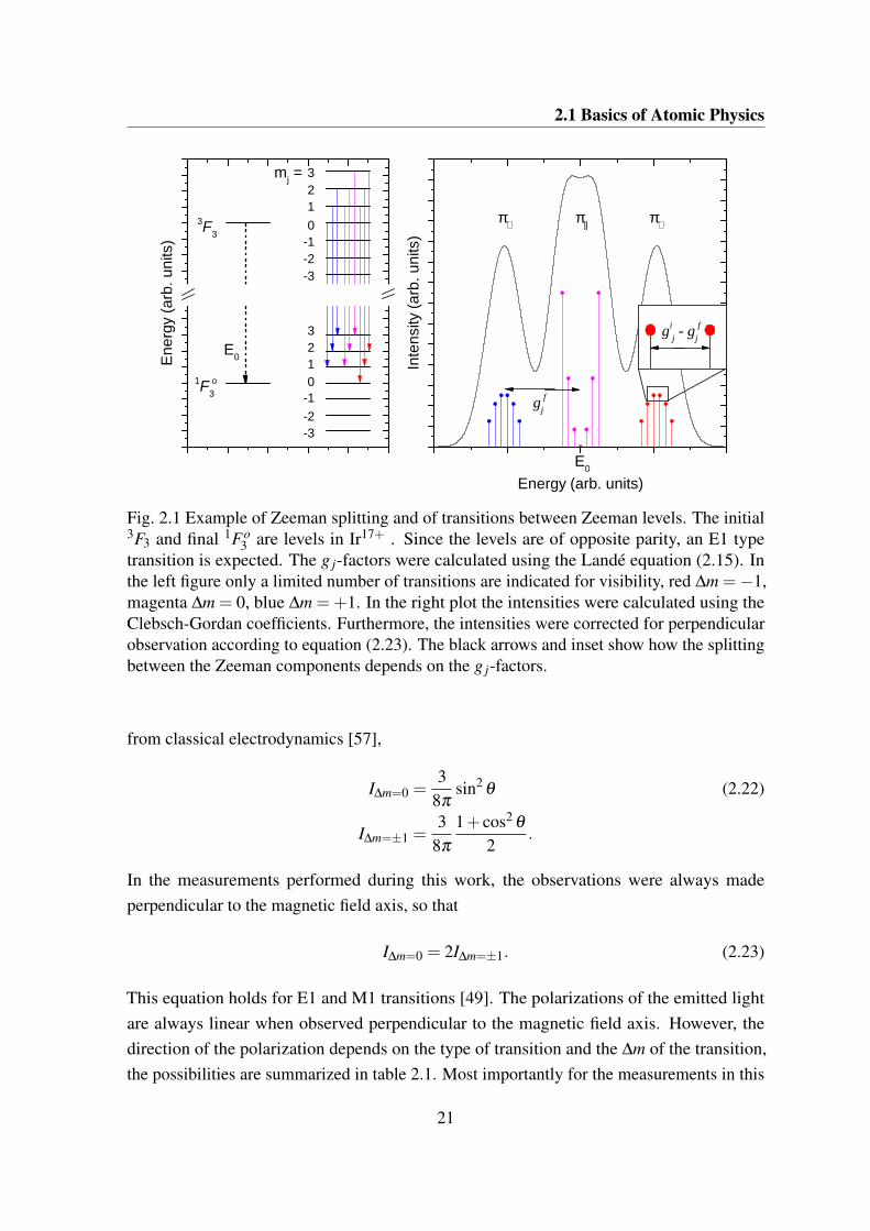
g jf
Fig. 2.1 Example of Zeeman splitting and of transitions between Zeeman levels. The initial3F3 and final 1Fo
3 are levels in Ir17+ . Since the levels are of opposite parity, an E1 typetransition is expected. The g j-factors were calculated using the Landé equation (2.15). Inthe left figure only a limited number of transitions are indicated for visibility, red ∆m =−1,magenta ∆m = 0, blue ∆m =+1. In the right plot the intensities were calculated using theClebsch-Gordan coefficients. Furthermore, the intensities were corrected for perpendicularobservation according to equation (2.23). The black arrows and inset show how the splittingbetween the Zeeman components depends on the g j-factors.
from classical electrodynamics [57],
I∆m=0 =3
8πsin2
θ (2.22)
I∆m=±1 =3
8π
1+ cos2 θ
2.
In the measurements performed during this work, the observations were always madeperpendicular to the magnetic field axis, so that
I∆m=0 = 2I∆m=±1. (2.23)
This equation holds for E1 and M1 transitions [49]. The polarizations of the emitted lightare always linear when observed perpendicular to the magnetic field axis. However, thedirection of the polarization depends on the type of transition and the ∆m of the transition,the possibilities are summarized in table 2.1. Most importantly for the measurements in this
21

Theory
Table 2.1 Overview of the polarizations of fluorescence light from Zeeman transitions asobserved either parallel or perpendicular to the magnetic field axis [49]. The light can becircularly polarized σ±, linear parallel to the magnetic field axis π⊥, or linear perpendicularto the magnetic field axis π∥.
E1 M1∆m Parallel Perpendicular Parallel Perpendicular+1 σ− π⊥ - π∥0 - π∥ σ± π⊥-1 σ+ π⊥ - π∥
work, the polarization direction for the ∆m = 0 and ∆m =±1 transitions switches dependingon the transition being either E1 or M1. An example for the line shape of an Ir17+ transitiondue to all the aforementioned effects is shown in Fig. 2.1, more predicted line shapes forIr17+ are given in appendix A.
2.2 Electron-ion interactions in an EBIT
The ions studied in this work were produced and trapped in an electron beam ion trap (EBIT).As the name suggests, in the EBIT an electron beam interacts with ions. Typically anywherefrom 104 to 107 ions are trapped in a cylindrical volume of a few centimeter in length andapproximately 500 µm in diameter. A more comprehensive discussion of the EBIT is givenin chapter 3. In this section, the significant processes taking place in an EBIT are introducedand given theoretical background.
In an EBIT, sequential ionization to higher charge states is accomplished through electronimpact ionization. In this process, an ion A of charge state q and in quantum state a interactswith an energetic electron. If the electron is energetic enough it can transfer part of its kineticenergy to the ion and thereby eject a bound electron from the ion,
Aqa + e− → Aq+1
b +2e−. (2.24)
At the end of the interaction the ion is left in the next higher charge state q+1 and quan-tum state b. The cross section in units of cm2 for this process can be estimated with thesemiempirical equation proposed by Lotz [58],
σEIIqa = 4.5×10⁻¹⁴
∑i
ξiln(Ee/Iiab)
EeIiab. (2.25)
22
2.2 Electron-ion interactions in an EBIT
Here the ξi is the number of equivalent electrons in the subshell of the initial quantum state.Obviously the electron energy Ee needs to be as large, or larger then the ionization energyIiab required to bring the ion to the state Aq+1
b . As a rule of thumb, the Lotz equation predictsthat the maximum electron impact ionization cross section is at approximately 2.5 times theionization energy Iiab. Since high energetic states are usually short lived (c.f. equation (2.18))with respect to the rate of electron impact ionization, often only the ionization from theground state needs to be considered. However, in some cases long lived meta-stable statesexist that allow for efficient ionization even though Ee does not exceed the ionization energyof the ground state yet [59].
Electron impact not only causes ionization, it can also directly bring the atom to anotherquantum state,
Aqa + e− → Aq
b + e−. (2.26)
When the ion is brought to an energetically higher state this is know as excitation, otherwiseit is know as de-excitation or quenching. Electron impact excitation can occur only whenthe electron beam energy Ee is equal to, or higher, than the energy difference between theinitial and final states Ei f . The cross section for excitation of ions (not that of atoms) hasits maximum at threshold, that is, when Ee = Ei f . For dipole transitions the cross section atmuch higher energies decreases as [60, 61]
σEIE ≈ A
Ee+B
lnEe
Ei fEe ≫ Ei f . (2.27)
Here A and B are constants. The value for the cross section in units of cm2 at threshold canbe approximated by the semiempirical van Regemorter equation [62],
σEIEmaximum ≈ 4.72−18
E2i f
, (2.28)
with Ei f in eV. In general the electron impact ionization cross section is much larger thanthe cross section for excitation. Therefore, only when the electron beam energy is near theionization energy of an ion will excitation play a role. At that point the electron beam energyis so high that mainly states with a high principal quantum number n are populated. The ionsubsequently relaxes though multi-step radiative decay.
Photon ionization and excitation is not discussed in this work since the cross sections forthese processes are relatively small and the photon density during the measurements was low.Only when intense radiation from an external source is introduced, does the need to consider
23
Theory
photon excitation and ionization arise. This is for example the case when the radiation froma free electron laser (FEL) is overlapped with the ion sample [63].
The inverse process of ionization, recombination of an electron with an ion, also occursin the EBIT. The simplest recombination process is radiative recombination (RR), in which afree electron recombines with an ion and the excess energy is directly emitted in the form ofa photon,
Aqa + e− → Aq−1
b + γ. (2.29)
Though electron-electron interactions there are instances when the excess energy can excitealready bound electrons to a higher energetic state. Only in the next step is the excess energyradiated away, so that the total process can be described as
Aqa + e− → Aq−1
b → Aq−1c + γ. (2.30)
In the most common form of this process only one bound electron is raised to a higherstate, in which case the process is known as dielectronic recombination. Since the excessenergy has to be equal to the energy required for the excitation of the bound electrons,this is a resonant process. Recombination processes are extensively studied in the EBITcommunity, predominantly with the goal of providing data to model astrophysical object,refer for example to the review by Beiersdorfer [64]. Recombination processes to the L-shellof iridium were investigated by Hollain to gain a better understanding of the electronicstructure of this element [65].
2.3 Computational methods in atomic physics
Over the course of this the work predictions from the lexible atomic code (FAC) wereextensively used to interpret the performed measurements. The abilities of FAC includethe calculation of atomic properties such as the energies of fine-structure levels, transitionrates, and collisional excitation cross sections. Additionally, the libraries include a moduleto perform collisional radiative modeling of plasmas. The code was developed by M. F. Gu,who also published a review describing the basic functionality [66]. The advantages ofFAC are its user friendliness and that most calculations can be performed in limited time onpersonal computer systems. In general, the results are accurate enough to identify lines inspectra. For example, predictions for the wavelengths of L-shell transitions were proven tobe accurate at the level of 0.1% [67, 68].
24
2.3 Computational methods in atomic physics
Several numerical methods exist to solve the Schrödinger equation and thereby obtaina good approximation of the wave function. All the methods described here use the Dirac-Coulomb-Breit Hamiltonian
HDCB = ∑i
HDirac,i +∑i< j
e2
|rrri − rrr j|+Bi j. (2.31)
Which is equal to the Hamiltonian introduced in equation (2.8) plus the Breit operator Bi j [69].The Breit operator partially takes into account retardation effects and magnetic interactionsbetween the electrons. In FAC, a configuration interaction (CI) method is implemented. Thismethod is also the basis for the results provided by N. S. Oreshkina. The results providedby A. Borschevsky were obtained using a coupled cluster (CC) method. Both methods arediscussed shortly in the next section. Subsequently, an introduction to the collisional radiativemodel (CRM) is given.
2.3.1 The configuration interaction method
The wave function of a specific state of an N electron system can be described by configu-ration state functions (CSF). These are the antisymmetritrized products of N one-electronwave functions. The antisymmetric condition is required so that the Pauli principle is upheld.Usually, the Slater determinant
φ =1√N!
∣∣∣∣∣∣∣∣∣ϕ1(a1) · · · ϕN(a1)
... . . . ...
ϕ1(aN) · · · ϕN(aN)
∣∣∣∣∣∣∣∣∣ (2.32)
is introduced to mathematically represent antisymmetritrized product. The ϕi(ai) representsolutions of the one-electron Dirac equation with quantum numbers ai. In the configurationinteraction Dirac-Fock-Sturmian (CIDFS) method as applied by N. S. Oreshkina, the ϕi(ai)
for occupied orbitals are obtained from a multiconfiguration Dirac-Fock calculation [70, 71].The one-electron wave functions for correlation orbitals were constructed from Sturmianbasis functions.
The full solution to the multi-electron Dirac equation is a superposition of the CSF,
Ψ = ∑i
biφi. (2.33)
25
Theory
Ideally, the sum would be taken over all the possible configuration state functions φi. In theconfiguration interaction method the coefficients bi are varied to yield the minimal energyfor the system,
E = ⟨Ψ|H|Ψ⟩= ∑i
bi⟨φi|H|φi⟩. (2.34)
For systems with many electrons it is often too computationally expensive to take the sumover all CSF, then the sum is truncated. Typically, the CSF are categorized according to thenumber of electrons excited from the ground state. For example, the CIDFS calculationswere performed for a CSF basis of single excitations up to the 7s, 7p, 7d, and 7 f subshellsand double excitations up to the 5p subshells. Even with such a relatively large basis andcorresponding cost in computational time, the results did not show convergent behavioryet. Therefore, the uncertainty on the energies of the configurations was estimated tobe approximately 1 eV. The uncertainty on the energy of fine-structure levels within aconfiguration was estimated to be at the level of 1% [72].
2.3.2 The coupled cluster method
In the coupled cluster method a different form for the full wave function is chosen, namely
Ψ = eTφ0. (2.35)
Here φ0 is the CSF for the ground state of the system, and T is the so-called cluster opera-tor [73]. The cluster operator is the sum of excitation operators,
T = ∑i
Ti. (2.36)
The subscript i denotes how many excitations are produced by the operator. The generalform of the cluster operator is given by
Tn =1
(n!)2 ∑h1···hn
∑p1···pn
th1···hnp1···pn
ap1 · · ·apnah1 · · ·ahn. (2.37)
Here the a denote creation and annihilation operators for occupied orbital h and unoccupiedorbital p. The coefficients t are found by inserting the Hamiltonian (2.31) and the wavefunction (2.35) in the Schrödinger equation and solving for t [73].
The calculations performed by A. Borschevsky were limited to include up to doubleexcitations. With this in mind, the exponential part of equation (2.35) can be expanded in a
26
2.3 Computational methods in atomic physics
Taylor series,
eT = 1+T +12!
T 2 + · · · (2.38)
= 1+T1 +T2 +12
T 21 +T1T2 +
12
T 22 + · · ·
Although only excitation operators up to T2 are considered, contributions of higher orderexcitations are also partly included by terms such as for example T1T2 for triple excitations.This makes the CC method very suited for calculations on highly correlated systems such asthose studied in this work. The specific code used for the calculations by A. Borschevskywas written by E. Eliav, U. Kaldor, and Y. Ishikawa [74]. In the code, the ground state CSF φ0
is found by a method based on the Dirac-Fock basis expansion [75]. Therefore, the completemethod is known as the Fock-space coupled cluster (FSCC) method.
2.3.3 The collisional radiative model
To interpret emission spectra from plasmas it is often necessary to consider several excitationand de-excitation processes taking place in plasmas. Mathematically these processes canbe modeled with a collisional radiative model (CRM) [76]. This method has for examplebeen applied successfully to interpret x-ray spectra of stars as recorded with space observato-ries [77]. Also the interpretations of spectra from laboratory-produced spectra have greatlybenefited from the support of CRM [78, 79]. In this work the CRM module of the FACpackage was employed to generate synthetic spectra that could be compared to measuredspectra [80].
As discussed in section 2.2, the main processes in and EBIT are electron impact ionization,electron impact excitation, and recombination. The charge state distribution is assumed toremain constant over time and to be dominated by the investigated charge state. Hence,excitations due to recombination from a higher charge state can be neglected. Electron impactionization is assumed to mainly produce ions in their ground state. Therefore, the effects ofionization and recombination can be neglected for the modeling. Thus, the rate equation forthe time dependence of the population ni of the state i can be written as
dni
dt= ∑
i> jρeC(σEIE
i j ,Ee)−∑i< j
ρeC(σEIEi j ,Ee)−∑
i> jniAi j +∑
i< jn jA ji. (2.39)
The first term accounts for the excitation from a less energetic state j by means of electronimpact. The size of this term is determined by the electron density ρe, the energy of theelectrons Ee, and the cross section for this process σEIE. The second term in equation (2.39)
27

Theory
accounts for the opposite process, electron impact de-excitation (quenching) from moreenergetic state j. The third term accounts for spontaneous decay from the state i to the statej which is described by the Einstein Ai j coefficient [81]. The fourth and last term describesspontaneous decay from a more energetic state j to the state i. The set of coupled differentialequations for all the states ni is homogeneous and therefore does not yield a unique solution.Therefore it is common to introduce the normalization ∑i ni = 1. For systems with a modestamount of states the set of differential equations can be solved using standard computationalmethods, larger system require more specialized techniques which are implemented in theFAC libraries [80, 82].
28
Chapter 3
Experimental setup
Man benutzt keinen Hammer für einen supraleitenden Magneten!
— J. R. Crespo López-Urrutia, August 2013
Since the successful development of the first electron beam ion trap (EBIT) in 1986 [83],it has become the apparatus of choice for the production and investigation of highly chargedions (HCI). There are two main reasons for this. First, there is the control of the experimentalparameters: Due to the well-defined properties of the electron beam it is possible to selectivelyproduce a certain charge state, to have control of the energy of the free electron in recom-bination processes, and to have a stable sample of HCI for long periods of time. Secondly,the cost of developing and operating an EBIT is relatively low: typical development costsare around one million euros, and the relatively small size and complexity of the apparatusmean that a single person can operate the apparatus. This is in contrast with apparatusesand techniques such as tokamaks [84], stellarators [85], and electron stripping of acceleratedions [86]. All but the last of these apparatuses produce broad charge state distributions,which makes the interpretation of spectra difficult and reduces the type of experiments thatcan be performed. Additionally, many of the mentioned apparatuses typically require yearsof development, and many millions of euros to build. Once build, the operational costs arehigh, which often limits the amount of available time for experiments. Electron cyclotronresonance ion sources (ECRIS) also deserve a mention here, they are on par with EBIT whenit comes to developing costs and complexity [87, 88]. However, the charge state distributionof the ion sample in ECRIS is typically much broader, and production of the highest chargestates is not possible. Furthermore, ECRIS sources provide little, if any, optical access to thetrapped plasma.
In the following, the general principle of operation of an EBIT is explained, the detailsof important parts are then further elucidated in separate sections. The results obtained in
29
Experimental setup
this thesis were all realized at the Heidelberg EBIT (HD-EBIT) located at the Max Planckinstitute for nuclear physics in Heidelberg. Relevant properties specific to the HD-EBIT willbe given where necessary. The HD-EBIT was built and operated at the university of Freiburgin 1999 [89]. In 2001 it was moved to Heidelberg, where it has since been employed forvarious investigations of HCI [90, 91].
Finally, the working principle of two important tools in the spectroscopist’s toolboxare introduced: gratings and cameras. Specific details of the gratings and CCD camerasemployed for the different measurements in this work are discussed in chapters 4 and 5.
3.1 The electron beam ion trap
Ionization of particles in an EBIT is achieved through electron impact ionization. Therequired electrons are emitted as a beam from the electron gun. This beam is then compressedin a strong magnetic field to a diameter of approximately 50 µm. In the HD-EBIT, themagnetic field of up to 8 T is induced by a pair of superconducting coils in Helmholtzconfiguration. The ionization rates due to this are enough to overcome competing processessuch as charge exchange with residual gas. Refer to Fig. 3.1 for a schematic drawing of theconstruction.
Ions are trapped radially to the electron beam due to its negative space charge. Byapplying suitable electrical potentials to a series of drift tubes (DTs) which are on axis withthe electron beam, the ions are prevented from escaping in the axial direction. Since the ionsnear the trap center are forced on cyclotron orbits due to the strong magnetic field, they canbe trapped for periods of time even on the order of minutes in the absence of the electronbeam. This has been done for example to measure the lifetime of the 1s22s22p2Po
3/2 level inAr13+ [92].
Neutral particles that traverse the electron beam are quickly stripped of their valenceelectron; consequently it is trapped and sequentially ionized to a charge state q. This processcan take place as long as the electron beam energy is higher than the ionization energyof an ion. The electron beam energy, and thus the maximum achievable charge state, isdetermined by the electrical potential difference between the electron gun and the central DT.The electron beam expands again leaving the drift tube assembly and area of the strongestmagnetic field, it is finally stopped at the electron collector.
30
3.1 The electron beam ion trap
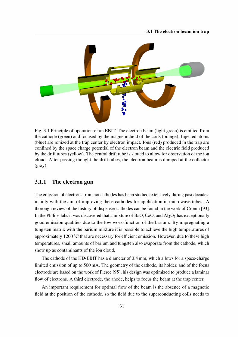
Fig. 3.1 Principle of operation of an EBIT. The electron beam (light green) is emitted fromthe cathode (green) and focused by the magnetic field of the coils (orange). Injected atoms(blue) are ionized at the trap center by electron impact. Ions (red) produced in the trap areconfined by the space charge potential of the electron beam and the electric field producedby the drift tubes (yellow). The central drift tube is slotted to allow for observation of the ioncloud. After passing thought the drift tubes, the electron beam is dumped at the collector(gray).
3.1.1 The electron gun
The emission of electrons from hot cathodes has been studied extensively during past decades;mainly with the aim of improving these cathodes for application in microwave tubes. Athorough review of the history of dispenser cathodes can be found in the work of Cronin [93].In the Philips labs it was discovered that a mixture of BaO, CaO, and Al2O3 has exceptionallygood emission qualities due to the low work-function of the barium. By impregnating atungsten matrix with the barium mixture it is possible to achieve the high temperatures ofapproximately 1200 C that are necessary for efficient emission. However, due to these hightemperatures, small amounts of barium and tungsten also evaporate from the cathode, whichshow up as contaminants of the ion cloud.
The cathode of the HD-EBIT has a diameter of 3.4 mm, which allows for a space-chargelimited emission of up to 500 mA. The geometry of the cathode, its holder, and of the focuselectrode are based on the work of Pierce [95], his design was optimized to produce a laminarflow of electrons. A third electrode, the anode, helps to focus the beam at the trap center.
An important requirement for optimal flow of the beam is the absence of a magneticfield at the position of the cathode, so the field due to the superconducting coils needs to
31

Experimental setup
Isolator Focus Cathode Anode
Heatsink Buckingcoil
Soft ironyoke
Fig. 3.2 Cross section of the electron gun of the HD-EBIT. The cathode, anode, and focuselectrode are mounted on the isolator, which is made of non-conductive Macor™. Theelectrical connections for the electrodes run through the isolator and connect to the flangeon the left (connections not shown). Cooling water flows through the heat sink to transportaway the heat produced in the bucking coil.
32
3.1 The electron beam ion trap
4 4 0 4 5 0 4 6 0 4 7 0 4 8 0 4 9 0 5 0 0 5 1 0 5 2 0 5 3 0 5 4 0 5 5 0 5 6 0 5 7 0 5 8 00 . 0
0 . 1
0 . 2
0 . 3
0 . 4
0 . 5
0 . 6
0 . 7
0 . 8
0 . 9
1 . 0
1 . 1
Mag
netic
fiel
d st
reng
th (T
)
P o s i t i o n ( m m )
4 0 0 5 0 0 6 0 0 7 0 0 8 0 00
1
2
3
4
5
6
7
8
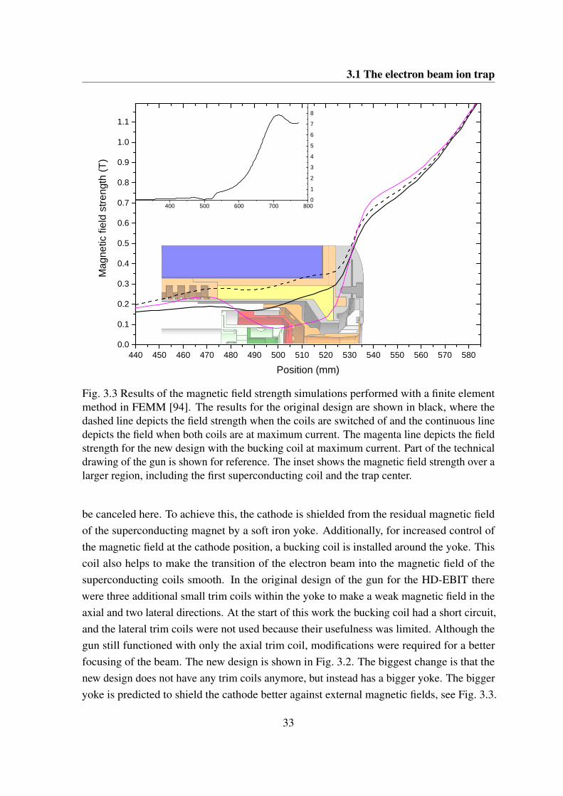
Fig. 3.3 Results of the magnetic field strength simulations performed with a finite elementmethod in FEMM [94]. The results for the original design are shown in black, where thedashed line depicts the field strength when the coils are switched of and the continuous linedepicts the field when both coils are at maximum current. The magenta line depicts the fieldstrength for the new design with the bucking coil at maximum current. Part of the technicaldrawing of the gun is shown for reference. The inset shows the magnetic field strength over alarger region, including the first superconducting coil and the trap center.
be canceled here. To achieve this, the cathode is shielded from the residual magnetic fieldof the superconducting magnet by a soft iron yoke. Additionally, for increased control ofthe magnetic field at the cathode position, a bucking coil is installed around the yoke. Thiscoil also helps to make the transition of the electron beam into the magnetic field of thesuperconducting coils smooth. In the original design of the gun for the HD-EBIT therewere three additional small trim coils within the yoke to make a weak magnetic field in theaxial and two lateral directions. At the start of this work the bucking coil had a short circuit,and the lateral trim coils were not used because their usefulness was limited. Although thegun still functioned with only the axial trim coil, modifications were required for a betterfocusing of the beam. The new design is shown in Fig. 3.2. The biggest change is that thenew design does not have any trim coils anymore, but instead has a bigger yoke. The biggeryoke is predicted to shield the cathode better against external magnetic fields, see Fig. 3.3.
33
Experimental setup
Two thermocouples were installed between the windings of the bucking coil. These are usedto monitor the temperature of the coil to prevent overheating and subsequent short circuits.Additional improvements were the increase of distance between the focus electrode and thehousing, thereby reducing the risk of discharges. The front of the gun housing was madesmoother to prevent discharges between the gun and electrodes directly in front of the gun.The new gun was installed in 2014 and performed very well. Currents of 400 mA at energiesof up to 60 keV were achieved, at which H-like Xe53+ was produced and extracted.
3.1.2 The central region
At the center of the EBIT the ions are produced and trapped. The central vacuum chamber ofthe HD-EBIT houses the drift tube assembly, the superconducting coils, and the cryogenicsystem, see 3.4. The superconducting coils of the HD-EBIT are mounted in a vessel whichholds enough liquid helium to keep the magnet immersed and in a superconducting statefor one week. This storage time is achieved due to two heat shields surrounding the liquidhelium vessel in the vacuum. With a cryocooler, the heat shields are cooled to 20 K and50 K. The large cryogenic surfaces provide pumping power in addition to the pumping withconventional turbomolecular pumps. In this manner a pressure of better than 10−10 mbar canbe achieved.
The drift tube assembly consists of nine electrodes and their support structure. It runsthrough two opposing ports of a six-way cross, with the central drift tube at the center of thecross. Following the drift tubes are two electrodes known as the trumpet and the transporttube. Potentials can be applied to these to adjust the guiding of electrons and ions to thecollector. The lower port of the six-way cross is employed for the injection of neutrals. Thetwo horizontal ports for measurements of the fluorescence light from the ion cloud. Accessto the upper arm was restricted so it was not used during this work.
3.1.3 The trap and the electron beam
The shape of the potential well at the central drift tube is mainly determined by the electronbeam radius. The Brillouin radius of the electron beam,
rB =
√meI
πε0veB2 , (3.1)
is only valid under the idealized conditions of a cathode temperature Tc = 0 K, and nomagnetic field Bc at the cathode. In equation (3.1), I is the current of the beam, v theaxial electron velocity, and B the magnetic field strength at the trap center. Under realistic
34

3.1 The electron beam ion trap
Fig. 3.4 Cross section of the central trapping region of the HD-EBIT. The electron beamtravels from left to right through the drift tubes that here are colored alternately yellow andred. The central six-way cross (blue) allows for observation of the ion cloud and injection ofparticles. The drift tubes are connected to power supplies via the vacuum feedthroughs at thetop right of the figure. The superconducting coils (orange) are mounted in the liquid heliumvessel that is surrounded by two cooled heat shields.
35
Experimental setup
conditions in an EBIT, Tc and Bc are not zero. The approximations of Herrmann [96] haveproven to realistically take this into account [97, 98]. It is defined as the radius of the cylindercontaining 80% of the electrons of the beam, and can be calculated by
rH = rB
√√√√12+
√14+
8mekBTcr2c
e2B2r4B
+B2
cr4c
B2r4B. (3.2)
The Herrmann radius is approximately 25 µm under the following conditions: Tc =1450 K,Bc = 0.10 T, B =8.00 T, cathode diameter rc =1.70 mm, I =40 mA, and electron beamenergy Ee =400 eV. These values are similar to the settings used for the measurementspresented in this work. The constants in equation (3.2) are the Boltzmann constant kB, theelectric constant ε0, the electron mass me, and the electron charge e. The radius of the ioncloud depends on the shape of the trapping potential as well as on parameters such as itscharge state distribution and temperature; radii up to 200 µm haven been observed [99, 100].
To estimate the radial potential in the trap the electron beam can be approximated by aninfinitely long tube with a homogeneous charge density
ρ =I
πvr2H. (3.3)
By employing Gauss his flux theorem and considering the boundary conditions the radialpotential is obtained by
φ(r) =ρ
2πε0ln(
rrDT9
)+UDT9, rH ≤ r ≤ rDT9 (3.4)
φ(r) =ρ
2πε0
(r2
2r2H− 1
2− ln
(r
rDT9
))+UDT9, r ≤ rH .
A derivation of this equation can be found for example in [101]. In Fig. 3.5 the radial potentialis shown for the parameters that were typically used during the iridium measurements. Oftenthe electron beam energy is estimated by
Ee = eUacc (3.5)
= e(−Uc +UDT9).
That is, the potential difference between the cathode and central drift tube. But as Fig. 3.5shows, the potential at the trap center is significantly changed by the space charge of theelectron beam itself. Additionally, the space charge of the ion cloud contributes to the total
36
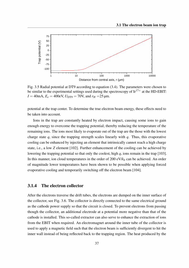
3.1 The electron beam ion trap
1 1 0 1 0 0 1 0 0 0 1 0 0 0 0
- 1 0 0
- 7 5
- 5 0
- 2 5
0
2 5
5 0
7 5Tr
ap p
oten
tial (
V)
D i s t a n c e f r o m c e n t r a l a x i s , r ( µm )
Fig. 3.5 Radial potential at DT9 according to equation (3.4). The parameters were chosen tobe similar to the experimental settings used during the spectroscopy of Ir17+ at the HD-EBIT:I = 40mA, Ee = 400eV, UDT9 = 70V, and rH =25 µm.
potential at the trap center. To determine the true electron beam energy, these effects need tobe taken into account.
Ions in the trap are constantly heated by electron impact, causing some ions to gainenough energy to overcome the trapping potential; thereby reducing the temperature of theremaining ions. The ions most likely to evaporate out of the trap are the those with the lowestcharge state q, since the trapping strength scales linearly with q. Thus, this evaporativecooling can be enhanced by injecting an element that intrinsically cannot reach a high chargestate, i.e., a low Z element [102]. Further enhancement of the cooling can be achieved bylowering the trapping potential so that only the coolest, high q, ions remain in the trap [103].In this manner, ion cloud temperatures in the order of 200 eV/kb can be achieved. An orderof magnitude lower temperatures have been shown to be possible when applying forcedevaporative cooling and temporarily switching off the electron beam [104].
3.1.4 The electron collector
After the electrons traverse the drift tubes, the electrons are dumped on the inner surface ofthe collector, see Fig. 3.6. The collector is directly connected to the same electrical groundas the cathode power supply so that the circuit is closed. To prevent electrons from passingthough the collector, an additional electrode at a potential more negative than that of thecathode is installed. This so-called extractor can also serve to enhance the extraction of ionsfrom the EBIT when required. An electromagnet around the inner tube of the collector isused to apply a magnetic field such that the electron beam is sufficiently divergent to hit theinner wall instead of being reflected back to the trapping region. The heat produced by the
37

Experimental setup
Inner tubeand heatsink
Collector coil
Extractor
Fig. 3.6 Cross section of the electron collector of the HD-EBIT. The electron beam (green)diverges strongly in the magnetic field of to the magnet coil (blue) and subsequently hits thewall of the inner tube (orange). The extractor (yellow) is biased to a sufficiently negativepotential to prevent the electrons from passing though the collector.
electrons hitting the collector, and the heat from the collector coil, is transported away bycooling water.
3.1.5 The injection system
In this work, the preferred method for injecting particles into the EBIT was by crossing amolecular beam with the electron beam at the trap center. Substances that are gaseous orvolatile at room temperature are most suited for this type of injection. For the injection of thechemical elements investigated in this work, suitable volatile compounds were found, seetable 3.1. The binding energies of molecules are at the level of a few eV, so their bonds areeasily broken by the electron beam. In addition to the elements of interest, the compoundsalso contain hydrogen, carbon, and oxygen. This is advantageous since the light elementsenhance evaporative cooling. At the HD-EBIT, a gas dosing valve was used to regulate theflow of gas into the first stage of the injection system, the pressure at this stage was typicallyin the 10−7 mbar range. The nozzle of the valve was aimed at a small aperture (a few mm2)that leads to the second injection stage, where the pressure is approximately an order ofmagnitude lower. The next aperture leads to the central trapping region. The nozzle of thevalve, both apertures, and the trap center are all in line to cross the molecular beam with theelectron beam.
38
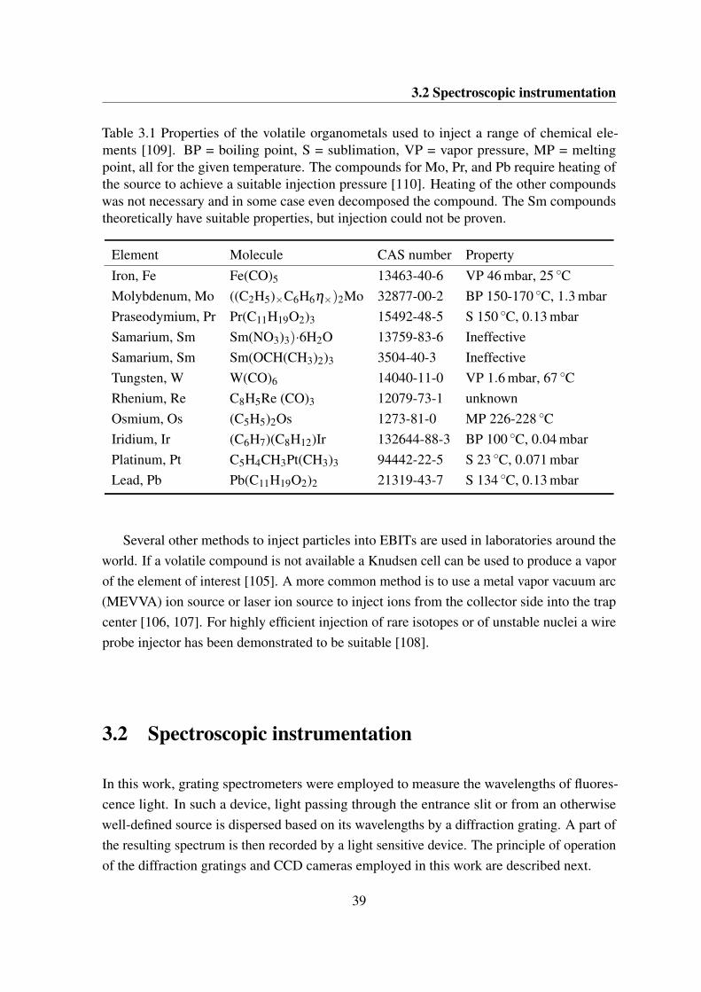
3.2 Spectroscopic instrumentation
Table 3.1 Properties of the volatile organometals used to inject a range of chemical ele-ments [109]. BP = boiling point, S = sublimation, VP = vapor pressure, MP = meltingpoint, all for the given temperature. The compounds for Mo, Pr, and Pb require heating ofthe source to achieve a suitable injection pressure [110]. Heating of the other compoundswas not necessary and in some case even decomposed the compound. The Sm compoundstheoretically have suitable properties, but injection could not be proven.
Element Molecule CAS number PropertyIron, Fe Fe(CO)5 13463-40-6 VP 46 mbar, 25 CMolybdenum, Mo ((C2H5)×C6H6η×)2Mo 32877-00-2 BP 150-170 C, 1.3 mbarPraseodymium, Pr Pr(C11H19O2)3 15492-48-5 S 150 C, 0.13 mbarSamarium, Sm Sm(NO3)3)·6H2O 13759-83-6 IneffectiveSamarium, Sm Sm(OCH(CH3)2)3 3504-40-3 IneffectiveTungsten, W W(CO)6 14040-11-0 VP 1.6 mbar, 67 CRhenium, Re C8H5Re (CO)3 12079-73-1 unknownOsmium, Os (C5H5)2Os 1273-81-0 MP 226-228 CIridium, Ir (C6H7)(C8H12)Ir 132644-88-3 BP 100 C, 0.04 mbarPlatinum, Pt C5H4CH3Pt(CH3)3 94442-22-5 S 23 C, 0.071 mbarLead, Pb Pb(C11H19O2)2 21319-43-7 S 134 C, 0.13 mbar
Several other methods to inject particles into EBITs are used in laboratories around theworld. If a volatile compound is not available a Knudsen cell can be used to produce a vaporof the element of interest [105]. A more common method is to use a metal vapor vacuum arc(MEVVA) ion source or laser ion source to inject ions from the collector side into the trapcenter [106, 107]. For highly efficient injection of rare isotopes or of unstable nuclei a wireprobe injector has been demonstrated to be suitable [108].
3.2 Spectroscopic instrumentation
In this work, grating spectrometers were employed to measure the wavelengths of fluores-cence light. In such a device, light passing through the entrance slit or from an otherwisewell-defined source is dispersed based on its wavelengths by a diffraction grating. A part ofthe resulting spectrum is then recorded by a light sensitive device. The principle of operationof the diffraction gratings and CCD cameras employed in this work are described next.
39
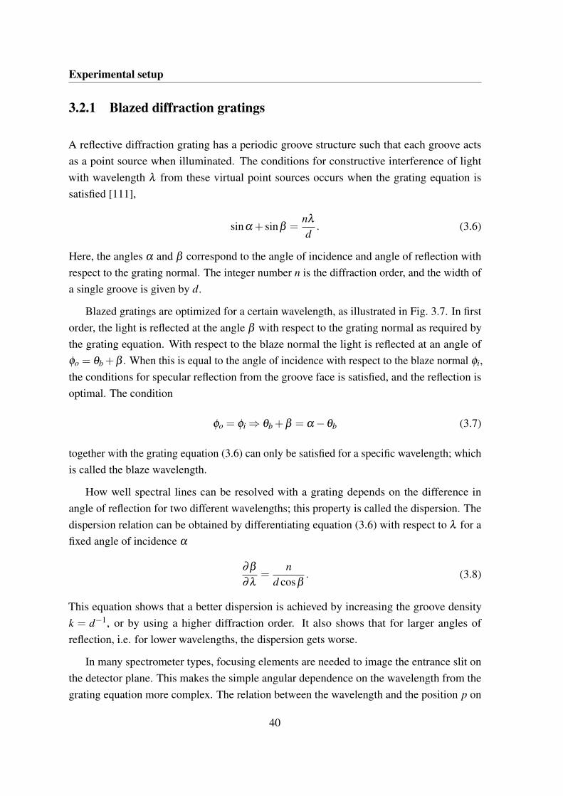
Experimental setup
3.2.1 Blazed diffraction gratings
A reflective diffraction grating has a periodic groove structure such that each groove actsas a point source when illuminated. The conditions for constructive interference of lightwith wavelength λ from these virtual point sources occurs when the grating equation issatisfied [111],
sinα + sinβ =nλ
d. (3.6)
Here, the angles α and β correspond to the angle of incidence and angle of reflection withrespect to the grating normal. The integer number n is the diffraction order, and the width ofa single groove is given by d.
Blazed gratings are optimized for a certain wavelength, as illustrated in Fig. 3.7. In firstorder, the light is reflected at the angle β with respect to the grating normal as required bythe grating equation. With respect to the blaze normal the light is reflected at an angle ofφo = θb +β . When this is equal to the angle of incidence with respect to the blaze normal φi,the conditions for specular reflection from the groove face is satisfied, and the reflection isoptimal. The condition
φo = φi ⇒ θb +β = α −θb (3.7)
together with the grating equation (3.6) can only be satisfied for a specific wavelength; whichis called the blaze wavelength.
How well spectral lines can be resolved with a grating depends on the difference inangle of reflection for two different wavelengths; this property is called the dispersion. Thedispersion relation can be obtained by differentiating equation (3.6) with respect to λ for afixed angle of incidence α
∂β
∂λ=
nd cosβ
. (3.8)
This equation shows that a better dispersion is achieved by increasing the groove densityk = d−1, or by using a higher diffraction order. It also shows that for larger angles ofreflection, i.e. for lower wavelengths, the dispersion gets worse.
In many spectrometer types, focusing elements are needed to image the entrance slit onthe detector plane. This makes the simple angular dependence on the wavelength from thegrating equation more complex. The relation between the wavelength and the position p on
40
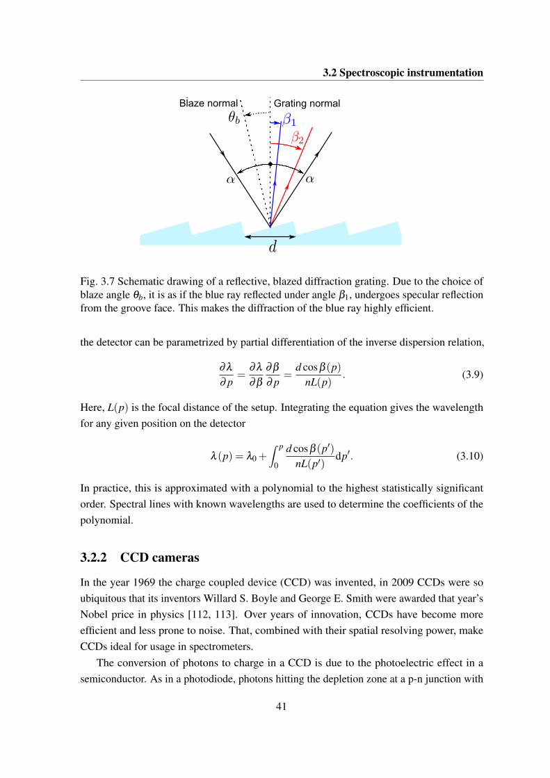
3.2 Spectroscopic instrumentation
Blaze normal Grating normal
Fig. 3.7 Schematic drawing of a reflective, blazed diffraction grating. Due to the choice ofblaze angle θb, it is as if the blue ray reflected under angle β1, undergoes specular reflectionfrom the groove face. This makes the diffraction of the blue ray highly efficient.
the detector can be parametrized by partial differentiation of the inverse dispersion relation,
∂λ
∂ p=
∂λ
∂β
∂β
∂ p=
d cosβ (p)nL(p)
. (3.9)
Here, L(p) is the focal distance of the setup. Integrating the equation gives the wavelengthfor any given position on the detector
λ (p) = λ0 +∫ p
0
d cosβ (p′)nL(p′)
dp′. (3.10)
In practice, this is approximated with a polynomial to the highest statistically significantorder. Spectral lines with known wavelengths are used to determine the coefficients of thepolynomial.
3.2.2 CCD cameras
In the year 1969 the charge coupled device (CCD) was invented, in 2009 CCDs were soubiquitous that its inventors Willard S. Boyle and George E. Smith were awarded that year’sNobel price in physics [112, 113]. Over years of innovation, CCDs have become moreefficient and less prone to noise. That, combined with their spatial resolving power, makeCCDs ideal for usage in spectrometers.
The conversion of photons to charge in a CCD is due to the photoelectric effect in asemiconductor. As in a photodiode, photons hitting the depletion zone at a p-n junction with
41
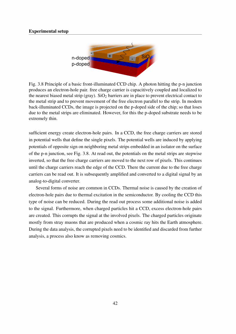
Experimental setup
+-
- SiO2n-dopedp-doped
Fig. 3.8 Principle of a basic front-illuminated CCD chip. A photon hitting the p-n junctionproduces an electron-hole pair. free charge carrier is capacitively coupled and localized tothe nearest biased metal strip (gray). SiO2 barriers are in place to prevent electrical contact tothe metal strip and to prevent movement of the free electron parallel to the strip. In modernback-illuminated CCDs, the image is projected on the p-doped side of the chip; so that losesdue to the metal strips are eliminated. However, for this the p-doped substrate needs to beextremely thin.
sufficient energy create electron-hole pairs. In a CCD, the free charge carriers are storedin potential wells that define the single pixels. The potential wells are induced by applyingpotentials of opposite sign on neighboring metal strips embedded in an isolator on the surfaceof the p-n junction, see Fig. 3.8. At read out, the potentials on the metal strips are stepwiseinverted, so that the free charge carriers are moved to the next row of pixels. This continuesuntil the charge carriers reach the edge of the CCD. There the current due to the free chargecarriers can be read out. It is subsequently amplified and converted to a digital signal by ananalog-to-digital converter.
Several forms of noise are common in CCDs. Thermal noise is caused by the creation ofelectron-hole pairs due to thermal excitation in the semiconductor. By cooling the CCD thistype of noise can be reduced. During the read out process some additional noise is addedto the signal. Furthermore, when charged particles hit a CCD, excess electron-hole pairsare created. This corrupts the signal at the involved pixels. The charged particles originatemostly from stray muons that are produced when a cosmic ray hits the Earth atmosphere.During the data analysis, the corrupted pixels need to be identified and discarded from furtheranalysis, a process also know as removing cosmics.
42
Chapter 4
Spectroscopy of Pm-like and Nd-likesystems in the extreme ultra-violetregime
The clearest way into the Universe is through a forest wilderness.
— John Muir
The elements in the alkali group of the periodic table have been subject to extensivestudy because of their relatively simple electronic structure with a single ns electron outsideclosed shells. For the same reason, singly charged ions of the alkaline earth metals are themain subject of many experiments in atomic physics. In the realm of highly charged ions(HCI) too there is considerable interest in alkali-like ions. For example, the 2s - 2p transitionin Li-like Pr56+ was recently studied as a means to access nuclear properties through thelevel splittings induced by the nuclear magnetic field [43]. Also, the transitions in Li-likeions have been extensively studied for their quantum electrodynamic (QED) contributions,see for example Epp et al. [63] and references therein. The 3s - 3p transitions of a widerange of Na-like ions were investigated in the work of Gillapsy et al. [44]. The reorderingof levels due to the dominance of the Coulomb interaction in HCI gives Ni-like ions with28 bound electrons a closed shell configuration. Hence, the next alkali-like series for HCIis the Cu-like sequence. Corresponding 4s - 4p transitions were investigated for a range ofions by Gillapsy et al. among other groups [44]. The 4 f –5s level crossing gives HCI of thePm-like (Z = 61) iso-electronic sequence configurations with a single 5s electron above aclosed n = 4 shell. Curtis and Ellis were the first to publish on their theoretical investigationof Pm-like HCI [46].
43
Spectroscopy of Pm-like and Nd-like systems in the extreme ultra-violet regime
Initially, it was suggested that the 5s 2S1/2 - 5p 2P1/2 and 5s 2S1/2 - 5p 2P3/2 doubletcould be used for diagnostic purposes of plasmas. Many nuclear fusion research facilitiesemploy divertors and other plasma facing components made of tungsten, causing smallamounts of sputtered tungsten to leak into the plasma. Current examples are ITER andWendelstein 7-X [114, 115]. From the observation of the 5s - 5p transitions of Pm-like W13+
in the plasma, properties such as the plasma temperature, amount of contamination, anddensity of the impurities can be deduced [116]. Controlling the impurities is important, sincetransitions of W in the x-ray region can radiate away significant amounts of energy [117, 118].
Since the publication by Curtis and Ellis much effort has been done to observe the 5s - 5ptransitions in a variety of Pm-like ions. A series of Pm-like ion species were studied using thebeam-foil technique at the Bochem Dynamitron-Tandem Laboratorium [119]. The heaviestPm-like ion investigated was U31+ at the TEXT tokamak, where the broad charge statedistribution made the interpretation of the spectra especially difficult [120]. At the ShanghaiEBIT, and more recently at the Tokyo-EBIT, the recorded spectra were less cluttered becausein EBITs the charge state distribution can be better tuned to a specific charge state [121, 79].Still, no definitive identification of 5s - 5p transitions was made due to the dense forest oflines. Tentative claims that were made are summarized in table 4.5 near the end of thischapter.
To interpret the dense spectra, it is necessary to turn to theory. On this front muchprogress has been made: Originally it was thought that in Pm-like W13+ the ground statewould be 5s 2S1/2. State-of-the-art calculations that are fully relativistic and take into accountmore configurations predict that only from Pm-like Pt17+ onward the 5s 2S1/2 configurationis the ground state [122, 123, 72]. This is illustrated in Fig. 4.1. The uncertainty of the latestpredictions is estimated to be at the level of 1% for the energy levels and at the level of 2% -20% for the transition rates.
Recent proposals to use HCI for metrology purposes sparked a renewed interest in,among others, the Pm-like systems [124]. The Nd-like ion Ir17+ is even more interestingfor fundamental research since it features transitions that are highly sensitive to variation ofthe fine-structure constant. Those transitions are in the optical range, which is covered inchapter 6. In order to interpret the complex electronic structure of Ir17+ the EUV spectraprovide essential information. They also provide additional data to benchmark atomic theoryfor atomic systems with complex correlations between many electrons in an open shell.
In this chapter, measurements of the EUV spectra of the Pm-like systems Re14+, Os15+,Ir16+, and Pt17+ are presented. The obtained spectra are compared to synthetic spectraproduced by a collisional radiative model (CRM) of the Flexible Atomic Code (FAC). Basedon this comparison, identifications of the lines was possible. The measured wavelengths
44
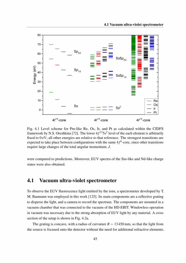
4.1 Vacuum ultra-violet spectrometer
Fig. 4.1 Level scheme for Pm-like Re, Os, Ir, and Pt as calculated within the CIDFSframework by N.S. Oreshkina [72]. The lower 4 f 135s2 level of the each element is arbitrarilyfixed to 0 eV; all other energies are relative to that reference. The strongest transitions areexpected to take place between configurations with the same 4 f k-core, since other transitionsrequire large changes of the total angular momentum, J.
were compared to predictions. Moreover, EUV spectra of the Sm-like and Nd-like chargestates were also obtained.
4.1 Vacuum ultra-violet spectrometer
To observe the EUV fluorescence light emitted by the ions, a spectrometer developed by T.M. Baumann was employed in this work [125]. Its main components are a reflective gratingto disperse the light, and a camera to record the spectrum. The components are mounted in avacuum chamber that was connected to the vacuum of the HD-EBIT. Windowless operationin vacuum was necessary due to the strong absorption of EUV light by any material. A crosssection of the setup is shown in Fig. 4.2a.
The grating is concave, with a radius of curvature R = 13450 mm, so that the light fromthe source is focused onto the detector without the need for additional refractive elements.
45
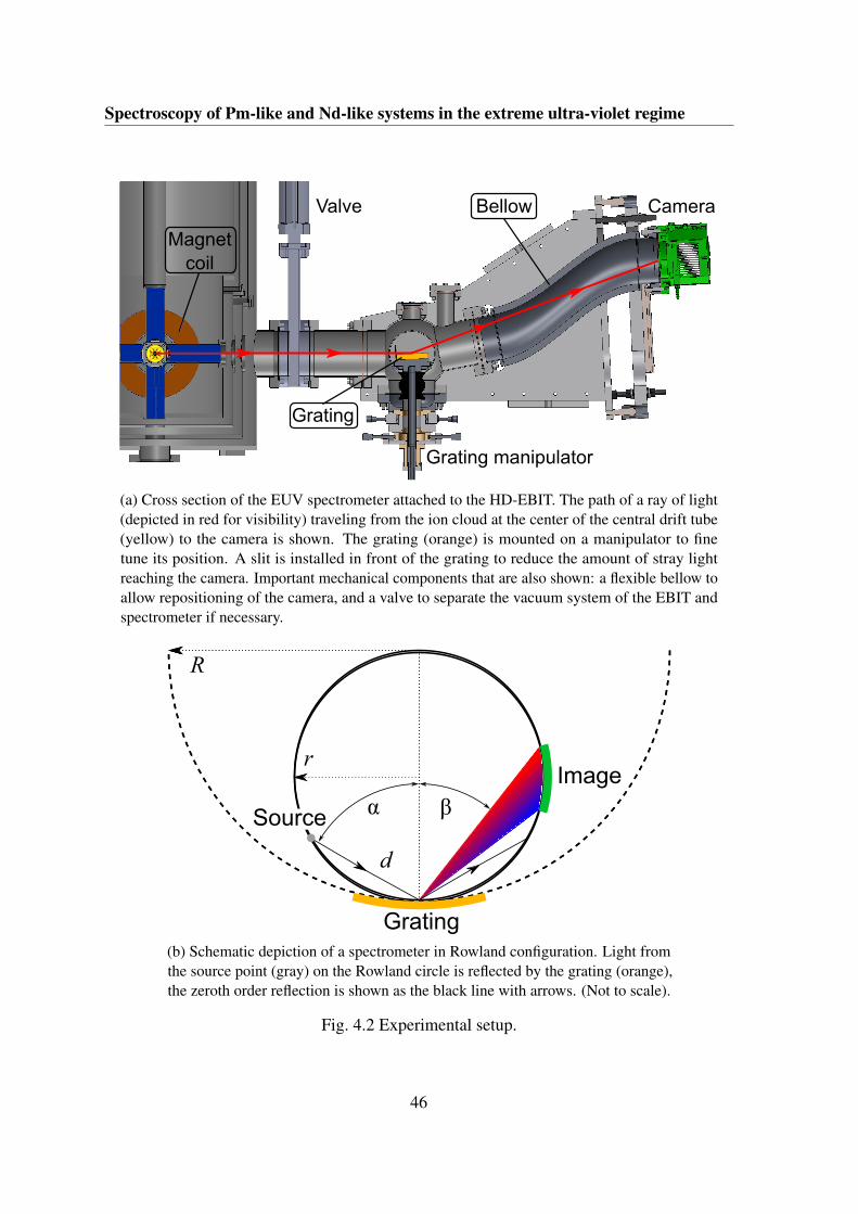
Spectroscopy of Pm-like and Nd-like systems in the extreme ultra-violet regime
Grating manipulator
CameraBellowValve
Magnetcoil
Grating
(a) Cross section of the EUV spectrometer attached to the HD-EBIT. The path of a ray of light(depicted in red for visibility) traveling from the ion cloud at the center of the central drift tube(yellow) to the camera is shown. The grating (orange) is mounted on a manipulator to finetune its position. A slit is installed in front of the grating to reduce the amount of stray lightreaching the camera. Important mechanical components that are also shown: a flexible bellow toallow repositioning of the camera, and a valve to separate the vacuum system of the EBIT andspectrometer if necessary.
R
r
Source
Image
Grating
α β
d
(b) Schematic depiction of a spectrometer in Rowland configuration. Light fromthe source point (gray) on the Rowland circle is reflected by the grating (orange),the zeroth order reflection is shown as the black line with arrows. (Not to scale).
Fig. 4.2 Experimental setup.
46
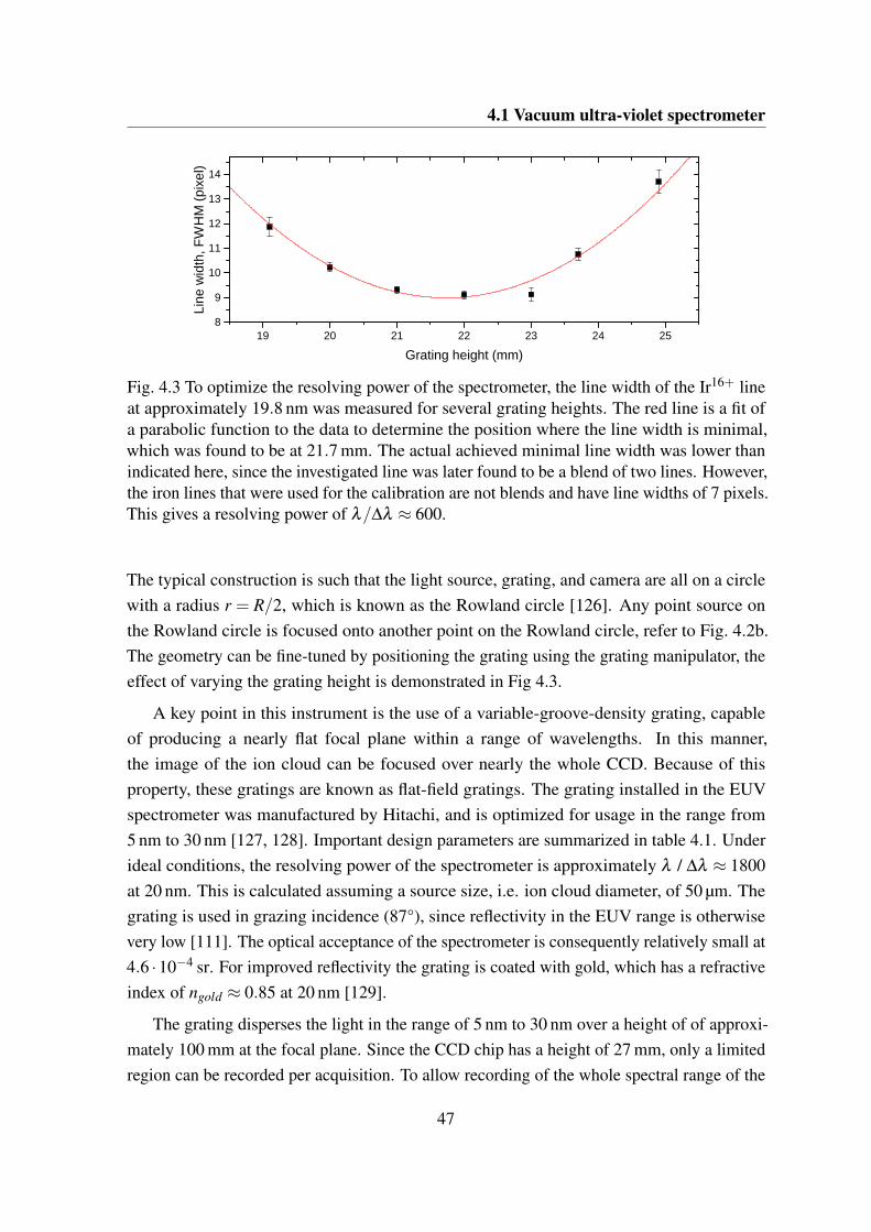
4.1 Vacuum ultra-violet spectrometer
1 9 2 0 2 1 2 2 2 3 2 4 2 58
9
1 0
1 1
1 2
1 3
1 4
Line
wid
th, F
WH
M (p
ixel
)
G r a t i n g h e i g h t ( m m )
Fig. 4.3 To optimize the resolving power of the spectrometer, the line width of the Ir16+ lineat approximately 19.8 nm was measured for several grating heights. The red line is a fit ofa parabolic function to the data to determine the position where the line width is minimal,which was found to be at 21.7 mm. The actual achieved minimal line width was lower thanindicated here, since the investigated line was later found to be a blend of two lines. However,the iron lines that were used for the calibration are not blends and have line widths of 7 pixels.This gives a resolving power of λ/∆λ ≈ 600.
The typical construction is such that the light source, grating, and camera are all on a circlewith a radius r = R/2, which is known as the Rowland circle [126]. Any point source onthe Rowland circle is focused onto another point on the Rowland circle, refer to Fig. 4.2b.The geometry can be fine-tuned by positioning the grating using the grating manipulator, theeffect of varying the grating height is demonstrated in Fig 4.3.
A key point in this instrument is the use of a variable-groove-density grating, capableof producing a nearly flat focal plane within a range of wavelengths. In this manner,the image of the ion cloud can be focused over nearly the whole CCD. Because of thisproperty, these gratings are known as flat-field gratings. The grating installed in the EUVspectrometer was manufactured by Hitachi, and is optimized for usage in the range from5 nm to 30 nm [127, 128]. Important design parameters are summarized in table 4.1. Underideal conditions, the resolving power of the spectrometer is approximately λ / ∆λ ≈ 1800at 20 nm. This is calculated assuming a source size, i.e. ion cloud diameter, of 50 µm. Thegrating is used in grazing incidence (87°), since reflectivity in the EUV range is otherwisevery low [111]. The optical acceptance of the spectrometer is consequently relatively small at4.6 ·10−4 sr. For improved reflectivity the grating is coated with gold, which has a refractiveindex of ngold ≈ 0.85 at 20 nm [129].
The grating disperses the light in the range of 5 nm to 30 nm over a height of of approxi-mately 100 mm at the focal plane. Since the CCD chip has a height of 27 mm, only a limitedregion can be recorded per acquisition. To allow recording of the whole spectral range of the
47
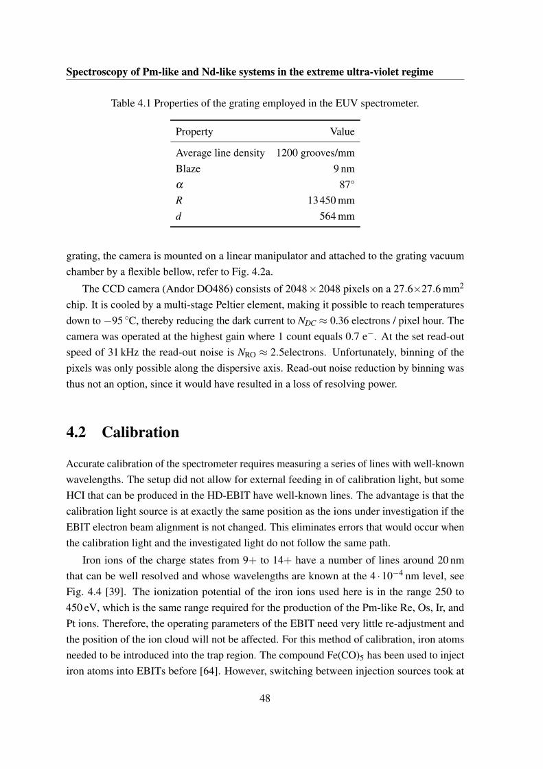
Spectroscopy of Pm-like and Nd-like systems in the extreme ultra-violet regime
Table 4.1 Properties of the grating employed in the EUV spectrometer.
Property Value
Average line density 1200 grooves/mmBlaze 9 nmα 87°R 13450 mmd 564 mm
grating, the camera is mounted on a linear manipulator and attached to the grating vacuumchamber by a flexible bellow, refer to Fig. 4.2a.
The CCD camera (Andor DO486) consists of 2048×2048 pixels on a 27.6×27.6 mm2
chip. It is cooled by a multi-stage Peltier element, making it possible to reach temperaturesdown to −95 C, thereby reducing the dark current to NDC ≈ 0.36 electrons / pixel hour. Thecamera was operated at the highest gain where 1 count equals 0.7 e−. At the set read-outspeed of 31 kHz the read-out noise is NRO ≈ 2.5electrons. Unfortunately, binning of thepixels was only possible along the dispersive axis. Read-out noise reduction by binning wasthus not an option, since it would have resulted in a loss of resolving power.
4.2 Calibration
Accurate calibration of the spectrometer requires measuring a series of lines with well-knownwavelengths. The setup did not allow for external feeding in of calibration light, but someHCI that can be produced in the HD-EBIT have well-known lines. The advantage is that thecalibration light source is at exactly the same position as the ions under investigation if theEBIT electron beam alignment is not changed. This eliminates errors that would occur whenthe calibration light and the investigated light do not follow the same path.
Iron ions of the charge states from 9+ to 14+ have a number of lines around 20 nmthat can be well resolved and whose wavelengths are known at the 4 ·10−4 nm level, seeFig. 4.4 [39]. The ionization potential of the iron ions used here is in the range 250 to450 eV, which is the same range required for the production of the Pm-like Re, Os, Ir, andPt ions. Therefore, the operating parameters of the EBIT need very little re-adjustment andthe position of the ion cloud will not be affected. For this method of calibration, iron atomsneeded to be introduced into the trap region. The compound Fe(CO)5 has been used to injectiron atoms into EBITs before [64]. However, switching between injection sources took at
48
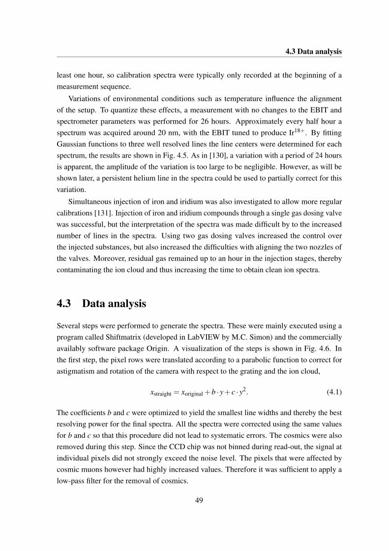
4.3 Data analysis
least one hour, so calibration spectra were typically only recorded at the beginning of ameasurement sequence.
Variations of environmental conditions such as temperature influence the alignmentof the setup. To quantize these effects, a measurement with no changes to the EBIT andspectrometer parameters was performed for 26 hours. Approximately every half hour aspectrum was acquired around 20 nm, with the EBIT tuned to produce Ir18+. By fittingGaussian functions to three well resolved lines the line centers were determined for eachspectrum, the results are shown in Fig. 4.5. As in [130], a variation with a period of 24 hoursis apparent, the amplitude of the variation is too large to be negligible. However, as will beshown later, a persistent helium line in the spectra could be used to partially correct for thisvariation.
Simultaneous injection of iron and iridium was also investigated to allow more regularcalibrations [131]. Injection of iron and iridium compounds through a single gas dosing valvewas successful, but the interpretation of the spectra was made difficult by to the increasednumber of lines in the spectra. Using two gas dosing valves increased the control overthe injected substances, but also increased the difficulties with aligning the two nozzles ofthe valves. Moreover, residual gas remained up to an hour in the injection stages, therebycontaminating the ion cloud and thus increasing the time to obtain clean ion spectra.
4.3 Data analysis
Several steps were performed to generate the spectra. These were mainly executed using aprogram called Shiftmatrix (developed in LabVIEW by M.C. Simon) and the commerciallyavailably software package Origin. A visualization of the steps is shown in Fig. 4.6. Inthe first step, the pixel rows were translated according to a parabolic function to correct forastigmatism and rotation of the camera with respect to the grating and the ion cloud,
xstraight = xoriginal +b · y+ c · y2. (4.1)
The coefficients b and c were optimized to yield the smallest line widths and thereby the bestresolving power for the final spectra. All the spectra were corrected using the same valuesfor b and c so that this procedure did not lead to systematic errors. The cosmics were alsoremoved during this step. Since the CCD chip was not binned during read-out, the signal atindividual pixels did not strongly exceed the noise level. The pixels that were affected bycosmic muons however had highly increased values. Therefore it was sufficient to apply alow-pass filter for the removal of cosmics.
49
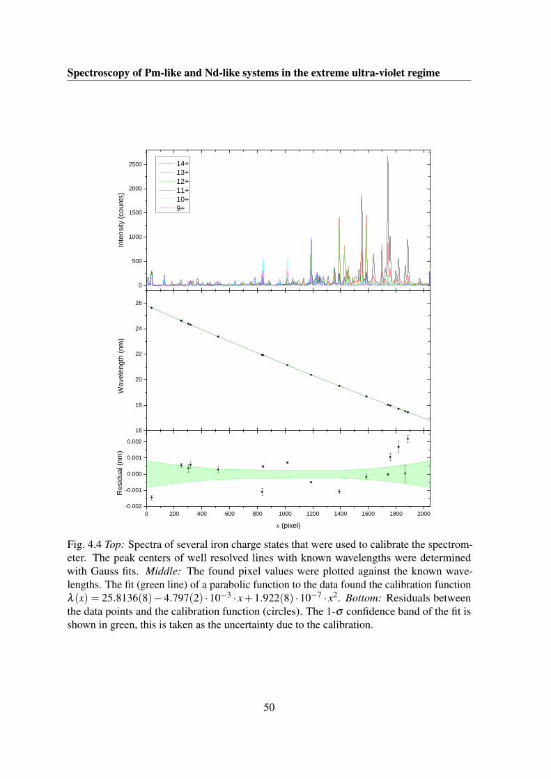
Spectroscopy of Pm-like and Nd-like systems in the extreme ultra-violet regime
0
5 0 0
1 0 0 0
1 5 0 0
2 0 0 0
2 5 0 0
1 6
1 8
2 0
2 2
2 4
2 6
0 2 0 0 4 0 0 6 0 0 8 0 0 1 0 0 0 1 2 0 0 1 4 0 0 1 6 0 0 1 8 0 0 2 0 0 0- 0 . 0 0 2
- 0 . 0 0 1
0 . 0 0 0
0 . 0 0 1
0 . 0 0 2
Inte
nsity
(cou
nts)
1 4 + 1 3 + 1 2 + 1 1 + 1 0 + 9 +
Wav
elen
gth
(nm
)R
esid
ual (
nm)
x ( p i x e l )
Fig. 4.4 Top: Spectra of several iron charge states that were used to calibrate the spectrom-eter. The peak centers of well resolved lines with known wavelengths were determinedwith Gauss fits. Middle: The found pixel values were plotted against the known wave-lengths. The fit (green line) of a parabolic function to the data found the calibration functionλ (x) = 25.8136(8)−4.797(2) ·10−3 · x+1.922(8) ·10−7 · x2. Bottom: Residuals betweenthe data points and the calibration function (circles). The 1-σ confidence band of the fit isshown in green, this is taken as the uncertainty due to the calibration.
50
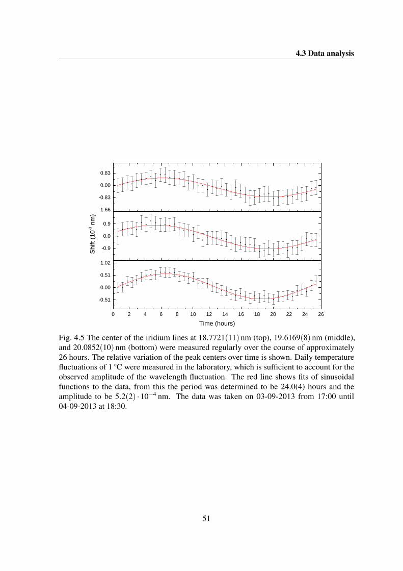
4.3 Data analysis
0 2 4 6 8 1 0 1 2 1 4 1 6 1 8 2 0 2 2 2 4 2 6
- 0 . 5 1
0 . 0 0
0 . 5 1
1 . 0 2
- 0 . 9
0 . 0
0 . 9
- 1 . 6 6
- 0 . 8 3
0 . 0 0
0 . 8 3
T i m e ( h o u r s )
Shi
ft (1
0-3 n
m)
Fig. 4.5 The center of the iridium lines at 18.7721(11) nm (top), 19.6169(8) nm (middle),and 20.0852(10) nm (bottom) were measured regularly over the course of approximately26 hours. The relative variation of the peak centers over time is shown. Daily temperaturefluctuations of 1 C were measured in the laboratory, which is sufficient to account for theobserved amplitude of the wavelength fluctuation. The red line shows fits of sinusoidalfunctions to the data, from this the period was determined to be 24.0(4) hours and theamplitude to be 5.2(2) ·10−4 nm. The data was taken on 03-09-2013 from 17:00 until04-09-2013 at 18:30.
51

Spectroscopy of Pm-like and Nd-like systems in the extreme ultra-violet regime
1660 1680 1700 1720 1740xoriginal (pixel)
0
500
1000
1500
2000
y (p
ixel)
(a) Zoom of raw CCD image
1660 1680 1700 1720 1740xstraight (pixel)
0
500
1000
1500
2000
y (p
ixel)
4950
5000
5050
5100
5150
5200
5250
5300
5350
5400
5450
Inte
nsi
ty (
counts
)
(b) Straightened and cleaned CCD image
500 1000 1500 2000
xstraight (pixel)
4950
5000
5050
5100
5150
5200
5250
5300
Inte
nsi
ty (
counts
)
(c) Projection
500 1000 1500 2000
xstraight (pixel)
0
20
40
60
80
100
120
140
Inte
nsi
ty (
counts
)
(d) Projection without background
Fig. 4.6 Step by step example of the data analysis procedure. In the first step the raw data (a)was transformed so that the spectral lines are straight and the cosmics are removed, resultingin (b). The 2D image was then projected onto the x-axis to produce the spectrum (c). Toproduce the final spectrum (d) the background was subtracted.
52
4.4 EUV spectra of Re, Os, Ir, and Pt
In the next step the image was projected onto the dispersive axis to produce a spectrum.Stray light from the electron gun cathode reaches the camera and produces a smooth but notflat background. This was measured by taking a spectrum while the trapping potential wasinverted, such that no ions remain trapped and only light due to other sources remains. Thisresults was then subtracted from the ion spectrum to produce the final results.
4.4 EUV spectra of Re, Os, Ir, and Pt
4.4.1 Full overview of the acquired data
At the Pm-like charge state of Re, Os, Ir, and Pt ions there are 61 remaining electrons boundto the nucleus. The ionization potentials of the Pm-like and neighboring charge states areseparated by maximally 50 eV, see table 4.3. Consequently, the charge state distributiondoes not strongly peak around one particular charge state. Hence, the spectra containedcontributions from several charge states. In order to clearly determine which charge stategenerates which line, it was necessary to vary the electron beam energy while monitoring theline intensities. Lines that show the same intensity behavior belong to the same charge state.
At the beginning of a measurement sequence, the electron beam energy was tuned to avalue well below the energy required for the production of the Pm-like charge state. The firstspectrum of the sequence was taken at these settings. Subsequently, the potential on all drifttubes was increased by 10 V and the next spectrum was taken. This procedure continueduntil the electron beam energy was well above the ionization energy of the Pm-like chargestate. At the end of the sequence, a spectrum of the background light was acquired. Anoverview of the results for Re, Os, Ir, and Pt can be seen in Fig. 4.7. Important experimentalparameters are listed in table 4.2. Iridium spectra were taken for the whole spectral rangefrom 5 to 30 nm [131]. However, beyond the region shown in Fig. 4.7, no strong lines werefound.
As expected, there are strong similarities between the spectra of ions belonging to thesame isoelectronic sequence. Characteristic lines appear at a slightly shifted wavelengths,that can be explained by the scaling with Z2 of the binding energies. Since in this workonly the spectra of the Pm-like and Nd-like sequence are of interest, those are the subject offurther studies in subsequent sections. At approximately 24.3 nm a line can be seen (mostnoticeable in the Re spectra) that does not show a variation of intensity over the range ofelectron beam energies. This line could be assigned to the He+ doublet 4p 2P1/2 - 1s 2S1/2
and 4p 2P3/2 - 1s 2S1/2 of which the wavelengths are known to be 24.302644454 nm and24.302687696 nm [132]. It was used where possible to correct for the spectrometer shifts
53
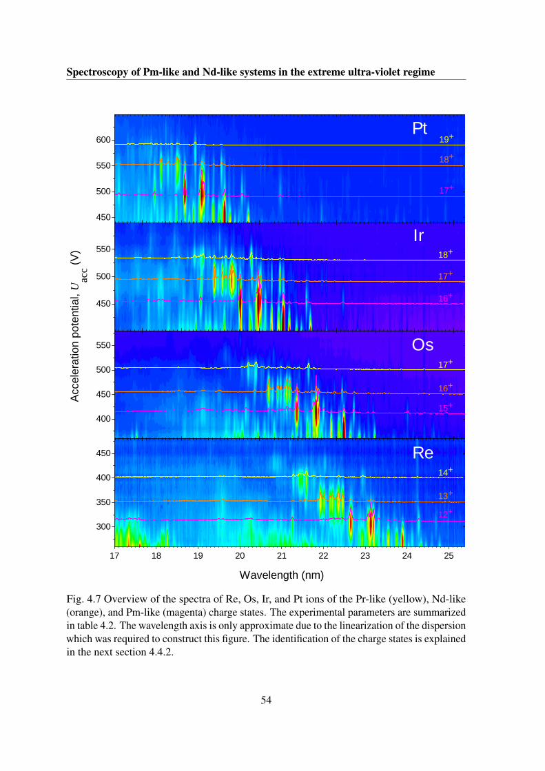
Spectroscopy of Pm-like and Nd-like systems in the extreme ultra-violet regime
4 5 0
5 0 0
5 5 0
6 0 0
1 3 +
1 6 +
1 7 +
1 8 +
1 4 +
1 7 +
1 8 +
P t
1 9 +
4 5 0
5 0 0
5 5 0
1 2 +
1 5 +
1 6 +
1 7 +
4 0 0
4 5 0
5 0 0
5 5 0
1 7 1 8 1 9 2 0 2 1 2 2 2 3 2 4 2 5
3 0 0
3 5 0
4 0 0
4 5 0
I r
O s
Acc
eler
atio
n po
tent
ial,
Uac
c (V)
W a v e l e n g t h ( n m )
R e
Fig. 4.7 Overview of the spectra of Re, Os, Ir, and Pt ions of the Pr-like (yellow), Nd-like(orange), and Pm-like (magenta) charge states. The experimental parameters are summarizedin table 4.2. The wavelength axis is only approximate due to the linearization of the dispersionwhich was required to construct this figure. The identification of the charge states is explainedin the next section 4.4.2.
54
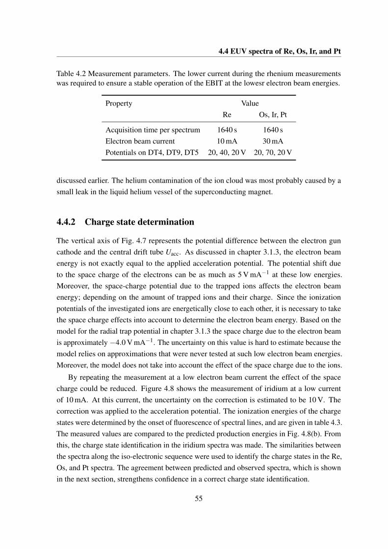
4.4 EUV spectra of Re, Os, Ir, and Pt
Table 4.2 Measurement parameters. The lower current during the rhenium measurementswas required to ensure a stable operation of the EBIT at the lowesr electron beam energies.
Property ValueRe Os, Ir, Pt
Acquisition time per spectrum 1640 s 1640 sElectron beam current 10 mA 30 mAPotentials on DT4, DT9, DT5 20, 40, 20 V 20, 70, 20 V
discussed earlier. The helium contamination of the ion cloud was most probably caused by asmall leak in the liquid helium vessel of the superconducting magnet.
4.4.2 Charge state determination
The vertical axis of Fig. 4.7 represents the potential difference between the electron guncathode and the central drift tube Uacc. As discussed in chapter 3.1.3, the electron beamenergy is not exactly equal to the applied acceleration potential. The potential shift dueto the space charge of the electrons can be as much as 5 V mA−1 at these low energies.Moreover, the space-charge potential due to the trapped ions affects the electron beamenergy; depending on the amount of trapped ions and their charge. Since the ionizationpotentials of the investigated ions are energetically close to each other, it is necessary to takethe space charge effects into account to determine the electron beam energy. Based on themodel for the radial trap potential in chapter 3.1.3 the space charge due to the electron beamis approximately −4.0 V mA−1. The uncertainty on this value is hard to estimate because themodel relies on approximations that were never tested at such low electron beam energies.Moreover, the model does not take into account the effect of the space charge due to the ions.
By repeating the measurement at a low electron beam current the effect of the spacecharge could be reduced. Figure 4.8 shows the measurement of iridium at a low currentof 10 mA. At this current, the uncertainty on the correction is estimated to be 10 V. Thecorrection was applied to the acceleration potential. The ionization energies of the chargestates were determined by the onset of fluorescence of spectral lines, and are given in table 4.3.The measured values are compared to the predicted production energies in Fig. 4.8(b). Fromthis, the charge state identification in the iridium spectra was made. The similarities betweenthe spectra along the iso-electronic sequence were used to identify the charge states in the Re,Os, and Pt spectra. The agreement between predicted and observed spectra, which is shownin the next section, strengthens confidence in a correct charge state identification.
55
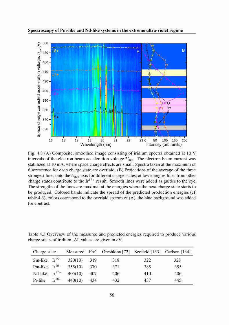
Spectroscopy of Pm-like and Nd-like systems in the extreme ultra-violet regime
0 5 0 1 0 0 1 5 0 2 0 01 6 1 7 1 8 1 9 2 0 2 1 2 2 2 3
3 2 0
3 4 0
3 6 0
3 8 0
4 0 0
4 2 0
4 4 0
4 6 0
4 8 0
5 0 0
1 5 +
1 6 +
1 7 +
A
W a v e l e n g t h ( n m )
Spa
ce c
harg
e co
rrect
ed a
ccel
erat
ion
volta
ge, U
acc (
V)
1 8 +
I n t e n s i t y ( a r b . u n i t s )
B
Fig. 4.8 (A) Composite, smoothed image consisting of iridium spectra obtained at 10 Vintervals of the electron beam acceleration voltage Uacc. The electron beam current wasstabilized at 10 mA, where space charge effects are small. Spectra taken at the maximum offluorescence for each charge state are overlaid. (B) Projections of the average of the threestrongest lines onto the Uacc-axis for different charge states; at low energies lines from othercharge states contribute to the Ir17+ result. Smooth lines were added as guides to the eye.The strengths of the lines are maximal at the energies where the next charge state starts tobe produced. Colored bands indicate the spread of the predicted production energies (cf.table 4.3); colors correspond to the overlaid spectra of (A), the blue background was addedfor contrast.
Table 4.3 Overview of the measured and predicted energies required to produce variouscharge states of iridium. All values are given in eV.
Charge state Measured FAC Oreshkina [72] Scofield [133] Carlson [134]
Sm-like Ir15+ 320(10) 319 318 322 328Pm-like Ir16+ 355(10) 370 371 385 355Nd-like Ir17+ 405(10) 407 406 410 406Pr-like Ir18+ 440(10) 434 432 437 445
56
4.5 Identifications of lines in the Pm-like spectra
4.5 Identifications of lines in the Pm-like spectra
The individual EUV spectra of Pm-like Re, Os, Ir, and Pt obtained in this work are shownin Fig 4.9. Gaussian functions were fitted to well-resolved lines that belonged to the Pm-like charge state to determine the central wavelength and peak intensity. The results aresummarized in table 4.4. The use of Gaussian functions to fit the lines was motivated by theexpected Doppler broadening and by the spatial distribution of the ion cloud. Furthermore, theZeeman splitting is expected to be at the order of 10−4 eV, which is too small to be resolvedwith the employed spectrometer. The quality of the fits was monitored by verifying that thereduced χ2 was satisfactory and by checking the fit residuals for deviations from the normaldistribution. The confidence in the correctness of the fits was supported by confirming thatthe found line widths correspond to the resolving power of the spectrometer as determinedwith the Fe lines. In some cases the width of a line was found to significantly exceed theexpected value. This can be caused by blended transitions with near equal transition energiesand strengths. Lines with increased widths are marked in the fit results table.
Ideally, predictions for the transition energies and rates are good enough to directlyidentify lines by comparing them to the predictions. Based on predictions such as presentedin Fig. 4.1, or as can be found in the work by M.S. Safronova et al. [124], a dense clusterof bright lines is to be expected in the investigated region of the Pm-like spectra. Similarpredictions for the atomic structure and transition rates were obtained with FAC calculations.A synthetic spectrum based on these results is shown in Fig 4.10a. According to theory, thestrongest transitions take place within the 4 f 12-core configurations. Transition rates are in theorder of 1011 s−1 for the strongest 4 f 125s5p2 to 4 f 125s25p transitions, whereas the 4 f 135p1
to 4 f 135s1 transitions are predicted to have a rate of approximately 1010 s−1. Clearly, theobserved spectra do not show the predicted large number of strong transitions. To explainthis, the excitation processes in the EBIT and the branching ratios of the decay channels needto be taken into account using CRM.
First, the energy levels, transition rates, and electron impact (de-)excitation cross sectionswere calculated for the 4 f 145(s, p,d), 4 f 135s2, 4 f 135s5p, 4 f 125s25(p,d), and 4 f 125s5p2
configurations. This set of eight configurations was chosen because it reproduced theobserved spectra the best. Inclusion of more configurations (up to twenty configurationsin total) shifted the transitions to higher energies. The calculated transition rates and crosssections were used in the CRM calculation to numerically solve the quasi-stationary-staterate equations. For this, an electron density of 1011 cm−3 was chosen, as explained in thenext section. The electron energy distribution was centered at 395 eV and set to follow aGaussian distribution with a width of 5 eV, the distribution was cut off at 390 eV and 400 eV.The solution gives the line strengths corrected for the energy level population distribution
57
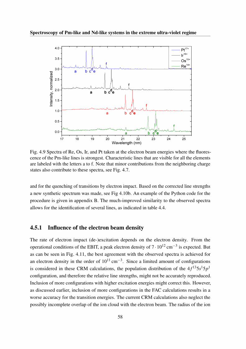
Spectroscopy of Pm-like and Nd-like systems in the extreme ultra-violet regime
Fig. 4.9 Spectra of Re, Os, Ir, and Pt taken at the electron beam energies where the fluores-cence of the Pm-like lines is strongest. Characteristic lines that are visible for all the elementsare labeled with the letters a to f. Note that minor contributions from the neighboring chargestates also contribute to these spectra, see Fig. 4.7.
and for the quenching of transitions by electron impact. Based on the corrected line strengthsa new synthetic spectrum was made, see Fig 4.10b. An example of the Python code for theprocedure is given in appendix B. The much-improved similarity to the observed spectraallows for the identification of several lines, as indicated in table 4.4.
4.5.1 Influence of the electron beam density
The rate of electron impact (de-)excitation depends on the electron density. From theoperational conditions of the EBIT, a peak electron density of 7 ·1012 cm−3 is expected. Butas can be seen in Fig. 4.11, the best agreement with the observed spectra is achieved foran electron density in the order of 1011 cm−3. Since a limited amount of configurationsis considered in these CRM calculations, the population distribution of the 4 f 135s15p1
configuration, and therefore the relative line strengths, might not be accurately reproduced.Inclusion of more configurations with higher excitation energies might correct this. However,as discussed earlier, inclusion of more configurations in the FAC calculations results in aworse accuracy for the transition energies. The current CRM calculations also neglect thepossibly incomplete overlap of the ion cloud with the electron beam. The radius of the ion
58
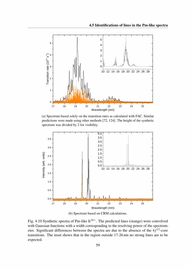
4.5 Identifications of lines in the Pm-like spectra
1 7 1 8 1 9 2 0 2 1 2 2 2 3 2 4 2 5
0
1
2
3
4
5
Tran
sitio
n ra
te (1
011 s
-1)
W a v e l e n g t h ( n m )
1 0 1 2 1 4 1 6 1 8 2 0 2 2 2 4 2 6 2 8
0
1
2
3
4
5
(a) Spectrum based solely on the transition rates as calculated with FAC. Similarpredictions were made using other methods [72, 124]. The height of the syntheticspectrum was divided by 2 for visibility.
1 7 1 8 1 9 2 0 2 1 2 2 2 3 2 4 2 5
0 . 0
0 . 5
1 . 0
1 . 5
2 . 0
2 . 5
3 . 0
3 . 5
Inte
nsity
(arb
. uni
ts)
W a v e l e n g t h ( n m )
1 0 1 2 1 4 1 6 1 8 2 0 2 2 2 4 2 6 2 80 . 00 . 51 . 01 . 52 . 02 . 53 . 03 . 54 . 0
(b) Spectrum based on CRM calculations.
Fig. 4.10 Synthetic spectra of Pm-like Ir16+. The predicted lines (orange) were convolvedwith Gaussian functions with a width corresponding to the resolving power of the spectrom-eter. Significant differences between the spectra are due to the absence of the 4 f 12-coretransitions. The inset shows that in the region outside 17-26 nm no strong lines are to beexpected.
59
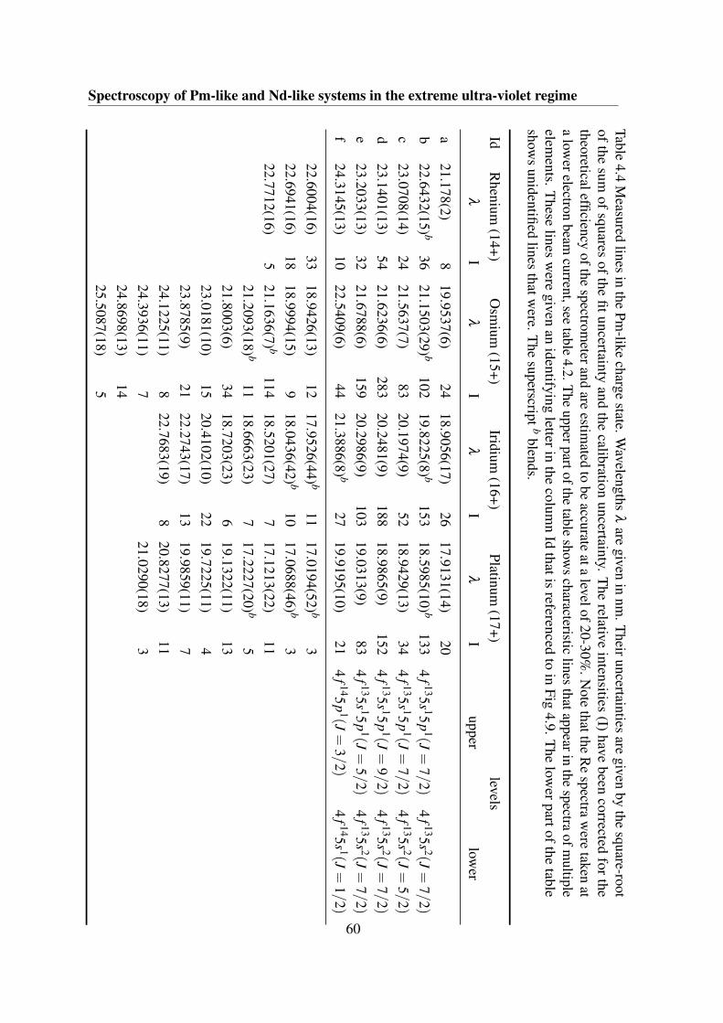
Spectroscopy of Pm-like and Nd-like systems in the extreme ultra-violet regimeTable
4.4M
easuredlines
inthe
Pm-like
chargestate.W
avelengthsλ
aregiven
innm
.Theiruncertainties
aregiven
bythe
square-rootof
thesum
ofsquares
ofthe
fituncertaintyand
thecalibration
uncertainty.T
herelative
intensities(I)
havebeen
correctedfor
thetheoreticalefficiency
ofthespectrom
eterandare
estimated
tobe
accurateata
levelof20-30%.N
otethatthe
Re
spectraw
eretaken
ata
lowerelectron
beamcurrent,see
table4.2.The
upperpartofthetable
shows
characteristiclines
thatappearinthe
spectraofm
ultipleelem
ents.These
linesw
eregiven
anidentifying
letterinthe
column
Idthatis
referencedto
inFig
4.9.The
lowerpartofthe
tableshow
sunidentified
linesthatw
ere.The
superscriptb
blends.
IdR
henium(14+)
Osm
ium(15+)
Iridium(16+)
Platinum(17+)
levelsλ
Iλ
Iλ
Iλ
Iupper
lower
a21.178(2)
819.9537(6)
2418.9056(17)
2617.9131(14)
20b
22.6432(15) b36
21.1503(29) b102
19.8225(8) b153
18.5985(10) b133
4f 135s 15p
1(J=
7/2
)4
f 135s 2(J=
7/2)
c23.0708(14)
2421.5637(7)
8320.1974(9)
5218.9429(13)
344
f 135s 15p1(J
=7/2
)4
f 135s 2(J=
5/2)
d23.1401(13)
5421.6236(6)
28320.2481(9)
18818.9865(9)
1524
f 135s 15p1(J
=9/2
)4
f 135s 2(J=
7/2)
e23.2033(13)
3221.6788(6)
15920.2986(9)
10319.0313(9)
834
f 135s 15p1(J
=5/2
)4
f 135s 2(J=
7/2)
f24.3145(13)
1022.5409(6)
4421.3886(8) b
2719.9195(10)
214
f 145p1(J
=3/2
)4
f 145s 1(J=
1/2
)
22.6004(16)33
18.9426(13)12
17.9526(44) b11
17.0194(52) b3
22.6941(16)18
18.9994(15)9
18.0436(42) b10
17.0688(46) b3
22.7712(16)5
21.1636(7) b114
18.5201(27)7
17.1213(22)11
21.2093(18) b11
18.6663(23)7
17.2227(20) b5
21.8003(6)34
18.7203(23)6
19.1322(11)13
23.0181(10)15
20.4102(10)22
19.7225(11)4
23.8785(9)21
22.2743(17)13
19.9859(11)7
24.1225(11)8
22.7683(19)8
20.8277(13)11
24.3936(11)7
21.0290(18)3
24.8698(13)14
25.5087(18)5
60
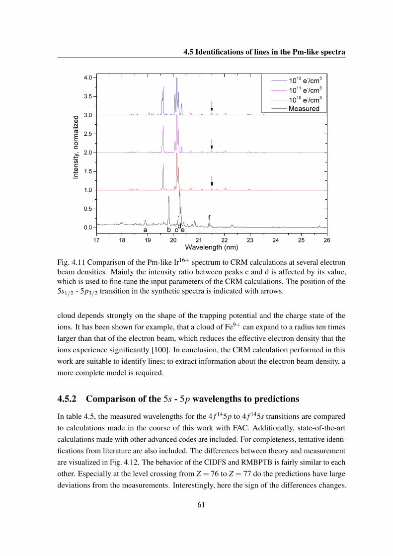
4.5 Identifications of lines in the Pm-like spectra
Fig. 4.11 Comparison of the Pm-like Ir16+ spectrum to CRM calculations at several electronbeam densities. Mainly the intensity ratio between peaks c and d is affected by its value,which is used to fine-tune the input parameters of the CRM calculations. The position of the5s1/2 - 5p3/2 transition in the synthetic spectra is indicated with arrows.
cloud depends strongly on the shape of the trapping potential and the charge state of theions. It has been shown for example, that a cloud of Fe9+ can expand to a radius ten timeslarger than that of the electron beam, which reduces the effective electron density that theions experience significantly [100]. In conclusion, the CRM calculation performed in thiswork are suitable to identify lines; to extract information about the electron beam density, amore complete model is required.
4.5.2 Comparison of the 5s - 5p wavelengths to predictions
In table 4.5, the measured wavelengths for the 4 f 145p to 4 f 145s transitions are comparedto calculations made in the course of this work with FAC. Additionally, state-of-the-artcalculations made with other advanced codes are included. For completeness, tentative identi-fications from literature are also included. The differences between theory and measurementare visualized in Fig. 4.12. The behavior of the CIDFS and RMBPTB is fairly similar to eachother. Especially at the level crossing from Z = 76 to Z = 77 do the predictions have largedeviations from the measurements. Interestingly, here the sign of the differences changes.
61
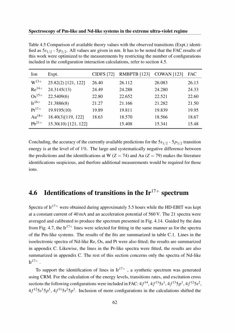
Spectroscopy of Pm-like and Nd-like systems in the extreme ultra-violet regime
Table 4.5 Comparison of available theory values with the observed transitions (Expt.) identi-fied as 5s1/2 - 5p3/2. All values are given in nm. It has to be noted that the FAC results ofthis work were optimized to the measurements by restricting the number of configurationsincluded in the configuration interaction calculations, refer to section 4.5.
Ion Expt. CIDFS [72] RMBPTB [123] COWAN [123] FAC
W13+ 25.82(2) [121, 122] 26.40 26.112 26.083 26.13Re14+ 24.3145(13) 24.49 24.288 24.280 24.33Os15+ 22.5409(6) 22.80 22.652 22.521 22.60Ir16+ 21.3886(8) 21.27 21.166 21.282 21.50Pt17+ 19.9195(10) 19.89 19.811 19.839 19.95Au18+ 18.40(3)[119, 122] 18.63 18.570 18.566 18.67Pb21+ 15.30(10) [121, 122] 15.408 15.341 15.48
Concluding, the accuracy of the currently available predictions for the 5s1/2 - 5p3/2 transitionenergy is at the level of of 1%. The large and systematically negative difference betweenthe predictions and the identifications at W (Z = 74) and Au (Z = 79) makes the literatureidentifications suspicious, and therfore additional measurements would be required for thoseions.
4.6 Identifications of transitions in the Ir17+ spectrum
Spectra of Ir17+ were obtained during approximately 5.5 hours while the HD-EBIT was keptat a constant current of 40 mA and an acceleration potential of 560 V. The 21 spectra wereaveraged and calibrated to produce the spectrum presented in Fig. 4.14. Guided by the datafrom Fig. 4.7, the Ir17+ lines were selected for fitting in the same manner as for the spectraof the Pm-like systems. The results of the fits are summarized in table C.1. Lines in theisoelectronic spectra of Nd-like Re, Os, and Pt were also fitted; the results are summarizedin appendix C. Likewise, the lines in the Pr-like spectra were fitted, the results are alsosummarized in appendix C. The rest of this section concerns only the spectra of Nd-likeIr17+ .
To support the identification of lines in Ir17+ , a synthetic spectrum was generatedusing CRM. For the calculation of the energy levels, transitions rates, and excitation crosssections the following configurations were included in FAC: 4 f 14, 4 f 135s1, 4 f 135p1, 4 f 125s2,4 f 125s15p1, 4 f 115s25p1. Inclusion of more configurations in the calculations shifted the
62
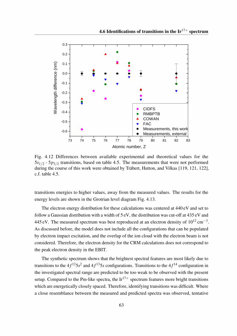
4.6 Identifications of transitions in the Ir17+ spectrum
7 3 7 4 7 5 7 6 7 7 7 8 7 9 8 0 8 1 8 2 8 3
- 0 . 6
- 0 . 5
- 0 . 4
- 0 . 3
- 0 . 2
- 0 . 1
0 . 0
0 . 1
0 . 2
0 . 3
Wav
elen
gth
diffe
renc
e (n
m)
A t o m i c n u m b e r , Z
C I D F S R M B P T B C O W A N F A C M e a s u r e m e n t s , t h i s w o r k M e a s u r e m e n t s , e x t e r n a l
Fig. 4.12 Differences between available experimental and theoretical values for the5s1/2 - 5p3/2 transitions, based on table 4.5. The measurements that were not performedduring the course of this work were obtained by Träbert, Hutton, and Vilkas [119, 121, 122],c.f. table 4.5.
transitions energies to higher values, away from the measured values. The results for theenergy levels are shown in the Grotrian level diagram Fig. 4.13.
The electron energy distribution for these calculations was centered at 440 eV and set tofollow a Gaussian distribution with a width of 5 eV, the distribution was cut-off at 435 eV and445 eV. The measured spectrum was best reproduced at an electron density of 1012 cm−3.As discussed before, the model does not include all the configurations that can be populatedby electron impact excitation, and the overlap of the ion cloud with the electron beam is notconsidered. Therefore, the electron density for the CRM calculations does not correspond tothe peak electron density in the EBIT.
The synthetic spectrum shows that the brightest spectral features are most likely due totransitions to the 4 f 125s2 and 4 f 135s configurations. Transitions to the 4 f 14 configuration inthe investigated spectral range are predicted to be too weak to be observed with the presentsetup. Compared to the Pm-like spectra, the Ir17+ spectrum features more bright transitionswhich are energetically closely spaced. Therefore, identifying transitions was difficult. Wherea close resemblance between the measured and predicted spectra was observed, tentative
63
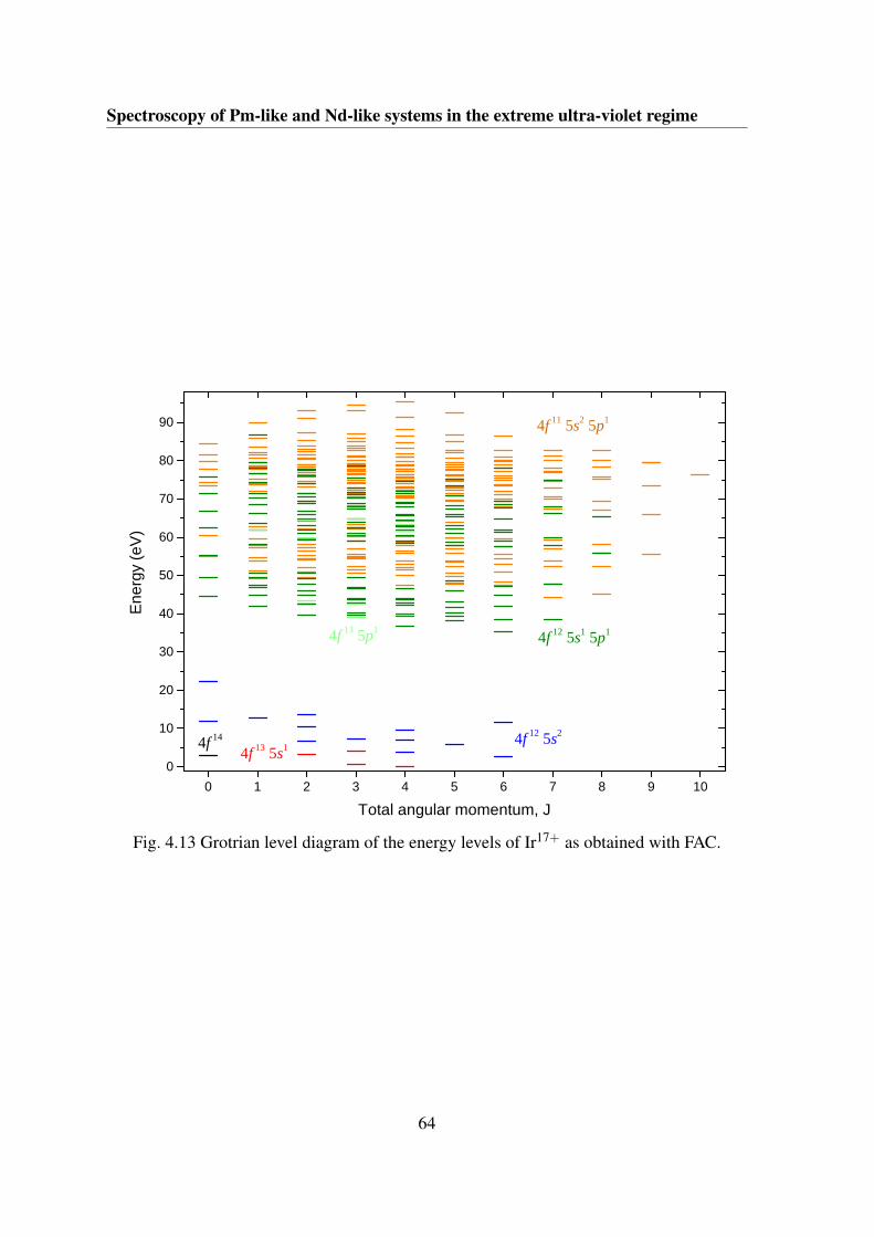
Spectroscopy of Pm-like and Nd-like systems in the extreme ultra-violet regime
0 1 2 3 4 5 6 7 8 9 1 00
1 0
2 0
3 0
4 0
5 0
6 0
7 0
8 0
9 0
4 f 1 3 5 p 1 4 f 1 2 5 s 1 5 p 1
4 f 1 1 5 s 2 5 p 1
4 f 1 3 5 s 14 f 1 4
Ene
rgy
(eV
)
T o t a l a n g u l a r m o m e n t u m , J
4 f 1 2 5 s 2
Fig. 4.13 Grotrian level diagram of the energy levels of Ir17+ as obtained with FAC.
64
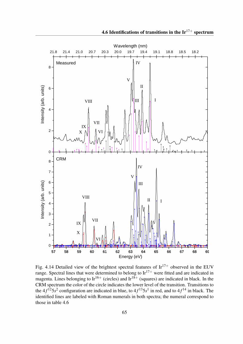
4.6 Identifications of transitions in the Ir17+ spectrum
2 1 . 8 2 1 . 4 2 1 . 0 2 0 . 7 2 0 . 3 2 0 . 0 1 9 . 7 1 9 . 4 1 9 . 1 1 8 . 8 1 8 . 5 1 8 . 2
0
2
4
6
8
5 7 5 8 5 9 6 0 6 1 6 2 6 3 6 4 6 5 6 6 6 7 6 8 6 95 7 5 8 5 9 6 0 6 1 6 2 6 3 6 4 6 5 6 6 6 7 6 8 6 9
0
1
2
3
4
5
6
7
8
W a v e l e n g t h ( n m )
C R M
Inte
nsity
(arb
. uni
ts)
M e a s u r e d
E n e r g y ( e V )
Inte
nsity
(arb
. uni
ts)
I V
I
VI I I
V I I I I I
X
V I I
V I
I X
I V
I
V
I I IV I I I
I I
X
V I I
V II X
Fig. 4.14 Detailed view of the brightest spectral features of Ir17+ observed in the EUVrange. Spectral lines that were determined to belong to Ir17+ were fitted and are indicated inmagenta. Lines belonging to Ir16+ (circles) and Ir18+ (squares) are indicated in black. In theCRM spectrum the color of the circle indicates the lower level of the transition. Transitions tothe 4 f 125s2 configuration are indicated in blue, to 4 f 135s1 in red, and to 4 f 14 in black. Theidentified lines are labeled with Roman numerals in both spectra; the numeral correspond tothose in table 4.6
65
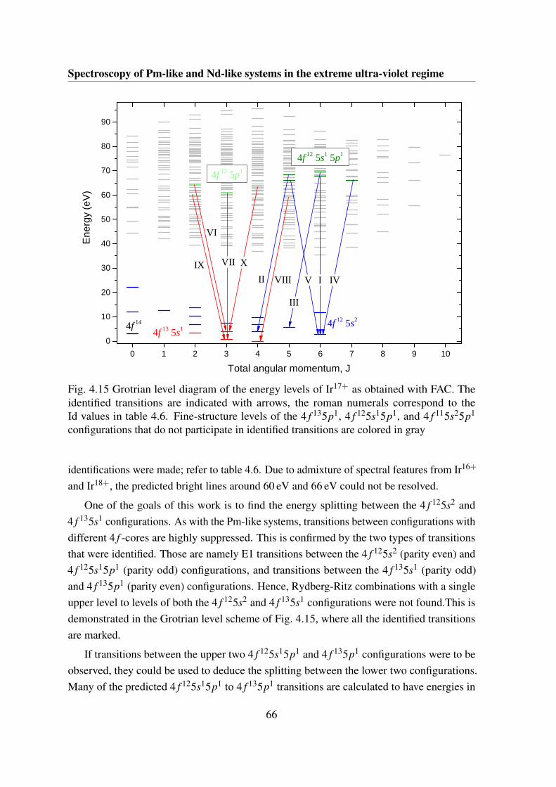
Spectroscopy of Pm-like and Nd-like systems in the extreme ultra-violet regime
0 1 2 3 4 5 6 7 8 9 1 00
1 0
2 0
3 0
4 0
5 0
6 0
7 0
8 0
9 0
I XV I I I
V I
I I
4 f 1 3 5 p 1
4 f 1 2 5 s 1 5 p 1
4 f 1 3 5 s 14 f 1 4
Ene
rgy
(eV
)
T o t a l a n g u l a r m o m e n t u m , J
4 f 1 2 5 s 2
I I I
I VIV
XV I I
Fig. 4.15 Grotrian level diagram of the energy levels of Ir17+ as obtained with FAC. Theidentified transitions are indicated with arrows, the roman numerals correspond to theId values in table 4.6. Fine-structure levels of the 4 f 135p1, 4 f 125s15p1, and 4 f 115s25p1
configurations that do not participate in identified transitions are colored in gray
identifications were made; refer to table 4.6. Due to admixture of spectral features from Ir16+
and Ir18+, the predicted bright lines around 60 eV and 66 eV could not be resolved.
One of the goals of this work is to find the energy splitting between the 4 f 125s2 and4 f 135s1 configurations. As with the Pm-like systems, transitions between configurations withdifferent 4 f -cores are highly suppressed. This is confirmed by the two types of transitionsthat were identified. Those are namely E1 transitions between the 4 f 125s2 (parity even) and4 f 125s15p1 (parity odd) configurations, and transitions between the 4 f 135s1 (parity odd)and 4 f 135p1 (parity even) configurations. Hence, Rydberg-Ritz combinations with a singleupper level to levels of both the 4 f 125s2 and 4 f 135s1 configurations were not found.This isdemonstrated in the Grotrian level scheme of Fig. 4.15, where all the identified transitionsare marked.
If transitions between the upper two 4 f 125s15p1 and 4 f 135p1 configurations were to beobserved, they could be used to deduce the splitting between the lower two configurations.Many of the predicted 4 f 125s15p1 to 4 f 135p1 transitions are calculated to have energies in
66
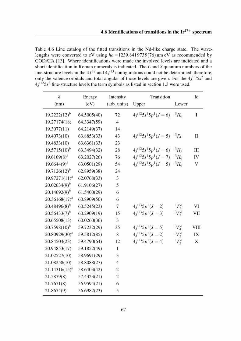
4.6 Identifications of transitions in the Ir17+ spectrum
Table 4.6 Line catalog of the fitted transitions in the Nd-like charge state. The wave-lengths were converted to eV using hc =1239.8419739(76) nm eV as recommended byCODATA [13]. Where identifications were made the involved levels are indicated and ashort identification in Roman numerals is indicated. The L and S quantum numbers of thefine-structure levels in the 4 f 12 and 4 f 13 configurations could not be determined, therefore,only the valence orbitals and total angular of those levels are given. For the 4 f 135s2 and4 f 125s2 fine-structure levels the term symbols as listed in section 1.3 were used.
λ Energy Intensity Transition Id(nm) (eV) (arb. units) Upper Lower
19.2222(12)b 64.5005(40) 72 4 f 125s15p1(J = 6) 3H6 I19.27174(18) 64.3347(59) 419.3077(11) 64.2149(37) 1419.4073(10) 63.8853(33) 43 4 f 125s15p1(J = 5) 3F4 II19.4833(10) 63.6361(33) 2319.5715(10)b 63.3494(32) 28 4 f 125s15p1(J = 6) 3H5 III19.6169(8)b 63.2027(26) 76 4 f 125s15p1(J = 7) 3H6 IV19.6644(9)b 63.0501(29) 54 4 f 125s15p1(J = 5) 3H6 V19.7126(12)b 62.8959(38) 2419.97271(11)b 62.0768(33) 320.02634(9)b 61.9106(27) 520.14692(9)b 61.5400(29) 620.36168(17)b 60.8909(50) 620.48496(8)b 60.5245(23) 7 4 f 135p1(J = 2) 1Fo
3 VI20.56433(7)b 60.2909(19) 15 4 f 135p1(J = 3) 3Fo
3 VII20.65508(13) 60.0260(36) 320.7598(10)b 59.7232(29) 35 4 f 135p1(J = 5) 3Fo
4 VIII20.80929(30)b 59.5812(85) 8 4 f 135p1(J = 2) 3Fo
3 IX20.84504(23) 59.4790(64) 12 4 f 135p1(J = 4) 1Fo
3 X20.94853(17) 59.1852(49) 121.02527(10) 58.9691(29) 321.08258(10) 58.8088(27) 421.14316(15)b 58.6403(42) 221.5879(8) 57.4323(21) 221.7671(8) 56.9594(21) 621.8674(9) 56.6982(23) 5
67
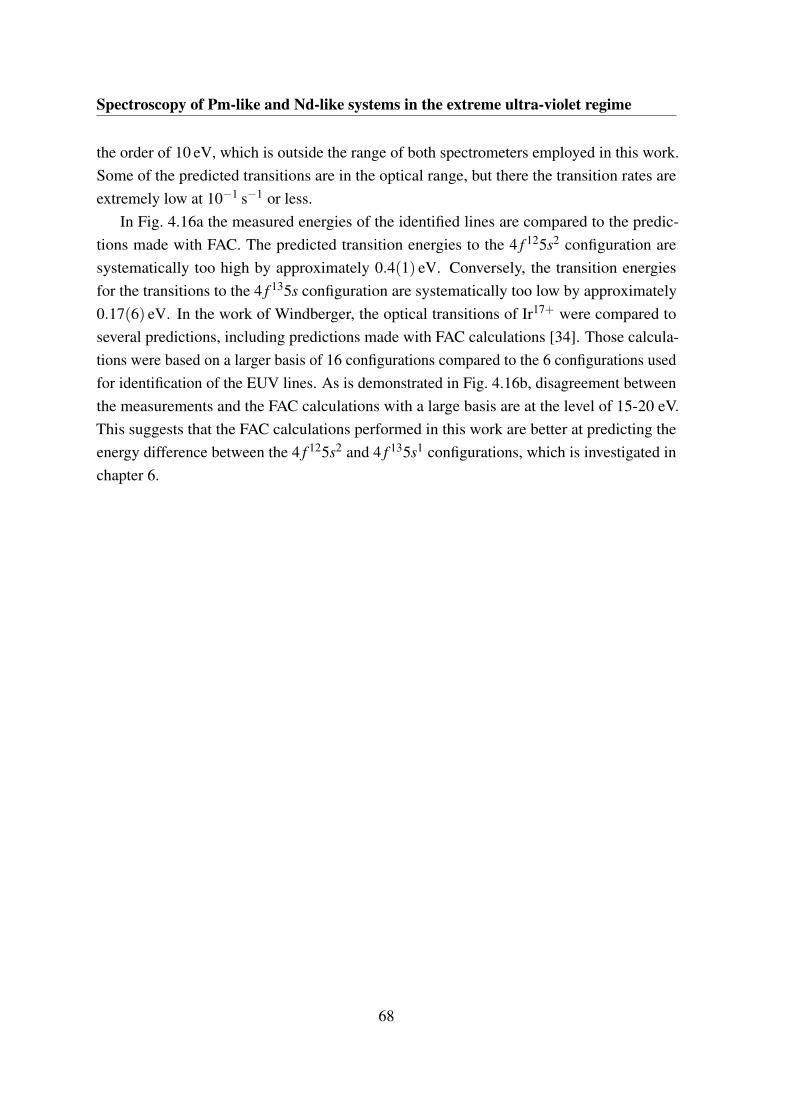
Spectroscopy of Pm-like and Nd-like systems in the extreme ultra-violet regime
the order of 10 eV, which is outside the range of both spectrometers employed in this work.Some of the predicted transitions are in the optical range, but there the transition rates areextremely low at 10−1 s−1 or less.
In Fig. 4.16a the measured energies of the identified lines are compared to the predic-tions made with FAC. The predicted transition energies to the 4 f 125s2 configuration aresystematically too high by approximately 0.4(1) eV. Conversely, the transition energiesfor the transitions to the 4 f 135s configuration are systematically too low by approximately0.17(6) eV. In the work of Windberger, the optical transitions of Ir17+ were compared toseveral predictions, including predictions made with FAC calculations [34]. Those calcula-tions were based on a larger basis of 16 configurations compared to the 6 configurations usedfor identification of the EUV lines. As is demonstrated in Fig. 4.16b, disagreement betweenthe measurements and the FAC calculations with a large basis are at the level of 15-20 eV.This suggests that the FAC calculations performed in this work are better at predicting theenergy difference between the 4 f 125s2 and 4 f 135s1 configurations, which is investigated inchapter 6.
68
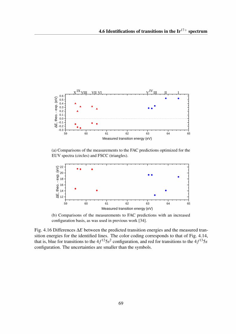
4.6 Identifications of transitions in the Ir17+ spectrum
5 9 6 0 6 1 6 2 6 3 6 4 6 5- 0 . 3- 0 . 2- 0 . 10 . 00 . 10 . 20 . 30 . 40 . 50 . 6
X I X V I I I V I I V I V I V I I I I I
∆E, t
heo.
- ex
p. (e
V)
M e a s u r e d t r a n s i t i o n e n e r g y ( e V )
I
(a) Comparisons of the measurements to the FAC predictions optimized for theEUV spectra (circles) and FSCC (triangles).
5 9 6 0 6 1 6 2 6 3 6 4 6 5
1 2
1 4
1 6
1 8
2 0
2 2
∆E, t
heo.
- ex
p. (e
V)
M e a s u r e d t r a n s i t i o n e n e r g y ( e V )
(b) Comparisons of the measurements to FAC predictions with an increasedconfiguration basis, as was used in previous work [34].
Fig. 4.16 Differences ∆E between the predicted transition energies and the measured tran-sition energies for the identified lines. The color coding corresponds to that of Fig. 4.14,that is, blue for transitions to the 4 f 125s2 configuration, and red for transitions to the 4 f 135sconfiguration. The uncertainties are smaller than the symbols.
69

Chapter 5
Spectroscopy in the optical regime
Non; mais Dieu a donné à l’homme l’intelligence pour venir en aide à la pauvretéde ses sens: je me suis procuré de la lumière.
Le Compte de Monte-Cristo, Alexandre Dumas
When asked how he could read and write in the darkness of his dungeon, Abbé Faria gavethe answer cited above. The statement more or less translates to ’Man has the intelligence toaid his mediocre senses, therefore, I made a light source.’. This can be applied to much of thework of experimental physicists. Examples include the improvements made to telescopes byGalileo Galilei, to more recent high-tech advances such as optical frequency combs and theLIGO interferometers [33, 135]. Physicists have always relied on ingenuity to improve theirobservational capabilities. In this chapter the setup and data analysis methods, which wereemployed to investigate extremely weak optical transitions of ions in an EBIT, are described.
5.1 The optical spectrometer setup
To measure the wavelengths of the fluorescence light emitted from the ion cloud in theEBIT, a grating spectrometer was employed. A telescope system and the so-called periscopebox were used to focus the image of the ion cloud on the entrance slit of the spectrometer.Light from a hallow cathode lamp could be imaged on the entrance slit of the spectrometerfor calibration purposes. The setup had previously been employed to investigate opticaltransitions in several other highly charged ions (HCI) [136, 137, 130, 138]). Next follows adescription of the individual components of the setup. An overview of the full setup, fromlight source to camera for recording of the spectra, is shown in Fig. 5.1. Since the camerahad recently been replaced with a newer model, details concerning the performance of the
71
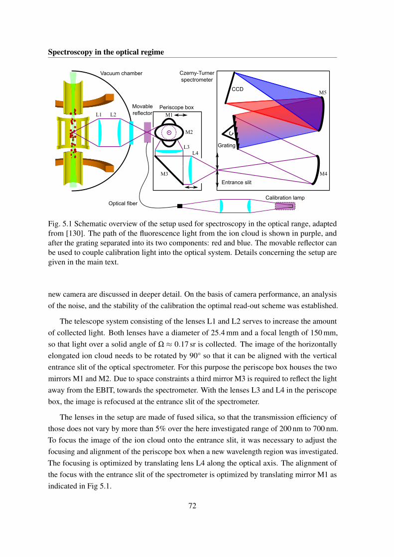
Spectroscopy in the optical regime
L1 L2
Vacuum chamber
Periscope box
Czerny-Turnerspectrometer
M1
M2
L3
M3
Entrance slit
M4
L4
M5CCD
Grating
Calibration lamp
Movablereflector
Optical fiber
Fig. 5.1 Schematic overview of the setup used for spectroscopy in the optical range, adaptedfrom [130]. The path of the fluorescence light from the ion cloud is shown in purple, andafter the grating separated into its two components: red and blue. The movable reflector canbe used to couple calibration light into the optical system. Details concerning the setup aregiven in the main text.
new camera are discussed in deeper detail. On the basis of camera performance, an analysisof the noise, and the stability of the calibration the optimal read-out scheme was established.
The telescope system consisting of the lenses L1 and L2 serves to increase the amountof collected light. Both lenses have a diameter of 25.4 mm and a focal length of 150 mm,so that light over a solid angle of Ω ≈ 0.17 sr is collected. The image of the horizontallyelongated ion cloud needs to be rotated by 90° so that it can be aligned with the verticalentrance slit of the optical spectrometer. For this purpose the periscope box houses the twomirrors M1 and M2. Due to space constraints a third mirror M3 is required to reflect the lightaway from the EBIT, towards the spectrometer. With the lenses L3 and L4 in the periscopebox, the image is refocused at the entrance slit of the spectrometer.
The lenses in the setup are made of fused silica, so that the transmission efficiency ofthose does not vary by more than 5% over the here investigated range of 200 nm to 700 nm.To focus the image of the ion cloud onto the entrance slit, it was necessary to adjust thefocusing and alignment of the periscope box when a new wavelength region was investigated.The focusing is optimized by translating lens L4 along the optical axis. The alignment ofthe focus with the entrance slit of the spectrometer is optimized by translating mirror M1 asindicated in Fig 5.1.
72
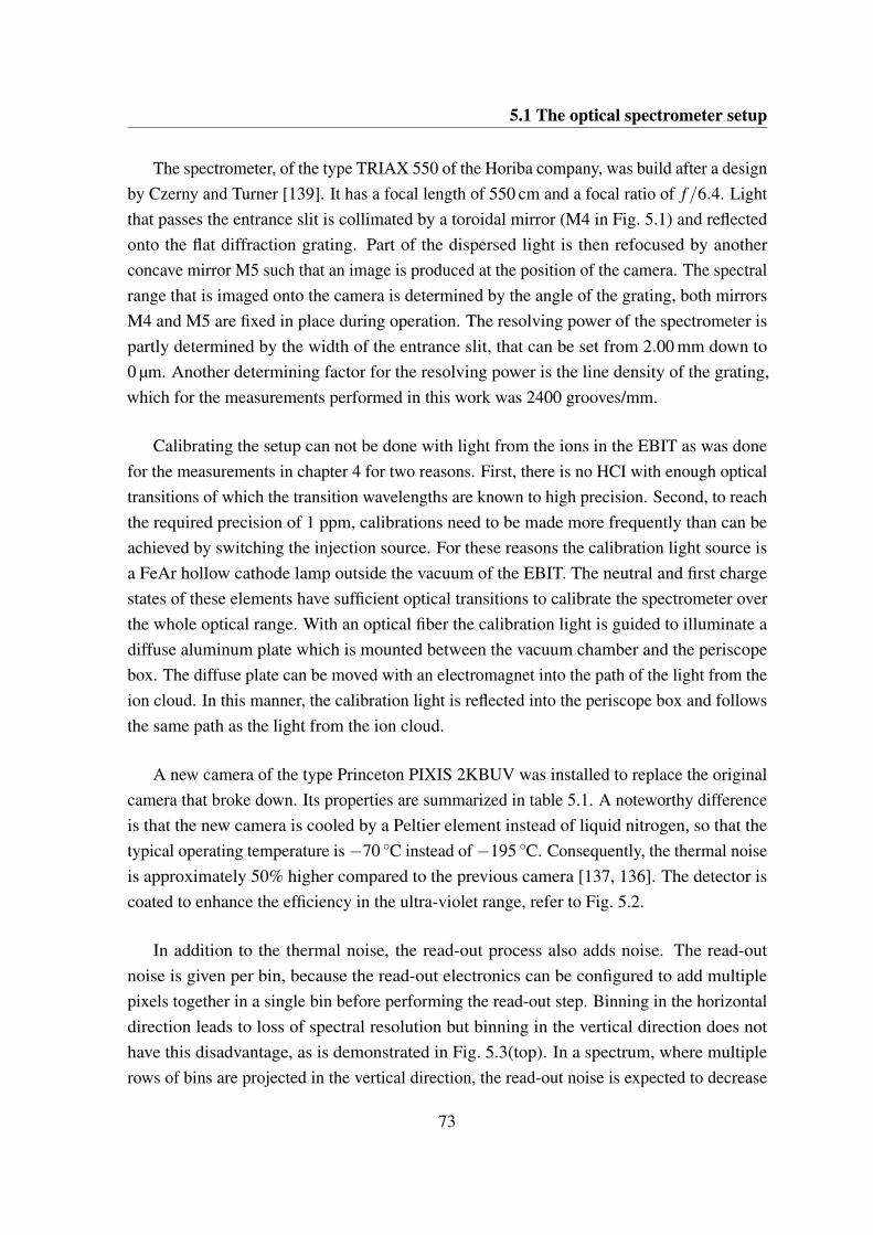
5.1 The optical spectrometer setup
The spectrometer, of the type TRIAX 550 of the Horiba company, was build after a designby Czerny and Turner [139]. It has a focal length of 550 cm and a focal ratio of f/6.4. Lightthat passes the entrance slit is collimated by a toroidal mirror (M4 in Fig. 5.1) and reflectedonto the flat diffraction grating. Part of the dispersed light is then refocused by anotherconcave mirror M5 such that an image is produced at the position of the camera. The spectralrange that is imaged onto the camera is determined by the angle of the grating, both mirrorsM4 and M5 are fixed in place during operation. The resolving power of the spectrometer ispartly determined by the width of the entrance slit, that can be set from 2.00 mm down to0 µm. Another determining factor for the resolving power is the line density of the grating,which for the measurements performed in this work was 2400 grooves/mm.
Calibrating the setup can not be done with light from the ions in the EBIT as was donefor the measurements in chapter 4 for two reasons. First, there is no HCI with enough opticaltransitions of which the transition wavelengths are known to high precision. Second, to reachthe required precision of 1 ppm, calibrations need to be made more frequently than can beachieved by switching the injection source. For these reasons the calibration light source isa FeAr hollow cathode lamp outside the vacuum of the EBIT. The neutral and first chargestates of these elements have sufficient optical transitions to calibrate the spectrometer overthe whole optical range. With an optical fiber the calibration light is guided to illuminate adiffuse aluminum plate which is mounted between the vacuum chamber and the periscopebox. The diffuse plate can be moved with an electromagnet into the path of the light from theion cloud. In this manner, the calibration light is reflected into the periscope box and followsthe same path as the light from the ion cloud.
A new camera of the type Princeton PIXIS 2KBUV was installed to replace the originalcamera that broke down. Its properties are summarized in table 5.1. A noteworthy differenceis that the new camera is cooled by a Peltier element instead of liquid nitrogen, so that thetypical operating temperature is −70 C instead of −195 C. Consequently, the thermal noiseis approximately 50% higher compared to the previous camera [137, 136]. The detector iscoated to enhance the efficiency in the ultra-violet range, refer to Fig. 5.2.
In addition to the thermal noise, the read-out process also adds noise. The read-outnoise is given per bin, because the read-out electronics can be configured to add multiplepixels together in a single bin before performing the read-out step. Binning in the horizontaldirection leads to loss of spectral resolution but binning in the vertical direction does nothave this disadvantage, as is demonstrated in Fig. 5.3(top). In a spectrum, where multiplerows of bins are projected in the vertical direction, the read-out noise is expected to decrease
73

Spectroscopy in the optical regime
Table 5.1 Properties and settings of the PIXIS 2KBUV camera [140].
Property Value
Dimensions 2048 × 512 pixelsPixel size 13.5 × 13.5 µm2
Operating temperature −70 CRead-out noise, Nbin
RO 3.74 e− / binThermal noise 1.59 e− / pixel hourRead-out frequency 100 kHzPre-amplifier setting Low-noise outputConversion gain 1.01 e− / count
as
NRO = NbinRO
√512
n, (5.1)
where n is the number of pixels that are added in one bin. The predicted behavior can beobserved in Fig. 5.3(bottom). Clearly increased binning reduces the read-out noise in thespectrum, but some of the vertical information is needed for the removal of cosmics and forthe correction of optical aberrations. Experience shows that a binning of 64 pixels per bin,i.e. dividing the CCD into 8 rows, gives sufficient vertical information to remove the cosmicsthat accumulate over half an hour with high fidelity.
5.2 Measurement procedure
Several hours, or even days, of integration time were required to achieve a good enoughsignal to noise ratio for the investigated lines. This is because the transitions rates of theinvestigated lines are in the range of only 1−100 s−1. To ensure a high quality of the data,a procedure was developed which prevents some of the pitfalls that would otherwise occur.The details and reasoning behind the procedure will be described next, but first the steps aresummarized as:
1. Optimize spectrometer for the wavelength of interest
2. Acquire background spectrum
3. Acquire calibration spectrum
74
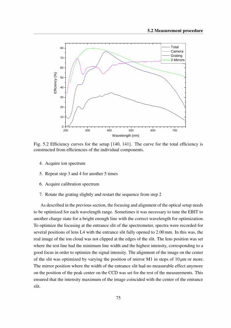
5.2 Measurement procedure
2 0 0 3 0 0 4 0 0 5 0 0 6 0 0 7 0 00
1 0
2 0
3 0
4 0
5 0
6 0
7 0
8 0 T o t a l C a m e r a G r a t i n g 3 M i r r o r s
Effi
cien
cy (%
)
W a v e l e n g t h ( n m )
Fig. 5.2 Efficiency curves for the setup [140, 141]. The curve for the total efficiency isconstructed from efficiencies of the individual components.
4. Acquire ion spectrum
5. Repeat step 3 and 4 for another 5 times
6. Acquire calibration spectrum
7. Rotate the grating slightly and restart the sequence from step 2
As described in the previous section, the focusing and alignment of the optical setup needsto be optimized for each wavelength range. Sometimes it was necessary to tune the EBIT toanother charge state for a bright enough line with the correct wavelength for optimization.To optimize the focusing at the entrance slit of the spectrometer, spectra were recorded forseveral positions of lens L4 with the entrance slit fully opened to 2.00 mm. In this was, thereal image of the ion cloud was not clipped at the edges of the slit. The lens position was setwhere the test line had the minimum line width and the highest intensity, corresponding to agood focus in order to optimize the signal intensity. The alignment of the image on the centerof the slit was optimized by varying the position of mirror M1 in steps of 10 µm or more.The mirror position where the width of the entrance slit had no measurable effect anymoreon the position of the peak center on the CCD was set for the rest of the measurements. Thisensured that the intensity maximum of the image coincided with the center of the entranceslit.
75
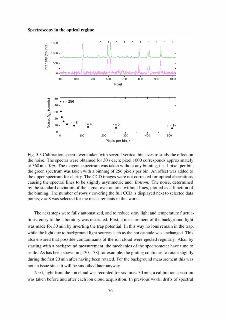
Spectroscopy in the optical regime
3 0 0 4 0 0 5 0 0 6 0 0 7 0 0 8 0 0 9 0 0 1 0 0 0
0
5 0 0
1 0 0 0
1 5 0 0In
tens
ity (c
ount
s)
P i x e l
0 1 0 0 2 0 0 3 0 0 4 0 0 5 0 00
1 0
2 0
3 0
4 0
5 0r = 2 5 6
r = 8 r = 4 r = 2
B
Noi
se, N
RO (c
ount
s)
P i x e l s p e r b i n , n
r = 1
Fig. 5.3 Calibration spectra were taken with several vertical bin sizes to study the effect onthe noise. The spectra were obtained for 30 s each; pixel 1000 corresponds approximatelyto 360 nm. Top: The magenta spectrum was taken without any binning, i.e. 1 pixel per bin,the green spectrum was taken with a binning of 256 pixels per bin. An offset was added tothe upper spectrum for clarity. The CCD images were not corrected for optical aberrations,causing the spectral lines to be slightly asymmetric and. Bottom: The noise, determinedby the standard deviation of the signal over an area without lines, plotted as a function ofthe binning. The number of rows r covering the full CCD is displayed next to selected datapoints; r = 8 was selected for the measurements in this work.
The next steps were fully automatized, and to reduce stray light and temperature fluctua-tions, entry to the laboratory was restricted. First, a measurement of the background lightwas made for 30 min by inverting the trap potential. In this way no ions remain in the trap,while the light due to background light sources such as the hot cathode was unchanged. Thisalso ensured that possible contaminants of the ion cloud were ejected regularly. Also, bystarting with a background measurement, the mechanics of the spectrometer have time tosettle. As has been shown in [130, 138] for example, the grating continues to rotate slightlyduring the first 20 min after having been rotated. For the background measurement this wasnot an issue since it will be smoothed later anyway.
Next, light from the ion cloud was recorded for six times 30 min, a calibration spectrumwas taken before and after each ion cloud acquisition. In previous work, drifts of spectral
76
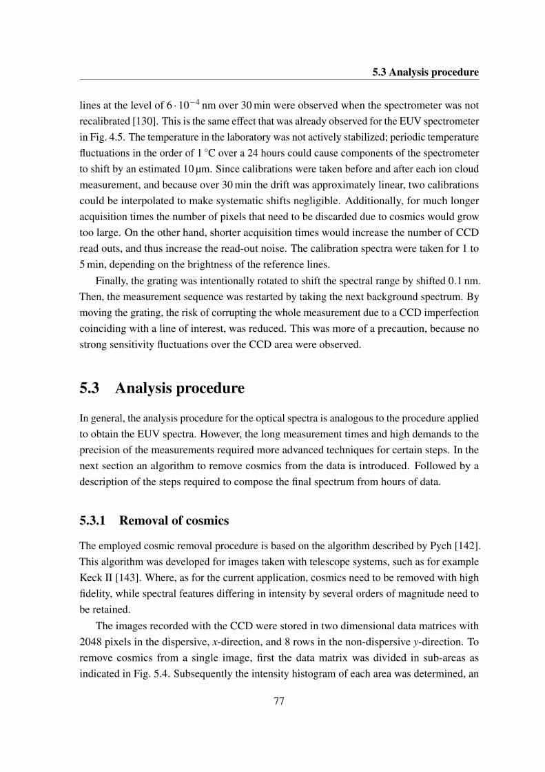
5.3 Analysis procedure
lines at the level of 6 ·10−4 nm over 30 min were observed when the spectrometer was notrecalibrated [130]. This is the same effect that was already observed for the EUV spectrometerin Fig. 4.5. The temperature in the laboratory was not actively stabilized; periodic temperaturefluctuations in the order of 1 C over a 24 hours could cause components of the spectrometerto shift by an estimated 10 µm. Since calibrations were taken before and after each ion cloudmeasurement, and because over 30 min the drift was approximately linear, two calibrationscould be interpolated to make systematic shifts negligible. Additionally, for much longeracquisition times the number of pixels that need to be discarded due to cosmics would growtoo large. On the other hand, shorter acquisition times would increase the number of CCDread outs, and thus increase the read-out noise. The calibration spectra were taken for 1 to5 min, depending on the brightness of the reference lines.
Finally, the grating was intentionally rotated to shift the spectral range by shifted 0.1 nm.Then, the measurement sequence was restarted by taking the next background spectrum. Bymoving the grating, the risk of corrupting the whole measurement due to a CCD imperfectioncoinciding with a line of interest, was reduced. This was more of a precaution, because nostrong sensitivity fluctuations over the CCD area were observed.
5.3 Analysis procedure
In general, the analysis procedure for the optical spectra is analogous to the procedure appliedto obtain the EUV spectra. However, the long measurement times and high demands to theprecision of the measurements required more advanced techniques for certain steps. In thenext section an algorithm to remove cosmics from the data is introduced. Followed by adescription of the steps required to compose the final spectrum from hours of data.
5.3.1 Removal of cosmics
The employed cosmic removal procedure is based on the algorithm described by Pych [142].This algorithm was developed for images taken with telescope systems, such as for exampleKeck II [143]. Where, as for the current application, cosmics need to be removed with highfidelity, while spectral features differing in intensity by several orders of magnitude need tobe retained.
The images recorded with the CCD were stored in two dimensional data matrices with2048 pixels in the dispersive, x-direction, and 8 rows in the non-dispersive y-direction. Toremove cosmics from a single image, first the data matrix was divided in sub-areas asindicated in Fig. 5.4. Subsequently the intensity histogram of each area was determined, an
77
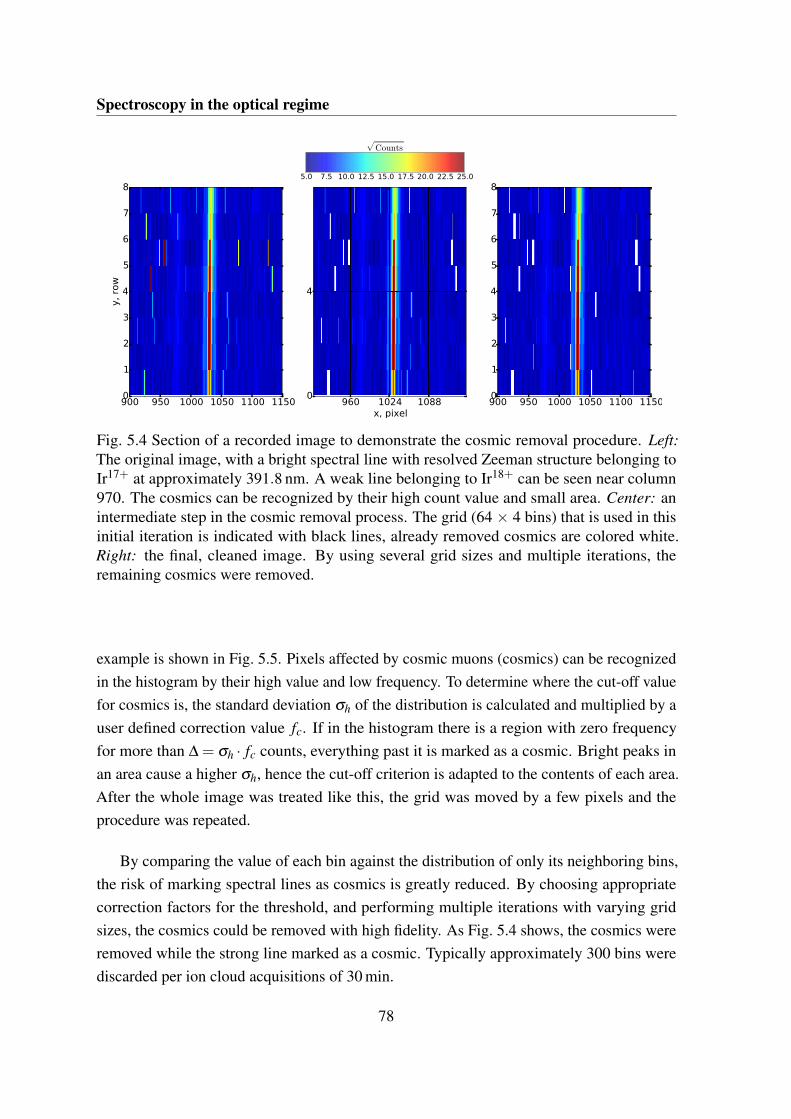
Spectroscopy in the optical regime
5.0 7.5 10.0 12.5 15.0 17.5 20.0 22.5 25.0
√Counts
900 950 1000 1050 1100 11500
1
2
3
4
5
6
7
8
y,
row
960 1024 1088x, pixel
0
4
900 950 1000 1050 1100 11500
1
2
3
4
5
6
7
8
Fig. 5.4 Section of a recorded image to demonstrate the cosmic removal procedure. Left:The original image, with a bright spectral line with resolved Zeeman structure belonging toIr17+ at approximately 391.8 nm. A weak line belonging to Ir18+ can be seen near column970. The cosmics can be recognized by their high count value and small area. Center: anintermediate step in the cosmic removal process. The grid (64 × 4 bins) that is used in thisinitial iteration is indicated with black lines, already removed cosmics are colored white.Right: the final, cleaned image. By using several grid sizes and multiple iterations, theremaining cosmics were removed.
example is shown in Fig. 5.5. Pixels affected by cosmic muons (cosmics) can be recognizedin the histogram by their high value and low frequency. To determine where the cut-off valuefor cosmics is, the standard deviation σh of the distribution is calculated and multiplied by auser defined correction value fc. If in the histogram there is a region with zero frequencyfor more than ∆ = σh · fc counts, everything past it is marked as a cosmic. Bright peaks inan area cause a higher σh, hence the cut-off criterion is adapted to the contents of each area.After the whole image was treated like this, the grid was moved by a few pixels and theprocedure was repeated.
By comparing the value of each bin against the distribution of only its neighboring bins,the risk of marking spectral lines as cosmics is greatly reduced. By choosing appropriatecorrection factors for the threshold, and performing multiple iterations with varying gridsizes, the cosmics could be removed with high fidelity. As Fig. 5.4 shows, the cosmics wereremoved while the strong line marked as a cosmic. Typically approximately 300 bins werediscarded per ion cloud acquisitions of 30 min.
78
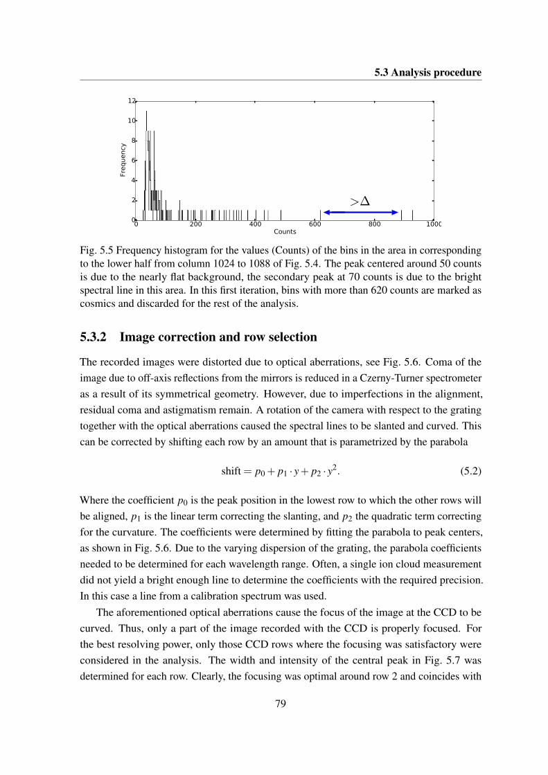
5.3 Analysis procedure
0 200 400 600 800 1000Counts
0
2
4
6
8
10
12
Frequency
>∆
Fig. 5.5 Frequency histogram for the values (Counts) of the bins in the area in correspondingto the lower half from column 1024 to 1088 of Fig. 5.4. The peak centered around 50 countsis due to the nearly flat background, the secondary peak at 70 counts is due to the brightspectral line in this area. In this first iteration, bins with more than 620 counts are marked ascosmics and discarded for the rest of the analysis.
5.3.2 Image correction and row selection
The recorded images were distorted due to optical aberrations, see Fig. 5.6. Coma of theimage due to off-axis reflections from the mirrors is reduced in a Czerny-Turner spectrometeras a result of its symmetrical geometry. However, due to imperfections in the alignment,residual coma and astigmatism remain. A rotation of the camera with respect to the gratingtogether with the optical aberrations caused the spectral lines to be slanted and curved. Thiscan be corrected by shifting each row by an amount that is parametrized by the parabola
shift = p0 + p1 · y+ p2 · y2. (5.2)
Where the coefficient p0 is the peak position in the lowest row to which the other rows willbe aligned, p1 is the linear term correcting the slanting, and p2 the quadratic term correctingfor the curvature. The coefficients were determined by fitting the parabola to peak centers,as shown in Fig. 5.6. Due to the varying dispersion of the grating, the parabola coefficientsneeded to be determined for each wavelength range. Often, a single ion cloud measurementdid not yield a bright enough line to determine the coefficients with the required precision.In this case a line from a calibration spectrum was used.
The aforementioned optical aberrations cause the focus of the image at the CCD to becurved. Thus, only a part of the image recorded with the CCD is properly focused. Forthe best resolving power, only those CCD rows where the focusing was satisfactory wereconsidered in the analysis. The width and intensity of the central peak in Fig. 5.7 wasdetermined for each row. Clearly, the focusing was optimal around row 2 and coincides with
79
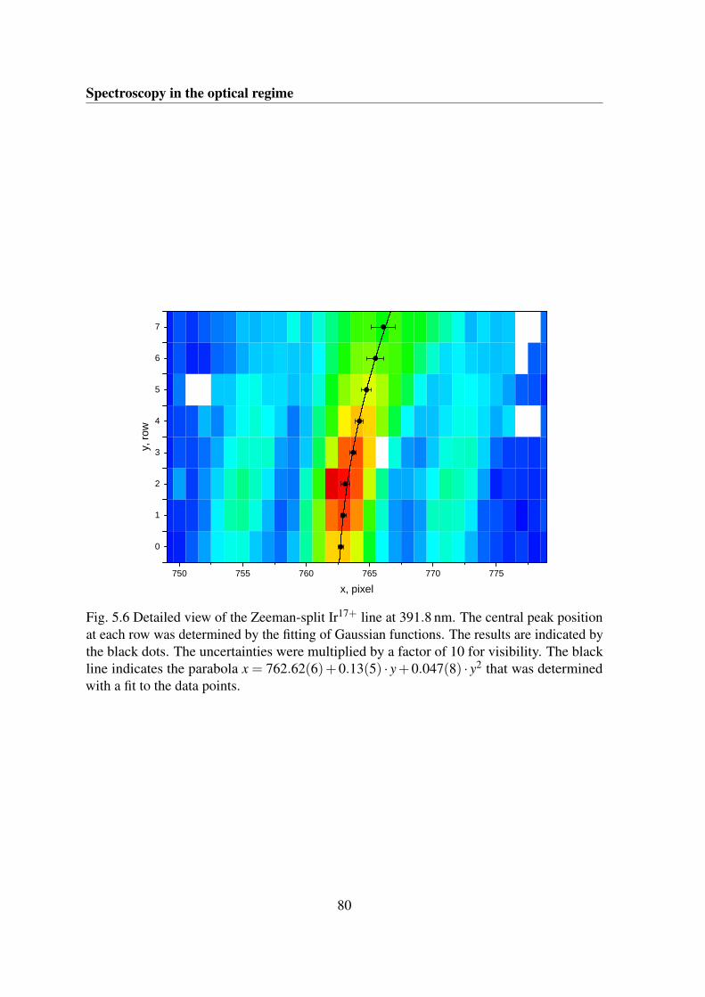
Spectroscopy in the optical regime
7 5 0 7 5 5 7 6 0 7 6 5 7 7 0 7 7 5
0
1
2
3
4
5
6
7
8
x , p i x e l
y, ro
w
Fig. 5.6 Detailed view of the Zeeman-split Ir17+ line at 391.8 nm. The central peak positionat each row was determined by the fitting of Gaussian functions. The results are indicated bythe black dots. The uncertainties were multiplied by a factor of 10 for visibility. The blackline indicates the parabola x = 762.62(6)+0.13(5) · y+0.047(8) · y2 that was determinedwith a fit to the data points.
80
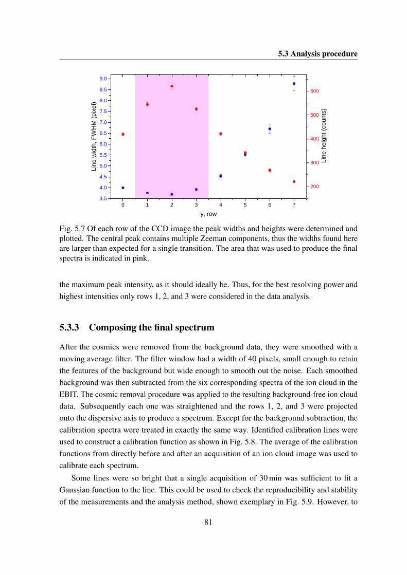
5.3 Analysis procedure
0 1 2 3 4 5 6 73 . 5
4 . 0
4 . 5
5 . 0
5 . 5
6 . 0
6 . 5
7 . 0
7 . 5
8 . 0
8 . 5
9 . 0
y , r o w
Line
wid
th, F
WH
M (p
ixel
)
2 0 0
3 0 0
4 0 0
5 0 0
6 0 0
Lin
e he
ight
(cou
nts)
Fig. 5.7 Of each row of the CCD image the peak widths and heights were determined andplotted. The central peak contains multiple Zeeman components, thus the widths found hereare larger than expected for a single transition. The area that was used to produce the finalspectra is indicated in pink.
the maximum peak intensity, as it should ideally be. Thus, for the best resolving power andhighest intensities only rows 1, 2, and 3 were considered in the data analysis.
5.3.3 Composing the final spectrum
After the cosmics were removed from the background data, they were smoothed with amoving average filter. The filter window had a width of 40 pixels, small enough to retainthe features of the background but wide enough to smooth out the noise. Each smoothedbackground was then subtracted from the six corresponding spectra of the ion cloud in theEBIT. The cosmic removal procedure was applied to the resulting background-free ion clouddata. Subsequently each one was straightened and the rows 1, 2, and 3 were projectedonto the dispersive axis to produce a spectrum. Except for the background subtraction, thecalibration spectra were treated in exactly the same way. Identified calibration lines wereused to construct a calibration function as shown in Fig. 5.8. The average of the calibrationfunctions from directly before and after an acquisition of an ion cloud image was used tocalibrate each spectrum.
Some lines were so bright that a single acquisition of 30 min was sufficient to fit aGaussian function to the line. This could be used to check the reproducibility and stabilityof the measurements and the analysis method, shown exemplary in Fig. 5.9. However, to
81
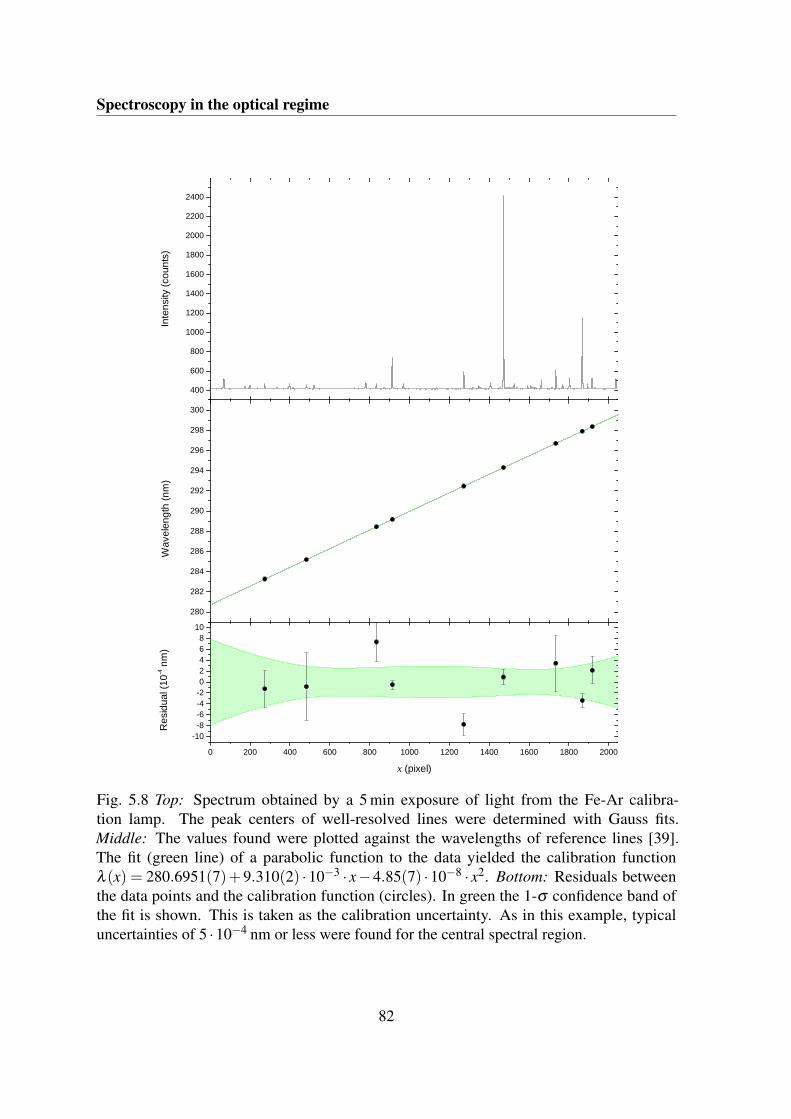
Spectroscopy in the optical regime
4 0 0
6 0 0
8 0 0
1 0 0 0
1 2 0 0
1 4 0 0
1 6 0 0
1 8 0 0
2 0 0 0
2 2 0 0
2 4 0 0
2 8 0
2 8 2
2 8 4
2 8 6
2 8 8
2 9 0
2 9 2
2 9 4
2 9 6
2 9 8
3 0 0
0 2 0 0 4 0 0 6 0 0 8 0 0 1 0 0 0 1 2 0 0 1 4 0 0 1 6 0 0 1 8 0 0 2 0 0 0
- 1 0- 8- 6- 4- 202468
1 0
Inte
nsity
(cou
nts)
Wav
elen
gth
(nm
)R
esid
ual (
10-4 n
m)
x ( p i x e l )
Fig. 5.8 Top: Spectrum obtained by a 5 min exposure of light from the Fe-Ar calibra-tion lamp. The peak centers of well-resolved lines were determined with Gauss fits.Middle: The values found were plotted against the wavelengths of reference lines [39].The fit (green line) of a parabolic function to the data yielded the calibration functionλ (x) = 280.6951(7)+9.310(2) ·10−3 · x−4.85(7) ·10−8 · x2. Bottom: Residuals betweenthe data points and the calibration function (circles). In green the 1-σ confidence band ofthe fit is shown. This is taken as the calibration uncertainty. As in this example, typicaluncertainties of 5 ·10−4 nm or less were found for the central spectral region.
82
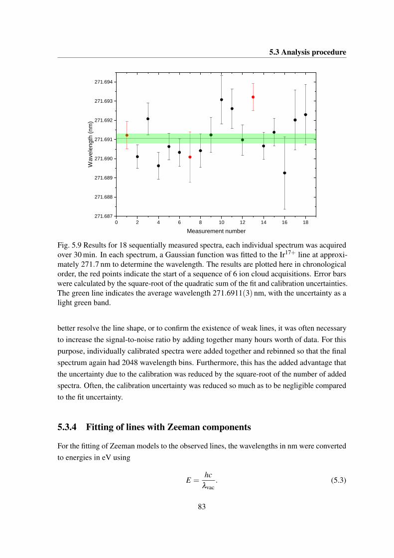
5.3 Analysis procedure
0 2 4 6 8 1 0 1 2 1 4 1 6 1 82 7 1 . 6 8 7
2 7 1 . 6 8 8
2 7 1 . 6 8 9
2 7 1 . 6 9 0
2 7 1 . 6 9 1
2 7 1 . 6 9 2
2 7 1 . 6 9 3
2 7 1 . 6 9 4W
avel
engt
h (n
m)
M e a s u r e m e n t n u m b e r
Fig. 5.9 Results for 18 sequentially measured spectra, each individual spectrum was acquiredover 30 min. In each spectrum, a Gaussian function was fitted to the Ir17+ line at approxi-mately 271.7 nm to determine the wavelength. The results are plotted here in chronologicalorder, the red points indicate the start of a sequence of 6 ion cloud acquisitions. Error barswere calculated by the square-root of the quadratic sum of the fit and calibration uncertainties.The green line indicates the average wavelength 271.6911(3) nm, with the uncertainty as alight green band.
better resolve the line shape, or to confirm the existence of weak lines, it was often necessaryto increase the signal-to-noise ratio by adding together many hours worth of data. For thispurpose, individually calibrated spectra were added together and rebinned so that the finalspectrum again had 2048 wavelength bins. Furthermore, this has the added advantage thatthe uncertainty due to the calibration was reduced by the square-root of the number of addedspectra. Often, the calibration uncertainty was reduced so much as to be negligible comparedto the fit uncertainty.
5.3.4 Fitting of lines with Zeeman components
For the fitting of Zeeman models to the observed lines, the wavelengths in nm were convertedto energies in eV using
E =hc
λvac. (5.3)
83
Spectroscopy in the optical regime
The recommended values for Planck’s constant h and the speed of light c were taken fromCODATA, hc=1239.8419739(76) nm eV [13]. The wavelength λvac used for the conversionis the wavelength in vacuum. Because the spectrometer was placed in air, the measuredwavelengths needed to be corrected for the refractive properties of air. The refractive indexof air nair depends on factors such as air pressure and humidity, which were not closelymonitored during the measurements. However, the reference lines used for the calibrationwere taken under well controlled conditions [144, 145]. So those wavelengths in air can beconverted to wavelengths in vacuum using [146, 147]
λvac = nairλvac (5.4)
nair = 1+10−8(
8342.13+2406030130−S2 +
1599738.9−S2
)(5.5)
with S =1000λair
. (5.6)
The model for the line shapes was based on the following assumptions which weremotivated in section 2.1.5. 1) Each spectral line has multiple Zeeman components with energydifferences ∆EZ(gi
j,gfj ) from the central transition energy E0. 2) The relative intensities
of the components within a ∆m group are determined by Clebsch-Gordan coefficients. 3)The efficiencies of the setup for the two orthogonal linear polarizations are parametrizedby A0 and A±1. 4) The Zeeman components are convolved with a Gaussian function with awidth wG. The fit function based on these assumptions is
f (E0,wG,A0,A±1,offset) = offset+∑A∆m⟨ j f (mi +∆m)1∆m| jimi⟩2
·Gaussian(E0 +∆EZ,wG). (5.7)
Here the sum is understood to be taken over all the transitions between the Zeeman levels.The g j-factors that are needed to determine the energy differences ∆EZ were calculatedemploying different techniques, see table 5.2. The two independently performed advancedcalculations (Oreshkina and Bergengut) give results that are consistent at the level of 1%,which suggests that the predictions are accurate at this level. For well-resolved lines, the g j-factors can be left as free fit parameters and thus extracted from the measurement. However,previous measurements found deviations between measurements and predictions at the10% level [130]. In these cases both the g j-factors of both upper and lower levels stronglydeviated from the predictions. This can be explained by the fact that the two g j-factors arecorrelated fit parameters. As shown in section 2.1.5, the difference between the g j-factorsdetermines the energy splitting within one ∆m group, while the value of the individual
84
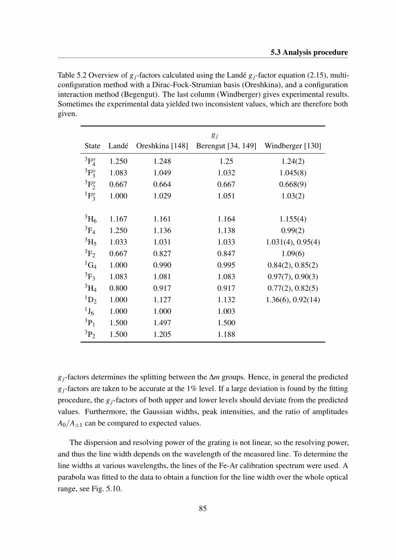
5.3 Analysis procedure
Table 5.2 Overview of g j-factors calculated using the Landé g j-factor equation (2.15), multi-configuration method with a Dirac-Fock-Strumian basis (Oreshkina), and a configurationinteraction method (Begengut). The last column (Windberger) gives experimental results.Sometimes the experimental data yielded two inconsistent values, which are therefore bothgiven.
g j
State Landé Oreshkina [148] Berengut [34, 149] Windberger [130]
3Fo4 1.250 1.248 1.25 1.24(2)
3Fo3 1.083 1.049 1.032 1.045(8)
3Fo2 0.667 0.664 0.667 0.668(9)
1Fo3 1.000 1.029 1.051 1.03(2)
3H6 1.167 1.161 1.164 1.155(4)3F4 1.250 1.136 1.138 0.99(2)3H5 1.033 1.031 1.033 1.031(4), 0.95(4)3F2 0.667 0.827 0.847 1.09(6)1G4 1.000 0.990 0.995 0.84(2), 0.85(2)3F3 1.083 1.081 1.083 0.97(7), 0.90(3)3H4 0.800 0.917 0.917 0.77(2), 0.82(5)1D2 1.000 1.127 1.132 1.36(6), 0.92(14)1J6 1.000 1.000 1.0033P1 1.500 1.497 1.5003P2 1.500 1.205 1.188
g j-factors determines the splitting between the ∆m groups. Hence, in general the predictedg j-factors are taken to be accurate at the 1% level. If a large deviation is found by the fittingprocedure, the g j-factors of both upper and lower levels should deviate from the predictedvalues. Furthermore, the Gaussian widths, peak intensities, and the ratio of amplitudesA0/A±1 can be compared to expected values.
The dispersion and resolving power of the grating is not linear, so the resolving power,and thus the line width depends on the wavelength of the measured line. To determine theline widths at various wavelengths, the lines of the Fe-Ar calibration spectrum were used. Aparabola was fitted to the data to obtain a function for the line width over the whole opticalrange, see Fig. 5.10.
85
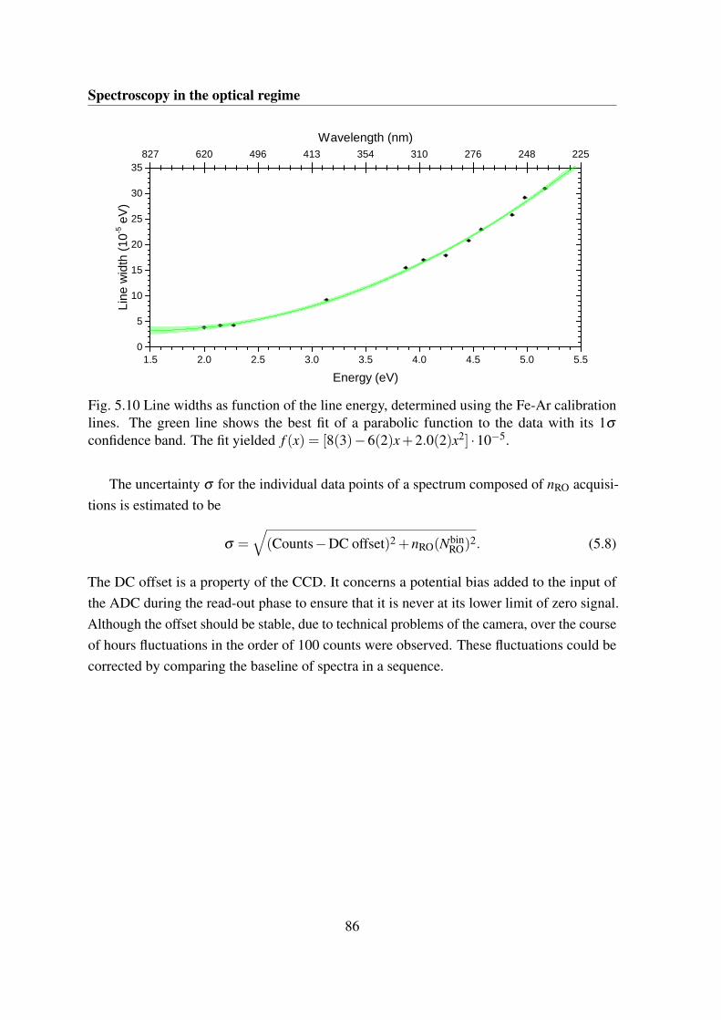
Spectroscopy in the optical regime
1 . 5 2 . 0 2 . 5 3 . 0 3 . 5 4 . 0 4 . 5 5 . 0 5 . 5
8 2 7 6 2 0 4 9 6 4 1 3 3 5 4 3 1 0 2 7 6 2 4 8 2 2 5
0
5
1 0
1 5
2 0
2 5
3 0
3 5
W a v e l e n g t h ( n m )Li
ne w
idth
(10-5
eV
)
E n e r g y ( e V )
Fig. 5.10 Line widths as function of the line energy, determined using the Fe-Ar calibrationlines. The green line shows the best fit of a parabolic function to the data with its 1σ
confidence band. The fit yielded f (x) = [8(3)−6(2)x+2.0(2)x2] ·10−5.
The uncertainty σ for the individual data points of a spectrum composed of nRO acquisi-tions is estimated to be
σ =√
(Counts−DC offset)2 +nRO(NbinRO)
2. (5.8)
The DC offset is a property of the CCD. It concerns a potential bias added to the input ofthe ADC during the read-out phase to ensure that it is never at its lower limit of zero signal.Although the offset should be stable, due to technical problems of the camera, over the courseof hours fluctuations in the order of 100 counts were observed. These fluctuations could becorrected by comparing the baseline of spectra in a sequence.
86
Chapter 6
Measurement and interpretation of theoptical spectra
In Ir17+ , the transitions with a high sensitivity to a variation of the fine-structure constant α
are those that take place between the 4 f 14, 4 f 135s1, and 4 f 125s2 configurations. As a resultof configuration mixing, there are E1 tranisitons taking place between them. However, due tothe small overlap between the wave functions of the configurations, their transition rates aretypically 10 s−1 or less. This low rate makes them suitable for precision laser spectroscopy.It also means that the transitions are difficult to observe. The optical transitions to the 4 f 14
configuration all require a change of total angular momentum ∆J ≥ 2, and are thereforethought to be too weak to be observed with the methods employed in this work. Severaloptical electric-dipole (E1) transitions between the 4 f 135s1, and 4 f 125s2 configurations areexpected to be strong enough to be observed, and are at the focus of this chapter. In earlierwork of our group, 11 magnetic dipole (M1) transitions taking place between fine-structurelevels of the same configuration were identified, see Fig. 6.1. Here, the remaining opticalM1 transitions were measured. These can be used in the search for so-called Rydberg-Ritzcombinations, where several measured transition energies can form a combination that addsup to zero; that is, they form a closed optical cycle. When a Rydberg-Ritz combination isfound that includes previously identified transitions, the assignment of the unidentified linescan often be inferred. This requires a high accuracy of the energy measurements in order toexclude fortuitous agreements. Here, the techniques described in chapter 5 are employed tosearch for and to measure several weak lines in the Ir17+ spectrum. Unidentified lines weretested for Rydberg-Ritz combinations that include interconfiguration transitions. SeveralE1 candidates were found, the line shapes were tested for their agreement with the Zeemanmodels.
87
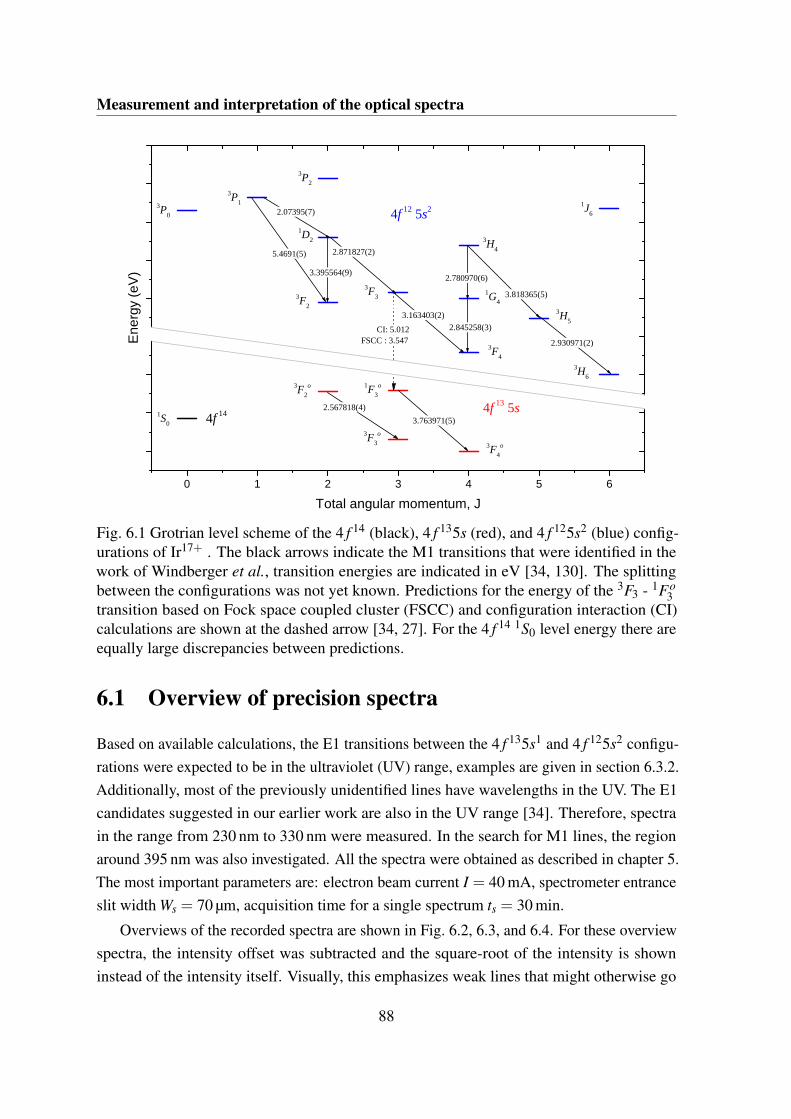
Measurement and interpretation of the optical spectra
0 1 2 3 4 5 6
4 f 1 2 5 s 2
4 f 1 3 5 s
Ene
rgy
(eV
)
T o t a l a n g u l a r m o m e n t u m , J
1 S 0
3 P 23 P 13 P 0
1 J 6
1 D 2 3 H 4
1 G 4
3 F 33 F 2
3 F 4
3 H 5
3 H 61 F 3
o3 F 2o
3 F 3o
3 F 4o
3 . 1 6 3 4 0 3 ( 2 )
3 . 3 9 5 5 6 4 ( 9 )
3 . 7 6 3 9 7 1 ( 5 )
2 . 0 7 3 9 5 ( 7 )
5 . 4 6 9 1 ( 5 ) 2 . 8 7 1 8 2 7 ( 2 )
2 . 7 8 0 9 7 0 ( 6 )
2 . 8 4 5 2 5 8 ( 3 )
3 . 8 1 8 3 6 5 ( 5 )
2 . 9 3 0 9 7 1 ( 2 )
2 . 5 6 7 8 1 8 ( 4 )4 f 1 4
C I : 5 . 0 1 2F S C C : 3 . 5 4 7
Fig. 6.1 Grotrian level scheme of the 4 f 14 (black), 4 f 135s (red), and 4 f 125s2 (blue) config-urations of Ir17+ . The black arrows indicate the M1 transitions that were identified in thework of Windberger et al., transition energies are indicated in eV [34, 130]. The splittingbetween the configurations was not yet known. Predictions for the energy of the 3F3 - 1Fo
3transition based on Fock space coupled cluster (FSCC) and configuration interaction (CI)calculations are shown at the dashed arrow [34, 27]. For the 4 f 14 1S0 level energy there areequally large discrepancies between predictions.
6.1 Overview of precision spectra
Based on available calculations, the E1 transitions between the 4 f 135s1 and 4 f 125s2 configu-rations were expected to be in the ultraviolet (UV) range, examples are given in section 6.3.2.Additionally, most of the previously unidentified lines have wavelengths in the UV. The E1candidates suggested in our earlier work are also in the UV range [34]. Therefore, spectrain the range from 230 nm to 330 nm were measured. In the search for M1 lines, the regionaround 395 nm was also investigated. All the spectra were obtained as described in chapter 5.The most important parameters are: electron beam current I = 40 mA, spectrometer entranceslit width Ws = 70 µm, acquisition time for a single spectrum ts = 30 min.
Overviews of the recorded spectra are shown in Fig. 6.2, 6.3, and 6.4. For these overviewspectra, the intensity offset was subtracted and the square-root of the intensity is showninstead of the intensity itself. Visually, this emphasizes weak lines that might otherwise go
88
6.1 Overview of precision spectra
unnoticed. Binning artifacts can be noticed in the background noise, rebinning of the datadid not significantly change this.
The assignment of charge states is based on previous work where the electron beam wasscanned while monitoring the intensity behavior of the lines. Lines that were not observed inprevious measurements were marked as unassigned. They could have two causes: Ir17+ linesthat were previously not observed because they were too weak, or contaminants in theion sample. Normally, the contaminants are quickly expelled from the trap by means ofevaporative cooling. However, some measurements were performed while, unknowingly atthe time, the Macor isolator of the electron gun was damaged. This made the electron beamslightly unstable, but not unusable. Consequently, an excess of contaminants could have beenintroduced in the trap. For example, due to electrical discharges, material of the Macor (Si,Mg, Al, K, B, F, and O) could have been ionized and trapped. Since in the literature no valueswere found for optical transitions of highly charged ions of the suspected contaminants, itwas not possible proof this hypothesis with the current measurements. Not all spectra weretaken with a damaged electron gun isolator, only the spectra starting at 229 nm, 244 nm, and261 nm were affected.
The Ir17+ lines and the unassigned ones were fitted to determine their central wavelengths.The results are summarized in table 6.1. Since identifications of the lines could not be madeyet, Gaussian instead of Zeeman functions were fitted to the lines. Consequently, theuncertainties on the wavelengths could be improved if the proper Zeeman model were tobe fitted. Lines without a central peak, but instead two strong peaks symmetrically arounda central wavelength were fitted with two Gaussian functions. The average of the two linecenters was then taken to be the central wavelength. Some of the unassigned lines wereexcluded because they were most probably due to the previously described contaminants inthe trap. For example, the line near 240.1 nm appears in a spectrum that was taken when theelectron gun isolator was broken but could not be reproduced after the isolator was repaired.
89
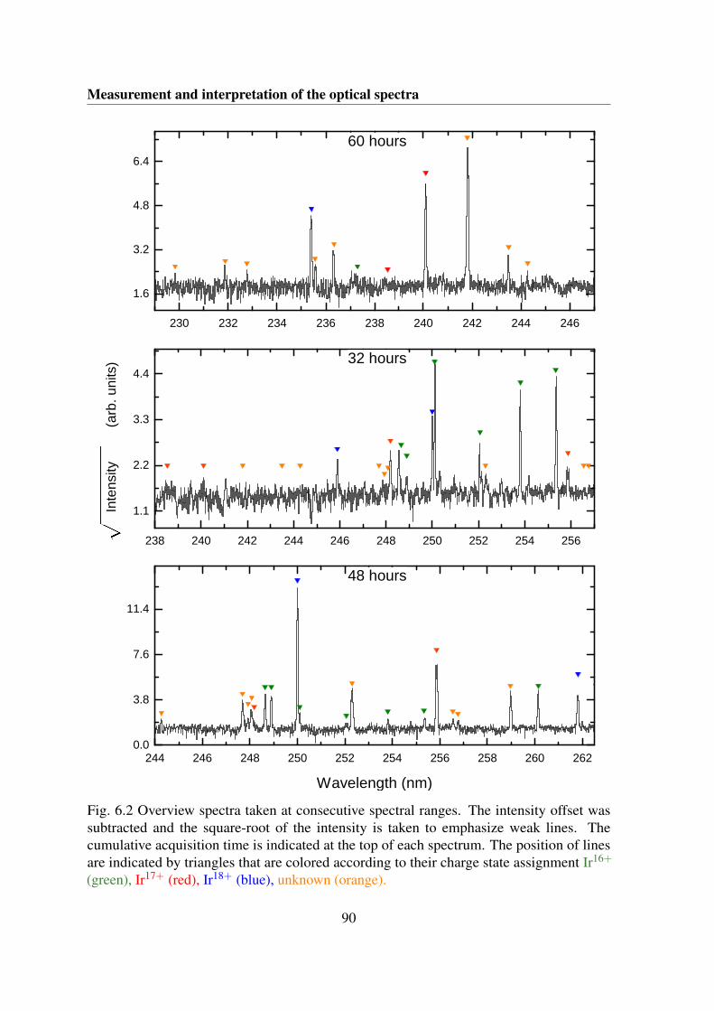
Measurement and interpretation of the optical spectra
2 3 0 2 3 2 2 3 4 2 3 6 2 3 8 2 4 0 2 4 2 2 4 4 2 4 6
1 . 6
3 . 2
4 . 8
6 . 4
2 3 8 2 4 0 2 4 2 2 4 4 2 4 6 2 4 8 2 5 0 2 5 2 2 5 4 2 5 6
1 . 1
2 . 2
3 . 3
4 . 4
2 4 4 2 4 6 2 4 8 2 5 0 2 5 2 2 5 4 2 5 6 2 5 8 2 6 0 2 6 20 . 0
3 . 8
7 . 6
1 1 . 4
4 8 h o u r s
6 0 h o u r s
Inte
nsity
(a
rb. u
nits
) 3 2 h o u r s
W a v e l e n g t h ( n m )
Fig. 6.2 Overview spectra taken at consecutive spectral ranges. The intensity offset wassubtracted and the square-root of the intensity is taken to emphasize weak lines. Thecumulative acquisition time is indicated at the top of each spectrum. The position of linesare indicated by triangles that are colored according to their charge state assignment Ir16+
(green), Ir17+ (red), Ir18+ (blue), unknown (orange).
90
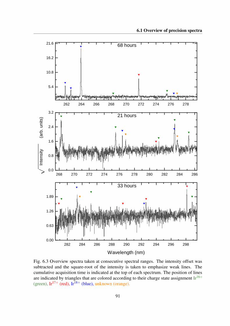
6.1 Overview of precision spectra
2 6 2 2 6 4 2 6 6 2 6 8 2 7 0 2 7 2 2 7 4 2 7 6 2 7 8
5 . 4
1 0 . 8
1 6 . 2
2 1 . 6
2 6 8 2 7 0 2 7 2 2 7 4 2 7 6 2 7 8 2 8 0 2 8 2 2 8 4 2 8 60 . 0
0 . 8
1 . 6
2 . 4
3 . 2
2 8 2 2 8 4 2 8 6 2 8 8 2 9 0 2 9 2 2 9 4 2 9 6 2 9 80 . 0 0
0 . 6 3
1 . 2 6
1 . 8 9
3 3 h o u r s
2 1 h o u r s
6 8 h o u r sIn
tens
ity
(arb
. uni
ts)
W a v e l e n g t h ( n m )
Fig. 6.3 Overview spectra taken at consecutive spectral ranges. The intensity offset wassubtracted and the square-root of the intensity is taken to emphasize weak lines. Thecumulative acquisition time is indicated at the top of each spectrum. The position of linesare indicated by triangles that are colored according to their charge state assignment Ir16+
(green), Ir17+ (red), Ir18+ (blue), unknown (orange).
91
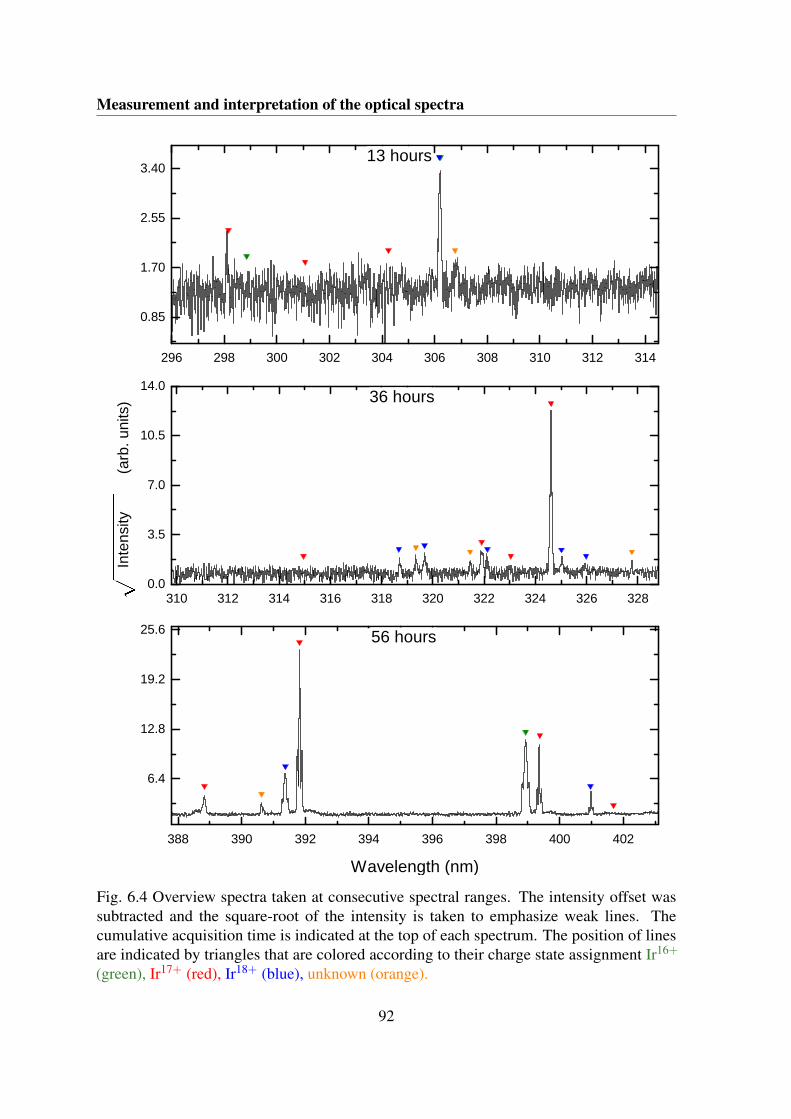
Measurement and interpretation of the optical spectra
2 9 6 2 9 8 3 0 0 3 0 2 3 0 4 3 0 6 3 0 8 3 1 0 3 1 2 3 1 4
0 . 8 5
1 . 7 0
2 . 5 5
3 . 4 0
3 1 0 3 1 2 3 1 4 3 1 6 3 1 8 3 2 0 3 2 2 3 2 4 3 2 6 3 2 80 . 0
3 . 5
7 . 0
1 0 . 5
1 4 . 0
3 8 8 3 9 0 3 9 2 3 9 4 3 9 6 3 9 8 4 0 0 4 0 2
6 . 4
1 2 . 8
1 9 . 2
2 5 . 6
3 6 h o u r s
1 3 h o u r s
Inte
nsity
(a
rb. u
nits
)
5 6 h o u r s
W a v e l e n g t h ( n m )
Fig. 6.4 Overview spectra taken at consecutive spectral ranges. The intensity offset wassubtracted and the square-root of the intensity is taken to emphasize weak lines. Thecumulative acquisition time is indicated at the top of each spectrum. The position of linesare indicated by triangles that are colored according to their charge state assignment Ir16+
(green), Ir17+ (red), Ir18+ (blue), unknown (orange).
92
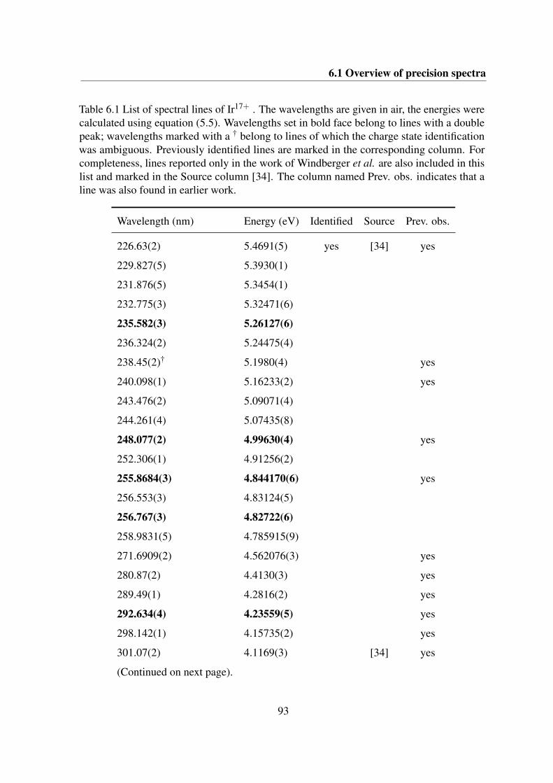
6.1 Overview of precision spectra
Table 6.1 List of spectral lines of Ir17+ . The wavelengths are given in air, the energies werecalculated using equation (5.5). Wavelengths set in bold face belong to lines with a doublepeak; wavelengths marked with a † belong to lines of which the charge state identificationwas ambiguous. Previously identified lines are marked in the corresponding column. Forcompleteness, lines reported only in the work of Windberger et al. are also included in thislist and marked in the Source column [34]. The column named Prev. obs. indicates that aline was also found in earlier work.
Wavelength (nm) Energy (eV) Identified Source Prev. obs.
226.63(2) 5.4691(5) yes [34] yes
229.827(5) 5.3930(1)
231.876(5) 5.3454(1)
232.775(3) 5.32471(6)
235.582(3) 5.26127(6)
236.324(2) 5.24475(4)
238.45(2)† 5.1980(4) yes
240.098(1) 5.16233(2) yes
243.476(2) 5.09071(4)
244.261(4) 5.07435(8)
248.077(2) 4.99630(4) yes
252.306(1) 4.91256(2)
255.8684(3) 4.844170(6) yes
256.553(3) 4.83124(5)
256.767(3) 4.82722(6)
258.9831(5) 4.785915(9)
271.6909(2) 4.562076(3) yes
280.87(2) 4.4130(3) yes
289.49(1) 4.2816(2) yes
292.634(4) 4.23559(5) yes
298.142(1) 4.15735(2) yes
301.07(2) 4.1169(3) [34] yes
(Continued on next page).
93
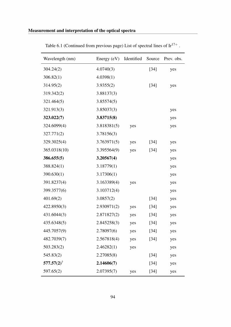
Measurement and interpretation of the optical spectra
Table 6.1 (Continued from previous page) List of spectral lines of Ir17+ .
Wavelength (nm) Energy (eV) Identified Source Prev. obs.
304.24(2) 4.0740(3) [34] yes
306.82(1) 4.0398(1)
314.95(2) 3.9355(2) [34] yes
319.342(2) 3.88137(3)
321.464(5) 3.85574(5)
321.913(3) 3.85037(3) yes
323.022(7) 3.83715(8) yes
324.6099(4) 3.818381(5) yes yes
327.771(2) 3.78156(3)
329.3025(4) 3.763971(5) yes [34] yes
365.0318(10) 3.395564(9) yes [34] yes
386.655(5) 3.20567(4) yes
388.824(1) 3.18779(1) yes
390.630(1) 3.17306(1) yes
391.8237(4) 3.163389(4) yes yes
399.3577(6) 3.103712(4) yes
401.69(2) 3.0857(2) [34] yes
422.8950(3) 2.930971(2) yes [34] yes
431.6044(3) 2.871827(2) yes [34] yes
435.6348(5) 2.845258(3) yes [34] yes
445.7057(9) 2.78097(6) yes [34] yes
482.7039(7) 2.567818(4) yes [34] yes
503.283(2) 2.46282(1) yes yes
545.83(2) 2.27085(8) [34] yes
577.57(2)† 2.14606(7) [34] yes
597.65(2) 2.07395(7) yes [34] yes
94
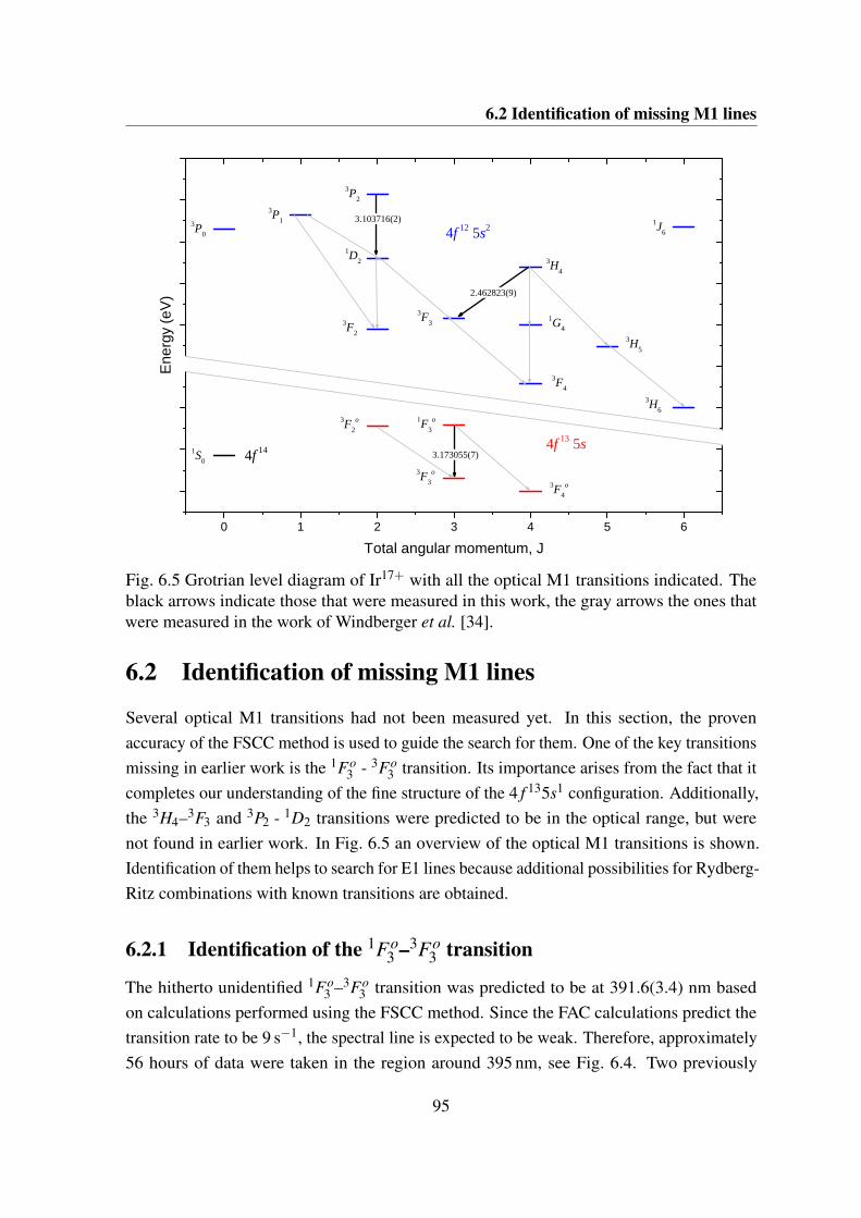
6.2 Identification of missing M1 lines
0 1 2 3 4 5 6
4 f 1 2 5 s 2
4 f 1 3 5 s
Ene
rgy
(eV
)
T o t a l a n g u l a r m o m e n t u m , J
1 S 0
3 P 23 P 13 P 0
1 J 6
1 D 2 3 H 4
1 G 4
3 F 33 F 2
3 F 4
3 H 5
3 H 61 F 3
o3 F 2o
3 F 3o
3 F 4o
3 . 1 0 3 7 1 6 ( 2 )
4 f 1 4
2 . 4 6 2 8 2 3 ( 9 )
3 . 1 7 3 0 5 5 ( 7 )
Fig. 6.5 Grotrian level diagram of Ir17+ with all the optical M1 transitions indicated. Theblack arrows indicate those that were measured in this work, the gray arrows the ones thatwere measured in the work of Windberger et al. [34].
6.2 Identification of missing M1 lines
Several optical M1 transitions had not been measured yet. In this section, the provenaccuracy of the FSCC method is used to guide the search for them. One of the key transitionsmissing in earlier work is the 1Fo
3 - 3Fo3 transition. Its importance arises from the fact that it
completes our understanding of the fine structure of the 4 f 135s1 configuration. Additionally,the 3H4–3F3 and 3P2 - 1D2 transitions were predicted to be in the optical range, but werenot found in earlier work. In Fig. 6.5 an overview of the optical M1 transitions is shown.Identification of them helps to search for E1 lines because additional possibilities for Rydberg-Ritz combinations with known transitions are obtained.
6.2.1 Identification of the 1Fo3 –3Fo
3 transition
The hitherto unidentified 1Fo3 –3Fo
3 transition was predicted to be at 391.6(3.4) nm basedon calculations performed using the FSCC method. Since the FAC calculations predict thetransition rate to be 9 s−1, the spectral line is expected to be weak. Therefore, approximately56 hours of data were taken in the region around 395 nm, see Fig. 6.4. Two previously
95
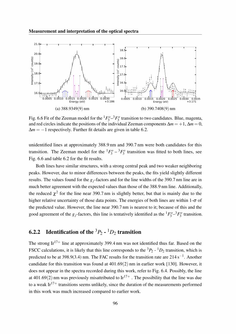
Measurement and interpretation of the optical spectra
0.0005 0.0010 0.0015 0.0020 0.0025 0.0030Energy (eV) +3.186
16.0
17.0
18.0
19.0
20.0
21.0
Inte
nsi
ty (
10
4 c
ounts
)
(a) 388.9349(9) nm
0.0005 0.0010 0.0015 0.0020 0.0025 0.0030 0.0035Energy (eV) +3.171
16.0
16.5
17.0
17.5
18.0
18.5
Inte
nsi
ty (
10
4 c
ounts
)
(b) 390.7408(9) nm
Fig. 6.6 Fit of the Zeeman model for the 1Fo3 –3Fo
3 transition to two candidates. Blue, magenta,and red circles indicate the positions of the individual Zeeman components ∆m=+1, ∆m= 0,∆m =−1 respectively. Further fit details are given in table 6.2.
unidentified lines at approximately 388.9 nm and 390.7 nm were both candidates for thistransition. The Zeeman model for the 1Fo
3 – 3Fo3 transition was fitted to both lines, see
Fig. 6.6 and table 6.2 for the fit results.
Both lines have similar structures, with a strong central peak and two weaker neighboringpeaks. However, due to minor differences between the peaks, the fits yield slightly differentresults. The values found for the g j-factors and for the line widths of the 390.7 nm line are inmuch better agreement with the expected values than those of the 388.9 nm line. Additionally,the reduced χ2 for the line near 390.7 nm is slightly better, but that is mainly due to thehigher relative uncertainty of those data points. The energies of both lines are within 1-σ ofthe predicted value. However, the line near 390.7 nm is nearest to it; because of this and thegood agreement of the g j-factors, this line is tentatively identified as the 1Fo
3 –3Fo3 transition.
6.2.2 Identification of the 3P2 - 1D2 transition
The strong Ir17+ line at approximately 399.4 nm was not identified thus far. Based on theFSCC calculations, it is likely that this line corresponds to the 3P2 - 1D2 transition, which ispredicted to be at 398.9(3.4) nm. The FAC results for the transition rate are 214 s−1. Anothercandidate for this transition was found at 401.69(2) nm in earlier work [130]. However, itdoes not appear in the spectra recorded during this work, refer to Fig. 6.4. Possibly, the lineat 401.69(2) nm was previously misattributed to Ir17+ . The possibility that the line was dueto a weak Ir17+ transitions seems unlikely, since the duration of the measurements performedin this work was much increased compared to earlier work.
96
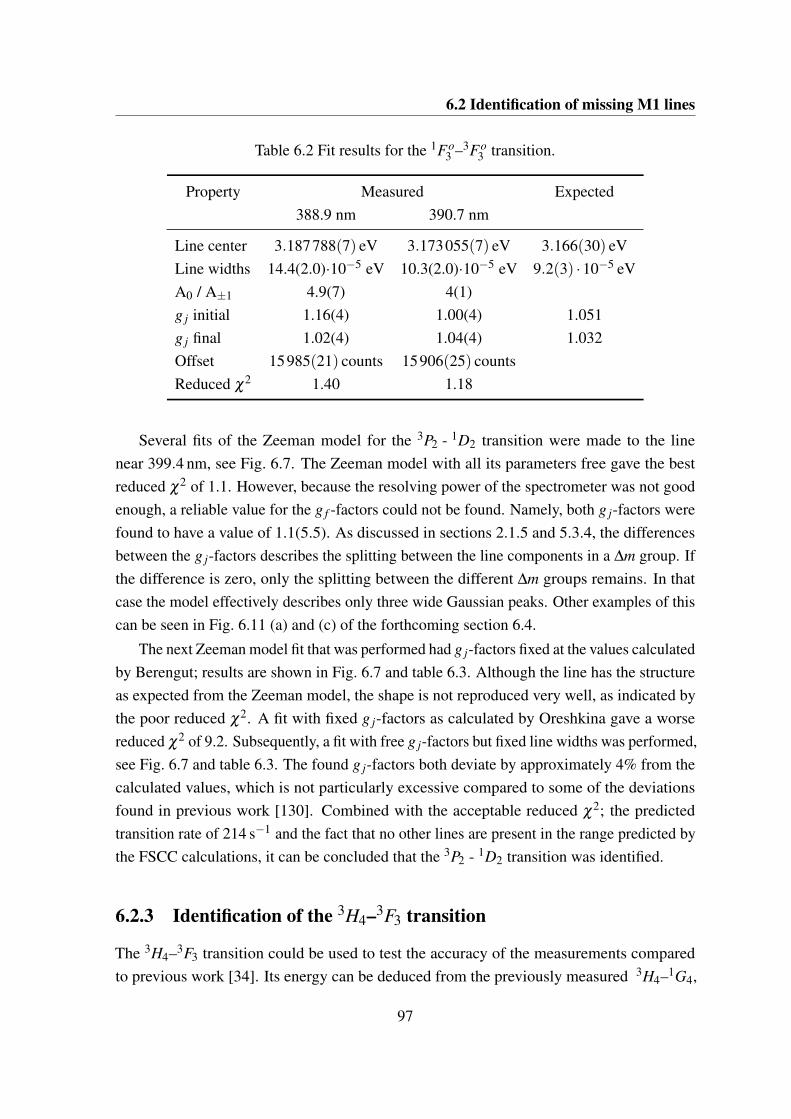
6.2 Identification of missing M1 lines
Table 6.2 Fit results for the 1Fo3 –3Fo
3 transition.
Property Measured Expected388.9 nm 390.7 nm
Line center 3.187788(7) eV 3.173055(7) eV 3.166(30) eVLine widths 14.4(2.0)·10−5 eV 10.3(2.0)·10−5 eV 9.2(3) ·10−5 eVA0 / A±1 4.9(7) 4(1)g j initial 1.16(4) 1.00(4) 1.051g j final 1.02(4) 1.04(4) 1.032Offset 15985(21) counts 15906(25) countsReduced χ2 1.40 1.18
Several fits of the Zeeman model for the 3P2 - 1D2 transition were made to the linenear 399.4 nm, see Fig. 6.7. The Zeeman model with all its parameters free gave the bestreduced χ2 of 1.1. However, because the resolving power of the spectrometer was not goodenough, a reliable value for the g f -factors could not be found. Namely, both g j-factors werefound to have a value of 1.1(5.5). As discussed in sections 2.1.5 and 5.3.4, the differencesbetween the g j-factors describes the splitting between the line components in a ∆m group. Ifthe difference is zero, only the splitting between the different ∆m groups remains. In thatcase the model effectively describes only three wide Gaussian peaks. Other examples of thiscan be seen in Fig. 6.11 (a) and (c) of the forthcoming section 6.4.
The next Zeeman model fit that was performed had g j-factors fixed at the values calculatedby Berengut; results are shown in Fig. 6.7 and table 6.3. Although the line has the structureas expected from the Zeeman model, the shape is not reproduced very well, as indicated bythe poor reduced χ2. A fit with fixed g j-factors as calculated by Oreshkina gave a worsereduced χ2 of 9.2. Subsequently, a fit with free g j-factors but fixed line widths was performed,see Fig. 6.7 and table 6.3. The found g j-factors both deviate by approximately 4% from thecalculated values, which is not particularly excessive compared to some of the deviationsfound in previous work [130]. Combined with the acceptable reduced χ2; the predictedtransition rate of 214 s−1 and the fact that no other lines are present in the range predicted bythe FSCC calculations, it can be concluded that the 3P2 - 1D2 transition was identified.
6.2.3 Identification of the 3H4–3F3 transition
The 3H4–3F3 transition could be used to test the accuracy of the measurements comparedto previous work [34]. Its energy can be deduced from the previously measured 3H4–1G4,
97
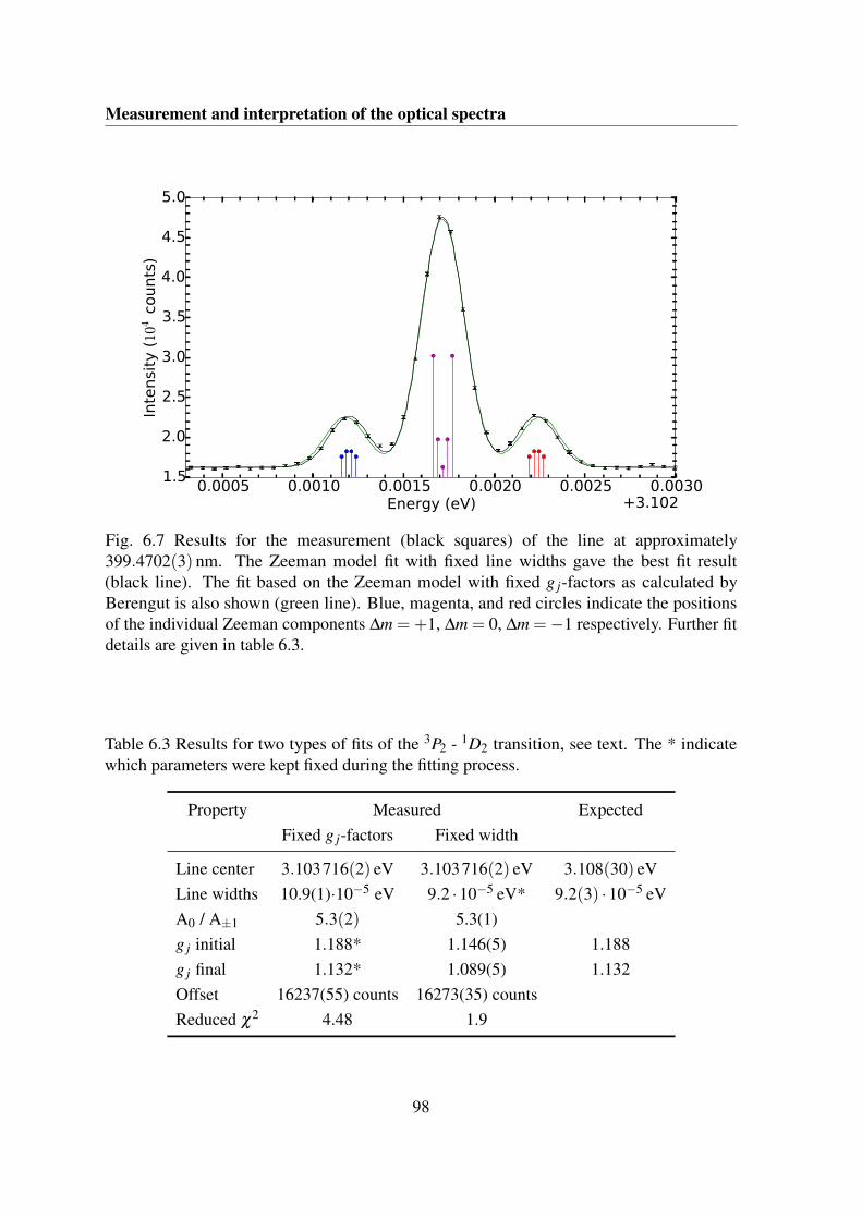
Measurement and interpretation of the optical spectra
0.0005 0.0010 0.0015 0.0020 0.0025 0.0030Energy (eV) +3.102
1.5
2.0
2.5
3.0
3.5
4.0
4.5
5.0
Inte
nsi
ty (
104
counts
)
Fig. 6.7 Results for the measurement (black squares) of the line at approximately399.4702(3) nm. The Zeeman model fit with fixed line widths gave the best fit result(black line). The fit based on the Zeeman model with fixed g j-factors as calculated byBerengut is also shown (green line). Blue, magenta, and red circles indicate the positionsof the individual Zeeman components ∆m =+1, ∆m = 0, ∆m =−1 respectively. Further fitdetails are given in table 6.3.
Table 6.3 Results for two types of fits of the 3P2 - 1D2 transition, see text. The * indicatewhich parameters were kept fixed during the fitting process.
Property Measured ExpectedFixed g j-factors Fixed width
Line center 3.103716(2) eV 3.103716(2) eV 3.108(30) eVLine widths 10.9(1)·10−5 eV 9.2 ·10−5 eV* 9.2(3) ·10−5 eVA0 / A±1 5.3(2) 5.3(1)g j initial 1.188* 1.146(5) 1.188g j final 1.132* 1.089(5) 1.132Offset 16237(55) counts 16273(35) countsReduced χ2 4.48 1.9
98
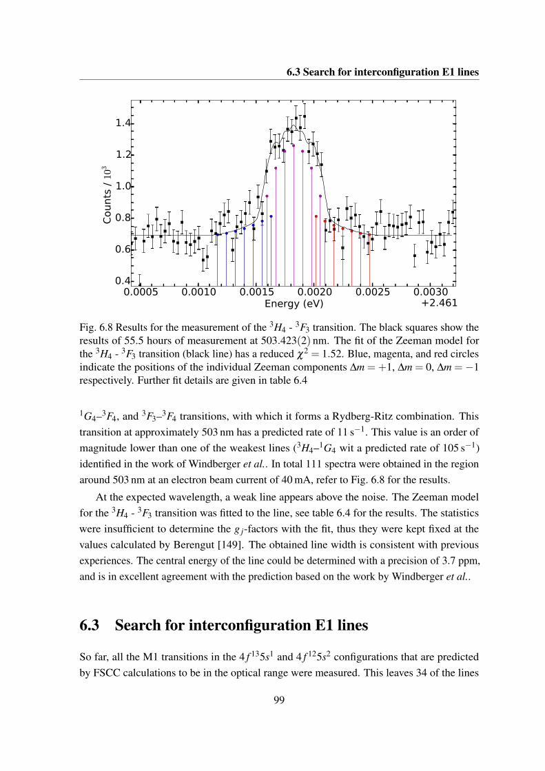
6.3 Search for interconfiguration E1 lines
0.0005 0.0010 0.0015 0.0020 0.0025 0.0030Energy (eV) +2.461
0.4
0.6
0.8
1.0
1.2
1.4
Counts
/ 1
03
Fig. 6.8 Results for the measurement of the 3H4 - 3F3 transition. The black squares show theresults of 55.5 hours of measurement at 503.423(2) nm. The fit of the Zeeman model forthe 3H4 - 3F3 transition (black line) has a reduced χ2 = 1.52. Blue, magenta, and red circlesindicate the positions of the individual Zeeman components ∆m =+1, ∆m = 0, ∆m =−1respectively. Further fit details are given in table 6.4
1G4–3F4, and 3F3–3F4 transitions, with which it forms a Rydberg-Ritz combination. Thistransition at approximately 503 nm has a predicted rate of 11 s−1. This value is an order ofmagnitude lower than one of the weakest lines (3H4–1G4 wit a predicted rate of 105 s−1)identified in the work of Windberger et al.. In total 111 spectra were obtained in the regionaround 503 nm at an electron beam current of 40 mA, refer to Fig. 6.8 for the results.
At the expected wavelength, a weak line appears above the noise. The Zeeman modelfor the 3H4 - 3F3 transition was fitted to the line, see table 6.4 for the results. The statisticswere insufficient to determine the g j-factors with the fit, thus they were kept fixed at thevalues calculated by Berengut [149]. The obtained line width is consistent with previousexperiences. The central energy of the line could be determined with a precision of 3.7 ppm,and is in excellent agreement with the prediction based on the work by Windberger et al..
6.3 Search for interconfiguration E1 lines
So far, all the M1 transitions in the 4 f 135s1 and 4 f 125s2 configurations that are predictedby FSCC calculations to be in the optical range were measured. This leaves 34 of the lines
99
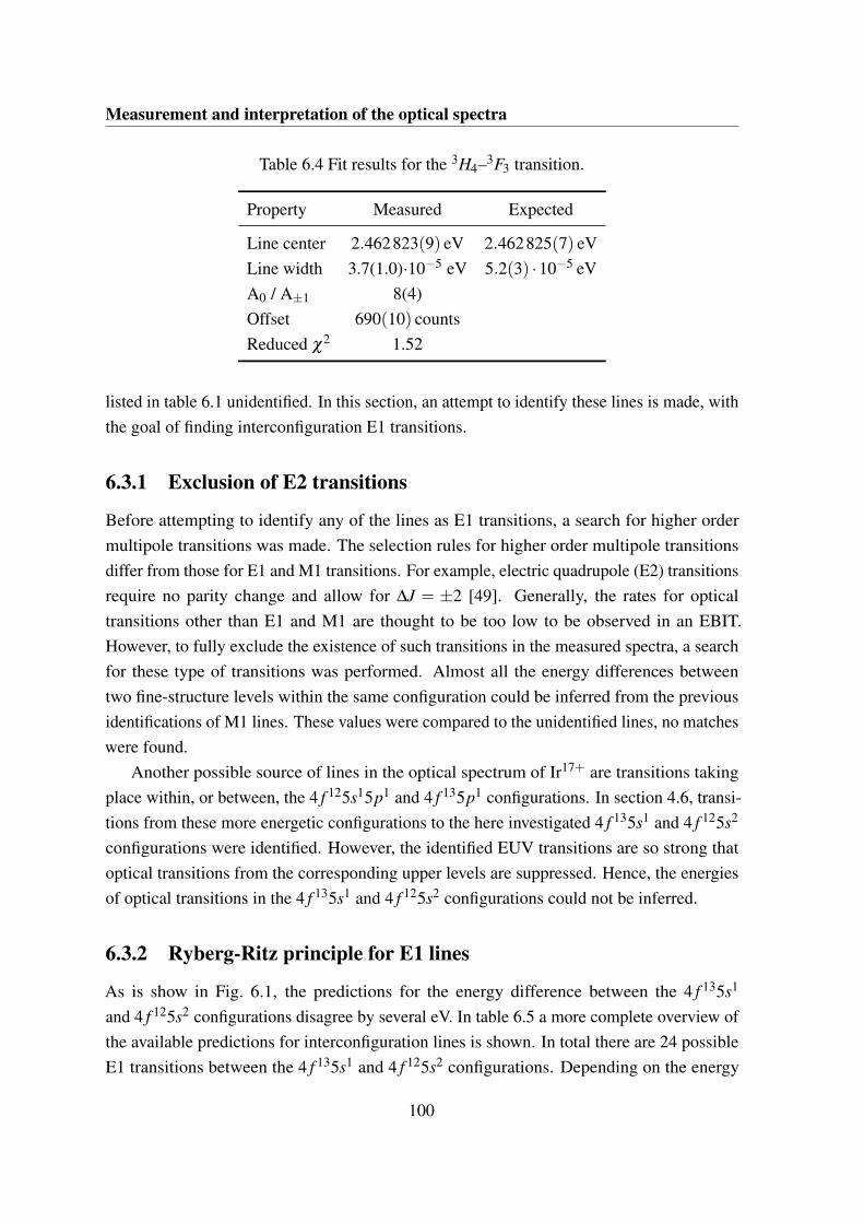
Measurement and interpretation of the optical spectra
Table 6.4 Fit results for the 3H4–3F3 transition.
Property Measured Expected
Line center 2.462823(9) eV 2.462825(7) eVLine width 3.7(1.0)·10−5 eV 5.2(3) ·10−5 eVA0 / A±1 8(4)Offset 690(10) countsReduced χ2 1.52
listed in table 6.1 unidentified. In this section, an attempt to identify these lines is made, withthe goal of finding interconfiguration E1 transitions.
6.3.1 Exclusion of E2 transitions
Before attempting to identify any of the lines as E1 transitions, a search for higher ordermultipole transitions was made. The selection rules for higher order multipole transitionsdiffer from those for E1 and M1 transitions. For example, electric quadrupole (E2) transitionsrequire no parity change and allow for ∆J = ±2 [49]. Generally, the rates for opticaltransitions other than E1 and M1 are thought to be too low to be observed in an EBIT.However, to fully exclude the existence of such transitions in the measured spectra, a searchfor these type of transitions was performed. Almost all the energy differences betweentwo fine-structure levels within the same configuration could be inferred from the previousidentifications of M1 lines. These values were compared to the unidentified lines, no matcheswere found.
Another possible source of lines in the optical spectrum of Ir17+ are transitions takingplace within, or between, the 4 f 125s15p1 and 4 f 135p1 configurations. In section 4.6, transi-tions from these more energetic configurations to the here investigated 4 f 135s1 and 4 f 125s2
configurations were identified. However, the identified EUV transitions are so strong thatoptical transitions from the corresponding upper levels are suppressed. Hence, the energiesof optical transitions in the 4 f 135s1 and 4 f 125s2 configurations could not be inferred.
6.3.2 Ryberg-Ritz principle for E1 lines
As is show in Fig. 6.1, the predictions for the energy difference between the 4 f 135s1
and 4 f 125s2 configurations disagree by several eV. In table 6.5 a more complete overview ofthe available predictions for interconfiguration lines is shown. In total there are 24 possibleE1 transitions between the 4 f 135s1 and 4 f 125s2 configurations. Depending on the energy
100
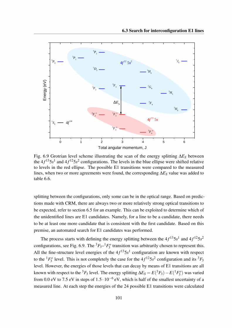
6.3 Search for interconfiguration E1 lines
0 1 2 3 4 5 6
4 f 1 2 5 s 2
4 f 1 3 5 s
Ene
rgy
(eV
)
T o t a l a n g u l a r m o m e n t u m , J
1 S 0
3 P 23 P 13 P 0
1 J 6
1 D 2 3 H 4
1 G 4
3 F 33 F 2
3 F 4
3 H 5
3 H 61 F 3
o3 F 2o
3 F 3o
3 F 4o
4 f 1 4
∆ E S
Fig. 6.9 Grotrian level scheme illustrating the scan of the energy splitting ∆ES betweenthe 4 f 135s1 and 4 f 125s2 configurations. The levels in the blue ellipse were shifted relativeto levels in the red ellipse. The possible E1 transitions were compared to the measuredlines, when two or more agreements were found, the corresponding ∆ES value was added totable 6.6.
splitting between the configurations, only some can be in the optical range. Based on predic-tions made with CRM, there are always two or more relatively strong optical transitions tobe expected, refer to section 6.5 for an example. This can be exploited to determine which ofthe unidentified lines are E1 candidates. Namely, for a line to be a candidate, there needsto be at least one more candidate that is consistent with the first candidate. Based on thispremise, an automated search for E1 candidates was performed.
The process starts with defining the energy splitting between the 4 f 135s1 and 4 f 125s2
configurations, see Fig. 6.9. The 3F3–1Fo3 transition was arbitrarily chosen to represent this.
All the fine-structure level energies of the 4 f 135s1 configuration are known with respectto the 1Fo
3 level. This is not completely the case for the 4 f 125s2 configuration and its 3F3
level. However, the energies of those levels that can decay by means of E1 transitions are allknown with respect to the 3F3 level. The energy splitting ∆ES = E(3F3)−E(1Fo
3 ) was variedfrom 0.0 eV to 7.5 eV in steps of 1.5 ·10−6 eV, which is half of the smallest uncertainty of ameasured line. At each step the energies of the 24 possible E1 transitions were calculated
101
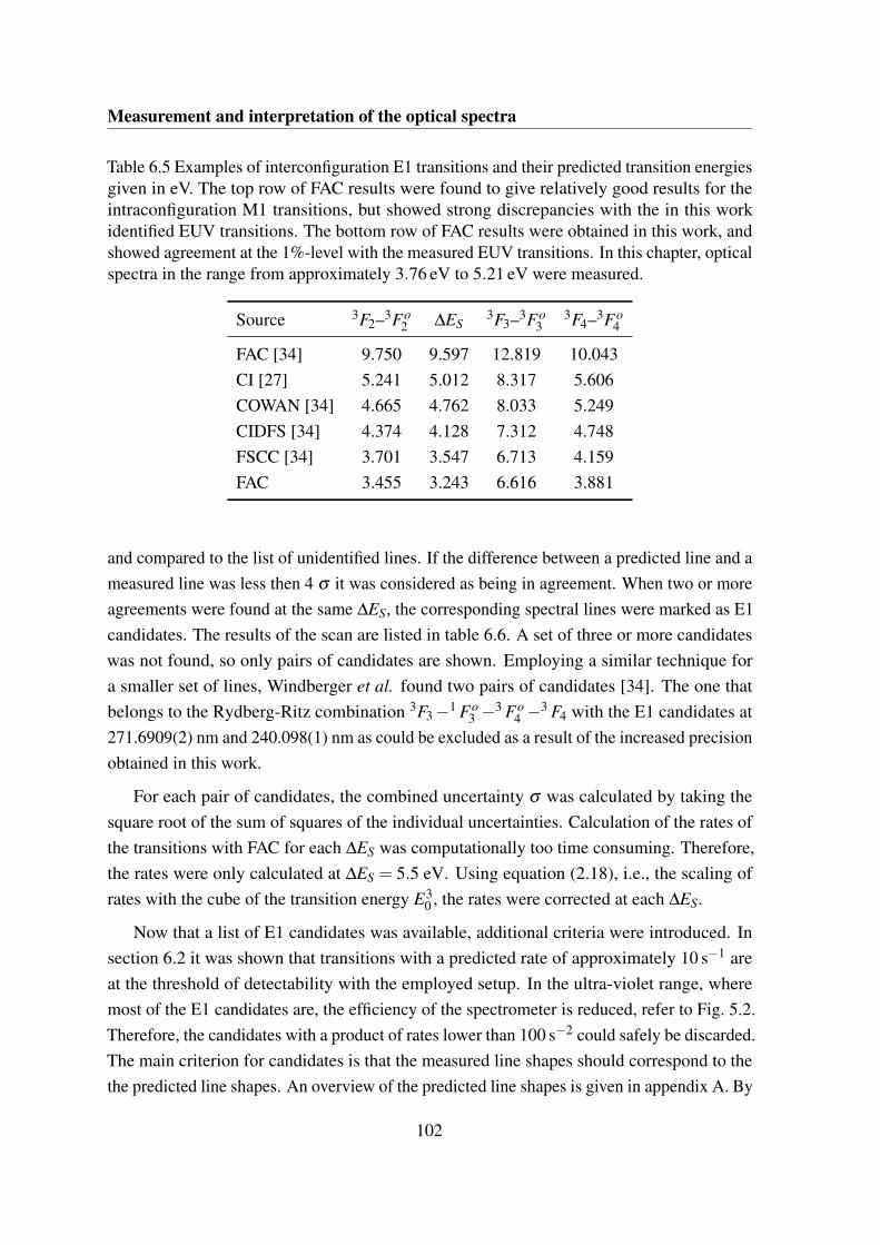
Measurement and interpretation of the optical spectra
Table 6.5 Examples of interconfiguration E1 transitions and their predicted transition energiesgiven in eV. The top row of FAC results were found to give relatively good results for theintraconfiguration M1 transitions, but showed strong discrepancies with the in this workidentified EUV transitions. The bottom row of FAC results were obtained in this work, andshowed agreement at the 1%-level with the measured EUV transitions. In this chapter, opticalspectra in the range from approximately 3.76 eV to 5.21 eV were measured.
Source 3F2–3Fo2 ∆ES
3F3–3Fo3
3F4–3Fo4
FAC [34] 9.750 9.597 12.819 10.043CI [27] 5.241 5.012 8.317 5.606COWAN [34] 4.665 4.762 8.033 5.249CIDFS [34] 4.374 4.128 7.312 4.748FSCC [34] 3.701 3.547 6.713 4.159FAC 3.455 3.243 6.616 3.881
and compared to the list of unidentified lines. If the difference between a predicted line and ameasured line was less then 4 σ it was considered as being in agreement. When two or moreagreements were found at the same ∆ES, the corresponding spectral lines were marked as E1candidates. The results of the scan are listed in table 6.6. A set of three or more candidateswas not found, so only pairs of candidates are shown. Employing a similar technique fora smaller set of lines, Windberger et al. found two pairs of candidates [34]. The one thatbelongs to the Rydberg-Ritz combination 3F3 −1 Fo
3 −3 Fo4 −3 F4 with the E1 candidates at
271.6909(2) nm and 240.098(1) nm as could be excluded as a result of the increased precisionobtained in this work.
For each pair of candidates, the combined uncertainty σ was calculated by taking thesquare root of the sum of squares of the individual uncertainties. Calculation of the rates ofthe transitions with FAC for each ∆ES was computationally too time consuming. Therefore,the rates were only calculated at ∆ES = 5.5 eV. Using equation (2.18), i.e., the scaling ofrates with the cube of the transition energy E3
0 , the rates were corrected at each ∆ES.
Now that a list of E1 candidates was available, additional criteria were introduced. Insection 6.2 it was shown that transitions with a predicted rate of approximately 10 s−1 areat the threshold of detectability with the employed setup. In the ultra-violet range, wheremost of the E1 candidates are, the efficiency of the spectrometer is reduced, refer to Fig. 5.2.Therefore, the candidates with a product of rates lower than 100 s−2 could safely be discarded.The main criterion for candidates is that the measured line shapes should correspond to thethe predicted line shapes. An overview of the predicted line shapes is given in appendix A. By
102
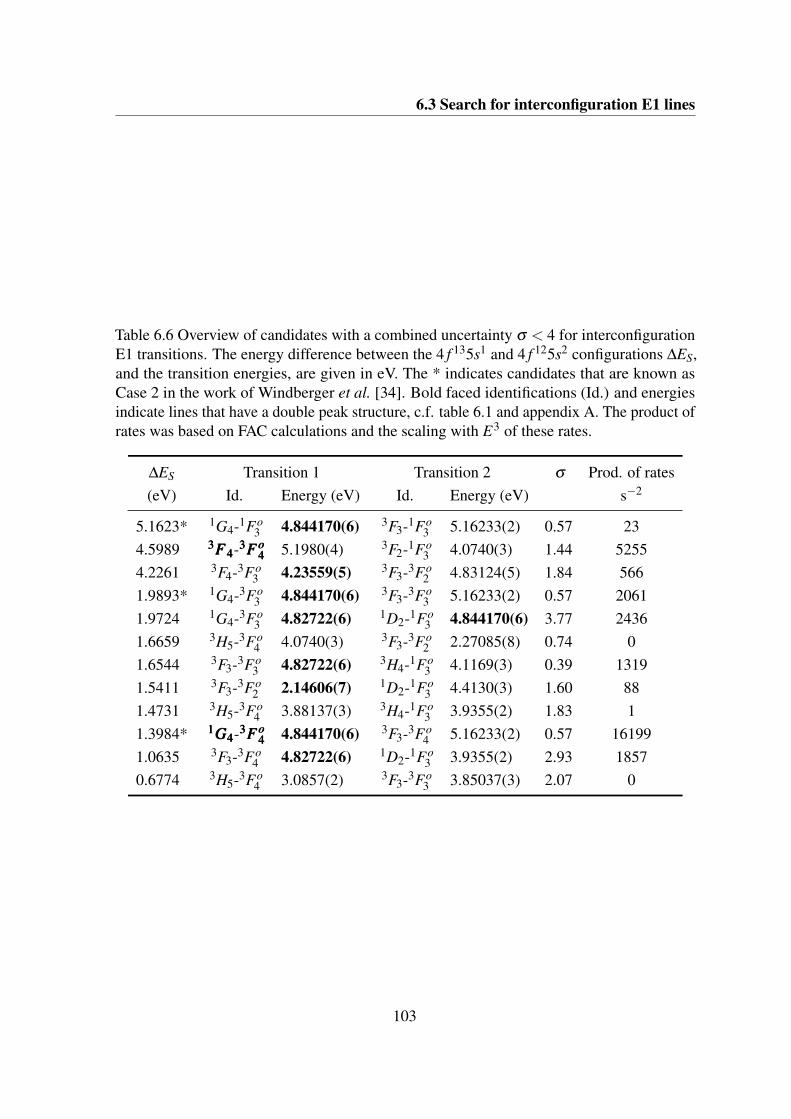
6.3 Search for interconfiguration E1 lines
Table 6.6 Overview of candidates with a combined uncertainty σ < 4 for interconfigurationE1 transitions. The energy difference between the 4 f 135s1 and 4 f 125s2 configurations ∆ES,and the transition energies, are given in eV. The * indicates candidates that are known asCase 2 in the work of Windberger et al. [34]. Bold faced identifications (Id.) and energiesindicate lines that have a double peak structure, c.f. table 6.1 and appendix A. The product ofrates was based on FAC calculations and the scaling with E3 of these rates.
∆ES Transition 1 Transition 2 σ Prod. of rates(eV) Id. Energy (eV) Id. Energy (eV) s−2
5.1623* 1G4-1Fo3 4.844170(6) 3F3-1Fo
3 5.16233(2) 0.57 234.5989 333FFF444-333FFFooo
444 5.1980(4) 3F2-1Fo3 4.0740(3) 1.44 5255
4.2261 3F4-3Fo3 4.23559(5) 3F3-3Fo
2 4.83124(5) 1.84 5661.9893* 1G4-3Fo
3 4.844170(6) 3F3-3Fo3 5.16233(2) 0.57 2061
1.9724 1G4-3Fo3 4.82722(6) 1D2-1Fo
3 4.844170(6) 3.77 24361.6659 3H5-3Fo
4 4.0740(3) 3F3-3Fo2 2.27085(8) 0.74 0
1.6544 3F3-3Fo3 4.82722(6) 3H4-1Fo
3 4.1169(3) 0.39 13191.5411 3F3-3Fo
2 2.14606(7) 1D2-1Fo3 4.4130(3) 1.60 88
1.4731 3H5-3Fo4 3.88137(3) 3H4-1Fo
3 3.9355(2) 1.83 11.3984* 111GGG444-333FFFooo
444 4.844170(6) 3F3-3Fo4 5.16233(2) 0.57 16199
1.0635 3F3-3Fo4 4.82722(6) 1D2-1Fo
3 3.9355(2) 2.93 18570.6774 3H5-3Fo
4 3.0857(2) 3F3-3Fo3 3.85037(3) 2.07 0
103
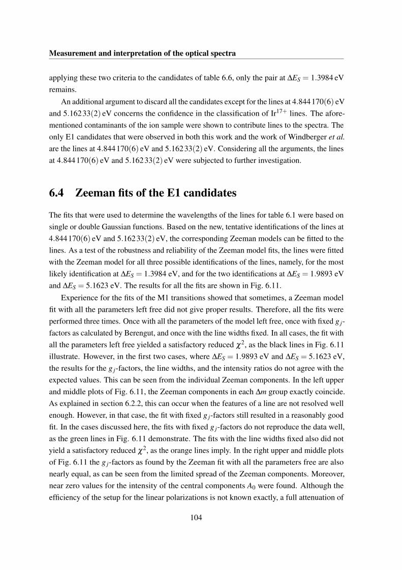
Measurement and interpretation of the optical spectra
applying these two criteria to the candidates of table 6.6, only the pair at ∆ES = 1.3984 eVremains.
An additional argument to discard all the candidates except for the lines at 4.844170(6) eVand 5.16233(2) eV concerns the confidence in the classification of Ir17+ lines. The afore-mentioned contaminants of the ion sample were shown to contribute lines to the spectra. Theonly E1 candidates that were observed in both this work and the work of Windberger et al.are the lines at 4.844170(6) eV and 5.16233(2) eV. Considering all the arguments, the linesat 4.844170(6) eV and 5.16233(2) eV were subjected to further investigation.
6.4 Zeeman fits of the E1 candidates
The fits that were used to determine the wavelengths of the lines for table 6.1 were based onsingle or double Gaussian functions. Based on the new, tentative identifications of the lines at4.844170(6) eV and 5.16233(2) eV, the corresponding Zeeman models can be fitted to thelines. As a test of the robustness and reliability of the Zeeman model fits, the lines were fittedwith the Zeeman model for all three possible identifications of the lines, namely, for the mostlikely identification at ∆ES = 1.3984 eV, and for the two identifications at ∆ES = 1.9893 eVand ∆ES = 5.1623 eV. The results for all the fits are shown in Fig. 6.11.
Experience for the fits of the M1 transitions showed that sometimes, a Zeeman modelfit with all the parameters left free did not give proper results. Therefore, all the fits wereperformed three times. Once with all the parameters of the model left free, once with fixed g j-factors as calculated by Berengut, and once with the line widths fixed. In all cases, the fit withall the parameters left free yielded a satisfactory reduced χ2, as the black lines in Fig. 6.11illustrate. However, in the first two cases, where ∆ES = 1.9893 eV and ∆ES = 5.1623 eV,the results for the g j-factors, the line widths, and the intensity ratios do not agree with theexpected values. This can be seen from the individual Zeeman components. In the left upperand middle plots of Fig. 6.11, the Zeeman components in each ∆m group exactly coincide.As explained in section 6.2.2, this can occur when the features of a line are not resolved wellenough. However, in that case, the fit with fixed g j-factors still resulted in a reasonably goodfit. In the cases discussed here, the fits with fixed g j-factors do not reproduce the data well,as the green lines in Fig. 6.11 demonstrate. The fits with the line widths fixed also did notyield a satisfactory reduced χ2, as the orange lines imply. In the right upper and middle plotsof Fig. 6.11 the g j-factors as found by the Zeeman fit with all the parameters free are alsonearly equal, as can be seen from the limited spread of the Zeeman components. Moreover,near zero values for the intensity of the central components A0 were found. Although theefficiency of the setup for the linear polarizations is not known exactly, a full attenuation of
104
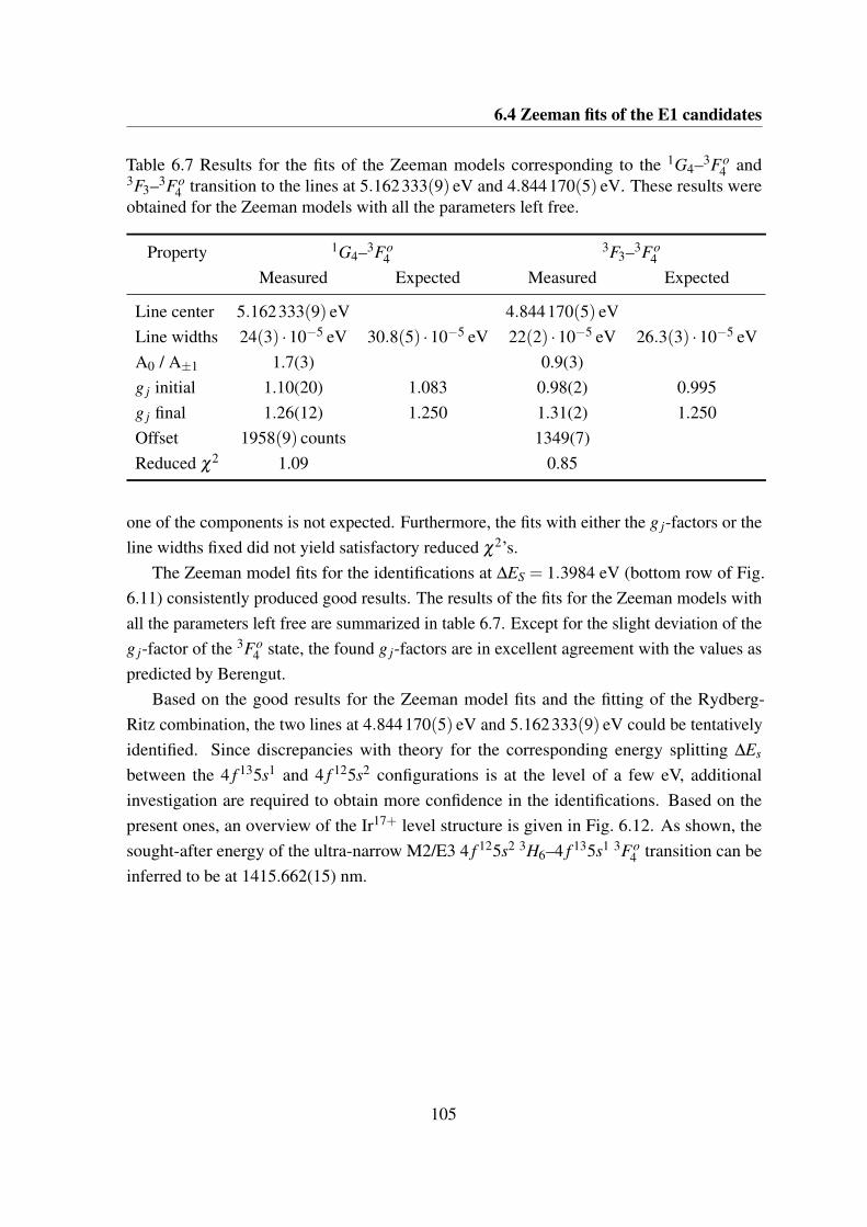
6.4 Zeeman fits of the E1 candidates
Table 6.7 Results for the fits of the Zeeman models corresponding to the 1G4–3Fo4 and
3F3–3Fo4 transition to the lines at 5.162333(9) eV and 4.844170(5) eV. These results were
obtained for the Zeeman models with all the parameters left free.
Property 1G4–3Fo4
3F3–3Fo4
Measured Expected Measured Expected
Line center 5.162333(9) eV 4.844170(5) eVLine widths 24(3) ·10−5 eV 30.8(5) ·10−5 eV 22(2) ·10−5 eV 26.3(3) ·10−5 eVA0 / A±1 1.7(3) 0.9(3)g j initial 1.10(20) 1.083 0.98(2) 0.995g j final 1.26(12) 1.250 1.31(2) 1.250Offset 1958(9) counts 1349(7)Reduced χ2 1.09 0.85
one of the components is not expected. Furthermore, the fits with either the g j-factors or theline widths fixed did not yield satisfactory reduced χ2’s.
The Zeeman model fits for the identifications at ∆ES = 1.3984 eV (bottom row of Fig.6.11) consistently produced good results. The results of the fits for the Zeeman models withall the parameters left free are summarized in table 6.7. Except for the slight deviation of theg j-factor of the 3Fo
4 state, the found g j-factors are in excellent agreement with the values aspredicted by Berengut.
Based on the good results for the Zeeman model fits and the fitting of the Rydberg-Ritz combination, the two lines at 4.844170(5) eV and 5.162333(9) eV could be tentativelyidentified. Since discrepancies with theory for the corresponding energy splitting ∆Es
between the 4 f 135s1 and 4 f 125s2 configurations is at the level of a few eV, additionalinvestigation are required to obtain more confidence in the identifications. Based on thepresent ones, an overview of the Ir17+ level structure is given in Fig. 6.12. As shown, thesought-after energy of the ultra-narrow M2/E3 4 f 125s2 3H6–4 f 135s1 3Fo
4 transition can beinferred to be at 1415.662(15) nm.
105
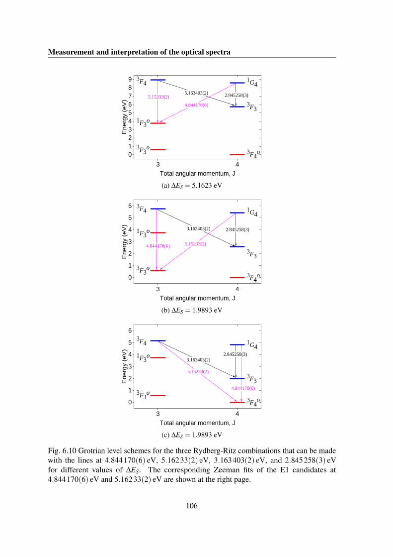
Measurement and interpretation of the optical spectra
3 40123456789
3 F 4o
3 F 4 1 G 4
3 F 3
1 F 3 o
3 F 3o
Ene
rgy
(eV
)
T o t a l a n g u l a r m o m e n t u m , J
3 . 1 6 3 4 0 3 ( 2 ) 2 . 8 4 5 2 5 8 ( 3 )5 . 1 5 2 3 3 ( 2 )4 . 8 4 4 1 7 0 ( 6 )
(a) ∆ES = 5.1623 eV
3 4
0
1
2
3
4
5
6
3 F 4o
3 F 4 1 G 4
3 F 3
1 F 3 o
3 F 3o
Ene
rgy
(eV
)
T o t a l a n g u l a r m o m e n t u m , J
3 . 1 6 3 4 0 3 ( 2 ) 2 . 8 4 5 2 5 8 ( 3 )
5 . 1 5 2 3 3 ( 2 )4 . 8 4 4 1 7 0 ( 6 )
(b) ∆ES = 1.9893 eV
3 4
0
1
2
3
4
5
6
3 F 4o
3 F 4 1 G 4
3 F 3
1 F 3 o
3 F 3o
Ene
rgy
(eV
)
T o t a l a n g u l a r m o m e n t u m , J
3 . 1 6 3 4 0 3 ( 2 )2 . 8 4 5 2 5 8 ( 3 )
5 . 1 5 2 3 3 ( 2 )
4 . 8 4 4 1 7 0 ( 6 )
(c) ∆ES = 1.9893 eV
Fig. 6.10 Grotrian level schemes for the three Rydberg-Ritz combinations that can be madewith the lines at 4.844170(6) eV, 5.16233(2) eV, 3.163403(2) eV, and 2.845258(3) eVfor different values of ∆ES. The corresponding Zeeman fits of the E1 candidates at4.844170(6) eV and 5.16233(2) eV are shown at the right page.
106
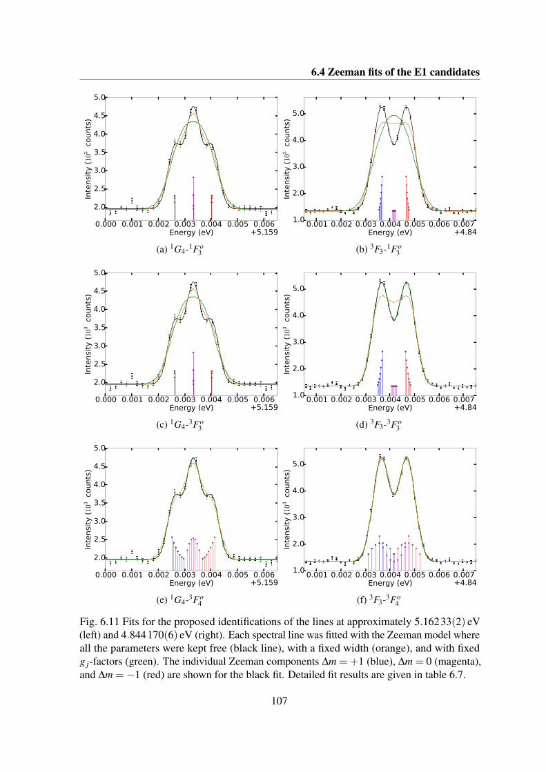
6.4 Zeeman fits of the E1 candidates
0.000 0.001 0.002 0.003 0.004 0.005 0.006Energy (eV) +5.159
2.0
2.5
3.0
3.5
4.0
4.5
5.0In
tensi
ty (
103
counts
)
(a) 1G4-1Fo3
0.001 0.002 0.003 0.004 0.005 0.006 0.007Energy (eV) +4.84
1.0
2.0
3.0
4.0
5.0
Inte
nsi
ty (
103
counts
)
(b) 3F3-1Fo3
0.000 0.001 0.002 0.003 0.004 0.005 0.006Energy (eV) +5.159
2.0
2.5
3.0
3.5
4.0
4.5
5.0
Inte
nsi
ty (
103
counts
)
(c) 1G4-3Fo3
0.001 0.002 0.003 0.004 0.005 0.006 0.007Energy (eV) +4.84
1.0
2.0
3.0
4.0
5.0In
tensi
ty (
103
counts
)
(d) 3F3-3Fo3
0.000 0.001 0.002 0.003 0.004 0.005 0.006Energy (eV) +5.159
2.0
2.5
3.0
3.5
4.0
4.5
5.0
Inte
nsi
ty (
10
3 c
ounts
)
(e) 1G4-3Fo4
0.001 0.002 0.003 0.004 0.005 0.006 0.007Energy (eV) +4.84
1.0
2.0
3.0
4.0
5.0
Inte
nsi
ty (
10
3 c
ounts
)
(f) 3F3-3Fo4
Fig. 6.11 Fits for the proposed identifications of the lines at approximately 5.16233(2) eV(left) and 4.844170(6) eV (right). Each spectral line was fitted with the Zeeman model whereall the parameters were kept free (black line), with a fixed width (orange), and with fixedg j-factors (green). The individual Zeeman components ∆m =+1 (blue), ∆m = 0 (magenta),and ∆m =−1 (red) are shown for the black fit. Detailed fit results are given in table 6.7.
107
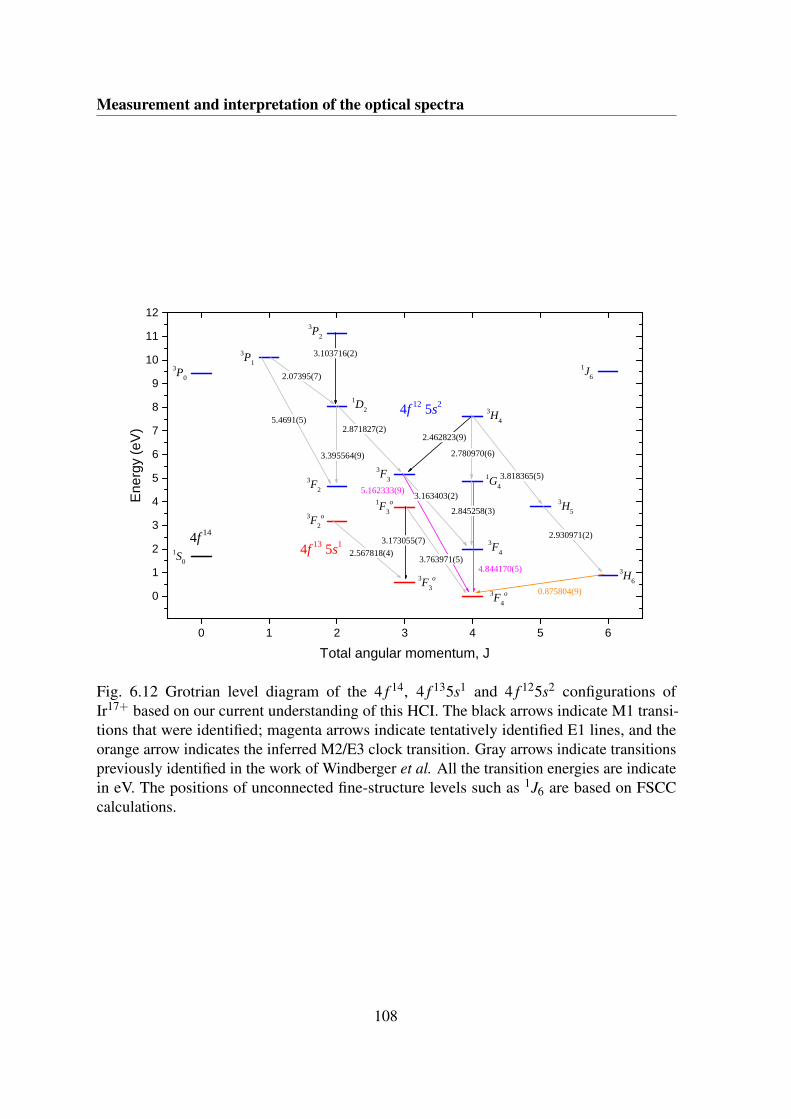
Measurement and interpretation of the optical spectra
0 1 2 3 4 5 6
0
1
2
3
4
5
6
7
8
9
1 0
1 1
1 2
0 . 8 7 5 8 0 4 ( 9 )
4 . 8 4 4 1 7 0 ( 5 )
5 . 1 6 2 3 3 3 ( 9 )
4 f 1 2 5 s 2
4 f 1 3 5 s 1
Ene
rgy
(eV
)
T o t a l a n g u l a r m o m e n t u m , J
1 S 0
3 P 2
3 P 13 P 0
1 J 6
1 D 2 3 H 4
1 G 4
3 F 33 F 2
3 F 4
3 H 5
3 H 6
1 F 3o
3 F 2o
3 F 3o
3 F 4o
3 . 1 6 3 4 0 3 ( 2 )
3 . 3 9 5 5 6 4 ( 9 )
3 . 7 6 3 9 7 1 ( 5 )
2 . 0 7 3 9 5 ( 7 )
5 . 4 6 9 1 ( 5 )2 . 8 7 1 8 2 7 ( 2 )
2 . 7 8 0 9 7 0 ( 6 )
2 . 8 4 5 2 5 8 ( 3 )
3 . 8 1 8 3 6 5 ( 5 )
2 . 9 3 0 9 7 1 ( 2 )
2 . 5 6 7 8 1 8 ( 4 )4 f 1 4
3 . 1 7 3 0 5 5 ( 7 )
2 . 4 6 2 8 2 3 ( 9 )
3 . 1 0 3 7 1 6 ( 2 )
Fig. 6.12 Grotrian level diagram of the 4 f 14, 4 f 135s1 and 4 f 125s2 configurations ofIr17+ based on our current understanding of this HCI. The black arrows indicate M1 transi-tions that were identified; magenta arrows indicate tentatively identified E1 lines, and theorange arrow indicates the inferred M2/E3 clock transition. Gray arrows indicate transitionspreviously identified in the work of Windberger et al. All the transition energies are indicatein eV. The positions of unconnected fine-structure levels such as 1J6 are based on FSCCcalculations.
108
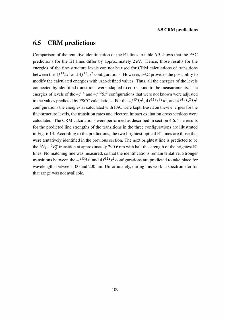
6.5 CRM predictions
6.5 CRM predictions
Comparison of the tentative identification of the E1 lines to table 6.5 shows that the FACpredictions for the E1 lines differ by approximately 2 eV. Hence, those results for theenergies of the fine-structure levels can not be used for CRM calculations of transitionsbetween the 4 f 135s1 and 4 f 125s2 configurations. However, FAC provides the possibility tomodify the calculated energies with user-defined values. Thus, all the energies of the levelsconnected by identified transitions were adapted to correspond to the measurements. Theenergies of levels of the 4 f 14 and 4 f 125s2 configurations that were not known were adjustedto the values predicted by FSCC calculations. For the 4 f 135p1, 4 f 125s15p1, and 4 f 115s25p1
configurations the energies as calculated with FAC were kept. Based on these energies for thefine-structure levels, the transition rates and electron impact excitation cross sections werecalculated. The CRM calculations were performed as described in section 4.6. The resultsfor the predicted line strengths of the transitions in the three configurations are illustratedin Fig. 6.13. According to the predictions, the two brightest optical E1 lines are those thatwere tentatively identified in the previous section. The next brightest line is predicted to bethe 1G4 – 3Fo
3 transition at approximately 290.6 nm with half the strength of the brightest E1lines. No matching line was measured, so that the identifications remain tentative. Strongertransitions between the 4 f 135s1 and 4 f 125s2 configurations are predicted to take place forwavelengths between 100 and 200 nm. Unfortunately, during this work, a spectrometer forthat range was not available.
109
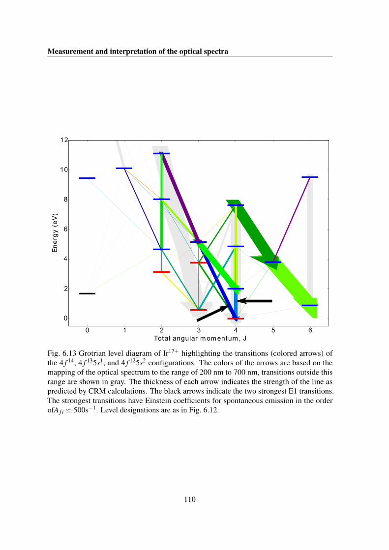
Measurement and interpretation of the optical spectra
0 1 2 3 4 5 6Total angular m om entum , J
0
2
4
6
8
10
12
En
erg
y (
eV
)
Fig. 6.13 Grotrian level diagram of Ir17+ highlighting the transitions (colored arrows) ofthe 4 f 14, 4 f 135s1, and 4 f 125s2 configurations. The colors of the arrows are based on themapping of the optical spectrum to the range of 200 nm to 700 nm, transitions outside thisrange are shown in gray. The thickness of each arrow indicates the strength of the line aspredicted by CRM calculations. The black arrows indicate the two strongest E1 transitions.The strongest transitions have Einstein coefficients for spontaneous emission in the orderofA f i ⋍ 500s−1. Level designations are as in Fig. 6.12.
110
Chapter 7
Summary and outlook
Currently, the most advanced frequency standards (clocks) based on a single ion reachfractional uncertainties at the level of ∆ν/ν0 ≈ 10−17. A large part of the uncertainty of thesedevices is due to the sensitivity of the energy levels of ions to external electric and magneticfields. Therefore, it was proposed to use transitions of highly charged ions (HCI) in frequencystandards. Due to their compact size, the sensitivity of HCI to external perturbations is highlysuppressed [35]. An abundance of suitable HCI has been proposed during recent years.In almost all of these, the required optical transitions exist as a result of level crossingsof two or more configurations [27, 36, 40]. The accuracy of predictions for the electronicstructure of these HCI is limited due to the intricate electron-electron correlations inherentto these complex many-electron systems. On the experimental side, measurements of thespectra of HCI near level crossings are lacking. Thus, the wavelengths of the HCI clocktransitions are not known to high enough precision for laser spectroscopy, a prerequisite forthe implementation as a frequency standard.
A prime application of frequency standards is the search for variations of fundamentalconstants. The single most stringent laboratory test of variation of constants up to date wasperformed on the fine-structure constant α . By measuring the ratio of the wavelengths oftwo transitions with different sensitivities to the variation of α several times over the courseof approximately a year, the variation was determined to be ∆α =−1.6(2.3)10−17/yr. Dueto increased relativistic effects, fine-structure energy levels of HCI can have an increasedsensitivity to ∆α . For electrons in nearly filled orbitals, such as near the 4 f –5s level crossing,these effects can be even more enhanced [27]. Hence, Nd-like Ir17+ has transitions thatbelong to the most ∆α-sensitive transitions predicted. Until recently, no spectroscopicdata was available for Ir17+ . The work by Windberger et al. changed that, 11 opticaltransitions of Ir17+ were identified [34]. These were all magnetic dipole (M1) transitions,taking place within a given configuration. Several of the measured yet unidentified lines
111
Summary and outlook
were suggested to be electric dipole (E1) transitions that take place between the 4 f 135s1 and4 f 125s2 configurations. These have the highest known sensitivity to ∆α in a stable atomicsystem, hence, knowledge of their wavelengths is imperative for the use of Ir17+ as a detectorof ∆α . Unfortunately, the uncertainties of the measured wavelengths precluded an ultimateidentification of the suggested lines.
Already in the year 1980, Curtis and Ellis made a theoretical study of the 4 f –5s levelcrossing [46]. They predicted that for Pm-like ions with atomic numbers Z ≥ 74 the electronicstructure is alkalilike, i.e. it consists of a single valence electron above closed shells. Thesesystems feature 5s–5p transitions in the extreme ultraviolet (EUV) range that were predictedto be prominent enough to be useful for plasma diagnostics. Despite considerable effortfrom several experimental groups to measure the predicted 5s–5p transitions, no definitiveidentifications had been made [119, 121, 122]. Many of the identifications were impeded bythe dense spectra and the uncertainties of predictions at the level of 1%.
In this work, Re, Os, Ir, and Pt (Z = 75−78) ions of the Pr-like, Nd-like, and Pm-likecharge states were experimentally investigated in the optical and EUV range. The HCI wereproduced and trapped in the Heidelberg electron beam ion trap (HD-EBIT). In an EBIT, themono-energetic electron beam ionizes atoms sequentially to the desired charge state, hence awell-defined charge-state distribution of the ions can be obtained. The electron beam excitesthe trapped HCI by electron impact. The subsequent fluorescence light was recorded by twospectrometers. With the EUV spectrometer spectra of Pr-like, Nd-like, and Pm-like Re, Os,Ir, and Pt were obtained. For the optical spectrometer procedures were developed to measureweak lines. These were applied to search and measure candidates for interconfigurationtransitions of Ir17+ .
Despite the predicted abundance of strong near-ground-state transitions of the Pm-likeions in the EUV regime, the measured spectra contained relatively few lines. To interpretthe EUV spectra, modeling of the electron-ion interactions in the EBIT proved necessary.The employed collisional radiative model (CRM) accounted for electron impact excitationand de-excitation, and for spontaneous decay of the fine-structure levels. By solving thequasi-stationary-state rate equations, the populations of the levels, and the line strengthsat the prevailing experimental conditions could be predicted. It was concluded that thespectrum was dominated by 4 f 135s15p1 – 4 f 135s2 transitions, leading to the identification ofseveral of these lines. The 4 f 125p1
3/2 – 4 f 125s1 transitions, although appearing weak, couldbe identified in Re14+, Os15+, Ir16+, and Pt17+. Comparison to several predictions basedon advanced configuration interaction and relativistic many-body perturbation calculationsshowed discrepancies at the level of 1% [123, 72]. Considering the low strength of the 5s–5p
112
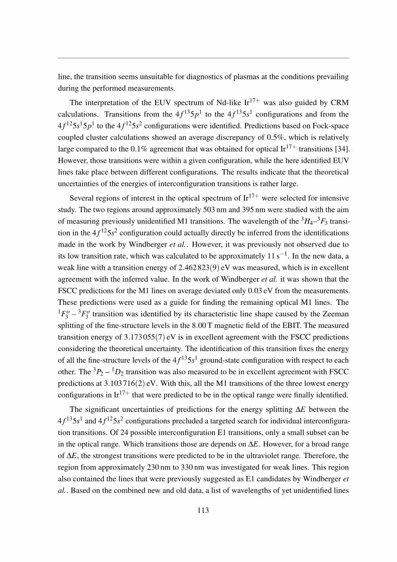
line, the transition seems unsuitable for diagnostics of plasmas at the conditions prevailingduring the performed measurements.
The interpretation of the EUV spectrum of Nd-like Ir17+ was also guided by CRMcalculations. Transitions from the 4 f 135p1 to the 4 f 135s1 configurations and from the4 f 125s15p1 to the 4 f 125s2 configurations were identified. Predictions based on Fock-spacecoupled cluster calculations showed an average discrepancy of 0.5%, which is relativelylarge compared to the 0.1% agreement that was obtained for optical Ir17+ transitions [34].However, those transitions were within a given configuration, while the here identified EUVlines take place between different configurations. The results indicate that the theoreticaluncertainties of the energies of interconfiguration transitions is rather large.
Several regions of interest in the optical spectrum of Ir17+ were selected for intensivestudy. The two regions around approximately 503 nm and 395 nm were studied with the aimof measuring previously unidentified M1 transitions. The wavelength of the 3H4–3F3 transi-tion in the 4 f 125s2 configuration could actually directly be inferred from the identificationsmade in the work by Windberger et al.. However, it was previously not observed due toits low transition rate, which was calculated to be approximately 11 s−1. In the new data, aweak line with a transition energy of 2.462823(9) eV was measured, which is in excellentagreement with the inferred value. In the work of Windberger et al. it was shown that theFSCC predictions for the M1 lines on average deviated only 0.03 eV from the measurements.These predictions were used as a guide for finding the remaining optical M1 lines. The1Fo
3 – 3Fo3 transition was identified by its characteristic line shape caused by the Zeeman
splitting of the fine-structure levels in the 8.00 T magnetic field of the EBIT. The measuredtransition energy of 3.173055(7) eV is in excellent agreement with the FSCC predictionsconsidering the theoretical uncertainty. The identification of this transition fixes the energyof all the fine-structure levels of the 4 f 135s1 ground-state configuration with respect to eachother. The 3P2 – 1D2 transition was also measured to be in excellent agreement with FSCCpredictions at 3.103716(2) eV. With this, all the M1 transitions of the three lowest energyconfigurations in Ir17+ that were predicted to be in the optical range were finally identified.
The significant uncertainties of predictions for the energy splitting ∆E between the4 f 135s1 and 4 f 125s2 configurations precluded a targeted search for individual interconfigura-tion transitions. Of 24 possible interconfiguration E1 transitions, only a small subset can bein the optical range. Which transitions those are depends on ∆E. However, for a broad rangeof ∆E, the strongest transitions were predicted to be in the ultraviolet range. Therefore, theregion from approximately 230 nm to 330 nm was investigated for weak lines. This regionalso contained the lines that were previously suggested as E1 candidates by Windberger etal.. Based on the combined new and old data, a list of wavelengths of yet unidentified lines
113
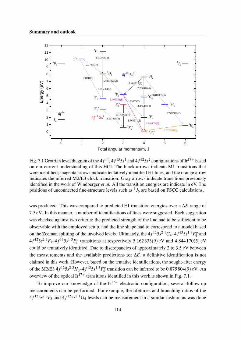
Summary and outlook
0 1 2 3 4 5 6
0
1
2
3
4
5
6
7
8
9
1 0
1 1
1 2
0 . 8 7 5 8 0 4 ( 9 )
4 . 8 4 4 1 7 0 ( 5 )
5 . 1 6 2 3 3 3 ( 9 )
4 f 1 2 5 s 2
4 f 1 3 5 s 1
Ene
rgy
(eV
)
T o t a l a n g u l a r m o m e n t u m , J
1 S 0
3 P 2
3 P 13 P 0
1 J 6
1 D 2 3 H 4
1 G 4
3 F 33 F 2
3 F 4
3 H 5
3 H 6
1 F 3o
3 F 2o
3 F 3o
3 F 4o
3 . 1 6 3 4 0 3 ( 2 )
3 . 3 9 5 5 6 4 ( 9 )
3 . 7 6 3 9 7 1 ( 5 )
2 . 0 7 3 9 5 ( 7 )
5 . 4 6 9 1 ( 5 )2 . 8 7 1 8 2 7 ( 2 )
2 . 7 8 0 9 7 0 ( 6 )
2 . 8 4 5 2 5 8 ( 3 )
3 . 8 1 8 3 6 5 ( 5 )
2 . 9 3 0 9 7 1 ( 2 )
2 . 5 6 7 8 1 8 ( 4 )4 f 1 4
3 . 1 7 3 0 5 5 ( 7 )
2 . 4 6 2 8 2 3 ( 9 )
3 . 1 0 3 7 1 6 ( 2 )
Fig. 7.1 Grotrian level diagram of the 4 f 14, 4 f 135s1 and 4 f 125s2 configurations of Ir17+ basedon our current understanding of this HCI. The black arrows indicate M1 transitions thatwere identified; magenta arrows indicate tentatively identified E1 lines, and the orange arrowindicates the inferred M2/E3 clock transition. Gray arrows indicate transitions previouslyidentified in the work of Windberger et al. All the transition energies are indicate in eV. Thepositions of unconnected fine-structure levels such as 1J6 are based on FSCC calculations.
was produced. This was compared to predicted E1 transition energies over a ∆E range of7.5 eV. In this manner, a number of identifications of lines were suggested. Each suggestionwas checked against two criteria: the predicted strength of the line had to be sufficient to beobservable with the employed setup, and the line shape had to correspond to a model basedon the Zeeman splitting of the involved levels. Ultimately, the 4 f 125s2 1G4–4 f 135s1 3Fo
4 and4 f 125s2 3F3–4 f 135s1 3Fo
4 transitions at respectively 5.162333(9) eV and 4.844170(5) eVcould be tentatively identified. Due to discrepancies of approximately 2 to 3.5 eV betweenthe measurements and the available predictions for ∆E, a definitive identification is notclaimed in this work. However, based on the tentative identifications, the sought-after energyof the M2/E3 4 f 125s2 3H6–4 f 135s1 3Fo
4 transition can be inferred to be 0.875804(9) eV. Anoverview of the optical Ir17+ transitions identified in this work is shown in Fig. 7.1.
To improve our knowledge of the Ir17+ electronic configuration, several follow-upmeasurements can be performed. For example, the lifetimes and branching ratios of the4 f 125s2 3F3 and 4 f 125s2 1G4 levels can be measurement in a similar fashion as was done
114

for the 1s22s22p2Po3/2 level of Ar13+ [92]. This information would be valuable for state
preparation in direct laser spectroscopy experiments. Furthermore, a spectrometer sensitivein the 20–200 nm range can be employed to search for the predicted strong 4 f 125s2 – 4 f 135s1
transitions, so that the tentative identifications of the E1 transitions made in this work canbe confirmed or refuted. The recent demonstration of trapping and cooling of Ar13+ ina cryogenic Paul trap paves the way for future precision laser spectroscopy of HCI [150].The Ar13+ ions were trapped and sympathetically cooled with Be+, so that the Ar13+ ionsreached temperatures well below 300 mK. Co-trapping of an Ir17+ ion with a Be+ ion wouldlend itself perfectly for quantum logic spectroscopy [151]. The Be+ ion would serve as theso-called logic ion for the cooling, state preparation, and state detection of the Ir17+ ion.With such a scheme, a frequency standard with a fractional uncertainty of potentially 10−19
and a high sensitivity to α variation is conceivable.
115


Acknowledgements
My decision to do my PhD work at the Max-Planck-Institut für Kernphysik (MPIK) was notonly based on the excellent physics programs and the exciting laboratories, but also on itsmembers. The kindness of the people that I met on my first visit in 2012 set the tone for thefollowing years. First and foremost I would like to thank José and Klaus for welcoming meto the MPIK, taking the time for me if necessary, and for the great working environment. I’malso very thankful for the responsibilities and freedoms that I was given during the past years.The day to day life in the laboratory was brightened thanks to José’s unstoppable passion,wealth of knowledge, and Spanish congeniality.
It was Oscar who first suggested that I go to Heidelberg for a PhD, an idea which I’mstill thankful for. Together with Alex we spend hours upon hours at the HD-EBIT, discussingresults and how to obtain even better ones. Despite the tensions inherent to these discussionsand the stress induced by malfunctioning equipment, we always managed to keep thingscivilized; if necessary, by going for a drink or two. In this way, I learned a lot from you aboutoptics, atomic physics, statistics, and more. Thank you for the great time, both at work andoutside of work.
The past and present EBIT group members that I’ve worked with are too numerous toeach thank by name. From the outside the EBIT group may seem like a dysfunctional family,but the amount of camaraderie and knowledge in the group is amazing. Big projects andproblems were made manageable thanks to inventive ideas and selfless lending of hands.These qualities make you more than just colleagues to me. A special thanks to all the bachelorand master students with whom I have worked. Their relentless questions kept me on mytoes, and their enthusiasm made dull jobs exciting.
Working with people outside the EBIT group broadened my horizon. The Penningtrappers were always willing to explain the finer details of mass spectrometry and g-factormeasurements. Their interest in my work made me feel appreciated and their questions helpedme improve my presentations. Hopefully soon, we will be able to work together more closelyat Pentatrap and Alphatrap. My experience in physics was further expanded by participatingin experiments of Nina Rohringer, Stanislav Taschenov, and Elias Sideras-Haddad.

Summary and outlook
Implementing improvements to the setups and performing repairs when necessary wasgreatly accelerated thanks to the skilled MPIK technical staff. Whether it involved machiningof complex parts, re-organizing electrical systems, software issues, radiation safety, and thelist goes on; there was always someone with the skills to help out. Mutual respect and interestin each others work greatly enhanced the working climate.
As the saying goes, all work and no play makes Jack a dull boy. I was fortunate enoughto work in an environment where the line between work and play is thin. However, tooccasionally truly disconnect from work, I was lucky to find good friends in Heidelberg.Without them, I would not have seen so much of Heidelberg and its beautiful surroundings.Without them I would not have learned so much about the German language, culture, andhistory. And without them I would have probably spend way more time than is good for mein the laboratory.
I also want to thank all my friends and family in the Netherlands. My parents forencouraging me to move abroad, for accepting my sometimes lacking communication, andfor their wonderful visits. Thanks to Doaitse and Agnes for giving me the laptop on which Ihave done almost all of the data analysis, and on which I have written this thesis. Thanksto all the friends who have kept in touch and who still open their doors to me on the rareoccasions that I’m back near Groningen.
And finally, my thanks to Alex, Chintan, José, Sven, and Zoltán for proof reading thisthesis and making suggestions where necessary.
With the hopes of continuing in the same phenomenal way, I thank you all,
Hendrik
Heidelberg, April 2016
118
References
[1] J. C. Dean Popular Astronomy, vol. 19, p. 21, 1911.
[2] ATLAS Collaboration, “Observation of a new boson at a mass of 125 gev with thecms experiment at the lhc,” Physics Letters B, vol. 716, no. 1, pp. 30 – 61, 2012.
[3] CMS Collaboration, “Observation of a new particle in the search for the standardmodel higgs boson with the atlas detector at the lhc,” Physics Letters B, vol. 716, no. 1,pp. 1 – 29, 2012.
[4] R. Oerter, The Theory of Almost Everything: The Standard Model, the Unsung Triumphof Modern Physics. Penguin Publishing Group, 2006.
[5] P. A. M. Dirac, “The Cosmological Constants.,”
[6] E. Teller, “On the change of physical constants,” Phys. Rev., vol. 73, pp. 801–802, Apr1948.
[7] G. Gamow, “Electricity, gravity, and cosmology,” Phys. Rev. Lett., vol. 19, pp. 759–761,Sep 1967.
[8] J.-P. Uzan, “The fundamental constants and their variation: observational and theoreti-cal status,” Rev. Mod. Phys., vol. 75, pp. 403–455, Apr 2003.
[9] J. Barrow, “Varying constants,” Philosophical Transactions of the Royal Society ofLondon A: Mathematical, Physical and Engineering Sciences, vol. 363, no. 1834,pp. 2139–2153, 2005.
[10] C. J. A. P. Martins, “Fundamental cosmology in the e-elt era: the status and futurerole of tests of fundamental coupling stability,” General Relativity and Gravitation,vol. 47, no. 1, pp. 1–19, 2014.
[11] Wikpedia, MissMJ. https://en.wikipedia.org/wiki/File:Standard_Model_of_Elementary_Particles.svg. [Retrieved on 13-03-2016].
[12] A. Sommerfeld, “Zur quantentheorie der spektrallinien,” Annalen der Physik, vol. 356,no. 17, pp. 1–94, 1916.
[13] B. N. T. Peter J. Mohr, David B. Newell, “CODATA Recommended Values of theFundamental Physical Constants: 2014,” 2014.
119
References
[14] B. Bloom, T. Nicholson, J. Williams, S. Campbell, M. Bishof, X. Zhang, W. Zhang,S. Bromley, and J. Ye, “An optical lattice clock with accuracy and stability at the 10-18level,” Nature, vol. 506, no. 7486, pp. 71–75, 2014.
[15] N. Huntemann, B. Lipphardt, C. Tamm, V. Gerginov, S. Weyers, and E. Peik, “Im-proved limit on a temporal variation of mp/me from comparisons of yb+ and cs atomicclocks,” Phys. Rev. Lett., vol. 113, p. 210802, Nov 2014.
[16] A. D. Ludlow, M. M. Boyd, J. Ye, E. Peik, and P. O. Schmidt, “Optical atomic clocks,”Rev. Mod. Phys., vol. 87, pp. 637–701, Jun 2015.
[17] T. Rosenband, D. B. Hume, P. O. Schmidt, C. W. Chou, A. Brusch, L. Lorini, W. H.Oskay, R. E. Drullinger, T. M. Fortier, J. E. Stalnaker, S. A. Diddams, W. C. Swann,N. R. Newbury, W. M. Itano, D. J. Wineland, and J. C. Bergquist, “Frequency ratio ofal+ and hg+ single-ion optical clocks; metrology at the 17th decimal place,” Science,vol. 319, no. 5871, pp. 1808–1812, 2008.
[18] J. C. Berengut, V. A. Dzuba, V. V. Flambaum, and A. Ong, “Optical Transitionsin Highly Charged Californium Ions with High Sensitivity to Variation of the Fine-Structure Constant,” Phys. Rev. Lett., vol. 109, p. 070802, Aug 2012.
[19] C. Tamm, N. Huntemann, B. Lipphardt, V. Gerginov, N. Nemitz, M. Kazda, S. Weyers,and E. Peik, “Cs-based optical frequency measurement using cross-linked optical andmicrowave oscillators,” Phys. Rev. A, vol. 89, p. 023820, Feb 2014.
[20] R. Le Targat, L. Lorini, Y. Le Coq, M. Zawada, J. Guéna, M. Abgrall, M. Gurov,P. Rosenbusch, D. Rovera, B. Nagórny, et al., “Experimental realization of an opticalsecond with strontium lattice clocks,” Nature communications, vol. 4, 2013.
[21] T. M. Fortier, N. Ashby, J. C. Bergquist, M. J. Delaney, S. A. Diddams, T. P. Heavner,L. Hollberg, W. M. Itano, S. R. Jefferts, K. Kim, F. Levi, L. Lorini, W. H. Oskay, T. E.Parker, J. Shirley, and J. E. Stalnaker, “Precision atomic spectroscopy for improvedlimits on variation of the fine structure constant and local position invariance,” Phys.Rev. Lett., vol. 98, p. 070801, Feb 2007.
[22] N. Leefer, C. T. M. Weber, A. Cingöz, J. R. Torgerson, and D. Budker, “New limitson variation of the fine-structure constant using atomic dysprosium,” Phys. Rev. Lett.,vol. 111, p. 060801, Aug 2013.
[23] J. K. Webb, V. V. Flambaum, C. W. Churchill, M. J. Drinkwater, and J. D. Barrow,“Search for time variation of the fine structure constant,” Physical Review Letters,vol. 82, no. 5, p. 884, 1999.
[24] J. K. Webb, M. Murphy, V. Flambaum, V. Dzuba, J. Barrow, C. Churchill, J. Prochaska,and A. Wolfe, “Further evidence for cosmological evolution of the fine structureconstant,” Physical Review Letters, vol. 87, no. 9, p. 091301, 2001.
[25] J. Webb, J. King, M. Murphy, V. Flambaum, R. Carswell, and M. Bainbridge, “Indi-cations of a spatial variation of the fine structure constant,” Physical Review Letters,vol. 107, no. 19, p. 191101, 2011.
120

References
[26] J. A. King, J. K. Webb, M. T. Murphy, V. V. Flambaum, R. F. Carswell, M. B.Bainbridge, M. R. Wilczynska, and F. E. Koch, “Spatial variation in the fine-structureconstant – new results from VLT/UVES,” Monthly Notices of the Royal AstronomicalSociety, vol. 422, no. 4, pp. 3370–3414, 2012.
[27] J. C. Berengut, V. A. Dzuba, V. V. Flambaum, and A. Ong, “Electron-Hole Transi-tions in Multiply Charged Ions for Precision Laser Spectroscopy and Searching forVariations in α ,” Phys. Rev. Lett., vol. 106, p. 210802, May 2011.
[28] J. B. Whitmore and M. T. Murphy, “Impact of instrumental systematic errors onfine-structure constant measurements with quasar spectra,” Monthly Notices of theRoyal Astronomical Society, vol. 447, no. 1, pp. 446–462, 2015.
[29] A. Pinho and C. Martins, “Updated constraints on spatial variations of the fine-structureconstant,” Physics Letters B, vol. 756, pp. 121 – 125, 2016.
[30] J.-P. Uzan, “Varying constants, gravitation and cosmology,” Living Rev. Relativity,vol. 14, no. 2, 2011.
[31] International Bureau of Weights and Measures. http://www.bipm.org/en/publications/si-brochure/second.html. [Retrieved on 14-03-2016].
[32] P. Gill, “Optical frequency standards,” Metrologia, vol. 42, no. 3, p. S125, 2005.
[33] J. Ye and S. Cundiff, Femtosecond Optical Frequency Comb: Principle, Operationand Applications. Springer US, 2006.
[34] A. Windberger, J. R. Crespo López-Urrutia, H. Bekker, N. S. Oreshkina, J. C. Berengut,V. Bock, A. Borschevsky, V. A. Dzuba, E. Eliav, Z. Harman, U. Kaldor, S. Kaul, U. I.Safronova, V. V. Flambaum, C. H. Keitel, P. O. Schmidt, J. Ullrich, and O. O. Versolato,“Identification of the Predicted 5s-4 f Level Crossing Optical Lines with Applicationsto Metrology and Searches for the Variation of Fundamental Constants,” Phys. Rev.Lett., vol. 114, p. 150801, Apr 2015.
[35] S. Schiller, “Hydrogenlike Highly Charged Ions for Tests of the Time Independenceof Fundamental Constants,” Phys. Rev. Lett., vol. 98, p. 180801, Apr 2007.
[36] M. S. Safronova, V. A. Dzuba, V. V. Flambaum, U. I. Safronova, S. G. Porsev, andM. G. Kozlov, “Highly Charged Ions for Atomic Clocks, Quantum Information, andSearch for α variation,” Phys. Rev. Lett., vol. 113, p. 030801, Jul 2014.
[37] A. Derevianko, V. A. Dzuba, and V. V. Flambaum, “Highly Charged Ions as a Basisof Optical Atomic Clockwork of Exceptional Accuracy,” Phys. Rev. Lett., vol. 109,p. 180801, Oct 2012.
[38] V. A. Dzuba, A. Derevianko, and V. V. Flambaum, “Ion clock and search for thevariation of the fine-structure constant using optical transitions in Nd13+ and Sm15+,”Phys. Rev. A, vol. 86, p. 054502, Nov 2012.
[39] A. Kramida, Yu. Ralchenko, J. Reader, and and NIST ASD Team. NIST AtomicSpectra Database (ver. 5.3), [Online]. Available:http://physics.nist.gov/asd.National Institute of Standards and Technology,Gaithersburg, MD. [Retrieved on15-02-2016].
121
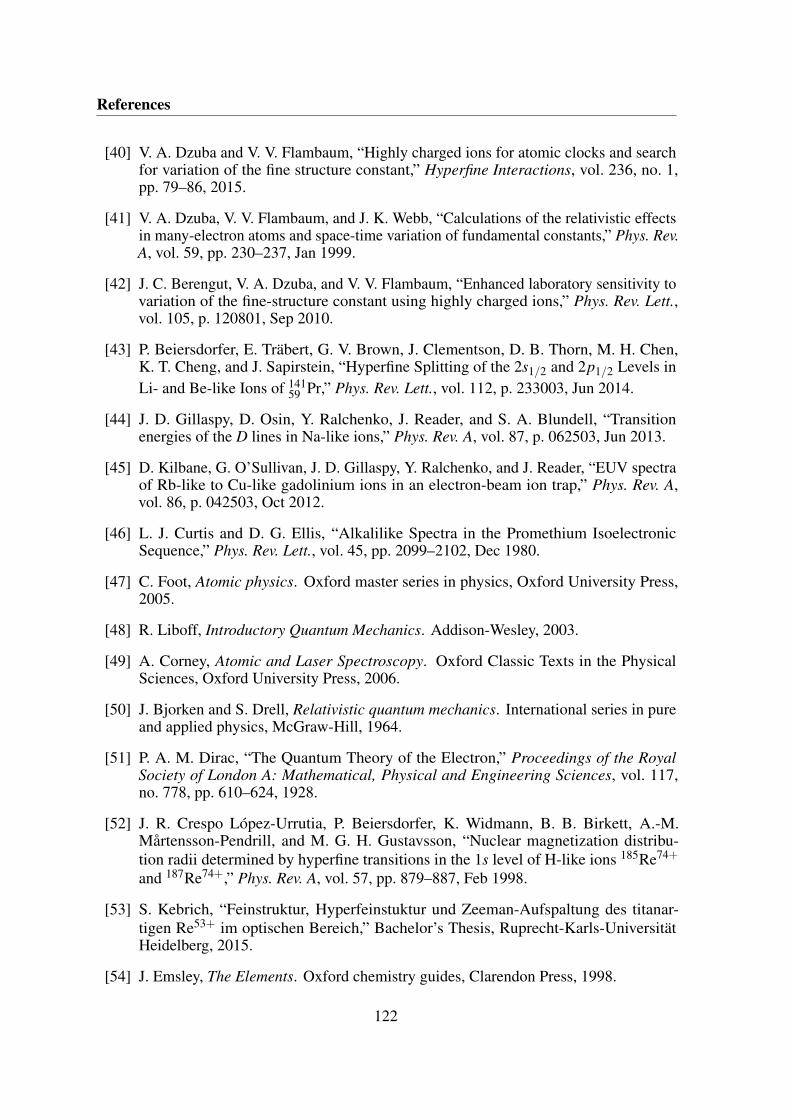
References
[40] V. A. Dzuba and V. V. Flambaum, “Highly charged ions for atomic clocks and searchfor variation of the fine structure constant,” Hyperfine Interactions, vol. 236, no. 1,pp. 79–86, 2015.
[41] V. A. Dzuba, V. V. Flambaum, and J. K. Webb, “Calculations of the relativistic effectsin many-electron atoms and space-time variation of fundamental constants,” Phys. Rev.A, vol. 59, pp. 230–237, Jan 1999.
[42] J. C. Berengut, V. A. Dzuba, and V. V. Flambaum, “Enhanced laboratory sensitivity tovariation of the fine-structure constant using highly charged ions,” Phys. Rev. Lett.,vol. 105, p. 120801, Sep 2010.
[43] P. Beiersdorfer, E. Träbert, G. V. Brown, J. Clementson, D. B. Thorn, M. H. Chen,K. T. Cheng, and J. Sapirstein, “Hyperfine Splitting of the 2s1/2 and 2p1/2 Levels inLi- and Be-like Ions of 141
59 Pr,” Phys. Rev. Lett., vol. 112, p. 233003, Jun 2014.
[44] J. D. Gillaspy, D. Osin, Y. Ralchenko, J. Reader, and S. A. Blundell, “Transitionenergies of the D lines in Na-like ions,” Phys. Rev. A, vol. 87, p. 062503, Jun 2013.
[45] D. Kilbane, G. O’Sullivan, J. D. Gillaspy, Y. Ralchenko, and J. Reader, “EUV spectraof Rb-like to Cu-like gadolinium ions in an electron-beam ion trap,” Phys. Rev. A,vol. 86, p. 042503, Oct 2012.
[46] L. J. Curtis and D. G. Ellis, “Alkalilike Spectra in the Promethium IsoelectronicSequence,” Phys. Rev. Lett., vol. 45, pp. 2099–2102, Dec 1980.
[47] C. Foot, Atomic physics. Oxford master series in physics, Oxford University Press,2005.
[48] R. Liboff, Introductory Quantum Mechanics. Addison-Wesley, 2003.
[49] A. Corney, Atomic and Laser Spectroscopy. Oxford Classic Texts in the PhysicalSciences, Oxford University Press, 2006.
[50] J. Bjorken and S. Drell, Relativistic quantum mechanics. International series in pureand applied physics, McGraw-Hill, 1964.
[51] P. A. M. Dirac, “The Quantum Theory of the Electron,” Proceedings of the RoyalSociety of London A: Mathematical, Physical and Engineering Sciences, vol. 117,no. 778, pp. 610–624, 1928.
[52] J. R. Crespo López-Urrutia, P. Beiersdorfer, K. Widmann, B. B. Birkett, A.-M.Mårtensson-Pendrill, and M. G. H. Gustavsson, “Nuclear magnetization distribu-tion radii determined by hyperfine transitions in the 1s level of H-like ions 185Re74+
and 187Re74+,” Phys. Rev. A, vol. 57, pp. 879–887, Feb 1998.
[53] S. Kebrich, “Feinstruktur, Hyperfeinstuktur und Zeeman-Aufspaltung des titanar-tigen Re53+ im optischen Bereich,” Bachelor’s Thesis, Ruprecht-Karls-UniversitätHeidelberg, 2015.
[54] J. Emsley, The Elements. Oxford chemistry guides, Clarendon Press, 1998.
122
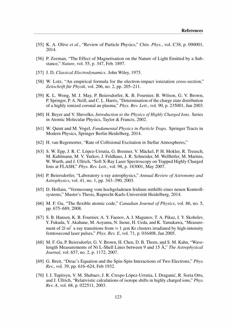
References
[55] K. A. Olive et al., “Review of Particle Physics,” Chin. Phys., vol. C38, p. 090001,2014.
[56] P. Zeeman, “The Effect of Magnetisation on the Nature of Light Emitted by a Sub-stance,” Nature, vol. 55, p. 347, Feb. 1897.
[57] J. D, Classical Electrodynamics. John Wiley, 1975.
[58] W. Lotz, “An empirical formula for the electron-impact ionization cross-section,”Zeitschrift für Physik, vol. 206, no. 2, pp. 205–211.
[59] K. L. Wong, M. J. May, P. Beiersdorfer, K. B. Fournier, B. Wilson, G. V. Brown,P. Springer, P. A. Neill, and C. L. Harris, “Determination of the charge state distributionof a highly ionized coronal au plasma,” Phys. Rev. Lett., vol. 90, p. 235001, Jun 2003.
[60] H. Beyer and V. Shevelko, Introduction to the Physics of Highly Charged Ions. Seriesin Atomic Molecular Physics, Taylor & Francis, 2002.
[61] W. Quint and M. Vogel, Fundamental Physics in Particle Traps. Springer Tracts inModern Physics, Springer Berlin Heidelberg, 2014.
[62] H. van Regemorter, “Rate of Collisional Excitation in Stellar Atmospheres,”
[63] S. W. Epp, J. R. C. López-Urrutia, G. Brenner, V. Mäckel, P. H. Mokler, R. Treusch,M. Kuhlmann, M. V. Yurkov, J. Feldhaus, J. R. Schneider, M. Wellhöfer, M. Martins,W. Wurth, and J. Ullrich, “Soft X-Ray Laser Spectroscopy on Trapped Highly ChargedIons at FLASH,” Phys. Rev. Lett., vol. 98, p. 183001, May 2007.
[64] P. Beiersdorfer, “Laboratory x-ray astrophysics,” Annual Review of Astronomy andAstrophysics, vol. 41, no. 1, pp. 343–390, 2003.
[65] D. Hollain, “Vermessung vom hochgeladenen Iridium mithilfe eines neuen Kontroll-systems,” Master’s Thesis, Ruprecht-Karls-Universität Heidelberg, 2014.
[66] M. F. Gu, “The flexible atomic code,” Canadian Journal of Physics, vol. 86, no. 5,pp. 675–689, 2008.
[67] S. B. Hansen, K. B. Fournier, A. Y. Faenov, A. I. Magunov, T. A. Pikuz, I. Y. Skobelev,Y. Fukuda, Y. Akahane, M. Aoyama, N. Inoue, H. Ueda, and K. Yamakawa, “Measure-ment of 2l-nl
′x-ray transitions from ≈ 1 µm Kr clusters irradiated by high-intensity
femtosecond laser pulses,” Phys. Rev. E, vol. 71, p. 016408, Jan 2005.
[68] M. F. Gu, P. Beiersdorfer, G. V. Brown, H. Chen, D. B. Thorn, and S. M. Kahn, “Wave-length Measurements of Ni L-Shell Lines between 9 and 15 Å,” The AstrophysicalJournal, vol. 657, no. 2, p. 1172, 2007.
[69] G. Breit, “Dirac’s Equation and the Spin-Spin Interactions of Two Electrons,” Phys.Rev., vol. 39, pp. 616–624, Feb 1932.
[70] I. I. Tupitsyn, V. M. Shabaev, J. R. Crespo López-Urrutia, I. Draganic, R. Soria Orts,and J. Ullrich, “Relativistic calculations of isotope shifts in highly charged ions,” Phys.Rev. A, vol. 68, p. 022511, 2003.
123
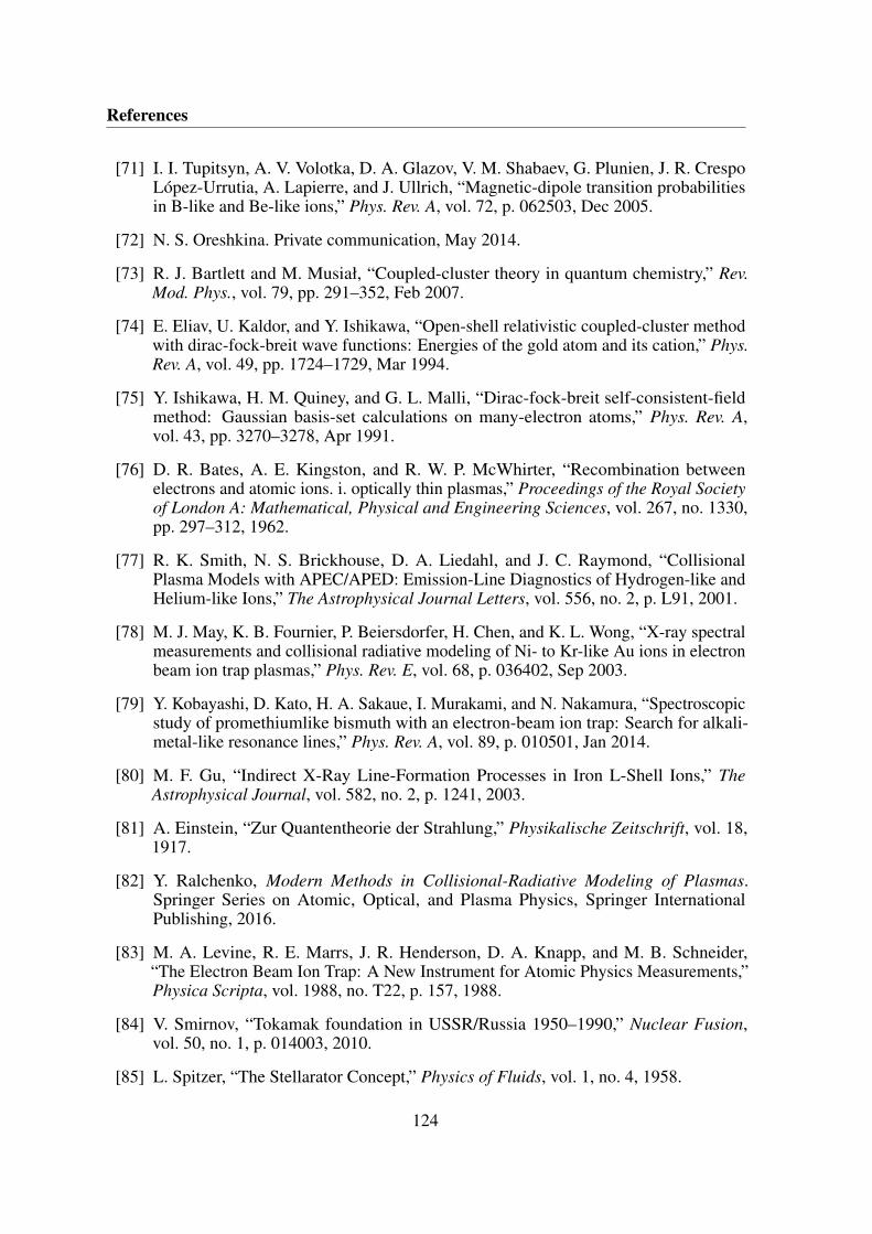
References
[71] I. I. Tupitsyn, A. V. Volotka, D. A. Glazov, V. M. Shabaev, G. Plunien, J. R. CrespoLópez-Urrutia, A. Lapierre, and J. Ullrich, “Magnetic-dipole transition probabilitiesin B-like and Be-like ions,” Phys. Rev. A, vol. 72, p. 062503, Dec 2005.
[72] N. S. Oreshkina. Private communication, May 2014.
[73] R. J. Bartlett and M. Musiał, “Coupled-cluster theory in quantum chemistry,” Rev.Mod. Phys., vol. 79, pp. 291–352, Feb 2007.
[74] E. Eliav, U. Kaldor, and Y. Ishikawa, “Open-shell relativistic coupled-cluster methodwith dirac-fock-breit wave functions: Energies of the gold atom and its cation,” Phys.Rev. A, vol. 49, pp. 1724–1729, Mar 1994.
[75] Y. Ishikawa, H. M. Quiney, and G. L. Malli, “Dirac-fock-breit self-consistent-fieldmethod: Gaussian basis-set calculations on many-electron atoms,” Phys. Rev. A,vol. 43, pp. 3270–3278, Apr 1991.
[76] D. R. Bates, A. E. Kingston, and R. W. P. McWhirter, “Recombination betweenelectrons and atomic ions. i. optically thin plasmas,” Proceedings of the Royal Societyof London A: Mathematical, Physical and Engineering Sciences, vol. 267, no. 1330,pp. 297–312, 1962.
[77] R. K. Smith, N. S. Brickhouse, D. A. Liedahl, and J. C. Raymond, “CollisionalPlasma Models with APEC/APED: Emission-Line Diagnostics of Hydrogen-like andHelium-like Ions,” The Astrophysical Journal Letters, vol. 556, no. 2, p. L91, 2001.
[78] M. J. May, K. B. Fournier, P. Beiersdorfer, H. Chen, and K. L. Wong, “X-ray spectralmeasurements and collisional radiative modeling of Ni- to Kr-like Au ions in electronbeam ion trap plasmas,” Phys. Rev. E, vol. 68, p. 036402, Sep 2003.
[79] Y. Kobayashi, D. Kato, H. A. Sakaue, I. Murakami, and N. Nakamura, “Spectroscopicstudy of promethiumlike bismuth with an electron-beam ion trap: Search for alkali-metal-like resonance lines,” Phys. Rev. A, vol. 89, p. 010501, Jan 2014.
[80] M. F. Gu, “Indirect X-Ray Line-Formation Processes in Iron L-Shell Ions,” TheAstrophysical Journal, vol. 582, no. 2, p. 1241, 2003.
[81] A. Einstein, “Zur Quantentheorie der Strahlung,” Physikalische Zeitschrift, vol. 18,1917.
[82] Y. Ralchenko, Modern Methods in Collisional-Radiative Modeling of Plasmas.Springer Series on Atomic, Optical, and Plasma Physics, Springer InternationalPublishing, 2016.
[83] M. A. Levine, R. E. Marrs, J. R. Henderson, D. A. Knapp, and M. B. Schneider,“The Electron Beam Ion Trap: A New Instrument for Atomic Physics Measurements,”Physica Scripta, vol. 1988, no. T22, p. 157, 1988.
[84] V. Smirnov, “Tokamak foundation in USSR/Russia 1950–1990,” Nuclear Fusion,vol. 50, no. 1, p. 014003, 2010.
[85] L. Spitzer, “The Stellarator Concept,” Physics of Fluids, vol. 1, no. 4, 1958.
124
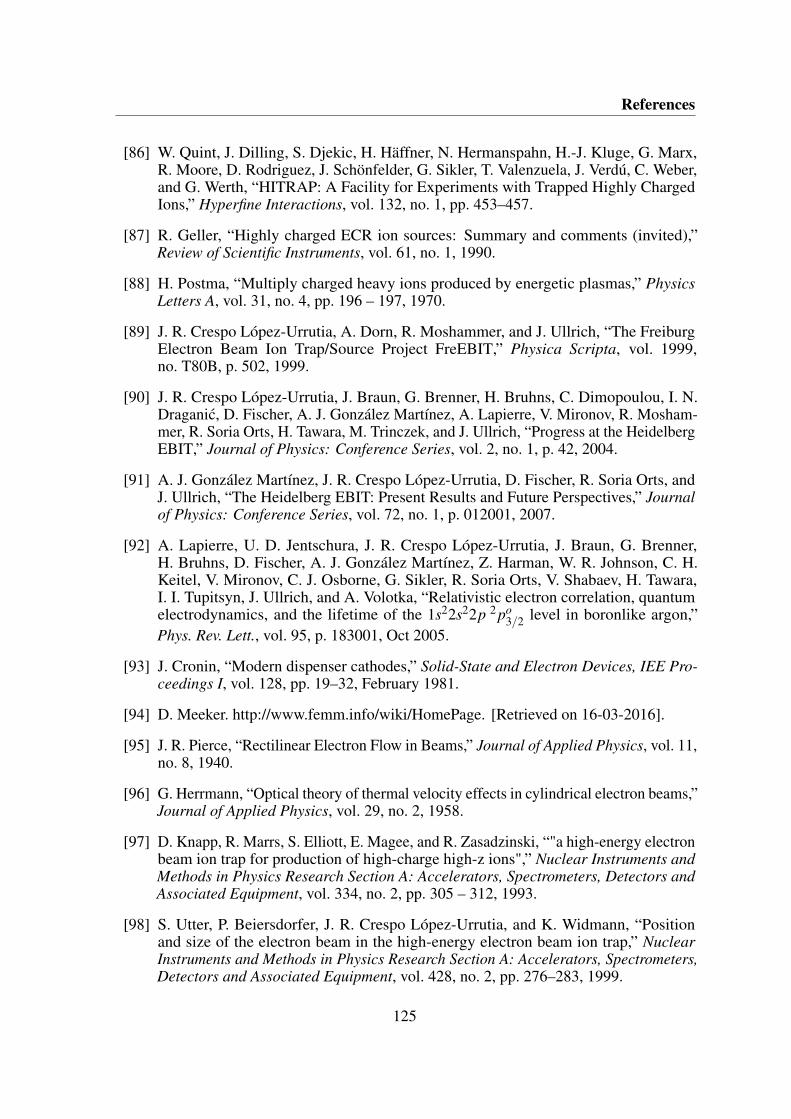
References
[86] W. Quint, J. Dilling, S. Djekic, H. Häffner, N. Hermanspahn, H.-J. Kluge, G. Marx,R. Moore, D. Rodriguez, J. Schönfelder, G. Sikler, T. Valenzuela, J. Verdú, C. Weber,and G. Werth, “HITRAP: A Facility for Experiments with Trapped Highly ChargedIons,” Hyperfine Interactions, vol. 132, no. 1, pp. 453–457.
[87] R. Geller, “Highly charged ECR ion sources: Summary and comments (invited),”Review of Scientific Instruments, vol. 61, no. 1, 1990.
[88] H. Postma, “Multiply charged heavy ions produced by energetic plasmas,” PhysicsLetters A, vol. 31, no. 4, pp. 196 – 197, 1970.
[89] J. R. Crespo López-Urrutia, A. Dorn, R. Moshammer, and J. Ullrich, “The FreiburgElectron Beam Ion Trap/Source Project FreEBIT,” Physica Scripta, vol. 1999,no. T80B, p. 502, 1999.
[90] J. R. Crespo López-Urrutia, J. Braun, G. Brenner, H. Bruhns, C. Dimopoulou, I. N.Draganic, D. Fischer, A. J. González Martínez, A. Lapierre, V. Mironov, R. Mosham-mer, R. Soria Orts, H. Tawara, M. Trinczek, and J. Ullrich, “Progress at the HeidelbergEBIT,” Journal of Physics: Conference Series, vol. 2, no. 1, p. 42, 2004.
[91] A. J. González Martínez, J. R. Crespo López-Urrutia, D. Fischer, R. Soria Orts, andJ. Ullrich, “The Heidelberg EBIT: Present Results and Future Perspectives,” Journalof Physics: Conference Series, vol. 72, no. 1, p. 012001, 2007.
[92] A. Lapierre, U. D. Jentschura, J. R. Crespo López-Urrutia, J. Braun, G. Brenner,H. Bruhns, D. Fischer, A. J. González Martínez, Z. Harman, W. R. Johnson, C. H.Keitel, V. Mironov, C. J. Osborne, G. Sikler, R. Soria Orts, V. Shabaev, H. Tawara,I. I. Tupitsyn, J. Ullrich, and A. Volotka, “Relativistic electron correlation, quantumelectrodynamics, and the lifetime of the 1s22s22p 2 po
3/2 level in boronlike argon,”Phys. Rev. Lett., vol. 95, p. 183001, Oct 2005.
[93] J. Cronin, “Modern dispenser cathodes,” Solid-State and Electron Devices, IEE Pro-ceedings I, vol. 128, pp. 19–32, February 1981.
[94] D. Meeker. http://www.femm.info/wiki/HomePage. [Retrieved on 16-03-2016].
[95] J. R. Pierce, “Rectilinear Electron Flow in Beams,” Journal of Applied Physics, vol. 11,no. 8, 1940.
[96] G. Herrmann, “Optical theory of thermal velocity effects in cylindrical electron beams,”Journal of Applied Physics, vol. 29, no. 2, 1958.
[97] D. Knapp, R. Marrs, S. Elliott, E. Magee, and R. Zasadzinski, “"a high-energy electronbeam ion trap for production of high-charge high-z ions",” Nuclear Instruments andMethods in Physics Research Section A: Accelerators, Spectrometers, Detectors andAssociated Equipment, vol. 334, no. 2, pp. 305 – 312, 1993.
[98] S. Utter, P. Beiersdorfer, J. R. Crespo López-Urrutia, and K. Widmann, “Positionand size of the electron beam in the high-energy electron beam ion trap,” NuclearInstruments and Methods in Physics Research Section A: Accelerators, Spectrometers,Detectors and Associated Equipment, vol. 428, no. 2, pp. 276–283, 1999.
125
References
[99] J. Gillaspy, Y. Aglitskiy, E. Bell, C. Brown, C. Chantler, R. Deslattes, U. Feldman,L. Hudson, J. Laming, E. Meyer, et al., “Overview of the electron beam ion trapprogram at nist,” Physica Scripta, vol. 1995, no. T59, p. 392, 1995.
[100] G. Y. Liang, J. R. Crespo López-Urrutia, T. M. Baumann, S. W. Epp, A. Gonchar,A. Lapierre, P. H. Mokler, M. C. Simon, H. Tawara, V. Mäckel, K. Yao, G. Zhao,Y. Zou, and J. Ullrich, “Experimental Investigations of Ion Charge Distributions,Effective Electron Densities, and Electron-Ion Cloud Overlap in Electron Beam IonTrap Plasma Using Extreme-Ultraviolet Spectroscopy,” The Astrophysical Journal,vol. 702, no. 2, p. 838, 2009.
[101] S. W. Epp, Röntgen-Laserspektroskopie hochgeladener Ionen in einer EBIT am Freie-Elektronen-Laser FLASH. PhD thesis, Ruprecht-Karls-Universität Heidelberg, 2005.
[102] R. E. Marrs, S. R. Elliott, and D. A. Knapp, “Production and trapping of hydrogenlikeand bare uranium ions in an electron beam ion trap,” Phys. Rev. Lett., vol. 72, pp. 4082–4085, Jun 1994.
[103] P. Beiersdorfer, V. Decaux, S. R. Elliott, K. Widmann, and K. Wong, “Temperatureof the ions produced and trapped in an electron-beam ion trap,” Review of ScientificInstruments, vol. 66, no. 1, 1995.
[104] V. Mäckel, R. Klawitter, G. Brenner, J. R. Crespo López-Urrutia, and J. Ullrich, “LaserSpectroscopy on Forbidden Transitions in Trapped Highly Charged Ar13+ Ions,” Phys.Rev. Lett., vol. 107, p. 143002, Sep 2011.
[105] C. Yamada, K. Nagata, N. Nakamura, S. Ohtani, S. Takahashi, T. Tobiyama, M. Tona,H. Watanabe, N. Yoshiyasu, M. Sakurai, A. P. Kavanagh, and F. J. Currell, “Injectionof metallic elements into an electron-beam ion trap using a Knudsen cell,” Review ofScientific Instruments, vol. 77, no. 6, 2006.
[106] G. E. Holland, C. N. Boyer, J. F. Seely, J. Tan, J. Pomeroy, and J. Gillaspy, “Low jittermetal vapor vacuum arc ion source for electron beam ion trap injections,” Review ofscientific instruments, vol. 76, no. 7, p. 073304, 2005.
[107] M. Trinczek, A. Werdich, V. Mironov, P. Guo, A. J. González Martínez, J. Braun,J. R. Crespo López-Urrutia, and J. Ullrich, “A laser ion source for an electron beamion trap,” Nuclear Instruments and Methods in Physics Research Section B: BeamInteractions with Materials and Atoms, vol. 251, no. 1, pp. 289–296, 2006.
[108] S. Elliott and R. Marrs, “A wire probe as an ion source for an electron beam ion trap,”Nuclear Instruments and Methods in Physics Research Section B: Beam Interactionswith Materials and Atoms, vol. 100, no. 4, pp. 529–535, 1995.
[109] Strem Chemicals, Inc., “Volatile Organometallics.” http://www.strem.com/catalog/family/Volatile+Organometallics+for+CVD+%26+ALD/. [Retrieved on 08-02-2016].
[110] K. Kromer, “Rekombinationsprozesse in hochgeladenem Bismut uns Praseodym,”Bachelor’s Thesis, Ruprecht-Karls-Universität Heidelberg, 2015.
[111] E. Hecht, Optics. Addison-Wesley, 2002.
126
References
[112] W. S. Boyle and G. E. Smith, “Charge coupled semiconductor devices,” Bell SystemTechnical Journal, vol. 49, no. 4, pp. 587–593, 1970.
[113] “Nobel prize in Physics 2009.” http://www.nobelprize.org/nobel_prizes/physics/laureates/2009/press.html. [Retrieved on 06-02-2016].
[114] R. Aymar, P. Barabaschi, and Y. Shimomura, “The ITER design,” Plasma Physics andControlled Fusion, vol. 44, no. 5, p. 519, 2002.
[115] T. Klinger, C. Baylard, C. Beidler, J. Boscary, H. Bosch, A. Dinklage, D. Hartmann,P. Helander, H. Maßberg, A. Peacock, T. Pedersen, T. Rummel, F. Schauer, L. We-gener, and R. Wolf, “Towards assembly completion and preparation of experimentalcampaigns of Wendelstein 7-X in the perspective of a path to a stellarator fusion powerplant,” Fusion Engineering and Design, vol. 88, no. 6–8, pp. 461 – 465, 2013. Pro-ceedings of the 27th Symposium On Fusion Technology (SOFT-27); Liège, Belgium,September 24-28, 2012.
[116] I. Hutchinson, Principles of Plasma Diagnostics. Cambridge University Press, 2002.
[117] R. Isler, R. Neidigh, and R. Cowan, “Tungsten radiation from tokamak-producedplasmas,” Physics Letters A, vol. 63, no. 3, pp. 295 – 297, 1977.
[118] C. Biedermann, R. Radtke, R. Seidel, and T. Pütterich, “Spectroscopy of highlycharged tungsten ions relevant to fusion plasmas,” Physica Scripta, vol. 2009, no. T134,p. 014026, 2009.
[119] E. Träbert and P. Heckmann, “Tentative identification of the 5s-5p transitions in PmI-like Au XIX,” Zeitschrift für Physik D Atoms, Molecules and Clusters, vol. 1, no. 4,pp. 381–383, 1986.
[120] K. B. Fournier, M. Finkenthal, S. Lippmann, C. P. Holmes, H. W. Moos, W. H.Goldstein, and A. L. Osterheld, “n = 5 to n = 5 soft-x-ray emission of uranium in ahigh-temperature low-density tokamak plasma,” Phys. Rev. A, vol. 50, pp. 3727–3733,Nov 1994.
[121] R. Hutton, Y. Zou, J. R. Almandos, C. Biedermann, R. Radtke, A. Greier, and R. Neu,“EBIT spectroscopy of Pm-like tungsten,” Nuclear Instruments and Methods in PhysicsResearch Section B: Beam Interactions with Materials and Atoms, vol. 205, no. 0,pp. 114 – 118, 2003. 11th International Conference on the Physics of Highly ChargedIons.
[122] M. J. Vilkas, Y. Ishikawa, and E. Träbert, “Electric-dipole 5s-5p transitions in prome-thiumlike ions,” Phys. Rev. A, vol. 77, p. 042510, Apr 2008.
[123] U. I. Safronova, A. S. Safronova, and P. Beiersdorfer, “Contribution of the 4 f -core-excited states in determination of atomic properties in the promethium isoelectronicsequence,” Phys. Rev. A, vol. 88, p. 032512, Sep 2013.
[124] U. I. Safronova, V. V. Flambaum, and M. S. Safronova, “Transitions between the4 f -core-excited states in Ir16+, Ir17+, and Ir18+ ions for clock applications,” vol. 92,p. 022501, Aug. 2015.
127
References
[125] T. M. Baumann, “Entwicklung eines Gitterspektrometers zur Untersuchung vakuu-multravioletter Strahlung von hochgeladenen Ionen,” Diplomarbeit, Ruprecht-Karls-Universität Heidelberg, 2008.
[126] J. A. R. Samson, Techniques of Vacuum Ultraviolet Spectroscopy. Lincoln, Nebraska:Pied Publications, 1967.
[127] T. Harada and T. Kita, “Mechanically ruled aberration-corrected concave gratings,”Appl. Opt., vol. 19, pp. 3987–3993, Dec 1980.
[128] T. Harada, K. Takahashi, H. Sakuma, and A. Osyczka, “Optimum design of a grazing-incidence flat-field spectrograph with a spherical varied-line-space grating,” Appl.Opt., vol. 38, pp. 2743–2748, May 1999.
[129] D. L. Windt, W. C. Cash, M. Scott, P. Arendt, B. Newnam, R. F. Fisher, and A. B.Swartzlander, “Optical constants for thin films of Ti, Zr, Nb, Mo, Ru, Rh, Pd, Ag, Hf,Ta, W, Re, Ir, Os, Pt, and Au from 24 Å to 1216 Å,” Appl. Opt., vol. 27, pp. 246–278,Jan 1988.
[130] A. Windberger, Identification of optical transitions in complex highly charged ions forapplications in metrology and tests of fundamental constants. PhD thesis, Ruprecht-Karls-Universität Heidelberg, 2015.
[131] R. Schupp, “Spektroskopische Untersuchung von Ir17+,” Bachelor’s Thesis, Ruprecht-Karls-Universität Heidelberg, 2008.
[132] O. Jitrik and C. F. Bunge, “Transition Probabilities for Hydrogen-Like Atoms,” J.Phys. Chem. Ref. Data, vol. 33, p. 1059, 2004.
[133] J. Scofield, “Ionisation Energies,” LLNL internal report, 1975.
[134] T. A. Carlson, C. N. Jr., N. Wasserman, and J. Mcdowell, “Calculated ionizationpotentials for multiply charged ions,” Atomic Data and Nuclear Data Tables, vol. 2,no. 0, pp. 63 – 99, 1970.
[135] LIGO Scientific Collaboration and Virgo Collaboration, “Observation of GravitationalWaves from a Binary Black Hole Merger,” Phys. Rev. Lett., vol. 116, p. 061102, Feb2016.
[136] R. Soria Orts, Isotopic effect in B-like and Be-like argon ions. PhD thesis, Ruprecht-Karls-Universität Heidelberg, 2005.
[137] R. Klawitter, “Resonant laser spectroscopy of a visible magnetic dipole transition inAr13+,” Diplomarbeit, Ruprecht-Karls-Universität Heidelberg, 2009.
[138] M. A. Blessenohl, “Optische Spektroskopie an hochgeladenen Bismut-Ionen und Kon-struktion eines hochauflösenden VUV-Gitterspektrometers,” Master’s thesis, Ruprecht-Karls-Universität Heidelberg, 2015.
[139] M. Czerny and A. F. Turner, “Über den Astigmatismus bei Spiegelspektrometern,”Zeitschrift für Physik, vol. 61, no. 11, p. 792–797.
128
References
[140] Princeton Instruments, “Spectroscopy Cameras.” http://www.princetoninstruments.com/products/speccam/pixis/dsheet.aspx. [Retrieved on 17-01-2016].
[141] Horiba Scientific, “Blazed Holographic Plane Gratings.” http://www.horiba.com/us/en/scientific/products/diffraction-gratings/for-industrial-applications/blazed-holographic-plane-gratings/grating-list/. [Retrieved on 24-01-2016].
[142] W. Pych, “A Fast Algorithm for Cosmic-Ray Removal from Single Images,” Pub-lications of the Astronomical Society of the Pacific, vol. 116, no. 816, pp. 148–153,2004.
[143] A. Z. Bonanos, K. Z. Stanek, R. P. Kudritzki, L. M. Macri, D. D. Sasselov, J. Kaluzny,P. B. Stetson, D. Bersier, F. Bresolin, T. Matheson, B. J. Mochejska, N. Przybilla, A. H.Szentgyorgyi, J. Tonry, and G. Torres, “The First DIRECT Distance Determinationto a Detached Eclipsing Binary in M33,” The Astrophysical Journal, vol. 652, no. 1,p. 313, 2006.
[144] W. Whaling, W. Anderson, M. Carle, J. Brault, and H. Zarem, “Argon ion linelist andlevel energies in the hollow-cathode discharge,” Journal of Quantitative Spectroscopyand Radiative Transfer, vol. 53, no. 1, pp. 1 – 22, 1995.
[145] I. G. Nave, S. Johansson, R. C. M. Learner, A. P. Thorne, and J. W. Brault, “A NewMultiplet Table for Fe,” 1994.
[146] B. Edlén, “The refractive index of air,” Metrologia, vol. 2, no. 2, p. 71, 1966.
[147] E. R. Peck and K. Reeder, “Dispersion of air,” J. Opt. Soc. Am., vol. 62, pp. 958–962,Aug 1972.
[148] N. S. Oreshkina. Private communication, November 2015.
[149] J. C. Berengut. Private communication, December 2014.
[150] L. Schmöger, O. O. Versolato, M. Schwarz, M. Kohnen, A. Windberger, B. Piest,S. Feuchtenbeiner, J. Pedregosa-Gutierrez, T. Leopold, P. Micke, A. K. Hansen, T. M.Baumann, M. Drewsen, J. Ullrich, P. O. Schmidt, and J. R. Crespo López-Urrutia,“Coulomb crystallization of highly charged ions,” Science, vol. 347, no. 6227, pp. 1233–1236, 2015.
[151] P. O. Schmidt, T. Rosenband, C. Langer, W. M. Itano, J. C. Bergquist, and D. J.Wineland, “Spectroscopy using quantum logic,” Science, vol. 309, no. 5735, pp. 749–752, 2005.
129

Appendix A
Predicted E1 line shapes
There are 24 possibly optical E1 transitions between the 4 f 135s1 and 4 f 125s2 configurations.Due to the 8.00 T magnetic field strength at the trap center, the line shapes of the transitionsis determined mainly by the Zeeman splitting of lines, refer to chapter 2. In this appendix,the predicted line shapes of the 24 E1 transitions are shown. The predictions were basedon the g j-factors as calculated by Berengut [34, 149]. The lines were assumed to have awidth of 25 ·10−5 eV, which corresponds to the resolving power of the employed opticalspectrometer at approximately 260 nm, 4.75 eV.
131
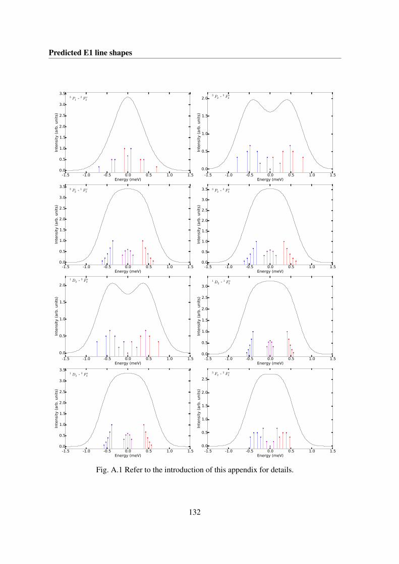
Predicted E1 line shapes
-1.5 -1.0 -0.5 0.0 0.5 1.0 1.5Energy (meV)
0.0
0.5
1.0
1.5
2.0
2.5
3.0
3.5
Inte
nsi
ty (
arb
. unit
s)
3 P1 - 3 F o2
-1.5 -1.0 -0.5 0.0 0.5 1.0 1.5Energy (meV)
0.0
0.5
1.0
1.5
2.0
Inte
nsi
ty (
arb
. unit
s)
3 P2 - 3 F o2
-1.5 -1.0 -0.5 0.0 0.5 1.0 1.5Energy (meV)
0.0
0.5
1.0
1.5
2.0
2.5
3.0
3.5
Inte
nsi
ty (
arb
. unit
s)
3 P2 - 1 F o3
-1.5 -1.0 -0.5 0.0 0.5 1.0 1.5Energy (meV)
0.0
0.5
1.0
1.5
2.0
2.5
3.0
3.5
Inte
nsi
ty (
arb
. unit
s)
3 P2 - 3 F o3
-1.5 -1.0 -0.5 0.0 0.5 1.0 1.5Energy (meV)
0.0
0.5
1.0
1.5
2.0
Inte
nsi
ty (
arb
. unit
s)
1 D2 - 3 F o2
-1.5 -1.0 -0.5 0.0 0.5 1.0 1.5Energy (meV)
0.0
0.5
1.0
1.5
2.0
2.5
3.0
Inte
nsi
ty (
arb
. unit
s)
1 D2 - 1 F o3
-1.5 -1.0 -0.5 0.0 0.5 1.0 1.5Energy (meV)
0.0
0.5
1.0
1.5
2.0
2.5
3.0
3.5
Inte
nsi
ty (
arb
. unit
s)
1 D2 - 3 F o3
-1.5 -1.0 -0.5 0.0 0.5 1.0 1.5Energy (meV)
0.0
0.5
1.0
1.5
2.0
2.5
Inte
nsi
ty (
arb
. unit
s)
3 F2 - 3 F o2
Fig. A.1 Refer to the introduction of this appendix for details.
132
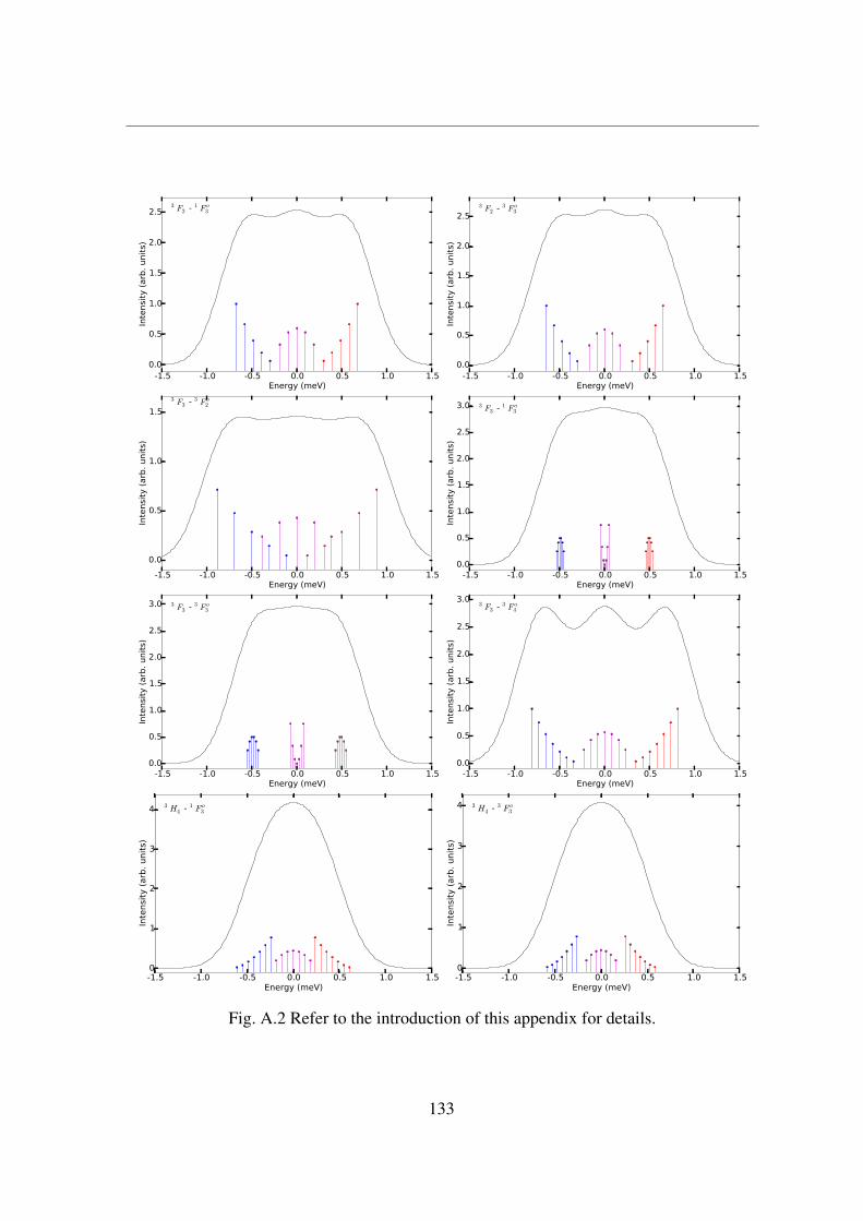
-1.5 -1.0 -0.5 0.0 0.5 1.0 1.5Energy (meV)
0.0
0.5
1.0
1.5
2.0
2.5
Inte
nsi
ty (
arb
. unit
s)
3 F2 - 1 F o3
-1.5 -1.0 -0.5 0.0 0.5 1.0 1.5Energy (meV)
0.0
0.5
1.0
1.5
2.0
2.5
Inte
nsi
ty (
arb
. unit
s)
3 F2 - 3 F o3
-1.5 -1.0 -0.5 0.0 0.5 1.0 1.5Energy (meV)
0.0
0.5
1.0
1.5
Inte
nsi
ty (
arb
. unit
s)
3 F3 - 3 F o2
-1.5 -1.0 -0.5 0.0 0.5 1.0 1.5Energy (meV)
0.0
0.5
1.0
1.5
2.0
2.5
3.0
Inte
nsi
ty (
arb
. unit
s)
3 F3 - 1 F o3
-1.5 -1.0 -0.5 0.0 0.5 1.0 1.5Energy (meV)
0.0
0.5
1.0
1.5
2.0
2.5
3.0
Inte
nsi
ty (
arb
. unit
s)
3 F3 - 3 F o3
-1.5 -1.0 -0.5 0.0 0.5 1.0 1.5Energy (meV)
0.0
0.5
1.0
1.5
2.0
2.5
3.0
Inte
nsi
ty (
arb
. unit
s)
3 F3 - 3 F o4
-1.5 -1.0 -0.5 0.0 0.5 1.0 1.5Energy (meV)
0
1
2
3
4
Inte
nsi
ty (
arb
. unit
s)
3 H4 - 1 F o3
-1.5 -1.0 -0.5 0.0 0.5 1.0 1.5Energy (meV)
0
1
2
3
4
Inte
nsi
ty (
arb
. unit
s)
3 H4 - 3 F o3
Fig. A.2 Refer to the introduction of this appendix for details.
133
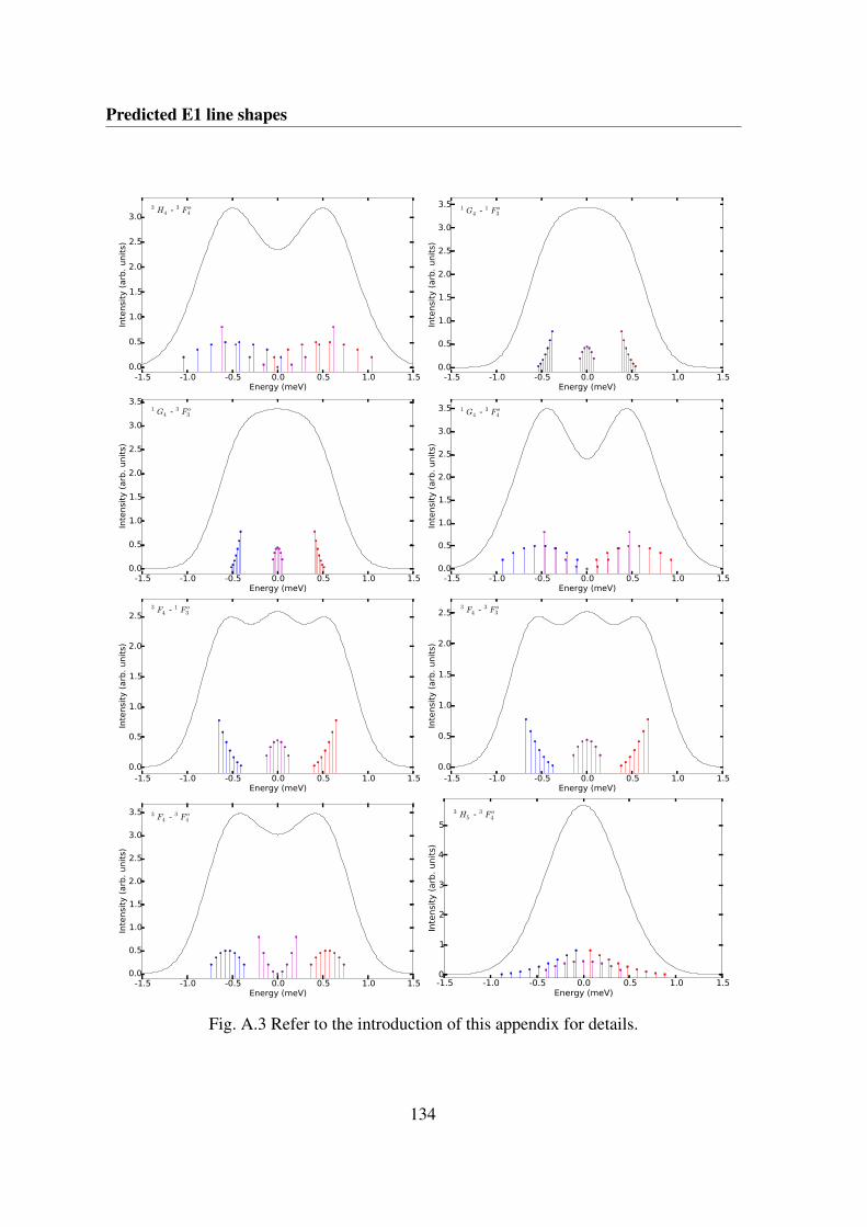
Predicted E1 line shapes
-1.5 -1.0 -0.5 0.0 0.5 1.0 1.5Energy (meV)
0.0
0.5
1.0
1.5
2.0
2.5
3.0
Inte
nsi
ty (
arb
. unit
s)
3 H4 - 3 F o4
-1.5 -1.0 -0.5 0.0 0.5 1.0 1.5Energy (meV)
0.0
0.5
1.0
1.5
2.0
2.5
3.0
3.5
Inte
nsi
ty (
arb
. unit
s)
1 G4 - 1 F o3
-1.5 -1.0 -0.5 0.0 0.5 1.0 1.5Energy (meV)
0.0
0.5
1.0
1.5
2.0
2.5
3.0
3.5
Inte
nsi
ty (
arb
. unit
s)
1 G4 - 3 F o3
-1.5 -1.0 -0.5 0.0 0.5 1.0 1.5Energy (meV)
0.0
0.5
1.0
1.5
2.0
2.5
3.0
3.5
Inte
nsi
ty (
arb
. unit
s)
1 G4 - 3 F o4
-1.5 -1.0 -0.5 0.0 0.5 1.0 1.5Energy (meV)
0.0
0.5
1.0
1.5
2.0
2.5
Inte
nsi
ty (
arb
. unit
s)
3 F4 - 1 F o3
-1.5 -1.0 -0.5 0.0 0.5 1.0 1.5Energy (meV)
0.0
0.5
1.0
1.5
2.0
2.5
Inte
nsi
ty (
arb
. unit
s)
3 F4 - 3 F o3
-1.5 -1.0 -0.5 0.0 0.5 1.0 1.5Energy (meV)
0.0
0.5
1.0
1.5
2.0
2.5
3.0
3.5
Inte
nsi
ty (
arb
. unit
s)
3 F4 - 3 F o4
-1.5 -1.0 -0.5 0.0 0.5 1.0 1.5Energy (meV)
0
1
2
3
4
5
Inte
nsi
ty (
arb
. unit
s)
3 H5 - 3 F o4
Fig. A.3 Refer to the introduction of this appendix for details.
134
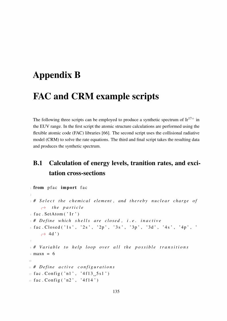
Appendix B
FAC and CRM example scripts
The following three scripts can be employed to produce a synthetic spectrum of Ir17+ inthe EUV range. In the first script the atomic structure calculations are performed using theflexible atomic code (FAC) libraries [66]. The second script uses the collisional radiativemodel (CRM) to solve the rate equations. The third and final script takes the resulting dataand produces the synthetic spectrum.
B.1 Calculation of energy levels, tranition rates, and exci-tation cross-sections
1 from p f a c import f a c2
3 # S e l e c t t h e c h e m i c a l e l emen t , and t h e r e b y n u c l e a r charge o f→ t h e p a r t i c l e
4 f a c . SetAtom ( ’ I r ’ )5 # D e f i n e which s h e l l s are c l o s e d , i . e . i n a c t i v e6 f a c . C losed ( ’ 1 s ’ , ’ 2 s ’ , ’ 2p ’ , ’ 3 s ’ , ’ 3p ’ , ’ 3d ’ , ’ 4 s ’ , ’ 4p ’ , ’
→ 4d ’ )7
8 # V a r i a b l e t o h e l p loop over a l l t h e p o s s i b l e t r a n s i t i o n s9 maxn = 6
10
11 # D e f i n e a c t i v e c o n f i g u r a t i o n s12 f a c . Conf ig ( ’ n1 ’ , ’ 4 f13 5 s1 ’ )13 f a c . Conf ig ( ’ n2 ’ , ’ 4 f14 ’ )
135

FAC and CRM example scripts
14 f a c . Conf ig ( ’ n3 ’ , ’ 4 f13 5p1 ’ )15 f a c . Conf ig ( ’ n4 ’ , ’ 4 f12 5 s2 ’ )16 f a c . Conf ig ( ’ n5 ’ , ’ 4 f12 5 s1 5p1 ’ )17 f a c . Conf ig ( ’ n6 ’ , ’ 4 f11 5 s2 5p1 ’ )18
19 # Determine t h e o p t i m a l r a d i a l p o t e n t i a l20 f a c . Conf igEnergy ( 0 )21 f a c . O p t i m i z e R a d i a l ( ’ n1 ’ )22 f a c . Conf igEnergy ( 1 )23
24 # To f i x t h e en er gy o f l e v e l s , uncomment t h e f o l l o w i n g l i n e→ and p r o v i d e a s u i t a b l e l i s t o f c o r r e c t i o n s
25 # f a c . C o r r e c t E n e r g y ( ’ c o r r e c t i o n s 2 b ’ , 0 )26
27 # C a l c u l a t e and save t h e f i n e −s t r u c t u r e l e v e l e n e r g i e s28 f a c . S t r u c t u r e ( ’ I r 1 7 p l u s _ b i n . en ’ , [ ’ n1 ’ , ’ n2 ’ , ’ n3 ’ , ’ n4 ’ , ’ n5 ’
→ , ’ n6 ’ ] )29 f a c . MemENTable ( ’ I r 1 7 p l u s _ b i n . en ’ )30 f a c . P r i n t T a b l e ( ’ I r 1 7 p l u s _ b i n . en ’ , ’ I r 1 7 p l u s . en ’ )31
32 # C a l c u l a t e and save t h e t r a n s i t i o n r a t e s33 f o r n in r a n g e ( 1 , maxn ) :34 f o r m in r a n g e ( n , maxn ) :35 # With t h e −1 t h e m u l t i p o l e t y p e i s s e l c t e d , E1 i n t h i s
→ case36 f a c . TRTable ( ’ I r 1 7 p l u s _ b i n . t r ’ , [ ’ n ’ + s t r ( n ) ] , [ ’ n ’ +
→ s t r (m) ] , −1)37 f a c . P r i n t T a b l e ( ’ I r 1 7 p l u s _ b i n . t r ’ , ’ I r 1 7 p l u s . t r ’ )38
39 # C a l c u l a t e and save t h e e l e c t r o n imp ac t c r o s s s e c t i o n s40 f o r n in r a n g e ( 1 , maxn ) :41 f o r m in r a n g e ( n , maxn ) :42 f a c . CETable ( ’ I r 1 7 p l u s _ b i n . ce ’ , [ ’ n ’ + s t r ( n ) ] , [ ’ n ’ + s t r
→ (m) ] )43 f a c . P r i n t T a b l e ( ’ I r 1 7 p l u s _ b i n . ce ’ , ’ I r 1 7 p l u s . ce ’ )
136

B.2 Collisional radiative model
B.2 Collisional radiative model
1 from p f a c import f a c2 from p f a c . crm import *3
4 # S e l e c t which i o n s are i n c l u d e d i n t h e CRM c a l c u l a t i o n5 AddIon ( 6 0 , 1 . 0 , ’ I r 1 7 p l u s _ b i n ’ )6
7 # 1: i f <0 o n l y t r a n s i t i o n w i t h i n 17+ are connec t ed , 2 : da ta→ f i l e n a m e s ( d e f a u l t e x t e n s i o n a u t o m a t i c a l l y added )
8 S e t B l o c k s (−1 , ’ I r 1 7 p l u s _ b i n ’ )9 P r i n t ( ’ b l o c k s s e t ’ )
10
11 # S e t p r o p e r t i e s o f t h e e l e c t r o n beam12 # 1: g a u s s i a n e l e c t r o n en er g y d i s t r i b u t i o n , 2 : e l e c t r o n beam
→ e ne rg y i n eV , 3 : e ne rg y sp re ad i n eV , 4 and 5: Emin→ and Emax
13 S e t E l e D i s t ( 1 , 440 , 5 , 435 , 445)14
15 # Photon r a t e s . 0 means : t a k e o n l y p o n t a n e o u s decay i n t o→ ac ou n t
16 SetTRRates ( 0 )17
18 # C o l l i s i o n a l t r a n s i t i o n r a t e s . I f 1 : i n c l u d e bo th→ c o l l i s i o n a l e x c i t a t i o n and de− e x c i t a t i o n . I f 0 : o n l y→ e x c i t a t i o n
19 SetCERates ( 1 )20
21 # S e t t h e e l e c t r o n d e n s i t y i n u n i t s o f 1 e10 cm^−322 S e t E l e D e n s i t y ( 1 0 0 )23
24 # S o l v e t h e c o u p l e d d i f f e r e n t i a l e q u a t i o n s25 I n i t B l o c k s ( )26 S e t I t e r a t i o n (1 e−6, 0 . 5 , 2048)27
28 # Determine t h e l e v e l p o p u l a t i o n s and save t h e da ta
137
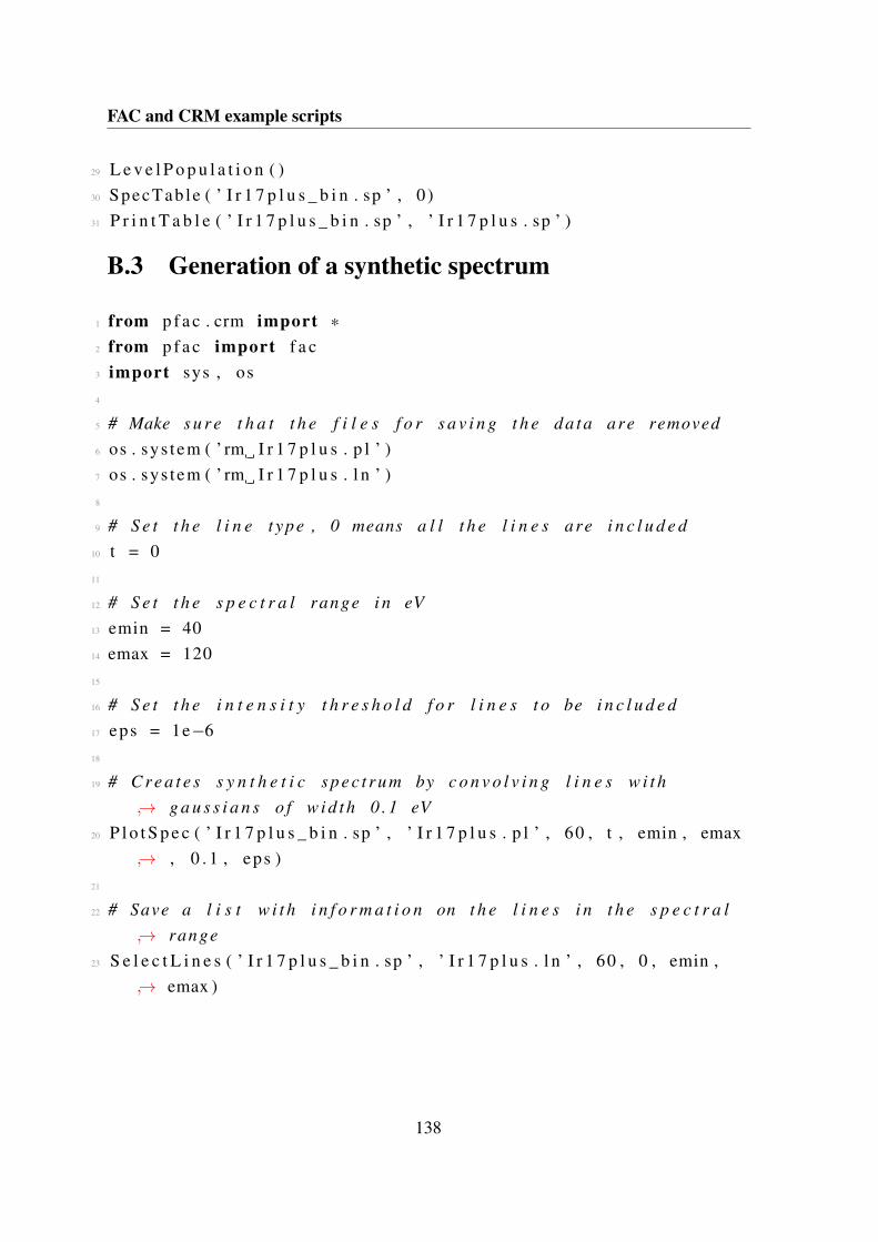
FAC and CRM example scripts
29 L e v e l P o p u l a t i o n ( )30 SpecTab le ( ’ I r 1 7 p l u s _ b i n . sp ’ , 0 )31 P r i n t T a b l e ( ’ I r 1 7 p l u s _ b i n . sp ’ , ’ I r 1 7 p l u s . sp ’ )
B.3 Generation of a synthetic spectrum
1 from p f a c . crm import *2 from p f a c import f a c3 import sys , os4
5 # Make s u r e t h a t t h e f i l e s f o r s a v i n g t h e da ta are removed6 os . sys tem ( ’ rm I r 1 7 p l u s . p l ’ )7 os . sys tem ( ’ rm I r 1 7 p l u s . l n ’ )8
9 # S e t t h e l i n e t ype , 0 means a l l t h e l i n e s are i n c l u d e d10 t = 011
12 # S e t t h e s p e c t r a l range i n eV13 emin = 4014 emax = 12015
16 # S e t t h e i n t e n s i t y t h r e s h o l d f o r l i n e s t o be i n c l u d e d17 eps = 1e−618
19 # C r e a t e s s y n t h e t i c s p e c t r u m by c o n v o l v i n g l i n e s w i t h→ g a u s s i a n s o f w i d t h 0 . 1 eV
20 P l o t S p e c ( ’ I r 1 7 p l u s _ b i n . sp ’ , ’ I r 1 7 p l u s . p l ’ , 60 , t , emin , emax→ , 0 . 1 , eps )
21
22 # Save a l i s t w i t h i n f o r m a t i o n on t h e l i n e s i n t h e s p e c t r a l→ range
23 S e l e c t L i n e s ( ’ I r 1 7 p l u s _ b i n . sp ’ , ’ I r 1 7 p l u s . l n ’ , 60 , 0 , emin ,→ emax )
138

Appendix C
EUV lines of Nd-like and Pr-like Re, Os,Ir, and Pt
139
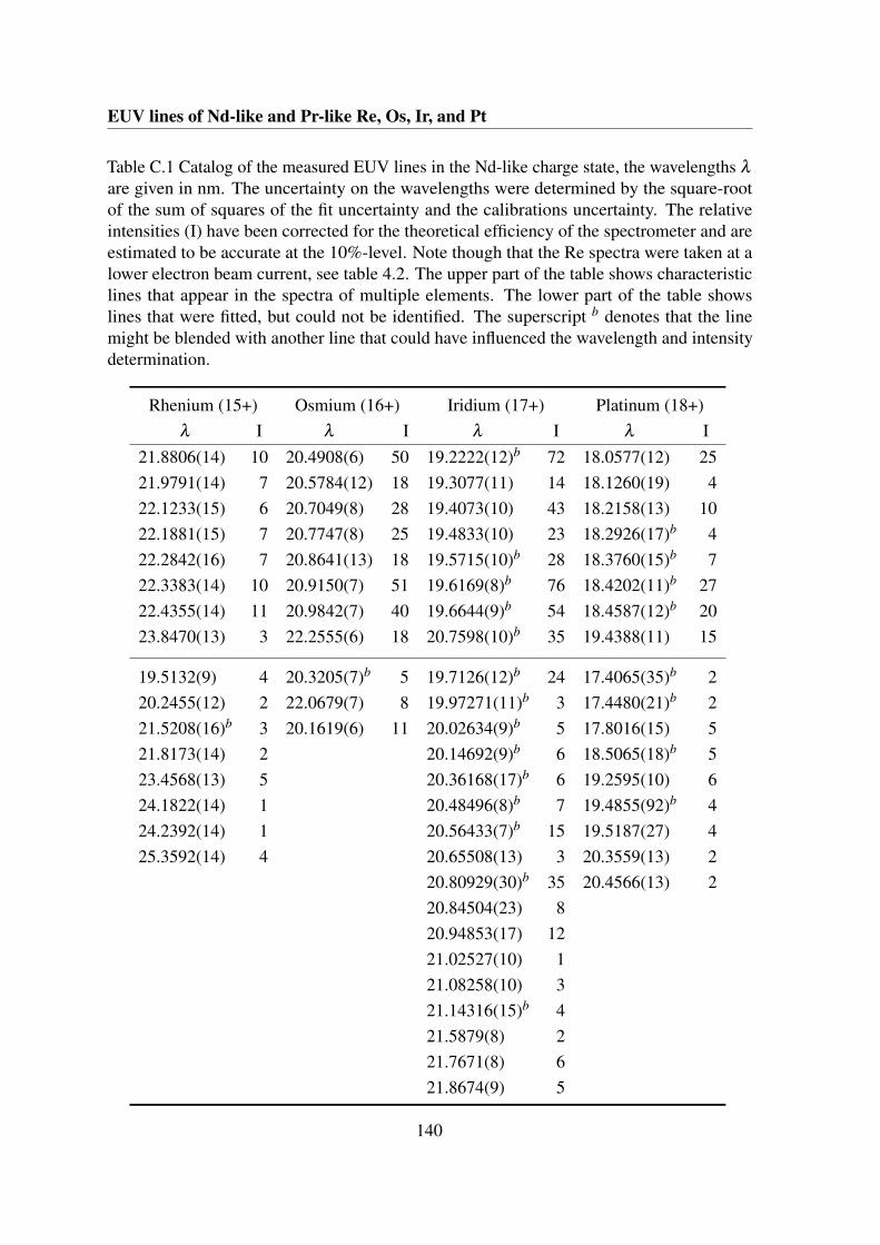
EUV lines of Nd-like and Pr-like Re, Os, Ir, and Pt
Table C.1 Catalog of the measured EUV lines in the Nd-like charge state, the wavelengths λ
are given in nm. The uncertainty on the wavelengths were determined by the square-rootof the sum of squares of the fit uncertainty and the calibrations uncertainty. The relativeintensities (I) have been corrected for the theoretical efficiency of the spectrometer and areestimated to be accurate at the 10%-level. Note though that the Re spectra were taken at alower electron beam current, see table 4.2. The upper part of the table shows characteristiclines that appear in the spectra of multiple elements. The lower part of the table showslines that were fitted, but could not be identified. The superscript b denotes that the linemight be blended with another line that could have influenced the wavelength and intensitydetermination.
Rhenium (15+) Osmium (16+) Iridium (17+) Platinum (18+)λ I λ I λ I λ I
21.8806(14) 10 20.4908(6) 50 19.2222(12)b 72 18.0577(12) 2521.9791(14) 7 20.5784(12) 18 19.3077(11) 14 18.1260(19) 422.1233(15) 6 20.7049(8) 28 19.4073(10) 43 18.2158(13) 1022.1881(15) 7 20.7747(8) 25 19.4833(10) 23 18.2926(17)b 422.2842(16) 7 20.8641(13) 18 19.5715(10)b 28 18.3760(15)b 722.3383(14) 10 20.9150(7) 51 19.6169(8)b 76 18.4202(11)b 2722.4355(14) 11 20.9842(7) 40 19.6644(9)b 54 18.4587(12)b 2023.8470(13) 3 22.2555(6) 18 20.7598(10)b 35 19.4388(11) 15
19.5132(9) 4 20.3205(7)b 5 19.7126(12)b 24 17.4065(35)b 220.2455(12) 2 22.0679(7) 8 19.97271(11)b 3 17.4480(21)b 221.5208(16)b 3 20.1619(6) 11 20.02634(9)b 5 17.8016(15) 521.8173(14) 2 20.14692(9)b 6 18.5065(18)b 523.4568(13) 5 20.36168(17)b 6 19.2595(10) 624.1822(14) 1 20.48496(8)b 7 19.4855(92)b 424.2392(14) 1 20.56433(7)b 15 19.5187(27) 425.3592(14) 4 20.65508(13) 3 20.3559(13) 2
20.80929(30)b 35 20.4566(13) 220.84504(23) 820.94853(17) 1221.02527(10) 121.08258(10) 321.14316(15)b 421.5879(8) 221.7671(8) 621.8674(9) 5
140
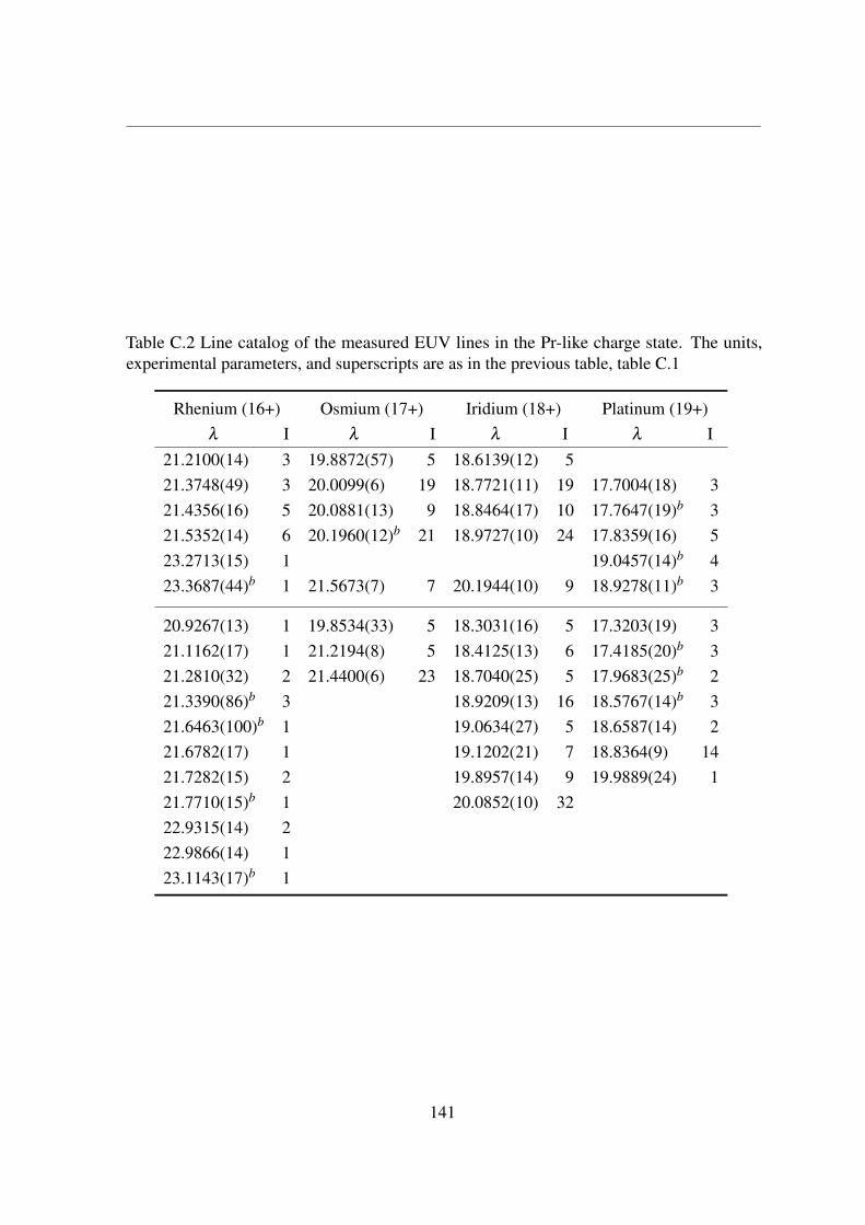
Table C.2 Line catalog of the measured EUV lines in the Pr-like charge state. The units,experimental parameters, and superscripts are as in the previous table, table C.1
Rhenium (16+) Osmium (17+) Iridium (18+) Platinum (19+)λ I λ I λ I λ I
21.2100(14) 3 19.8872(57) 5 18.6139(12) 521.3748(49) 3 20.0099(6) 19 18.7721(11) 19 17.7004(18) 321.4356(16) 5 20.0881(13) 9 18.8464(17) 10 17.7647(19)b 321.5352(14) 6 20.1960(12)b 21 18.9727(10) 24 17.8359(16) 523.2713(15) 1 19.0457(14)b 423.3687(44)b 1 21.5673(7) 7 20.1944(10) 9 18.9278(11)b 3
20.9267(13) 1 19.8534(33) 5 18.3031(16) 5 17.3203(19) 321.1162(17) 1 21.2194(8) 5 18.4125(13) 6 17.4185(20)b 321.2810(32) 2 21.4400(6) 23 18.7040(25) 5 17.9683(25)b 221.3390(86)b 3 18.9209(13) 16 18.5767(14)b 321.6463(100)b 1 19.0634(27) 5 18.6587(14) 221.6782(17) 1 19.1202(21) 7 18.8364(9) 1421.7282(15) 2 19.8957(14) 9 19.9889(24) 121.7710(15)b 1 20.0852(10) 3222.9315(14) 222.9866(14) 123.1143(17)b 1
141


Erklärung:
Ich versichere, dass ich diese Arbeit selbstständig verfasst und keine anderen als die angegebe-nen Quellen und Hilfsmittel benutzt habe.
Heidelberg, den .................... ..................................Hendrik Bekker
Related Documents