Opportunity-based block replacement

46 European Journal of Operational Research 53 (1991)46-63 North-Holland

Theory and Methodology

Opportunity-based block replacement Rommer t Dekker * and Eric Smeitink * *

Koninklijke / Shell-Laboratorium, Amsterdam P.O. Box 3003, 1003 AA Amsterdam, Netherlands

Received January 1989; revised November 1989

Abstract: In this paper we consider a block replacement model in which a component can be replaced preventively at maintenance opportunities only. Maintenance opportunities occur randomly and are modelled through a renewal process. In the first, theoretical part of the paper we derive an optimality equation and show that the optimal opportunity block replacement policy can be described as a so-called one-opportunity-look-ahead policy. In the second, computational part we present an exact optimisation algorithm in case of K2-distributed times between opportunities. This algorithm can also be used as an approximative method in case of other times between opportunity distributions. Together with another approximative method, based on the stationary forward recurrence time distribution, its performance is checked with simulation.

Keywords: Maintenance, optimisation, stochastic processes, probability, phase type distributions

1. Introduction

Preventive maintenance is widely accepted within industry as an effective means to reduce the number of failures. Preferably, it is planned at those moments in time when units are not required for production. In the process industry this may cause problems as most units are used continuously and downtime costs are high. Sometimes, however, there may be shortlasting interruptions of production for a variety of reasons, e.g. breakdowns of essential units. During these interruptions some other units are not required and these can then be maintained preventively without costs for downtime being incurred, in which case we speak of maintenance opportunities. Unfortunately, in most cases these opportunities cannot be predicted in advance.

Because of their random occurrence, traditional planning fails to make effective use of these mainte- nance opportunities. Within the Koninkli jke/Shell-Laboratorium, Amsterdam a decision support system has been developed for opportunity maintenance, which is now being field-tested. At the occurrence of an opportunity, the system aids the maintenance engineer in selecting, and assigning priorities to, preventive maintenance activities so as to minimise long-term total average costs.

In this paper we deal with one of the underlying models, viz. the opportunity block replacement model. In this model, a component is replaced upon failure and can only be replaced preventively at an opportunity. The occurrence of opportunities is described by a renewal process. The preventive replace-

* Present address: Shell International Petroleum Maatschappij B.V., P.O. Box 162, 2501 AN The Hague, Netherlands ** Present address: Faculty of Economy and Econometrics, Free University, P.O. Box 7161, 1007 MC Amsterdam, Netherlands.

0377-2217/91/$03.50 © 1991 - Elsevier Science Publishers B.V. (North-Holland)

R. Dekker, E. Smeitink / Opportunity-based block replacement 47

ment policies considered prescribe that a component be replaced preventively at the first opportunity after a critical time since the last preventive replacement.

This model was applied for units consisting of many components which were replaced individually upon failure and for which opportunities were created by causes outside the unit (e.g. breakdown of other essential units in a series configuration with the unit). Failures of components provided no maintenance opportunity for other components in the unit as the failure cause had to be removed as soon as possible and there was no time for preventive maintenance on that unit.

The simple age and block replacement model has been widely studied (see e.g. Barlow and Proschan [3]). Models for opportunity (or opportunistic) replacement, however, are scarce. Early work is reported in the review of Pierskalla and Voelker [14] and the book of Jorgenson et al. [11]. More recent work is discussed in the review of Sherif and Smith [17] and in the studies by Sherif [18] and B~ickert and Rippin [2].

Although there are few papers, they present several types of opportunity models. A number of papers consider multiple components and assume that failures of some components create opportunities for preventive maintenance of others. Our model can be regarded as a special case of these models. Discrete-time Markov decision chains are often used to analyse these models, but the computational effort is only bearable in case of few discrete lifetimes and few components. Besides, optimal policies tend to have complex structures and application of these models to our problem yields inferior results compared to our direct approach. A continuous time approach is given in [4]. The solution of the differential equations involved in his approach is only possible in case of special lifetime distributions, such as Erlang distributions.

A model in which opportunities were generated independently of the components to be maintained was first introduced by Jorgenson et al. [11]. For age replacement and exponential times between opportunities they provided formulas for operating characteristics, such as the average costs. For this case Woodman [22] and Duncan and Scholnick [8] provide some numerical results. Sethi [16] considered generally discrete-distributed lifetimes with Markov decision chains and showed that there exists an optimal policy of the control-limit type (a control-limit policy prescribes that a component be replaced at an opportunity if its age has passed a certain critical value). However, he does not show how to determine such a policy. Age replacement at deterministic times between opportunities was incorporated in a model analysed by Berg and Epstein [6].

In our model the opportunity generating process is separated from the component lifetime process, and in case of block replacement this allows a more general and elegant analysis, because the preventive maintenance action only depends on the opportunity process and not on realisations of the lifetimes. It further allows a far better insight into the effect of characteristics of the opportunity process on the optimal policy and the minimum average costs. Although in principle age replacement is a better policy than block replacement, it does not allow such a nice analysis as for block replacement, because at any failure one has to keep track of the residual time to the next opportunity, which has a simple form only in case of exponentially distributed times between opportunities. The opportunity age replacement model is therefore far more difficult to analyse in case of non-exponentially distributed times between opportuni- ties. The exponential case will be dealt with in a subsequent paper (see Dekker and Dijkstra [7]). A further disadvantage of age replacement is that extensions to replacement of multiple components are very difficult, which is not the case for block replacement.

The only paper that has dealt with opportunity block replacement so far is from Liang [12], (he uses the term piggyback policies) whose analysis is only a first step as he provides formulas for operating characteristics (such as average costs) in case of zero control limits only.

In this paper we give theoretical as well as computational results for general continuously distributed lifetimes and times between opportunities. In the theoretical part we focus on establishing an optimality equation without restrictive assumptions and provide an interpretation. In the computational part we present for a special class of opportunity distributions (including the exponential) an exact optimisation algorithm and show how this method can be used as an approximative method for general distributions. Simulation studies are carried out to check the approximations.

48 R. Dekker, E. Smeitink / Opportunity-based block replacement

2. The Opportunity Block Replacement Problem (OBRP)

Consider a component which may be replaced preventively at an opportunity only against costs Cp (> 0). Failure of the component with successive replacement induces costs cf (cf > Cp). Replacements are considered to occur instantaneously. The lifetimes of the components used for replacement are indepen- dent and identically distributed; they are represented by the continuous r.v. X with (finite) expectation ~t and variance o 2. Let F(t), f(t), M(t) and m(t) denote the corresponding cumulative distribution function (c.d.f.), probability density function (p.d.f.), renewal function and renewal density function, respectively. Opportunities occur according to a renewal process, independently of the lifetime process. Let the continuous r.v. Y denote the time between opportunities (abbreviated to TBO). We assume that Y has finite first and second moments and by G(t), g(t), N(t), and n(t) we denote its corresponding c.d.f., p.d.f., renewal function and renewal density function, respectively. We will further assume that both F(t) and G(t) are twice continuously differentiable and that F(0) = G(0) = 0. As a result both M(t) and N(t) are twice continuously differentiable. For the renewal density m(t) and the renewal function M(t) we have the following asymptotic expressions (see Ross [15] and Tijms [21]). Similar expressions hold for n(t) and N(t).

and

1 lim re(t)= - (1)

l - ' * ~ /.L

lira ( M ( t ) - ~ ) ° 2 1 ,~ ~ = 2/z 2 2" (2)

We will first state some results from the literature (see e.g. Barlow and Proschan [3] and Berg [5]) on the block replacement problem (abbreviated to BRP). That problem can be considered to be an extreme case of the OBRP by setting the time between opportunities equal to zero (and keeping the cost figures the same). We will refer to this case as the planned case, as it is possible to plan the preventive replacements in advance. In the planned case the process is renewed after each preventive replacement. According to the renewal reward theorem the long-term average costs ~p(t) associated with a replacement interval of length t are given by

Cp + cfM(t) % ( t ) = t , t > o. (3)

Differentiating (3) with respect to t and rewriting q~p(t) = 0 yields the equation which the optimal block replacement interval tp has to satisfy, i.e.

tin(t) - M(t) = Cp/Cf. (4)

Furthermore, the minimum expected long-term average cost ~p* (if a solution of (4) exists) equals

~ ; = ~ p ( t ; ) = c f m ( t ; ) . (5)

The marginal cost Bp(t) of a preventive replacement at time t (or more precisely, t units of time after the preceding preventive replacement) is defined as the difference, per unit time, between a preventive replacement now and the expected cost associated with waiting an additional infinitesimally short time A. More precisely,

( o f ( r e ( t ) a + o ( Z ) ) + c . ) -- cp Bp(t) = a-01im A = cfm(t), (6)

since re(t) A is the expected number of failures in (t, t + A), given only (failures are not recorded) that a

R. Dekker, E. Smeitink / Opportunity-based block replacement 49

* should satisfy is therefore new component was introduced at time 0. The equation which tp

~p(t) = ,~p(t), (v)

which is equivalent to (5) and which we will refer to as the optimality equation for the planned case. The following theorem from [5] gives sufficient conditions under which a unique, finite solution t~

exists.

Theorem 1. If m(t) is a continuously increasing function of t then equation (5) has a unique finite solution t~, pro~,ided that

- - < ½ 1 - . (8 ) C f

In the following we will generalize the aforementioned theory and especially the marginal cost approach from [5] to the opportunity block replacement model. Under an opportunity block replacement policy with control limit t a component is replaced preventively at the first opportunity which is at least t time units after the last preventive replacement. It is easily observed that preventive replacements at opportunities are renewals of the total process (both opportunity and lifetime). The process between two successive renewals will be called a cycle. The length of a cycle and the expected number of failures during a cycle depend on the control limit t and the (distribution of the) time between t and the first opportunity after t. Let Z, be the random variable denoting the time between t and the first opportunity after t (the forward recurrence time) and let q'(t, • ) be its c.d.f. Let us first recall some results from renewal theory which can be found in e.g. [15], pp. 44-45. With respect to the distribution of the forward recurrence time it can be shown that

and

P ( Z , < ~ z ) = G ( t + z ) - f o t { 1 - G ( t + z - u ) } d N ( u ) , t>~O, z>~O, (9 )

EZ~=EY{1 + N ( t ) ) =t, t>~O. (10)

Furthermore, there exists a limiting forward recurrence time distribution for which the following equation holds:

P(Z ~z)= lim P(Z,~z)= ~-~V ff'(1-G(u)} du, z>_0. (11) t ~ O 0 ]Lai J 0

Now we are able to give an expression for the long-term average costs Or ( t ) for an opportunity block replacement policy with control limit t

( J0 ) O r ( t ) = Cp+Cf M(t+z)dB(Z,<~z) / ( t+EZ , ) . (12)

Notice that the finiteness of EZ, and the fact that M(t) permits majoration by a linear function (which follows from (2)) guarantee the finiteness of the integral in (12) and that

lim M ( t + z ) ( 1 - P ( Z , < ~ z ) } = 0 forevery t>~0. (13) 2 ~ O O

Hence, we can rewrite the integral in (12) with partial integration in the following way

£ M(t + z) de(Z, ~ z) = M(t) + m(t + z){1 - P(Z, ~ z)} dz. (14)

In order to optimise 4~r ( t) we require the following technical lemma which mainly concerns the change of

50 R. Dekker, E. Smeitink / Opportunity-based block replacement

order of differentiation and integration of the integral on the right-hand side of (14). Its proof is given in Appendix 1.

Lemma 2. Let A(t) ~ f~m( t + z){1 - P(Z t <~ z)} dz. Then A(t) is differentiable in t and

ffd A ' ( t ) = -~[m(t+z){1-P(Z,~z))] dz

fo ~ m <~ =-m(t)+EYn(t) (t+z) dP(Z z). (15)

Notice that the derivative of A(t) depends only upon Z and not on Z,. Let

fo •y(t)==-cf m ( t + z ) dP(Z<~z) , (16)

and consider the following equation:

n y ( t ) - ~ r ( t ) = 0. (17)

We are now in a position to formulate the main theorem of opportunity block replacement and show that (17) is an optimality equation. The theorem is a direct generalisation of Theorem 1.

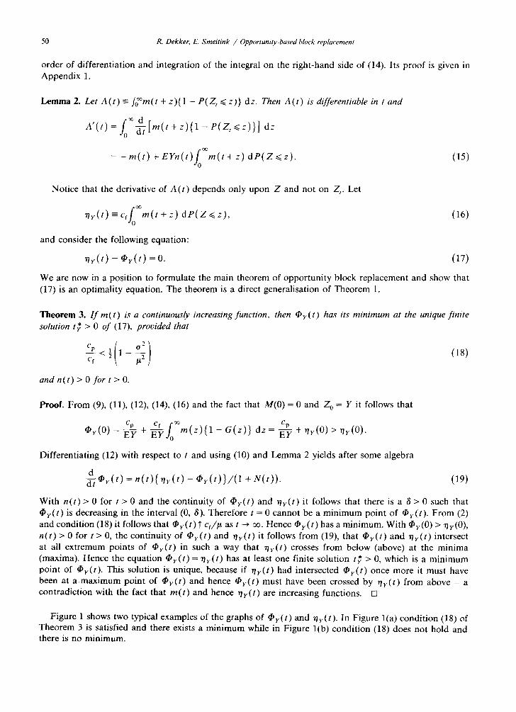
Theorem 3. I f re(t) is a continuously increasing function, then ~y( t) has its minimum at the unique finite solution t~, > 0 of (17), provided that

- - < ½ 1 - (18) Cf

and n(t) > 0 for t > O.

Proof. From (9), (11), (12), (14), (16) and the fact that M(0) = 0 and Z 0 -- Y it follows that

Cp Cf foe / ", Cp • r ( 0 ) = ~ - ~ + E - - Y J 0 m t z / { 1 - G ( z ) } d z = ~ - ~ + ~ y ( 0 ) > ~ y ( 0 ) .

Differentiating (12) with respect to t and using (10) and Lemma 2 yields after some algebra

d ~ r ( t ) --- n ( t ) { nr( t ) - ~ y ( t ) } / ( 1 + N(t) ) . (19)

With n(t) > 0 for t > 0 and the continuity of ~r( t ) and ~r(t) it follows that there is a 6 > 0 such that ~ r ( t ) is decreasing in the interval (0, 6). Therefore t = 0 cannot be a minimum point of ~v ( t ) . From (2) and condition (18) it follows that ~y( t ) "r cf/l~ as t ~ ~ . Hence ~ r ( t ) has a minimum. With ~ r ( 0 ) > ~r (0), n(t) > 0 for t > 0, the continuity of q~r(t) and ~r(t) it follows from (19), that ~ r ( t ) and ~y(t) intersect at all extremum points of Cby(t) in such a way that ~v ( t ) crosses from below (above) at the minima (maxima). Hence the equation ~ r ( t ) = ~ly(t) has at least one finite solution t~ > 0, which is a minimum point of ~ r ( t ) . This solution is unique, because if ~v(t) had intersected ~y( t ) once more it must have been at a m a x i m u m point of ~ r ( t ) and hence q~r(t) must have been crossed by ~ r ( t ) from above - a contradiction with the fact that re(t) and hence ~ly(t) are increasing functions. []

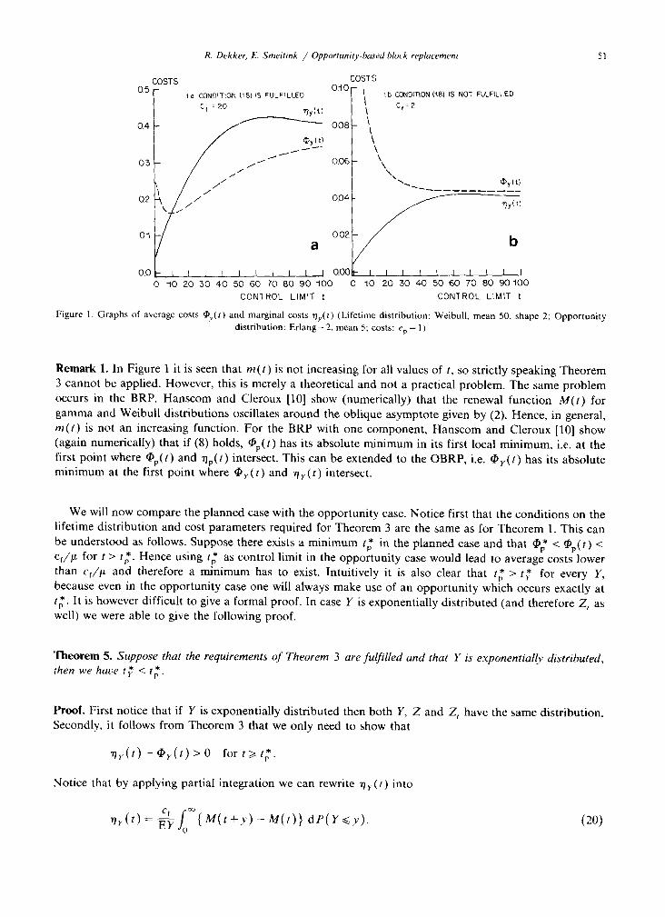
Figure 1 shows two typical examples of the graphs of ~r( t ) and ~r(t). In Figure l(a) condition (18) of Theorem 3 is satisfied and there exists a minimum while in Figure l(b) condition (18) does not hold and there is no minimum.

R. Dekker E. Smeitink / Opportunity-based block replacement 51

COSTS 0.5

0.4

03

Q2

O~

t e CONOITION riB) iS FULFILLED Cf : 20 r/y(t)

//// ///.~_.

/ /

a

COSTS

OJO ~ Of:2

008 \ \ \

OO6 \ \ \

0 0 4 -

002 /

lb CONDITION (~8) IS NOT FULFILLED

~y (t)

~y(t)

b

I I I t l 0.0 l" [ I I [ l I ~ [ 1 ~ 0 .00 I t 1 1 I 0 -t0 20 30 4 0 50 60 70 80 9 0 "100 0 "lO 2-0 30 40 .50 60 70 80 90 1 0 0

CONTROL LIMIT t CONTROL LIMIT t

Figure 1. G r a p h s o f average cos t s ~ v ( t ) a n d m a r g i n a l cos t s f ly ( t ) ( L i f e t i m e d i s tr ibut ion: W e i b u l l , m e a n 50, s h a p e 2; O p p o r t u n i t y d i s t r ibut ion: E r l a n g - 2 , mean 5: costs: Cp = 1)

Remark 1. In Figure 1 it is seen that re(t) is not increasing for all values of t, so strictly speaking Theorem 3 cannot be applied. However, this is merely a theoretical and not a practical problem. The same problem occurs in the BRP. Hanscom and Cleroux [10] show (numerically) that the renewal function M(t ) for gamma and Weibuil distributions oscillates around the oblique asymptote given by (2). Hence, in general, re(t) is not an increasing function. For the BRP with one component, Hanscom and Cleroux [10] show (again numerically) that if (8) holds, <bp(t) has its absolute minimum in its first local minimum, i.e. at the first point where ~p(t) and rip(t) intersect. This can be extended to the OBRP, i.e. ~ y ( t ) has its absolute minimum at the first point where q~y(t) and rir(t) intersect.

We will now compare the planned case with the opportunity case. Notice first that the conditions on the lifetime distribution and cost parameters required for Theorem 3 are the same as for Theorem 1. This can be understood as follows. Suppose there exists a minimum t~ in the planned case and that ~p* < ~p(t) < cf/ / , for t > tp. Hence using tp as control limit in the opportunity case would lead to average costs lower than cJ/~ and therefore a minimum has to exist. Intuitively it is also clear that t~ > t~ for every Y, because even in the opportunity case one will always make use of an opportunity which occurs exactly at

* It is however difficult to give a formal proof. In case Y is exponentially distributed (and therefore Z, as l p .

well) we were able to give the following proof.

Theorem 5. Suppose that the requirements of Theorem 3 are fulfilled and that Y is exponentially distributed, then we have t~ < t p.

Proof. First notice that if Y is exponentially distributed then both Y, Z and Z, have the same distribution. Secondly, it follows from Theorem 3 that we only need to show that

riy(t)-~r(t)>O for t>~ t~.

Notice that by applying partial integration we can rewrite riv(t) into

n~(t)= ErS0Cf [~tM(t+y)-~t(t))t dP(Y~y). (20)

52 R. Dekker, E. Smeitink / Opportunity-based block replacement

Combining the foregoing yields

~lr(t) - ~v ( t ) = fo ~ cr ( M ( t +Y)EY- M ( t ) } Cp + crM( t + y )

t + E Y d P ( Y ~ y )

o, c f tM( t+y) cfM(t) = fo EY(t + EY) EY

Cp t + E Y dP(Y<~y).

* we have For t >/t o

c o + cfM(t +y) c o + q M ( t ) > for all y > 0. t + y t

Hence,

c f tM( t+y)>ycp + ( t + y ) c f M ( t ), t>~tp, y > 0 .

Inserting this into (21) yields after some algebra

- E Y cfM(t)] dP(Y<~y) O, ,y ( t ) - f 0 Ey 7; [c0 + =

which completes the proof. []

(21)

3. T h e o n e - o p p o r t u n i t y - l o o k - a h e a d s t r a t e g y

In Section 2 we obtained the equation of optimality, (17), for the OBRP by minimising the expected cost per unit time, ~y(t), associated with the control limit policy t. We will now show that (17) has an intrinsic meaning, comparable with the marginal cost notion ~/p(t) in the BRP as introduced in [5].

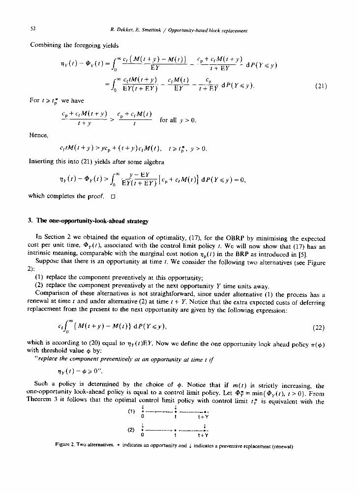
Suppose that there is an opportunity at time t. We consider the following two alternatives (see Figure 2):

(1) replace the component preventively at this opportunity; (2) replace the component preventively at the next opportunity Y time units away. Comparison of these alternatives is not straightforward, since under alternative (1) the process has a

renewal at time t and under alternative (2) at time t + Y. Notice that the extra expected costs of deferring replacement from the present to the next opportunity are given by the following expression:

Ctfo~( M(t + y) - M( t ) ) d P ( Y <~y), (22)

which is according to (20) equal to *lv(t)EY. Now we define the one opportunity look ahead policy rr(q,) with threshold value q~ by:

"replace the component preventively at an opportunity at time t if

ny(t) -+>~o".

Such a policy is determined by the choice of q~. Notice that if re(t) is strictly increasing, the one-opportunity look-ahead policy is equal to a control limit policy. Let ~ , -~ min{ ~y(t), t > 0}. From Theorem 3 it follows that the optimal control limit policy with control limit t~. is equivalent with the

(1) • . . . . . . . . . . . . . • . . . . . . . . . . ,_ 0 t t + Y

(2) * .............. • . . . . . . . . . . . , - o t t + Y

Figure 2. Two alternatives. * indicates an opportunity and ~, indicates a preventive replacement (renewal)

R. Dekker, E. Smeitink / Opportunity-based block replacement 53

one-opportunity-look-ahead policy with threshold value q)~. In order words, at each opportunity the extra expected costs of deferring preventive replacement to the next opportunity, ~r( t )EY , are compared with the minimum average costs, ~ , , times EY. Let ~r(~r(~)) denote the average costs under the one-oppor- tunity-look-ahead policy 7r(~,) with threshold value q). We have the following theorem

Theorem 6. I f re(t) is strictly increasing in t and condition (18) holds, then for every ~ for which q~, <~ ~p < ct/t~ we have

• ,,(~({~)) ~( ~p, (23)

with equality only if ~ = cb ~,.

Proof. For t~' < t < ~ we have ~lv(t)> ~ r ( t ) and l i m , ~ O v ( t ) = ct/l~. Hence for any q, satisfying ~ <~ q~ < cf/l~ there exists a t I > t~' with ~r( t l ) = q~ if 4} :g q~, and t 1 = t~' if ~ = cb~. Hence ~r(q~) is equivalent to a control limit policy with control limit t] and ~.(~r(40) = ~br(t2) from which the assertion directly follows. []

Remark 2. In most cases the curve of ~v( t ) crosses the curve of ~ v ( t ) in its minimum at a rather large angle (e.g. 70 ° in figure l(a)). Accordingly a small error made in calculating ~b~ is weakened by using the one-opportunity-look-ahead-policy, as also Theorem 6 states. If in the example of Figure l(a), we would use 4} = 0.215 ~ ~v(30) (instead of ~ v ( t ~ ) ~ 4)r(10 ) ~ 0.161) then the resulting one-opportunity-look- ahead policy is equivalent to a control limit policy with control limit t ' = 15 (~y(15)~0 .212) and associated expected long term average costs ~v(15) = 0.168 ~ ~v(t~? ).

4. Computational aspects

In this section we present methods to determine the optimal control limit t~ for the OBRP and the associated expected long-term average cost, i.e. the optimal threshold value ~ = qbr(t~). Our aim is to develop fast and robust methods which can be used in a decision support system. In doing so we want to use insensitivities and approximations provided that no substantial errors are introduced. The optimal policy t~, can be obtained by solving the equation of optimality (17) (see also Theorem 3). This can be done in a numerically very efficient and simple way with a bisection or regula falsi method. It only requires an interval [t a, tb] that contains the unique solution t~ and the functions epv(t ) and v/r(t). From (12) and (16) it is seen that calculation of ~v( t ) and cbv(t ) requires

(1) an algorithm to approximate the renewal function M(t) , since in general no analytical expression for M(t ) exists;

(2) the distribution function P(Z~ <~ z) of the time between t and the first opportunity after t (forward recurrence time) and its expectation;

(3) numerical integration of improper integrals. We will not go into detail about the numerical integration. Truncating the improper integrals should be

done with care because the tail of the distribution of the forward recurrence time may have a large contribution in case of large coefficients of variation. Good algorithms exist to treat improper integrals as the one in (12).We used an algorithm based on Gauss-Laguerre expansion which performed very well (see e.g. [20]).

4.1. A new method to approximate the renewal function

For most distributions used in reliability (e.g. the Weibull, gamma, and truncated normal distributions) no analytical expression for the renewal function M(t ) exists. There are several methods to approximate the renewal function, e.g. power series expansion and discretisation (see e.g. [9]). Calculating and

54 R. Dekker, E. Smeitink / Opportunity-based block replacement

optimising @v(t) involves repeated calculation of M(t) . Using the OBRP in a decision support system therefore requires a very fast and robust approximation for the renewal function. We developed a simple but effective method in which the original distribution is approximated by a phase-type distribution with the same first and second moment, for which the renewal function can be easily computed. We used the Ek-~,k distribution to approximate lifetime distributions with squared coefficient of variation c ~ ( - o 2/122 )

2 ~< ½ and the K 2 distribution (also called Coxian-2 distribution) in case c x > ½ (see [21, pp. 397-400]). The approximation Ml(t ) has the following form

oo Ml( t ) = r ( t ) + ~ i ( n ' ( t ) , t >1 O, (24a)

n=2

or equivalently,

Ml( t ) = A I ( t ) + [ r ( t ) - i f ( t ) ] , t>~0, (24b)

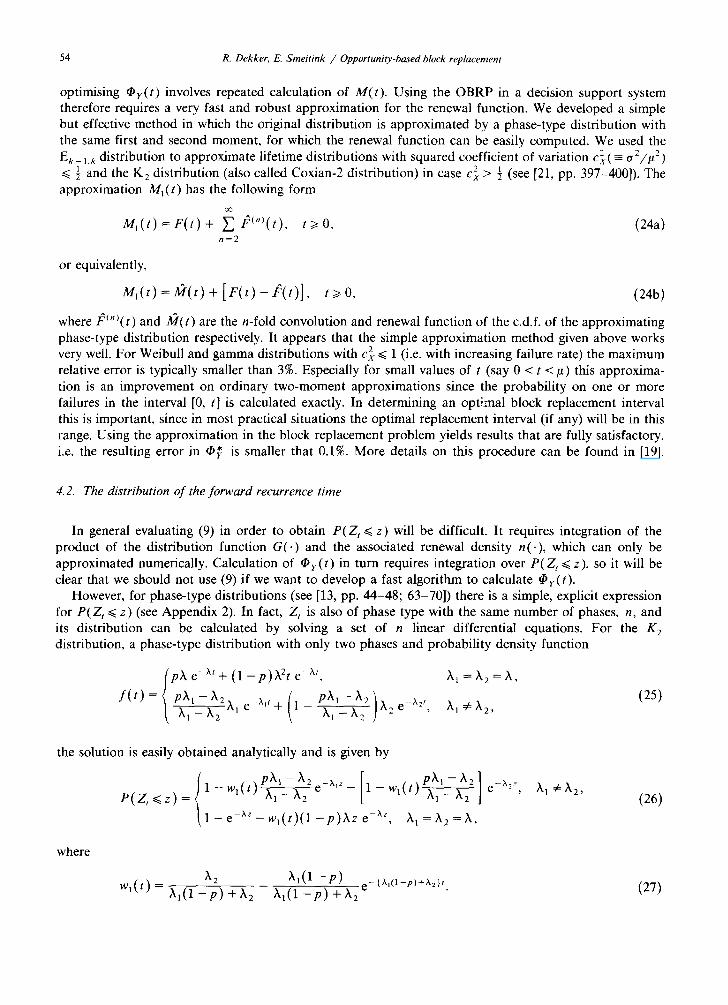
where fftn)(t) and 1Q(t) are the n-fold convolution and renewal function of the c.d.f, of the approximating phase-type distribution respectively. It appears that the simple approximation method given above works very well. For Weibull and gamma distributions with c 2 ~< 1 (i.e. with increasing failure rate) the maximum relative error is typically smaller than 3%. Especially for small values of t (say 0 < t < #) this approxima- tion is an improvement on ordinary two-moment approximations since the probability on one or more failures in the interval [0, t] is calculated exactly. In determining an optimal block replacement interval this is important, since in most practical situations the optimal replacement interval (if any) will be in this range. Using the approximation in the block replacement problem yields results that are fully satisfactory, i.e. the resulting error in ~ , is smaller that 0.1%. More details on this procedure can be found in [19].

4.2. The distribution of the forward recurrence time

In general evaluating (9) in order to obtain P ( Z t ~ z) will be difficult. It requires integration of the product of the distribution function G(.) and the associated renewal density n(.), which can only be approximated numerically. Calculation of ~ r ( t ) in turn requires integration over P ( Z t ~< z), so it will be clear that we should not use (9) if we want to develop a fast algorithm to calculate ~r( t ) .

However, for phase-type distributions (see [13, pp. 44-48; 63-70]) there is a simple, explicit expression for P ( Z t <~ z) (see Appendix 2). In fact, Z t is also of phase type with the same number of phases, n, and its distribution can be calculated by solving a set of n linear differential equations. For the K 2 distribution, a phase-type distribution with only two phases and probability density function

f ( t ) =

p)t e -A' + (1 - p ) X 2 t e -At,

PXl -)t2 ( P ~ ' l - - ) k 2 ) ~ll --~22 X, e -AIr --{- 1 ~ll-_~-X- ~ )k 2 e -A2t,

Xl =X2 = k ,

X1 4: X2, (25)

the solution is easily obtained analytically and is given by

P ( Z t < ~ z ) = 1 - w ~ ( t ) ~-a-X-~2 e -A~z- 1 - W l ( t ) ~-T-~-~2 e x2z,

1 - e - x ~ - w , ( t ) ( 1 - p ) x z e -Az, X,=X 2=X,

X 1 4: X2, (26)

where

~'2 Wl(t ) = }kl( 1 - - p ) q-~k 2

_ Xl(1 - - p ) e - {A,(1-p)+X2}t. X~(1 - p ) + X2 (27)

R. Dekker, E. Srneitink / Opportunity-based hlock replacement 55

PROB. DENSITY

" t0 SQUARED COEF OF VAR 0 5

0,8 ~ STAT

04

02 - - t -O 0 ~ ~

O0 ~ ~ l i ,

0 -1 2 3 4 TIME

PROB DENSITY 2 0 SOU~EO COEF OF VAR 2 0

- - t : O 0

-1.5 b~-----t : 0 2

~ t : 0 5 -10

0 5 ~

O0 r i __ , 0 I 2

I I 3 4

TIME

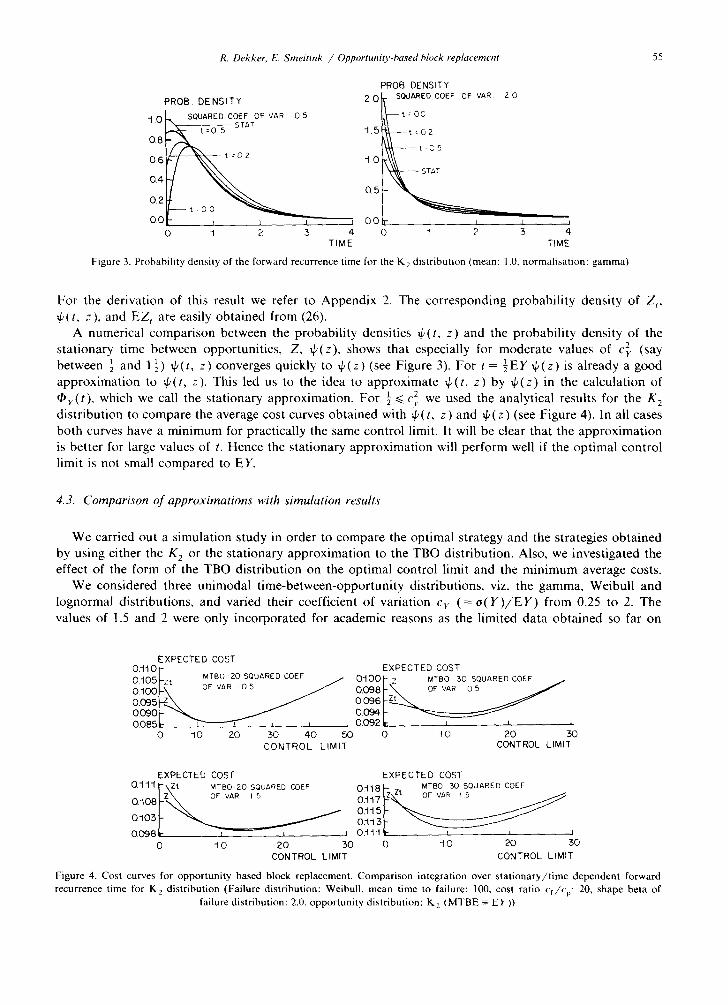
Figure 3. Probability density of the forward recurrence time for the K 2 distribution (mean: 1.0, normalisation: gamma)

For the derivation of this result we refer to Appendix 2. The corresponding probability density of Z,, +(t , .z), and EZ, are easily obtained from (26).

A numerical comparison between the probability densities +(t , z) and the probability density of the stationary time between opportunities, Z, + (z ) , shows that especially for moderate values of cey (say between ½ and 1 ~) q~(t, z) converges quickly to q~(z) (see Figure 3). For t = ½EY ~ ( z ) is already a good approximation to ~(t , z). This led us to the idea to approximate ~b(t, z) by q~(z) in the calculation of ~br(t ), which we call the stationary approximation. For ~ ~< c~ we used the analytical results for the K 2 distribution to compare the average cost curves obtained with + (t, z) and ~ (z) (see Figure 4). In all cases both curves have a minimum for practically the same control limit. It will be clear that the approximation is better for large values of t. Hence the stationary approximation will perform well if the optimal control limit is not small compared to EY.

4.3. Comparison of approximations with simulation results

We carried out a simulation study in order to compare the optimal strategy and the strategies obtained by using either the K 2 or the stationary approximation to the TBO distribution. Also, we investigated the effect of the form of the TBO distribution on the optimal control limit and the minimum average costs.

We considered three unimodal time-between-opportunity distributions, viz. the gamma, Weibuil and lognormal distributions, and varied their coefficient of variation Cy ( = o ( Y ) / E Y ) from 0.25 to 2. The values of 1.5 and 2 were only incorporated for academic reasons as the limited data obtained so far on

EXPECTED COST 0-110p EXPECTED COST ~4~=1 MT80 20 SQUARED COEF ~ 0-100~- Z MTBO 30 SQUARED COEF . / . . . . . zF ~ v 0-100 OF AR os 0 0 9 8 F \ OF VAR 05 /

0o901- ~ / o.o~F - ' ~ 0.085~ I -~- - " - -T I L L 0.0921r I L

0 -10 20 30 40 50 0 I 0 20 30 CONTROL LIMIT CONTROL LIMIT

EXPECTED COST EXPECTED COST 0.'1"f-1 ~-\ZL MTBO 20 SQUARED COEF 0 t 1 8 I . L 7 , MTBO 50 SQUARED COEF o.-1oBLZ\, , oF vAR ,5 O F . _ _ VAR

0.098E : - - L I O.-1"H It L h I 0 "10 20 30 0 -10 20 30

CONTROL LIMIT CONTROL LIMIT

Figure 4. Cost curves for opportunity based block replacement. Comparison integration over stat ionary/t ime dependent forward recurrence time for K 2 distribution (Failure distribution: Weibull, mean time to failure: 100, cost ratio cf/%: 20, shape beta of

failure distribution: 2.0, opportunity distribution: K 2 (MTBE --- EY ))

56 R. Dekker, E. Smeitink / Opportunity-based block replacement

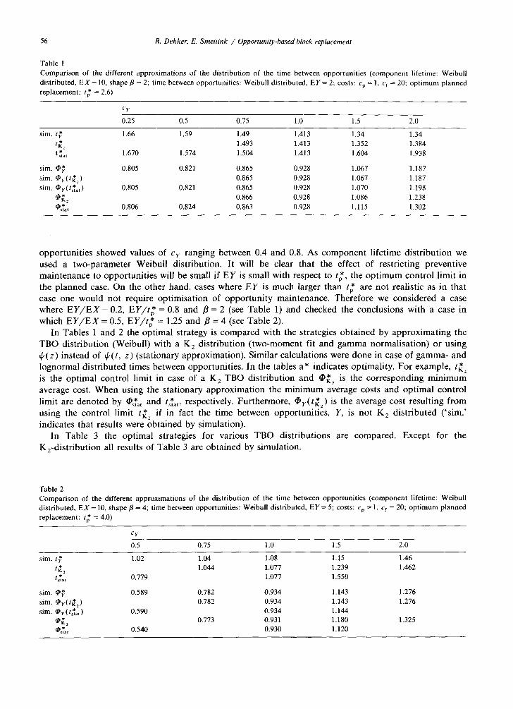
Table 1 Comparison of the different approximations of the distribution of the time between opportunities (component lifetime: Weibull distributed, EX = 10, shape/~ = 2; time between opportunities: Weibull distributed, EY = 2; costs: Cp = 1, cf = 20; optimum planned replacement: t~" = 2.6)

Cy

0.25 0.5 0.75 1.0 1.5 2.0

sim, t~ 1.66 1.59 1.49 1.413 1.34 1.34 t * 1.493 1.413 1.352 1.384 K2 t s~at 1.670 1.574 1.504 1.413 1.604 1.938

sim. q~, 0.805 0.821 0.865 0.928 1.067 1.187 sim. Cby(t~2 ) 0.865 0.928 1.067 1.187

sim. ~D y ( /s tat) 0.805 0.821 0.865 0.928 1.070 1.198 q~* 0.866 0.928 1.086 1.238 K z q~s*at 0.806 0.824 0.863 0.928 1.115 1.302

opportunities showed values of c v ranging between 0.4 and 0.8. As component lifetime distribution we used a two-parameter Weibull distribution. It will be clear that the effect of restricting preventive

* the opt imum control limit in maintenance to opportunities will be small if EY is small with respect to tp, the planned case. On the other hand, cases where EY is much larger than tp are not realistic as in that case one would not require optimisation of opportunity maintenance. Therefore we considered a case where E Y / E X = 0.2, EY/t~ = 0.8 and /3 = 2 (see Table 1) and checked the conclusions with a case in which E Y / E X = 0.5, EY/ tp = 1.25 and /3 = 4 (see Table 2).

In Tables 1 and 2 the optimal strategy is compared with the strategies obtained by approximating the TBO distribution (Weibull) with a K 2 distribution ( two-moment fit and gamma normalisation) or using ~p(z) instead of ~b(t, z) (stationary approximation). Similar calculations were done in case of gamma- and lognormal distributed times between opportunities. In the tables a* indicates optimality. For example, t* K2 is the optimal control limit in case of a K 2 TBO distribution and ~ * is the corresponding minimum K2 average cost. When using the stationary approximation the minimum average costs and optimal control limit are denoted by (~st*at and tstat*, respectively. Furthermore, ~y( t~2 ) is the average cost resulting from using the control limit t* if in fact the time between opportunities, Y, is not K 2 distributed ( 'sire. ' K2 indicates that results were obtained by simulation).

In Table 3 the optimal strategies for various TBO distributions are compared. Except for the K2-distribution all results of Table 3 are obtained by simulation.

Table 2 Comparison of the different approximations of the distribution of the time between opportunities (component lifetime: Weibull distributed, EX = 10, shape fl = 4; time between opportunities: Weibull distributed, EY = 5; costs: Cp = 1, ct = 20; optimum planned

* = 4 . 0 ) replacement: t o

Cy

0.5 0.75 1.0 1.5 2.0

sim. t~ 1.02 1.04 1.08 1.15 1.46 t * 1.044 1.077 1.239 1.462 K2

• 0.779 1.077 1.550 /star

sim. q~, 0.589 0.782 0.934 1.143 1.276 sim. + r ( t~2 ) 0.782 0.934 1.143 1.276

sim. * Y (/star ) 0.590 0.934 1.144 ~ 2 0.773 0.931 1.180 1.325 ~,*~t 0.540 0.930 1.120

R. Dekker, E. Smeitink / Opportunity-based block replacement 57

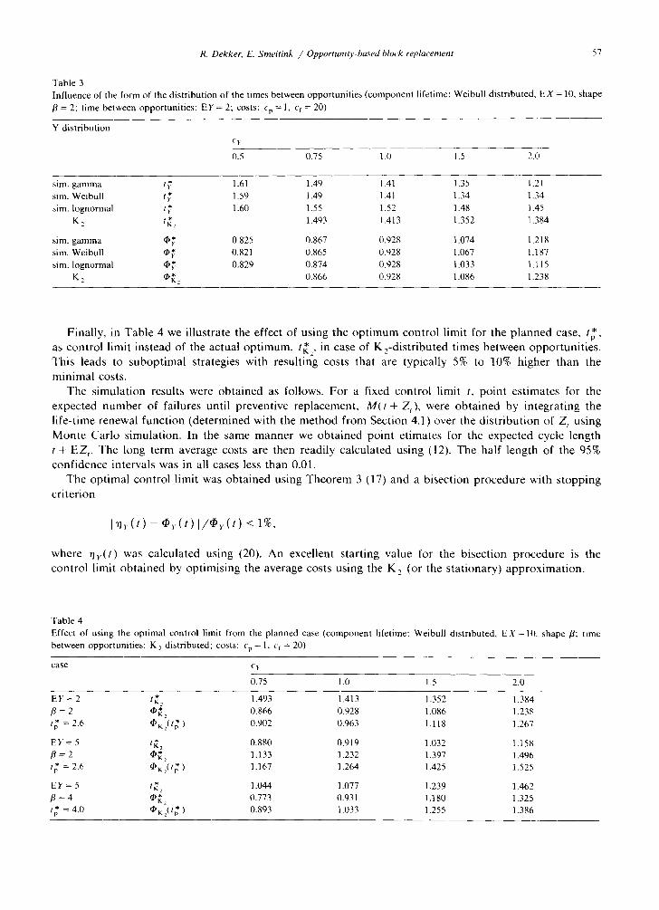
Table 3 Influence of the form of the distribution of the times between opportunities (component lifetime: Weibull distributed, EX = 10, shape /3 = 2; time between opportunities: EY = 2; costs: Cp = 1, cf = 20)

Y distribution Cy

0.5 0.75 1.0 1.5 2.0

sim. gamma t~ 1.61 1.49 1.41 135 1.21 sim. Weibull t~ 1.59 1.49 1.41 1.34 1.34 sire. Iognormal t~ 1.60 1.55 1.52 1.48 1.45

K 2 t * 1.493 1.413 1.352 1.384 K2

sire. gamma q~ 0.825 0.867 0.928 1.074 1.218 sim. Weibull ~ , 0.821 0.865 0.928 1.067 1.187 sim. Iognormal ~ 0.829 0.874 0.928 1.033 1.115

K ~ 4 " 0.866 0.928 1.086 1.238 K 2

Fina l ly , in T a b l e 4 we i l l u s t r a t e the e f fec t of u s i n g t h e o p t i m u m c o n t r o l l imi t for t he p l a n n e d case , t p ,

as c o n t r o l l imi t i n s t e a d of the a c t u a l o p t i m u m , t * in case of K z - d i s t r i b u t e d t i m e s b e t w e e n o p p o r t u n i t i e s . K2~

T h i s l eads to s u b o p t i m a l s t r a t eg i e s w i t h r e s u l t i n g cos t s t h a t a re t yp i ca l l y 5% to 10% h i g h e r t h a n t he

m i n i m a l cos ts .

T h e s i m u l a t i o n r e su l t s we re o b t a i n e d as fo l lows. F o r a f ixed c o n t r o l l imi t t, p o i n t e s t i m a t e s for the

e x p e c t e d n u m b e r o f fa i lu res u n t i l p r e v e n t i v e r e p l a c e m e n t , M ( t + Z,) , were o b t a i n e d b y i n t e g r a t i n g t he

l i f e - t ime r e n e w a l f u n c t i o n ( d e t e r m i n e d w i t h the m e t h o d f r o m S e c t i o n 4,1) o v e r t he d i s t r i b u t i o n of Z, u s i n g

M o n t e C a r l o s i m u l a t i o n . In t he s a m e m a n n e r we o b t a i n e d p o i n t e t i m a t e s for the e x p e c t e d cycle l e n g t h

t + E Z , . T h e l o n g t e r m a v e r a g e cos t s a re t h e n r ead i ly c a l c u l a t e d u s i n g (12). T h e h a l f l e n g t h of t he 95%

c o n f i d e n c e i n t e r v a l s w as in all cases less t h a n 0.01.

T h e o p t i m a l c o n t r o l l im i t was o b t a i n e d u s i n g T h e o r e m 3 (17) a n d a b i s e c t i o n p r o c e d u r e w i t h s t o p p i n g

c r i t e r i o n

[ ~ r ( t ) - ~ , , ( t ) [ / ~ v ( t ) < 1%,

w h e r e 0 r ( t ) was c a l c u l a t e d u s i n g (20). A n exce l l en t s t a r t i n g v a l u e for the b i s e c t i o n p r o c e d u r e is t he

c o n t r o l l imi t o b t a i n e d by o p t i m i s i n g t he a v e r a g e cos t s u s i n g the K 2 (o r the s t a t i o n a r y ) a p p r o x i m a t i o n .

Table 4 Effect of using the optimal control limit from the planned case (component lifetime: Weibull distributed, E X - 1 0 . shape /3; time between opportunities: K 2 distributed; costs: % = 1, cf = 20)

case c v

0.75 1.0 1.5 2.0

EY = 2 t * 1.493 1.413 1.352 1.384 K~ fl = 2 q~2 0.866 0.928 1.086 1.238

• = 2.6 tp ~K 2( tr,* ) 0.902 0.963 1.118 1.267

E Y = 5 t * 0.880 0.919 1.032 1.158 K2 /3 = 2 q~* 1.133 1.232 1.397 1.496 K2

• = 2.6 f19K2(l ~ ) 1.167 1.264 1.425 1.525 lp

EY = 5 t * 1.044 1.077 1.239 1.462 K2 /3 = 4 q~* 0.773 0.931 1 Ago 1.325 K2 tp = 4.0 ~K2( t~ ) 0.893 1.033 1.255 1.386

58 R. Dekker, E. Smeitink / Opportunity-based block replacement

Conclusions from the tables

(1) With the K~ distribution the forward recurrence time distribution can be satisfactory approximated 2 for a wide class of (continuous and unimodal) distributions (with c r > ½). For distributions of the time

between opportunities with c2r ~ ½ the stationary approximation can be used, provided that the ratio E Y / E X is not too large. It is difficult to give a good rule of thumb, but when E Y / E X was between 0 and 0.2 the resulting error made by the stationary approximation was very small in our experiments (see Tables 1 and 2).

(2) Our approximations yield computationally tractable results that outperform a simple strategy such as using the optimal control limit tp for the planned case (see Table 4).

(3) The minimum average costs ~ and the optimal control limit t~ depend substantially on the mean EY and coefficient of variation cr of the time between opportunities (see Table 1 and 2). ~b~ increases with EY and cr, while t~ decreases with EY and can either increase or decrease with c r. The type of distribution is of far less importance, especially for low coefficients of variation (see Table 3).

(4) The approximation of ~b~ by ~* yields errors less than 2% for gamma and Weibuli distributions. Kz For the Iognormal distribution the error remains small (< 5%) in case c r < 1.5. The approximation of ~b~ by ~b~t*at is slightly worse than the approximation by ~b~, but satisfactory for values of cr between 0.25 and 1.5. Both approximations are best for low values of E Y / E X and values of cr that are close to 1.

(5) The errors made in approximating t~ by either t~, or tstat can be large, e.g. up to 50% for tstat and 20% for t~2 in the (extreme) cases with c r = 2. However, as the average cost curves are quite flat around their minimum the error in the average costs resulting from the use of these approximations is much smaller.

5. Extensions

There are a number of ways in which the previous theory can be extended. First of all, we will show that block replacement can also be extended to multiple components. Secondly, one-opportunity-look-ahead policies can be used in setting priorities for execution of maintenance packages if only a limited number of these can be executed at a given opportunity. The latter case will be treated in a subsequent paper.

5. l. Extension of the OBRP to a multicomponent case

So far we have considered one component only. In practice, maintenance activities involving replace- ment of components are usually combined into a maintenance package. When executed preventively, always the whole package is carried out, whereas upon failure, only the failed component is replaced. The problem then is to determine the optimal control limit for execution of the maintenance package. The extension of the OBRP model to a multi-component case is straightforward. Notice that the entire analysis of Sections 2 and 3 can be applied. The only change required in the formulas is that we have to distinguish n possibly different components. For example, in the formula for q~r(t) we replace c fM( t ) by

n

E c~i'M,( t ) i = 1

where the index i indicates component i. Analogous changes have to be made in the other formulas. All the results remain valid, only in Theorem 3 we require that

(o2) Cp<½ c~ ~) 1 - - ~

i=l /~J (28)

R. Dekker, E. Smeitink / Opportunitv-based block replacement 59

instead of condition (18), and furthermore that t l

I2 cl"m,(t) (29) i = l

must be increasing (instead of re(t)). Similar problems as mentioned in Remark 2 with respect to the increase of m(t) are encountered in the last condition. If the component lifetimes are quite different it poses severe problems as there may be multiple minima and the first minimum does not need to be the absolute minimum.

Appendix 1. Proof of Lemma 2.

The main difficulty is to show that the order of integration and differentiation may be interchanged. To use a standard theorem of analysis (see e.g. [1]) we have to make the following three observations.

(1) The integral f~rn(t + z){1 - q'(t, z)} dz is convergent on [0, oc). This follows from the fact that m(. ) allows majoration by a constant and EZ t is finite for every t > 0. The majoration of m(.) follows from the renewal density theorem and the continuity of m(.).

(2) The function (d/dt)m(t + z){1 - gift, z)} is continuous on [0, oc) × [0, oc). This follows directly from the assumption that m( . ) is continuously differentiable and (9) combined

with the assumption that G(-) and n( . ) are continuously differentiable. (3) The integral

converges uniformly in t on [0, oc). To see this we write

=Y0 d ~'{1-'t '(t ,z)}~m(t+z)dz+ m(t+z)N{1- ' t ' ( t ,z)}dz

= { 1 - q t ( t , N)}m(t+N)- {1-qs(t,O)}m(t)

- Xm(t+zl~z { l - q t ( t , : )} d z + Nrn(t+z)N

= { 1 - * ( t , U))m(t+N)- { 1 - g ' ( t , 0 ) } m ( t )

+ ~Nm(t+ z){ "~--~qt(t, z ) - a ~- ' / ' ( t , z)} dz. (31)

From (9) it follows that

3 a ~ q, ( t , z ) - ~ q , ( t , z ) = (1 - C(z)}~(t).

Hence, using (31) we can write

£ d{m(,+zl l-*t,,z)lldz fo N ={l-e(t,N)}m(t+N)-{l- ' t '(t ,O)}m(t)+EYn(t) m(l+z)dP(Z~z).

(32)

60 R. Dekker, E. Smeitink / Opportunity-based block replacement

It is easy to show that 9(t, z) converges uniformly to 9(z). Now with (32) and the finiteness of EZ it

follows that (30) converges uniformly on [0, cc). Having made these three observations, we can use Theorem 14-24 (p. 443) of [l] to change the order of integration and differentiation and with (32) we

obtain, noting that \k(t, 0) = 0,

= EYn(t)i ?~(r+z) dP(Z<z)

which concludes the proof. 0

Appendix 2

In this appendix we give definitions of the Weibull and K, distributions and derive the distribution of

the forward recurrence time Z,, P( Z, d z) for phase type distributions. For the K, distribution we derive

an analytical expression for P(Z, d z).

Definition of the Weibull distribution

A random variable X has a Weibull distribution with scale parameter h and shape parameter p if its

probability density function satisfies

f(t)=i~/Q1exp(-(~!B), ta0.

Definition of the K2 distribution

A random variable X has a K, distribution if

x= 1

Xl with probability p,

x, + x, with probability 1 - p,

where X, and X, are independent and exponentially distributed with parameters X, and hz, respectively

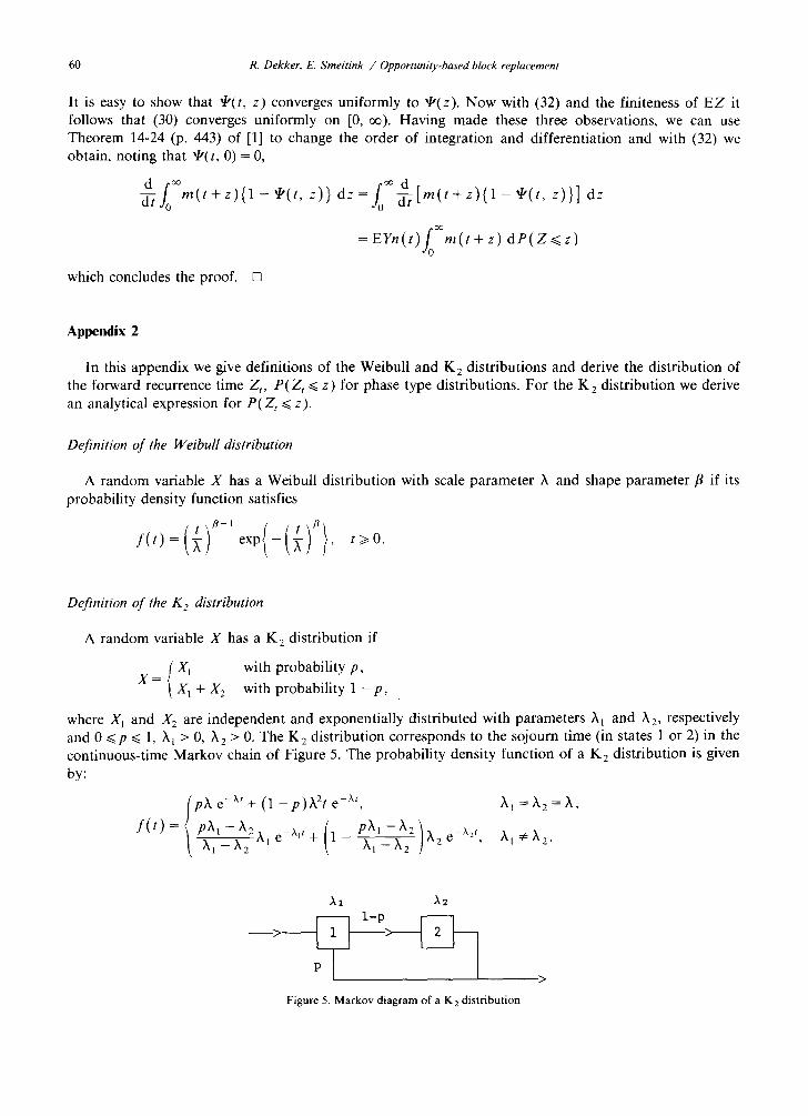
and 0 bp G 1, A, > 0, A, > 0. The K, distribution corresponds to the sojourn time (in states 1 or 2) in the continuous-time Markov chain of Figure 5. The probability density function of a K, distribution is given

by:

(ph e-” + (1 -p)A2t eCAr, A, =h,=X,

f(t) = PA, -A,

\ x

1 _ x A, ePX1’ + 1 - p~1~~2

2 ( 1

2 X, eeX2’, X, ZX,. i

Figure 5. Markov diagram of a K, distribution

R. Dekker, E. Smeitink / Opportunity-based block replacement 61

Fitt ing a K 2 distribution on the first two moments leaves some degree of f reedom in the choice of the parameters ?t 1, X 2 and p. In some cases the third momen t can also be fitted, but this is not always possible. A good alternative is to use a gamma normalisat ion to obtain a unique fit. This means that ?t~, ?t 2 and p are chosen in such a way that the third moment of the K 2 distr ibution equals the third moment of a gamma distribution with the same first and second moment as X. This is always possible (see also [21, pp.

399-400]) and X~, X 2 and p are given by

2 2 1 't 4 C X - ~ I 1/2

+ c -;TJ l' x -Ex ~k 2

p = (1 - 2t2EX) + ~ - 1 •

The distribution of the forward recurrence time for PH-distributions

Consider a continuous-t ime Markov chain with state space {1 . . . . . m + 1}. States 1 . . . . . m are transient and state m + 1 is absorbing. The infinitesimal generator Q of such a Markov chain has the form

where T is a nonsingular m x m matrix and T O is an m-vector. Matrix T has ~i < 0, for 1 ~< i ~< m, and T,j >/0 for i ~ j . Vector T O >i 0 satisfies Te + T O = 0 where e ' = (1 . . . . . 1). Let (a, am+l) denote the vector of initial probabilities, where a is an m vector such that 0 < ae ~< 1. The distribution G of the time until absorpt ion in state m + 1 given the initial probabil i ty vector (a, a m + 1) is

G ( x ) = l - a e x p ( T x ) e , x>lO. (33)

A distribution G defined by (33) is called a phase-type distribution (PH distribution). The pair (a, T) is called the representation of G. If the Markov process is restarted instantaneously after each absorpt ion into state m + 1 and if each process restart is considered a renewal, then the interrenewal time distribution is the PH distribution (33). Such a process is called a phase-type renewal process and its infinitesimal generator is given by

Q * = T + ( 1 - a m + l ) - Z T ° a .

A direct and very useful analogon of Lemma 2.2.2 in Neuts [13, pp. 45] is the following lemma.

Lemma 7. The probability distribution P( Z t <~ z) of the forward recurrence time, corresponding to the PH distribution with representation ( a, T) is given by

P ( Z , < ~ z ) = l - a e x p ( Q * t ) exp(Tz)e , t, z>~O. (34)

Proof. The uncondit ional probabilities wj(t) that the PH-renewal process is in state j at time t, j = 1 . . . . . m, satisfy the system of differential equations

w ' ( t ) = w ( t ) Q * ,

with initial condit ions w(0) = a. Its solution is given by

w( t ) = a e x p ( Q * t ) .

Clearly, P (Z , ~< z) is a PH distribution with representation (w(t) , T). []

62 R. Dekker, E. Smeitink / Opportunity-based block replacement

Let ~b(t, z) and qJ(z) denote the probability density function of Z, and Z respectively. The following statements are readily verified from Lemma 7 respectively (11):

0 ~ ( t , z ) = -~-z q'(t , z ) = a exp(Q*t ) exp(Tz)r °, (35)

EZ, = - a exp(Q*t)T 'e, (36)

P ( Y > z ) EY 2 ~b(z) EY ' E Z = 2EY" (37)

The distribution of the forward recurrence time of a K 2 distribution

With (34) an analytic expression for distribution we have

T= 0 -?t2 , X2 , a = (1, 0),

and the generator of the associated PH-renewal process is given by

= ( - ( 1 - P ) A ' Q* ~2

After some calculus we obtain

A2 w,(t) = Xl(1 _ p ) + X2

and

(1 -p)X~) __)k 2

• (t, z) for the K 2 distribution is easily obtained. For the K 2

X~(1 - p ) e_{X,~l_p)+x~} ' X~(1 - p ) +X2

p)k I - ~,2 e_~,,~ (1 - P ) ~ I ) exp(Tz)e ~ --~-£ + X ; ~ - 2 e-X2z = ' ~1 :::# )k2 '

e-X2z

exp(Tz)e e-X: + (1 - P ) ) t z e-X;) = X 1 = X 2 = X . e_XZ

Now we can write

P(Z, <~ z) = 1 - (w,( t) , 1 - wl(t)) exp(Tz)e

i P)~I - X2 x [ P)~1- X2 = - w , ( t ) - x T ~ - f e - ' : - [ 1 - w l ( t ) -~12ZX2 l e ~ ,

e -x" - w,(t)(1 - p ) ) t z e -xz,

X 1:7/= )k2,

)k 1 = A 2 = A .

(38)

Remark. For any K 2 distribution the curve of ~p(t, z) intersects +(z) in the same point z c independently of t, which is given by

{ log(?~l ) - l og ( •2 ) z = X l _ X z , X 14=x2,

l / h , ?t I = ,k 2 = ),.

The probability density ~(t , z) and EZ, are easily obtained from (38) (or directly from (35) resp. (36), using a exp(Q*t) = (wl(t), 1 - wl(t)) ). Let ~(z ) denote the probability density function of Z. In Figure 3

2 = 2 . we plotted the probability densities ~p(t, z) and ~b(z) for c~ = ½ and cv

R. Dekker, E. Smeitink / Opportunity-based block replacement 63

Acknowledgements

The au tho r s like to t hank M a r c e l van der Lee and T h e o M a n d o s for c a r r y i n g o u t the s i m u l a t i o n s tudies

r e p o r t e d in this paper .

References

[1] Apostol, T.M., Mathematical Analysis: A Modern Approach to Advanced Calculus. Addison-Wesley Publishing Company, 1965. [2] B~ickert. W., and Rippin, D,W.T., "The determination of maintenance strategies for plants subject to breakdown", Computers

and Chemical Engineering 9 (1985) 113-126. [31 Barlow, R.E., and Proschan, F., Mathematical Theory of Reliability, Wiley, New York, 1965. [4] Berg, M., "General trigger-off replacement procedures for two-unit systems", Naval Research Logistics Quarterly 25 (1978)

15-29. [5] Berg, M.. "A marginal cost analysis for preventive maintenance policies", European Journal of Operational Research, 4 (1980)

136 142. [6] Berg, M., and Epstein, B., "A modified block replacement policy", Naval Research Logistics Quarterl), 23 (1976) 15-24. [7] Dekker, R., and Dijkstra, M.C., "Opportunity based age replacement", to appear in Naoal Research Logistics. [8] Duncan, J.. and Scholnick, L.S., "Interrupt and opportunistic replacement strategies for systems of deteriorating components",

Operational Research Quarterly 24 (1973) 271-283. [9] Giblim M.T., "Derivation of renewal functions using discretisation", in: 8th Advances in Reliability Techniques Symposium, 1984,

[10] Hanscom, M.A., and Cleroux, R., "The block replacement problem", Journal of Statistical Computations and Simulations 3 (1975) 233 248.

[11] Jorgensem D.W.. McCall, J.J., and Radner. R., Optimal Replacement Polky, North-Holland, Amsterdam, 1967. [12] Liang, T.Y., "Optimum piggyback preventive maintenance policies", IEEE Transactions on Reliability 34 (1985~ 529-538. [13] Neuts. M.F., Matrix-Geometric Solutions in Stochastic Models. Johns Hopkins University Press, Baltimore, MD, 1981. [141 Pierskalla, W.P., and Voelker, J.A., "A survey of maintenance models: The control and surveillance of deteriorating systems",

Naeal Research Logistics Quarterly 23 (1976) 353-388. [15] Ross, S.M., Applied Probability Models with Optimization Applications, Holden-Day, San Fransisco, 1970. [16] Sethi, D.P.S., "'Opportunistic Replacement Policies", in I.N. Shimi & C.P. Tsokos (eds.), The Theory and Applications of

Reliability, Vol. 1, Academic Press, New York, 1977, 433-447. [17] Sherif, Y.S., and Smith, M.L., "Optimal maintenance models for systems subject to failure - a review", Naval Researeh Logisties

Quarterly 28 (1981) 47-74. [18] Sherif, Y.S., "Reliability analyses. Optimal inspection and maintenance schedules for failing systems", Mieroeleetronics

Reliability 22 (1982) 59-115. [19] Smeitink, E., and Dekker, R., "A simple approximation to the renewal function", IEEE Transactions on Reliability 39 (1990)

71 75. [20] Stroud, A.H., and Secrest, D., Gaussian Quadrature Formulas, Prentice-Hall, Englewood Cliffs (1966). [21] Tijms, H.C., Stochastic Modelling and Analysis: A Computational Approach, John Wiley, New York, 1986. [221 Woodman, R.C., "Replacement policies for components that deteriorate", Operational Research Quarterly 18 (1967) 267-280.