Operations Research OPERATION WWW.CHKBUJJI.WEEBLY.COM , RESEARCH Subject Code No. of Lecture Hrs./ Week Total No. of Lecture Hrs. : 06CS661 : 04 : 52 IA Marks : 25 Exam Hours : 03 Exam Marks : 100 UNIT - 1 INTRODUCTION: Linear programming, Definition, scope of Operations Research (O.R) approach and limitations of OR Models, Characteristics and phases of OR Mathematical formulation of L.P. Problems. Graphical solution methods. 6 Hours UNIT - 2 LINEAR PROGRAMMING PROBLEMS: The simplex method - slack, surplus and artificial variables. Concept of duality, two phase method, dual simplex method, degeneracy, and procedure for resolving degenerate cases. 7 Hours\ UNIT - 3 TRANSPORTATION PROBLEM: Formulation of transportation model, Basic feasible solution using different methods, Optimality Methods, Unbalanced transportation problem, Degeneracy in transportation problems, Applications of Transportation problems. Assignment Problem: Formulation, unbalanced assignment problem, Traveling salesman problem. 7 Hours UNIT - 4 SEQUENCING: Johnsons algorithm, n - jobs to 2 machines, n jobs 3machines, n jobs m machines without passing sequence. 2 jobs n machines with passing. Graphical solutions priority rules. 6 Hours PART - B UNIT – 5 QUEUING THEORY: Queuing system and their characteristics. The M/M/1 Queuing system, Steady state performance analysing of M/M/ 1 and M/M/C queuing model. 6 Hours Department of CS&E WWW.CHKBUJJI.WEEBLY.COM

Welcome message from author
This document is posted to help you gain knowledge. Please leave a comment to let me know what you think about it! Share it to your friends and learn new things together.
Transcript

Operations Research
OPERATION
WWW.CHKBUJJI.WEEBLY.COM ,
RESEARCH
Subject Code
No. of Lecture Hrs./ Week
Total No. of Lecture Hrs.
: 06CS661
: 04
: 52
IA Marks : 25
Exam Hours : 03
Exam Marks : 100
UNIT - 1
INTRODUCTION: Linear programming, Definition, scope of Operations Research (O.R) approach
and limitations of OR Models, Characteristics and phases of OR Mathematical formulation of L.P.
Problems. Graphical solution methods. 6 Hours
UNIT - 2
LINEAR PROGRAMMING PROBLEMS: The simplex method - slack, surplus and artificial
variables. Concept of duality, two phase method, dual simplex method, degeneracy, and procedure for
resolving degenerate cases. 7 Hours\
UNIT - 3
TRANSPORTATION PROBLEM: Formulation of transportation model, Basic feasible solution using
different methods, Optimality Methods, Unbalanced transportation problem, Degeneracy in
transportation problems, Applications of Transportation problems. Assignment Problem: Formulation,
unbalanced assignment problem, Traveling salesman problem. 7 Hours
UNIT - 4
SEQUENCING: Johnsons algorithm, n - jobs to 2 machines, n jobs 3machines, n jobs m machines
without passing sequence. 2 jobs n machines with passing. Graphical solutions priority rules.
6 Hours
PART - B
UNIT – 5
QUEUING THEORY: Queuing system and their characteristics. The M/M/1 Queuing system, Steady
state performance analysing of M/M/ 1 and M/M/C queuing model. 6 Hours
Department of CS&E
WWW.CHKBUJJI.WEEBLY.COM

Operations Research WWW.CHKBUJJI.WEEBLY.COM
UNIT - 6
PERT-CPM TECHNIQUES: Network construction, determining critical path, floats, scheduling by
network, project duration, variance under probabilistic models, prediction
crashing of simple networks.
of date of completion,
7 Hours
UNIT - 7
GAME THEORY: Formulation of games, Two person-Zero sum game, games with and without saddle
point, Graphical solution (2x n, m x 2 game), dominance property. 7 Hours
UNIT - 8
INTEGER PROGRAMMING: Gommory’s programming problems, zero one algorithm
technique, branch and bound lgorithm for integer
6 Hours
TEXT BOOKS:
1. Operations Research and Introduction, Taha H. A. – Pearson Education edition
2. Operations Research, S. D. Sharma –Kedarnath Ramnath & Co 2002.
REFERENCE BOOKS:
1. “Operation Research” AM Natarajan, P. Balasubramani, A Tamilaravari Pearson 2005
2. Introduction to operation research, Hiller and liberman, Mc Graw Hill. 5th edition 2001.
3. Operations Research: Principles and practice: Ravindran, Phillips & Solberg, Wiley India lts,
2nd Edition 2007
4. Operations Research, Prem Kumar Gupta, D S Hira, S Chand Pub, New Delhi, 2007
Department of CS&E
WWW.CHKBUJJI.WEEBLY.COM
Operations Research [06CS661] WWW.CHKBUJJI.WEEBLY.COM
TABLE OF CONTENTS
1. INTRODUCTION, FORMULATION OF LPP - 03 - 20
2. LINEAR PROGRAMMING PROBLEMS, SIMPLEX METHOD - 21 – 37
3. TRANSPORTATION PROBLEM - 38 - 57
4. QUEUING THEORY - 58 – 74
5. PERT-CPM TECHNIQUES - 75 - 85
6. GAME THEORY - 86 – 93
7. INTEGER PROGRAMMING - 94 - 98
Department of CS&E
WWW.CHKBUJJI.WEEBLY.COM
Operations Research [06CS661] WWW.CHKBUJJI.WEEBLY.COM
INTRODUCTION
Operations research, operational research, or simply OR, is the use of mathematical models,
statistics and algorithms to aid in decision-making. It is most often used to analyze complex real-world
systems, typically with the goal of improving or optimizing performance. It is one form of applied
mathematics.
The terms operations research and management science are often used synonymously. When a
distinction is drawn, management science generally implies a closer relationship to the problems of
business management.
Operations research also closely relates to industrial engineering. Industrial engineering takes
more of an engineering point of view, and industrial engineers typically consider OR techniques to be a
major part of their toolset.
Some of the primary tools used by operations researchers are statistics, optimization, stochastics,
queueing theory, game theory, graph theory, and simulation. Because of the computational nature of
these fields OR also has ties to computer science, and operations researchers regularly use custom-
written or off-the-shelf software.
Operations research is distinguished by its ability to look at and improve an entire system, rather
than concentrating only on specific elements (though this is often done as well). An operations researcher
faced with a new problem is expected to determine which techniques are most appropriate given the
nature of the system, the goals for improvement, and constraints on time and computing power. For this
and other reasons, the human element of OR is vital. Like any tools, OR techniques cannot solve
problems by themselves.
Areas of application
A few examples of applications in which operations research is currently used include the following:
designing the layout of a factory for efficient flow of materials
constructing a telecommunications network at low cost while still guaranteeing quality
service if particular connections become very busy or get damaged
determining the routes of school buses so that as few buses are needed as possible
designing the layout of a computer chip to reduce manufacturing time (therefore reducing
cost)
managing the flow of raw materials and products in a supply chain based on uncertain
demand for the finished products
Department of CS&E Page 3
WWW.CHKBUJJI.WEEBLY.COM

Operations Research [06CS661] WWW.CHKBUJJI.WEEBLY.COM
Unit –I
Introduction & Formulation of LPP
Define OR
OR is the application of scientific methods, techniques and tools to problems involving the operations of
a system so as to provide those in control of the system with optimum solutions to the problems.
Characteristics of OR
1. its system orientation
2. the use of interdisciplinary teams
3. application of scientific method
4. uncovering of new problems
5. improvement in the quality of decisions
6. use of computer
7. quantitative solutions
8. human factors
1. System (or executive) orientation of OR
production dept.: Uninterrupted production runs, minimize set-up and clean-up costs.
marketing dept.: to meet special demands at short notice.
finance dept.: minimize inventories should rise and fall with rise and fall in company’s sales.
personnel dept.: maintaining a constant production level during slack period.
2. The use of interdisciplinary teams.
Psychologist: want better worker or best products.
Mechanical Engg.: will try to improve the machine.
Software engg.: updated software to sole problems.
that is, no single person can collect all the useful scientific information from all disciplines.
3. Application of scientific method
Most scientific research, such as chemistry and physics can be carried out in Lab under controlled
condition without much interference from the outside world. But this is not true in the case of OR
study.
An operations research worker is the same position as the astronomer since the latter can be observe
the system but cannot manipulate.
Department of CS&E Page 4
WWW.CHKBUJJI.WEEBLY.COM

Operations Research [06CS661] WWW.CHKBUJJI.WEEBLY.COM
4. Uncovering of new problems
In order to derive full benefits, continuity research must be maintained. Of course, the results of OR
study pertaining a particular problem need not wait until all the connected problems are solve.
5. Improvement in the Quality of decision
OR gives bad answer to problems, otherwise, worst answer are given. That is, it can only improve
the quality of solution but it may not be able to give perfect solution.
6. Use of computer
7. Quantitative solutions
for example, it will give answer like, “the cost of the company, if decision A is taken is X, if
decision B is take is Y”.
8. Human factors.
Scope of Operation Research
1) Industrial management:
a) production b) product mix c) inventory control d) demand e) sale and purchase f) transportation
g) repair and maintenance h) scheduling and control
2) Defense operations:
a) army b) air force c) navy
all these further divided into sub-activity, that is, operation, intelligence administration, training.
3) Economies:
maximum growth of per capita income in the shortest possible time, by taking into consideration the
national goals and restrictions impose by the country. The basic problem in most of the countries is
to remove poverty and hunger as quickly as possible.
4) Agriculture section:
a) with population explosion and consequence shortage of food, every country is facing the problem
of optimum allocation land to various crops in accordance with climatic conditions.
b) optimal distribution of water from the various water resource.
5) Other areas:
a) hospital b) transport c) LIC
Department of CS&E Page 5
WWW.CHKBUJJI.WEEBLY.COM
Operations Research [06CS661] WWW.CHKBUJJI.WEEBLY.COM
Phases of OR
1) Formulating the problem
in formulating a problem for OR study, we mist be made of the four major components.
i) The environment
ii) The decision maker
iii) The objectives
iv) Alternative course of action and constraints
2) Construction a Model
After formulating the problem, the next step is to construct mode. The mathematical model consists
of equation which describes the problem.
the equation represent
i) Effectiveness function or objective functions
ii) Constraints or restrictions
The objective function and constraints are functions of two types of variable, controllable variable
and uncontrollable variable.
A medium-size linear programming model with 50 decision variable and 25 constraints will have
over 1300 data elements which must be defined.
3) Deriving solution from the model
an optimum solution from a model consists of two types of procedure: analytic and numerical.
Analytic procedures make use of two types the various branches of mathematics such as calculus or
matrix algebra. Numerical procedure consists of trying various values of controllable variable in the
mode, comparing the results obtained and selecting that set of values of these variables which gives
the best solution.
4) Testing the model
a model is never a perfect representation of reality. But if properly formulated and correctly
manipulated, it may be useful predicting the effect of changes in control variable on the over all
system.
5) Establishing controls over solution
a solution derived from a model remains a solution only so long as the uncontrolled variable retain
their values and the relationship between the variable does not change.
6) Implementation
OR is not merely to produce report to improve the system performance, the result of the research
Department of CS&E Page 6
WWW.CHKBUJJI.WEEBLY.COM

Operations Research [06CS661] WWW.CHKBUJJI.WEEBLY.COM
must implemented.
Additional changes or modification to be made on the part of OR group because many time solutions
which look feasible on paper may conflict with the capabilities and ideas of persons.
Limitations of OR
1) Mathematical models with are essence of OR do not take into account qualitative factors or
emotional factors.
2) Mathematical models are applicable to only specific categories of problems
3) Being a new field, there is a resistance from the employees the new proposals.
4) Management may offer a lot of resistance due to conventional thinking.
5) OR is meant for men not that man is meant for it.
Difficulties of OR
1) The problem formulation phase
2) Data collection
3) Operations analyst is based on his observation in the past
4) Observations can never be more than a sample of the whole
5) Good solution to the problem at right time may be much more useful than perfect solutions.
Department of CS&E Page 7
WWW.CHKBUJJI.WEEBLY.COM

Operations Research [06CS661] WWW.CHKBUJJI.WEEBLY.COM
Linear Programming
Requirements for LP
1. There must be a well defined objective function which is to be either maximized or minimized and
which can expressed as a linear function of decision variable.
2. There must be constraints on the amount of extent of be capable of being expressed as linear
equalities in terms of variable.
3. There must be alternative course of action.
4. The decision variable should be inter-related and non-negative.
5. The resource must be limited.
Some important insight:
• The power of variable and products are not permissible in the objective function as well as
constraints.
• Linearity can be characterized by certain additive and multiplicative properties.
Additive example :
If a machine process job A in 5 hours and job B in 10 hours, then the time taken to process both job
is 15 hours. This is however true only when the change-over time is negligible.
Multiplicative example:
If a product yields a profit of Rs. 10 then the profit earned fro the sale of 12 such products will be
Rs( 10 * 12) = 120. this may not be always true because of quantity discount.
• The decision variable are restricted to have integral values only.
• The objective function does not involve any constant term.
that is, z = ∑c
j x j + c , that is, the optimal values are just independent of any constant c. j =1
Department of CS&E Page 8
WWW.CHKBUJJI.WEEBLY.COM

Operations Research [06CS661] WWW.CHKBUJJI.WEEBLY.COM
Examples on Formulation of the LP model
Example 1: Production Allocation Problem
A firm produces three products. These products are processed on three different machines. The time
required to manufacture one unit of each of the product and the daily capacity of the three machines are
given in the table below.
Machine
Time per unit(minutes
Product 1 Product 2 Product 3
Machine capacity
(minutes/day)
M1 2 3 2 440
M2 4 --- 3 470
M3 2 5 --- 430
It is required to determine the daily number of units to be manufactured for each product. The profit per
unit for product 1,2 and 3 is Rs. 4, Rs. 3 and Rs. 6 respectively. It is assumed that all the amounts
produced are consumed in the market.
Formulation of Linear Programming model
Step 1: The key decision to be made is to determine the daily number of units to be manufactured for
each product.
Step 2: Let x1, x2 and x3 be the number of units of products 1,2 and 3 manufactured daily.
Step 3: Feasible alternatives are the sets of values of x1, x2 and x3 where x1,x2,x3 ≥ o. since negative
number of production runs has no meaning and is not feasible.
Step 4: The objective is to maximize the profit, that is , maximize Z = 4x1 + 3x2 + 6x3
Step 5: Express the constraints as linear equalities/inequalities in terms of variable. Here the constraints
are on the machine capacities and can be mathematically expressed as,
2x1 + 3x2 + 2x3 ≤ 440,
4x1 + 0 x2 + 3x3 ≤ 470
2x1 + 5x2 + 0x3 ≤ 430 Department of CS&E Page 9
WWW.CHKBUJJI.WEEBLY.COM

Operations Research [06CS661] WWW.CHKBUJJI.WEEBLY.COM
Example 2: Advertising Media Selection Problem.
An advertising company whishes to plan is advertising strategy in three different media – television,
radio and magazines. The purpose of advertising is to reach as large as a number of potential customers
as possible. Following data has been obtained from the market survey:
Cost of an
advertising unit
No of potential
customers
reached per unit
No. of female
customers
reached per unit
Television
Rs. 30,000
2,00,000
1,50,000
Radio
Rs. 20,000
6,00,000
4,00,000
Magazine 1
Rs. 15,000
1,50,000
70,000
Magazine 2
Rs. 10,000
1,00,000
50,000
The company wants to spend not more than Rs. 4,50,000 on advertising. Following are the further
requirement that must be met:
i) At least 1 million exposures take place among female customers
ii) Advertising on magazines be limited to Rs. 1,50,000
iii) At least 3 advertising units be bought on magazine I and 2 units on magazine II &
iv) The number of advertising units on television and radio should each be between 5 and 10
Formulate an L.P model for the problem.
Solution:
The objective is to maximize the total number of potential customers.
That is, maximize Z = (2x1 + 6x2 + 1.5x3 + x4) * 105
Constraints are
On the advertising budget
On number of female
On expense on magazine
On no. of units on magazines
On no. of unit on television
Department of CS&E
30,000x1 + 20,000x2 + 15,000x3 + 10,000x4 ≤ 4,50,000
1,50,000x1 + 4,00,000x2 + 70,000x3 + 50,000 x4 ≥ 10,00,000
15,000x3 + 10,000x4 ≤1,50,000
x3≥ 3, x4 ≥ 2
5 ≤ x2 ≤ 10, 5 ≤ x2 ≤10
Page 10
WWW.CHKBUJJI.WEEBLY.COM

Operations Research [06CS661] WWW.CHKBUJJI.WEEBLY.COM
Example 3 :
A company has two grades of inspectors, 1 and 2 to undertake quality control inspection. At least 1,500
pieces must be inspected in an 8 hour day. Grade 1 inspector can check 20 pieces in an hour with an
accuracy of 96%. Grade 2 inspector checks 14 pieces an hour with an accuracy of 92%.
The daily wages of grade 1 inspector are Rs. 5 per hour while those of grade inspector are Rs. 4 per
hour, any error made by an inspector costs Rs. 3 to the company. If there are, in all, 10 grade 1
inspectors and 15 grade 2 inspectors in the company, find the optimal assignment of inspectors that
minimize the daily inspection cost.
Solution
Let x1, x2 be the inspector of grade 1 and 2.
Grade 1: 5 + 3 * 0.04 * 20
Grade 2: 4 + 3 * 0.08 * 14
Z = 8*(7.4x1 + 7.36x2)
X1 ≤ 10, x2 ≤ 15
20 * 8 x1 + 14* 8 x2 ≥ 1500
Example 4:
An oil company produces two grades of gasoline P and Q which it sells at Rs. 3 and Rs.4 per litre. The
refiner can buy four different crude with the following constituents an costs:
Crude Constituents Price/litre
A B C
1 0.75 0.15 0.10
2 0.20 0.30 0.50
3 0.70 0.10 0.20
4 0.40 0.60 0.50
Rs. 2.00
Rs. 2.25
Rs. 2.50
Rs. 2.75
The Rs. 3 grade must have at least 55 percent of A and not more than 40% percent of C. The Rs. 4 grade
must not have more than 25 percent of C. Determine how the crude should be used so as to maximize
profit.
Solution:
Let x1p – amount of crude 1 used for gasoline P
Department of CS&E Page 11
WWW.CHKBUJJI.WEEBLY.COM

Operations Research [06CS661] WWW.CHKBUJJI.WEEBLY.COM
x2p – amount of crude 2 used for gasoline P
x3p – amount of crude 3 used for gasoline P
x4p – amount of crude 4 used for gasoline P
x1q – amount of crude 1 used for gasoline Q
x2q – amount of crude 2 used for gasoline Q
x3q – amount of crude 3 used for gasoline Q
x4q – amount of crude 4 used for gasoline Q
The objective is to maximize profit.
that is, 3(x1p+x2p+x3p+x4p) 4 (x1q+x2q+x3q+x4q) - 2(x1p+x1q) – 2.25 (x2p + x2q) – 2.50 (x3p + x3q) – 2.75
(x4p + x4q)
that is, maximize Z = x1p+0.75x2p+0.50x3p+0.25x4p+2x1q+1.75x2q+1.50x3q+1.25x4q
The constraints are:
0.75x1p+0.20x2p+.70x3p+0.40x4p ≥ 0.55(x1p+x2p+x3p+x4p),
0.10x1p+0.50x2p+0.20x3p+0.50x4p ≤ 0.40(x1p+x2p+x3p+x4p),
0.10x1q+0.50x2q+0.20x3q+0.50x4q ≤ 0.25(x1q+x2q+x3q+x4q)
Example 5:
A person wants to decide the constituents of a diet which will fulfill his daily requirements of proteins,
fats and carbohydrates at the minimum cost. The choice is to be made from four different types of foods.
The yields per unit of these foods are given below
Yield per unit Food type
Proteins Fats Carbohydrates
Cost per
unit
1 3 2 6 45
2 4 2 4 40
3 8 7 7 85
4 6 5 4 65
Minimum 800 200 700
requirement
Formulate linear programming model for the problem.
Solution:
The objective is to minimize the cost
That is , Z = Rs.(45x1+40x2+85x3+65x4)
Department of CS&E Page 12
WWW.CHKBUJJI.WEEBLY.COM

Operations Research [06CS661] WWW.CHKBUJJI.WEEBLY.COM
The constraints are on the fulfillment of the daily requirements of the constituents.
For proteins,
For fats,
For carbohydrates,
Example 6:
3x1 + 4x2+8x3+6x4 ≥ 800
2x1 + 4x2+7x3+5x4 ≥ 200
6x1 + 4x2+7x3+4x4 ≥ 700
The strategic border bomber command receives instructions to interrupt the enemy tank production. The
enemy has four key plants located in separate cities, and destruction of any one plant will effectively halt
the production of tanks. There is an acute shortage of fuel, which limits to supply to 45,000 litre for this
particular mission. Any bomber sent to any particular city must have at least enough fuel for the round
trip plus 100 litres.
The number of bombers available to the commander and their descriptions, are as follows:
Bomber type
A
B
Description
Heavy
Medium
Km/litre
2
2.5
Number available
40
30
Information about the location of the plants and their probability of being attacked by a medium bomber
and a heavy bomber is given below:
Plant Distance from base
(km)
Probability of destruction by
A heavy A medium
bomber bomber
A Heavy 2 40
B Medium 2.5 30
How many of each type of bombers should be dispatched, and how should they be allocated among the
four targets in order to maximize the probability of success?
Solution:
Let xij is number of bomber sent.
The objective is to maximize the probability of success in destroying at least one plant and this is
equivalent to minimizing the probability of not destroying any plant. Let Q denote this probability:
then, Q = (1 – 0.1) xA1 . (1 – 0.2) xA2 . (1 – 0.15) xA3. (1 – 0.25) xA4 .
(1 – 0.08) xB1 . (1 – 0.16) xB2 . (1 – 0.12) xB3 . (1 – 0.20) xB4
Department of CS&E Page 13
WWW.CHKBUJJI.WEEBLY.COM

�
�
� 2 2 2 2
� � � � � � �
� � � �
� � � � � � � � � �
Operations Research [06CS661] WWW.CHKBUJJI.WEEBLY.COM
here the objective function is non-linear but it can be reduced to the linear form.
Take log on both side, moreover, minimizing log Q is equivalent to maximizing –log Q or maximizing
log 1/Q
log 1/Q = -(xA1 log 0.9 + xA2 log 0.8 + xA3 log 0.85 + xA4 log 0.75 +
xB1 log 0.92 + xB2 log 0.84 + xB3 log 0.88 + xB4 log 0.80)
therefore, the objective is to maximize
log 1/Q = -(0.0457xA1 + 0.09691 xA2 + 0.07041 xA3 + 0.12483 xA4 +
0.03623xB1 + 0.07572xB2 + 0.05538xB3 + 0.09691xB4)
The constraints are, due to limited supply of fuel
�2 × 400 + 100�× A +
�2×
450 + 100�× A +
�2×
500 + 100�× A +
�2×
600 + 100�× A
+ � � � � � � � �
�2 ×
2.5 +100�×B1 + �
2× 2.5
+100�×B2 + �2× 2.5
+100�×B3 + � 2×
2.5 +100�×B4 ≤ 45,000
that is, 500xA1 + 550 xA2 + 600 xA3 + 700 xA4 +
420xB1 + 460xB2 + 500xB3 + 580xB4 ≤ 45,000
due to limited number of aircrafts,
xA1 + xA2 + xA3 + xA4 ≤40
xB1 + xB2 + xB3 + xB4 ≤ 30
Example 7:
A paper mill produces rolls of paper used cash register. Each roll of paper is 100m in length and can be
produced in widths of 2,4,6 and 10 cm. The company’s production process results in rolls that are 24cm
in width. Thus the company must cut its 24 cm roll to the desired width. It has six basic cutting
alternative as follows:
Department of CS&E Page 14
WWW.CHKBUJJI.WEEBLY.COM
Operations Research [06CS661] WWW.CHKBUJJI.WEEBLY.COM
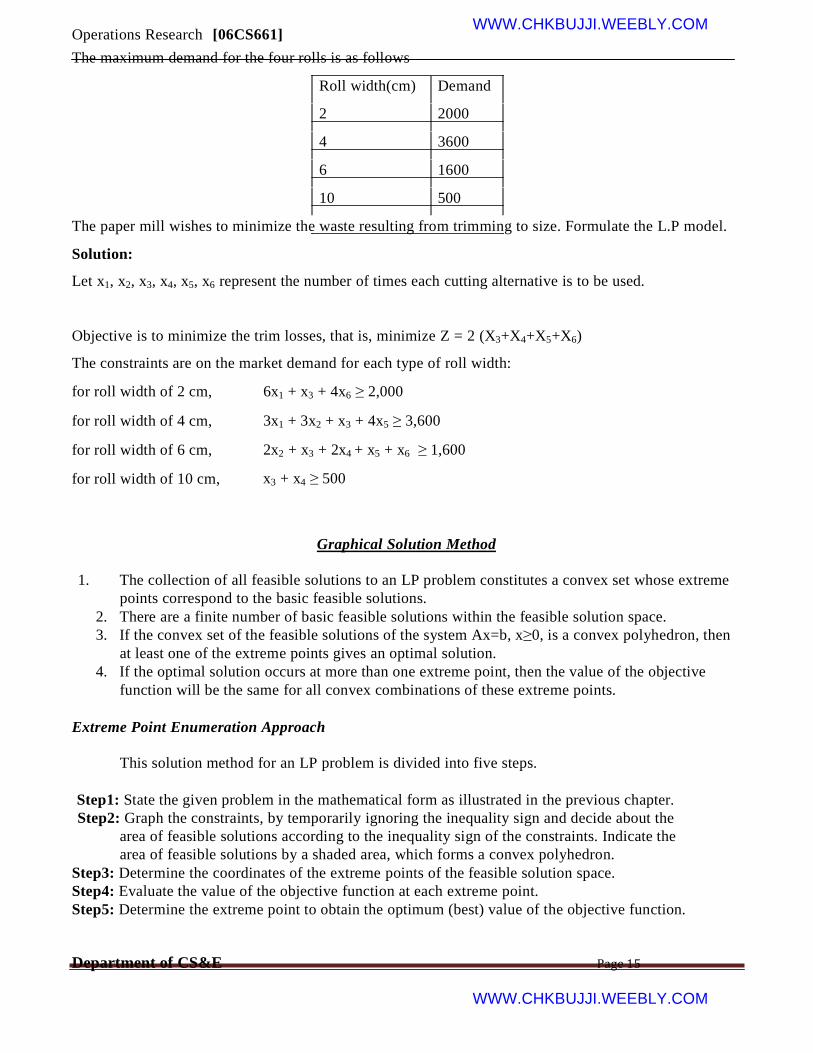
The maximum demand for the four rolls is as follows
Roll width(cm) Demand
2 2000
4 3600
6 1600
10 500
The paper mill wishes to minimize the waste resulting from trimming to size. Formulate the L.P model.
Solution:
Let x1, x2, x3, x4, x5, x6 represent the number of times each cutting alternative is to be used.
Objective is to minimize the trim losses, that is, minimize Z = 2 (X3+X4+X5+X6)
The constraints are on the market demand for each type of roll width:
for roll width of 2 cm,
for roll width of 4 cm,
for roll width of 6 cm,
for roll width of 10 cm,
6x1 + x3 + 4x6 ≥ 2,000
3x1 + 3x2 + x3 + 4x5 ≥ 3,600
2x2 + x3 + 2x4 + x5 + x6 ≥ 1,600
x3 + x4 ≥ 500
Graphical Solution Method
1. The collection of all feasible solutions to an LP problem constitutes a convex set whose extreme
points correspond to the basic feasible solutions.
2. There are a finite number of basic feasible solutions within the feasible solution space.
3. If the convex set of the feasible solutions of the system Ax=b, x≥0, is a convex polyhedron, then
at least one of the extreme points gives an optimal solution.
4. If the optimal solution occurs at more than one extreme point, then the value of the objective
function will be the same for all convex combinations of these extreme points.
Extreme Point Enumeration Approach
This solution method for an LP problem is divided into five steps.
Step1: State the given problem in the mathematical form as illustrated in the previous chapter.
Step2: Graph the constraints, by temporarily ignoring the inequality sign and decide about the
area of feasible solutions according to the inequality sign of the constraints. Indicate the
area of feasible solutions by a shaded area, which forms a convex polyhedron.
Step3: Determine the coordinates of the extreme points of the feasible solution space.
Step4: Evaluate the value of the objective function at each extreme point.
Step5: Determine the extreme point to obtain the optimum (best) value of the objective function.
Department of CS&E Page 15
WWW.CHKBUJJI.WEEBLY.COM
Operations Research [06CS661] WWW.CHKBUJJI.WEEBLY.COM
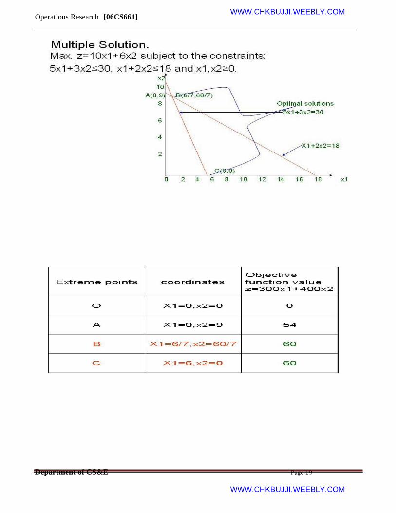
Types of Graphical solutions.
• Single solutions.
• Unique solutions.
• Unbounded solutions.
• Multiple solutions.
• Infeasible solutions.
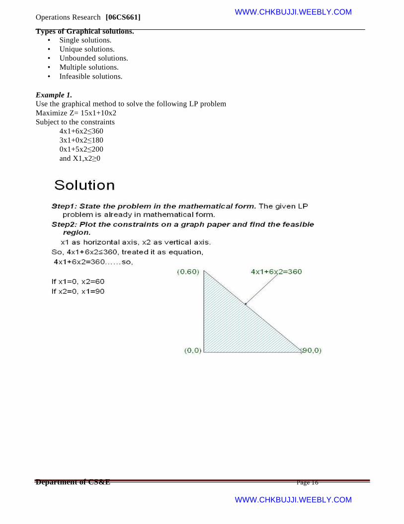
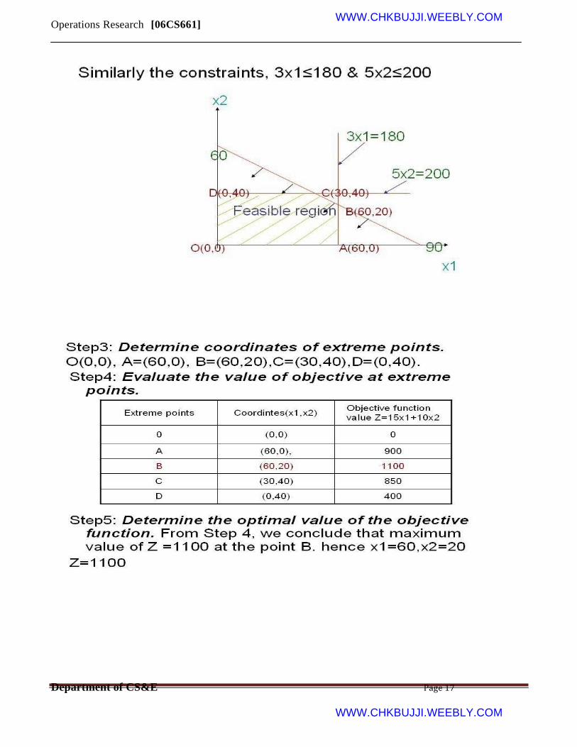
Example 1.
Use the graphical method to solve the following LP problem
Maximize Z= 15x1+10x2
Subject to the constraints
4x1+6x2≤360
3x1+0x2≤180
0x1+5x2≤200
and X1,x2≥0
Department of CS&E Page 16
WWW.CHKBUJJI.WEEBLY.COM
Operations Research [06CS661] WWW.CHKBUJJI.WEEBLY.COM
Department of CS&E Page 17
WWW.CHKBUJJI.WEEBLY.COM

Operations Research [06CS661] WWW.CHKBUJJI.WEEBLY.COM
Department of CS&E Page 18
WWW.CHKBUJJI.WEEBLY.COM
Operations Research [06CS661] WWW.CHKBUJJI.WEEBLY.COM
Department of CS&E Page 19
WWW.CHKBUJJI.WEEBLY.COM
Operations Research [06CS661] WWW.CHKBUJJI.WEEBLY.COM
UNIT-II
Linear Programming Problems
Simplex Method
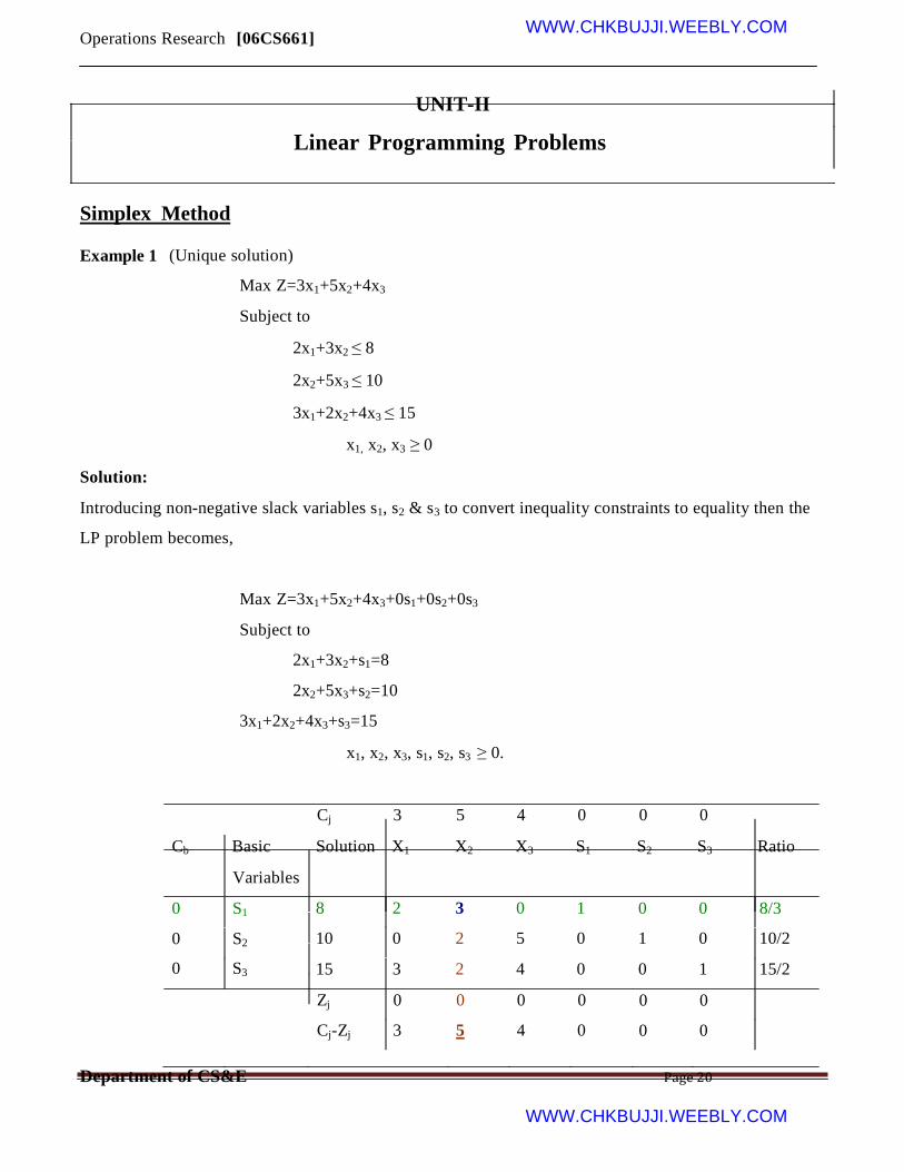
Example 1
Solution:
(Unique solution)
Max Z=3x1+5x2+4x3
Subject to
2x1+3x2 ≤ 8
2x2+5x3 ≤ 10
3x1+2x2+4x3 ≤ 15
x1, x2, x3 ≥ 0
Introducing non-negative slack variables s1, s2 & s3 to convert inequality constraints to equality then the
LP problem becomes,
Max Z=3x1+5x2+4x3+0s1+0s2+0s3
Subject to
2x1+3x2+s1=8
2x2+5x3+s2=10
3x1+2x2+4x3+s3=15
x1, x2, x3, s1, s2, s3 ≥ 0.
Cb Basic
Variables
0 S1
0 S2
0 S3
Cj 3 5 4 0
Solution X1 X2 X3 S1
8 2 3 0 1
10 0 2 5 0
15 3 2 4 0
Zj 0 0 0 0
Cj-Zj 3 5 4 0
0 0
S2 S3 Ratio
0 0 8/3
1 0 10/2
0 1 15/2
0 0
0 0
Department of CS&E Page 20
WWW.CHKBUJJI.WEEBLY.COM

Operations Research [06CS661] WWW.CHKBUJJI.WEEBLY.COM
5 X2 8/3 2/3 1
0 S2 14/3 -4/3 0
0 S3 24/3 5/3 0
Zj 10/3 5
Cj-Zj -1/3 0
5 X2 8/3 2/3 1
4 X3 14/15 -4/15 0
0 S3 89/15 41/15 0
Zj 34/15 5
Cj-Zj 11/15 0
5 X2 50/41 0 1
4 X3 62/41 0 0
3 X1 89/41 1 0
Zj 3 5
Zj-Cj 0 0
0 1/3 0 0 --
5 -2/3 1 0 14/15
4 -2/3 0 1 29/12
0 5/3 0 0
4 -5/3 0 0
0 1/3 0 0 4
1 -2/15 1/5 0 -ve
0 -2/15 -4/5 1 89/41
4 17/15 4/5 0
0 - -4/5 0
17/15
0 15/41 8/41 -
10/41
1 -6/41 5/41 4/41
0 -2/41 - 15/41
12/41
4 45/41 24/41 11/41
0 -ve -ve -ve
All Zj –Cj < 0 for non-basic variable. Therefore the optimal solution is reached.
X1=89/41, X2=50/41, X3=62/41
Z = 3*89/41+5*50/41+4*62/41 = 765/41
Example 2:(unbounded)
Max Z=4x1+x2+3x3+5x4
Subject to
4x1-6x2-5x3-4x4 ≥ -20
-3x1-2x2+4x3+x4 ≤10
-8x1-3x2+3x3+2x4 ≤ 20
x1, x2, x3, x4 ≥ 0.
Solution:
Since the RHS of the first constraints is negative , first it will be made positive by multiplying by
Department of CS&E Page 21
WWW.CHKBUJJI.WEEBLY.COM

Operations Research [06CS661] WWW.CHKBUJJI.WEEBLY.COM –
1, -4x1+6x2+5x3+4x4 ≤ 20
Introducing non-negative slack variable s1, s2 & s3 to convert inequality constraint to equality then the
LP problem becomes.
Max Z=4x1+x2+3x3+5x4+0s1+0s2+0s3
Subject to
-4x1+6x2+5x3+4x4+0s1=20
-3x1-2x1+4x3+x4+s3=10
-8x1-3x2+3x3+2x4+s4=20
x1,x2,x3,x4,s1,s2,s3 ≥ 0
Cj 4 1 3 5 0 0 0
Cb Variables Solution X1 X2 X3 X4 S1 S2 S3 Ratio
0 S1 20 -4
0 S2 10 -3
0 S3 20 -8
Zj 0
CJ-Zj 4
5 X4 5 -1
0 S2 5 -2
0 S3 10 -6
Zj -5
Cj-Zj 9
6 5 4 1 0 0 5
-2 4 1 0 1 0 10
-3 3 2 0 0 1 10
0 0 0 0 0 0
1 3 5 0 0 0
3/2 5/4 1 ¼ 0 0 -ve
-7/2 11/4 0 -1/4 1 0 -ve
-6 ½ 0 -1/2 0 1 -ve
15/2 25/4 5 5/4 0 0
-13/2 -13/4 0 -5/4 0 0
Since all the ratio is negative, the value of incoming non-basic variable x1 can be made as large as we
like without violating condition. Therefore, the problem has an unbounded solution.
Example 3:(infinite solution)
Max Z=4x1+10x2
Subject to
2x1+x2 ≤ 10,
2x1+5x2 ≤ 20,
2x1+3x2 ≤ 18. x1, x2 ≥ 0.
Solution:
Department of CS&E Page 22
WWW.CHKBUJJI.WEEBLY.COM
Operations Research [06CS661] WWW.CHKBUJJI.WEEBLY.COM
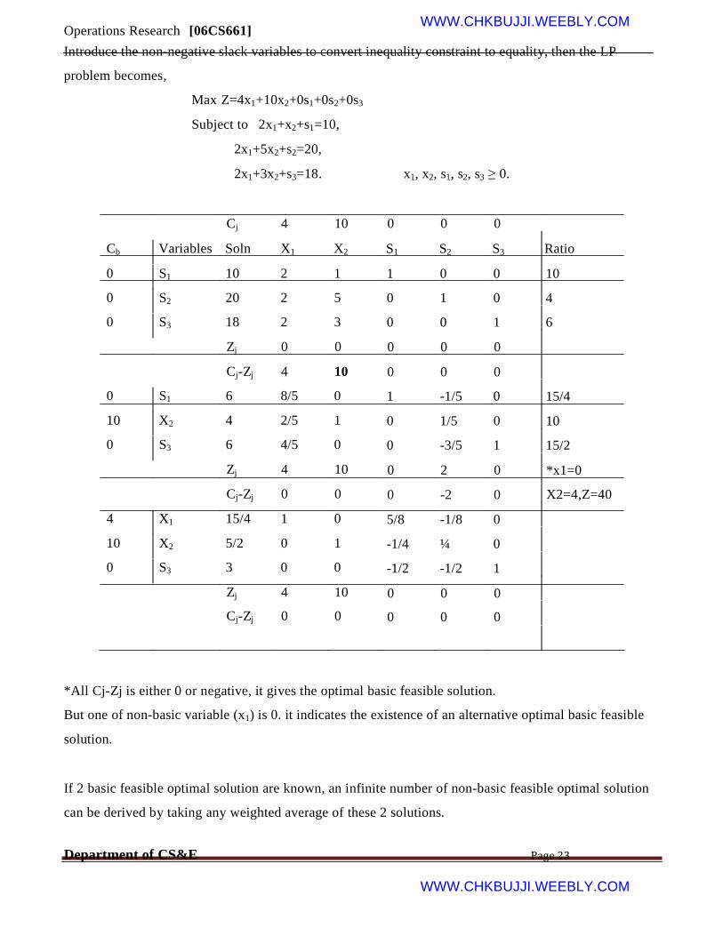
Introduce the non-negative slack variables to convert inequality constraint to equality, then the LP
problem becomes,
Max Z=4x1+10x2+0s1+0s2+0s3
Subject to 2x1+x2+s1=10,
2x1+5x2+s2=20,
2x1+3x2+s3=18. x1, x2, s1, s2, s3 ≥ 0.
Cj 4 10
Cb Variables Soln X1 X2
0 S1 10 2 1
0 S2 20 2 5
0 S3 18 2 3
Zj 0 0
Cj-Zj 4 10
0 S1 6 8/5 0
10 X2 4 2/5 1
0 S3 6 4/5 0
Zj 4 10
Cj-Zj 0 0
4 X1 15/4 1 0
10 X2 5/2 0 1
0 S3 3 0 0
Zj 4 10
Cj-Zj 0 0
0 0 0
S1 S2 S3
1 0 0
0 1 0
0 0 1
0 0 0
0 0 0
1 -1/5 0
0 1/5 0
0 -3/5 1
0 2 0
0 -2 0
5/8 -1/8 0
-1/4 ¼ 0
-1/2 -1/2 1
0 0 0
0 0 0
Ratio
10
4
6
15/4
10
15/2
*x1=0
X2=4,Z=40
*All Cj-Zj is either 0 or negative, it gives the optimal basic feasible solution.
But one of non-basic variable (x1) is 0. it indicates the existence of an alternative optimal basic feasible
solution.
If 2 basic feasible optimal solution are known, an infinite number of non-basic feasible optimal solution
can be derived by taking any weighted average of these 2 solutions.
Department of CS&E Page 23
WWW.CHKBUJJI.WEEBLY.COM
Operations Research [06CS661] WWW.CHKBUJJI.WEEBLY.COM
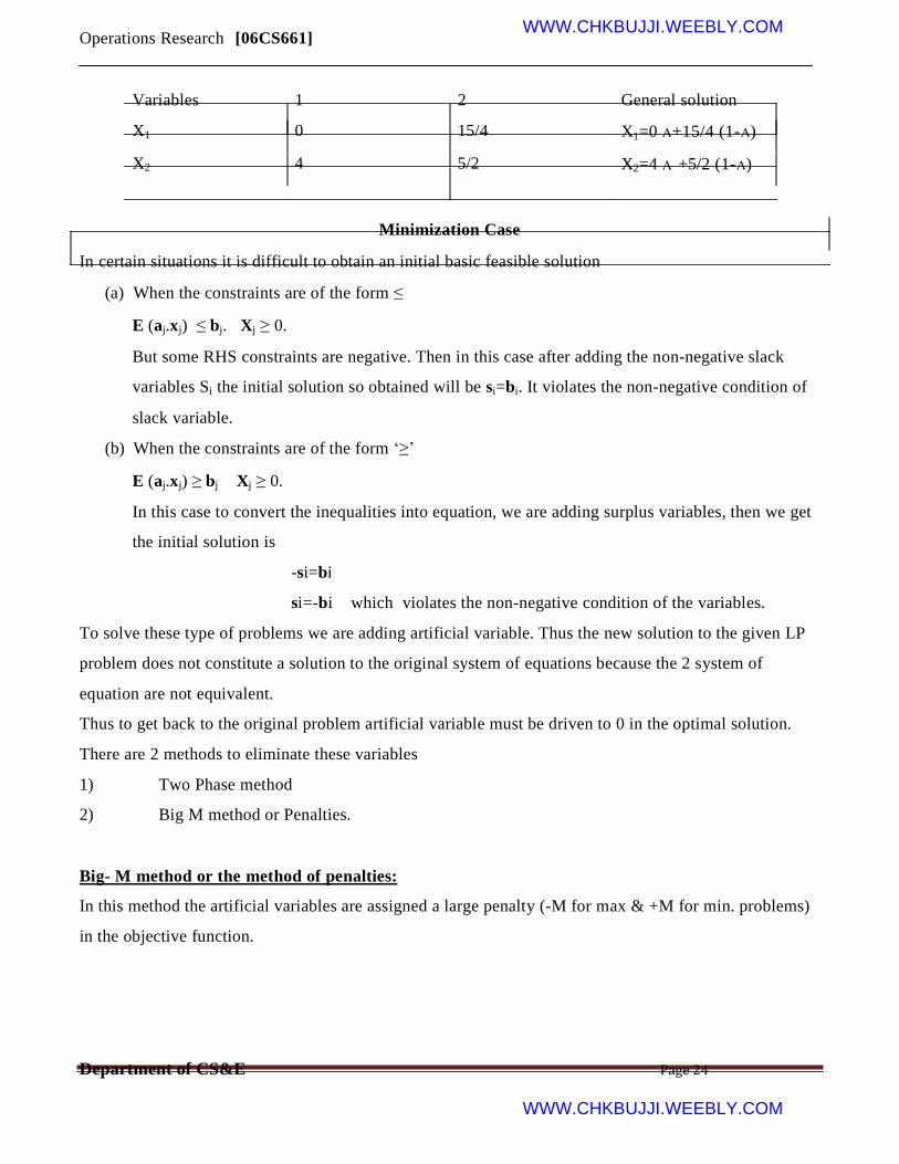
Variables 1
X1 0
X2 4
2 General solution
15/4 X1=0 Α+15/4 (1-Α)
5/2 X2=4 Α +5/2 (1-Α)
Minimization Case
In certain situations it is difficult to obtain an initial basic feasible solution
(a) When the constraints are of the form ≤
E (aj.xj) ≤ bj. Xj ≥ 0.
But some RHS constraints are negative. Then in this case after adding the non-negative slack
variables Si the initial solution so obtained will be si=bi. It violates the non-negative condition of
slack variable.
(b) When the constraints are of the form ‘≥’
E (aj.xj) ≥ bj Xj ≥ 0.
In this case to convert the inequalities into equation, we are adding surplus variables, then we get
the initial solution is
-si=bi
si=-bi which violates the non-negative condition of the variables.
To solve these type of problems we are adding artificial variable. Thus the new solution to the given LP
problem does not constitute a solution to the original system of equations because the 2 system of
equation are not equivalent.
Thus to get back to the original problem artificial variable must be driven to 0 in the optimal solution.
There are 2 methods to eliminate these variables
1) Two Phase method
2) Big M method or Penalties.
Big- M method or the method of penalties:
In this method the artificial variables are assigned a large penalty (-M for max & +M for min. problems)
in the objective function.
Department of CS&E Page 24
WWW.CHKBUJJI.WEEBLY.COM

Operations Research
Example 4:
Solution:
[06CS661]
Max Z =3x1-x2,
Subject to
2x1+x2 ≥ 2
x1+3x2 ≤ 3
x2 ≤ 4
WWW.CHKBUJJI.WEEBLY.COM
x1,x2,x3 ≥ 0
Introduce slack, surplus & artificial variable to convert inequality into equality then the LP problem
becomes
Max Z =3x1-x2+0s1+0s2+0s3+0A1,
Subject to
2x1+x2-s1+A1=2
x1+3x2+s2=3
x2+s3=4 x1,x2,x3,s1,s2,s3,A1 ≥ 0
Cj
Cb Variables Soln
1 A1 2
0 S2 3
0 S3 4
Zj
Cj-Zj
3 X1 1
0 S2 2
0 S3 4
Zj
Cj-Zj
3 X1 3
0 S1 4
0 S3 4
Zj
Cj-Zj
3 -1 0 0 0
X1 X2 S1 S2 S3
2 1 -1 0 0
1 3 0 1 0
0 1 0 0 1
-2M -M M 0 0
3+2M -1+M -M 0 0
1 ½ -1/2 0 0
0 5/2 ½ 1 0
0 1 0 0 1
3 3/2 -3/2 0 0
0 -5/2 3/2 0
1 3 0 1 0
0 5 1 2 0
0 1 0 0 1
3 9 0 3 0
0 -10 0 -3 0
-M
A1 Ratio
1 1
0 3
0 -
-M
0
½ -
-1/2 2
0 -
3/2
-
0
-1
0
0
4
Department of CS&E Page 25
WWW.CHKBUJJI.WEEBLY.COM
Operations Research [06CS661] WWW.CHKBUJJI.WEEBLY.COM
Since the value of Cj-Zj is either negative or 0 under all columns the optimal solution has been obtained.
Therefore x1=3 & x2=0, Z=3x1-x2 =3*3 =9
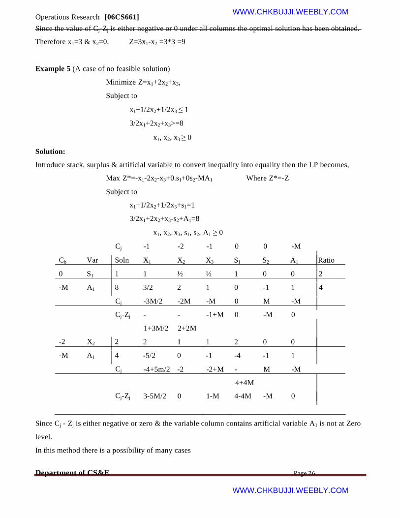
Example 5 (A case of no feasible solution)
Minimize Z=x1+2x2+x3,
Subject to
x1+1/2x2+1/2x3 ≤ 1
3/2x1+2x2+x3>=8
x1, x2, x3 ≥ 0
Solution:
Introduce stack, surplus & artificial variable to convert inequality into equality then the LP becomes,
Max Z*=-x1-2x2-x3+0.s1+0s2-MA1 Where Z*=-Z
Subject to
x1+1/2x2+1/2x3+s1=1
3/2x1+2x2+x3-s2+A1=8
x1, x2, x3, s1, s2, A1 ≥ 0
Cj
Cb Var Soln
0 S1 1
-M A1 8
Cj
Cj-Zj
-2 X2 2
-M A1 4
Cj
Cj-Zj
-1 -2 -1 0 0
X1 X2 X3 S1 S2
1 ½ ½ 1 0
3/2 2 1 0 -1
-3M/2 -2M -M 0 M
- - -1+M 0 -M
1+3M/2 2+2M
2 1 1 2 0
-5/2 0 -1 -4 -1
-4+5m/2 -2 -2+M - M
4+4M
3-5M/2 0 1-M 4-4M -M
-M
A1 Ratio
0 2
1 4
-M
0
0
1
-M
0
Since Cj - Zj is either negative or zero & the variable column contains artificial variable A1 is not at Zero
level.
In this method there is a possibility of many cases
Department of CS&E Page 26
WWW.CHKBUJJI.WEEBLY.COM

Operations Research [06CS661] WWW.CHKBUJJI.WEEBLY.COM
1. Column variable contains no artificial variable. In this case continue the iteration till an optimum
solution is obtained.
2. Column variable contains at least one artificial variable AT Zero level & all Cj-Zj is either
negative or Zero. In this case the current basic feasible solution is optimum through degenerate.
3. Column Variable contains at least one artificial variable not at Zero level. Also Cj - Zj<=0. In this
case the current basic feasible solution is not optimal since the objective function will contain
unknown quantity M, Such a solution is called pseudo-optimum solution.
The Two Phase Method
Phase I:
Step 1: Ensure that all (bi) are non-negative. If some of them are negative, make them non-negative
by multiplying both sides by –1.
Step 2: Express the constraints in standard form.
Step 3: Add non-negative artificial variables.
Step 4: Formulate a new objective function, which consists of the sum of the artificial variables. This
function is called infeasibility function.
Step 5: Using simplex method minimize the new objective function s.t. the constraints of the original
problem & obtain the optimum basic feasible function.
Three cases arise: -
1. Min Z* & at least one artificial variable appears in column variable at positive level. In such a
case, no feasible solution exists for the LPP & procedure is terminated.
2. Min W=0 & at least one artificial variable appears in column variable at Zero level. In such a
case the optimum basic feasible solution to the infeasibility form may or may not be a basic
feasible solution to the given original LPP. To obtain a basic feasible solution continue Phase I &
try to drive all artificial variables out & then continue Phase II.
3. Min W=0 & no artificial variable appears in column variable. In such a case, a basic feasible
solution to the original LPP has been found. Proceed to Phase II.
Phase II:
Use the optimum basic feasible solution of Phase I as a starting solution fir the original LPP. Using
simplex method make iteration till an optimum basic feasible solution for it is obtained.
Note:
The new objective function is always of minimization type regardless of whether the given original
LPP is of max or min type.
Department of CS&E Page 27
WWW.CHKBUJJI.WEEBLY.COM
Operations Research [06CS661] WWW.CHKBUJJI.WEEBLY.COM
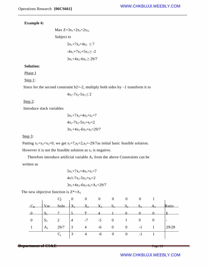
Example 6:
Max Z=3x1+2x2+2x3,
Subject to
5x1+7x2+4x3 ≤ 7
-4x1+7x2+5x3 ≥ -2
3x1+4x2-6x3 ≥ 29/7
Solution:
Phase I
Step 1:
Since for the second constraint b2=-2, multiply both sides by –1 transform it to
4x1-7x2-5x3 ≤ 2
Step 2:
Introduce slack variables
5x1+7x2+4x3+s1=7
4x1-7x2-5x3+s2=2
3x1+4x3-6x3+s3=29/7
Step 3:
Putting x1=x2=x3=0, we get s1=7,s2=2,s3=-29/7as initial basic feasible solution.
However it is not the feasible solution as s1 is negative.
Therefore introduce artificial variable A1 from the above Constraints can be
written as
5x1+7x2+4x3+s1=7
4x1-7x2-5x3+s2=2
3x1+4x2-6x3-s3+A1=29/7
The new objective function is Z*=A1
Cj 0 0 0 0
CB Var Soln X1 X2 X3 S1
0 S1 7 5 7 4 1
0 S2 2 4 -7 -5 0
1 A1 29/7 3 4 -6 0
Cj 3 4 -6 0
0 0 1
S2 S3 A1 Ratio
0 0 0 1
1 0 0 -
0 -1 1 29/28
0 -1 1
Department of CS&E Page 28
WWW.CHKBUJJI.WEEBLY.COM
Operations Research [06CS661] WWW.CHKBUJJI.WEEBLY.COM
Cj-Zj -3 -4
0 X2 1 5/7 1
0 S2 9 9 0
1 A1 1/7 1/7 0
Cj 1/7 0
Cj-Zj -1/7 0
0 X2 2/7 0 1
0 S2 0 0 0
0 X1 1 1 0
Cj 0 0
Cj-Zj 0 0
6 0 0 1 0
4/7 1/7 0 0 0 7/5
-1 1 1 0 0 1
-58/7 -4/7 0 -1 1 1
-58/7 -4/7 0 -1 1
58/7 4/7 0 1 0
294/7 3 0 5 -5
521 37 1 63 -63
-58 -4 0 -7 7
0 0 0 0 0
0 0 0 0 1
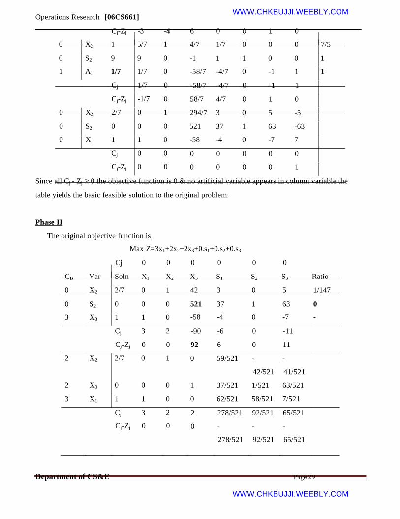
Since all Cj - Zj ≥ 0 the objective function is 0 & no artificial variable appears in column variable the
table yields the basic feasible solution to the original problem.
Phase II
The original objective function is
Max Z=3x1+2x2+2x3+0.s1+0.s2+0.s3
Cj 0 0
CB Var Soln X1 X2
0 X2 2/7 0 1
0 S2 0 0 0
3 X3 1 1 0
Cj 3 2
Cj-Zj 0 0
2 X2 2/7 0 1
2 X3 0 0 0
3 X1 1 1 0
Cj 3 2
Cj-Zj 0 0
0 0
X3 S1
42 3
521 37
-58 -4
-90 -6
92 6
0 59/521
1 37/521
0 62/521
2 278/521
0 -
278/521
0 0
S2 S3 Ratio
0 5 1/147
1 63 0
0 -7 -
0 -11
0 11
- -
42/521 41/521
1/521 63/521
58/521 7/521
92/521 65/521
- -
92/521 65/521
Department of CS&E Page 29
WWW.CHKBUJJI.WEEBLY.COM

Operations Research [06CS661] WWW.CHKBUJJI.WEEBLY.COM
x1=1,x2=2/7,x3=0
z=25/7
Example 7:
(Unconstrained variables)
Min Z=2x1+3x2
Subject to
x1-2x2 ≤0
-2x1+3x2 ≥ -6
x1,x2 unrestricted.
Solution:
The RHS of 2nd constraint id –ve so multiply both sides by –1 we get
2x1-3x2 ≤ 6
as variable x1 & x2 are unrestricted we express them as
x1=y1-y2
x2= y3-y4
where yi ≥ 0 i=1,2,3,4
thus the given problem is transformed to
min Z=2y1-2y2+3y3-3y4
s.t. y1-y2- 2y3+2y4 ≤ 0
-2y1-2y2+ 3y3-3y4 ≤ 6
introduce slack variables we get
Min Z= 2y1-2y2+3y3-3y4+0s1+0s2
Subject to
y1-y2- 2y3+2y4+0s1 ≤0
-2y1-2y2+ 3y3-3y4+0s2 ≤ 6
where all variables are ≥ 0
Cj 2 -2 3 -3 0
CB Var Soln Y1 Y2 Y3 Y4 S1
0 S1 0 1 -1 -2 2 1
0 S2 6 2 -2 -3 3 0
Cj 0 0 0 0 0
0
S2 Ratio
0 0
1 2
0
Department of CS&E Page 30
WWW.CHKBUJJI.WEEBLY.COM

Operations Research [06CS661] WWW.CHKBUJJI.WEEBLY.COM
Cj-Zj 2 -2 3 -3 0 0
-3 Y4 0 ½ -1/2 -1 1 ½ 0 -
0 S2 6 ½ -1/2 0 0 -3/2 1 -
Cj -3/2 3/2 3 -3 3/2 0
Cj-Zj 3/2 -7/2 0 0 -3/2 0
All the ratios are –ve that the value of the incoming non-basic variable y2 can be made as large as
possible without violating the constraint. This problem has unbounded solution & the iteration stops
here.
Note:
If the minimum ratio is equal to for 2 or more rows, arbitrary selection of 1 of these variables may result
in 1 or more variable becoming 0 in the next iteration & the problem is said to degenerate.
These difficulties maybe overcome by applying the following simple procedure called perturbation
method.
1. Divide each element in the tied rows by the positive co-efficient of the key column in that row
2. Compare the resulting ratios, column-by-column 1st in the identity & then in the body from left
to right.
3. The row which first contains the smallest algebraic ratio contains the outgoing variable.
Linear programming - sensitivity analysis
Recall the production planning problem concerned with four variants of the same product which we
formulated before as an LP. To remind you of it we repeat below the problem and our formulation of it.
Production planning problem
A company manufactures four variants of the same product and in the final part of the manufacturing
process there are assembly, polishing and packing operations. For each variant the time required for
these operations is shown below (in minutes) as is the profit per unit sold.
Assembly Variant 1 2
Polish Pack Profit (£) 3 2 1.50
2 4 2 3 2.50
3 3 3 2 3.00
4 7 4 5 4.50
• Given the current state of the labour force the company estimate that, each year, they have
100000 minutes of assembly time, 50000 minutes of polishing time and 60000 minutes of
Department of CS&E Page 31
WWW.CHKBUJJI.WEEBLY.COM

Operations Research [06CS661] WWW.CHKBUJJI.WEEBLY.COM
packing time available. How many of each variant should the company make per year and what
is the associated profit?
• Suppose now that the company is free to decide how much time to devote to each of the three
operations (assembly, polishing and packing) within the total allowable time of 210000 (=
100000 + 50000 + 60000) minutes. How many of each variant should the company make per
year and what is the associated profit?
Production planning solution
Variables
Let: xi be the number of units of variant i (i=1,2,3,4) made per year
Tass be the number of minutes used in assembly per year
Tpol be the number of minutes used in polishing per year
Tpac be the number of minutes used in packing per year
where xi >= 0 i=1,2,3,4 and Tass, Tpol, Tpac >= 0
Constraints
(a) operation time definition
Tass = 2x1 + 4x2 + 3x3 + 7x4 (assembly)
Tpol = 3x1 + 2x2 + 3x3 + 4x4 (polish)
Tpac = 2x1 + 3x2 + 2x3 + 5x4 (pack)
(b) operation time limits
The operation time limits depend upon the situation being considered. In the first situation, where the
maximum time that can be spent on each operation is specified, we simply have:
Tass <= 100000 (assembly)
Tpol <= 50000 (polish)
Tpac <= 60000 (pack)
In the second situation, where the only limitation is on the total time spent on all operations, we simply
have:
Tass + Tpol + Tpac <= 210000 (total time)
Objective
Presumably to maximise profit - hence we have
maximise 1.5x1 + 2.5x2 + 3.0x3 + 4.5x4
which gives us the complete formulation of the problem.
Department of CS&E Page 32
WWW.CHKBUJJI.WEEBLY.COM

Operations Research [06CS661] WWW.CHKBUJJI.WEEBLY.COM
A summary of the input to the computer package for the first situation considered in the question
(maximum time that can be spent on each operation specified) is shown below.
The solution to this problem is also shown below.
We can see that the optimal solution to the LP has value 58000 (£) and that Tass=82000, Tpol=50000,
Tpac=60000, X1=0, X2=16000, X3=6000 and X4=0.
Department of CS&E Page 33
WWW.CHKBUJJI.WEEBLY.COM

Operations Research [06CS661] WWW.CHKBUJJI.WEEBLY.COM
This then is the LP solution - but it turns out that the simplex algorithm (as a by-product of solving the
LP) gives some useful information. This information relates to:
• changing the objective function coefficient for a variable
• forcing a variable which is currently zero to be non-zero
• changing the right-hand side of a constraint.
We deal with each of these in turn, and note here that the analysis presented below ONLY applies for a
single change, if two or more things change then we effectively need to resolve the LP.
• suppose we vary the coefficient of X2 in the objective function. How will the LP optimal solution
change?
Currently X1=0, X2=16000, X3=6000 and X4=0. The Allowable Min/Max c(i) columns above tell us that,
provided the coefficient of X2 in the objective function lies between 2.3571 and 4.50, the values of the
variables in the optimal LP solution will remain unchanged. Note though that the actual optimal solution
value will change.
In terms of the original problem we are effectively saying that the decision to produce 16000 of variant 2
and 6000 of variant 3 remains optimal even if the profit per unit on variant 2 is not actually 2.5 (but lies in
the range 2.3571 to 4.50).
Similar conclusions can be drawn about X1, X3 and X4.
In terms of the underlying simplex algorithm this arises because the current simplex basic solution
(vertex of the feasible region) remains optimal provided the coefficient of X2 in the objective function
lies between 2.3571 and 4.50.
• for the variables, the Reduced Cost column gives us, for each variable which is currently zero
(X1 and X4), an estimate of how much the objective function will change if we make that
variable non-zero.
Hence we have the table
Variable X1 X4
Opportunity Cost 1.5 0.2
New value (= or >=) X1=A X4=B
or X1>=A X4>=B
Estimated objective function change 1.5A 0.2B
The objective function will always get worse (go down if we have a maximisation problem, go up if we
have a minimisation problem) by at least this estimate. The larger A or B are the more inaccurate this
estimate is of the exact change that would occur if we were to resolve the LP with the corresponding
constraint for the new value of X1 or X4 added.
Hence if exactly 100 of variant one were to be produced what would be your estimate of the new
objective function value?
Department of CS&E Page 34
WWW.CHKBUJJI.WEEBLY.COM

Operations Research [06CS661] WWW.CHKBUJJI.WEEBLY.COM
Note here that the value in the Reduced Cost column for a variable is often called the "opportunity cost"
for the variable.
Note here than an alternative (and equally valid) interpretation of the reduced cost is the amount
by which the objective function coefficient for a variable needs to change before that variable will
become non-zero.
Hence for variable X1 the objective function needs to change by 1.5 (increase since we are maximising)
before that variable becomes non-zero. In other words, referring back to our original situation, the profit
per unit on variant 1 would need to need to increase by 1.5 before it would be profitable to produce any
of variant 1. Similarly the profit per unit on variant 4 would need to increase by 0.2 before it would be
profitable to produce any of variant 4.
• for each constraint the column headed Shadow Price tells us exactly how much the objective
function will change if we change the right-hand side of the corresponding constraint within the
limits given in the Allowable Min/Max RHS column.
Hence we can form the table
Constraint Assembly Polish Pack
Opportunity Cost (ignore sign) 0
Change in right-hand side a
0.80 0.30
b c
Objective function change 0 0.80b 0.30c
Lower limit for right-hand side 82000 Current value for right-hand side 100000
40000 33333.34 50000 60000
Upper limit for right-hand side - 90000 75000
For example for the polish constraint, provided the right-hand side of that constraint remains between
40000 and 90000 the objective function change will be exactly 0.80[change in right-hand side from
50000].
The direction of the change in the objective function (up or down) depends upon the direction of the
change in the right-hand side of the constraint and the nature of the objective (maximise or minimise).
To decide whether the objective function will go up or down use:
• constraint more (less) restrictive after change in right-hand side implies objective function worse
(better)
• if objective is maximise (minimise) then worse means down (up), better means up (down)
Hence
• if you had an extra 100 hours to which operation would you assign it?
• if you had to take 50 hours away from polishing or packing which one would you choose?
• what would the new objective function value be in these two cases?
The value in the column headed Shadow Price for a constraint is often called the "marginal value" or
"dual value" for that constraint.
Department of CS&E Page 35
WWW.CHKBUJJI.WEEBLY.COM
Operations Research [06CS661] WWW.CHKBUJJI.WEEBLY.COM
Note that, as would seem logical, if the constraint is loose the shadow price is zero (as if the constraint is
loose a small change in the right-hand side cannot alter the optimal solution).
Comments
• Different LP packages have different formats for input/output but the same information as
discussed above is still obtained.
• You may have found the above confusing. Essentially the interpretation of LP output is
something that comes with practice.
• Much of the information obtainable (as discussed above) as a by-product of the solution of the
LP problem can be useful to management in estimating the effect of changes (e.g. changes in
costs, production capacities, etc) without going to the hassle/expense of resolving the LP.
• This sensitivity information gives us a measure of how robust the solution is i.e. how sensitive it
is to changes in input data.
Note here that, as mentioned above, the analysis given above relating to:
• changing the objective function coefficient for a variable; and
• forcing a variable which is currently zero to be non-zero; and
• changing the right-hand side of a constraint
is only valid for a single change. If two (or more) changes are made the situation becomes more
complex and it becomes advisable to resolve the LP.
Linear programming sensitivity example
Consider the linear program:
maximise
3x1 + 7x2 + 4x3 + 9x4
subject to
x1 + 4x2 + 5x3 + 8x4 <= 9 (1)
x1 + 2x2 + 6x3 + 4x4 <= 7 (2)
xi >= 0 i=1,2,3,4
Solve this linear program using the computer package.
• what are the values of the variables in the optimal solution?
• what is the optimal objective function value?
• which constraints are tight?
• what would you estimate the objective function would change to if:
o we change the right-hand side of constraint (1) to 10
o we change the right-hand side of constraint (2) to 6.5
o we add to the linear program the constraint x3 = 0.7
Solving the problem using the package the solution is:
Department of CS&E Page 36
WWW.CHKBUJJI.WEEBLY.COM

Operations Research [06CS661] WWW.CHKBUJJI.WEEBLY.COM
Reading from the printout given above we have:
• the variable values are X1=5, X2=1, X3=0, X4=0
• the optimal objective function value is 22.0
• both constraints are tight (have no slack or surplus). Note here that the (implicit) constraints
ensuring that the variables are non-negative (xi>=0 i=1,2,3,4) are (by convention) not considered
in deciding which constraints are tight.
• objective function change = (10-9) x 0.5 = 0.5. Since the constraint is less restrictive the
objective function will get better. Hence as we have a maximisation problem it will increase.
Referring to the Allowable Min/Max RHS column we see that the new value (10) of the right-
hand side of constraint (1) is within the limits specified there so that the new value of the
objective function will be exactly 22.0 + 0.5 = 22.5
• objective function change = (7-6.5) x 2.5 = 1.25. Since we are making the constraint more
restrictive the objective function will get worse. Hence as we have a maximisation problem it will
decrease. As for (1) above the new value of the right-hand side of constraint (2) is within the
limits in the Minimum/Maximum RHS column and so the new value of the objective function will
be exactly 22.0 - 1.25 = 20.75
• objective function change = 0.7 x 13.5 = 9.45. The objective function will get worse (decrease)
since changing any variable which is zero at the linear programming optimum to a non-zero value
always makes the objective function worse. We estimate that it will decrease to 22.0 - 9.45 =
12.55. Note that the value calculated here is only an estimate of the change in the objective
function value. The actual change may be different from the estimate (but will always be >= this
estimate).
Note that we can, if we wish, explicitly enter the four constraints xi>=0 i=1,2,3,4. Although this is
unnecessary (since the package automatically assumes that each variable is >=0) it is not incorrect.
However, it may alter some of the solution figures - in particular the Reduced Cost figures may be
different. This illustrates that such figures are not necessarily uniquely defined at the linear
programming optimal solution.
Department of CS&E Page 37
WWW.CHKBUJJI.WEEBLY.COM
Operations Research [06CS661] WWW.CHKBUJJI.WEEBLY.COM
UNIT-III
Transportation Model
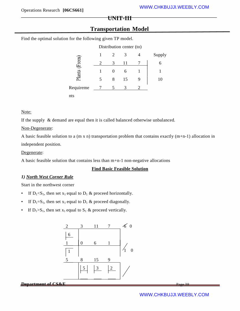
Find the optimal solution for the following given TP model.
Distribution center (to)
1 2 3 4 Supply
2 3 11 7 6
1 0 6 1 1
5 8 15 9 10
Requireme 7 5 3 2
nts
Note:
If the supply & demand are equal then it is called balanced otherwise unbalanced.
Non-Degenerate:
A basic feasible solution to a (m x n) transportation problem that contains exactly (m+n-1) allocation in
independent position.
Degenerate:
A basic feasible solution that contains less than m+n-1 non-negative allocations
Find Basic Feasible Solution
1) North West Corner Rule
Start in the northwest corner
• If D1<S1, then set x1 equal to D1 & proceed horizontally.
• If D1=S1, then set x1 equal to D1 & proceed diagonally.
• If D1>S1, then set x1 equal to S1 & proceed vertically.
2 3 11 7 6 0
6
1 0 6 1
1 1 0
5 8 15 9
5 3 2
Department of CS&E Page 38
WWW.CHKBUJJI.WEEBLY.COM

Operations Research [06CS661] WWW.CHKBUJJI.WEEBLY.COM
10 5 3 2
7 5 3 2
6 0 0 0
1
it can be easily seen that the proposed solution is a feasible solution since all the supply & requirement
constraints are fully satisfied. In this method, allocations have been made without any consideration of
cost of transformation associated with them.
Hence the solution obtained may not be feasible or the best solution.
The transport cost associate with this solution is :
Z=Rs (2*6+1*1+8*5+15*3+9*2) * 100
=Rs (12+1+40+45+18) * 100
=Rs 11600
2) Row Minima Method
This method consists in allocating as much as possible in the lowest cost cell of the 1st row so that either
the capacity of the 1st plant is exhausted or the requirement at the jth distribution center is satisfied or both
Three cases arises:
• If the capacity of the 1st plant is completely exhausted, cross off the 1st row & proceed to the 2nd row.
• If the requirement of the jth distribution center is satisfied, cross off the jth column & reconsider the
1st row with the remaining capacity.
• If the capacity of the 1st plant as well as the requirement at jth distribution center are completely
satisfied, make a 0 allocation in the 2nd lowest cost cell of the 1st row. Cross of the row as well as the
jth column & move down to the 2nd row.
2 3 11 7
6 6 0
1 0 6 1
1 1 0
5 8 15 9
1 4 3 2
10 9 5 3 0
7 5 3 2
Department of CS&E Page 39
WWW.CHKBUJJI.WEEBLY.COM

Operations Research [06CS661]
1 0 0
0
WWW.CHKBUJJI.WEEBLY.COM 0
Z=100 * (6*2+0*1+5*1+8*4+15*3+9*2)
=100 * (12+0+5+32+45+18) =100 * 112 =11200
3) Column Minima Method
2 3 11 7
6 6
0 1 0 6 1
1 1 0
5 8 15 9
5 3 2
10 5 3 2 0
7 5 3 2
6 0 0 0
1
0
Z= 2*6+1*1+5*0+5*8+15+18
= 12+1+40+45+18
= 116
4) Least Cost Method
This method consists of allocating as much as possible in the lowest cost cell/cells& then further
allocation is done in the cell with the 2nd lowest cost.
Department of CS&E Page 40
WWW.CHKBUJJI.WEEBLY.COM
Operations Research [06CS661] WWW.CHKBUJJI.WEEBLY.COM 2
3 11 7
6 6 0
1 0 6 1
1
5 8 15 9 1 0
1 4 3 2
10 9 5 2 0
7 5 3 2
1 4 0 0
0 0
Z= 12+0+5+32+45+18
= 112
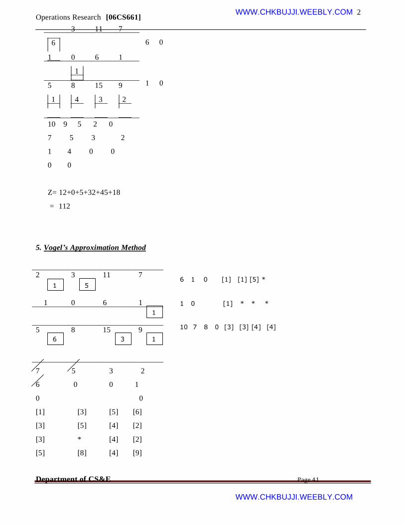
5. Vogel’s Approximation Method
2 3 11 7
1 5
6 1 0 [1] [1] [5] *
1 0 6 1 1 0 [1] * * *
1
5 8 15 9 10 7 8 0 [3] [3] [4] [4]
6 3 1
7 5 3 2
6 0 0 1
0 0
[1] [3] [5] [6]
[3] [5] [4] [2]
[3] * [4] [2]
[5] [8] [4] [9]
Department of CS&E Page 41
WWW.CHKBUJJI.WEEBLY.COM
Operations Research [06CS661] WWW.CHKBUJJI.WEEBLY.COM z
= 2 + 15 + 1 + 30 + 45 + 9
= 102
Perform Optimality Test
An optimality test can, of course, be performed only on that feasible solution in which:
(a) Number of allocations is m+n-1
(b) These m+n-1 allocations should be in independent positions.
A simple rule for allocations to be in independent positions is that it is impossible to travel from any
allocation, back to itself by a series of horizontal & vertical jumps from one occupied cell to another,
without a direct reversal of route.
Now test procedure for optimality involves the examination of each vacant cell to find whether or not
making an allocation in it reduces the total transportation cost.
The 2 methods usually used are:
(1) Stepping-Stone method
(2) The modified distribution (MODI) method
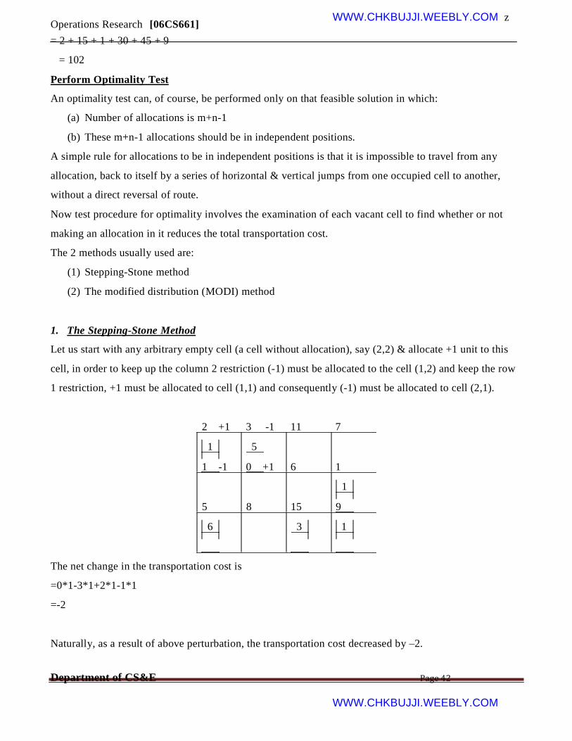
1. The Stepping-Stone Method
Let us start with any arbitrary empty cell (a cell without allocation), say (2,2) & allocate +1 unit to this
cell, in order to keep up the column 2 restriction (-1) must be allocated to the cell (1,2) and keep the row
1 restriction, +1 must be allocated to cell (1,1) and consequently (-1) must be allocated to cell (2,1).
2 +1 3 -1 11 7
1 5
1 -1 0 +1 6 1
1
5 8 15 9
6 3 1
The net change in the transportation cost is
=0*1-3*1+2*1-1*1
=-2
Naturally, as a result of above perturbation, the transportation cost decreased by –2.
Department of CS&E Page 42
WWW.CHKBUJJI.WEEBLY.COM
Operations Research [06CS661] WWW.CHKBUJJI.WEEBLY.COM
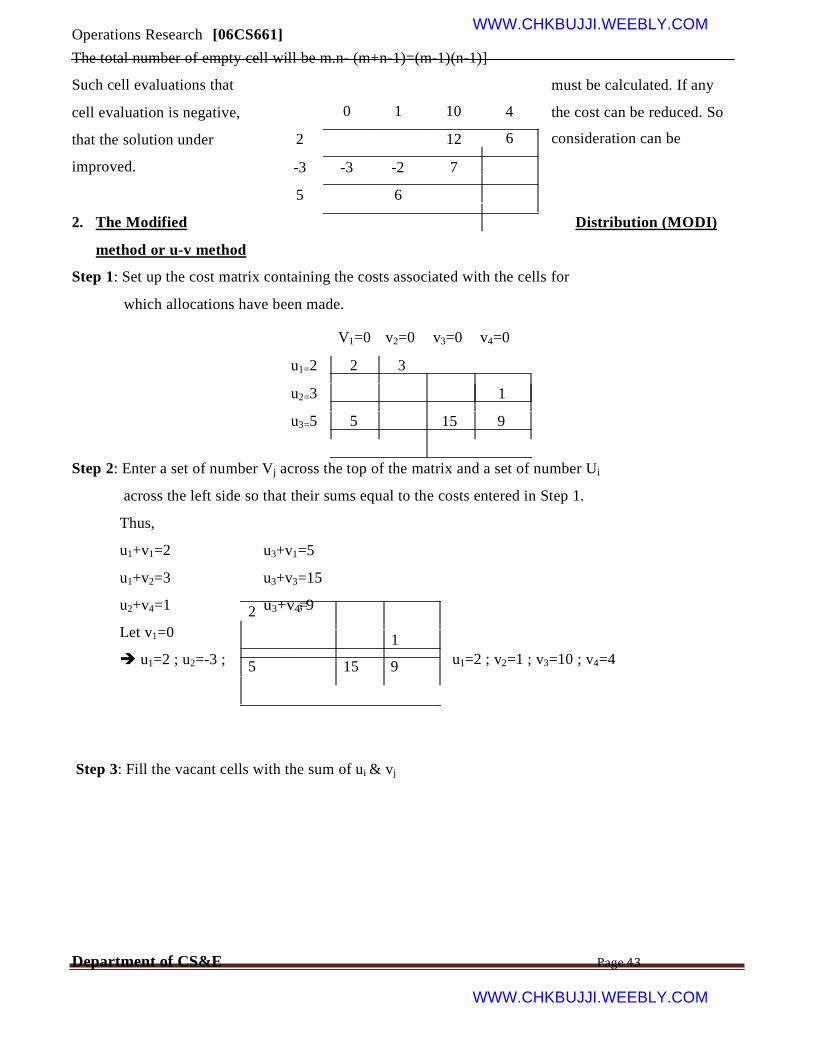
The total number of empty cell will be m.n- (m+n-1)=(m-1)(n-1)]
Such cell evaluations that
cell evaluation is negative,
that the solution under
improved.
0 1 10
2 12
-3 -3 -2 7
5 6
must be calculated. If any
4 the cost can be reduced. So
6 consideration can be
2. The Modified Distribution (MODI)
method or u-v method
Step 1: Set up the cost matrix containing the costs associated with the cells for
which allocations have been made.
V1=0 v2=0
u1=2 2 3
u2=3
u3=5 5
v3=0 v4=0
1
15 9
Step 2: Enter a set of number Vj across the top of the matrix and a set of number Ui
across the left side so that their sums equal to the costs entered in Step 1.
Thus,
u1+v1=2
u1+v2=3
u2+v4=1
Let v1=0
u1=2 ; u2=-3 ;
u3+v1=5
u3+v3=15
2 u3+v4=9
1
5 15 9 u1=2 ; v2=1 ; v3=10 ; v4=4
Step 3: Fill the vacant cells with the sum of ui & vj
Department of CS&E Page 43
WWW.CHKBUJJI.WEEBLY.COM
Operations Research [06CS661] WWW.CHKBUJJI.WEEBLY.COM
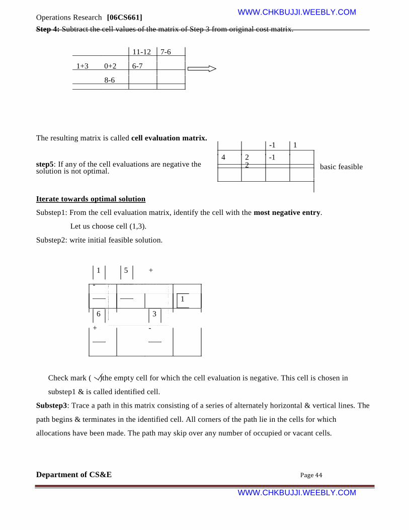
Step 4: Subtract the cell values of the matrix of Step 3 from original cost matrix.
11-12 7-6
1+3 0+2 6-7
8-6
The resulting matrix is called cell evaluation matrix. -1 1
4 2 -1 step5: If any of the cell evaluations are negative the solution is not optimal.
2
basic feasible
Iterate towards optimal solution
Substep1: From the cell evaluation matrix, identify the cell with the most negative entry.
Let us choose cell (1,3).
Substep2: write initial feasible solution.
1 5 +
-
1
6 3
+ -
Check mark ( )the empty cell for which the cell evaluation is negative. This cell is chosen in
substep1 & is called identified cell.
Substep3: Trace a path in this matrix consisting of a series of alternately horizontal & vertical lines. The
path begins & terminates in the identified cell. All corners of the path lie in the cells for which
allocations have been made. The path may skip over any number of occupied or vacant cells.
Department of CS&E Page 44
WWW.CHKBUJJI.WEEBLY.COM

Operations Research [06CS661] WWW.CHKBUJJI.WEEBLY.COM
Substep4: Mark the identified cells as positive and each occupied cell at the corners of the path
alternatively negative & positive & so on.
Note :In order to maintain feasibility locate the occupied cell with minus sign that has the smallest
allocation
Substep5: Make a new allocation in the identified cell.
1-1=0 5 1
1
7 2 1
2 3 11 7
5 1
1 0 6 1 1
5 8 15 5 7 2 1
The total cost of transportation for this 2nd feasible solution is
=Rs (3*5+11*1+1*1+7*5+2*15+1*9)
=Rs (15+11+1+35+30+9)
=Rs 101
Check for optimality
In the above feasible solution
a) number of allocations is (m+n-1) is 6
b) these (m+ n – 1)allocation are independent positions.
Above conditions being satisfied, an optimality test can be performed.
MODI method
Step1: Write down the cost matrix for which allocations have been made.
Step2: Enter a set of number Vj across the top of the matrix and a set of number Ui across the left side so
that their sums equal to the costs entered in Step1.
Thus,
u1+v2=3 u3+v1=5
Department of CS&E Page 45
WWW.CHKBUJJI.WEEBLY.COM

Operations Research [06CS661] WWW.CHKBUJJI.WEEBLY.COM
u1+v3=11
u2+v4=1
Let v1=0
u3+v3=15
u3+v4=9
u1=1 ; u2=-3 ; u3=5 ; v2=2 ; v3=10 ; v4=4
v1 v2 v3 v4
u1 3 11
u2 1
u3 5 15 9
Step3: Fill the vacant cells with the sums of vj & ui
v1=0 v2=2
U1=1 1
U2=-3 -3 -1
U3=5 7
v3=10 v4=4
5
7
Step4: Subtract from the original matrix.
2-1 7-5 1 2
1+3 0+1 6-7 4 1 -1
8-7 -1
Step5: Since one cell is negative, 2nd feasible solution is not optimal.
Iterate towards an optimal solution
Substep1: Identify the cell with most negative entry. It is the cell (2,3).
Substep2: Write down the feasible solution.
5 1
+ 1 -
7 2 - 1 +
Substep3: Trace the path.
Substep4: Mark the identified cell as positive & others as negative alternatively.
Substep5:
5 1
Third feasible solutions
Department of CS&E Page 46
WWW.CHKBUJJI.WEEBLY.COM

Operations Research
7
[06CS661] WWW.CHKBUJJI.WEEBLY.COM 1
1 2
Z=(5*3+1*11+1*6+1*15+2*9+7*5)
=100
Test for optimality
In the above feasible solutions
a)
b)
Step1: setup cost matrix
number of allocation is (m+n-1) that is, 6
these (m+n-1) are independent.
3 11
6
5 15 9
Step2: Enter a set of number Vj across the top of the matrix and a set of number Ui across the left side so
that their sums equal to the costs entered in Step1.
Thus,
u1+v2=3
u1+v3=11
u2+v3=6
u3+v1=5
u3+v3=15
u3+v4=9
let v1 = 0, u3 =5 u2=-4, u1=1, v2=2, v3=10, v4=4
the resulting matrix is
0 2 10 4
1 1 5
-4 -4 -2 0
5 7
Subtract from original cost matrix, we will get cell evaluation matrix
1 2
5 2 1
Department of CS&E Page 47
WWW.CHKBUJJI.WEEBLY.COM

Operations Research [06CS661] WWW.CHKBUJJI.WEEBLY.COM 1
Since all the cells are positive, the third feasible solution is optimal solution.
Assignment Problem
Step 1: Prepare a square matrix: Since the solution involves a square matrix, this step is not necessary.
Step 2: Reduce the matrix: This involves the following substeps.
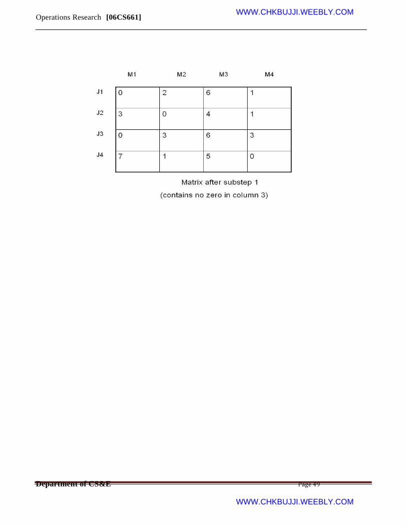
Substep 1: In the effectiveness matrix, subtract the minimum element of each row from all the
elements of the row. See if there is atleast one zero in each row and in each column. If it is so, stop here.
If it is so, stop here. If not proceed to substep 2.
Department of CS&E Page 48
WWW.CHKBUJJI.WEEBLY.COM
Operations Research [06CS661] WWW.CHKBUJJI.WEEBLY.COM
Department of CS&E Page 49
WWW.CHKBUJJI.WEEBLY.COM

Operations Research [06CS661] WWW.CHKBUJJI.WEEBLY.COM
SUBSTEP 2: Next examine columns for single unmarked zeroes and mark them suitably.
SUBSTEP 3: In the present example, after following substeps 1 and 2 we find that their repetition is
unnecessary and also row 3 and column 3 are without any assignments. Hence we proceed as follows to
find the minimum number of lines crossing all zeroes.
SUBSTEP 4: Mark the rows for which assignment has not been made. In our problem it is the third row.
SUBSTEP 5: Mark columns (not already marked) which have zeroes in marked rows. Thus column 1 is
marked.
SUBSTEP 6: Mark rows(not already marked) which have assignmentsin marked columns. Thus row 1 is
marked.
Department of CS&E Page 50
WWW.CHKBUJJI.WEEBLY.COM
Operations Research [06CS661] WWW.CHKBUJJI.WEEBLY.COM
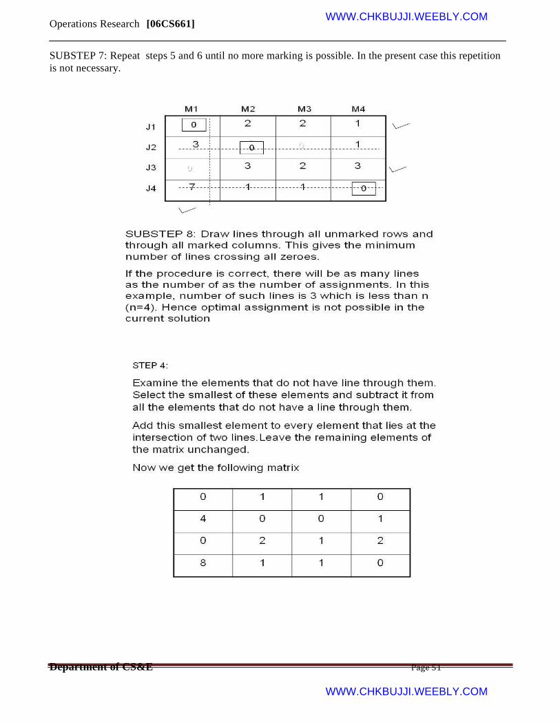
SUBSTEP 7: Repeat steps 5 and 6 until no more marking is possible. In the present case this repetition
is not necessary.
Department of CS&E Page 51
WWW.CHKBUJJI.WEEBLY.COM

Operations Research [06CS661] WWW.CHKBUJJI.WEEBLY.COM
Department of CS&E Page 52
WWW.CHKBUJJI.WEEBLY.COM

Operations Research [06CS661] WWW.CHKBUJJI.WEEBLY.COM
Department of CS&E Page 53
WWW.CHKBUJJI.WEEBLY.COM

Operations Research [06CS661] WWW.CHKBUJJI.WEEBLY.COM
Department of CS&E Page 54
WWW.CHKBUJJI.WEEBLY.COM

Operations Research [06CS661] WWW.CHKBUJJI.WEEBLY.COM
Cost = 61
THE TRAVELLING SALESMAN PROBLEM
The condition for TSP is that no city is visited twice before the tour of all the cities is completed.
A B C D E
A 0 2 5 7 1
B 6 0 3 8 2
C 8 7 0 4 7
D 12 4 6 0 5
E 1 3 2 8 0
As going from A->A,B->B etc is not allowed, assign a large penalty to these cells in the cost matrix
Department of CS&E Page 55
WWW.CHKBUJJI.WEEBLY.COM

Operations Research [06CS661] WWW.CHKBUJJI.WEEBLY.COM
A B C D E A
� 1
4
6
0
A
B
4 � 1
6
0
B
C
4
3 � 0
3
C
D
8
0
2 � 1
D
E
0
2
1
7 � E
A B C D E
� 1
3
6
0
4 �
0
6 0
4
3 �
0
3 8
0
1 �
1
0
2
0
7 �
A B C D E
A � 1 3 6
B 4 � 0 6 0
0
C 4 3 � 0 3
D 8 1 � 1
E 0 2 0 7 �
0
Which gives optimal for assignment problem but not for TSP because the path A->E, E-A, B->C->D->B
does not satisfy the additional constraint of TSP
The next minimum element is 1, so we shall try to bring element 1 into the solution. We have three
cases.
Case 1:
Make assignment in cell (A,B) instead of (A,E).
A B C D E
A ∞ 1 3 6 0
B 4 ∞ 0 6 0
C 4 3 ∞ 3 0
D 8 0 1 ∞ 1
E 0 2 0 7 ∞
The resulting feasible solution is A->B,B-C, C->D,D->E,E->A and cost is 15
Now make assignment in cell (D,C) instead of (D,B)
Department of CS&E Page 56
WWW.CHKBUJJI.WEEBLY.COM
Operations Research [06CS661] WWW.CHKBUJJI.WEEBLY.COM
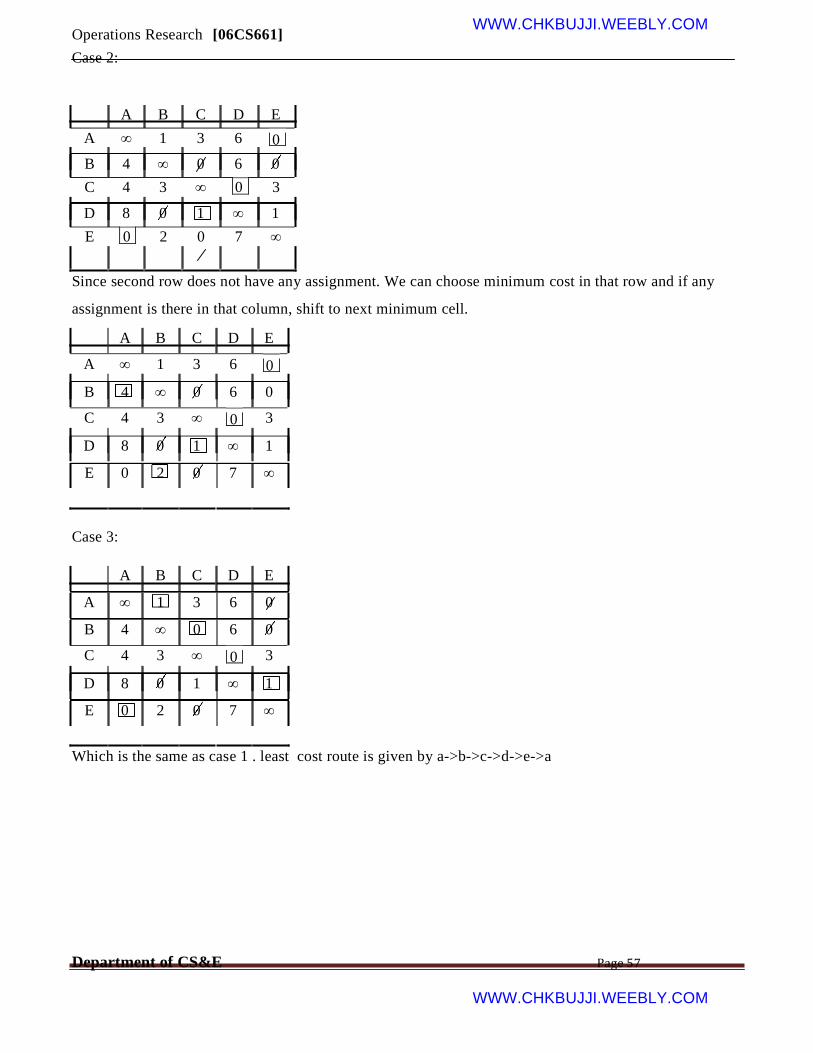
Case 2:
A B C D E
A ∞ 1 3 6 0
B 4 ∞ 0 6 0
C 4 3 ∞ 0 3
D 8 0 1 ∞ 1
E 0 2 0 7 ∞
Since second row does not have any assignment. We can choose minimum cost in that row and if any
assignment is there in that column, shift to next minimum cell.
A B C D E
A ∞ 1 3 6 0
B 4 ∞ 0 6 0
C 4 3 ∞ 3 0
D 8 0 1 ∞ 1
E 0 2 0 7 ∞
Case 3:
A B C D E
A ∞ 1 3 6 0
B 4 ∞ 0 6 0
C 4 3 ∞ 3 0
D 8 0 1 ∞ 1
E 0 2 0 7 ∞
Which is the same as case 1 . least cost route is given by a->b->c->d->e->a
Department of CS&E Page 57
WWW.CHKBUJJI.WEEBLY.COM
Operations Research [06CS661] WWW.CHKBUJJI.WEEBLY.COM
UNIT-V
Queuing theory
Queuing theory deals with problems which involve queuing (or waiting). Typical examples might be:
• banks/supermarkets - waiting for service
• computers - waiting for a response
• failure situations - waiting for a failure to occur e.g. in a piece of machinery
• public transport - waiting for a train or a bus
As we know queues are a common every-day experience. Queues form because resources are limited. In
fact it makes economic sense to have queues. For example how many supermarket tills you would need to
avoid queuing? How many buses or trains would be needed if queues were to be avoided/eliminated?
In designing queueing systems we need to aim for a balance between service to customers (short queues
implying many servers) and economic considerations (not too many servers).
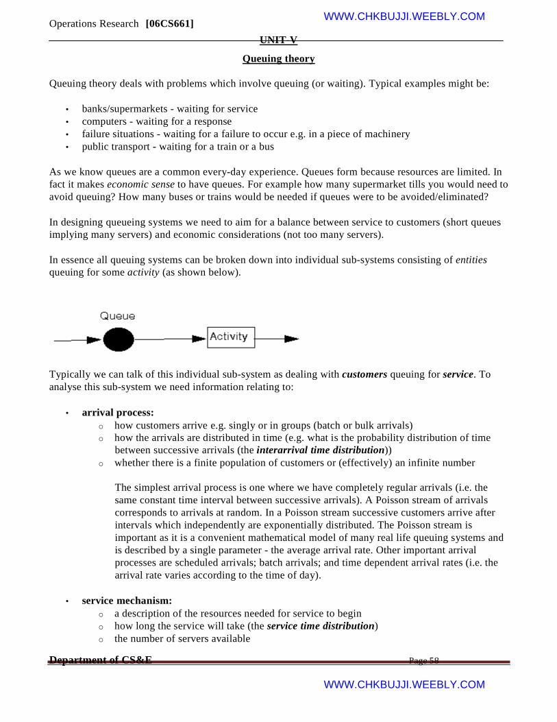
In essence all queuing systems can be broken down into individual sub-systems consisting of entities
queuing for some activity (as shown below).
Typically we can talk of this individual sub-system as dealing with customers queuing for service. To
analyse this sub-system we need information relating to:
• arrival process:
o how customers arrive e.g. singly or in groups (batch or bulk arrivals)
o how the arrivals are distributed in time (e.g. what is the probability distribution of time
between successive arrivals (the interarrival time distribution))
o whether there is a finite population of customers or (effectively) an infinite number
The simplest arrival process is one where we have completely regular arrivals (i.e. the
same constant time interval between successive arrivals). A Poisson stream of arrivals
corresponds to arrivals at random. In a Poisson stream successive customers arrive after
intervals which independently are exponentially distributed. The Poisson stream is
important as it is a convenient mathematical model of many real life queuing systems and
is described by a single parameter - the average arrival rate. Other important arrival
processes are scheduled arrivals; batch arrivals; and time dependent arrival rates (i.e. the
arrival rate varies according to the time of day).
• service mechanism:
o a description of the resources needed for service to begin
o how long the service will take (the service time distribution)
o the number of servers available
Department of CS&E Page 58
WWW.CHKBUJJI.WEEBLY.COM
Operations Research [06CS661] WWW.CHKBUJJI.WEEBLY.COM
o whether the servers are in series (each server has a separate queue) or in parallel (one
queue for all servers)
o whether preemption is allowed (a server can stop processing a customer to deal with
another "emergency" customer)
Assuming that the service times for customers are independent and do not depend upon
the arrival process is common. Another common assumption about service times is that
they are exponentially distributed.
• queue characteristics:
o how, from the set of customers waiting for service, do we choose the one to be served
next (e.g. FIFO (first-in first-out) - also known as FCFS (first-come first served); LIFO
(last-in first-out); randomly) (this is often called the queue discipline)
o do we have: balking (customers deciding not to join the queue if it is too long)
reneging (customers leave the queue if they have waited too long for service)
jockeying (customers switch between queues if they think they will get served
faster by so doing)
a queue of finite capacity or (effectively) of infinite capacity
Changing the queue discipline (the rule by which we select the next customer to be
served) can often reduce congestion. Often the queue discipline "choose the customer
with the lowest service time" results in the smallest value for the time (on average) a
customer spends queuing.
Note here that integral to queuing situations is the idea of uncertainty in, for example, interarrival times
and service times. This means that probability and statistics are needed to analyse queuing situations.
In terms of the analysis of queuing situations the types of questions in which we are interested are
typically concerned with measures of system performance and might include:
• How long does a customer expect to wait in the queue before they are served, and how long will
they have to wait before the service is complete?
• What is the probability of a customer having to wait longer than a given time interval before they
are served?
• What is the average length of the queue?
• What is the probability that the queue will exceed a certain length?
• What is the expected utilisation of the server and the expected time period during which he will
be fully occupied (remember servers cost us money so we need to keep them busy). In fact if we
can assign costs to factors such as customer waiting time and server idle time then we can
investigate how to design a system at minimum total cost.
These are questions that need to be answered so that management can evaluate alternatives in an attempt
to control/improve the situation. Some of the problems that are often investigated in practice are:
• Is it worthwhile to invest effort in reducing the service time?
• How many servers should be employed?
• Should priorities for certain types of customers be introduced?
Department of CS&E Page 59
WWW.CHKBUJJI.WEEBLY.COM

Operations Research [06CS661] WWW.CHKBUJJI.WEEBLY.COM •
Is the waiting area for customers adequate?
In order to get answers to the above questions there are two basic approaches:
• analytic methods or queuing theory (formula based); and
• simulation (computer based).
The reason for there being two approaches (instead of just one) is that analytic methods are only
available for relatively simple queuing systems. Complex queuing systems are almost always analysed
using simulation (more technically known as discrete-event simulation).
The simple queueing systems that can be tackled via queueing theory essentially:
• consist of just a single queue; linked systems where customers pass from one queue to another
cannot be tackled via queueing theory
• have distributions for the arrival and service processes that are well defined (e.g. standard
statistical distributions such as Poisson or Normal); systems where these distributions are derived
from observed data, or are time dependent, are difficult to analyse via queueing theory
The first queueing theory problem was considered by Erlang in 1908 who looked at how large a
telephone exchange needed to be in order to keep to a reasonable value the number of telephone calls
not connected because the exchange was busy (lost calls). Within ten years he had developed a
(complex) formula to solve the problem.
Additional queueing theory information can be found here and here
Queueing notation and a simple example
It is common to use to use the symbols:
• lamda to be the mean (or average) number of arrivals per time period, i.e. the mean arrival rate •
µ to be the mean (or average) number of customers served per time period, i.e. the mean service
rate
There is a standard notation system to classify queueing systems as A/B/C/D/E, where:
• A represents the probability distribution for the arrival process
• B represents the probability distribution for the service process
• C represents the number of channels (servers)
• D represents the maximum number of customers allowed in the queueing system (either being
served or waiting for service)
• E represents the maximum number of customers in total
Common options for A and B are:
• M for a Poisson arrival distribution (exponential interarrival distribution) or a exponential service
time distribution
Department of CS&E Page 60
WWW.CHKBUJJI.WEEBLY.COM

Operations Research [06CS661] WWW.CHKBUJJI.WEEBLY.COM
• D for a deterministic or constant value
• G for a general distribution (but with a known mean and variance)
If D and E are not specified then it is assumed that they are infinite.
For example the M/M/1 queueing system, the simplest queueing system, has a Poisson arrival
distribution, an exponential service time distribution and a single channel (one server).
Note here that in using this notation it is always assumed that there is just a single queue (waiting line)
and customers move from this single queue to the servers.
Simple M/M/1 example
Suppose we have a single server in a shop and customers arrive in the shop with a Poisson arrival
distribution at a mean rate of lamda=0.5 customers per minute, i.e. on average one customer appears
every 1/lamda = 1/0.5 = 2 minutes. This implies that the interarrival times have an exponential
distribution with an average interarrival time of 2 minutes. The server has an exponential service time
distribution with a mean service rate of 4 customers per minute, i.e. the service rate µ=4 customers per
minute. As we have a Poisson arrival rate/exponential service time/single server we have a M/M/1 queue
in terms of the standard notation.
We can analyse this queueing situation using the package. The input is shown below:
with the output being:
Department of CS&E Page 61
WWW.CHKBUJJI.WEEBLY.COM

Operations Research [06CS661] WWW.CHKBUJJI.WEEBLY.COM
The first line of the output says that the results are from a formula. For this very simple queueing system
there are exact formulae that give the statistics above under the assumption that the system has reached a
steady state - that is that the system has been running long enough so as to settle down into some
kind of equilibrium position.
Naturally real-life systems hardly ever reach a steady state. Simply put life is not like that. However
despite this simple queueing formulae can give us some insight into how a system might behave very
quickly. The package took a fraction of a second to produce the output seen above.
One factor that is of note is traffic intensity = (arrival rate)/(departure rate) where arrival rate = number
of arrivals per unit time and departure rate = number of departures per unit time. Traffic intensity is a
measure of the congestion of the system. If it is near to zero there is very little queuing and in general as
the traffic intensity increases (to near 1 or even greater than 1) the amount of queuing increases. For the
system we have considered above the arrival rate is 0.5 and the departure rate is 4 so the traffic intensity
is 0.5/4 = 0.125
Faster servers or more servers?
Consider the situation we had above - which would you prefer:
• one server working twice as fast; or
• two servers each working at the original rate?
The simple answer is that we can analyse this using the package. For the first situation one server
working twice as fast corresponds to a service rate µ=8 customers per minute. The output for this
situation is shown below.
Department of CS&E Page 62
WWW.CHKBUJJI.WEEBLY.COM

Operations Research [06CS661] WWW.CHKBUJJI.WEEBLY.COM
For two servers working at the original rate the output is as below. Note here that this situation is a
M/M/2 queueing system. Note too that the package assumes that these two servers are fed from a single
queue (rather than each having their own individual queue).
Compare the two outputs above - which option do you prefer?
Of the figures in the outputs above some are identical. Extracting key figures which are different we
have:
One server twice as fast Two servers, original rate
Department of CS&E Page 63
WWW.CHKBUJJI.WEEBLY.COM

Operations Research [06CS661] WWW.CHKBUJJI.WEEBLY.COM
Average time in the system 0.1333 0.2510
(waiting and being served)
Average time in the queue 0.0083 0.0010
Probability of having to wait for service 6.25% 0.7353%
It can be seen that with one server working twice as fast customers spend less time in the system on
average, but have to wait longer for service and also have a higher probability of having to wait for
service.
Extending the example: M/M/1 and M/M/2 with costs
Below we have extended the example we had before where now we have multiplied the customer arrival
rate by a factor of six (i.e. customers arrive 6 times as fast as before). We have also entered a queue
capacity (waiting space) of 2 - i.e. if all servers are occupied and 2 customers are waiting when a new
customer appears then they go away - this is known as balking.
We have also added cost information relating to the server and customers:
• each minute a server is idle costs us £0.5
• each minute a customer waits for a server costs us £1
• each customer who is balked (goes away without being served) costs us £5
The package input is shown below:
with the output being:
Department of CS&E Page 64
WWW.CHKBUJJI.WEEBLY.COM

Operations Research [06CS661] WWW.CHKBUJJI.WEEBLY.COM
Note, as the above output indicates, that this is an M/M/1/3 system since we have 1 server and the
maximum number of customers that can be in the system (either being served or waiting) is 3 (one being
served, two waiting).
The key here is that as we have entered cost data we have a figure for the total cost of operating this
system, 3.0114 per minute (in the steady state).
Suppose now we were to have two servers instead of one - would the cost be less or more? The simple
answer is that the package can tell us, as below. Note that this is an M/M/2/4 queueing system as we
have two servers and a total number of customers in the system of 4 (2 being served, 2 waiting in the
queue for service). Note too that the package assumes that these two servers are fed from a single queue
(rather than each having their own individual queue).
Department of CS&E Page 65
WWW.CHKBUJJI.WEEBLY.COM

Operations Research [06CS661] WWW.CHKBUJJI.WEEBLY.COM
So we can see that there is a considerable cost saving per minute in having two servers instead of one.
In fact the package can automatically perform an analysis for us of how total cost varies with the number
of servers. This can be seen below.
Department of CS&E Page 66
WWW.CHKBUJJI.WEEBLY.COM
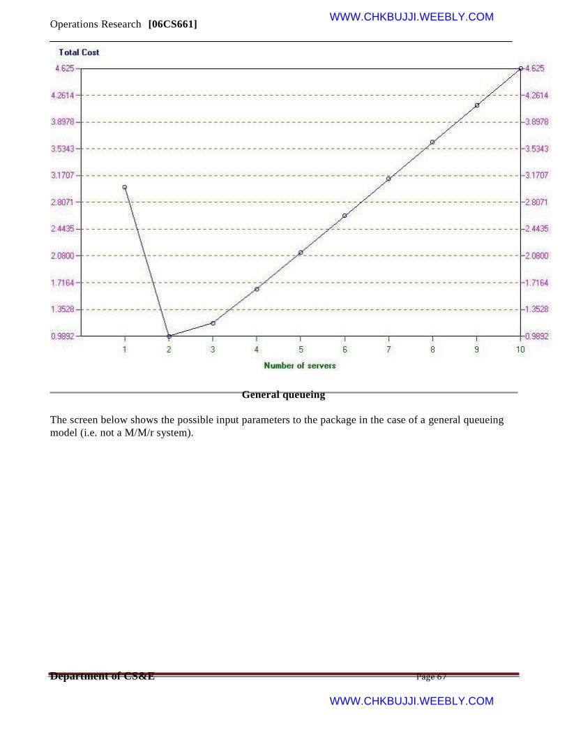
Operations Research [06CS661] WWW.CHKBUJJI.WEEBLY.COM
General queueing
The screen below shows the possible input parameters to the package in the case of a general queueing
model (i.e. not a M/M/r system).
Department of CS&E Page 67
WWW.CHKBUJJI.WEEBLY.COM
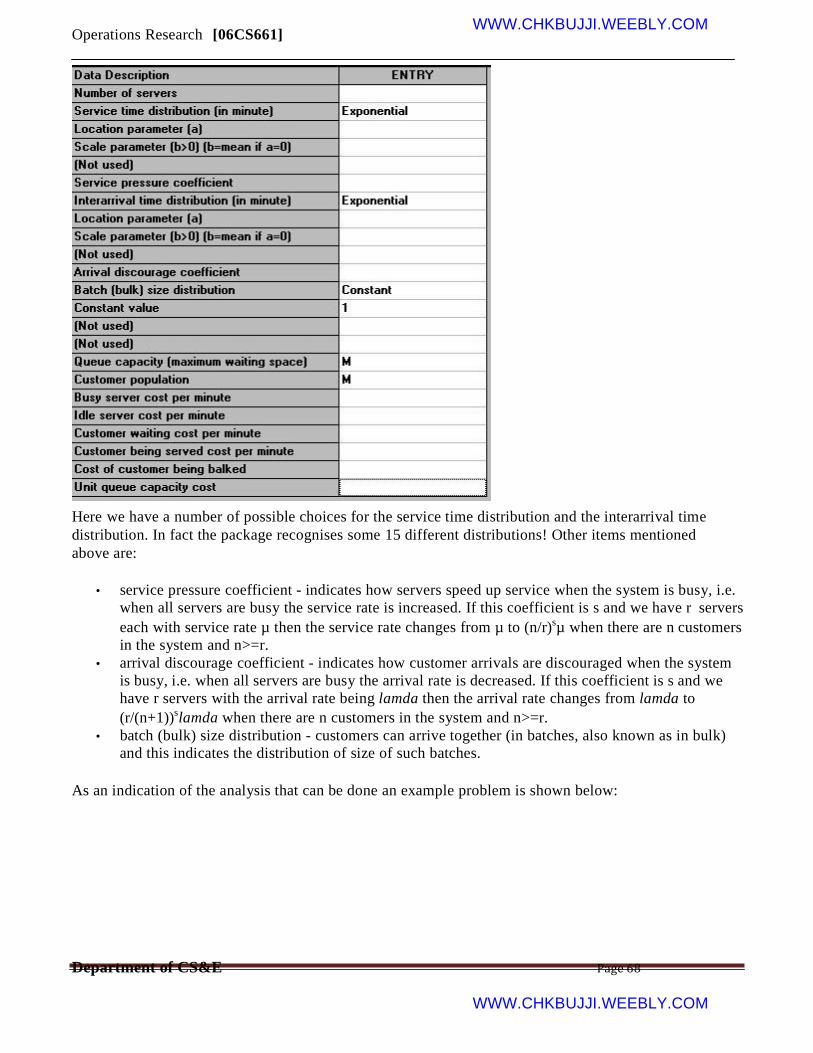
Operations Research [06CS661] WWW.CHKBUJJI.WEEBLY.COM
Here we have a number of possible choices for the service time distribution and the interarrival time
distribution. In fact the package recognises some 15 different distributions! Other items mentioned
above are:
• service pressure coefficient - indicates how servers speed up service when the system is busy, i.e.
when all servers are busy the service rate is increased. If this coefficient is s and we have r servers
each with service rate µ then the service rate changes from µ to (n/r)sµ when there are n customers
in the system and n>=r.
• arrival discourage coefficient - indicates how customer arrivals are discouraged when the system
is busy, i.e. when all servers are busy the arrival rate is decreased. If this coefficient is s and we
have r servers with the arrival rate being lamda then the arrival rate changes from lamda to
(r/(n+1))slamda when there are n customers in the system and n>=r.
• batch (bulk) size distribution - customers can arrive together (in batches, also known as in bulk)
and this indicates the distribution of size of such batches.
As an indication of the analysis that can be done an example problem is shown below:
Department of CS&E Page 68
WWW.CHKBUJJI.WEEBLY.COM
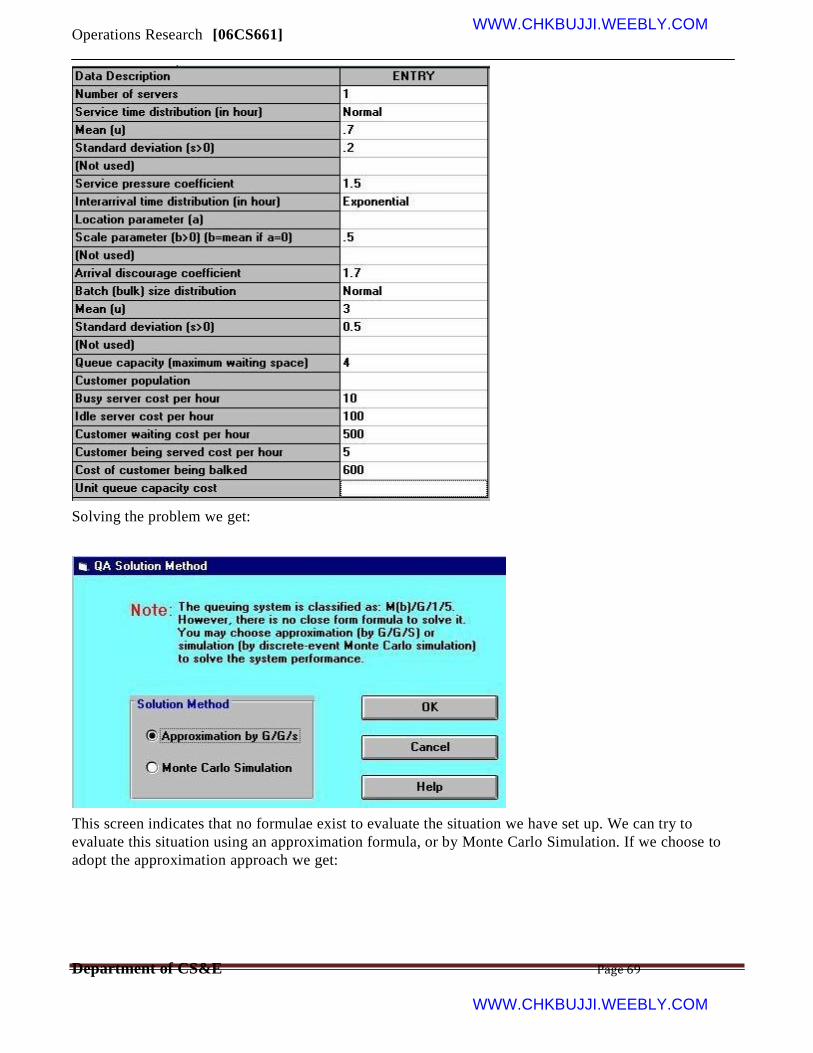
Operations Research [06CS661] WWW.CHKBUJJI.WEEBLY.COM
Solving the problem we get:
This screen indicates that no formulae exist to evaluate the situation we have set up. We can try to
evaluate this situation using an approximation formula, or by Monte Carlo Simulation. If we choose to
adopt the approximation approach we get:
Department of CS&E Page 69
WWW.CHKBUJJI.WEEBLY.COM

Operations Research [06CS661] WWW.CHKBUJJI.WEEBLY.COM
The difficulty is that these approximation results are plainly nonsense (i.e. not a good approximation). For
example the average number of customers in the queue is -2.9813, the probability that all servers are idle
is -320%, etc. Whilst for this particular case it is obvious that approximation (or perhaps the package) is
not working, for other problems it may not be readily apparent that approximation does not work.
If we adopt the Monte Carlo Simulation approach then we have the screen below.
Department of CS&E Page 70
WWW.CHKBUJJI.WEEBLY.COM

Operations Research [06CS661] WWW.CHKBUJJI.WEEBLY.COM
What will happen here is that the computer will construct a model of the system we have specified and
internally generate customer arrivals, service times, etc and collect statistics on how the system
performs. As specified above it will do this for 1000 time units (hours in this case). The phrase "Monte
Carlo" derives from the well-known gambling city on the Mediterranean in Monaco. Just as in roulette
we get random numbers produced by a roulette wheel when it is spun, so in Monte Carlo simulation we
make use of random numbers generated by a computer.
The results are shown below:
Department of CS&E Page 71
WWW.CHKBUJJI.WEEBLY.COM
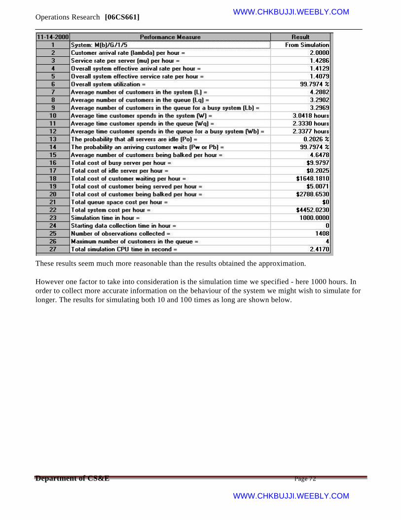
Operations Research [06CS661] WWW.CHKBUJJI.WEEBLY.COM
These results seem much more reasonable than the results obtained the approximation.
However one factor to take into consideration is the simulation time we specified - here 1000 hours. In
order to collect more accurate information on the behaviour of the system we might wish to simulate for
longer. The results for simulating both 10 and 100 times as long are shown below.
Department of CS&E Page 72
WWW.CHKBUJJI.WEEBLY.COM
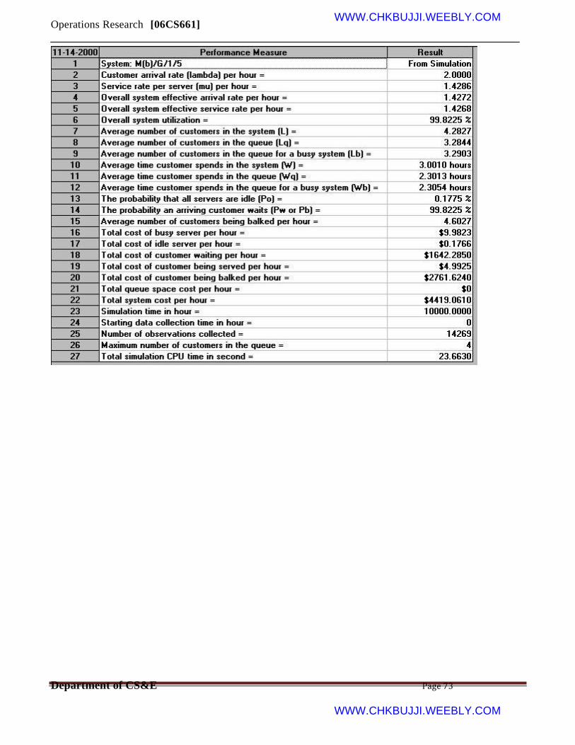
Operations Research [06CS661] WWW.CHKBUJJI.WEEBLY.COM
Department of CS&E Page 73
WWW.CHKBUJJI.WEEBLY.COM

Operations Research [06CS661] WWW.CHKBUJJI.WEEBLY.COM
Clearly the longer we simulate, the more confidence we may have in the statistics/probabilities obtained.
As before we can investigate how the system might behave with more servers. Simulating for 1000
hours (to reduce the overall elapsed time required) and looking at just the total system cost per hour
(item 22 in the above outputs) we have the following:
Number of servers Total system cost
1 4452
2 3314
3 2221
4 1614
5 1257
6 992
7 832
8 754
9 718
10 772
11 833
12 902
Hence here the number of servers associated with the minimum total system cost is 9
Department of CS&E Page 74
WWW.CHKBUJJI.WEEBLY.COM
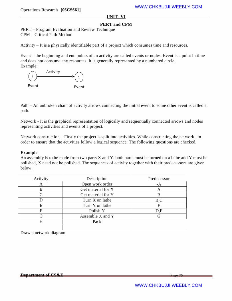
Operations Research [06CS661] WWW.CHKBUJJI.WEEBLY.COM
UNIT- VI
PERT and CPM
PERT – Program Evaluation and Review Technique
CPM – Critical Path Method
Activity – It is a physically identifiable part of a project which consumes time and resources.
Event – the beginning and end points of an activity are called events or nodes. Event is a point in time
and does not consume any resources. It is generally represented by a numbered circle.
Example:
Activity
i j
Event Event
Path – An unbroken chain of activity arrows connecting the initial event to some other event is called a
path.
Network - It is the graphical representation of logically and sequentially connected arrows and nodes
representing activities and events of a project.
Network construction – Firstly the project is split into activities. While constructing the network , in
order to ensure that the activities follow a logical sequence. The following questions are checked.
Example
An assembly is to be made from two parts X and Y. both parts must be turned on a lathe and Y must be
polished, X need not be polished. The sequences of activity together with their predecessors are given
below.
Activity
A
B
C
D
E
F
G
H
Description
Open work order
Get material for X
Get material for Y
Turn X on lathe
Turn Y on lathe
Polish Y
Assemble X and Y
Pack
Predecessor
-A
A
B
B,C
E
D,F
G
Draw a network diagram
Department of CS&E Page 75
WWW.CHKBUJJI.WEEBLY.COM
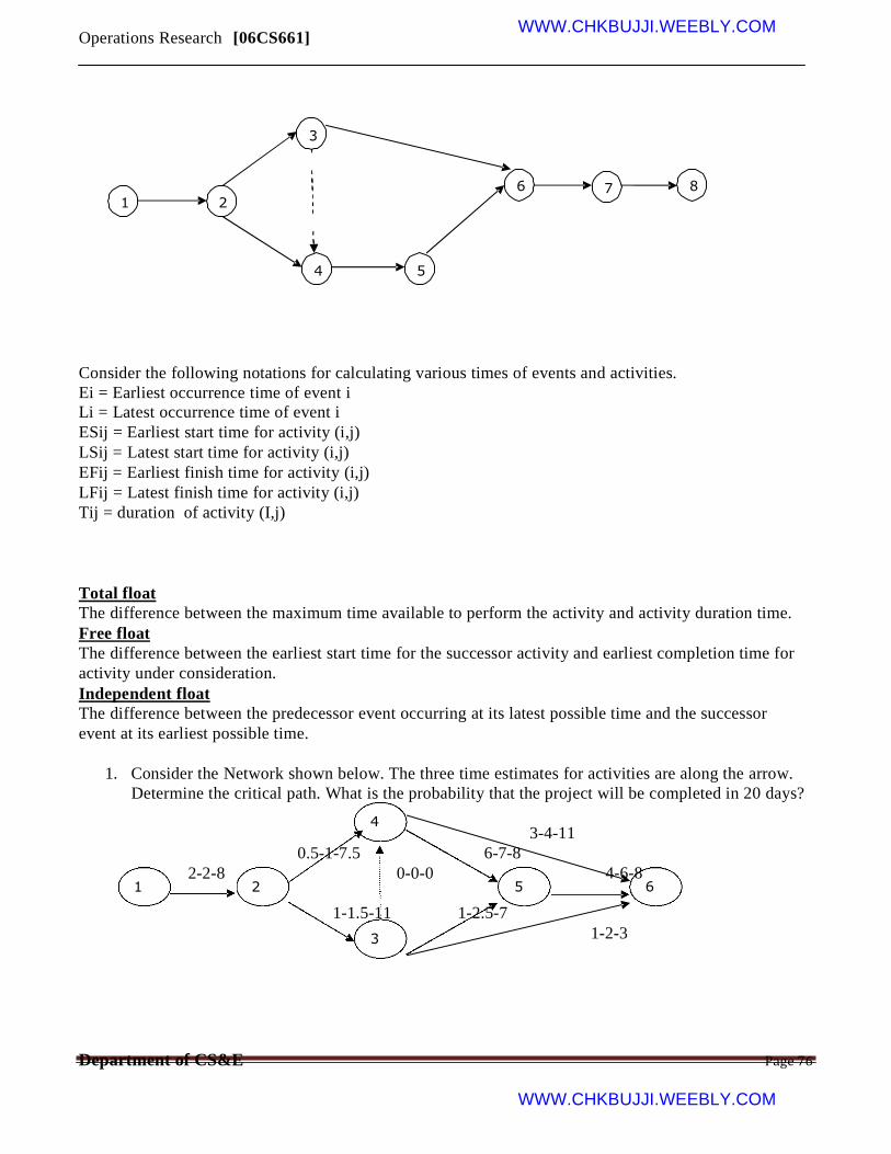
Operations Research [06CS661] WWW.CHKBUJJI.WEEBLY.COM
3
6 7 8
1 2
4 5
Consider the following notations for calculating various times of events and activities.
Ei = Earliest occurrence time of event i
Li = Latest occurrence time of event i
ESij = Earliest start time for activity (i,j)
LSij = Latest start time for activity (i,j)
EFij = Earliest finish time for activity (i,j)
LFij = Latest finish time for activity (i,j)
Tij = duration of activity (I,j)
Total float
The difference between the maximum time available to perform the activity and activity duration time.
Free float
The difference between the earliest start time for the successor activity and earliest completion time for
activity under consideration.
Independent float
The difference between the predecessor event occurring at its latest possible time and the successor
event at its earliest possible time.
1. Consider the Network shown below. The three time estimates for activities are along the arrow.
Determine the critical path. What is the probability that the project will be completed in 20 days?
4
0.5-1-7.5
1 2-2-8
2 0-0-0
3-4-11
6-7-8
5 4-6-8
6
1-1.5-11 1-2.5-7
3 1-2-3
Department of CS&E Page 76
WWW.CHKBUJJI.WEEBLY.COM

6
Operations Research [06CS661] WWW.CHKBUJJI.WEEBLY.COM
Te=6,tl=6
4
2
tl=3 7
te=0 te=3
1 3 2
Tl=0 3
2
3
5
5
3 Tl=13
te=13
te=19
tl=19
Te=6
Tl=6
V=[(tp-to)/6]2
Σ=2.08
z=Ts-Te/Σ
Z=0.48
From Std Dev. Probability = 68.44%
Crashing the network
Project crashing
Crashing is employed to reduce the project completion time by spending extra resources. Since for
technical reasons, time may not be reduced indefinitely, we call this limit crash point.
Cost slope = (crash cost - normal cost)/(normal time – crash time)
Example:
The following table gives data on normal time and cost and crash time and cost for a project.
Activity Normal Crash
Time(weeks) Cost
1-2 3 300
2-3 3 30
2-4 7 420
2-5 9 720
3-5 5 250
4-5 0 0
5-6 6 320
6-7 4 400
6-8 13 780
7-8 10 1000
Time(weeks) Cost
2 400
3 30
5 580
7 810
4 300
0 0
4 410
3 470
10 900
9 1200
Department of CS&E Page 77
WWW.CHKBUJJI.WEEBLY.COM

7
Operations Research [06CS661] WWW.CHKBUJJI.WEEBLY.COM
Indirect cost is Rs 50 per week. Crash the relevant activities systematically and determine the optimal
project completion time and cost.
Te=10,tl=12
te=22,tl=22 7
4
1 2 5 6
Te=0 te=3 te=12
Tl=0 tl=3 tl=12
3
te=18,tl=18
8
Te=6,tl=7 te=32
tl=32
e4=10 7
l4=11 4
1 3 2 0 6 5
4 6
10
e1=0 e2=3 9
l1=0 l2=3
e5=11 e6=17
l5=11 l6=17 13
3 3
5 8
e3=6
e8=31,l8=31
l3=6 new total cost = Rs 5815
e4=10 e7=19
l4=11 l7=19
4 10
Department of CS&E Page 78
1 2 5 6 WWW.CHKBUJJI.WEEBLY.COM
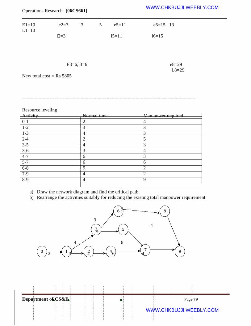
Operations Research [06CS661] WWW.CHKBUJJI.WEEBLY.COM
E1=10 e2=3 3 5 e5=11
L1=10
l2=3 l5=11
e6=15 13
l6=15
E3=6,l3=6 e8=29
L8=29
New total cost = Rs 5805
-----------------------------------------------------------------------------------------------------------
Resource leveling
Activity
0-1
1-2
1-3
2-4
3-5
3-6
4-7
5-7
6-8
7-9
8-9
Normal time
2
3
4
2
4
3
6
6
5
4
4
Man power required
4
3
3
5
3
4
3
6
2
2
9
a) Draw the network diagram and find the critical path.
b) Rearrange the activities suitably for reducing the existing total manpower requirement.
6 5
8
3
4 5
4
4 6
0 2 1
3 2 46 4
7 9
Department of CS&E Page 79
WWW.CHKBUJJI.WEEBLY.COM

Operations Research [06CS661] WWW.CHKBUJJI.WEEBLY.COM
3(3) 2(5) 6(3)
2(4) 4(3) 4(3) 6(6) 4(2)
3(4) 5(2) 4(9)
3(4) 5(2) 4(9)
1 2 3 4 5 6 7 8 9 10 11 12 13 14 15 16 17 18 19 20
4 4 6 6 6 8 12
4 4 6 6 6 8 8
10 10 8 11 11 11
10 10 10 9 11 11
8 15 15 11 11 2 2
8 8 8 11 11 11 11
Thus the man power is reduced to 11 people.
Deterministic Inventory Controls Model
An idle resource of any kind provides such as a resource has economic value. Such resources may be
classified into three categories
(i) Physical resources such as raw materials, semi-finished goods, finished goods, spare parts,
etc.
(ii) Human resources such as unused labor (man power).
(iii) Financial resource such as working capital, etc.
Economic order quantity (EOQ) for finding the optimum order quantity in order to balance costs to
balance costs of holding too much stock against that of ordering in small quantities too frequently.
Model: 1 (a) (Demand Rate Uniform production rate Infinite.)
R - Demand Rate
C3 – Setup cost per production (Cp)
Lead time is zero.
C1 – cost of holding one unit. (Ch)
Optimum interval,
T0= Sqrt(2C3/C1R)
Department of CS&E Page 80
WWW.CHKBUJJI.WEEBLY.COM

Operations Research [06CS661] WWW.CHKBUJJI.WEEBLY.COM
Optimum Quantity,
Q0=Rt0=Sqrt(2C3R/C1)
Minimum Average cost
C0= Sqrt(2C1.C3R)
Example:
A particular item has a demand of 9000 units/year. The of one procurement is Rs.100 and the holding
cost per unit is Rs.2.240 per year. The replacement is instantaneous & no shortages are allowed.
Determine,
(i)
(ii)
(iii)
(iv)
Solution
Economic lot size,
Number of orders per year,
Time between orders,
The total cost per year if the cost of one unit is Re1
R=9,000 units/year
C3= Rs. 100 /procurement,
C1= Rs 2.40 /unit/year
(i) q0 = Sqrt(2C3 R/ C1) = Sqrt(2*100*9000/2.40) = 866 units/procurement
(ii) N0=Sqrt(C1R/2C3) = Sqrt(2.40*9000/(2*100))= 10.4 orders/year
(iii) T0 = 1/N0 =1/10.4 = .0962 years between procurement.
(iv) C0=9000+Sqrt (2C1C3R)=9000+Sqrt(2*2.40*100*9000) =Rs 11080 /year
Model: 2 (a) (Demand Rate Uniform, Production Rate, Infinite, shortages Allowed)
This model is just the extension of model 1(a) allowing shortage .
C2 – Shortage cost per item per unit time. ( Cs )
Example
Solve the previous problem in addition to the data given that the problem the cost of shortage is also
given as Rs.5 per unit per year.
Solution
Department of CS&E Page 81
WWW.CHKBUJJI.WEEBLY.COM

Operations Research [06CS661] WWW.CHKBUJJI.WEEBLY.COM
R=9000
C3 = Rs 100 /procurement
C1 = Rs 2.40 /uit/procurement
C2 = Rs 5 /unit/year
(i) From Equation q0=Sqrt((C1+ C2)/ C2) * Sqrt(2C3R/ C1)=Sqrt((2.40+5)/5) *
Sqrt((2*100*9000)/2.4) =1053 units/run
(ii) C0(Im,q) = 9000*1+Sqrt(C2(C2+ C1))*Sqrt(2C1C3R) = 10710 /year
(iii)Number of orders/year
N0=9000/1053 = 8.55
(iv)Time between orders,
t0=1/N0 =1/8.55 =0.117 year
Example
The demand for a commodity is 100 units per day. Every time an order is placed, a fixed cost Rs. 400 is
incurred. Holding cost is Rs 0.08 per unit per day. If the lead time is 13 days, determine the economic lot
size & the reorder point
Solution
Q0=Sqrt(2C3R/ C3)=Sqrt(2*4*100/0.08) = 1000 units.
Length of the cycle t0 = 1000/100 =10 days.
As the lead time is 13 days & the cycle length is 10 days, recording should occur when the leve of
inventory is sufficient to satisfy the demand for 13-10 = 3 days
� Reorder point =100*3 = 300 units.
It may be noted that the ‘effective’ lead time is taken equal to 3 days rather than 13 days. It is because
the lead time is longer than t0.
Model1(b) (Demand Rate Non-uniform, production Rate Infinite)
In this method all assumptions are same as in model 1(a) with the exception that instead of uniform
demand rate R, we are given some total amount D, to be satisfied during some long time period T. Thus,
demand rates are different in different production runs
Optimal Lot size q0 = Sqrt(2C3(D/T)/C1)
And minimum total cost, C0(q) = Sqrt(2C1C3(D/T))
Here, it can be noted that the uniform demand rate R in model 1(a) is replaced by average demand rate
D/T.
Example
Department of CS&E Page 82
WWW.CHKBUJJI.WEEBLY.COM
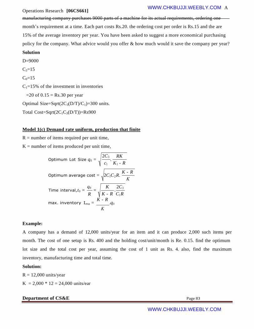
.
. q
Operations Research [06CS661] WWW.CHKBUJJI.WEEBLY.COM A
manufacturing company purchases 9000 parts of a machine for its actual requirements, ordering one
month’s requirement at a time. Each part costs Rs.20. the ordering cost per order is Rs.15 and the are
15% of the average inventory per year. You have been asked to suggest a more economical purchasing
policy for the company. What advice would you offer & how much would it save the company per year?
Solution
D=9000
C3=15
C0=15
C1=15% of the investment in inventories
=20 of 0.15 = Rs.30 per year
Optimal Size=Sqrt(2C3(D/T)/C1)=300 units.
Total Cost=Sqrt(2C1C3(D/T))=Rs900
Model 1(c) Demand rate uniform, production that finite
R = number of items required per unit time,
K = number of items produced per unit time,
Optimum Lot Size q0 = 2C3 RK
c1 K1 - R
Optimum average cost = 2C1C2R. K - R
Time interval,t0 = R
= K 2C3
K - R C1R
max. inventory Imo = K - R
.q0
Example:
A company has a demand of 12,000 units/year for an item and it can produce 2,000 such items per
month. The cost of one setup is Rs. 400 and the holding cost/unit/month is Re. 0.15. find the optimum
lot size and the total cost per year, assuming the cost of 1 unit as Rs. 4. also, find the maximum
inventory, manufacturing time and total time.
Solution:
R = 12,000 units/year
K = 2,000 * 12 = 24,000 units/ear
Department of CS&E Page 83
WWW.CHKBUJJI.WEEBLY.COM
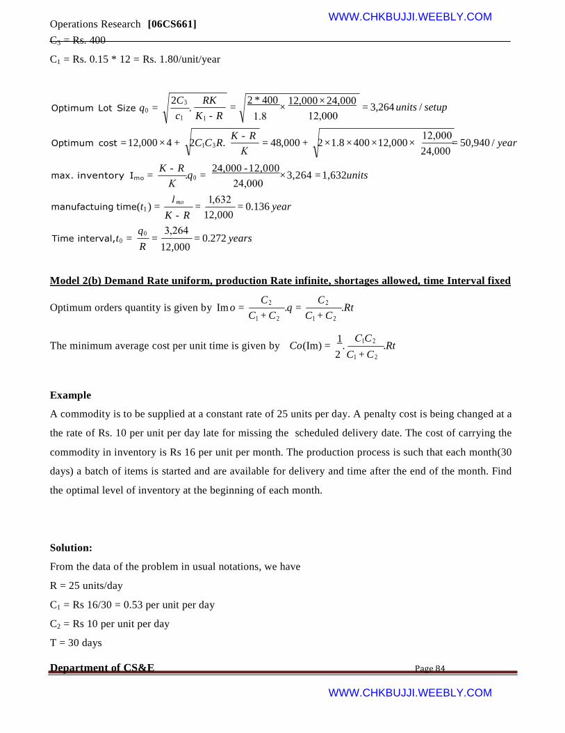
.
q
C C
C 1
Operations Research [06CS661] WWW.CHKBUJJI.WEEBLY.COM
C3 = Rs. 400
C1 = Rs. 0.15 * 12 = Rs. 1.80/unit/year
Optimum Lot Size q0 = 2C3 RK
c1 K1 - R
= 2 * 400
× 12,000 × 24,000
= 3,264 units / setup
Optimum cost =12,000 ×4 + 2C1C3R. K - R
= 48,000 + 2 ×1.8 ×400 ×12,000 × 24,000
= 50,940 / year
max. inventory Imo = K - R
.q0 = 24,000 -12,000
×3,264 =1,632units
manufactuing time(t1) = K - R
= 12,000
= 0.136 year
Time interval,t0 = R
= 12,000
= 0.272 years
Model 2(b) Demand Rate uniform, production Rate infinite, shortages allowed, time Interval fixed
Optimum orders quantity is given by Im o = C1 + C 2
.q = C1 + C2
.Rt
The minimum average cost per unit time is given by Co(Im) = 2
.C1 + C 2
.Rt
Example
A commodity is to be supplied at a constant rate of 25 units per day. A penalty cost is being changed at a
the rate of Rs. 10 per unit per day late for missing the scheduled delivery date. The cost of carrying the
commodity in inventory is Rs 16 per unit per month. The production process is such that each month(30
days) a batch of items is started and are available for delivery and time after the end of the month. Find
the optimal level of inventory at the beginning of each month.
Solution:
From the data of the problem in usual notations, we have
R = 25 units/day
C1 = Rs 16/30 = 0.53 per unit per day
C2 = Rs 10 per unit per day
T = 30 days
Department of CS&E Page 84
WWW.CHKBUJJI.WEEBLY.COM

5
� �
� �
Operations Research [06CS661] WWW.CHKBUJJI.WEEBLY.COM
The optimal inventory level is given by = �
0.53 +10� ×25 ×30 = 712units
Model 2(c) Demand Rate uniform, production Rate finite, shortage allowed
This model has the same assumptions as in model 2(a) except that production rate is finite.
Example
Find the results of example 12.5 –2 if in addition to the date given in that problem the cost of shortages
is also given as Rs. 5 per unit per year.
Solution
R = 9,000 units/year
C3 = Rs. 100 / procurement,
C1 = Rs. 2.40 / unit/year
C2 = Rs. 5/ unit/year
i) qo = C1 + C2 2C3 R
C 2 C1
2.40 + 5 .
2 ×100 ×9000
2.4
=1053
ii) Co(Im, q) = 9000 ×1 + C 2
C1 + C2
2C1C3R = 9000 +
5
2.4 + 5
2 ×2.4 ×100 ×9000 =10710 years
iii) Number of orders/year, N 0 = 1053
= 8.55
iv) Time between orders, to
= N
0
= 8.55
= 0.117 year
Notes:
Department of CS&E Page 85
WWW.CHKBUJJI.WEEBLY.COM
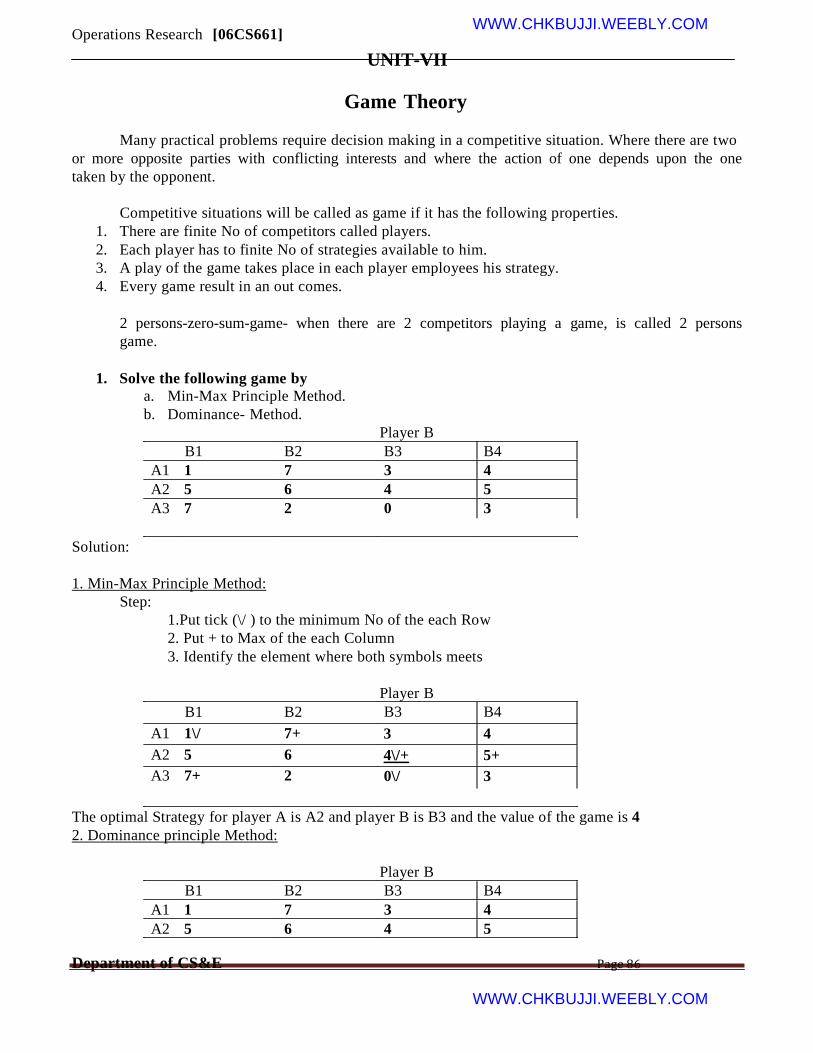
Operations Research [06CS661] WWW.CHKBUJJI.WEEBLY.COM
UNIT-VII
Game Theory
Many practical problems require decision making in a competitive situation. Where there are two
or more opposite parties with conflicting interests and where the action of one depends upon the one
taken by the opponent.
Competitive situations will be called as game if it has the following properties.
1. There are finite No of competitors called players.
2. Each player has to finite No of strategies available to him.
3. A play of the game takes place in each player employees his strategy.
4. Every game result in an out comes.
2 persons-zero-sum-game- when there are 2 competitors playing a game, is called 2 persons
game.
1. Solve the following game by
a. Min-Max Principle Method.
b. Dominance- Method.
Player B
B1 B2 B3 B4
A1 1 7 3 4
A2 5 6 4 5
A3 7 2 0 3
Solution:
1. Min-Max Principle Method:
Step:
1.Put tick (\/ ) to the minimum No of the each Row
2. Put + to Max of the each Column
3. Identify the element where both symbols meets
B1 B2
A1 1\/ 7+
A2 5 6
A3 7+ 2
Player B
B3 B4
3 4
4\/+ 5+
0\/ 3
The optimal Strategy for player A is A2 and player B is B3 and the value of the game is 4
2. Dominance principle Method:
Player B
B1 B2 B3 B4
A1 1 7 3 4
A2 5 6 4 5
Department of CS&E Page 86
WWW.CHKBUJJI.WEEBLY.COM

Operations Research [06CS661] WWW.CHKBUJJI.WEEBLY.COM A3 7 2 0
3
Steps:
1. Row Comparison Inferiors.
2. Column comparison Superior.
1. The elements of the second column are superior to corresponding elements of 3rd column so
delete II column.
The revised matrix is:
Sol: Player B
B1 B3 B4
A1 1 3 4
A2 5 4 5
A3 7 0 3
2. The elements of I row are inferior to corresponding elements of II rows So Delete I row (A1)
The revised matrix is:
Sol: Player B
B1 B3 B4
A2 5 4 5
A3 7 0 3
3. B1 is superior to B3 Delete B1.
The revised matrix is :
Sol: Player B
B3 B4
A2 4 5
A3 0 3
4. A3 is inferior to A2 – Delete A3
The revised matrix is :
Sol: Player B
B3 B4
A2 4 5
4. B4 is superior is to B3 Delete B4
The revised matrix is :
Sol: Player B
B3
A2 4
The optimal strategy for player A is A2 and B is B3
The Value of the Game is 4
2. Solve the following game.
Player B
Department of CS&E Page 87
WWW.CHKBUJJI.WEEBLY.COM
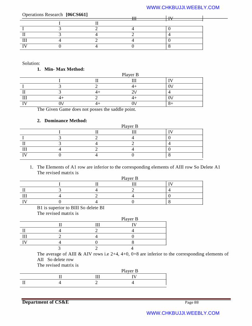
Operations Research [06CS661]
I II
WWW.CHKBUJJI.WEEBLY.COM
III IV
I 3 2 4 0
II 3 4 2 4
III 4 2 4 0
IV 0 4 0 8
Solution:
1. Min- Max Method:
I II
I 3 2
II 3 4+
III 4+ 2
IV 0\/ 4+
Player B
III IV
4+ 0\/
2\/ 4
4+ 0\/
0\/ 8+
The Given Game does not posses the saddle point.
2. Dominance Method:
I II
I 3 2
II 3 4
III 4 2
IV 0 4
Player B
III IV
4 0
2 4
4 0
0 8
1. The Elements of A1 row are inferior to the corresponding elements of AIII row So Delete A1
The revised matrix is
Player B
I II III IV
II 3 4 2 4
III 4 2 4 0
IV 0 4 0 8
B1 is superior to BIII So delete BI
The revised matrix is
Player B
II III IV
II 4 2 4
III 2 4 0
IV 4 0 8
3 2 4
The average of AIII & AIV rows i.e 2+4, 4+0, 0+8 are inferior to the corresponding elements of
AII So delete row
The revised matrix is
Player B
II III IV
II 4 2 4
Department of CS&E Page 88
WWW.CHKBUJJI.WEEBLY.COM
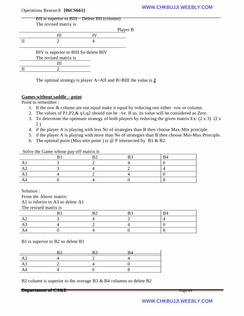
Operations Research [06CS661] WWW.CHKBUJJI.WEEBLY.COM
BII is superior to BIII – Delete BII (column)
The revised matrix is
Player B
III IV
II 2 4
BIV is superior to BIII So delete BIV
The revised matrix is
III
II 2
The optimal strategy is player A=AII and B=BIII the value is 2
Games without saddle – point
Point to remember :
1. If the row & column are not equal make it equal by reducing one either row or column.
2. The values of P1,P2,& q1,q2 should not be –ve. If so, its value will be considered as Zero.
3. To determine the optimum strategy of both players by reducing the given matrix Ex: (2 x 3) (2 x
2 )
4. if the player A is playing with less No of strategies than B then choose Max-Min principle.
5. if the player A is playing with more than No of strategies than B then choose Min-Max Principle.
6. The optimal point (Max-min point ) is @ P intersected by B1 & B2.
Solve the Game whose pay-off matrix is
B1 B2 B3 B4
A1 3 2 4 0
A2 3 4 2 4
A3 4 2 4 0
A4 0 4 0 8
Solution :
From the Above matrix:
A1 is inferior to A3 so delete A1
The revised matrix is
B1 B2 B3 B4
A2 3 4 2 4
A3 4 2 4 0
A4 0 4 0 8
B1 is superior to B2 so delete B1
B2 B3 B4
A2 4 2 4
A3 2 4 0
A4 4 0 8
B2 column is superior to the average B3 & B4 columns so delete B2
Department of CS&E Page 89
WWW.CHKBUJJI.WEEBLY.COM

Operations Research [06CS661] WWW.CHKBUJJI.WEEBLY.COM
The revised matrix is:
B3 B4
A2 2 4
A3 4 0
A4 0 8
A2 is inferior to the average of A3 and A4 rows so delete A4
The revised matrix is:
B3 B4
A34 0
A4 0 8
Further the games has no saddle point.
B3 B4
A3 a11 a12
A4 a21 a22
Let the players A chooses his strategies A3, A4 with probabilities P1 & P2. Such that P1+P2=1.
Similarly player B chooses his strategies B3+B4 with probabilities q1 &q2, such that q1+q2=1.
Formula
P1= a22-a21
a11+a22-(a12+a21)
q1= a22-a12
a11+a22-(a12+a21)
Value of the Game= a11 x a22-a12 x a21
a11+a22-(a12+a21)
P1= a22-a21
a11+a22-(a12+a21)
= 8-0
4+8-(0+0)
= 8
12
=0.67
P1+P2=1 We know the value of P1=067 so when we substitute we get P2=1-067 P2=0.33
q1= a22-a12
a11+a22-(a12+a21)
Department of CS&E Page 90
WWW.CHKBUJJI.WEEBLY.COM
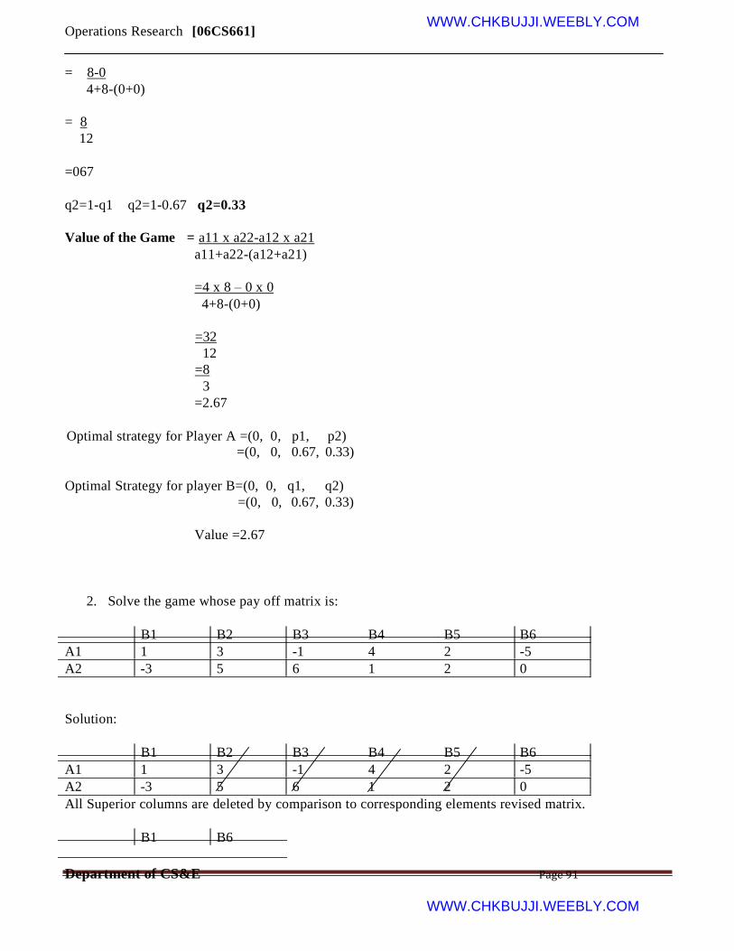
Operations Research [06CS661] WWW.CHKBUJJI.WEEBLY.COM
= 8-0
4+8-(0+0)
= 8
12
=067
q2=1-q1 q2=1-0.67 q2=0.33
Value of the Game = a11 x a22-a12 x a21
a11+a22-(a12+a21)
=4 x 8 – 0 x 0
4+8-(0+0)
=32
12
=8
3
=2.67
Optimal strategy for Player A =(0, 0,
=(0, 0,
p1, p2)
0.67, 0.33)
Optimal Strategy for player B=(0, 0, q1, q2)
=(0, 0, 0.67, 0.33)
Value =2.67
2. Solve the game whose pay off matrix is:
B1 B2 B3 B4 B5 B6
A1 1 3 -1 4 2 -5
A2 -3 5 6 1 2 0
Solution:
B1 B2 B3 B4 B5 B6
A1 1 3 -1 4 2 -5
A2 -3 5 6 1 2 0
All Superior columns are deleted by comparison to corresponding elements revised matrix.
B1 B6
Department of CS&E Page 91
WWW.CHKBUJJI.WEEBLY.COM
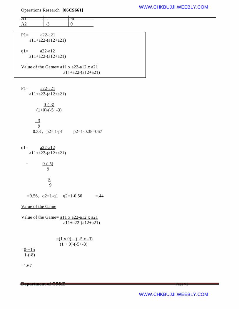
Operations Research [06CS661] WWW.CHKBUJJI.WEEBLY.COM
A1 1 -5
A2 -3 0
P1= a22-a21
a11+a22-(a12+a21)
q1= a22-a12
a11+a22-(a12+a21)
Value of the Game= a11 x a22-a12 x a21
a11+a22-(a12+a21)
P1= a22-a21
a11+a22-(a12+a21)
= 0-(-3)
(1+0)-(-5+-3)
=3
9
0.33 , p2= 1-p1 p2=1-0.38=067
q1= a22-a12
a11+a22-(a12+a21)
= 0-(-5)
9
= 5
9
=0.56, q2=1-q1 q2=1-0.56 =.44
Value of the Game
Value of the Game= a11 x a22-a12 x a21
a11+a22-(a12+a21)
=(1 x 0) – ( -5 x -3)
(1 + 0)-(-5+-3)
=0-+15
1-(-8)
=1.67
Department of CS&E Page 92
WWW.CHKBUJJI.WEEBLY.COM
Operations Research
A1
[06CS661]
A2
WWW.CHKBUJJI.WEEBLY.COM B1 B2
7 7 7 7
6 6 6 6
5 5 5 5
4 4 4 P 4
3 3 3 3
2 2 2 2
1 1 1 1
-1 -1 -1 -1
-2 -2 -2 -2
-3 -3 -3 -3
p -4 -4 -4
-4 -5 -5 -5
-5 -6 -6 -6
-6 -7 -7 -7
-7
Department of CS&E Page 93
WWW.CHKBUJJI.WEEBLY.COM

Operations Research [06CS661] WWW.CHKBUJJI.WEEBLY.COM
UNIT - VIII
Integer Programming
The replacement problem arises because of two factors:
1. First, the existing unit or units may have outlived their effective lives and it may not be
economical to allow them to continue in the organization.
2. Second, the existing unit or units may have been destroyed through accident or otherwise.
In the case of items whose efficiency go on decreasing according to their, it requires to spend more
money on account of increased operating cost, increased repair cost, increased scrap, etc. In such
cases the replacement of an old item with new one is the only alternative to prevent such increased
expenses. Thus, it becomes necessary to determine an age at which replacement is more economical
rather than to continue at increased cost. The problems of replacements are encountered in the case
of both men and machines. By applying probability it is possible to estimate the chance of death at
various ages.
Types of replacement problems:
1. Replacement of capital equipment that becomes worse with time, e.g. machines tools, buses in a
transport organization, planes, etc
2. Group replacement of items which fail completely, e.g. light bulbs, radio tubes, etc.
3. Problems of mortality and staffing.
4. Miscellaneous problems.
1. The cost of machine is Rs 6100 and its scrap value is only Rs 100. The maintenance costs are
found from experience to be:
Year 1 2 3 4 5
Mtn- 100 250 400 600 900
Cost
6 7 8
1250 1600 2000
When should the machine be replace?
Solution:
First, find an average cost per year during the life of the machine as follows.
These computations may be summarized in the following
Replace at
the end of
the year (n)
(n)
1
2
3
4
5
6
7
Maintenance
cost an
Rn
100
250
400
600
900
1250
1600
Total
maintenance
cost
∑
100
350
750
1350
2250
3500
4100
Difference
b/w Price
and Resale
price
(c-s)
6000
6000
6000
6000
6000
6000
6000
Total cost
[p(n)]
6100
6350
6750
7350
8250
9500
11100
Average cost
P(n)/n
6100
3175
2250
1837.50
1650
1583.33
1585.71
Department of CS&E Page 94
WWW.CHKBUJJI.WEEBLY.COM

Operations Research [06CS661] WWW.CHKBUJJI.WEEBLY.COM
Here it is observed that the maintenance cost in the 7th year becomes greater than the average cost
for 6 years. Hence the machine should be replaced at the end of 6th year.
2. Machine owner finds from his past records that the costs per year of maintaining a machine
whose purchase price is Rs 6000 are as given below:
Year 1 2
Mtn 1000 1200
Cost
Resale 3000 1500
price
3 4
1400 1800
750 375
5 6 7 8
2300 2800 3400 4000
200 200 200 200
At what age is a replacement due?
Solution: As in example 1, the machine should be replace at the end of the fifth year, because the
maintenance cost in the 6th year becomes greater than the average cost for 5 years.
Here the average cost per year during the life of the machine.
Replace at
the end of
year (n)
(n)`
1
2
3
4
5
6
Maintenance
cost
Rn
1000
1200
1400
1800
2300
2800
Total
maintenance
cost
∑Rn
1000
2200
3600
5400
7700
10500
Difference
b/w price
and resale
price
(c-sn)
3000
4500
5250
5625
5800
5800
Total cost
P(n)
4000
6700
8850
11025
13500
16300
Average cost
P(n)/n
4000
3350
2950
2756
2700
2717
1. An Engineering company is offered a material handling equipment A. A is priced at Rs.60,000.
including cost of installation; and the cost for operation and maintenance are estimated to be Rs. 10,000
for each of the first five years, increasing every year by Rs.3,000 per year in the sixth and subsequent
years. The company expects a return of 10% on all its investment. What is the optimal replacement
period?
Year n Running
cost Rn
(1) (2)
1 1,000
2 11,000
3 21,000
4 31,000
5 41,000
6 51,000
Year n Running
cost Rn
Cumulative
running
cost
(3)
1,000
12000
33000
64000
1051000
156000
Cumulative
running
Depreciation
cost
(4)
45000
45000
45000
45000
45000
45000
Depreciation
cost
TC
(3+4)
46000
57000
78000
109000
150000
2,01000
TC
ATC
(5)/(1)
46000
28500
26000
27250
30000
33500
ATC
Department of CS&E Page 95
WWW.CHKBUJJI.WEEBLY.COM

Operations Research [06CS661] WWW.CHKBUJJI.WEEBLY.COM
cost
(1) (2) (3) (4)
1 2,000 2,000 50000
2 6,000 8000 50000
3 10,000 18000 50000
4 14,000 32000 50000
5 18,000 50000 50000
6 22,000 72000 50000
(3+4)
52000
58000
68000
829000
100000
1,22,000
(5)/(1)
52000
29000
22667
20500
20000
20333
A should be replaced by
2. A computer contains 10,000 resistors. When any resistor fails, it is replaced. The cost
of replacing a resistor individually is Re.1 only. If all the resistors are replaced at the
same time, the cost per resistor would be reduced to 35 paise. The percentage of
surviving resistors say S(t) at the end of month t and P(t) the probability of failure
during the month t are:
T 0
S(t) 100
P(t) -
1 2
97 90
0.03 0.07
3 4 5 6
70 30 15 0
0.20 0.40 0.15 0.15 What is the optimal replacement plan?
No=10,000
N1=300
N2=709
N3=2042
N4=4171
N5=2030
N6=2590
Expected life = 4.02 months
Avg Failures = 2488 resistors
End of month TC
1 3,800
2 4,509
3 6,551
4 10,722
5 12,752
6 15,442
ATC
380,00
2254.50
2183.66
2680.5
2550.40
2557.00
3. Machine A costs Rs.45,000 and the operating costs are estimated at Rs.1000 for the first year
increasing by Rs.10,000 per year in the second and subsequent years. Machine B costs Rs.50,000 and
operating costs are Rs.2,000 for the first year, increasing by Rs.4,000 in the second and subsequent
years. If we now have a machine of type A, should we replace it with B? If so when? Assume that both
machines have no resale value and future costs are not discounted.
Year n Running Discounted Rn Dn- Cummulative C+cummulative C W(n)
Department of CS&E Page 96
WWW.CHKBUJJI.WEEBLY.COM

Operations Research
cost Rn
[06CS661] WWW.CHKBUJJI.WEEBLY.COM
factor Dn-1 1
(1) (2) (3)
1 10,000 .909
2 10,000 .826
3 10,000 .757
4 10,000 .683
5 10,000 .621
6 13,000 .564
7 16,000 .513
8 19,000 .466
9 22,000 .424
10 25,000 .385
(2)*(3) (5)
9,090 9,090
8,260 17,350
7,510 24,860
6,830 31,690
6,210 37,900
7,332 45,232
8,208 53,440
8,854 62,294
9,328 71,622
9,650 81,247
60,000+(5)
69,090
77,350
84,860
91,690
97,900
1,05,232
1,13,440
1,22,294
1,31,622
1,41,247
(7) (6)/(7)
.909 36,192
1.735 28,282
2.486 24,343
4.169 21,993
4.790 20,438
5.354 19,655
5.867 19,335
6.333 19,311
6.757 19,479
7.142 19,777
Department of CS&E Page 97
WWW.CHKBUJJI.WEEBLY.COM
Related Documents