Operations Research for Healthcare ‐ lecture notes (Part 3 ...

Operations Research for Healthcare ‐lecture notes (Part 3)

IUMS‐1397

© Dr. Ahmad Reza Pourghaderi 1

OPERATIONS RESEARCH for HEALTHCARE

(Part 3)SOLUTION METHODS

AHMAD REZA POURGHADERI (PH .D. )

ASS ISTANT PROFESSOR OF HEALTHCARE SYSTEMS ENGINEERING

ISFAHAN UNIVERS ITY OF MEDICAL SC IENCES

HTTP : / /POURGHADERI .COM/

Part : Learning Objectives

Giving a general understanding of a variety of methods to solve MP models.

Discuss the complexity of solving a mathematical programming model and introduce

tractable (easy) versus intractable (NP) problems.

Describe two main solution approaches: Exact and Approximate algorithms.

Introduce the main exact algorithms for LP and IP models.

Introduce several famous metaheuristic methods and categorize them in two groups

of single‐solution and population‐based.

Explain post optimality (what‐if) analysis and highlight the sensitivity analysis.

Explain the concepts of robust optimization.

2ISFAHAN UNIVERSITY OF MEDICAL SCIENCE ‐ DEPARTMENT OF HEALTHCARE OPERATIONS MANAGEMENT DR. AHMAD REZA POURGHADERI – POURGHADERI.COM

After a mathematical model is formulated for the problem under consideration,

the next phase in an OR study is to develop a procedure (usually a computer‐

based procedure) for deriving solutions to the problem from this model.

You might think that this must be the major part of the study, but actually it is

not in most cases. Sometimes, in fact, it is a relatively simple step, in which one

of the standard algorithms (systematic solution procedures) of OR is applied on a

computer by using one of a number of readily available software packages.

DERIVING SOLUTIONS FROM THE MODEL



IUMS‐1397


A common theme in OR is the search for an optimal, or best solution.

It needs to be recognized that these solutions are optimal only with respect to

the model being used. Since the model necessarily is an idealized rather than an

exact representation of the real problem, there cannot be any utopian

guarantee that the optimal solution for the model will prove to be the best

possible solution that could have been implemented for the real problem.

If the model is well formulated and tested, the resulting solution should tend to

be a good approximation to an ideal course of action for the real problem.

DERIVING SOLUTIONS FROM THE MODEL


Exact Vs Approximate Solution Algorithms

Exact algorithms can find the optimum solution with precision.

Approximate algorithms can find a near optimum solution.

The main difference is that exact algorithms apply in "easy (tractable)"

problems. What makes a problem "easy" is that it can be solved in

reasonable time and the computation time doesn't scale up exponentially

if the problem gets bigger. This class of problems is known

as P(Deterministic Polynomial Time). Problems of this class are used to be

optimized using exact algorithms. For every other class of problems (NP‐

hard, NP‐Complete) approximate algorithms are preferred.


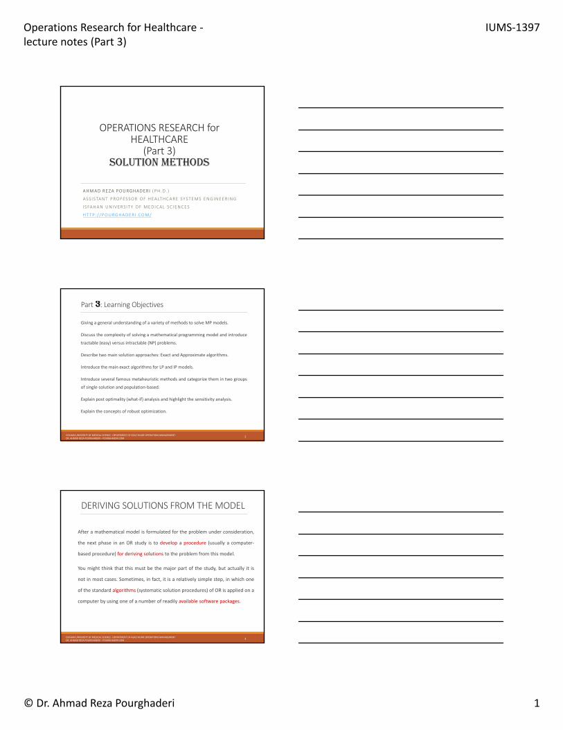
Types of Mathematical ProgrammingName Vars Constraints Objective

constraint programming discrete? any N/A

linear programming (LP) real linear inequalities linear function

integer linear prog. (ILP) integer linear inequalities linear function

mixed integer prog. (MIP) int&real linear inequalities linear function

quadratic programming real linear inequalities quadratic function

semidefinite programming real linear inequalities +semidefiniteness

linear function

quadratically constrained programming

real quadratic inequalities linear or quadraticfunction

convex programming real convex region convex function

nonlinear programming real any any

For each type of above MPs, there exists specific exact algorithms which provide optimal

solutions (usually under some conditions). LP and MIP examples are given in the next few

slides6

ISFAHAN UNIVERSITY OF MEDICAL SCIENCE ‐ DEPARTMENT OF HEALTHCARE OPERATIONS MANAGEMENT DR. AHMAD REZA POURGHADERI – POURGHADERI.COM


IUMS‐1397


7

• Simplex Algorithm: It is developed by George Dantzig in 1947, solves LP

problems by constructing a feasible solution at a vertex of the polytope and

then walking along a path on the edges of the polytope to vertices with non-

decreasing values of the objective function until an optimum is reached for

sure.

• Criss‐cross Algorithm: It is like the Simplex a basis-exchange algorithm that

pivots between bases. However, the criss-cross algorithm need not maintain

feasibility, but can pivot rather from a feasible basis to an infeasible basis.

• Interior point Algorithm: In contrast to the simplex algorithm, which finds an

optimal solution by traversing the edges between vertices on a polyhedral

set, interior-point methods move through the interior of the feasible region.

• Other LP algorithms: Karmarkar's algorithm, Khachiyan's algorithm, …


8

The current opinion is that the efficiencies of good implementations of

simplex‐based methods are the best similar for routine applications of linear

programming.

However, for specific types of LP problems, it may be that one type of solver is

better than another (sometimes much better).

The structure of the solutions generated by interior point methods versus

simplex‐based methods are significantly different with the support set of active

variables being typically smaller for the later one.


9

One class of algorithms are Cutting Plane methods which work by solving the LP

relaxation and then adding linear constraints that drive the solution towards

being integer without excluding any integer feasible points.

Another class of algorithms are variants of the branch and bound method. A B&B

algorithm consists of a systematic enumeration of candidate solutions. Before

enumerating the candidate solutions of a branch, the branch is checked against

upper and lower estimated bounds on the optimal solution, and is discarded if it

cannot produce a better solution than the best one found so far by the algorithm.

the branch and cut method that combines both branch and bound and cutting

plane methods.



IUMS‐1397


Approximate Algorithms

Heuristic procedures (i.e., intuitively designed procedures that do not

guarantee an optimal solution) to find a good sub‐optimal solution.

This is most often the case when the time or cost required to find an

optimal solution for an adequate model of the problem would be very

large. In recent years, great progress has been made in developing

efficient and effective heuristic procedures (including so‐called

metaheuristics), so their use is continuing to grow.


Herbert Simon (Nobel Laureate in economics) points out that satisficing is much more

prevalent than optimizing in actual practice.

Satisficing Theory (Simon 1947) is a decision‐making strategy that entails searching through

the available alternatives until an acceptability threshold is met.

Simon is describing the tendency of managers to seek a solution that is “good enough” for

the problem at hand. Rather than trying to develop an overall measure of performance to

optimally reconcile conflicts between various desirable objectives.

One of England’s OR leaders, Samuel Eilon, “Optimizing is the science of the ultimate;

satisficing is the art of the feasible.

Satisficing vs Optimizing


Imagination is more important than

knowledge, for knowledge is limited

Whereas imagination embrace the entire

world, stimulating progress giving birth to

evolution.

Albert Einstein


IUMS‐1397


Metaheuristic Algorithms

A metaheuristic is a higher‐level procedure or heuristic designed to find, generate, or

select a heuristic (partial search algorithm) that may provide a sufficiently good solution

to an optimization problem, especially with incomplete or imperfect information or

limited computation capacity.

These are properties that characterize most metaheuristics:

Metaheuristics are strategies that guide the search process.

The goal is to efficiently explore the search space in order to find near–optimal solutions.

Techniques which constitute metaheuristic algorithms range from simple local search

procedures to complex learning processes.

Metaheuristic algorithms are approximate and usually non‐deterministic.

Metaheuristics are not problem‐specific.


Single‐solution vs Population‐based Metaheuristics

Single solution approaches focus on modifying and improving a single

candidate solution; single solution metaheuristics include simulated

annealing, Tabu search, iterated local search, variable neighborhood

search, and guided local search.

Population‐based approaches maintain and improve multiple candidate

solutions, often using population characteristics to guide the search;

population based metaheuristics include evolutionary computation,

genetic algorithms, and particle swarm optimization.


A Voluntary Homework

Build Groups of two students

Choose a metaheuristic method in consultation with the lecturer.

Prepare slides with a simple example

Check it with the lecturer and improve it if required.

Teach the selected metaheuristic for your classmates



IUMS‐1397


16

The discussion thus far has implied that an OR study seeks to find only one

solution, which may or may not be required to be optimal. In fact, this usually is

not the case. An optimal solution for the original model may be far from ideal

for the real problem, so additional analysis is needed.

Therefore, post-optimality analysis (analysis done after finding an optimal

solution) is a very important part of most OR studies. This analysis also is

sometimes referred to as what-if analysis because it involves addressing

some questions about what would happen to the optimal solution if different

assumptions are made about future conditions. These questions often are

raised by the managers who will be making the ultimate decisions rather than

by the OR team.

Post‐optimality Analysis


17

Determines which parameters of the model are most critical (the “sensitive

parameters”) in determining the solution.

A common definition of sensitive parameter: For a mathematical model with

specified values for all its parameters, the model’s sensitive parameters are

the parameters whose value cannot be changed without changing the optimal

solution.

Identifying the sensitive parameters is important, because this identifies the

parameters whose value must be assigned with special care to avoid distorting

the output of the model.

Sensitivity Analysis


18

Determines which parameters of the model are most critical (the “sensitive The

value assigned to a parameter commonly is just an estimate of some quantity

(e.g., unit profit) whose exact value will become known only after the solution

has been implemented. Therefore, after the sensitive parameters are

identified, special attention is given to estimating each one more closely, or at

least its range of likely values.

One then seeks a solution that remains a particularly good one for all the

various combinations of likely values of the sensitive parameters.

Robust optimization is a field of optimization theory that deals with optimization

problems in which a certain measure of robustness is sought against

uncertainty that can be represented as deterministic variability in the value of

the parameters of the problem itself and/or its solution.

Sensitivity Analysis



IUMS‐1397


Linear Programming

• THE GRAPHICAL SOLUTION OF TWO‐VARIABLE L INEAR PROGRAMMING PROBLEMS

• THE SIMPLEX ALGORITHM (PREVIEW)


What is a linear programming problem?

A linear programming problem (LP) is an optimization problem for which we do the

following:

We attempt to maximize (or minimize) a linear function of the decision variables.

The function that is to be maximized or minimized is called the objective function.

The values of the decision variables must satisfy a set of constraints. Each constraint

must be a linear equation or linear inequality.

A sign restriction is associated with each variable. For any variable 𝑥 , the sign

restriction specifies that xi must be either nonnegative (𝑥 0) or unrestricted in sign

(urs).


Review: Linear Function/Inequality

21

A function f(x1, x2, …, xn) of x1, x2, …, xn is a linear function if

and only if for some set of constants, c1, c2, …, cn,

f(x1, x2, …, xn) = c1x1 + c2x2 + … + cnxn.

For any linear function f(x1, x2, …, xn) and any number b, the

inequalities f(x1, x2, …, xn) ≤ b and f(x1, x2, …, xn) ≥ b are

linear inequalities.



IUMS‐1397


The Proportionality and Additivity Assumptions

The fact that the objective function for an LP must be a linear

function of the decision variables has two implications.

1. The contribution of the objective function from each decision

variable is proportional to the value of the decision variable.

2. The contribution to the objective function for any variable is

independent of the values of the other decision variables.


The Proportionality and Additivity Assumptions

Analogously, the fact that each LP constraint must be a linear

inequality or linear equation has two implications.

1. The contribution of each variable to the left‐hand side of

each constraint is proportional to the value of the

variable.

2. The contribution of a variable to the left‐hand side of

each constraint is independent of the values of other

variable.


The Divisibility and Certainty Assumptions

The divisibility assumption requires that each decision

variable be permitted to assume fractional values.

The certainty assumption is that each parameter (objective

function coefficients, right‐hand side, and technological

coefficients) are known with certainty.



IUMS‐1397


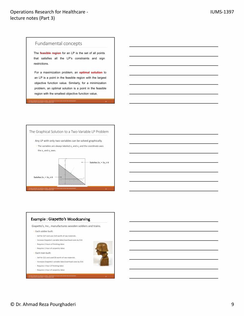
Fundamental concepts

25

The feasible region for an LP is the set of all points

that satisfies all the LP’s constraints and sign

restrictions.

For a maximization problem, an optimal solution to

an LP is a point in the feasible region with the largest

objective function value. Similarly, for a minimization

problem, an optimal solution is a point in the feasible

region with the smallest objective function value.


The Graphical Solution to a Two‐Variable LP Problem

Any LP with only two variables can be solved graphically.

◦ The variables are always labeled x1 and x2 and the coordinate axes

the x1 and x2 axes.

Satisfies 2x1 + 3x2 ≥ 6

Satisfies 2x1 + 3x2 ≤ 6 X1

1 2 3 4

1

2

3

4

X2

-1

-1


Giapetto’s, Inc., manufactures wooden soldiers and trains.

◦ Each soldier built:

◦ Sell for $27 and uses $10 worth of raw materials.

◦ Increase Giapetto’s variable labor/overhead costs by $14.

◦ Requires 2 hours of finishing labor.

◦ Requires 1 hour of carpentry labor.

◦ Each train built:

◦ Sell for $21 and used $9 worth of raw materials.

◦ Increases Giapetto’s variable labor/overhead costs by $10.

◦ Requires 1 hour of finishing labor.

◦ Requires 1 hour of carpentry labor.



IUMS‐1397


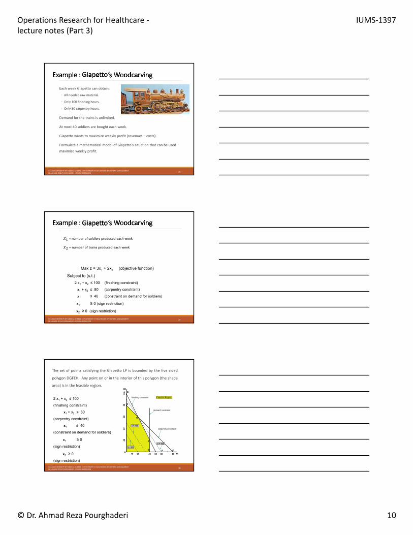
Each week Giapetto can obtain:

◦ All needed raw material.

◦ Only 100 finishing hours.

◦ Only 80 carpentry hours.

Demand for the trains is unlimited.

At most 40 soldiers are bought each week.

Giapetto wants to maximize weekly profit (revenues – costs).

Formulate a mathematical model of Giapetto’s situation that can be used

maximize weekly profit.


𝑥 = number of soldiers produced each week

𝑥 = number of trains produced each week

Max z = 3x1 + 2x2 (objective function)

Subject to (s.t.)

2 x1 + x2 ≤ 100 (finishing constraint)

x1 + x2 ≤ 80 (carpentry constraint)

x1 ≤ 40 (constraint on demand for soldiers)

x1 ≥ 0 (sign restriction)

x2 ≥ 0 (sign restriction)


The set of points satisfying the Giapetto LP is bounded by the five sided

polygon DGFEH. Any point on or in the interior of this polygon (the shade

area) is in the feasible region.

X1

X2

10 20 40 50 60 80

20

406

08

0100

finishing constraint

carpentry constraint

demand constraint

z = 60

z = 100

z = 180

Feasible Region

G

A

B

C

D

E

F

H

2 x1 + x2 ≤ 100

(finishing constraint)

x1 + x2 ≤ 80

(carpentry constraint)

x1 ≤ 40

(constraint on demand for soldiers)

x1 ≥ 0

(sign restriction)

x2 ≥ 0

(sign restriction)



IUMS‐1397


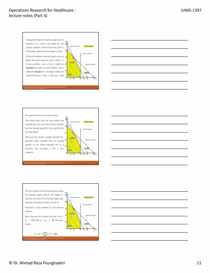
Having identified the feasible region for the

Giapetto LP, a search can begin for the

optimal solution which will be the point in

the feasible region with the largest z‐value.

To find the optimal solution, graph a line on

which the points have the same z‐value. In

a max problem, such a line is called an

isoprofit line while in a min problem, this is

called the isocost line. The figure shows the

isoprofit lines for z = 60, z = 100, and z = 180

X1

X2

10 20 40 50 60 80

2040

6080

100



demand constraint

z = 60

z = 100

z = 180

Feasible Region

G

A

B

C

D

E

F

H


All isoprofit lines have the same slope.

This means that once we have drawn one

isoprofit line, we can find all other isoprofit

lines by moving parallel to the isoprofit line

we have drawn.

After you have drawn a single isoprofit line,

generate other isoprofit lines by moving

parallel to the drawn isoprofit line in a

direction that increases z (for a max

problem).X1

X2

10 20 40 50 60 80

2040

6080

100



demand constraint

z = 60

z = 100

z = 180

Feasible Region

G

A

B

C

D

E

F

H


The last isoprofit line intersecting (touching)

the feasible region defines the largest z‐

value of any point in the feasible region and

indicates the optimal solution to the LP.

Therefore, in our example G is the optimal

solution.

Note that point G is where the lines 2 x1 +

x2 = 100 and x1 + x2 = 80 intersect.

Hence

X1

X2

10 20 40 50 60 80

2040

6080

100



demand constraint

z = 60

z = 100

z = 180

Feasible Region

G

A

B

C

D

E

F

H

𝑥∗ 𝐺 2060

𝑍∗ 180



IUMS‐1397


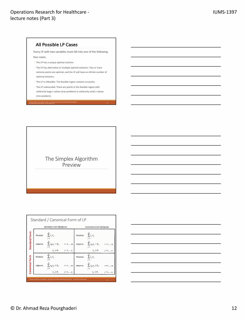
Every LP with two variables must fall into one of the following

four cases.

◦ The LP has a unique optimal solution.

◦ The LP has alternative or multiple optimal solutions: Two or more

extreme points are optimal, and the LP will have an infinite number of

optimal solutions.

◦ The LP is infeasible: The feasible region contains no points.

◦ The LP unbounded: There are points in the feasible region with

arbitrarily large z‐values (max problem) or arbitrarily small z‐values

(min problem).


The Simplex Algorithm Preview

Standard / Canonical Form of LP

ISFAHAN UNIVERSITY OF TECHNOLOGY ‐ INDUSTRIAL & SYSTEMS ENGINEERING DEPARTMENT AHMAD REZA POURGHADERI ‐POURGHADERI.COM

36


IUMS‐1397


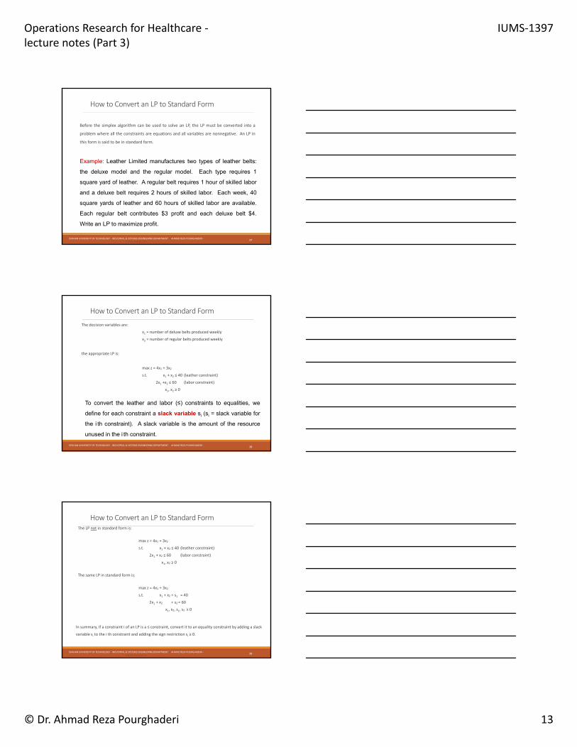
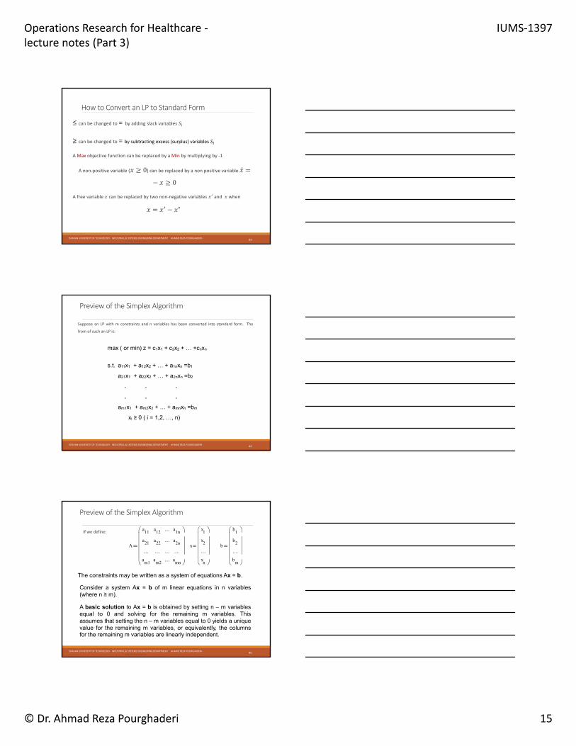
How to Convert an LP to Standard Form

Before the simplex algorithm can be used to solve an LP, the LP must be converted into a

problem where all the constraints are equations and all variables are nonnegative. An LP in

this form is said to be in standard form.

Example: Leather Limited manufactures two types of leather belts:

the deluxe model and the regular model. Each type requires 1

square yard of leather. A regular belt requires 1 hour of skilled labor

and a deluxe belt requires 2 hours of skilled labor. Each week, 40

square yards of leather and 60 hours of skilled labor are available.

Each regular belt contributes $3 profit and each deluxe belt $4.

Write an LP to maximize profit.


37

The decision variables are:

x1 = number of deluxe belts produced weekly

x2 = number of regular belts produced weekly

the appropriate LP is:

max z = 4x1 + 3x2

s.t. x1 + x2 ≤ 40 (leather constraint)

2x1 +x2 ≤ 60 (labor constraint)

x1, x2 ≥ 0

To convert the leather and labor (≤) constraints to equalities, we

define for each constraint a slack variable si (si = slack variable for

the i th constraint). A slack variable is the amount of the resource

unused in the i th constraint.



38

The LP not in standard form is:

max z = 4x1 + 3x2

s.t. x1 + x2 ≤ 40 (leather constraint)

2x1 + x2 ≤ 60 (labor constraint)

x1, x2 ≥ 0

The same LP in standard form is:

max z = 4x1 + 3x2

s.t. x1 + x2 + s1 = 40

2x1 + x2 + s2 = 60

x1, x2, s1, s2 ≥ 0

In summary, if a constraint i of an LP is a ≤ constraint, convert it to an equality constraint by adding a slack

variable si to the i th constraint and adding the sign restriction si ≥ 0.



39


IUMS‐1397


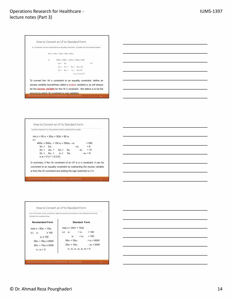
A ≥ constraint can be converted to an equality constraint. Consider the formulation below:

min z = 50 x1 + 20x2 + 30X2 + 80 x4

s.t. 400x1 + 200x2 + 150 x3 + 500x4 ≥ 500

3x1 + 2x2 ≥ 6

2x1 + 2x2 + 4x3 + 4x4 ≥ 10

2x1 + 4x2 + x3 + 5x4 ≥ 8

x1, x2, x3, x4 ≥ 0

To convert the i th ≥ constraint to an equality constraint, define an

excess variable (sometimes called a surplus variable) ei (ei will always

be the excess variable for the i th ≥ constraint. We define ei to be the

amount by which i th constraint is over satisfied.



40

Transforming the LP on the previous slide to standard form yields:

min z = 50 x1 + 20x2 + 30X2 + 80 x4

s.t.

400x1 + 200x2 + 150 x3 + 500x4 – e1 = 500

3x1 + 2x2 - e2 = 6

2x1 + 2x2 + 4x3 + 4x4 - e3 = 10

2x1 + 4x2 + x3 + 5x4 - e4 = 8

xi, ei > 0 (i = 1,2,3,4)

In summary, if the i th constraint of an LP is a ≥ constraint, it can be

converted to an equality constraint by subtracting the excess variable

ei from the i th constraint and adding the sign restriction ei ≥ 0.



41

If an LP has both ≤ and ≥ constraints, apply the previous procedures to the individual constraints.

Consider the example below.

max z = 20x1 + 15x2

s.t. x1 ≤ 100

x2 ≤ 100

50x1 + 35x2 ≤ 6000

20x1 + 15x2 ≥ 2000

x1, x2 > 0

max z = 20x1 + 15x2

s.t. x1 + s1 = 100

x2 + s2 = 100

50x1 + 35x2 + s3 = 6000

20x1 + 15x2 - e4 = 2000

x1, x2, s1, s2, s3, e4 > 0

Nonstandard Form Standard Form



42


IUMS‐1397


≤ can be changed to = by adding slack variables 𝑆

≥ can be changed to = by subtracting excess (surplus) variables 𝑆

A Max objective function can be replaced by a Min by multiplying by ‐1

A non‐positive variable (𝑥 0) can be replaced by a non positive variable �́�

𝑥 0

A free variable 𝑥 can be replaced by two non‐negative variables 𝑥 and 𝑥 when

𝑥 𝑥 𝑥"



43

Suppose an LP with m constraints and n variables has been converted into standard form. The

from of such an LP is:

max ( or min) z = c1x1 + c2x2 + … +cnxn

s.t. a11x1 + a12x2 + … + a1nxn =b1

a21x1 + a22x2 + … + a2nxn =b2

. . .

. . .

am1x1 + am2x2 + … + amnxn =bm

xi ≥ 0 ( i = 1,2, …, n)


44

Preview of the Simplex Algorithm

If we define:

The constraints may be written as a system of equations Ax = b.

A

a11

a21

....

am1

a12

a22

....

am2

....

....

....

....

a1n

a2n

....

amn

x

x1

x2

....

xn

b

b1

b2

....

bm

Consider a system Ax = b of m linear equations in n variables(where n ≥ m).

A basic solution to Ax = b is obtained by setting n – m variablesequal to 0 and solving for the remaining m variables. Thisassumes that setting the n – m variables equal to 0 yields a uniquevalue for the remaining m variables, or equivalently, the columnsfor the remaining m variables are linearly independent.


45



IUMS‐1397


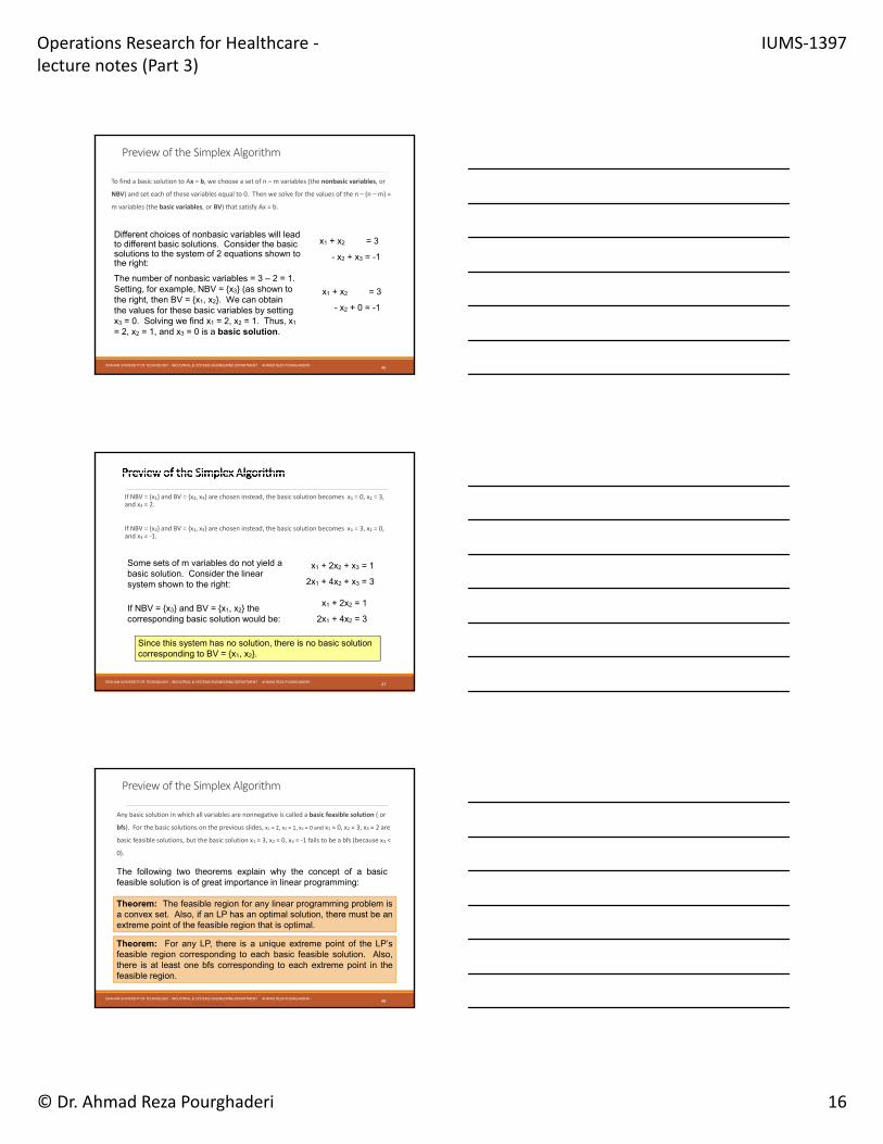
To find a basic solution to Ax = b, we choose a set of n – m variables (the nonbasic variables, or

NBV) and set each of these variables equal to 0. Then we solve for the values of the n – (n – m) =

m variables (the basic variables, or BV) that satisfy Ax = b.

x1 + x2 = 3

- x2 + x3 = -1

Different choices of nonbasic variables will lead to different basic solutions. Consider the basic solutions to the system of 2 equations shown to the right:

The number of nonbasic variables = 3 – 2 = 1. Setting, for example, NBV = {x3} (as shown to the right, then BV = {x1, x2}. We can obtain the values for these basic variables by setting x3 = 0. Solving we find x1 = 2, x2 = 1. Thus, x1

= 2, x2 = 1, and x3 = 0 is a basic solution.

x1 + x2 = 3

- x2 + 0 = -1


46


If NBV = {x1} and BV = {x2, x3} are chosen instead, the basic solution becomes x1 = 0, x2 = 3, and x3 = 2.

If NBV = {x2} and BV = {x1, x3} are chosen instead, the basic solution becomes x1 = 3, x2 = 0, and x3 = ‐1.

Some sets of m variables do not yield a basic solution. Consider the linear system shown to the right:

If NBV = {x3} and BV = {x1, x2} the corresponding basic solution would be:

x1 + 2x2 + x3 = 1

2x1 + 4x2 + x3 = 3

x1 + 2x2 = 1

2x1 + 4x2 = 3

Since this system has no solution, there is no basic solution corresponding to BV = {x1, x2}.


47


Any basic solution in which all variables are nonnegative is called a basic feasible solution ( or

bfs). For the basic solutions on the previous slides, x1 = 2, x2 = 1, x3 = 0 and x1 = 0, x2 = 3, x3 = 2 are

basic feasible solutions, but the basic solution x1 = 3, x2 = 0, x3 = ‐1 fails to be a bfs (because x3 <

0).

The following two theorems explain why the concept of a basicfeasible solution is of great importance in linear programming:

Theorem: The feasible region for any linear programming problem isa convex set. Also, if an LP has an optimal solution, there must be anextreme point of the feasible region that is optimal.

Theorem: For any LP, there is a unique extreme point of the LP’sfeasible region corresponding to each basic feasible solution. Also,there is at least one bfs corresponding to each extreme point in thefeasible region.


48


IUMS‐1397


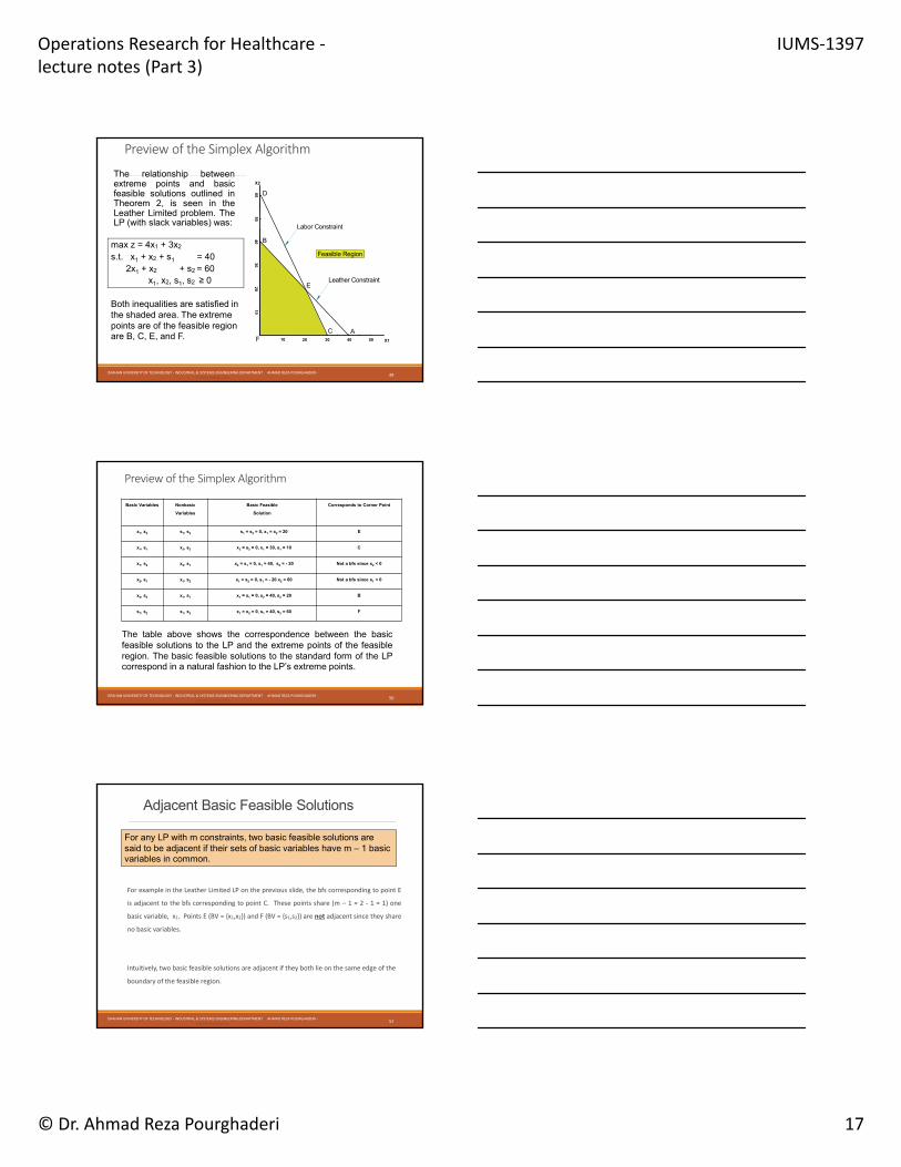
max z = 4x1 + 3x2

s.t. x1 + x2 + s1 = 402x1 + x2 + s2 = 60

x1, x2, s1, s2 ≥ 0

X1

X2

10 20 30 40

1020

3040

50

Feasible Region

50

60

E

ACF

B

D

Leather Constraint

Labor Constraint

Both inequalities are satisfied in the shaded area. The extreme points are of the feasible region are B, C, E, and F.

The relationship betweenextreme points and basicfeasible solutions outlined inTheorem 2, is seen in theLeather Limited problem. TheLP (with slack variables) was:


49


Basic Variables Nonbasic

Variables

Basic Feasible

Solution

Corresponds to Corner Point

x1, x2 s1, s2 s1 = s2 = 0, x1 = x2 = 20 E

x1, s1 x2, s2 x2 = s2 = 0, x1 = 30, s1 = 10 C

x1, s2 x2, s1 x2 = s1 = 0, x1 = 40, s2 = - 20 Not a bfs since s2 < 0

x2, s1 x1, s2 x1 = s2 = 0, s1 = - 20 x2 = 60 Not a bfs since s1 < 0

x2, s2 x1, s1 x1 = s1 = 0, x2 = 40, s2 = 20 B

s1, s2 x1, x2 x1 = x2 = 0, s1 = 40, s2 = 60 F

The table above shows the correspondence between the basicfeasible solutions to the LP and the extreme points of the feasibleregion. The basic feasible solutions to the standard form of the LPcorrespond in a natural fashion to the LP’s extreme points.


50


Adjacent Basic Feasible Solutions

For example in the Leather Limited LP on the previous slide, the bfs corresponding to point E

is adjacent to the bfs corresponding to point C. These points share (m – 1 = 2 ‐ 1 = 1) one

basic variable, x1. Points E (BV = {x1,x2}) and F (BV = {s1,s2}) are not adjacent since they share

no basic variables.

Intuitively, two basic feasible solutions are adjacent if they both lie on the same edge of the

boundary of the feasible region.

For any LP with m constraints, two basic feasible solutions are said to be adjacent if their sets of basic variables have m – 1 basic variables in common.


51


IUMS‐1397


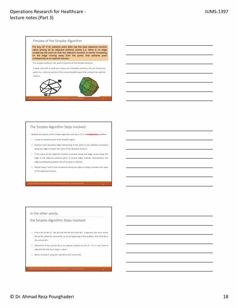
The simplex method is not used to examine all the feasible solutions.

It deals only with a small and unique set of feasible solutions, the set of extreme

points (i.e., extreme points) of the convex feasible space that contains the optimal

solution.


52


For any LP, if an extreme point (bfs) has the best objective functionvalue among all its adjacent extreme points (i.e. there is no edgecontaining the point so that the objective function is strictly increasingon the edge moving away from the point), that extreme pointcorresponds to an optimal solution.

The Simplex Algorithm Steps involved:

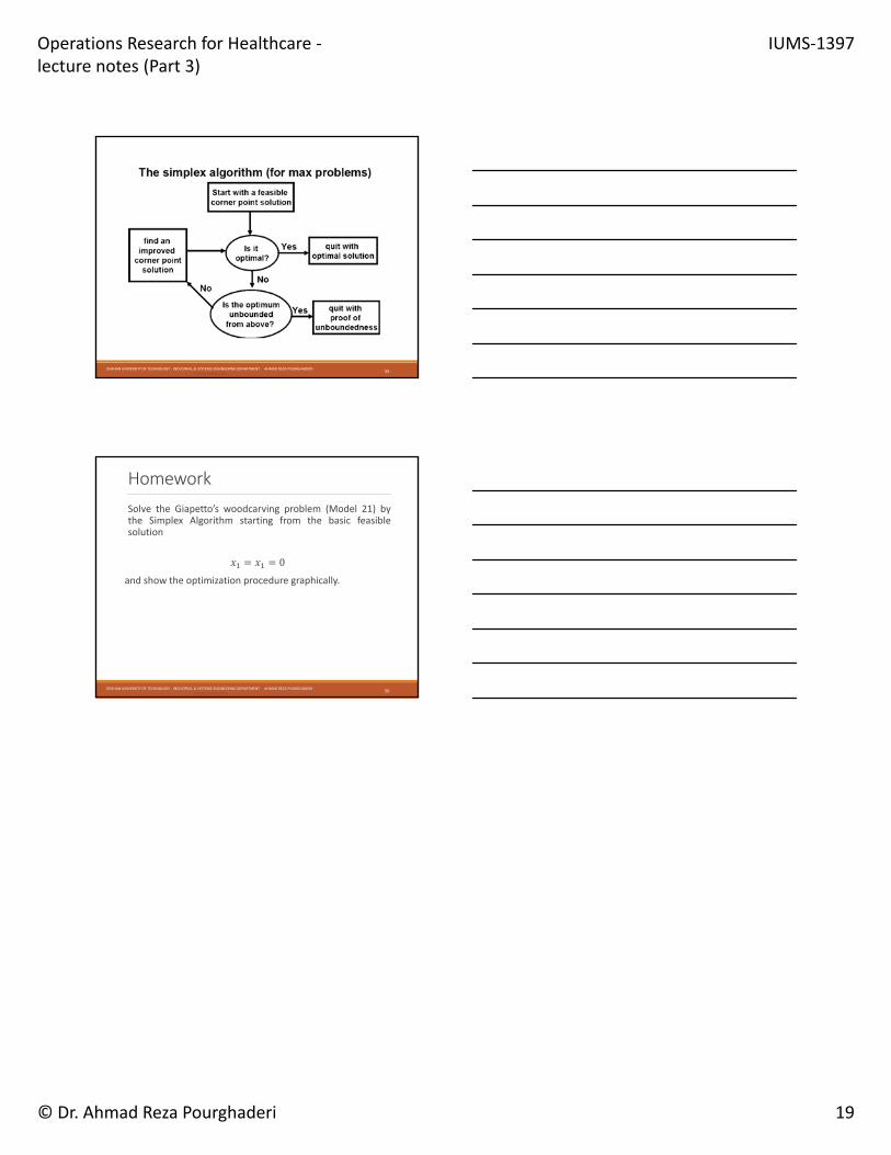
General description of the simplex algorithm solving an LP in a maximization problem:

1. Locate an extreme point of the feasible region.

2. Examine each boundary edge intersecting at this point to see whether movement

along any edge increases the value of the objective function.

3. If the value of the objective function increases along any edge, move along this

edge to the adjacent extreme point. If several edges indicate improvement, the

edge providing the greatest rate of increase is selected.

4. Repeat steps 2 and 3 until movement along any edge no longer increases the value

of the objective function.


53

1. Find a bfs to the LP. We will call this bfs the initial bfs. In general, the most recent

bfs will be called the current bfs, so at the beginning of the problem, the initial bfs is

the current bfs.

2. Determine if the current bfs is an optimal solution to the LP. If it is not, find an

adjacent bfs that has a larger z‐value.

3. Return to Step 2, using the new bfs as the current bfs.


54

In the other words,

the Simplex Algorithm Steps involved:


IUMS‐1397



55

Homework

Solve the Giapetto’s woodcarving problem (Model 21) bythe Simplex Algorithm starting from the basic feasiblesolution

𝑥 𝑥 0

and show the optimization procedure graphically.


56

Operations Research for Healthcare ‐ lecture notes (Part 3 ...

Documents