Operationally optimal vertex-based shape coding

Operationally Optimal Vertex-Based Shape CodingGuido M. Schuster3COM, Carrier Systems Business UnitAdvanced Technologies Research Center1800 W. Central Rd.Mount Prospect, Illinois 60056-2293Tel: (847) 222-2486Fax: (847) 222-0573E-mail: guido [email protected] Melnikov and Aggelos K. KatsaggelosNorthwestern UniversityDepartment of Electrical and Computer EngineeringMcCormick School of Engineering and Applied ScienceEvanston, Illinois 60208-3118Tel: (847) 491-7164Fax: (847) 491-4455E-mail: fgerrym,[email protected] this paper, we present a review of our work on rate-distortion based operationally optimal vertex-basedlossy shape encoding techniques. We approximate the boundary of a given shape by a low order curve, suchas a polygon, and consider the problem of �nding the approximation which leads to the smallest distortionfor a given number of bits. We also address the dual problem of �nding the approximation which leads tothe smallest bit rate for a given distortion. We consider two di�erent classes of distortion measures. The�rst class is based on the maximum operator (such as the maximum distance between a boundary and itsapproximation) and the second class is based on the summation operator (such as the total number of errorpels between a boundary and its approximation). For the �rst class, we derive a fast and operationallyoptimal scheme which is based on a shortest path algorithm for a weighted directed acyclic graph. For thesecond class, we propose a solution approach which is based on the Lagrange multiplier method, whichuses the above mentioned shortest path algorithm. Examples illustrate the e�ectiveness of the varioustechniques which are presented.

List of Figures1 Overview of the proposed approximation of an original boundary B by a polygon P. . . . . 292 Vector increments for the de�nition and ordering of the admissible control point set. Notethat vector vj starts at 0 and ends at j. . . . . . . . . . . . . . . . . . . . . . . . . . . . . . 303 Figures a, b, c, and d show the �nal result after the inner loop has been �nished for v1, v2,v3 and v4, for a maximum distance DM of one pel. The pels with a bold border indicate theoriginal boundary and the other pels are the admissible control points, where the numberof the associated boundary point is written inside it. . . . . . . . . . . . . . . . . . . . . . 314 The de�nition of a state for a polygon and a second order B-spline curve. Figure (a) showsthat for a polygon, knowing pk�1 makes the search for future control points independentfrom the control points already selected. Figure (b) shows that for a second order B-spline,knowing pk�2 and pk�1 makes the search for future control points independent from thecontrol points already selected. . . . . . . . . . . . . . . . . . . . . . . . . . . . . . . . . . . 325 A second degree B-spline curve with 8 curve segments Qk and a double control point at thebeginning of the curve. . . . . . . . . . . . . . . . . . . . . . . . . . . . . . . . . . . . . . . 336 Three di�erent ways for de�ning the segment distortion for a polygon-based approximationof the original boundary. Figure (a) shows the maximum distance, Figure (b) the error area,and Figure (c) the maximum distance band concept. . . . . . . . . . . . . . . . . . . . . . 347 Three di�erent ways for de�ning the segment distortion for a second order B-spline curve-based approximation of the original boundary. Figure (a) shows the maximum distance,Figure (b) the error area, and Figure (c) the maximum distance band concept. . . . . . . . 348 Interpretation of the boundary and the polygon approximation as a fully connected weighteddirected graph. Note that the set of all edges E equals f(ai; aj) 2 A2 : i 6= jg. Tworepresentative subsets are displayed: (a) f(a4; aj) 2 A2 : 8j 6= 4g and (b) f(a8; aj) 2 A2 :8j 6= 8g. . . . . . . . . . . . . . . . . . . . . . . . . . . . . . . . . . . . . . . . . . . . . . . 359 Each edge has a segment rate and a segment distortion associated with it. The edge weightis then a function (Ff�g) of these rates and distortion. For class one distortion measures,this function is di�erent than for class two distortion measures. . . . . . . . . . . . . . . . 3510 Examples of polygons with rapid changes in direction. . . . . . . . . . . . . . . . . . . . . . 36

11 Interpretation of the boundary and the polygon approximation as a weighted directed acyclicgraph. Note that the set of all edges E equals f(ai; aj) 2 A2 : i < jg. Two representativesubsets are displayed: (a) f(a4; aj) 2 A2 : 8j > 4g and (b) f(a8; aj) 2 A2 : 8j > 8g. . . . . . 3612 A simple DAG for a polygon approximation where A = B. The weights are de�ned as afunction of the segment rate and the segment distortion. . . . . . . . . . . . . . . . . . . . 3713 A simple DAG for a polygon approximation, where A � B. For this example we selectedA = fa0;0, a1;0; a1;1; a1;2; a2;0; a2;1; a2;2; a2;3; a3;0; a3;1; a4;0g. Furthermore, we only showthe edges originating in a1;i and terminating in a2;j , to keep the graph readable. Note thatthe edge (a1; a2) (for A = B) is replaced by the shown set of edges (a1;i; a2;j);8i; j. To �llthe entire graph with edges, this replacement is done for each edge in the original graph. . 3714 A simple DAG for a second order B-spline approximation, where A = B. We only labelthe �ve top edges with their respective weight function, but clearly, each edge has a weightfunction associated. . . . . . . . . . . . . . . . . . . . . . . . . . . . . . . . . . . . . . . . . 3815 The R�(Dmax) function, which is a non-increasing function exhibiting a staircase character-istic. The selected Rmax falls onto a discontinuity and therefore the optimal solution is ofthe form R�(D�max) < Rmax, instead of R�(D�max) = Rmax. . . . . . . . . . . . . . . . . . . 3916 A simple second order DPCM scheme is used to encode the control points. The angle �must take a value out of the following set: f�90;�45; 45; 90g. This is encoded with twobits. The length � is a number between 1 and 15 and is encoded using between 2 and 5 bits. 3917 Kid 2 in frame 17. Encoding using the maximum distortion measure. The distortion bandhas Dmax = 3. . . . . . . . . . . . . . . . . . . . . . . . . . . . . . . . . . . . . . . . . . . . . 4018 Average operational rate distortion curves for the �rst 100 frames of the "Kids" sequence. . 4119 The original � plane for the 17-th frame in the sequence. . . . . . . . . . . . . . . . . . . . 4220 The encoded � plane for the 17-th frame in the sequence using Dmax = 0:8. The algorithmrequired 858 bits resulting in a dn of 0.0257. . . . . . . . . . . . . . . . . . . . . . . . . . . 4321 Average operational rate distortion curves for the �rst 100 frames of the "Kids" sequence. . 4422 Kid 2 in frame 17. Encoding using the additive distortion measure. . . . . . . . . . . . . . . 4523 Average operational rate distortion curves for the �rst 100 frames of the "Kids" sequence. . 4624 The width of the control point band is inversely related to the con�dence in the location ofthe boundary pixels [27]. . . . . . . . . . . . . . . . . . . . . . . . . . . . . . . . . . . . . . 473

1 IntroductionMultimedia communications has become one of the fastest growing sectors of the communications industry.While the current drivers are primarily video streaming and video conferencing, a number of new applica-tions are in the horizon. Such applications, like multimedia libraries and interactive chat rooms, will needaccess to video data on an object by object basis, where video objects are de�ned by their shape, textureand motion.Current video coding standards, such as MPEG-1, MPEG-2, H.261, and H.263 are block-based codecs.The scene is divided into equal-sized square blocks for which the texture and motion are encoded. Noshape encoding is necessary, since the block size is known a priori. Unfortunately, a bit stream of such acoder does not lend itself to object based interaction with the data, since the shape of the objects (andtherefore the objects themselves) is not de�ned.Object based description of video is quite natural and there is a large amount of previous work. Forexample, most of the source material generated in a broadcast studio is based on the so-called chroma-keying technique, where an actor is �lmed in front of a blue screen and then moved in front of any desiredbackground. In [1] a second generation image coding scheme was formulated, where the segmentation ofthe image is transmitted explicitly. The underlying assumption is that the contours of regions are veryimportant for subjective image quality, whereas the texture of the regions is of lower importance. Object-based analysis-synthesis coding (OBASC) [2], which is a video coding paradigm, also follows the idea thatthe shape of moving objects is more important than the texture and that geometric distortions are lessnoticeable for a human observer than the coding artifacts of traditional block coders.Object based treatment of video sequences, necessitated by the emerging content driven applications,requires e�cient representation of object boundaries. The ultimate goal is to allocate an available bitbudget optimally among the video scene components (shape, texture, motion) and within each component.Here, we address the issue of operationally optimal shape encoding, which is a step in the direction ofglobally optimal resource allocation in the object-oriented video.As already mentioned, the current video standards do not have the capability of encoding the shapeof a video object. This is one of the aspects the upcoming MPEG-4 Visual standard will address [3, 4,5, 6]. For the �rst time an international standard will enable the transmission of arbitrarily shaped videoobjects (VO). For a review of the upcoming MPEG-4 shape coding standard and a comparison with the1

operationally optimal shape coding techniques discussed in this paper, the reader is referred to [7].It is common practice in computer graphics to de�ne the shape of an object using a so called � map,Mk, given by Mk = fmk(x; y)j0 � x � X; 0 � y � Y g; 0 � mk � 255: (1)This alpha map is of the same size as the frame, which is of dimension X � Y pels. It speci�es whether acertain pel is part of the visual object (VO) (mk(x; y) > 0) or not (mk(x; y) = 0), and whether the pel istransparent (mk(x; y) < 255) or opaque (mk(x; y) = 255). While in computer graphics transparent objectsare important, for the purpose of video description and coding, opaque objects are more common, andhence most shape coders are designed for opaque objects.There are two major classes of shape coders, bitmap based coders and contour based coders. Bitmapbased coders look at the � map as just another black and white (or gray scale) image which needs to beencoded e�ciently. One can argue that to some degree these coders break the object oriented paradigm.Bitmap-based shape coders are used in the very popular group 3 fax standard [8] and in the emergingbi-level standard JBIG [9] as well as in MPEG-4. The contour-based coders, on the other hand, try toencode the boundary of the object, by following its outline. The proposed operationally optimal techniquesbelong to this class of shape coders. In the following we provide a brief review of contour-based coders.Various bitmap-based and contour-based shape coders are discussed in detail in [7].One of the �rst contour coders was proposed by Freeman [10]. He suggested the use of chain codingfor boundary quantization and encoding, which has attracted considerable attention over the last thirtyyears [11, 12, 13, 14, 15]. The curve is quantized using the grid intersection scheme [10] and the quantizedcurve is represented using a string of increments. Since the planar curve is assumed to be continuous,the increments between grid points are limited to the 8 grid neighbors, and hence an increment can berepresented by 3 bits. For lossless encoding of boundary shapes, an average 1.2 bits/boundary pel and 1.4bits/boundary pel are required respectively for a 4 and an 8 neighbor grid [16]. There have been manyextensions to this basic scheme such as the generalized chain codes [11], where the coding e�ciency hasbeen improved with the use of links of di�erent length and di�erent angular resolution. In [14] a schemeis presented which utilizes patterns in a chain code string to increase the coding e�ciency, and in [15]di�erential chain codes are presented, which employ the statistical dependency between successive links.There has also been interest in the theoretical performance of chain codes. In [12] the performance of2

di�erent quantization schemes is compared, whereas in [13] the rate distortion characteristics of certainchain codes are studied. In this paper, we are not concerned with the quantization of the continuous curve,since we assume that the object boundaries are given with pel accuracy.A polygon-based shape representation was developed for OBASC [17, 18]. As a quality measure, theEuclidean distance Dmax between the original and the approximated contour was used. During subjectiveevaluations of CIF (352�288 pels) video sequences, it was found that allowing a peak distance ofD�max = 1:4pel is su�cient to allow proper representations of objects in low bitrate applications. Hence the lossypolygon approximation was developed. The polygon approximation is computed using the two contourpoints with the maximum distance between them as the starting point. Then, points are added to thepolygon where the approximation error between the polygon and the contour is the highest. This isrepeated until the shape approximation error is less than D�max. In a last step, splines are de�ned usingthe polygon points. If the spline approximation does not result in a larger approximation error betweentwo neighboring polygon points, the spline approximation is used. This leads to a smoother representationof the shape. Vertex coordinates and the curve type between two vertices are arithmetically encoded.Several other optimal, as well as, greedy non-optimal vertex-based curve approximation algorithms havebeen proposed in the literature. With a �xed number of approximating line segments and no restrictionon their connectivity, an optimal (with respect to distortion) segment placement problem was solved byBellman in [19]. In [20, 21] a fan-based approach, based on the concept of overlapping visibility regions,was used in which a greedy minimax strategy arrived at a polygonal approximation with a small numberof connected line segments and end-points on the original curve. The same problem was solved optimallyin [22] with the use of dynamic programming. The rate for encoding the vertices of the polygons was nottaken into account, therefore these approaches are not optimal in the rate-distortion sense. In [23] thisapproach was extended to allow the line end-points to be o� the original boundary and DPCM encodingof the control points was taken into account in the cost minimization process.In [24, 25] B-spline curves are used to approximate a boundary. An optimization procedure is formulatedfor �nding the optimal locations of the control points by minimizing the mean squared error between theboundary and the approximation. This is an appropriate procedure when the smoothing of the boundaryis the main objective. When, however, the encoding of the resulting control points is taken into account,the tradeo� between the encoding cost and the resulting distortion needs to be considered. By selectingthe mean squared error as the distortion measure and allowing for the location of the control points to be3

anywhere on the plane, the resulting optimization problem is continuous and convex and can be solvedeasily. In order to encode the positions of the resulting control points e�ciently, however, one needs toquantize them, and therefore the optimality of the solution is lost. It is well known that the optimalsolution to a discrete optimization problem (quantized locations) does not have to be close to the solutionof the corresponding continuous problem.The above methods for polygon/spline representation achieve good results but they cannot claim op-timality. In this paper we propose a framework for the operationally optimal contour encoding of objectboundaries in the intra mode. The techniques discussed here, even though dealing with still boundaryapproximations, are designed to be a part of a video codec. Hence, throughout the paper, we refer to videocoding as the target application, but we concentrate on the intra mode of operation and do not utilize thetemporal correlation between frames for shape prediction. While optimal shape coding techniques are ableto outperform existing shape coders, the proposed framework also allows for additional capabilities. Forexample, these techniques allow for the optimal bit allocation among objects in a scene and/or sequence[26], simple rate control, combination of automatic segmentation and compression [27], etc.The techniques presented in this paper for the operationally optimal boundary encoding can also beapplied to the near-lossless encoding of one-dimensional signals. An example is represented by the workin [28, 29], where ECG signals are compressed using a min-max approach. They can even be applied tothe near-lossless encoding of two-dimensional signals. In [23] a piecewise linear approximation was used byconverting an image into a 1-D signal with a zig-zag or a Hilbert scan. In this framework, a near-losslessimage compression problem is easily formulated using the minimum maximum criterion. This may bethe coding technique of choice for applications requiring a guaranteed accuracy of approximation at everypixel, as opposed to a global distortion measure, like the mean-squared error.The rest of the paper is organized as follows. In section 2 we de�ne the problem mathematically andintroduce the necessary notation. In section 3 we present the basic idea behind the proposed algorithms.In section 4 we discuss the constraints imposed on the code used to encode the approximation. In section5 we introduce a de�nition of distortion which �ts into the proposed framework. In section 6 we introducethe directed acyclic graph (DAG) formulation of the problem, which results in a fast solution approach.In section 7 we show how the DAG algorithm can be used to �nd the approximation with the minimummaximum segment distortion for a given rate. In section 8 we show how the DAG algorithm can be usedto �nd the approximation with the smallest total distortion for a given rate. In section 9 we present4

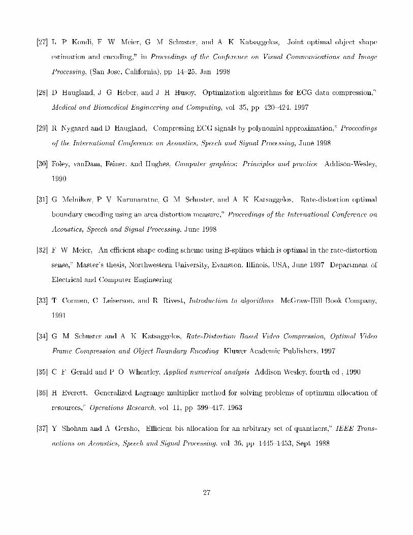
experimental results and in section 10 we conclude the paper and point out directions for future research.2 Problem FormulationIn this section we formulate the problem mathematically and introduce the necessary notation. For thepurpose of the discussion, we focus on the approximation of a given boundary by a polygon, as depictedin Fig. 1. We note here, that the proposed shape encoding techniques are not restricted to polygons. Infact they can be extended to any order curve. We use second order B-spline curves to illustrate this pointlater on. As can be seen in Fig. 1, there are three sets involved in the proposed framework. The boundaryset B, the control point set P and the admissible control point set A. While B is given, we are trying to�nd P , which must be a subset of A, such that the resulting approximation curve is as close as possible toB, (measured by a distortion measure, discussed in section 5), for a given bit rate necessary to encode P(using a code satisfying the constraints discussed in section 4).We use the notation shown in Fig. 1. We denote by B = fb0; : : : ; bNB�1g the connected boundarywhich is an ordered set, where bj is the j-th point of B and NB is the total number of points in B. Notethat in the case of a closed boundary, as shown in Fig. 1, b0 = bNB�1. We denote by P = fp0; : : : ; pNP�1gthe curve control points used to approximate B, which is also an ordered set. Note that for a polygon, pkis the k-th vertex of P and NP the total number of vertices in P . Since P is an ordered set, the orderingrule and the set of control points uniquely de�ne the approximation.Having established the above notation, operationally optimal shape coding can now be formalized asthe solution to the following discrete, constrained optimization problem:minp0;:::;pNP�1D(p0; : : : ; pNP�1); subject to: R(p0; : : : ; pNP�1) � Rmax; (2)where D(�) is the distortion measure, quantifying the error between the approximation and the original,R(�) is the bit rate required to encode the control points P , and Rmax is the maximum bit rate permittedfor the encoding of the boundary. We also present algorithms which solve the dual problem, that is,minp0;:::;pNP�1R(p0; : : : ; pNP�1); subject to: D(p0; : : : ; pNP�1) � Dmax; (3)where Dmax is the maximum distortion permitted. Note that there is an inherent tradeo� between the rateand the distortion in the sense that a small distortion requires a high rate, whereas a small rate results ina high distortion. As we will see the solution approaches for problems (2) and (3) are related in the sense5

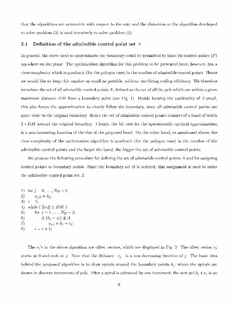
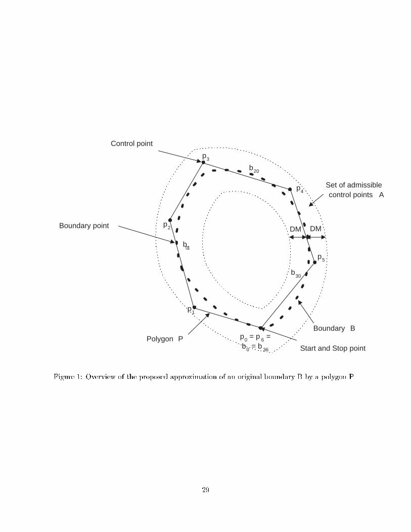
that the algorithms are symmetric with respect to the rate and the distortion or the algorithm developedto solve problem (3) is used iteratively to solve problem (2).2.1 De�nition of the admissible control point set AIn general, the curve used to approximate the boundary could be permitted to place its control points (P )anywhere on the plane. The optimization algorithm for this problem to be presented later, however, has atime complexity which is quadratic (for the polygon case) in the number of admissible control points. Hencewe would like to keep this number as small as possible, without sacri�cing coding e�ciency. We thereforeintroduce the set of all admissible control points A, de�ned as the set of all the pels which are within a givenmaximum distance DM from a boundary point (see Fig. 1). Beside keeping the cardinality of A small,this also forces the approximation to closely follow the boundary, since all admissible control points arequite close to the original boundary. Hence the set of admissible control points consists of a band of width2 � DM around the original boundary. Clearly, the bit rate for the operationally optimal approximationis a non-increasing function of the size of the proposed band. On the other hand, as mentioned above, thetime complexity of the optimization algorithm is quadratic (for the polygon case) in the number of theadmissible control points and the larger the band, the bigger the set of admissible control points.We propose the following procedure for de�ning the set of admissible control points A and for assigningcontrol points to boundary points. Since the boundary set B is ordered, this assignment is used to orderthe admissible control point set A.1) for j = 0; : : : ; NB � 1;2) aj;0 = bj ;3) i = 1;4) while ( jjvijj � DM )5) for j = 1; : : : ; NB � 2;6) if fbj + vig =2 A7) aj;i = bj + vi;8) i = i+ 1;The vi's in the above algorithm are o�set vectors, which are displayed in Fig. 2. The o�set vector vjstarts at 0 and ends at j. Note that the distance jjvj jj is a non-decreasing function of j. The basic ideabehind the proposed algorithm is to draw spirals around the boundary points bj, where the spirals aredrawn in discrete increments of pels. After a spiral is advanced by one increment, the new pel bj + vi is an6

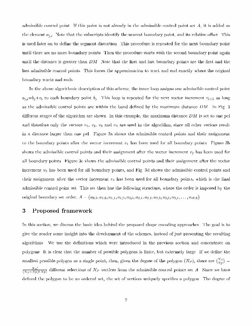
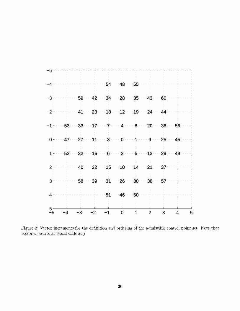
admissible control point. If this point is not already in the admissible control point set A, it is added asthe element aj;i. Note that the subscripts identify the nearest boundary point, and its relative o�set. Thisis used later on to de�ne the segment distortion. This procedure is repeated for the next boundary pointuntil there are no more boundary points. Then the procedure starts with the second boundary point againuntil the distance is greater than DM . Note that the �rst and last boundary points are the �rst and thelast admissible control points. This forces the approximation to start and end exactly where the originalboundary starts and ends.In the above algorithmic description of this scheme, the inner loop assigns one admissible control pointaj;i=bj+vi to each boundary point bj. This loop is repeated for the next vector increment vi+1 as longas the admissible control points are within the band de�ned by the maximum distance DM . In Fig. 3di�erent stages of the algorithm are shown. In this example, the maximum distance DM is set to one peland therefore only the vectors v1, v2, v3 and v4 are used in the algorithm, since all other vectors resultin a distance larger than one pel. Figure 3a shows the admissible control points and their assignmentto the boundary points after the vector increment v1 has been used for all boundary points. Figure 3bshows the admissible control points and their assignment after the vector increment v2 has been used forall boundary points. Figure 3c shows the admissible control points and their assignment after the vectorincrement v3 has been used for all boundary points, and Fig. 3d shows the admissible control points andtheir assignment after the vector increment v4 has been used for all boundary points, which is the �naladmissible control point set. This set then has the following structure, where the order is imposed by theoriginal boundary set order, A = fa0;0; a1;0; a1;1; a1;2; a2;0; a2;1; a2;2; a2;3; a3;0; a3;1; : : : ; a18;0g.3 Proposed frameworkIn this section, we discuss the basic idea behind the proposed shape encoding approaches. The goal is togive the reader some insight into the development of the schemes, instead of just presenting the resultingalgorithms. We use the de�nitions which were introduced in the previous section and concentrate onpolygons. It is clear that the number of possible polygons is �nite, but extremely large. If we de�ne thesmallest possible polygon as a single point, then, given the degree of the polygon (NP ), there are �NANP � =NA!(NA�NP )!�NP ! di�erent selections of NP vertices from the admissible control points set A. Since we havede�ned the polygon to be an ordered set, the set of vertices uniquely speci�es a polygon. The degree of7

the polygon (NP ) is also a variable, therefore the total number of possible polygons is equal toNAXk=1 NA!(NA � k)! � k! : (4)Clearly an exhaustive search is not a feasible approach and we need to look for a fast formulation of thesolution to the problem.The fast graph algorithm we introduce in section 6 is based on the following observation. If we �xthe current vertex of a polygon, then changing future vertices does not change the polygon up to andincluding the current vertex (see Figure 4a). In other words, knowing the position of the current vertex,makes the past independent of the future. Clearly, the knowledge of the current vertex represents a stateof this system. Therefore, given we have an optimal approximation for all the previous vertices, �nding theoptimal approximation for the current vertex simply requires the selection of the optimal approximationbetween all previous vertices and the current one.In the case of a polygonal approximation, the curve between two state values is simply a straight line, ascan be seen in Figure 4a. For higher order curves, such as a B-spline, the situation is a bit more complicated.Before continuing, it is worthwhile to present a review of B-splines. These are a family of parametric curveswhich have proven to be very useful in boundary encoding [7]. In the following discussion, we concentrateon second order B-splines. However, the presented theory can be generalized to higher order curves. Also,it should be noted that �rst order B-splines are equivalent to polygons.A B-spline is a speci�c curve type from the family of parametric curves [30]. A parametric curveconsists of one or more curve segments. Each curve segment is de�ned by (n+ 1) control points where nde�nes the degree of the curve. The control points are located around the curve segment and together witha constant base matrix M they solely de�ne the shape of the curve. A two dimensional curve segment Quwith control points (pu�1; pu; pu+1) is de�ned in the x� y plane as follows:Qu(pu�1; pu; pu+1; t) = h x(t); y(t) i ; for 0 � t � 1; and 0 otherwise. (5)The points at the beginning and the end of a curve segment are called knots and can be found by settingt = 0 and t = 1. The following is the de�nition for a second degree curve segment, with u the index for thedi�erent curve segments, and pu;x and pu;y, respectively, the horizontal and vertical coordinates of control8

point pu, Qu(pu�1; pu; pu+1; t) = T �M � P= h t2 t 1 i � 264 m1;1 m1;2 m1;3m2;1 m2;2 m2;3m3;1 m3;2 m3;3 375 � 264 pu�1;x pu�1;ypu;x pu;ypu+1;x pu+1;y 375 : (6)Both, the base matrixM , with speci�c constant parameters for each speci�c type of a parametric curve,and the control point matrix P , with (n+ 1) control points, de�ne the shape of Qu in a two dimensionalplane. Every point of the curve segment can be calculated with Eq. (6) by letting t vary from 0 to 1. Everycurve segment can be calculated independently in order to calculate the entire curve Q, consisting of NPcurve segments, which is of the following form,Q(t0) =PNPu=1Qu(pu�1; pu; pu+1; t0 � u+ 1); with 0 � t0 � NP + 1: (7)Among common parametric curves are the Bezier curve and the B-spline curve. For the presentation inthis paper we chose a second order (quadratic) uniform non-rational B-spline curve [30] with the followingbase matrix, M = 264 0:5 �1:0 0:5�1:0 1:0 0:00:5 0:5 0:0 375 : (8)Figure 5 shows such a second order B-spline curve. The shape coding method presented in this paper isindependent of the matrix M and degree n, that is, parametric curves of higher order can be used.The beginning and the end of the boundary approximation have to be treated as special cases, if the�rst curve segment should start exactly at the �rst boundary point and the last curve segment should endexactly at the last boundary point. When we use a double control point (such as pu�1 = pu) the curvesegment Qu will begin exactly at the double control point (see Figure 5). We apply this property to thebeginning and the end of the curve, so that p0 = p1 and pNP = pNP+1. These two special cases can easilybe incorporated into the boundary approximation algorithm.Recall the argument made for the polygon case, which is based on the fact that knowledge of thelocation of the current vertex, decouples the future from the past. A similar argument can be made forhigher order curves, such as the above introduced B-spline curves. Consider Fig. 4b which shows a secondorder B-spline curve. As mentioned above, three control points completely de�ne a curve segment. Hence ifwe know the last two control points, then the future is independent from the past. In other words, when thelast two control points are �xed, then the approximation up to and including these two control points doesnot change if future control points are changed. Clearly in a second order B-spline curve approximation,9

a state of the system contains the last two control points. In general, the order of the curve is equivalentto the dimensionality of the state space. As we will see later on, the dimensionality is in the exponent ofthe time complexity of the proposed algorithms, and hence it should be kept as small as possible.In summary, the basic idea behind the proposed algorithms is the fact that one can de�ne a state (ofsmall dimensionality) which makes the future of the optimization process independent from its past. Ourde�nition of the state varies according to the order of the curve used to generate approximating segments.Thus, for example, with a second-order B-spline approximation, a state consists of two consecutive controlpoints, along with cost information. Since dimensionality of the state space directly depends on the curveused for the approximation, we will carefully constrain the code used for encoding the control points, sothat the order of prediction in a DPCM scheme does not require knowledge of control points not in thestate. Hence the state space dimension does not expand due to encoding. With this formulation, we willbe able to write the total rate as a sum of the segment rates. A similar concept applies to the de�nition ofdistortion, which we will also select such that the state space does not expand. In other words, we will beable to write the distortion of the approximation as a function of segment distortions. Note the importanceof the segment concept. A segment is the curve unit between two consecutive state values. In the case ofa polygon, a segment is just an edge between two vertices (see the line with the two arrows in Fig. 4a). Inthe case of a second order B-spline curve, a segment is de�ned in Eq. 6, and drawn with arrows in Fig. 4b.We will de�ne the segment rate and the segment distortion in the next two sections.4 RateIn this section we discuss the constraints imposed on the code structure by the proposed framework. As wepointed out in the previous section, the order of the approximation curve requires a certain dimensionalityof the state space. In general, there is a one to one correspondence between the order of the curve and therequired state space dimension. Note that the smaller the state space, the faster the optimal solution canbe found.A straightforward way of encoding the control points P is with the use of a �xed length code for eachpoint. Clearly this is not very e�cient, since consecutive control points are correlated. This correlationsuggests the use of di�erential pulse code modulation (DPCM) encoding of the points. In other words,the current point is predicted, using previous points, and only the di�erence between the prediction andthe current point is encoded. Because of the correlation among neighboring control points, the prediction10

error will be small in general, and can be coded e�ciently using an entropy code. Assuming that the orderof the predictor is o, then the rate for encoding the k-th segment is denoted by r(pk�o; : : : ; pk). In otherwords, the rate for encoding the k-th segment is de�ned as the rate of encoding the k-th control point (seeFigure 4), which depends on the position of the last o control points, since those are used in the predictionof pk. Clearly for a �rst order prediction, the rate to encode segment k only depends on the current andprevious control points. Furthermore, for a second order prediction, the segment rate only depends onthe current, and the two previous control points. The total rate can now be written as the sum of theindividual segment rates, that is,R(p0; : : : ; pNP�1) = NP�1+oXk=0 r(pk�o; : : : ; pk); (9)where all control points pi; i < 0 are equal to p0, and all control points pj; j > NP � 1 are equal to pNP�1.This forces the higher order curves to start at p0 and stop at pNP�1. Note that the rate r(p�o; : : : ; p0) isthe rate used to encode the �rst point p0. Further note that it is already known at the receiver that thelast point is repeated o times. Hence the rates r(pk�o; : : : ; pk) for k > NP � 1 are zero.By using DPCM which is of the same order as the curve used for the approximation, the total ratein Eq. (9) and the curve share the same state. In other words, the same arguments on the independenceof the future of the past, given knowledge of the present, also applies to the above total rate expression.Again, we are able to write the total rate as a function of its segment rates, which allows us to de�ne acompact state, to be used for the formulation of a fast optimization algorithm.5 DistortionIn this section we discuss various ways for de�ning the distortion between the original boundary andits approximation. Ideally, the de�nition of distortion should correspond to the visual quality of theapproximation perceived by a human observer. Unfortunately, it is not well understood how a humanobserver judges the quality of a boundary approximation, especially within the framework of a video scene,with many di�erent objects moving at di�erent speeds in di�erent directions.Nevertheless, there are mathematical distortion measures which are very meaningful, such as the max-imum distance between the original boundary and the approximation and/or the total area between theoriginal boundary and the approximation [26]. Note that similar to the rate, we propose to express thetotal distortion as a function of the segment distortions. By doing so, we will be able to formulate the total11

distortion using the same state, used for the rate and the approximation curve. Before we can de�ne thetotal distortion, we need to de�ne the segment distortions. Again, the decomposition of the total distortioninto segment distortions is crucial for our ability to formulate a fast optimization procedure.Consider Figure 6, which shows three popular segment distortions for polygons. Figure (a) showsthe maximum segment distance between the original boundary and the polygon edge. Note that eachadmissible control point is associated with its nearest boundary point (pk with be and pk�1 with ba). Thiswas accomplished by the admissible control point set construction algorithm we introduced in section 2.1.Besides the fact that the maximum distance has perceptual relevance, it is also easy to calculate for apolygonal approximation [26]. Figure (6b) shows an area-based segment distortion measure. The area isde�ned by the boundary between ba and be, the line between be and pk, the polygon edge between pk andpk�1 and the line between pk�1 and ba. There are di�erent ways one can calculate this area, which areeither based on a continuous or a discrete model [31]. In the continuous case, the boundary is thoughtof as a polygon and hence the area can be found by computational geometry. Clearly, the boundary isdiscrete and usually the polygon edge is also quantized to pel accuracy when displayed, hence one cancount the pels of the error area and use this count as a distortion measure. This approach will lead to thesame distortion measure as the one used in MPEG-4 [7]. Figure (6c) shows a di�erent approach which isbased on the idea of a distortion band. Basically, we draw a band of a given maximum distortion aroundthe original boundary, and if an edge stays inside this band, then its maximum distortion is acceptable.From a computational point of view, this is a fast method of de�ning the segment (and ultimately thetotal) distortion, but special care needs to be taken (using a sliding window) so that no trivial solutionsare selected [32].While Figure 6 shows three di�erent segment distortion measures for a polygon approximation, Figure 7shows them for a second order B-spline approximation. Note that the de�nition of a segment is slightly morecomplicated for higher order curves, since the control points do not directly correspond to the beginningand end of the segment. In other words, we need to �nd the boundary points which correspond to thebeginning (t = 0) and end (t = 1) of the curve segment. For example, for t = 0, this can be accomplishedby testing each boundary point between ba and bc, and picking the one which is the closest to t = 0. Wename that boundary point bb. In a similar fashion, we �nd bd. Clearly, having de�ned the curve segmentand its associated boundary points, all three previous polygon segment distortion measures can be similarlyde�ned for higher order curves. Note that the area for a second order B-spline approximation is outlined12

as follows: The boundary between bb and bd, the line from bd to t = 1, the B-spline between t = 1 andt = 0 and the line between t = 0 and bb.Independently of which of the above segment distortion measures is selected, they all depend directly onthe order o of the selected curve approximation, i.e., d(pk�o; : : : ; pk). Clearly this was the goal of breakingthe approximation into segments for which we can de�ne a segment distortion. As mentioned above, wecan now use these segment distortions in two di�erent ways to calculate the total distortion.We will treat two di�erent classes of total distortion measures. The �rst class is based on the maximumoperator (or equivalently, on the minimum operator) and is of the following form,D(p0; : : : ; pNP�1) = maxk2[0;:::;NP�1+o] d(pk�o; : : : ; pk); (10)where d(p�o; : : : ; p0) is de�ned to be equal to zero. We will refer to all distortion measures based on theabove de�nition as class one distortion measures.The second class of distortion measures is based on the summation operator and is of the followingform, D(p0; : : : ; pNP�1+o) = NP�1+oXk=0 d(pk�o; : : : ; pk); (11)where again where d(p�o; : : : ; p0) is de�ned to be equal to zero. We will refer to all distortion measuresbased on the above de�nition as class two distortion measures.In the remainder of this paper we will show how both classes of distortion measures can be treated,using a directed acyclic graph formulation with a slightly di�erent de�nition of the graph weights.6 Directed acyclic graph (DAG) formulationIn this section we show how a directed acyclic graph (DAG) can be used to formulate the problem at hand.We �rst concentrate on the polygon approximation, where the set of admissible control points A is equalto the original boundary B, which implies that aj;0 = bj. Since the second subscript will always be zerofor A=B, we will drop it in the notation. In this special case, there is a simple, one-to-one correspondencebetween graph vertices and control points (polygon vertices) and between graph edges and polygon edges.Recall that for a polygon approximation, the state we selected consists of the last control point. Thenwe showed that DPCM encoding of the control points, using a �rst order predictor, shares the same stateas the polygon approximation. We then carefully de�ned the approximation distortion, such that it isperceptually relevant and uses that same state as the rate and the polygon. In this section we now use the13

fact that these three entities share the same state to show how the selection of the optimal polygon canbe formulated using a DAG. Having formulated the problem as a shortest path problem through a DAGallows for the use of a fast dynamic programming algorithm to �nd the operationally optimal solution.For the proposed DAG formulation, we need to start the search for an optimal approximation at a givencontrol point. If the boundary is not closed, clearly the �rst boundary point a0 = b0 has to be selectedas the �rst control point p0. For a closed boundary, there is freedom in selecting the �rst control point.Experiments have shown that the performance of the algorithm is insensitive to the selection of the �rstcontrol point, and hence, we always use the �rst boundary point (which is arbitrary) as the �rst controlpoint, even for a closed boundary.Besides �xing the �rst control point of the approximation, we also require that the last control pointpNP�1 be equal to the last point of the boundary aNA�1 = bNB�1. This leads to a closed approximation fora closed boundary. For a boundary which is not closed, this condition, together with the starting condition,makes sure that the approximation starts and ends at the same points as the boundary.The optimization problems stated in Eqs. (2) and (3) can be formulated as a shortest path problemin a weighted directed graph G = (V;E), where V is the set of graph vertices, which is equivalent tothe admissible control point set A, and E is the set of edges (see Fig. 8). As stated above, in thisexample A = B and hence V = B, since every boundary point can be a control point. The edges betweenthe vertices represent the line segments of the polygon. A directed edge is denoted by the ordered pair(u; v) 2 E which implies that the edge starts at vertex u and ends at vertex v. Since every combination ofdi�erent control points can represent a line segment of a valid polygon, the edge set E is de�ned as follows,E = f(ai; aj) 2 A2 : 8i 6= jg (see Fig. 8). A path of order K from vertex u to a vertex u0 is an ordered setfv0; : : : ; vKg such that u = v0, u0 = vK and (vk�1; vk) 2 E for k = 1; : : : ;K. The order of the path is thenumber of edges in the path. The length of a path is de�ned as follows,KXk=1w(vk�1; vk); (12)where w(u; v) : E ! R is a weight function, specifying the cost of traversing this edge from u to v.By de�ning this weight function in di�erent ways, we will be able to �nd the optimal approximation forclass one and class two distortion measures. In all cases, the directed edge (u; v) is associated with itssegment rate r(u; v) and its segment distortion d(u; v), as can be seen in Fig. 9. The weight w(u; v) isthen a function of the segment rate and the segment distortion. The classical algorithm for solving such14

a single-source shortest-path problem, where all the weights are non-negative, is Dijkstra's algorithm [33],which has time complexity O(jV j2 + jEj). This is a signi�cant reduction compared to the time complexityof the exhaustive search. Recall that we de�ned the control point set as an ordered set for reasons whichwill now become apparent. We can further simplify the algorithm by observing that we would not like theoptimal path to select an admissible control point aj as a control point when the last selected control pointwas ai, where i > j. For example, a polygon where successive vertices are not assigned to boundary pointsin increasing order can exhibit rapid direction changes even when the original boundary is quite smooth(see Fig. 10). Therefore we add the restriction that not every possible combination of (ai; aj) representsa valid edge but only the ones for which i < j. Hence the edge set E is rede�ned in the following way,E = f(ai; aj) 2 A2 : i < jg (see Fig. 11). This restriction results in the fact that a given control point setuniquely speci�es the polygon. We used this fact before to derive the number of possible polygons in anexhaustive search approach.By de�ning the edge set E in the above fashion, we achieve two goals simultaneously. First, theselected approximation has to follow the original boundary without rapid direction changes, and second,the resulting graph is a weighted directed acyclic graph (DAG). For a DAG, there exists an algorithm for�nding a single-source shortest-path which is even faster than Dijkstra's algorithm. Following the notationin [33], we call this the DAG-shortest-path algorithm. The time complexity for the DAG-shortest-pathalgorithm is �(jV j + jEj), which means that the asymptotic lower bound (jV j + jEj) is equal to theasymptotic upper bound O(jV j+ jEj). Recall that in general V equals A and hence we would like to keepthe set of admissible control points as small as possible, as discussed in section 2.1.We now introduce the DAG-shortest-path algorithm. Let C�(ai) represent the minimum cost to reachthe admissible control point ai, (which in this case is identical to the boundary point bi, since A = B),from the source vertex a0 via an approximation. Clearly C�(aNB�1) is the cost of the shortest path fromthe source vertex a0 to the sink vertex aNB�1. Let q(ai) be a back pointer which is used to rememberthe optimal path. Consider Fig. 12 which shows a simple DAG for a polygon approximation. To �nd theshortest path through this graph, (which selects the optimal control points) we use the algorithm below.1) C�(a0) = w(a�1; a0);2) for i = 1; : : : ; NA � 1;3) C�(ai) =1;4) for i = 0; : : : ; NA � 2;5) for j = i+ 1; : : : ; NA � 1;6) calculate segment distortion d(ai; aj); 15

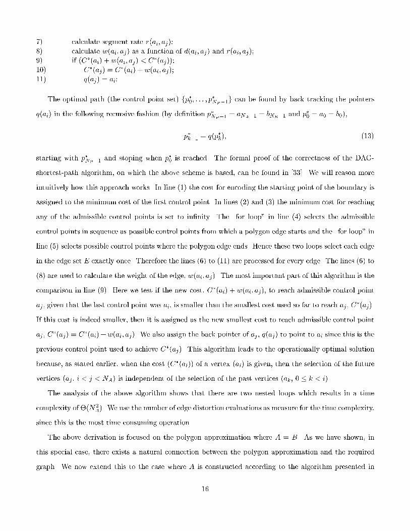
7) calculate segment rate r(ai; aj);8) calculate w(ai; aj) as a function of d(ai; aj) and r(ai; aj);9) if (C�(ai) + w(ai; aj) < C�(aj));10) C�(aj) = C�(ai) + w(ai; aj);11) q(aj) = ai;The optimal path (the control point set) fp�0; : : : ; p�NP�1g can be found by back tracking the pointersq(ai) in the following recursive fashion (by de�nition p�NP�1 = aNA�1 = bNB�1 and p�0 = a0 = b0),p�k�1 = q(p�k); (13)starting with p�NP�1 and stoping when p�0 is reached. The formal proof of the correctness of the DAG-shortest-path algorithm, on which the above scheme is based, can be found in [33]. We will reason moreintuitively how this approach works. In line (1) the cost for encoding the starting point of the boundary isassigned to the minimum cost of the �rst control point. In lines (2) and (3) the minimum cost for reachingany of the admissible control points is set to in�nity. The \for loop" in line (4) selects the admissiblecontrol points in sequence as possible control points from which a polygon edge starts and the \for loop" inline (5) selects possible control points where the polygon edge ends. Hence these two loops select each edgein the edge set E exactly once. Therefore the lines (6) to (11) are processed for every edge. The lines (6) to(8) are used to calculate the weight of the edge, w(ai; aj). The most important part of this algorithm is thecomparison in line (9). Here we test if the new cost, C�(ai) + w(ai; aj), to reach admissible control pointaj , given that the last control point was ai, is smaller than the smallest cost used so far to reach aj, C�(aj).If this cost is indeed smaller, then it is assigned as the new smallest cost to reach admissible control pointaj , C�(aj) = C�(ai) +w(ai; aj). We also assign the back pointer of aj, q(aj) to point to ai since this is theprevious control point used to achieve C�(aj). This algorithm leads to the operationally optimal solutionbecause, as stated earlier, when the cost (C�(ai)) of a vertex (ai) is given, then the selection of the futurevertices (aj , i < j < NA) is independent of the selection of the past vertices (ak, 0 � k < i).The analysis of the above algorithm shows that there are two nested loops which results in a timecomplexity of �(N2A). We use the number of edge distortion evaluations as measure for the time complexity,since this is the most time consuming operation.The above derivation is focused on the polygon approximation where A = B. As we have shown, inthis special case, there exists a natural connection between the polygon approximation and the requiredgraph. We now extend this to the case where A is constructed according to the algorithm presented in16

section 2.1. Basically the same graph (see Fig. 12) can be used, but we need to extend the vertices ofthe graph to include all the admissible control points which are associated with the same boundary point,i.e., aj is replaced by the set faj;0; aj;1; aj;2; : : :g. The extended graph is displayed in Fig. 13, where a0and a4 were not extended since they are the source and sink vertices, equivalent to the beginning and endof the original boundary. In Fig. 13, we only show the edges originating in a1;i and terminating in a2; j,to keep the graph readable. Note that the edge (a1; a2) in Fig. 12 is replaced by the shown set of edges(a1;i; a2;j); 8i; j. To �ll the entire graph with edges, this replacement is done for each edge in the originalgraph in Fig. 12.The next extension of the above algorithm is for higher order curves. Recall that we de�ned the orderof the curve to be equal to the order of prediction o and we are using a second order B-spline as an exampleof a higher order curve. As discussed in section 3, the state of an order o curve includes the last o controlpoints. We then showed that the same state can be used for encoding these control points with an order oDPCM scheme. We proposed to de�ne the total distortion as a function of segment distortions, such thatthe total distortion measure shares again the same state. We now discuss for a second order curve how theDAG needs to be changed to be able to �nd the optimal solution. To simplify the graph, we again assume A= B, and after we develop this graph it can be extended to include A � B, as was done above. As pointedout, the state consists the knowledge of the last two admissible control points (pk�2 = ai; pk�1 = aj),j > i,and hence all feasible values this state can take on are the vertices in the graph shown in Fig. 14. Theedges between the vertices then represent a segment of the curve, for which we have de�ned a segmentrate (r(pk�2; pk�1; pk)) and a segment distortion (d(pk�2; pk�1; pk)). These edges are than labeled withan edge weight (w(pk�2; pk�1; pk)), (for clarity reasons, in Fig. 14, we only labeled �ve edges with theirrespective weight, but clearly, each edge has a weight associated with it) which is a function of the segmentdistortion and the segment rate. In the next section, we will discuss how to select the function so thatthe DAG shortest path algorithm can be used to �nd the optimal approximation for distortion measuresof both classes. Note the di�erence in connectivity in Figs. 12 and 14. In Fig. 12, each vertex has an edgefor each future vertex, while in Fig. 14, each vertex has an edge for each future vertex, sharing the middlecontrol point. In other words, two consecutive vertices de�ne three control points, which in turn is enoughto de�ne a segment for a second order curve. The rate and distortion of this segment is then assigned tothe edge between the two vertices. Again, the DAG-shortest-path algorithm is used to �nd the optimalapproximation, where for this example the order of the state is two, which results in a time complexity17

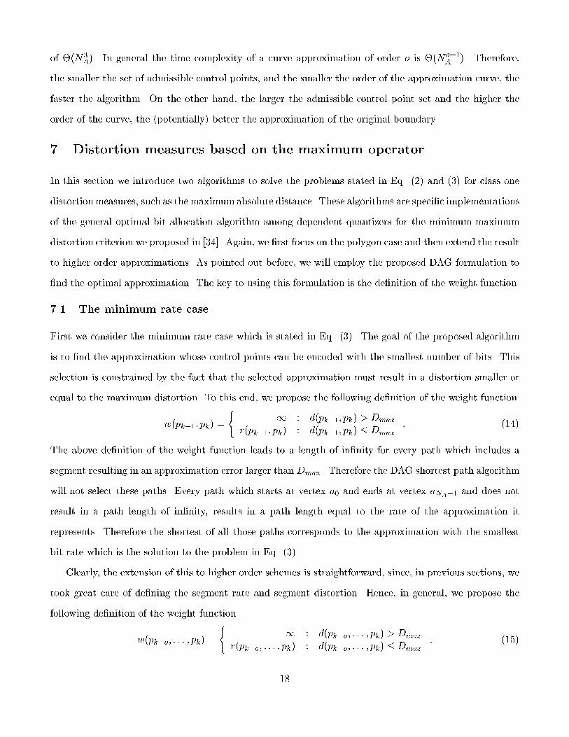
of �(N3A). In general the time complexity of a curve approximation of order o is �(No+1A ). Therefore,the smaller the set of admissible control points, and the smaller the order of the approximation curve, thefaster the algorithm. On the other hand, the larger the admissible control point set and the higher theorder of the curve, the (potentially) better the approximation of the original boundary.7 Distortion measures based on the maximum operatorIn this section we introduce two algorithms to solve the problems stated in Eq. (2) and (3) for class onedistortion measures, such as the maximum absolute distance. These algorithms are speci�c implementationsof the general optimal bit allocation algorithm among dependent quantizers for the minimum maximumdistortion criterion we proposed in [34]. Again, we �rst focus on the polygon case and then extend the resultto higher order approximations. As pointed out before, we will employ the proposed DAG formulation to�nd the optimal approximation. The key to using this formulation is the de�nition of the weight function.7.1 The minimum rate caseFirst we consider the minimum rate case which is stated in Eq. (3). The goal of the proposed algorithmis to �nd the approximation whose control points can be encoded with the smallest number of bits. Thisselection is constrained by the fact that the selected approximation must result in a distortion smaller orequal to the maximum distortion. To this end, we propose the following de�nition of the weight functionw(pk�1; pk) = ( 1 : d(pk�1; pk) > Dmaxr(pk�1; pk) : d(pk�1; pk) � Dmax : (14)The above de�nition of the weight function leads to a length of in�nity for every path which includes asegment resulting in an approximation error larger than Dmax. Therefore the DAG shortest path algorithmwill not select these paths. Every path which starts at vertex a0 and ends at vertex aNA�1 and does notresult in a path length of in�nity, results in a path length equal to the rate of the approximation itrepresents. Therefore the shortest of all those paths corresponds to the approximation with the smallestbit rate which is the solution to the problem in Eq. (3).Clearly, the extension of this to higher order schemes is straightforward, since, in previous sections, wetook great care of de�ning the segment rate and segment distortion. Hence, in general, we propose thefollowing de�nition of the weight functionw(pk�o; : : : ; pk) = ( 1 : d(pk�o; : : : ; pk) > Dmaxr(pk�o; : : : ; pk) : d(pk�o; : : : ; pk) � Dmax : (15)18

7.2 The minimum distortion caseWe now consider the minimum distortion case which is stated in Eq. (2). The goal of the proposedalgorithm is to �nd the approximation with the smallest distortion for a given bit budget for encodingits control points. Sometimes this is also called a rate constrained approach. Recall that for class onedistortion measures the total distortion is de�ned as the maximum of the segment distortions. Hence inthis section we propose an e�cient algorithm which �nds the approximation with the smallest maximumdistortion for a given bit rate.We propose an iterative solution to this problem which is based on the fact that we can solve the dualproblem stated in Eq. (3) optimally. Consider Dmax in Eq. (3) to be a variable. We derived in section 7.1an algorithm which �nds the polygonal approximation which results in the minimum rate for any Dmax.We denote this optimal rate by R�(Dmax). We proved in [34, 26] that the rate R�(Dmax) is a non-increasingfunction of Dmax, which means that D1max < D2max implies R�(D1max) � R�(D2max).Since the R�(Dmax) is a non-increasing function, we can use bisection [35] to �nd the optimal D�maxsuch that R�(D�max) = Rmax. Since this is a discrete optimization problem, the function R�(Dmax) is notcontinuous and exhibits a staircase characteristic (see Fig. 15). This implies that there might not exist aD�max such that R�(D�max) = Rmax. In this case the proposed algorithm will still �nd the optimal solution,which is of the form R�(D�max) < Rmax, but only after an in�nite number of iterations. Therefore if aDmax such that R�(Dmax) = Rmax is not found after a given maximum number of iterations, the algorithmis terminated. In this case, due to the discrete nature of optimization, after a number of iterations furtherbisecting the range of Dmax does not lead to corresponding re�nements in the vaues of R�(Dmax), inwhich case the algorithm terminates. It also terminates as soon as Rmax is approximated within speci�edaccuracy.Clearly, the time complexity of this approach for a �xed D�max is the same as for the DAG shortestpath algorithm. The shortest path algorithm is invoked several times by the bisection algorithm to �ndan D�max which results in R�(D�max) = Rmax. Hence the total time complexity is a linear function of thenumber of required iterations.19

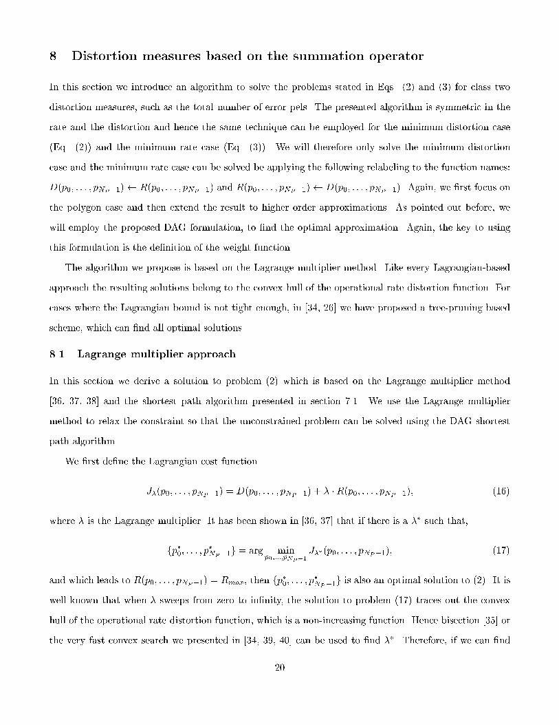
8 Distortion measures based on the summation operatorIn this section we introduce an algorithm to solve the problems stated in Eqs. (2) and (3) for class twodistortion measures, such as the total number of error pels. The presented algorithm is symmetric in therate and the distortion and hence the same technique can be employed for the minimum distortion case(Eq. (2)) and the minimum rate case (Eq. (3)). We will therefore only solve the minimum distortioncase and the minimum rate case can be solved be applying the following relabeling to the function names:D(p0; : : : ; pNP�1) R(p0; : : : ; pNP�1) and R(p0; : : : ; pNP�1) D(p0; : : : ; pNP�1). Again, we �rst focus onthe polygon case and then extend the result to higher order approximations. As pointed out before, wewill employ the proposed DAG formulation, to �nd the optimal approximation. Again, the key to usingthis formulation is the de�nition of the weight function.The algorithm we propose is based on the Lagrange multiplier method. Like every Lagrangian-basedapproach the resulting solutions belong to the convex hull of the operational rate distortion function. Forcases where the Lagrangian bound is not tight enough, in [34, 26] we have proposed a tree-pruning basedscheme, which can �nd all optimal solutions.8.1 Lagrange multiplier approachIn this section we derive a solution to problem (2) which is based on the Lagrange multiplier method[36, 37, 38] and the shortest path algorithm presented in section 7.1. We use the Lagrange multipliermethod to relax the constraint so that the unconstrained problem can be solved using the DAG shortestpath algorithm.We �rst de�ne the Lagrangian cost functionJ�(p0; : : : ; pNP�1) = D(p0; : : : ; pNP�1) + � �R(p0; : : : ; pNP�1); (16)where � is the Lagrange multiplier. It has been shown in [36, 37] that if there is a �� such that,fp�0; : : : ; p�NP�1g = arg minp0;:::;pNP�1 J��(p0; : : : ; pNP�1); (17)and which leads to R(p0; : : : ; pNP�1) = Rmax, then fp�0; : : : ; p�NP�1g is also an optimal solution to (2). It iswell known that when � sweeps from zero to in�nity, the solution to problem (17) traces out the convexhull of the operational rate distortion function, which is a non-increasing function. Hence bisection [35] orthe very fast convex search we presented in [34, 39, 40] can be used to �nd ��. Therefore, if we can �nd20

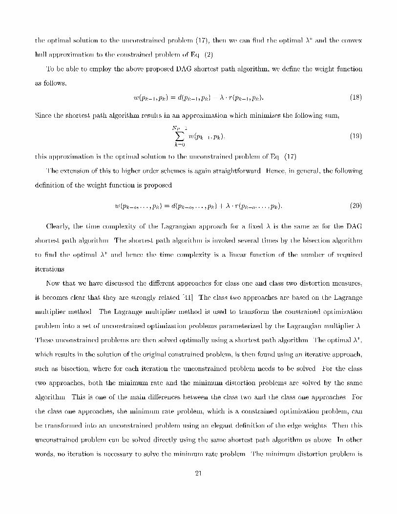
the optimal solution to the unconstrained problem (17), then we can �nd the optimal �� and the convexhull approximation to the constrained problem of Eq. (2).To be able to employ the above proposed DAG shortest path algorithm, we de�ne the weight functionas follows, w(pk�1; pk) = d(pk�1; pk) + � � r(pk�1; pk): (18)Since the shortest path algorithm results in an approximation which minimizes the following sum,NP�1Xk=0 w(pk�1; pk); (19)this approximation is the optimal solution to the unconstrained problem of Eq. (17).The extension of this to higher order schemes is again straightforward. Hence, in general, the followingde�nition of the weight function is proposedw(pk�o; : : : ; pk) = d(pk�o; : : : ; pk) + � � r(pk�o; : : : ; pk): (20)Clearly, the time complexity of the Lagrangian approach for a �xed � is the same as for the DAGshortest path algorithm. The shortest path algorithm is invoked several times by the bisection algorithmto �nd the optimal �� and hence the time complexity is a linear function of the number of requirediterations.Now that we have discussed the di�erent approaches for class one and class two distortion measures,it becomes clear that they are strongly related [41]. The class two approaches are based on the Lagrangemultiplier method. The Lagrange multiplier method is used to transform the constrained optimizationproblem into a set of unconstrained optimization problems parameterized by the Lagrangian multiplier �.These unconstrained problems are then solved optimally using a shortest path algorithm. The optimal ��,which results in the solution of the original constrained problem, is then found using an iterative approach,such as bisection, where for each iteration the unconstrained problem needs to be solved. For the classtwo approaches, both the minimum rate and the minimum distortion problems are solved by the samealgorithm. This is one of the main di�erences between the class two and the class one approaches. Forthe class one approaches, the minimum rate problem, which is a constrained optimization problem, canbe transformed into an unconstrained problem using an elegant de�nition of the edge weights. Then thisunconstrained problem can be solved directly using the same shortest path algorithm as above. In otherwords, no iteration is necessary to solve the minimum rate problem. The minimum distortion problem is21

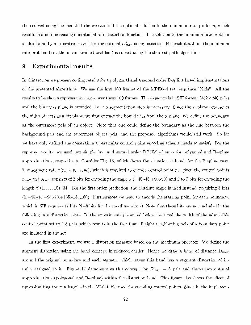
then solved using the fact that the we can �nd the optimal solution to the minimum rate problem, whichresults in a non-increasing operational rate distortion function. The solution to the minimum rate problemis also found by an iterative search for the optimal D�max using bisection. For each iteration, the minimumrate problem (i.e., the unconstrained problem) is solved using the shortest path algorithm.9 Experimental resultsIn this section we present coding results for a polygonal and a second order B-spline based implementationsof the presented algorithms. We use the �rst 100 frames of the MPEG-4 test sequence "Kids". All theresults to be shown represent averages over these 100 frames. The sequence is in SIF format (352�240 pels)and the binary � plane is provided, i.e., no segmentation step is necessary. Since the � plane representsthe video objects as a bit plane, we �rst extract the boundaries from the � plane. We de�ne the boundaryas the outermost pels of an object. Note that one could de�ne the boundary as the line between thebackground pels and the outermost object pels, and the proposed algorithms would still work. So farwe have only de�ned the constraints a particular control point encoding scheme needs to satisfy. For thereported results, we used two simple �rst and second order DPCM schemes for polygonal and B-splineapproximations, respectively. Consider Fig. 16, which shows the situation at hand, for the B-spline case.The segment rate r(pk�2; pk�1; pk), which is required to encode control point pk, given the control pointspk�2 and pk�3, consists of 2 bits for encoding the angle � (+45,-45,+90,-90) and 2 to 5 bits for encoding thelength � (1; : : : ; 15) [34]. For the �rst order prediction, the absolute angle is used instead, requiring 3 bits(0,+45,-45,+90,-90,+135,-135,180). Furthermore we need to encode the starting point for each boundary,which in SIF requires 17 bits (9+8 bits for the two dimensions). Note that these bits are not included in thefollowing rate distortion plots. In the experiments presented below, we �xed the width of the admissiblecontrol point set to 1.5 pels, which results in the fact that all eight neighboring pels of a boundary pointare included in the set.In the �rst experiment, we use a distortion measure based on the maximum operator. We de�ne thesegment distortion using the band concept introduced earlier. Hence we draw a band of distance Dmaxaround the original boundary and each segment which leaves this band has a segment distortion of in-�nity assigned to it. Figure 17 demonstrates this concept for Dmax = 3 pels and shows two optimalapproximations (polygonal and B-spline) within the distortion band. This �gure also shows the e�ect ofupper-limiting the run lengths in the VLC table used for encoding control points. Since in the implemen-22

tation only runs up to 15 are allowed, with some run lengths smaller than 15 also excluded, some longstraight line approximations were composed of consecutive runs of 15 along the same direction. We thenuse the above proposed DAG algorithm to �nd the set of control points which results in the smallest bitrate for this given maximum distortion Dmax. We do this for di�erent Dmax = 0.8, 1, 1.5, 2, 2.5 and 3pels. The resulting averaged operational rate distortion curves are displayed in Fig. 18 for polygonal andB-spline approximations. For comparison purposes, we also show in Fig. 18 the averaged operational ratedistortion curve for the case when the set of admissible control points A is equal to the set of the originalboundary points B (2 marks). Clearly choosing a wider admissible control point band leads to betterperformance in the operational rate distortion sense. Note that we �nd the optimal polygonal and secondorder B-spline approximations such that the rate required to encode the control points is minimized fora given maximum distortion Dmax. While the employed maximum distortion measure is a very usefulobjective criterion, we also display a single � plane for visual inspection. Figure 19 shows the original �plane for the 17-th frame and Fig. 20 shows the same plane after encoding and decoding, using a Dmax of0:8. The required bit rate is 858 bits and the resulting dn is 0.0257.In the second experiment, we use a distortion measure which is based on the summation operator. Tocreate the resulting averaged operational rate distortion curves, shown in Fig. 21, we swept the Lagrangianmultiplier � from zero to in�nity in discrete steps. For each � we encoded each frame in the sequence andeach boundary in each frame. We then recorded the resulting average rate and distortion (the average iswith respect to the 100 frames). Therefore the resulting bit allocation is optimal among all objects and allframes. Figure 22 shows the resulting polygonal and B-spline approximations when this distortion measurewas employed.Finally in Fig. 23 we combine all the results from the previous two experiments, using the dn distortionmetric. The reason for doing this is that dn is the metric used by MPEG-4 for evaluating the various shapeencoding techniques. As expected, each minimum summation technique outperforms its correspondingminimum maximum one. In addition, in Fig. 23, a result is shown (line with �) obtained using a di�erentVLC table than the one used in the rest of the curves. This was done to point to the potential bene�ts ofusing more e�cient VLCs.23

10 Summary and Future DirectionsIn this paper we proposed a framework for the rate distortion operationally optimal encoding of shapeinformation in the intra mode. We have shown that each curve approximation has a natural order. If thecontrol point encoding scheme is matched to this order and the distortion is carefully de�ned, then theoptimal approximation can be found using a directed acyclic graph (DAG) shortest path algorithm. Wehave shown that the minimummaximum distortion optimization problem and the minimum total (average)distortion optimization problem can both be solved by similar means, using an appropriate de�nition ofthe DAG weight function.The proposed framework is very powerful, in that it can be extended to solve various formulations ofthe shape coding problem also optimally. For example, in [26] we have shown in detail that the jointlyoptimal encoding of several shapes is a direct extension of the work presented here. In fact we haveused this optimal encoding of several shapes in the second experiment reported above (minimum averagedistortion). While we have shown �xed order optimization in this paper, a meaningful extension of thiswork is in the direction of mixed order approximations. Additional work has been done in including theso called lexicographic [42] optimality criterion in the minimum maximum distortion optimization. Thiscan be achieved easily in the proposed framework. The extension of the methodology used here to �nd theoperationally optimal shape approximations in the intra mode to the inter mode is a promising directionof future work and is currently under investigation. In [27] we have extended the shape encoding schemeto include the segmentation algorithm. In other words, we jointly �nd and encode optimally the shape ofa given object. Figure 24 illustrates how a variable-width admissible control point band is used for thatpurpose. While the proposed algorithms are already able to outperform any other lossy intra-mode shapeencoding scheme in the rate distortion sense, these schemes can still improve signi�cantly. We are currentlyfocusing on the control point encoding scheme, which is a very simple DPCM scheme. We expect thatother optimized schemes will result in further performance gains [43].References[1] M. Kunt, \Second-generation image coding techniques," Proceedings of the IEEE, vol. 73, pp. 549{574,Apr. 1985.[2] H. Musmann, M. H�otter, and J. Ostermann, \Object-oriented analysis-synthesis coding of moving24

images," Signal Processing: Image Communication, vol. 1, pp. 117{138, Oct. 1989.[3] L. Chiariglione, \MPEG and multimedia communications," IEEE Transactions on Circuits and Sys-tems for Video Technology, vol. 7, pp. 5{18, Feb 1997.[4] T. Sikora, \The MPEG-4 video standard veri�cation model," IEEE Transactions on Circuits andSystems for Video Technology, vol. 7, pp. 19{31, Feb 1997.[5] J. Ostermann and A. Puri, \Natural and synthetic video in MPEG-4," in Proceedings of the Interna-tional Conference on Acoustics, Speech and Signal Processing, May 1998.[6] R. Sch�afer and T. Sikora, \Digital video coding standards and their role in video communications,"Proceedings of the IEEE, vol. 38, pp. 907{924, June 1995.[7] A. K. Katsaggelos, L. P. Kondi, F. W. Meier, J. Ostermann, and G. M. Schuster, \MPEG-4 andrate-distortion-based shape-coding techniques," Proceedings of the IEEE, special issue on MultimediaSignal Processing, vol. 86, no. 6, pp. 1126{1154, June, 1998.[8] ITU-T, Telecommunication standardization sector of ITU, T.4, Standardization of group 3 facsimileterminals for document transmission.[9] ITU-T, Telecommunication standardization sector of ITU, T.82, Information technology, coded repre-sentation of picture and audio information, progressive bi-level image compression.[10] H. Freeman, \On the encoding of arbitrary geometric con�gurations," IRE Trans. Electron. Comput.,vol. EC-10, pp. 260{268, June 1961.[11] J. Saghri and H. Freeman, \Analysis of the precision of generalized chain codes for the representationof planar curves," IEEE Transactions on Pattern Analysis and Machine Intelligence, vol. PAMI-3,pp. 533{539, Sept. 1981.[12] J. Koplowitz, \On the performance of chain codes for quantization of line drawings," IEEE Transac-tions on Pattern Analysis and Machine Intelligence, vol. PAMI-3, pp. 180{185, Mar. 1981.[13] D. Neuho� and K. Castor, \A rate and distortion analysis of chain codes for line drawings," IEEETransactions on Information Theory, vol. IT-31, pp. 53{68, Jan. 1985.25

[14] T. Kaneko and M. Okudaira, \Encoding of arbitary curves based on the chain code representation,"IEEE Transactions on Communications, vol. COM-33, pp. 697{707, July 1985.[15] R. Prasad, J. W. Vieveen, J. H. Bons, and J. C. Arnbak, \Relative vector probabilities in di�erentialchain coded line-drawings," in Proc. IEEE Paci�c Rim Conference on Communication, Computersand Signal Processing, (Victoria, Canada), pp. 138{142, June 1989.[16] M. Eden and M. Kocher, \On the performance of contour coding algorithm in the context of imagecoding. part i: Contour segment coding," Signal Processing, vol. 8, pp. 381{386, July 1985.[17] M. H�otter, \Optimization and e�ciency of an object-oriented analysis-synthesis coder," IEEE Trans-actions on Circuits and Systems, vol. 4, pp. 181{194, Apr. 1993.[18] M. H�otter, \Object-oriented analysis-synthesis coding based on moving two-dimensional objects,"Signal Processing: Image Communication, vol. 2, pp. 409{428, Dec. 1990.[19] R. Bellman, \On the approximation of curves by line segments using dynamic programming," Com-munications of the ACM, vol. 4, p. 284, Apr. 1961.[20] V. Bhaskaran, B. K. Natarjan, and K. Konstantinides, \Optimal piecewise-linear compression ofimages," in Proceedings Data Compression Conference (J. A. Storer and M. Cohn, eds.), 1993.[21] R. A. Fowell and D. D. McNeil, \Faster plots by fan data-compression," IEEE Computer Graphicsand Applications, vol. 9, no. 2, pp. 58{66, 1989.[22] J. Dunham, \Optimum uniform piecewise linear approximation of curves," IEEE Transactions onPattern Analysis and Machine Intelligence, vol. PAMI-8, pp. 67{75, Aug. 1986.[23] D. Saupe, \Optimal piecewise linear image coding," in Proceedings of the Conference on Visual Com-munications and Image Processing, vol. 3309, pp. 747{760, SPIE, 1997.[24] A. K. Jain, Fundamentals of digital image processing. Prentice-Hall, 1989.[25] R. L. Lagendijk, J. Biemond, and C. P. Quist, \Low bit rate video coding for mobile multimediacommunications," Proceedings of EUSIPCO, vol. 1, pp. 435{438, 1996.[26] G. M. Schuster and A. K. Katsaggelos, \An optimal boundary encoding scheme in the rate distortionsense," IEEE Transactions on Image Processing, vol. 7, pp. 13{26, Jan. 1998.26

[27] L. P. Kondi, F. W. Meier, G. M. Schuster, and A. K. Katsaggelos, \Joint optimal object shapeestimation and encoding," in Proceedings of the Conference on Visual Communications and ImageProcessing, (San Jose, California), pp. 14{25, Jan. 1998.[28] D. Haugland, J. G. Heber, and J. H. Husoy, \Optimization algorithms for ECG data compression,"Medical and Biomedical Engineering and Computing, vol. 35, pp. 420{424, 1997.[29] R. Nygaard and D. Haugland, \Compressing ECG signals by polynomial approximation," Proceedingsof the International Conference on Acoustics, Speech and Signal Processing, June 1998.[30] Foley, vanDam, Feiner, and Hughes, Computer graphics: Principles and practice. Addison-Wesley,1990.[31] G. Melnikov, P. V. Karunaratne, G. M. Schuster, and A. K. Katsaggelos, \Rate-distortion optimalboundary encoding using an area distortion measure," Proceedings of the International Conference onAcoustics, Speech and Signal Processing, June 1998.[32] F. W. Meier, \An e�cient shape coding scheme using B-splines which is optimal in the rate-distortionsense," Master's thesis, Northwestern University, Evanston, Illinois, USA, June 1997. Department ofElectrical and Computer Engineering.[33] T. Cormen, C. Leiserson, and R. Rivest, Introduction to algorithms. McGraw-Hill Book Company,1991.[34] G. M. Schuster and A. K. Katsaggelos, Rate-Distortion Based Video Compression, Optimal VideoFrame Compression and Object Boundary Encoding. Kluwer Academic Publishers, 1997.[35] C. F. Gerald and P. O. Wheatley, Applied numerical analysis. Addison Wesley, fourth ed., 1990.[36] H. Everett, \Generalized Lagrange multiplier method for solving problems of optimum allocation ofresources," Operations Research, vol. 11, pp. 399{417, 1963.[37] Y. Shoham and A. Gersho, \E�cient bit allocation for an arbitrary set of quantizers," IEEE Trans-actions on Acoustics, Speech and Signal Processing, vol. 36, pp. 1445{1453, Sept. 1988.27

[38] K. Ramchandran, A. Ortega, and M. Vetterli, \Bit allocation for dependent quantization with appli-cations to multiresolution and MPEG video coders," IEEE Transactions on Image Processing, vol. 3,pp. 533{545, Sept. 1994.[39] G. M. Schuster and A. K. Katsaggelos, \An optimal quad-tree-based motion estimation and motioncompensated interpolation scheme for video compression," IEEE Transactions on Image Processing,to appear.[40] G. M. Schuster and A. K. Katsaggelos, \Fast and e�cient mode and quantizer selection in the ratedistortion sense for H.263," in Proceedings of the Conference on Visual Communications and ImageProcessing, pp. 784{795, SPIE, Mar. 1996.[41] G. M. Schuster and A. K. Katsaggelos, \The minimum-average and minimum-maximum criteria inlossy compression," Vistas in Astronomy, to appear.[42] D. T. Hoang, E. L. Linzer, and J. S. Vitter, \Lexicographic bit allocation for MPEG video," Journalof visual communication and image representation, vol. 8, Dec. 1997.[43] G. Melnikov, G. M. Schuster, and A. K. Katsaggelos, \Simultaneous optimal boundary encoding andvariable-length code selection," Proceedings of the International Conference on Image Processing, toappear 1998.

28

p 0 = p 6 = b 0 = b 36

p 1

p 2

p 3

p 4

p 5

b 1 0

b 20

b 30

DM DM

Set of admissible control points A

Boundary B Polygon P

Control point

Boundary point

Start and Stop point Figure 1: Overview of the proposed approximation of an original boundary B by a polygon P.

29

−5 −4 −3 −2 −1 0 1 2 3 4 5

−5

−4

−3

−2

−1

0

1

2

3

4

5

0 1

2

3

4

56

7 8

9

10

11

12

13

1415

16

17

18 19

20

2122

23 24

25

26

27

28

29

3031

32

33

34 35

36

37

3839

40

41

42 43

44

45

46

47

48

49

5051

52

53

54 55

56

5758

59 60

0 1

2

3

4

56

7 8

9

10

11

12

13

1415

16

17

18 19

20

2122

23 24

25

26

27

28

29

3031

32

33

34 35

36

37

3839

40

41

42 43

44

45

46

47

48

49

5051

52

53

54 55

56

5758

59 60

Figure 2: Vector increments for the de�nition and ordering of the admissible control point set. Note thatvector vj starts at 0 and ends at j.30

(a) (b)

(c) (d)

1

2

3

5

6

7

8 9 10

11

12

13

14

15

16

17

0/18

1

2

3

4

5

6

7

10

11

12

13

14

15

16

17 1

2

3

4

5

6

7

8 9 10

11

12

13

14

15

16

17

0/18

1

2

3

4

5

6

7

10

11

12

13

14

15

16

17

1

2

4

5

9 10

17

1

2

3

4

5

6

7

8 9 10

11

12

13

14

15

16

17

0/18

1

2

3

4

5

6

7

10

11

12

13

14

15

16

17

1

2

4

5

9 10

2

5

6

7

8

12

13

14

15

16

8 9 10

1

2

3

4

5

6

7

8 9 10

11

12

13

14

15

16

17

0/18

1

2

3

4

5

6

7

10

11

12

13

14

15

16

17

1

2

4

5

9 10

2

5

6

7

8

12

13

14

15

16

17 17

4

Figure 3: Figures a, b, c, and d show the �nal result after the inner loop has been �nished for v1, v2, v3 andv4, for a maximum distance DM of one pel. The pels with a bold border indicate the original boundaryand the other pels are the admissible control points, where the number of the associated boundary pointis written inside it.31

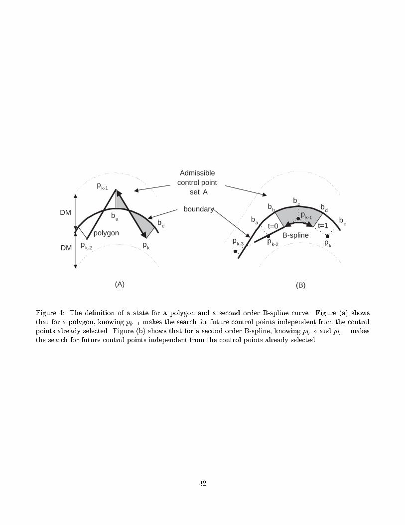
b a b e

p k-2 p k

(A)

p k-1

DM

DM

Admissible control point

set A

boundary

polygon

(B)

b a b e

p k-2 p k

p k-1

b b

b c b d

t=0 t=1

p k-3

B-spline

Figure 4: The de�nition of a state for a polygon and a second order B-spline curve. Figure (a) showsthat for a polygon, knowing pk�1 makes the search for future control points independent from the controlpoints already selected. Figure (b) shows that for a second order B-spline, knowing pk�2 and pk�1 makesthe search for future control points independent from the control points already selected.

32

t'=0

t'=1

t'=8

t'=2

t'=7

p = p

p

0 1

2

p3

Qk

Q (p ,p ,p ,t)323 4

Q5

Q6

Q7

Q8

Q1

Q2

Control point (k=0,1,...9)pk

p4

p5

p6

p7

p8

p 9

3 44 5Q (p ,p ,p ,t)

Curve segment

Knot (t'=k)

Double control point

t=t'-k+1=0...1(k=1,...8)

Figure 5: A second degree B-spline curve with 8 curve segments Qk and a double control point at thebeginning of the curve.33

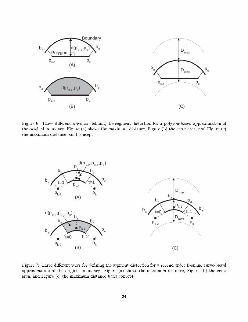
(A)

b a b e

p k-1 p k

b a

b e

p k-1 p k

b a b e

p k-1

p k

D max

(B) (C)

Boundary

Polygon

D max

d(p k-1 ,p k )

d(p k-1 ,p k )

Figure 6: Three di�erent ways for de�ning the segment distortion for a polygon-based approximation ofthe original boundary. Figure (a) shows the maximum distance, Figure (b) the error area, and Figure (c)the maximum distance band concept.

(A)

b a b e

p k-2 p k

p k-1

b b

b c b d

t=0 t=1

(B)

b a b e

p k-2 p k

p k-1

b b

b c b d

t=0 t=1

d(p k-2

,p k-1

,p k )

d(p k-2

,p k-1

,p k )

(C)

b a b e

p k-2 p k

p k-1

b b

b c b d

t=0 t=1

D max

D max

Figure 7: Three di�erent ways for de�ning the segment distortion for a second order B-spline curve-basedapproximation of the original boundary. Figure (a) shows the maximum distance, Figure (b) the errorarea, and Figure (c) the maximum distance band concept.34

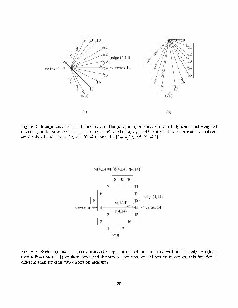
1

2

3

4

5

6

7

8 9 10

11

12

13

14

15

16

171

2

3

4

5

6

7

8 9 10

11

12

13

14

15

16

17

(a) (b)

0/18 0/18

vertex 4

edge (4,14)

vertex 14

Figure 8: Interpretation of the boundary and the polygon approximation as a fully connected weighteddirected graph. Note that the set of all edges E equals f(ai; aj) 2 A2 : i 6= jg. Two representative subsetsare displayed: (a) f(a4; aj) 2 A2 : 8j 6= 4g and (b) f(a8; aj) 2 A2 : 8j 6= 8g.

1

2

3

4

5

6

7

8 9 10

11

12

13

14

15

16

17

0/18

vertex 4 vertex 14r(4,14)

d(4,14)

w(4,14)=F{d(4,14), r(4,14)}

edge (4,14)

Figure 9: Each edge has a segment rate and a segment distortion associated with it. The edge weight isthen a function (Ff�g) of these rates and distortion. For class one distortion measures, this function isdi�erent than for class two distortion measures. 35

Switched

Order

1

2

3

4

5

6

7

8 9 10

11

12

13

14

15

16

171

2

3

4

5

6

7

8 9 10

11

12

13

14

15

16

17

Switched

Order

0/18 0/18Figure 10: Examples of polygons with rapid changes in direction.

1

2

3

4

5

6

7

8 9 10

11

12

13

14

15

16

171

2

3

4

5

6

7

8 9 10

11

12

13

14

15

16

17

(a) (b)

0/18 0/18

Figure 11: Interpretation of the boundary and the polygon approximation as a weighted directed acyclicgraph. Note that the set of all edges E equals f(ai; aj) 2 A2 : i < jg. Two representative subsets aredisplayed: (a) f(a4; aj) 2 A2 : 8j > 4g and (b) f(a8; aj) 2 A2 : 8j > 8g.36

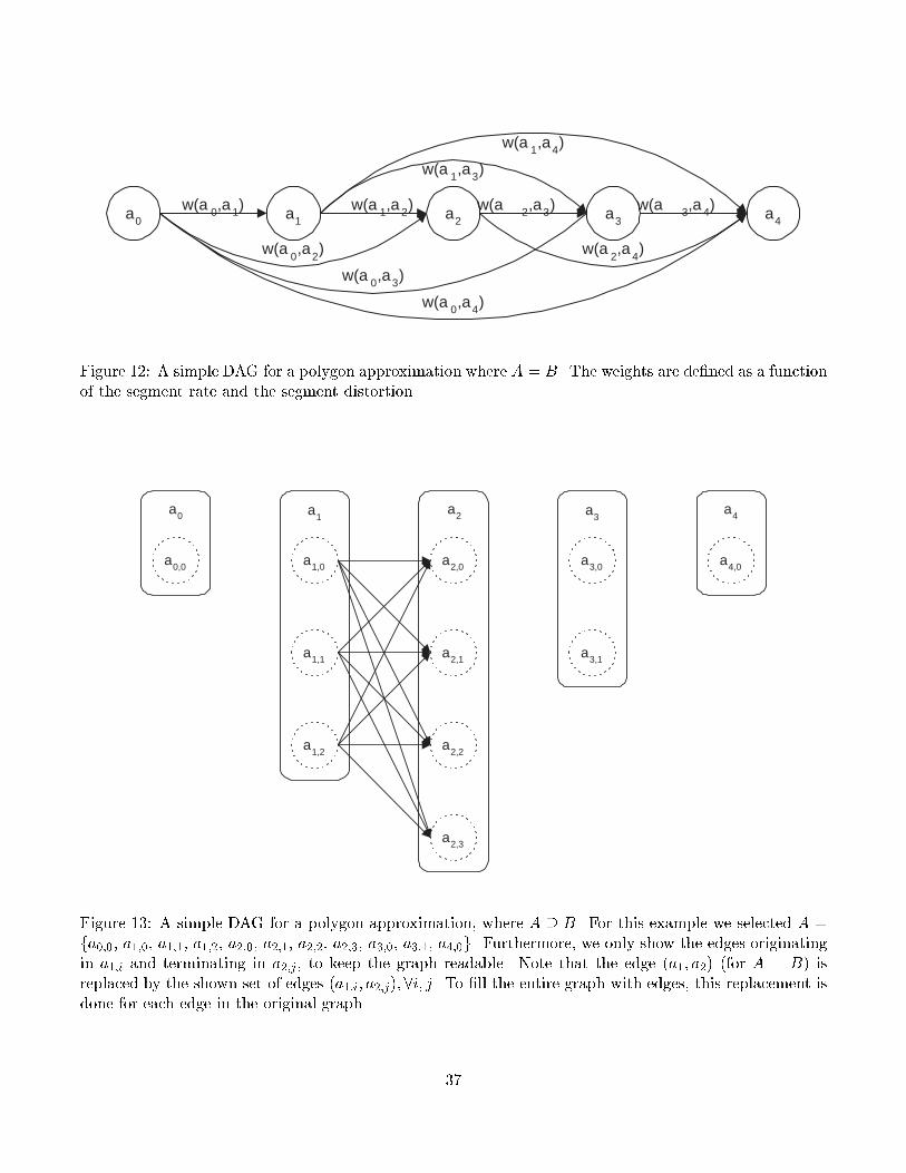
a 0 a 1 a 2 a 3 a 4

w(a 0 ,a 4 )

w(a 0 ,a 1 )

w(a 0 ,a 3 )

w(a 0 ,a

2 )

w(a 1 ,a 2 ) w(a 2 ,a 3 ) w(a 3 ,a 4 )

w(a 1 ,a 4 )

w(a 2 ,a

4 )

w(a 1 ,a 3 )

Figure 12: A simple DAG for a polygon approximation where A = B. The weights are de�ned as a functionof the segment rate and the segment distortion.a 0,0 a 1,0 a 2,0 a 3,0 a 4,0

a 1,1

a 1,2

a 2,1

a 2,2

a 2,3

a 3,1

a 1

a 2 a 3

a 4 a 0

Figure 13: A simple DAG for a polygon approximation, where A � B. For this example we selected A =fa0;0, a1;0; a1;1; a1;2; a2;0; a2;1; a2;2; a2;3; a3;0; a3;1; a4;0g. Furthermore, we only show the edges originatingin a1;i and terminating in a2;j, to keep the graph readable. Note that the edge (a1; a2) (for A = B) isreplaced by the shown set of edges (a1;i; a2;j);8i; j. To �ll the entire graph with edges, this replacement isdone for each edge in the original graph. 37

a 0 ,a

0

a 0 ,a 1

a 1 ,a 2

a 2 ,a 3

a 3 ,a 4

w(a 0 ,a 0 ,a 1 )

a 4 ,a 4

a 0 ,a 2

a 0 ,a 3

a 0 ,a 4

a 1 ,a 3

a 1 ,a 4 a 2 ,a 4

w(a 0 ,a 1 ,a 2 )

w(a 1 ,a 2 ,a 3 )

w(a 2 ,a 3 ,a 4 )

w(a 3 ,a 4 ,a 4 )

Figure 14: A simple DAG for a second order B-spline approximation, where A = B. We only label the �vetop edges with their respective weight function, but clearly, each edge has a weight function associated.

38

Dmax

Dmax

R*( )

Dmax

R*( )

maxR

*

Figure 15: The R�(Dmax) function, which is a non-increasing function exhibiting a staircase characteristic.The selected Rmax falls onto a discontinuity and therefore the optimal solution is of the form R�(D�max) <Rmax, instead of R�(D�max) = Rmax.β

α p k-2

p k-1

p k

Figure 16: A simple second order DPCM scheme is used to encode the control points. The angle � musttake a value out of the following set: f�90;�45; 45; 90g. This is encoded with two bits. The length � is anumber between 1 and 15 and is encoded using between 2 and 5 bits.39

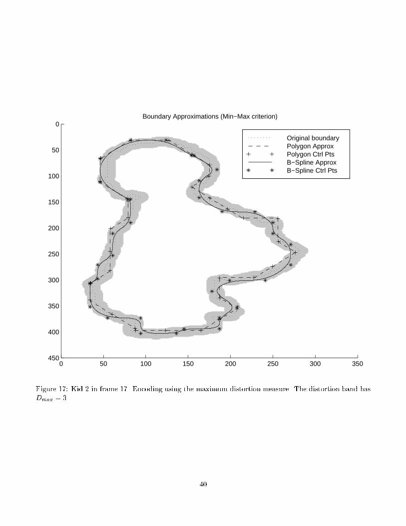
0 50 100 150 200 250 300 350

0

50

100

150

200

250

300

350

400

450

Boundary Approximations (Min−Max criterion)

Original boundaryPolygon Approx Polygon Ctrl Pts B−Spline Approx B−Spline Ctrl Pts

Figure 17: Kid 2 in frame 17. Encoding using the maximum distortion measure. The distortion band hasDmax = 3.40

0.5 1 1.5 2 2.5 3600

800

1000

1200

1400

1600

1800

2000R−D curves for 100 frames of the "Kids" sequence

Dmax

bits

Min Max, A=B, PolygonMin Max, Polygon Min Max, Spline

Figure 18: Average operational rate distortion curves for the �rst 100 frames of the "Kids" sequence.41

Figure 19: The original � plane for the 17-th frame in the sequence.

42

Figure 20: The encoded � plane for the 17-th frame in the sequence using Dmax = 0:8. The algorithmrequired 858 bits resulting in a dn of 0.0257.

43

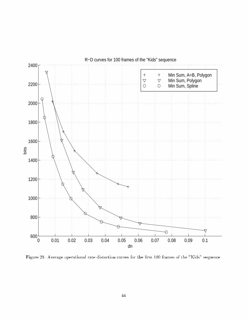
0 0.01 0.02 0.03 0.04 0.05 0.06 0.07 0.08 0.09 0.1600

800

1000

1200

1400

1600

1800

2000

2200

2400R−D curves for 100 frames of the "Kids" sequence

dn

bits

Min Sum, A=B, PolygonMin Sum, Polygon Min Sum, Spline

Figure 21: Average operational rate distortion curves for the �rst 100 frames of the "Kids" sequence.44

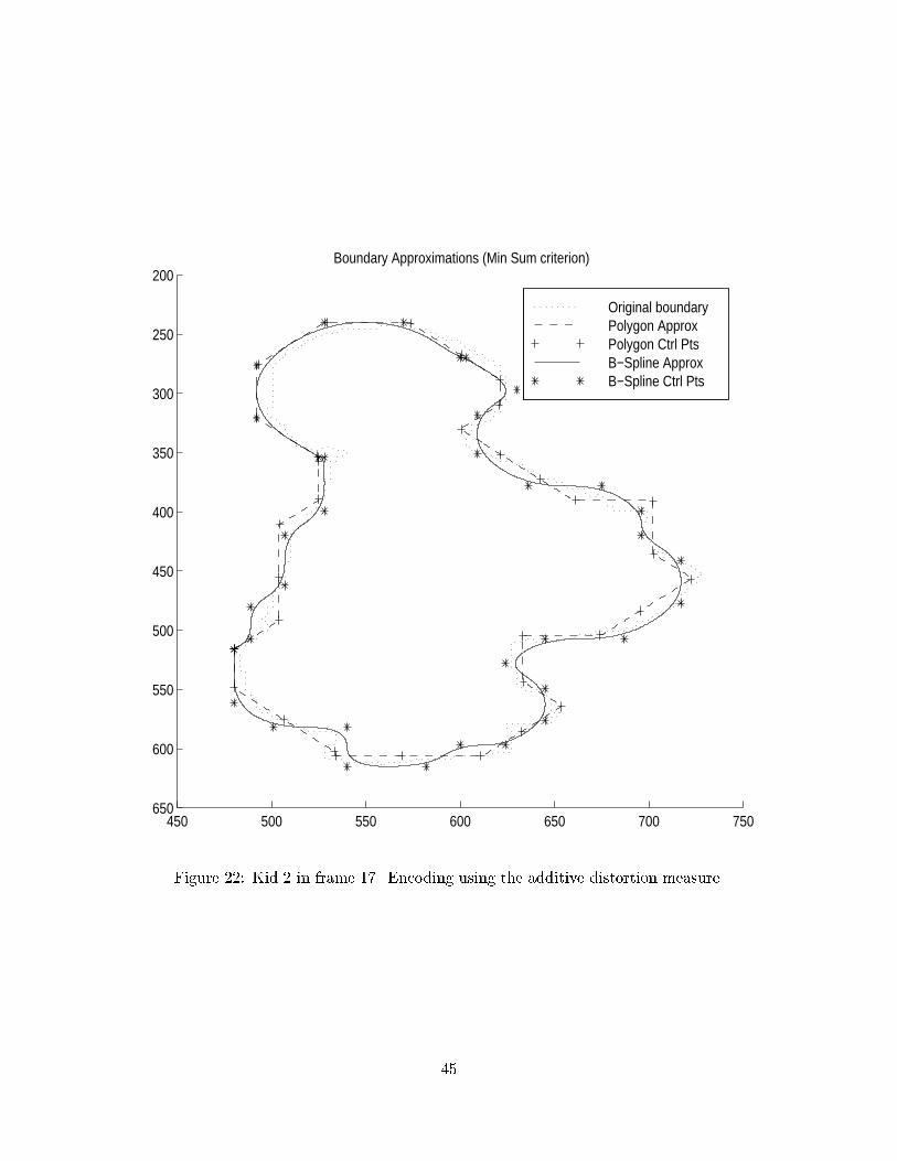
450 500 550 600 650 700 750

200

250

300

350

400

450

500

550

600

650

Boundary Approximations (Min Sum criterion)

Original boundaryPolygon Approx Polygon Ctrl Pts B−Spline Approx B−Spline Ctrl Pts

Figure 22: Kid 2 in frame 17. Encoding using the additive distortion measure.45

0 0.01 0.02 0.03 0.04 0.05 0.06 0.07 0.08 0.09 0.1400

600

800

1000

1200

1400

1600

1800

2000

2200

2400R−D curves for 100 frames of the "Kids" sequence

dn

bits

Min Max, A=B, Polygon Min Sum, A=B, Polygon Min Max, Polygon Min Max, Spline Min Sum, Polygon Min Sum, Spline Min Sum, Spline, improved code table

Figure 23: Average operational rate distortion curves for the �rst 100 frames of the "Kids" sequence.46

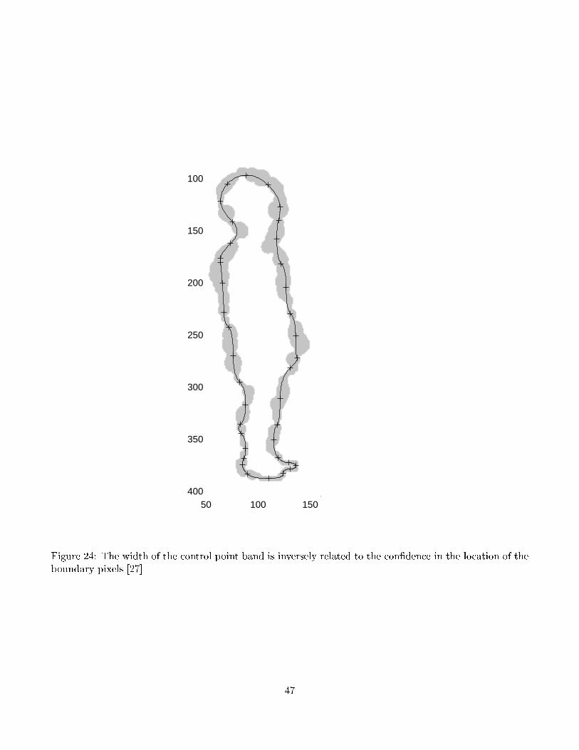
50 100 150

100

150

200

250

300

350

400

Figure 24: The width of the control point band is inversely related to the con�dence in the location of theboundary pixels [27].47