Operational Data to Assess Mobility and Crash Experience ...

Operational Data to Assess Mobility and Crash Experience during Winter ConditionsFinal ReportOctober 2018

WIMS

Sponsored byIowa Department of Transportation (InTrans Project 14-523)Midwest Transportation CenterU.S. DOT Office of the Assistant Secretary for Research and Technology

About CWIMSThe Center for Weather Impacts on Mobility and Safety (CWIMS) focuses on research to find better and safer ways to travel whenever weather is a problem. CWIMS is an Iowa State University Center administered by the Institute for Transportation.

About MTCThe Midwest Transportation Center (MTC) is a regional University Transportation Center (UTC) sponsored by the U.S. Department of Transportation Office of the Assistant Secretary for Research and Technology (USDOT/OST-R). The mission of the UTC program is to advance U.S. technology and expertise in the many disciplines comprising transportation through the mechanisms of education, research, and technology transfer at university-based centers of excellence. Iowa State University, through its Institute for Transportation (InTrans), is the MTC lead institution.

About InTransThe mission of the Institute for Transportation (InTrans) at Iowa State University is to develop and implement innovative methods, materials, and technologies for improving transportation efficiency, safety, reliability, and sustainability while improving the learning environment of students, faculty, and staff in transportation-related fields.

ISU Non-Discrimination Statement Iowa State University does not discriminate on the basis of race, color, age, ethnicity, religion, national origin, pregnancy, sexual orientation, gender identity, genetic information, sex, marital status, disability, or status as a U.S. veteran. Inquiries regarding non-discrimination policies may be directed to Office of Equal Opportunity, 3410 Beardshear Hall, 515 Morrill Road, Ames, Iowa 50011, Tel. 515-294-7612, Hotline: 515-294-1222, email [email protected].

NoticeThe contents of this report reflect the views of the authors, who are responsible for the facts and the accuracy of the information presented herein. The opinions, findings and conclusions expressed in this publication are those of the authors and not necessarily those of the sponsors.

This document is disseminated under the sponsorship of the U.S. DOT UTC program in the interest of information exchange. The U.S. Government assumes no liability for the use of the information contained in this document. This report does not constitute a standard, specification, or regulation.

The U.S. Government does not endorse products or manufacturers. If trademarks or manufacturers’ names appear in this report, it is only because they are considered essential to the objective of the document.

Iowa DOT Statements Federal and state laws prohibit employment and/or public accommodation discrimination on the basis of age, color, creed, disability, gender identity, national origin, pregnancy, race, religion, sex, sexual orientation or veteran’s status. If you believe you have been discriminated against, please contact the Iowa Civil Rights Commission at 800-457-4416 or the Iowa Department of Transportation affirmative action officer. If you need accommodations because of a disability to access the Iowa Department of Transportation’s services, contact the agency’s affirmative action officer at 800-262-0003.

Technical Report Documentation Page

1. Report No. 2. Government Accession No. 3. Recipient’s Catalog No.

InTrans Project 14-523

4. Title and Subtitle 5. Report Date

Operational Data to Assess Mobility and Crash Experience during Winter

Conditions

October 2018

6. Performing Organization Code

7. Authors 8. Performing Organization Report No.

Zachary Hans (orcid.org/0000-0003-0649-9124), Neal Hawkins

(orcid.org/0000-0003-0618-6275), Peter Savolainen (orcid.org/0000-0001-

5767-9104), and Emira Rista (orcid.org/0000-0003-2986-5940)

InTrans Project 14-523

9. Performing Organization Name and Address 10. Work Unit No. (TRAIS)

Center for Weather Impacts on Mobility and Safety

Institute for Transportation

Iowa State University

2711 South Loop Drive, Suite 4700

Ames, IA 50010-8664

11. Contract or Grant No.

Part of DTRT13-G-UTC37

12. Sponsoring Organization Name and Address 13. Type of Report and Period Covered

Iowa Department of Transportation

800 Lincoln Way

Ames, IA 50010

Midwest Transportation Center

2711 S. Loop Drive, Suite 4700

Ames, IA 50010-8664

U.S. Department of Transportation

Office of the Assistant Secretary

for Research and Technology

1200 New Jersey Avenue, SE

Washington, DC 20590

Final Report

14. Sponsoring Agency Code

90-00-TRAF-015

15. Supplementary Notes

Visit www.intrans.iastate.edu for color pdfs of this and other research reports.

16. Abstract

The primary objective of this research project was to broadly investigate potential applications of expanded maintenance data

(from automated vehicle location [AVL] and roadway image capture technology installed on snowplows) and traffic data (from

crowdsourced INRIX probe vehicles) in Iowa throughout multiple winter weather events, with an emphasis on conditions before,

during, and after crash events. Other datasets were explored and integrated for demonstration purposes, including data from

existing fixed-location cameras and traffic sensors, roadway weather information systems (RWIS) data, roadway characteristics

data, and weather and maintenance crew-based operations reports.

A benefit of analyzing crash experience over multiple events is that possible trends may be identified. Overall, this project

promotes the use of extensive, rich datasets to investigate weather-related impacts on mobility and safety and evaluate possible

opportunities for improving winter maintenance operations. The Iowa DOT may use these data resources to supplement existing

efforts to monitor traffic, weather, and surface conditions and direct their corresponding actions and reactions.

17. Key Words 18. Distribution Statement

AVL—cameras—crash experience—snowplows—speed—traffic safety—

winter road maintenance

No restrictions.

19. Security Classification (of this

report)

20. Security Classification (of this

page)

21. No. of Pages 22. Price

Unclassified. Unclassified. 100 NA

Form DOT F 1700.7 (8-72) Reproduction of completed page authorized

OPERATIONAL DATA TO ASSESS MOBILITY

AND CRASH EXPERIENCE DURING WINTER

CONDITIONS

Final Report

October 2018

Principal Investigator

Zachary Hans, Senior Research Engineer and Director

Center for Weather Impacts on Mobility and Safety

Institute for Transportation, Iowa State University

Co-Principal Investigators

Neal Hawkins, Associate Director

Peter Savolainen, Safety Engineer

Institute for Transportation, Iowa State University

Research Assistant

Emira Rista

Authors

Zachary Hans, Neal Hawkins, Peter Savolainen, and Emira Rista

Sponsored by

Iowa Department of Transportation,

Midwest Transportation Center, and

USDOT/OST-R

Preparation of this report was financed in part

through funds provided by the Iowa Department of Transportation

through its Research Management Agreement with the

Institute for Transportation

(InTrans Project 14-523)

A report from

Institute for Transportation

Iowa State University

2711 South Loop Drive, Suite 4700

Ames, IA 50010-8664

Phone: 515-294-8103 / Fax: 515-294-0467

www.intrans.iastate.edu

v

TABLE OF CONTENTS

ACKNOWLEDGMENTS ............................................................................................................. ix

EXECUTIVE SUMMARY ........................................................................................................... xi

INTRODUCTION ...........................................................................................................................1

LITERATURE REVIEW ................................................................................................................4

DATA COLLECTION, PROCESSING, AND INTEGRATION ...................................................8

Roadway Data ......................................................................................................................9 Crash Data ..........................................................................................................................10

Snowplow Images ..............................................................................................................15

Snowplow AVL .................................................................................................................16 Traffic Speed Data .............................................................................................................24

Winter Maintenance Reports .............................................................................................25

NWS COOP Stations .........................................................................................................27 Roadway Weather Information Systems ...........................................................................28

ANALYSIS ....................................................................................................................................30

Interstate 80 Winter Crash Experience ..............................................................................30 Maintenance Operations ....................................................................................................33

Traffic Speed ......................................................................................................................73

CONCLUSIONS AND RECOMMENDATIONS ........................................................................81

REFERENCES ..............................................................................................................................85

vi

LIST OF FIGURES

Figure 1. Interstate 80 corridor ........................................................................................................9 Figure 2. Cost centers of interest and primary route responsibilities ............................................13

Figure 3. Cost centers of interest and Interstate responsibilities only ...........................................14 Figure 4. Snowplow images by month ..........................................................................................15 Figure 5. Snowplow images ...........................................................................................................16 Figure 6. Number of winter events ................................................................................................18 Figure 7. Example snowplow AVL data near ramp ......................................................................19

Figure 8. Example snowplow AVL data at mid-TMC, median crossover ....................................20 Figure 9. Estimated snowplow passes for eastbound Interstate 80 ................................................22 Figure 10. Estimated snowplow passes for westbound Interstate 80.............................................22 Figure 11. Comparison of total and through lane snowplow passes for westbound Interstate

80 ...................................................................................................................................23 Figure 12. NWS COOP stations along Interstate 80......................................................................28

Figure 13. Phase 1 operations (2013) ............................................................................................33 Figure 14. Phase 1 operations (2014) ............................................................................................34 Figure 15. Winter weather-related crash days (2013, 2014) ..........................................................35

Figure 16. Winter weather-related temporal distribution ..............................................................35 Figure 17. Beginning hour of Phase 1 operations, 2013 and 2014 ................................................36

Figure 18. Beginning hour of precipitation (snow), 2013 and 2014 ..............................................37 Figure 19. Phase 1, crash time comparison, 2013 and 2014 ..........................................................38 Figure 20. Last before snowplow pass, crash time interval ...........................................................40

Figure 21. First after snowplow pass, crash time interval .............................................................41 Figure 22. Snowplow pass, crash time interval (2013) ..................................................................42

Figure 23. Snowplow pass, crash time interval (2014) ..................................................................42 Figure 24. Before, after snowplow pass interval ...........................................................................44

Figure 25. Snowplow velocity and passes, speed limit less than 70 mph .....................................46 Figure 26. Snowplow velocity and passes, 70 mph speed limit ....................................................47

Figure 27. Winter weather crashes versus directional traffic volume ...........................................51 Figure 28. Winter weather crashes per million vehicle miles travelled versus snowfall ...............52 Figure 29. Winter weather crashes per million vehicle miles travelled versus plow passes .........53

Figure 30. Plow passes versus snowfall .........................................................................................53 Figure 31. Winter weather crashes per million VMT versus snow per plow pass ........................54

Figure 32. Relationship between crash frequency and snowplow passes ......................................57 Figure 33. Relationship of crash frequency and snow/snowplow pass ratio (in./pass) .................58 Figure 34. Iowa DOT camera locations .........................................................................................59 Figure 35. Example RWIS image – poor visibility........................................................................60

Figure 36. Example RWIS image – traffic congestion ..................................................................61 Figure 37. Snowplow images and crashes within one mile ...........................................................63 Figure 38. Snowplow images and crashes within one mile and one hour .....................................64

Figure 39. Snowplow image, Example 1 .......................................................................................65 Figure 40. Snowplow image versus crash location, Example 2 ....................................................66 Figure 41. Snowplow image, Example 2 .......................................................................................66 Figure 42. Snowplow image versus crash location, Example 3 ....................................................67 Figure 43. Snowplow image, Example 3 .......................................................................................68

vii

Figure 44. Snowplow image versus crash location, Example 4 ....................................................69 Figure 45. Snowplow image, Example 4 .......................................................................................69 Figure 46. Example crash average traffic speeds...........................................................................70

Figure 47. Snowplow image versus crash location, Example 5 ....................................................71 Figure 48. Snowplow image, Example 5 (eastbound) ...................................................................72 Figure 49. Snowplow image, Example 5 (westbound) ..................................................................72 Figure 50. Traffic speed overview .................................................................................................75 Figure 51. Relative traffic speed overview ....................................................................................78

LIST OF TABLES

Table 1. Interstate 80 winter crashes..............................................................................................11 Table 2. Snowplow AVL records by month ..................................................................................18 Table 3. Snowplow AVL records near reference posts .................................................................20

Table 4. Snowplow passes near reference posts ............................................................................21 Table 5. Snowplow AVL records and estimated passes near winter weather-related crashes ......24 Table 6. INRIX traffic speed records .............................................................................................25

Table 7. NWS COOP stations along Interstate 80 .........................................................................27 Table 8. Snowplow pass, crash time interval (2013) .....................................................................43

Table 9. Snowplow pass, crash time interval (2014) .....................................................................43 Table 10. Snowplow pass frequency (2013) ..................................................................................45 Table 11. Snowplow pass frequency (2014) ..................................................................................45

Table 12. Descriptive statistics ......................................................................................................49

Table 13. Groups within data .........................................................................................................50 Table 14. Simple model results, 2014 only....................................................................................55 Table 15. Fully specified model results, 2014 only .......................................................................55

ix

ACKNOWLEDGMENTS

The authors would like to thank the Midwest Transportation Center, the U.S. Department of

Transportation (DOT) Office of the Assistant Secretary for Research and Technology, and the

Iowa DOT for sponsoring this research.

The authors also want to thank the project monitor, Tina Greenfield, and the technical advisory

committee members for their guidance and insight.

xi

EXECUTIVE SUMMARY

Objective

The primary emphasis of this project was to demonstrate the integration of historic crash data

with expanded maintenance and traffic data in Iowa to better understand the winter conditions

before, during, and after crash events.

Problem Statement and Solution

Historically, the relationships among winter weather maintenance practices, safety, and mobility

have been difficult to systematically assess and quantify, particularly because monitoring and

analysis have been somewhat limited to locations with permanent infrastructure, like fixed

cameras and traffic sensors.

Data resulting from snowplow-based automated vehicle location (AVL) and traffic analytics

acquisition initiatives now make more comprehensive analysis and assessment feasible.

Background

Winter weather poses a significant transportation problem in Iowa. The Iowa Department of

Transportation (DOT) Systems Operations Bureau employs multiple strategies to ensure mobility

and safety to the traveling public on Iowa’s primary roadways, including during and after winter

weather events.

Beginning in 2010, several Iowa DOT initiatives created new opportunities to analyze traffic and

operations data, with one initiative focusing on winter maintenance operations. This initiative

involved equipping snowplows with additional equipment, such as AVL and cameras.

Another broader initiative involved acquiring traffic analytics data for more than 8,500 centerline

miles of Iowa roadways. In 2014, the Iowa DOT entered into a contract with INRIX to obtain

real-time traffic speed data through “probes,” such as mobile phones and fleet vehicles with

global positioning sensor devices.

Project Description

Multiple datasets were collected and utilized as part of this study. The following primary datasets

were used:

Iowa DOT crash data

Iowa DOT snowplow AVL data

Iowa DOT snowplow images

INRIX traffic analytics data

xii

Other datasets included the following:

Iowa DOT roadway data

Iowa DOT maintenance crew-based operations and weather reports

Iowa DOT fixed-location camera images

Iowa DOT road weather information system (RWIS) data, including Wavetronix traffic data

and fixed-location camera images

National Weather Service (NWS) Cooperative Observer Program (COOP) snowfall data

Because of the expansive nature of the datasets, the research team opted to focus on analyzing

the Interstate 80 crash experience, maintenance crew reports and snowplow AVL crash-based

data, and traffic speed data. The data utilized were collected during 2013 and 2014. Analysis was

limited to 2 hours before and after each crash.

Key Findings

Along the I-80 corridor, winter weather-related crashes were proportionally higher during the

morning hours, which may be influenced by several factors. Crashes that occur when people

are typically departing for work and school highlight the need for appropriate and accurate

motorist-directed messaging.

More crashes occurred as the time interval increased between the last snowplow pass and the

time of the crash. The snowplow pass interval of 90 minutes to 2 hours before the crash and

within 30 minutes after the crash had the single highest percentage of crashes.

The majority of winter weather-related crashes involved multiple snowplow passes within 2

hours before and after the crash. This may indicate that crashes occur early in the weather

event, during periods of high snowplow activity, and/or along multilane sections.

From a safety perspective, Phase 1 winter maintenance operations appear broadly successful

and to have occurred during appropriate times.

As snowplow frequency increases for a specific amount of snow, the volume of traffic

crashes per million vehicle miles traveled decreases. This demonstrates, in part, the safety-

related effectiveness of winter maintenance.

Recommendations for Future Research

Spatial and temporal integration of crash and image datasets may facilitate after-action

assessment and investigation of location-based conditions before and after a crash. These

conditions may also be compared to conditions in locations where no crash has occurred to

provide perspective. Better understanding of crash conditions may help assess whether

operational expectations were satisfied and if modifications should be considered.

Development of an expanded statistical model that includes additional weather-related and other

parameters may be warranted. Micro-level case studies may also be beneficial in quantifying the

impacts of extraneous factors.

xiii

Opportunities may exist to utilize localized speed monitoring coupled with weather data to

identify unstable and changing conditions, with subsequent messaging informing motorists of

traffic conditions.

Implementation Readiness and Benefits

This project promotes the use of extensive, rich datasets to investigate weather-related impacts

on mobility and safety and evaluate opportunities for improving winter maintenance operations.

In this research, new capabilities were introduced; existing capabilities were expanded; and

limitations, challenges, and potential areas for additional investigation were identified.

Ultimately, this work can help the Iowa DOT further mitigate the impacts of winter weather. The

Iowa DOT may use the resources developed in this study to supplement existing efforts to

monitor traffic, weather, and surface conditions and direct its corresponding activities.

1

INTRODUCTION

Winter weather poses a significant transportation problem in Iowa, the US, and the world. The

Federal Highway Administration (FHWA) Road Weather Management Program estimates that

more than 1,300 people are killed and 116,800 people are injured in vehicle crashes on snowy,

slushy, or icy pavements in the US annually. Furthermore, nearly 900 people are killed and

76,000 people are injured during snowfall and sleet (FHWA 2017). From 2010 through 2014 in

Iowa, more than 8,000 winter weather-related crashes occurred annually, resulting in an annual

average of more than 190 fatalities and serious injuries, 2,200 other injuries, and nearly $48

million in property damage. During this period, more than half of the severe crashes occurred on

primary (state-maintained) roadways, compared to approximately 40 percent of the other less

severe crashes.

The economic impacts of weather events are also substantial, ranging from winter operations

costs of more than $2.3 billion annually for local and state agencies (FHWA 2017) to freight

traffic delay costs estimated at more than $8 billion (Krechmer et al. 2012). In recent years, the

Iowa Department of Transportation (DOT) alone has spent more than $30 million annually on

winter operations, including labor, equipment, and materials (Iowa DOT 2017a). While the Iowa

DOT is only responsible for a fraction of the public roadways in the state (approximately 8

percent of centerline miles), these roadways represent more than 60 percent of the total state

vehicle miles of travel (VMT) and more than 90 percent of the combination truck VMT (Iowa

DOT 2017b).

The Iowa DOT Systems Operations Bureau employs multiple strategies to ensure mobility and

safety to the traveling public on Iowa’s primary roadways, including during and after winter

weather events. The Office of Maintenance coordinates with field maintenance staff to manage

maintenance operations and provide consistent, effective, and quality services. The Office of

Traffic Operations provides proactive traffic management, and the Office of Traffic and Safety

provides timely, comprehensive crash data for all public roadways (Iowa DOT 2017c).

Beginning in 2010, several Iowa DOT initiatives created new opportunities to analyze traffic and

operations data, with one initiative focusing on winter maintenance operations. This initiative

involved equipping snowplows with additional equipment, such as automatic vehicle location

(AVL) and cameras. Another broader initiative involved acquiring traffic analytics data for more

than 8,500 centerline miles of Iowa roadways.

In 2010, a request for proposals (RFP) issued by the Iowa DOT was intended to help better

understand and visualize fleet movement and material usage, allow managers to direct the fleet,

facilitate use of plow data for custom reporting and improved efficiency, and provide the public

with a better winter driving experience. Trial deployment was initiated in 2011–2012. Full

deployment, which occurred in 2012–2013, included installation of AVL equipment and iPhones

(for image capture) on Iowa DOT owned plows, approximately 900 and 430 snowplows,

respectively. Specific data collected will be discussed later in this report. In 2014, in an effort to

expand traffic data collection beyond existing fixed-location sensors, the Iowa DOT entered into

a contract with INRIX to obtain real-time traffic speed data through “probes,” e.g., mobile

2

phones and fleet vehicles with global positioning sensor (GPS) devices. As part of this contract,

historic traffic data were also obtained (INRIX 2014).

Through these initiatives as well as previous efforts to expand the infrastructure of monitoring

equipment, the Iowa DOT has explored a more public facing strategy to improve mobility and

safety. Specifically, this strategy is to provide the best and most comprehensive information

available to motorists, ideally assisting them in making better decisions regarding travel,

especially during winter weather. For example, the Track a Plow website provides the location

and number of plows, the view from each plow, road conditions, traffic, closures, and radar on

an interactive map (Iowa DOT 2017d). Additional information, such as incidents, cameras,

traffic speeds, and road conditions, is available through http://511ia.org/.

Because a highway agency can only do so much to impact human behavior, more traditional

agency responsibilities, like winter maintenance, should also be considered to improve mobility

and safety. Historically, the relationships among winter weather maintenance practices, safety,

and mobility have been difficult to systematically assess and quantify. Monitoring and analysis

have also been somewhat limited to locations with more permanent infrastructure, such as fixed-

location cameras and traffic sensors. The AVL and traffic analytics acquisition initiatives make

more comprehensive analysis and assessment feasible, facilitating more refined and broader

location-specific analyses. The Iowa DOT may use these resources to supplement existing efforts

to monitor traffic, weather, and surface conditions and direct their corresponding actions and

reactions. Through integration and review of historic crash data, the Iowa DOT may gain a better

understanding of the conditions during which crashes occur, whether these conditions are

expected based on weather and maintenance efforts, as well as whether opportunities may exist

to adjust future practices.

The primary objective of this research project was to broadly investigate potential applications of

these expanded maintenance (snowplow-based AVL and roadway images) and traffic

(crowdsourced INRIX) data in Iowa throughout multiple winter weather events, with an

emphasis on conditions before, during, and after crash events. Other datasets were explored and

integrated for demonstration purposes, such as data from existing fixed-location cameras and

traffic sensors, roadway weather information systems (RWIS) data, roadway characteristics data,

and weather and maintenance crew-based operations reports. A benefit of analyzing crash

experience during multiple events is that possible trends may be identified, while a limitation is

that the unique nature of and circumstances surrounding each event may not necessarily be

addressed, as may be done in an after-action review.

The remainder of this report is divided into four chapters:

1. Literature Review provides an overview of past studies related to weather maintenance and

operations, traffic safety, and mobility.

2. Data Collection, Processing, and Integration details the methodological approaches used to

prepare the various datasets for analysis, including challenges and limitations.

3

3. Analysis focuses on three primary areas: general crash experience along the Interstate 80

corridor; the relationships between crash experience and maintenance operations-related data,

roadway characteristics, and snowfall; and traffic speed profiles with respect to crash

experience.

4. Conclusions and Recommendations discusses some key project findings and, based on these

findings, suggests areas where additional analysis may be warranted.

4

LITERATURE REVIEW

Crashes are comprised of three main components: driver behavior, roadway environment, and

vehicles. During winter weather events, i.e., events that can include the presence of wind,

precipitation in either liquid or solid forms, or ice, all three of these components are affected to

some extent, thus potentially creating more opportunities for crashes.

Through winter weather maintenance and operations, i.e., the operation of snowplows that

remove snow from the roads and distribute salt and other chemicals that melt the snow and ice

remnants, state DOTs can aid in the improvement of roadway conditions during such winter

weather events. Cleaner roads provide a better environment for drivers to travel and also offer

drivers a sense of security while driving. However, two major questions regarding winter

weather roadway maintenance and operations arise: (1) How does snowfall affect roadway

safety? and (2) In response to snow and other weather events, how does the presence and/or

frequency of snowplows on the roadway system affect safety?

Two early studies examined the relationship between crash rate and risk and winter roadway

maintenance operations. A study by Kuemmel and Hanbali (1992) examined the crash rate

before and after roadway maintenance during weather events for a random sample of 520 miles

of two-lane undivided highways and 50 miles of divided highways. The roadway samples and

data came from New York, Illinois, Minnesota, and Wisconsin. Accident rates were computed

utilizing traffic volumes and segment length at hourly intervals for 12 hours before and 12 hours

after the last salt spreading time (taken as hour 0). The before and after analyses were conducted

separately for freeway sections and two-lane sections utilizing the Poisson method, the paired t-

test, and a conservative method called Revised Decision Criteria. These analyses demonstrated

that the use of salt, or salt combined with other chemicals, reduced the crash rate (crashes/million

vehicle miles travelled) for total crashes, as well as the severity. A benefit-cost analysis further

demonstrated that roadway maintenance helped reduce costs related to crashes as well as travel

time.

A Swedish study (Norrman et al. 2000) examined the quantitative relationships between road

slipperiness, crash risks, and winter roadway maintenance (WRM) activity in a southern Swedish

region where WRM is performed to increase road safety. Road conditions at the time of an

accident were classified as one of 10 different types of slippery conditions (or as not slippery),

based on meteorological data from RWIS stations. Crash data were obtained from police reports

compiled by the Swedish National Road Administration and included crashes of all types and

severity. The number of reported traffic accidents during the winter were 67 in 1991–92, 84 in

1993–94, and 95 in 1995–96. As maintenance action can take several hours and traffic accidents

are instant events, a day was divided into four different periods: morning, day, evening, and

night. If there had been any maintenance performed during the period in which the accident

occurred, the road condition was considered as improved. The final choice of these three winters

was based on the different climatology and WRM reports available. Of the 246 accidents during

the three winters, 50% were related to slippery road conditions, either in the accident reports or

by the classification. Twenty percent of the accidents were verified as slipperiness related, both

by the accident reports and the classified RWIS data. Overall, crash risk was different for various

5

types of road slipperiness with the highest risk being associated with slipperiness caused by rain

or sleet. These conditions were also associated with high levels of WRM activities.

During the last decade, numerous studies have been conducted that have examined the impact of

weather events, such as snow and ice, and weather-related roadway maintenance operations on

traffic safety. One study (Black and Mote 2015) examined the association between injury and

fatality crashes and winter weather precipitation for 13 U.S. cities by utilizing crash and weather

data from 1996 to 2010. The locations were selected based on the frequency of winter weather

experiences for each city as well as what type of winter weather precipitation was experienced

(snow, sleet, and freezing rain). Weather data were collected mostly based on specific location

observations, such as at airports, whereas crash data were obtained from the National Highway

Traffic Safety Administration (NHTSA). A matched pair analysis revealed that property damage

only (PDO) collision risk increased by 19%, while injury collision risk increased by 13% during

winter precipitation when compared to control periods. Conversely, the risk of fatalities was

similar during winter weather conditions as compared to control periods. Three of the strongest

predictors for crash and injury risk were precipitation intensity, time of day, and order of the

precipitation. Crash and injury risks were higher during more intense precipitation, afternoon and

evening times of day, and during the first three precipitation events of a winter period.

Other studies (Usman et al. 2011, Shaheed et al. 2016, El-Basyouny et al. 2014) have proposed

methodologies for estimating the effects of various traffic, roadway, and weather-related

variables on crash frequency, type, and severity. Usman et al. 2011 investigated the safety effects

of winter road maintenance, weather, and road characteristics utilizing data from October 2000

to April 2006 from 31 maintenance routes in the province of Ontario, Canada. Several models

were examined including Poisson lognormal, negative binomial, and generalized negative

binomial, and calibrated. Results showed that the best performing model, in terms of the Akaike

information criterion (AIC), was the generalized negative binomial regression. Roadway surface

index, visibility, precipitation, and exposure variables were significant, with poorer roadway

surface conditions and visibility, higher precipitation, and exposure being associated with a

higher number of crashes. Earlier winter months were found to be associated with higher crash

frequency. These models were later utilized in case studies (Usman et al. 2012) to illustrate the

potential applications for quantifying the safety benefits of winter roadway maintenance. Among

the benefits examined were the shortening of bare pavement recovery time, changing of

maintenance operation deployment time, and increasing level of service (LOS) standards.

Shaheed et al. (2016) examined the factors affecting occupant injury severity in winter seasons,

taking into account the within-crash and between-crash correlation of injury severity. This

required the development of full Bayesian hierarchical multinomial logit models for winter-

weather crashes, non-weather-related crashes, and total crashes. Data were collected for four

winter periods in Iowa, nesting the person-level information within the crash-level information.

The results showed that the demographic and person-level (driver/passenger) information with

regard to seat belt and airbag use was significant. Also significant were road junction type, first

harmful event, and major crash cause. Winter weather-related variables, such as visibility,

pavement, and air temperature, were also found to be significant and have an impact on crashes,

as previously established for crash frequency and type (Usman et al. 2011, El-Basyouny et al.

2014).

6

El-Basyouny et al. (2014) investigated the impact that weather elements, specifically unexpected

precipitation events such as rain or snow, have on crash type. Five years of daily weather and

crash data from the city of Edmonton, Alberta, Canada, were used to estimate multivariate

models in a full Bayesian context via Markov Chain Monte Carlo simulation. The Poisson

lognormal model proved to be the best fit, based on the deviance information criterion (DIC),

which agreed with previous study results (Usman et al. 2011). The variables found to be

significant were snow, temperature, and sudden precipitation events, which were seen to be

associated with three crash types, namely following-too-close, stop sign violation, and run-off-

road crashes. Wind and rain were found to be mostly insignificant, except for a few crash types.

The day of the week was found to be statistically significant, indicating a possible weekly

variation in exposure. The information presented in the study could be useful to transportation

authorities in informing the public with regard to the risk associated with various crash types

during particular winter weather conditions. Information on road maintenance during winter

weather conditions could be useful to drivers in planning their routes. A study by Menard et al.

(2012) presented an approach for tracking snowplows during winter weather events via hardware

designed to be installed in the plows, which relays the plow position to the real-time traffic

simulator FreeSim, without human interaction. The data are then analyzed and displayed in the

form of color-coded lines with the time elapsed since a roadway was plowed.

Other studies have reported the practices of winter weather maintenance and their operational

benefits. A 2012 report (Murphy et al. 2012) summarized the efforts that have been undertaken

in Idaho with the development of the Winter Maintenance Performance Measures System, which

included 87 RWIS sites. The Idaho Transportation Department (ITD) evaluated the performance

levels of its winter maintenance operations and adjusted the practices accordingly to increase

operational efficiencies. ITD also developed a system to collect and track maintenance data on

salt usage, liquid quantity usage, application rates, and plow down/up time. This information was

previously collected manually and, therefore, was time consuming to gather and prone to error.

A benefit-cost study by Koeberlein et al. (2014) reported the benefits resulting from the efforts

undertaken by ITD to optimize maintenance practices through a data-driven process. The paper

compared winter driving crash statistics between 2010 and 2013 on roadway segments prior to

and after the deployment of RWIS sites and then computed a benefit/cost metric. The benefit-

cost ratio for this study period was found to be 22, which illustrates the benefits of strategically

deployed RWIS sites and proper utilization of data. Additionally, winter weather-related

fatalities on the segments analyzed were shown to be significantly reduced during the study

period. A Minnesota case study was utilized to demonstrate the methodologies developed by Ye

et al. (2013) in order to estimate the benefits of winter weather maintenance, namely safety

improvements, savings in travel time, and fuel savings. The cost-benefit ratio of winter highway

operations was found to be 6.2, and the benefits were estimated to be $227 million, with $168

million in safety benefits, $48 million in fuel savings, and $11 million in mobility improvement.

A paper by McNamara et al. (2017), developed three performance measures and incorporated

them into a series of dashboards to be used for data-driven decision making for winter weather

management and operations. The paper summarizes the efforts made to collect and integrate

weather data, namely the precipitation amounts, net short wave solar radiation, average surface

skin temperature, and crowdsourced probe vehicle data. Once the data were collected and

visualized, several parameters were directly measurable from the data, such as weather event

7

duration, time to first impact, time to maximum impact, primary recovery time, and full recovery

time. These parameters were used to compute metrics that are more useful for assessing storm

intensity and relative network recovery, easy to compute, and intuitive to communicate for rapid

after-action reviews of storms. These metrics included the recovery time normalized to storm

duration, the duration of overall impact on traffic, and the material usage divided by the impact

on traffic. Finally, the use of these metrics was illustrated by analyzing the eight largest winter

storm events occurring in Indiana during the 2015–2016 winter season.

An Institute for Transportation report (Barajas et al. 2017) summarizes the efforts made in two

similar projects to develop models that could predict the performance of Iowa DOT maintenance

operations during winter weather conditions. During the first project, a model was developed to

estimate speed reductions based on weather information and normal conditions maintenance

schedules. During a prior project, a sequential Bayesian dynamic model was estimated to predict

speed changes relative to baseline speeds under normal conditions, utilizing winter weather

variables such as snow type, temperature, and wind gusts that were measured by roadside

weather stations. However, this model was not able to accommodate temporal heterogeneity;

therefore it was improved to achieve real-time prediction of traffic speed changes with realistic

uncertainty measures. Two different sources of data were used: RWIS and automated weather

observing systems (AWOS). Additionally, maintenance crew reports were utilized to identify

winter weather throughout the year. The model framework allowed for the accommodation of

interactions between atmospheric variables and roadway pavement conditions as well as

temporal dynamics. The results showed that traffic speeds depend on location, day of the week,

and time of day. Second, the effects of winter weather variables and existing roadway conditions

on traffic speed changes are spatially and temporally variable. The report presented the potential

for obtaining real-time feedback and forecasts.

The second project, which largely depended on the results of the first one, used traffic data and

limited weather information for the development of models that detect abnormal traffic patterns

and predict speeds and volumes at any given location. The second project utilized both

Wavetronics and INRIX data collected in 2013 and 2014 on Interstates 35 and 80 and on US 65

and IA 5 in Des Moines. Data from each location and day of the week were analyzed using a

multivariate quantile estimator for extreme value detection. One of the products of this project

was an online interactive app that visualizes results and can aid the Iowa DOT in making

informed decisions regarding winter weather maintenance operations.

8

DATA COLLECTION, PROCESSING, AND INTEGRATION

This chapter provides an overview of the methodological approaches used to prepare the various

datasets for analysis, including challenges and limitations. Multiple datasets were collected and

utilized as part of this study. The primary datasets used throughout this study were as follows:

Iowa DOT crash data

Iowa DOT snowplow AVL data

Iowa DOT snowplow images

INRIX traffic analytics data

Other datasets used included the following:

Iowa DOT roadway data

Iowa DOT maintenance crew-based operations and weather reports

Iowa DOT fixed-location camera images

Iowa DOT RWIS data, including Wavetronix traffic data and fixed-location camera images

National Weather Service (NWS) Cooperative Observer Program (COOP) snowfall data

Because of the expansive nature of the snowplow AVL data, the Iowa DOT Office of

Maintenance recommended limiting AVL and traffic speed analysis to Interstate 80. Interstates,

in general, are good candidates for traffic speed analysis because of the high-quality INRIX data

available. Interstate 80 (including concurrencies) also represents approximately 39 percent of the

total statewide Interstate centerline miles and, in 2014, carried 47 percent of the total Interstate

VMT (48 percent with a speed limit of 70 mph and 44 percent with a speed limit less than 70

mph). Figure 1 presents the Interstate 80 corridor across the state. Concurrencies exist with

Interstate 29 in western Iowa (Pottawattamie County) and Interstate 35 in central Iowa (Polk

County). The subsequent analyses discussed may include either the entire corridor or a portion

beginning east of the Interstate 29 concurrency in Pottawattamie County (approximately

reference post four).

9

Figure 1. Interstate 80 corridor

Prior to discussing the primary datasets used in analyses, the roadway datasets, which serve as a

frame of reference for analyses as well as provide valuable supplemental attributes, will be

introduced.

Roadway Data

Roadway Characteristics

The Iowa DOT Geographic Information Management System (GIMS) roadway database

contains roadway characteristics, directionally and for a roadway as a whole, for all public roads

within Iowa. Temporal snapshots are produced annually.

The roadway segments for the primary study corridor, Interstate 80, were extracted from the

GIMS roadway database for the analysis years. Attributes included, but were not limited to,

surface width, median type and width, shoulder type and width, number of lanes and lane type,

curvature, grade, and average annual daily traffic (AADT). Not all attributes were directional in

nature and, instead, represented the entire roadway cross-section. Therefore, lane information

was separated to reflect the individual characteristics by direction, or assumptions were made to

derive equivalent directional representations. For example, a 50/50 directional split was assumed

for all traffic data, and median attributes were used for both directions of travel since the two

directions share the same median. The number of lanes and lane type were manually verified and

collected for each segment of Interstate 80.

10

GIMS-based roadway attributes will be used in conjunction with multiple other datasets, such as

crashes and reference posts.

Reference Posts

Directional reference posts, also known as mileposts, along Interstate 80 (and concurrencies),

were extracted from an Iowa DOT geographic information system (GIS)-based reference post

dataset containing all primary routes. Reference posts are located at an interval of approximately

one mile and can either be real (physically exist along the roadway) or virtual (do not physically

exist and are only used as a reference within GIS). Even though concurrent routes exist along

Interstate 80, the reference post values are sequential, with no discontinuities, from Nebraska to

Illinois, ranging from 0 to 306. In a limited number of instances, where no official reference post

existed in the database for one direction of travel, a reference post record was manually added

for analysis purposes.

The reference post dataset will be used, in part, as a common frame of reference for data

integration and aggregation in some analyses.

Crash Data

The Iowa DOT crash database was obtained from the Office of Traffic and Safety. It consists of

reported crashes on all public roads resulting in an injury or minimum estimated property

damage of at least $1,500. The crash database includes both data elements coded on the crash

report as well as several derived elements. Attributes are provided for the crash event as a whole,

at the driver/vehicle level, and at the person level (e.g. drivers, injured motor vehicle occupants,

and non-motorists).

Crash locations are geocoded by either law enforcement or the Department of Motor Vehicles

through use of the Incident Location Tool (ILT) within the Traffic and Criminal Software

(TraCS). ILT is a GPS-enabled, GIS-based tool, which utilizes several reference layers,

including the Iowa DOT GIMS roadway database. Divided roadways in the GIMS roadway

database are represented by a single centerline and not directionally. As a result, all crashes are

geocoded to a common centerline, regardless of direction of travel. The manner in which this

was addressed will be discussed later.

Traditionally, crash analysis for the Iowa DOT winter maintenance period spans portions of two

calendar years, beginning on October 15 and ending on April 15 of the following year. However,

given the availability of snowplow AVL data, snowplow images, and historic INRIX traffic data

for the study, such analysis would have been limited to the winter of 2013–2014. To expand this

analysis, crash data were extracted for the winter maintenance periods during calendar years

2013 and 2014, specifically January 1, 2013 through April 15, 2013, October 15, 2013 through

December 31, 2013, January 1, 2014 through April 15, 2014, and October 15, 2014 through

December 31, 2014. Crashes were further limited to those identified as occurring along a primary

roadway. This crash dataset was used for integration with snowplow images. A second crash

11

dataset was also prepared for crashes located along the mainline of Interstate 80 (and

concurrencies) only. Along concurrent sections, existing route and system attributes were

updated to reflect Interstate 80.

Supplemental Crash Data

Additional attributes were derived and integrated into the Interstate 80 crash dataset for use in

analysis. These attributes included a winter weather-related indicator, direction of travel, Iowa

DOT reference post, maintenance cost center, traffic message channel (TMC), roadway

characteristics, and maintenance crew and precipitation reports. Descriptions of these

supplemental attributes follow, with the exception of maintenance crew and precipitation reports,

which will be discussed independently.

Winter Weather-Related Crashes

Based on the 2001 crash report form, the Iowa DOT defines winter weather-related crashes as

those in which any of the following were reported for the crash event or for any driver/vehicle

involved in the crash:

Weather conditions: Sleet/hail/freezing rain or snow or blowing sand/soil/dirt/snow

Surface conditions: Ice or snow or slush

Vision obscured: Blowing sand/soil/dirt/snow

Because the crash dataset was limited to the winter maintenance period(s) during calendar years

2013 and 2014, only crashes satisfying this criterion, and occurring during these time periods,

were considered. A single winter weather-related crash attribute was added and populated. Table

1 presents the resulting distribution of winter weather- and non-winter weather-related crashes.

Table 1. Interstate 80 winter crashes

Type

Winter Crashes

2013 2014

Non-winter weather-related 399 543

Winter weather-related 619 590

Crash Direction

As mentioned previously, for divided roadways, all crashes are geocoded to a single centerline

representation of the roadway. Side of roadway and lane position are not reported. For analysis

purposes, and future integration with other pertinent datasets, knowledge of crash directionality

was necessary. While the Office of Traffic and Safety derives a “cardinal direction of vehicles”

attribute from reported elements on the crash report, an effort was made to confirm and update

this information, if necessary. The “initial direction of travel” attribute, which is provided on a

12

vehicular basis and indicates the direction of travel of each vehicle involved in the crash, was

key to deriving crash-level direction. Initial direction of travel values included north, south, east,

west, unknown, and not reported. A cross tabulation table was used to aggregate all vehicles

involved in the same crash. The unique crash identifier was selected as the rows (observations)

and the initial direction of travel attribute was selected as the columns. For crashes in which the

initial direction of travel was the same for all vehicles and (generally) accurately corresponded to

the orientation of the roadway, no ambiguity existed, and crash-level direction could be

immediately derived.

For a limited set of crashes, various degrees of ambiguity were present and visual inspection was

required:

Vehicles travelling in different directions, such as north and east. This could simply be a case

of the Interstate changing from north-south to east-west in orientation, and the vehicles were

actually travelling in the same direction.

Vehicle(s) direction of travel reported as unknown or not reported, alone, or in conjunction

with other valid direction(s) of travel.

Vehicles travelling in opposite directions. This could represent miscoding, cross-median

crashes, or driving in the wrong direction of travel.

Vehicles traveling in different directions, namely north and west or south and east.

Vehicle(s) traveling in a direction contrary to the orientation of the roadway.

For consistency, the crash-level direction of travel was updated as east or west for all crashes

with a systematically derived or manually populated crash-level direction. This primarily

impacted crashes along the Interstate 35 concurrency near Des Moines, where the original initial

direction of vehicle travel was predominately north and south.

Supplemental Roadway Data

Reference Posts

Reference post attributes (direction and value/mileage) were systematically assigned to each

crash in the Interstate 80 crash dataset based on crash direction and spatial proximity (nearest).

Iowa DOT Maintenance Cost Centers

Cost centers, also known as maintenance garages, represent the Iowa DOT field maintenance

offices responsible for maintaining primary roadways throughout the state. Cost centers maintain

maintenance crew-based operations and weather reports throughout the winter maintenance

period. To consider such information in crash analysis, the cost center of each crash must be

known.

13

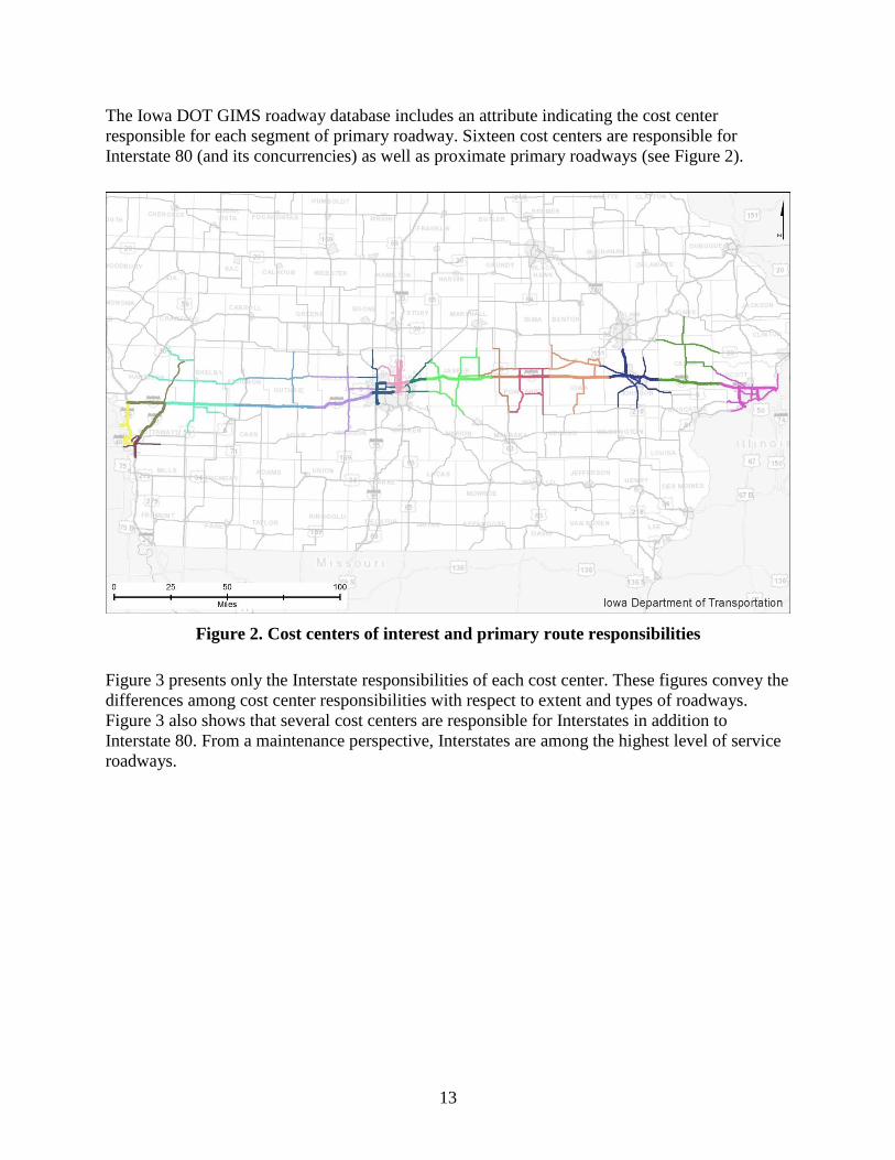
The Iowa DOT GIMS roadway database includes an attribute indicating the cost center

responsible for each segment of primary roadway. Sixteen cost centers are responsible for

Interstate 80 (and its concurrencies) as well as proximate primary roadways (see Figure 2).

Figure 2. Cost centers of interest and primary route responsibilities

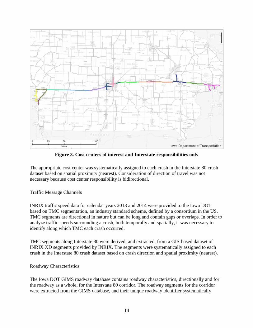
Figure 3 presents only the Interstate responsibilities of each cost center. These figures convey the

differences among cost center responsibilities with respect to extent and types of roadways.

Figure 3 also shows that several cost centers are responsible for Interstates in addition to

Interstate 80. From a maintenance perspective, Interstates are among the highest level of service

roadways.

14

Figure 3. Cost centers of interest and Interstate responsibilities only

The appropriate cost center was systematically assigned to each crash in the Interstate 80 crash

dataset based on spatial proximity (nearest). Consideration of direction of travel was not

necessary because cost center responsibility is bidirectional.

Traffic Message Channels

INRIX traffic speed data for calendar years 2013 and 2014 were provided to the Iowa DOT

based on TMC segmentation, an industry standard scheme, defined by a consortium in the US.

TMC segments are directional in nature but can be long and contain gaps or overlaps. In order to

analyze traffic speeds surrounding a crash, both temporally and spatially, it was necessary to

identify along which TMC each crash occurred.

TMC segments along Interstate 80 were derived, and extracted, from a GIS-based dataset of

INRIX XD segments provided by INRIX. The segments were systematically assigned to each

crash in the Interstate 80 crash dataset based on crash direction and spatial proximity (nearest).

Roadway Characteristics

The Iowa DOT GIMS roadway database contains roadway characteristics, directionally and for

the roadway as a whole, for the Interstate 80 corridor. The roadway segments for the corridor

were extracted from the GIMS database, and their unique roadway identifier systematically

15

assigned to each crash in the Interstate 80 crash dataset based on spatial proximity (nearest). This

ultimately provided roadway characteristics for each crash.

Snowplow Images

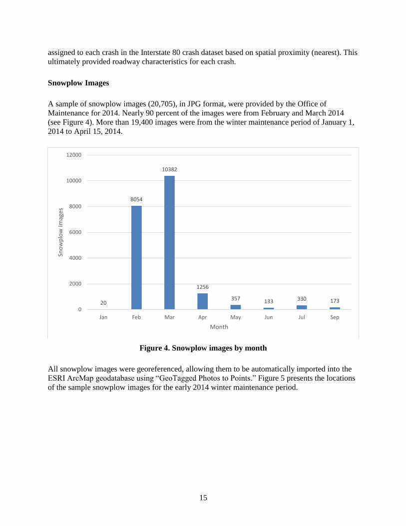
A sample of snowplow images (20,705), in JPG format, were provided by the Office of

Maintenance for 2014. Nearly 90 percent of the images were from February and March 2014

(see Figure 4). More than 19,400 images were from the winter maintenance period of January 1,

2014 to April 15, 2014.

Figure 4. Snowplow images by month

All snowplow images were georeferenced, allowing them to be automatically imported into the

ESRI ArcMap geodatabase using “GeoTagged Photos to Points.” Figure 5 presents the locations

of the sample snowplow images for the early 2014 winter maintenance period.

20

8054

10382

1256

357 133 330 173

0

2000

4000

6000

8000

10000

12000

Jan Feb Mar Apr May Jun Jul Sep

Sno

wp

low

Imag

es

Month

16

Figure 5. Snowplow images

The images also possessed a timestamp in their filename, which was imported as an attribute

within the geodatabase. With some minor manipulation and use of the “Convert Time Field”

tool, a standard date/time attribute was created, facilitating temporal querying and comparison. A

combination of spatial and temporal proximity will be used to integrate snowplow images and

the statewide crash dataset.

Snowplow images are currently archived on the Iowa Environmental Mesonet, and a portion of

the images are available through the Iowa DOT Open Data portal.

Snowplow AVL

When the research project was initiated, no formal process existed for external distribution or

sharing of snowplow AVL data. AVL records were managed in an Oracle Spatial database

within the Iowa DOT. Access to the data was limited to database exports. Because of

compatibility issues between the relational databases being used, only data in comma separated

value (CSV) format could be processed. This resulted in some unintended consequences of

extremely large export file sizes that could contain additional, variable numbers of commas

within some fields. Through multiple iterations, tools were developed to address the file size and

comma issues, ultimately allowing the data to be imported into a Microsoft SQL Server database.

Records not imported properly were manually addressed. Since this study was initiated,

significant advancements have since been made by the Iowa DOT to improve external access to

the snowplow AVL data, such as through the Iowa DOT Open Data portal.

17

While every attempt was made to ensure that all AVL data provided were represented, given the

number of records, it was impossible to completely confirm. Additionally, it was assumed that

all pertinent AVL data were provided by the Iowa DOT. Any data missing due to equipment,

transmission, or reporting issues could not be systematically identified.

Primary snowplow AVL attributes of interest were as follows:

Plow number

Location (longitude, latitude)

Date, time

Heading

Velocity

Distribution rates (solid, liquid, and pre-wet)

Unfortunately, as with the crash data, lane position was not collected. Other available attributes

included road temperature, air temperature, and plow state (left wing, right wing, front, and

underbelly). Temperature attributes were not considered in this study because of an emphasis on

plow presence rather than detailed roadway and atmospheric conditions. Analysis of plow state

attributes would have been desirable; however, the Office of Maintenance determined that the

corresponding plow state sensors did not accurately report plow state.

Snowplow AVL data along Interstate 80 were extracted from the comprehensive AVL dataset

via three different approaches: (1) spatial proximity to traffic message channels, (2) spatial

proximity to reference posts, and (3) spatial and temporal proximity to winter crashes. Additional

details regarding these approaches will be discussed in the following sections.

Traffic Message Channels

A spatial buffer of 50 meters was applied to all TMCs along the Interstate 80 corridor, with the

exception of approximately 4 miles from the Missouri River through the Interstate 29

concurrency. These TMCs were removed from consideration for continuity purposes and to

better facilitate AVL extraction. Given possible GPS inaccuracies, the distance of 50 meters was

selected to conservatively capture all possible records of interest. All AVL records located within

this buffer and occurring during January 2013 through April 2013, October 2013 through

December 2013, January 2014 through April 2014, and October 2014 through December 2014

were selected and extracted. A total of 4,051,321 AVL records resulted.

Based on sensitivity analysis conducted in a prior research effort, and the Office of Maintenance

guidance regarding use of snowplow data for presumed winter maintenance operation status, the

aforementioned records were further refined to only include those in which the snowplow was

traveling between 15 and 40 mph or distributing any material. This reduced the dataset by one-

third to 2,661,973 records (948,322 in 2013 and 1,713,651 in 2014). Reduction of the dataset

was necessary to make it more manageable and facilitate more flexibility in analysis. Table 2

presents the resulting number of snowplow AVL records by month.

18

Table 2. Snowplow AVL records by month

Month

Snowplow AVL Records

2013 2014

January 159,748 399,666

February 48,282 730,077

March 193,040

April* 35,210

October* 7,491 7,606

November 122,161 255,077

December 610,640 92,975

*Entire month.

The presence of no AVL records in March and April 2013, and a relatively limited set of records

in February 2013, likely suggests a data issue, either in collection or sharing. Thirty-seven

percent of the winter weather-related crashes (227 of 619 crashes) occurred during these months.

This will be taken into consideration in the analysis.

Table 2 also indicates that nearly 80 percent of the snowplow AVL records were for the 2013–

2014 winter. This may convey the severity of the winter compared to those of 2012–2013 and

2014–2015, which are both partially represented in the AVL dataset. Specifically, the Iowa DOT

winter severity index for the 2013–2014 winter was 31.0, compared to 20.7 and 19.1 for the

winters of 2012–2013 and 2014–2015, respectively. Additionally, the number of reported winter

events was 102, compared to 66 and 54 for 2012–2013 and 2014–2015, respectively (see Figure

6).

Source: Iowa DOT (Iowa DOT 2017e)

Figure 6. Number of winter events

19

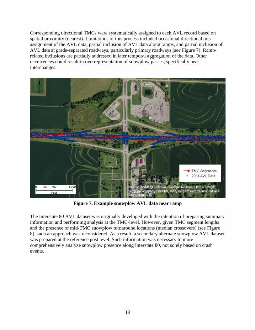
Corresponding directional TMCs were systematically assigned to each AVL record based on

spatial proximity (nearest). Limitations of this process included occasional directional mis-

assignment of the AVL data, partial inclusion of AVL data along ramps, and partial inclusion of

AVL data at grade-separated roadways, particularly primary roadways (see Figure 7). Ramp-

related inclusions are partially addressed in later temporal aggregation of the data. Other

occurrences could result in overrepresentation of snowplow passes, specifically near

interchanges.

Figure 7. Example snowplow AVL data near ramp

The Interstate 80 AVL dataset was originally developed with the intention of preparing summary

information and performing analysis at the TMC-level. However, given TMC segment lengths

and the presence of mid-TMC snowplow turnaround locations (median crossovers) (see Figure

8), such an approach was reconsidered. As a result, a secondary alternate snowplow AVL dataset

was prepared at the reference post level. Such information was necessary to more

comprehensively analyze snowplow presence along Interstate 80, not solely based on crash

events.

20

Figure 8. Example snowplow AVL data at mid-TMC, median crossover

Reference Posts

Unlike the “real-time” snowplow AVL data provided to the Iowa DOT (at the time of this study),

when changes occur or at a minimum interval of two minutes, the historic AVL data contains all

AVL readings (pings). Upon review of the temporal frequency of location reporting, and

snowplow speed while performing winter operations, a distance of 1,000 feet (upstream or

downstream) of reference post locations was determined appropriate for capturing AVL data of

interest. This distance was also used in a prior snowplow AVL project with the Office of

Maintenance. AVL data within 1,000 feet upstream or downstream of reference posts were

extracted from the previously created dataset, and the corresponding directional reference posts

were systematically assigned to each AVL record based on spatial proximity (nearest). Some of

previously noted limitations pertaining to AVL data along ramps and grade separations were

reduced, given the more infrequent coincidence with reference post locations. Table 3 presents

the resulting number of snowplow AVL records near reference posts.

Table 3. Snowplow AVL records near reference posts

Direction

Snowplow AVL Records

2013 2014

Eastbound 174,633 314,967

Westbound 183,252 332,070

21

While the AVL records presented in Table 3 were limited to those near reference posts, multiple

AVL pings may exist for the same snowplow pass. For example, for a given point in time, the

location for a single snowplow could have been captured multiple times within the 2,000 feet

considered. All captured records represent a single snowplow pass by the reference post;

inclusion of all records would result in an overestimation of snowplow operations. Therefore,

reduction of the reference post-based AVL data was necessary.

AVL records were aggregated into unique snowplow pass groups based on a combination of

unique plow number, heading, assigned directional reference post, and date/time. In this

instance, use of heading did not eliminate AVL records on proximate roadways. A 15-minute

interval was selected to conservatively address very low snowplow velocities as well as a

minimum interval for a return pass by the same snowplow in the same direction of travel.

Possible limitations of the data reduction approach include the following:

The distance of 1,000 feet (upstream or downstream) of reference post locations may not

capture all AVL records of interest, particularly in cases of GPS signal loss or transmission

issues.

The 15-minute interval may overrepresent snowplow passes when snowplow speeds are very

low due to traffic incidents.

Snowplow passes at/near interchanges may be overrepresented due to AVL data present

along ramps and grade-separated primary roadways. In future studies, additional

refinement/use of the heading attribute is recommended to limit any such possible over-

representations.

All snowplow attributes for the first temporal AVL record were retained for the pass group.

Based on the aggregation results and Office of Maintenance recommendations, the interval was

increased to 30 minutes in the crash-based analysis discussed later. Table 4 presents the resulting

estimated number of snowplow passes. In general, aggregation resulted in a reduction of

approximately 44 percent of records.

Table 4. Snowplow passes near reference posts

Low

Snowplow Passes

2013 2014

Eastbound 64,405 115,569

Westbound 65,668 117,905

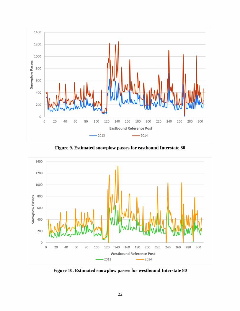
Figure 9 presents the estimated number of snowplow passes in 2013 for the eastbound reference

posts across the Interstate 80 corridor, while Figure 10 presents estimated number of snowplow

passes in 2014 for the westbound reference posts.

22

Figure 9. Estimated snowplow passes for eastbound Interstate 80

Figure 10. Estimated snowplow passes for westbound Interstate 80

0

200

400

600

800

1000

1200

1400

0 20 40 60 80 100 120 140 160 180 200 220 240 260 280 300

Sno

wp

low

Pas

ses

Eastbound Reference Post

2013 2014

0

200

400

600

800

1000

1200

1400

0 20 40 60 80 100 120 140 160 180 200 220 240 260 280 300

Sno

wp

low

Pas

ses

Westbound Reference Post

2013 2014

23

As discussed previously, a limited number of reference posts do not exist in both directions of

travel, which is evident by some zero pass frequencies. While estimated pass frequencies are

different for 2013 and 2014, their continuous pass lines are generally parallel throughout the

Interstate corridor, demonstrating the same relative frequencies. However, this is not always the

case, such as between reference posts 112 through 115. Highest frequency pass estimates

(peaks), in both directions of travel, are consistent throughout the Interstate 80 corridor and often

coincide with interchanges and median crossovers. This may represent a higher frequency of

snowplow turnarounds at these locations as well as partial inclusion of grade-separated

roadways. Other more continuous areas of higher relative passes typically represent urban areas

with more through lanes, interchanges, and higher traffic volumes. Figure 11 presents a

comparison of 2014 passes and 2014 passes normalized by the number of through lanes, which

reduces the magnitude of many of these higher relative pass areas.

Figure 11. Comparison of total and through lane snowplow passes for westbound Interstate

80

The reference post-based snowplow AVL pass estimates will be used, in part, in the negative

binomial regression models.

Crash-Based

To facilitate analysis at the crash level only, a slightly different approach was employed to

integrate snowplow AVL data with crashes. The Interstate 80 crash dataset was first separated

into four parts, based on direction of travel and year, and imported into the SQL Server database

in which the AVL data resided. Spatial temporal queries were then used to select all AVL

records of interest. Specifically, AVL records that satisfied the following criteria were selected:

0

200

400

600

800

1000

1200

1400

0 20 40 60 80 100 120 140 160 180 200 220 240 260 280 300

Sno

wp

low

Pas

ses

Westbound Reference Posts

2014 2014 Thru Lanes

24

Occurred in the same direction of travel as the crash

Located within a distance of 1,000 feet (upstream or downstream) from the crash

Occurred within two hours of the reported time of the crash

Unlike the AVL data extracted for integration at the TMC and reference post levels, no

additional conditional restrictions were applied (e.g., based on snowplow velocity or material

distribution), facilitating some additional analyses. New database tables were populated with the

resulting records, which included an additional attribute of the corresponding unique crash case

number. Because of the possible spatial and temporal proximity of crashes, a single AVL record

may be associated with multiple crashes.

Similar to the reference post-based AVL data, multiple AVL pings may exist for the same

snowplow pass. Therefore, AVL records were aggregated into unique snowplow pass groups

based on a combination of unique plow number, crash case number, direction of travel, and

date/time. Heading was removed from consideration to allow for possible further aggregation of

AVL data traversing both the mainline and a ramp; however, data along proximate other

roadways were not eliminated. Based on the reference post-based results and Office of

Maintenance recommendations, the time interval was expanded to 30 minutes (with a few minor

adjustments), which should still conservatively address low snowplow velocities as well as a

minimum interval for a return pass by the same snowplow in the same direction of travel.

Snowplow passes at a limited number of sites with turnaround times of less than 30 minutes may

potentially be underrepresented. As with the 15-minute interval, passes may potentially be

overrepresented when speeds are very low, due to traffic incidents. Passes may also be

overrepresented at/near interchanges. Descriptive attributes were calculated for each pass group,

such as minimum date/time, count of AVL records, average velocity, average heading and

distance between the crash and AVL ping.

Considering winter weather-related crashes only, Table 5 presents a comparison of the original

number of AVL records to the resulting estimated number of snowplow passes. Aggregation

resulted in a record reduction of more than 50 percent, which is slightly greater than that at the

reference post level. This may be due, in part, to a combination of relaxing the heading-related

conditions and increasing the time interval to 15 minutes.

Table 5. Snowplow AVL records and estimated passes near winter weather-related crashes

Type

Snowplow AVL Records

2013 2014

Original AVL 5,099 6,960

Estimated Passes 2,290 3,287

Traffic Speed Data

INRIX traffic speed data for calendar years 2013 and 2014 were provided to the Iowa DOT at

the TMC level. The speed data were derived from crowdsourced probe vehicles and were

25

provided at one-minute intervals. Attributes included current average speed, historic average

speed for the corresponding day of the week and time of day, reference (free flow) speed, and

confidence indicators pertaining to real-time speed. Temporal latency may exist with the real-

time speed data.

Using a combination of the reported winter crash date/time and the derived TMC of each

incident, INRIX speed data were independently identified for the 60 minutes before and after the

reported time of each winter crash. Occasionally, speed records were missing at the one-minute

interval. Additionally, the reported time of crash may represent an estimated time and not be

precise. Records applicable to multiple crashes were associated with all appropriate crashes.

Table 6 presents the number of traffic speed records by year and direction of travel.

Table 6. INRIX traffic speed records

Direction

Traffic Speed Records

2013 2014

Eastbound 51,214 57,258

Westbound 68,197 75,170

Corresponding unique crash case number and reported time of crash were assigned to each speed

record. The temporal difference in minutes from the reported crash time and each corresponding

speed record was then computed for analysis purposes.

Winter Maintenance Reports

Throughout the winter maintenance season, Iowa DOT maintenance crews record various

aspects of their operations efforts, weather conditions, road closures, and material usage in a

winter database. The corresponding reports are fairly high level, typically presented at the cost

center level. Some reports do, however, provide data based on roadway level of service (A, B, or

C) as well. Level A roads represent Interstates, Level B roads represent four-lane and major two-

lane highways, and Level C roads represent rural low traffic, two-lane highways. While cost

center and service level data (where available) allow for identification of a set of roadways, the

ability to conduct detailed analysis on specific roadways is limited. For the purpose of this

project, the crew and precipitation reports were of primary interest.

Crew Reports

Maintenance crew reports included attributes pertaining to event date, operation type, operation

beginning and ending times, time of near normal condition, and time of bare wheel path

condition. Reported maintenance operations included the following:

Anti-icing: Pre-storm operations

26

Phase 1: During-storm operations, from when precipitation is falling (or snow is blowing)

until near normal conditions are achieved on Level A roads

Frost run

Phase 2: Post-storm operations, such as clearing shoulders, pushing snow away from

guardrails, and benching back drifts. This may continue for a few days after a storm but is

typically completed during regular working hours.

Cost center, service level, and crew number are provided for each record. Therefore, records

could be limited to only the cost centers along Interstate 80 and Level A roads. As noted

previously, for some cost centers Interstate 80 is the only Level A road, while other cost centers

are responsible for additional Level A roads. For Level A roads within any given cost center,

maintenance operations may temporally coincide or overlap. In other words, multiple operations

records may exist for the same time period during a single day. An attempt was made to simplify

the data by aggregating records by cost center and date. Resulting attributes conveyed the

number of crews, type of operation(s) during the day, the earliest corresponding beginning time

for each operation, and estimated operation duration. Two limitations of the aggregated data

pertain primarily to the derived operation duration. Specifically, only the duration of an

operation for a given day is represented, beginning at midnight. This may represent a

continuation of the operation from the previous day. In those instances, the entire duration of an

operation related to a single winter weather event will not be represented. If an operation was

discontinued for a period of time during a given day, the derived duration may not account for

the temporal discontinuity, yielding an overestimated duration. The earliest time of that operation

is also conveyed.

Because the reference posts within each cost center were known, summary crew data were

presented both at the cost center and reference post level. These data were also spatially and

temporally associated with each crash, based on the cost center and event date.

Precipitation Reports

Precipitation reports include attributes pertaining to event date, precipitation type, start and end

times, and proximate RWIS-based air temperature, pavement temperature, wind direction, wind

velocity, and visibility. Reported precipitation types include the following:

Refreeze

Rain

Freezing rain

Sleet

Mixed precipitation

Snow

Blowing snow

Fog

Bridge frost

Road frost

27

None

Cost center is the only locational indicator in the precipitation records. Therefore, records could

simply be limited to cost centers along Interstate 80. Precipitation records may temporally

coincide or overlap, particularly while multiple precipitation types occur during a single day. An

attempt was made to simplify the data by aggregating records by cost center and date. Resulting

attributes conveyed the number of records for each precipitation type, the earliest corresponding

beginning time for each precipitation type, and estimated precipitation duration for each

precipitation type. Similar to the crew report summary, duration-related limitations may exist,

specifically related to precipitation types spanning days and temporal discontinuities.

Because the reference posts within each cost center were known, summary precipitation data

could be presented both at the cost center and reference post level. These data were also spatially

and temporally associated with each crash, based on the cost center and event date.

NWS COOP Stations

Data were collected from specific NWS COOP stations near Interstate 80 in and near Iowa. The

purpose was to determine the daily snowfall along the Interstate; it was decided that temperatures

and precipitation would not differ greatly from the nearby cities and the weather information

could be extrapolated from these sources. Table 7 lists the NWS COOP stations utilized for

snowfall data collection, and Figure 12 presents their locations along the corridor.

Table 7. NWS COOP stations along Interstate 80

City

Station

Code Station Name

Omaha NE6255 OMAHA EPPLEY AIRFIELD

Logan IA4894 LOGAN

Oakland IA6151 OAKLAND-2-E

Harlan IA3632 HARLAN

Atlantic IA0364 ATLANTIC-1-NE

Audubon IA0385 AUDUBON

Guthrie Center IA3509 GUTHRIE-CENTER

Greenfield IA3438 GREENFIELD

Winterset IA9132 WINTERSET

Des Moines Air. IA2203 Des Moines Airport

Ankeny IA0241 ANKENY-3-S

Iowa Average IA0000 Iowa Average

Newton IA5992 NEWTON

Grinnell IA3473 GRINNELL-3-SW

Williamsburg IA9067 WILLIAMSBURG

Iowa City IA4101 IOWA-CITY

Le Claire IA4705 Le Claire L&D 14

28

Figure 12. NWS COOP stations along Interstate 80

Snowfall amount was collected for each of these stations for all 365 days of each year, 2013 and

2014. Second, the snowfall data were queried to only include information for the winter months:

January 2013 to April 2013

October 2013 to December 2013

January 2014 to April 2014

October 2014 to December 2014.

The daily snowfall estimates were added to obtain the total yearly snowfall for each station. The

snowfall, in inches, was related to each reference post based on spatial proximity to each NWS

COOP station.

Roadway Weather Information Systems

RWIS stationary camera images and Wavetronix speed data were acquired for stations proximate

to selected winter weather-related crashes. Upon identifying crashes of potential interest,

corresponding data were downloaded from the Iowa Environmental Mesonet, which archives

much of the RWIS data. However, the fidelity of some of the data may be less than that

originally acquired. For example, the speed data were available at an interval of approximately

20 minutes.

29

Attributes for the speed dataset included RWIS station number, date/time, lane number, average

speed, average headway, volume (normal and long vehicles), and occupancy. Stationary images

from multiple cameras with different perspectives were also available at an interval of

approximately 20 minutes. For the purpose of this study, RWIS-based weather-related attributes

were not considered.

30

ANALYSIS

Interstate 80 Winter Crash Experience

Overview

During the winter maintenance periods of calendar years 2013 and 2014, 56 percent of the winter

crashes along the Interstate 80 corridor were weather related. To investigate whether this

proportion of weather-related crashes was generally representative of the corridor or simply an

anomaly, crash experience during the winter maintenance periods of calendar years 2011 through

2014 was analyzed, both for Interstate 80 and the Interstate system as a whole. During this

period, 46 percent of the winter crashes along Interstate 80 were weather related compared to

approximately 35 percent for the remaining Interstate system. Additionally, more than half (52

percent) of the winter weather-related crashes on the Interstate system occurred on Interstate 80,

while only 41 percent of the non-weather-related winter crashes occurred on Interstate 80. Even

though the proportion of weather-related crashes along Interstate 80 was lower during the

expanded analysis period (46 percent compared to 52 percent), winter weather-related crashes

still appear overrepresented along the corridor, especially when considering crash experience on

the system as a whole. A statistical test of proportions was conducted to identify possible

differences in crash characteristics.

Test of Proportions

For the winter maintenance periods of calendar years 2013 and 2014, statistical testing of the

difference between two proportions was performed to determine differences in crash

characteristics between weather-related and non-weather-related winter crashes along Interstate

80. To accomplish this, discrete pairs of weather- and non-weather-related crashes were

established, and the proportions of various crash characteristics (e.g., severity) within these pairs

computed. The differences between these pairs of proportions were statistically tested for

significance using the z-statistic for a standard normal random variable. The z-statistic was

applicable because the frequency of crashes for the tested characteristics in each sample was

greater than five, and the two population proportions being compared were independent (Moore

et al. 2003). Statistically significant differences within the samples suggest an increase of a

specific crash characteristic for the crash type.

To begin, the null hypothesis was defined as “the two population proportions are equal, or are

not different,” given by the following:

H0: p1 = p2. (1)

Therefore, the alternate hypothesis was defined as “the two population proportions are not equal,

or are different,” i.e.,

H1: p1 ≠ p2 (2)

31

where p1 represents the first proportion being tested and p2 represents the second proportion.

A 95% level of confidence (significance level of 0.05) was selected, and the difference between

the sample proportions computed:

|p1 - p2| (3)

Then, the weighted average of the two sample proportions was computed:

𝑝 =𝑛1𝑝1+𝑛2𝑝2

𝑛1+𝑛2 (4)

where n1 and n2 are the respective number of observations sampled from the two populations.

The estimated standard error of the difference between proportions was calculated as follows:

sp1-p2=√

p(1-p)

n1+

p(1-p)

n2 (5)

The z-statistic was computed by the following general formula:

𝑧 =|𝑝1−𝑝2|

𝑠𝑝1−𝑝2 (6)

The probability of obtaining a difference between the population proportions as large as or larger

than the difference observed in the experiment, i.e., probability value or p-value, was determined

within Microsoft Excel (Lane 2009). The basic formula can be expressed as follows:

=IF(z-stat<0,2*NORMDIST(z-stat,0,1,1),2*(1-NORMDIST(z-stat,0,1,1))) (7)

where z-stat represents the address of the cell containing the z-statistic value (Barreto and

Howland 2008).

Last, the probability value was compared to the significance level of 0.05. If the probability

value was less than or equal to the significance level, the difference tested was significant, and

the null hypothesis was rejected. The tests were also conducted using a 90% level of confidence,

which would yield less significant results.

Results

Weather-related crashes were lower severity, with a statistically significant lower proportion of

fatal and possible/unknown injury crashes (p < 0.05) and higher proportion of property damage

32

only crashes (p < 0.05). In general, all winter crashes were lower severity, with only 17 percent

of weather-related crashes and approximately 24 percent of non-weather-related crashes resulting

in a fatality or injury. Severe crashes, resulting in a fatality or serious injury, only represented 1.3

percent and 2.5 percent of crashes, respectively.

Weather-related crashes were proportionally higher (p < 0.05) during the morning hours of 8:00

a.m. to 11:00 a.m. More than twice as many (nearly 23 percent) of weather-related crashes

occurred during these hours, compared to 10 percent of non-weather-related crashes. Conversely,

non-weather-related crashes were proportionally higher (p < 0.05) during several hours,

particularly 4:00 p.m. until 7:00 p.m. During these hours, 21 percent of non-weather-related

crashes occurred compared to 12 percent of weather-related crashes. The time of day results

observed on Interstate 80 are generally consistent with the Interstate system as a whole.

Specifically, weather-related crashes occur more frequently during morning commute hours, and

non-weather-related crashes occur more frequently during afternoon commute hours. This may

be due, in part, to motorists’ real or perceived lack of flexibility with respect to arrival to work or

school, awareness of conditions, and general weather patterns.

Collisions with many fixed objects—concrete barrier, raised median, ditch/embankment,

guardrail, sign post, and other fixed object—were proportionally higher (p < 0.05) for weather-

related crashes, with concrete barrier and guardrail collisions representing nearly 36 percent of

the crashes, compared to approximately 15 percent of non-weather-related crashes. No weather-

related crashes involved a collision with an animal, which represent 16 percent of non-weather-

related crashes (p < 0.05). Additionally, the proportion of non-weather-related crashes involving

a collision with a vehicle was comparatively higher (p < 0.05), 43 to 29 percent, for non-

weather-related crashes. These first harmful events are further supported by the proportional

differences (p < 0.05) in single- and multiple-vehicle winter crashes as well as manners of

crash/collision. Nearly 67 percent of weather-related crashes are single-vehicle, non-collision

crashes, while 52 percent of non-weather-related crashes involve a single vehicle. Approximately

26 percent of non-weather-related crashes are rear-end, compared to 14 percent of weather-

related crashes (p < 0.05).

Proportions of 17 of the 25 possible derived crash major causes were significantly different (p <

0.05). The greatest proportional differences for non-weather-related proportions were animal

crashes (17 percent greater) and followed too close (10 percent greater). Conversely, the greatest

proportional difference for weather-related crashes (41 percent) was observed for driving too fast

for conditions.

The proportion of crashes by direction of travel along Interstate 80 was not significantly different

for weather- and non-weather-related crashes. Weather-related crashes were proportionally

greater for higher speed portions of Interstate 80 but to a lesser significance level (p < 0.1).

33

Maintenance Operations

Crew and Precipitation Reports

For the winter maintenance periods of calendar years 2013 and 2014, maintenance crew report

records and winter weather-related crashes were integrated based on cost center and date.

Through this integration, the general relationship between Phase 1 (during storm) operations and

crash experience was assessed, with the primary objective of determining crash experience

during days with and without Phase 1 operations. Actual duration of Phase 1 operations was not

taken into consideration.

Figure 13 and Figure 14 for 2013 and 2014, respectively, present the number of days of Phase 1

operations by cost center, as well as the corresponding number of days with at least one crash.

For purposes of this report, cost centers are not explicitly identified and are represented by a

single character.

Figure 13. Phase 1 operations (2013)

0

10

20

30

40

50

60

A B C D E F G H I J K L M N O P

Day

s

Cost Center

2013 Phase 1 Operations 2013 Phase 1 Operations w/ Crashes

34

Figure 14. Phase 1 operations (2014)

For all maintenance garages responsible for the Interstate 80 corridor, approximately 70 percent

of the days with Phase 1 operations had no winter weather-related crashes. At the garage level,

the highest percentage of Phase 1 operation days with a crash was approximately 50 percent.

During the analysis period, only 22 winter weather-related crashes (16 in 2013 and 6 in 2014)

occurred on days in which no Phase 1 operations were reported. Both the low percentage of

Phase 1 days with weather-related crashes and the limited number of weather-related crashes

reported on days with no Phase 1 operations appears to broadly suggest that Phase 1 operations

are successful and present during appropriate times.

Figure 15 presents a comparison of the total number of days on which a winter weather-related

crash occurred and the total number of days with multiple weather-related crashes.

0

10

20

30

40

50

60

70

A B C D E F G H I J K L M N O P

Day

s

Cost Center

2014 Phase 1 Operations 2014 Phase 1 Operations w/ Crashes

35

Figure 15. Winter weather-related crash days (2013, 2014)

Overall, multiple crashes occurred during more than half of the days, with multiple crashes

occurring on nearly 70 percent of the days within two cost centers. This appears to suggest that a

limited number of weather events may contribute more greatly to crash experiences, which may

be affected by winter weather event duration, timing, and intensity. For example, exposure is

increased during longer storm events as well as those occurring during peak travel hours.

As was discussed previously, winter weather-related crashes are proportionally higher during the

morning hours, particularly during the morning traffic peak hours. Figure 16 presents a

distribution of crashes by hour of day.

Figure 16. Winter weather-related temporal distribution

0

5

10

15

20

25

30

35

40

45

50

A B C D E F G H I J K L M N O P

Day

s

Cost Center

Phase 1 Operations w/ Crashes Phase 1 Operations w/ Mult. Crashes

0

10

20

30

40

50

60

0 1 2 3 4 5 6 7 8 9 10 11 12 13 14 15 16 17 18 19 20 21 22 23

Win

ter

Wea

ther

-rel

ated

Cra

shes

Hour of Day

2013 2014

36

Forty percent of crashes occurred during the six hours from 6:00 to 11:00 a.m. Motorists’ real or

perceived lack of flexibility with respect to arrival to work or school, awareness of conditions,

and general weather patterns may be possible factors affecting morning crash frequency.

Possible weather pattern-related impacts may be further investigated through maintenance crew

and precipitation reports.

Figure 17 presents the frequency distribution of weather-related crashes based on the beginning

hour of Phase 1 operations.

Figure 17. Beginning hour of Phase 1 operations, 2013 and 2014

Figure 17 is not dependent on crash time of day but simply on cost center and crash date. For

example, a crash occurring at 8:30 a.m. on a day during which Phase 1 operations began at 4:00

a.m. is represented in the “4” hour. More than 50 percent of weather-related crashes occurred

when Phase 1 operations were reported before 7:00 a.m. and increased to 77 percent before noon.

The significant peak at midnight may represent, in part, existing maintenance reporting

protocols, such as a continuation of Phase 1 operations from the previous day or a shift change.

Regardless, initiation or continuation of Phase 1 operations are prominent during the morning

hours on days with winter weather-related crashes.

The distribution of weather-related crashes, based on the beginning hour of snow (Figure 18), is

generally consistent with the beginning hour of Phase 1 operations (Figure 17).

0

20

40

60

80

100

120

140

160

180

0 1 2 3 4 5 6 7 8 9 10 11 12 13 14 15 16 17 18 19 20 21 22 23 NR

Win

ter

Wea

ther

-rel

ated

Cra

shes

Begin Hour of Phase 1 Operations

2013 2014

37

Figure 18. Beginning hour of precipitation (snow), 2013 and 2014

A greater frequency of crashes with no corresponding records, i.e., reported snow on the day of

the weather-related crash, is also apparent. This may be due to the presence of other types of

precipitation as well as other conditions, such as blowing snow, warranting for Phase 1

operations. Existing reporting protocols may also explain the higher frequency during the

midnight hour. In general, on days with winter weather-related crashes, snow has fallen or has

begun to fall during the morning. No comparison was made to days with no weather-related

crashes.

Figure 19 presents the frequency of winter weather-related crashes based on the difference in

hours between the reported initiation of Phase 1 operations and crash occurrence.

0

20

40

60

80

100

120

140

160

0 1 2 3 4 5 6 7 8 9 10 11 12 13 14 15 16 17 18 19 20 21 22 23 NR

Win

ter

Wea

ther

-rel

ated

Cra

shes

Begin Hour of Snow

2013 2014

38

Figure 19. Phase 1, crash time comparison, 2013 and 2014

Figure 19 reveals that the majority of weather-related crashes occur within several hours after the

beginning of Phase 1 operations. Seven percent of the crashes occur within the same hour, while

an additional 20 percent occur within the subsequent two hours. More than 50 percent of the

crashes occur within the same hour and subsequent five hours. These results are somewhat

intuitive given the definition of Phase 1 operations on Interstates, i.e., during-storm operations,

from when precipitation is falling (or snow is blowing) until near normal conditions are achieved

on Level A roads. Only 3 percent of crashes occurred before the reported beginning hour of

Phase 1 operations.

The decrease in in crash frequency after the tenth hour of Phase 1 operations may be explained

by reduced winter weather event intensity over time as well as the more sustained impacts of

Phase 1 maintenance operations on road conditions. Furthermore, the hour of day during which

Phase 1 operations begin may impact the observed temporal crash patterns. Higher percentages

of both Phase 1 operations and weather-related crashes are observed during the morning hours.

Snowplow AVL: Crash-Based

Through the previously discussed spatial and temporal integration of winter weather-related

crashes and snowplow AVL data, temporal relationships between snowplow pass(es) and crash

occurrence may be explored. From an operational perspective, such information may be useful in

evaluating maintenance policies on Level A roadways as well as observed pass frequencies with

respect to crash experience. A limitation of this approach is that comprehensive maintenance

operations, independent of crash experience, are not taken into consideration. No basis for

comparison exists for snowplow pass intervals, at given crash locations, during “no crash” winter

weather events. Therefore, assessment of whether crash-based snowplow intervals are

representative or atypical is not possible. The statistical analysis presented in the next section

0

10

20

30

40

50

60

70

-2+

-1 0 1 2 3 4 5 6 7 8 9 10 11 12 13 14 15 16 17 18 19 20 21 22 23 24NR

Win

ter

Wea

ther

-rel

ated

Cra

shes

Hours between Phase 1 Operations and Crash

2013 2014

39

somewhat addresses this by considering comprehensive, reference post-based snowplow pass

and crash frequency, while not evaluating snowplow pass time interval.

Another limitation of the previously discussed approach is that it doesn’t take into consideration

the unique weather conditions of each event. Specifically, weather conditions, such as wind

velocity and direction, surface and atmospheric temperatures, precipitation type and intensity,

and surface conditions, are likely differ to some extent among all weather events. Such

differences may impact maintenance operations as well as the general traffic conditions within

which the snowplows must operate. For example, low traffic speeds and incidents may impact

snowplow pass frequency.

While impacts may be minor, other possible limitations of data analysis and interpretation may

include the following:

No absolute confirmation exists that snowplows were engaged in maintenance operations.

Snowplow passes may be overrepresented in low traffic speed conditions and when crashes

were located at/near an interchange.

Snowplow AVL data may potentially be incomplete, due to communication or acquisition

issues. Occurrence, if any, and frequency cannot be identified and quantified.

Spatial and temporal aggregation assumptions with respect to AVL pings and crash time and

location may influence snowplow pass identification.

Lane position of both the crash and snowplow(s) are unknown.

The reported crash time may be approximate.

Because of presumed incomplete AVL data during February, March, and April of 2013, these

months were removed from the analysis. For all other months during the winter maintenance

analysis period, the total frequency of snowplow passes, within two hours before and after the

reported crash time, were calculated for each crash. Due to possible temporal and spatial

proximity of multiple crashes, a single snowplow pass may be associated with multiple crashes.

In some cases, no snowplow passes were identified within two hours before and/or after a

reported crash time.

The time intervals, in minutes, between snowplow passes before and after each reported crash

time were also calculated for each snowplow pass. These data were then used to determine the

following time intervals for each crash: 1) between the most recent before (or last before)

snowplow pass and the reported crash time, 2) between the reported crash time and the first after

snowplow pass. Note that these passes may be by different plows, and if multiple snowplow

passes occurred at approximately the same time, only the last before and first after times were

identified. However, all passes were recorded in the pass frequency calculations. The following

series of figures and tables present crash experience with respect to these last before and first

after snowplow pass time intervals.

In both Figure 20 and Figure 21, crashes occurring within the winter maintenance periods of

2013 (excluding February through April) and 2014 are considered together. Figure 20 presents

40

the frequency of winter weather-related crashes with respect to the elapsed time, in minutes,

since the last snowplow pass before the crash, i.e. the most recent or last before pass.

Figure 20. Last before snowplow pass, crash time interval

Crashes with no snowplow passes within two hours before the crash were excluded from Figure

20. Time -120 represents two hours prior to the reported crash, while time 0 represents the

reported time of the crash. Crashes are clearly more frequent as more time has elapsed since the

last before snowplow pass.

Figure 21 presents the elapsed time, in minutes, between the crash and the first snowplow pass

after the crash (or first after pass).

0

2

4

6

8

10

12

14

16

18

-12

0

-11

5

-11

0

-10

5

-10

0

-95

-90

-85

-80

-75

-70

-65

-60

-55

-50

-45

-40

-35

-30

-25

-20

-15

-10 -5 0

Win

ter

Wea

ther

-rel

ated

Cra

shes

Last Before Plow Pass (minutes)

2013 2014

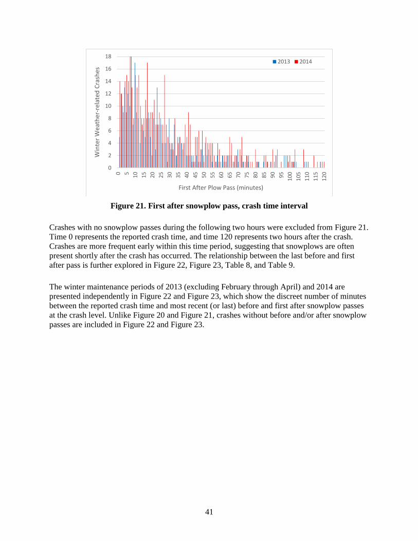
41

Figure 21. First after snowplow pass, crash time interval

Crashes with no snowplow passes during the following two hours were excluded from Figure 21.

Time 0 represents the reported crash time, and time 120 represents two hours after the crash.

Crashes are more frequent early within this time period, suggesting that snowplows are often

present shortly after the crash has occurred. The relationship between the last before and first

after pass is further explored in Figure 22, Figure 23, Table 8, and Table 9.

The winter maintenance periods of 2013 (excluding February through April) and 2014 are

presented independently in Figure 22 and Figure 23, which show the discreet number of minutes

between the reported crash time and most recent (or last) before and first after snowplow passes

at the crash level. Unlike Figure 20 and Figure 21, crashes without before and/or after snowplow

passes are included in Figure 22 and Figure 23.

0

2

4

6

8

10

12

14

16

18

0 5

10

15

20

25

30

35

40

45

50

55

60

65

70

75

80

85

90

95

10

0

10

5

11

0

11

5

12

0

Win

ter

Wea

ther

-rel

ated

Cra

shes

First After Plow Pass (minutes)

2013 2014

42

Figure 22. Snowplow pass, crash time interval (2013)

Figure 23. Snowplow pass, crash time interval (2014)

Each point conveys the elapsed time, in minutes, between when the crash occurred and: 1) the

last snowplow pass before the crash (last before) and 2) the corresponding first snowplow pass

after the crash (first after). For example, a point located at -100, 20 indicates that a snowplow last

passed the crash location 100 minutes before the crash, and the next snowplow passed 20

minutes after the crash. The last before and first after snowplows may be different.

The cluster of points in the lower left-hand corner of both figures indicates a greater time

difference between the last (before) snowplow passes and subsequent (first) after passes, which

comparatively occur more recently after a crash. Furthermore, the time difference between the

43

before and after snowplow passes in these clusters falls within the general operational

expectations of a Level A roadway, i.e., an approximately two-hour snowplow return time. This

may suggest that more crashes occur as the time increases since the last snowplow pass.

Alternatively, it may simply reflect the presence of a snowplow approximately every two hours

based on the aforementioned Level A operational expectations.

The frequency of no observed snowplow passes (NR) is higher for last before the crash

compared to the frequency for first after the crash. If the snowplow AVL data are assumed to be

mostly complete, this may suggest that crashes are occurring early in winter weather events,

possibly before maintenance operations have been fully initiated or mobilized. On the other

hand, if the snowplow AVL data are partially incomplete, this may simply indicate missing data.

Table 8 and Table 9 present the data from Figure 22 and Figure 23 in a tabular format.

Specifically, crash frequency and corresponding percentages are presented, in 30-minute

intervals, for the most recent (last) before and first after snowplow passes.

Table 8. Snowplow pass, crash time interval (2013)

Last

Before

Pass

(Minutes)

First After Pass (Minutes)

Total < 30 30–60 60–90 90–120 120+ NR

# % # % # % # % # % # % # %

< 30 20 5 7 2 4 1 9 2 1 0 41 10

30–60 19 5 7 2 7 2 3 1 3 1 39 10

60–90 36 9 18 5 2 1 2 1 4 1 62 16

90–120 108 28 29 7 5 1 1 0 7 2 150 38

120+ 3 1 2 1 2 1 7 2

NR 43 11 17 4 8 2 3 1 1 0 22 6 93 24

Total 229 58 80 20 28 7 18 5 1 0 37 9 392 100

NR = no observed snowplow passes

Table 9. Snowplow pass, crash time interval (2014)

Last

Before

Pass

(Minutes)

First After Pass (Minutes)

Total < 30 30–60 60–90 90–120 120+ NR

# % # % # % # % # % # % # %

< 30 28 5 15 3 5 1 3 1 3 1 54 9

30–60 39 7 17 3 6 1 2 0 1 0 65 11

60–90 59 10 33 6 8 1 5 1 8 1 113 19

90–120 126 21 37 6 16 3 11 2 10 2 200 34

120+ 13 2 2 0 1 0 16 3

NR 49 8 21 4 14 2 2 0 1 0 55 9 142 24

Total 314 53 125 21 50 8 23 4 1 0 77 13 590 100

NR = no observed snowplow passes

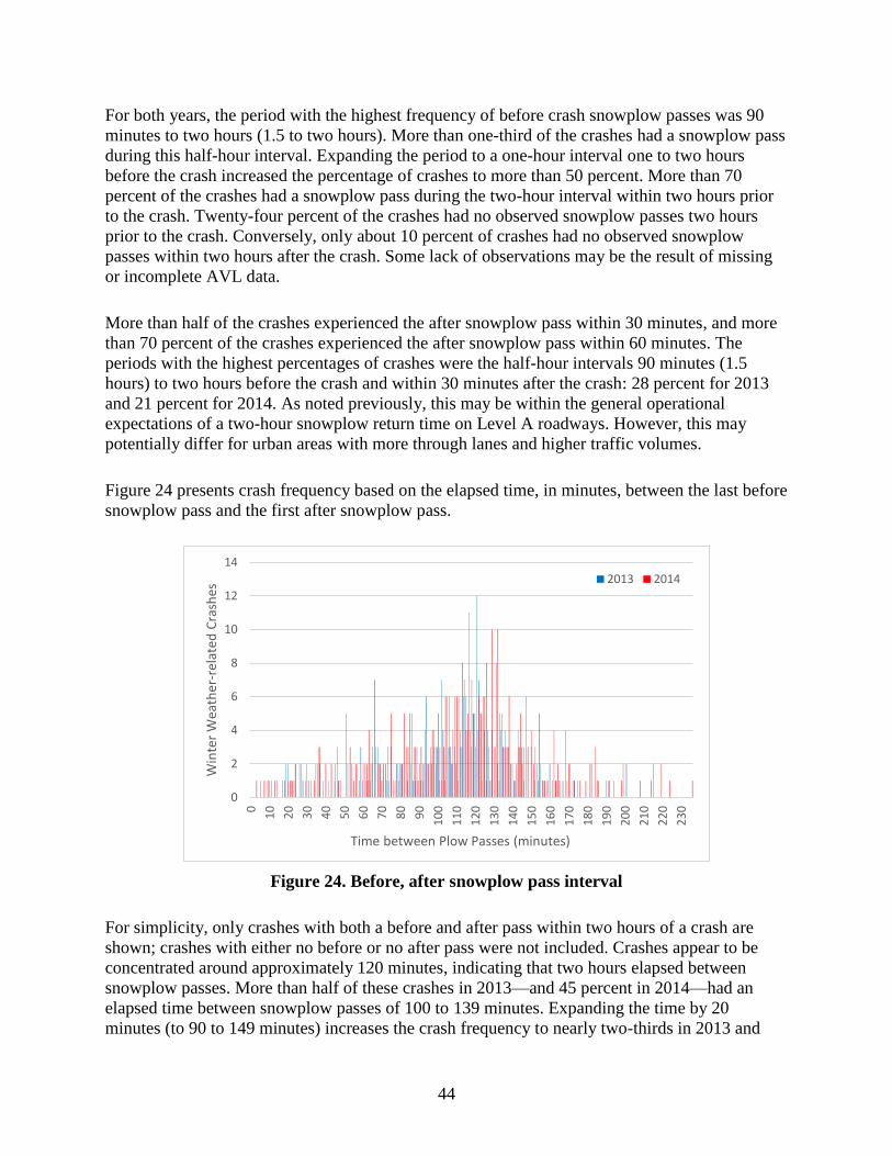
44

For both years, the period with the highest frequency of before crash snowplow passes was 90

minutes to two hours (1.5 to two hours). More than one-third of the crashes had a snowplow pass

during this half-hour interval. Expanding the period to a one-hour interval one to two hours

before the crash increased the percentage of crashes to more than 50 percent. More than 70

percent of the crashes had a snowplow pass during the two-hour interval within two hours prior

to the crash. Twenty-four percent of the crashes had no observed snowplow passes two hours

prior to the crash. Conversely, only about 10 percent of crashes had no observed snowplow

passes within two hours after the crash. Some lack of observations may be the result of missing

or incomplete AVL data.

More than half of the crashes experienced the after snowplow pass within 30 minutes, and more

than 70 percent of the crashes experienced the after snowplow pass within 60 minutes. The

periods with the highest percentages of crashes were the half-hour intervals 90 minutes (1.5

hours) to two hours before the crash and within 30 minutes after the crash: 28 percent for 2013

and 21 percent for 2014. As noted previously, this may be within the general operational

expectations of a two-hour snowplow return time on Level A roadways. However, this may

potentially differ for urban areas with more through lanes and higher traffic volumes.

Figure 24 presents crash frequency based on the elapsed time, in minutes, between the last before

snowplow pass and the first after snowplow pass.

Figure 24. Before, after snowplow pass interval

For simplicity, only crashes with both a before and after pass within two hours of a crash are

shown; crashes with either no before or no after pass were not included. Crashes appear to be

concentrated around approximately 120 minutes, indicating that two hours elapsed between

snowplow passes. More than half of these crashes in 2013—and 45 percent in 2014—had an

elapsed time between snowplow passes of 100 to 139 minutes. Expanding the time by 20

minutes (to 90 to 149 minutes) increases the crash frequency to nearly two-thirds in 2013 and

0

2

4

6

8

10

12

14

0

10

20

30

40

50

60

70

80

90

10

0

11

0

12

0

13

0

14

0

15

0

16

0

17

0

18

0

19

0

20

0

21

0

22

0

23

0

Win

ter

Wea

ther

-rel

ated

Cra

shes

Time between Plow Passes (minutes)

2013 2014

45

nearly 60 percent in 2014. As discussed previously, these time intervals fall within the general

operational expectations of a Level A roadway, i.e., an approximately two-hour snowplow return

time. This may suggest that more crashes occur as the time increases since the last snowplow

pass or reflect the presence of a snowplow approximately every two hours.

In general, the summary tables and figures represent a macro-level analysis of estimated

snowplow passes and appear to further confirm that more crashes occur as the time since the last

snowplow pass increases, and approximately half as many crashes have no before plow passes

compared to after plow passes. These observations do not take into consideration other factors,

such as overall traffic speed, congestion, subsequent delays and event intensity, which may also

impact snowplow operations. They also do not take into consideration possible inaccuracies in

reported crash times, which could influence whether a snowplow pass is considered “before” or

“after” the crash. Micro-level analysis, which was out of the scope of this project, could be

explored to quantify the possible impacts of these extraneous factors and the previously

discussed limitations. For example, consistency in the pass time interval and frequency could be

assessed for proximate locations at a given time period.

Table 10 and Table 11 present the estimated number of snowplow passes within two hours

before and after a crash.

Table 10. Snowplow pass frequency (2013)

Before

Pass

Frequency

After Pass Frequency

Total 1–2 3–4 5–6 > 6 NR

# % # % # % # % # % # %

1–2 57 15 49 13 18 5 7 2 9 2 140 36

3–4 20 5 37 9 19 5 10 3 5 1 91 23

5–6 6 2 16 4 13 3 9 2 1 0 45 11

> 6 12 3 6 2 5 1 23 6

NR 43 11 21 5 5 1 2 1 22 6 93 24

Total 126 32 135 34 61 16 33 8 37 9 392 100

NR = no observed snowplow passes

Table 11. Snowplow pass frequency (2014)

Before

Pass

Frequency

After Pass Frequency

Total 1–2 3–4 5–6 > 6 NR

# % # % # % # % # % # %

1–2 93 16 57 10 26 4 7 1 18 3 201 34

3–4 48 8 53 9 36 6 18 3 3 1 158 27

5–6 4 1 30 5 17 3 10 2 1 0 62 11

> 6 3 1 5 1 6 1 13 2 27 5

NR 43 7 28 5 15 3 1 0 55 9 142 24

Total 191 32 173 29 100 17 49 8 77 13 590 100

NR = no observed snowplow passes

46

The frequency of snowplow passes does not take into consideration the number of lanes at the

crash site; therefore, more passes would be expected as the number of lanes increases. Over one-

third of the crashes experienced one or two snowplow passes both before and after the crash. Not

shown in the tables is that two passes occurred more frequently than one pass, i.e., greater than

60 percent for both before and after passes.

Expanding the frequency of snowplow passes by one to four increases the percentage of crashes

to greater than 60 percent. Approximately 70 percent of the crashes had one to six snowplow

passes before the crash, while 80 percent of the crashes had one to six snowplow passes after the

crash. The high frequency of snowplow passes during the two hours before and after the crash

may suggest that crashes are occurring early in the weather event as well as during periods of

high snowplow activity. Additionally, since snowplow passes and crashes were integrated based

on direction of travel, the high frequencies may indicate that multiple lanes were being plowed

during this period. More than 60 percent of the crashes had at least two “before” snowplow

passes, and more than 70 percent had at least two “after” passes.

Due to incomplete or inaccurate front plow position data, the previous figures and tables were

based on assumptions made regarding snowplow maintenance operations. To investigate

potential validity, as well as the snowplow speeds and pass frequency with respect to the

weather-related crash time, Figure 25 and Figure 26 were prepared.

Figure 25. Snowplow velocity and passes, speed limit less than 70 mph

0

20

40

60

80

100

120

140

24

26

28

30

32

34

36

-12

0

-11

0

-10

0

-90

-80

-70

-60

-50

-40

-30

-20

-10 0

10

20

30

40

50

60

70

80

90

10

0

11

0

12

0

Plo

w P

asse

s

Vel

oci

ty (

mp

h)

Minutes Before/After Crash

Plow Passes Ave. Plow Velocity

47

Figure 26. Snowplow velocity and passes, 70 mph speed limit

Figure 25 presents snowplow data for roadways with a speed limit less than 70 mph; Figure 26

presents data for roadways with a speed limit of 70 mph. Both figures present both 2013

(excluding February through April) and 2014 crash numbers. In each figure, the horizontal axis

represents difference in time (in minutes), two hours before and after a winter weather-related

crash. Time 0 is the reported time of the crash. The primary vertical axis represents a five minute

moving average of snowplow velocity. These data are presented as red and blue lines,

respectively. The secondary vertical axis represents the number of snowplow passes and is

presented as gray bars.

While a five-minute moving average was employed to reduce the impacts of snowplow velocity

variations, variations are still apparent both before and after the crash. Snowplow velocities are

generally higher as the time prior to the crash is increased. Pre-crash velocities are consistent

with those of snowplows actively performing maintenance, whether plowing or distributing

liquid/granular material. Velocities rapidly decrease immediately prior to the crash and are

lowest within approximately 30 minutes after the crash. Velocities during this period may be

lower for several reasons, such as traffic speeds resulting from the crash itself or poor

weather/surface conditions. Average velocities gradually increase after the crash, not quite

reaching pre-crash averages. Velocities are generally consistent between roadways possessing

different speed limits but are somewhat lower for roadways with a speed limit less than 70 mph.

Variation also exists in the frequency of snowplow passes. In general, fewer passes occur prior to

the crash. The average snowplow pass frequency is higher following the crash, with the highest

pass frequencies occurring immediately following the reported time of the crash. The peak is

more pronounced for the lower speed roadways, where higher frequencies exist both before and

after the crash. Higher frequencies are sustained longer for the higher speed roadways, with a

gradual increase prior to the crash. These observations may be impacted by possible inaccuracies

in reported crash times.

0

20

40

60

80

100

24

26

28

30

32

34

36

-12

0

-11

0

-10

0

-90

-80

-70

-60

-50

-40

-30

-20

-10 0

10

20

30

40

50

60

70

80

90

10

0

11

0

12

0

Plo

w P

asse

s

Vel

oci

ty (

mp

h)

Minutes Before/After Crash

Plow Passes Ave. Plow Velocity

48

Finally, more snowplow passes were observed on roadways with a speed limit less than 70 mph

compared to those with a speed limit of 70 mph, approximately 30 percent in 2013 and 10

percent in 2014. While these sections include less than one-quarter of corridor lane miles, they

are responsible for nearly one-third of the corridor vehicle miles traveled. They are

predominantly urban, having on average one additional lane in each direction of travel as well as

more interchanges compared to the higher speed sections. Their weighted AADT is also nearly

twice that of the 70 mile per hour sections. Approximately 40 percent of the winter weather-

related crashes occurred on the sections with a speed limit less than 70 mile per hour sections,

compared to 60 percent on the 70 mile per hour roadways.

In order to most effectively use any of the aforementioned information to assess maintenance

operations, a better understanding of typical, non-crash conditions may be necessary. Integration

of additional data may also be beneficial, including traffic flow, detailed weather conditions, and

surface conditions. A following section introduces use of snowplow images to evaluate possible

weather, surface, and traffic-related crash conditions. Additional datasets, such as maintenance

crew reports and INRIX traffic speed data, are integrated to serve as supplements to enhance

incident-level analysis.

Snowplow AVL: Reference Post-Based

Through the previously discussed spatial and temporal integration of winter crashes (non-

weather and weather-related), roadway characteristics, traffic volume and mix, snowfall, and

estimated snowplow AVL data at the reference post level, an assessment of safety impacts of

roadway maintenance during winter conditions was conducted. Table 12 provides a summary of

the descriptive statistics for the variables collected and utilized in this assessment.

49

Table 12. Descriptive statistics

Parameter Average Std. Dev. Min Max

Direction (0-East, 1-West) 0.50 0.50 0.00 1.00

Yearly plow passes 298.78 184.87 0.00 1323.00

Directional AADT 15763.92 8103.60 9000.00 68200.00

Truck Ratio 0.32 0.06 0.12 0.42

Yearly snowfall (in.) 28.35 11.18 3.00 52.80

Outside shoulder width (ft) 10.03 0.75 3.00 14.00

Outside shoulder rumble strip presence 0.61 0.49 0.00 1.00

Inside shoulder width (ft) 6.54 1.68 3.00 15.00

Inside rumble strip presence 0.92 0.27 0.00 1.00

Median width (ft) 43.43 75.86 0.00 1100.39

Number of through lanes 2.12 0.37 2.00 4.00

Number of exit lanes 0.03 0.18 0.00 2.00

Number of entrance lanes 0.05 0.22 0.00 1.00

Total number of lanes 2.20 0.48 2.00 4.00

Entrance Ramp Presence 0.33 0.47 0.00 1.00

Exit Ramp Presence 0.32 0.47 0.00 1.00

Ramp Count 0.66 0.85 0.00 4.00

Speed Limit 68.90 2.51 55.00 70.00

Non-winter weather crashes 0.78 1.16 0.00 10.00

Winter weather crashes 1.00 1.50 0.00 11.00

Total Crashes 1.78 2.12 0.00 14.00

The directional AADT is quite large, as is expected for a major Interstate that runs east and west

through Iowa and carries a large truck volume percentage; on average, one-third of the traffic is

composed of large trucks. The average snowfall per reference post among the two winters was

28 inches, and the average snowplow pass frequency per reference post was almost 300 passes.

Additionally, there are more winter weather-related crashes than non-winter weather-related

crashes during the winter periods. For all three categories of crashes, winter weather-related,

non-winter weather-related, and total crashes, the standard deviation is larger than the mean

value, which indicates an over dispersion of the crash data.

In addition to the variables presented in Table 12, the data also have several grouping features

that are presented in Table 13. Each of these features could potentially be utilized as a grouping

variable for a random effect model, the results of which are discussed later.

50

Table 13. Groups within data

Group Number

Years 2

Sites 600

Reference Posts 303

Weather Stations 17

Statistical Models

Once the database was assembled, the safety performance function was estimated for winter

weather-related crashes as a function of traffic volume, roadway geometric variables, snowfall,

and snowplow passes for each reference post.

One of the common frameworks for crash data modeling is the Poisson model. The probability of

a segment or intersection i experiencing yi crashes during a specific period, in the structural form

shown in Equation 8.

𝑃(𝑦𝑖) =𝐸𝑋𝑃(−𝜆𝑖)𝜆𝑖

𝑦𝑖

𝑦𝑖! (8)

where λi is the Poisson parameter for segment i, which is equal to the segment’s expected

number of crashes during the analysis period, E[yi]. Poisson regression models are estimated by

specifying the Poisson parameter λi as a function of explanatory variables. The most common

functional form for the Poisson parameter is shown in Equation 9.

λi = EXP(βXi) (9)

where Xi is a vector of explanatory variables and β is a vector of estimable parameters. However,

all types of crash data collected for this study were shown to be over dispersed, where the

variance is larger or smaller than the sample mean. To accommodate for the over dispersion of

crash data, a negative binomial regression model was initially utilized. The negative binomial

model is derived by rewriting this Poisson parameter for each segment i, as shown in Equation

10.

λi = EXP(βXi + εi) (10)

where EXP(εi) is a gamma-distributed error term with mean 1 and variance α. The addition of

this term allows the variance to differ from the mean, as shown in Equation 11.

VAR[yi] = E[yi] + αE[yi]2 (11)

51

The α term is also known as the over dispersion parameter, which is reflective of the additional

variation in crash counts beyond the Poisson model (where α is assumed to equal zero).

Additionally, to account for temporal correlation among the observations for each reference post,

a random effects framework was utilized instead. This model allows for the constant term to vary

across locations (study sites), as shown in Equation 12.

𝛽𝑖 = 𝛽 + 𝜔𝑖 (12)

where the i subscript indexes a specific road segment and 𝜔𝑖 is a random error term that is

assumed to follow a specific distribution. The error term is assumed to follow a normal

distribution, with a mean of zero and variance to be estimated as a model parameter, which is

allowed to vary across mile posts.

Results

In order to gain a fundamental understanding of the data, several plots were developed. When

examining count data, such as traffic crash frequency, it is critical to establish an appropriate

measure of exposure. In crash frequency models, traffic volume in terms of vehicles per day is

typically used as the exposure measure. In these data, each segment is one mile long, so there is

no need to control for length. Figure 27 presents winter weather crashes versus traffic volume. In

order to clearly illustrate the relationship between traffic volume and crashes, a line based on

log-transformed volume has been fitted to the data. As expected, traffic volume and crash

frequency are directly correlated.

Figure 27. Winter weather crashes versus directional traffic volume

y = 1.9902ln(x) - 18.07

0

2

4

6

8

10

12

0 10000 20000 30000 40000 50000 60000 70000 80000

Cra

shes

Vehicles per day

52

Although traffic volume is the principal driver of traffic crashes on a given roadway segment,

this study focuses on the effect of winter weather and subsequent roadway maintenance

operations. However, simply plotting traffic crashes versus snowfall or plow passes does not

properly capture the relationship between the parameters. To this end, traffic crashes per million

vehicle miles travelled have been plotted against yearly inches of snowfall in Figure 28. A linear

trend line has been included in the plot to clearly demonstrate the relationship between the

parameters.

Figure 28. Winter weather crashes per million vehicle miles travelled versus snowfall

Figure 28 illustrates an intuitive result: as snowfall increases, traffic crashes per million vehicle

miles travelled also increase. In order to gain insight regarding the relationship between safety

performance and various winter maintenance operations (e.g., plowing), Figure 29 illustrates the

relationship between traffic crashes per million vehicle miles travelled versus the number of

plow passes in a given year (again shown with a trend line).

y = 1.0111x + 19.614

0

50

100

150

200

250

300

350

400

450

500

0 10 20 30 40 50 60

Cra

shes

per

mill

ion

veh

icle

mile

s tr

avel

led

Annual snowfall (in.)

53

Figure 29. Winter weather crashes per million vehicle miles travelled versus plow passes

Figure 29 illustrates a relationship that is counterintuitive at first: as the number of plow passes

increases, so does the rate of traffic crashes per million vehicle miles travelled. This may simply

be reflective of the fact that increased frequency of plow passes is indicative of larger volumes of

snow, which then equates to more crashes. Figure 30, a plot of plow passes versus snowfall,

further illustrates this point.

Figure 30. Plow passes versus snowfall

Figure 28, Figure 29, and Figure 30 collectively illustrate a unique challenge in addressing the

effectiveness of winter maintenance operations: because plow pass frequency increases with

snowfall, analysis could potentially suggest that plow operations are adversely affecting traffic

y = 0.015x + 44.636

0

50

100

150

200

250

300

350

400

450

500

0 200 400 600 800 1000 1200 1400

Cra

shes

per

mill

ion

veh

icle

mile

s tr

avel

led

Plow passes per year

y = 0.1559x + 295.36

0

200

400

600

800

1000

1200

1400

0 10 20 30 40 50 60

Plo

w p

asse

s

Snowfall (in.)

54

safety. In order to account for the underlying relationship between snowfall and plow frequency,

snowfall at each site was divided by the number of plow passes. The relationship between crash

rate per million vehicle miles travelled versus snow per plow pass is shown in Figure 31.

Figure 31. Winter weather crashes per million VMT versus snow per plow pass

Figure 31 shows that crashes per million vehicle miles travelled and snow per plow pass are

positively correlated. By comparing the rate of snowfall per plow pass, different insights as to

winter maintenance operations can be observed. In this case, as snowplow frequency increases

for a specific amount of snow, the rate of traffic crashes per million vehicle miles travelled

decreases. Further evidence of this is demonstrated in the statistical models presented in the

following section.

Several negative binomial models were estimated to gain insight as to the complex multivariate

nature of roadway safety during winter. Models were estimated for the combined analysis period

and for 2014 only because of missing snowplow AVL data for a portion of 2013. The resulting

models were essentially the same; therefore, only the 2014 results will be presented in this

report. Table 14 presents a simple model including only traffic volume, snowfall per plow pass,

and a directional freeway indicator for 2014 only.

y = 43.355x + 42.019

0

50

100

150

200

250

300

350

400

450

500

0 0.5 1 1.5 2 2.5

Cra

shes

per

mill

ion

veh

icle

mile

s tr

avel

led

Snow per plow pass (in.)

55

Table 14. Simple model results, 2014 only

Parameter Estimate Std. Error z-Value p-Value

Intercept -15.550 1.142 -13.614 <0.001

Log of directional AADT 1.622 0.118 13.712 <0.001

Log of snow per plow pass 0.143 0.063 2.279 0.023

Westbound 0.307 0.105 2.926 0.003

Over dispersion 0.454 0.434

*Log-likelihood: -742.8675

The coefficient for traffic volume is larger than one. This indicates that as traffic volume

increases, not only does the expected number of crashes increase, but the rate at which the

expected number of crashes also increases.

The coefficient for snow per plow pass is positive. Because a log transform was utilized, the

coefficient is an elasticity. A 1 percent increase in snow per plow pass results in a 0.143 percent

increase in traffic crashes.

The final parameter included in the simple model was an indicator as to whether the primary

direction of the roadway was eastbound or westbound. Westbound roadway segments were

shown to experience significantly more crashes than eastbound segments.

Table 15 presents the more detailed model for 2014.

Table 15. Fully specified model results, 2014 only

Parameter Estimate Std. Error z-Value p-Value

Intercept -25.424 2.894 -8.79 <0.001

Log of directional AADT 3.005 0.356 8.44 <0.001

Log of snowfall per plow pass 0.131 0.062 2.1 0.036

Westbound 0.239 0.105 2.27 0.023

Number of through lanes -0.446 0.202 -2.2 0.028

Presence of an entrance ramp 0.107 0.128 0.84 0.403

Presence of an exit ramp 0.303 0.124 2.44 0.015

Log of truck ratio 1.239 0.452 2.74 0.006

No inside rumble strips -0.503 0.195 -2.57 0.01

Inside shoulder width -0.047 0.045 -1.04 0.298

65 mph -0.757 0.484 -1.56 0.118

70 mph -0.855 0.466 -1.83 0.067

Over dispersion 0.369 0.608

*Log-likelihood: -728.429

56

The coefficient for traffic volume is very large relative to typical traffic crash models. This result

suggests that high-volume locations are especially prone to traffic crashes due to winter

conditions. While the magnitude of the parameter estimate is somewhat surprising, the

interpretation is expected. People are likely driving on high-volume roadways even in poor

surface and weather conditions, whereas some of the more rural (and thus less travelled)

roadways may serve a road user base that is more apt to alter driving choices based on

conditions.

Similar to the simple model as well as the graphical exploration of the data, traffic crashes

increase as the frequency of snowplows for a given amount of snow decreases. In other words,

roadways with 5 inches of snow are safer if 10 plow passes occur instead of 1. This result is

intuitive, given the underlying relationship between plow frequency and snowfall.

Westbound roadways were shown to be associated with elevated crash frequency. This may be

partially explained by predominant wind patterns and resulting blowing snow along the Interstate

80 corridor. Specifically, wind from the north will blow roadside snow across the westbound

lanes first. Early sunset, associated glare, and coinciding afternoon peak traffic hours may also

contribute.

Traffic crashes were shown to decrease as the number of lanes increases. This could be due to

plow operations focusing on clearing high-volume (and therefore high lane-count) locations first.

More lanes may provide more opportunity for vehicle recovery upon loss of control.

The presence of entrance and exit ramps on a roadway segment was indicative of elevated crash

risk. This is likely due to the difficulty in performing weaving, merging, and diverging

maneuvers on imperfect roadway surface in winter conditions. In addition to reduced friction on

the road, accumulating precipitation may obscure lane markings and signs.

High truck percentages were associated with high numbers of winter weather crashes. Operators

of large trucks face schedule demands that require them to travel regardless of roadway

conditions. The same may be true for other road users of high-truck roadways. As a consequence

of an inelastic travel schedule, these road users may be more likely to be involved in a winter

weather crash.

Perhaps the most counter-intuitive finding was that locations without rumble strips that indicate

the location of the inside edge of the pavement were associated with lower crash frequency. This

is likely due to selection bias, as these sites had very few crashes where vehicles entered the

median to begin with. A brief scan of the descriptive statistics also shows that relatively few road

segments do not have inside shoulder rumble strips.

As inside shoulder width increased, crash frequency was shown to decrease. Wider shoulders

may allow for drivers to correct their vehicle in the event of a skid. Somewhat surprisingly, a

similar effect was not identified for the outside shoulder.

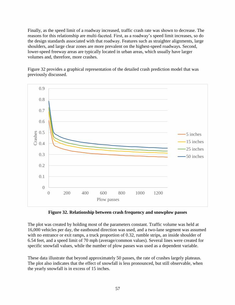
57

Finally, as the speed limit of a roadway increased, traffic crash rate was shown to decrease. The

reasons for this relationship are multi-faceted. First, as a roadway’s speed limit increases, so do

the design standards associated with that roadway. Features such as straighter alignments, large

shoulders, and large clear zones are more prevalent on the highest-speed roadways. Second,

lower-speed freeway areas are typically located in urban areas, which usually have larger

volumes and, therefore, more crashes.

Figure 32 provides a graphical representation of the detailed crash prediction model that was

previously discussed.

Figure 32. Relationship between crash frequency and snowplow passes

The plot was created by holding most of the parameters constant. Traffic volume was held at

16,000 vehicles per day, the eastbound direction was used, and a two-lane segment was assumed

with no entrance or exit ramps, a truck proportion of 0.32, rumble strips, an inside shoulder of

6.54 feet, and a speed limit of 70 mph (average/common values). Several lines were created for

specific snowfall values, while the number of plow passes was used as a dependent variable.

These data illustrate that beyond approximately 50 passes, the rate of crashes largely plateaus.

The plot also indicates that the effect of snowfall is less pronounced, but still observable, when

the yearly snowfall is in excess of 15 inches.

0

0.1

0.2

0.3

0.4

0.5

0.6

0.7

0.8

0.9

0 200 400 600 800 1000 1200

Cra

shes

Plow passes

5 inches

15 inches

25 inches

50 inches

58

Figure 33 presents the safety performance function (SPF) again, only this time the ratio of snow

to plow passes is plotted on the x-axis. This plot illustrates that, in general, the effectiveness of

snowplows plateaus after approximately one pass per half inch of snow. However, this does not

take into consideration the unique conditions of each winter weather event.

Figure 33. Relationship of crash frequency and snow/snowplow pass ratio (in./pass)

Roadway Images

The objective of this section is to investigate potential use of snowplow images to assess

roadway surface, weather, and traffic conditions at/near the time and location of winter weather-

related crashes. However, other potential similar resources (fixed-position cameras) will be

introduced and discussed first.

Fixed-Position Cameras

A network of fixed-position cameras and traffic sensors exists throughout the state, primarily on

Interstates and urban/suburban high-traffic arterials (see Figure 34), which allows Iowa DOT

maintenance staff, the Iowa DOT traffic management center, and the media, as well as the

general public, to continuously monitor conditions.

0

0.1

0.2

0.3

0.4

0.5

0.6

0 0.5 1 1.5 2 2.5 3

Cra

shes

Snow per plow pass

59

Iowa DOT (2017f)

Figure 34. Iowa DOT camera locations

Data are captured continuously or at regular intervals. Through monitoring, changes in roadway,

weather, and traffic conditions can be detected and observed. Post-event assessment may be

conducted by spatially integrating weather-related crashes with the known locations of such

infrastructure, and the image archives temporally mined with respect to reported crash times.

Figure 35 and Figure 36 present example RWIS images spatially and temporally proximate to

several winter weather-related crashes that occurred during the morning of February 12, 2014.

60

Iowa DOT (Iowa Environmental Mesonet 2017a)

Figure 35. Example RWIS image – poor visibility

61

Iowa DOT (Iowa Environmental Mesonet 2017b)

Figure 36. Example RWIS image – traffic congestion

Multiple westbound crashes were reported west of the Interstate 80 RWIS site near the city of

Colfax. Figure 35 conveys the poor visibility conditions at 9:01 a.m., prior to two 9:13 a.m.

crashes located 0.8 and 1.7 miles west of the RWIS site. Figure 36 provides a good contrast in

visibility conditions nearly 30 minutes later, at 9:32 a.m.

Figure 36 also coincides with another crash, located approximately 1.4 miles west of the RWIS

site, reported at 9:30 a.m. Contributing circumstances of this crash included a “previous

accident,” likely one of the 9:13 a.m. crashes, and “road surface conditions.” Westbound traffic

congestion greater than one mile from the reported crash site is clearly visible in Figure 36.

The 9:30 a.m. crash involved a single vehicle and had a derived major cause of

“swerving/evasive action,” which may suggest that the driver was not prepared for the traffic

congestion resulting from the weather/surface conditions and previous crash. All three of the

aforementioned crashes experienced a relatively recent “before” snowplow pass—estimated at 8,

10, and 26 minutes, respectively—and had consistent total snowplow pass frequencies. Slight

differences were observed in the before and after pass frequencies, which may be related to

possible inaccuracies in reported crash time(s).

62

While fixed-position cameras can provide insight into conditions surrounding spatially proximate

winter weather-related crashes, actual crashes may not be within visible range of the RWIS

cameras, such as in Figure 35 and Figure 36. Assumptions are necessary regarding whether the

RWIS-based conditions are generally representative of those at the crash sites. Because of the

limited extent of fixed-position camera and sensor infrastructure off the Interstate system and

major urban/suburban arterials, the set of possible crashes available for analysis is limited to

these known locations. Crash-based, temporal constraints are also present, but given data

collection practices, there is a higher probability that potentially pertinent images exist.

Snowplow Cameras

Unlike fixed-position cameras, snowplow-based images exist throughout the primary highway

system in Iowa, providing a broader view of the system as a whole and expanding possible set of

crashes available for analysis. Because of the mobile nature of snowplows, continuous data are

not available at fixed locations, as locations are constantly changing. Like fixed-position

cameras, location-based constraints impact possible crashes available for analysis, but these

constraints are spatially dynamic in nature, coupled with the crash-based temporal constraints.

As was discussed in “Data Collection, Processing, and Integration,” 19,421 snowplow images,

not limited to the Interstate 80 corridor, were obtained for January 1, 2014 through April 15,

2014. The spatial distribution of these images was presented in Figure 5. A one-mile spatial

proximity was utilized to integrate these snowplow images with crashes occurring during the

same period. A total of 3,987 winter crashes were located within one-mile of the snowplow

images (see Figure 37).

63

Figure 37. Snowplow images and crashes within one mile

Using ESRI ArcMap “Generate Near Table” tool, a database table was created presenting the

relationship between each winter crash and all snowplow images located within the user-defined

search radius. A one-mile search radius was employed, assuming surface/weather conditions

were relatively similar within this proximity. Expanding the search radius may increase the

number of snowplow images on adjacent or intersecting roadways, requiring more manual

inspection later. Conditions may also become less representative as the distance increases, even

along the same roadway. That said, narrowing the search radius could potentially limit crashes of

interest.

A total of 86,364 records were returned in the resulting “near table.” Each record represents a

unique crash-snowplow image combination, the corresponding distance between the crash and

image, and a proximity-based ranking for each crash. A one-to-many relationship may exist

between both crashes and images. In other words, a given crash may be associated with multiple

snowplow images, and a given snowplow image may be associated with multiple crashes.

By integrating the underlying crash and snowplow image attributes with the “near table” results,

all images captured within 60 minutes before or after a crash were identified using the

corresponding date/time attributes. One hundred seventy-nine records satisfied the criteria of

being within one mile and one hour of a winter crash, representing 103 unique crashes and 174

unique snowplow images. Figure 38 presents the locations of these crashes and images, many of

which appear in the general vicinity of fixed-position camera sites (see Figure 34).

64

Figure 38. Snowplow images and crashes within one mile and one hour

Through use of the crash and snowplow image date/time attributes as well as the “near table”

distance attribute, records were reviewed based on spatial proximity and time difference between

winter crash and snowplow image. Primary factors reviewed, through visual inspection and

attribute comparisons, included the following:

Time of day. Surface, weather, and traffic conditions were difficult to assess in snowplow

images taken at nighttime or dark conditions.

Direction of travel. On divided roadways, crashes and the corresponding snowplow images

could potentially be in different directions of travel.

Roadway of interest. Crashes and snowplow images on different roadways, such as parallel

routes or near intersections, could potentially be associated with each other in the “near

table.”

No actual crash events were observed among the snowplow images reviewed; however, several

images were taken at approximately the same time and/or location as a crash. For example, over

20 images were within approximately one-tenth of a mile of the reported crash location. Figure

39 shows a snowplow image taken at the same time, intersection, and direction of travel

(eastbound) as a winter weather-related crash.

65

Iowa DOT

Figure 39. Snowplow image, Example 1

Precipitation is not immediately apparent, but the pavement surface is snowy and slushy. While

reported crash time and location inaccuracies may exist, the image likely provides a fairly

accurate representation of the surface conditions at the time of the crash.

Figure 40 presents the spatial relationship between a snowplow image (with plow direction of

travel presented as an arrow) and winter weather-related crash location on eastbound Interstate

80.

66

Figure 40. Snowplow image versus crash location, Example 2

Figure 41 presents the snowplow image itself.

Iowa DOT

Figure 41. Snowplow image, Example 2

Both atmospheric snow and snow on the pavement are visible. Snow patterns on the roadway

may suggest windy conditions. The image was taken 11 minutes after the crash, approximately

1,800 feet upstream (in advance of the crash location) in the eastbound direction. Multiple

67

snowplow passes were observed within the 2 hours before and after the crash, with the most

recent passes estimated at 19 minutes before and 3 minutes after the crash. Crew reports

indicated Phase 1 operations occurring during two periods of the day. Snow and blowing snow

were also reported.

Figure 42 presents the spatial relationship between a snowplow image and winter weather-related

crash location on westbound Interstate 80.

Figure 42. Snowplow image versus crash location, Example 3

Figure 43 shows the snowplow image itself, taken from the right shoulder.

68

Iowa DOT

Figure 43. Snowplow image, Example 3

Unfortunately, windshield icing limits a clear view of conditions, although snow can be seen

sticking to the pavement. The image was taken 3 minutes after the crash, approximately 500 feet

downstream (beyond the crash location) in the westbound direction. Multiple snowplow passes

were observed within the 2 hours before and after the crash, with the most recent passes

estimated at 16 minutes before and 10 minutes after the crash. Crew reports indicated Phase 1

operations throughout the day. Snow was reported during most of the day, and blowing snow

was reported during half of the day.

Figure 44 presents the spatial relationship between a snowplow image and non-weather-related

crash location on westbound Interstate 80 during the morning weekday traffic peak. As was

noted previously, this analysis was not limited to weather-related crashes.

69

Figure 44. Snowplow image versus crash location, Example 4

Figure 45 presents the snowplow image itself.

Iowa DOT

Figure 45. Snowplow image, Example 4

Surface conditions appear wet or normal. Traffic is visible, possibly due to the morning commute

and/or crash. The image was taken 22 minutes after the crash, approximately 240 feet upstream

(in advance of the crash location) in the westbound direction. Multiple snowplow passes were

70

observed within the 2 hours before and after the crash, with the most recent passes estimated at

the same time as the crash and 28 minutes after the crash. Crew reports indicated Phase 1

operations throughout the morning hours, including at the time of the crash. Snow was reported

from approximately midnight to 1:00 a.m., and blowing snow was reported as ending within 2

hours of the time of the crash. Unlike the previous example snowplow images, the conditions

visible in the image do not necessarily immediately convey surface or weather conditions under

which crashes may be more probable. In fact, the crash was not reported as weather related, even

though it occurred during Phase 1 operations. It is possible that coding inaccuracies existed in the

crash report, or that the crash itself had nothing to do with winter weather. Regardless,

integrating other supporting information, such as maintenance crew reports, precipitation reports,

and snowplow AVL data, provided greater insight into underlying or tertiary conditions.

Figure 46 presents INRIX-based average traffic speeds for the one hour before and after the

previous three example crashes.

Figure 46. Example crash average traffic speeds

The average traffic speeds for the TMCs corresponding to the example crash locations possessed

high confidence indicators during the two hours of interest. In Figure 46, time 0 represents the

reported time of the crash. While temporal latency may exist in the real-time speed data,

inaccuracies may exist in the reported crash times. Figure 46 shows reductions in average speeds

after each crash. However, the time, degree, and duration of these reductions vary. Interestingly,

the most significant, immediate and sustained speed impact is apparent in Example 4, which is

the non-weather-related crash. For the weather-related crashes (Examples 2 and 3), short

duration speed reductions appear to occur prior to the crashes, followed by an increase in average

speeds for a short duration. Speeds decrease again, more noticeably, within approximately 10 to

30 minutes after the reported crash time. Speeds then begin to increase to near pre-crash

averages. A second, more significant reduction in average speeds occurs for Example 3, which

may be related to another crash, traffic congestion, or poor conditions. In general, Figure 46

30

35

40

45

50

55

60

65

70

-60-55-50-45-40-35-30-25-20-15-10 -5 0 5 10 15 20 25 30 35 40 45 50 55

Ave

rage

Sp

eed

(m

ph

)

Time (minutes)

Ex. 2 Ex. 3 Ex. 4

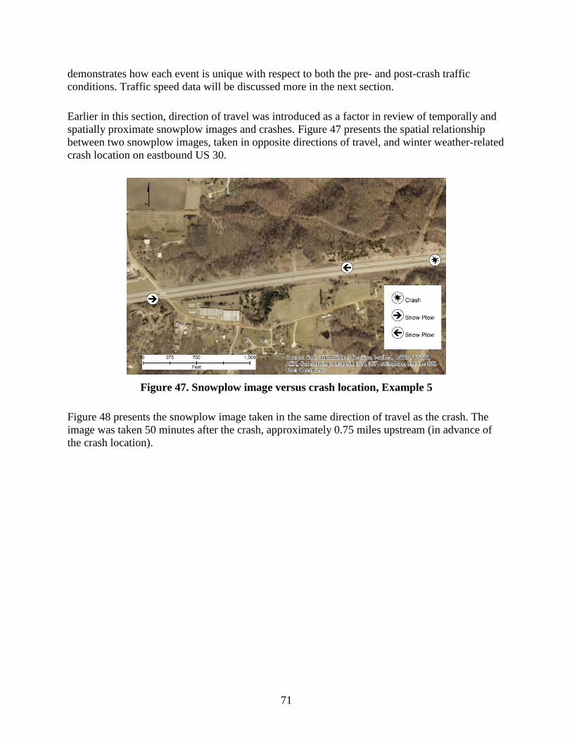
71

demonstrates how each event is unique with respect to both the pre- and post-crash traffic

conditions. Traffic speed data will be discussed more in the next section.

Earlier in this section, direction of travel was introduced as a factor in review of temporally and

spatially proximate snowplow images and crashes. Figure 47 presents the spatial relationship

between two snowplow images, taken in opposite directions of travel, and winter weather-related

crash location on eastbound US 30.

Figure 47. Snowplow image versus crash location, Example 5

Figure 48 presents the snowplow image taken in the same direction of travel as the crash. The

image was taken 50 minutes after the crash, approximately 0.75 miles upstream (in advance of

the crash location).

72

Iowa DOT

Figure 48. Snowplow image, Example 5 (eastbound)

Figure 49 presents the snowplow image taken in the opposite direction of travel of the crash.

Iowa DOT

Figure 49. Snowplow image, Example 5 (westbound)

The image was taken 20 minutes before the crash, approximately 0.25 miles downstream

(beyond the crash location). Both of these images generally depict consistent surface and weather

conditions in both directions of travel for greater than one hour. The conditions were likely

representative of those at the time of the crash as well as showing the maintenance challenges of

Phase 1 operations.

73

Both fixed-position cameras and snowplow-based images can provide insight into surface,

weather, and traffic conditions surrounding a crash experience. Crash and image datasets may be

systematically integrated spatially and temporally to facilitate after-event assessment. Additional

images may also be identified to investigate location-based conditions prior to or following a

crash or simply when no crash occurred. As noted previously, integrating supporting

information, such as maintenance crew reports, precipitation reports, snowplow AVL data, and

RWIS roadway and weather data may provide greater understanding of conditions as a whole.

Such understanding may be beneficial in assessing whether operational expectations were

satisfied, and if modifications may be considered. While the emphasis of this section was on

weather-related crashes, it is important to note that mobile and fixed-position camera images

may also be used to track precipitation, visibility, roadway surface conditions, and traffic along a

storm track both during the event and for an after-event assessment.

Traffic Speed

As with cameras, a network of fixed-position traffic sensors exists throughout Iowa. The Iowa

DOT also maintains a smaller set of portable traffic sensors, which are often deployed at or near

work zones and other locations of temporary interest. While these sensors provide detailed site-

specific traffic speed and volume data by lane, the coverage is still somewhat limited. INRIX

traffic speed data, collected through probe vehicles, is more comprehensive in nature, providing

directional, segment-level, average traffic speeds throughout the system. Data are most complete

and accurate on higher-volume roadways, such as Interstates, expanding the possible set of

crashes available for analysis to the entire Interstate 80 corridor. Therefore, the emphasis of this

study is on INRIX traffic speed data.

In the previous section, use of INRIX data was introduced to show average traffic speeds relative

to three reported crashes. Even for this limited set of crashes, the individual nature of traffic

conditions for each event was apparent. To more broadly investigate general traffic speed

tendencies and trends with respect to winter crash experience, speeds within 60 minutes of all

winter crashes during the 2013 and 2014 calendar winters along the Interstate 80 corridor were

analyzed. Pre- and post-crash speed conditions will be presented, and non-weather-related and

weather-related crashes compared. The primary objective of this investigation was to provide a

high level, descriptive introduction to traffic speed data for possible later use in prediction of

crash conditions as well as to demonstrate the impacts of crashes on mobility. Such application

would require more rigorous statistical analysis.

Appropriate traffic speed records were selected based on the directional TMC assigned to each

crash and timestamp within 60 minutes of the reported time of the crash. When appropriate,

traffic speed records were associated with multiple crashes, depending on the TMC and time of

the other crashes. Table 6, from earlier in the report, presents the total number of records

identified by year and direction of travel: approximately 119,000 in 2013 and 132,000 in 2014.

Once identified, all records were normalized to the reported time of the crash. Time 0

represented the time of the crash, negative time values represented minutes before the crash, and

positive time values represented elapsed minutes after the crash. All speed records were utilized,

regardless of the reported confidence. The confidence of real-time speeds was typically high for

74

Interstate 80 but could decrease during periods of low traffic volumes. Ninety-eight percent of

the traffic speed records were reported as real-time data, and the confidence indicator for all

records was 89 of 100.

Crashes were grouped by calendar year, crash report-based winter weather conditions (weather-

related and non-weather-related), and posted speed limit of the roadway of occurrence. The

following eight distinct groups, and corresponding number of crashes, resulted:

2013 non-winter weather-related crashes, posted speed limit less than 70 mph (169 crashes)

2013 winter weather-related crashes, posted speed less than 70 mph (235 crashes)

2013 non-winter weather-related crashes, posted speed limit of 70 mph (230 crashes)

2013 winter weather-related crashes, posted speed limit of 70 mph (384 crashes)

2014 non-winter weather-related crashes, posted speed limit less than 70 mph (228 crashes)

2014 winter weather-related crashes, posted speed less than 70 mph (230 crashes)

2014 non-winter weather-related crashes, posted speed limit of 70 mph (315 crashes)

2014 winter weather-related crashes, posted speed limit of 70 mph (360 crashes)

To simplify presentation of the data, the average and standard deviation of traffic speed for one-

minute intervals were calculated for each distinct group. By doing so, the TMC average speed

must be assumed uniform and representative for each crash location. Additionally, given the

number of crashes in each group—ranging from 169 to 360—the sensitivity of each resulting

average speed to extreme values, or lower confidence, may be assumed to be low. Possible

limitations for consideration in interpretation of results include the following:

The one-minute speed intervals represent average values for all lanes of travel for the TMC

as a whole.

Historic or a combination of historic and real-time speed data may be represented. Based on

the previously noted confidence, the overall frequency of occurrence was low.

Average speed data may occasionally not exist for a one-minute interval.

Temporal latency may exist in the average traffic speed records.

Inaccuracies may exist in reported crash times.

Given average TMC length, often between interchanges, localized speed variations may

occur. Possible impacts may be limited in future analyses using INRIX data, as XD segments

are shorter, and average traffic speeds are also provided at frequent intervals.

Average traffic speeds represent all lanes of travel, unlike other Iowa DOT traffic sensor data

which can provide lane specific details.

Average traffic speeds do not convey differences in speeds among vehicles.

Traffic volumes are unknown, unlike other Iowa DOT traffic sensor data.

Probe vehicles, such as fleet and commercial vehicles, may travel at lower speeds than the

traffic mix as a whole.

The maximum reported average traffic speed was 75 mph.

Figure 50 presents information on average TMC traffic speeds for 60 minutes before and after

each winter weather-related crash (2013 and 2014 calendar winters) on Interstate 80.

75

a. AVG traffic speeds, non-70 mph limit (2013)

b. AVG traffic speeds, 70 mph limit (2013)

c. AVG traffic speeds, non-70 mph limit (2014)

d. AVG traffic speeds, 70 mph limit (2014)

e. STD traffic speed, non-70 mph limit

f. STD traffic speed, 70 mph limit

g. AVG traffic speed comparison, non-70 mph

limit

h. AVG traffic speed comparison, 70 mph limit

Figure 50. Traffic speed overview

76

The right column presents information for TMC sections with a speed limit less than 70 mph,

while the right column presents the same information for TMC sections with a speed limit of 70

mph. In Figure 50 a, b, c, and d, the wide range of traffic speeds at which weather-related crashes

occurred is clearly conveyed. Crashes occurred at speeds ranging from less than 10 mph to more

than 70 mph. Data points are dispersed throughout each figure, with a greater dispersion post-

crash. Crashes occurring at high speeds may represent motorists overdriving surface and weather

conditions. Crashes at lower speeds may indicate motorists adjusting their driving behavior to

conditions and/or the presence of congestion, due to conditions or previous crashes.

Figure 50 e and f use standard deviation (SD) to convey the variation of speeds at which crashes

occur. Both winter weather-related and non-weather crashes are compared. In general, SD

among weather events increases from one hour before the crash (approximately 8 to 10 mph)

until approximately 30 minute or more after the crash. This continuous increase may suggest that

traffic is less impacted by conditions as the time before the crash increases, possibly before

conditions have deteriorated. The higher, post-crash speed variations can be expected due to

crash-related traffic disruptions, unique event characteristics, and conditions.

Prior to a crash, the SD for winter weather-related crashes was consistently higher than for non-

weather-related crashes, indicating that driving behavior may be more inconsistent among winter

weather events. Speed variations continue to be higher throughout the analysis period for

sections with a speed limit of 70 mph. The TMCs associated with these are longer, possibly

limiting the ability to capture localized speed changes. The traffic volumes are also lower,

allowing more freedom in speed selection.

Figure 50 g and h present the combined average speeds for weather and non-weather-related

crashes. These figures, as well as the six order polyline regression lines in Figure 50 a and b

convey that the average pre-crash and crash speeds for weather-related crashes are 55 mph and

greater, which is in the higher range of speeds observed. However, crash speeds are

approximately 10 mph (or more) below the posted speed limit.

Prior to a crash, the average speeds for winter weather-related crashes were approximately 5 mph

lower than non-weather-related crashes. A possible explanation is motorists changing driving

behavior due to conditions. Average pre-crash speeds appear relatively stable, if not slightly

decreasing, for weather and non-weather crashes on less than 70 mph sections and non-weather

crashes on 70 mph sections. A more noticeable consistent decline is visible for weather-related

crashes on 70 mph sections.

Among all years and crash types, post-crash speeds appear less impacted on 70 mph sections

with a non-weather crash. As mentioned previously, this may be due to lower traffic volumes in

rural areas. Non-weather-related crashes may also be more isolated in nature, with fewer

underlying contributing circumstances to impact traffic. More dramatic changes in post-crash

speeds are observed on sections with a speed limit less than 70 mph. These roads typically are

urban/suburban and have higher traffic volumes; therefore, the impact of crashes can be more

pronounced. This is also apparent in non-weather crashes. For all crashes, average traffic speeds

did not return to crash or pre-crash levels for at least an hour after the crash. Recovery was

77

slower for weather-related crashes, demonstrating the general mobility-related impacts of these

crashes coupled with conditions.

Because of the wide variation of average traffic speeds observed in Figure 50, the difference in

average traffic speed between the reported time of the crash (time 0) and 60 minutes before and

after the crash were calculated. In other words, the speed along the TMC at the time of the crash

was compared to the speed along the TMC before and after the crash. This was done to

normalize the data and investigate whether changes in pre-crash relative speed, instead of actual

speed, may possibly indicate deteriorating conditions. Figure 51 presents this information on

relative TMC traffic speeds for 60 minutes before and after each winter weather-related crashes

(2013 and 2014 calendar winters) on Interstate 80.

78

a. AVG traffic speeds, non-70 mph limit (2013)

b. AVG traffic speeds, 70 mph limit (2013)

c. AVG traffic speeds, non-70 mph limit (2014)

d. AVG traffic speeds, 70 mph limit (2014)

e. STD traffic speed, non-70 mph limit

f. STD traffic speed, 70 mph limit

g. AVG traffic speed comparison, non-70 mph

limit

h. AVG traffic speed comparison, 70 mph limit

Figure 51. Relative traffic speed overview

79

The right column presents information for TMC sections with a speed limit less than 70 mph,

while the right column presents the same information for TMC sections with a speed limit of 70

mph.

Figure 51 a, b, c, and d clearly convey the wide range of relative traffic speeds. The speed at the

time of the crash could be nearly 50 mph more than the pre-crash speed to over 60 mph less than

the pre-crash speed. As expected, the pre-crash relative speeds were generally higher and greater

than 0 mph, meaning that the pre-crash average speeds were greater than those at the time of the

crash. More variation in relative speed was observed post-crash. As discussed previously, this is

likely due to crash-related traffic disruptions, unique event characteristics, and conditions.

Figure 51 e and f use SD to convey the variation of relative speeds. Both winter weather-related

and non-weather crashes are compared. The standard deviation among weather events decreases

from one hour before the crash (greater than 10 mph) until the time of the crash. Relative speeds

are converging among events, possibly reflecting motorists reacting to conditions. The rapidly

changing SD immediately proximate to the reported crash time (both before and after) may be

due, in part, to inaccuracies in crash time reporting and latency of speed data.

In general, the trends observed for the SD of relative speeds are consistent with actual speeds.

Prior to a crash, the standard deviation for winter weather-related crashes was consistently higher

than non-weather-related crashes. For sections with a 70 mph speed limit, relative speed

variations were higher throughout the analysis period. As expected, the largest relative speed

variations were observed post-crash.

Figure 51 g and h present the combined average relative speeds for weather and non-weather-

related crashes. Pre-crash relative speeds are only a few miles per hour greater than crash speeds.

However, compared to actual speeds, fewer differences are observed between weather and non-

weather crashes. Average pre-crash relative speeds appear relatively stable until close to the time

of the crash. A more noticeable consistent decline is visible for weather-related crashes on 70

mph sections.

Among all years and crash types, post-crash relative speeds were nearest to zero on 70 mph

sections with a non-weather crash. As mentioned previously, non-weather-related crashes along

such rural roads may be more isolated in nature, with fewer underlying contributing

circumstances to impact traffic. The greatest relative speeds (less than the speeds at the time of

the crash) were post-crash on sections with a speed limit less than 70 mph. Weather crash-related

relative speeds were also higher than non-weather crashes on 70 mph sections. For all crashes,

the relative speeds remained less than 0 mph for at least an hour following the crash.

While normalizing the speed data facilitated comparison of speed among events, it could not take

into consideration the unique weather conditions, including spatial and temporal components,

surrounding each event. Large variations in speed were observed. Unfortunately, it does not

appear that the general pre-crash speed patterns presented in Figure 50 and Figure 51 may be

utilized for crash prediction. This is not necessarily unexpected given the variety of road sections

and weather events being represented. However, opportunities may exist to utilize localized

80

speed monitoring, coupled with weather data, to identify unstable and changing conditions, with

subsequent messaging informing motorists of conditions. Traffic speeds may then be reduced

and harmonized, improving both safety and mobility.

81

CONCLUSIONS AND RECOMMENDATIONS

Historically, the relationships among winter weather maintenance practices, safety, and mobility

have been difficult to systematically assess and quantify. Through acquisition of snowplow AVL

and image data as well as system-wide traffic data, more comprehensive analyses and

assessments are feasible, facilitating more refined and broader location-specific analyses. The

Iowa DOT may use these data resources to supplement existing efforts to monitor traffic,

weather, and surface conditions and direct their corresponding actions and reactions.

The primary emphasis of this project was to demonstrate integration of historic crash data with

maintenance and traffic data in an attempt to gain a better understanding of the conditions during

which these crashes occur. A limitation of the approach was that the unique nature of and

circumstances surrounding each event could not be considered and addressed. An additional

challenge was the appropriate, effective, and practical use of the underlying datasets given their

sheer magnitude. For example, nearly 2 million AVL records existed for the Interstate 80

corridor alone during the winter months of a single calendar year. Nearly 20,000 snowplow

images existed for a limited portion of the state during a two-month period. Both of these

datasets will only continue to expand with continued implementation and installation. Traffic

speed data will continue to grow as they become more spatially and temporally discrete.

Along the Interstate 80 corridor, winter weather-related crashes were proportionally higher

during the morning hours, which may be influenced by several factors. Crash experience during

this time, when people are typically departing for work and school, highlights the need for

advanced, appropriate, consistent, coordinated, and accurate motorist-directed messaging from

the Iowa DOT and its partners.

The majority of days during which Phase 1 maintenance operations occurred experienced no

weather-related crashes. There were also a limited number of days during which a weather-

related crash occurred, and no Phase 1 operations were reported. Therefore, from a safety

perspective, Phase 1 maintenance operations appear broadly successful and to have occurred

during appropriate times. An opportunity may exist to review the days during which weather-

related crashes have occurred and determine pertinent characteristics. For example, a limited

number of weather events may contribute more heavily to crash experience.

With respect to snowplow AVL data, more crashes occurred as the time interval increased

between the last snowplow pass and time of the crash. The period of time with the single highest

percentage of crashes was 90 minutes to 2 hours before the crash and within 30 minutes after the

crash. This may represent an approximate 2-hour snowplow return time, or the presence of traffic

conditions impeding snowplow progress. In general, fewer passes occurred prior to the crash.

The average snowplow pass frequency was higher following the crash, with the highest pass

frequencies occurring immediately following the reported time of the crash. More crashes had no

observed snowplow passes 2 hours before the crash compared to 2 hours after the crash, 24

percent and 10 percent, respectively. This may be the result of missing or incomplete AVL data,

or it could indicate that crashes are occurring early in weather events, possibly prior to Phase 1

operations.

82

Further investigation of the crash time interval and absence of “before” AVL data may be

warranted for additional routes and years. If these previous findings are verified, alternative

maintenance operations protocols could potentially be explored.

The majority of winter weather-related crashes experienced multiple snowplow passes within 2

hours before and after the crash. This may indicate that crashes are occurring early in the weather

event, during periods of high snowplow activity, and/or along multilane sections. In the future,

the differences and similarities between the low and high pass crashes could be further explored

as case studies.

As snowplow frequency increases for a specific amount of snow, the rate of traffic crashes per

million vehicle miles travelled decreases. This demonstrates, in part, the safety-related

effectiveness of winter maintenance. However, from a weather perspective, the corresponding

statistical model only considered snowfall. Additionally, the AVL-related analyses did not take

into consideration other factors, such as traffic speed, congestion, and weather event type,

intensity, and duration, which may impact snowplow operations. Development of an expanded

statistical model, including additional weather-related and other parameters, may be warranted.

Micro-level case studies may also be beneficial in quantifying the impacts of extraneous factors.

Other potentially important considerations for maintenance operations include the positive

correlation between traffic volume and crash frequency, elevated crash frequency on westbound

Interstate 80, elevated crash risk where entrance and exit ramps are present, and the inverse

relationship between speed limit and crash rate. Many, if not all, of the above may already be

addressed in operations.

Both fixed-position cameras and snowplow-based images can provide insight into surface,

weather, and traffic conditions surrounding a crash experience. Spatial and temporal integration

of crash and image datasets may facilitate after-action assessment and investigation of location-

based conditions prior to and following a crash. As most crashes result from driver error, these

conditions may also be compared to locations where no crash has occurred to provide

perspective. Better understanding of crash conditions may be beneficial in assessing whether

operational expectations were satisfied, and if modifications could be considered.

Unfortunately, because of the large variation of both speed and relative speeds among crash

events, pre-crash speed patterns could not be utilized for crash prediction. This is not entirely

unexpected given the variety of road sections and weather events being analyzed. However,

mobility-related impacts were clearly identifiable by lower pre- and post-crash speeds. The post-

crash impacts were greatest, with speeds not returning to pre-crash levels within the 60 minute

analysis period. That said, opportunities may exist to utilize localized speed monitoring, coupled

with weather data, to identify unstable and changing conditions, with subsequent messaging

informing motorists of traffic conditions. This may limit dangerous speed differentials.

As a whole, this project has promoted use of extensive rich datasets to investigate weather-

related impacts on mobility and safety and evaluate possible opportunities for winter

maintenance operations. New capabilities were introduced; existing capabilities expanded; and

83

limitations, challenges, and potential areas for additional investigation identified. Ideally,

through use of this work, the negative highway-related impacts of winter weather may be

reduced.

85

REFERENCES

Barajas, V.L., Z. Wang, M. Kaiser, and Z. Zhu. 2017. Improving Estimates of Real-Time Traffic

Speeds during Weather Events for Winter Maintenance Performance Measurement.

Midwest Transportation Center, Institute for Transportation, Iowa State University,

Ames, IA.

Barreto, H. and F. M. Howland. 2008. The P Value Calculator Excel Add-in Software for

Introductory Econometrics, Version: 29. Introductory Economics. Cambridge University

Press, Cambridge, U.K.

http://www3.wabash.edu/econometrics/EconometricsBook/Basic%20Tools/ExcelAddIns/

PValueCalculator.htm.

Black, A.W. and T.L. Mote. 2015. Effects of Winter Precipitation on Automobile Collisions,

Injuries, and Fatalities in the United States. Journal of Transport Geography, Vol. 48, pp.

165–175.

El-Basyouny, K., S. Barua, and M. T. Islam. 2014. Investigation of Time and Weather Effects on

Crash Types using Full Bayesian Multivariate Poisson Lognormal Models. Accident

Analysis and Prevention, Vol. 73, pp. 91–99.

FHWA. 2017. Road Weather Management Program, Snow and Ice. Federal Highway

Administration, Washington, DC.

https://ops.fhwa.dot.gov/weather/weather_events/snow_ice.htm.

INRIX. 2014. Case Studies: Iowa DOT. INRIX, Kirkland, WA. http://inrix.com/case-

studies/iowa-dot/.

Iowa Environmental Mesonet. 2017a. Archived Iowa RWIS Webcam Imagery. Iowa DOT,

Ames, IA. https://mesonet.agron.iastate.edu/RWIS/camera.phtml#IDOT-053-

02_201402121501.jpg.

Iowa Environmental Mesonet. 2017b. Archived Iowa RWIS Webcam Imagery. Iowa DOT,

Ames, IA. https://mesonet.agron.iastate.edu/RWIS/camera.phtml#IDOT-053-

02_201402121532.jpg.

Iowa DOT. 2017a. Performance, Winter Operations. (Weather, Cost, Outcomes) Iowa

Department of Transportation, Ames, IA. https://iowadot.gov/performance/winter-

operations#22607388-historic.

Iowa DOT. 2017b. Maps, Vehicle-Miles Traveled (VMT). Iowa Department of Transportation,

Ames, IA. https://iowadot.gov/maps/data/vehicle-miles-traveled.

Iowa DOT. 2017c. Systems Operations Bureau. Iowa Department of Transportation, Ames, IA.

https://iowadot.gov/systemsoperations/home.

Iowa DOT. 2017d. Track a plow. Iowa Department of Transportation, Ames, IA.

http://iowadot.maps.arcgis.com/apps/webappviewer/index.html?id=3d5bc4ec8c474870a1

9c7e8f44b39c9c.

Iowa DOT. 2017e. Performance, Winter Operations, Weather Events. Iowa Department of

Transportation, Ames, IA. https://iowadot.gov/performance/winter-

operations#22606381-events.

Iowa DOT. 2017f. 511 Iowa, Cameras and Speeds. Iowa Department of Transportation, Ames,

IA.

https://hb.511ia.org/#camerasHome?layers=cameras%2CgoogleTraffic&timeFrame=TO

DAY

86

Koeberlein, R., D. Jensen, and M. Forcier. 2015. Relationship of Winter Road Weather

Monitoring to Winter Driving Crash Statistics. Paper presented at the Transportation

Research Board 94th Annual Meeting, January 11–15, Washington DC.

Krechmer, D., N. Perry, L. Destro, and S. Gallaher. 2012. Weather Delay Costs to Trucking.

Federal Highway Administration, Washington, DC.

https://rosap.ntl.bts.gov/view/dot/3384.

Kuemmel, D.A., and R.M. Hanbali. 1992. Accident Analysis of Ice Control Operations. The Salt

Institute, Alexandria, VA. http://www.trc.marquette.edu/publications/IceControl/ice-

control-1992.pdf.

Lane, D. M. 2009. Tests of Differences between Proportions. Rice University, Houston, TX.

http://davidmlane.com/hyperstat/B73479.html.

McNamara, M., R. Sakhare, H. Li, M. Baldwin, and D. Bullock. 2017. Integrating Crowdsource

Probe Vehicle Traffic Speeds into Winter Operations Performance Measures. Paper

presented at Transportation Research Board 96th Annual Meeting, January 8–12,

Washington DC.

Menard, T., J. Lund, J. Miller, and T. Petersen. 2012. 907-Plow–Anchorage’s Approach to Real-

Time Snowplow Tracking. Paper presented at the 15th International IEEE Conference on

Intelligent Transportation Systems, September 16–19, Anchorage, AK.

Moore, D., G. McCabe, W. M. Duckworth, and S. L. Sclove. 2003. The Practice of Business

Statistics, First Edition. W. H. Freeman, London, UK.

Murphy, R., R. Swick, and G. Guevara. 2012. Best Practices for Road Weather Management,

Version 3.0. Project Report No. FHWA-HOP-12-046, Federal Highway Administration,

Washington DC.

https://ops.fhwa.dot.gov/publications/fhwahop12046/fhwahop12046.pdf.

Norrman, J., M. Eriksson, and S. Lindqvist. 2000. Relationships between Road Slipperiness,

Traffic Accident Risk, and Winter Road Maintenance Activity. Climate Research, Vol.

15, No. 3, pp. 185–193.

Shaheed, M.S., K. Gkritza, A.L. Carriquiry, and S. L. Hallmark. 2016. Analysis of Occupant

Injury Severity in Winter Weather Crashes: A Fully Bayesian Multivariate Approach.

Analytic Methods in Accident Research, Vol. 11, pp. 33–47.

Usman, T., L. Fu, and L.F. Miranda-Moreno. 2011. Winter Road Safety: Effects of Weather,

Maintenance Operations and Road Characteristics. Paper presented at First International

Conference on Transportation Information and Safety, June 30–July 2, Wuhan, China.

Usman, T., L. Fu, and M. S. Perchanok. 2012. Application of Collision Prediction Models for

Quantifying the Safety Benefit of Winter Road Maintenance. Transportation Research

Circular E-C162: Winter Maintenance and Surface Transportation Weather, pp. 29-42.

http://onlinepubs.trb.org/onlinepubs/circulars/ec162.pdf.

Ye, Z., D. Veneziano, and X. Shi. 2013. Estimating Statewide Benefits of Winter Maintenance

Operations. Transportation Research Record: Journal of the Transportation Research

Board, No. 2329, pp. 17–23.

Visit www.InTrans.iastate.edu for color pdfs of this and other research reports.

THE INSTITUTE FOR TRANSPORTATION IS THE FOCAL POINT FOR TRANSPORTATION AT IOWA STATE UNIVERSITY.

InTrans centers and programs perform transportation research and provide technology transfer services for government agencies and private companies;

InTrans manages its own education program for transportation students and provides K-12 resources; and

InTrans conducts local, regional, and national transportation services and continuing education programs.