Operational availability analysis of generators in steam turbine ...

Vol.:(0123456789)

SN Applied Sciences (2020) 2:779 | https://doi.org/10.1007/s42452-020-2520-y

Research Article

Operational availability analysis of generators in steam turbine power plants

Nivedita Gupta1 · Monika Saini1 · Ashish Kumar1

Received: 19 September 2019 / Accepted: 13 March 2020 / Published online: 30 March 2020 © Springer Nature Switzerland AG 2020

AbstractThe main aim of this study is to explore the availability and profitability of generators, which are key units of steam turbine power plants, considering exponential failure and arbitrary repair time distributions. A Markov birth–death process and supplementary variable technique are used to evaluate system effectiveness measures. Such a generator mainly consists of seven repairable components arranged in a series configuration. A stochastic model of the generator is developed, and the Chapman–Kolmogorov differential difference equation of the system derived. Finally, the results for the steady-state availability and profitability of the system are obtained for a particular case that will be helpful to system designers to enhance the performance of plants to some extent.

Keywords Generator · Steam turbine power plant · Markov birth–death process · Availability · Chapman–Kolmogorov differential difference equations

1 Introduction

As populations exhibit rapid growth, the consumption of elec-tricity by domestic and commercial clients is increasing, with corresponding increasing expectations regarding the energy that power plants can produce. The main aim of any power plant is to maximize its capacity, which is only possible if it can remain operative with high availability. Successful operation of steam turbine power plants depends on successful functioning of its subsystems. In the current age, due to the complexity of such systems and fundamental issues, power plants face many operational challenges and cannot achieve excellent perfor-mance. The performance of any plant depends upon the reli-ability of its components. Through the use of highly reliable subunits/components and perfect maintenance, higher avail-ability can be achieved. Failure is an unavoidable circumstance but can be avoided for some time by implementing reliability improvement techniques. Some of the main causes of power plant failure include poor maintenance, lack of good operators,

inadequate testing, etc., resulting in random system failures and subsequent unavailability. It thus becomes necessary to conduct maintenance of even well-designed components from time to time. Management always wishes to achieve high reliability but with low investment. The main aim of the present study is to determine the most critical component which con-tributes significantly to the operational availability and profit-ability of such systems. A Markov birth–death process and sup-plementary variable technique are used in the system analysis. The data associated with failure and repair rates, expenditure, and revenue are taken arbitrarily based on discussions with maintenance personnel at a plant situated in the central part of India. Sabouhia et al. [1] recommended the consideration of all failure and repair rates as exponentially distributed. There-after, for different combinations of failure and repair rates of subsystems, the availability and profitability of the system are analyzed, and their variation recorded. Such information on the variation of availability can be applied to identify the most sensitive subsystems, based on which proper maintenance

* Monika Saini, [email protected] | 1Department of Mathematics and Statistics, Manipal University Jaipur, Jaipur, Rajasthan 303007, India.

Vol:.(1234567890)

Research Article SN Applied Sciences (2020) 2:779 | https://doi.org/10.1007/s42452-020-2520-y

policies could be planned to improve the performance of the system.

This manuscript is organized into five sections, includ-ing this introductory part. A detailed literature review is presented in Sect. 2. A system description, notation, and state transition diagram are provided in Sect. 3. The sto-chastic analysis is described in Sect. 4, while the numerical analysis and conclusions are given in the final section.

2 Literature review

Cox [2] first coined the term “supplementary variable tech-nique” and obtained reliability measures for a non-Markovian system. Kumar et al. [3] used a Markov birth–death process to depict the steady-state behavior of a desulfurization sys-tem, while Arora and Kumar [4] adopted this methodology for availability analysis of steam and power generation systems. In that work, the failure and repair rates of all subsystems were considered to be exponentially distributed. Furthermore, the derived results could be used to formulate maintenance poli-cies for the system. A detailed introduction to reliability and maintainability theories was presented in Ebeling [5]. Billinton and Allan [6] explained the tools and theories used in reliabil-ity evaluation of engineering systems. Gupta and Tewari [7] and Tewari et al. [8] focused on simulation modeling of ther-mal power plants. In all this published work, all the subsystems were considered to be single complex systems. Carazas et al. [9] developed a stochastic model for heat recovery steam generators to determine the availability of the system. Heat recovery steam generators (HRSGs) are extensively used in thermal power plants. HRSGs installed in combined-cycle power plants have been studied as a case study for reliability analysis. Balagurusamy [10] explained some basic concepts of reliability theory that are useful for system analysis, including quality, probability, Laplace transforms, failure curves, various hazard models, and redundancy. A 210-MW coal-fired ther-mal power plant situated in the eastern region of India was analyzed as a case study by Adhikarya et al. [11]. Reliability, availability, and maintainability (RAM) analysis of the plant was carried out in order to propose the maintenance time of the plant to enhance its availability and performance and ensure a proper power supply. Various other system characteristics such as mean time to failure (MTTF) and the cost–benefit tradeoff for single- and two-unit systems have been exten-sively studied by many researchers such as Singh et al. [12], Kumar et al. [13], Kumari et al. [14], Kumar and Saini [15], and Saini and Kumar [16]. Devi et al. [17] developed a model for a coal-fired power plant to mitigate the risk of unexpected fail-ures, reduce the overall costs of production, evaluate the avail-ability index using a Markov birth–death process, and identify the most critical unit of each subsystem. It was suggested that, by adopting the developed model, the reliability of the plant

could be increased. Suleiman et al. [18], Aggarwal et al. [19], Okafor et al. [20], Sabouhia et al. [1], Agarwal et al. [21], and Niwas and Garg [22, 24] studied various complex industrial systems, including some used in power plants, under differ-ent assumptions and provided recommendations to enhance their performance. Kadyan and Kumar [23] designed and ana-lyzed a stochastic model for refining a system in the sugar industry and simplified it using the supplementary variable technique. Savsar [25] carried out an analysis of the Sabiya Power Plant in Kuwait, which has 8 steam turbines and 13 gas turbine stations. A simulation model was used to analyze the effects of different maintenance policies on the availability of these stations. Recently, Kumar and Saini [26] developed a fuzzy reliability model for a marine power plant and analyzed the availability of the system using membership functions. Dahiya et al. [27] developed and analyzed an A-Pan crystal-lization system used in the sugar industry. However, compo-nentwise analysis of power plants has not been carried out so far in literature. Therefore, an effort is made herein to derive an expression for generators in power plants using a birth–death process and the supplementary variable technique.

3 System description, notation, and assumptions

3.1 System description

A unit used to convert mechanical into electric energy is termed a generator. Steam turbines are one source of such mechanical energy. With the help of a generator, this mechanical energy can be converted into electrical energy. A generator consists of the following main components:

3.1.1 Subsystem A (housing)

This subsystem consists of one unit. This is where the gen-erators are kept safely and securely for operation. Careless-ness by staff while handling the protection of the generator or its improper structure can lead to failure of the housing.

3.1.2 Subsystem B (bearing)

A bearing is a component used between two parts that allows rotational or linear movement and reduces the fric-tion between them, thus enhancing their performance and saving energy. This subsystem consists of one unit. A series of bearings are positioned to transfer the relative motion of the moving parts in the system. This helps reduce fric-tion caused by rotation and reduce wear and tear. There are many possible reasons for the failure of bearings, including improper lubrication, contamination, improper mounting,

Vol.:(0123456789)

SN Applied Sciences (2020) 2:779 | https://doi.org/10.1007/s42452-020-2520-y Research Article

misalignment, corrosion, fatigue (spalling), overheating, excessive loads, improper storage and handling, etc.

3.1.3 Subsystem C (stator)

This subsystem consists of one unit. A stator is the static component of a rotary system with large copper windings, found in electric generators. Energy passes through the stator to the rotating component of the system. The rotat-ing magnetic field is converted into an electric current by the stator. When a generator is subjected to adverse operating conditions—electrical, mechanical, or environ-mental—the life of the stator winding can be drastically shortened.

3.1.4 Subsystem D (cooling system)

This subsystem consists of two cooling units, one operative and the other on cold standby. Generators have numerous conductors. When current flows through them, they pro-duce heat. To decrease the danger of destruction, this heat must be appropriately removed from the system to avoid the rapid loss in the windings. This heat can be removed using many types of cooling system, including air-cooled systems, liquid-cooled systems, hydrogen-cooled systems, etc. Better cooling systems help to address this issue and reduce the requirement for maintenance. Failure of the cooling system may occur due to an improper coolant level, breakdown of the insulation in the coil, lack of cool-ing tower maintenance, etc.

3.1.5 Subsystem E (rotor)

This subsystem consists of one unit. The rotor is the chief rotating component of a generator. It generates the mag-netic field in the generator. The rotor windings of genera-tors can suffer damage due to deficiencies in their design, manufacture abnormalities, improper operating condi-tions, etc.

3.1.6 Subsystem F (exciter)

This subsystem consists of one unit only. The process for producing a magnetic field from an electric current is called excitation. Failure of the exciter can be caused by sev-eral factors, such as power supply outage, short circuits in the excitation windings, failure of the voltage regulator, etc.

3.1.7 Subsystem G (protection)

This subsystem consists of one unit only. Protection is used to keep the generator safe from various types of mechanical and electrical stress. Failure of such protection may occur

due to internal faults and abnormal operating conditions such as overload, overvoltage, loss of synchronization, etc.

3.2 Notations

Specifies that the system is operating at full capacity

Specifies that the system is in a failure state

A, B,C ,D, E , F ,G Specifies that the units are operating at full capacity

D1 Indicates that unit D is operating in the cold standby state

a, b, c, d, d1, e, f , g Represent failed unitsSi(1 ≤ i ≤ 14) Represent the different states�i(1 ≤ i ≤ 7) Parameters of the exponential dis-

tributions of the random variables describing the failure rate of subsys-tems A, B,C ,D, E , F ,G , respectively

�i(x)(1 ≤ i ≤ 7) Parameter of the exponential dis-tribution of the random variables describing the repair rate of subsys-tems A, B,C ,D, E , F ,G , respectively

p0(t) Probability that the system is operat-ing at full capacity at the initial time t

pi(x, t)(0 ≤ i ≤ 14) Probability of reaching the ith posi-tion at time t with an intervening repair time x

3.3 Assumptions

The present study is performed under the following set of assumptions:

• The failure rate of all the subsystems follows an expo-nential distribution while the repair rates follow an arbitrary distribution.

• All the random variables are independent of one another.

• Two or more failure cannot happen at same time.• A permanent repairman is assigned to the system and

is always present in the plant. Also, repairs and switches are perfect.

4 Stochastic modeling of the system

Using simple probabilistic concepts, a Markov birth–death process, and the supplementary variable technique, the Chapman–Kolmogorov differential–difference equations can be derived based on the state transition diagram shown in Fig. 1:

Vol:.(1234567890)

Research Article SN Applied Sciences (2020) 2:779 | https://doi.org/10.1007/s42452-020-2520-y

Dividing both sides by Δt yields (Fig. 2)

p0(t + Δt) = (1 − �1Δt − �2Δt − �3Δt − �4Δt − �5Δt

− �6Δt − �7Δt)p0(t) +

∞

∫0

�1(x)p1(x, t)Δtdx

+

∞

∫0

�2(x)p2(x, t)Δtdx +

∞

∫0

�3(x)p3(x, t)Δtdx

+

∞

∫0

�4(x)p4(x, t)Δtdx +

∞

∫0

�5(x)p5(x, t)Δtdx

+

∞

∫0

�6(x)p6(x, t)Δtdx +

∞

∫0

�7(x)p7(x, t)Δtdx.

As Δt → 0,

p0(t + Δt) − p0(t)

Δt= (−�1 − �2 − �3 − �4 − �5 − �6 − �7)p0(t)

+

∞

∫0

�1(x)p1(x, t)dx +

∞

∫0

�2(x)p2(x, t)dx

+

∞

∫0

�3(x)p3(x, t)dx +

∞

∫0

�4(x)p4(x, t)dx

+

∞

∫0

�5(x)p5(x, t)dx +

∞

∫0

�6(x)p6(x, t)dx

+

∞

∫0

�7(x)p7(x, t)dx.

limΔt→0

p0(t + Δt) − p0(t)

Δt

= (−�1 − �2 − �3 − �4 − �5 − �6 − �7)p0(t)

+

∞

∫0

�1(x)p1(x, t)dx +

∞

∫0

�2(x)p2(x, t)dx + (x, t)dx

+

∞

∫0

�4(x)p4(x, t)dx +

∞

∫0

�5(x)p5(x, t)dx

+

∞

∫0

�6(x)p6(x, t)dx +

∞

∫0

�7(x)p7(x, t)dx,

Housing

Protection Exciter Rotor

StatorBearing

Cooling System

Cooling System

Fig. 1 Configuration diagram

Fig. 2 State change diagram of a generator in a steam turbine power plant

1S 8S 9S

2S

10S

2 ( )x 1 1( )x 1 2 ( )x 2

1( )x 3( )x

2

3S 3

3( )x

4 ( )x 4 11S

3

4 4 ( )x

5 ( )x

5S

5 5 ( )x 5

7 12S

6 6 ( )x 6 ( )x

6S 7 ( )x 6

7 7 ( )x

13S

14S

7S

ABCDD1EFG

AbCdD1EFGaBCdD1EFG

ABCDD1EFg

ABCDD1eFG

ABcDD1EFG

AbCDD1EFG

aBCDD1EFG

ABCdD1EFG ABCdd1EFG

ABCdD1EFgABCdD1EfG

ABCdD1eFG

ABcdD1EFG

ABCDD1EfG

0S4S

Vol.:(0123456789)

SN Applied Sciences (2020) 2:779 | https://doi.org/10.1007/s42452-020-2520-y Research Article

Similarly,

Differentiating Eq. (2) with respect to x and t partially, we get

Similarly, we can obtain

and

Differentiating Eq. (5) with respect to x and t partially, we get

(1)

⇒dp0

dt+ (�1 + �2 + �3 + �4 + �5 + �6 + �7)p0(t)

=

∞

∫0

�1(x)p1(x, t)dx +

∞

∫0

�2(x)p2(x, t)dx

+

∞

∫0

�3(x)p3(x, t)dx +

∞

∫0

�4(x)p4(x, t)dx

+

∞

∫0

�5(x)p5(x, t)dx +

∞

∫0

�6(x)p6(x, t)dx

+

∞

∫0

�7(x)p7(x, t)dx ⇒dp0

dt+

7∑

i=1

�ip0(t)

=

7∑

i=1

∞

∫0

�i(x)pi(x, t)dx ⇒ (d

dt+ u0)p0(t)

= f0 where u0 =

7∑

i=1

�i and f0 =

7∑

i=1

∞

∫0

�i(x)pi(x, t)dx .

(2)p1(x + Δx, t + Δt) = �1Δtp0(t) + 1 − �1(x)Δx)p1(x, t).

(3)⇒

(

�

�x+

�

�t+ �1(x)

)

p1(x, t) = �1p0(t).

(4)(

�

�x+

�

�t+ �i(x)

)

pi(x, t) = �ip0(t); i = 2, 3, 5, 6, 7

(5)p4(x + Δx, t + Δt) = (1 − �1Δt − �2Δt − �3Δt − �4Δt − �5Δt − �6Δt − �7Δt)(1 − �4(x)Δt)

p4(x, t) + �4Δtp0(t) + �1(x)Δxp8(x, t) + �2(x)Δxp9(x, t) + �3(x)Δxp10(x, t)

+ �4(x)Δxp11(x, t) + �5(x)Δxp12(x, t) + �6(x)Δxp13(x, t) + �7(x)Δxp14(x, t).

(6)

⇒

(

�

�x+

�

�t+ �4(x) +

7∑

i=1

�i

)

p4(x, t) = �4p0(t) + �1(x)p8(x, t) + �2(x)p9(x, t) + �3(x)p10(x, t)

+ �4(x)p11(x, t) + �5(x)p12(x, t) + �6(x)p13(x, t) + �7(x)p14(x, t)

⇒

(

�

�x+

�

�t+ �4(x) + u0

)

p4(x, t) = f1(x, t),

where

Similarly,

Differentiating Eq. (7) with respect to x and t partially, we get

Similarly,

The boundary conditions are given as

while the initial conditions are given as

Equations (1) (3), (4), (6), (8), and (9) together with the boundary and initial condition constitute a set of Chap-man–Kolmogorov differential difference equations. For a specific case, to illustrate the importance of the results for

f1(x, t) =�1(x)p8(x, t) + �2(x)p9(x, t) + �3(x)p10(x, t)

+ �4(x)p11(x, t) + �5(x)p12(x, t)

+ �6(x)p13(x, t) + �7(x)p14(x, t).

(7)p8(x + Δx, t + Δt) = �1Δtp4(x, t) + (1 − �1(x)Δx)p8(x, t).

(8)⇒

(

�

�x+

�

�t+ �1(x)

)

p8(x, t) = �1p4(x, t).

(9)

(

�

�x+

�

�t+ �i(x)

)

pj(x, t) = �ip4(t);

i = 2, 3, 4, 5, 6, 7 and j = 9, 10, 11, 12, 13, 14.

(10)

p1(0, t) = �1p0(t) p2(0, t) = �2p0(t) p3(0, t) = �3p0(t)

p4(0, t) = �4p0(t) p5(0, t) = �5p0(t) p6(0, t) = �6p0(t)

p7(0, t) = �7p0(t) p8(0, t) = �1p4(t) p9(0, t) = �2p0(t)

p10(0, t) = �3p0(t) p11(0, t) = �4p0(t) p12(0, t) = �5p0(t)

p13(0, t) = �6p0(t) p14(0, t) = �7p0(t),

(11)p0(0) = 1

pi(0) = 0; i = 1 to 14.

Vol:.(1234567890)

Research Article SN Applied Sciences (2020) 2:779 | https://doi.org/10.1007/s42452-020-2520-y

the availability and profitability of the system, we assume that the repair rates follow an exponential distribution. Then, the above sets of equations and boundary and initial conditions reduce to the following:

and the initial conditions are given as

The steady-state probabilities and longtime avail-ability of the system can be obtained by taking d

dt= 0

as t → ∞, pi(t) = pi in Eqs. (12), (13), (14), (15), and (16), yielding

(12)

(

d

dt+ u0

)

p0(t) = �1p1(t) + �2p2(t) + �3p3(t) + �4p4(t) + �5p5(t)

+ �6p6(t) + �7p7(t),

(13)

(

d

dt+ �i

)

pi(t) = �ip0(t); i = 1, 2, 3, 5, 6, 7,

(14)

(

d

dt+ u0 + �4

)

p4(t) = �4p0(t) + �1p8(t) + �2p9(t)

+ �3p10(t) + �4p11(t) + �5p12(t) + �6p13(t) + �7p14(t),

(15)

(

d

dt+ �i

)

pj(t) = �ip4(t); i = 1, 2, 3, 4, 5, 6, 7;

j = 8, 9, 10, 11, 12, 13, 14,

(16)p0(0) = 1

pi(0) = 0;i = 1 to 14.

(17)

�1p8 = �1p4 �2p9 = �2p4 �3p10 = �3p4 �4p11 = �4p4

�5p12 = �5p4 �6p13 = �6p4 �7p14 = �7p4 pj =�i

�ip4;

i = 1, 2, 3, 4, 5, 6, 7; j = 8, 9, 10, 11, 12, 13, 14,

(18)

�1p1 = �1p0 �2p2 = �2p0 �3p3 = �3p0 �5p5 = �5p0

�6p6 = �6p0 �7p7 = �7p0 pj =�j

�jp0; j = 1, 2, 3, 5, 6, 7.

Solving the above set of equations simultaneously, the probability of being in states S1 to S14 in terms of p0 is obtained as

Using the normalizing condition ∑14

i = 0pi = 1 , the follow-

ing expressions are obtained

The steady-state availability of the system can then be obtained as

4.1 Profitability analysis

Let K1 be the total revenue per unit uptime of the system and K2 the total repair cost. Then, the profit according to the system model in steady state can be obtained using the equation

4.2 Numerical and graphical results

Numerical results illustrating the effect of the failure and repair rates on the availability and profitability of the generator in the steam turbine power plant are

(19)

p1 =�1

�1p0 p2 =

�2

�2p0 p3 =

�3

�3p0

p4 =�4

�4p0 p5 =

�5

�5p0 p6 =

�6

�6p0

p7 =�7

�7p0 p8 =

�1

�1p4 =

�1�4

�1�4p0 p9 =

�2�4

�2�4p0

p10 =�3�4

�3�4p0 p11 =

�24

�24

p0 p12 =�4�5

�4�5p0

p13 =�4�6

�4�6p0 p14 =

�4�7

�4�7p0.

(20)

14∑

i=0

pi = 1

⇒ p0 =

[

1 +�1

�1+

�2

�2+

�3

�3+

�4

�4+

�5

�5+

�6

�6+

�7

�7+

�1�4

�1�4+

�2�4

�2�4+

�3�4

�3�4+

�24

�24

+�4�5

�4�5+

�4�6

�4�6+

�4�7

�4�7

]−1

⇒ p0 =

[

1 +

(

1 +�4

�4

)(

�1

�1+

�2

�2+

�3

�3+

�4

�4+

�5

�5+

�6

�6+

�7

�7

)]−1

.

(21)

Av = p0 + p4 ⇒ Av = p0 +�4

�4p0 ⇒ Av =

(

1 +�4

�4

)

p0.

(22)

Profit = K1Av − K2

By considering, K1 = 5000 and K2 = 500.

So, Profit = [5000

[(

1 +�4

�4

)

p0

]

− 500.

Vol.:(0123456789)

SN Applied Sciences (2020) 2:779 | https://doi.org/10.1007/s42452-020-2520-y Research Article

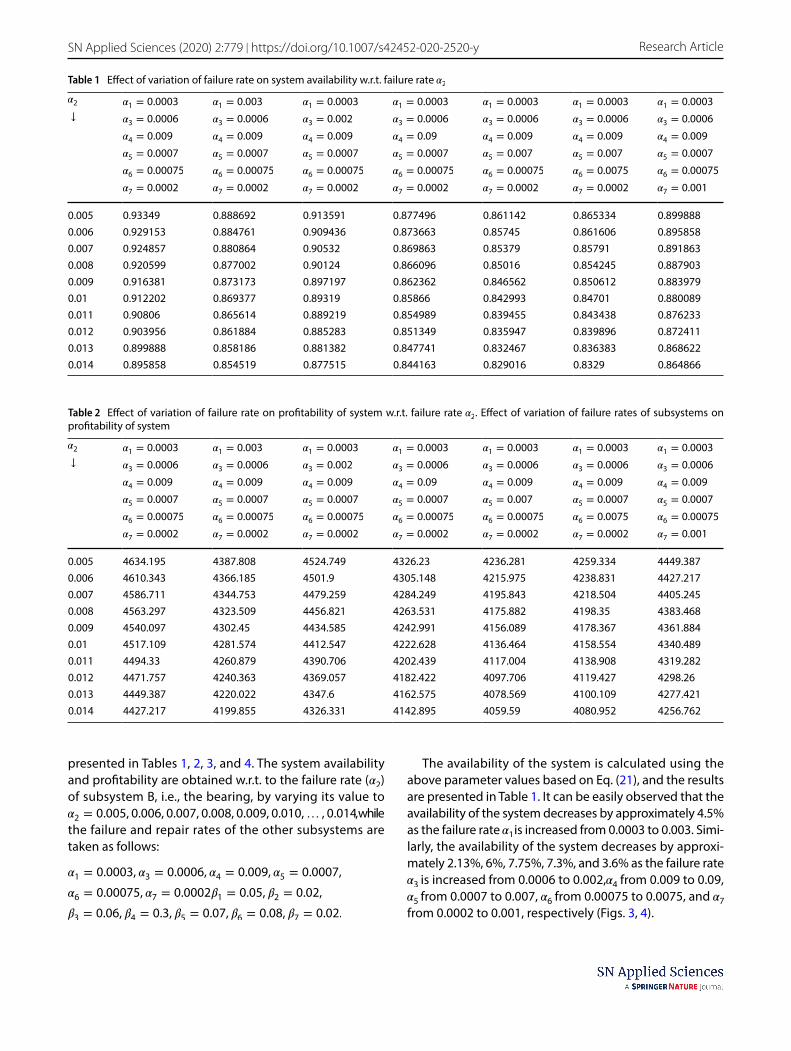
presented in Tables 1, 2, 3, and 4. The system availability and profitability are obtained w.r.t. to the failure rate ( �2 ) of subsystem B, i.e., the bearing, by varying its value to �2 = 0.005, 0.006, 0.007, 0.008, 0.009, 0.010,… , 0.014 , while the failure and repair rates of the other subsystems are taken as follows:

�1 = 0.0003, �3 = 0.0006, �4 = 0.009, �5 = 0.0007,

�6 = 0.00075, �7 = 0.0002�1 = 0.05, �2 = 0.02,

�3 = 0.06, �4 = 0.3, �5 = 0.07, �6 = 0.08, �7 = 0.02.

The availability of the system is calculated using the above parameter values based on Eq. (21), and the results are presented in Table 1. It can be easily observed that the availability of the system decreases by approximately 4.5% as the failure rate �1 is increased from 0.0003 to 0.003. Simi-larly, the availability of the system decreases by approxi-mately 2.13%, 6%, 7.75%, 7.3%, and 3.6% as the failure rate �3 is increased from 0.0006 to 0.002,�4 from 0.009 to 0.09, �5 from 0.0007 to 0.007, �6 from 0.00075 to 0.0075, and �7 from 0.0002 to 0.001, respectively (Figs. 3, 4).

Table 1 Effect of variation of failure rate on system availability w.r.t. failure rate �2�2

↓

�1 = 0.0003

�3 = 0.0006

�4 = 0.009

�5 = 0.0007

�6 = 0.00075

�7 = 0.0002

�1 = 0.003

�3 = 0.0006

�4 = 0.009

�5 = 0.0007

�6 = 0.00075

�7 = 0.0002

�1 = 0.0003

�3 = 0.002

�4 = 0.009

�5 = 0.0007

�6 = 0.00075

�7 = 0.0002

�1 = 0.0003

�3 = 0.0006

�4 = 0.09

�5 = 0.0007

�6 = 0.00075

�7 = 0.0002

�1 = 0.0003

�3 = 0.0006

�4 = 0.009

�5 = 0.007

�6 = 0.00075

�7 = 0.0002

�1 = 0.0003

�3 = 0.0006

�4 = 0.009

�5 = 0.007

�6 = 0.0075

�7 = 0.0002

�1 = 0.0003

�3 = 0.0006

�4 = 0.009

�5 = 0.0007

�6 = 0.00075

�7 = 0.001

0.005 0.93349 0.888692 0.913591 0.877496 0.861142 0.865334 0.8998880.006 0.929153 0.884761 0.909436 0.873663 0.85745 0.861606 0.8958580.007 0.924857 0.880864 0.90532 0.869863 0.85379 0.85791 0.8918630.008 0.920599 0.877002 0.90124 0.866096 0.85016 0.854245 0.8879030.009 0.916381 0.873173 0.897197 0.862362 0.846562 0.850612 0.8839790.01 0.912202 0.869377 0.89319 0.85866 0.842993 0.84701 0.8800890.011 0.90806 0.865614 0.889219 0.854989 0.839455 0.843438 0.8762330.012 0.903956 0.861884 0.885283 0.851349 0.835947 0.839896 0.8724110.013 0.899888 0.858186 0.881382 0.847741 0.832467 0.836383 0.8686220.014 0.895858 0.854519 0.877515 0.844163 0.829016 0.8329 0.864866

Table 2 Effect of variation of failure rate on profitability of system w.r.t. failure rate �2 . Effect of variation of failure rates of subsystems on profitability of system

�2

↓

�1 = 0.0003

�3 = 0.0006

�4 = 0.009

�5 = 0.0007

�6 = 0.00075

�7 = 0.0002

�1 = 0.003

�3 = 0.0006

�4 = 0.009

�5 = 0.0007

�6 = 0.00075

�7 = 0.0002

�1 = 0.0003

�3 = 0.002

�4 = 0.009

�5 = 0.0007

�6 = 0.00075

�7 = 0.0002

�1 = 0.0003

�3 = 0.0006

�4 = 0.09

�5 = 0.0007

�6 = 0.00075

�7 = 0.0002

�1 = 0.0003

�3 = 0.0006

�4 = 0.009

�5 = 0.007

�6 = 0.00075

�7 = 0.0002

�1 = 0.0003

�3 = 0.0006

�4 = 0.009

�5 = 0.0007

�6 = 0.0075

�7 = 0.0002

�1 = 0.0003

�3 = 0.0006

�4 = 0.009

�5 = 0.0007

�6 = 0.00075

�7 = 0.001

0.005 4634.195 4387.808 4524.749 4326.23 4236.281 4259.334 4449.3870.006 4610.343 4366.185 4501.9 4305.148 4215.975 4238.831 4427.2170.007 4586.711 4344.753 4479.259 4284.249 4195.843 4218.504 4405.2450.008 4563.297 4323.509 4456.821 4263.531 4175.882 4198.35 4383.4680.009 4540.097 4302.45 4434.585 4242.991 4156.089 4178.367 4361.8840.01 4517.109 4281.574 4412.547 4222.628 4136.464 4158.554 4340.4890.011 4494.33 4260.879 4390.706 4202.439 4117.004 4138.908 4319.2820.012 4471.757 4240.363 4369.057 4182.422 4097.706 4119.427 4298.260.013 4449.387 4220.022 4347.6 4162.575 4078.569 4100.109 4277.4210.014 4427.217 4199.855 4326.331 4142.895 4059.59 4080.952 4256.762

Vol:.(1234567890)

Research Article SN Applied Sciences (2020) 2:779 | https://doi.org/10.1007/s42452-020-2520-y

Table 3 Effect of variation of repair rate on system availability w.r.t. repair rate �2

�2

↓

�1 = 0.05

�3 = 0.06

�4 = 0.3

�5 = 0.07

�6 = 0.08

�7 = 0.02

�1 = 0.1

�3 = 0.06

�4 = 0.3

�5 = 0.07

�6 = 0.08

�7 = 0.02

�1 = 0.05

�3 = 0.3

�4 = 0.3

�5 = 0.07

�6 = 0.08

�7 = 0.02

�1 = 0.05

�3 = 0.06

�4 = 1.2

�5 = 0.07

�6 = 0.08

�7 = 0.02

�1 = 0.05

�3 = 0.06

�4 = 0.3

�5 = 0.7

�6 = 0.08

�7 = 0.02

�1 = 0.05

�3 = 0.06

�4 = 0.3

�5 = 0.07

�6 = 1.0

�7 = 0.02

�1 = 0.05

�3 = 0.06

�4 = 0.3

�5 = 0.07

�6 = 0.08

�7 = 0.2

0.2 0.93349 0.936112 0.940514 0.934203 0.941399 0.941067 0.9413990.3 0.940809 0.943471 0.947943 0.941533 0.948843 0.948505 0.9488430.4 0.944511 0.947195 0.951702 0.945241 0.952609 0.952269 0.9526090.5 0.946747 0.949443 0.953972 0.94748 0.954883 0.954541 0.9548830.6 0.948243 0.950948 0.955491 0.948979 0.956405 0.956062 0.9564050.7 0.949315 0.952026 0.956579 0.950052 0.957495 0.957152 0.9574950.8 0.95012 0.952836 0.957397 0.950859 0.958314 0.95797 0.9583140.9 0.950747 0.953467 0.958034 0.951487 0.958953 0.958608 0.9589531 0.95125 0.953972 0.958544 0.95199 0.959464 0.959119 0.959464

Table 4 Effect of variation of repair rate on profitability of system w.r.t. repair rate �2

�2

↓

�1 = 0.05

�3 = 0.06

�4 = 0.3

�5 = 0.07

�6 = 0.08

�7 = 0.02

�1 = 0.1

�3 = 0.06

�4 = 0.3

�5 = 0.07

�6 = 0.08

�7 = 0.02

�1 = 0.05

�3 = 0.3

�4 = 0.3

�5 = 0.07

�6 = 0.08

�7 = 0.02

�1 = 0.05

�3 = 0.06

�4 = 1.2

�5 = 0.07

�6 = 0.08

�7 = 0.02

�1 = 0.05

�3 = 0.06

�4 = 0.3

�5 = 0.7

�6 = 0.08

�7 = 0.02

�1 = 0.05

�3 = 0.06

�4 = 0.3

�5 = 0.07

�6 = 1.0

�7 = 0.02

�1 = 0.05

�3 = 0.06

�4 = 0.3

�5 = 0.07

�6 = 0.08

�7 = 0.2

0.2 4634.195 4648.613 4672.825 4638.118 4677.695 4675.868 4677.6950.3 4674.447 4689.093 4713.688 4678.432 4718.635 4716.779 4718.6350.4 4694.811 4709.573 4734.362 4698.828 4739.349 4737.478 4739.3490.5 4707.107 4721.938 4746.846 4711.142 4751.856 4749.976 4751.8560.6 4715.336 4730.214 4755.202 4719.384 4760.228 4758.342 4760.2280.7 4721.23 4736.142 4761.186 4725.287 4766.224 4764.333 4766.2240.8 4725.659 4740.597 4765.683 4729.724 4770.73 4768.836 4770.730.9 4729.109 4744.067 4769.187 4733.179 4774.24 4772.344 4774.241 4731.873 4746.846 4771.993 4735.947 4777.051 4775.153 4777.0511.1 4734.136 4749.122 4774.291 4738.214 4779.353 4777.454 4779.353

Fig. 3 Effect of variation of fail-ure rates on system availability w.r.t. failure rate �2

0.76

0.78

0.8

0.82

0.84

0.86

0.88

0.9

0.92

0.94

0.96

0.005 0.006 0.007 0.008 0.009 0.01 0.011 0.012 0.013 0.014

Avai

labi

lity

Failure rate (α2 )

Variability in availability due to variability in failure rates

no change

change in failure rate ofsubsystem 1

change in failure rate ofsubsystem 3

change in failure rate ofsubsystem 4

change in failure rate ofsubsystem 5

change in failure rate ofsubsystem 6

change in failure rate ofsubsystem 7

Vol.:(0123456789)

SN Applied Sciences (2020) 2:779 | https://doi.org/10.1007/s42452-020-2520-y Research Article

The profitability of the system is calculated using the above dataset, and the results are presented in Table 2. It can be easily observed that the profitability of the system decreases by approximately 5.34% as the failure rate �1 is increased from 0.0003 to 0.003. Similarly, the profit of the system decreases by approximately 2.36%, 6.65%, 8.59%, 8.09%, and 4% when the failure rate �3 is increased from 0.0006 to 0.002, �4 from 0.009 to 0.09, �5 from 0.0007 to 0.007, �6 from 0.00075 to 0.0075, and �7 from 0.0002 to 0.001, respectively.

The system availability and profitability are obtained w.r.t to the repair rate ( �2 ) of subsys-tem  B, i.e., the bearing, by varying its value to �2 = 0.2, 0.3, 0.4, 0.5, 0.6, 0.7, 0.8, 0.9, 1, 1.1 with a constant value of the failure rate �2 = 0.005 . The failure and repair rates of the other subsystems are taken as follows:

The availability of the system is calculated using the above parameter values, and the results are presented in Table 3. It is observed that the availability of the system increases by approximately 0.28% as the repair rate �1 is increased from 0.05 to 0.1. Similarly, the availability of the system increases by approximately 0.75%, 0.08%, 0.85%, 0.81%, and 0.85% as the repair rate �3 is increased from 0.06 to 0.3, �4 from 0.3 to 1.2, �5 from 0.07 to 0.7, �6 from 0.08 to 1, and �7 from 0.02 to 0.2, respectively (Figs. 5, 6).

The profitability of the system is calculated using the fixed set of values, and the results are presented in Table 4.

�1 = 0.0003, �3 = 0.0006, �4 = 0.009, �5 = 0.0007,

�6 = 0.00075, �7 = 0.0002�1 = 0.05, �3 = 0.06,

�4 = 0.3, �5 = 0.07, �6 = 0.08, �7 = 0.02.

Fig. 4 Effect of variation of failure rates on profitability of system w.r.t. failure rate β2

3700

3800

3900

4000

4100

4200

4300

4400

4500

4600

4700

0.005 0.006 0.007 0.008 0.009 0.01 0.011 0.012 0.013 0.014

Profi

t

Failure Rate (α2 )

Change in profit due to change in failure rates

no change

change in failure rate ofsubsystem 1

change in failure rate ofsubsystem 3

change in failure rate ofsubsystem 4

change in failure rate ofsubsystem 5

change in failure rate ofsubsystem 6

change in failure rate ofsubsystem 7

Fig. 5 Effect of variation of repair rates on system avail-ability w.r.t. repair rate �2

0.92

0.925

0.93

0.935

0.94

0.945

0.95

0.955

0.96

0.965

0.2 0.3 0.4 0.5 0.6 0.7 0.8 0.9 1 1.1

Avai

labi

lity

Repair Rate ( β2 )

Variability in Availability due to variability in repair rates

no change

change in repair rate ofsubsystem 1

change in repair rate ofsubsystem 4

change in repair rate ofsubsystem 5

change in repair rate ofsubsystem 6

change in repair rate ofsubsystem 7

Vol:.(1234567890)

Research Article SN Applied Sciences (2020) 2:779 | https://doi.org/10.1007/s42452-020-2520-y

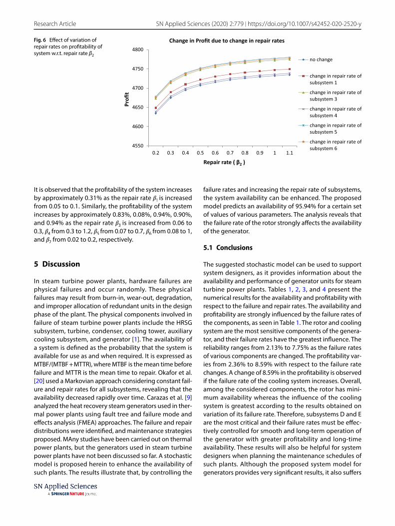
It is observed that the profitability of the system increases by approximately 0.31% as the repair rate �1 is increased from 0.05 to 0.1. Similarly, the profitability of the system increases by approximately 0.83%, 0.08%, 0.94%, 0.90%, and 0.94% as the repair rate �3 is increased from 0.06 to 0.3, �4 from 0.3 to 1.2, �5 from 0.07 to 0.7, �6 from 0.08 to 1, and �7 from 0.02 to 0.2, respectively.

5 Discussion

In steam turbine power plants, hardware failures are physical failures and occur randomly. These physical failures may result from burn-in, wear-out, degradation, and improper allocation of redundant units in the design phase of the plant. The physical components involved in failure of steam turbine power plants include the HRSG subsystem, turbine, condenser, cooling tower, auxiliary cooling subsystem, and generator [1]. The availability of a system is defined as the probability that the system is available for use as and when required. It is expressed as MTBF/(MTBF + MTTR), where MTBF is the mean time before failure and MTTR is the mean time to repair. Okafor et al. [20] used a Markovian approach considering constant fail-ure and repair rates for all subsystems, revealing that the availability decreased rapidly over time. Carazas et al. [9] analyzed the heat recovery steam generators used in ther-mal power plants using fault tree and failure mode and effects analysis (FMEA) approaches. The failure and repair distributions were identified, and maintenance strategies proposed. MAny studies have been carried out on thermal power plants, but the generators used in steam turbine power plants have not been discussed so far. A stochastic model is proposed herein to enhance the availability of such plants. The results illustrate that, by controlling the

failure rates and increasing the repair rate of subsystems, the system availability can be enhanced. The proposed model predicts an availability of 95.94% for a certain set of values of various parameters. The analysis reveals that the failure rate of the rotor strongly affects the availability of the generator.

5.1 Conclusions

The suggested stochastic model can be used to support system designers, as it provides information about the availability and performance of generator units for steam turbine power plants. Tables 1, 2, 3, and 4 present the numerical results for the availability and profitability with respect to the failure and repair rates. The availability and profitability are strongly influenced by the failure rates of the components, as seen in Table 1. The rotor and cooling system are the most sensitive components of the genera-tor, and their failure rates have the greatest influence. The reliability ranges from 2.13% to 7.75% as the failure rates of various components are changed. The profitability var-ies from 2.36% to 8.59% with respect to the failure rate changes. A change of 8.59% in the profitability is observed if the failure rate of the cooling system increases. Overall, among the considered components, the rotor has mini-mum availability whereas the influence of the cooling system is greatest according to the results obtained on variation of its failure rate. Therefore, subsystems D and E are the most critical and their failure rates must be effec-tively controlled for smooth and long-term operation of the generator with greater profitability and long-time availability. These results will also be helpful for system designers when planning the maintenance schedules of such plants. Although the proposed system model for generators provides very significant results, it also suffers

Fig. 6 Effect of variation of repair rates on profitability of system w.r.t. repair rate β2

4550

4600

4650

4700

4750

4800

0.2 0.3 0.4 0.5 0.6 0.7 0.8 0.9 1 1.1

Profi

t

Repair rate ( β2 )

Change in Profit due to change in repair rates

no change

change in repair rate ofsubsystem 1

change in repair rate ofsubsystem 3

change in repair rate ofsubsystem 4

change in repair rate ofsubsystem 5

change in repair rate ofsubsystem 6

Vol.:(0123456789)

SN Applied Sciences (2020) 2:779 | https://doi.org/10.1007/s42452-020-2520-y Research Article

from some limitations, including the use of exponential failure and repair rates and the lack of consideration of simultaneous failures as well as goodness-of-fit analysis of the system availability based on data collected under experimental conditions.

5.2 Future work

In future work, the following issues could be considered:

• Arbitrary distributions for the failure rates of all the sub-systems, e.g., Weibull or Gamma

• Simultaneous occurrence of two or more failures• Goodness-of-fit testing for the availability based on

data for the time to repair and time between failures collected from maintenance records from a plant

Compliance with ethical standards

Conflict of interest The authors declare that they have no conflicts of interest.

References

1. Sabouhia H, Abbaspoura A, Firuzabada MF, Dehghanianb P (2016) Reliability modeling and availability analysis of combined cycle power plants. Electr Power Energy Syst 7:108–119

2. Cox DR (1955) Analysis of non Markovian stochastic processes by the inclusion of supplementary variables. Math Proc Camb Philos Soc 51:433–441

3. Kumar S, Mehta NP, Kumar D (1997) Steady state behavior and maintenance planning of a desulphurization system in urea fer-tilizer plant. Microelectron Reliab 37(6):949–953

4. Arora N, Kumar D (1997) Availability analysis of steam and power generation systems in the thermal power plant. Microelectron Reliab 37(5):795–799

5. Ebeling CE (2000) An introduction to reliability and maintain-ability engineering. Tata Mcgraw Hill, New Delhi

6. Billinton R, Allan RN (2007) Reliability evaluation of engineering systems. Springer, Hyderabad

7. Gupta S, Tewari PC (2009) Simulation modeling and analysis of complex system of thermal power plant. J Ind Eng Manag 2(2):387–406

8. Tewari PC, Kajal S, Khanduja R (2012) Performance evaluation and availability analysis of steam generating system in a thermal power plant. In: Proceedings of the world congress on engineer-ing, p 3

9. Carazas FJG, Salazar CH, Souza GFM (2011) Availability analy-sis of heat recovery steam generators used in thermal power plants. Energy 36(6):3855–3870

10. Balagurusamy E (2011) Reliability engineering. Tata Mcgraw Hill, Hyderabad

11. Adhikarya DD, Bosea GK, Chattopadhyay S, Bosecand D, Mitra S (2012) RAM investigation of coal-fired thermal power plants. Int J Ind Eng Comput 3:423–434

12. Singh VV, Singh SB, Ram M, Goel CK (2013) Availability, MTTF and cost analysis of a system having two units in series configuration with controller. Int J Syst Assur Eng Manag 4(4):341–352

13. Kumar A, Malik SC, Chhillar SK (2016) Analysis of a single-unit system with degradation and maintenance. J Stat Manag Syst 19(2):151–161

14. Kumari R, Sharma AK, Tewari PC (2013) Performance evaluation of a coal-fired power plant. Int J Perform Eng 9(4):455–461

15. Kumar A, Saini M (2018) Analysis of some reliability measures of single unit system subject to abnormal environmental condi-tions and arbitrary distribution for failure and repair activities. J Inf Optim Sci 39(2):545–559

16. Saini M, Kumar A (2019) Performance analysis of evaporation system in sugar industry using RAMD analysis. J Braz Soc Mech Sci Eng 41:4

17. Devi K, Kumar A, Saini M (2017) Performance analysis of a non-identical unit system with priority and Weibull repair and failure laws. Int J Comput Appl 177(7):8–13

18. Suleiman K, Ali UA, Yusuf I (2013) Stochastic analysis and per-formance evaluation of a complex thermal power plant. Innov Syst Softw Eng 4(15):21–31

19. Agarwal SC, Deepika Sharma N (2011) Reliability analysis of sugar manufacturing plant using Boolean function technique. Int J Res Rev Appl Sci 6(2):165–171

20. Okafor CE, Atikpakpa AA, Okonkwo UC (2016) Availability assessment of steam and gas turbine units of a thermal power station using Markovian approach. Arch Curr Res Int 6(4):1–17

21. Aggarwal K, Singh V, Kumar S (2014) Availability analysis and performance optimization of a butter oil production system: a case study. Int J Syst Assur Eng Manag 8(S1):538–554

22. Niwas R, Garg H (2018) An approach for analyzing the reliability and profit of an industrial system based on the cost free war-ranty policy. J Braz Soc Mech Sci Eng 40(5):1–9

23. Kadyan MS, Kumar R (2015) Availability and profit analysis of a feeding system in sugar industry. Int J Syst Assur Eng Manag 8(1):301–316

24. Sabouhi H, Firuzabad M, Dehghanian P (2016) Identifying critical components of combined cycle power plants for implementa-tion of reliability-centered maintenance. CSEE J Power Energy Syst 2(2):87–97

25. Sevsar M (2015) Availability analysis of a power plant by com-puter simulation. Int J Electr Comput Energ Electr Commun Eng 9(4):495–498

26. Kumar A, Saini M (2018) Fuzzy availability analysis of a marine power plant. Mater Today Proc 5(11P3):25195–25202

27. Dahiya O, Kumar A, Saini M (2019) Mathematical modeling and performance evaluation of a-pan crystallization system in a sugar industry. SN Appl Sci. https ://doi.org/10.1007/s4245 2-019-0348-0

Publisher’s Note Springer Nature remains neutral with regard to jurisdictional claims in published maps and institutional affiliations.