Operation and performance of the ATLAS Tile Calorimeter in ...

Eur. Phys. J. C (2018) 78:987https://doi.org/10.1140/epjc/s10052-018-6374-z

Regular Article - Experimental Physics

Operation and performance of the ATLAS Tile Calorimeter inRun 1

ATLAS Collaboration�

CERN, 1211 Geneva 23, Switzerland

Received: 7 June 2018 / Accepted: 29 October 2018 / Published online: 30 November 2018© CERN for the benefit of the ATLAS collaboration 2018

Abstract The Tile Calorimeter is the hadron calorimetercovering the central region of the ATLAS experiment at theLarge Hadron Collider. Approximately 10,000 photomulti-pliers collect light from scintillating tiles acting as the activematerial sandwiched between slabs of steel absorber. Thispaper gives an overview of the calorimeter’s performanceduring the years 2008–2012 using cosmic-ray muon eventsand proton–proton collision data at centre-of-mass energiesof 7 and 8 TeV with a total integrated luminosity of nearly30 fb−1. The signal reconstruction methods, calibration sys-tems as well as the detector operation status are presented.The energy and time calibration methods performed excel-lently, resulting in good stability of the calorimeter responseunder varying conditions during the LHC Run 1. Finally, theTile Calorimeter response to isolated muons and hadrons aswell as to jets from proton–proton collisions is presented. Theresults demonstrate excellent performance in accord withspecifications mentioned in the Technical Design Report.

Contents

1 Introduction . . . . . . . . . . . . . . . . . . . . . 11.1 The ATLAS Tile Calorimeter structure and read-

out electronics . . . . . . . . . . . . . . . . . . 22 Experimental set-up . . . . . . . . . . . . . . . . . 3

2.1 ATLAS experimental data . . . . . . . . . . . . 42.2 Monte Carlo simulations . . . . . . . . . . . . 4

3 Signal reconstruction . . . . . . . . . . . . . . . . . 53.1 Channel time calibration and corrections . . . . 63.2 Electronic noise . . . . . . . . . . . . . . . . . 83.3 Pile-up noise . . . . . . . . . . . . . . . . . . . 10

4 Calibration systems . . . . . . . . . . . . . . . . . 124.1 Caesium calibration . . . . . . . . . . . . . . . 124.2 Laser calibration . . . . . . . . . . . . . . . . . 144.3 Charge injection calibration . . . . . . . . . . . 154.4 Minimum-bias currents . . . . . . . . . . . . . 154.5 Combination of calibration methods . . . . . . 16

� e-mail: [email protected]

5 Data quality analysis and operation . . . . . . . . . 165.1 ATLAS detector control system . . . . . . . . . 165.2 Online data quality assessment and monitoring . 185.3 Offline data quality review . . . . . . . . . . . 185.4 Overall Tile Calorimeter operation . . . . . . . 19

6 Performance studies . . . . . . . . . . . . . . . . . 206.1 Energy response to single isolated muons . . . 20

6.1.1 Cosmic-ray muon data . . . . . . . . . . 216.1.2 Isolated collision muons . . . . . . . . . 24

6.2 Energy response with hadrons . . . . . . . . . 256.2.1 Single hadrons . . . . . . . . . . . . . . 256.2.2 High transverse momentum jets . . . . . 29

6.3 Timing performance with collision data . . . . 316.3.1 Jet analysis . . . . . . . . . . . . . . . . 316.3.2 Muon analysis . . . . . . . . . . . . . . 316.3.3 Combined results . . . . . . . . . . . . . 32

6.4 Summary of performance studies . . . . . . . . 327 Conclusion . . . . . . . . . . . . . . . . . . . . . . 33References . . . . . . . . . . . . . . . . . . . . . . . . 34

1 Introduction

ATLAS [1] is a general-purpose detector designed to recon-struct events from colliding hadrons at the Large Hadron Col-lider (LHC) [2]. The hadronic barrel calorimeter system ofthe ATLAS detector is formed by the Tile Calorimeter (Tile-Cal), which provides essential input to the measurement ofthe jet energies and to the reconstruction of the missing trans-verse momentum. The TileCal, which surrounds the barrelelectromagnetic calorimeter, consists of tiles of plastic scin-tillator regularly spaced between low-carbon steel absorberplates. Typical thicknesses in one period are 3 mm of thescintillator and 14 mm of the absorber parallel to the col-liding beams’ axis, with the steel:scintillator volume ratiobeing 4.7:1. The calorimeter is divided into three longitu-dinal segments; one central long barrel (LB) section with5.8 m in length (|η| < 1.0), and two extended barrel (EB)sections (0.8 < |η| < 1.7) on either side of the barrel each

123

http://crossmark.crossref.org/dialog/?doi=10.1140/epjc/s10052-018-6374-z&domain=pdf

mailto:[email protected]

987 Page 2 of 48 Eur. Phys. J. C (2018) 78 :987

2.6 m long.1 Full azimuthal coverage around the beam axisis achieved with 64 wedge-shaped modules, each covering�φ = 0.1 radians. The Tile Calorimeter is located at an innerradial distance of 2.28 m from the LHC beam-line, and hasthree radial layers with depths of 1.5, 4.1, and 1.8λ (λ standsfor the nuclear interaction length2) for the LB, and 1.5, 2.6,and 3.3λ for the EB. The amount of material in front of theTileCal corresponds to 2.3λ at η = 0 [1]. A detailed descrip-tion of the ATLAS TileCal is provided in a dedicated Tech-nical Design Report [3]; the construction, optical instrumen-tation and installation into the ATLAS detector are describedin Refs. [4,5].

The TileCal design is driven by its ability to reconstructhadrons, jets, and missing transverse momentum within thephysics programme intended for the ATLAS experiment. Forprecision measurements involving the reconstruction of jets,the TileCal is designed to have a stand-alone energy resolu-tion for jets of σ/E = 50%/

√E(GeV) ⊕ 3% [1,3]. To be

sensitive to the full range of energies expected in the LHClifetime, the response is expected to be linear within 2% forjets up to 4 TeV. Good energy resolution and calorimeter cov-erage are essential for precise missing transverse momen-tum reconstruction. A special Intermediate Tile Calorimeter(ITC) system is installed between the LB and EB to correctfor energy losses in the region between the two calorimeters.

This paper presents the performance of the Tile Calorime-ter during the first phase of LHC operation. Section 2describes the experimental data and simulation used through-out the paper. Details of the online and offline signal recon-struction are provided in Sect. 3. The calibration and moni-toring of the approximately 10,000 channels and data acqui-sition system are described in Sect. 4. Section 5 explains thesystem of online and offline data quality checks applied to thehardware and data acquisition systems. Section 6 validatesthe full chain of the TileCal calibration and reconstructionusing events with single muons and hadrons. The perfor-mance of the calorimeter is summarised in Sect. 7.

1.1 The ATLAS Tile Calorimeter structure and read-outelectronics

The light generated in each plastic scintillator is collectedat two edges, and then transported to photomultiplier tubes(PMTs) by wavelength shifting (WLS) fibres [5]. The read-

1 ATLAS uses a right-handed coordinate system with its origin at thenominal interaction point (IP) in the centre of the detector and the z-axisalong the beam pipe. The x-axis points from the IP to the centre of theLHC ring, and the y-axis points upward. Cylindrical coordinates (r, φ)

are used in the transverse plane, φ being the azimuth angle around thez-axis. The pseudorapidity is defined in terms of the polar angle θ asη = − ln tan(θ/2).2 Nuclear interaction length is defined as the mean path length to reducethe flux of relativistic primary hadrons to a fraction 1/e.

out cell geometry is defined by grouping the fibres from indi-vidual tiles on the corresponding PMT. A typical cell is readout on each side (edge) by one PMT, each corresponding toone channel. The dimensions of the cells are �η × �φ =0.1×0.1 in the first two radial layers, called layers A and BC(just layer B in the EB), and �η×�φ = 0.2×0.1 in the thirdlayer, referred to as layer D. The projective layout of cellsand naming convention are shown in Fig. 1. The so-calledITC cells (D4, C10 and E-cells) are located between the LBand EB, and provide coverage in the range 0.8 < |η| < 1.6.Some of the C10 and D4 cells have reduced thickness or spe-cial geometry in order to accommodate services and read-out electronics for other ATLAS detector systems [3,6]. Thegap (E1–E2) and crack (E3–E4) cells are only composed ofscintillator and are exceptionally read out by only one PMT.For Run 1, eight crack scintillators were removed per side,to allow for routing of fibres for 16 Minimum Bias TriggerScintillators (MBTS), used to trigger on events from collid-ing particles, as well as to free up the necessary electronicschannels for read-out of the MBTS. The MBTS scintillatorsare also read out by the TileCal EB electronics.

The PMTs and front-end electronics are housed in a steelgirder at the outer radius of each module in 1.4 m long alu-minium units that can be fully extracted while leaving theremaining module in place, and hence are given the nameof electronics drawers. Each drawer holds a maximum of 24channels, two of which form a super-drawer. There are nom-inally 45 and 32 active channels per super-drawer in the LBand EB, respectively. Each channel consists of a unit calleda PMT block, which contains the light-mixer, PMT tube andvoltage divider, and a so-called 3-in-1 card [7,8]. This cardis responsible for fast signal shaping in two gains (with abi-gain ratio of 1:64), the slow integration of the PMT sig-nal, and provides an input for a charge injection calibrationsystem.

The maximum height of the analogue pulse in a channel isproportional to the amount of energy deposited by the inci-dent particle in the corresponding cell. The shaped signalsare sampled and digitised every 25 ns by 10-bit ADCs [9].The sampled data are temporarily stored in a pipeline mem-ory until a trigger Level-1 signal is received. Seven samples,centred around the pulse peak, are obtained. A gain switch isused to determine which gain information is sent to the back-end electronics for event processing. By default the high-gainsignal is used, unless any of the seven samples saturates theADC, at which point the low-gain signal is transmitted.

Adder boards receive the analogue low-gain signal fromthe 3-in-1 cards and sum the signal from six 3-in-1 cardswithin �η × �φ = 0.1 × 0.1 before transmitting it to theATLAS hardware-based trigger system as a trigger tower.

The integrator circuit measures PMT currents (0.01 nAto 1.4µA) over a long time window of 10–20 ms with oneof the six available gains, and is used for calibration with

123

Eur. Phys. J. C (2018) 78 :987 Page 3 of 48 987

500 1000 1500 mm0

A3 A4 A5 A6 A7 A8 A9 A10A1 A2

BC1 BC2 BC3 BC5 BC6 BC7 BC8BC4

D0 D1 D2 D3

A13 A14 A15 A16

B9

B12 B14 B15

D5 D6D4

C10

0,7 1,0 1,1

1,3

1,4

1,5

1,6

B11 B13

A12

E4

E3

E2

E1

beam axis

0,1 0,2 0,3 0,4 0,5 0,6 0,8 0,9 1,2

2280 mm

3865 mm=0,0η

~~

Fig. 1 The layout of the TileCal cells, denoted by a letter (A to E) plus an integer number. The A-layer is closest to the beam-line. The namingconvention is repeated on each side of η = 0

a radioactive caesium source and to measure the rate of softinteractions during collisions at the LHC [10]. It is a low-passDC amplifier that receives less than 1% of the PMT current,which is then digitised by a 12-bit ADC card (which saturatesat 5 V) [11].

Power is supplied to the front-end electronics of a sin-gle super-drawer by means of a low-voltage power supply(LVPS) source, which is positioned in an external steel boxmounted just outside the electronics super-drawer. The highvoltage is set and distributed to each individual PMT usingdedicated boards positioned inside the super-drawers locatedwith the front-end electronics.

The back-end electronics is located in a counting roomapproximately 100 m away from the ATLAS detector. Thedata acquisition system of the Tile Calorimeter is split intofour partitions, the ATLAS A-side (η > 0) and C-side(η < 0) for both the LB and EB, yielding four logical par-titions: LBA, LBC, EBA, and EBC. Optical fibres transmitsignals between each super-drawer and the back-end trigger,timing and control (TTC) and read-out driver (ROD [12])crates. There are a total of four TTC and ROD crates, onefor each physical partition. The ATLAS TTC system dis-tributes the LHC clock, trigger decisions, and configurationcommands to the front-end electronics. If the TTC systemsends the trigger acceptance command to the front-end elec-tronics, the corresponding digital signals for all channels ofthe calorimeter are sent to the ROD via optical links, wherethe signal is reconstructed for each channel.

2 Experimental set-up

The data used in this paper were taken by the Tile Calorimetersystem using the full ATLAS data acquisition chain. In addi-tion to the TileCal, there are also other ATLAS subsystemsused to assist in particle identification, track, momentum,and energy reconstruction. The inner detector is composedof a silicon pixel detector (Pixel), a semiconductor tracker(SCT), and a transition radiation tracker (TRT). Together theyprovide tracking of charged particles for |η| < 2.5, with adesign resolution of σpT/pT = 0.05% · pT(GeV) ⊕ 1% [1].The electromagnetic lead/liquid-argon barrel (EMB [13])and endcap (EMEC [14]) calorimeters provide coveragefor |η| < 3.2. The energy resolution of the liquid-argon(LAr) electromagnetic calorimeter is designed to be σE/E =10%/

√E(GeV) ⊕ 0.7%. The hadronic calorimetry in the

central part of the detector (|η| < 1.7) is provided by theTileCal, which is described in detail in Sect. 1. In the endcapregion (1.5 < |η| < 3.2) hadronic calorimetry is providedby a LAr/copper sampling calorimeter (HEC [15]) behind aLAr/lead electromagnetic calorimeter with accordion geom-etry, while in the forward region (3.2 < |η| < 4.9) theFCal [16] provides electromagnetic (the first module withLAr/copper) and hadronic (the second and third module withLAr/tungsten) calorimetry. The muon spectrometer system,the outermost layer of the ATLAS detector, is composed ofmonitored drift tubes, and cathode strip chambers for the end-cap muon track reconstruction for |η| < 2.7. Resistive platechambers (RPCs) and thin gap chambers (TGCs) are usedto trigger muons in the range |η| < 2.4. ATLAS has foursuperconducting magnet systems. In the central region, a 2 Tsolenoid placed between the inner detector and calorimetersis complemented with 0.5 T barrel toroid magnets located

123


Table 1 Summary of protoncollision data presented in thispaper. The ATLAS analysisintegrated luminositycorresponds to the totalintegrated luminosity approvedfor analysis, passing all dataquality requirements ensuringthe detector and reconstructionsoftware is properly functioning.The maximum and the average(listed in parentheses) of thedistribution of the mean numberof interactions per bunchcrossing are given

2010 2011 2012

Maximum beam energy (TeV) 3.5 3.5 4

Delivered integrated luminosity 48.1 pb−1 5.5 fb−1 22.8 fb−1

ATLAS analysis integrated luminosity 45.0 pb−1 4.7 fb−1 20.3 fb−1

Minimum bunch spacing (ns) 150 50a 50a

Maximum number of bunches 348 1331b 1380

Mean number of interactions per bunch crossing 4 (1) 17 (9) 36 (20)

Maximum instantaneous luminosity (1033 cm−2s−1) 0.2 3.8 7.5

aAdditional special runs with low integrated luminosity used for commissioning purposes were taken with aminimal bunch spacing of 25 nsbAdditional special runs were taken with low integrated luminosity where the number of colliding buncheswas increased to 1842 in 2011

outside of TileCal. Both endcap regions encompass their owntoroid magnet placed between TileCal and muon system, pro-ducing the field of 1.0 T.

A three-level trigger system [17] was used by ATLAS inRun 1 to reduce the event rate from a maximum raw rateof 40 MHz to 200 Hz, which is written to disk. The Level 1Trigger (L1) is a hardware-based decision using the energycollected in coarse regions of the calorimeter and hits in themuon spectrometer trigger system. The High Level Trigger(HLT) is composed of the Level 2 Trigger (L2) and the EventFilter (EF). The HLT uses the full detector information inthe regions of interest defined by L1. The reconstruction isfurther refined in going from L2 to the EF, with the EF usingthe full offline reconstruction algorithms. A trigger chain isdefined by the sequence of algorithms used in going from L1to the EF. Events passing trigger selection criteria are sepa-rated into different streams according to the trigger categoryfor which the event is triggered. Physics streams are com-posed of triggers that are used to identify physics objects(electrons, photons, muons, jets, hadronically-decaying τ -leptons, missing transverse momentum) in collision data.There are also calibration streams used by the various sub-systems for calibration and monitoring purposes, which takedata during empty bunch crossings in collision runs or indedicated calibration runs. Empty bunch crossings are thosewith no proton bunch and are separated from any filled bunchby at least five bunch crossings to ensure signals from col-lision events are cleared from the detector. The calibrationand monitoring data are explained in more detail in the nextsections.

2.1 ATLAS experimental data

The full ATLAS detector started recording events fromcosmic-ray muons in 2008 as a part of the detector com-missioning [6,18]. Cosmic-ray muon data from 2008–2010are used to validate test beam and in situ calibrations, and to

study the full calorimeter in the ATLAS environment; theseresults are presented in Sect. 6.1.1.

The first√s = 7 TeV proton–proton (pp) collisions were

recorded in March 2010, and started a rich physics pro-gramme at the LHC. In 2011 the LHC pp collisions con-tinued to be at

√s = 7 TeV, but the instantaneous luminosity

increased and the bunch spacing decreased to 50 ns. Mov-ing to 2012 the centre-of-mass energy increased to 8 TeV.In total, nearly 30 fb−1 of proton collision data were deliv-ered to ATLAS during Run 1. A summary of the LHC beamconditions is shown in Table 1 for 2010–2012, representingthe collision data under study in this paper. In ATLAS, datacollected over long periods of time spanning an LHC fill orgenerally stable conditions are grouped into a “run”, whilethe entire running period under similar conditions for severalyears is referred to as a “Run”. Data taken within a run arebroken down into elementary units called luminosity blocks,corresponding to up to one minute of collision data for whichdetector conditions or software calibrations remain approxi-mately constant.

ATLAS also recorded data during these years with lower-energy proton collisions (at

√s = 900 GeV, 2.76 TeV), and

data containing lead ion collisions. Nevertheless, this paperfocuses on the results obtained in pp collisions at

√s = 7

and 8 TeV.

2.2 Monte Carlo simulations

Monte Carlo (MC) simulated data are frequently used by per-formance and physics groups to predict the behaviour of thedetector. It is crucial that the MC simulation closely matchesthe actual data, so those relying on simulation for algorithmoptimisations and/or searches for new physics are not misledin their studies.

The MC process is divided into four steps: event gener-ation, simulation, digitisation, and reconstruction. Variousevent generators were used in the analyses as described ineach subsection. The ATLAS MC simulation [19] relies on

123


the Geant4 toolkit [20] to model the detector and interac-tions of particles with the detector material. During Run 1,ATLAS used the so-called QGSP_BERT physics model todescribe the hadronic interactions with matter, where at highenergies the hadron showers are modelled using the GluonString Plasma model, and the Bertini intra-nuclear cascademodel is used for lower-energy hadrons [21]. The input tothe digitisation is a collection of hits in the active scintilla-tor material, characterised by the energy, time, and position.The amount of energy deposited in scintillator is dividedby the calorimeter sampling fraction to obtain the channelenergy [22]. In the digitisation step, the channel energy inGeV is converted into its equivalent charge using the elec-tromagnetic scale constant (Sect. 4) measured in the beamtests. The charge is subsequently translated into the signalamplitude in ADC counts using the corresponding calibra-tion constant (Sect. 4.3). The amplitude is convolved withthe pulse shape and digitised each 25 ns as in real data. Theelectronic noise is emulated and added to the digitised sam-ples as described in Sect. 3.2. Pile-up (i.e. contributions fromadditional minimum-bias interactions occurring in the samebunch crossing as the hard-scattering collision or in nearbyones), are simulated with Pythia 6 [23] in 2010–2011 andPythia 8 [24] in 2012, and mixed at realistic rates withthe hard-scattering process of interest during the digitisa-tion step. Finally, the same reconstruction methods, detailedin Sect. 3, as used for the data are applied to the digitisedsamples of the simulations.

3 Signal reconstruction

The electrical signal for each TileCal channel is reconstructedfrom seven consecutive digital samples, taken every 25 ns.Nominally, the reconstruction of the signal pulse amplitude,time, and pedestal is made using the Optimal Filtering (OF)technique [25]. This technique weights the samples in accor-dance with a reference pulse shape. The reference pulse shapeused for all channels is taken as the average pulse shape fromtest beam data, with reference pulses for both high- and low-gain modes, each of which is shown in Fig. 2. The signalamplitude (A), time phase (τ ), and pedestal (p) for a channelare calculated using the ADC count of each sample Si takenat time ti :

A =n=7∑

i=1

ai Si , Aτ =n=7∑

i=1

bi Si , p =n=7∑

i=1

ci Si (1)

where the weights (ai , bi , and ci ) are derived to minimise theresolution of the amplitude and time, with a set of weightsextracted for both high and low gain. Only electronic noisewas considered in the minimisation procedure in Run 1.

Time [ns]

-60 -40 -20 0 20 40 60 80 100 120

Nor

mal

ised

sig

nal h

eigh

t

0

0.2

0.4

0.6

0.8

1 Low gain

High gainATLAS

Fig. 2 The reference pulse shapes for high gain and low gain, shownin arbitrary units [6]

The expected time of the pulse peak is calibrated suchthat for particles originating from collisions at the interactionpoint the pulse should peak at the central (fourth) sample,synchronous with the LHC 40 MHz clock. The reconstructedvalue of τ represents the small time phase in ns between theexpected pulse peak and the time of the actual reconstructedsignal peak, arising from fluctuations in particle travel timeand uncertainties in the electronics read-out.

Two modes of OF reconstruction were used during Run 1,an iterative and a non-iterative implementation. In the itera-tive method, the pulse shape is recursively fit when the dif-ference between maximum and minimum sample is above anoise threshold. The initial time phase is taken as the timeof the maximum sample, and subsequent steps use the pre-vious time phase as the starting input for the fit. Only oneiteration is performed assuming a pulse with the peak inthe central sample for signals below a certain threshold. Forevents with no out-of-time pile-up (see Sect. 3.3) this iterativemethod proves successful in reconstructing the pulse peaktime to within 0.5 ns. This method is used when reconstruct-ing events occurring asynchronously with the LHC clock,such as cosmic-ray muon data and also to reconstruct datafrom the 2010 proton collisions. With an increasing numberof minimum-bias events per bunch crossing, the non-iterativemethod, which is more robust against pile-up, is used. Thetime phase was fixed for each individual channel and only asingle fit to the samples was applied in 2011–2012 data.

In real time, or online, the digital signal processor (DSP)in the ROD performs the signal reconstruction using the OFtechnique, and provides channel energy and time to the HLT.The conversion between signal amplitude in ADC counts andenergy units of MeV is done by applying channel-dependentcalibration constants which are described in the next sec-tion. The DSP reconstruction is limited by the use of fixed

123


[ns]DSPt

−25 −20 −15 −10 −5 0 5 10 15 20 25

[%]

OF

LIE

)/O

FLI

E-D

SP

E(

−40

−35

−30

−25

−20

−15

−10

−5

0

5

10

OF Online

OF Online + Phase Correction

ATLAS

=7 TeV 2011 datas

Fig. 3 The relative difference between the online channel energy(EDSP) calculated using the non-iterative OF method and the offline(EOFLI) channel energy reconstruction using the iterative OF method,as a function of the phase computed by the DSP (tDSP) with no correction(circles) and with application of the parabolic correction (squares) as afunction of phase (τ ). The error bars are the standard deviations (RMS)of the relative difference distribution. Data are shown for collisions in2011

point arithmetic, which has a precision of 0.0625 ADC counts(approximately 0.75 MeV in high gain), and imposes preci-sion limitations for the channel-dependent calibration con-stants.

The offline signal is reconstructed using the same iterativeor non-iterative OF technique as online. In 2010 the raw datawere transmitted from the ROD for offline signal reconstruc-tion, and the amplitude and time computations from the RODwere used only for the HLT decision. From 2011 onward,with increasing instantaneous luminosity the output band-width of the ROD becomes saturated, and only channels forwhich the difference between the maximum and minimumSi is larger than five ADC counts (approximately 60 MeV)have the raw data transmitted from the ROD for the offlinesignal reconstruction; otherwise the ROD signal reconstruc-tion results are used for the offline data processing.

The reconstructed phase τ is expected to be small, but forany non-zero values of the phase, there is a known bias whenthe non-iterative pulse reconstruction is used that causesthe reconstructed amplitude to be underestimated. A correc-tion based on the phase is applied when the phase is recon-structed within half the LHC bunch spacing and the channelamplitude is larger than 15 ADC counts, to reduce contribu-tions from noise. Figure 3 shows the difference between thenon-iterative energy reconstructed in the DSP without (cir-cles) and with (squares) this parabolic correction, relative tothe iterative reconstruction calculated offline for data takenduring 2011. Within time phases of ± 10 ns the differencebetween the iterative and non-iterative approaches with theparabolic correction applied is less than 1%.

The difference between the energies reconstructed usingthe non-iterative (with the parabolic correction applied) and

[MeV]OFLNIE0 200 400 600 800 1000 1200 1400

[MeV

]O

FLI

-EO

FLN

IE

-100

-50

0

50

100

0

20

40

60

80

100

120

140

160

180

200

220ATLAS

=7 TeV 2010 datas

Fig. 4 The absolute difference between the energies reconstructedusing the optimal filtering reconstruction method with the non-iterative(EOFLNI) and iterative (EOFLI) signal reconstruction methods as a func-tion of energy. The black markers represent mean values of EOFLNI–EOFLI per a bin of EOFLNI. The parabolic correction is applied toEOFLNI. The data shown uses high pT (> 20 GeV) isolated muonsfrom

√s = 7 TeV collisions recorded in 2010

iterative OF technique as a function of energy can be seenin Fig. 4 for high pT (> 20 GeV) isolated muons taken fromthe 2010

√s = 7 TeV collision data. For channel energies

between 200 and 400 MeV the mean difference between thetwo methods is smaller than 10 MeV. For channel energieslarger than 600 MeV, the mean reconstructed energy is thesame for the two methods.

3.1 Channel time calibration and corrections

Correct channel time is essential for energy reconstruction,object selection, and for time-of-flight analyses searchingfor hypothetical long-lived particles entering the calorimeter.Initial channel time calibrations are performed with laser andcosmic-ray muon events, and are later refined using beam-splash events from a single LHC beam [6]. A laser calibrationsystem pulses laser light directly into each PMT. The systemis used to calibrate the time of all channels in one super-drawer such that the laser signal is sampled simultaneously.These time calibrations are used to account for time delaysdue to the physical location of the electronics. Finally, thetime calibration is set with collision data, considering in eachevent only channels that belong to a reconstructed jet. Thisapproach mitigates the bias from pile-up noise (Sect. 3.3)and non-collision background. Since the reconstructed timeslightly depends on the energy deposited by the jet in a cell(Fig. 5 left), the channel energy is further required to be in acertain range (2–4 GeV) for the time calibration. An exam-ple of the reconstructed time spectrum in a channel satisfyingthese conditions is shown in Fig. 5(right). The distributionshows a clear Gaussian core (the Gaussian mean determinesthe time calibration constant) with a small fraction of events

123


Cell energy [GeV]1 10

⟨ Cel

l tim

e [

ns]

⟩

-2

-1

0

1

2

3

4 Data, Jets

bandσ1*

ATLAS

=7 TeV, 50 ns, 2011s

Channel time [ns]

−10 −8 −6 −4 −2 0 2 4 6 8 10

Ent

ries/

0.5

ns

−110

1

10

210

310

410ATLAS = 7 TeVs

50 ns, 2011

Fig. 5 Left: the mean cell reconstructed time (average of the timesin the two channels associated with the given cell) as measured withjet events. The mean cell time decreases with the increase of the cellenergy due to the reduction of the energy fraction of the slow hadronic

component of hadronic showers [26,27]. Right: example of the channelreconstructed time in jet events in 2011 data, with the channel energybetween 2 and 4 GeV. The solid line represents the Gaussian fit to thedata

at both high- and low-time tails. The higher-time tails aremore evident for low-energy bins and are mostly due to theslow hadronic component of the shower development. Sym-metric tails are due to out-of-time pile-up (see Sect. 3.3) andare not seen in 2010 data where pile-up is negligible. Theoverall time resolution is evaluated with jets and muons fromcollision data, and is described in Sect. 6.3.

During Run 1 a problem was identified in which a digi-tiser could suddenly lose its time calibration settings. Thisproblem, referred to as a “timing jump”, was later traced tothe TTCRx chip in the digitiser board, which received clockconfiguration commands responsible for aligning that digi-tiser sampling clock with the LHC clock. During operationthese settings are sent to all digitisers during configurationof the super-drawers, so a timing jump manifests itself at thebeginning of a run or after a hardware failure requiring recon-figuration during a run. All attempts to avoid this feature atthe hardware or configuration level failed, hence the detectionand correction of faulty time settings became an importantissue. Less than 15% of all digitisers were affected by thesetiming jumps, and were randomly distributed throughout theTileCal. All channels belonging to a given digitiser exhibitthe same jump, and the magnitude of the shift for one digitiseris the same for every jump.

Laser and collision events are used to detect and correctfor the timing jumps. Laser events are recorded in parallelto physics data in empty bunch crossings. The reconstructedlaser times are studied for each channel as a function of lumi-

nosity block. As the reconstructed time phase is expected tobe close to zero the monitoring algorithm searches for differ-ences (> 3 ns) from this baseline. Identified cases are classi-fied as potential timing jumps, and are automatically reportedto a team of experts for manual inspection. The timing dif-ferences are saved in the database and applied as a correctionin the offline data reconstruction.

Reconstructed jets from collision data are used as a sec-ondary tool to verify timing jumps, but require completionof the full data reconstruction chain and constitute a smallersample as a function of luminosity block. These jets are usedto verify any timing jumps detected by the laser analysis, orused by default in cases where the laser is not operational.For the latter, problematic channels are identified after thefull reconstruction, but are corrected in data reprocessingcampaigns.

A typical case of a timing jump is shown in Fig. 6 before(left) and after (right) the time correction. Before the correc-tion the time step is clearly visible and demonstrates goodagreement between the times measured by the laser andphysics collision data.

The overall impact of the timing jump corrections on thereconstructed time is studied with jets using 1.3 fb−1 of col-lision data taken in 2012. To reduce the impact of the timedependence on the reconstructed energy, the channel energyis required to be E > 4 GeV, and read out in high-gain mode.The results are shown in Fig. 7, where the reconstructedtime is shown for all calorimeter channels with and without

123


Luminosity Block

[ns]

chan

nel

t

−30

−20

−10

0

10

20

30

LBC55, ch 28Physics dataLaser

Run 212199,before correction

ATLAS

Luminosity Block

100 200 300 400 500 600 100 200 300 400 500 600

[ns]

chan

nel

t

−30

−20

−10

0

10

20

30

LBC55, ch 28Physics data

Run 212199,after correction

ATLAS

Fig. 6 An example of timing jumps detected using the laser (full redcircles) and physics (open black circles) events (left) before and (right)after the correction. The small offset of about 2 ns in collision data is

caused by the energy dependence of the reconstructed time in jet events(see Fig. 5, left). In these plots, events with any energy are accepted toaccumulate enough statistics

[ns]channelt

−30 −20 −10 0 10 20

Ent

ries

/ 0.5

ns

1

10

210

310

410

510

610 ATLAS

No correction

Corrected

Fig. 7 Impact of the timing jump corrections on the reconstructedchannel time in jets from collision data. Shown are all high-gain chan-nels with Ech > 4 GeV associated with a reconstructed jet. The plotrepresents 1.3 fb−1 of pp collision data acquired in 2012

the timing jump correction. While the Gaussian core, corre-sponding to channels not affected by timing jumps, remainsbasically unchanged, the timing jump correction significantlyreduces the number of events in the tails. The 95% quantilerange around the peak position shrinks by 12% (from 3.3 ns to2.9 ns) and the overall RMS improves by 9% (from 0.90 nsto 0.82 ns) after the corrections are applied. In preparationfor Run 2, problematic digitisers were replaced and repaired.The new power supplies, discussed in the next section, alsocontribute to the significant reduction in the number of the

timing jumps since the trips almost ceased (Sect. 5.4) and thusthe module reconfigurations during the run are eliminated inRun 2.

3.2 Electronic noise

The total noise per cell is calculated taking into account twocomponents, electronic noise and a contribution from pile-up interactions (so-called pile-up noise). These two contri-butions are added in quadrature to estimate the total noise.Since the cell noise is directly used as input to the topologicalclustering algorithm [28] (see Sect. 6), it is very important toestimate the noise level per cell with good precision.

The electronic noise in the TileCal, measured by fluctua-tions of the pedestal, is largely independent of external LHCbeam conditions. Electronic noise is studied using large sam-ples of high- and low-gain pedestal calibration data, whichare taken in dedicated runs without beam in the ATLAS detec-tor. Noise reconstruction of pedestal data mirrors that of thedata-taking period, using the OF technique with iterations for2010 data and the non-iterative version from 2011 onward.

The electronic noise per channel is calculated as a stan-dard deviation (RMS) of the energy distributions in pedestalevents. The fluctuation of the digital noise as a function oftime is studied with the complete 2011 dataset. It fluctuatesby an average of 1.2% for high gain and 1.8% for low gainacross all channels, indicating stable electronic noise con-stants.

As already mentioned in Sect. 1.1, a typical cell is readout by two channels. Therefore, the cell noise constants arederived for the four combinations of the two possible gains

123


η-1.5 -1 -0.5 0 0.5 1 1.5

Ele

ctro

nic

Noi

se [M

eV]

20

40

60

High Gain - High Gain

2011 ATLAS RUN I Reprocessing

ATLASA Cells

BC Cells

D Cells

E Cells

Fig. 8 The φ-averaged electronic noise (RMS) as a function of η ofthe cell, with both contributing read-out channels in high-gain mode.For each cell the average value over all modules is taken. The statisti-cal uncertainties are smaller than the marker size. Values are extractedusing all the calibration runs used for the 2011 data reprocessing. Thedifferent cell types are shown separately for each layer: A, BC, D, andE (gap/crack). The transition between the long and extended barrels canbe seen in the range 0.7 < |η| < 1.0

from the two input channels (high–high, high–low, low–high,and low–low). Figure 8 shows the mean cell noise (RMS) forall cells as a function of η for the high–high gain combi-nations. The figure also shows the variations with cell type,reflecting the variation with the cell size. The average cellnoise is approximately 23.5 MeV. However, cells located inthe highest |η| ranges show noise values closer to 40 MeV.These cells are formed by channels physically located nearthe LVPS. The influence of the LVPS on the noise distributionis discussed below. A typical electronic noise values for othercombinations of gains are 400–700 MeV for high–low/low–high gain combinations and 600–1200 MeV for low–low gaincase. Cells using two channels with high gain are relevantwhen the deposited energy in the cell is below about 15 GeV,above that both channels are often in low-gain mode, andif they fall somewhere in the middle range of energies (10–20 GeV) one channel is usually in high gain and the other inlow gain.

During Run 1 the electronic noise of a cell is best describedby a double Gaussian function, with a narrow central singleGaussian core and a second central wider Gaussian func-tion to describe the tails [6]. A normalised double Gaussiantemplate with three parameters (σ1, σ2, and the relative nor-malisation of the two Gaussian functions R) is used to fit theenergy distribution:

fpdf = 1

1 + R

(1√

2πσ1e− x2

2σ21 + R√

2πσ2e− x2

2σ22

)

The means of the two Gaussian functions are set toμ1 = μ2 = 0, which is a good approximation for the cellnoise. As input to the topological clustering algorithm an

Fig. 9 Ratio of the RMS to the width (σ ) of a single Gaussian fitto the electronic noise distribution for all channels averaged over 40TileCal modules before (squares) and after (circles) the replacement ofthe LVPS. Higher-number channels are closer to the LVPS

equivalent σeq(E) is introduced to measure the significance(S = |E |/σeq(E)) of the double Gaussian probability distri-bution function in units of standard deviations of a normaldistribution.3

The double Gaussian behaviour of the electronic noiseis believed to originate from the LVPS used during Run 1,as the electronic noise in test beam data followed a singleGaussian distribution, and this configuration used tempo-rary power supplies located far from the detector. DuringDecember 2010, five original LVPS sources were replacedby new versions of the LVPS. During operation in 2011 theseLVPSs proved to be more reliable by suffering virtually notrips, and resulted in lower and more single-Gaussian-likebehaviour of channel electronic noise. With this success, 40more new LVPS sources (corresponding to 16% of all LVPSs)were installed during the 2011–2012 LHC winter shutdown.Figure 9 shows the ratio of the RMS to the width of a sin-gle Gaussian fit to the electronic noise distribution for allchannels averaged over the 40 modules before and after thereplacement of the LVPS. It can be seen that the new LVPShave values of RMS/σ closer to unity, implying a shape sim-ilar to a single Gaussian function, across all channels. Theaverage cell noise in the high–high gain case decreases to20.6 MeV with the new LVPS.

The coherent component of the electronic noise was alsoinvestigated. A considerable level of correlation was onlyfound among channels belonging to the same motherboard,4

3 The σeq(E) defines the region where the significance for the doubleGaussian fpdf is the same as in the 1σ region of a standard Gaussiandistribution function, i.e. 1σeq(E) is defined as

∫ σeq−σeq

fpdf dx = 0.68,

2σeq(E) as∫ 2σeq−2σeq

fpdf dx = 0.954, etc.4 Each motherboard accommodates 12 consecutive channels in a super-drawer. One of its roles is to distribute the low voltages to the electroniccomponents of individual channels [7].

123


Tile Cell Energy [GeV]

-1 0 1 2 3 4 5

/ dE

/ 0.

06 G

eVce

llsdN

-510

-410

-310

-210

-110

1

10

210

310

410

EMScale

ATLAS= 7TeVsMinBias MC,

= 7 TeVsData,

= 2.36TeVsData,

= 0.9 TeVsData,

Random Trigger

Fig. 10 The TileCal cell energy spectrum at the electromagnetic (EM)scale measured in 2010 data. The distributions from collision data at7 TeV, 2.36 TeV, and 0.9 TeV are superimposed with Pythia minimum-bias Monte Carlo and randomly triggered events

for other pairs of channels the correlations are negligible.Methods to mitigate the coherent noise were developed;5 theyreduce the correlations from (− 40%, + 70%) to (− 20%,+ 10%) and also decrease the fraction of events in the tailsof the double Gaussian noise distribution.Electronic noise in the Monte Carlo simulations

The emulation of the electronic noise, specific to eachindividual calorimeter cell, is implemented in the digitisationof the Monte Carlo signals. It is assumed that it is possibleto convert the measured cell noise to an ADC noise in thedigitisation step, as the noise is added to the individual sam-ples in the MC simulation. The correlations between the twochannels in the cell are not considered. As a consequence,the constants of the double Gaussian function, used to gen-erate the electronic noise in the MC simulation, are derivedfrom the cell-level constants used in the real data. As a clo-sure test, after reconstruction of the cell energies in the MCsimulation the cell noise constants are calculated using thesame procedure as for real data. The reconstructed cell noisein the MC reconstruction is found to be in agreement withthe original cell noise used as input from the real data. Goodagreement between data and MC simulation of the energy ofthe TileCal cells, also for the low and negative amplitudes,is found (see Fig. 10). The measurement is performed using2010 data where the pile-up contribution is negligible. Thenoise contribution can be compared with data collected usinga random trigger.

5 The first method estimated the coherent component of the noise as anaverage over all channels in the same motherboard with signals less than3× the electronic noise variation; this average value was then used tocorrect the individual channel energies provided at least 60% of channelscontributed to the calculation. The second method [29] is based on theχ2 minimisation.

3.3 Pile-up noise

The pile-up effects consist of two contributions, in-time pile-up and out-of-time pile-up. The in-time pile-up originatesfrom multiple interactions in the same bunch crossing. Incontrast, the out-of-time pile-up comes from minimum-biasevents from previous or subsequent bunch crossings. The out-of-time pile-up is present if the width of the electrical pulse(Fig. 2) is longer than the bunch spacing, which is the casein Run 1 where the bunch spacing in runs used for physicsanalyses is 50 ns. These results are discussed in the followingparagraphs.

The pile-up in the TileCal is studied as a function ofthe detector geometry and the mean number of inelasticpp interactions per bunch crossing 〈μ〉 (averaged over allbunch crossings within a luminosity block and depending onthe actual instantaneous luminosity and number of collid-ing bunches). The data are selected using a zero-bias trigger.This trigger unconditionally accepts events from collisionsoccurring a fixed number of LHC bunch crossings after ahigh-energy electron or photon is accepted by the L1 trigger,whose rate scales linearly with luminosity. This triggeringprovides a data sample which is not biased by any residualsignal in the calorimeter system. Minimum-bias MC samplesfor pile-up noise studies were generated using Pythia 8 andPythia 6 for 2012 and 2011 simulations, respectively. Thenoise described in this section contains contributions fromboth electronic noise and pile-up, and is computed as thestandard deviation (RMS) of the energy deposited in a givencell.

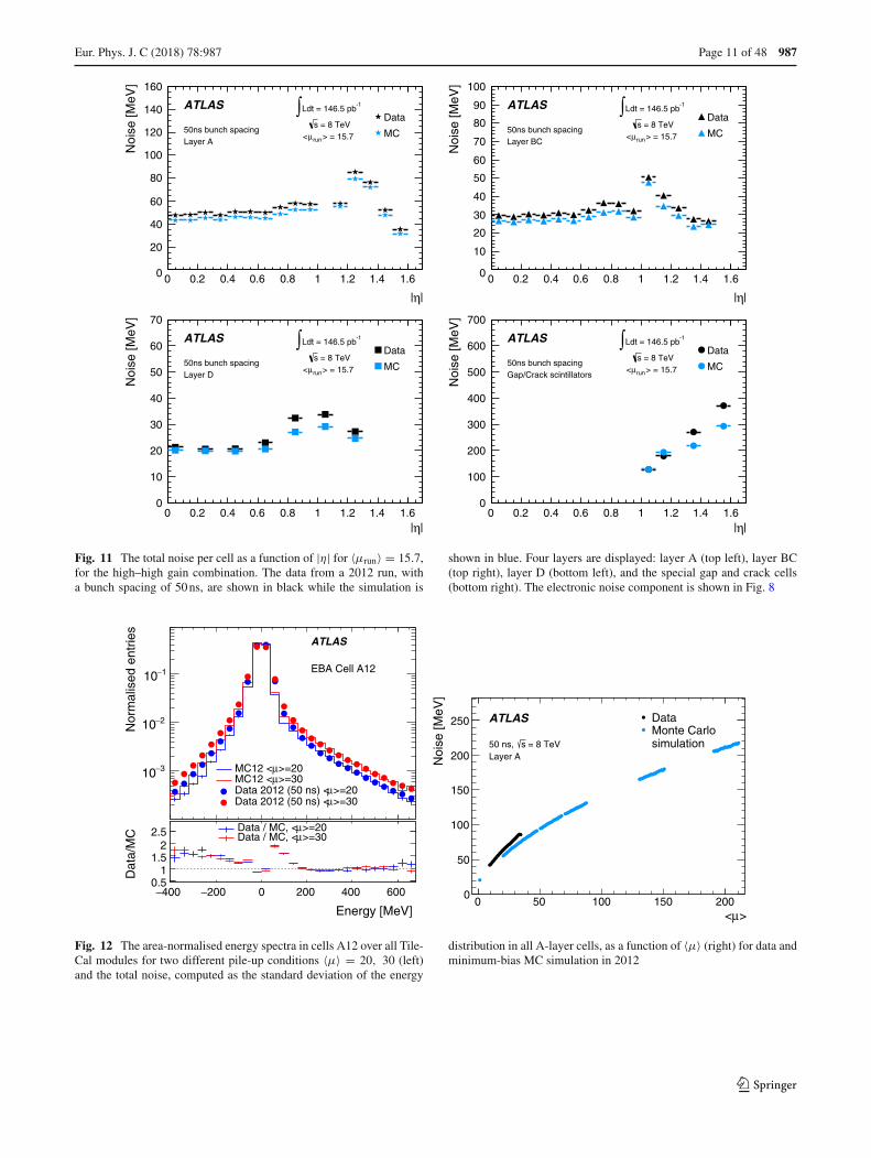
The total noise (electronic noise and contribution frompile-up) in different radial layers as a function of |η| fora medium pile-up run (average number of interactions perbunch crossing over the whole run 〈μrun〉 = 15.7) takenin 2012 is shown in Fig. 11. The plots make use of the η

symmetry of the detector and use cells from both η sides inthe calculation. In the EB standard cells (all except E-cells),where the electronic noise is almost flat (see Fig. 8), theamount of upstream material as a function of |η| increases [1],causing the contribution of pile-up to the total noise to vis-ibly decrease. The special cells (E1–E4), representing thegap and crack scintillators, experience the highest particleflux, and have the highest amount of pile-up noise, withcell E4 (|η| = 1.55) exhibiting about 380 MeV of noise at〈μrun〉 = 15.7 (of which about 5 MeV is attributed to elec-tronic noise). In general, the trends seen in the data for alllayers as a function of |η| are reproduced by the MC simu-lation. The total noise observed in data exceeds that in thesimulation, the differences are up to 20%.

The energy spectrum in the cell A12 is shown inFig. 12(left) for two different pile-up conditions with 〈μ〉 =20 and 〈μ〉 = 30. The mean energy reconstructed in Tile-Cal cells is centred around zero in minimum-bias events.

123


|η|

Noi

se [M

eV]

0

20

40

60

80

100

120

140

160

Data

MC

ATLAS

50ns bunch spacingLayer A

-1Ldt = 146.5 pb∫

= 8 TeVs

run> = 15.7μ<

|η|0 0.2 0.4 0.6 0.8 1 1.2 1.4 1.6 0 0.2 0.4 0.6 0.8 1 1.2 1.4 1.6

Noi

se [M

eV]

0

10

20

30

40

50

60

70

80

90

100

Data

MC

ATLAS

50ns bunch spacingLayer BC

-1Ldt = 146.5 pb∫

= 8 TeVs

run> = 15.7μ<

|η|

Noi

se [M

eV]

0

10

20

30

40

50

60

70

Data

MC

ATLAS

50ns bunch spacingLayer D

-1Ldt = 146.5 pb∫

= 8 TeVs

run> = 15.7μ<

|η|0 0.2 0.4 0.6 0.8 1 1.2 1.4 1.6 0 0.2 0.4 0.6 0.8 1 1.2 1.4 1.6

Noi

se [M

eV]

0

100

200

300

400

500

600

700

Data

MC

ATLAS

50ns bunch spacingGap/Crack scintillators

-1Ldt = 146.5 pb∫

= 8 TeVs

run> = 15.7μ<

Fig. 11 The total noise per cell as a function of |η| for 〈μrun〉 = 15.7,for the high–high gain combination. The data from a 2012 run, witha bunch spacing of 50 ns, are shown in black while the simulation is

shown in blue. Four layers are displayed: layer A (top left), layer BC(top right), layer D (bottom left), and the special gap and crack cells(bottom right). The electronic noise component is shown in Fig. 8

Nor

mal

ised

ent

ries

3−10

2−10

1−10

ATLAS

EBA Cell A12

>=20μMC12 <>=30μMC12 <

>=20μData 2012 (50 ns) <>=30μData 2012 (50 ns) <

Energy [MeV]

−400 −200 0 200 400 600

Dat

a/M

C

0.51

1.52

2.5 >=20μData / MC, <>=30μData / MC, <

>μ<0 50 100 150 200

Noi

se [M

eV]

0

50

100

150

200

250 ATLAS

= 8 TeVs50 ns, Layer A

DataMonte Carlosimulation

Fig. 12 The area-normalised energy spectra in cells A12 over all Tile-Cal modules for two different pile-up conditions 〈μ〉 = 20, 30 (left)and the total noise, computed as the standard deviation of the energy

distribution in all A-layer cells, as a function of 〈μ〉 (right) for data andminimum-bias MC simulation in 2012

123


137Cs source

CalorimeterTiles

PhotomultiplierTubes

IntegratorRead-out

(Cs & Particles)

Charge injection (CIS)

Digital Read-out(Laser & Particles)

Particles

Laser light

Fig. 13 The signal paths for each of the three calibration systems used by the TileCal. The physics signal is denoted by the thick solid line and thepath taken by each of the calibration systems is shown with dashed lines

Increasing pile-up widens the energy distribution both in dataand MC simulation. Reasonable agreement between data andsimulation is found above approximately 200 MeV. However,below this energy, the simulated energy distribution is nar-rower than in data. This results in lower total noise in sim-ulation compared with that in experimental data as alreadyshown in Fig. 11. Figure 12(right) displays the average noisefor all cells in the A-layer as a function of 〈μ〉. Since thislayer is the closest to the beam pipe among LB and EB lay-ers, it exhibits the largest increase in noise with increasing〈μ〉. When extrapolating 〈μ〉 to zero, the noise values areconsistent with the electronic noise.

4 Calibration systems

Three calibration systems are used to maintain a time-independent electromagnetic (EM) energy scale6 in the Tile-Cal, and account for changes in the hardware and electronicsdue to irradiation, ageing, and faults. The caesium (Cs) sys-tem calibrates the scintillator cells and PMTs but not thefront-end electronics used for collision data. The laser cali-bration system monitors both the PMT and the same front-end electronics used for physics. Finally, the charge injectionsystem (CIS) calibrates and monitors the front-end electron-ics. Figure 13 shows a flow diagram that summarises thecomponents of the read-out tested by the different calibra-tion systems. These three complementary calibration systemsalso aid in identifying the source of problematic channels.Problems originating strictly in the read-out electronics areseen by both laser and CIS, while problems related solely tothe PMT are not detected by the charge injection system.

The signal amplitude A is reconstructed in units of ADCcounts using the OF algorithm defined in Eq. (1). The con-

6 The corresponding calibration constant converts the calorimeter sig-nals, measured as electric charge in pC, to energy deposited by electronsthat would produce these signals.

version to channel energy, Echannel, is performed with thefollowing formula:

Echannel = A · CCs · Claser · CADC→pC,CIS/CTB (2)

where each Ci represents a calibration constant or correctionfactor, which are described in the following paragraphs.

The overall EM scale CTB was determined in dedicatedbeam tests with electrons incident on 11% of the productionmodules [6,27]. It amounts to 1.050 ± 0.003 pC/GeV with anRMS spread of (2.4 ± 0.1)% in layer A, with additional cor-rections applied to the other layers as described in Sect. 4.1.The remaining calibration constants in Eq. (2) are used tocorrect for both inherent differences and time-varying opticaland electrical read-out differences between individual chan-nels. They are calculated using three dedicated calibrationsystems (caesium, laser, charge injection) that are describedin more detail in the following subsections. Each calibrationsystem determines their respective constants to a precisionbetter than 1%.

4.1 Caesium calibration

The TileCal exploits a radioactive 137Cs source to maintainthe global EM scale and to monitor the optical and electricalresponse of each PMT in the ATLAS environment [30]. Ahydraulic system moves this Cs source through the calorime-ter using a network of stainless steel tubes inserted into smallholes in each tile scintillator.7 The beta decay of the 137Cssource produces 0.665 MeV photons at a rate of ∼ 106 Hz,generating scintillation light in each tile.8 In order to collect asufficient signal, the electrical read-out of the Cs calibration

7 The E3 and E4 cells are not part of this Cs mechanical system, andtherefore are not calibrated using the Cs source.8 Although the Cs signal can be measured from each single tile [5],the total Cs signal averaged over all tiles associated to the given cell isconsidered for the Cs constant evaluation.

123


Date [month and year]

Cae

sium

res

pons

e [a

.u.]

0.92

0.94

0.96

0.98

1

1.02

1.04

1.06

Layer A

Layer BC

Layer D

ATLAS

Jul 09 Jan 10 Jul 10 Jan 11 Jul 11 Jan 12 Jul 12 Dec 12 Jul 09 Jan 10 Jul 10 Jan 11 Jul 11 Jan 12 Jul 12 Dec 12

Date [month and year]

0

1

2

3

4

5

6

Dev

iatio

n fr

om e

xpec

ted

Cs

resp

onse

[%]

Layer A

Layer BC

Layer D

ATLAS

Fig. 14 The plot on the left shows the average response (in arbitraryunits, a.u.) from all cells within a given layer to the 137Cs source as afunction of time from July 2009 to December 2012. The solid line rep-resents the expected response, where the Cs source activity decreasesin time by −2.3%/year. The coloured band shows the declared preci-sion of the Cs calibration (± 0.3%). The plot on the right shows thepercentage difference of the response from the expectation as a func-

tion of time averaged over all cells in all partitions. Both plots displayonly the measurements performed with the magnetic field at its nominalvalue. The first points in the plot on the right deviate from zero, as theinitial HV equalisation was done in June 2009 using Cs calibration datataken without the magnetic field (not shown in the plot). The increasingCs response in the last three measurements corresponds to the periodwithout collisions after the Run 1 data-taking finished

is performed using the integrator read-out path; therefore theresponse is a measure of the integrated current in a PMT. As isdescribed in Sect. 4.3, dedicated calibration runs of the inte-grator system show that the stability of individual channelswas better than 0.05% throughout Run 1.

In June 2009 the high voltage (HV) of each PMT wasmodified so that the Cs source response in the same PMTswas equal to that observed in the test beam. Corrections areapplied to account for differences between these two envi-ronments, namely the activity of the different sources andhalf-life of 137Cs.

Three Cs sources are used to calibrate the three physicalTileCal partitions in the ATLAS detector, one in the LB andone in each EB. A fourth source was used for beam tests andanother is used in a surface research laboratory at CERN. Theresponse to each of the five sources was measured in April2009 [6] and again in March 2013 at the end of Run 1 usinga test module for both the LB and EB. The relative responseto each source measured on these two dates agrees to within0.2% and confirms the expected 137Cs activity during Run 1.

A full Cs calibration scan through all tiles takes approxi-mately six hours and was performed roughly once per monthduring Run 1. The precision of the Cs calibration in one typi-cal cell is approximately 0.3%. For cells on the extreme sidesof a partition the precision is 0.5% due to larger uncertaintiesassociated with the source position. Similarly, the precisionfor the narrow C10 and D4 ITC cells is 3% and ∼1%, respec-tively, due to the absence of an iron end-plate between thetile and Cs pipe. It makes more challenging the distinctionbetween the desired response when the Cs source is inside

that particular tile of interest versus a signal detected whenthe source moves towards a neighbouring tile row.

The Cs response as a function of time is shown inFig. 14(left) averaged over all cells of a given radial layer.The solid line, enveloped by an uncertainty band, representsthe expected response due to the reduced activity of the threeCs sources in the ATLAS detector (−2.3%/year). The errorbars on each point represent the RMS spread of the responsein all cells within a layer. There is a clear deviation fromthis expectation line, with the relative difference between themeasured and expected values shown in Fig. 14(right). Theaverage up-drift of the response relative to the expectationwas about 0.8%/year in 2009–2010. From 2010 when theLHC began operation, the upward and downward trends arecorrelated with beam conditions–the downward trends cor-respond to the presence of colliding beams, while the upwardtrends are evident in the absence of collisions. This effect ispronounced in the innermost layer A, while for layer D thereis negligible change in response. This effect is even more evi-dent when looking at pseudorapidity-dependent responsesin individual layers. While in most LB-A cells a deviationof approximately 2.0% is seen (March 2012 to December2012), in EB-A cells the deviation ranges from 3.5% (cellA13) to 0% (outermost cell A16). These results indicate thetotal effect, as seen by the Cs system, is due to the scintilla-tor irradiation and PMT gain changes (see Sect. 4.5 for moredetails).

The Cs calibration constants are derived using Cs calibra-tion data taken with the full ATLAS magnetic field system on,as in the nominal physics configuration. The magnetic field

123


0.0 0.1 0.2 0.3 0.4 0.5 0.6 0.7 0.8 0.9 1.0 1.1

1.2

1.3

1.4

1.6

eta

-1.04A1

-1.01A2

-1.09A3

-1.17A4

-1.16A5

-1.20A6

-1.04A7

-1.11A8

-1.15A9

-1.27A10

-.44B1

-.49B2

-.50B3

-.63B4

-.61B5

-.48B6

-.51B7

-.84B8

-.72B9

-.44C1

-.49C2

-.50C3

-.63C4

-.61C5

-.48C6

-.51C7

-.84C8

D0-.03

D1+.11

D2-.26

D3-.26

-.60A12

-.87A13

-.78A14

-.46A15

-.34A16

-.46B11

-.33B12 B13

+.21B14-.03

B15-.03

-.35C10

D4-.26

D5+.11

D6+.17

-.79E1

-1.17E2

-1.81E3

-2.64E4

<-2.0% -1.0% 0% 1.0% >2.0%

run 201625 2012-04-21 10:45:18

ATLAS

PMT gain variation (%)

Fig. 15 The mean gain variation in the PMTs for each cell type aver-aged over φ between a stand-alone laser calibration run taken on 21April 2012 and a laser run taken before the collisions on 19 March2012. For each cell type, the gain variation was defined as the mean of

a Gaussian fit to the gain variations in the channels associated with thiscell type. A total of 64 modules in φ were used for each cell type, withthe exclusion of known pathological channels

effectively increases the light yield in scintillators approxi-mately by 0.7% in the LB and 0.3% in the EB.

Since the response to the Cs source varies across thesurface of each tile, additional layer-dependent weights areapplied to maintain the EM scale across the entire calorime-ter [27]. These weights reflect the different radial tile sizesin individual layers and the fact that the Cs source passesthrough tiles at their outer edge.

The total systematic uncertainty in applying the EM scalefrom the test beam environment to ATLAS was found to be0.7%, with the largest contributions from variations in theresponse to the Cs sources in the presence of a magneticfield (0.5%) and the layer weights (0.3%) [27].

4.2 Laser calibration

A laser calibration system is used to monitor and correct forPMT response variations between Cs scans and to monitorchannel timing during periods of collision data-taking [31,32].

This laser calibration system consists of a single lasersource, located off detector, able to produce short light pulsesthat are simultaneously distributed by optical fibres to all9852 PMTs. The intrinsic stability of the laser light was foundto be 2%, so to measure the PMT gain variations to a precisionof better than 0.5% using the laser source, the response of thePMTs is normalised to the signal measured by a dedicatedphotodiode. The stability of this photodiode is monitored byan α-source and, throughout 2012, its stability was shown

to be 0.1%, and the linearity of the associated electronicsresponse within 0.2%.

The calibration constants, Claser in Eq. (2), are calculatedfor each channel relative to a reference run taken just aftera Cs scan, after new Cs calibration constants are extractedand applied. Laser calibration runs are taken for both gainsapproximately twice per week.

For the E3 and E4 cells, where the Cs calibration is notpossible, the reference run is taken as the first laser run beforedata-taking of the respective year. A sample of the mean gainvariation in the PMTs for each cell type averaged over φ

between 19 March 2012 (before the start of collisions) and21 April 2012 is shown in Fig. 15. The observed down-driftof approximately 1% mostly affects cells at the inner radiuswith higher current draws.

The laser calibration constants were not used during 2010.For data taken in 2011 and 2012 these constants were cal-culated and applied for channels with PMT gain variationslarger than 1.5% (2%) in the LB (EB) as determined by thelow-gain calibration run, with a consistent drift as measuredin the equivalent high-gain run. In 2012 up to 5% of thechannels were corrected using the laser calibration system.The laser calibration constants for E3 and E4 cells wereapplied starting in the summer of 2012, and were retroac-tively applied after the ATLAS data were reprocessed withupdated detector conditions. The total statistical and system-atic errors of the laser calibration constants are 0.4% for theLB and 0.6% for the EBs, where the EBs experience largercurrent draws due to higher exposure.

123


Fig. 16 Stability of the charge injection system constants for the low-gain ADCs (left) and high-gain ADCs (right) as a function of time in2012. Values for the average over all channels and for one typical chan-

nel with the 0.7% systematic uncertainty are shown. Only good channelsnot suffering from damaged components relevant to the charge injectioncalibration are included in this figure

4.3 Charge injection calibration

The charge injection system is used to calculate the constantCADC→pC,CIS in Eq. (2) and applied for physics signals andlaser calibration data. A part of this system is also used tocalibrate the gain conversion constant for the slow integratorread-out.

All 19704 ADC channels in the fast front-end electronicsare calibrated by injecting a known charge from the 3-in-1cards, repeated for a wide range of charge values (approxi-mately 0–800 pC in low-gain and 0–12 pC in high-gain). Alinear fit to the mean reconstructed signal (in ADC counts)yields the constantCADC→pC,CIS. During Run 1 the precisionof the system was better than 0.7% for each ADC channel.

Charge injection calibration data are typically taken twiceper week in the absence of colliding beams. For channelswhere the calibration constant varies by more than 1.0%the constant is updated for the energy reconstruction. Fig-ure 16 shows the stability of the charge injection constantsas a function of time in 2012 for the high-gain and low-gain ADC channels. Similar stability was seen throughout2010 and 2011. At the end of Run 1 approximately 1% ofall ADC channels were unable to be calibrated using the CISmostly due to hardware problems evolving in time, so defaultCADC→pC,CIS constants are used in such channels.

The slow integrator read-out is used to measure the PMTcurrent over ∼10 ms. Dedicated runs are periodically taken tocalculate the integrator gain conversion constant for each ofthe six gain settings, by fitting the linear relationship betweenthe injected current and measured voltage response. The sta-bility of individual channels is better than 0.05%, the averagestability is better than 0.01%.

4.4 Minimum-bias currents

Minimum-bias (MB) inelastic proton–proton interactions atthe LHC produce signals in all PMTs, which are used tomonitor the variations of the calorimeter response over timeusing the integrator read-out (as used by the Cs calibrationsystem).9 The MB rate is proportional to the instantaneousluminosity, and produces signals in all subdetectors, whichare uniformly distributed around the interaction point. In theintegrator circuit of the Tile Calorimeter this signal is seen asan increased PMT current I calculated from the ADC voltagemeasurement as:

I [nA] = ADC [mV] − ped [mV]Int. gain [M ] ,

where the integrator gain constant (Int. gain) is calculatedusing the CIS calibration, and the pedestal (ped) from physicsruns before collisions but with circulating beams (to accountfor beam background sources such as beam halo and beam–gas interactions). Studies found the integrator has a linearresponse (non-linearity < 1%) for instantaneous luminosi-ties between 1 × 1030 and 3 × 1034 cm−2s−1.

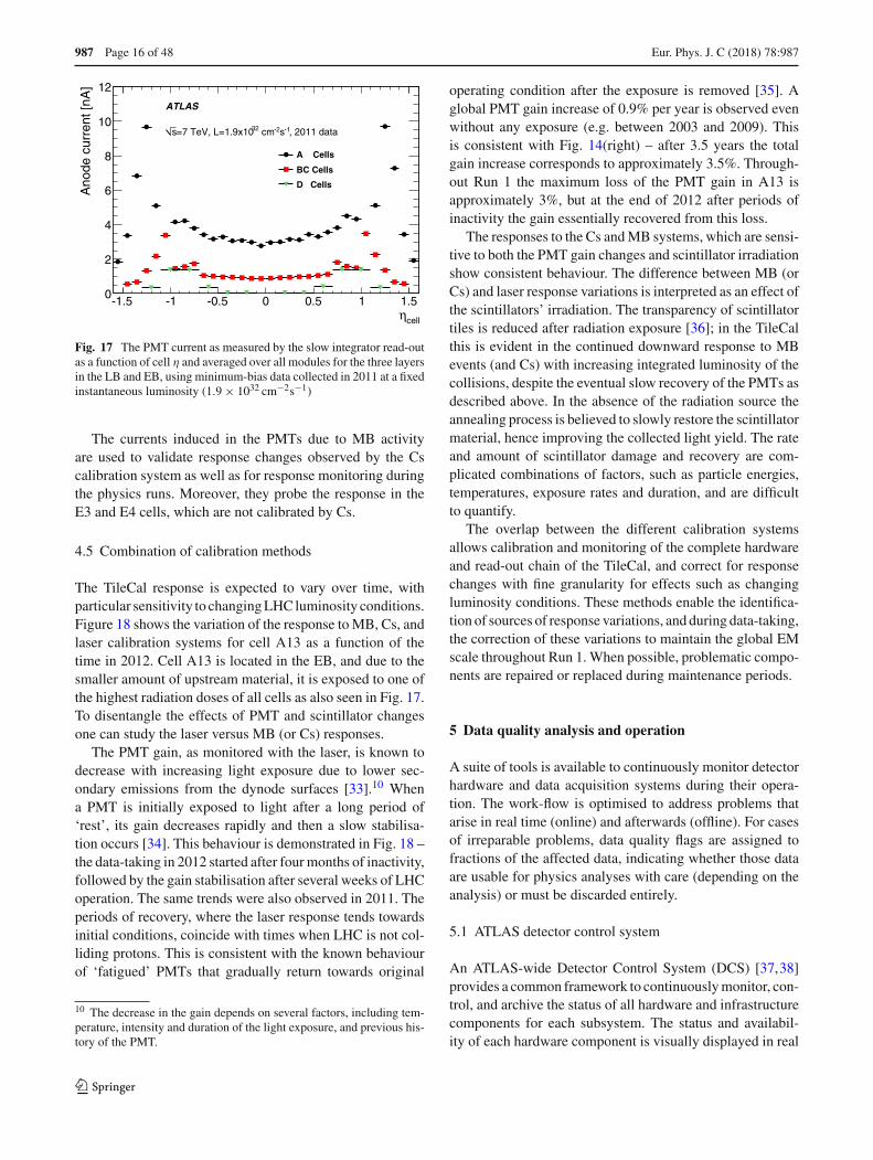
Due to the distribution of upstream material and the dis-tance of cells from the interaction point the MB signal seenin the TileCal is not expected to be uniform. Figure 17 showsthe measured PMT current versus cell η (averaged over allmodules) for a fixed instantaneous luminosity. As expected,the largest signal is seen for the A-layer cells which are closerto the interaction point, with cell A13 (|η| = 1.3) located inthe EB and (with minimal upstream material) exhibiting thehighest currents.

9 The usage of the integrators allows for a high rate of minimum-biasevents, much higher than could be achieved with the fast read-out.

123


cellη-1.5 -1 -0.5 0 0.5 1 1.5

Ano

de c

urre

nt [n

A]

0

2

4

6

8

10

12

A Cells

BC Cells

D Cells

ATLAS

, 2011 data-1s-2 cm32=7 TeV, L=1.9x10s

Fig. 17 The PMT current as measured by the slow integrator read-outas a function of cell η and averaged over all modules for the three layersin the LB and EB, using minimum-bias data collected in 2011 at a fixedinstantaneous luminosity (1.9 × 1032 cm−2s−1)

The currents induced in the PMTs due to MB activityare used to validate response changes observed by the Cscalibration system as well as for response monitoring duringthe physics runs. Moreover, they probe the response in theE3 and E4 cells, which are not calibrated by Cs.

4.5 Combination of calibration methods

The TileCal response is expected to vary over time, withparticular sensitivity to changing LHC luminosity conditions.Figure 18 shows the variation of the response to MB, Cs, andlaser calibration systems for cell A13 as a function of thetime in 2012. Cell A13 is located in the EB, and due to thesmaller amount of upstream material, it is exposed to one ofthe highest radiation doses of all cells as also seen in Fig. 17.To disentangle the effects of PMT and scintillator changesone can study the laser versus MB (or Cs) responses.

The PMT gain, as monitored with the laser, is known todecrease with increasing light exposure due to lower sec-ondary emissions from the dynode surfaces [33].10 Whena PMT is initially exposed to light after a long period of‘rest’, its gain decreases rapidly and then a slow stabilisa-tion occurs [34]. This behaviour is demonstrated in Fig. 18 –the data-taking in 2012 started after four months of inactivity,followed by the gain stabilisation after several weeks of LHCoperation. The same trends were also observed in 2011. Theperiods of recovery, where the laser response tends towardsinitial conditions, coincide with times when LHC is not col-liding protons. This is consistent with the known behaviourof ‘fatigued’ PMTs that gradually return towards original

10 The decrease in the gain depends on several factors, including tem-perature, intensity and duration of the light exposure, and previous his-tory of the PMT.

operating condition after the exposure is removed [35]. Aglobal PMT gain increase of 0.9% per year is observed evenwithout any exposure (e.g. between 2003 and 2009). Thisis consistent with Fig. 14(right) – after 3.5 years the totalgain increase corresponds to approximately 3.5%. Through-out Run 1 the maximum loss of the PMT gain in A13 isapproximately 3%, but at the end of 2012 after periods ofinactivity the gain essentially recovered from this loss.

The responses to the Cs and MB systems, which are sensi-tive to both the PMT gain changes and scintillator irradiationshow consistent behaviour. The difference between MB (orCs) and laser response variations is interpreted as an effect ofthe scintillators’ irradiation. The transparency of scintillatortiles is reduced after radiation exposure [36]; in the TileCalthis is evident in the continued downward response to MBevents (and Cs) with increasing integrated luminosity of thecollisions, despite the eventual slow recovery of the PMTs asdescribed above. In the absence of the radiation source theannealing process is believed to slowly restore the scintillatormaterial, hence improving the collected light yield. The rateand amount of scintillator damage and recovery are com-plicated combinations of factors, such as particle energies,temperatures, exposure rates and duration, and are difficultto quantify.

The overlap between the different calibration systemsallows calibration and monitoring of the complete hardwareand read-out chain of the TileCal, and correct for responsechanges with fine granularity for effects such as changingluminosity conditions. These methods enable the identifica-tion of sources of response variations, and during data-taking,the correction of these variations to maintain the global EMscale throughout Run 1. When possible, problematic compo-nents are repaired or replaced during maintenance periods.

5 Data quality analysis and operation

A suite of tools is available to continuously monitor detectorhardware and data acquisition systems during their opera-tion. The work-flow is optimised to address problems thatarise in real time (online) and afterwards (offline). For casesof irreparable problems, data quality flags are assigned tofractions of the affected data, indicating whether those dataare usable for physics analyses with care (depending on theanalysis) or must be discarded entirely.

5.1 ATLAS detector control system

An ATLAS-wide Detector Control System (DCS) [37,38]provides a common framework to continuously monitor, con-trol, and archive the status of all hardware and infrastructurecomponents for each subsystem. The status and availabil-ity of each hardware component is visually displayed in real

123


Time [dd/mm and year]

201202/03

201202/05

201201/07

201231/08

201231/10

Cel

l A13

res

pons

e va

riatio

n [%

]

−6

−5

−4

−3

−2

−1

0

1

2

]-1

To

tal I

nte

gra

ted

Del

iver

ed L

um

ino

sity

[fb

0

2

4

6

8

10

12

14

16

18

20

22

EB Cells A13

Minimum-bias integrator

Caesium

Laser

ATLAS = 8 TeVs2012 Data -1Total Delivered: 23.3 fb

Fig. 18 The change of response seen in cell A13 by the minimum-bias,caesium, and laser systems throughout 2012. Minimum-bias data coverthe period from the beginning of April to the beginning of December2012. The Cs and laser results cover the period from mid-March tomid-December. The variation versus time for the response of the threesystems was normalised to the first Cs scan (mid-March, before the startof collisions data-taking). The integrated luminosity is the total deliv-

ered during the proton–proton collision period of 2012. The down-driftsof the PMT gains (seen by the laser system) coincide with the collisionperiods, while up-drifts are observed during machine development peri-ods. The drop in the response variation during the data-taking periodstends to decrease as the exposure of the PMTs increases. The varia-tions observed by the minimum-bias and Cs systems are similar, bothmeasurements being sensitive to PMT drift and scintillator irradiation

time on a web interface. This web interface also provides adetailed history of conditions over time to enable trackingof the stability. The DCS infrastructure stores informationabout individual device properties in databases.

The TileCal DCS is responsible for tracking the low volt-age, high voltage, front-end electronics cooling systems, andback-end crates. The DCS monitoring data are used by auto-matic scripts to generate alarms if the actual values are out-side the expected operating conditions. Actions to addressalarm states can be taken manually by experts, or subject tocertain criteria the DCS system can automatically executeactions.

The TileCal DCS system monitors the temperature of thefront-end electronics with seven probes at various locationsin the super-drawer. A temperature variation of 1 ◦C wouldinduce a PMT gain variation of 0.2% [6]. Analyses done overseveral data periods within Run 1 indicated the temperatureis maintained within 0.2 ◦C.

One key parameter monitored by the Tile DCS is the HVapplied to each PMT; typical values are 650–700 V. Since theHV changes alter the PMT gain, an update of the calibrationconstants is required to account for the response change. Therelative PMT gain variation �G between a reference time trand a time of interest t depends on the HV variation over thesame period according to:

�G

G= HVβ(t)

HVβ(tr)− 1 (3)

where the parameter β is extracted experimentally for eachPMT. Its mean value is β = 7.0 with an RMS of 0.2 across97% of the measured PMTs; hence a variation of 1 V corre-sponds to a gain variation of 1% (for β = 7).

The TileCal high-voltage system is based on remote HVbulk power supplies providing a single high voltage to eachsuper-drawer. Each drawer is equipped with a regulator sys-tem (HVopto card) that provides fine adjustment of the volt-age for each PMT. One controller (HVmicro card) managestwo HVopto cards of the super-drawer. The HVmicro cardreports actual HV values to the DCS through a CANbus net-work every few seconds.

Several studies were performed to quantify the stabil-ity of the HV of the PMTs and to identify unstable PMTs.One study compares the value of the measured HV with theexpected HV for each PMT over the 2012 period. The differ-ence between the measured and set high voltage (�HV) foreach PMT is fitted with a Gaussian distribution, and the meanvalue is plotted for all good channels in a given partition.Good channels are all channels except those in modules thatwere turned off or in the so-called emergency state (describedlater). For each partition the mean value is approximately0 V with an RMS spread of 0.44 V, showing good agreement.Another study investigates the time evolution of �HV for agiven partition. The variation of the mean values versus timeis lower than 0.05 V, demonstrating the stability of the HVsystem over the full period of the 2012 collision run.

123


Date

Feb 12 Apr 12 Jun 12 Aug 12 Oct 12 Dec 12

G [%

]Δ

-20

-10

0

10

20

30

40

Laser Low GainGain extrapolated from HVCaesium

ATLAS

EBC64 PMT30

Fig. 19 One PMT of the EBC64 module with the largest gain varia-tion. This plot presents a comparison between the gain expected from theHV instability (tiny dots), the one measured by the laser (open squares)and Cs (full circles) systems during the whole 2012 run. One HV pointrepresents the averaged gain variation over one hour. The vertical struc-tures are due to power cycles. There is very good agreement betweenthe three methods, meaning that even large variations can be detectedand handled by the TileCal monitoring and calibration systems

In order to identify PMTs with unstable HV over time,�HV is computed every hour over the course of one day foreach PMT. Plots showing the daily variation in HV over peri-ods of several months are made. PMTs with �HV > 0.5 Vare classified as unstable. The gain variation for these unsta-ble channels is calculated using Eq. (3) (with knowledge ofthe β value for that particular PMT), and compared with thegain variation as seen by the laser and Cs calibration systems.These calibration systems are insensitive to electrical failuresassociated with reading back the measured HV and providea cross-check of apparent instabilities. Figure 19 shows thegain variation for one PMT that suffered from large instabili-ties in 2012, as measured by the HV and calibration systems.The gain variations agree between the three methods used.Only those channels that demonstrate instabilities in both theHV and calibration systems are classified as unstable. During2012, a total of only 15 PMTs (0.15% of the total number ofPMTs) were found to be unstable.

5.2 Online data quality assessment and monitoring

During periods of physics collisions, the Tile Calorimeterhas experts in the ATLAS control room 24 hours per dayand a handful of remote experts available on call to assist inadvanced interventions. The primary goal is to quickly iden-tify and possibly correct any problem that cannot be fixedlater in software, and that can result in overall data loss. TheATLAS data quality framework is designed to perform auto-matic checks of the data and to alert experts to potentialproblems that warrant further investigation [39].

Common problems identified by TileCal experts duringthe online shifts include hardware failures that do not auto-

matically recover, or software configuration problems thatmight present themselves as data corruption flags from theROD data integrity checks. The trigger efficiency and dataacquisition, as well as higher-level reconstruction data qual-ity, might be influenced by such problems.

5.3 Offline data quality review

Shortly after the data are taken, a small fraction is quicklyreconstructed using the Tier-0 computing farm within theATLAS Athena software framework [40]. Reconstructeddata are then used by the offline data quality experts withmore complex tools to evaluate the quality of the data. Theexperts are given 48 hours to identify, and, where possible, tocorrect problems, before the bulk reconstruction of the entirerun is made. The TileCal offline experts can update the con-ditions database, where information such as the calibrationconstants and status of each channel is stored. Channels thatsuffer from high levels of noise have calibration constantsin the database updated accordingly. For channels that sufferfrom intermittent data corruption problems, data quality flagsare assigned to the affected data to exclude the channels in thefull reconstruction during that period. This 48-hour period isalso used to identify cases of digitiser timing jumps and toadd the additional time phases to the time constants of thedigitiser affected to account for the magnitude of the timejump.

Luminosity blocks can be flagged as defective to iden-tify periods of time when the TileCal is not operating in itsnominal configuration. These defects can either be tolera-ble whereby corrections are applied but additional cautionshould be taken while analysing these data, or intolerablein which case the data are not deemed suitable for physicsanalyses. Defects are entered into the ATLAS Data Qual-ity Defect database [41] with the information propagating toanalyses as well as to integrated luminosity calculations.

One luminosity block nominally spans one minute, andremoving all data within that time can accumulate to a sig-nificant data loss. For rare situations where only a singleevent is affected by the data corruption, an additional error-state flag is introduced into the reconstruction data. This flagis used to remove such events from the analysis.

Once all offline teams review the run, it is sent to theTier-0 computing farm for bulk reconstruction, where theentire run is reconstructed using the most up-to-date condi-tions database. Subsequently the data can be re-reconstructedwhen reconstruction algorithms are improved and/or the con-ditions database is further refined to improve the descriptionof the detector.11 These data reprocessing campaigns typi-cally occur several months after the data are taken.

11 An example is the correction of time constants due to timing jumpsdiscovered only from fully reconstructed physics data, see Sect. 3.1.

123


Table 2 Summary of total integrated luminosity delivered by the LHC,recorded by ATLAS and approved for physics analyses (the data qual-ity deemed as good simultaneously from all ATLAS subsystems). Thenumbers in the parentheses denote the fraction of the integrated lumi-

nosity relative to the entry on the previous line. The last row lists thefraction of the ATLAS recorded data approved as good quality by theTile Calorimeter system

Integrated luminosity 2010 2011 2012

LHC delivered 48.1 pb−1 5.5 fb−1 22.8 fb−1

ATLAS recorded 45.0 pb−1 (93.5%) 5.1 fb−1 (92.7%) 21.3 fb−1 (93.4%)

ATLAS analysis approved 45.0 pb−1 (100%) 4.6 fb−1 (90.2%) 20.3 fb−1 (95.3%)

Tile data quality efficiency 100% 99.2% 99.6%

Fig. 20 The sources and amounts of integrated luminosity lost due toTile Calorimeter data quality problems in 2012 as a function of time.The primary source of luminosity losses comes from the stop-less read-out link (ROL) removal in the extended barrels accounting for 45.2 pb−1

of this loss. Power cuts or trips of the 200V power supplies account for22.6 pb−1. The last 4.9 pb−1 of losses stem from Laser Calibration ROD(LASTROD) busy events. The loss of 31.3 pb−1 due to a −25 ns timingshift in EBC are recovered after the data are reprocessed with updatedtiming constants. Each bin in the plot represents about two weeks ofdata-taking

5.4 Overall Tile Calorimeter operation

Overall the TileCal operation was highly successful in Run 1,with an extremely high fraction of data acceptable for aphysics analysis. A summary of the total integrated luminos-ity delivered to ATLAS and approved for analysis is shownin Table 2, along with the fraction of data passing the TileCalorimeter data quality reviews.

In 2012, the total integrated luminosity lost after the firstbulk reconstruction of the data due to TileCal data-quality-related problems was 104 pb−1 out of 21.7 fb−1, and is sum-marised in Fig. 20 as a function of time for various categoriesof intolerable defects.12 The primary source of Tile lumi-

12 The integrated luminosity values, quoted in this section and used inFig. 20, are estimated during the data-taking and are preliminary. Thesevalues therefore slightly differ from the final numbers listed in Table 2,obtained with the most recent offline calibration.

nosity losses are cases when a read-out link (ROL), whichtransmits data from the ROD to the subsequent chain in thetrigger and data acquisition system, is removed from pro-cessing. It implies no data are received from the four cor-responding modules. ROLs are disabled in situations whenthey are flooding the trigger with data (malfunctioning con-figuration or difficulty processing data), putting the triggerinto a busy state where effectively no data can be read fromany part of the detector. Removing a ROL during a run isdone in a so-called stop-less recovery state, whereby the runis not stopped, as restarting a run can take several minutes.One role of the online experts is to identify these cases andto respond by correcting the source of the removal and re-enabling the ROL in the run. After a new run begins any ROLsthat were previously removed are re-included. Improvementsfor handling ROL removals include adding monitoring plotscounting the number of reconstructed Tile cells, where largedrops can indicate a ROL removal, and an automatic ROLrecovery procedure. With the automatic recovery in place, asingle ROL removal lasts less than 30 seconds, and losses dueto ROL removal dramatically dropped in the second half of2012. As the removal of a ROL affects four consecutive mod-ules, this defect is classified as intolerable, and it accountedfor 45.2 pb−1 of data loss in 2012.

Power cuts or trips of the HV bulk power supply sourcesaccounted for 22.6 pb−1 of lost integrated luminosity. Thelast 4.9 pb−1 of loss came from situations when the laser RODbecame busy.13 During 2012 this was improved by promptingthe online expert to disable the laser ROD.

An additional loss of 31.3 pb−1 was due to a 25 ns timingshift in a large fraction of the EBC partition which was notcaught by the online or offline experts or tools. Improvementsfor large timing shifts include data quality monitoring warn-ings when the reconstructed time for large numbers of Tilechannels differs from the expected value by a large amount.These data are subsequently recovered in later data repro-cessing campaigns when the timing database constants areupdated accordingly.

13 Laser events are recorded in parallel with physics data in emptybunch crossings.

123


Fig. 21 The percentage of theTileCal cells that are masked inthe reconstruction as a functionof time starting from June 2010.Periods of recovery correspondto times of hardwaremaintenance when the detectoris accessible due to breaks in theaccelerator schedule. Eachsuper-drawer LB (EB) failurecorresponds to 0.43% (0.35%)of masked cells. The totalnumber of cells (including gap,crack, and minimum-bias triggerscintillators) is 5198.Approximately 2.9% of cellswere masked in February 2013,at the end of the proton–leaddata-taking period closing theRun 1 physics programme Date [dd/mm/yy]

18/06/10 18/10/10 18/02/11 20/06/11 20/10/11 19/02/12 21/06/12 21/10/12 20/02/13

Fra

ctio

n of

mas

ked

cells

[%]

0

1

2

3

4

5 ATLAS

There are several operational problems with the LVPSsources that contribute to the list of tolerable defects. In somecases the LVPS fails entirely, implying an entire module isnot analysed. The failure rate was one LVPS per month in2011 and 0.5 LVPS per month in 2012. The faulty LVPSsources were replaced with spares during the maintenancecampaigns in the ATLAS cavern at the end of each year.

In addition to overall failures, sometimes there are prob-lems with the low voltage supplied to the HVopto card, whichmeans the PMT HV can be neither controlled nor measured.In this case the applied HV is set to the minimum value,putting the module in an emergency state. The calibrationand noise constants for all channels within a module in emer-gency mode are updated to reflect this non-nominal state.

Finally, the LVPS suffered from frequent trips correlatedwith the luminosity at a rate of 0.6 trips per 1 pb−1. Automaticrecovery of these modules was implemented, to recover thelost drawer. During the maintenance period between 2011and 2012, 40 new LVPS sources (version 7.5) with improveddesign [42] were installed on the detector. In 2012 there werea total of about 14,000 LVPS trips from all modules, only oneof which came from the new LVPS version. After the LHCRun 1, all LVPS sources were replaced with version 7.5.

Figure 21 shows the percentage of the TileCal cellsmasked in the reconstruction as a function of time. Thesecells are located in all areas of the detector, with no one areasuffering from a large number of failures. The main reasonsfor masking a cell are failures of LVPS sources, evident bythe steep steps in the figure. Other reasons are severe datacorruption problems or very large noise. The periods of main-tenance, when faulty hardware components are repaired orreplaced (when possible), are visible by the reduction of thenumber of faulty cells to near zero. For situations when cellenergy reconstruction is not possible the energy is interpo-lated from neighbouring cells. The interpolation is linear in

energy density (energy per cell volume) and is done indepen-dently in each layer, using all possible neighbours of the cell(i.e. up to a maximum of eight). In cases where only one oftwo channels defining a cell is masked the energy is taken tobe twice that of the functioning channel.

6 Performance studies

The response of each calorimeter channel is calibrated tothe EM scale using Eq. (2). The sum of the two channelresponses associated with the given read-out cell forms thecell energy, which represents a basic unit in the physics objectreconstruction procedures. Cells are combined into clusterswith the topological clustering algorithm [28] based on thesignificance of the absolute value of the reconstructed cellenergy relative to the noise, S = |E |/σ . The noise σ com-bines the electronic (see Sect. 3.2) and pile-up contributions(Sect. 3.3) in quadrature. Clusters are then used as inputs tojet reconstruction algorithms.

The ATLAS jet performance [43,44] and measurementof the missing transverse momentum [45] are documentedin detail in other papers. The performance studies reportedhere focus on validating the reconstruction and calibrationmethods, described in previous sections, using the isolatedmuons, hadrons and jets entering the Tile Calorimeter.

6.1 Energy response to single isolated muons

Muon energy loss in matter is a well-understood process [46],and can be used to probe the response of the Tile Calorime-ter. For high-energy muons, up to muon energies of a fewhundred GeV, the dominant energy loss process is ionisa-tion. Under these conditions the muon energy loss per unitdistance is approximately constant. This subsection studies

123


Table 3 Selection criteriaapplied to the event, track, andmuon used in the cosmic muonsanalysis. A description andmotivation of each cut can befound in the text

Cut Variable Requirement

1 Number of muon tracks Nμ Nμ = 1

2 Number of track hits in Pixel + SCT ≥ 8

3 Reconstructed track distance from origin |d0| ≤ 380 mm (transverse),

|z0| ≤ 800 mm (longitudinal)

4 Polar angle of track relative to vertical axis |θμ| > 0.13 rad

5 Muon momentum 10 GeV < pμ < 30 GeV

6 Muon path length through cell �x > 200 mm

7 Cell energy �E > 60 MeV

8 Track impact point at inner and outer radial point of cell |φc − φinner| < 0.04,

|φc − φouter| < 0.04

the response to isolated muons from cosmic-ray sources andto W → μν events from pp collisions.

Candidate muons are selected using the muon RPC andTGC triggering subsystems of the Muon Spectrometer. Amuon track measured by the Pixel and SCT detectors isextrapolated through the calorimeter volume, taking intoaccount the detector material and magnetic field [47]. A lin-ear interpolation is performed to determine the exact entryand exit points of the muon in every crossed cell to computethe distance traversed by the muon in a given TileCal cell.The distance (�x) together with the energy deposited in thecell (�E) are used to compute the muon energy loss per unitdistance, �E/�x .

The measured �E/�x distribution for a cell can bedescribed by a Landau function convolved with a Gaus-sian distribution, where the Landau part describes the actualenergy loss and the Gaussian part accounts for resolutioneffects. However, the fitted curves show a poor χ2 fit to thedata, due to high tails from rare energy loss mechanisms, suchas bremsstrahlung or energetic gamma rays. For this reasona truncated mean 〈�E/�x〉t is used to define the averagemuon response. For each cell the truncated mean is com-puted by removing a small fraction (1%) of entries with thehighest �E/�x values. The truncated mean exhibits a slightnon-linear scaling with the path length �x . This non-linearityand other residual non-uniformities, such as the differencesin momentum and incident angle spectra, are to a large extentreproduced by the MC simulation. To compensate for theseeffects, a double ratio formed by the ratio of the experimentaland simulated truncated means is defined for each calorime-ter cell as:

R ≡ 〈�E/�x〉datat

〈�E/�x〉MCt

. (4)

The double ratio R is used to estimate the calorimeterresponse as a function of various detector geometrical quan-tities (layer, φ, η, etc). Deviations of the double ratio from

unity may indicate poor EM energy scale calibration in theexperimental data.

6.1.1 Cosmic-ray muon data

Muons from cosmic-ray showers, called cosmic muons, areused as a cross-check of energy reconstruction and calibra-tion complementary to the collision data. At sea level, cosmicmuons can have energies up to a TeV or more, but most ofthe muons are at lower energies, with the mean energy beingapproximately 4 GeV [46].

Candidate cosmic muons are triggered during emptybunch crossings in physics runs in a dedicated data streamallocated for muon candidates identified by the muon spec-trometer trigger system if at least one track is matched tothe inner detector tracking system. In total there are approxi-mately one million such events triggered in each year studied(2008, 2009, 2010).

The energy in TileCal channels is reconstructed using theiterative OF method (see Sect. 3). The muon tracks, recon-structed using Pixel and SCT detectors with a dedicated algo-rithm, are extrapolated through the volume of the calorime-ter in both upward and downward directions. This allows tostudy the response of the TileCal modules in top and bottomparts of the detector.

The event selection criteria used to select events for thecosmic muons analysis are summarised in Table 3. A candi-date cosmic-muon event is required to have exactly one trackassociated with a reconstructed muon (Cut 1), with at leasteight hits in the Pixel plus SCT detectors (Cut 2). A cut onthe maximum distance of the reconstructed track from theorigin of the coordinate system in both the transverse (d0)and longitudinal (z0) components (Cut 3) is used to selectwell-reconstructed tracks that follow the projective geome-try of the calorimeter. Muons with a trajectory close to thevertical direction are poorly measured in the TileCal due tothe vertical orientation of the scintillating tiles, hence Cut 4is used to remove the very central cells located within the

123


[MeV/mm]xΔ/EΔ

Ent

ries

/ 0.1

MeV

/mm

0

100

200

300

400

500

600

700

800

900

Cosmic-ray data 2008MC

ATLAS

Long Barrel cell A3

[MeV/mm]xΔ/EΔ0.5 1 1.5 2 2.5 3 3.5 4 4.5 5 0.5 1 1.5 2 2.5 3 3.5 4 4.5 5

Ent

ries

/ 0.1

MeV

/mm

0

500

1000

1500

2000

2500

3000

Cosmic-ray data 2008MC

ATLAS

Long Barrel cell D2

Fig. 22 Distributions of the energy deposited by cosmic muons perunit of path length, �E/�x , in the two cells in the long barrel, A3(left) and D2 (right) obtained using 2008 experimental (full points) andsimulated (solid lines) data. The A3 (D2) cell in the long barrel covers

the region 0.2 < |η| < 0.3 (0.3 < |η| < 0.5) and is located in theinnermost (outermost) calorimeter layer. The function curve overlaidon top of the experimental data is a Landau distribution convolved witha Gaussian distribution

vertical coverage of the inner detector. The last two require-ments (Cut 3 and Cut 4) effectively remove muons at very lowpseudorapidities. The muon is required to have momentumin the range 10–30 GeV to minimise the effects of multiplescattering at low momentum, and to reduce radiative energylosses at higher momentum, which could produce large fluc-tuations in the results. The muon path length through a cellmust be larger than 200 mm. An energy of at least 60 MeV14

has to be released in that cell to remove contributions fromnoise. Cut 8 is used to reduce contributions from multiplescattering, such that the track’s azimuthal impact point at theinner (outer) radial point of the cell, φinner(φouter) is within0.04 radians of the cell centre φc coordinate (with a cell widthof �φ = 0.1).

The response to cosmic muons in the calorimeter is alsostudied using MC simulated data. The cosmic-muon energyand flux spectra as measured at sea-level [48] are used as inputinto the simulation. The material between the surface and theATLAS cavern is simulated, including the cavern volumesand detector access shafts. Air showers are not simulated buthave negligible impact due to the selection requirements forsingle-track events. The �E/�x distributions for the 2008cosmic-muon data and MC simulation are shown in Fig. 22for cells A3 (left) and D2 (right) in the long barrel. The A3(D2) cell covers the region 0.2 < |η| < 0.3 (0.3 < |η| < 0.5)and is located in the innermost (outermost) calorimeter layer.Differences between the experimental and simulated data arediscussed in the following paragraphs.

14 The value corresponds approximately to 3σ of the typical cell noisedistribution.

Verification of the radial layer intercalibrationThe calibration between cells within the same layer is investi-gated using the double ratio formed by the ratio of the exper-imental and simulated truncated means, as shown in Eq. (4).The typical non-uniformity of all cells in a given layer isfound to be approximately 2% for all layers every year. Thiscan be explained by the variations in the optical and electricalcomponents of the calorimeter.

Several sources of systematic uncertainty, summarised inTable 4, are considered in the studies of cosmic muons. Thesystematic variations 1–5 are related to the selection criteria.The results are assumed to be stable for different values usedin the selection criteria. This assumption is checked by vary-ing the values in the specified range and repeating the anal-ysis for every variation, both for data and MC simulations.The resulting differences contribute to the total systematicuncertainty. Differences in the response along the muon paththrough the detector and due to signal evaluation methodshould be well described by MC. Two systematic variations,applied both to data and MC, are introduced to verify thisassumption. Variation 6 compares the response in the upperpart of the detector (φc > 0), where these muons enter thedetector, and in the lower part (φc < 0), after the muons passthrough a large fraction of the detector. The uncertainty ofthe method used to evaluate the detector’s response to cos-mic muons is considered as source 7. Source 8 reflects thedifferent spread of the experimental and simulated �E/�xdistributions. The effect on the determination of the truncatedmean is estimated to be 0.3% using a toy MC simulation. Thefinal classes of uncertainties, 9 and 10, concern the signal

123


Table 4 Different sources of systematic uncertainty considered in theanalysis of the cosmic muons. Sources 1–5 are associated with theevent selection procedure, other sources are relevant for the double ratioresponses. The distributions of the parameters used in the analysis are

reported. In the case of source 3 for each track and each cell the valueof the maximal path length, MaxPath, is determined by the dimensionsof the cell

Source Systematic uncertainty Parameter distribution and variation

1 |θμ| (Cut 4 Table 3) Uniform [0.10, 0.15]

Uniform [5 GeV < pμ < 10 GeV,

2 pμ (Cut 5 Table 3) 10 GeV < pμ < 30 GeV,

30 GeV < pμ < 50 GeV]

3 �x (Cut 6 Table 3) Uniform [�xmin, �xmax]

with �xmin = MaxPath/2-100 mm

�xmax = �xmin + (MaxPath)/2

4 �E (Cut 7 Table 3) Uniform [30 MeV, 90 MeV]

5 |φc − φinner|, |φc − φouter| (Cut 8 Table 3) Uniform [0.03, 0.05]

6 φc Uniform φc > 0, φc < 0

7 �E/�x truncation Uniform 0%, 1%, 2%

8 Smearing of simulated �E/�x Gaussian μ = 0, σ = 0.3%

9 Uncertainty in radial calibration correction Gaussian μ = 0, σ = 0.3%

10 Uncertainty in up-drift and magnetic field effects Gaussian μ = 0, σ = 1.0% (LB), 0.6% (EB)

Table 5 Double ratio given in Eq. (4) by the ratio of the experimentaland simulated �E/�x truncated means for different layers in the longbarrel (LB) and extended barrel (EB), for the three data periods usingcosmic-muon data. The sources of uncertainty are described in the text.Larger uncertainties in the EB-A layer reflect that fewer cosmic muonssatisfy the selection criteria. A maximum difference of 4% is observedbetween the layer calibrations

R2008 R2009 R2010

LB-A 0.966 ± 0.012 0.972 ± 0.015 0.971 ± 0.011

LB-BC 0.976 ± 0.015 0.981 ± 0.019 0.981 ± 0.015

LB-D 1.005 ± 0.014 1.013 ± 0.014 1.010 ± 0.013

EB-A 0.964 ± 0.043 0.965 ± 0.032 0.996 ± 0.037

EB-B 0.977 ± 0.018 0.966 ± 0.016 0.988 ± 0.014

EB-D 0.986 ± 0.012 0.975 ± 0.012 0.982 ± 0.014

calibration procedures performed in the test beam and in situin ATLAS (already discussed in Sect. 4). The correspond-ing variations are only applied to the MC. The parametersof each source of systematic uncertainty are considered asrandom variables and their values are selected according tothe distributions reported in Table 4. In the case of sources3, 8 and 9 the errors are treated as uncorrelated and a differ-ent value is considered for each layer. To evaluate the totalsystematic uncertainty, 2500 working points are generated inthe parameter phase-space and for each of them the analy-sis is performed and the double ratio calculated. A Gaussiandistribution is observed for each layer and the standard devi-ation, σ , is taken as the associated systematic uncertainty.The contribution of statistical errors is negligible.

Table 5 shows the double ratio and its total uncertainty perlayer for all three years under study. These results can be used

to validate the calibration procedure including all correctionsas mentioned in Sect. 4. A method based on Bayes’ theoremis used to establish the uniformity of the layer response ineach year [49]. The probability function that the six mea-sured double ratios �R = (RLB−A, . . . , REB−D) correspondto layer responses �μ = (μLB−A, . . . , μEB−D) is proportionalto the likelihood L( �μ| �R), as uniform prior probabilities areassumed. Since the distribution of the double ratio is foundto be Gaussian in each layer, the likelihood is constructed assix-dimensional Gaussian function

L(μ|R) ∝ exp(−0.5 · ( �μ − �R)T V−1( �μ − �R)

)(5)

where V is the error matrix obtained from the analyses over2500 working points described above. For each pair of layersl, l ′, the posterior probability f (μl , μl ′ | �R) is evaluated byintegrating Eq. (5) over the remaining layers. It is found thatthe response of layer D in the long barrel differs from thatof layers A and BC by 4σ and 3σ , respectively, for all years(see Sect. 6.4 for more details). The response for all otherlayer pairs is found to be consistent. The total error in theEM energy scale for all cells in a fixed layer is found tobe approximately 2%, including uncertainties of the cosmicmuons analysis, uncertainties in the determination of the EMscale at test beams and subsequent application in ATLAS, andthe uncertainty in the simulation of the TileCal response tomuons.

A maximum-likelihood fit is used to estimate the meancalorimeter response (μy) over all layers for a given year(y), taking into account the uncertainties and correlations.The ratios μy/μy′ for y �= y′ and y, y′ ∈ {2008, 2009, 2010}

123


Table 6 Selection criteriaapplied to the events, tracks, andmuons for the collision muonanalysis

Cut Variable Requirement

1 Number of muon tracks Nμ Nμ = 1

2 Transverse mass mT mT > 40 GeV

3 Missing transverse momentum EmissT Emiss

T > 25 GeV

4 Polar angle of track relative to vertical axis |θμ| > 0.13 rad

5 Muon momentum 20 GeV < pμ < 80 GeV

6 Transverse momentum around track within �R < 0.4: pcone40T < 1 GeV

7 LAr calorimeter energy around track within �R < 0.4: ELAr < 3 GeV

8 Muon path length through cell �x > 100 mm

9 Cell energy �E > 60 MeV

are then computed, and are found to be consistent with unity.Within uncertainties the response of the calorimeter layersto cosmic-muon data is found to be stable, confirming thecalibration systems are able to follow the variations of thePMT gains and to compensate for the drift of response peryear to better than 1% in the long barrel and better than 3%in the extended barrel.

The double ratios listed in Table 5 are approximately 0.97,except for the LB-D layer, with a quoted uncertainty of theorder of 1.5%. Nevertheless, the differences from unity arewell within the TileCal EM scale uncertainty of 4% mea-sured in studies of isolated particles and in the beam tests [6].Detailed discussion and the comparison with the results ofthe isolated collision muons’ analysis (next section) are pre-sented in Sect. 6.4.

6.1.2 Isolated collision muons

The calorimeter performance is also assessed with isolatedmuons from W → μν processes originating in proton–proton collisions, complementary to the cosmic-muon stud-ies presented in previous subsection. Data from proton–proton collisions in 2010–2012 are analysed. Events werecollected using a L1 muon trigger which accepts events withsizeable muon pT originating from the interaction point. Atotal of approximately one billion events are selected for thesethree years. The event selection is further refined using thecriteria listed in Table 6. Cuts 1–3 are used to select W → μν

events and to suppress background from multi-jet processes.The transverse mass (mT), Cut 2, is defined as follows:

mT =√

2pμT E

missT (1 − cos[�φ(pμ

T ,pmissT )]),

where pμT is the vector of the muon’s transverse momen-

tum and pmissT stands for the vector of the missing transverse

momentum. The scalar variables denote the correspondingvector magnitude, pμ

T ≡ |pμT | and Emiss

T ≡ |pmissT |.

An explicit cut on missing transverse momentum is made(Cut 3) by requiring Emiss

T > 25 GeV in order to further

reduce background from jet production. Similar to the cos-mic muons analysis, a cut on the polar angle relative to thevertical axis is applied (Cut 4) and only muons in a lowmomentum range [20 GeV, 80 GeV] are selected (Cut 5). Thecontribution from nearby particles is suppressed by requir-ing the selected tracks to be well isolated within a cone ofsize �R = √

(�φ)2 + (�η)2 = 0.4 in the tracking detector(Cut 6) and the response in the upstream liquid argon (LAr)calorimeter must be compatible with a minimum-ionisingparticle (Cut 7). The muon path length through a cell isrequired to be larger than 100 mm (Cut 8), and the cell energyhas to be greater than 60 MeV to remove residual noise con-tributions (Cut 9).

The same selection criteria are applied to MC simulateddata. The W → μν events were generated using the leading-order generators Pythia 6 [23] in 2010, and Sherpa [50]in 2011 and 2012. The full ATLAS digitisation and recon-struction is performed on the simulated MC data. Unfortu-nately, data and MC events in 2010 were processed withdifferent reconstruction algorithms15 that in the end biasesthe data/MC ratio. Therefore, only the results from 2011 and2012 are reported here.

Cell response uniformityThe double ratios given in Eq. (4) by ratios of the truncatedmeans of the data and MC �E/�x distributions are usedto quantify the cell response uniformity in φ. The system-atic uncertainty associated with the non-uniformity in theresponse for cells of the same type in the considered φ sliceis quantified using a maximum-likelihood method. The like-lihood function with mean response μ and non-uniformity sis defined as follows:

L =Nc∏

c=1

1√2π · √

(σ 2c + s2)

exp

⎡

⎣−1

2

(Rc − μ√σ 2c + s2

)2⎤

⎦

(6)

15 Data in 2010 were reconstructed with iterative OF method, while inMC simulation the non-iterative approach was applied.

123


where the product runs over 64 modules in φ for each cellc of the same type. Here Rc is the double ratio from Eq. (4)and σc the statistical uncertainty for the cell under con-sideration. The maximum is effectively found by minimis-ing the unbinned log-likelihood −2 logL, varying the non-uniformity s.

The results of the fits are shown in Fig. 23 for the meanresponse μ (top) and non-uniformity in the azimuthal angles (bottom) in 2012. Cut 4 in Table 6 reduces the number ofmuons crossing the most central calorimeter cells, and thereare too few detected muons to include the cells with |η| < 0.1in the analysis. A similar study is done also for 2011 data.The mean double ratio across all cells is consistent with unity.Moreover, the double ratio is found to be constant across η

in each layer. Upper limits on the average non-uniformity inφ, quantified by the spread in response amongst calorimetercells of a given cell type, is found to be about 5% in both2011 and 2012 data.

The amount of energy deposited in a cell depends on thegeometrical properties, such as the amount of upstream deadmaterial and cell-specific calibration constants. In generalthere exists a symmetry between η > 0 and η < 0. As onegoes to increasing radius (layers A→BC→D), the valuesof the truncated means remain approximately the same. Asimilar trend is observed for the 2011 data.

Verification of the radial layer intercalibrationThe double ratio of the observed and simulated response iscalculated for each radial calorimeter layer for each data-taking year considered in the analysis. The systematic uncer-tainties associated with the event selection and the responseevaluation are listed in Table 7. These variations are consid-ered as random variables and their values selected accordingto uniform probability distributions. In total, 1000 combina-tions in the parameter phase-space are generated by vary-ing each of the applied cuts. The analysis is repeated foreach combination, similarly to the cosmic muons analysis(Sect. 6.1.1). The same method exploiting a six-dimensionalGaussian function is used and the mean response per layer isdetermined by maximum-likelihood fit for each data-takingyear (2011, 2012), taking into account the correlations of thesystematic uncertainties between the layers.

The double ratios together with the total uncertainties arereported in Table 8. The results indicate that the radial layersLB-A, LB-BC, EB-A, EB-B and EB-D were well intercali-brated in 2011 and 2012. It was found that the layer LB-Dhad higher response than the layers LB-A and LB-BC; thedifference of +3% is further discussed in Sect. 6.4.

Time stabilityThe double ratio defined in Eq. (4) as the ratio of theresponses in experimental and simulated data, averaged overall calorimeter cells of the same type, is calculated for allcell types for each year (2011, 2012). The selection cri-

teria associated with the systematic uncertainties reportedin Table 7 are varied and used to generate 1000 workingpoints. For each such point, the analysis is repeated. Simi-larly to the radial layer intercalibration studies, a model with atwo-dimensional (2011, 2012) Gaussian function is applied.The log-likelihood is minimised to fit the mean double ratioresponse for each year taking into account the correlationsbetween the years, also obtained from the varied analyses.The relative difference of the fitted responses between twoyears is computed as

�2011→2012 ≡ Rc2012 − Rc

2011

Rc2011

for each cell of a given type, to quantify the responsechange. The average difference across all cells is found tobe 〈�2011→2012〉 = (0.6 ± 0.1)%, indicating good stabilityof the response.16 The distribution of �2011→2012 over celltypes shows an RMS spread of 0.96%.

6.2 Energy response with hadrons

The calorimeter response can be also tested using singlehadrons and jets. Compared to muons, these objects depositmore energy in the hadronic calorimeter and therefore theresponse to higher energies can be probed. In addition, theMC simulations of objects interacting hadronically are com-pared with experimental data.

6.2.1 Single hadrons

The energy response of the TileCal is probed in situ by study-ing the ratio of a charged hadron’s energy (E), as measuredby the TileCal, to that of the hadron’s momentum (p), as mea-sured by the ATLAS inner detector system [1]. The energiesof hadrons in data and MC events are calibrated to the elec-tromagnetic energy scale. The data-to-MC double ratio givenby 〈E/p〉data/〈E/p〉MC should be approximately one, withdeviations from unity possibly due to poor EM scale calibra-tion in the data or differences in the MC description of themore complex hadron shower development (relative to themuon studies).

The datasets used in this analysis are based on the col-lision data taken at the LHC during 2010–2012. In 2010,92 nb−1 of data were collected using the Minimum BiasTrigger Scintillators (MBTS). In 2011 and 2012 the datawere triggered using fixed-rate random triggers, correspond-ing to effective integrated luminosities of 15.5 nb−1 and

16 The precision of the Cs system is approximately 0.3% as mentionedin Sect. 4.1. The steeper response up-drift observed in second half of2012 (see Fig. 14, right) might also contribute, since the Cs calibrationconstants were typically updated once per month.

123


Fig.23

Vis

ualis

atio

nof

the

Tile

Cal

inth

e(z

,r)

plan

esh

owin

gth

ere

sults

for

the

fitpa

ram

eter

sof

Eq.

(6)

for

(top

)th

em

ean

doub

lera

tiore

spon

seμ

and

(bot

tom

)th

eno

n-un

ifor

mity

inφ

ofth

edo

uble

ratio

s.Sh

own

for

allc

ells

with

|η|>

0.1,

usin

gth

e20

12da

taan

dM

Csi

mul

atio

n

123


Table 7 The variationsassociated with the eventselection procedure andresponse evaluation consideredas the sources of systematicuncertainty in the collisionmuon analysis. The distributionsof the parameters are reported

Source Systematic uncertainty Parameter distribution and variation

1 |θμ| (Cut 4 Table 6) Uniform [0.1238, 0.1365]

Uniform [20 GeV < pμ < 35 GeV,

2 pμ (Cut 5 Table 6) 35 GeV < pμ < 50 GeV,

50 GeV < pμ < 80 GeV]

3 �x (Cut 8 Table 6) Uniform [95 mm, 105 mm]

4 �E (Cut 9 Table 6) Uniform [30 MeV, 90 MeV]

5 Fraction of high tail excluded to compute truncated mean Uniform [0%, 1%, 2%]

Table 8 Double ratio given in Eq. (4) by the ratio of the experimentaland simulated �E/�x truncated means for different layers in the longbarrel (LB) and extended barrel (EB), using isolated muons from W →μν in data and MC events in 2011 and 2012. The sources of uncertaintyare described in the text

R2011 R2012

LB-A 0.996±0.006 1.003±0.006

LB-BC 1.001±0.004 1.005±0.005

LB-D 1.031±0.009 1.028±0.008

EB-A 1.007±0.013 1.025±0.008

EB-B 1.001±0.006 1.012±0.007

EB-D 1.008±0.010 1.012±0.010

Table 9 The selection criteria used for the E/p analysis with singleisolated hadrons

Cut Selection criteria

1 Track pT > 2 GeV

2 Extrapolated tracks |ηtrack | < 1.7

3 Extrapolated tracks outside problematic regions in TileCal

4 pcone40T / pT(track)< 0.15

5 One hit in Pixel and TRT, six hits in SCT

6 Interaction point d0 < 1.5 mm and z0 sin θ < 1.5 mm

7 Energy in LAr ELAr < 1 GeV

8 Fraction of energy in TileCal > 75%

9 3 < 〈μ〉 < 25 (2012 only)

129 nb−1, respectively. The MC datasets were generatedusing Pythia 6 [23] (2010, 2011) and Pythia 8 [24] (2012)to simulate minimum-bias non-diffractive events. The MCevents are weighted to reproduce the average number of inter-actions per bunch crossing, 〈μ〉, as seen in data. The MCevents are also reweighted such that the spectra of the num-ber of tracks match that of the data for 8 bins in η and 16 binsin p.

The data and MC events are required to meet the selectioncriteria listed in Table 9. First, a candidate track is requiredto have transverse momentum greater than 2 GeV in order toreach the TileCal (Cut 1). The extrapolated tracks must havean absolute pseudorapidity less than 1.7 to be within the Tile-

Cal geometrical acceptance (Cut 2). Only tracks matched tonon-problematic cells in the TileCal and with a maximumenergy deposit not in the gap or crack scintillators are consid-ered (Cut 3). In addition, the track is required to meet isolationcriteria, such that the total transverse momentum of all othertracks in a cone of �R = 0.4 in the η–φ plane around theparticle direction is required to be less than 15% of the can-didate track’s transverse momentum (Cut 4). The track musthave at least a minimum number of hits in the three innerdetector systems (Cut 5), and is required to have an impactpoint close to the primary vertex (Cut 6). Only one track perevent is considered. Next, the energy associated with a trackis defined as the sum of the energy deposited in calorime-ter cells (LAr, TileCal, or LAr + TileCal) calibrated to theEM scale belonging to topological clusters with a barycentrewithin a cone of size �R = 0.2 around the projected trackdirection. The sum of energy deposited in the upstream elec-tromagnetic calorimeter is required to be compatible with thatof a minimum-ionising particle, ELAr < 1 GeV (Cut 7).17

Finally, the amount of energy deposited in the TileCal mustbe at least 75% of the total energy of associated calorimetercells to reject muons (Cut 8). Only events with 〈μ〉 between3 and 25 are accepted in 2012 analysis to have a reasonablesample size in both data and MC simulation at the low andhigh edges of the μ distribution (Cut 9). Approximately 2.5%of events survive these selections.

Distributions of 〈E/p〉18 as a function of η, φ, p and〈μ〉 are studied in all three years. The results with statisti-cal uncertainties as measured in 2012 are shown in Fig. 24.The agreement between data and MC simulation is overallgood in all cases. The value of 〈E/p〉 is approximately 0.5,reflecting the non-compensating response of the calorime-ter, and very stable as a function of the azimuthal angle φ.The dependence on the pseudorapidity is well reproducedin simulated data and the maximum disagreement is in the

17 This analysis uses a lower upper bound than in Sect. 6.1.2 in orderto suppress early showering particles.18 Here E corresponds only to the sum of energy deposited in the Tile-Cal cells calibrated to the EM scale and belonging to topological clus-ters with a barycentre within a cone of 0.2 around the projected trackdirection.

123


1− 010.1

0.2

0.3

0.4

0.5

0.6

0.7

0.8

0.9

1⟩p/

E ⟨

Data 2012

MC 2012ATLAS

-1 L dt = 20.3 fb∫ = 8 TeVs

−1η

0.60.8

11.21.4

Dat

a / M

C 2− 020.1

0.2

0.3

0.4

0.5

0.6

0.7

0.8

0.9

1⟩p/

E ⟨

Data 2012

MC 2012ATLAS

-1 L dt = 20.3 fb∫ = 8 TeVs

−2 0 2φ

0.8

1

1.2

Dat

a / M

C

0.1

0.2

0.3

0.4

0.5

0.6

0.7

0.8

0.9

1⟩p/

E ⟨

Data 2012

MC 2012ATLAS

-1 L dt = 20.3 fb∫ = 8 TeVs

[GeV]p

0.60.8

11.21.4

Dat

a / M

C

0.1

0.2

0.3

0.4

0.5

0.6

0.7

0.8

0.9

1⟩p/

E⟨

Data 2012

MC 2012ATLAS

-1 L dt = 20.3 fb∫ = 8 TeVs

0 1

0 5 10 15 20 5 10 15 20 25⟩μ⟨

0.80.9

11.11.2

Dat

a / M

C

Fig. 24 Distributions of 〈E/p〉 as a function of η (top left), φ (top right), p (bottom left) and 〈μ〉 (bottom right) measured in 2012. Only statisticaluncertainties are shown. The sources of systematic uncertainty are discussed in the text

region η ≈ ±1 (crack region) in all three years. The distri-bution of material in the crack region is not known preciselyand therefore it cannot be described accurately in the MonteCarlo simulations. The difference between the data and theMC simulation is reduced, even in this less well-describedregion, once the jets are calibrated to the jet energy scaleusing in situ techniques. The ratio 〈E/p〉 measured in ppcollision data increases from 0.5 to 0.6 for track momentaof about 10 GeV. This rise is not reproduced very well in theMC simulation, the largest difference between data and sim-ulation (16%) is observed at p ≈ 9 GeV. The ratio 〈E/p〉 isfound to be stable versus pile-up.

The systematic uncertainties associated with the eventselection procedure, the energy scale in the TileCal, andthe MC simulation are considered. The event selection sys-tematic uncertainties are evaluated using variations in thecuts applied in the analysis. The cuts on the number of hitsin inner detector (Cut 5), the energy deposition in the LArcalorimeter (Cut 7) and fraction of energy in the TileCal(Cut 8) in Table 9 are changed up/down by an amount cor-responding 1σ of the relevant distribution. The variation ofthe distance of the track from the primary vertex (Cut 6)

within 1σ was found to be negligible. No additional system-atic uncertainty is assigned to the changing pile-up condi-tions since no dependence on 〈μ〉 is observed. Other cutsare used to ensure that the hadron reaches the TileCal andtherefore are not varied. The mean value is recalculated forall considered variations. The deviations from the nominalvalue are summed in quadrature for lower and upper limitsdue to each source of systematic uncertainty. The uncertaintyof the EM energy scale (4%) is fully correlated across themomentum, pseudorapidity, azimuth and 〈μ〉, so the data/MCdifferences observed in a few momentum bins cannot beexplained. Other possible sources of systematic uncertain-ties are associated with the MC simulation, namely with theneutral particle production and modelling of the particle’spassage through matter. The neutral particles (neutrons, K 0

L),if produced close to the measured charged hadron, alter thecalorimeter signal. While this effect plays some role in elec-tromagnetic calorimeters, it is found to be negligible in thehadronic calorimeters [51]. Two hadronic interaction mod-els implemented in the Geant4 toolkit were compared, thedifference in simulated 〈E/p〉 in the hadronic calorimeterwas found to be well below 5% [51]. To conclude, the total

123


Table 10 Double ratios〈E/p〉data/〈E/p〉MC with theirstatistical uncertainties for years2010 to 2012

2010 2011 2012

Data-to-MC ratio of 〈E/p〉 1.000 ± 0.004 0.927 ± 0.007 0.987 ± 0.004

systematic uncertainties associated with individual points inthe 〈E/p〉 plots shown in Fig. 24 are highly correlated andare estimated to be of the order of 6 %. They do not coversome of the data/MC discrepancies, which leaves open thepossibility of further simulation development.

Double ratios 〈E/p〉data/〈E/p〉MC are used to validate theagreement between data and MC simulation. The results forall three years are listed in Table 10. An overall double ratio,averaged over all three years, 0.986±0.003 (stat)+0.059

−0.018 (sys)is measured. The double ratio in 2011, which shows thelargest deviation from unity, agrees with this result within1.5σ assuming an uncorrelated systematic uncertainty acrossdifferent years. The results from 2010–2012 shows the cellenergy is well calibrated to the EM scale and also good agree-ment between experimental data and MC predictions for thesingle hadrons.

6.2.2 High transverse momentum jets

The performance of ATLAS jet reconstruction is stronglyinfluenced by the quality of energy reconstruction in the Tile-Cal, as this calorimeter reconstructs about 30% of the total jetenergy (for jets with energies above 140 GeV at the electro-magnetic scale). It is important that MC simulation correctlydescribe the complicated structure of jets as they propagatethrough the detector to the TileCal, since MC simulation areoften used to optimise reconstruction algorithms and com-pute initial calibrations. The MC simulation are also heavilyused by searches for new physics to quantify the statistical(dis)agreement of predictions with the observed data. Thissubsection studies how well the longitudinal shower profileof high-pT jets is described in the MC simulation by lookingat the fraction of energy deposited in each TileCal layer. Theanalysis uses jets that are clustered using the anti-kt clus-tering algorithm with a radius parameter of 0.4 [52]. Theinputs of the jet algorithm are the topological clusters. Alljets considered here are calibrated to the EM energy scale.

The results are based on the full dataset from pp collisionsin 2012. Candidate events are selected such that they containone isolated high-pT photon (pT > 100 GeV) and one jet(pT > 140 GeV). Photons are required to meet the tightestATLAS definition based on shower shape quantities [53].Jets are selected after passing standard procedures to removesources of mismeasured jets such as beam backgrounds anddetector read-out problems [43]. Jet candidates are removedif they geometrically overlap with a photon within a cone of�R = 0.4 centred around the jet candidate. In addition, jets

are removed if they are reconstructed adjacent to masked cellswhich have energies interpolated from working neighbouringcells. Finally, jets and photons are required to be separated byan azimuthal angle larger than 2 radians to suppress eventswith additional jets from radiated quarks and gluons.

The experimental data are compared with MC simulationin which a prompt photon is produced in association with ajet at parton level. These events are generated using Pythia 8with the CTEQ6L1 PDF set with the ATLAS AU2 set of tunedparameters of Pythia 8 [24], a leading-order matrix-elementMC generator.

Figure 25 shows the fraction of jet energy in each TileCallayer relative to the total energy reconstructed by the Tileand LAr calorimeters at the EM scale for both the experi-mental and simulated data. The energy fractions are shownin the different TileCal layers in the long barrel (|ηjet| < 0.8).Similarly, Fig. 26 shows the TileCal energy fractions in theextended barrel region (1.0 < |ηjet| < 1.5). Each layer has adifferent thickness as mentioned in Sect. 1.

Generally the MC simulation describes the shape repre-senting the fraction of energy deposited in each layer as func-tion of jet energy. Good agreement is found in layer A inthe long barrel and also in layer BC in the extended bar-rel. However, some discrepancies are observed in BC layerin the long barrel, where the MC simulation underestimatesthe amount of energy deposited by approximately 10% uni-formly at the EM scale. The opposite feature is observed inlayer D, where the MC simulation overestimates the amountof energy deposited in this layer by 20%. The last layer onlymeasures approximately 1% of the total jet energy, thus hav-ing a small impact on the total energy. Overall, better agree-ment is observed in the extended barrel. The energy fractionin the extended barrel is underestimated by the MC simula-tion in layer A. The opposite is observed in layer D.

In order to study the jet energy measured in the TileCal forlarge jet pT with a larger sample, the photon-plus-jet sam-ple is combined with a sample of fully inclusive high-pT jetswithout the photon requirement. The latter sample is selectedusing an unprescaled trigger requiring a single jet with pT

above 350 GeV. Figure 27 shows the jet energy fraction mea-sured by the TileCal for jets at the electromagnetic scale inthe range pT = 140 GeV to 2000 GeV. It can be seen thatthe energy fraction increases from 30% at pT = 140 GeV to35% at pT = 1800 GeV in the barrel, and from 25% to 30% inthe extended barrel. The MC simulation describes this trendwell. Compared with the MC simulation, the data show alarger fraction of the total jet energy in the barrel region. A

123


⟩E

ME

/ T

ileC

alE⟨

0.1

0.2

0.3

0.4 = 8 TeVs ATLAS

| < 0.8jet

η|A-layer

Data 2012PYTHIA8

[GeV]EME

0.60.8

11.21.4

Dat

a/M

C

⟩E

ME

/ T

ileC

alE⟨

0.1

0.2

0.3

0.4 = 8 TeVs ATLAS

| < 0.8jet

η|BC-layer

Data 2012PYTHIA8

[GeV]EME

0.60.8

11.21.4

Dat

a/M

C

⟩E

ME

/ T

ileC

alE⟨

0.05

0.1

0.15

0.2 = 8 TeVs ATLAS

| < 0.8jet

η|D-layer

Data 2012PYTHIA8

[GeV]EME200 300 400 500 600 700 800 9001000 200 300 400 500 600 700 800 900 1000 200 300 400 500 600 700 800 900 1000

0.5

1

Dat

a/M

C

Fig. 25 Electromagnetic scale jet energy fraction in the TileCal for jets with pT > 140 GeV in the long barrel (|ηjet| < 0.8) for layer A (left),layer BC (middle), and layer D (right). Error bars represent statistical uncertainties

⟩E

ME

/ T

ileC

alE⟨

0.1

0.2

0.3

0.4 = 8 TeVs ATLAS

| < 1.5jet

η1.0 < |

A-layerData 2012PYTHIA8

[GeV]EME

0.60.8

11.21.4

Dat

a/M

C

⟩E

ME

/ T

ileC

alE⟨

0.1

0.2

0.3

0.4 = 8 TeVs ATLAS

| < 1.5jet

η1.0 < |

BC-layerData 2012PYTHIA8

[GeV]EME

0.60.8

11.21.4

Dat

a/M

C

⟩E

ME

/ T

ileC

alE⟨

0.05

0.1

0.15

0.2 = 8 TeVs ATLAS

| < 1.5jet

η1.0 < |

D-layerData 2012PYTHIA8

[GeV]EME

200 300 400 500 600 700 800 900 1000 200 300 400 500 600 700 800 900 1000 200 300 400 500 600 700 800 900 10000.5

1

Dat

a/M

C

Fig. 26 Electromagnetic scale jet energy fraction in the TileCal for jets with pT > 140 GeV in the extended barrel (1.0 < |ηjet| < 1.5) for layerA (left), layer BC (middle), and layer D (right). Error bars represent statistical uncertainties

⟩E

ME

/ T

ileC

alE⟨

0.2

0.3

0.4

0.5

0.6ATLAS

= 8 TeVs

| < 0.8jet

η|

+JetsγData 2012 Data 2012 Incl. Jets

+JetsγPYTHIA8 PYTHIA8 Incl. JetsHERWIG++ Incl. Jets

[GeV]EME

0.80.9

11.1

Dat

a/M

C

⟩E

ME

/ T

ileC

alE⟨

0.2

0.3

0.4

0.5

0.6ATLAS

= 8 TeVs

| < 1.5jet

η1.0 < |

+JetsγData 2012 Data 2012 Incl. Jets

+JetsγPYTHIA8 PYTHIA8 Incl. JetsHERWIG++ Incl. Jets

[GeV]EME200 400 600 800 1000 1200 1400 1600 1800 2000 200 400 600 800 1000 1200 1400 1600 1800 2000

0.80.9

11.1

Dat

a/M

C

Fig. 27 Electromagnetic scale jet energy fraction in the TileCal forjets after combining the photon-plus-jet and inclusive jet samples forthe long barrel (left) and extended barrel (right). Error bars representstatistical uncertainties. The simulation of the inclusive jets done with

Pythia 8 (thick solid line) and Herwig++ [54] (dotted line) MC gen-erators can be seen, while γ + jets events were simulated only withPythia 8 (thin solid line)

123


drop in the energy fraction for jets with pT > 1800 GeV inthe barrel indicates leakage of the energy behind the TileCalvolume.

The total difference between the data and MC simulationis within the expected uncertainty of 4%, already mentionedin Sect. 6.2.1.

6.3 Timing performance with collision data

As already mentioned in Sect. 3.1, the time calibration iscrucial for the signal reconstruction and the ATLAS L1and HLT trigger decisions. Accurate time measurements ofenergy depositions in the TileCal are used to distinguish non-collision background sources from hard interactions as wellas in searches for long-lived particles.

The performance of the TileCal timing is studied usingjets and muons from 2011 pp collision data. The data used inboth analyses represent about 2.5% of the full 2011 integratedluminosity, taken with 50 ns bunch crossing spacing.

In both analyses, the E-cells and MBTS cells are also used.Cells with known problems related to issues such as miscal-ibrations or hardware failures, or known to exhibit timingjumps (Sect. 3.1) are not considered. In total, approximately2.5% of all cells are removed.

The time resolution of the detector is parametrised as func-tion of the cell energy E according to:

σ =√

p20 +

(p1√E

)2

+( p2

E

)2(7)

where p0 reflects the constant term accounting for miscal-ibrations and detector imperfections, and p1 and p2 representthe statistical and noise terms, respectively.

6.3.1 Jet analysis

Jets are built with the topological clustering and anti-kt algo-rithms (with radius parameter R = 0.4). Only jets withpT > 20 GeV found to originate from the hard collision’sprimary vertex, and satisfying basic jet cleaning criteria,are selected. One component of the recommended cleaningcriteria is to include only jets with a reconstructed time19

|tjet| < 10 ns, but to avoid any biases this cleaning cut iscalculated using only non-TileCal cells associated with thecorresponding jet.

Cells selected by the topological clustering algorithm andwith energies above 500 MeV are used in the analysis. Thecell times are separated into several cell energy bins of

19 The jet time |tjet| is calculated as an E2cell-weighted average of cell

times, running over all cells associated to the given jet. The cell time ismeasured with respect to the expected arrival time of particles comingfrom the interaction point.

Table 11 Selection criteria used to evaluate the TileCal time resolutionfor muons from 2011 collision data. The first four criteria apply to themuon track. For the track and calorimeter isolation criteria the sums areover the non-muon tracks and cell energies, respectively, within a coneof size �R = 0.4 centred on the passing muon. The last four criteriaare used to select individual cells along the muon track, the variablesare defined in the text

Cut Selection criteria

Muon kinematics p > 3 GeV

pT > 1 GeV

Muon track Six hits in SCT, one hit in Pixel

|ηtrack | < 2

Track isolation pcone40T < 2 GeV

Calorimeter isolation(∑�R<0.4

cells ET

)< 2 GeV

(excluding cells intersectedby muon tracks)

Muon path length �x > 0.3rcell

Time difference |tcell − 〈tcell〉| < 15 ns

Cell energy �E > 540 MeV

Energy balance α < 0.7

approximately 2 GeV wide. Each distribution is fit with aGaussian function and its width (σ ) is considered as the timeresolution (see also Sect. 3.1 and Fig. 5, right). The resultingdistribution of cell σ versus energy is fit according to Eq. (7),the results of which are discussed in Sect. 6.3.3.

6.3.2 Muon analysis

Muons are reconstructed using an algorithm that performs aglobal re-fitting of the muon track using the hits from boththe inner detector and the muon spectrometer [55]. Selectedmuons are required to fulfil the kinematic and detector criteriashown in Table 11. As all isolated muons originating fromcollision events are considered in this analysis, the selectioncriteria differ slightly from those presented in Sect. 6.1.2where muons from W boson decays were selected.

Muon tracks are extrapolated in η and φ through eachcalorimeter layer. Muon tracks that crossed just the cell edgeare removed by requiring their path length �x to be at least30% of the corresponding cell radial size rcell. Tracks with atime differing from the corresponding mean cell time20 〈tcell〉by more than 15 ns are also removed. These cuts appear tobe sufficient to remove muons from non-collision origins,including cosmic muons. Moreover, only cells with energy�E larger than 540 MeV are considered in order to remove

20 The non-zero average cell time is used since the analysis was per-formed on data prior to the final time calibration. Also, the reconstructedtime in muon-induced signals slightly differs from that of hadrons,where it also depends on longitudinal shower development.

123


contributions from noise.21 The two channels contributing tothe cell reconstruction are required to have balanced energydeposits, to ensure the time which is computed from the aver-age of the two channels is not biased by one purely noisychannel. The energy balance between the two channels isdefined as:

α = |E1 − E2|E1 + E2

where E1, E2 are the energies from each channel readingthe same cell. A cut is imposed to keep cells for which α <

0.7.It was discovered that cells further away from the interac-

tion point exhibit lower values of their mean cell time. Thisis traced to the residual cell time corrections which are per-formed using jets from collision data, as hadronic showerdevelopment is slower than passing muons. Therefore, tun-ing of cell times using jet data introduces a small bias towardslower cell times for more distant cells traversed by muons.To remove this bias from the analysis the timing of each cellis corrected by its mean time, resulting in a perfectly timeddetector.

The measured time also depends on the muon track posi-tion in the cell. In large cells, muons passing near the edgeof the cell can have up to ±1.5 ns difference relative to thosepassing through the cell centre. The radial track impact pointin the cell also plays a role, as the light signal from muonsimpacting the upper half of the cell has shorter WLS fibrelength to travel to the PMT.

Once the corrections for the mean cell times and the muontrack geometry (the track position and radial impact point inthe cell) are applied, the cell times are binned as function ofenergy. A Gaussian distribution is fit to the cell times. Thestandard deviation of the Gaussian distribution is taken asthe time resolution for that energy bin. The time resolutionas a function of cell energy is fit to Eq. (7); these results arediscussed in the next subsection.

6.3.3 Combined results

The cell time resolutions as a function of cell energy associ-ated with jets and muons are shown in Fig. 28 along withthe fit to Eq. (7). The time resolutions are similar, beingslightly better for muons at lower energies, because of theslow hadronic component of low-energy jets. The fit formuons suffers from the small sample size at higher ener-gies since the typical muon response per cell is of the orderof 1 GeV, depending on the cell size. The time resolution

21 This value is slightly higher than in the jet analysis, as the runsselected for the muon analysis had higher pile-up noise.

Cell energy [GeV]2 4 6 8 10 12 14 16 18 20

(Cel

l tim

e) [n

s]

0

0.5

1

1.5

2

2.5

3

Jets0.0003 0.0005 0.0006

Muons0.0120 0.0141 0.0172

p0 = 0.3668 p1 = 1.6017 p2 = 1.1156

p0 = 0.5326 p1 = 1.3310 p2 = 0.7444

Data, Muons

Data, Jets

= 7 TeV, 50 ns, 2011s

ATLAS

2

E2

p+

2

E1

p+2

0p=

Fig. 28 Cell time resolution as a function of cell energy associatedwith jets and muons from 2011 collision data. The data are fit to Eq. (7),with the fit results for the three constants shown within the figure. Theparameters p1 and p2 corresponds to energy expressed in GeV. Sta-tistical errors are included on the points and on the fit parameters. Thestatistical uncertainties are smaller than the markers identifying the datapoints

at energies above ∼ 10 GeV is thus determined from jetsand it approaches the constant term value of 0.4 ns. Similartime resolution was obtained with single high-energy pionsin beam tests [27].

Figure 28 shows only cases when the cell is read out inthe high–high gain mode. Using jets with cells read-out inthe low–low gain, the fit result shows a similar value of theconstant term p0.

6.4 Summary of performance studies

Muons from cosmic-ray data (2008–2010) and W → μν

collision events (2011–2012), single hadrons (2010–2012)and jets (2012) were used to study the performance of theTileCal. The uniformity and time stability of the response, thelevel of agreement between MC simulation and experimentaldata, and the timing of the detector were investigated.

The cosmic muons analysis shows that the average non-uniformity of the response in each layer is approximately2%. The collision muon results exhibit the relative differ-ence 〈�2011→2012〉 = (0.6 ± 0.1)% between the two years,indicating a good time stability of the response. The cosmic-muon results are also stable across the three years. Further-more, from 2008–2010 the double ratio given in Eq. (4) forthe response to cosmic muons was about 0.97, indicating asystematic decrease of the EM energy scale in data by about3%, except for the LB-D layer. Using the muons from colli-sion events in 2011 and 2012, this ratio was closer to 1.0 forall layers, indicating a small systematic difference betweenthe collision and cosmic-muon results or between the twoperiods. Nevertheless, this difference is well within the EM

123


scale uncertainty. Both analyses confirmed that all radiallayers, except LB-D, are well intercalibrated. The responseof the LB-D layer is higher by + 4% (cosmic muons) and+ 3% (collision muons), consistent between the two peri-ods. Since the difference is within the expected EM scaleuncertainty [6], no correction is applied. Nevertheless, sev-eral checks were performed to identify the origin of the differ-ence. The response to cosmic muons was checked separatelyin the top and bottom parts of the calorimeter (see Sect. 6.1.1)and was found to be well described by MC simulation. TheMC geometry and material distribution were also checked,but the detailed simulation of the optical part was not imple-mented. The optical non-uniformity of tiles is thus accountedfor by applying additional layer-dependent weights derivedin beam tests with muons passing through the calorimeterparallel to the z-axis [6,27]. These weights are used withinCs calibration constants (see Sect. 4.1).

The analysis of the E/p of single hadrons shows gooduniformity of the response across the azimuthal angle φ,very good time stability, and robustness against pile-up. Goodagreement between experimental data and MC simulation isobserved. Good calibration of the cell energy to the EM scaleis confirmed in this analysis. The longitudinal shower profilesare studied using high-pT jets. Compared with the MC pre-dictions, a larger fraction of the total jet energy is deposited inthe second radial layer in the barrel region. However, the totaldifference is within the TileCal’s expected EM scale uncer-tainty of 4% as determined from studies of isolated particlesand in test beams.

The time resolution of the TileCal is better than 1 ns forenergy deposits larger than a few GeV in a single cell.

7 Conclusion

This paper presents a description of the ATLAS TileCalorimeter signal reconstruction, calibration and monitor-ing systems, data-quality, and performance during LHCRun 1.

The individual calorimeter calibration systems demon-strated their precision to be better than 1%. The combined cal-ibration guarantees good stability of the calorimeter responsein time.

Robust signal reconstruction methods were developed,providing the ability to cope with varying conditions dur-ing Run 1, especially the increase in pile-up with time. Theenergy spectra for minimum-bias events with pile-up con-ditions in Run 1 shows good agreement between data andMC simulation for cell energies larger than a few hundredsof MeV, which is the region important for physics.

The TileCal also contributed to high-quality ATLAS data-taking with an efficiency higher than 99% during all three

years of Run 1. Only 3% of all cells were non-operational atthe end of data-taking.

The Tile Calorimeter performance was assessed with iso-lated muons and hadrons as well as with jets. Cosmic-raymuons data and proton–proton collisions at the LHC atcentre-of-mass energies of 7 and 8 TeV with a total integratedluminosity of nearly 30 fb−1 were used in the analyses. TheTileCal response was stable and uniform across the layers.The energy scale uncertainty, which was successfully extrap-olated from the beam tests to ATLAS, is conservatively con-sidered to be 4%. The MC modelling of the response to sin-gle hadrons and jets was checked and found to be within theuncertainty. The TileCal also demonstrated very good timeresolution, below 1 ns for cell energy deposits above a fewGeV.

Overall, the TileCal performed in accord with expecta-tions during LHC Run 1. Together with other ATLAS subde-tectors it contributed to the excellent measurement of jets, τ -leptons and missing transverse momentum, which are essen-tial for many physics analyses including the Higgs bosondiscovery and various searches for new physics phenomena.After the successful completion of Run 1, extensive detec-tor maintenance was performed and several improvementswere introduced in order to assure TileCal’s readiness forchallenges imposed by Run 2 at the LHC.

Acknowledgements We thank CERN for the very successful oper-ation of the LHC, as well as the support staff from our institutionswithout whom ATLAS could not be operated efficiently. We acknowl-edge the support of ANPCyT, Argentina; YerPhI, Armenia; ARC,Australia; BMWFW and FWF, Austria; ANAS, Azerbaijan; SSTC,Belarus; CNPq and FAPESP, Brazil; NSERC, NRC and CFI, Canada;CERN; CONICYT, Chile; CAS, MOST and NSFC, China; COLCIEN-CIAS, Colombia; MSMT CR, MPO CR and VSC CR, Czech Repub-lic; DNRF and DNSRC, Denmark; IN2P3-CNRS, CEA-DRF/IRFU,France; SRNSFG, Georgia; BMBF, HGF, and MPG, Germany; GSRT,Greece; RGC, Hong Kong SAR, China; ISF, I-CORE and BenoziyoCenter, Israel; INFN, Italy; MEXT and JSPS, Japan; CNRST, Morocco;NWO, Netherlands; RCN, Norway; MNiSW and NCN, Poland; FCT,Portugal; MNE/IFA, Romania; MES of Russia and NRC KI, RussianFederation; JINR; MESTD, Serbia; MSSR, Slovakia; ARRS and MIZŠ,Slovenia; DST/NRF, South Africa; MINECO, Spain; SRC and Wal-lenberg Foundation, Sweden; SERI, SNSF and Cantons of Bern andGeneva, Switzerland; MOST, Taiwan; TAEK, Turkey; STFC, UnitedKingdom; DOE and NSF, United States of America. In addition, indi-vidual groups and members have received support from BCKDF, theCanada Council, CANARIE, CRC, Compute Canada, FQRNT, andthe Ontario Innovation Trust, Canada; EPLANET, ERC, ERDF, FP7,Horizon 2020 and Marie Skłodowska-Curie Actions, European Union;Investissements d’Avenir Labex and Idex, ANR, Région Auvergne andFondation Partager le Savoir, France; DFG and AvH Foundation, Ger-many; Herakleitos, Thales and Aristeia programmes co-financed byEU-ESF and the Greek NSRF; BSF, GIF and Minerva, Israel; BRF,Norway; CERCA Programme Generalitat de Catalunya, GeneralitatValenciana, Spain; the Royal Society and Leverhulme Trust, UnitedKingdom. The crucial computing support from all WLCG partners isacknowledged gratefully, in particular from CERN, the ATLAS Tier-1facilities at TRIUMF (Canada), NDGF (Denmark, Norway, Sweden),CC-IN2P3 (France), KIT/GridKA (Germany), INFN-CNAF (Italy),

123


NL-T1 (Netherlands), PIC (Spain), ASGC (Taiwan), RAL (UK) andBNL (USA), the Tier-2 facilities worldwide and large non-WLCGresource providers. Major contributors of computing resources are listedin Ref. [56].

Open Access This article is distributed under the terms of the CreativeCommons Attribution 4.0 International License (http://creativecommons.org/licenses/by/4.0/), which permits unrestricted use, distribution,and reproduction in any medium, provided you give appropriate creditto the original author(s) and the source, provide a link to the CreativeCommons license, and indicate if changes were made.Funded by SCOAP3.

References

1. ATLAS Collaboration, The ATLAS Experiment at the CERN LargeHadron Collider. JINST 3, S08003 (2008). https://doi.org/10.1088/1748-0221/3/08/S08003

2. L. Evans, P. Bryant, LHC Machine, JINST 3, S08001 (2008) https://doi.org/10.1088/1748-0221/3/08/S08001 (ed. by L. Evans)

3. ATLAS Collaboration, ATLAS tile calorimeter: Technical DesignReport (1996). http://cds.cern.ch/record/331062. Accessed 15 Dec1996

4. J. Abdallah, Mechanical construction and installation of theATLAS tile calorimeter. JINST 8, T11001 (2013). https://doi.org/10.1088/1748-0221/8/11/T11001

5. J. Abdallah, The optical instrumentation of the ATLAS TileCalorimeter. JINST 8, P01005 (2013). https://doi.org/10.1088/1748-0221/8/01/P01005

6. ATLAS Collaboration, Readiness of the ATLAS Tile Calorimeterfor LHC collisions, Eur. Phys. J. C 70, 1193 (2010). https://doi.org/10.1140/epjc/s10052-010-1508-y. arXiv:1007.5423 [physics.ins-det]

7. K. Anderson, Design of the front-end analog electronics for theATLAS tile calorimeter. Nucl. Instrum. Methods A 551, 469(2005). https://doi.org/10.1016/j.nima.2005.06.048

8. P. Adragna, A PMT-Block test bench. Nucl. Instrum. Methods A564, 597 (2006). https://doi.org/10.1016/j.nima.2006.03.045

9. S. Berglund et al., The ATLAS Tile Calorimeter digitizer. JINST 3P01004 (2008). http://stacks.iop.org/1748-0221/3/i=01/a=P01004

10. ATLAS Collaboration, Luminosity determination in pp collisionsat

√s = 8TeV using the ATLAS detector at the LHC. Eur. Phys. J. C

76, 653 (2016). https://doi.org/10.1140/epjc/s10052-016-4466-1.arXiv: 1608.03953 [hep-ex]

11. G.G. Parra, Integrator Based Readout in Tile Calorimeter of theATLAS Experiment. Phys. Procedia 37, 266 (2012). https://doi.org/10.1016/j.phpro.2012.02.374

12. A. Valero, ATLAS TileCal Read Out Driver production. JINST 2,P05003 (2007). https://doi.org/10.1088/1748-0221/2/05/P05003

13. B. Aubert, Construction, assembly and tests of the ATLAS electro-magnetic barrel calorimeter. Nucl. Instrum. Methods A 558, 388(2006). https://doi.org/10.1016/j.nima.2005.11.212

14. M. Aleksa, Construction, assembly and tests of the ATLAS elec-tromagnetic end-cap calorimeter. JINST 3, P06002 (2008). https://doi.org/10.1088/1748-0221/3/06/P06002

15. D.M. Gingrich, Construction, assembly and testing of the ATLAShadronic end-cap calorimeter. JINST 2, P05005 (2007). https://doi.org/10.1088/1748-0221/2/05/P05005

16. A. Artamonov, The ATLAS Forward Calorimeter. JINST 3, P02010(2008). https://doi.org/10.1088/1748-0221/3/02/P02010

17. ATLAS Collaboration, Performance of the ATLAS Trigger Systemin 2010. Eur. Phys. J. C 72, 1849 (2012). https://doi.org/10.1140/epjc/s10052-011-1849-1. arXiv:1110.1530 [hep-ex]

18. ATLAS Collaboration, Studies of the performance of theATLAS detector using cosmic-ray muons. Eur. Phys. J. C 71,1593 (2011). https://doi.org/10.1140/epjc/s10052-011-1593-6.arXiv:1011.6665 [physics.ins-det]

19. ATLAS Collaboration, The ATLAS Simulation Infrastructure.Eur. Phys. J. C 70, 823 (2010). https://doi.org/10.1140/epjc/s10052-010-1429-9. arXiv:1005.4568 [physics.ins-det]

20. S. Agostinelli, GEANT4—a simulation toolkit. Nucl.Instrum. Methods A 506, 250 (2003). https://doi.org/10.1016/S0168-9002(03)01368-8

21. A. Ribon et al., Status of Geant4 hadronic physics forthe simulation of LHC experiments at the start of theLHC physics program (2010). http://lcgapp.cern.ch/project/docs/noteStatusHadronic2010.pdf. Accessed 20 July 2010

22. J. Budagov et al., Study of TileCal Sampling Fraction for Improve-ment of Monte-Carlo Data Reconstruction. TILECAL-PUB-2006-006 (2006). http://cds.cern.ch/record/962065/. Accessed 13 June2006

23. T. Sjostrand, S. Mrenna, P. Skands, PYTHIA 6.4 physics andmanual. JHEP 05, 026 (2006). https://doi.org/10.1088/1126-6708/2006/05/026. arXiv:hep-ph/0603175

24. T. Sjostrand, S. Mrenna, P. Skands, A brief introduction to PYTHIA8.1. Comput. Phys. Commun. 178, 852 (2008). https://doi.org/10.1016/j.cpc.2008.01.036. arXiv:0710.3820 [hep-ph]

25. W. Cleland, E. Stern, Signal processing considerations for liq-uid ionization calorimeters in a high rate environment. Nucl.Instrum. Methods A 338, 467 (1994). https://doi.org/10.1016/0168-9002(94)91332-3

26. R. Wigmans, Calorimetry: Energy Measurement in ParticlePhysics. International series of Monographs on Physics (Claren-don Press, Oxford, 2000). ISBN: 9780198502968.

27. P. Adragna, Testbeam studies of production modules of the ATLASTile Calorimeter. Nucl. Instrum. Methods A 606, 362 (2009).https://doi.org/10.1016/j.nima.2009.04.009

28. ATLAS Collaboration, Topological cell clustering in the ATLAScalorimeters and its performance in LHC Run 1. Eur. Phys. J. C77, 490 (2017). https://doi.org/10.1140/epjc/s10052-017-5004-5.arXiv:1603.02934 [hep-ex]

29. M.C.N. Fiolhais, Correlated noise unfolding on a HadronicCalorimeter (2011). http://cdsweb.cern.ch/record/1331174/.Accessed 22 Feb 2011

30. E. Starchenko, Cesium monitoring system for ATLAS Tile HadronCalorimeter. Nucl. Instrum. Methods A 494, 381 (2002). https://doi.org/10.1016/S0168-9002(02)01507-3

31. S. Viret, LASER monitoring system for the ATLAS Tile Calorime-ter. Nucl. Instrum. Methods A 617, 120 (2010). https://doi.org/10.1016/j.nima.2009.09.133

32. J. Abdallah et al., The Laser calibration of the ATLAS TileCalorimeter during the LHC run 1. JINST 11, T10005(2016). https://doi.org/10.1088/1748-0221/11/10/T10005.arXiv:1608.02791 [physics.ins-det]

33. A. Gupta, N. Nath, Gain stability in high-current photomultipliersat high variable counting rates. Nucl. Instrum. Methods 53, 352(1967). https://doi.org/10.1016/0029-554X(67)91383-3

34. M. Hillert, The time dependence of the sensitivity of photomul-tiplier tubes. Br. J. Appl. Phys. 2, 164 (1951). https://doi.org/10.1088/0508-3443/2/6/305

35. C. Weitkamp, G. Slaughter, W. Michaelis, H. Schmidt, Count-ratedependence of the gain of RCA 7046 photomultipliers for fixeddynode potentials. Nucl. Instrum. Methods 61, 122 (1968). https://doi.org/10.1016/0029-554X(68)90464-3

36. C. Zorn, A pedestrian’s guide to radiation damage in plastic scin-tillators. Rad. Phys. Chem. 41, 37 (1993). https://doi.org/10.1016/0920-5632(93)90049-C

123

http://creativecommons.org/licenses/by/4.0/

http://creativecommons.org/licenses/by/4.0/

https://doi.org/10.1088/1748-0221/3/08/S08003

https://doi.org/10.1088/1748-0221/3/08/S08003

https://doi.org/10.1088/1748-0221/3/08/S08001

https://doi.org/10.1088/1748-0221/3/08/S08001

http://cds.cern.ch/record/331062

https://doi.org/10.1088/1748-0221/8/11/T11001

https://doi.org/10.1088/1748-0221/8/11/T11001

https://doi.org/10.1088/1748-0221/8/01/P01005

https://doi.org/10.1088/1748-0221/8/01/P01005

https://doi.org/10.1140/epjc/s10052-010-1508-y


http://arxiv.org/abs/1007.5423

https://doi.org/10.1016/j.nima.2005.06.048


http://stacks.iop.org/1748-0221/3/i=01/a=P01004

https://doi.org/10.1140/epjc/s10052-016-4466-1


https://doi.org/10.1016/j.phpro.2012.02.374

https://doi.org/10.1016/j.phpro.2012.02.374

https://doi.org/10.1088/1748-0221/2/05/P05003


https://doi.org/10.1088/1748-0221/3/06/P06002

https://doi.org/10.1088/1748-0221/3/06/P06002

https://doi.org/10.1088/1748-0221/2/05/P05005

https://doi.org/10.1088/1748-0221/2/05/P05005

https://doi.org/10.1088/1748-0221/3/02/P02010









https://doi.org/10.1016/S0168-9002(03)01368-8

https://doi.org/10.1016/S0168-9002(03)01368-8

http://lcgapp.cern.ch/project/docs/noteStatusHadronic2010.pdf

http://lcgapp.cern.ch/project/docs/noteStatusHadronic2010.pdf

http://cds.cern.ch/record/962065/

https://doi.org/10.1088/1126-6708/2006/05/026

https://doi.org/10.1088/1126-6708/2006/05/026

http://arxiv.org/abs/hep-ph/0603175

https://doi.org/10.1016/j.cpc.2008.01.036

https://doi.org/10.1016/j.cpc.2008.01.036


https://doi.org/10.1016/0168-9002(94)91332-3

https://doi.org/10.1016/0168-9002(94)91332-3




http://cdsweb.cern.ch/record/1331174/

https://doi.org/10.1016/S0168-9002(02)01507-3

https://doi.org/10.1016/S0168-9002(02)01507-3



https://doi.org/10.1088/1748-0221/11/10/T10005


https://doi.org/10.1016/0029-554X(67)91383-3

https://doi.org/10.1088/0508-3443/2/6/305

https://doi.org/10.1088/0508-3443/2/6/305

https://doi.org/10.1016/0029-554X(68)90464-3

https://doi.org/10.1016/0029-554X(68)90464-3

https://doi.org/10.1016/0920-5632(93)90049-C

https://doi.org/10.1016/0920-5632(93)90049-C


37. ATLAS Collaboration, ATLAS high-level trigger, data-acquisitionand controls: Technical Design Report (2003). https://cds.cern.ch/record/616089. Accessed 3 July 2003

38. A. Barriuso Poy, The detector control system of the ATLASexperiment. JINST 3, P05006 (2008). https://doi.org/10.1088/1748-0221/3/05/P05006

39. Y. Ilchenko, Data Quality Monitoring Display for ATLAS experi-ment at the LHC. J. Phys. Conf. Ser. 219, 022035 (2010). https://doi.org/10.1088/1742-6596/219/2/022035

40. ATLAS Collaboration, ATLAS Computing: Technical DesignReport (2005). https://cdsweb.cern.ch/record/837738. Accessed20 June 2005

41. T. Golling, H.S. Hayward, P.U.E. Onyisi, H.J. Stelzer, P. Waller,The ATLAS data quality defect database system. Eur. Phys. J. C72, 1960 (2012). https://doi.org/10.1140/epjc/s10052-012-1960-y

42. G. Drake, Design of a new switching power supply for the ATLASTileCAL front-end electronics. JINST 8, C02032 (2013). https://doi.org/10.1088/1748-0221/8/02/C02032

43. ATLAS Collaboration, Jet energy measurement and its systematicuncertainty in proton–proton collisions at

√s = 7 TeV with the

ATLAS detector. Eur. Phys. J. C 75, 17 (2015). https://doi.org/10.1140/epjc/s10052-014-3190-y. arXiv:1406.0076 [hep-ex]

44. ATLAS Collaboration, Data-driven determination of the energyscale and resolution of jets reconstructed in the ATLAS calorime-ters using dijet and multijet events at

√s = 8 TeV. ATLAS-CONF-

2015-017 (2015). http://cds.cern.ch/record/2008678. Accessed 13Apr 2015

45. ATLAS Collaboration, Performance of algorithms that recon-struct missing transverse momentum in

√s = 8 TeV proton-

proton collisions in the ATLAS detector. Eur. Phys. J. C77, 241 (2017). https://doi.org/10.1140/epjc/s10052-017-4780-2.arXiv:1609.09324 [hep-ex]

46. C. Patrignani et al., Review of Particle Physics. Chin. Phys.C40, 100001 (2016). https://doi.org/10.1088/1674-1137/40/10/100001. http://pdg.lbl.gov

47. E. Lund, L. Bugge, I. Gavrilenko, A. Strandlie, Track parameterpropagation through the application of a new adaptive Runge–Kutta–Nystrom method in the ATLAS experiment. JINST 4,P04001 (2009). https://doi.org/10.1088/1748-0221/4/04/P04001

48. A. Dar, Atmospheric Neutrinos, Astrophysical Neutrons, andProton-Decay Experiments. Phys. Rev. Lett.51, 227 (1983). https://doi.org/10.1103/PhysRevLett.51.227

49. ATLAS Collaboration, Calibration of the ATLAS hadronic barrelcalorimeter TileCal using 2008, 2009 and 2010 cosmic rays data.ATL-TILECAL-PUB-2011-001 (2011). http://cds.cern.ch/record/1385902/. Accessed 28 Sept 2011

50. T. Gleisberg, SHERPA 1.α, a proof-of-concept version. JHEP 02,056 (2004). https://doi.org/10.1088/1126-6708/2004/02/056

51. ATLAS Collaboration, A measurement of the calorimeter responseto single hadrons and determination of the jet energy scale uncer-tainty using LHC Run-1 pp-collision data with the ATLAS detec-tor. Eur. Phys. J. C 77, 26 (2017). https://doi.org/10.1140/epjc/s10052-016-4580-0. arXiv:1607.08842 [hep-ex]

52. M. Cacciari, G.P. Salam, G. Soyez, The anti-kt jet clustering algo-rithm. JHEP 04, 063 (2008). https://doi.org/10.1088/1126-6708/2008/04/063. arXiv:0802.1189 [hep-ph]

53. ATLAS Collaboration, Measurement of the photon identifica-tion efficiencies with the ATLAS detector using LHC Run-1data. Eur. Phys. J. C 76, 666 (2016). https://doi.org/10.1140/epjc/s10052-016-4507-9. arXiv:1606.01813 [hep-ex]

54. M. Bahr, Herwig++ physics and manual. Eur. Phys. J. C58, 639 (2008). https://doi.org/10.1140/epjc/s10052-008-0798-9.arXiv:0803.0883 [hep-ph]

55. ATLAS Collaboration, Measurement of the muon reconstruc-tion performance of the ATLAS detector using 2011 and2012 LHC proton-proton collision data. Eur. Phys. J. C 74,3130 (2014). https://doi.org/10.1140/epjc/s10052-014-3130-x.arXiv:1407.3935 [hep-ex]

56. ATLAS Collaboration, ATLAS Computing Acknowledgements2016-2017. ATL-GEN-PUB-2016-002. https://cds.cern.ch/record/2202407. Accessed 28 July 2016

ATLAS Collaboration

M. Aaboud34d, G. Aad99, B. Abbott125, J. Abdallah8, O. Abdinov13,*, B. Abeloos129, D. K. Abhayasinghe91,S. H. Abidi164, O. S. AbouZeid143, N. L. Abraham153, H. Abramowicz158, H. Abreu157, Y. Abulaiti6, B. S. Acharya64a,64b,q,S. Adachi160, L. Adamczyk81a, J. Adelman119, M. Adersberger112, A. Adiguzel12c,al, T. Adye141, A. A. Affolder143,Y. Afik157, C. Agheorghiesei27c, J. A. Aguilar-Saavedra137a,137f,ak, F. Ahmadov77,ai, G. Aielli71a,71b, S. Akatsuka83,H. Akerstedt43b, T. P. A. Åkesson94, E. Akilli52, A. V. Akimov108, G. L. Alberghi23a ,23b, J. Albert173, P. Albicocco49,M. J. Alconada Verzini86, S. Alderweireldt117, M. Aleksa35, I. N. Aleksandrov77, C. Alexa27b, G. Alexander158,T. Alexopoulos10, M. Alhroob125, B. Ali139, G. Alimonti66a, J. Alison36, S. P. Alkire145, C. Allaire129,B. M. M. Allbrooke153, B. W. Allen128, P. P. Allport21, A. Aloisio67a,67b, A. Alonso39, F. Alonso86, C. Alpigiani145,A. A. Alshehri55, M. I. Alstaty99, B. Alvarez Gonzalez35, D. Álvarez Piqueras171, M. G. Alviggi67a,67b, B. T. Amadio18,Y. Amaral Coutinho78b, L. Ambroz132, C. Amelung26, D. Amidei103, S. P. Amor Dos Santos137a,137c, S. Amoroso35,C. S. Amrouche52, C. Anastopoulos146, L. S. Ancu52, N. Andari21, T. Andeen11, C. F. Anders59b, J. K. Anders20,K. J. Anderson36, A. Andreazza66a,66b, V. Andrei59a, C. R. Anelli173, S. Angelidakis37, I. Angelozzi118, A. Angerami38,A. V. Anisenkov120a,120b, A. Annovi69a, C. Antel59a, M. T. Anthony146, M. Antonelli49, D. J. A. Antrim168, F. Anulli70a,M. Aoki79, L. Aperio Bella35, G. Arabidze104, Y. Arai79, J. P. Araque137a, V. Araujo Ferraz78b, R. Araujo Pereira78b,A. T. H. Arce47, R. E. Ardell91, F. A. Arduh86, J.-F. Arguin107, S. Argyropoulos75, A. J. Armbruster35, L. J. Armitage90,A. Armstrong168, O. Arnaez164, H. Arnold118, M. Arratia31, O. Arslan24, A. Artamonov109,*, G. Artoni132, S. Artz97,S. Asai160, N. Asbah44, A. Ashkenazi158, E. M. Asimakopoulou169, L. Asquith153, K. Assamagan29, R. Astalos28a,R. J. Atkin32a, M. Atkinson170, N. B. Atlay148, B. Auerbach6, K. Augsten139, G. Avolio35, R. Avramidou58a, B. Axen18,M. K. Ayoub15a, G. Azuelos107,ay, A. E. Baas59a, M. J. Baca21, H. Bachacou142, K. Bachas65a,65b, M. Backes132,P. Bagnaia70a,70b, M. Bahmani82, H. Bahrasemani149, A. J. Bailey171, J. T. Baines141, M. Bajic39, C. Bakalis10,

123

https://cds.cern.ch/record/616089


https://doi.org/10.1088/1748-0221/3/05/P05006

https://doi.org/10.1088/1748-0221/3/05/P05006

https://doi.org/10.1088/1742-6596/219/2/022035

https://doi.org/10.1088/1742-6596/219/2/022035

https://cdsweb.cern.ch/record/837738


https://doi.org/10.1088/1748-0221/8/02/C02032

https://doi.org/10.1088/1748-0221/8/02/C02032




http://cds.cern.ch/record/2008678



https://doi.org/10.1088/1674-1137/40/10/100001

https://doi.org/10.1088/1674-1137/40/10/100001

http://pdg.lbl.gov

https://doi.org/10.1088/1748-0221/4/04/P04001

https://doi.org/10.1103/PhysRevLett.51.227

https://doi.org/10.1103/PhysRevLett.51.227



https://doi.org/10.1088/1126-6708/2004/02/056




https://doi.org/10.1088/1126-6708/2008/04/063

https://doi.org/10.1088/1126-6708/2008/04/063







https://doi.org/10.1140/epjc/s10052-014-3130-x





O. K. Baker180, P. J. Bakker118, D. Bakshi Gupta93, E. M. Baldin120a,120b, P. Balek177, F. Balli142, W. K. Balunas134,J. Balz97, E. Banas82, A. Bandyopadhyay24, S. Banerjee178,m, A. A. E. Bannoura179, L. Barak158, W. M. Barbe37,E. L. Barberio102, D. Barberis53a,53b, M. Barbero99, T. Barillari113, M.-S. Barisits35, J. Barkeloo128, T. Barklow150,N. Barlow31, R. Barnea157, S. L. Barnes58c, B. M. Barnett141, R. M. Barnett18, Z. Barnovska-Blenessy58a, A. Baroncelli72a,G. Barone26, A. J. Barr132, L. Barranco Navarro171, F. Barreiro96, J. Barreiro Guimarães da Costa15a, R. Bartoldus150,A. E. Barton87, P. Bartos28a, A. Basalaev135, A. Bassalat129, R. L. Bates55, S. J. Batista164, S. Batlamous34e, J. R. Batley31,M. Battaglia143, M. Bauce70a,70b, F. Bauer142, K. T. Bauer168, H. S. Bawa150,o, J. B. Beacham123, M. D. Beattie87,T. Beau133, P. H. Beauchemin167, P. Bechtle24, H. C. Beck51, H. P. Beck20,u, K. Becker50, M. Becker97, C. Becot44,A. Beddall12d, A. J. Beddall12a, V. A. Bednyakov77, M. Bedognetti118, C. P. Bee152, T. A. Beermann35, M. Begalli78b,M. Begel29, A. Behera152, J. K. Behr44, A. S. Bell92, G. Bella158, L. Bellagamba23b, A. Bellerive33, M. Bellomo157,K. Belotskiy110, N. L. Belyaev110, O. Benary158,*, D. Benchekroun34a, M. Bender112, N. Benekos10, Y. Benhammou158,E. Benhar Noccioli180, J. Benitez75, D. P. Benjamin47, M. Benoit52, J. R. Bensinger26, S. Bentvelsen118, L. Beresford132,M. Beretta49, D. Berge44, E. Bergeaas Kuutmann169, N. Berger5, L. J. Bergsten26, J. Beringer18, S. Berlendis7,N. R. Bernard100, G. Bernardi133, C. Bernius150, F. U. Bernlochner24, T. Berry91, P. Berta97, C. Bertella15a, G. Bertoli43a,43b,I. A. Bertram87, G. J. Besjes39, O. Bessidskaia Bylund43a,43b, M. Bessner44, N. Besson142, A. Bethani98, S. Bethke113,A. Betti24, A. J. Bevan90, J. Beyer113, R. M. Bianchi136, O. Biebel112, D. Biedermann19, R. Bielski98, K. Bierwagen97,N. V. Biesuz69a,69b, M. Biglietti72a, T. R. V. Billoud107, M. Bindi51, A. Bingul12d, C. Bini70a,70b, S. Biondi23a,23b,T. Bisanz51, J. P. Biswal158, C. Bittrich46, D. M. Bjergaard47, J. E. Black150, K. M. Black25, R. E. Blair6, T. Blazek28a,I. Bloch44, C. Blocker26, A. Blue55, U. Blumenschein90, Dr. Blunier144a, G. J. Bobbink118, V. S. Bobrovnikov120a,120b,S. S. Bocchetta94, A. Bocci47, D. Boerner179, D. Bogavac112, A. G. Bogdanchikov120a,120b, C. Bohm43a, V. Boisvert91,P. Bokan169, T. Bold81a, A. S. Boldyrev111, A. E. Bolz59b, M. Bomben133, M. Bona90, J. S. Bonilla128, M. Boonekamp142,A. Borisov121, G. Borissov87, J. Bortfeldt35, D. Bortoletto132, V. Bortolotto61b,61c,71a,71b, D. Boscherini23b, M. Bosman14,J. D. Bossio Sola30, K. Bouaouda34a, J. Boudreau136, E. V. Bouhova-Thacker87, D. Boumediene37, C. Bourdarios129,S. K. Boutle55, A. Boveia123, J. Boyd35, I. R. Boyko77, A. J. Bozson91, J. Bracinik21, N. Brahimi99, A. Brandt8,G. Brandt179, O. Brandt59a, F. Braren44, U. Bratzler161, B. Brau100, J. E. Brau128, W. D. Breaden Madden55,K. Brendlinger44, A. J. Brennan102, L. Brenner44, R. Brenner169, S. Bressler177, B. Brickwedde97, D. L. Briglin21,D. Britton55, D. Britzger59b, I. Brock24, R. Brock104, G. Brooijmans38, T. Brooks91, W. K. Brooks144b, E. Brost119,J. H Broughton21, H. Brown118, P. A. Bruckman de Renstrom82, D. Bruncko28b, A. Bruni23b, G. Bruni23b, L. S. Bruni118,S. Bruno71a,71b, B.H. Brunt31, M. Bruschi23b, N. Bruscino136, P. Bryant36, L. Bryngemark44, T. Buanes17,Q. Buat35, P. Buchholz148, A. G. Buckley55, I. A. Budagov77, M. K. Bugge131, F. Bührer50, O. Bulekov110,D. Bullock8, T. J. Burch119, S. Burdin88, C. D. Burgard118, A. M. Burger5, B. Burghgrave119, K. Burka82,S. Burke141, I. Burmeister45, J. T. P. Burr132, E. Busato37, D. Büscher50, V. Büscher97, E. Buschmann51, P. Bussey55,J. M. Butler25, C. M. Buttar55, J. M. Butterworth92, P. Butti35, W. Buttinger35, A. Buzatu155, A. R. Buzykaev120a,120b,G. Cabras23a,23b, S. Cabrera Urbán171, D. Caforio139, H. Cai170, V. M. M. Cairo2, O. Cakir4a, N. Calace52, P. Calafiura18,A. Calandri99, G. Calderini133, P. Calfayan63, G. Callea40a,40b, L. P. Caloba78b, S. Calvente Lopez96, D. Calvet37,S. Calvet37, T. P. Calvet152, M. Calvetti69a,69b, R. Camacho Toro133, S. Camarda35, P. Camarri71a,71b, D. Cameron131,R. Caminal Armadans100, C. Camincher35, S. Campana35, M. Campanelli92, A. Camplani39, A. Campoverde148,V. Canale67a,67b, M. Cano Bret58c, J. Cantero126, T. Cao158, Y. Cao170, M. D. M. Capeans Garrido35, I. Caprini27b,M. Caprini27b, M. Capua40a,40b, R. M. Carbone38, R. Cardarelli71a, F. C. Cardillo50, I. Carli140, T. Carli35,G. Carlino67a, B. T. Carlson136, L. Carminati66a,66b, R. M. D. Carney43a,43b, S. Caron117, E. Carquin144b, S. Carrá66a,66b,G. D. Carrillo-Montoya35, F. Carrio Argos171, D. Casadei32b, M. P. Casado14,h, A. F. Casha164, M. Casolino14,D. W. Casper168, R. Castelijn118, F. L. Castillo171, V. Castillo Gimenez171, N. F. Castro137a,137e, A. Catinaccio35,J. R. Catmore131, A. Cattai35, J. Caudron24, V. Cavaliere29, E. Cavallaro14, D. Cavalli66a, M. Cavalli-Sforza14,V. Cavasinni69a,69b, E. Celebi12b, F. Ceradini72a,72b, L. Cerda Alberich171, A. S. Cerqueira78a, A. Cerri153, L. Cerrito71a,71b,F. Cerutti18, A. Cervelli23a,23b, S. A. Cetin12b, A. Chafaq34a, D. Chakraborty119, S. K. Chan57, W. S. Chan118, Y. L. Chan61a,P. Chang170, J. D. Chapman31, D. G. Charlton21, C. C. Chau33, C. A. Chavez Barajas153, S. Che123, A. Chegwidden104,S. Chekanov6, S. V. Chekulaev165a, G. A. Chelkov77,ax, M. A. Chelstowska35, C. Chen58a, C. H. Chen76, H. Chen29,J. Chen58a, J. Chen38, S. Chen134, S. J. Chen15c, X. Chen15b,aw, Y. Chen80, Y-H. Chen44, H. C. Cheng103, H. J. Cheng15d,A. Cheplakov77, E. Cheremushkina121, R. Cherkaoui El Moursli34e, E. Cheu7, K. Cheung62, L. Chevalier142, V. Chiarella49,G. Chiarelli69a, G. Chiodini65a, A. S. Chisholm35, A. Chitan27b, I. Chiu160, Y. H. Chiu173, M. V. Chizhov77, K. Choi63,A. R. Chomont129, S. Chouridou159, Y. S. Chow118, V. Christodoulou92, M. C. Chu61a, J. Chudoba138, A. J. Chuinard101,J. J. Chwastowski82, L. Chytka127, D. Cinca45, V. Cindro89, I. A. Cioara24, A. Ciocio18, C. T. Ciodaro Xavier78b,F. Cirotto67a,67b, Z. H. Citron177, M. Citterio66a, A. Clark52, M. R. Clark38, P. J. Clark48, C. Clement43a,43b,

123


Y. Coadou99, M. Cobal64a,64c, A. Coccaro53a,53b, J. Cochran76, A. E. C. Coimbra177, L. Colasurdo117, B. Cole38,A. P. Colijn118, J. Collot56, P. Conde Muiño137a,j, E. Coniavitis50, S. H. Connell32b, I. A. Connelly98, S. Constantinescu27b,F. Conventi67a,az, A. M. Cooper-Sarkar132, F. Cormier172, K. J. R. Cormier164, M. Corradi70a,70b, E. E. Corrigan94,F. Corriveau101,ag, A. Cortes-Gonzalez35, M. J. Costa171, D. Costanzo146, G. Cottin31, G. Cowan91, B. E. Cox98, J. Crane98,K. Cranmer122, S. J. Crawley55, R. A. Creager134, G. Cree33, S. Crépé-Renaudin56, F. Crescioli133, M. Cristinziani24,V. Croft122, G. Crosetti40a,40b, A. Cueto96, T. Cuhadar Donszelmann146, A. R. Cukierman150, M. Curatolo49, J. Cúth97,S. Czekierda82, P. Czodrowski35, M. J. Da Cunha Sargedas De Sousa58b, C. Da Via98, W. Dabrowski81a, T. Dado28a,ab,S. Dahbi34e, T. Dai103, F. Dallaire107, C. Dallapiccola100, M. Dam39, G. D’amen23a,23b, J. Damp97, J. R. Dandoy134,M. F. Daneri30, N. P. Dang178,m, N. D. Dann98, M. Danninger172, V. Dao35, G. Darbo53b, S. Darmora8, O. Dartsi5,A. Dattagupta128, T. Daubney44, S. D’Auria55, W. Davey24, C. David44, T. Davidek140, D. R. Davis47, Y. Davydov77,E. Dawe102, I. Dawson146, K. De8, R. De Asmundis67a, A. De Benedetti125, S. De Castro23a,23b, S. De Cecco70a,70b,N. De Groot117, P. de Jong118, H. De la Torre104, F. De Lorenzi76, A. De Maria51,w, D. De Pedis70a, A. De Salvo70a,U. De Sanctis71a,71b, A. De Santo153, K. De Vasconcelos Corga99, J. B. De Vivie De Regie129, C. Debenedetti143,D. V. Dedovich77, N. Dehghanian3, M. Del Gaudio40a,40b, J. Del Peso96, D. Delgove129, F. Deliot142, C. M. Delitzsch7,M. Della Pietra67a,67b, D. Della Volpe52, A. Dell’Acqua35, L. Dell’Asta25, M. Delmastro5, C. Delporte129, P. A. Delsart56,D. A. DeMarco164, S. Demers180, M. Demichev77, S. P. Denisov121, D. Denysiuk118, L. D’Eramo133, D. Derendarz82,J. E. Derkaoui34d, F. Derue133, P. Dervan88, K. Desch24, C. Deterre44, K. Dette164, M. R. Devesa30, P. O. Deviveiros35,A. Dewhurst141, S. Dhaliwal26, F. A. Di Bello52, A. Di Ciaccio71a,71b, L. Di Ciaccio5, W. K. Di Clemente134,C. Di Donato67a,67b, A. Di Girolamo35, B. Di Micco72a,72b, R. Di Nardo35, K. F. Di Petrillo57, A. Di Simone50,R. Di Sipio164, D. Di Valentino33, C. Diaconu99, M. Diamond164, F. A. Dias39, T. Dias Do Vale137a, M. A. Diaz144a,J. Dickinson18, E. B. Diehl103, J. Dietrich19, S. Díez Cornell44, A. Dimitrievska18, J. Dingfelder24, F. Dittus35,F. Djama99, T. Djobava156b, J. I. Djuvsland59a, M. A. B. Do Vale78c, M. Dobre27b, D. Dodsworth26, C. Doglioni94,J. Dolejsi140, Z. Dolezal140, M. Donadelli78d, J. Donini37, A. D’onofrio90, M. D’Onofrio88, J. Dopke141, A. Doria67a,M. T. Dova86, A. T. Doyle55, E. Drechsler51, E. Dreyer149, T. Dreyer51, M. Dris10, Y. Du58b, J. Duarte-Campderros158,F. Dubinin108, A. Dubreuil52, E. Duchovni177, G. Duckeck112, A. Ducourthial133, O. A. Ducu107,aa, D. Duda113,A. Dudarev35, A. C. Dudder97, E. M. Duffield18, L. Duflot129, M. Dührssen35, C. Dülsen179, M. Dumancic177,A. E. Dumitriu27b,f, A. K. Duncan55, M. Dunford59a, A. Duperrin99, H. Duran Yildiz4a, M. Düren54, A. Durglishvili156b,D. Duschinger46, B. Dutta44, D. Duvnjak1, M. Dyndal44, S. Dysch98, B. S. Dziedzic82, C. Eckardt44, K. M. Ecker113,R. C. Edgar103, T. Eifert35, G. Eigen17, K. Einsweiler18, T. Ekelof169, M. El Kacimi34c, R. El Kosseifi99, V. Ellajosyula99,M. Ellert169, F. Ellinghaus179, A. A. Elliot90, N. Ellis35, J. Elmsheuser29, M. Elsing35, D. Emeliyanov141, Y. Enari160,J. S. Ennis175, M. B. Epland47, J. Erdmann45, A. Ereditato20, S. Errede170, M. Escalier129, C. Escobar171, B. Esposito49,O. Estrada Pastor171, A. I. Etienvre142, E. Etzion158, H. Evans63, A. Ezhilov135, M. Ezzi34e, F. Fabbri55, L. Fabbri23a,23b,V. Fabiani117, G. Facini92, R. M. Faisca Rodrigues Pereira137a, R. M. Fakhrutdinov121, S. Falciano70a, P. J. Falke5,S. Falke5, J. Faltova140, Y. Fang15a, M. Fanti66a,66b, A. Farbin8, A. Farilla72a, E. M. Farina68a,68b, T. Farooque104,S. Farrell18, S. M. Farrington175, P. Farthouat35, F. Fassi34e, P. Fassnacht35, D. Fassouliotis9, M. Faucci Giannelli48,A. Favareto53a,53b, W. J. Fawcett52, L. Fayard129, O. L. Fedin135,s, W. Fedorko172, M. Feickert41, S. Feigl131,L. Feligioni99, C. Feng58b, E. J. Feng35, M. Feng47, M. J. Fenton55, A. B. Fenyuk121, L. Feremenga8, J. Ferrando44,A. Ferrari169, P. Ferrari118, R. Ferrari68a, D. E. Ferreira de Lima59b, A. Ferrer171, D. Ferrere52, C. Ferretti103, F. Fiedler97,A. Filipcic89, F. Filthaut117, K. D. Finelli25, M. C. N. Fiolhais137a,137c,b, L. Fiorini171, C. Fischer14, W. C. Fisher104,N. Flaschel44, I. Fleck148, P. Fleischmann103, R. R. M. Fletcher134, T. Flick179, B. M. Flierl112, L. M. Flores134,L. R. Flores Castillo61a, N. Fomin17, G. T. Forcolin98, A. Formica142, F. A. Förster14, A. C. Forti98, A. G. Foster21,D. Fournier129, H. Fox87, S. Fracchia146, P. Francavilla69a,69b, M. Franchini23a,23b, S. Franchino59a, D. Francis35,L. Franconi131, M. Franklin57, M. Frate168, M. Fraternali68a,68b, D. Freeborn92, S. M. Fressard-Batraneanu35, B. Freund107,W. S. Freund78b, D. Froidevaux35, J. A. Frost132, C. Fukunaga161, T. Fusayasu114, J. Fuster171, O. Gabizon157,A. Gabrielli23a,23b, A. Gabrielli18, G. P. Gach81a, S. Gadatsch52, P. Gadow113, G. Gagliardi53a,53b, L. G. Gagnon107,C. Galea27b, B. Galhardo137a,137c, E. J. Gallas132, B. J. Gallop141, P. Gallus139, G. Galster39, R. Gamboa Goni90,K. K. Gan123, S. Ganguly177, Y. Gao88, Y. S. Gao150,o, C. García171, J. E. García Navarro171, J. A. García Pascual15a,M. Garcia-Sciveres18, R. W. Gardner36, N. Garelli150, V. Garonne131, K. Gasnikova44, A. Gaudiello53a,53b, G. Gaudio68a,I. L. Gavrilenko108, A. Gavrilyuk109, C. Gay172, G. Gaycken24, E. N. Gazis10, C. N. P. Gee141, J. Geisen51, M. Geisen97,M. P. Geisler59a, K. Gellerstedt43a,43b, C. Gemme53b, M. H. Genest56, C. Geng103, S. Gentile70a,70b, C. Gentsos159,S. George91, D. Gerbaudo14, G. Gessner45, S. Ghasemi148, M. Ghasemi Bostanabad173, M. Ghneimat24, B. Giacobbe23b,S. Giagu70a,70b, N. Giangiacomi23a,23b, P. Giannetti69a, S. M. Gibson91, M. Gignac143, D. Gillberg33, G. Gilles179,D. M. Gingrich3,ay, M. P. Giordani64a,64c, F. M. Giorgi23b, P. F. Giraud142, P. Giromini57, G. Giugliarelli64a,64c,

123


D. Giugni66a, F. Giuli132, M. Giulini59b, S. Gkaitatzis159, I. Gkialas9,l, E. L. Gkougkousis14, P. Gkountoumis10,L. K. Gladilin111, C. Glasman96, J. Glatzer14, P. C. F. Glaysher44, A. Glazov44, M. Goblirsch-Kolb26, J. Godlewski82,S. Goldfarb102, T. Golling52, D. Golubkov121, A. Gomes137a,137b, R. Goncalves Gama78a, R. Gonçalo137a, G. Gonella50,L. Gonella21, A. Gongadze77, F. Gonnella21, J. L. Gonski57, S. González de la Hoz171, G. Gonzalez Parra14,S. Gonzalez-Sevilla52, L. Goossens35, P. A. Gorbounov109, H. A. Gordon29, B. Gorini35, E. Gorini65a,65b, A. Gorišek89,A. T. Goshaw47, C. Gössling45, M. I. Gostkin77, C. A. Gottardo24, C. R. Goudet129, D. Goujdami34c, A. G. Goussiou145,N. Govender32b,d, C. Goy5, E. Gozani157, I. Grabowska-Bold81a, P. O. J. Gradin169, E. C. Graham88, J. Gramling168,E. Gramstad131, S. Grancagnolo19, V. Gratchev135, P. M. Gravila27f, C. Gray55, H. M. Gray18, Z. D. Greenwood93,an,C. Grefe24, K. Gregersen92, I. M. Gregor44, P. Grenier150, K. Grevtsov44, J. Griffiths8, A. A. Grillo143, K. Grimm150,c,S. Grinstein14,ac, Ph. Gris37, J.-F. Grivaz129, S. Groh97, E. Gross177, J. Grosse-Knetter51, G. C. Grossi93, Z. J. Grout92,C. Grud103, A. Grummer116, L. Guan103, W. Guan178, J. Guenther35, A. Guerguichon129, F. Guescini165a, D. Guest168,R. Gugel50, B. Gui123, T. Guillemin5, S. Guindon35, U. Gul55, C. Gumpert35, J. Guo58c, W. Guo103, Y. Guo58a,v,Z. Guo99, R. Gupta41, S. Gurbuz12c, L. Gurriana137a, G. Gustavino125, B. J. Gutelman157, P. Gutierrez125, C. Gutschow92,C. Guyot142, M. P. Guzik81a, C. Gwenlan132, C. B. Gwilliam88, A. Haas122, C. Haber18, H. K. Hadavand8, N. Haddad34e,A. Hadef58a, S. Hageböck24, M. Hagihara166, H. Hakobyan181,*, M. Haleem174, J. Haley126, G. Halladjian104,G. D. Hallewell99, K. Hamacher179, P. Hamal127, K. Hamano173, A. Hamilton32a, G. N. Hamity146, K. Han58a,am,L. Han58a, S. Han15d, K. Hanagaki79,y, M. Hance143, D. M. Handl112, B. Haney134, R. Hankache133, P. Hanke59a,E. Hansen94, J. B. Hansen39, J. D. Hansen39, M. C. Hansen24, P. H. Hansen39, K. Hara166, A. S. Hard178, T. Harenberg179,S. Harkusha105, P. F. Harrison175, N. M. Hartmann112, Y. Hasegawa147, A. Hasib48, S. Hassani142, S. Haug20, R. Hauser104,L. Hauswald46, L. B. Havener38, M. Havranek139, C. M. Hawkes21, R. J. Hawkings35, D. Hayden104, C. Hayes152,C. P. Hays132, J. M. Hays90, H. S. Hayward88, S. J. Haywood141, M. P. Heath48, V. Hedberg94, L. Heelan8, S. Heer24,K. K. Heidegger50, J. Heilman33, S. Heim44, T. Heim18, B. Heinemann44,at, J. J. Heinrich112, L. Heinrich122, C. Heinz54,J. Hejbal138, L. Helary35, A. Held172, S. Hellesund131, S. Hellman43a,43b, C. Helsens35, R. C. W. Henderson87,Y. Heng178, S. Henkelmann172, A. M. Henriques Correia35, G. H. Herbert19, H. Herde26, V. Herget174, C. M. Hernandez8,Y. Hernández Jiménez32c, H. Herr97, G. Herten50, R. Hertenberger112, L. Hervas35, T. C. Herwig134, G. G. Hesketh92,N. P. Hessey165a, J. W. Hetherly41, S. Higashino79, E. Higón-Rodriguez171, K. Hildebrand36, E. Hill173, J. C. Hill31,K. K. Hill29, K. H. Hiller44, S. J. Hillier21, M. Hils46, I. Hinchliffe18, M. Hirose130, D. Hirschbuehl179, B. Hiti89,O. Hladik138, D. R. Hlaluku32c, X. Hoad48, J. Hobbs152, N. Hod165a, M. C. Hodgkinson146, A. Hoecker35,M. R. Hoeferkamp116, F. Hoenig112, D. Hohn24, D. Hohov129, T. R. Holmes36, M. Holzbock112, M. Homann45, S. Honda166,T. Honda79, T. M. Hong136, A. Hönle113, B. H. Hooberman170, W. H. Hopkins128, Y. Horii115, P. Horn46, A. J. Horton149,L. A. Horyn36, J.-Y. Hostachy56, A. Hostiuc145, S. Hou155, A. Hoummada34a, J. Howarth98, J. Hoya86, M. Hrabovsky127,J. Hrdinka35, I. Hristova19, J. Hrivnac129, A. Hrynevich106, T. Hryn’ova5, P. J. Hsu62, S.-C. Hsu145, Q. Hu29,S. Hu58c, Y. Huang15a, Z. Hubacek139, F. Hubaut99, M. Huebner24, F. Huegging24, T. B. Huffman132, E. W. Hughes38,M. Huhtinen35, R. F. H. Hunter33, P. Huo152, A. M. Hupe33, M. Hurwitz18, N. Huseynov77,ai, J. Huston104, J. Huth57,R. Hyneman103, G. Iacobucci52, G. Iakovidis29, I. Ibragimov148, L. Iconomidou-Fayard129, Z. Idrissi34e, P. Iengo35,R. Ignazzi39, O. Igonkina118,ae, R. Iguchi160, T. Iizawa52, Y. Ikegami79, M. Ikeno79, D. Iliadis159, N. Ilic150, F. Iltzsche46,G. Introzzi68a,68b, M. Iodice72a, K. Iordanidou38, V. Ippolito70a,70b, M. F. Isacson169, N. Ishijima130, M. Ishino160,M. Ishitsuka162, C. Issever132, S. Istin12c,as, F. Ito166, J. M. Iturbe Ponce61a, R. Iuppa73a,73b, A. Ivina177, H. Iwasaki79,J. M. Izen42, V. Izzo67a, S. Jabbar3, P. Jacka138, P. Jackson1, R. M. Jacobs24, V. Jain2, G. Jäkel179, K. B. Jakobi97,K. Jakobs50, S. Jakobsen74, T. Jakoubek138, D. O. Jamin126, D. K. Jana93, R. Jansky52, J. Janssen24, M. Janus51,P. A. Janus81a, G. Jarlskog94, N. Javadov77,ai, T. Javurek50, M. Javurkova50, F. Jeanneau142, L. Jeanty18, J. Jejelava156a,aj,A. Jelinskas175, I. Jen-La Plante36, P. Jenni50,e, J. Jeong44, C. Jeske175, S. Jézéquel5, H. Ji178, J. Jia152, H. Jiang76,Y. Jiang58a, Z. Jiang150,t, S. Jiggins50, F. A. Jimenez Morales37, J. Jimenez Pena171, S. Jin15c, A. Jinaru27b, O. Jinnouchi162,H. Jivan32c, P. Johansson146, K. A. Johns7, C. A. Johnson63, W. J. Johnson145, K. Jon-And43a,43b, R. W. L. Jones87,S. D. Jones153, S. Jones7, T. J. Jones88, J. Jongmanns59a, P. M. Jorge137a,137b, J. Jovicevic165a, X. Ju178, J. J. Junggeburth113,A. Juste Rozas14,ac, A. Kaczmarska82, M. Kado129, H. Kagan123, M. Kagan150, T. Kaji176, E. Kajomovitz157,C. W. Kalderon94, A. Kaluza97, S. Kama41, A. Kamenshchikov121, L. Kanjir89, Y. Kano160, V. A. Kantserov110,J. Kanzaki79, B. Kaplan122, L. S. Kaplan178, D. Kar32c, M. J. Kareem165b, E. Karentzos10, S. N. Karpov77, Z. M. Karpova77,V. Kartvelishvili87, A. N. Karyukhin121, K. Kasahara166, L. Kashif178, R. D. Kass123, A. Kastanas151, Y. Kataoka160,C. Kato160, J. Katzy44, K. Kawade80, K. Kawagoe85, T. Kawamoto160, G. Kawamura51, E. F. Kay88, V. F. Kazanin120a,120b,R. Keeler173, R. Kehoe41, J. S. Keller33, E. Kellermann94, J. J. Kempster21, J Kendrick21, O. Kepka138, S. Kersten179,B. P. Kerševan89, R. A. Keyes101, M. Khader170, F. Khalil-Zada13, A. Khanov126, A. G. Kharlamov120a,120b,T. Kharlamova120a,120b, A. Khodinov163, T. J. Khoo52, E. Khramov77, J. Khubua156b, S. Kido80, M. Kiehn52, C. R. Kilby91,

123


S. H. Kim166, Y. K. Kim36, N. Kimura64a,64c, O. M. Kind19, B. T. King88, D. Kirchmeier46, J. Kirk141, A. E. Kiryunin113,T. Kishimoto160, D. Kisielewska81a, V. Kitali44, O. Kivernyk5, E. Kladiva28b,*, T. Klapdor-Kleingrothaus50,M. H. Klein103, M. Klein88, U. Klein88, K. Kleinknecht97, P. Klimek119, A. Klimentov29, R. Klingenberg45,*,T. Klingl24, T. Klioutchnikova35, F. F. Klitzner112, P. Kluit118, S. Kluth113, E. Kneringer74, E. B. F. G. Knoops99,A. Knue50, A. Kobayashi160, D. Kobayashi85, T. Kobayashi160, M. Kobel46, M. Kocian150, P. Kodys140, T. Koffas33,E. Koffeman118, N. M. Köhler113, T. Koi150, M. Kolb59b, I. Koletsou5, T. Kondo79, N. Kondrashova58c, K. Köneke50,A. C. König117, T. Kono79, R. Konoplich122,ap, V. Konstantinides92, N. Konstantinidis92, B. Konya94, R. Kopeliansky63,S. Koperny81a, S. V. Kopikov121, K. Korcyl82, K. Kordas159, A. Korn92, I. Korolkov14, E. V. Korolkova146, O. Kortner113,S. Kortner113, T. Kosek140, V. V. Kostyukhin24, A. Kotwal47, A. Koulouris10, A. Kourkoumeli-Charalampidi68a,68b,C. Kourkoumelis9, E. Kourlitis146, V. Kouskoura29, A. B. Kowalewska82, R. Kowalewski173, T. Z. Kowalski81a,C. Kozakai160, W. Kozanecki142, A. S. Kozhin121, V. A. Kramarenko111, G. Kramberger89, D. Krasnopevtsev110,M. W. Krasny133, A. Krasznahorkay35, D. Krauss113, J. A. Kremer81a, J. Kretzschmar88, P. Krieger164, K. Krizka18,K. Kroeninger45, H. Kroha113, J. Kroll138, J. Kroll134, J. Krstic16, U. Kruchonak77, H. Krüger24, N. Krumnack76,M. C. Kruse47, T. Kubota102, S. Kuday4b, J. T. Kuechler179, S. Kuehn35, A. Kugel59a, F. Kuger174, T. Kuhl44,V. Kukhtin77, R. Kukla99, Y. Kulchitsky105, S. Kuleshov144b, Y. P. Kulinich170, M. Kuna56, T. Kunigo83, A. Kupco138,T. Kupfer45, O. Kuprash158, H. Kurashige80, L. L. Kurchaninov165a, Y. A. Kurochkin105, M. G. Kurth15d, E. S. Kuwertz173,M. Kuze162, J. Kvita127, T. Kwan173, A. La Rosa113, J. L. La Rosa Navarro78d, L. La Rotonda40a,40b, F. La Ruffa40a,40b,C. Lacasta171, F. Lacava70a,70b, J. Lacey44, D. P. J. Lack98, H. Lacker19, D. Lacour133, E. Ladygin77, R. Lafaye5,B. Laforge133, T. Lagouri32c, S. Lai51, S. Lammers63, W. Lampl7, E. Lançon29, U. Landgraf50, M. P. J. Landon90,M. C. Lanfermann52, V. S. Lang44, J. C. Lange14, R. J. Langenberg35, A. J. Lankford168, F. Lanni29, K. Lantzsch24,A. Lanza68a, A. Lapertosa53a,53b, S. Laplace133, J. F. Laporte142, T. Lari66a, F. Lasagni Manghi23a,23b, M. Lassnig35,T. S. Lau61a, A. Laudrain129, A. T. Law143, P. Laycock88, M. Lazzaroni66a,66b, B. Le102, O. Le Dortz133, E. Le Guirriec99,E. P. Le Quilleuc142, M. LeBlanc7, T. LeCompte6, F. Ledroit-Guillon56, C. A. Lee29, G. R. Lee144a, L. Lee57, S. C. Lee155,B. Lefebvre101, M. Lefebvre173, F. Legger112, C. Leggett18, G. Lehmann Miotto35, W. A. Leight44, A. Leisos159,z,M. A. L. Leite78d, R. Leitner140, D. Lellouch177, B. Lemmer51, K. J. C. Leney92, T. Lenz24, B. Lenzi35, R. Leone7,S. Leone69a, C. Leonidopoulos48, G. Lerner153, C. Leroy107, R. Les164, A. A. J. Lesage142, C. G. Lester31, M. Levchenko135,J. Levêque5, D. Levin103, L. J. Levinson177, D. Lewis90, B. Li103, C.-Q. Li58a,ao, H. Li58b, L. Li58c, Q. Li15d, Q. Y. Li58a,S. Li58d,58c, X. Li58c, Y. Li148, Z. Liang15a, B. Liberti71a, A. Liblong164, K. Lie61c, S. Liem118, A. Limosani154, C. Y. Lin31,K. Lin104, T. H. Lin97, R. A. Linck63, B. E. Lindquist152, A. L. Lionti52, E. Lipeles134, A. Lipniacka17, M. Lisovyi59b,T. M. Liss170,av, A. Lister172, A. M. Litke143, J. D. Little8, B. Liu76, B. L Liu6, H. B. Liu29, H. Liu103, J. B. Liu58a,J. K. K. Liu132, K. Liu133, M. Liu58a, P. Liu18, Y. Liu15a, Y. L. Liu58a, Y. W. Liu58a, M. Livan68a,68b, A. Lleres56,J. Llorente Merino15a, S. L. Lloyd90, C. Y. Lo61b, F. Lo Sterzo41, E. M. Lobodzinska44, P. Loch7, F. K. Loebinger98,K. M. Loew26, T. Lohse19, K. Lohwasser146, M. Lokajicek138, B. A. Long25, J. D. Long170, R. E. Long87, L. Longo65a,65b,K. A. Looper123, J. A. Lopez144b, I. Lopez Paz14, A. Lopez Solis133, J. Lorenz112, N. Lorenzo Martinez5, M. Losada22,P. J. Lösel112, A. Lösle50, X. Lou44, X. Lou15a, A. Lounis129, J. Love6, P. A. Love87, J. J. Lozano Bahilo171, H. Lu61a,N. Lu103, Y. J. Lu62, H. J. Lubatti145, C. Luci70a,70b, A. Lucotte56, C. Luedtke50, F. Luehring63, I. Luise133, W. Lukas74,L. Luminari70a, O. Lundberg43b, B. Lund-Jensen151, M. S. Lutz100, P. M. Luzi133, D. Lynn29, R. Lysak138, E. Lytken94,F. Lyu15a, V. Lyubushkin77, H. Ma29, L. L. Ma58b, Y. Ma58b, G. Maccarrone49, A. Macchiolo113, C. M. Macdonald146,J. Machado Miguens134,137b, D. Madaffari171, R. Madar37, W. F. Mader46, A. Madsen44, N. Madysa46, J. Maeda80,S. Maeland17, T. Maeno29, A. S. Maevskiy111, V. Magerl50, C. Maidantchik78b, T. Maier112, A. Maio137a,137b,137d,O. Majersky28a, S. Majewski128, Y. Makida79, N. Makovec129, B. Malaescu133, Pa. Malecki82, V. P. Maleev135, F. Malek56,U. Mallik75, D. Malon6, C. Malone31, S. Maltezos10, S. Malyukov35, J. Mamuzic171, G. Mancini49, I. Mandic89,J. Maneira137a, L. Manhaes de Andrade Filho78a, J. Manjarres Ramos46, K. H. Mankinen94, A. Mann112, A. Manousos74,B. Mansoulie142, J. D. Mansour15a, M. Mantoani51, S. Manzoni66a,66b, G. Marceca30, L. March52, L. Marchese132,G. Marchiori133, M. Marcisovsky138, C. A. Marin Tobon35, M. Marjanovic37, D. E. Marley103, F. Marroquim78b,Z. Marshall18, M. U. F Martensson169, S. Marti-Garcia171, C. B. Martin123, T. A. Martin175, V. J. Martin48,B. Martin dit Latour17, M. Martinez14,ac, V. I. Martinez Outschoorn100, S. Martin-Haugh141, V. S. Martoiu27b,A. C. Martyniuk92, A. Marzin35, L. Masetti97, T. Mashimo160, R. Mashinistov108, J. Masik98, A. L. Maslennikov120a,120b,L. H. Mason102, L. Massa71a,71b, P. Mastrandrea5, A. Mastroberardino40a,40b, T. Masubuchi160, P. Mättig179, J. Maurer27b,B. Macek89, S. J. Maxfield88, D. A. Maximov120a,120b, R. Mazini155, I. Maznas159, S. M. Mazza143, N. C. Mc Fadden116,G. Mc Goldrick164, S. P. Mc Kee103, A. McCarn103, T. G. McCarthy113, L. I. McClymont92, E. F. McDonald102,J. A. Mcfayden35, G. Mchedlidze51, M. A. McKay41, K. D. McLean173, S. J. McMahon141, P. C. McNamara102,C. J. McNicol175, R. A. McPherson173,ag, J. E. Mdhluli32c, Z. A. Meadows100, S. Meehan145, T. M. Megy50,

123


S. Mehlhase112, A. Mehta88, T. Meideck56, B. Meirose42, D. Melini171,i, B. R. Mellado Garcia32c, J. D. Mellenthin51,M. Melo28a, F. Meloni20, A. Melzer24, S. B. Menary98, E. D. Mendes Gouveia137a, L. Meng88, X. T. Meng103,A. Mengarelli23a,23b, S. Menke113, E. Meoni40a,40b, S. Mergelmeyer19, C. Merlassino20, P. Mermod52, L. Merola67a,67b,C. Meroni66a, F. S. Merritt36, A. Messina70a,70b, J. Metcalfe6, A. S. Mete168, C. Meyer134, J. Meyer157, J.-P. Meyer142,H. Meyer Zu Theenhausen59a, F. Miano153, R. P. Middleton141, L. Mijovic48, G. Mikenberg177, M. Mikestikova138,M. Mikuž89, M. Milesi102, A. Milic164, D. A. Millar90, D. W. Miller36, R. J. Miller104, A. Milov177, D. A. Milstead43a,43b,A. A. Minaenko121, I. A. Minashvili156b, A. I. Mincer122, B. Mindur81a, M. Mineev77, Y. Minegishi160, Y. Ming178,L. M. Mir14, A. Mirto65a,65b, K. P. Mistry134, T. Mitani176, J. Mitrevski112, V. A. Mitsou171, A. Miucci20, P. S. Miyagawa146,A. Mizukami79, J. U. Mjörnmark94, T. Mkrtchyan181, M. Mlynarikova140, T. Moa43a,43b, K. Mochizuki107, P. Mogg50,S. Mohapatra38, S. Molander43a,43b, R. Moles-Valls24, M. C. Mondragon104, K. Mönig44, J. Monk39, E. Monnier99,A. Montalbano149, J. Montejo Berlingen35, F. Monticelli86, S. Monzani66a, R. W. Moore3, N. Morange129, D. Moreno22,M. Moreno Llácer35, P. Morettini53b, M. Morgenstern118, S. Morgenstern35, D. Mori149, T. Mori160, M. Morii57,M. Morinaga176, V. Morisbak131, A. K. Morley35, G. Mornacchi35, A. P. Morris92, J. D. Morris90, L. Morvaj152,P. Moschovakos10, M. Mosidze156b, H. J. Moss146, J. Moss150,p, N. Mosulishvili156b, K. Motohashi162, R. Mount150,E. Mountricha35, E. J. W. Moyse100, S. Muanza99, F. Mueller113, J. Mueller136, R. S. P. Mueller112, D. Muenstermann87,P. Mullen55, G. A. Mullier20, F. J. Munoz Sanchez98, P. Murin28b, W. J. Murray175,141, A. Murrone66a,66b, M. Muškinja89,C. Mwewa32a, A. G. Myagkov121,aq, J. Myers128, M. Myska139, B. P. Nachman18, O. Nackenhorst45, K. Nagai132,K. Nagano79, Y. Nagasaka60, K. Nagata166, M. Nagel50, E. Nagy99, A. M. Nairz35, Y. Nakahama115, K. Nakamura79,T. Nakamura160, I. Nakano124, H. Nanjo130, F. Napolitano59a, R. F. Naranjo Garcia44, R. Narayan11, D. I. Narrias Villar59a,I. Naryshkin135, T. Naumann44, G. Navarro22, R. Nayyar7, H. A. Neal103,*, P. Y. Nechaeva108, T. J. Neep142, A. Negri68a,68b,M. Negrini23b, S. Nektarijevic117, C. Nellist51, M. E. Nelson132, S. Nemecek138, P. Nemethy122, M. Nessi35,g,M. S. Neubauer170, M. Neumann179, P. R. Newman21, T. Y. Ng61c, Y. S. Ng19, D. H. Nguyen6, H. D. N. Nguyen99,T. Nguyen Manh107, E. Nibigira37, R. B. Nickerson132, R. Nicolaidou142, J. Nielsen143, N. Nikiforou11, V. Nikolaenko121,aq,I. Nikolic-Audit133, K. Nikolopoulos21, P. Nilsson29, Y. Ninomiya79, A. Nisati70a, N. Nishu58c, R. Nisius113,I. Nitsche45, T. Nitta176, T. Nobe160, L. Nodulman6, Y. Noguchi83, M. Nomachi130, I. Nomidis133, M. A. Nomura29,T. Nooney90, M. Nordberg35, B. Nordkvist43b, N. Norjoharuddeen132, T. Novak89, O. Novgorodova46, R. Novotny139,M. Nozaki79, L. Nozka127, K. Ntekas168, N. M. J. Nunes De Moura Junior78b, E. Nurse92, F. Nuti102, F. G. Oakham33,ay,H. Oberlack113, T. Obermann24, J. Ocariz133, A. Ochi80, I. Ochoa38, J. P. Ochoa-Ricoux144a, K. O’Connor26, S. Oda85,S. Odaka79, A. Oh98, S. H. Oh47, C. C. Ohm151, H. Oide53a,53b, H. Okawa166, Y. Okazaki83, Y. Okumura160,T. Okuyama79, A. Olariu27b, L. F. Oleiro Seabra137a, S. A. Olivares Pino144a, D. Oliveira Damazio29, J. L. Oliver1,M. J. R. Olsson36, A. Olszewski82, J. Olszowska82, D. C. O’Neil149, A. Onofre137a,137e, K. Onogi115, P. U. E. Onyisi11,H. Oppen131, M. J. Oreglia36, Y. Oren158, D. Orestano72a,72b, E. C. Orgill98, N. Orlando61b, A. A. O’Rourke44,R. S. Orr164, B. Osculati53b,53a,*, V. O’Shea55, R. Ospanov58a, G. Otero y Garzon30, H. Otono85, M. Ouchrif34d,F. Ould-Saada131, A. Ouraou142, Q. Ouyang15a, M. Owen55, R. E. Owen21, V. E. Ozcan12c, N. Ozturk8, J. Pacalt127,H. A. Pacey31, K. Pachal149, A. Pacheco Pages14, L. Pacheco Rodriguez142, C. Padilla Aranda14, S. Pagan Griso18,M. Paganini180, G. Palacino63, S. Palazzo40b,40a, S. Palestini35, M. Palka81b, D. Pallin37, I. Panagoulias10, C. E. Pandini35,J. G. Panduro Vazquez91, P. Pani35, G. Panizzo64a,64c, L. Paolozzi52, T. D. Papadopoulou10, K. Papageorgiou9,l,A. Paramonov6, D. Paredes Hernandez61b, B. Parida58c, A. J. Parker87, K. A. Parker44, M. A. Parker31, F. Parodi53a,53b,J. A. Parsons38, U. Parzefall50, V. R. Pascuzzi164, J. M. P. Pasner143, E. Pasqualucci70a, S. Passaggio53b, F. Pastore91,P. Pasuwan43a,43b, S. Pataraia97, J. R. Pater98, A. Pathak178,m, T. Pauly35, B. Pearson113, M. Pedersen131, L. Pedraza Diaz117,S. Pedraza Lopez171, R. Pedro137a,137b, F. M. Pedro Martins137a, S. V. Peleganchuk120b,120a, O. Penc138, C. Peng15d,H. Peng58a, B. S. Peralva78a, M. M. Perego142, A. P. Pereira Peixoto137a, D. V. Perepelitsa29, F. Peri19, L. Perini66a,66b,H. Pernegger35, S. Perrella67a,67b, V. D. Peshekhonov77,*, K. Peters44, R. F. Y. Peters98, B. A. Petersen35, T. C. Petersen39,E. Petit56, A. Petridis1, C. Petridou159, P. Petroff129, E. Petrolo70a, M. Petrov132, F. Petrucci72a,72b, M. Pettee180,N. E. Pettersson100, A. Peyaud142, R. Pezoa144b, T. Pham102, F. H. Phillips104, P. W. Phillips141, G. Piacquadio152,E. Pianori18, A. Picazio100, M. A. Pickering132, R. Piegaia30, J. E. Pilcher36, A. D. Pilkington98, M. Pinamonti71a,71b,J. L. Pinfold3, M. Pitt177, M.-A. Pleier29, V. Pleskot140, E. Plotnikova77, D. Pluth76, P. Podberezko120b,120a,R. Poettgen94, R. Poggi52, L. Poggioli129, I. Pogrebnyak104, D. Pohl24, I. Pokharel51, G. Polesello68a, A. Poley44,A. Policicchio40b,40a, R. Polifka35, A. Polini23b, C. S. Pollard44, V. Polychronakos29, D. Ponomarenko110, L. Pontecorvo35,G. A. Popeneciu27d, D. M. Portillo Quintero133, S. Pospisil139, K. Potamianos44, I. N. Potrap77, C. J. Potter31,H. Potti11, T. Poulsen94, J. Poveda35, T. D. Powell146, M. E. Pozo Astigarraga35, P. Pralavorio99, S. Prell76, D. Price98,L. E. Price6, M. Primavera65a, S. Prince101, N. Proklova110, K. Prokofiev61c, F. Prokoshin144b, S. Protopopescu29,J. Proudfoot6, M. Przybycien81a, C. Puigdengoles14, A. Puri170, P. Puzo129, J. Qian103, Y. Qin98, A. Quadt51,

123


M. Queitsch-Maitland44, A. Qureshi1, P. Rados102, F. Ragusa66a,66b, G. Rahal95, J. A. Raine98, S. Rajagopalan29,A. Ramirez Morales90, T. Rashid129, S. Raspopov5, M. G. Ratti66a,66b, D. M. Rauch44, F. Rauscher112, S. Rave97,B. Ravina146, I. Ravinovich177, J. H. Rawling98, M. Raymond35, A. L. Read131, N. P. Readioff56, M. Reale65a,65b,D. M. Rebuzzi68a,68b, A. Redelbach174, G. Redlinger29, R. Reece143, R. G. Reed32c, K. Reeves42, L. Rehnisch19,J. Reichert134, A. Reiss97, C. Rembser35, H. Ren15d, M. Rescigno70a, S. Resconi66a, E. D. Resseguie134, S. Rettie172,E. Reynolds21, O. L. Rezanova120b,120a, P. Reznicek140, R. Richter113, S. Richter92, E. Richter-Was81b, O. Ricken24,M. Ridel133, P. Rieck113, C. J. Riegel179, O. Rifki44, M. Rijssenbeek152, A. Rimoldi68a,68b, M. Rimoldi20, L. Rinaldi23b,G. Ripellino151, B. Ristic87, E. Ritsch35, I. Riu14, J. C. Rivera Vergara144a, F. Rizatdinova126, E. Rizvi90, C. Rizzi14,R. T. Roberts98, S. H. Robertson101,ag, A. Robichaud-Veronneau101, D. Robinson31, J. E. M. Robinson44, A. Robson55,E. Rocco97, C. Roda69a,69b, Y. Rodina99, S. Rodriguez Bosca171, A. Rodriguez Perez14, D. Rodriguez Rodriguez171,A. M. Rodríguez Vera165b, S. Roe35, C. S. Rogan57, O. Røhne131, R. Röhrig113, C. P. A. Roland63, J. Roloff57,A. Romaniouk110, M. Romano23b,23a, N. Rompotis88, M. Ronzani122, L. Roos133, S. Rosati70a, K. Rosbach50,P. Rose143, N.-A. Rosien51, V. Rossetti43b, E. Rossi67a,67b, L. P. Rossi53b, L. Rossini66a,66b, J. H. N. Rosten31,R. Rosten14, M. Rotaru27b, J. Rothberg145, D. Rousseau129, D. Roy32c, A. Rozanov99, Y. Rozen157, X. Ruan32c,F. Rubbo150, F. Rühr50, A. Ruiz-Martinez33, Z. Rurikova50, N. A. Rusakovich77, H. L. Russell101, J. P. Rutherfoord7,N. Ruthmann35, E. M. Rüttinger44,n, Y. F. Ryabov135, M. Rybar170, G. Rybkin129, S. Ryu6, A. Ryzhov121, G. F. Rzehorz51,P. Sabatini51, G. Sabato118, S. Sacerdoti129, H. F-W. Sadrozinski143, R. Sadykov77, F. Safai Tehrani70a, P. Saha119,M. Sahinsoy59a, A. Sahu179, S. Sahu78b, M. Saimpert44, M. Saito160, T. Saito160, H. Sakamoto160, A. Sakharov122,ap,D. Salamani52, G. Salamanna72a,72b, J. E. Salazar Loyola144b, D. Salek118, P. H. Sales De Bruin169, D. Salihagic113,A. Salnikov150, J. Salt171, D. Salvatore40b,40a, F. Salvatore153, A. Salvucci61a,61b,61c, A. Salzburger35, D. Sammel50,D. Sampsonidis159, D. Sampsonidou159, J. Sánchez171, A. Sanchez Pineda64a,64c, H. Sandaker131, C. O. Sander44,H. Sanders36, M. Sandhoff179, C. Sandoval22, D. P. C. Sankey141, M. Sannino53a,53b, Y. Sano115, A. Sansoni49, C. Santoni37,H. Santos137a, I. Santoyo Castillo153, A. Sapronov77, J. G. Saraiva137a,137d, L Sargsyan181, O. Sasaki79, K. Sato166,E. Sauvan5, P. Savard164,ay, N. Savic113, R. Sawada160, C. Sawyer141, L. Sawyer93,an, L. P. Says37, C. Sbarra23b,A. Sbrizzi23b,23a, T. Scanlon92, J. Schaarschmidt145, P. Schacht113, B. M. Schachtner112, D. Schaefer36, L. Schaefer134,J. Schaeffer97, S. Schaepe35, U. Schäfer97, A. C. Schaffer129, D. Schaile112, R. D. Schamberger152, N. Scharmberg98,V. A. Schegelsky135, D. Scheirich140, F. Schenck19, M. Schernau168, C. Schiavi53a,53b, S. Schier143, L. K. Schildgen24,Z. M. Schillaci26, E. J. Schioppa35, M. Schioppa40b,40a, K. E. Schleicher50, S. Schlenker35, K. R. Schmidt-Sommerfeld113,K. Schmieden35, C. Schmitt97, S. Schmitt44, S. Schmitz97, U. Schnoor50, L. Schoeffel142, A. Schoening59b, E. Schopf24,M. Schott97, J. F. P. Schouwenberg117, J. Schovancova35, S. Schramm52, A. Schulte97, H.-C. Schultz-Coulon59a,M. Schumacher50, B. A. Schumm143, Ph. Schune142, A. Schwartzman150, T. A. Schwarz103, H. Schweiger98,Ph. Schwemling142, R. Schwienhorst104, A. Sciandra24, G. Sciolla26, M. Scornajenghi40b,40a, F. Scuri69a, F. Scutti102,L. M. Scyboz113, J. Searcy103, C. D. Sebastiani70a,70b, P. Seema24, S. C. Seidel116, A. Seiden143, T. Seiss36, J. M. Seixas78b,G. Sekhniaidze67a, K. Sekhon103, S. J. Sekula41, N. Semprini-Cesari23b,23a, S. Sen47, S. Senkin37, C. Serfon131,L. Serin129, L. Serkin64a,64b, M. Sessa72a,72b, H. Severini125, F. Sforza167, A. Sfyrla52, E. Shabalina51, J. D. Shahinian143,N. W. Shaikh43a,43b, A. Shalyugin77, L. Y. Shan15a, R. Shang170, J. T. Shank25, M. Shapiro18, A. S. Sharma1, A. Sharma132,P. B. Shatalov109, K. Shaw153, S. M. Shaw98, A. Shcherbakova135, Y. Shen125, N. Sherafati33, A. D. Sherman25,P. Sherwood92, L. Shi155,au, S. Shimizu80, C. O. Shimmin180, M. Shimojima114, I. P. J. Shipsey132, S. Shirabe85,M. Shiyakova77, J. Shlomi177, A. Shmeleva108, D. Shoaleh Saadi107, M. J. Shochet36, S. Shojaii102, D. R. Shope125,S. Shrestha123, E. Shulga110, P. Sicho138, A. M. Sickles170, P. E. Sidebo151, E. Sideras Haddad32c, O. Sidiropoulou174,A. Sidoti23b,23a, F. Siegert46, Dj. Sijacki16, J. Silva137a, M. Silva Jr.178, S. B. Silverstein43a, L. Simic77, S. Simion129,E. Simioni97, M. Simon97, P. Sinervo164, N. B. Sinev128, M. Sioli23b,23a, G. Siragusa174, I. Siral103, S. Yu. Sivoklokov111,A. Sivolella Gomes78b, J. Sjölin43a,43b, M. B. Skinner87, P. Skubic125, M. Slater21, T. Slavicek139, M. Slawinska82,K. Sliwa167, R. Slovak140, V. Smakhtin177, B. H. Smart5, J. Smiesko28a, N. Smirnov110, S. Yu. Smirnov110, Y. Smirnov110,L. N. Smirnova111, O. Smirnova94, J. W. Smith51, M. N. K. Smith38, R. W. Smith38, M. Smizanska87, K. Smolek139,A. A. Snesarev108, I. M. Snyder128, S. Snyder29, R. Sobie173,ag, A. M. Soffa168, A. Soffer158, A. Søgaard48, D. A. Soh155,G. Sokhrannyi89, C. A. Solans Sanchez35, M. Solar139, E. Yu. Soldatov110, U. Soldevila171, A. Solin106, A. A. Solodkov121,A. Soloshenko77, O. V. Solovyanov121, V. Solovyev135, P. Sommer146, H. Son167, W. Song141, A. Sopczak139,F. Sopkova28b, D. Sosa59b, C. L. Sotiropoulou69a,69b, S. Sottocornola68a,68b, R. Soualah64a,64c,k, A. M. Soukharev120b,120a,D. South44, B. C. Sowden91, S. Spagnolo65a,65b, M. Spalla113, M. Spangenberg175, F. Spanò91, D. Sperlich19,F. Spettel113, T. M. Spieker59a, R. Spighi23b, G. Spigo35, L. A. Spiller102, D. P. Spiteri55, M. Spousta140, A. Stabile66a,66b,R. Stamen59a, S. Stamm19, E. Stanecka82, R. W. Stanek6, C. Stanescu72a, M. M. Stanitzki44, B. Stapf118, S. Stapnes131,E. A. Starchenko121, G. H. Stark36, J. Stark56, S. H Stark39, P. Staroba138, P. Starovoitov59a, S. Stärz35, R. Staszewski82,

123


M. Stegler44, P. Steinberg29, B. Stelzer149, H. J. Stelzer35, O. Stelzer-Chilton165a, H. Stenzel54, T. J. Stevenson90,G. A. Stewart55, M. C. Stockton128, G. Stoicea27b, P. Stolte51, S. Stonjek113, A. Straessner46, J. Strandberg151,S. Strandberg43a,43b, M. Strauss125, P. Strizenec28b, R. Ströhmer174, D. M. Strom128, R. Stroynowski41, A. Strubig48,S. A. Stucci29, B. Stugu17, J. Stupak125, N. A. Styles44, D. Su150, J. Su136, S. Suchek59a, Y. Sugaya130, M. Suk139,V. V. Sulin108, D. M. S. Sultan52, S. Sultansoy4c, T. Sumida83, S. Sun103, X. Sun3, K. Suruliz153, C. J. E. Suster154,M. R. Sutton153, S. Suzuki79, M. Svatos138, M. Swiatlowski36, S. P. Swift2, A. Sydorenko97, I. Sykora28a, T. Sykora140,D. Ta97, K. Tackmann44,ad, J. Taenzer158, A. Taffard168, R. Tafirout165a, E. Tahirovic90, N. Taiblum158, H. Takai29,R. Takashima84, E. H. Takasugi113, K. Takeda80, T. Takeshita147, Y. Takubo79, M. Talby99, A. A. Talyshev120b,120a,J. Tanaka160, M. Tanaka162, R. Tanaka129, F. Tang36, R. Tanioka80, B. B. Tannenwald123, S. Tapia Araya144b,S. Tapprogge97, A. Tarek Abouelfadl Mohamed133, S. Tarem157, G. Tarna27b,f, G. F. Tartarelli66a, P. Tas140, M. Tasevsky138,T. Tashiro83, E. Tassi40b,40a, A. Tavares Delgado137a,137b, Y. Tayalati34e, A. C. Taylor116, A. J. Taylor48, G. N. Taylor102,P. T. E. Taylor102, W. Taylor165b, A. S. Tee87, P. Teixeira-Dias91, D. Temple149, H. Ten Kate35, P. K. Teng155, J. J. Teoh130,F. Tepel179, S. Terada79, K. Terashi160, J. Terron96, S. Terzo14, M. Testa49, R. J. Teuscher164,ag, S. J. Thais180,T. Theveneaux-Pelzer44, F. Thiele39, J. P. Thomas21, A. S. Thompson55, P. D. Thompson21, L. A. Thomsen180,E. Thomson134, Y. Tian38, R. E. Ticse Torres51, V. O. Tikhomirov108,ar, Yu. A. Tikhonov120b,120a, S. Timoshenko110,P. Tipton180, S. Tisserant99, K. Todome162, S. Todorova-Nova5, S. Todt46, J. Tojo85, S. Tokár28a, K. Tokushuku79,E. Tolley123, K. G. Tomiwa32c, M. Tomoto115, L. Tompkins150,t, K. Toms116, B. Tong57, P. Tornambe50, E. Torrence128,H. Torres46, E. Torró Pastor145, C. Tosciri132, J. Toth99,af, F. Touchard99, D. R. Tovey146, C. J. Treado122, T. Trefzger174,F. Tresoldi153, A. Tricoli29, I. M. Trigger165a, S. Trincaz-Duvoid133, M. F. Tripiana14, W. Trischuk164, B. Trocmé56,A. Trofymov129, C. Troncon66a, M. Trovatelli173, F. Trovato153, L. Truong32b, M. Trzebinski82, A. Trzupek82, F. Tsai44, J. C-L. Tseng132, P. V. Tsiareshka105, N. Tsirintanis9, V. Tsiskaridze152, E. G. Tskhadadze156a, I. I. Tsukerman109, V. Tsulaia18,S. Tsuno79, D. Tsybychev152, Y. Tu61b, A. Tudorache27b, V. Tudorache27b, T. T. Tulbure27a, A. N. Tuna57, S. Turchikhin77,D. Turgeman177, I. Turk Cakir4b,x, R. Turra66a, P. M. Tuts38, M. Tylmad43b, E. Tzovara97, G. Ucchielli23b,23a, I. Ueda79,M. Ughetto43a,43b, F. Ukegawa166, G. Unal35, A. Undrus29, G. Unel168, F. C. Ungaro102, Y. Unno79, K. Uno160, J. Urban28b,P. Urquijo102, P. Urrejola97, G. Usai8, J. Usui79, L. Vacavant99, V. Vacek139, B. Vachon101, K. O. H. Vadla131, A. Vaidya92,C. Valderanis112, E. Valdes Santurio43a,43b, M. Valente52, S. Valentinetti23b,23a, A. Valero171, L. Valéry44, R. A. Vallance21,A. Vallier5, J. A. Valls Ferrer171, T. R. Van Daalen14, W. Van Den Wollenberg118, H. Van der Graaf118, P. Van Gemmeren6,J. Van Nieuwkoop149, I. Van Vulpen118, M. C. van Woerden118, M. Vanadia71a,71b, W. Vandelli35, A. Vaniachine163,P. Vankov118, R. Vari70a, E. W. Varnes7, C. Varni53a,53b, T. Varol41, D. Varouchas129, A. Vartapetian8, K. E. Varvell154,G. A. Vasquez144b, J. G. Vasquez180, F. Vazeille37, D. Vazquez Furelos14, T. Vazquez Schroeder101, J. Veatch51,V. Vecchio72a,72b, L. M. Veloce164, F. Veloso137a,137c, S. Veneziano70a, A. Ventura65a,65b, M. Venturi173, N. Venturi35,V. Vercesi68a, M. Verducci72a,72b, C. M. Vergel Infante76, W. Verkerke118, A. T. Vermeulen118, J. C. Vermeulen118,M. C. Vetterli149,ay, N. Viaux Maira144b, O. Viazlo94, I. Vichou170,*, T. Vickey146, O. E. Vickey Boeriu146,G. H. A. Viehhauser132, S. Viel18, L. Vigani132, M. Villa23b,23a, M. Villaplana Perez66a,66b, E. Vilucchi49, M. G. Vincter33,V. B. Vinogradov77, S. Viret52, A. Vishwakarma44, C. Vittori23b,23a, I. Vivarelli153, S. Vlachos10, M. Vogel179, P. Vokac139,G. Volpi14, M. Volpi102, S. E. von Buddenbrock32c, E. Von Toerne24, V. Vorobel140, K. Vorobev110, M. Vos171,J. H. Vossebeld88, N. Vranjes16, M. Vranjes Milosavljevic16, V. Vrba139, M. Vreeswijk118, T. Šfiligoj89, R. Vuillermet35,I. Vukotic36, T. Ženiš28a, L. Živkovic16, P. Wagner24, W. Wagner179, J. Wagner-Kuhr112, H. Wahlberg86, S. Wahrmund46,K. Wakamiya80, V. M. Walbrecht113, J. Walder87, R. Walker112, W. Walkowiak148, V. Wallangen43a,43b, A. M. Wang57,C. Wang58b,f, F. Wang178, H. Wang18, H. Wang3, J. Wang154, J. Wang59b, P. Wang41, Q. Wang125, R.-J. Wang133,R. Wang58a, R. Wang6, S. M. Wang155, W. T. Wang58a, W. Wang155,r, W. X. Wang58a,ah, Y. Wang58a,ao, Z. Wang58c,C. Wanotayaroj44, A. Warburton101, C. P. Ward31, D. R. Wardrope92, A. Washbrook48, P. M. Watkins21, A. T. Watson21,M. F. Watson21, G. Watts145, S. Watts98, B. M. Waugh92, P. Weatherly8, A. F. Webb11, S. Webb97, C. Weber180,M. S. Weber20, S. A. Weber33, S. M. Weber59a, J. S. Webster6, A. R. Weidberg132, B. Weinert63, J. Weingarten51,M. Weirich97, C. Weiser50, P. S. Wells35, T. Wenaus29, T. Wengler35, S. Wenig35, N. Wermes24, M. D. Werner76,P. Werner35, M. Wessels59a, T. D. Weston20, K. Whalen128, N. L. Whallon145, A. M. Wharton87, A. S. White103,A. White8, M. J. White1, R. White144b, D. Whiteson168, B. W. Whitmore87, F. J. Wickens141, W. Wiedenmann178,M. Wielers141, C. Wiglesworth39, L. A. M. Wiik-Fuchs50, A. Wildauer113, F. Wilk98, H. G. Wilkens35, L. J. Wilkins91,H. H. Williams134, S. Williams31, C. Willis104, S. Willocq100, J. A. Wilson21, I. Wingerter-Seez5, E. Winkels153,F. Winklmeier128, O. J. Winston153, B. T. Winter24, M. Wittgen150, M. Wobisch93, A. Wolf97, T. M. H. Wolf118,R. Wolff99, M. W. Wolter82, H. Wolters137a,137c, V. W. S. Wong172, N. L. Woods143, S. D. Worm21, B. K. Wosiek82,K. W. Wozniak82, K. Wraight55, M. Wu36, S. L. Wu178, X. Wu52, Y. Wu58a, T. R. Wyatt98, B. M. Wynne48, S. Xella39,Z. Xi103, L. Xia175, D. Xu15a, H. Xu58a,f, L. Xu29, T. Xu142, W. Xu103, B. Yabsley154, S. Yacoob32a, K. Yajima130,

123


D. P. Yallup92, D. Yamaguchi162, Y. Yamaguchi162, A. Yamamoto79, T. Yamanaka160, F. Yamane80, M. Yamatani160,T. Yamazaki160, Y. Yamazaki80, Z. Yan25, H. J. Yang58c,58d, H. T. Yang18, S. Yang75, Y. Yang160, Z. Yang17, W.-M. Yao18,Y. C. Yap44, Y. Yasu79, E. Yatsenko58c, J. Ye41, S. Ye29, I. Yeletskikh77, E. Yigitbasi25, E. Yildirim97, K. Yorita176,K. Yoshihara134, C. J. S. Young35, C. Young150, J. Yu8, J. Yu76, X. Yue59a, S. P. Y. Yuen24, I. Yusuff31,a, B. Zabinski82,G. Zacharis10, E. Zaffaroni52, R. Zaidan14, A. M. Zaitsev121,aq, N. Zakharchuk44, J. Zalieckas17, S. Zambito57, D. Zanzi35,D. R. Zaripovas55, S. V. Zeißner45, C. Zeitnitz179, G. Zemaityte132, J. C. Zeng170, Q. Zeng150, O. Zenin121, D. Zerwas129,M. Zgubic132, D. F. Zhang58b, D. Zhang103, F. Zhang178, G. Zhang58a,ah, H. Zhang15c, J. Zhang6, L. Zhang50, L. Zhang58a,M. Zhang170, P. Zhang15c, R. Zhang58a,f, R. Zhang24, X. Zhang58b, Y. Zhang15d, Z. Zhang129, P. Zhao47, X. Zhao41,Y. Zhao58b,129,am, Z. Zhao58a, A. Zhemchugov77, B. Zhou103, C. Zhou178, L. Zhou41, M. S. Zhou15d, M. Zhou152,N. Zhou58c, Y. Zhou7, C. G. Zhu58b, H. L. Zhu58a, H. Zhu15a, J. Zhu103, Y. Zhu58a, X. Zhuang15a, K. Zhukov108,V. Zhulanov120b,120a, A. Zibell174, D. Zieminska63, N. I. Zimine77, S. Zimmermann50, Z. Zinonos113, M. Zinser97,M. Ziolkowski148, G. Zobernig178, A. Zoccoli23b,23a, K. Zoch51, T. G. Zorbas146, R. Zou36, M. Zur Nedden19,L. Zwalinski35

1 Department of Physics, University of Adelaide, Adelaide, Australia2 Physics Department, SUNY Albany, Albany, NY, USA3 Department of Physics, University of Alberta, Edmonton, AB, Canada4 (a)Department of Physics, Ankara University, Ankara, Turkey; (b)Istanbul Aydin University, Istanbul, Turkey; (c)Division

of Physics, TOBB University of Economics and Technology, Ankara, Turkey5 LAPP, Université Grenoble Alpes, Université Savoie Mont Blanc, CNRS/IN2P3, Annecy, France6 High Energy Physics Division, Argonne National Laboratory, Argonne, IL, USA7 Department of Physics, University of Arizona, Tucson, AZ, USA8 Department of Physics, University of Texas at Arlington, Arlington, TX, USA9 Physics Department, National and Kapodistrian University of Athens, Athens, Greece

10 Physics Department, National Technical University of Athens, Zografou, Greece11 Department of Physics, University of Texas at Austin, Austin, TX, USA12 (a)Faculty of Engineering and Natural Sciences, Bahcesehir University, Istanbul, Turkey; (b)Faculty of Engineering and

Natural Sciences, Istanbul Bilgi University, Istanbul, Turkey; (c)Department of Physics, Bogazici University, Istanbul,Turkey; (d)Department of Physics Engineering, Gaziantep University, Gaziantep, Turkey

13 Institute of Physics, Azerbaijan Academy of Sciences, Baku, Azerbaijan14 Institut de Física d’Altes Energies (IFAE), Barcelona Institute of Science and Technology, Barcelona, Spain15 (a)Institute of High Energy Physics, Chinese Academy of Sciences, Beijing, China; (b)Physics Department, Tsinghua

University, Beijing, China; (c)Department of Physics, Nanjing University, Nanjing, China; (d)University of ChineseAcademy of Science (UCAS), Beijing, China

16 Institute of Physics, University of Belgrade, Belgrade, Serbia17 Department for Physics and Technology, University of Bergen, Bergen, Norway18 Physics Division, Lawrence Berkeley National Laboratory and University of California, Berkeley, CA, USA19 Institut für Physik, Humboldt Universität zu Berlin, Berlin, Germany20 Albert Einstein Center for Fundamental Physics and Laboratory for High Energy Physics, University of Bern, Bern,

Switzerland21 School of Physics and Astronomy, University of Birmingham, Birmingham, UK22 Centro de Investigaciónes, Universidad Antonio Nariño, Bogota, Colombia23 (a)Dipartimento di Fisica e Astronomia, Università di Bologna, Bologna, Italy; (b)INFN Sezione di Bologna, Bologna,

Italy24 Physikalisches Institut, Universität Bonn, Bonn, Germany25 Department of Physics, Boston University, Boston, MA, USA26 Department of Physics, Brandeis University, Waltham, MA, USA27 (a)Transilvania University of Brasov, Brasov, Romania; (b)Horia Hulubei National Institute of Physics and Nuclear

Engineering, Bucharest, Romania; (c)Department of Physics, Alexandru Ioan Cuza University of Iasi, Iasi, Romania; (d)Physics Department, National Institute for Research and Development of Isotopic and Molecular Technologies,Cluj-Napoca, Romania; (e)University Politehnica Bucharest, Bucharest, Romania; (f)West University in Timisoara,Timisoara, Romania

123


28 (a)Faculty of Mathematics, Physics and Informatics, Comenius University, Bratislava, Slovakia; (b)Department ofSubnuclear Physics, Institute of Experimental Physics of the Slovak Academy of Sciences, Kosice, Slovak Republic

29 Physics Department, Brookhaven National Laboratory, Upton, NY, USA30 Departamento de Física, Universidad de Buenos Aires, Buenos Aires, Argentina31 Cavendish Laboratory, University of Cambridge, Cambridge, UK32 (a)Department of Physics, University of Cape Town, Cape Town, South Africa; (b)Department of Mechanical

Engineering Science, University of Johannesburg, Johannesburg, South Africa; (c)School of Physics, University of theWitwatersrand, Johannesburg, South Africa

33 Department of Physics, Carleton University, Ottawa, ON, Canada34 (a)Faculté des Sciences Ain Chock, Réseau Universitaire de Physique des Hautes Energies - Université Hassan II,

Casablanca, Morocco; (b)Centre National de l’Energie des Sciences Techniques Nucleaires (CNESTEN), Rabat,Morocco; (c)Faculté des Sciences Semlalia, Université Cadi Ayyad, LPHEA-Marrakech, Marrakech, Morocco; (d)Facultédes Sciences, Université Mohamed Premier and LPTPM, Oujda, Morocco; (e)Faculté des sciences, UniversitéMohammed V, Rabat, Morocco

35 CERN, Geneva, Switzerland36 Enrico Fermi Institute, University of Chicago, Chicago, IL, USA37 LPC, Université Clermont Auvergne, CNRS/IN2P3, Clermont-Ferrand, France38 Nevis Laboratory, Columbia University, Irvington, NY, USA39 Niels Bohr Institute, University of Copenhagen, Copenhagen, Denmark40 (a)Dipartimento di Fisica, Università della Calabria, Rende, Italy; (b)INFN Gruppo Collegato di Cosenza, Laboratori

Nazionali di Frascati, Frascati, Italy41 Physics Department, Southern Methodist University, Dallas, TX, USA42 Physics Department, University of Texas at Dallas, Richardson, TX, USA43 (a)Department of Physics, Stockholm University, Stockholm, Sweden; (b)Oskar Klein Centre, Stockholm, Sweden44 Deutsches Elektronen-Synchrotron DESY, Hamburg and Zeuthen, Hamburg, Germany45 Lehrstuhl für Experimentelle Physik IV, Technische Universität Dortmund, Dortmund, Germany46 Institut für Kern- und Teilchenphysik, Technische Universität Dresden, Dresden, Germany47 Department of Physics, Duke University, Durham, NC, USA48 SUPA-School of Physics and Astronomy, University of Edinburgh, Edinburgh, UK49 INFN e Laboratori Nazionali di Frascati, Frascati, Italy50 Physikalisches Institut, Albert-Ludwigs-Universität Freiburg, Freiburg, Germany51 II. Physikalisches Institut, Georg-August-Universität Göttingen, Göttingen, Germany52 Département de Physique Nucléaire et Corpusculaire, Université de Genève, Geneva, Switzerland53 (a)Dipartimento di Fisica, Università di Genova, Genoa, Italy; (b)INFN Sezione di Genova, Genoa, Italy54 II. Physikalisches Institut, Justus-Liebig-Universität Giessen, Giessen, Germany55 SUPA-School of Physics and Astronomy, University of Glasgow, Glasgow, UK56 LPSC, Université Grenoble Alpes, CNRS/IN2P3, Grenoble INP, Grenoble, France57 Laboratory for Particle Physics and Cosmology, Harvard University, Cambridge, MA, USA58 (a)Department of Modern Physics and State Key Laboratory of Particle Detection and Electronics, University of Science

and Technology of China, Hefei, China; (b)Institute of Frontier and Interdisciplinary Science and Key Laboratory ofParticle Physics and Particle Irradiation (MOE), Shandong University, Qingdao, China; (c)School of Physics andAstronomy, Shanghai Jiao Tong University, KLPPAC-MoE, SKLPPC, Shanghai, China; (d)Tsung-Dao Lee Institute,Shanghai, China

59 (a)Kirchhoff-Institut für Physik, Ruprecht-Karls-Universität Heidelberg, Heidelberg, Germany; (b)Physikalisches Institut,Ruprecht-Karls-Universität Heidelberg, Heidelberg, Germany

60 Faculty of Applied Information Science, Hiroshima Institute of Technology, Hiroshima, Japan61 (a)Department of Physics, Chinese University of Hong Kong, Shatin, N.T., Hong Kong; (b)Department of Physics,

University of Hong Kong, Hong Kong, China; (c)Department of Physics and Institute for Advanced Study, Hong KongUniversity of Science and Technology, Clear Water Bay, Kowloon, Hong Kong, China

62 Department of Physics, National Tsing Hua University, Hsinchu, Taiwan63 Department of Physics, Indiana University, Bloomington, IN, USA64 (a)INFN Gruppo Collegato di Udine, Sezione di Trieste, Udine, Italy; (b)ICTP, Trieste, Italy; (c)Dipartimento di Chimica,

Fisica e Ambiente, Università di Udine, Udine, Italy

123


65 (a)INFN Sezione di Lecce, Lecce, Italy; (b)Dipartimento di Matematica e Fisica, Università del Salento, Lecce, Italy66 (a)INFN Sezione di Milano, Milan, Italy; (b)Dipartimento di Fisica, Università di Milano, Milan, Italy67 (a)INFN Sezione di Napoli, Naples, Italy; (b)Dipartimento di Fisica, Università di Napoli, Naples, Italy68 (a)INFN Sezione di Pavia, Pavia, Italy; (b)Dipartimento di Fisica, Università di Pavia, Pavia, Italy69 (a)INFN Sezione di Pisa, Pisa, Italy; (b)Dipartimento di Fisica E. Fermi, Università di Pisa, Pisa, Italy70 (a)INFN Sezione di Roma, Rome, Italy; (b)Dipartimento di Fisica, Sapienza Università di Roma, Rome, Italy71 (a)INFN Sezione di Roma Tor Vergata, Rome, Italy; (b)Dipartimento di Fisica, Università di Roma Tor Vergata, Rome,

Italy72 (a)INFN Sezione di Roma Tre, Rome, Italy; (b)Dipartimento di Matematica e Fisica, Università Roma Tre, Rome, Italy73 (a)INFN-TIFPA, Trento, Italy; (b)Università degli Studi di Trento, Trento, Italy74 Institut für Astro- und Teilchenphysik, Leopold-Franzens-Universität, Innsbruck, Austria75 University of Iowa, Iowa City, IA, USA76 Department of Physics and Astronomy, Iowa State University, Ames, IA, USA77 Joint Institute for Nuclear Research, Dubna, Russia78 (a)Departamento de Engenharia Elétrica, Universidade Federal de Juiz de Fora (UFJF), Juiz de Fora, Brazil

; (b)Universidade Federal do Rio De Janeiro COPPE/EE/IF, Rio de Janeiro, Brazil; (c)Universidade Federal de São Joãodel Rei (UFSJ), São João del Rei, Brazil; (d)Instituto de Física, Universidade de São Paulo, São Paulo, Brazil

79 KEK, High Energy Accelerator Research Organization, Tsukuba, Japan80 Graduate School of Science, Kobe University, Kobe, Japan81 (a)Faculty of Physics and Applied Computer Science, AGH University of Science and Technology, Krakow, Poland

; (b)Marian Smoluchowski Institute of Physics, Jagiellonian University, Krakow, Poland82 Institute of Nuclear Physics Polish Academy of Sciences, Krakow, Poland83 Faculty of Science, Kyoto University, Kyoto, Japan84 Kyoto University of Education, Kyoto, Japan85 Research Center for Advanced Particle Physics and Department of Physics, Kyushu University, Fukuoka, Japan86 Instituto de Física La Plata, Universidad Nacional de La Plata and CONICET, La Plata, Argentina87 Physics Department, Lancaster University, Lancaster, UK88 Oliver Lodge Laboratory, University of Liverpool, Liverpool, UK89 Department of Experimental Particle Physics, Jožef Stefan Institute and Department of Physics, University of Ljubljana,

Ljubljana, Slovenia90 School of Physics and Astronomy, Queen Mary University of London, London, UK91 Department of Physics, Royal Holloway University of London, Egham, UK92 Department of Physics and Astronomy, University College London, London, UK93 Louisiana Tech University, Ruston, LA, USA94 Fysiska institutionen, Lunds universitet, Lund, Sweden95 Centre de Calcul de l’Institut National de Physique Nucléaire et de Physique des Particules (IN2P3), Villeurbanne,

France96 Departamento de Física Teorica C-15 and CIAFF, Universidad Autónoma de Madrid, Madrid, Spain97 Institut für Physik, Universität Mainz, Mainz, Germany98 School of Physics and Astronomy, University of Manchester, Manchester, UK99 CPPM, Aix-Marseille Université, CNRS/IN2P3, Marseille, France

100 Department of Physics, University of Massachusetts, Amherst, MA, USA101 Department of Physics, McGill University, Montreal, QC, Canada102 School of Physics, University of Melbourne, Melbourne, VIC, Australia103 Department of Physics, University of Michigan, Ann Arbor, MI, USA104 Department of Physics and Astronomy, Michigan State University, East Lansing, MI, USA105 B.I. Stepanov Institute of Physics, National Academy of Sciences of Belarus, Minsk, Belarus106 Research Institute for Nuclear Problems of Byelorussian State University, Minsk, Belarus107 Group of Particle Physics, University of Montreal, Montreal, QC, Canada108 P.N. Lebedev Physical Institute of the Russian Academy of Sciences, Moscow, Russia109 Institute for Theoretical and Experimental Physics (ITEP), Moscow, Russia110 National Research Nuclear University MEPhI, Moscow, Russia111 D.V. Skobeltsyn Institute of Nuclear Physics, M.V. Lomonosov Moscow State University, Moscow, Russia

123


112 Fakultät für Physik, Ludwig-Maximilians-Universität München, Munich, Germany113 Max-Planck-Institut für Physik (Werner-Heisenberg-Institut), Munich, Germany114 Nagasaki Institute of Applied Science, Nagasaki, Japan115 Graduate School of Science and Kobayashi-Maskawa Institute, Nagoya University, Nagoya, Japan116 Department of Physics and Astronomy, University of New Mexico, Albuquerque, NM, USA117 Institute for Mathematics, Astrophysics and Particle Physics, Radboud University Nijmegen/Nikhef, Nijmegen, The

Netherlands118 Nikhef National Institute for Subatomic Physics, University of Amsterdam, Amsterdam, The Netherlands119 Department of Physics, Northern Illinois University, DeKalb, IL, USA120 (a)Budker Institute of Nuclear Physics, SB RAS, Novosibirsk, Russia; (b)Novosibirsk State University, Novosibirsk,

Russia121 Institute for High Energy Physics of the National Research Centre Kurchatov Institute, Protvino, Russia122 Department of Physics, New York University, New York, NY, USA123 Ohio State University, Columbus, OH, USA124 Faculty of Science, Okayama University, Okayama, Japan125 Homer L. Dodge Department of Physics and Astronomy, University of Oklahoma, Norman, OK, USA126 Department of Physics, Oklahoma State University, Stillwater, OK, USA127 Palacký University, RCPTM, Joint Laboratory of Optics, Olomouc, Czech Republic128 Center for High Energy Physics, University of Oregon, Eugene, OR, USA129 LAL, Université Paris-Sud, CNRS/IN2P3, Université Paris-Saclay, Orsay, France130 Graduate School of Science, Osaka University, Osaka, Japan131 Department of Physics, University of Oslo, Oslo, Norway132 Department of Physics, Oxford University, Oxford, UK133 LPNHE, Sorbonne Université, Paris Diderot Sorbonne Paris Cité, CNRS/IN2P3 Paris, France134 Department of Physics, University of Pennsylvania, Philadelphia, PA, USA135 Konstantinov Nuclear Physics Institute of National Research Centre “Kurchatov Institute”, PNPI, St. Petersburg, Russia136 Department of Physics and Astronomy, University of Pittsburgh, Pittsburgh, PA, USA137 (a)Laboratório de Instrumentação e Física Experimental de Partículas-LIP, Lisbon, Portugal; (b)Departamento de Física,

Faculdade de Ciências, Universidade de Lisboa, Lisbon, Portugal; (c)Departamento de Física, Universidade de Coimbra,Coimbra, Portugal; (d)Centro de Física Nuclear da Universidade de Lisboa, Lisbon, Portugal; (e)Departamento de Física,Universidade do Minho, Braga, Portugal; (f)Departamento de Física Teorica y del Cosmos, Universidad de Granada,Granada, Spain; (g)Dep Física and CEFITEC of Faculdade de Ciências e Tecnologia, Universidade Nova de Lisboa,Caparica, Portugal

138 Institute of Physics, Academy of Sciences of the Czech Republic, Prague, Czech Republic139 Czech Technical University in Prague, Prague, Czech Republic140 Faculty of Mathematics and Physics, Charles University, Prague, Czech Republic141 Particle Physics Department, Rutherford Appleton Laboratory, Didcot, UK142 IRFU, CEA, Université Paris-Saclay, Gif-sur-Yvette, France143 Santa Cruz Institute for Particle Physics, University of California Santa Cruz, Santa Cruz, CA, USA144 (a)Departamento de Física, Pontificia Universidad Católica de Chile, Santiago, Chile; (b)Departamento de Física,

Universidad Técnica Federico Santa María, Valparaiso, Chile145 Department of Physics, University of Washington, Seattle, WA, USA146 Department of Physics and Astronomy, University of Sheffield, Sheffield, UK147 Department of Physics, Shinshu University, Nagano, Japan148 Department Physik, Universität Siegen, Siegen, Germany149 Department of Physics, Simon Fraser University, Burnaby, BC, Canada150 SLAC National Accelerator Laboratory, Stanford, CA, USA151 Physics Department, Royal Institute of Technology, Stockholm, Sweden152 Departments of Physics and Astronomy, Stony Brook University, Stony Brook, NY, USA153 Department of Physics and Astronomy, University of Sussex, Brighton, UK154 School of Physics, University of Sydney, Sydney, Australia155 Institute of Physics, Academia Sinica, Taipei, Taiwan

123


156 (a)E. Andronikashvili Institute of Physics, Iv. Javakhishvili Tbilisi State University, Tbilisi, Georgia; (b)High EnergyPhysics Institute, Tbilisi State University, Tbilisi, Georgia

157 Department of Physics, Technion, Israel Institute of Technology, Haifa, Israel158 Raymond and Beverly Sackler School of Physics and Astronomy, Tel Aviv University, Tel Aviv, Israel159 Department of Physics, Aristotle University of Thessaloniki, Thessaloníki, Greece160 International Center for Elementary Particle Physics and Department of Physics, University of Tokyo, Tokyo, Japan161 Graduate School of Science and Technology, Tokyo Metropolitan University, Tokyo, Japan162 Department of Physics, Tokyo Institute of Technology, Tokyo, Japan163 Tomsk State University, Tomsk, Russia164 Department of Physics, University of Toronto, Toronto, ON, Canada165 (a)TRIUMF, Vancouver, BC, Canada; (b)Department of Physics and Astronomy, York University, Toronto, ON, Canada166 Division of Physics and Tomonaga Center for the History of the Universe, Faculty of Pure and Applied Sciences,

University of Tsukuba, Tsukuba, Japan167 Department of Physics and Astronomy, Tufts University, Medford, MA, USA168 Department of Physics and Astronomy, University of California Irvine, Irvine, CA, USA169 Department of Physics and Astronomy, University of Uppsala, Uppsala, Sweden170 Department of Physics, University of Illinois, Urbana, IL, USA171 Instituto de Física Corpuscular (IFIC), Centro Mixto Universidad de Valencia - CSIC, Valencia, Spain172 Department of Physics, University of British Columbia, Vancouver, BC, Canada173 Department of Physics and Astronomy, University of Victoria, Victoria, BC, Canada174 Fakultät für Physik und Astronomie, Julius-Maximilians-Universität Würzburg, Würzburg, Germany175 Department of Physics, University of Warwick, Coventry, UK176 Waseda University, Tokyo, Japan177 Department of Particle Physics, Weizmann Institute of Science, Rehovot, Israel178 Department of Physics, University of Wisconsin, Madison, WI, USA179 Fakultät für Mathematik und Naturwissenschaften, Fachgruppe Physik, Bergische Universität Wuppertal, Wuppertal,

Germany180 Department of Physics, Yale University, New Haven, CT, USA181 Yerevan Physics Institute, Yerevan, Armenia

a Also at Department of Physics, University of Malaya, Kuala Lumpur, Malaysia.b Also at Borough of Manhattan Community College, City University of New York, NY, USA.c Also at California State University, East Bay, USA.d Also at Centre for High Performance Computing, CSIR Campus, Rosebank, Cape Town, South Africa.e Also at CERN, Geneva, Switzerland.f Also at CPPM, Aix-Marseille Université, CNRS/IN2P3, Marseille, France.g Also at Département de Physique Nucléaire et Corpusculaire, Université de Genève, Genève, Switzerland.h Also at Departament de Fisica de la Universitat Autonoma de Barcelona, Barcelona, Spain.i Also at Departamento de Física Teorica y del Cosmos, Universidad de Granada, Granada (Spain), Spain.j Also at Departamento de Física, Instituto Superior Técnico, Universidade de Lisboa, Lisboa, Portugal.

k Also at Department of Applied Physics and Astronomy, University of Sharjah, Sharjah, United Arab Emirates.l Also at Department of Financial and Management Engineering, University of the Aegean, Chios, Greece.

m Also at Department of Physics and Astronomy, University of Louisville, Louisville, KY, USA.n Also at Department of Physics and Astronomy, University of Sheffield, Sheffield, UK.o Also at Department of Physics, California State University, Fresno CA, USA.p Also at Department of Physics, California State University, Sacramento CA, USA.q Also at Department of Physics, King’s College London, London, UK.r Also at Department of Physics, Nanjing University, Nanjing, China.s Also at Department of Physics, St. Petersburg State Polytechnical University, St. Petersburg, Russia.t Also at Department of Physics, Stanford University, USA.u Also at Department of Physics, University of Fribourg, Fribourg, Switzerland.v Also at Department of Physics, University of Michigan, Ann Arbor MI, USA.w Also at Dipartimento di Fisica E. Fermi, Università di Pisa, Pisa, Italy.

123


x Also at Giresun University, Faculty of Engineering, Giresun, Turkey.y Also at Graduate School of Science, Osaka University, Osaka, Japan.z Also at Hellenic Open University, Patras, Greece.

aa Also at Horia Hulubei National Institute of Physics and Nuclear Engineering, Bucharest, Romania.ab Also at II Physikalisches Institut, Georg-August-Universität Göttingen, Göttingen, Germany.ac Also at Institucio Catalana de Recerca i Estudis Avancats, ICREA, Barcelona, Spain.ad Also at Institut für Experimentalphysik, Universität Hamburg, Hamburg, Germany.ae Also at Institute for Mathematics, Astrophysics and Particle Physics, Radboud University Nijmegen/Nikhef, Nijmegen,

Netherlands.af Also at Institute for Particle and Nuclear Physics, Wigner Research Centre for Physics, Budapest, Hungary.ag Also at Institute of Particle Physics (IPP), Canada.ah Also at Institute of Physics, Academia Sinica, Taipei, Taiwan.ai Also at Institute of Physics, Azerbaijan Academy of Sciences, Baku, Azerbaijan.aj Also at Institute of Theoretical Physics, Ilia State University, Tbilisi, Georgia.

ak Also at Instituto de Física Teórica de la Universidad Autónoma de Madrid, Spain.al Also at Istanbul University, Dept. of Physics, Istanbul, Turkey.

am Also at LAL, Université Paris-Sud, CNRS/IN2P3, Université Paris-Saclay, Orsay, France.an Also at Louisiana Tech University, Ruston LA, USAmerica.ao Also at LPNHE, Sorbonne Université, Paris Diderot Sorbonne Paris Cité, CNRS/IN2P3, Paris, France.ap Also at Manhattan College, New York NY, USA.aq Also at Moscow Institute of Physics and Technology State University, Dolgoprudny, Russia.ar Also at National Research Nuclear University MEPhI, Moscow, Russia.as Also at Near East University, Nicosia, North Cyprus, Mersin, Turkey.at Also at Physikalisches Institut, Albert-Ludwigs-Universität Freiburg, Freiburg, Germany.au Also at School of Physics, Sun Yat-sen University, Guangzhou, China.av Also at The City College of New York, New York NY, USA.aw Also at The Collaborative Innovation Center of Quantum Matter (CICQM), Beijing, China.ax Also at Tomsk State University, Tomsk, and Moscow Institute of Physics and Technology State University, Dolgoprudny,

Russia.ay Also at TRIUMF, Vancouver BC, Canada.az Also at Universita di Napoli Parthenope, Naples, Italy.

aaa ∗Deceased

123

Operation and performance of the ATLAS Tile Calorimeter in ...

Documents