Open Sees Examples 2001

The OpenSees Examples PrimerVersion 1.0

January 15, 2001

Frank McKenna and Michael Scott

Paci�c Earthquake Engineering Research Center

University of California, Berkeley

Introduction

The objective of this primer is to provide new users of OpenSees (Open System for Earth-

quake Engineering Simulation) familiar structural engineering examples as a convenient

method for learning how to use the software. OpenSees is an object-oriented framework

for building models of structural and geotechnical systems, performing nonlinear analysis

with the model, and processing the response results. The goal for OpenSees is to support a

wide range of simulation applications in earthquake engineering. The details, however, on

how OpenSees accomplishes this goal are not particularly important for new users, who are

primarily interested in how to solve problems.

This primer examines a few typical examples. Most users will conduct a simulation with

a scripting language that has been extended to incorporate the features of OpenSees. As new

features are developed, such as material models, elements, solution methods, etc., the script-

ing language can be extended to include them. The scripting language is named Tcl/Tk,

and it has many features for dealing with variables, expressions, loops, data structures, in-

put/output, that are useful for doing a simulation. Some of the basic features of Tcl will be

illustrated in the examples.

Although users do not need to understand the object-oriented principles in the OpenSees

framework, some terminology helps in the description of the examples. We talk about

commands creating objects, which may be a speci�c material, element, analysis procedure,

etc. To conduct a simulation, the user creates objects for three main purposes:

1. Modeling: The user �rst creates a ModelBuilder object which de�nes the type of

model, and commands available for building the model. With a ModelBuilder de�ned,

the user then creates the Element, Node, LoadPattern and Constraint objects that

de�ne the model. In this primer, the use of a basic ModelBuilder will be demonstrated.

2. Analysis: After de�ned the model, the next step is to create the Analysis object for

analyzing the model. This may be a simple static linear analysis or a transient non-

linear analysis. In OpenSees, an Analysis object is composed of several component

objects, which de�ne how the analysis is performed. The component objects consist of

the following: SolutionAlgorithm, Integrator, ConstraintHandler, DOF Numberer,

SystemOfEqn, Solver, and AnalysisModel. This approach provides a great deal of

exibility in how an analysis is conducted.

1

3. Output Speci�cation: Once the model and analysis have been de�ned, the user has

the option of specifying what is to be monitored during the analysis. This, for example,

could be the displacement history at a node or internal state of an element in a transient

analysis or the entire state of the model at each step in the solution procedure. Several

Recorder objects are created to store what the user wants to examine.

In the examples, Tcl scripts are used to create a model, analysis, and output speci�cation.

The examples are (1) simple truss structure, (2) reinforced concrete portal frame, (3) two-

story multi-bay reinforced concrete frame, and (4) a three-dimensional frame. The examples

are not meant to be completely realistic, but they are representative of typical structures.

The analyses performed on these models consist of simple static analysis, pushover analysis

and transient analysis. An example of moment-curvature analysis is also performed on a

reinforced concrete section.

2

1 EXAMPLE 1 - Truss Example

The �rst example is a simple truss structure. The purpose of this example is to show

that model generation in OpenSees can resemble typical �nite element analysis programs

with the de�nition of nodes, materials, elements, loads and constraints. The example also

demonstrates how an analysis object is 'built' from component objects.

1.1 Example 1.1

This example is of a linear-elastic three bar truss, as shown in �gure 1, subject to static

loads.

Files Required

1. Example1.1.tcl

Model

The model consists of four nodes, three truss elements, a single load pattern with a nodal

load acting at node 4, and constraints at the three support nodes. Since the truss elements

have the same elastic material, a single Elastic material object is created.

6’ 6’ 2’

8’

E=3000ksi

A =10in^2

A =5in^2

12 3

4

(1)

(2)

(3)

50kip

100kip

1

2,3

Figure 1: Example 1.1

Analysis

The model is linear, so we use a solution Algorithm of type Linear. Even though the

solution is linear, we have to select a procedure for applying the load, which is called an

Integrator. For this problem, a LoadControl integrator advances the solution. The equations

are formed using a banded system, so the System is BandSPD (banded, symmetric positive

de�nite). This is a good choice for most moderate size models. The equations have to be

3

numbered, so typically an RCM numberer object is used (for Reverse Cuthill-McKee). The

constraints are most easily represented with a Plain constraint handler.

Once all the components of an analysis are de�ned, the Analysis object itself is created.

For this problem a Static Analysis object is used.

Output Speci�cation

When the analysis is complete the state of node 4 and all three elements will be printed

to the screen. Nothing is recorded for later use.

OpenSees Script

The Tcl script for the example is shown below. A comment is indicated by a # symbol.

In the comments below, the syntax for important commands are given.

# OpenSees Example 1.1

# OpenSees Primer

#

# Units: kips, in, sec

# ------------------------------

# Start of model generation

# ------------------------------

# Create ModelBuilder (with two-dimensions and 2 DOF/node)

model BasicBuilder -ndm 2 -ndf 2

# Create nodes

# ------------

# Create nodes - command: node nodeId xCrd yCrd

node 1 0.0 0.0

node 2 144.0 0.0

node 3 168.0 0.0

node 4 72.0 96.0

# Set the boundary conditions - command: fix nodeID xFix? yFix?

fix 1 1 1

fix 2 1 1

fix 3 1 1

# Define materials for truss elements

# -----------------------------------

# Create Elastic material - command: uniaxialMaterial Elastic matID E

uniaxialMaterial Elastic 1 3000

4

# Define elements

# ---------------

# Create truss elements - command: element truss trussID node1 node2 A matID

element truss 1 1 4 10.0 1



# Define loads

# ------------

# Create a Plain load pattern with a linear TimeSeries

pattern Plain 1 "Linear" {

# Create the nodal load - command: load nodeID xForce yForce

load 4 100 -50

}

# ------------------------------

# End of model generation

# ------------------------------

# ------------------------------

# Start of analysis generation

# ------------------------------

# Create the solution algorithm, a Linear algorithm is created

algorithm Linear

# Create the integration scheme, LoadControl using steps of 1.0

integrator LoadControl 1.0 1 1.0 1.0

# Create the system of equation, a SPD using a band storage scheme

system BandSPD

# Create the DOF numberer, the reverse Cuthill-McKee algorithm

numberer RCM

# Create the constraint handler, a Plain handler for homogeneous constraints

constraints Plain

# create the analysis object

analysis Static

# ------------------------------

# End of analysis generation

# ------------------------------

5

# ------------------------------

# Finally perform the analysis

# ------------------------------

# Perform the analysis for 1 load step

analyze 1

# Print the current state at node 4 and at all elements

print node 4

print element

Results

Node: 4

Coordinates : 72 96

commitDisps: 0.530093 -0.177894

unbalanced Load: 100 -50

Element: 1 type: Truss iNode: 1 jNode: 4 Area: 10 Total Mass: 0

strain: 0.00146451 axial load: 43.9352

unbalanced load: -26.3611 -35.1482 26.3611 35.1482

Material: Elastic tag: 1

E: 3000 eta: 0


strain: -0.00383642 axial load: -57.5463

unbalanced load: -34.5278 46.0371 34.5278 -46.0371


E: 3000 eta: 0


strain: -0.00368743 axial load: -55.3114

unbalanced load: -39.1111 39.1111 39.1111 -39.1111


E: 3000 eta: 0

For the node, displacements and loads are given. For the truss elements, the axial strain

and force are provided along with the resisting forces in the global coordinate system.

6

2 EXAMPLE 2 - Moment-Curvature Analysis of a

Reinforced Concrete Section

This next example covers the moment-curvature analysis of a reinforced concrete section.

The zero-length element with a �ber discretization of the cross section is used in the model.

In addition, Tcl language features such as variable and command substitution, expression

evaluation, and procedures are demonstrated.

2.1 Example 2.1

In this example, a moment-curvature analysis of the �ber section is undertaken. Figure 4

shows the �ber discretization for the section.

Files Required

1. Example2.1..tcl

2. MomentCurvature.tcl

Model

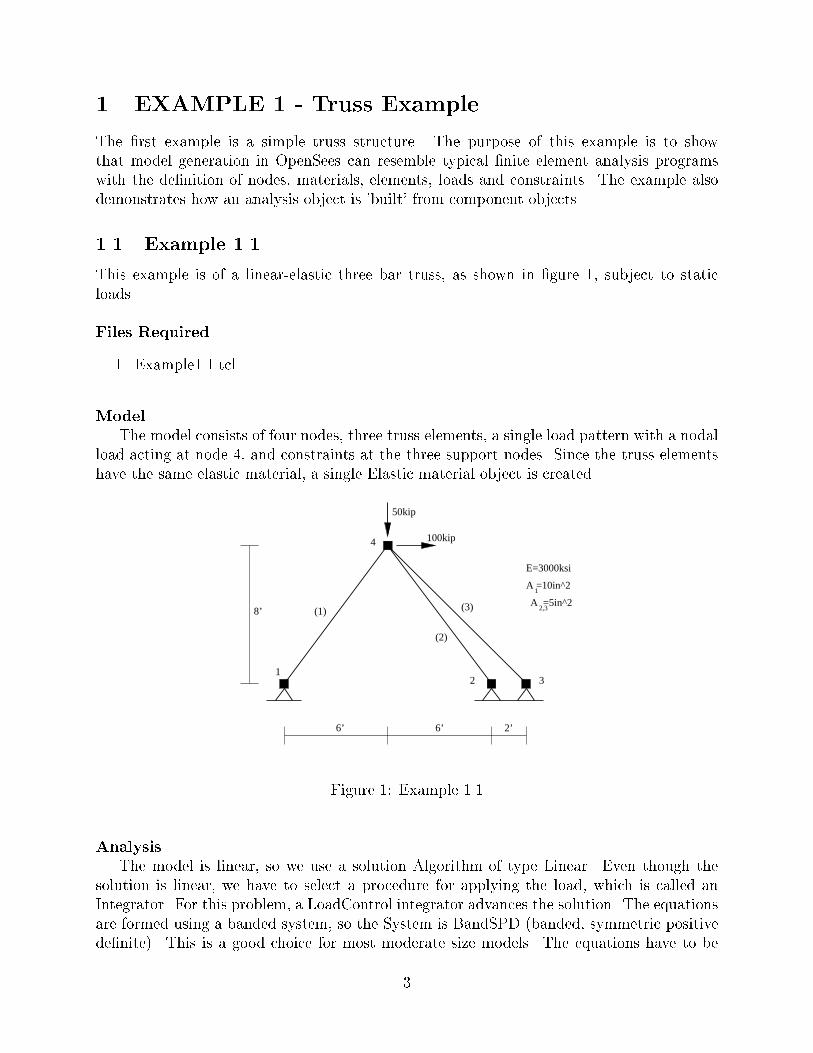
The model consists of two nodes and a ZeroLengthSection element. A depiction of the

element geometry is shown in �gure 2. The drawing on the left of �gure 2 shows an edge

view of the element where the local z-axis, as seen on the right side of the �gure and in

�gure 3, is coming out of the page. Node 1 is completely restrained, while the applied loads

act on node 2. A compressive axial load, P, of 180 kips is applied to the section during the

moment-curvature analysis.

Y

X

��

��

M

P

FixedSteel

Concrete

y

x

Steel

z1 2

y

x

Figure 2: Geometry of zero-length element

7

For the zero length element, a section discretized by concrete and steel is created to

represent the resultant behavior. UniaxialMaterial objects are created to de�ne the �ber

stress-strain relationships: con�ned concrete in the column core, uncon�ned concrete in the

column cover, and reinforcing steel.

The dimensions of the �ber section are shown in �gure 3. The section depth is 24 inches,

the width is 15 inches, and there are 1.5 inches of cover around the entire section. Strong

axis bending is about the section z-axis. In fact, the section z-axis is the strong axis of

bending for all �ber sections in planar problems. The section is separated into con�ned

and uncon�ned concrete regions, for which separate �ber discretizations will be generated.

Reinforcing steel bars will be placed around the boundary of the con�ned and uncon�ned

regions. The �ber discretization for the section is shown in �gure 4.

z

y

depth = 24"

width = 15"

cover = 1.5" cover = 1.5"

cover = 1.5"

Unconfined Region

Confined Region

Figure 3: Dimensions of RC section

��

��

��

��

��

��

��

��

��

��

��

��

��

��

��

��

z

y

(10.5, 6)

(10.5, -6) (-10.5, -6)

(-10.5, 6)

(0, -6)

(0, 6)

Figure 4: Fiber section discretization

8

Analysis

The section analysis is performed by the Tcl procedure MomentCurvature de�ned in the

�le MomentCurvature.tcl. The arguments to the procedure are the tag of the section to be

analyzed, the axial load applied to the section, the maximum curvature, and the number of

displacement increments to reach the maximum curvature.


The output for the moment-curvature analysis will be the section forces and deformations,

stored in the �le section1.out. In addition, an estimate of the section yield curvature is

printed to the screen.

OpenSees Script

In the script below variables, are set and can then be used with the syntax of $variable.

Expressions can be evaluated, although the Tcl syntax at �rst appears cumbersome. An

expression is given by an expr command enclosed in square brackets []'s. Typically, the

result of an expression is then set to another variable. A simple example to add 2.0 to a

parameter is shown below:

set v 3.0

set sum [expr $v + 2.0]

puts $sum; # print the sum

Comments with # can appear on the same line as a command, but then the command

must be terminated with a semi-colon.


# OpenSees Primer

#


# Define model builder

# --------------------


# Define materials for nonlinear columns

# ------------------------------------------

# CONCRETE tag f'c ec0 f'cu ecu

# Core concrete (confined)

uniaxialMaterial Concrete01 1 -6.0 -0.004 -5.0 -0.014

# Cover concrete (unconfined)

uniaxialMaterial Concrete01 2 -5.0 -0.002 0.0 -0.006

# STEEL

# Reinforcing steel

set fy 60.0; # Yield stress

9

set E 30000.0; # Young's modulus

# tag fy E0 b

uniaxialMaterial Steel01 3 $fy $E 0.01

# Define cross-section for nonlinear columns

# ------------------------------------------

# set some parameters

set colWidth 15

set colDepth 24

set cover 1.5

set As 0.60; # area of no. 7 bars

# some variables derived from the parameters

set y1 [expr $colDepth/2.0]

set z1 [expr $colWidth/2.0]

section Fiber 1 {

# Create the concrete core fibers

patch rect 1 10 1 [expr $cover-$y1] [expr $cover-$z1]

[expr $y1-$cover] [expr $z1-$cover]

# Create the concrete cover fibers (top, bottom, left, right)

patch rect 2 10 1 [expr -$y1] [expr $z1-$cover]

$y1 $z1

patch rect 2 10 1 [expr -$y1] [expr -$z1]

$y1 [expr $cover-$z1]

patch rect 2 2 1 [expr -$y1] [expr $cover-$z1]

[expr $cover-$y1] [expr $z1-$cover]

patch rect 2 2 1 [expr $y1-$cover] [expr $cover-$z1]

$y1 [expr $z1-$cover]

# Create the reinforcing fibers (left, middle, right)

layer straight 3 3 $As [expr $y1-$cover] [expr $z1-$cover]

[expr $y1-$cover] [expr $cover-$z1]

layer straight 3 2 $As 0.0 [expr $z1-$cover]

0.0 [expr $cover-$z1]

layer straight 3 3 $As [expr $cover-$y1] [expr $z1-$cover]

[expr $cover-$y1] [expr $cover-$z1]

}

# Estimate yield curvature

# (Assuming no axial load and only top and bottom steel)

set d [expr $colDepth-$cover] ;# d -- from cover to rebar

10

set epsy [expr $fy/$E] ;# steel yield strain

set Ky [expr $epsy/(0.7*$d)]

# Print estimate to standard output

puts "Estimated yield curvature: $Ky"

# Set axial load

set P -180

set mu 15; # Target ductility for analysis

set numIncr 100; # Number of analysis increments

# Call the section analysis procedure

source MomentCurvature.tcl

MomentCurvature 1 $P [expr $Ky*$mu] $numIncr

The Tcl procedure to perform the moment-curvature analysis follows. In this procedure,

the nodes are de�ned to be at the same geometric location and the ZeroLengthSection

element is used. A single load step is performed for the axial load, then the integrator

is changed to DisplacementControl to impose nodal displacements, which map directly to

section deformations. A reference moment of 1.0 is de�ned in a Linear time series. For

this reference moment, the DisplacementControl integrator will determine the load factor

needed to apply the imposed displacement. A node recorder is de�ned to track the moment-

curvature results. The load factor is the moment, and the nodal rotation is in fact the

curvature of the element with zero thickness.

# Arguments

# secTag -- tag identifying section to be analyzed

# axialLoad -- axial load applied to section (negative is compression)

# maxK -- maximum curvature reached during analysis

# numIncr -- number of increments used to reach maxK (default 100)

#

# Sets up a recorder which writes moment-curvature results to file

# section$secTag.out ... the moment is in column 1, and curvature in column 2

proc MomentCurvature {secTag axialLoad maxK {numIncr 100} } {

# Define two nodes at (0,0)

node 1 0.0 0.0

node 2 0.0 0.0

# Fix all degrees of freedom except axial and bending at node 2

fix 1 1 1 1

fix 2 0 1 0

# Define element

# tag ndI ndJ secTag

element zeroLengthSection 1 1 2 $secTag

11

# Create recorder

recorder Node section$secTag.out disp -time -node 2 -dof 3

# Define constant axial load

pattern Plain 1 "Constant" {

load 2 $axialLoad 0.0 0.0

}

# Define analysis parameters

integrator LoadControl 0 1 0 0

system SparseGeneral -piv;

test NormUnbalance 1.0e-9 10

numberer Plain

constraints Plain

algorithm Newton

analysis Static

# Do one analysis for constant axial load

analyze 1

# Define reference moment


load 2 0.0 0.0 1.0

}

# Compute curvature increment

set dK [expr $maxK/$numIncr]

# Use displacement control at node 2 for section analysis

integrator DisplacementControl 2 3 $dK 1 $dK $dK

# Do the section analysis

analyze $numIncr

}

12

Results

Estimated yield curvature: 0.000126984126984

The �le section1.out contains for each committed state a line with the load factor and

the rotation at node 3. This can be used to plot the moment-curvature relationship as shown

in �gure 5.

0 0.2 0.4 0.6 0.8 1 1.2 1.4 1.6 1.8 2

x 10−3

0

500

1000

1500

2000

2500

3000

3500

4000

4500

5000

Curvature (1/in)

Mom

ent (

in*k

ip)

Figure 5: Moment-curvature analysis of column section

13

3 EXAMPLE 3 - Portal Frame Examples

This next set of examples covers the nonlinear analysis of a reinforced concrete frame. The

nonlinear beam column element with a �ber discretization of the cross section is used in

the model. In addition, Tcl language features such as variable and command substitution,

expression evaluation, the if-then-else control structure, and procedures are demonstrated in

several elaborations of the example.

3.1 Example 3.1

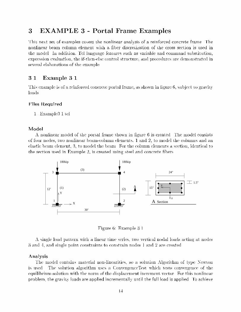
This example is of a reinforced concrete portal frame, as shown in �gure 6, subject to gravity

loads.

Files Required

1. Example3.1.tcl

Model

A nonlinear model of the portal frame shown in �gure 6 is created. The model consists

of four nodes, two nonlinear beam-column elements, 1 and 2, to model the columns and an

elastic beam element, 3, to model the beam. For the column elements a section, identical to

the section used in Example 2, is created using steel and concrete �bers.

1 2

3 4

30’

12’ (1) (2)

(3)

A1.5"

A Section

15"

24"

180kip 180kip

X

Y

y

z


A single load pattern with a linear time series, two vertical nodal loads acting at nodes

3 and 4, and single point constraints to constrain nodes 1 and 2 are created.

Analysis

The model contains material non-linearities, so a solution Algorithm of type Newton

is used. The solution algorithm uses a ConvergenceTest which tests convergence of the

equilibrium solution with the norm of the displacement increment vector. For this nonlinear

problem, the gravity loads are applied incrementally until the full load is applied. To achieve

14

this, a LoadControl integrator which advances the solution with an increment of 0.1 at

each load step is used. The equations are formed using a banded storage scheme, so the

System is BandGeneral. The equations are numbered using an RCM (reverse Cuthill-McKee)

numberer. The constraints are enforced with a Plain constraint handler.


For this problem a Static Analysis object is used. To achieve the full gravity load, 10 load

steps are performed.


At end of analysis, the state at nodes 3 and 4 is output. The state of element 1 is also

output.

OpenSees Script


# OpenSees Primer

#


# ------------------------------


# ------------------------------


model basic -ndm 2 -ndf 3

# Create nodes

# ------------

# Set parameters for overall model geometry

set width 360

set height 144

# Create nodes

# tag X Y

node 1 0.0 0.0

node 2 $width 0.0

node 3 0.0 $height

node 4 $width $height

# Fix supports at base of columns

# tag DX DY RZ

fix 1 1 1 1

fix 2 1 1 1


# ------------------------------------------

15

# CONCRETE tag f'c ec0 f'cu ecu





# STEEL

# Reinforcing steel

set fy 60.0; # Yield stress

set E 30000.0; # Young's modulus

# tag fy E0 b

uniaxialMaterial Steel01 3 $fy $E 0.01


# ------------------------------------------


set colWidth 15

set colDepth 24

set cover 1.5

set As 0.60; # area of no. 7 bars

# some variables derived from the parameters

set y1 [expr $colDepth/2.0]

set z1 [expr $colWidth/2.0]

section Fiber 1 {

# Create the concrete core fibers

patch rect 1 10 1 [expr $cover-$y1] [expr $cover-$z1]

[expr $y1-$cover] [expr $z1-$cover]

# Create the concrete cover fibers (top, bottom, left, right)

patch rect 2 10 1 [expr -$y1] [expr $z1-$cover]

$y1 $z1

patch rect 2 10 1 [expr -$y1] [expr -$z1]

$y1 [expr $cover-$z1]

patch rect 2 2 1 [expr -$y1] [expr $cover-$z1]

[expr $cover-$y1] [expr $z1-$cover]

patch rect 2 2 1 [expr $y1-$cover] [expr $cover-$z1]

$y1 [expr $z1-$cover]

# Create the reinforcing fibers (left, middle, right)

layer straight 3 3 $As [expr $y1-$cover] [expr $z1-$cover]

[expr $y1-$cover] [expr $cover-$z1]

16

layer straight 3 2 $As 0.0 [expr $z1-$cover]

0.0 [expr $cover-$z1]

layer straight 3 3 $As [expr $cover-$y1] [expr $z1-$cover]

[expr $cover-$y1] [expr $cover-$z1]

}

# Define column elements

# ----------------------

# Geometry of column elements

# tag

geomTransf Linear 1

# Number of integration points along length of element

set np 5

# Create the coulumns using Beam-column elements

# tag ndI ndJ nsecs secID transfTag

element nonlinearBeamColumn 1 1 3 $np 1 1

element nonlinearBeamColumn 2 2 4 $np 1 1

# Define beam elment

# -----------------------------

# Geometry of column elements

# tag

geomTransf Linear 2

# Create the beam element

# tag ndI ndJ A E Iz transfTag

element elasticBeamColumn 3 3 4 360 4030 8640 2

# Define gravity loads

# --------------------

# Set some parameter

set P 180; # 10% of axial capacity of columns

# Create a Plain load pattern with a Linear TimeSeries


# Create nodal loads at nodes 3 & 4

# nd FX FY MZ

load 3 0.0 [expr -$P] 0.0

load 4 0.0 [expr -$P] 0.0

}

17

# ------------------------------


# ------------------------------

# ------------------------------


# ------------------------------

# Create the system of equation, a banded general system

system BandGeneral

# Create the constraint handler, the transformation method

constraints Transformation

# Create the DOF numberer, a plain numbering scheme

numberer RCM

# Create the convergence test, the norm of the residual with a tolerance of

# 1e-12 and a max number of iterations of 10

test NormDispIncr 1.0e-12 10 3

# Create the solution algorithm, a Newton-Raphson algorithm

algorithm Newton

# Create the integration scheme, the LoadControl scheme using steps of 0.1


# Create the analysis object

analysis Static

# ------------------------------


# ------------------------------

# ------------------------------


# ------------------------------

# Perform the gravity load analysis, requires 10 steps to reach the load level

analyze 10

# Print out the state of nodes 3 and 4

print node 3 4

18

# Print out the state of element 1

print element 1

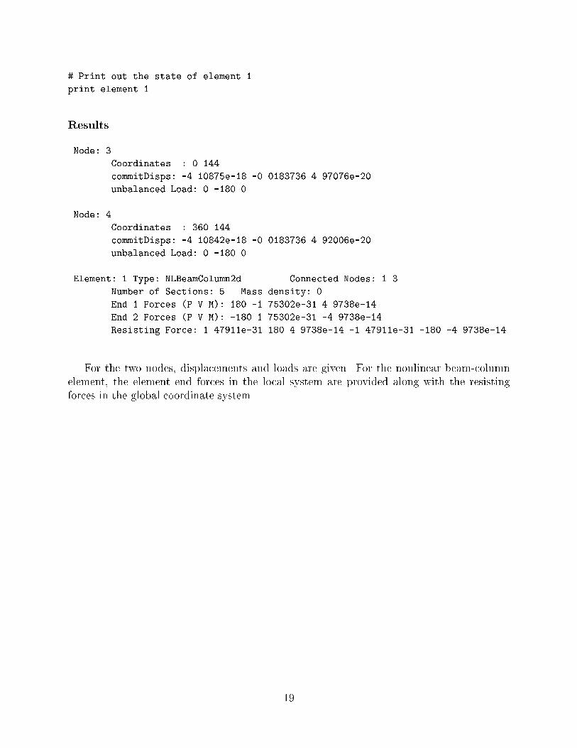
Results

Node: 3

Coordinates : 0 144

commitDisps: -4.10875e-18 -0.0183736 4.97076e-20

unbalanced Load: 0 -180 0

Node: 4

Coordinates : 360 144

commitDisps: -4.10842e-18 -0.0183736 4.92006e-20

unbalanced Load: 0 -180 0

Element: 1 Type: NLBeamColumn2d Connected Nodes: 1 3

Number of Sections: 5 Mass density: 0

End 1 Forces (P V M): 180 -1.75302e-31 4.9738e-14

End 2 Forces (P V M): -180 1.75302e-31 -4.9738e-14

Resisting Force: 1.47911e-31 180 4.9738e-14 -1.47911e-31 -180 -4.9738e-14

For the two nodes, displacements and loads are given. For the nonlinear beam-column

element, the element end forces in the local system are provided along with the resisting

forces in the global coordinate system.

19

3.2 Example 3.2

In this example the nonlinear reinforced concrete portal frame which has undergone the

gravity load analysis of Example 3.1 is now subjected to a pushover analysis.

Files Required

1. Example3.2.tcl

2. Example3.1.tcl

Model

After performing the gravity load analysis on the model, the time in the domain is reset

to 0.0 and the current value of all loads acting are held constant. A new load pattern with a

linear time series and horizontal loads acting at nodes 3 and 4 is then added to the model.

Analysis

The static analysis used to perform the gravity load analysis is modi�ed to take a new

DisplacementControl integrator. At each new step in the analysis the integrator will deter-

mine the load increment necessary to increment the horizontal displacement at node 3 by

0.1 in. 60 analysis steps are performed in this new analysis.


For this analysis the nodal displacements at nodes 3 and 4 will be stored in the �le

nodePushover.out for post-processing. In addition, the end forces in the local coordinate

system for elements 1 and 2 will be stored in the �le elePushover.out. At the end of the

analysis, the state of node 3 is printed to the screen.

OpenSees Script


# OpenSees Primer

#


# ----------------------------------------------------

# Start of Model Generation & Initial Gravity Analysis

# ----------------------------------------------------

# Do operations of Example3.1 by sourcing in the tcl file

source Example3.1.tcl

puts ``Gravity load analysis completed''

# Set the gravity loads to be constant & reset the time in the domain

loadConst -time 0.0

20

# ----------------------------------------------------

# End of Model Generation & Initial Gravity Analysis

# ----------------------------------------------------

# ----------------------------------------------------

# Start of additional modeling for lateral loads

# ----------------------------------------------------

# Define lateral loads

# --------------------

# Set some parameters

set H 10.0; # Reference lateral load

# Set lateral load pattern with a Linear TimeSeries


# Create nodal loads at nodes 3 & 4

# nd FX FY MZ

load 3 $H 0.0 0.0

load 4 $H 0.0 0.0

}

# ----------------------------------------------------

# End of additional modeling for lateral loads

# ----------------------------------------------------

# ----------------------------------------------------

# Start of modifications to analysis for push over

# ----------------------------------------------------


set dU 0.1; # Displacement increment

# Change the integration scheme to be displacement control

# node dof init Jd min max

integrator DisplacementControl 3 1 $dU 1 $dU $dU

# ----------------------------------------------------

# End of modifications to analysis for push over

# ----------------------------------------------------

# ------------------------------

# Start of recorder generation

21

# ------------------------------

# Create a recorder to monitor nodal displacements

recorder Node node32.out disp -time -node 3 4 -dof 1 2 3

# Create a recorder to monitor element forces in columns

recorder Element 1 2 -time -file ele32.out localForce

# --------------------------------

# End of recorder generation

# ---------------------------------

# ------------------------------


# ------------------------------


set maxU 6.0; # Max displacement

set numSteps [expr int($maxU/$dU)]

# Perform the analysis

analyze $numSteps

puts ``Pushover analysis completed''

# Print the state at node 3

print node 3

22

Results

Gravity load analysis completed

Setting time in domain to be : 0.0

Pushover analysis completed

Node: 3

Coordinates : 0 144

commitDisps: 6 0.488625 -0.00851377

unbalanced Load: 71.8819 -180 0

In addition to what is displayed on the screen, the �le node32.out and ele32.out have

been created by the script. Each line of node32.out contains the time, DX, DY and RZ for

node 3 and DX, DY and RZ for node 4 at the end of an iteration. Each line of eleForce.out

contains the time, and the element end forces in the local coordinate system. A plot of the

load-displacement relationship at node 3 is shown in �gure 7.

0 1 2 3 4 5 620

40

60

80

100

120

140

160

Lateral Displacement (in)

Tot

al L

ater

al L

oad

(kip

)

Figure 7: Load displacement curve for node 3

23

3.3 Example 3.3

In this example the reinforced concrete portal frame which has undergone the gravity load

analysis of Example 3.1 is now subjected to a uniform earthquake excitation.

Files Required

1. Example3.3.tcl

2. Example3.1.tcl

3. ReadSMDFile.tcl

Model

After performing the gravity load analysis, the time in the domain is reset to 0.0 and the

current value of all active loads is set to constant. Mass terms are added to nodes 3 and 4.

A new uniform excitation load pattern is created. The excitation acts in the horizontal di-

rection and reads the acceleration record and time interval from the �le ARL360.g3. The �le

ARL360.g3 is created from the PEER Strong Motion Database (http://peer.berkeley.edu/smcat/)

record ARL360.at2 using the Tcl procedure ReadSMDFile contained in the �le ReadSMD-

File.tcl.

Analysis

The static analysis object and its components are �rst deleted so that a new transient

analysis object can be created.

A new solution Algorithm of type Newton is then created. The solution algorithm uses a

ConvergenceTest which tests convergence on the norm of the displacement increment vector.

The integrator for this analysis will be of type Newmark with a of 0.25 and a � of 0.5.

The integrator will add some sti�ness proportional damping to the system, the damping

term will be based on the last committed stifness of the elements, i.e. C = acKcommit

with ac = 0:000625. The equations are formed using a banded storage scheme, so the

System is BandGeneral. The equations are numbered using an RCM (reverse Cuthill-McKee)

numberer. The constraints are enforced with a Plain constraint handler.


For this problem a Transient Analysis object is used. 2000 time steps are performed with a

time step of 0.01.

In addition to the transient analysis, two eigenvalue analysis are performed on the model.

The �rst is performed after the gravity analysis and the second after the transient analysis.


For this analysis the nodal displacenments at Nodes 3 and 4 will be stored in the �le

nodeTransient.out for post-processing. In addition the section forces and deformations for

the section at the base of column 1 will also be stored in two seperate �les. The results of

the eigenvalue analysis will be displayed on the screen.

OpenSees Script

24


# OpenSees Primer

#


# ----------------------------------------------------

# Start of Model Generation & Initial Gravity Analysis

# ----------------------------------------------------

# Do operations of Example3.1 by sourcing in the tcl file

source Example3.1.tcl

puts ``Gravity load analysis completed''

# Set the gravity loads to be constant & reset the time in the domain

loadConst -time 0.0

# ----------------------------------------------------

# End of Model Generation & Initial Gravity Analysis

# ----------------------------------------------------

# ----------------------------------------------------

# Start of additional modeling for dynamic loads

# ----------------------------------------------------

# Define nodal mass in terms of axial load on columns

set g 386.4

set m [expr $P/$g]; # expr command to evaluate an expression

# tag MX MY RZ

mass 3 $m $m 0

mass 4 $m $m 0

# Define dynamic loads

# --------------------


set outFile ARL360.g3

set accelSeries "Path -filePath $outFile -dt $dt -factor $g"

# Source in TCL proc to read a PEER Strong Motion Database record

source ReadSMDFile.tcl

# Perform the conversion from SMD record to OpenSees record and obtain dt

# inFile outFile dt

ReadSMDFile ARL360.at2 $outFile dt

# Create UniformExcitation load pattern

25

# tag dir

pattern UniformExcitation 2 1 -accel $accelSeries

# ----------------------------------------------------

# End of additional modeling for dynamic loads

# ----------------------------------------------------

# ---------------------------------------------------------

# Start of modifications to analysis for transient analysis

# ---------------------------------------------------------

# Delete the old analysis and all its component objects

wipeAnalysis



test NormDispIncr 1.0e-12 10


algorithm Newton

# Create the integration scheme, Newmark with gamma = 0.5 and beta = 0.25

integrator Newmark 0.5 0.25 0.0 0.0 0.0 0.000625

# Create the system of equation, a banded general storage scheme

system BandGeneral

# Create the constraint handler, a plain handler as homogeneous boundary conditions

constraints Plain


numberer RCM


analysis Transient

# ---------------------------------------------------------

# End of modifications to analysis for transient analysis

# ---------------------------------------------------------

# ------------------------------


# ------------------------------

# Create a recorder to monitor nodal displacements

recorder Node nodeTransient.out disp -time -node 3 -dof 1 2 3

26

# Create recorders to monitor section forces and deformations

# at the base of the left column

recorder Element 1 -time -file ele1secForce.out section 1 force

recorder Element 1 -time -file ele1secDef.out section 1 deformation

# --------------------------------


# ---------------------------------

# ------------------------------


# ------------------------------

# Perform an eigenvalue analysis

eigen 2

# Perform the transient analysis

# N dt

analyze 2000 0.01

# Perform an eigenvalue analysis

eigen 2

# Print state of node 3

print node 3

27

Results

Gravity load analysis completed

Setting time in domain to be : 0.0

Eigenvalues: 269.542 17507.1

Transient analysis completed

Eigenvalues: 165.873 17326.1

Node: 3

Coordinates : 0 144

commitDisps: -0.105551 -0.0217913 0.000601786

Velocities : -1.54243 0.0252537 0.00986257

commitAccels: 5.0767 0.249952 1.47823

unbalanced Load: -3.9475 -180 0

Mass :

0.465839 0 0

0 0.465839 0

0 0 0

Eigenvectors:

-1.03574 -0.954357

0.0131099 0.283352

0.00666553 0.00463143

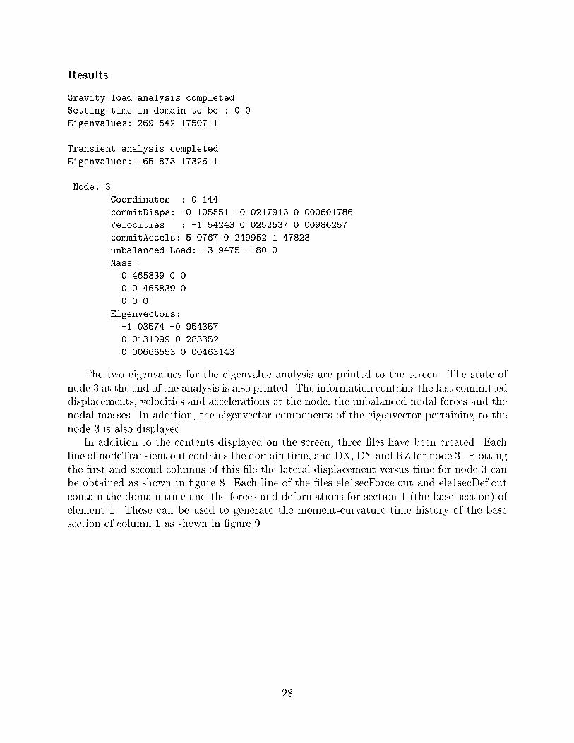
The two eigenvalues for the eigenvalue analysis are printed to the screen. The state of

node 3 at the end of the analysis is also printed. The information contains the last committed

displacements, velocities and accelerations at the node, the unbalanced nodal forces and the

nodal masses. In addition, the eigenvector components of the eigenvector pertaining to the

node 3 is also displayed.

In addition to the contents displayed on the screen, three �les have been created. Each

line of nodeTransient.out contains the domain time, and DX, DY and RZ for node 3. Plotting

the �rst and second columns of this �le the lateral displacement versus time for node 3 can

be obtained as shown in �gure 8. Each line of the �les ele1secForce.out and ele1secDef.out

contain the domain time and the forces and deformations for section 1 (the base section) of

element 1. These can be used to generate the moment-curvature time history of the base

section of column 1 as shown in �gure 9.

28

0 2 4 6 8 10 12 14 16 18 20−2

−1.5

−1

−0.5

0

0.5

1

1.5

2

Time (sec)

Late

rial D

ispl

acem

ent (

in)

Figure 8: Lateral displacement at node 3

−1.5 −1 −0.5 0 0.5 1 1.5 2

x 10−3

−6000

−4000

−2000

0

2000

4000

6000

Curvature (1/in)

Mom

ent (

in*k

ip)

Element 1 Base Section

Figure 9: Column section moment-curvature results

29

4 EXAMPLE 4 - Multibay Two Story Frame Example

In this next example the use of variable substitution and the Tcl loop control structure for

building models is demonstrated.

4.1 Example 4.1

This example is of a reinforced concrete multibay two story frame, as shown in �gure 10,

subject to gravity loads.

Files Required

1. Example4.1.tcl

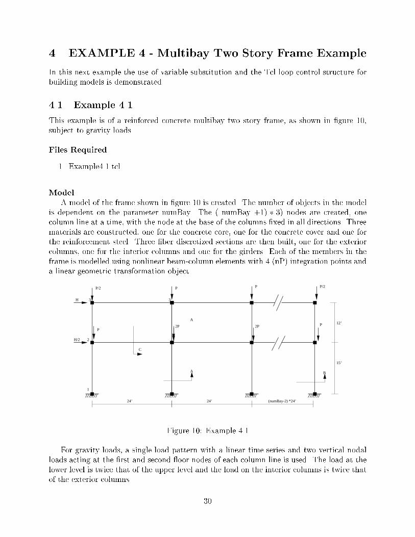
Model

A model of the frame shown in �gure 10 is created. The number of objects in the model

is dependent on the parameter numBay. The ( numBay +1) � 3) nodes are created, one

column line at a time, with the node at the base of the columns �xed in all directions. Three

materials are constructed, one for the concrete core, one for the concrete cover and one for

the reinforcement steel. Three �ber discretized sections are then built, one for the exterior

columns, one for the interior columns and one for the girders. Each of the members in the

frame is modelled using nonlinear beam-column elements with 4 (nP) integration points and

a linear geometric transformation object.

A

A

P/2 P

2P

H

H/2

24’

3

1

24’

P

3

2

2P

P/2

P

P

(numBay-2) *24’

B

C

12’

15’


For gravity loads, a single load pattern with a linear time series and two vertical nodal

loads acting at the �rst and second oor nodes of each column line is used. The load at the

lower level is twice that of the upper level and the load on the interior columns is twice that

of the exterior columns.

30

For the lateral load analysis, a second load pattern with a linear time series is introduced

after the gravity load analysis. Associated with this load pattern are two nodal loads acting

on nodes 2 and 3, with the load level at node 3 twice that acting at node 2.

Analysis

A solution Algorithm of type Newton is created. The solution algorithm uses a Conver-

genceTest based on the norm of the displacement increment vector. The integrator for the

analysis will be LoadControl with a load step increment of 0.1. The storage for the system

of equations is BandGeneral. The equations are numbered using an RCM (reverse Cuthill-

McKee) numberer. The constraints are enforced with a Plain constraint handler. Once the

components of the analysis have been de�ned, the analysis object is then created. For this

problem a Static analysis object is used and 10 steps are performed to load the model with

the desired gravity load.

After the gravity load analysis has been performed, the gravity loads are set to constant

and the time in the domain is reset to 0.0. A new LoadControl integrator is now added. The

new LoadControl integrator has an initial load step of 1.0, but this can vary between 0.02

and 2.0 depending on the number of iterations required to achieve convergence at each load

step. 100 steps are then performed.


For the pushover analysis the lateral displacements at nodes 2 and 3 will be stored in

the �le Node41.out for post-processing. In addition, if the variable displayMode is set to

\displayON" the load-displacement curve for horizontal displacements at node 3 will be

displayed in a window on the user's terminal.

OpenSees Script


# OpenSees Primer

#


# Parameter identifying the number of bays

set numBay 3

# ------------------------------


# ------------------------------



# Create nodes

# ------------

# Set parameters for overall model geometry

31

set bayWidth 288

set nodeID 1

# Define nodes

for {set i 0} {$i <= $numBay} {incr i 1} {

set xDim [expr $i * $bayWidth]

# tag X Y

node $nodeID $xDim 0

node [expr $nodeID+1] $xDim 180

node [expr $nodeID+2] $xDim 324

incr nodeID 3

}

# Fix supports at base of columns


# node DX DY RZ

fix [expr $i*3+1] 1 1 1

}


# ------------------------------------------

# CONCRETE

# Cover concrete

# tag -f'c -epsco -f'cu -epscu


# Core concrete


# STEEL

# Reinforcing steel

# tag fy E0 b

uniaxialMaterial Steel01 3 60 30000 0.02


# ------------------------------------------

# Interior column section - Section A

section Fiber 1 {

# mat nfIJ nfJK yI zI yJ zJ yK zK yL zL

patch quadr 2 1 12 -11.5 10 -11.5 -10 11.5 -10 11.5 10

patch quadr 1 1 14 -13.5 -10 -13.5 -12 13.5 -12 13.5 -10

patch quadr 1 1 14 -13.5 12 -13.5 10 13.5 10 13.5 12

32

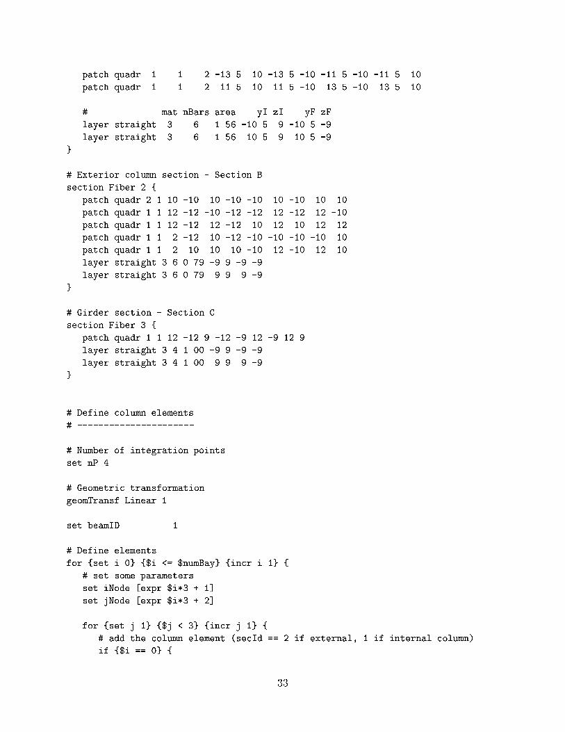
patch quadr 1 1 2 -13.5 10 -13.5 -10 -11.5 -10 -11.5 10

patch quadr 1 1 2 11.5 10 11.5 -10 13.5 -10 13.5 10

# mat nBars area yI zI yF zF

layer straight 3 6 1.56 -10.5 9 -10.5 -9

layer straight 3 6 1.56 10.5 9 10.5 -9

}

# Exterior column section - Section B

section Fiber 2 {

patch quadr 2 1 10 -10 10 -10 -10 10 -10 10 10

patch quadr 1 1 12 -12 -10 -12 -12 12 -12 12 -10

patch quadr 1 1 12 -12 12 -12 10 12 10 12 12

patch quadr 1 1 2 -12 10 -12 -10 -10 -10 -10 10

patch quadr 1 1 2 10 10 10 -10 12 -10 12 10

layer straight 3 6 0.79 -9 9 -9 -9

layer straight 3 6 0.79 9 9 9 -9

}

# Girder section - Section C

section Fiber 3 {

patch quadr 1 1 12 -12 9 -12 -9 12 -9 12 9

layer straight 3 4 1.00 -9 9 -9 -9

layer straight 3 4 1.00 9 9 9 -9

}


# ----------------------

# Number of integration points

set nP 4

# Geometric transformation

geomTransf Linear 1

set beamID 1

# Define elements



set iNode [expr $i*3 + 1]

set jNode [expr $i*3 + 2]

for {set j 1} {$j < 3} {incr j 1} {

# add the column element (secId == 2 if external, 1 if internal column)

if {$i == 0} {

33

element nonlinearBeamColumn $beamID $iNode $jNode $nP 2 1

} elseif {$i == $numBay} {


} else {


}

# increment the parameters

incr iNode 1

incr jNode 1

incr beamID 1

}

}

# Define beam elements

# ----------------------

# Number of integration points

set nP 4

# Geometric transformation

geomTransf Linear 2

# Define elements

for {set j 1} {$j < 3} {incr j 1} {


set iNode [expr $j + 1]

set jNode [expr $iNode + 3]



# increment the parameters

incr iNode 3

incr jNode 3

incr beamID 1

}

}


# --------------------

# Constant gravity load

set P -192


34

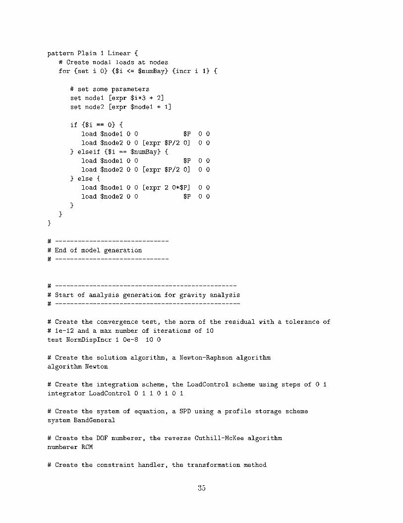
pattern Plain 1 Linear {

# Create nodal loads at nodes



set node1 [expr $i*3 + 2]

set node2 [expr $node1 + 1]

if {$i == 0} {

load $node1 0.0 $P 0.0

load $node2 0.0 [expr $P/2.0] 0.0

} elseif {$i == $numBay} {


load $node2 0.0 [expr $P/2.0] 0.0

} else {

load $node1 0.0 [expr 2.0*$P] 0.0


}

}

}

# ------------------------------


# ------------------------------

# ------------------------------------------------

# Start of analysis generation for gravity analysis

# -------------------------------------------------



test NormDispIncr 1.0e-8 10 0


algorithm Newton

# Create the integration scheme, the LoadControl scheme using steps of 0.1


# Create the system of equation, a SPD using a profile storage scheme

system BandGeneral


numberer RCM

# Create the constraint handler, the transformation method

35

constraints Plain


analysis Static

# ------------------------------------------------

# End of analysis generation for gravity analysis

# -------------------------------------------------

# ------------------------------

# Perform gravity load analysis

# ------------------------------

# perform the gravity load analysis, requires 10 steps to reach the load level

analyze 10

# set gravity loads to be const and set pseudo time to be 0.0

# for start of lateral load analysis

loadConst -time 0.0

# ------------------------------

# Add lateral loads

# ------------------------------

# Reference lateral load for pushover analysis

set H 10

# Reference lateral loads


pattern Plain 2 Linear {

load 2 [expr $H/2.0] 0.0 0.0

load 3 $H 0.0 0.0

}

# ------------------------------


# ------------------------------

# Create a recorder which writes to Node.out and prints

# the current load factor (pseudo-time) and dof 1 displacements at node 2 & 3

recorder Node Node41.out disp -time -node 2 3 -dof 1

# Source in some commands to display the model

36

# comment out one of lines

set displayMode "displayON"

#set displayMode "displayOFF"

if {$displayMode == "displayON"} {

# a window to plot the nodal displacements versus load for node 3

recorder plot Node41.out Node3Xdisp 10 340 300 300 -columns 3 1

}

# ------------------------------


# ------------------------------

# ------------------------------

# Start of lateral load analysis

# ------------------------------

# Change the integrator to take a min and max load increment



analyze 100

Results

The output consists of the �le Node41.out containing a line for each step of the lateral

load analysis. Each line contains the load factor, the lateral displacements at nodes 2 and

3. A plot of the load-displacement curve for the frame is given in �gure 11.

37

0 0.5 1 1.5 2 2.5 3 3.5 40

50

100

150

200

250

300

350

400

450

500

Displacement (in)

Tot

al L

ater

al L

oad

(kip

)

Load−Displacement of Two Story Frame

Figure 11: Pushover curve for two-story three-bay frame

38

5 EXAMPLE 5 - Three-Dimensional Rigid Frame

5.1 Example 5.1

This example is of a three-dimensional reinforced concrete rigid frame, as shown in �gure 12,

subjected to bi-directional earthquake ground motion.

Files Required

1. Example5.1.tcl

2. RCsection.tcl

3. tabasFN.txt

4. tabasFP.txt

Model

A model of the rigid frame shown in �gure 12 is created. The model consists of three

stories and one bay in each direction. Rigid diaphragm multi-point constraints are used to

enforce the rigid in-plane sti�ness assumption for the oors. Gravity loads are applied to the

structure and the 1978 Tabas acceleration records are the uniform earthquake excitations.

Nonlinear beam column elements are used for all members in the structure. The beam

sections are elastic while the column sections are discretized by �bers of concrete and steel.

Elastic beam column elements may have been used for the beam members; but, it is useful to

see that section models other than �ber sections may be used in the nonlinear beam column

element.

Analysis

A solution Algorithm of type Newton is used for the nonlinear problem. The solution

algorithm uses a ConvergenceTest which tests convergence on the norm of the energy incre-

ment vector. The integrator for this analysis will be of type Newmark with a of 0.25 and

a � of 0.5. Due to the presence of the multi-point constraints, a Transformation constraint

handler is used. The equations are formed using a sparse storage scheme which will perform

pivoting during the equation solving, so the System is SparseGeneral. As SparseGeneral will

perform it's own internal numbering of the equations, a Plain numberer is used which simply

assigns equation numbers to the degrees-of-freedom.


For this problem a Transient Analysis object is used. 2000 steps are performed with a time

step of 0.01.


The nodal displacements at nodes 9, 14, and 19 (the master nodes for the rigid di-

aphragms) will be stored in the �le node51.out for post-processing.

OpenSees Script

39

(1) (2)

(3)

(4)

12’

12’

12’

20’

20’

Z

X

Y

(5)

(10)

(15)

(6)

(8)

(11)

(13)

(16)

(18) (19)

(14)

(9)

(7)

(12)

(17)



# OpenSees Primer

#


# ----------------------------


# ----------------------------

# Create ModelBuilder with 3 dimensions and 6 DOF/node


# Define geometry

# ---------------

# Set parameters for model geometry

set h 144.0; # Story height

set by 240.0; # Bay width in Y-direction

set bx 240.0; # Bay width in X-direction

# Create nodes

# tag X Y Z

node 1 [expr -$bx/2] [expr $by/2] 0

40

node 2 [expr $bx/2] [expr $by/2] 0

node 3 [expr $bx/2] [expr -$by/2] 0

node 4 [expr -$bx/2] [expr -$by/2] 0

node 5 [expr -$bx/2] [expr $by/2] $h

node 6 [expr $bx/2] [expr $by/2] $h

node 7 [expr $bx/2] [expr -$by/2] $h

node 8 [expr -$bx/2] [expr -$by/2] $h

node 10 [expr -$bx/2] [expr $by/2] [expr 2*$h]

node 11 [expr $bx/2] [expr $by/2] [expr 2*$h]

node 12 [expr $bx/2] [expr -$by/2] [expr 2*$h]

node 13 [expr -$bx/2] [expr -$by/2] [expr 2*$h]

node 15 [expr -$bx/2] [expr $by/2] [expr 3*$h]

node 16 [expr $bx/2] [expr $by/2] [expr 3*$h]

node 17 [expr $bx/2] [expr -$by/2] [expr 3*$h]

node 18 [expr -$bx/2] [expr -$by/2] [expr 3*$h]

# Master nodes for rigid diaphragm

# tag X Y Z

node 9 0 0 $h

node 14 0 0 [expr 2*$h]

node 19 0 0 [expr 3*$h]

# Set base constraints

# tag DX DY DZ RX RY RZ

fix 1 1 1 1 1 1 1

fix 2 1 1 1 1 1 1

fix 3 1 1 1 1 1 1

fix 4 1 1 1 1 1 1

# Define rigid diaphragm multi-point constraints

# normalDir master slaves

rigidDiaphragm 3 9 5 6 7 8



# Constraints for rigid diaphragm master nodes

# tag DX DY DZ RX RY RZ

fix 9 0 0 1 1 1 0

fix 14 0 0 1 1 1 0

fix 19 0 0 1 1 1 0


# --------------------------------------

# CONCRETE

41


# tag f'c epsc0 f'cu epscu



set fc 4.0

uniaxialMaterial Concrete01 2 -$fc -0.002 0.0 -0.006

# STEEL

# Reinforcing steel

# tag fy E b

uniaxialMaterial Steel01 3 60 30000 0.02

# Column width

set d 18.0

# Source in a procedure for generating an RC fiber section

source RCsection.tcl

# Call the procedure to generate the column section

# id h b cover core cover steel nBars area nfCoreY nfCoreZ nfCoverY nfCoverZ

RCsection 1 $d $d 2.5 1 2 3 3 0.79 8 8 10 10

# Concrete elastic stiffness

set E [expr 57000.0*sqrt($fc*1000)/1000];

# Column torsional stiffness

set GJ 1.0e10;

# Linear elastic torsion for the column

uniaxialMaterial Elastic 10 $GJ

# Attach torsion to the RC column section

# tag uniTag uniCode secTag

section Aggregator 2 10 T -section 1

set colSec 2


# ----------------------

#set PDelta "ON"

set PDelta "OFF"

# Geometric transformation for columns

if {$PDelta == "ON"} {

# tag vecxz

geomTransf LinearWithPDelta 1 1 0 0

} else {

42

geomTransf Linear 1 1 0 0

}

# Number of column integration points (sections)

set np 4

# Create the nonlinear column elements

# tag ndI ndJ nPts secID transf

element nonlinearBeamColumn 1 1 5 $np $colSec 1












# Define beam elements

# --------------------

# Define material properties for elastic beams

# Using beam depth of 24 and width of 18

# --------------------------------------------

set Abeam [expr 18*24];

# "Cracked" second moments of area

set Ibeamzz [expr 0.5*1.0/12*18*pow(24,3)];

set Ibeamyy [expr 0.5*1.0/12*24*pow(18,3)];

# Define elastic section for beams

# tag E A Iz Iy G J

section Elastic 3 $E $Abeam $Ibeamzz $Ibeamyy $GJ 1.0

set beamSec 3

# Geometric transformation for beams

# tag vecxz

geomTransf Linear 2 1 1 0

# Number of beam integration points (sections)

set np 3

# Create the beam elements

43

# tag ndI ndJ nPts secID transf

element nonlinearBeamColumn 13 5 6 $np $beamSec 2













# --------------------

# Gravity load applied at each corner node

# 10% of column capacity

set p [expr 0.1*$fc*$h*$h]

# Mass lumped at master nodes

set g 386.4; # Gravitational constant

set m [expr (4*$p)/$g]

# Rotary inertia of floor about master node

set i [expr $m*($bx*$bx+$by*$by)/12.0]

# Set mass at the master nodes

# tag MX MY MZ RX RY RZ

mass 9 $m $m 0 0 0 $i

mass 14 $m $m 0 0 0 $i

mass 19 $m $m 0 0 0 $i


pattern Plain 1 Constant {

foreach node {5 6 7 8 10 11 12 13 15 16 17 18} {

load $node 0.0 0.0 -$p 0.0 0.0 0.0

}

}

# Define earthquake excitation

# ----------------------------

# Set up the acceleration records for Tabas fault normal and fault parallel

set tabasFN "Path -filePath tabasFN.txt -dt 0.02 -factor $g"

set tabasFP "Path -filePath tabasFP.txt -dt 0.02 -factor $g"

44

# Define the excitation using the Tabas ground motion records

# tag dir accel series args

pattern UniformExcitation 2 1 -accel $tabasFN

pattern UniformExcitation 3 2 -accel $tabasFP

# -----------------------


# -----------------------

# ----------------------------


# ----------------------------

# Create the convergence test

# tol maxIter printFlag

test EnergyIncr 1.0e-8 20 3

# Create the solution algorithm

algorithm Newton

# Create the system of equation storage and solver

system SparseGeneral -piv

# Create the constraint handler

constraints Transformation

# Create the time integration scheme

# gamma beta

integrator Newmark 0.5 0.25

# Create the DOF numberer

numberer RCM

# Create the transient analysis

analysis Transient

# --------------------------


# --------------------------

# ----------------------------


# ----------------------------

45

# Record DOF 1 and 2 displacements at nodes 9, 14, and 19

recorder Node node51.out disp -time -node 9 14 19 -dof 1 2

# --------------------------


# --------------------------

# --------------------


# --------------------

# Analysis duration of 20 seconds

# numSteps dt

analyze 2000 0.01

Results

The results consist of the �le node51.out, which contains a line for every time step. Each

line contains the time and the horizontal and vertical displacements at the diaphragm master

nodes (9, 14 and 19) i.e. time Dx9 Dy9 Dx14 Dy14 Dx19 Dy19. The horizontal displacement

time history of the �rst oor diaphragm node 9 is shown in �gure 13. Notice the increase in

period after about 10 seconds of earthquake excitation, when the large pulse in the ground

motion propogates through the structure. The displacement pro�le over the three stories

shows a soft-story mechanism has formed in the �rst oor columns. The numerical solution

converges even though the drift is � 20%. The inclusion of P-Delta e�ects shows structural

collapse under such large drifts.

0 2 4 6 8 10 12 14 16 18 20−70

−60

−50

−40

−30

−20

−10

0

10

20

30

Time (sec)

Dis

plac

emen

t (in

)

Linear P−∆

Figure 13: Node 9 displacement time history

46

Open Sees Examples 2001

Documents

analysis procedure

analysis object foranalyzing

features of opensees

transient nonlinear

typical examples

onhow opensees

simple static linear

modelbuilder object