1 SC/63/IA9 Open sea area in the south of the ice edge in IDCR/SOWER CPII and CPIII HIROTO MURASE 1 , KOJI MATSUOKA 1 , TAKASHI HAKAMADA 1 , SHIGETOSHI NISHIWAKI 1 , ATSUSHI WADA 1 AND TOSHIHIDE KITAKADO 2 1 The Institute of Cetacean Research, 4-5 Toyomi-cho, Chuo-ku, Tokyo, 104-0055, Japan 2 Tokyo University of Marine Science and Technology, 4-5-7 Konan, Minato-ku, Tokyo, 108-8477, Japan ABSTRACT Open sea area in the south of the ice edge in IDCR/SOWER CPII and CPIII was calculated by using sighting effort data and sea ice data derived by satellite. First, start and end dates in each 5º longitudinal sector were identified using sighting effort data. Then, mean sea ice concentrations in the south of the ice edge in each 5º longitudinal sector were calculated based on the dates. Finally, Open sea area in the south of the ice edge in each 5º longitudinal sector was calculated. The data prepared by this exercise will be used as a basis for estimation of number of Antarctic minke whales in the south of ice edge. As previously reported, sea ice conditions in the south of the ice edge were varied in both regions and years. In addition, other environmental conditions and number of other baleen whales were different between CPII and CPIII in some regions. Region-specific integrated approach should be taken to estimate number of animals in the south of the ice edge because factors affecting abundance estimate are different from region to region. Development of appropriate model to estimate number of animals in the south of the ice edge is critically important. INTRODUCTION The International Whaling Commission (IWC) conducted sighting surveys for assessing the abundance of the Antarctic minke whale (Balaenoptera bonaerensis) from 1978/79 to 2009/10 in the Antarctic in austral summer (Matsuoka et al., 2003 for review). The names of the cruises were firstly the International Decade of Cetacean Research programme (IDCR, from 1978/79 to 1995/96) and then the Southern Ocean Whale and Ecosystem Research programme (SOWER, from 1996/97 to 2009/10). These cruises covered three circumpolar surveys for the purpose of comprehensive assessments: 1978/79-1983/84 (first circumpolar, CPI), 1984/85-1990/91 (second circumpolar, CPII) and 1991/92-2003/2004 (third circumpolar, CPIII). Abundance estimates based on the IWC standard method revealed that an appreciable difference between CPII and CPIII (Branch and Butterworth, 2001; Branch, 2006). The reasons of the difference have been investigated by the Scientific Committee of the IWC (IWC/SC) since 2001 (IWC, 2002a) but conclusion has not been reached. Number of animals in the south of the ice edge where IDCR/SOWER research vessels could not conduct surveys has been identified as one of the reasons of the difference (IWC, 2002b; IWC, 2003b). Several studies were attempted to estimate number of animals in the south of the ice edge by using IDCR/SOWER data and sea ice data derived from satellite (e.g. Shimada et al., 2001). However, they used not open sea ice area in the south of the ice edge but sea ice extent. Because Antarctic minke whales are distributed in the open sea area in the south of ice edge, use of open sea area in the south of ice edge rather than sea ice extent is appropriate to estimate number of animals. In this paper, open sea ice area in the south of ice edge in each IWC management area by 5º longitudinal sector in CPII and CPIII are presented. This exercise was conducted based on the recommendation of the 62nd IWC/SC (IWC, 2011). MATERIALS AND METHODS Sighting effort and stratum boundary data prepared as a standard data (Burt, 2004) were used in this analysis. Sighting effort data were separated in 1 km segments and aggregated in 5º longitudinal sectors to identified start and end dates of the survey in the sectors. More than one survey was conducted in same longitudinal sector in CPIII. Survey-once option described in Branch (2005) was used to determine 5º longitudinal sectors in this paper. Ice edges in this paper were the southern boundaries of the IDCR/SOWER survey areas determined by the cruise leaders and defined by a level of ice cover that prevented the survey from being conducted at nominal survey speed of 11.5 knots (IWC, 2003a). Areas between the ice edges and the coast line of Antarctica were identified as sea ice area. The coast line in Antarctic Digital Database version 3 provided by the Scientific Committee on Antarctic Research (SCAR) was used. Polygons of the sea ice areas were prepared using a geographic information system (GIS) software, ArcGIS (Version 9.3.1). Satellite derived daily sea ice data, Bootstrap Sea Ice Concentrations from Nimbus-7 SMMR and DMSP SSM/I (Comiso, 1999) from 1978 to 2004 was used in the analysis. The data was provided by the National Snow and Ice Data Center (NSIDC, US). Sea ice observation using the satellite passive microwave sensors was started

Welcome message from author
This document is posted to help you gain knowledge. Please leave a comment to let me know what you think about it! Share it to your friends and learn new things together.
Transcript
1
SC/63/IA9
Open sea area in the south of the ice edge in
IDCR/SOWER CPII and CPIII
HIROTO MURASE1, KOJI MATSUOKA
1, TAKASHI HAKAMADA
1, SHIGETOSHI NISHIWAKI
1, ATSUSHI WADA
1 AND
TOSHIHIDE KITAKADO2
1 The Institute of Cetacean Research, 4-5 Toyomi-cho, Chuo-ku, Tokyo, 104-0055, Japan
2 Tokyo University of Marine Science and Technology, 4-5-7 Konan, Minato-ku, Tokyo, 108-8477, Japan
ABSTRACT
Open sea area in the south of the ice edge in IDCR/SOWER CPII and CPIII was calculated by using sighting effort data and sea
ice data derived by satellite. First, start and end dates in each 5º longitudinal sector were identified using sighting effort data. Then, mean sea ice concentrations in the south of the ice edge in each 5º longitudinal sector were calculated based on the dates. Finally,
Open sea area in the south of the ice edge in each 5º longitudinal sector was calculated. The data prepared by this exercise will be
used as a basis for estimation of number of Antarctic minke whales in the south of ice edge. As previously reported, sea ice conditions in the south of the ice edge were varied in both regions and years. In addition, other environmental conditions and
number of other baleen whales were different between CPII and CPIII in some regions. Region-specific integrated approach should be taken to estimate number of animals in the south of the ice edge because factors affecting abundance estimate are
different from region to region. Development of appropriate model to estimate number of animals in the south of the ice edge is
critically important.
INTRODUCTION
The International Whaling Commission (IWC) conducted sighting surveys for assessing the abundance of the
Antarctic minke whale (Balaenoptera bonaerensis) from 1978/79 to 2009/10 in the Antarctic in austral summer
(Matsuoka et al., 2003 for review). The names of the cruises were firstly the International Decade of Cetacean
Research programme (IDCR, from 1978/79 to 1995/96) and then the Southern Ocean Whale and Ecosystem
Research programme (SOWER, from 1996/97 to 2009/10). These cruises covered three circumpolar surveys for
the purpose of comprehensive assessments: 1978/79-1983/84 (first circumpolar, CPI), 1984/85-1990/91 (second
circumpolar, CPII) and 1991/92-2003/2004 (third circumpolar, CPIII). Abundance estimates based on the IWC
standard method revealed that an appreciable difference between CPII and CPIII (Branch and Butterworth, 2001;
Branch, 2006). The reasons of the difference have been investigated by the Scientific Committee of the IWC
(IWC/SC) since 2001 (IWC, 2002a) but conclusion has not been reached. Number of animals in the south of the
ice edge where IDCR/SOWER research vessels could not conduct surveys has been identified as one of the
reasons of the difference (IWC, 2002b; IWC, 2003b). Several studies were attempted to estimate number of
animals in the south of the ice edge by using IDCR/SOWER data and sea ice data derived from satellite (e.g.
Shimada et al., 2001). However, they used not open sea ice area in the south of the ice edge but sea ice extent.
Because Antarctic minke whales are distributed in the open sea area in the south of ice edge, use of open sea area
in the south of ice edge rather than sea ice extent is appropriate to estimate number of animals. In this paper,
open sea ice area in the south of ice edge in each IWC management area by 5º longitudinal sector in CPII and
CPIII are presented. This exercise was conducted based on the recommendation of the 62nd IWC/SC (IWC,
2011).
MATERIALS AND METHODS
Sighting effort and stratum boundary data prepared as a standard data (Burt, 2004) were used in this analysis.
Sighting effort data were separated in 1 km segments and aggregated in 5º longitudinal sectors to identified start
and end dates of the survey in the sectors. More than one survey was conducted in same longitudinal sector in
CPIII. Survey-once option described in Branch (2005) was used to determine 5º longitudinal sectors in this paper.
Ice edges in this paper were the southern boundaries of the IDCR/SOWER survey areas determined by the cruise
leaders and defined by a level of ice cover that prevented the survey from being conducted at nominal survey
speed of 11.5 knots (IWC, 2003a). Areas between the ice edges and the coast line of Antarctica were identified
as sea ice area. The coast line in Antarctic Digital Database version 3 provided by the Scientific Committee on
Antarctic Research (SCAR) was used. Polygons of the sea ice areas were prepared using a geographic
information system (GIS) software, ArcGIS (Version 9.3.1).
Satellite derived daily sea ice data, Bootstrap Sea Ice Concentrations from Nimbus-7 SMMR and DMSP
SSM/I (Comiso, 1999) from 1978 to 2004 was used in the analysis. The data was provided by the National Snow
and Ice Data Center (NSIDC, US). Sea ice observation using the satellite passive microwave sensors was started

2
with the launch of Scanning Multichannel Microwave Radiometer (SMMR) on Nimbus-7 in 1978. The sensor
was changed to Special Sensor Microwave/Imager (SSM/I) in 1987 and the data collection is still on going. The
data were collected every other day for the SMMR whereas those were collected every day for the SSM/I. Sea
ice concentration is expressed as percentage of area covered by sea ice in every 25km×25 km grid cell. Sea ice
concentrations more than 15% was considered as grid cells with sea ice as in the cases of other studies (Bjøgo, et
al., 1997; Hanna, 2001; Zwally, et al., 2002). Therefore, grid cells with less than 15% sea ice concentrations in
original data were treated as 0% sea ice concentration. The original data was in the NSIDC polar stereographic
projection.
Average sea ice data were calculated in each 5º longitudinal sector based on start and end dates of the
surveys. Exceptions were the Weddell Sea region of Area II and the Ross Sea region of Area V. As pointed out
by Murase and Kitakado (2010), the surveys in these areas were conducted following retreating ice to the south
as well as to longitudinal directions. Therefore, average sea ice data during the survey periods were calculated in
these areas. Average sea ice data in the area between the ice edges and the coast line were then extracted. All
geographically referenced data were converted to the South Pole Lambert azimuthal equal area projection to
obtain size of area accurately as much as possible. Central meridians and latitude of origins were different in
each management area (Table 1). Geometric corrections were applied to the average sea ice data to convert the
projection. Resolution of sea ice data was changed to 30×30 km grid cell by the inverse distance weighted
interpolation with the aid of ArcGIS. Open sea ice area corresponding to sea ice concentrations was then
calculated.
RESULTS AND DISCUSSION
Start and end dates of the surveys used to calculate average sea ice data are listed in Table 2. Open sea ice area
(km2) in the south of ice edge in each 5º longitudinal sector in each IWC management area in CPII and CPIII is
shown in Tables 3-8. Maps of sea ice conditions at the time of surveys are shown in Figs. 1-6 by the IWC
management areas. Survey strata and surveyed tracklines are also shown in these figures. The survey in each
IWC management area was completed in one year in CPII while it took 2 to 3 years in CPIII. Longitudinal
survey coverage in CPIII in each year is also shown in Tables 3-8 and Figs. 1-6.
The data prepared by this exercise will be used as a basis for estimation of Antarctic minke whales in
the south of ice edge. Though a model to estimate abundance of Antarctic minke whales in the south of ice edge
was briefly discussed in 59th IWC/SC (IWC, 2008), further investigation is required. As previously reported, sea
ice conditions in the south of the ice edge were varied in both regions and years. Shapes of sea ice edges and sea
ice concentrations in the south of the ice edges in Area II, western part of Area III and eastern part of Area V
were totally different from CPII and CPIII. In addition, the surveys in Area II were conducted in extreme sea ice
conditions (Murase and Kitakado, 2010). CPII in Area II (1986/87) were conducted from late December to early
February. Because sea ice melted rapidly in Area II from late December to early January, CPII was conducted in
unstable sea ice conditions. CPIII in Area II (1996/97 and 1997/98) was conducted from late January to mid
February when sea ice conditions were stable. However, unusual large polynya existed in 1997/98. Such polnya
was not observed by satellite in CPII. Such sea ice dynamics should also considered in addition to open sea ice
area in the south of the ice edge.
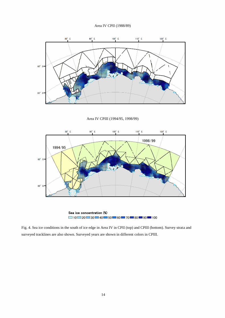
Sea ice conditions in the south of the ice edges in Area I, IV and western part of Area V were similar
between CPII and CPIII. However, extent of spatial distribution of large baleen whales was expanded in these
areas from CPII to CPIII (Murase et al., 2011). Environmental condition in Area I was also different between
CPII and CPIII. Number of Antarctic minke whales in the south of ice edge should be related to the multiple
factors. Region-specific integrated approach should be taken to estimate number of animals in the south of the
ice edge because factors affecting abundance estimate are different from region to region.
ACKNOWLEDGEMENT
The authors express their thanks to the crews and the researchers who engaged in the surveys to collect valuable
data. We thank IWC who provided partial funding for this study.
REFERENCES
Bjørgo, E., Johnannessen, O. M. and Miles, M. W. 1997. Analysis of merged SMMR-SMMI time series of Arctic and Antarctic sea ice parameters 1978-1995. Geophys. Res. Lett. 24: 413-416. Bromwich, D. H., Chen, B. and Hines, K. M. 1998. Global atmospheric impacts
induced by year-round open water adjacent to Antarctica. J. Geophys. Res. 103: 11173-11189.
Branch, T. A. 2005. Combining estimates from the third circumpolar set of surveys. J. Cetacean Res. Manage. 7 (suppl.): 231-233.
Branch, T. A. 2006. Abundance estimates for Antarctic minke whales from three completed circumpolar sets of survey, 1978/79 to 2003/04.
Paper SC/58/IA18, presented to the 58th IWC Scientific Committee, May 2006 (unpublished). 28pp.

3
Branch, T. A. and Butterworth, D. S. 2001. Southern Hemisphere minke whales: standardised abundance estimates from the 1978/79 to 1997/98 IDCR-SOWER surveys. J. Cetacean Res. Manage. 3: 143-174.
Burt, M. L. 2004. Overview of the standard dataset of IDCR/SOWER data. Paper SC/56/IA2 presented to the 56th IWC Scientific
Committee, June 2004 (unpublished). 3pp.
Comiso, J. 1999, updated 2008. Bootstrap Sea Ice Concentrations from NIMBUS-7 SMMR and DMSP SSM/I, [list dates you used]. Boulder,
Colorado USA: National Snow and Ice Data Center. Digital media.
Hanna, E.2001. Anomalous peak in Antarctic sea-ice area, winter 1998, coincident with EÑSO. Geophys. Res. Lett. 28: 1595-1598.
IWC 2002a. Report of the Scientific Committee. J. Cetacean Res. Manage. 4 (suppl.): 1-78.
IWC 2002b. Summary of factors (other than a real change in abundance) that might have contributed to the change in IDCR/SOWER abundance estimates. J. Cetacean Res. Manage. 4 (supp.): 248-268.
IWC 2003a. Report of the scientific committee, Annex G: Report of the sub-committee on the comprehensive assessment of whale stocks – in depth assessment. J. Cetacean Res. Manage. 5 (suppl.): 286-290.
IWC 2003. Hypotheses that may explain why the estimates of abundance for the third circumpolar set of survey (CP) using ‘the standard
methods’ are appreciably lower than estimates for the second CP. J. Cetacean Res. Manage. 5 (suppl.): 286-290.
IWC 2008. Report of the scientific committee, Annex G: Report of the sub-committee on in depth assessment (IA). J. Cetacean Res. Manage.
10 (suppl.): 167-181.
IWC. 2011. Report of the scientific committee. J. Cetacean Res. Manage. 12 (suppl.) (in press)
Matsuoka, K., Ensor, P., Hakamada, T., Shimada, H., Nishiwaki, S., Kasamatsu, F. and Kato, H. 2003. Overview of minke whale sightings
surveys conducted on IWC/IDCR SOWER Antarctic cruises from 1978/79 to 2000/01. J. Cetacean Res. Manage. 5: 173-201.
Murase, H. and Kitakado, T. 2010. Progress of preparation of sea ice data to investigate the relationship between sea ice characteristics and
Antarctic minke whale abundance estimates. Paper SC/61/IA4 presented to the 62nd IWC Scientific Committee, May 2010 (unpublished). 9pp.
Murase, H., Nishiwaki, S., Matsuoka, K., Hakamda, T. and Kitakado, T. 2011. Changes in baleen whale distribution patterns between CPII
and CPIII. Paper SC/63/IA11 presented to the 63rd IWC C Scientific Committee, May 2011 (unpublished).
Shimada, H., Segawa, K. and Murase, H. 2001. Tentative trial for estimation of Antarctic minke whale abundance within pack ice region
incorporating IDCR/SOWER data with meteorological satellites data. Paper SC/53/IA14 presented to the 52th IWC Scientific Committee, June 2000 (unpublished). 6pp.
Zwally, H. J., Comiso, J. C., Parkinson, C. L. and Cavalieri, D. J. 2002. Variability of Antarctic sea ice 1979-1998. J. Geophys. Res.
107(C5):10.1029/2000JC000733.
Table 1. Central meridians and latitude of origins used in the the South Pole Lambert azimuthal equal area
projection.
AreaCentral
meridians
latitude
of origins
I 90W 66S
II 30W 69S
III 35E 65S
IV 100E 65S
V 165E 69S
VI 145W 65S

4
Table 2. Start and end dates of survey used to calculate average sea ice concentrations.
Year Start End Year Start End Year Start End Year Start End
120W-115W 1990/2/8 1990/2/10 2001/1/31 2001/2/11 70E-75E 1989/1/12 1989/1/20 1995/2/11 1995/2/20
115W-110W 1990/2/5 1990/2/9 2001/2/7 2001/2/15 75E-80E 1989/1/10 1989/1/21 1995/2/13 1995/2/24
110W-105W 1990/1/31 1990/2/6 1994/1/4 1994/1/7 80E-85E 1989/1/8 1989/1/11 1999/1/20 1999/1/26
105W-100W 1990/1/24 1990/1/31 1994/1/6 1994/1/11 85E-90E 1989/1/2 1989/1/9 1999/1/23 1999/1/29
100W-95W 1990/1/22 1990/1/25 1994/1/9 1994/1/18 90E-95E 1988/12/31 1989/1/4 1999/1/26 1999/1/31
95W-90W 1990/1/16 1990/1/22 1994/1/15 1994/1/22 95E-100E 1988/12/29 1988/12/31 1999/1/28 1999/2/1
90W-85W 1990/1/14 1990/1/19 1994/1/18 1994/1/31 100E-105E 1989/1/25 1989/1/28 1999/2/1 1999/2/5
85W-80W 1990/1/12 1990/1/18 1994/1/25 1994/2/2 105E-110E 1989/1/27 1989/1/30 1999/2/3 1999/2/8
80W-75W 1990/1/7 1990/1/15 2000/1/15 2000/1/27 110E-115E 1989/1/29 1989/2/3 1999/2/5 1999/2/10
75W-70W 1990/1/4 1990/1/11 2000/1/17 2000/2/3 115E-120E 1989/2/1 1989/2/5 1999/2/10 1999/2/15
70W-65W 1989/12/30 1990/1/7 2000/2/1 2000/2/10 120E-125E 1989/2/5 1989/2/7 1999/2/15 1999/2/21
65W-60W 1989/12/29 1990/1/4 2000/2/7 2000/2/13 125E-130E 1989/2/8 1989/2/10 1999/2/17 1999/2/22
60W-55W 130E-135E 2001/12/27 2002/1/2
55W-50W 135E-140E 2002/1/1 2002/1/28
50W-45W 140E-145E 2002/1/6 2002/2/3
45W-40W 145E-150E 2002/1/23 2002/2/10
40W-35W 150E-155E 2003/1/29 2003/2/7
35W-30W 155E-160E 2003/2/5 2003/2/15
30W-25W 160E-165E 2003/2/18 2003/2/25
25W-20W165E-170E
(N of 71S)2002/12/23 2003/1/25
20W-15W165E-170E
(S of 71S)
15W-10W 170E-175E
10W-5W 175E-'180
5W-0 180-175W
0-5E 1988/1/23 1988/1/24 1992/12/26 1992/12/31 175W-170W
5E-10E 1988/1/19 1988/1/24 1992/12/31 1993/1/3 170W-165W
10E-15E 1988/1/18 1988/1/22 1993/1/3 1993/1/7 165W-160W
15E-20E 1988/1/15 1988/1/20 1993/1/6 1993/1/11 160W-155W
20E-25E 1988/1/11 1988/1/19 1993/1/11 1993/1/16 155W-150W
25E-30E 1988/1/9 1988/1/17 1993/1/17 1993/1/23 170W-165W 1991/1/3 1991/1/9 1996/1/13 1996/1/23
30E-35E 1993/1/20 1993/1/25 165W-160W 1991/1/7 1991/1/13 1996/1/20 1996/1/30
35E-40E 1993/1/24 1993/1/31 160W-155W 1991/1/12 1991/1/16 1996/1/27 1996/2/4
40E-45E 1995/1/14 1995/1/17 155W-150W 1991/1/14 1991/1/20 1996/2/4 1996/2/10
45E-50E 1995/1/16 1995/1/25 150W-145W 1991/1/19 1991/1/21 1996/2/10 1996/2/20
50E-55E 1995/1/25 1995/1/27 145W-140W 1991/1/23 1991/1/26 1996/2/20 1996/2/22
55E-60E 1995/1/27 1995/1/30 140W-135W 1991/1/26 1991/1/31 2001/1/16 2001/1/23
60E-65E 1995/2/4 1995/2/9 135W-130W 1991/1/31 1991/2/6 2001/1/22 2001/1/26
65E-70E 1995/2/7 1995/2/12 130W-125W 1991/2/6 1991/2/8 2001/1/24 2001/2/22
125W-120W 1991/2/9 1991/2/11 2001/1/28 2001/2/20
1985/12/26 1986/2/18
1986/12/29 1987/2/4
1998/1/20 1998/2/15
1997/1/16 1997/2/14
III
1992/93
1994/95
1987/88
IV
V
2000/01
1993/94
1999/00
1989/90I
II 1986/87
1997/98
1996/96
No sea ice data
CPII CPIIIArea Longitude
1988/89
Area LongitudeCPII CPIII
1990/91
2001/02
2002/03
2003/12/27 2004/2/82003/04
VI
1995/96
2000/01
1994/95
1998/99
1985/86

5
Table 3. Open sea ice area (km2) in the south of ice edge in each 5º longitudinal sector in Area I in CPII and CPIII.
120W-115W 115W-110W 110W-105W 105W-100W 100W-95W 95W-90W 90W-85W 85W-80W 80W-75W 75W-70W 70W-65W 65W-60W
0-5% 5,109 393 3,023 4,938 455 4,178 341 4,547 25,831 9,823 58,639
10-15% 792 809 1,613 1,121 404 2,756 64 2,109 1,893 11,561
15-20% 565 2,209 297 30 1,854 1,928 497 847 969 1,224 10,419
20-25% 1,411 750 697 689 348 1,165 493 1,156 126 649 44 7,530
25-30% 56 835 469 1,277 772 3,124 1,196 656 671 638 1,398 896 11,987
30-35% 452 616 1,039 443 1,224 2,863 607 20 644 50 7,959
35-40% 714 2,594 455 567 2,130 660 276 182 7,580
40-45% 1,009 220 1,010 3,400 1,523 1,010 532 537 2,791 55 904 12,992
45-50% 285 483 1,857 2,380 457 482 1,381 1,571 485 9,382
50-55% 896 1,331 1,687 2,138 439 2,945 1,042 3,278 251 14,008
5-10% 1,640 3,314 290 1,613 224 928 404 190 2,290 2,202 13,095
55-60% 351 1,130 1,399 1,045 402 1,163 1,887 2,538 2,206 528 120 12,769
60-65% 668 1,395 1,288 1,638 699 315 317 2,000 193 941 9,453
65-70% 586 577 1,285 1,143 310 862 302 1,727 1,349 240 3 8,384
70-75% 643 240 1,419 631 515 509 1,277 1,145 292 6,671
75-80% 222 499 969 1,033 408 374 620 610 375 330 88 5,530
80-85% 588 1,176 1,275 1,412 915 1,184 493 143 181 7,367
85-90% 210 219 988 1,515 304 307 428 823 533 79 31 5,437
90-95% 395 381 1,044 217 37 464 681 257 287 3,763
95-100% 382 465 335 117 518 944 607 3,367
Total 16,183 19,005 20,595 27,416 7,997 11,955 12,271 28,930 16,223 14,772 36,230 16,313 227,892
120W-115W 115W-110W 110W-105W 105W-100W 100W-95W 95W-90W 90W-85W 85W-80W 80W-75W 75W-70W 70W-65W 65W-60W
0-5% 2,680 7,424 10,290 457 564 11,368 1,126 1,375 6,252 16,307 8,675 66,518
10-15% 305 1,573 794 111 608 769 799 1,039 4,300 3,895 660 1,908 16,760
15-20% 843 1,217 752 842 799 909 1,776 1,470 1,490 1,931 523 12,550
20-25% 3,694 1,372 699 1,272 1,321 1,413 1,353 2,058 3,333 1,412 2,074 564 20,566
25-30% 1,084 1,777 1,294 47 275 1,312 3,912 1,998 2,604 585 37 14,926
30-35% 1,890 1,405 573 365 1,188 1,598 496 1,787 1,218 423 983 11,927
35-40% 2,317 1,694 581 2,276 956 407 3,799 1,988 559 607 347 15,530
40-45% 1,644 1,046 519 1,519 978 535 1,584 1,518 3,364 310 13,017
45-50% 1,966 986 927 959 1,292 1,395 3,753 2,724 2,375 336 184 16,898
50-55% 826 421 857 1,708 880 433 3,420 835 766 1,227 11,373
5-10% 818 1,674 1,684 1,134 661 2,461 1,706 353 5,030 3,786 1,610 20,918
55-60% 412 783 390 774 395 595 2,286 582 765 49 7,030
60-65% 976 665 1,028 1,093 1,337 2,405 3,723 1,216 650 564 13,657
65-70% 1,142 601 575 291 804 2,302 788 1,014 7,517
70-75% 505 729 242 260 736 502 986 953 676 463 6,052
75-80% 581 926 144 835 200 1,581 1,353 641 1,534 7,795
80-85% 706 139 1,120 429 167 319 779 822 610 181 5,271
85-90% 637 335 573 424 209 254 763 248 426 400 210 4,479
90-95% 361 507 455 169 79 219 784 237 166 131 3,109
95-100% 454 440 611 139 290 298 412 204 125 184 3,160
Total 23,840 25,711 22,033 15,564 8,969 23,217 19,542 36,571 27,811 31,111 29,851 14,833 279,053
CPIII (2000/2001) CPIII (1993/1994) CPIII (1999/2000)
TotalSea ice
concentration
Area I
TotalSea ice
concentration
CPII (1989/1990)
Area I

6
Table 4. Open sea ice area (km2) in the south of ice edge in each 5º longitudinal sector in Area II in CPII and CPIII.
60W-55W 55W-50W 50W-45W 45W-40W 40W-35W 35W-30W 30W-25W 25W-20W 20W-15W 15W-10W 10W-5W 5W-0
0-5% 2,509 89 38,262 53,609 83,137 5,571 9,443 10,860 9,636 2,392 215,509
10-15% 374 3,875 7,035 12,619 5,522 36,961 20,442 25,941 2,443 1,607 1,837 216 118,871
15-20% 178 3,864 6,692 10,422 5,205 23,053 11,801 27,732 2,290 2,054 2,139 1,072 96,502
20-25% 7,833 7,661 9,771 2,774 5,570 7,157 17,070 695 861 851 60,244
25-30% 653 5,646 4,584 7,867 3,918 3,282 17,247 18,272 1,754 387 629 3,289 67,527
30-35% 347 4,787 4,859 7,957 1,831 4,258 15,270 6,783 592 46,684
35-40% 3,104 4,272 5,637 7,905 3,374 2,821 16,675 493 549 1,636 46,467
40-45% 2,043 3,085 5,661 5,707 2,056 6,316 12,945 969 638 39,420
45-50% 756 2,815 6,107 4,317 2,823 9,205 9,887 803 1,309 38,020
50-55% 435 2,545 7,276 4,727 3,401 7,514 2,448 448 28,793
5-10% 1,077 3,701 9,159 12,501 19,955 7,649 22,628 5,751 2,102 419 836 85,779
55-60% 1,334 4,154 9,559 3,064 4,971 4,322 3,304 293 31,000
60-65% 371 2,689 11,871 4,063 3,053 4,693 1,324 326 106 28,496
65-70% 2,602 8,209 2,287 2,361 2,902 890 479 19,730
70-75% 737 2,692 4,215 1,693 1,246 3,246 202 14,031
75-80% 277 4,025 2,054 1,578 1,421 3,637 144 13,136
80-85% 63 2,450 1,790 1,243 1,382 1,708 8,635
85-90% 1,036 2,670 1,110 1,697 1,614 1,776 9,903
90-95% 1,008 2,850 2,046 1,012 1,778 591 9,284
95-100% 4,499 3,665 2,071 1,851 1,570 170 13,826
Total 20,801 70,309 145,860 155,889 153,390 135,245 151,462 112,901 18,920 10,330 6,302 10,450 991,859
60W-55W 55W-50W 50W-45W 45W-40W 40W-35W 35W-30W 30W-25W 25W-20W 20W-15W 15W-10W 10W-5W 5W-0
0-5% 70,462 70,724 79,248 31,040 53,098 37,533 66,167 5,884 2,712 5,238 5,011 1,776 428,891
10-15% 4,812 5,061 10,975 18,598 12,781 8,472 782 796 3,784 6,300 3,198 75,559
15-20% 761 5,884 8,136 25,384 12,573 4,826 57 2,177 2,995 1,243 5,218 1,388 70,642
20-25% 2,075 2,786 7,005 20,726 17,251 4,218 707 695 2,827 3,437 1,497 63,223
25-30% 1,302 3,892 9,120 26,064 7,164 3,879 662 3,233 2,405 3,148 60,871
30-35% 1,608 3,666 6,721 15,884 4,881 3,041 1,233 1,850 2,144 41,029
35-40% 565 2,299 5,115 11,874 8,491 1,704 1,128 2,823 1,086 2,871 543 38,500
40-45% 1,033 3,100 5,172 9,804 5,684 1,964 1,032 3,206 536 1,734 2,734 35,999
45-50% 925 3,834 2,859 8,911 5,223 1,848 1,425 1,391 743 1,106 28,266
50-55% 1,339 2,918 3,859 7,215 5,176 414 1,661 1,339 436 1,339 734 26,429
5-10% 5,074 8,160 15,675 19,454 15,969 13,548 4,421 2,465 413 6,585 2,407 1,669 95,840
55-60% 1,489 1,524 2,610 5,023 4,963 1,318 134 17,060
60-65% 2,218 4,665 1,683 4,988 2,711 41 2,367 340 788 19,801
65-70% 1,721 3,805 3,530 2,673 605 1,989 335 14,657
70-75% 1,435 2,626 3,935 3,747 737 649 639 13,767
75-80% 1,184 1,740 3,445 2,006 395 648 285 9,704
80-85% 294 1,749 3,439 1,722 26 581 7,811
85-90% 838 1,642 3,452 1,521 129 7,583
90-95% 818 1,681 2,256 1,495 458 119 6,827
95-100% 1,993 2,801 2,055 644 348 18 7,859
Total 101,946 134,557 180,290 218,773 158,507 82,300 71,428 26,839 24,781 25,658 28,497 16,740 1,070,316
Sea ice
concentration
Sea ice
concentration
Area II
CPII (1986/1987) Total
Area II
TotalCPIII (1997/1998) CPIII (1996/1997)

7
Table 5. Open sea ice area (km2) in the south of ice edge in each 5º longitudinal sector in Area III in CPII and CPIII. Note that satellite sea ice data were not available between 30ºE
and 70ºE in CPII.
0-5E 5E-10E 10E-15E 15E-20E 20E-25E 25E-30E 30E-35E 35E-40E 40E-45E 45E-50E 50E-55E 55E-60E 60E-65E 65E-70E
0-5% 2,326 3,583 1,954 4,357 15,631 747 28,597
10-15% 356 777 796 1,575 1,997 5,501
15-20% 230 738 614 1,491 1,533 4,606
20-25% 189 1,545 1,390 703 2,695 6,523
25-30% 1,238 7 2,182 153 3,580
30-35% 617 630 1,232 1,185 3,664
35-40% 1,133 1,127 583 2,844
40-45% 1,519 456 511 1,034 3,520
45-50% 90 682 940 1,712
50-55% 459 389 867 422 2,137
5-10% 888 1,821 2,171 3,152 8,032
55-60% 1 370 984 1,355
60-65% 301 339 581 710 1,930
65-70% 75 121 904 1,101
70-75% 20 686 706
75-80% 280 165 445
80-85% 22 22
85-90% 0
90-95% 0
95-100% 0
Total 2,326 5,246 12,192 11,244 30,507 14,761 76,275
0-5E 5E-10E 10E-15E 15E-20E 20E-25E 25E-30E 30E-35E 35E-40E 40E-45E 45E-50E 50E-55E 55E-60E 60E-65E 65E-70E
0-5% 79,383 51,330 48,454 1,828 2,119 5,841 5,528 2,007 6,954 9,223 212,667
10-15% 3,202 2,364 797 2,102 74 3,908 989 33 125 802 3,909 18,306
15-20% 3,659 1,475 1,465 1,865 1,116 759 1,537 367 1,822 14,064
20-25% 2,978 693 1,394 1,408 711 691 690 1,406 34 581 2,470 13,057
25-30% 354 2,610 1,306 2,028 650 2,060 1,083 722 1,266 1,427 13,505
30-35% 1,800 602 893 1,658 1,226 603 534 2,698 10,013
35-40% 958 1,678 1,098 432 3,310 562 830 8,868
40-45% 1,422 1,006 1,043 1,895 1,315 945 518 847 1 8,992
45-50% 2,781 463 1,409 849 2,122 456 757 460 1,357 490 11,144
50-55% 1,587 440 406 1,166 2,637 872 412 338 256 667 1,078 9,860
5-10% 8,057 4,148 3,309 1,125 1,151 181 2,216 1,856 99 1,397 1,741 25,279
55-60% 1,344 747 1,143 276 2,255 217 1,164 192 8 392 771 8,509
60-65% 1,798 959 325 2,325 679 326 49 1,757 357 8,576
65-70% 1,392 1,511 312 851 2,250 364 376 1,289 8,343
70-75% 957 2,719 246 1,041 2,196 233 260 250 383 233 466 8,985
75-80% 639 208 1,278 1,581 182 224 278 359 641 607 5,997
80-85% 137 350 799 479 335 349 467 89 6 164 870 4,045
85-90% 220 476 217 132 133 370 122 101 18 147 1,936
90-95% 75 549 464 44 207 56 326 10 144 261 2,136
95-100% 179 337 385 155 28 158 42 1,283
Total 98,592 77,379 66,033 12,682 16,666 19,988 25,097 18,314 2,975 1,846 7,227 7,133 17,022 24,611 395,566
CPII (1987/1988)
Area III
TotalSea ice
concentration
Area III
TotalSea ice
concentrationCPIII (1992/1993) CPIII (1994/1995)
NA

8
Table 6. Open sea ice area (km2) in the south of ice edge in each 5º longitudinal sector in Area IV in CPII and CPIII.
70E-75E 75E-80E 80E-85E 85E-90E 90E-95E 95E-100E 100E-105E 105E-110E 110E-115E 115E-120E 120E-125E 125E-130E
0-5% 7,880 18,949 14,850 3,809 7,291 365 869 54,014
10-15% 2,346 2,278 6,194 807 3,109 2,733 47 17,514
15-20% 1,455 3,208 268 2,352 2,051 9,335
20-25% 437 4,779 3,304 2,150 1,445 1,282 1,279 14,676
25-30% 465 829 662 3,218 1,277 1,978 1,239 636 10,304
30-35% 1,832 1,832 13 2,239 621 1,209 7,746
35-40% 650 1,594 181 3,935 1,333 523 1,016 1,067 1,141 319 11,758
40-45% 2,590 1,707 1,058 506 2,112 511 356 169 1,217 1,020 555 11,802
45-50% 438 3,840 1,552 755 470 632 471 1,408 910 924 465 11,867
50-55% 924 2,098 1,327 277 844 870 1,709 442 847 1,180 998 1,214 12,730
5-10% 1,010 3,319 11,588 1,925 5,163 1,775 1,033 25,812
55-60% 1,381 1,367 564 396 2,780 580 782 1,501 1,172 10,524
60-65% 915 504 1,549 358 356 678 95 1,000 978 344 6,778
65-70% 271 306 1,434 396 72 1,555 1,273 235 100 1,492 1,044 8,178
70-75% 1,935 1,113 1,148 1,313 887 508 849 502 17 8,271
75-80% 207 812 630 186 189 619 147 858 849 40 4,539
80-85% 356 915 82 736 307 136 578 1,001 945 5,056
85-90% 236 27 726 179 87 1,359 320 214 644 130 363 4,284
90-95% 101 518 58 3 908 60 126 274 946 2,994
95-100% 348 204 220 44 125 237 216 1,394
Total 25,430 45,270 13,576 5,426 51,849 16,745 7,988 19,962 20,362 14,589 11,613 6,765 239,575
70E-75E 75E-80E 80E-85E 85E-90E 90E-95E 95E-100E 100E-105E 105E-110E 110E-115E 115E-120E 120E-125E 125E-130E
0-5% 50 57 186 0 78 4 5 2 381
10-15% 161 263 121 491 74 326 133 1,569
15-20% 59 499 94 147 150 14 24 449 1,435
20-25% 1,171 187 405 173 373 179 137 128 42 616 430 3,840
25-30% 335 116 380 228 920 617 899 505 4,001
30-35% 5 903 313 582 898 307 199 3,207
35-40% 673 1,771 330 852 229 158 633 8 4,654
40-45% 1,063 320 763 364 355 1,231 754 816 5,667
45-50% 1,215 1,293 397 426 1,396 1,334 438 6,500
50-55% 1,613 1,925 1,934 461 3,089 1,401 1,616 911 460 934 14,343
5-10% 122 122 350 125 90 101 68 58 27 1,063
55-60% 1,572 1,543 675 510 2,070 2,509 535 2,951 804 13,170
60-65% 1,116 1,593 558 373 723 2,354 1,752 1,654 560 1,693 12,376
65-70% 1,838 597 1,413 594 2,434 628 4,359 341 1,218 640 14,061
70-75% 1,285 1,348 1,536 1,958 1,941 1,636 1,334 1,981 2,810 15,829
75-80% 2,767 676 1,388 5,701 1,358 1,686 949 2,509 2,004 712 19,749
80-85% 1,520 753 1,444 4,256 4,524 2,066 742 6,397 1,382 1,507 24,591
85-90% 3,604 788 202 3,952 1,505 2,415 3,196 2,571 4,924 23,158
90-95% 4,947 1,671 3,623 3,332 1,314 2,918 1,630 6,182 3,314 28,931
95-100% 8,862 9,506 4,634 27,251 7,048 16,012 3,187 24,652 101,151
Total 1,904 365 34,124 19,583 23,937 49,142 26,665 33,372 23,722 49,194 18,142 19,527 299,676
Total
Total
Area IV
CPII (1988/1989)Sea ice
concentration
Sea ice
concentrationCPIII (1994/1995) CPIII (1998/1999)
Area IV

9
Table 7. Open sea ice area (km2) in the south of ice edge in each 5º longitudinal sector in Area V in CPII and CPIII.
130E-135E 135E-140E 140E-145E 145E-150E 150E-155E 155E-160E 160E-165E 165E-170E 170E-175E 175E-180 180-175W 175W-170W 170W-165W 165W-160W 160W-155W 155W-150W
0-5% 2,944 14,786 245 5,330 503 5,316 21,347 1,710 1,419 320 332 1 5,208 3,250 62,711
10-15% 3,158 1,497 1,542 77 2,479 2,361 984 417 335 1,226 4,146 18,223
15-20% 8,321 235 1,012 1,358 1,508 2,221 5,541 259 759 2,432 23,646
20-25% 779 1,275 2,846 667 931 5,452 304 831 2,083 15,168
25-30% 603 325 769 1,334 1,302 3,351 1,940 2,120 1,242 9,486 10,321 32,794
30-35% 30 235 1,161 1,246 1,636 5,659 402 3,025 898 4,580 14,186 33,058
35-40% 235 19 1,435 1,688 1,486 1,084 51 3,970 1,888 489 8,617 9,892 30,854
40-45% 745 521 954 3,196 46 3,204 3,741 1,164 2,396 3,073 19,041
45-50% 35 454 952 985 2,986 2,050 1,391 2,091 5,683 3,013 19,641
50-55% 425 1,725 601 2,815 1,324 2,146 1,942 6,364 3,416 20,757
5-10% 9,035 4,063 504 1,594 1,354 7,717 1,071 1,149 2,601 29,089
55-60% 87 558 149 2,447 1,554 2,998 2,748 772 2,774 6,143 3,938 24,167
60-65% 28 809 1,006 1,436 675 326 2,343 1,625 8,060 6,084 22,392
65-70% 211 1,605 1,480 2,129 1,569 578 2,910 2,355 11,674 24,511
70-75% 340 2,230 1,150 1,433 1,909 2,102 3,646 736 13,546
75-80% 22 406 1,286 1,974 224 3,908 2,554 1,387 1,232 12,991
80-85% 874 798 3,907 2,843 995 476 9,894
85-90% 122 3,574 475 2,165 3,441 498 10,276
90-95% 12 734 252 998
95-100%
Total 25,075 20,347 1,183 15,518 7,318 24,730 54,707 44,050 4,435 320 332 21,296 29,016 32,669 74,722 68,041 423,757
130E-135E 135E-140E 140E-145E 145E-150E 150E-155E 155E-160E 160E-165E 165E-170E 170E-175E 175E-180 180-175W 175W-170W 170W-165W 165W-160W 160W-155W 155W-150W
0-5% 33,408 2,058 1,650 938 6,621 2,116 21,866 538 1,092 44,341 50,150 38,311 42,493 245,581
10-15% 3,288 56 1,159 2,382 2,625 1,193 245 783 2,349 3,874 765 1,828 20,547
15-20% 730 832 1,505 1,535 740 741 2,626 1,190 732 2,549 750 13,930
20-25% 362 646 5 652 81 713 887 3,372 3,912 3,259 1,386 1,403 682 715 18,076
25-30% 670 1,165 642 2,508 1,379 3,277 1,238 795 1,215 1,330 661 1,911 16,792
30-35% 1,584 302 213 196 251 3,139 2,045 1,844 765 1,792 33 69 1,193 13,426
35-40% 580 613 94 1,266 3,244 1,635 3,832 2,947 1,139 2,804 1,132 616 3,369 23,270
40-45% 383 1,017 804 182 1,123 3,882 2,089 6,634 2,089 1,037 514 2,050 3,839 25,642
45-50% 61 4 435 1,448 3,006 35 479 4,223 1,432 934 2,353 3,922 1,863 20,193
50-55% 39 421 63 590 3,377 42 5,599 423 2,143 1,718 2,660 2,529 19,603
5-10% 2,479 721 176 911 5,535 290 3,456 16 5,640 2,046 851 22,119
55-60% 326 764 371 1,539 1,125 2,714 2,102 1,911 2,983 4,735 765 19,334
60-65% 346 692 657 1,498 1,335 3,469 2,724 3,679 6,030 8,623 2,345 31,398
65-70% 220 307 272 20 1,086 2,258 42 2,652 3,169 7,641 6,695 6,725 2,053 33,140
70-75% 97 228 255 231 1,517 528 262 7,911 5,018 4,315 5,169 3,990 29,519
75-80% 5 216 435 334 115 808 1,066 1,652 2,895 2,198 1,918 4,036 15,678
80-85% 490 272 72 1,269 674 172 347 515 2,557 6,368
85-90% 260 373 30 714 325 897 171 1,062 3,833
90-95% 351 59 655 802 312 773 2 2,955
95-100% 182 734 566 369 710 2,561
Total 44,033 9,786 1,925 11,219 2,809 2,486 34,011 33,061 28,432 16,372 38,365 30,540 84,956 87,855 80,821 77,299 583,968
Sea ice
concentration
Sea ice
concentration
Area V
CPII (1985/1986) Total
Area V
TotalCPIII (2001/2002) CPIII (2002/2003) CPIII (2003/2004)
10
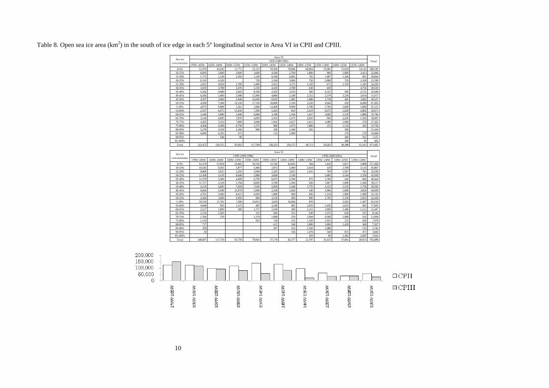
Table 8. Open sea ice area (km2) in the south of ice edge in each 5º longitudinal sector in Area VI in CPII and CPIII.
170W-165W 165W-160W 160W-155W 155W-150W 150W-145W 145W-140W 140W-135W 135W-130W 130W-125W 125W-120W
0-5% 51,979 42,042 11,771 22,125 59,560 78,686 68,964 23,982 15,039 14,142 388,290
10-15% 6,093 3,600 3,600 3,600 4,500 2,700 1,800 900 1,800 3,413 32,006
15-20% 1,775 1,530 2,295 1,530 9,180 6,885 765 1,997 1,206 901 28,064
20-25% 6,310 4,320 720 2,160 3,600 720 2,880 720 2,160 23,590
25-30% 2,025 4,050 2,700 5,400 2,025 3,375 1,350 675 1,350 1,343 24,293
30-35% 3,910 3,780 3,476 3,150 4,410 3,780 630 630 4,754 28,520
35-40% 5,202 4,680 2,925 8,190 2,925 3,510 585 4,315 585 2,731 35,649
40-45% 6,436 5,400 5,940 12,960 4,860 3,240 2,552 2,578 3,236 3,814 51,017
45-50% 4,507 3,960 5,940 16,830 8,910 1,485 1,980 1,738 495 3,682 49,527
50-55% 4,500 7,200 12,150 17,550 10,800 1,350 2,250 4,944 450 6,009 67,203
5-10% 4,073 9,888 1,261 1,800 14,400 9,900 2,700 2,700 3,600 1,800 52,122
55-60% 2,107 6,075 13,450 7,290 5,423 810 2,419 6,075 1,620 4,802 50,071
60-65% 3,240 2,880 5,040 6,840 3,180 2,160 1,457 3,600 2,520 2,880 33,796
65-70% 3,140 4,095 7,870 4,095 2,554 1,675 2,835 945 2,205 1,583 30,997
70-75% 4,285 3,510 7,809 3,048 1,942 2,627 1,615 1,080 1,080 270 27,265
75-80% 4,568 4,500 6,750 1,575 900 1,973 1,800 225 1,124 342 23,756
80-85% 5,278 4,320 2,160 896 360 1,440 291 360 15,104
85-90% 4,046 4,185 675 135 1,080 278 270 10,668
90-95% 540 90 360 161 1,151
95-100% 360 45 405
Total 123,472 120,555 95,902 117,599 138,223 130,275 94,713 59,263 38,388 55,101 973,491
170W-165W 165W-160W 160W-155W 155W-150W 150W-145W 145W-140W 140W-135W 135W-130W 130W-125W 125W-120W
0-5% 52,370 57,818 23,405 18,742 12,742 42,825 184 1,416 5,057 2,899 217,458
10-15% 10,182 9,455 3,977 5,400 2,872 5,400 2,619 129 2,700 3,133 45,867
15-20% 8,866 3,825 2,295 3,060 2,295 3,825 1,431 769 5,507 765 32,639
20-25% 12,458 4,320 8,640 2,880 3,600 2,160 3,485 3,164 2,350 43,058
25-30% 11,570 5,400 4,409 6,750 6,075 2,700 675 1,760 242 842 40,424
30-35% 11,757 2,520 5,794 8,820 3,780 1,260 630 1,807 1,890 1,260 39,517
35-40% 4,233 4,095 7,020 7,020 5,850 2,340 1,755 3,225 2,102 1,756 39,395
40-45% 6,664 5,940 15,079 5,940 2,160 1,620 540 1,966 1,080 3,850 44,839
45-50% 4,781 3,960 8,415 4,950 1,980 990 856 2,234 1,980 1,980 32,126
50-55% 2,420 3,600 4,950 900 3,150 450 900 1,795 1,350 2,925 22,439
5-10% 10,310 11,701 7,200 10,813 3,650 16,004 870 3,595 1,367 65,510
55-60% 4,648 810 1,215 405 3,240 405 2,025 2,430 2,023 405 17,605
60-65% 2,527 1,800 360 1,737 2,160 360 2,151 1,800 1,440 1,112 15,447
65-70% 1,214 2,205 315 945 315 630 1,575 630 315 8,144
70-75% 1,764 270 1,179 1,080 270 1,094 4,590 1,080 532 11,858
75-80% 1,150 933 720 225 1,350 2,925 225 450 7,978
80-85% 717 612 540 1,800 1,800 1,439 360 7,267
85-90% 359 267 552 1,350 1,080 135 3,742
90-95% 20 336 1,478 540 815 471 3,660
95-100% 458 90 1,362 2,005 3,916
Total 148,007 117,719 92,759 79,843 57,178 82,577 22,797 35,415 37,681 28,913 702,889
Area VI
CPII (1990/1991)Sea ice
concentrationTotal
Sea ice
concentrationCPIII (1995/1996) CPIII (2000/2001)
Area VI
Total

11
Area I CPII (1989/90)
Area I CPIII (1993/94, 1999/00, 2000/01)
Sea ice concentration (%)
10 20 30 40 50 60 70 80 90 100
Fig. 1. Sea ice conditions in the south of ice edge in Area I in CPII (top) and CPIII (bottom). Survey strata and surveyed
tracklines are also shown. Surveyed years are shown in different colors in CPIII.

12
Area II CPII (1986/87)
Area II CPIII (1996/97, 1997/98)
Sea ice concentration (%)
10 20 30 40 50 60 70 80 90 100
Fig. 2. Sea ice conditions in the south of ice edge in Area II in CPII (top) and CPIII (bottom). Survey strata and
surveyed tracklines are also shown. Surveyed years are shown in different colors in CPIII.

13
Area III CPII (1987/88)
Area III CPIII (1992/93, 1994/95)
Sea ice concentration (%)
10 20 30 40 50 60 70 80 90 100
Fig. 3. Sea ice conditions in the south of ice edge in Area III in CPII (top) and CPIII (bottom). Survey strata and
surveyed tracklines are also shown. Surveyed years are shown in different colors in CPIII. Note that satellite sea ice
data were not available between 30ºE and 70ºE in CPII (purple area in the top).
14
Area IV CPII (1988/89)
Area IV CPIII (1994/95, 1998/99)
Sea ice concentration (%)
10 20 30 40 50 60 70 80 90 100
Fig. 4. Sea ice conditions in the south of ice edge in Area IV in CPII (top) and CPIII (bottom). Survey strata and
surveyed tracklines are also shown. Surveyed years are shown in different colors in CPIII.

15
Area V CPII (1985/86)
Area V CPIII (2001/02, 2002/03, 2003/04)
Sea ice concentration (%)
10 20 30 40 50 60 70 80 90 100
Fig. 5. Sea ice conditions in the south of ice edge in Area V in CPII (top) and CPIII (bottom). Survey strata and
surveyed tracklines are also shown. Surveyed years are shown in different colors in CPIII.

16
Area VI CPII (1990/91)
Aera VI CPIII (1995/96, 2000/01)
Sea ice concentration (%)
10 20 30 40 50 60 70 80 90 100
Fig. 6. Sea ice conditions in the south of ice edge in Area VI in CPII (top) and CPIII (bottom). Survey strata and
surveyed tracklines are also shown. Surveyed years are shown in different colors in CPIII.
Related Documents


