Open Motion Planning Library: A Primer - OMPLompl.kavrakilab.org/OMPL_Primer.pdf · Open Motion Planning Library: A Primer Kavraki Lab Rice University ompl.kavrakilab.org November

Open Motion Planning Library:A Primer

Kavraki LabRice University

ompl.kavrakilab.org

June 25, 2018

Contents

1 Introduction 11.1 Prerequisites for Using OMPL . . . . . . . . . . . . . . . . . . . . . . . . . . . . 1

2 Introduction to Sampling-based Motion Planning 22.1 Historical Notes . . . . . . . . . . . . . . . . . . . . . . . . . . . . . . . . . . . . 22.2 Sampling-based Motion Planning . . . . . . . . . . . . . . . . . . . . . . . . . . . 3

2.2.1 Problem Statement and Definitions . . . . . . . . . . . . . . . . . . . . . 42.2.2 Probabilistic Roadmap . . . . . . . . . . . . . . . . . . . . . . . . . . . . 42.2.3 Tree-based Planners . . . . . . . . . . . . . . . . . . . . . . . . . . . . . 62.2.4 Primitives of Sampling-based Planning . . . . . . . . . . . . . . . . . . . 8

3 Getting Started with OMPL.app 93.1 Using OMPL.app . . . . . . . . . . . . . . . . . . . . . . . . . . . . . . . . . . . 9

3.1.1 Selecting a Robot and an Environment . . . . . . . . . . . . . . . . . . . . 103.1.2 Choosing a Planner . . . . . . . . . . . . . . . . . . . . . . . . . . . . . . 113.1.3 Bounding the Environment . . . . . . . . . . . . . . . . . . . . . . . . . . 123.1.4 Saving and Replaying Solution Paths . . . . . . . . . . . . . . . . . . . . 12

3.2 OMPL.app vs. OMPL . . . . . . . . . . . . . . . . . . . . . . . . . . . . . . . . . 12

4 Planning with OMPL 134.1 Design Considerations . . . . . . . . . . . . . . . . . . . . . . . . . . . . . . . . 134.2 OMPL Foundations . . . . . . . . . . . . . . . . . . . . . . . . . . . . . . . . . . 144.3 Solving a Query . . . . . . . . . . . . . . . . . . . . . . . . . . . . . . . . . . . . 154.4 Compiling Code with OMPL . . . . . . . . . . . . . . . . . . . . . . . . . . . . . 164.5 Benchmarking . . . . . . . . . . . . . . . . . . . . . . . . . . . . . . . . . . . . . 17

5 Advanced Topics in OMPL 195.1 State Space Construction . . . . . . . . . . . . . . . . . . . . . . . . . . . . . . . 195.2 Planner Customization . . . . . . . . . . . . . . . . . . . . . . . . . . . . . . . . 195.3 Python Bindings . . . . . . . . . . . . . . . . . . . . . . . . . . . . . . . . . . . . 20

i

Chapter 1

Introduction

This document explains how the Open Motion Planning Library (OMPL) implements the basicprimitives of sampling-based motion planning, what planners are already available in OMPL, andhow to use the library to build new planners. This primer is segmented into the following sections:An introduction to sampling-based motion planning, a guide to setup OMPL for solving motionplanning queries using OMPL.app, a description of the motion planning primitives in OMPL todevelop your own planner, and an explanation of some advanced OMPL topics.

At the end of this document, users should be able to use OMPL.app to solve motion planningqueries in 2D and 3D workspaces, and utilize the OMPL framework to develop their own algo-rithms for state sampling, collision checking, nearest neighbor searching, and other components ofsampling-based methods to build a new planner.

1.1 Prerequisites for Using OMPLThis primer assumes that users are familiar with C++ programming and compiling code in a Unixenvironment. Additionally, users should have basic knowledge of sampling-based motion planning.OMPL and OMPL.app should also be installed. For information regarding the installation process,please see ompl.kavrakilab.org.

1

Chapter 2

Introduction to Sampling-based MotionPlanning

To put OMPL in context, a short introduction to the principles of sampling-based motion planningis first given. Robotic motion planning seeks to find a solution to the problem of “Go from thestart to the goal while respecting all of the robot’s constraints." From a computational point ofview, however, such an inquiry can be very difficult when the robot has a large number of degreesof freedom. For simplicity, consider the classical motion planning problem known as the pianomover’s problem. In this formulation, there exists a rigid object in 3D (the piano), as well as a setof known obstacles. The goal of the piano mover’s problem is to find a collision-free path for thepiano that begins at its starting position and ends at a prescribed goal configuration. Computing theexact solution to this problem is very difficult. In this setup, the piano has six degrees of freedom:three for movement in the coordinate planes (x,y,z), and three more to represent rotation along theaxes of these coordinate planes (roll, pitch, yaw). To solve the piano mover’s problem we mustcompute a set of continuous changes in all six of these values in order to navigate the piano fromits starting configuration to the goal configuration while avoiding obstacles in the environment. Ithas been shown that finding a solution for the piano mover’s problem is PSPACE-hard, indicatingcomputational intractability in the degrees of freedom of the robot [1, 2, 3].

2.1 Historical NotesOMPL specializes in sampling-based motion planning, which is presented in Section 2.2. Toput sampling-based methods in context, a very brief historical overview to the methods that havebeen proposed for motion planning is presented. Most of these methods were developed beforesampling-based planning, but are still applicable in many scenarios.

Exact and Approximate Cell Decomposition In some instances, it is possible to partition theworkspace into discrete cells corresponding to the obstacle free portion of the environment. Thisdecomposition can then be modeled as a graph (roadmap), where the vertices represent the individual

2

Chapter 2. Introduction to Sampling-based Motion Planning

cells and edges indicate adjacency among the cells. Utilizing this graph, the problem of moving apoint robot becomes a classical search from the cell with the starting position to the cell containingthe goal position. Such a formulation also works well in “controllable” systems (e.g., omni-directional base). There are cases though, for example when the robot has complex non-lineardynamics, where it is not clear how to move the system from one cell to an adjacent cell. It shouldalso be noted that the motion of robots are computed in states spaces that are high-dimensional.Partitioning these spaces into free (or approximately free) cells is difficult and impractical in mostcases.

Control-based Methods Control-based methods attempt to model the equations of motion ofthe system and apply ideas from control theory in order to navigate a system along a specifiedtrajectory. These approaches operate in the continuous space, and typically employ a feedback loopin order to effectively maneuver the system with minimal error. Using a control-based approachto navigate a robot is very fast and can be done in an online manner, which is necessary in manyapplications. Computing a desirable and feasible trajectory can be very difficult, however, in systemswith complex dynamics and/or cluttered environments, which heavily restrict the valid motions.

Potential Fields Conceptually, potential fields are a simple and intuitive idea. The classicalpotential field involves computing a vector at each point in the workspace by calculating the sum ofan attractive force emanating from the goal, and a repulsive force from all of the obstacles. Thepoint robot can then navigate using gradient descent to follow the potentials to the goal. Potentialfields have been generalized to systems with a rigid body by considering multiple points on therobot, and can operate in real-time. Navigating a system using a potential field, however, can faildue to local minima in the field itself, which stem from the heuristic combination of the forces inthe workspace. Ideally the field would be constructed in the state space of the system, but this isequivalent to solving the original problem. Some approaches consider a navigation function wherethe potential field is guaranteed to have a single minimum, but computing such a function is possibleonly in low-dimensional spaces and is non-trivial.

Randomized Planning Randomization in otherwise deterministic planners has shown to be veryeffective. In potential fields, for example, Brownian motions in which a random action is appliedfor a specific amount of time have been shown to be highly effective in guiding a system out of alocal minima. Randomized methods have also been applied to non-holonomic systems, particularlyin the field of sampling-based planning. Sampling-based methods were inspired by randomization,and the use of samples, random or deterministic, when planning are particularly effective for highdegree of freedom systems or those with complex dynamics.

2.2 Sampling-based Motion PlanningSampling-based motion planning is a powerful concept that employs sampling of the state space ofthe robot in order to quickly and effectively answer planning queries, especially for systems with

Open Motion Planning Library : A Primer ‖ 3


differential constraints or those with many degrees of freedom. Traditional approaches to solvingthese particular problems may take a very long time due to motion constraints or the size of thestate space. Sampling arises out of the need to quickly cover a potentially large and complex statespace to connect a start and goal configuration along a feasible and valid path.

The need to reason over the entire continuous state space causes traditional approaches tobreakdown in high-dimensional spaces. In contrast, sampling-based motion planning reasonsover a finite set of configurations in the state space. The sampling process itself computes in thesimplest case a generally uniform set of random robot configurations, and connects these samplesvia collision free paths that respect the motion constraints of the robot to answer the query. Mostsampling-based methods provide probabilistic completeness. This means that if a solution exists,the probability of finding a solution converges to one as the number of samples reasoned overincreases to infinity. Sampling-based approaches cannot recognize a problem with no solution.

2.2.1 Problem Statement and DefinitionsThis section will present the problem to be solved by the motion query using a sampling-basedmethod, and define some useful terminology that will be used throughout the remainder of theprimer.

Workspace: The physical space that the robot operates in. It is assumed that the boundary of theworkspace represents an obstacle for the robot.

State space: The parameter space for the robot. This space represents all possible configurationsof the robot in the workspace. A single point in the state space is a state.

Free state space: A subset of the state space in which each state corresponds to an obstacle freeconfiguration of the robot embedded in the workspace.

Path: A continuous mapping of states in the state space. A path is collision free if each element ofthe path is an element of the free state space.

From these definitions, the goal of a sampling-based motion planning query can be formalizedas the task of finding a collision path in the state space of the robot from a distinct start state to aspecific goal state, utilizing a path composed of configurations connected by collision free paths.

The remainder of this section will discuss two types of sampling-based planners, from whichmany of the state-of-the-art techniques can be derived from. It should be noted that many samplingstrategies exists, but their presentation is beyond the scope of this Primer.

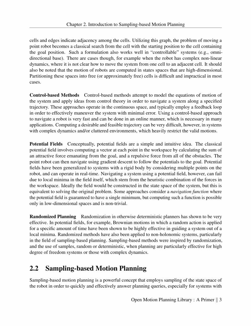
2.2.2 Probabilistic RoadmapThe probabilistic roadmap (PRM) is among the first sampling-based motion planners [4]. Thisapproach utilizes random sampling of the state space to build a roadmap of the free state space.This roadmap is analogous to a street map of a city. To illustrate the fundamentals of the PRM, asimple example of a 2D workspace and freely moving point robot will be used.



Figure 2.1: The 2D workspace and a single state for the point robot.

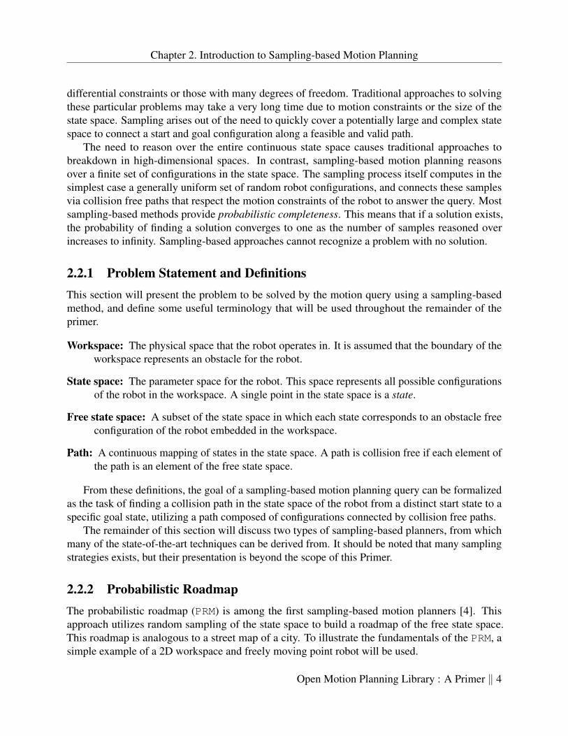
Consider the workspace in Figure 2.1. This image shows a bounded workspace for the pointrobot in which the shaded regions are obstacles. One particular state for the robot is highlighted.The PRM works by uniformly sampling the free state space and making connections between thesamples to form a roadmap of the free state space. The roadmap can be stored efficiently as a graphdata structure where the random samples compose the vertices, as in Figure 2.2. It should be notedthat the free state space is almost never explicitly known in sampling-based methods. Each samplethat is generated is checked for collision, and only collision free samples are retained. Additionally,there are many different ways to sample the free state space, and changing the sampling strategy isbeneficial in many planning instances.

Figure 2.2: One possible set of uniform random samples of the free state space

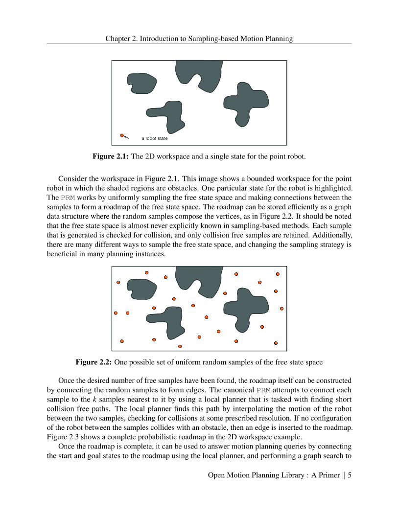
Once the desired number of free samples have been found, the roadmap itself can be constructedby connecting the random samples to form edges. The canonical PRM attempts to connect eachsample to the k samples nearest to it by using a local planner that is tasked with finding shortcollision free paths. The local planner finds this path by interpolating the motion of the robotbetween the two samples, checking for collisions at some prescribed resolution. If no configurationof the robot between the samples collides with an obstacle, then an edge is inserted to the roadmap.Figure 2.3 shows a complete probabilistic roadmap in the 2D workspace example.

Once the roadmap is complete, it can be used to answer motion planning queries by connectingthe start and goal states to the roadmap using the local planner, and performing a graph search to



Figure 2.3: Using a local planner, the PRM is formed by connecting samples that are close to oneanother using a straight path in the free state space.

find the shortest path in the roadmap. This is seen in Figure 2.4.

Figure 2.4: An example of a motion planning query on a PRM. The start and the goal are connectedto the roadmap, and the shortest path in the graph is found.

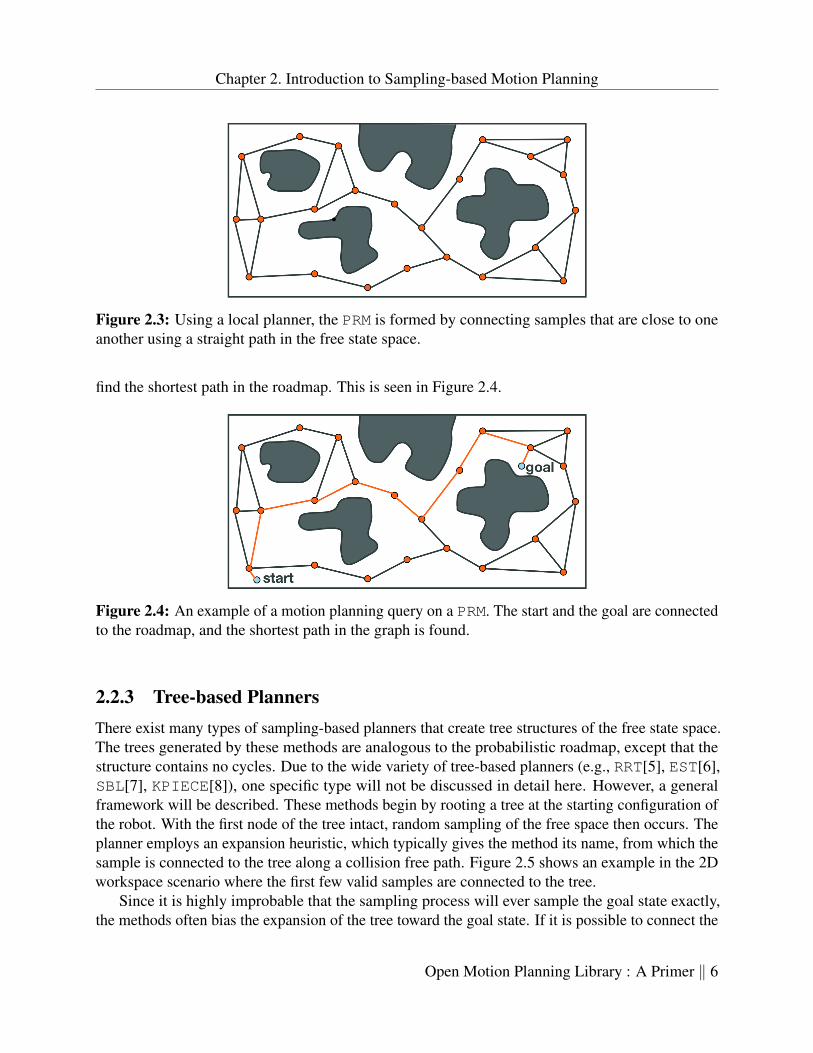
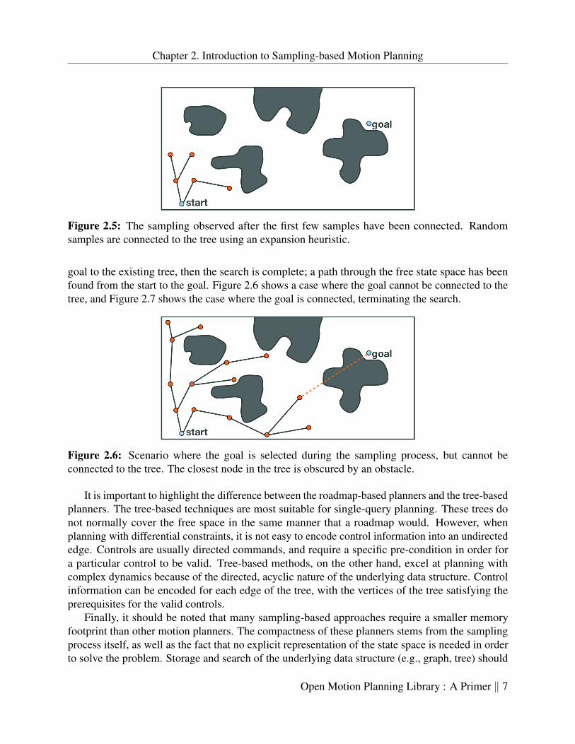
2.2.3 Tree-based PlannersThere exist many types of sampling-based planners that create tree structures of the free state space.The trees generated by these methods are analogous to the probabilistic roadmap, except that thestructure contains no cycles. Due to the wide variety of tree-based planners (e.g., RRT[5], EST[6],SBL[7], KPIECE[8]), one specific type will not be discussed in detail here. However, a generalframework will be described. These methods begin by rooting a tree at the starting configuration ofthe robot. With the first node of the tree intact, random sampling of the free space then occurs. Theplanner employs an expansion heuristic, which typically gives the method its name, from which thesample is connected to the tree along a collision free path. Figure 2.5 shows an example in the 2Dworkspace scenario where the first few valid samples are connected to the tree.

Since it is highly improbable that the sampling process will ever sample the goal state exactly,the methods often bias the expansion of the tree toward the goal state. If it is possible to connect the



Figure 2.5: The sampling observed after the first few samples have been connected. Randomsamples are connected to the tree using an expansion heuristic.

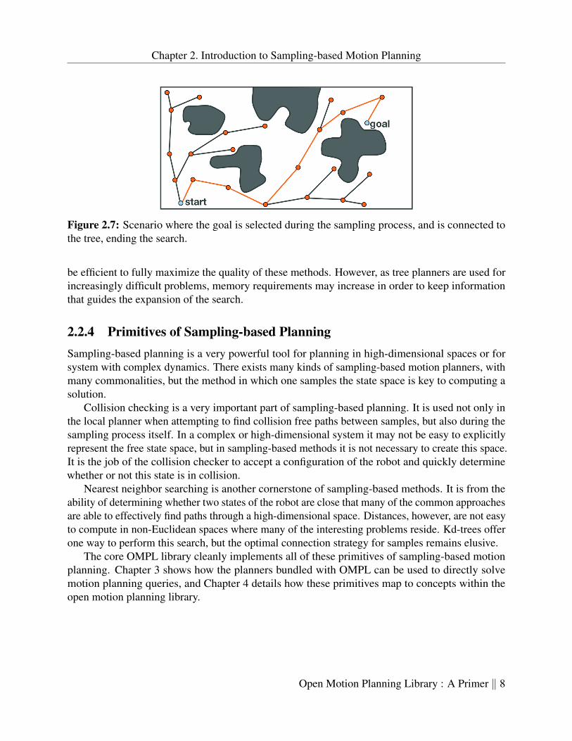
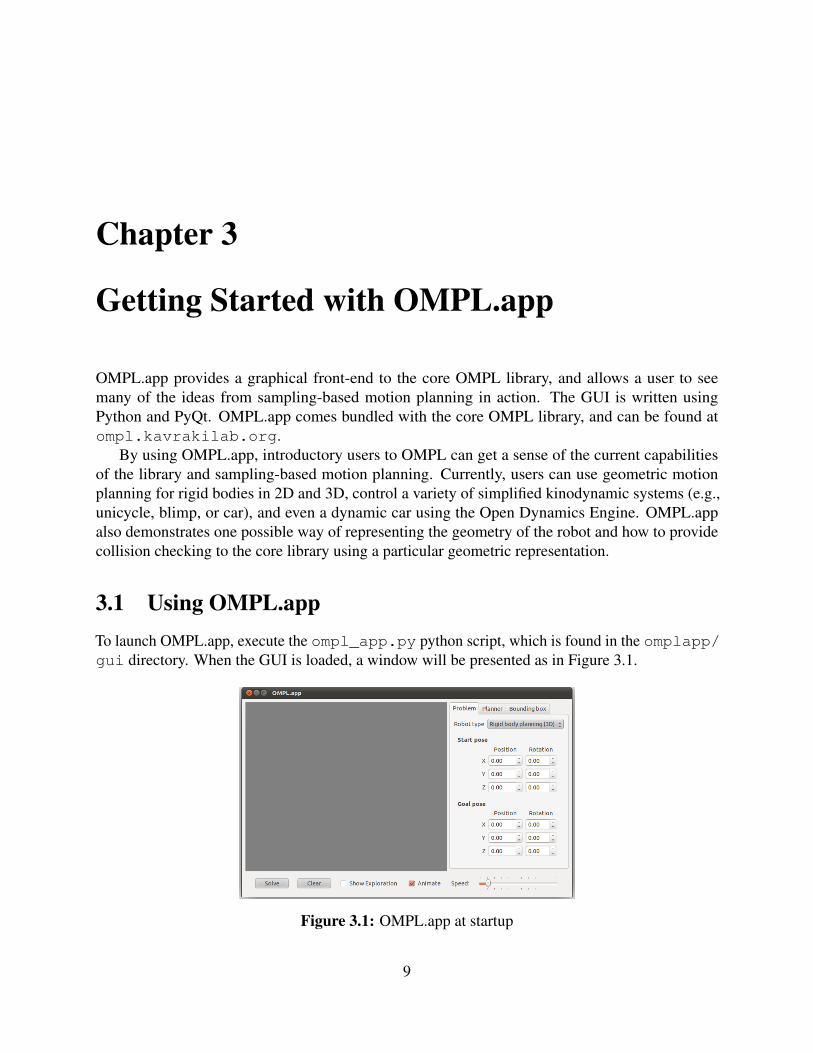
goal to the existing tree, then the search is complete; a path through the free state space has beenfound from the start to the goal. Figure 2.6 shows a case where the goal cannot be connected to thetree, and Figure 2.7 shows the case where the goal is connected, terminating the search.

Figure 2.6: Scenario where the goal is selected during the sampling process, but cannot beconnected to the tree. The closest node in the tree is obscured by an obstacle.

It is important to highlight the difference between the roadmap-based planners and the tree-basedplanners. The tree-based techniques are most suitable for single-query planning. These trees donot normally cover the free space in the same manner that a roadmap would. However, whenplanning with differential constraints, it is not easy to encode control information into an undirectededge. Controls are usually directed commands, and require a specific pre-condition in order fora particular control to be valid. Tree-based methods, on the other hand, excel at planning withcomplex dynamics because of the directed, acyclic nature of the underlying data structure. Controlinformation can be encoded for each edge of the tree, with the vertices of the tree satisfying theprerequisites for the valid controls.

Finally, it should be noted that many sampling-based approaches require a smaller memoryfootprint than other motion planners. The compactness of these planners stems from the samplingprocess itself, as well as the fact that no explicit representation of the state space is needed in orderto solve the problem. Storage and search of the underlying data structure (e.g., graph, tree) should



Figure 2.7: Scenario where the goal is selected during the sampling process, and is connected tothe tree, ending the search.

be efficient to fully maximize the quality of these methods. However, as tree planners are used forincreasingly difficult problems, memory requirements may increase in order to keep informationthat guides the expansion of the search.

2.2.4 Primitives of Sampling-based PlanningSampling-based planning is a very powerful tool for planning in high-dimensional spaces or forsystem with complex dynamics. There exists many kinds of sampling-based motion planners, withmany commonalities, but the method in which one samples the state space is key to computing asolution.

Collision checking is a very important part of sampling-based planning. It is used not only inthe local planner when attempting to find collision free paths between samples, but also during thesampling process itself. In a complex or high-dimensional system it may not be easy to explicitlyrepresent the free state space, but in sampling-based methods it is not necessary to create this space.It is the job of the collision checker to accept a configuration of the robot and quickly determinewhether or not this state is in collision.

Nearest neighbor searching is another cornerstone of sampling-based methods. It is from theability of determining whether two states of the robot are close that many of the common approachesare able to effectively find paths through a high-dimensional space. Distances, however, are not easyto compute in non-Euclidean spaces where many of the interesting problems reside. Kd-trees offerone way to perform this search, but the optimal connection strategy for samples remains elusive.

The core OMPL library cleanly implements all of these primitives of sampling-based motionplanning. Chapter 3 shows how the planners bundled with OMPL can be used to directly solvemotion planning queries, and Chapter 4 details how these primitives map to concepts within theopen motion planning library.


Chapter 3

Getting Started with OMPL.app

OMPL.app provides a graphical front-end to the core OMPL library, and allows a user to seemany of the ideas from sampling-based motion planning in action. The GUI is written usingPython and PyQt. OMPL.app comes bundled with the core OMPL library, and can be found atompl.kavrakilab.org.

By using OMPL.app, introductory users to OMPL can get a sense of the current capabilitiesof the library and sampling-based motion planning. Currently, users can use geometric motionplanning for rigid bodies in 2D and 3D, control a variety of simplified kinodynamic systems (e.g.,unicycle, blimp, or car), and even a dynamic car using the Open Dynamics Engine. OMPL.appalso demonstrates one possible way of representing the geometry of the robot and how to providecollision checking to the core library using a particular geometric representation.

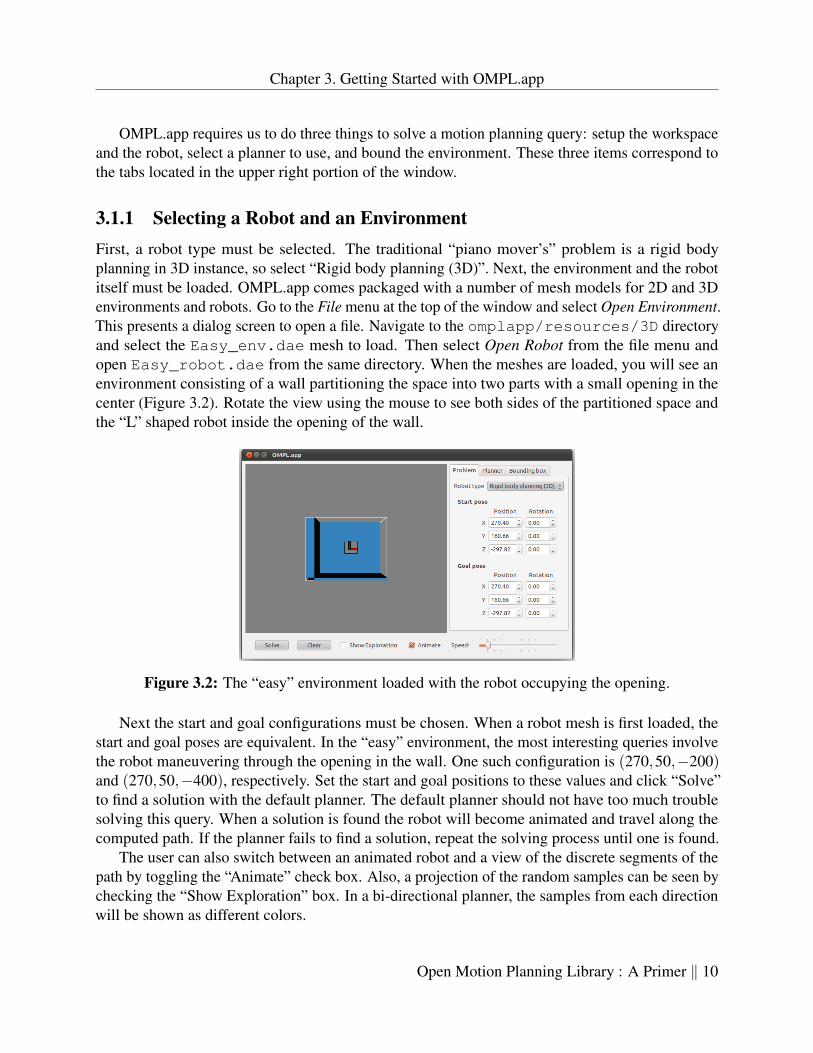
3.1 Using OMPL.appTo launch OMPL.app, execute the ompl_app.py python script, which is found in the omplapp/gui directory. When the GUI is loaded, a window will be presented as in Figure 3.1.

Figure 3.1: OMPL.app at startup

9

Chapter 3. Getting Started with OMPL.app

OMPL.app requires us to do three things to solve a motion planning query: setup the workspaceand the robot, select a planner to use, and bound the environment. These three items correspond tothe tabs located in the upper right portion of the window.

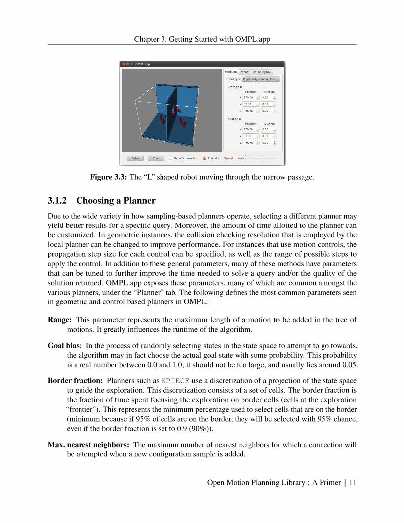
3.1.1 Selecting a Robot and an EnvironmentFirst, a robot type must be selected. The traditional “piano mover’s” problem is a rigid bodyplanning in 3D instance, so select “Rigid body planning (3D)”. Next, the environment and the robotitself must be loaded. OMPL.app comes packaged with a number of mesh models for 2D and 3Denvironments and robots. Go to the File menu at the top of the window and select Open Environment.This presents a dialog screen to open a file. Navigate to the omplapp/resources/3D directoryand select the Easy_env.dae mesh to load. Then select Open Robot from the file menu andopen Easy_robot.dae from the same directory. When the meshes are loaded, you will see anenvironment consisting of a wall partitioning the space into two parts with a small opening in thecenter (Figure 3.2). Rotate the view using the mouse to see both sides of the partitioned space andthe “L” shaped robot inside the opening of the wall.

Figure 3.2: The “easy” environment loaded with the robot occupying the opening.

Next the start and goal configurations must be chosen. When a robot mesh is first loaded, thestart and goal poses are equivalent. In the “easy” environment, the most interesting queries involvethe robot maneuvering through the opening in the wall. One such configuration is (270,50,−200)and (270,50,−400), respectively. Set the start and goal positions to these values and click “Solve”to find a solution with the default planner. The default planner should not have too much troublesolving this query. When a solution is found the robot will become animated and travel along thecomputed path. If the planner fails to find a solution, repeat the solving process until one is found.

The user can also switch between an animated robot and a view of the discrete segments of thepath by toggling the “Animate” check box. Also, a projection of the random samples can be seen bychecking the “Show Exploration” box. In a bi-directional planner, the samples from each directionwill be shown as different colors.



Figure 3.3: The “L” shaped robot moving through the narrow passage.

3.1.2 Choosing a PlannerDue to the wide variety in how sampling-based planners operate, selecting a different planner mayyield better results for a specific query. Moreover, the amount of time allotted to the planner canbe customized. In geometric instances, the collision checking resolution that is employed by thelocal planner can be changed to improve performance. For instances that use motion controls, thepropagation step size for each control can be specified, as well as the range of possible steps toapply the control. In addition to these general parameters, many of these methods have parametersthat can be tuned to further improve the time needed to solve a query and/or the quality of thesolution returned. OMPL.app exposes these parameters, many of which are common amongst thevarious planners, under the “Planner” tab. The following defines the most common parameters seenin geometric and control based planners in OMPL:

Range: This parameter represents the maximum length of a motion to be added in the tree ofmotions. It greatly influences the runtime of the algorithm.

Goal bias: In the process of randomly selecting states in the state space to attempt to go towards,the algorithm may in fact choose the actual goal state with some probability. This probabilityis a real number between 0.0 and 1.0; it should not be too large, and usually lies around 0.05.

Border fraction: Planners such as KPIECE use a discretization of a projection of the state spaceto guide the exploration. This discretization consists of a set of cells. The border fraction isthe fraction of time spent focusing the exploration on border cells (cells at the exploration“frontier”). This represents the minimum percentage used to select cells that are on the border(minimum because if 95% of cells are on the border, they will be selected with 95% chance,even if the border fraction is set to 0.9 (90%)).

Max. nearest neighbors: The maximum number of nearest neighbors for which a connection willbe attempted when a new configuration sample is added.



Every effort is made to set the defaults for these settings to values that are conducive in generalplanning environments. However, depending on the difficulty of the query, these settings may needto change to yield better performance. Consult the literature for the different planners to understandhow changing a specific parameter will change the behavior of a method in a particular instance.

3.1.3 Bounding the EnvironmentBy default, the robot is constrained to move inside a tight bounding box around the environment,the start pose, and the goal pose. The bounding box is visualized in OMPL.app as the white framearound the environment and robot. These bounds apply to a reference point for the robot; the originof the coordinate frame that defines its pose. This means that parts of the robot can stick outside thebounding box. It also means that if the reference point for your robot is far away from the robotitself, you can get rather unintuitive results. The reference point is whatever the origin is in themesh; OMPL.app is not using the geometric center of the mesh as the reference point.

3.1.4 Saving and Replaying Solution PathsOMPL.app also has the ability to save the current solution path and reload that path for viewingin the future. Once a problem has been solved, the solution found can be saved to a text file byselecting “Save Path” from the File menu. A save dialog will be presented to select a directory andfilename to save the path to. Similarly, the path can be reloaded and replayed by selecting “Loadpath” from the File menu. The environment or robot mesh data is not saved in this path file. Thesame environment and robot must be reselected by the user to replay the same path.

3.2 OMPL.app vs. OMPLOMPL.app builds upon the motion planning functionality in OMPL by specifying a geometricrepresentation for the robot and its environment, and provides a collision checking mechanism forthe representation to the existing planners in the library. OMPL.app makes use of open-sourcecollision checking libraries [9, 10]. The core Open Motion Planning Library does not explicitlyrepresent the robot or the environment, and it is up to the user to make this decision for theirparticular application.

OMPL has also been integrated with ROS. In ROS the robot and environment can be representedwith geometric meshes, but a model of the environment can also be obtained as a point cloud fromsensor data. ROS also provides a file format for specifying articulated mechanisms that, whenparsed, cause the appropriate state space for planning to be created.


Chapter 4

Planning with OMPL

The Open Motion Planning Library provides an abstract representation for all of the core con-cepts in motion planning, including the state space, control space, state validity, sampling, goalrepresentations, and planners. This chapter discusses OMPL and how its components relate to theideas from the motion planning literature. The first section discusses the design considerations ofthe library. The second section maps the components of OMPL to their logical equivalents in themotion planning literature. The third elaborates on the use of OMPL for solving motion planningqueries using sampling-based techniques composed from the objects described in Chapter 2. Thefourth section details the compilation of code written using OMPL, and the final discusses OMPL’sbenchmarking capabilities.

There exists a wide variety of documentation, tutorials, and other examples regarding the useof OMPL at ompl.kavrakilab.org. Specifically, the website has extensive resources forinstallation, hands-on tutorials, as well as the API documentation. Additionally, a group existsat sourceforge.net called “ompl-users”, which contains a forum for posting comments,questions, and bug reports.

4.1 Design ConsiderationsOMPL is flexible and applicable to a wide variety of robotic systems. As a consequence to thisflexibility, the library does not explicitly represent the geometry of the workspace or the robotoperating in it. This is deliberate since there exists a vast amount of file formats, data structures andother means of representation for robotic systems. As a result, the user must select a computationalrepresentation for the robot and provide an explicit state validity/collision detection method. Theredoes not exist a default collision checker in OMPL. This allows the library to operate with relativelyfew assumptions, allowing it to plan for a huge number of systems while remaining compact andportable.

A conscious effort is also made to limit the number of external dependencies necessary tocompile and execute the code in OMPL. The majority of the third party code utilized in the libraryused comes from Boost [11], which allows OMPL to function in most major operating systems.Currently, OMPL is supported on Linux and macOS. Windows installation of the core OMPL

13

Chapter 4. Planning with OMPL

library is also possible by compiling from source. Installation of OMPL.app on Windows can alsobe done, but this is recommended only for experienced Windows developers as the installation ofthe dependencies is challenging.

4.2 OMPL FoundationsChapter 2 showed that many sampling-based motion planners require a few similar componentsto solve a planning query: a sampler to compute valid configurations of the robot, a state validitychecker to quickly evaluate a specific robot configuration, and a local planner to connect twosamples along a collision free path. OMPL provides most of these components in similarly namedclasses. The following OMPL classes are analogous to ideas in traditional sampling-based motionplanners:

StateSampler The StateSampler class implemented in OMPL provides methods for uniformand Gaussian sampling in the most common state space configurations. Included in the libraryare methods for sampling in Euclidean spaces, the space of 2D and 3D rotations, and any combi-nation thereof with the CompoundStateSampler. The ValidStateSampler takes advantage of theStateValidityChecker to find valid state space configurations.

NearestNeighbors This is an abstract class that is utilized to provide a common interface to theplanners for the purpose of performing a nearest neighbor search among samples in the state space.The core library has several types of nearest neighbor search strategies at its disposal, includingGeometric Near-neighbor Access Trees (GNATs) [12] and linear searches. It is also possible to usean external data structure and supply the core library with this implementation.

StateValidityChecker The StateValidityChecker is tasked with evaluating a single state to deter-mine if the configuration collides with an environment obstacle and respects the constraints of therobot. A default checker is not provided by OMPL for reasons stated in Section 4.1. Since thiscomponent is an integral part of sampling-based motion planning it is necessary for the user toprovide the planner a callback to such a method to ensure that all configurations are feasible for therobot.

MotionValidator The MotionValidator class (analogous to the local planner) checks to see ifthe motion of the robot between two states is valid. At a high level, the MotionValidator must beable to evaluate whether the motion between two states is collision free and respects all the motionconstraints of the robot. OMPL contains the DiscreteMotionValidator, which uses the interpolatedmovements between two states (computed by the StateSpace) to determine if a particular motion isvalid. This is an approximate computation as only a finite number of states along the motion arechecked for validity (using the StateValidityChecker).



OptimizationObjective Certain motion planners can meet optimization objectives as well. Theseobjectives can implement different cost functions. The OptimizationObjective class provides anabstract interface to the relevant operations with costs that the planners need. There are multipledefault optimization objectives already implemented. For example, to minimize path length, aPathLengthOptimizationObjective (derived from OptimizationObjective) can be used.

ProblemDefinition A motion planning query is specified by the ProblemDefinition object. In-stances of this class define a start state and goal configuration for the robot, and the optimizationobjective to meet, if any. The goal can be a single configuration or a region surrounding a particularstate. Solutions to motion planning queries are also retrieved using this class.

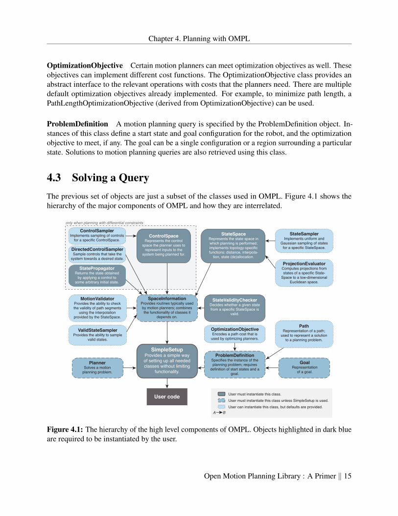
4.3 Solving a QueryThe previous set of objects are just a subset of the classes used in OMPL. Figure 4.1 shows thehierarchy of the major components of OMPL and how they are interrelated.

User code

StateSpaceRepresents the state space in which planning is performed; implements topology-specific functions: distance, interpola-

tion, state (de)allocation.

StateSamplerImplements uniform and

Gaussian sampling of states for a specific StateSpace.

ProjectionEvaluatorComputes projections from states of a specific State-

Space to a low-dimensional Euclidean space.

PathRepresentation of a path;

used to represent a solution to a planning problem.

GoalRepresentation

of a goal.

StateValidityCheckerDecides whether a given state from a specific StateSpace is

valid.

SpaceInformationProvides routines typically used by motion planners; combines the functionality of classes it

depends on.

MotionValidatorProvides the ability to check the validity of path segments

using the interpolation provided by the StateSpace.

ValidStateSamplerProvides the ability to sample

valid states.

PlannerSolves a motion

planning problem.

SimpleSetupProvides a simple way of setting up all needed classes without limiting

functionality.

ProblemDefinitionSpecifies the instance of the planning problem; requires

definition of start states and a goal.

A B

User must instantiate this class.User must instantiate this class unless SimpleSetup is used.User can instantiate this class, but defaults are provided.

only when planning with differential constraints

ControlSamplerImplements sampling of controls

for a specific ControlSpace.ControlSpace

Represents the controlspace the planner uses to

represent inputs to thesystem being planned for.

DirectedControlSamplerSample controls that take the

system towards a desired state.

StatePropagatorReturns the state obtained

by applying a control to some arbitrary initial state.

OptimizationObjective Encodes a path cost that is

used by optimizing planners.

Figure 4.1: The hierarchy of the high level components of OMPL. Objects highlighted in dark blueare required to be instantiated by the user.



The object oriented nature of OMPL allows the user to inherit from currently existing compo-nents or create brand new components to plan for a specific system. When solving a particularquery, the user is not required to instantiate all of the objects detailed in Figure 4.1. In fact, most ofthese objects have default implementations that are sufficient for general planning.

Geometric Planning For geometric motion planning, the user must define and instantiate thestate space object for the robot, and provide a start and goal configuration in that space to define themotion planning query. Any planner defined in the geometric namespace can then be employed tosolve the motion planning query. Some of these planners (as indicated by the planner specification)also follow optimization objectives.

Planning with Controls Like geometric planning, when planning with controls the user mustdefine and instantiate the state space for the robot, and provide a start and goal configuration. Inaddition, the user must define valid control inputs via a ControlSpace object, and provide a methodfor computing how the system state changes when applying valid controls using a StatePropagatorinstance. The user can use any planner in the control namespace to compute a solution.

SimpleSetup SimpleSetup provides a way to encapsulate the various objects necessary to solve ageometric or control query in OMPL. When using SimpleSetup, the user only supplies the statespace, start state, and goal state (and state propagator for planning with controls). Specifically,SimpleSetup instantiates the SpaceInformation, ProblemDefinition, and Goal objects. Additionally,SimpleSetup allows for the retrieval of all of these subcomponents for further customization. Thismeans that SimpleSetup does not inhibit any native functionality of OMPL, and ensures thatall objects are properly created before planning takes place. Moreover, SimpleSetup exposesfundamental function calls for ease of use. For example, the function “solve” from the Plannerclass is available in SimpleSetup, and it is not necessary for the user to extract the Planner from theSimpleSetup instance to do so.

4.4 Compiling Code with OMPLOnce a new planner, sampler, collision checker, or other motion planning component has been devel-oped, it is simple to integrate with OMPL for testing. There are two methods for compiling code withOMPL. If the base library is modified (e.g., a new planner is added to ompl/geometric/planners),simply re-run cmake to reconfigure the makefiles for that particular component of the code. If thenew code does not exist in a directory known to cmake, ompl/src/ompl/CMakeLists.txtwill need to be updated to search in the extra directory.

If OMPL has been installed, new code can be compiled independently from OMPL. The coreOMPL library can be linked into the final binaries using the traditional linking step. For example, ifcompiling with GCC, simply link the code with (-lompl), and direct the compiler to search theinstall directory for the library. A similar linking procedure can be employed with other compilers.



4.5 BenchmarkingThe ability to compare two or more planners has never been easier than with OMPL. OMPL providesa Benchmark class that attempts a specific query a given number of times, and allows the user to tryany number of planners. Additionally, the Benchmark instance can be configured to fail an attemptafter a specific amount of time or when the planner exhausts a given amount of memory. If multipleinstances of the same type of planner are to be benchmarked (e.g., with different sets of settings),changing the planner name is a good idea (Planner::setName() function), so that the results can bedistinguished.

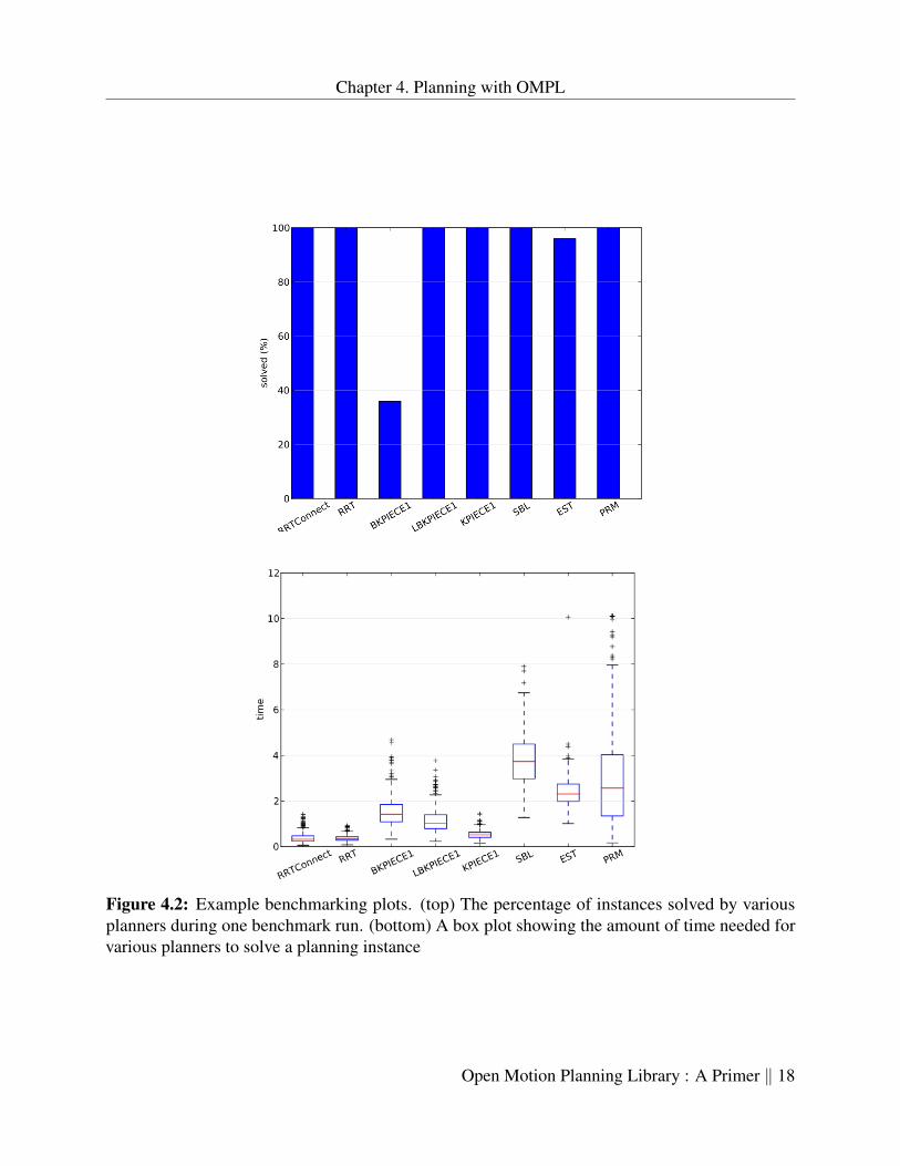
When the benchmarking has finished, the Benchmark instance will write a log file to the currentworking directory containing information regarding every planning attempt. OMPL is packagedwith a Python script to parse this log file and create an SQL database with the planning information.The Python script can also query this database and generate a series of plots using matplotlib, likethose in Figure 4.2.



Figure 4.2: Example benchmarking plots. (top) The percentage of instances solved by variousplanners during one benchmark run. (bottom) A box plot showing the amount of time needed forvarious planners to solve a planning instance


Chapter 5

Advanced Topics in OMPL

This chapter explains some of the more advanced features of OMPL. This section is not meant toexplain all of the expert level concepts, but to give the user an idea about some commonly usedoptional features of the library and how they can be included in the code. API documentationis updated regularly at ompl.kavrakilab.org, and includes the following concepts, amongothers.

5.1 State Space ConstructionOMPL provides implementations for several common states spaces, including Rn for Euclideanspaces and SO(2) and SO(3) for the space of rotations in 2D and 3D respectively. Many systemsoperate in spaces that are combinations of Rn and orientations. For example, the classic “pianomover’s” problem operates in SE(3), which is a combination of R3 and SO(3). OMPL contains animplementation of the SE(2) and SE(3) state spaces for such instances.

In complex systems, like highly articulated robot arms, it is infeasible to enumerate all possiblestate spaces. However, the state spaces in many of these systems can be decomposed into smallerspaces (like the SE(3) example). To accommodate this, OMPL allows for the construction of suchspaces through the CompoundStateSpace class, which allows state spaces to be formed from acombination of their subcomponents. The existing state spaces all provide operator overloads forthe ‘+’ and ‘−’, allowing readable and intuitive code to be written when constructing such spaces.

5.2 Planner CustomizationIn the motion planning literature, there exist many variants of the classical planning algorithmsthat change only one component of the planning algorithm in order to achieve benefits in certaininstances. Many of the planners that come bundled with OMPL are highly customizable, and insome cases it isn’t necessary to derive a new planner from the existing code base to recreate one ofthese variations or test a new idea or algorithm.

19

Chapter 5. Advanced Topics in OMPL

An easy example is the nearest neighbor search performed in nearly all of the planners to find theclosest existing state to a newly generated random sample. There are many algorithms to performthis search—both exact and approximate—and evaluating the best approach for one particularsystem can become time consuming. The PRM and RRT planners (among others) both provide ahook to replace the default nearest neighbor search with a user supplied object that derives from theabstract NearestNeighbor class. This allows users to develop compact and portable componentsfor differing nearest neighbor schemes and test them without creating unnecessary planner objectsthat are simply one-off from one another. Similar possibilities exist not only with nearest neighborsearching, but also in other planning components, like state sampling and connection strategies.

5.3 Python BindingsUsers of OMPL are not bound to C++. Most of the API is exposed through a set of Python bindingsfrom which users can create Python scripts to solve motion planning queries. These bindings arecompiled separately from the OMPL core library, and require Py++ and Boost.Python for correctoperation. Ensure that these dependencies exist before installing OMPL to create the bindings. ThePython bindings are still considered an experimental feature and all API documentation is for theC++ API (although we have tried to keep the python API as similar as possible). The easiest way toget started with the python bindings is by looking at a few of the demo programs.

The bindings are separated by ompl namespaces into python modules contained within oneparent ompl module. For example, to use a geometric motion planner from OMPL, the base andgeometric modules must be imported:from ompl import basefrom ompl import geometric

There are some subtle and some not-so-subtle differences between the C++ and Python APIsdue to the differences between the two programming languages. A user checking the OMPL C++API must note the following discrepancies when writing a program in Python:

• An STL vector of int’s is of type vectorInt in Python (analogously for other types).

• The C++ class State has been renamed AbstractState, while the C++ class ScopedState<> iscalled State in Python.

• The C++ class ScopedState<RealVectorStateSpace> is called RealVectorState. The Scoped-State’s for the other pre-defined state spaces have been renamed analogously.

• The C++ class RealVectorStateSpace::StateType has been renamed to RealVectorStateInternal(analogously for the other state space types), to emphasize that a user should really be usingRealVectorState.

• Use the “()” operator on a ScopedState in Python to retrieve a reference to a C++ State.

• The print method (for classes that have one) is mapped to the special python method __str__,so a C++ call like foo.print(std::cout) becomes print foo in python. Similarly,


Chapter 5. Advanced Topics in OMPL

a C++ call like foo.printSettings(std::cout) becomes print foo.settings()in python.

• The signature of the state validity checker is changed. In python the state validity checker hasthe following form:

def isStateValid(spaceInformation, state):return spaceInformation.satiesfiesBounds(state)


Bibliography

[1] Jean-Claude Latombe. Robot Motion Planning. Kluwer Academic Publishers, Norwell, MA,USA, 1991.

[2] Howie Choset, Kevin M. Lynch, Seth Hutchinson, George A Kantor, Wolfram Burgard,Lydia E. Kavraki, and Sebastian Thrun. Principles of Robot Motion: Theory, Algorithms, andImplementations. MIT Press, Cambridge, MA, June 2005.

[3] Steven M. LaValle. Planning Algorithms. Cambridge University Press, New York, NY, USA,2006.

[4] Lydia E. Kavraki, Petr Svestka, Jean-Claude Latombe, and Mark H. Overmars. Probabilisticroadmaps for path planning in high-dimensional configuration spaces. IEEE Transactions onRobotics and Automation, 12(4):566–580, 1996.

[5] Steven M. LaValle and James J. Kuffner. Randomized kinodynamic planning. InternationalJournal of Robotics Research, 17(5):378–400, 2001.

[6] David Hsu, Jean-Claude Latombe, and Rajeev Motwani. Path planning in expansive configura-tion spaces. International Journal of Computational Geometry and Applications, 9(4/5):495–512, 1999.

[7] Gildardo Sanchez and Jean-Claude Latombe. A single-query bi-directional probabilisticroadmap planner with lazy collision checking. In Robotics Research, volume 6 of SpringerTracts in Advanced Robotics, pages 403–417. 2003.

[8] Ioan Sucan and Lydia E. Kavraki. A sampling-based tree planner for systems with complexdynamics. IEEE Transactions on Robotics, 28(1):116–131, 2012.

[9] Eric Larsen, Stefan Gottschalk, Ming C. Lin, and Dinesh Manocha. Fast proximity querieswith swept sphere volumes. In IEEE International Conference on Robotics and Automation,pages 3719–3726, 2000.

[10] Jia Pan, Sachin Chitta, and Dinesh Manocha. FCL: A general purpose library for collision andproximity queries. In IEEE International Conference on Robotics and Automation, May 2012.

[11] http://www.boost.org/.

22

BIBLIOGRAPHY

[12] Sergey Brin. Near neighbor search in large metric spaces. In Proc. 21st Conf. on Very LargeDatabases, pages 574–584, 1995.


Open Motion Planning Library: A Primer - OMPLompl.kavrakilab.org/OMPL_Primer.pdf · Open Motion Planning Library: A Primer Kavraki Lab Rice University ompl.kavrakilab.org November

Documents