Ontario stream segmentation and characterization using Arc Hydro WSC Report No. 03-2006 September 2006 Watershed Science Centre. Trent University. Symons Campus 1600 West Bank Drive, Peterborough, Ontario K9J 7B8. www.trentu.ca/wsc

Welcome message from author
This document is posted to help you gain knowledge. Please leave a comment to let me know what you think about it! Share it to your friends and learn new things together.
Transcript
Ontario stream segmentation and characterization using Arc Hydro
WSC Report No. 03-2006
September 2006
Watershed Science Centre. Trent University. Symons Campus 1600 West Bank Drive, Peterborough, Ontario K9J 7B8.
www.trentu.ca/wsc
Ontario stream segmentation and characterization using Arc Hydro 2
Copyright The documents distributed by the Watershed Science Centre have been provided by the contributing authors as a means to ensure timely dissemination of scholarly and technical work on a non-commercial basis, which is Copyright protected. For such material, the submitting authors or other copyright holders retain rights for reproduction or redistribution. All persons reproducing or redistributing this information are expected to adhere to the terms and constraints invoked by the copyright holder. Permission is granted for the use of this information provided proper acknowledgement is given to the source using the following reference:
Schmidt, B.. 2006. Ontario stream segmentation and characterization using Arc Hydro. Watershed Science Centre, Trent University, Ontario, Canada. WSC Report 03-2006.
Disclaimer of Liability For documents, publications and databases available from the Watershed Science Centre, we do not warrant or assume any legal liability or responsibility for the accuracy, completeness, or usefulness of any information, apparatus, product, or process disclosed.
© Watershed Science Centre, 2006.
Ontario stream segmentation and characterization using Arc Hydro 3
Acronyms ............................................................................................................ 5
Definitions........................................................................................................ 5 1 Introduction.................................................................................................. 6
1.1 Existing Segmentation and Characterization Methods........................ 6 1.2 Applying the Arc Hydro Framework ..................................................... 7 1.3 System Requirements ......................................................................... 8 1.4 General Process Organization............................................................. 9 1.5 Typographic and Method Conventions.............................................. 10 1.6 Example Scenario ............................................................................. 10
2 Data Preprocessing................................................................................... 10 2.1 File Structure ..................................................................................... 10 2.2 Data Acquisition................................................................................. 11 2.3 Installing Arc Hydro ........................................................................... 12 2.4 Spatial Analyst Settings..................................................................... 12 2.5 Study Area Definition......................................................................... 12 2.6 Data Standardization ......................................................................... 13
2.6.1 EFDIR Raster ............................................................................ 13 2.6.2 EFDIR Streams Raster .............................................................. 14 2.6.3 Digital Elevation Model .............................................................. 14 2.6.4 Landcover Rasters..................................................................... 15 2.6.5 Geology Polygons...................................................................... 16 2.6.6 NRVIS Water Area Polygons..................................................... 18 2.6.7 NRVIS Water Virtual Flow Lines................................................ 18 2.6.8 NRVIS Drainage Lines / Points.................................................. 18 2.6.9 MNR Dam Points ....................................................................... 19 2.6.10 Other Barrier Lines / Points ....................................................... 19 2.6.11 XY Coordinate Rasters .............................................................. 19
3 Longitudinal Segmentation........................................................................ 20 3.1 Confluences....................................................................................... 20
3.1.1 Real Confluences ...................................................................... 21 3.1.2 Virtual Confluences.................................................................... 21 3.1.3 Combined Confluences ............................................................. 22
3.2 Lakes ................................................................................................. 25 3.2.1 Simplification.............................................................................. 25 3.2.2 Segmentation............................................................................. 27 3.2.3 Eliminating Discontinuities ......................................................... 28
3.3 Barriers .............................................................................................. 30 3.3.1 Alignment................................................................................... 31 3.3.2 Insertion ..................................................................................... 31
4 Network ..................................................................................................... 33 4.1 Generation......................................................................................... 33 4.2 Post-processing................................................................................. 34
4.2.1 Adding Attribute Fields............................................................... 34 4.2.2 Identifying Virtual Lake Segments ............................................. 36 4.2.3 Identifying Virtual Lake Confluences and Lake Outlets ............. 37 4.2.4 Transferring Confluence Information ......................................... 37 4.2.5 Generating Stream Order .......................................................... 38 4.2.6 Generating Barrier Attributes ..................................................... 39
5 Landscape Characterization...................................................................... 40 5.1.1 Spatial Scales ............................................................................ 42
Ontario stream segmentation and characterization using Arc Hydro 4
5.1.2 ArcMap Advanced Settings for Field Calculations..................... 42 5.1.3 Reach Centre-line Characteristics (RCCs) ................................ 42 5.1.4 Reach Contributing Areas (RCAs)............................................. 45 5.1.5 Total Drainage Areas (TDAs) .................................................... 46 5.1.6 Calculating the Percentage Fields ............................................. 49
Appendix 1: Map Examples............................................................................... 51 Appendix 2: Data Sources and Descriptions..................................................... 63 Appendix 3: Advanced ArcMap Utilities ............................................................ 72 Appendix 4: Classification Literature ................................................................. 74 References ........................................................................................................ 82
Ontario stream segmentation and characterization using Arc Hydro 5
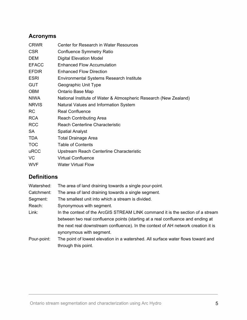
Acronyms CRWR Center for Research in Water Resources CSR Confluence Symmetry Ratio DEM Digital Elevation Model EFACC Enhanced Flow Accumulation EFDIR Enhanced Flow Direction ESRI Environmental Systems Research Institute GUT Geographic Unit Type OBM Ontario Base Map NIWA National Institute of Water & Atmospheric Research (New Zealand) NRVIS Natural Values and Information System RC Real Confluence RCA Reach Contributing Area RCC Reach Centerline Characteristic SA Spatial Analyst TDA Total Drainage Area TOC Table of Contents uRCC Upstream Reach Centerline Characteristic VC Virtual Confluence WVF Water Virtual Flow
Definitions Watershed: The area of land draining towards a single pour-point. Catchment: The area of land draining towards a single segment. Segment: The smallest unit into which a stream is divided. Reach: Synonymous with segment. Link: In the context of the ArcGIS STREAM LINK command it is the section of a stream between two real confluence points (starting at a real confluence and ending at the next real downstream confluence). In the context of AH network creation it is synonymous with segment. Pour-point: The point of lowest elevation in a watershed. All surface water flows toward and through this point.
Ontario stream segmentation and characterization using Arc Hydro 6
1 Introduction Resource managers have attempt to partition riverine landscapes into ecological meaningful units for decades (Lotspeich, 1980; Frissell et al; 1986, Seelbach et al., 1995; Snelder and Hughey, 2005). Recent advances in spatial datasets and geodatabase have allowed water resource managers to examine river systems as spatially aware networks while the increasing resolution of base data (e.g. DEMs) have allowed hydrologic GIS analyses to be performed at finer detail. The landscape character of the underlying stream bed, the reach contributing area and the entire upstream drainage area of a reach can now be collected with relative ease using existing tools such as Arc Hydro for ArcGIS. The characteristics collected at these varying scales will be useful for the development of a hierarchical linear mosaic of the landscape. Advanced datasets, such as the enhanced flow direction raster, have made it possible to seamlessly use mapped OBM hydrography in conjunction with synthetically derived stream networks. This integration enhances the utility of the final analysis output by allowing the direct linking of the results to real world features. Previous stream characterization work has focused on the underlying stream bed and/or utilized segmentation methods that are based on only stream confluences (see section 1.1). The methods outlined in this report combine both advanced longitudinal stream segmentation concepts with advanced characterization methods that are geared toward a landscape aware, hierarchical landscape-based classification system. The characterization methods have been designed to allow any raster attribute data to be used to meet future needs of additional landscape parameters, when they become required. The focus of this report is to describe the methods for segmenting and collecting the landscape characteristics for the segments. The classification of the stream segments into on physical and ecologically homogenous categories is not included and is best left to the expertise of ecologists.
1.1 Existing Segmentation and Characterization Methods River Environment Classification – REC (New Zealand Ministry for the Environment) This segmentation process employed by this classification method uses a confluence-only based approach. The created reaches are then utilizes to produce a hierarchical linear mosaic of landscape drainage areas. The hierachical nature of different scales of this classification attempt is to capture the interaction of processes that operate at varying scales form valley slopes to total upstream area (Snelder and Biggs, 2002). The output of the REC is supplied in the form of GIS data layer that contains the stream network of New Zealand at a scale of 1:50,000 and its associated reach characteristic attribute data (Snelder et al., 2004). GIS Tools for Stream and Lake Classification and Watershed Analysis (Nature Conservancy Freshwater Initiative)
Ontario stream segmentation and characterization using Arc Hydro 7
This method combines a suite of different tools, programmed using three different languages into one methodology. These tools do not have a common interface and are tied together by the methods outlined by FitzHugh (2005). The stream segments used for the characterization process are based on confluences-only. The author recommends that only experienced GIS user apply the methods due to the advanced knowledge required to effectively operate the three components in unison. This set of tools is being used by the Nature Conservancy in the United States for its freshwater ecoregional planning process. The output is available at a scale of 1: 100,000 for a large part of the United States (FitzHugh, 2005). Aquatic Landscapes Inventory Software – ALIS (Ontario Ministry of Natural Resources) This method is comprised of a software tool developed using Visual Basic for Applications (VBA) programming embedded within the ESRI ArcGIS 8.1 environment (Stanfield and Kuyvenhoven, 2002). The ALIS software was developed to assist in characterizing areas of Ontario using a set of landscape characteristics and their corresponding significant ecological thresholds. The tool segments streams longitudinally using a variety of factors and then delineates contributing areas from the individual pour-points on the stream network. Total upstream area characteristics are not included in the classification process. Ontario Rivers and Streams Segmentation – ORSECT (Ontario Ministry of Natural Resources) This method has been partially developed but is not completed (on hold) at this time. The goal, once finished, was to provide an automated GIS tool that would segment streams based on predefined and user defined spatial criteria. This method is intended to segment at the stream centre line level only and does not allow reach contributing areas or upstream drainage area to be characterized. Landscape-Based Ecological Classification System For River Valley Segments in Lower Michigan - MI-VSEC1.0 (Michigan Department of Natural Resources) This method segments rivers into fundamental units termed valley segments for the lower part of state of Michigan. These valley segments are generated using physical landscape based parameters and are characterized at the underlying reach centre-line and reach contributing area scale. Total drainage area characteristics were not collected. Classification of the segments was performed by local ecologists working to link characteristics with biological assemblages (Seelbach et al., 1997)
1.2 Applying the Arc Hydro Framework Arc Hydro (AH) is a GIS based storage, modelling and analysis framework for use with water resource planning. AH utilizes the Environmental Systems Research Institute (ESRI) geodatabase structure to store spatial features, relationships between features and information
Ontario stream segmentation and characterization using Arc Hydro 8
tables. AH includes a set of robust and efficient tools and provides several major advantages for the purposes of stream segmentation and characterization which include:
• Accumulation of the landscape characteristics of the total upstream drainage area for every segment of the stream network without any need for programming new custom GIS tools.
• Creation of drainage points data including inlets/outlets for each segment’s reach contributing area allowing for confluence effect magnitude assessment.
• Offers a well designed and structured data storage and management environment. • Operates within the ESRI ArcGIS environment which is the standard GIS platform of
the MNR and many other agencies in Ontario which effectively leverages existing expertise, spatial data and allowing easy data sharing and integration.
• The AH framework and tools are constantly being improved and developed further by the CRWR and ESRI eliminating the need to maintain custom in-house tools.
It is recommended that when using high resolution data such as 10m rasters and 1:10,000 vectors that the drainage area to be processed does not exceed 1000 km2. This will greatly reduce computer processing times and to avoid running into potential software limitations. The recommended maximum drainage areas can be increased as DEM and vector resolution decrease (e.g. 20m DEM and 1:20,000 vectors etc.). In cases where larger drainage areas are required AH provides methods and tools to split large areas into smaller, more manageable units which can then be merged into a large overarching geodatabase. This allows the user to study larger drainage areas in more manageable portions while still being able to create a final unified model. A key component of the methods described by this report is the Enhanced Flow Direction (EFDIR) raster. The OMNR Water Resources Information Program (WRIP) created the EFDIR raster which aligns the synthetic streams created using the D8 flow direction algorithm with mapped (known) streams. The segmentation methods outlined in this report go above and beyond the original design of the AH network creation tools. These tools were designed to create simple segments based on real stream confluences only. Introducing other segmentation rules adds a higher degree of complexity to the final stream network and also requires a higher degree of user expertise in the creation process, since the AH tools do not contain built-in functions to handle some of these new rules. However, once this network has been created the convenient and existing attribute collection and data management tools of AH can easily be leveraged without requiring further development.
1.3 System Requirements ArcGIS 9.x with an ArcInfo license and a Spatial Analyst extension license is required for use the exact methods described in this report. ArcGIS 8.x could be used but not all the tools are
Ontario stream segmentation and characterization using Arc Hydro 9
available in this version. It would be up to the user to acquire third party scripts and tools that perform equivalent tasks and to modify the methods to produce similar results. It is recommended to use a dual core or dual processor workstation since this will run the more time consuming analyses (e.g. attribute accumulation) without tying up the workstation completely.
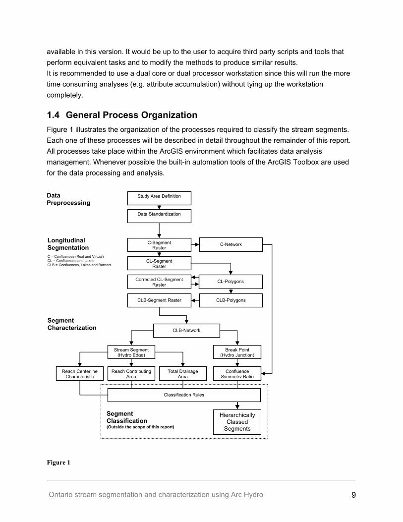
1.4 General Process Organization Figure 1 illustrates the organization of the processes required to classify the stream segments. Each one of these processes will be described in detail throughout the remainder of this report. All processes take place within the ArcGIS environment which facilitates data analysis management. Whenever possible the built-in automation tools of the ArcGIS Toolbox are used for the data processing and analysis.
Figure 1
C-Segment Raster
CL-Segment Raster
CL-PolygonsCorrected CL-Segment Raster
CLB-PolygonsCLB-Segment Raster
CLB-Network
Longitudinal Segmentation
Segment Characterization
Reach Centerline Characteristic Reach Contributing
Area Total Drainage Area
Hierarchically Classed
Segments
C = Confluences (Real and Virtual) CL = Confluences and Lakes CLB = Confluences, Lakes and Barriers
Confluence Symmetry Ratio
C-Network
Stream Segment (Hydro Edge) Break Point
(Hydro Junction)
Segment Classification (Outside the scope of this report)
Classification Rules
Data Preprocessing
Data Standardization
Study Area Definition
Ontario stream segmentation and characterization using Arc Hydro 10
1.5 Typographic and Method Conventions Italicized text - File names, Table names, Tool names, Folder locations, Menu Items Square Brackets - [ ] - denote a field name in an attribute table or stand-alone table or a input raster name in a Spatial Analyst Raster Calculator expression Braces - { } - denote the generic form of a file/field name. It is used when a processing step must be repeated several times with identical parameters except the input and/or output file/field name changes. Courier Font - Field/Raster Calculator Expressions, Program Code General Rules: 1. If a setting parameter or option of a tool is not mentioned it should be left at the default
setting. 2. Anytime new raster data is created and added to the TOC automatically remove the raster
data from the TOC and add it back again. This ensures that the names of the raster layers in the TOC match their filename. These TOC layer names are referenced by many of the Raster Calculator expressions and need to be identical to those expressions in order for them to function properly.
1.6 Example Scenario The segmentation and characterization of Credit River watershed in southern Ontario has been completed using the methods described in this report. This exemplary data serves to lend insight into the methods and to illustrate the output which can be expected. The Credit River watershed was chosen because the EFDIR raster data was available for immediate use. Since the time that this work was started the EFDIR data have now also been processed and are available in other areas of Ontario. Several preformatted ArcMap documents are provided to demonstrate the output of the described methods. These can be found in the Maps folder of the included example data CD-ROM.
2 Data Preprocessing
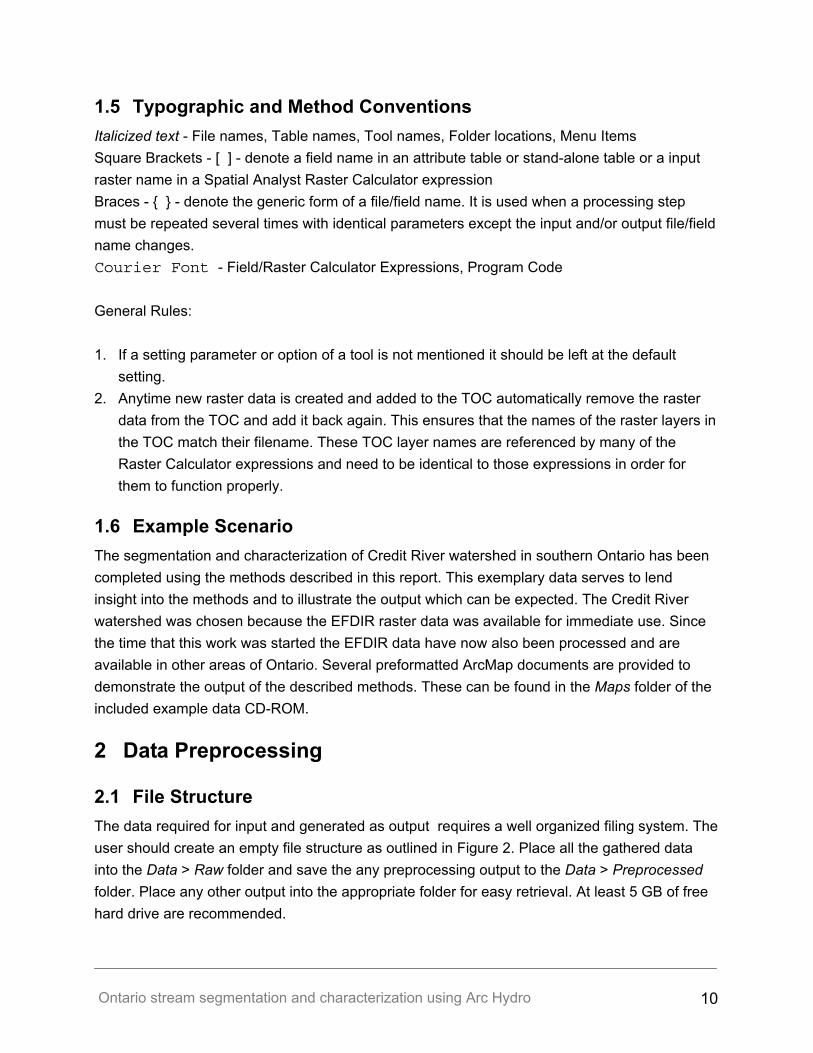
2.1 File Structure The data required for input and generated as output requires a well organized filing system. The user should create an empty file structure as outlined in Figure 2. Place all the gathered data into the Data > Raw folder and save the any preprocessing output to the Data > Preprocessed folder. Place any other output into the appropriate folder for easy retrieval. At least 5 GB of free hard drive are recommended.
Ontario stream segmentation and characterization using Arc Hydro 11
Figure 2
2.2 Data Acquisition Gather the raw data for the study area and place them into the Data > Raw folder. It is important that the spatial extent of every dataset covers the entire spatial extent of the study area. The data, with the exception of the Quaternary Geology and the Landcover28 data, are not available at the full extent of the province of Ontario, but are divided into smaller more manageable sections. Please refer to Appendix 2 for more details on available spatial extent of these sections and descriptive data concerning each dataset. Raster Data:
• Enhanced Flow Direction (EFDIR) raster • Enhanced Flow Direction Streams raster • Provincial Digital Elevation Model • Landcover 28 raster • Landcover 2000 raster
Vector Data: • NRVIS Water Area polygons • NRVIS Water Virtual Flow lines • NRVIS Drainage lines • Surficial Geology of Southern Ontario polygons • Quaternary Geology of Ontario polygons • MNR Dam points • Conservation Authority Dam points • Other Barrier structures points
Ontario stream segmentation and characterization using Arc Hydro 12
2.3 Installing Arc Hydro The user should obtain the latest version of Arc Hydro Tools available for download from http://www.crwr.utexas.edu/archydrotools/tools.html and run the setup.exe that is included with the package. The Arc Hydro toolbar can be turned on within ArcMap once the setup is complete. The version of Arc Hydro used is to test the segmentation and characterization methods is Arc Hydro beta8_08132004. Do not use earlier version since they may not work with the described methods.
2.4 Spatial Analyst Settings Uniformly formatted (size and alignment) output created with the Spatial Analyst (SA) Extension requires SA Options to be set correctly. Note that these settings are reset every time a new ArcMap document is created. It is important to check frequently that these settings remain changed. All raster data must be snapped to the extent of the EFDIR raster and share its cell size. Set the SA Options as follows • The SA output extent and cell size is initially set to match that of the raw EFDIR raster (e.g.
z17hw_efdb) until instructed otherwise. • Setting the working directory (folder) to the match the processing step being performed (see
the recommended file structure of Section 2.1). • No analysis mask is required. • The output data should automatically have its projection defined according to the coordinate
system of the current active data frame.
2.5 Study Area Definition The study area needs to be defined before any other work can be completed. This process requires the pour-point location and the raw EFDIR raster. The process’ output will be a polygon shapefile that defines the watershed boundary of the study area and its rectangular spatial extent. The watershed boundary and its rectangular extent will determine the size and extent of all subsequent preprocessed data.
1. Open a new ArcMap document and add the raw EFDIR raster and EFDIR Streams raster to the TOC
Note: The raw EFDIR raster will later be clipped to size of the study area. 2. Set the View > Data Frame Properties > Coordinate System to match the raw EFDIR
raster. 3. Save the ArcMap document as preprocessing.mxd in the Data > Preprocessed folder. Note: Save your ArcMap documents frequently.
Ontario stream segmentation and characterization using Arc Hydro 13
4. Open ArcCatalog and create a new empty point shapefile named StudyArea_PourPoint (File > New… > Shapefile) and set its coordinate system to match that of the raw EFDIR raster.
5. Add the empty StudyArea_PourPoint shapefile to the ArcMap TOC. 6. Start and edit session with the StudyArea_PourPoint layer as the Target. 7. Choose the Create New Feature as the Task and the Sketch tool in the editor toolbar. 8. Using the EFDIR Streams raster as a guide, place the arrow cursor on the outlet of the
study area (at the center of the outlet cell) and left-click to create the pour-point. 9. Stop editing and save the edits. 10. Delineate the study area watershed boundary using the Watershed tool (Spatial Analyst
Tools > Hydrology > Watershed) with the EFDIR raster and the StudyArea_PourPoint shapefile as inputs and name it Study_Wshed.
Note: This process can take a considerable amount of time to complete depending of the size of the study area and resolution of the EFDIR raster. 11. Convert the Study_Wshed raster to a vector polygon using the Raster to Features tool
(Spatial Analyst > Convert > Raster to Features function with the Generalize lines option unchecked. This process may create several small superfluous polygons along the boundary of the main watershed polygon.
12. Start and editing session with the Target being the StudyArea_Watershed polygons layer to remove the small superfluous polygons.
13. Select the main watershed (the largest polygon) on the map, then switch the selection and delete the selection. Only one polygon (the main watershed) should be left remaining.
14. Stop editing and save the edits.
2.6 Data Standardization All raster data, including rasterized vector data, must share the same spatial extent, projection and cell size. Ideally, all vector data should share a similar spatial scale, precision and accuracy. However, it is not always possible to obtain vector data from disparate sources and still meet these criteria. It is recommended that when using a combination of non-uniform data sets that the differences are well documented so that appropriate considerations can be made when using the results for decision making purposes. The required raw data will most likely exist at excessively large spatial extents when compared to the size of the study area. These extents must be reduced to match either the study area watershed boundary or its rectangular extent. The first dataset to be preprocessed must be the EFDIR raster since all subsequent datasets must aligned with it.
2.6.1 EFDIR Raster 1. Set the Spatial Analyst Options Extent to the StudyArea_Watershed polygon extent.
Ontario stream segmentation and characterization using Arc Hydro 14
2. Open the attribute table of the StudyArea_Watershed polygon and calculate the [ID] field to equal one (i.e. [ID] = 1).
3. Extract the study area EFDIR raster using the Extract by Mask tool (Spatial Analyst Tools > Extraction) using the raw EFDIR raster as input, the StudyArea_Watershed polygon as the clipping mask and name this new file efdir_clip.
4. Set the Spatial Analyst Options Extent to match the efdir_clip raster extent. Note: This extent setting must remain the same for the remainder of the procedures described in this report.
2.6.2 EFDIR Streams Raster 1. Extract the EFDIR Streams raster using the Extract by Mask tool (Spatial Analyst Tools >
Extraction) using the EFDIR Streams raster as input, the StudyArea_Watershed polygon as the clipping mask and name this new file streams_clip.
2.6.3 Digital Elevation Model 1. Create the clipping polygon from the rectangular spatial extent of the
StudyArea_Watershed polygon using the Feature Envelope to Polygon tool (Data Management > Features). Leave the Multipart option unchecked, use the StudyArea_Watershed polygon as input and name the output Clipping_Rectangle.
2. Add the required Digital Elevation Model (DEM) tiles to the ArcMap TOC using demtiles_{UTMzone} polygons as (Data > Raw folder) in the background as a guide.
3. . 4. Mosaic the DEM tiles together using the Mosaic to New Raster tool (Data Management
Tools > Raster) using the following parameters: • Input Rasters: List all input DEM tiles • Output Location: Drive:\{StudyAreaName}\Data\Preprocessed • Raster dataset name: dem_mosaic • Coordinate system: matching the EDFIR raster • Pixel Type: 8 bit unsigned • Cell size: matching the EFDIR raster • Mosaic Method: Mean • Mosaic Colormap Mode: FIRST
5. Extract the study area extent from the dem_mosaic raster using the Extract by Mask tool (Spatial Analyst Tools > Extraction) using the dem_mosaic raster as input, the Clipping_Rectangle polygon as the clipping mask and naming this new file dem_clip.
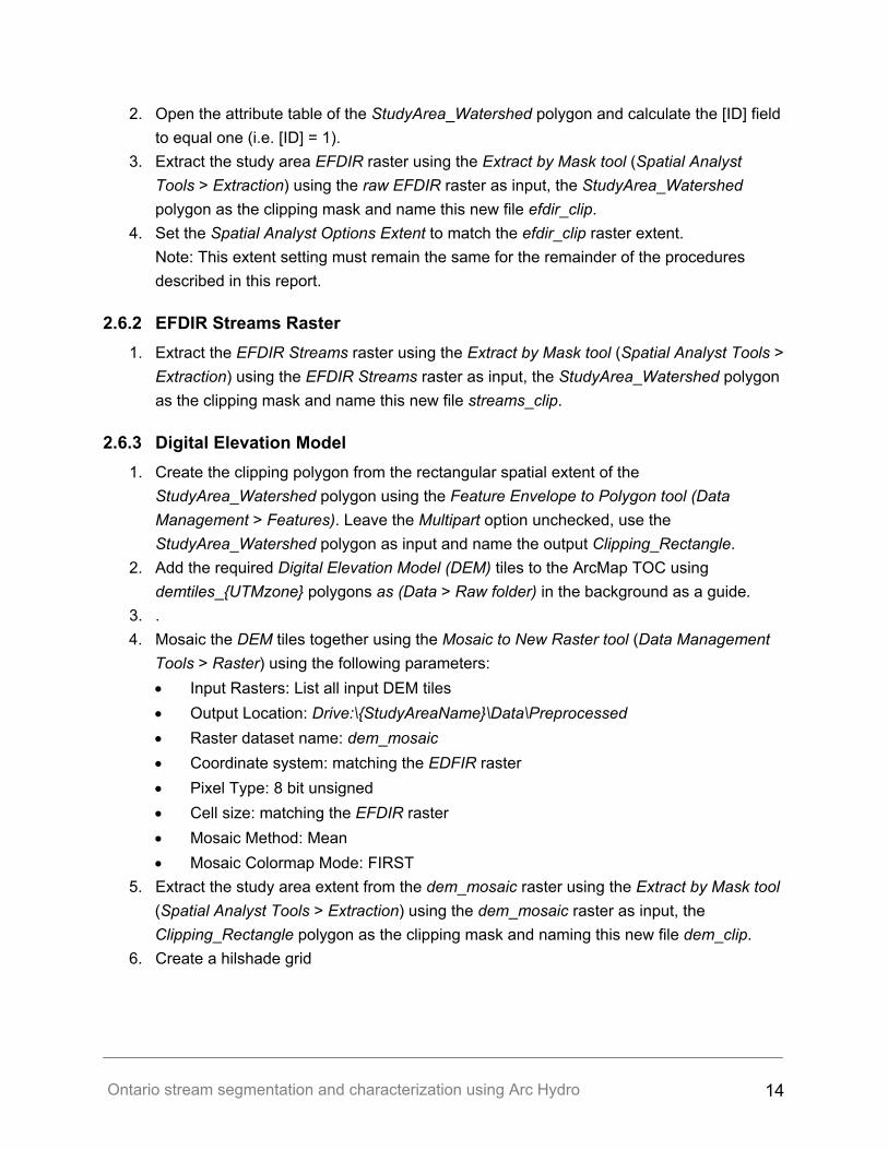
6. Create a hilshade grid
Ontario stream segmentation and characterization using Arc Hydro 15
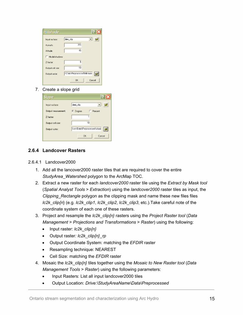
7. Create a slope grid
2.6.4 Landcover Rasters
2.6.4.1 Landcover2000
1. Add all the lancover2000 raster tiles that are required to cover the entire StudyArea_Watershed polygon to the ArcMap TOC.
2. Extract a new raster for each landcover2000 raster tile using the Extract by Mask tool (Spatial Analyst Tools > Extraction) using the landcover2000 raster tiles as input, the Clipping_Rectangle polygon as the clipping mask and name these new files files lc2k_clip{n} (e.g. lc2k_clip1, lc2k_clip2, lc2k_clip3, etc.).Take careful note of the coordinate system of each one of these rasters.
3. Project and resample the lc2k_clip{n} rasters using the Project Raster tool (Data Management > Projections and Transformations > Raster) using the following: • Input raster: lc2k_clip{n} • Output raster: lc2k_clip{n}_rp • Output Coordinate System: matching the EFDIR raster • Resampling technique: NEAREST • Cell Size: matching the EFDIR raster
4. Mosaic the lc2k_clip{n} tiles together using the Mosaic to New Raster tool (Data Management Tools > Raster) using the following parameters: • Input Rasters: List all input landcover2000 tiles • Output Location: Drive:\StudyAreaName\Data\Preprocessed
Ontario stream segmentation and characterization using Arc Hydro 16
• Raster dataset name: lc2k_mosaic • Coordinate system: matching the EFDIR raster • Pixel Type: 8 bit unsigned • Cell size: matching the EFDIR raster • Mosaic Method: FIRST • Mosaic Colormap Mode: First
2.6.4.2 Landcover28
1. Add the landcover28 raster to the ArcMap TOC. 2. Extract the landcover28 raster using the Extract by Mask tool (Spatial Analyst Tools >
Extraction) using the landcover28 raster as input, the Clipping_Rectangle polygon as the clipping mask and name this new file lc28_clip25m.
3. Project and resample the lc28_clip25m raster using the Project Raster tool (Data Management > Projections and Transformations > Raster) using the following: • Input raster: lc28_clip25m • Output raster: lc28_clip_rp • Output Coordinate System: matching the EFDIR raster • Resampling technique: NEAREST • Cell Size: matching the EFDIR raster
4. Clean the edges of the lc28_clip_rp raster using the Extract by Mask tool (Spatial Analyst Tools > Extraction) using the lc28_clip_rp raster as input, the Clipping_Rectangle polygon as the Clipping mask and name this new file lc28_prepro.
2.6.5 Geology Polygons
2.6.5.1 Surficial Geology of Southern Ontario
1. Convert the sgu_poly coverage to a shapefile using the Featureclass to Shapefile tool (Conversion Tools > to Shapefile) using the sgu_poly coverage as input and the Data > Preprocessed folder as the output destination (leave the default output name as sgu_poly polygon.shp).
2. Extract the sgu_poly polygons for the study area extent using the Clip tool (Data Management Tools > Extract) using the sgu_poly polygons as input, the Clipping_Rectangle polygon as the Clip features and name this new file sgu_clip. A Cluster tolerance does not need to be set.
3. Project the sgu_clip polygons using the Project tool (Data Management > Projections and Transformations > Feature) using the sgu_clip polygons as input, setting the Output Coordinate System to match the EFDIR raster and naming the output sgu_clip_projected.
4. Add the following new fields to the sgu_clip_projected table:
Ontario stream segmentation and characterization using Arc Hydro 17
• [PM_Code] (data type = text, length = 3) • [SM_Code] (data type = text, length = 3) • [PMSM_Code] (data type = integer)
5. One by one select the records for each of the unique PRIM_MAT types in the sgu_clip table and then calculate a unique number code (1, 2, 3 … n) in the [PM_Code] field for each PRIM_MAT type.
6. One by one select the records for each of the unique SINGLE_PRI types in the sgu_clip table and then calculate a unique number code (1, 2, 3 … n) in the [SM_Code] field for each SINGLE_PRI type.
7. Concatenate the SM_Code and PM_Code fields using the following VBA syntax: dim concatenated_string as string dim integer_Code as integer concatenated_string = [PM_Code] & [SM_Code] integer_Code = VAL(concatenated_string)
[PMSM_Code] = integer_Code 8. Convert the sgu_clip_projected polygons to a raster using the Features to Raster
function (Spatial Analyst Menu > Convert) using the [PMSM_Code] field as the Field, the Cell size matching the EFDIR raster and naming the output sgu_pmsm.
9. Turn on the sgu_clip_projected polygons and set the symbology to Hollow. Inspect the sgu_pmsm raster for map sheet boundary errors (please see Appendix 2). Make note of these errors and include them in any reports generated using this data.
2.6.5.2 Quaternary Geology of Ontario
1. Add the geology_ll polygons for the entire province to the ArcMap TOC. 2. Extract the geology_ll polygons for the study area extent using the Clip tool (Data
Management Tools > Extract) using the geology_ll polygons as the input, the Clipping_Rectangle polygon as the clipping mask, and name this new file geo1M_clip.
3. Project the geo1M_clip polygons using the Project tool (Data Management > Projections and Transformations > Feature) using the geo1M_clip polygons as input, setting the Output Coordinate System to match the EFDIR raster and naming the output geo1M.
4. Add the field [UName_Code] (data type = text, length = 3) to the geo1M table: 5. One by one select the records for each of the unique [UNIT_NAME] types in the geo1M
table and then calculate a unique number code (1, 2, 3 … n) in the [UName_Code] field for each [UNIT_NAME] type.
6. Convert the geo1M polygons to a raster using the Features to Raster function (Spatial Analyst Menu > Convert) using the [UName_Code] field as the Field, the Cell size matching the EFDIR raster and naming the output geo1M.
Ontario stream segmentation and characterization using Arc Hydro 18
2.6.6 NRVIS Water Area Polygons 1. Identify which MNR District areas are required to completely cover the
StudyArea_Watershed polygon using the MNR_Districts polygons (Data > Raw folder) in the background as a guide.
2. Place the MNR district Water Area polygons sections to the Raw > Data folder and rename them {MNR_district_name}_wpoly. Add these sections to the ArcMap TOC.
3. If more than one district was required then combine the {MNR_district_name}_wpoly polygon sections using the Merge tool (Data Management > General) using {MNR_district_name}_wpoly polygon sections as input and naming the output wpoly_merged.
4. Project the wpoly_merged polygons using the Project tool (Data Management > Projections and Transformations > Feature) using the wpoly_merged polygons as input setting the Output coordinate system to match the EFDIR raster and naming the output wpoly_merged_projected.
5. Extract the polygons of the study area watershed boundary using the Clip tool (Analysis Tools > Extract) using the wpoly_merged_projected polygons as input and the StudyArea_Watershed as the Clipping polygon and naming the output wpoly_preprocessed.
2.6.7 NRVIS Water Virtual Flow Lines 1. Add the UTM zone section of the Water Virtual Flow lines to the ArcMap TOC. 2. Extract the Water Virtual Flow lines of the StudyArea_Watershed polygon using the Clip
tool (Analysis Tools > Extract) using the Water Virtual Flow lines as input and the StudyArea_Watershed as the clipping polygon and naming the output vFlow_preprocessed.
Note: This data will never cross UTM zone boundaries by design.
2.6.8 NRVIS Drainage Lines / Points 1. Identify which MNR Regions are required to completely cover the study area watershed
boundary using the MNR_regions polygons (Data > Raw folder) in the background as a guide.
2. Add the identified MNR region sections of the Drainage Lines and Points to the ArcMap TOC.
3. Combine the individual region sections using the Merge tool (Data Management > General) using the individual region sections (list) as input and naming the output rawDLines_merged and rawDPoints_merged.
Note: If no merging is necessary then rename the lines and points to DLines_merged and DPoints_merged respectively.
Ontario stream segmentation and characterization using Arc Hydro 19
4. Project the DPoints_merged points and the DLines_merged using the Project tool (Data Management > Projections and Transformations > Feature) using the DPoints_merged points and the rawDLines_merged as input, setting the Output Coordinate System to match the EFDIR raster and naming the output DPoints_projected and DLines_projected.
5. Extract the DPoints_projected points and DLines_projected lines of the study area watershed boundary using the Clip tool (Analysis Tools > Extract) using the DPoints_projected and DLines_projected as input and the StudyArea_Watershed as the clipping polygon and naming the output DLines_clip and DPoints_clip.
6. Convert the DLines_clip to points using the Feature to Point tool (Data Management > Features) using the DLines_clip as input with the Inside option unchecked and naming the output DPointsfromLines.
7. Combine DPoints and the DPointsfromLines using the Merge tool (Data Management > General) using the DPoints and the DPointsfromLines as input and naming the ouptput DPoints_merged and naming the output DPoints_preprocessed.
2.6.9 MNR Dam Points 1. Identify which UTM zones are required to completely cover the StudyArea_Watershed
polygon. 2. Add the identified UTM zone sections of the Dam lines to the ArcMap TOC. Combine the
individual region sections using the Merge tool (Data Management > General) using the individual region sections (list) as input and naming the output mnrdamlines_merged.
3. Extract the dam lines of the study area watershed boundary using the Clip tool (Analysis Tools > Extract) using the mnrdamlines_merged as input and the StudyArea_Watershed as the clipping polygon and naming the output mnrdams_preprocessed.
2.6.10 Other Barrier Lines / Points For additional barrier lines and points (conservation authority dams, industrial dams, agricultural dams) use the same methods outlined in Section 2.6.8 and Section 2.6.9 above.
2.6.11 XY Coordinate Rasters These rasters will be used to calculate slope values using straight-line euclidean distance measurements.
1. Create a latitude and a longitude raster using the SA Raster Calculator using the following expressions:
xGRID = int($$xmap) yGRID = int($$ymap)
Ontario stream segmentation and characterization using Arc Hydro 20
3 Longitudinal Segmentation In order to divide a stream into segments, three key variables were chosen to represent the longitudinal changes that can abruptly influence the physical characteristics of stream environments. These variables are stream confluences, lakes on the stream network and physical barriers on the network. Segmentation using these three variables is handled by separate processes which result in a final source raster that is used as the basis for creating an AH geodatabase. The additional three landscape characteristics of surficial geology, landcover and slope were originally to be included in the longitudinal segmentation process, where intersections of the individual reach segments and threshold break-points for these three variables would result in further the splitting of the stream. However, after close examination of the high resolution data it was realized these processes would result in a large number of very small and meaningless stream segments and landscape area fragments. It was decided that segmenting the stream using confluences (real and virtual), lakes, and barriers (CLB segments) would provide a sufficient small enough tessellation of the landscape. It was also decided that characterizing the underlying geology, landcover and slope characteristics of the resulting CLB segments would be a more meaningful way of describing these attributes.
3.1 Confluences Confluences are included in the segmentation process since they represent points along the stream where water quantity and quality can suddenly change depending on the upstream area and landscape characteristics of the meeting segments. Real confluence (RC) points and virtual confluence (VC) points are identified. RC points are the locations were mapped (OBM) streams meet. VC points identify locations along the stream where a, DEM derived, high flow accumulation cell meets the mapped stream and no RC point exist at that location (i.e. a mapped stream does not exists to identify the high flow accumulation values). VC points could be indicative of areas where water is being drained to near surface or deep groundwater before being able to form a stream on the surface or a possible omission of a stream vector during the OBM mapping process. In either case VC points are locations of interest that should be investigated. VC points allow RC defined stream segments to be further subdivided into smaller segments using a physical, landscape aware method. A threshold flow accumulation must be determined above which VC points are created. The VC point creation threshold (VCt) is set equal to the median drainage area of the catchments created using the RC point segments. Confluence Symmetry Ratios (CSRs) is the ratio between the main channel (receiving stream) FA at the confluence and the contributing tributary channel (contributing stream) FA where tributary channel is the stream having the smaller FA at the confluence. The CSR is an indicator of the magnitude of influence that a tributary can potentially assert on the larger main channel stream. Individual contributing areas of small tributaries may have little or no impact on the larger main channel into which they flow. Cumulative (additive downstream)
Ontario stream segmentation and characterization using Arc Hydro 21
effects of consecutive, small hydrologically homogenous confluences on the receiving larger stream may also be considered once the final hydro network and characteristics have been established. Two seperate AH geodatabases will be created during this process one for real confluences and one for virtual confluences. The first geodatabase will provide RC point catchments area statistics (e.g. median area) output which will be used as inpu to the VC point creation process.
3.1.1 Real Confluences
1. Open a new ArcMap document and add the efdir_clip raster and the streams_clip raster and the to the ArcMap TOC and set the Spatial Analyst Options Settings (see Section 2.4).
2. Save the ArcMap document as realconfluences.mxd in the Segmentation > Confluences > RC folder.
3. Using the Arc Hydro tools Terrain Preprocessing menu and create the following output. Make sure that the resulting output is being placed into the Segmentation > Confluences > RC folder: • Stream Segmentation - input: efdir_clip, streams_clip; output: rc_links • Catchment Grid Delineation - input: efdir_clip, rc_links; output: rc_Cat: • Catchment Polygons Processing - input: rc_Cat; output: rc_Catchments • Drainage Lines Processing - input: rc_links, efdir_clip; output: rc_DrainageLines
4. Open the rc_Cat raster table and export it to DBF format naming it rc_cat_export. 5. Open the rc_cat_export file in MS-Excel and calculate the median value of the [Count]
column. 6. Save the realconfluences.mxd document and exit ArcMap.
3.1.2 Virtual Confluences
1. Open a new ArcMap document and add the efdir_clip raster, the int_efacc raster and the streams_clip raster and the to the ArcMap TOC and Set the Spatial Analyst Options Settings (see Section 2.4).
2. Save the ArcMap document as virtualconfluences.mxd in the Segmentation > Confluences > VC folder.
3. Create a flow accumulation raster using the Flow Accumulation tool (Spatial Analyst Tools > Hydrology) using the efdir_clip raster as input and naming the output efacc and placing it in Segmentation > Confluences > VC.
Note: Large Flow Accumulation values (i.e. large watershed areas) force the creation of a floating point raster in ArcGIS 9.1 instead of the normal integer output format. Apparently, this issue will be resolved with release of ArcGIS 9.2. To address this
Ontario stream segmentation and characterization using Arc Hydro 22
issue convert the efacc raster to the integer format using this Raster Calculator expression: irc_efacc = int([efacc]) 4. Create a synthetic stream raster using the AH Stream Definition tool (Terrain
Preprocessing menu) using the efacc raster as input and name the output synth_stream. When prompted set the stream initiation threshold equal to the rc_cat median cell count calculated during the previous step..
5. Create a straight line distance buffer around the streams_clip raster using the Straight Line Distance function (Spatial Analyst menu > Distance) setting the maximum distance to equal the square root of 2 multiplied by the cell size (e.g. 1.4142 * 10m = 14.142m) and rounded to the next highest integer (e.g. 15m) naming the output stream_buffer.
6. Reclassify all data values of the stream_buffer raster to 1 and keep NoData as NoData naming the output strbuf_rcl.
7. Reclassify the cell values of both the streams_clip raster and the synth_stream raster to 1 = 1 and NoData = 0 naming the output strclp_rcl and synstr_rcl respectively.
8. Create a new raster containing values of 0, 1 and 2 using the Raster Calculator to add the strclp_rcl raster and the synstr_rcl raster together naming the result combine_strm.
9. Reclassify the combine_strm raster to the following: 0 = NoData; 1 = 1; 2 = 1 and NoData = NoData and naming the output combine_rcl.
10. Multiply the combine_rcl raster with the strbuf_rcl raster using the Raster Calculator to “clip” synthetic virtual stream segments down to one cell length placeholders while keeping the known streams fully intact. The virtual placeholder cells will be used later to identify the VC points. Name the output combine_clip.
11. Save the virtualconfluences.mxd document and exit ArcMap.
3.1.3 Combined Confluences
1. Open a new ArcMap document and add the efdir_clip raster, the combined_clip raster and the rc_DrainageLines lines to the ArcMap TOC and save the ArcMap document as combinedconfluences.mxd in the Segmentation > Confluences > RVC folder
2. Use the Arc Hydro menus to create the following output. Make sure that the resulting output is being placed into the RVC folder: Terrain Preprocessing: • Stream Segmentation - input: efdir_clip, combine_clip; output: rvc_links • Catchment Grid Delineation - input: efdir_clip, rvc_links; output: rvc_Cat • Catchment Polygons Processing - input: rvc_Cat; output: rvc_Catchments • Drainage Lines Processing - input: rvc_links, efdir_clip; output: rvc_DrainageLines • Adjoint Catchment Processing – input: rvc_DrainageLines, rvc_Catchments; output:
rvc_AdjointCatchments
Ontario stream segmentation and characterization using Arc Hydro 23
• Drainage Point Processing - input: int_efacc, rvc_Cat, rvc_Catchment; output: rvc_DrainagePoint
Attribute Tools > Generate To/From Nodes from Lines - input: rvc_DrainageLines Network Tools > Hydro Network Generation – input: rvc_DrainageLines, rvc_Catchment, rvc_DrainagePoint; output: rvc_HydroEdge, rvc_HydroJunction; Hydro Network Properties: Name: ArcHydro; Snap Tolerance: Default Note: Creating the network may take several hours of processing time! It is recommended that a back-up copy of entire Confluences folder in the Backup_Results folder.
3. Add a new a new field named [C_TYPE] (data type: Text; length: 10) in the rvc_HydroJunction table to identify real and virtual confluence points.
4. Using the Select by Location function ( > ArcMap Selection menu) to select the rvc_DrainagePoints that are within 1m (use a buffer) of the rc_DrainageLines.
5. Invert the point selection (Switch Selection) and export these selected records to a new point shapefile naming it Virtual_DrainagePoint_search_results.
Note: To export the selected features of a data layer right click on the data layer name to be exported in the TOC and select Data > Export Data. 6. Start and edit session for data from the combinedconfluences.mdb Geodatabase in the
Segmentation > Confluences > RVC folder. 7. Join the Virtual_DrainagePoint_search_results table to the rvc_HydroJunction table
using the [JunctionID] field of the Virtual_DrainagePoint_search_results table and the [HydroID] field of the rvc_HydroJunction table and also click the Advanced… button and set the Advanced Join Properties options to: Keep only matching records.
8. Select all the records and calculate a value of “Virtual” in the [C_TYPE] field of the rvc_HydroJunction table while it is joined to the Virtual_DrainagePoint_search_results table.
9. Remove the join from the rvc_HydroJunction table and invert the current selection and then calculate a value of “Real” in the [C_TYPE] field for the selected records. Clear the selection.
10. Select the rvc_HydroJunction table records with [FTYPE] = “Drainage Inlet” and calculate a value of “Inlet” for the [C_TYPE] field.
11. Stop editing and save the edits. 12. Add three new fields to the rvc_HydroJunction table named [Main_FACC] (type: Long
Integer), [Trib_FACC] (type: Long Integer) and [CSR] (type: Double). These fields will be used to calculate the Confluence Symmetry Ratios (CSRs).
Note: The following steps utilize the fast zonal statistics functions of ArcGIS Spatial Analyst. An assumption made is that only two stream segments meet at a Hydro Junction. If three or more stream segments meet at a Hydro Junction then the zonal statistics minimum will no longer represent the largest tributary to the main channel
Ontario stream segmentation and characterization using Arc Hydro 24
(even though it may be close). An inspection of the data used to test this method (i.e. the Credit River Basin) revealed that 0.1%have three streams meeting at the same Hydro Junction. 13. Calculate the flow accumulation values underlying the rvc_DrainagePoints using the
Zonal Statistics as Table tool (Spatial Analyst Tools > Zonal) using the following parameters: • Feature zone data: rvc_DrainagePoints points as the • Zone field: [JunctionID] • Input value raster: efacc floating point raster • output table: rvc_DrainagePoints_EFACC_zstats
14. Join the rvc_DrainagePoints_EFACC_zstats stand-alone table to the rvc_HydroJunction table using the [Value] field of the rvc_DrainagePoints_EFACC_zstats stand-alone table and the [HydroID] field of the rvc_HydroJunction table.
Note: The [Value] field is the equivalent of the [JunctionID] field of the rvc_DrainagePoints table. 15. Start and edit session for data from the combinedconfluences.mdb Geodatabase in the
Segmentation > Confluences > RVC folder. 16. Open the rvc_HydroJunction table and select the records having a [FTYPE] of “Stream
Confluence” and perform the following field calculations on the selection. • Calculate the [Main_FACC] field of the rvc_HydroJunction table to equal the [MAX]
field of the joined rvc_DrainagePoints_EFACC_zstats stand-alone table. • Calculate the [Trib_FACC] field of the rvc_HydroJunction table to equal the [MIN]
field of the joined rvc_DrainagePoints_EFACC_zstats stand-alone table. • Calculate the [CSR] field as value of the [Trib_FACC] field divided by the value of the
[Main_FACC] field. Note: The fields that are not selected will keep their default <Null> value. CSR values cannot exceed 1. If any of the calculated values exceed 1 then something the above CSR calculation procedure was performed incorrectly.
17. Stop editing and save the changes and remove the join from the rvc_HydroJunction table.
18. Open the rvc_HydroJunction table and select the records having a [C_TYPE] NOT EQUAL to “Inlet” (i.e. Real and Virtual Confluences) and export the data to a new shapefile named confluence_information_transfer.
Note: The [Main_FACC], [Trib_FACC], and [CSR] field values will be transferred to the final segmentation results via a spatial join. 19. Save the ArcMap document and close ArcMap.
Ontario stream segmentation and characterization using Arc Hydro 25
3.2 Lakes Lakes can affect the physical and chemical properties of the water as they pass through the lacustrine system. Lakes have the potential to attenuate the quantity of flow by storing and releasing water slowly into the system downstream. In context of the GIS based segmentation process, using the lakes as they are results catchments are too small and frequently consist of only a few cells. It is suggested that if lakes are to be included that only large lakes (> 1ha) are used and that the complexity of the remaining lake polygons need to further reduced and transferred into the raster environment. The location and the general geometry of the lakes are maintained. The individual virtual stream links that flow through lakes are identified and unique IDs generated for these links essentially creating the catchment areas of lakes which can then be identified and excluded from any analysis of any landscape processes affecting riverine environments only.
3.2.1 Simplification 1. Open a new ArcMap document and add the efdir_clip raster, the streams_clip raster, the
rvc_links raster the wpoly_preprocessed polygons, and the vFlow_preprocessed lines to the ArcMap TOC and Set the Spatial Anlayst Options Settings (see Section 2.4)
2. Save the ArcMap document as lakes.mxd in the Segmentation > Lakes folder. 3. Open the wpoly_preprocessed table and select the records that have a [GUT_Number] =
1281 and export this selection to a new shapefile named lakes1281. 4. Select all the lakes1281 polygons. 5. Eliminate extraneous polygon divisions within the lakes1281 polygons using the
Eliminate tool (Data Management > Generalization) using the lakes1281 polygons as input, setting Eliminate polygon by border option to unchecked and naming the output lakes1281_eliminated.
6. Create a new field named [Area] (data type: double) field and calculate the area of the polygons using the following VBA pre-logic expression under the Advanced function of Field Calculator and setting the [Area] field to equal the variable dblArea.
Dim dblArea as double Dim pArea as IArea Set pArea = [shape] dblArea = pArea.area
7. Select all lakes with an area of >= 1 ha and export the selection to a new shapefile named lakes1281_greaterthan_1ha.
8. Select all the double lined river polygons and export them to a new shapefiled named double_lined_rivers.
Note: A double lined river polygon has nearly parallel shorelines and is much longer than it is wide. The double lined river attribute can later be evaluated using the flow accumulation values of the Hydro Junction or visually by overlaying the original lakes
Ontario stream segmentation and characterization using Arc Hydro 26
water polygon shapefile. However for segmentation purposes the doubled lined rivers are to narrow and complex. 9. Start an edit session and delete the selected double lined rivers from the
lakes1281_greaterthan_1ha polygons. 10. Use the Select by Location function to identify lakes that are not connected to the
drainage network using the parameters: Select features from lakes1281_greaterthan_1ha polygons that are crossed by the outline of the vFlow_preprocessed lines with no buffer.
11. Invert the selection and delete the selected polygons. 12. Add a new field called [LakeID] to the lakes1281_greaterthan_1ha table (data type =
integer) and calculate the [LakeID] field value to equal the [FID] field. 13. Select the lakes which are headwater lakes (lakes without inflow, only outflow) either
manually or by the following procedure. • Intersect the vFlow_preprocessed lines with the lakes1281_greaterthan_1ha
polygons. The lines should be the first input item in the list and the lakes polygons the second item. Specify POINTS as the output type and name the new file lakes_and_rivers_intersection_points
Note: The output it will be a multi-point feature. • Convert the lakes_and_rivers_intersection_points multipoint feature class to single
point using the Multipart to Singlepart tool (Data Management > Features) naming the output intersect_multipoint_to_singlepoint.
• Create a new person Geodatabase in the Segmentation > Lakes folder using ArcCatalog (File > New…) naming it Headwater_pondsID.mdb.
• Export the intersect_multipoint_to_singlepoint to the Headwater_pondsID Geodatabase.
• Open the multipoint_to_singlepointGDB using the Select by Attribute dialogue window enter the following into the selection expression: LakeID In (SELECT LakeID FROM multipoint_to_singlepointGDB As Tmp GROUP BY LakeID HAVING Count(*)<=1)
• Export the selected records to a new stand-alone DBF table naming this table Headwater_ponds_lakeIDs.
• Join the Headwater_ponds_lakeIDs stand-alone table to the lakes1281_greaterthan_1ha table using the [LakeID] fields of both for the join and using clicking the Advanced… button and set Join Properties to: Keep only matching records.
• Start an edit session with the lakes1281_greaterthan_1ha as the target features. • Open the lakes1281_greaterthan_1ha table and click and select all the records then
delete them. • Stop editing and save edits.
Ontario stream segmentation and characterization using Arc Hydro 27
14. Recalculate the [LakeID] field using the expression: [FID] + 1
3.2.2 Segmentation 1. Convert the lakes1281_greaterthan_1ha polygons to a new raster using Features to
Raster function (Spatial Analyst > Convert) using the [LakeID] field as Value field and naming the output seg_lakes.
2. Clean up the edges of the seg_lakes raster using the Raster Calculator’s Boundary Clean function using the following expression:
bndclean = BOUNDARYCLEAN([seg_lakes]) 3. Use the Region Group function of the Raster Calculator and the following expression: bndcln_reggrp = REGIONGROUP([bndclean], #, EIGHT, WITHIN)
4. Open the Properties of the bndcln_reggrp raster and set the Symbology to unique values.
5. Reclassify all NODATA values in the bndcln_reggrp raster to zero while leaving all remaining values at their defaults and name the output simple_lakes.
6. Remove the VC point “stubs” of the rvc_links raster (see Section 3.1.3) using the streams_clip raster to and the following Raster Calculator expression:
masked_links = [rvc_links] * [streams_clip]
7. Open the Properties of the masked_links raster and set the Symbology to unique values. 8. Reclassify all NODATA values in the masked_links raster to zero while leaving all the
remaining values at the defaults and name the output simple_stream. Record the maximum value of the reclassification dialog windows New values list (2707 in the example data). 9. Assign unique cell values to the virtual stream segments underlying lakes using the
following Raster Calculator expression: virtual_segs = con([simple_lakes] <> 0, con([simple_stream] <> 0, [simple_stream] + 2707 + 1, 0), [simple_stream])
10. Open the Properties of the virtual_segs raster and set the Symbology to unique values. 11. Reclass all zero values of the virtual_segs raster to NoData while leaving all remaining
values at their defaults and name the output vsegs_rcl. 12. Use the Region Group function of the Raster Calculator to assign unique values to
connected raster stream segments that have been split by lakes but still share the same ID after the splitting process using the following Raster Calculator expression:
cl_links = REGIONGROUP([vsegs_rcl], #, EIGHT, WITHIN) 13. Using the Arc Hydro tools Terrain Preprocessing menu and create the following output.
Make sure that the resulting output is being placed into the Lakes folder: Terrain Preprocessing: • Catchment Grid Delineation - input: efdir_clip, cl_links; output: cl_Cat: • Catchment Polygons Processing - input: cl_Cat; output: cl_Catchments • Drainage Line Processing - input: cl_links, efdir_clip; output: cl_DrainageLines.
Ontario stream segmentation and characterization using Arc Hydro 28
3.2.3 Eliminating Discontinuities The cl_DrainageLines that are created during the segmentation process above contain some network flow discontinuities which are introduced by certain configurations of singular stream link cells which are the result of the internal AH network creation process. In the cl_DrainageLines table these discontinuities are represented by a value of -1 in the [NexDownID] field. The following procedure addresses this issue.
1. Convert the cl_links raster to vector polygons using the [Value] field without generalizing the output and naming the file cl_links_polygons.
2. Open the Properties dialogue window of the cl_links raster and turn on the polygon labels with the [GridID] as the label field.
3. Open the cl_links_polygon table and start an editing session with the cl_links_polygons as the target.
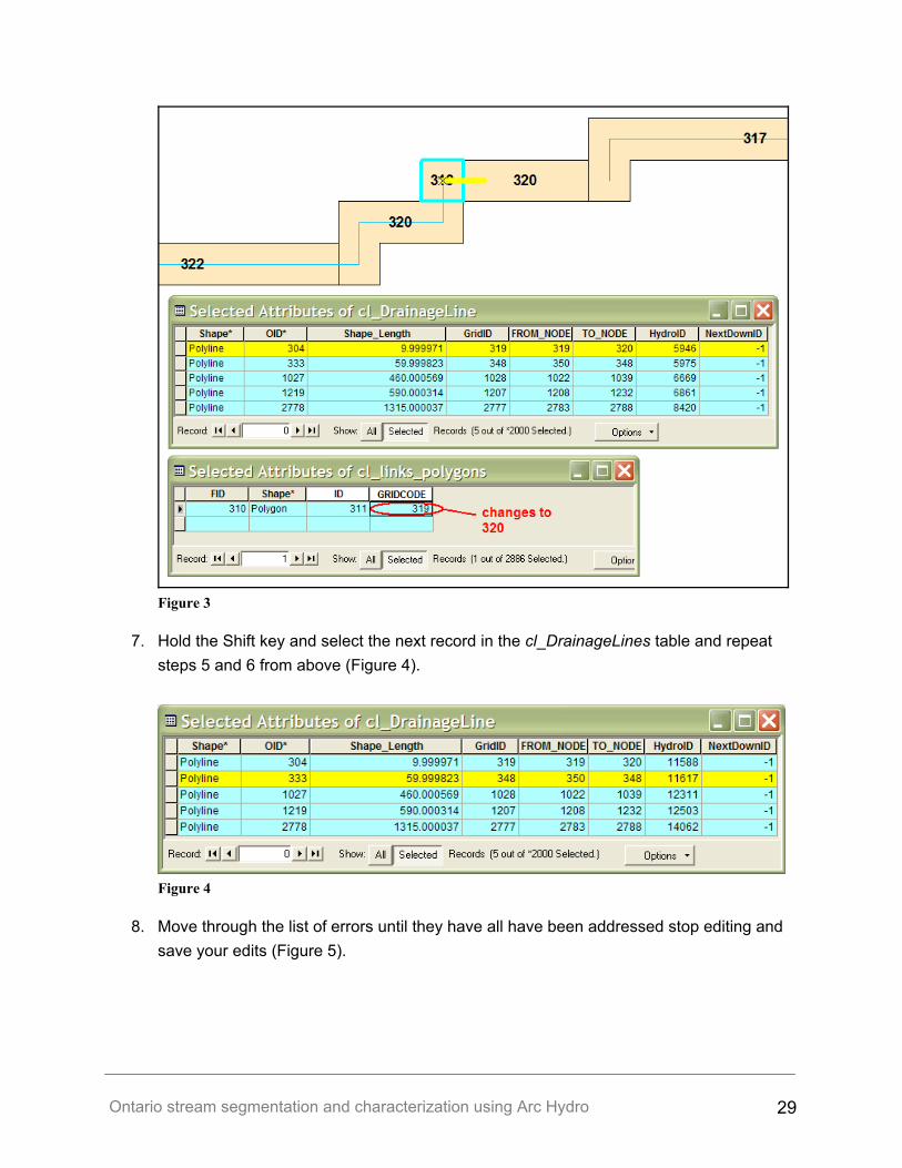
4. Open the cl_DrainageLines table and select the records that have a [NextDownID] = -1 and click the show Selected records only button (Figure 3).
Note: These represent the lines were single cells have disrupted the continuity of flow. The [GridID] values of these single cells must be adjusted to restore continuous flow to the network. 5. Select the first record from the existing then zoom to the currently selected yellow line on
the map while to a scale of between 1:1000 and 1:5000 (Figure 3). 6. Find the single cell that is responsible for the error, select its corresponding polygon in
the cl_links_polygon layer, replace the [GridID] field value in the polygon table with the correct value based on the two adjacent [GridID]s in the cl_links raster (e.g. 319 changes to 320)(Figure 3).
Ontario stream segmentation and characterization using Arc Hydro 29
Figure 3
7. Hold the Shift key and select the next record in the cl_DrainageLines table and repeat steps 5 and 6 from above (Figure 4).
Figure 4
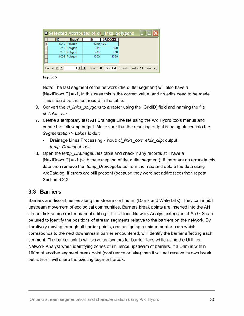
8. Move through the list of errors until they have all have been addressed stop editing and save your edits (Figure 5).
Ontario stream segmentation and characterization using Arc Hydro 30
Figure 5
Note: The last segment of the network (the outlet segment) will also have a [NextDownID] = -1, in this case this is the correct value, and no edits need to be made. This should be the last record in the table. 9. Convert the cl_links_polygons to a raster using the [GridID] field and naming the file
cl_links_corr. 7. Create a temporary test AH Drainage Line file using the Arc Hydro tools menus and
create the following output. Make sure that the resulting output is being placed into the Segmentation > Lakes folder: • Drainage Lines Processing - input: cl_links_corr, efdir_clip; output:
temp_DrainageLines 8. Open the temp_DrainageLines table and check if any records still have a [NextDownID] = -1 (with the exception of the outlet segment). If there are no errors in this data then remove the temp_DrainageLines from the map and delete the data using ArcCatalog. If errors are still present (because they were not addressed) then repeat Section 3.2.3.
3.3 Barriers Barriers are discontinuities along the stream continuum (Dams and Waterfalls). They can inhibit upstream movement of ecological communities. Barriers break points are inserted into the AH stream link source raster manual editing. The Utilities Network Analyst extension of ArcGIS can be used to identify the positions of stream segments relative to the barriers on the network. By iteratively moving through all barrier points, and assigning a unique barrier code which corresponds to the next downstream barrier encountered, will identify the barrier affecting each segment. The barrier points will serve as locators for barrier flags while using the Utilities Network Analyst when identifying zones of influence upstream of barriers. If a Dam is within 100m of another segment break point (confluence or lake) then it will not receive its own break but rather it will share the existing segment break.
Ontario stream segmentation and characterization using Arc Hydro 31
3.3.1 Alignment 1. Open a new ArcMap document and add the efdir_clip raster, the int_efacc raster, the
cl_links_corr raster, the DPoints_preprocessed points, the mnrdams_preprocessed points, and any other Barrier point data that maybe required to the ArcMap TOC.
2. Set the Spatial Analyst Options Settings (see Section 2.4) 3. Save the ArcMap document as barriers.mxd in the Segmentation > Barriers folder. 4. Convert the cl_links_corr raster to vector polygons using the [Value] field without
generalizing the output and naming the file clb_links_polygons. 5. Open the individual Barriers_ {BarrierType} tables and select only the points or lines the
that are required for the analysis (see example below) and export them to new shapefiles naming them Barriers_ {BarrierType}.
Example: The DPoints_preprocessed points contain points for waterfalls, rapids and beaverdams. In this case only the waterfall points would be needed and exported to a new file named Barriers_waterfalls. 6. Add a new field called [B_TYPE] (data type = Text, length = 20) into the
Barriers_{BarrierType} tables. 7. Delete all other fields from Barriers_{BarrierType} tables. 8. Insert (calculate) a text string which identifies the different type of barriers represented by
the points (e.g. MNR Dam, CA Dam, Waterfall etc.) 9. Combine the Barriers_ {BarrierType} points using the Merge tool (Data Management >
General) naming it barriers_merged. 10. Turn off all the other individual Barriers_ {BarrierType} points. 11. Add a new field barriers_merged table called [BarrierID] (data type = long) and calculate
a unique code number with the expression: [FID] + 1 12. Start an edit session and make the barriers_merged the target layer. 13. If the barrier point is within 100m of an existing segment break point then move the point
to centre of the cell just below (downstream) the break line, otherwise move the point into the centre of the stream link polygon at the centre of the nearest cell.
14. Save the edits but keep the edit session open.
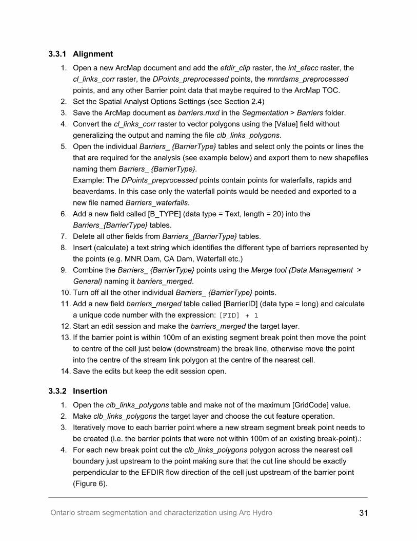
3.3.2 Insertion 1. Open the clb_links_polygons table and make not of the maximum [GridCode] value. 2. Make clb_links_polygons the target layer and choose the cut feature operation. 3. Iteratively move to each barrier point where a new stream segment break point needs to
be created (i.e. the barrier points that were not within 100m of an existing break-point).: 4. For each new break point cut the clb_links_polygons polygon across the nearest cell
boundary just upstream to the point making sure that the cut line should be exactly perpendicular to the EFDIR flow direction of the cell just upstream of the barrier point (Figure 6).
Ontario stream segmentation and characterization using Arc Hydro 32
Figure 6
5. Create a new Unique [GridCode] for the newly created polygon by adding one to the
GridCodemax recorded earlier (i.e. GridCodemax + 1) this new value then replaces the which replaces GridCodemax value for the next new polygon and so on.. Every time a new polygon is created with this method the GridCodemax should be incremented by one to ensure a unique [GridCode] value exists for all polygons.
Example: GridCodemax
= 2821
GridCodemax + 1
= 2822
GridCodemax
= 2822 GridCode
max +1 = 2823 etc.
6. Open the clb_links_polygons table and assign a new unique [GridCode] to the new polygon, upstream of the cut line.
7. Convert the clb_links_polygons to a new raster layer and name the output clb_links. 8. Save the barriers.mxd ArcMAp document and close ArcMap.
Ontario stream segmentation and characterization using Arc Hydro 33
4 Network
4.1 Generation Arc Hydro’s assigns a unique [HydroID] to each spatial entity (e.g. DrainageLine, Catchment etc.) of the geodatabase that leads to and includes the final geometric network. The appropriate internal assignment of HydroIDs and spatial relationships can be disrupted if individual components of the geodatabase are deleted and recreated. To prevent this from happening do not delete individual component of the geodatabase if a mistake was made. Delete the entire geodatabase and start from the very beginning of Section 4.1.
1. Save all documents and restart the computer. 2. Open a new ArcMap document and add the efdir_clip raster, the int_efacc raster, the
clb_links raster to the ArcMap TOC. 3. Set the Spatial Analyst Options Settings (see Section 2.4) 4. Save the ArcMap document as clb_network.mxd in the Segmentation > Networking
folder. 5. Using the Arc Hydro menus create the following output. Make sure that the resulting
output is being placed into the Segmentation > Networking folder. Terrain Preprocessing:
• Catchment Grid Delineation - input: efdir_clip, clbnet_links; output: clbnet_Cat • Catchment Polygons Processing - input: clbnet_Cat; output: clbnet_Catchments • Drainage Lines Processing - input: clbnet_links, efdir_clip; output:
clbnet_DrainageLines • Adjoint Catchment Processing - input: clbnet_DrainageLines, clbnet_Catchments;
output: clbnet_AdjointCatchments • Drainage Point Processing - input: int_efacc, clbnet_Cat, clbnet_Catchment; output:
clbnet_DrainagePoint Attribute Tools: • Generate To/From Node for Lines - input: clbnet_DrainageLines Network Tools: • Hydro Network Generation - input: clbnet_DrainageLines, clbnet_Catchment,
clbnet_DrainagePoint; output: clbnet_HydroEdge, clbnet_HydroJunction; Hydro Network Properties: Name: ArcHydro; Snap Tolerance: Default.
• Inspect the new clbnet_HydroJunction points to ensure that all confluences and stream endpoints have an associated junction. In some instances some junction points are assigned to a separate feature class and not the clbnet_HydroJunction points. If this happens save the clb_network.mxd ArcMap document and close ArcMap.
Ontario stream segmentation and characterization using Arc Hydro 34
• Using ArcCatalog delete the following feature classes form the clb_network geodatabase: ArcHydro geometric network, ArcHydro_Junctions points, clbnet_HydroEdge lines, clbnet_HydroJunction points and the clbnetHydroJunctionHasclbnet_Catchment relationship class.
• Close ArcCatalog and open the clb_network.mxd document and remove the now disconnected feature classes from the TOC.
• Repeat the Hydro Network Generation procedure exactly as before and this second iteration of the network should include all the necessary junction points.
6. Save the clb_network.mxd ArcMap document and close ArcMap. 7. Create a back-up copy of entire Networking folder is copied in the Backup_Results
folder.
4.2 Post-processing
4.2.1 Adding Attribute Fields 1. Open a new ArcMap document and add the efdir_clip raster, the clbnet_HydroEdge
lines, and the clb_HydroJunction points (from the clb_network geodatabase) to the ArcMap TOC.
2. Set the Spatial Analyst Options Settings (see Section 2.4). 3. Save the ArcMap document as postprocessing.mxd in the Segmentation >
Postprocessing folder. 4. Add the necessary attribute fields to the clbnet_HydroEdge tables using the AddField
command of ArcGIS command line window. A text file named AddFieldstoHydroEdgeTable.txt is included on the example data CD-ROM in the Scripts folder. This file contain the required automation script which can be cut and pasted into the ArcGIS command line window for execution. The user can add, remove and modify this script to meet the needs of the analysis. For example an additional set of fields could be included to hold data regarding all forest land cover types combined (e.g. [RCA_Forested, [RCA_pForested] etc.)
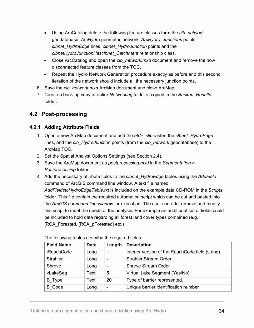
The following tables describe the required fields:
Field Name Data Length Description iReachCode Long - Integer version of the ReachCode field (string) Strahler Long - Strahler Stream Order Shreve Long - Shreve Stream Order vLakeSeg Text 5 Virtual Lake Segment (Yes/No) B_Type Text 20 Type of barrier represented. B_Code Long - Unique barrier identification number
Ontario stream segmentation and characterization using Arc Hydro 35
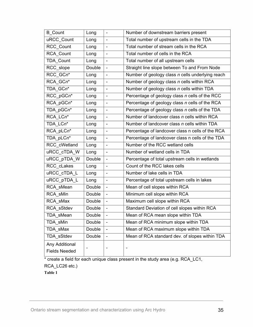
B_Count Long - Number of downstream barriers present uRCC_Count Long - Total number of upstream cells in the TDA RCC_Count Long - Total number of stream cells in the RCA RCA_Count Long - Total number of cells in the RCA TDA_Count Long - Total number of all upstream cells RCC_slope Double - Straight line slope between To and From Node RCC_GCn* Long - Number of geology class n cells underlying reach RCA_GCn* Long - Number of geology class n cells within RCA TDA_GCn* Long - Number of geology class n cells within TDA RCC_pGCn* Long - Percentage of geology class n cells of the RCC RCA_pGCn* Long - Percentage of geology class n cells of the RCA TDA_pGCn* Long - Percentage of geology class n cells of the TDA RCA_LCn* Long - Number of landcover class n cells within RCA TDA_LCn* Long - Number of landcover class n cells within TDA RCA_pLCn* Long - Percentage of landcover class n cells of the RCA TDA_pLCn* Long - Percentage of landcover class n cells of the TDA RCC_cWetland Long - Number of the RCC wetland cells uRCC_cTDA_W Long - Number of wetland cells in TDA uRCC_pTDA_W Double - Percentage of total upstream cells in wetlands RCC_cLakes Long - Count of the RCC lakes cells uRCC_cTDA_L Long - Number of lake cells in TDA uRCC_pTDA_L Long - Percentage of total upstream cells in lakes RCA_sMean Double - Mean of cell slopes within RCA RCA_sMin Double - Minimum cell slope within RCA RCA_sMax Double - Maximum cell slope within RCA RCA_sStdev Double - Standard Deviation of cell slopes within RCA TDA_sMean Double - Mean of RCA mean slope within TDA TDA_sMin Double - Mean of RCA minimum slope within TDA TDA_sMax Double - Mean of RCA maximum slope within TDA TDA_sStdev Double - Mean of RCA standard dev. of slopes within TDA
Any Additional Fields Needed
- - -
* create a field for each unique class present in the study area (e.g. RCA_LC1, RCA_LC26 etc.)
Table 1
Ontario stream segmentation and characterization using Arc Hydro 36
5. Start and edit session with the clbnet_HydroEdges as the target and calculate the integer type [iReachCode] field to equal the text type [ReachCode] field of the clbnet_HydroEdge table.
6. Open the clbnet_HydroJunction table and manually add these four fields: • [C_TYPE] data type: text, length: 20 • [Main_FACC] data type: long integer • [Trib_FACC] data type: long integer • [CSR] data type: double
4.2.2 Identifying Virtual Lake Segments 1. Add the bndclean raster (from Section 3.2.1 ) to the TOC. 2. Convert the bndclean raster to a vector polygon using the Raster to Feature function
(Spatial Analyst Menu > Convert) with bndclean raster as the input, the [Value] field as the field, the Output geometry type as Polygon and Generalize Lines unchecked and naming the output vectorized_bndcln_lakes.
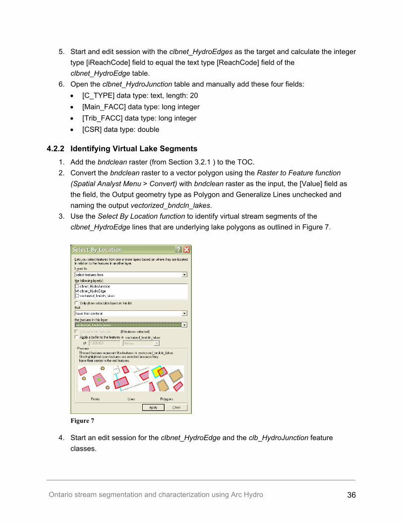
3. Use the Select By Location function to identify virtual stream segments of the clbnet_HydroEdge lines that are underlying lake polygons as outlined in Figure 7.
Figure 7
4. Start an edit session for the clbnet_HydroEdge and the clb_HydroJunction feature classes.

Ontario stream segmentation and characterization using Arc Hydro 37
5. For the selected records of the clbnet_HydroEdge table calculate a value of “YES” for the [VLakeSeg] field then reverse the selection and calculate a value of “NO” for the reversed selection..
4.2.3 Identifying Virtual Lake Confluences and Lake Outlets 1. Use the Select By Location function to identify virtual junctions of the clb_HydroJunction
points that are underlying lake polygons as outlined in Figure 8 and calculate a value of “Virtual Lake” for the [C_TYPE] field.
Figure 8
6. Open the clb_HydroJunction table and use the Select By Attribute function to select all records where the [C_TYPE] field is NOT NULL (<>) and then invert the selection.
7. Select from the current selection (create a sub-set) where the [SchemaRole] field is equal to one and calculate a value of “Lake Outlet” for the [C_TYPE] field for the selected records.
8. Stop editing and save the edits.
4.2.4 Transferring Confluence Information 1. Add the confluence_information_transfer point shapefile to the TOC. 2. Perform a spatial join as outlined in Figure 9 to create a new point shapefile named
spatially_joined_HydroJunctions_CSR_transfer.
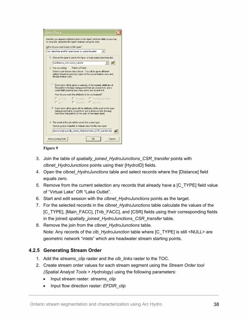
Ontario stream segmentation and characterization using Arc Hydro 38
Figure 9
3. Join the table of spatially_joined_HydroJunctions_CSR_transfer points with
clbnet_HydroJunctions points using their [HydroID] fields. 4. Open the clbnet_HydroJunctions table and select records where the [Distance] field
equals zero. 5. Remove from the current selection any records that already have a [C_TYPE] field value
of “Virtual Lake” OR “Lake Outlet”. 6. Start and edit session with the clbnet_HydroJunctions points as the target. 7. For the selected records in the clbnet_HydroJunctions table calculate the values of the
[C_TYPE], [Main_FACC], [Trib_FACC], and [CSR] fields using their corresponding fields in the joined spatially_joined_HydroJunctions_CSR_transfer table.
8. Remove the join from the clbnet_HydroJunctions table. Note: Any records of the clb_HydroJunction table where [C_TYPE] is still <NULL> are geometric network “inlets” which are headwater stream starting points.
4.2.5 Generating Stream Order 1. Add the streams_clip raster and the clb_links raster to the TOC. 2. Create stream order values for each stream segment using the Stream Order tool
(Spatial Analyst Tools > Hydrology) using the following parameters: • Input stream raster: streams_clip • Input flow direction raster: EFDIR_clip
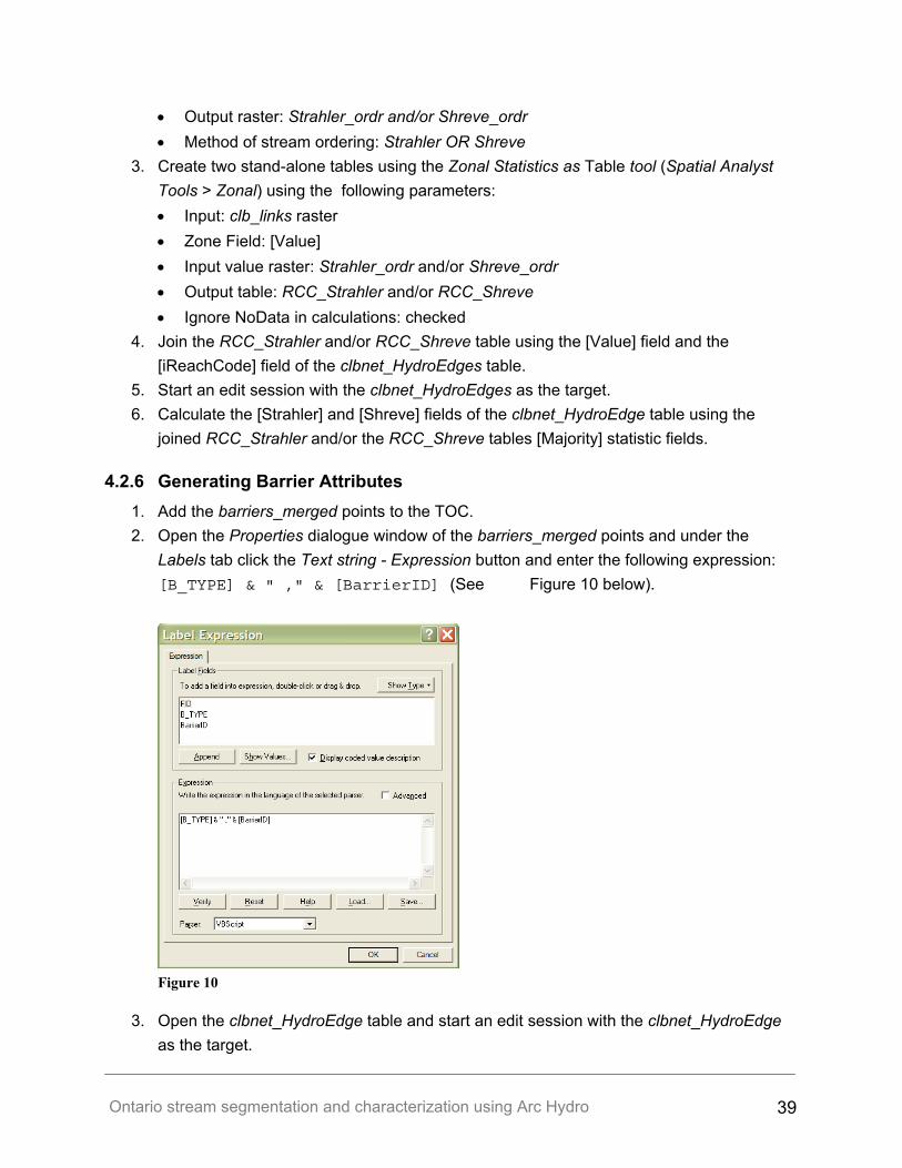
Ontario stream segmentation and characterization using Arc Hydro 39
• Output raster: Strahler_ordr and/or Shreve_ordr • Method of stream ordering: Strahler OR Shreve
3. Create two stand-alone tables using the Zonal Statistics as Table tool (Spatial Analyst Tools > Zonal) using the following parameters: • Input: clb_links raster • Zone Field: [Value] • Input value raster: Strahler_ordr and/or Shreve_ordr • Output table: RCC_Strahler and/or RCC_Shreve • Ignore NoData in calculations: checked
4. Join the RCC_Strahler and/or RCC_Shreve table using the [Value] field and the [iReachCode] field of the clbnet_HydroEdges table.
5. Start an edit session with the clbnet_HydroEdges as the target. 6. Calculate the [Strahler] and [Shreve] fields of the clbnet_HydroEdge table using the
joined RCC_Strahler and/or the RCC_Shreve tables [Majority] statistic fields.
4.2.6 Generating Barrier Attributes 1. Add the barriers_merged points to the TOC. 2. Open the Properties dialogue window of the barriers_merged points and under the
Labels tab click the Text string - Expression button and enter the following expression: [B_TYPE] & " ," & [BarrierID] (See Figure 10 below).
Figure 10
3. Open the clbnet_HydroEdge table and start an edit session with the clbnet_HydroEdge as the target.
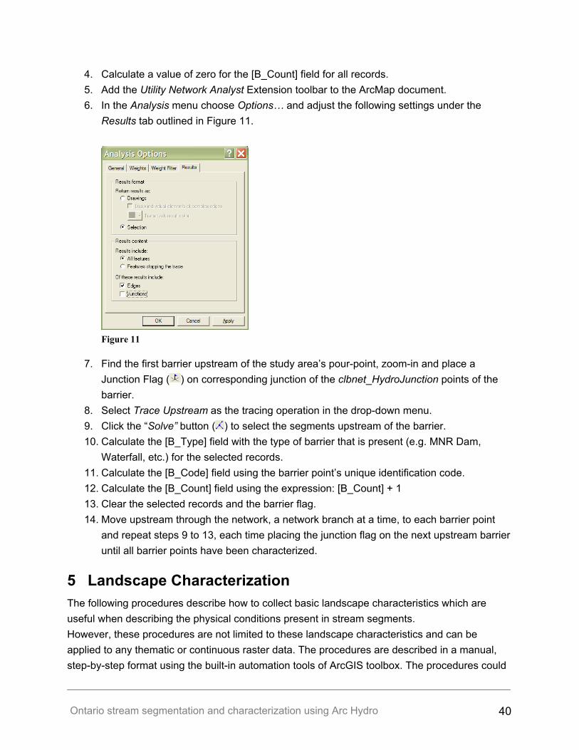
Ontario stream segmentation and characterization using Arc Hydro 40
4. Calculate a value of zero for the [B_Count] field for all records. 5. Add the Utility Network Analyst Extension toolbar to the ArcMap document. 6. In the Analysis menu choose Options… and adjust the following settings under the
Results tab outlined in Figure 11.
Figure 11
7. Find the first barrier upstream of the study area’s pour-point, zoom-in and place a Junction Flag ( ) on corresponding junction of the clbnet_HydroJunction points of the barrier.
8. Select Trace Upstream as the tracing operation in the drop-down menu. 9. Click the “Solve” button ( ) to select the segments upstream of the barrier. 10. Calculate the [B_Type] field with the type of barrier that is present (e.g. MNR Dam,
Waterfall, etc.) for the selected records. 11. Calculate the [B_Code] field using the barrier point’s unique identification code. 12. Calculate the [B_Count] field using the expression: [B_Count] + 1 13. Clear the selected records and the barrier flag. 14. Move upstream through the network, a network branch at a time, to each barrier point
and repeat steps 9 to 13, each time placing the junction flag on the next upstream barrier until all barrier points have been characterized.
5 Landscape Characterization The following procedures describe how to collect basic landscape characteristics which are useful when describing the physical conditions present in stream segments. However, these procedures are not limited to these landscape characteristics and can be applied to any thematic or continuous raster data. The procedures are described in a manual, step-by-step format using the built-in automation tools of ArcGIS toolbox. The procedures could
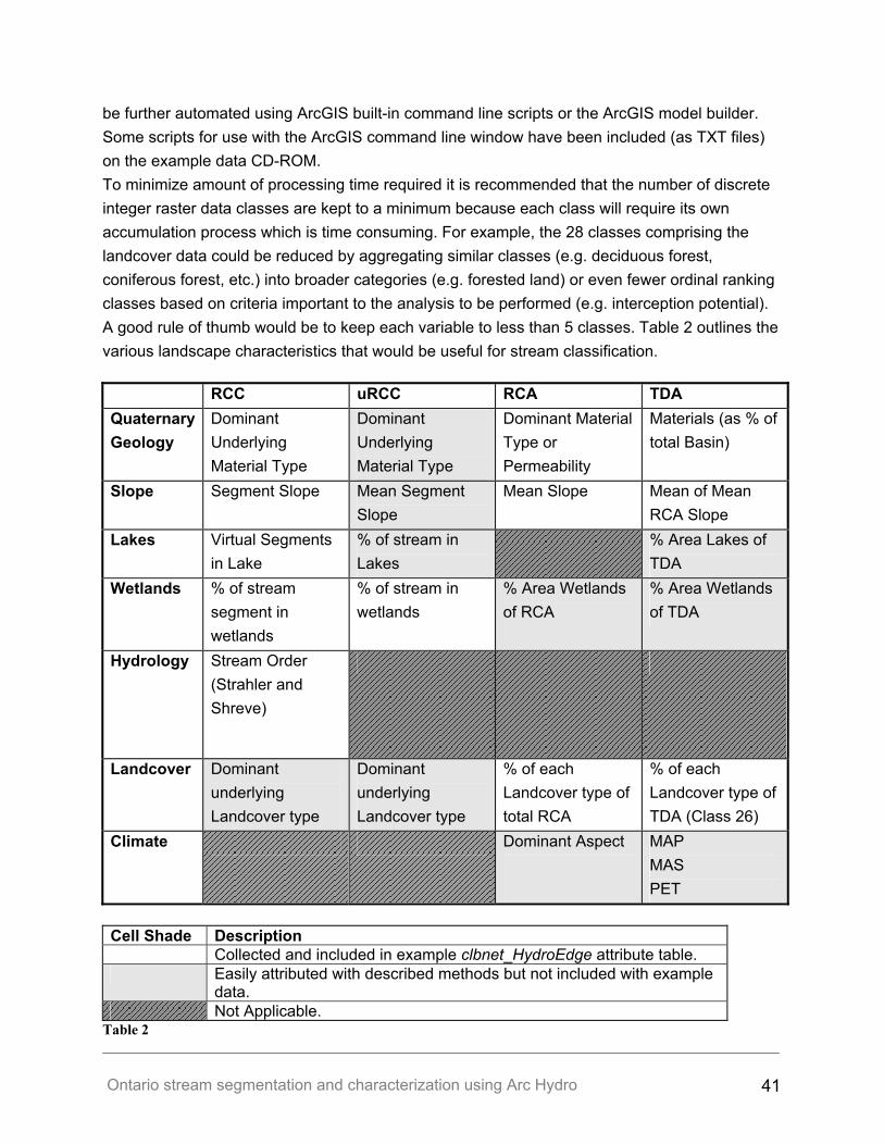
Ontario stream segmentation and characterization using Arc Hydro 41
be further automated using ArcGIS built-in command line scripts or the ArcGIS model builder. Some scripts for use with the ArcGIS command line window have been included (as TXT files) on the example data CD-ROM. To minimize amount of processing time required it is recommended that the number of discrete integer raster data classes are kept to a minimum because each class will require its own accumulation process which is time consuming. For example, the 28 classes comprising the landcover data could be reduced by aggregating similar classes (e.g. deciduous forest, coniferous forest, etc.) into broader categories (e.g. forested land) or even fewer ordinal ranking classes based on criteria important to the analysis to be performed (e.g. interception potential). A good rule of thumb would be to keep each variable to less than 5 classes. Table 2 outlines the various landscape characteristics that would be useful for stream classification. RCC uRCC RCA TDA Quaternary Geology
Dominant Underlying Material Type
Dominant Underlying Material Type
Dominant Material Type or Permeability
Materials (as % of total Basin)
Slope Segment Slope Mean Segment Slope
Mean Slope Mean of Mean RCA Slope
Lakes Virtual Segments in Lake
% of stream in Lakes
% Area Lakes of TDA
Wetlands % of stream segment in wetlands
% of stream in wetlands
% Area Wetlands of RCA
% Area Wetlands of TDA
Hydrology Stream Order (Strahler and Shreve)
Landcover Dominant underlying Landcover type
Dominant underlying Landcover type
% of each Landcover type of total RCA
% of each Landcover type of TDA (Class 26)
Climate Dominant Aspect MAP MAS PET
Cell Shade Description Collected and included in example clbnet_HydroEdge attribute table. Easily attributed with described methods but not included with example
data. Not Applicable.
Table 2
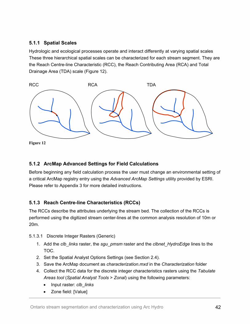
Ontario stream segmentation and characterization using Arc Hydro 42
5.1.1 Spatial Scales Hydrologic and ecological processes operate and interact differently at varying spatial scales These three hierarchical spatial scales can be characterized for each stream segment. They are the Reach Centre-line Characteristic (RCC), the Reach Contributing Area (RCA) and Total Drainage Area (TDA) scale (Figure 12). RCC RCA TDA
Figure 12
5.1.2 ArcMap Advanced Settings for Field Calculations Before beginning any field calculation process the user must change an environmental setting of a critical ArcMap registry entry using the Advanced ArcMap Settings utility provided by ESRI. Please refer to Appendix 3 for more detailed instructions.
5.1.3 Reach Centre-line Characteristics (RCCs) The RCCs describe the attributes underlying the stream bed. The collection of the RCCs is performed using the digitized stream center-lines at the common analysis resolution of 10m or 20m.
5.1.3.1 Discrete Integer Rasters (Generic)
1. Add the clb_links raster, the sgu_pmsm raster and the clbnet_HydroEdge lines to the TOC.
2. Set the Spatial Analyst Options Settings (see Section 2.4). 3. Save the ArcMap document as characterization.mxd in the Characterization folder 4. Collect the RCC data for the discrete integer characteristics rasters using the Tabulate
Areas tool (Spatial Analyst Tools > Zonal) using the following parameters: • Input raster: clb_links • Zone field: [Value]
Ontario stream segmentation and characterization using Arc Hydro 43
• Input raster or feature class data: {discrete integer raster name} • Class field: [Value] • Output table: RCC_{discrete integer raster name} • Processing cell size: matching EFDIR raster cell size
5. Collect the RCC data for the discrete integer characteristics rasters using the Zonal Statistics as Table tool (Spatial Analyst Tools > Zonal) using the following parameters: • Input raster: clb_links • Zone field: [Value] • Input raster or feature class data: {discrete integer raster name} • Class field: [Value] • Output table: RCC_{discrete integer raster name}_count • Ignore NoData in calculations: checked
6. Join the RCC_{discrete integer raster name}_count table using the [Value] field and the [GridID] field of the table.
7. Calculate the [RCC_Count] field of the clbnet_HydroEdge table using the [Count] field of the RCC_{discrete integer raster name}_count stand-alone table.
8. Remove the current join from the clbnet_HydroEdge table. 9. Join the RCC_{discrete integer raster name} table using the [Value] field and the
[GridID] field of the table. 10. Calculate the [RCC_{discrete integer raster class}] field of the clbnet_HydroEdge using
the corresponding class field of the joined RCC_{discrete integer raster name} stand alone table.
5.1.3.2 Slope
1. Add the xgrid raster, the ygrid raster, the hillshade raster and the dem_clip raster to the TOC.
2. Create three zonal statistics tables which will describe the Δx, Δy, and Δz using the Statistics as Table tool (Spatial Analyst Tools > Zonal) with the following parameters: • Input: clb_links raster • Zone Field: [Value] • Input value raster: xGrid / yGrid / DEM_clip • Output table: RCC_X / RCC_Y / RCC_Z • Ignore NoData in calculations: checked
3. Add a new field called [calcRCCslope] (data type: double) to the RCC_X stand-alone table.
4. Join both the RCC_Y and RCC_Z stand-alone tables to the RCC_X stand-alone table using the [Value] fields.
Ontario stream segmentation and characterization using Arc Hydro 44
5. Calculate the [calcRCCslope] field of the RCC_X stand-alone table using the following VBA expression in the Advanced Window of the Field Calculator and set the field to equal the variable slope (i.e. [calcRCCslope] = slope).
dim a2 as long dim b2 as long dim c as double dim slope as double if [RCC_Z.RANGE] = 0 then slope = 0 else a2 = [RCC_X.RANGE] ^ 2 b2 = [RCC_Y.RANGE] ^ 2 c = Sqr(a2 + b2) slope = [RCC_Z.RANGE] / c endif
6. Remove all Joins from the RCC_X stand alone table. 7. Join the clbnet_HydroEdge table to the RCC_X stand-alone table using the [GridID] field
of the clbnet_HydroEdge table and the [Value] field of the RCC_X stand-alone table. 8. Calculate the [RCC_slope] field of the clbnet_HydroEdge table to equal the
[calcRCCslope] field of the RCC_X stand-alone table.
5.1.3.3 Stream Length in Lakes and Wetlands (or any Integer Class Zone)
1. Collect the RCC data for the discrete integer characteristics rasters using the Tabulate Areas tool (Spatial Analyst Tools > Zonal) using the following parameters: • Input raster: clb_links • Zone field: [Value] • Input raster or feature class data: Landcover28{2000} • Class field: [Value] • Output table: RCC_Landcover28{2000} • Processing cell size: matching EFDIR raster cell size
2. Join the RCC_Landcover28{2000} table to the clbnet_HydroEdge table using the [Value] and [GridID] fields of the tables and start and edit session with the clbnet_HydroEdge lines as the target layer.
3. Calculate the [RCC_cLakes] and the [RCC_cWetland] fields of the clbnet_HydroEdge table using the joined RCC_Landcover28{2000} table and the following expressions:
[RCC_cLakes]=RCC_Landcover28.[Value_1] [RCC_cWetland]=Sum(RCC_Landcover28.[Value{RCC_WetlandClasses}]
Example: [RCC_landcover28.VALUE_5] + [RCC_landcover28.VALUE_6] + RCC_landcover28.VALUE_7] + [RCC_landcover28.VALUE_8]

Ontario stream segmentation and characterization using Arc Hydro 45
5.1.4 Reach Contributing Areas (RCAs) The RCAs describe the landscape attribute composition of the local landscape draining to each individual reach segment. The names of the data layers in the following methods have been kept generic to emphasize that any raster data to be used. For a list of attributes (fields) required for this report please refer to Table 1 in Section 4.2.1.
5.1.4.1 Discrete Integer Rasters (Generic)
1. Add the clbnet_Cat raster to the TOC. 2. Collect the RCA data for the discrete integer characteristics rasters using the Tabulate
Areas tool (Spatial Analyst Tools > Zonal) using the following parameters: • Input raster: clb_Cat raster • Zone field: [Value] • Input raster or feature class data: {discrete integer raster name} • Class field: [Value] • Output table: RCA_{discrete integer raster name} • Processing cell size: matching EFDIR raster cell size
3. Collect the RCC data for the discrete integer characteristics rasters using the Zonal Statistics as Table tool (Spatial Analyst Tools > Zonal) using the following parameters: • Input raster: clbnet_Cat raster • Zone field: [Value] • Input raster or feature class data: {discrete integer raster name} • Class field: [Value] • Output table: RCA_{discrete integer raster name}_count • Ignore NoData in calculations: checked
4. Join the RCA_{discrete integer raster name}_count stand alone table to the clbnet_HydroEdge table using the [GridID] field and the [Value] field and start and edit session with the clbnet_HydroEdge lines as the target layer.
5. Calculate the [RCA_Count] field of the clbnet_HydroEdge table using the [Count] field of the RCA_{discrete integer raster name}_count joined table.
6. Remove the current join from the clbnet_HydroEdge table. 7. Join the RCA_{ discrete integer raster name } table using the [Value] field and the
[GridID] field of the table. 8. Calculate the [RCA_{discrete integer raster class}] field of the clbnet_HydroEdge using
the corresponding class field of the joined RCA_{discrete integer raster name} stand alone table.
5.1.4.2 Floating Point Rasters (Generic)
1. Add the slope raster to the TOC.
Ontario stream segmentation and characterization using Arc Hydro 46
2. Collect the RCA data for the continuous floating point characteristics rasters using the Zonal Statistics as Table tool (Spatial Analyst Tools > Zonal) using the following parameters: • Input raster: clbnet_Cat raster • Zone Field: [Value] • Input value raster: {floating point raster name} • Output table: RCA_{floating point raster name} • Ignore NoData in calculations: checked
3. Join the RCA_{floating point name} table using the [Value] and [GridID] fields of the tables and start and edit session with the clbnet_HydroEdge lines as the target layer.
4. Calculate the [RCA_{ZonalStatistic}] field of the clbnet_HydroEdge table using the [RCA_{statistictype}] zonal statistics fields.
5.1.5 Total Drainage Areas (TDAs) The TDAs describe the landscape attribute composition of each segment’s total upstream drainage area in percent of total drainage area. In order to characterize the segments at the TDA scale each attribute class must be accumulated as a separate process using the previously collected RCA attributes. The accumulate function will sum all the upstream occurrences of an attribute class and write them back to the processing segment in the clbnet_DrainageLine table. The accumulation is highly processing intensive since each segments upstream RCCs and/or RCAs must be identified and their values summed or averaged for each attribute class. This will take a considerable amount of time (several hours for each attribute). Keep in mind that thousands of upstream areas are identified and accumulated for thousands of segments. It should be noted that the accumulation process works faster if there are fewer fields in the accumulation feature class table. It is therefore recommended that only the immediate accumulation source and target fields be added to this attribute table. Once the accumulation is completed the values of the target field should be transferred to the clbnet_HydroEdge table. For added data security export the clbnet_DrainageLine table to the Backup_Results > Tables folder. The source and target fields in the clbnet_DrainageLine table can then be deleted and replaced with the next source and target field.
5.1.5.1 Total Drainage Area
1. Add both the required Target and Source field to the clbnet_DrainageLine table (see Table 1 in Section 4.2.1 for data types).
2. Run an AH accumulation process (AH Attribute Tools) on the clbnet_DrainageLine lines using the following settings: • Trace Type: Feature Layer with NextDownID: clbnet_DrainageLine Next Down ID Field: [NextDownID]
Ontario stream segmentation and characterization using Arc Hydro 47
Use selected features only: unchecked • Source for Accumulation: Source Feature Layer: clbnet_DrainageLine Source Field: [RCA_Count] • Accumulation Type: Option: Sum • Target for Accumulation: Target Feature Layer: clbnet_DrainageLine Target Field: [TDA_Count]
3. Join the clbnet_DrainageLine and the clbnet_HydroEdge tables using the [GridID] and the [iReachCode] field respectively.
4. Transfer the accumulation results from the clbnet_DrainageLine table to the clbnet_HydroEdge table by calculating the field in the clbnet_HydroEdge table with its corresponding value in the joined clbnet_DrainageLine table.
5. Open the clbnet_DrainageLine and export it to the Backup_Results > Tables folder naming it Accumulation_Backup_{AccumulationTargetFieldName} (e.g. Accumulation_Backup_TDA_Count.dbf).
6. Remove the table join from the clbnet_HydroEdge table and delete the Accumulation Source and Target fields from the clbnet_DrainageLine table.
5.1.5.2 Discrete Integer Rasters (Generic)
1. Add both the required Target and Source field to the clbnet_DrainageLine table (see Table 1 in Section 4.2.1 for data types).
2. Run an accumulation on the clbnet_DrainageLine lines using the following settings once for each of the [RCA_{attribute}] fields of the clbnet_DrainageLine table: • Trace Type: Feature Layer with NextDownID: clbnet_DrainageLine Next Down ID Field: [NextDownID] Use selected features only: unchecked • Source for Accumulation: Source Feature Layer: clbnet_DrainageLine Source Field: [RCA_{integer_attribute}] • Accumulation Type: Option: Sum • Target for Accumulation: Target Feature Layer: clbnet_DrainageLine Target Field: [TDA_{integer_attribute}]
3. Join the clbnet_DrainageLine and the clbnet_HydroEdge tables using the [GridID] and the [iReachCode] field respectively.
Ontario stream segmentation and characterization using Arc Hydro 48
4. Transfer the accumulation results from the clbnet_DrainageLine table to the clbnet_HydroEdge table by calculating the field in the clbnet_HydroEdge table with its corresponding value in the joined clbnet_DrainageLine table.
5. Open the clbnet_DrainageLine and export it to the Backup_Results > Tables folder naming it Accumulation_Backup_{AccumulationTargetFieldName} (e.g. Accumulation_Backup_TDA_Count.dbf).
6. Remove the table join from the clbnet_HydroEdge table and delete the Accumulation Source and Target fields from the clbnet_DrainageLine table.
5.1.5.3 Floating Point Rasters (Generic)
1. Add both the required Target and Source field to the clbnet_DrainageLine table (see Table 1 in Section 4.2.1 for data types).
2. Run an accumulation on the clbnet_DrainageLine lines using the following settings once for each of the [RCA_{attribute}] fields of the clbnet_DrainageLine table: • Trace Type: Feature Layer with NextDownID: clbHydroEdge Next Down ID Field: [NextDownID] Use selected features only: unchecked • Source for Accumulation: Source Feature Layer: clbnet_HydroEdge Source Field: [RCA_{floatingpoint_attribute}] • Accumulation Type: Option: Mean • Target for Accumulation: Target Feature Layer: clbnet_HydroEdge Target Field: [TDA_{floatingpoint _attribute}]
3. Join the clbnet_DrainageLine and the clbnet_HydroEdge tables using the [GridID] and the [iReachCode] field respectively.
4. Transfer the accumulation results from the clbnet_DrainageLine table to the clbnet_HydroEdge table by calculating the field in the clbnet_HydroEdge table with its corresponding value in the joined clbnet_DrainageLine table.
5. Open the clbnet_DrainageLine and export it to the Backup_Results > Tables folder naming it Accumulation_Backup_{AccumulationTargetFieldName} (e.g. Accumulation_Backup_TDA_Count.dbf).
6. Remove the table join from the clbnet_HydroEdge table and delete the Accumulation Source and Target fields from the clbnet_DrainageLine table.
Ontario stream segmentation and characterization using Arc Hydro 49
5.1.5.4 Stream Length in Lakes and Wetlands
1. Add both the required Target and Source field to the clbnet_DrainageLine table (see Table 1 in Section 4.2.1 for data types).
2. Run the following accumulation four times using the same settings each time but substituting in the four different source/target fields of the clbnet_DrainageLine table: • Trace Type: Feature Layer with NextDownID: clbnet_DrainageLine Next Down ID Field: [NextDownID] Use selected features only: unchecked • Source for Accumulation: Source Feature Layer: clbnet_DrainageLine Source Field: [RCC_Count] / [RCC_cLakes] / [uRCC_Wetland] • Accumulation Type: Option: Sum • Target for Accumulation: Target Feature Layer: clbnet_DrainageLine Target Field: [uRCC_Count] / [uRCC_cTDA_L] / [uRCC_cTDA_W]
3. Join the clbnet_DrainageLine and the clbnet_HydroEdge tables using the [GridID] and the [iReachCode] field respectively.
4. Transfer the accumulation results from the clbnet_DrainageLine table to the clbnet_HydroEdge table by calculating the field in the clbnet_HydroEdge table with its corresponding value in the joined clbnet_DrainageLine table.
5. Open the clbnet_DrainageLine and export it to the Backup_Results > Tables folder naming it Accumulation_Backup_{AccumulationTargetFieldName} (e.g. Accumulation_Backup_TDA_Count.dbf).
6. Remove the table join from the clbnet_HydroEdge table and delete the Accumulation Source and Target fields from the clbnet_DrainageLine table.
5.1.6 Calculating the Percentage Fields 1. Calculate the [RCC_p{discrete integer raster class}] (e.g. [RCC_pGCn], [RCC_pLCn]
etc.) fields of the clbnet_HydroEdge table using the following field calculation expression: [RCC_p{discrete integer raster class}] = [RCC_{discrete integer
raster class}]/[RCC_Count] 2. Calculate the [RCA_p{discrete integer raster class}] (e.g. [RCA_pGCn], [RCA_pLCn])
fields of the clbnet_HydroEdge table using the following field calculation expression: [TDA_p{discrete integer raster class}] [TDA_{discrete integer
raster class}]/[RCA_Count] 3. Calculate the [TDA_p{discrete integer raster class}] (e.g. [TDA_pGCn], [TDA_pLCn])
fields of the clbnet_HydroEdge table using the following field calculation expression:
Ontario stream segmentation and characterization using Arc Hydro 50
TDA_p{discrete integer raster class}] = [TDA_{discrete integer raster class}]/[TDA_Count] 4. Calculate the [uRCC_pTDA_L] and [uRCC_cTDA_W] fields of the clbnet_HydroEdge
table using the following expressions: [uRCC_pTDA_L] = [uRCC_cTDA_L]/[uRCC_Count]
[uRCC_pTDA_W] = [uRCC_cTDA_W]/[uRCC_Count]
Ontario stream segmentation and characterization using Arc Hydro 51
Appendix 1: Map Examples
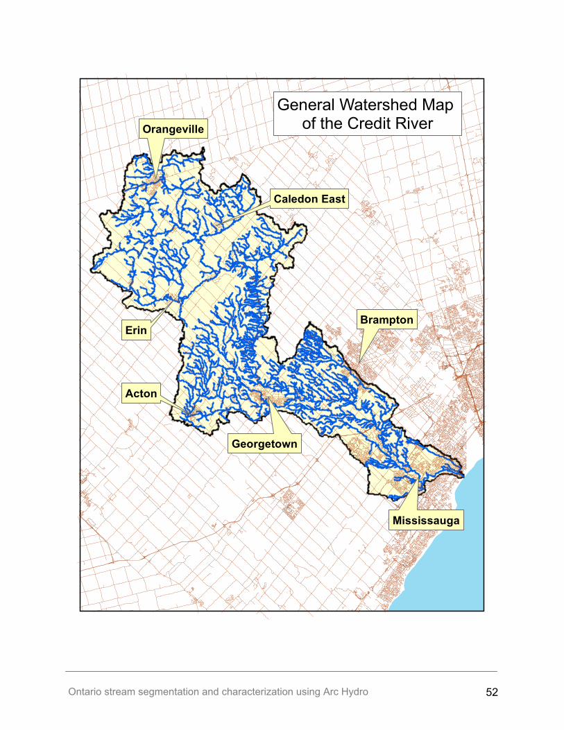
Ontario stream segmentation and characterization using Arc Hydro 52
General Watershed Map of the Credit River
Georgetown
Acton
Orangeville
Mississauga
BramptonErin
Caledon East
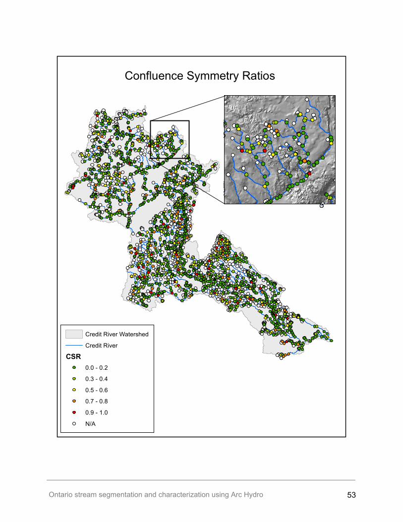
Ontario stream segmentation and characterization using Arc Hydro 53
Confluence Symmetry Ratios
Credit River Watershed
Credit River
CSR0.0 - 0.2
0.3 - 0.4
0.5 - 0.6
0.7 - 0.8
0.9 - 1.0
N/A
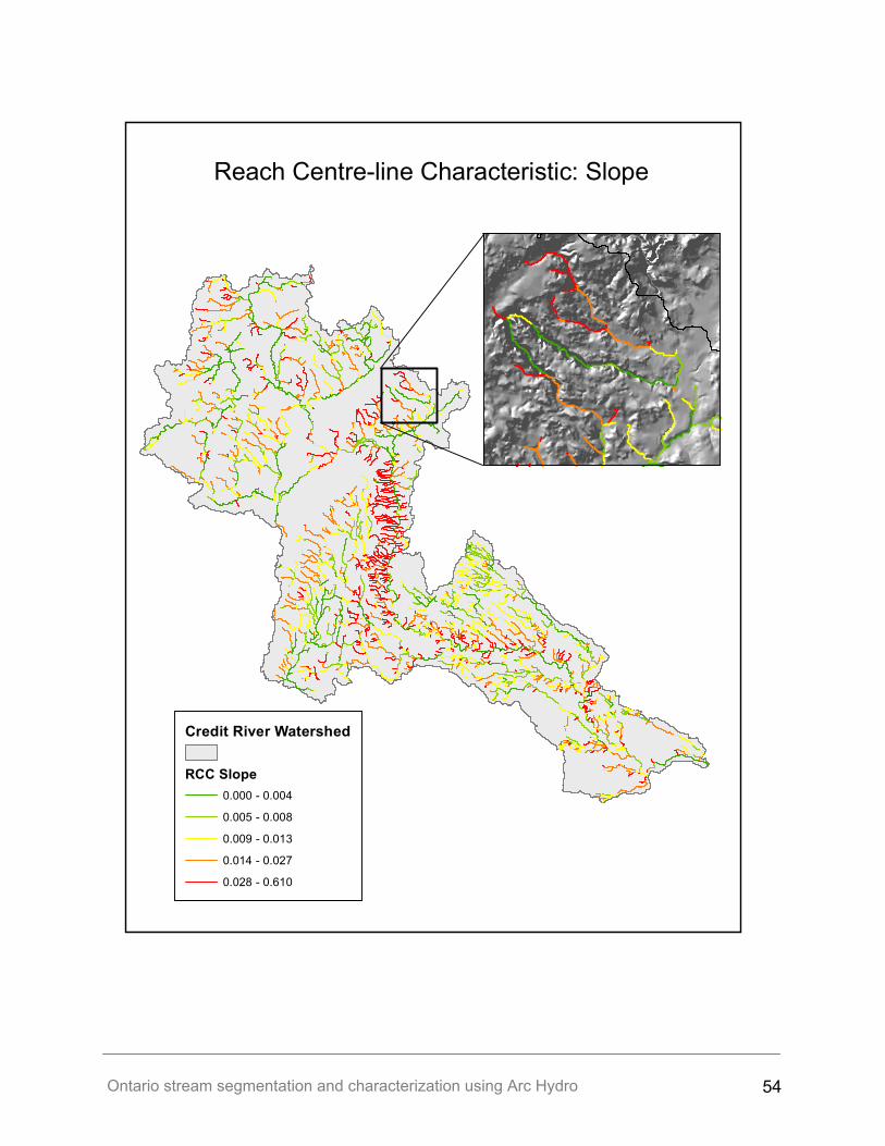
Ontario stream segmentation and characterization using Arc Hydro 54
Reach Centre-line Characteristic: Slope
Credit River Watershed
RCC Slope0.000 - 0.004
0.005 - 0.008
0.009 - 0.013
0.014 - 0.027
0.028 - 0.610
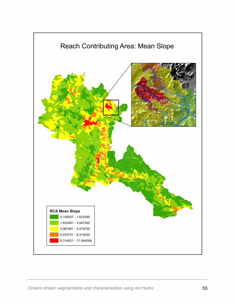
Ontario stream segmentation and characterization using Arc Hydro 55
Reach Contributing Area: Mean Slope
RCA Mean Slope0.145837 - 1.623490
1.623491 - 3.067260
3.067261 - 5.074750
5.074751 - 8.314020
8.314021 - 17.944099
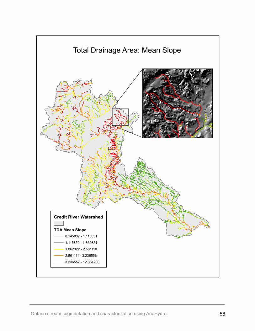
Ontario stream segmentation and characterization using Arc Hydro 56
Total Drainage Area: Mean Slope
Credit River Watershed
TDA Mean Slope0.145837 - 1.115851
1.115852 - 1.862321
1.862322 - 2.561110
2.561111 - 3.236556
3.236557 - 12.384200
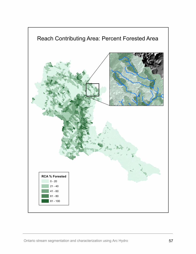
Ontario stream segmentation and characterization using Arc Hydro 57
Reach Contributing Area: Percent Forested Area
RCA % Forested0 - 20
21 - 40
41 - 60
61 - 80
81 - 100
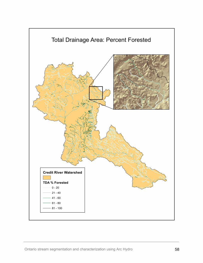
Ontario stream segmentation and characterization using Arc Hydro 58
Total Drainage Area: Percent Forested
Credit River Watershed
TDA % Forested0 - 20
21 - 40
41 - 60
61 - 80
81 - 100
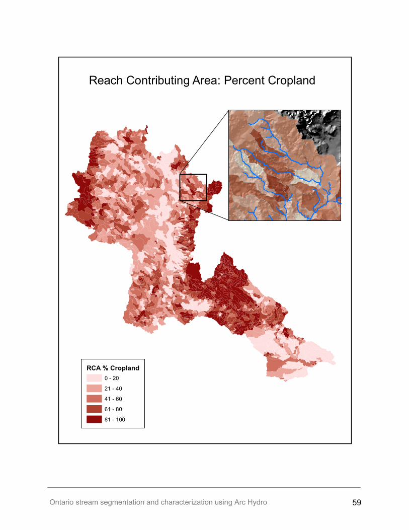
Ontario stream segmentation and characterization using Arc Hydro 59
Reach Contributing Area: Percent Cropland
RCA % Cropland0 - 20
21 - 40
41 - 60
61 - 80
81 - 100
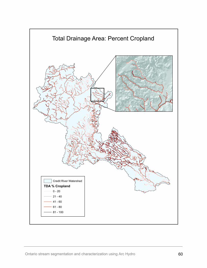
Ontario stream segmentation and characterization using Arc Hydro 60
Total Drainage Area: Percent Cropland
Credit River Watershed
TDA % Cropland0 - 20
21 - 40
41 - 60
61 - 80
81 - 100
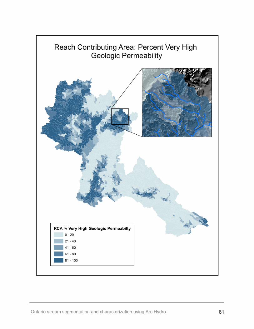
Ontario stream segmentation and characterization using Arc Hydro 61
Reach Contributing Area: Percent Very High Geologic Permeability
RCA % Very High Geologic Permeabilty0 - 20
21 - 40
41 - 60
61 - 80
81 - 100
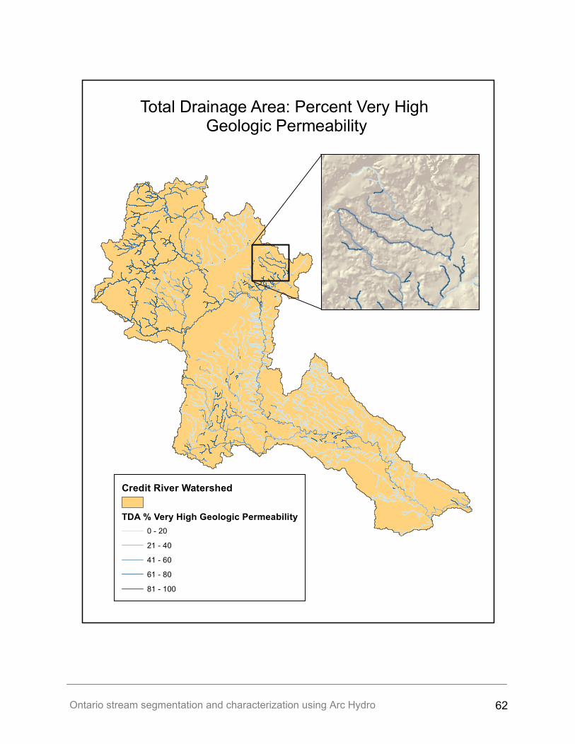
Ontario stream segmentation and characterization using Arc Hydro 62
Total Drainage Area: Percent Very High Geologic Permeability
Credit River Watershed
TDA % Very High Geologic Permeability0 - 20
21 - 40
41 - 60
61 - 80
81 - 100
Ontario stream segmentation and characterization using Arc Hydro 63
Appendix 2: Data Sources and Descriptions
Ontario stream segmentation and characterization using Arc Hydro 64
Enhanced Flow Direction (EFDIR) raster Type: ESRI Integer Grid Resolution: 10m in southern Ontario, 20m in northern Ontario Available Extent: Coordinate System: Universal Transverse Mercator Map Projection: Transverse Mercator Horizontal Datum: NAD83 Source: Land Information Ontario (LIO) Description: The Enhanced Flow Direction Grid is a grid representing surface flow directions derived from Version 2.0 Digital Elevation Model (DEM) with the added enhancement of having the photogrammetrically mapped hydrology (WRIP Water Virtual Flow and NRVIS water body segment) embedded within the grid so that known hydrology is accurately represented within the grid. Because this is based from the version 2 DEM, the Enhanced Flow Direction Grid is referred to as EFDIR2. Also included in version 2 is an alternative assignment of flow direction to shoreline areas. The inclusion has the following effects: Brings the limit of the Flow Direction grid closer to the shoreline resulting in a cleaner product; Allows for the delineation of distinct shoreline catchments not possible in the previous EFD product; Minimizes effects of shoreline bleeding (erroneous catchments being formed in ‘no-data’ areas usually upstream of project areas); and Assigns proper flow directions to minor bays and inlets. To cover Ontario the grid has been divided into 16 pieces, existing in their respective UTM zones 15, 16, 17, and 18. Each grid covers major watersheds within these zones. The naming conventions of the grid follow the naming conventions of the Secondary and Tertiary Provincial watershed layers. The resolution of the Enhanced Flow Direction Grid is the same as the Provincial Digital Elevation Model - 10m for southern Ontario (where 1:10,000 base data exists) and 20m for Northern Ontario (where 1:20,000 base data exists). Currently, nine of the 16 grids which cover south western and eastern Ontario are included in the package. There are index shapefiles included within the package to show the extent of each grid. The requirement to digitally delineate accurate watershed boundaries is a routine task necessary in numerous natural science disciplines. The Provincial Enhanced Flow Direction grid is designed for this purpose. Embedded in the enhanced flow direction grid are three commonly used layers in developing watershed divides; 1) flow directed stream network, 2) lakes and other water bodies, and 3) interpreted flow directions from a digital elevation model. A normal flow direction grid is derived solely from a digital elevation model where flow directions are determined by examining grid elevation values surrounding any one cell, and assigning the flow direction to the steepest down slope neighbour. The enhancement in the provincial enhanced flow direction grid is the inclusion of photogrammetrically mapped, flow directed hydrology, or known hydrology, which forces the derived watershed boundaries to honour (OLID).
Ontario stream segmentation and characterization using Arc Hydro 65
Enhanced Flow Direction Streams raster Type: ESRI Integer Grid Resolution: 10m in southern Ontario, 20m in northern Ontario Available Extent: Coordinate System: Universal Transverse Mercator Map Projection: Transverse Mercator Horizontal Datum: NAD83 Source: Land Information Ontario (LIO) Description: This grid is the raster version of the NRVIS Water Virtual Flow Lines. The streams represented by the cells correspond perfectly with these flow lines. This eliminates the need to use a threshold to extract the streams and therefore the stream network is reproduced exactly in the raster environment.
Provincial Digital Elevation Model (v.2) Type: ESRI floating point raster Resolution: 10m in southern Ontario, 20m in northern Ontario Available Extent: Coordinate System: Universal Transverse Mercator Map Projection: Transverse Mercator Horizontal Datum: NAD83 Vertical Datum: CGD28 - CDN Horizontal Position Accuracy: +/- 10 m (precise) Vertical Position Accuracy: +/- 5 m (reliable) Source: Land Information Ontario (LIO): Digital Elevation Model - Version 2.0.0 - Provincial Tiled Dataset (DEM) Description: Provincial Digital Elevation Model (DEM) Version 2.0.0 is a 3-dimensional raster data set which captures terrain elevations and covers the province of Ontario to the 51st parallel. DEM Version 2.0.0 is an update to the previous DEM Version 1.1.0 dataset. DEM Version 2.0.0 was interpolated using ANUDEM 5.1.0 software and five main elevation datasets: i) OBM-Contour, ii) OBM-DTM, iii) OBM-Spot Height, iv) Water Feature Area (lakes and double-lined rivers), and vi) Water Virtual Flow (stream network). Cell resolutions are 20 metres in northern Ontario and 10 metres in southern Ontario. The DEM has been created by the Water Resources Information Program (WRIP), Geographic Information Branch - Peterborough. There are 150 tiles, in packaged-product format, covering the province. The packages are individually named using the following convention which indicates their extent, version, coordinate system, resolution, and tile number:
Ontario stream segmentation and characterization using Arc Hydro 66
NRVIS Water Area polygons Type: ESRI ArcINFO polygon coverage Scale: 1:10,000 in southern Ontario and 1:20,000 in northern Ontario Available Extent: Coordinate System: Geographic Map Projection: Decimal Degrees Horizontal Datum: NAD83 Source: Land Information Ontario (LIO) Data Class: Waterbody Segment Data Types: Water Area, Permanent (GUT# 1281); Wetland Area, Permanent (GUT# 1800) Description: A Waterbody is a polygon or line feature that identifies a segment of a body of water such as a lake, pond, river, stream, or reservoir. A Waterbody Segment may be the Waterbody in its entirety or a component of the Waterbody. Permanency describes the portion of the year the waterbody segment is inundated by water. Waterbody segments are classified as permanent if they contain water for 9 or more consecutive months under average annual precipitation conditions (taken from Lakes and Rivers Improvement Act Guidelines). Usually these waterbody segments have a defined bed and banks of a permanent nature (OLID). Comments: Waterbodies are received from LIO in MNR District sections. These sections need to be merged together to cover the spatial extent of the entire study area.
NRVIS Water Virtual Flow lines Type: ESRI ArcINFO line coverage Scale: 1:10,000 in southern Ontario and 1:20,000 in northern Ontario Available Extent: see Figure A1-3 Coordinate System: Universal Transverse Mercator Map Projection: Transverse Mercator Horizontal Datum: NAD83 Horizontal Position Accuracy of Features: +/- 10 m (precise) Source: Land Information Ontario (LIO): Water Virtual Flow - Seamless Provincial Data Set Description: The Water Virtual Flow data set is a fully connected, flow directed, stream network with complete topological flow structure. The data was originally based on the Natural Resources Values Information System (NRVIS) Water Body Segment layer and has been updated to create connectivity and flow direction. Streams may also have been edited using information from reliable local sources such as Conservation Authorities and MNR districts. The entire data set has been updated August 2005 incorporating edits received from partners of the Water Resources Information Program. The Water Virtual Flow is divided up into 5 coverages: UTM Zone 15, UTM Zone 16, UTM Zone 17 north, UTM Zone 17 south, and UTM Zone 18. The seamless provincial Water Virtual Flow data layer was part of the original OBM and NRVIS
Ontario stream segmentation and characterization using Arc Hydro 67
database. It has had significant updates from 1998 to 2002 under the Water Resources Information Project (WRIP) and again in August 2005. (OLID)
NRVIS Drainage lines / points Type: ESRI ArcINFO line coverages Scale: 1:10,000 in southern Ontario an 1:20,000 in northern Ontario Available Extent: Coordinate System: Geographic Map Projection: Decimal Degrees Horizontal Datum: NAD83 Vertical Datum: Not Applicable Horizontal Position Accuracy of Features: +/- 10 m (approximate) Horizontal Position Accuracy of Features: +/- 5 m (reliable) Source: Land Information Ontario (LIO) Data Class: Drainage Line / Drainage Point Data Type: Falls - On Double Line River (Line GUT# 51); Falls - On Single Line River (Point GUT# 53) Description: This concrete class corresponds to the OBM feature of the same name. A Drainage Line/Point is a line/point feature that indicates flow or flow obstruction information about a river or stream (OLID).
Surficial Geology of Southern Ontario polygons Type: ESRI polygon shapefile Scale: 1:50,000 – 1:250,000 Available Extent: Coordinate System: Geographic Map Projection: Decimal Degrees Horizontal Datum: NAD83 Vertical Datum: Not Applicable Horizontal Position Accuracy of Features: +/- 250 m (approximate) Source: Ontario Geological Survey – Miscellaneous Release Data 128 (MRD 128) Description: “Ontario Geological Survey (author) The Surficial Geology of Southern Ontario data set is a GIS based geological map that shows the distribution and characteristics of surficial units across Southern Ontario. It illustrates surficial deposit types, material types, geological features (e.g. drumlins, eskers) and general bedrock types and outcrops…The data used in generating the map was derived from Quaternary maps, primarily at a scale of 1:50 000, completed by the OGS and Geological Survey of Canada (GSC) for most of southern Ontario over the past 40 years. A total of 124 maps, 36 of which belong to the GSC, were used to create the seamless coverage. These original, tiled maps existed as either digital vector or raster format. The raster images were rubber sheeted to a geographic base and digitized (head's up)
Ontario stream segmentation and characterization using Arc Hydro 68
according to standards established for the project. Polygonal, point and line information was captured as part of the automation process…Attribute tables were built and populated with various geological related information. The original maps contained legends of varying detail and terminology, therefore, a single, standard legend suitable for a 1:50 000 compilation was constructed. This legend, created using Microsoft ®Access Database software, was used to translate all original map units to the new standard legend. Each of the map attribute tables was joined to the translation table using a unique key. A series of additional attributes, for instance, primary material and genesis were extracted from each map sheet and included in this table. By capturing these attributes a variety of derivative maps can be produced.” (MNDM, 2002) Comments: The creators of the data attempted to unify the various material descriptions in order to create a continuous descriptive/nomenclature across map sheet boundaries. However, instances still exist in the data were polygons are split by the map sheet boundary line with different attributes on either side of the split.
Quaternary Geology of Ontario polygons Type: ESRI polygon shapefile Scale: 1 : 1,000,000 Available Extent: Entire Province of Ontario Coordinate System: Geographic Map Projection: Decimal Degrees Horizontal Geodetic Datum: NAD83 using the NTv2 grid Vertical Datum: Not Applicable Horizontal Position Accuracy of Features: +/- 250 m (approximate) Source: Quaternary Geology of Ontario Seamless Coverage-Data Set 14 Description: “This geological map of Ontario was compiled from Quaternary, engineering terrain and surficial geology maps and reports of the Ontario Geological Survey, and the Geological Survey of Canada. In addition, the compilation incorporated unpublished maps and reports on file with the Ontario Geological Survey. The quaternary data was compiled at a scale of 1 : 500,000 as part of the 1988-1992 Geology of Ontario project by the Ontario Geological Survey. The dataset was published in hardcopy form as OGS Maps 2553 to 2556 in 1991 at a scale of 1 : 1,000,000. It was from these hard copy overlays that geological units and deposit symbology was digitized for the current dataset.” (OGS, 2004) Comments: There appears to be an obvious, uniform vertical and horizontal offset to this polygon data when comparing it with known features in the landscape. It is at the discretion of the user to manually shift the polygons to align with known features such as shorelines, river valleys, glacial deposits, escarpments etc. and their associated geologies. If a spatial shift is performed the exact x-shift and y-shift distances should be recorded.
Ontario stream segmentation and characterization using Arc Hydro 69
Landcover 28 raster Type: ESRI integer raster Resolution: 25m Available Extent: Entire Province of Ontario Coordinate System: Geographic Map Projection: Lambert Conformal Conic Horizontal Geodetic Datum: NAD27 Source: Ministry of Natural Resources Description: The Ontario Land Cover Data Base is the first land cover classification in Canada to be completed for an entire province wholly from satellite remote sensing data. The data base was produced in nine segments (termed "tiles") under three separate programs of the Ontario Ministry of Natural Resources (OMNR) between 1991 and 1998. The Ontario Land Cover data was derived from digital, multispectral LANDSAT Thematic Mapper data recorded on a range of dates between 1986 and 1997, but the majority of the satellite data frames were recorded in the early 1990s. The forest cutovers and burns were updated from 1996 TM coverage for the Great Lakes forest region and most of the Boreal forest region of the province.The land cover classes consist of vegetation types (such as forest, wetlands, and agricultural crops or pasture) and categories of non-vegetated surface (such as waterbodies, bedrock outcrops, or settlements). The data reflects the nature of the land surface rather than the land use. For example, provincial parks are not discriminated as areas of recreational land use, but are mapped as part of the provincial mosaic of waterbodies, forest types, wetlands, and other cover classes. Satellite image analysis was used to produce the Ontario land cover data because the vast area to be mapped (1 million km2) made the use of more detailed mapping methods impractical. The resulting database has not been subjected to standard techniques of accuracy assessment, for two reasons. First, the land cover classes are broad and thus subject to broad interpretation. Secondly, gathering sufficient ground truth data to provide a meaningful assessment of accuracy over so vast an area has not been financially feasible. Practical experience suggests that the accuracy of the original, high-resolution land cover data is 95 percent or better for waterbodies; approximately 90 percent for the forest classes, with exception of some degree of unavoidable confusion between treed wetlands and sparse forest classes; and approximately 85 percent for agricultural land cover, taking into account the presence of widespread, unavoidable confusion with small towns and roads. Mine tailings, quarries, bedrock outcrops, and coastal mudflats along Hudson Bay and James Bay were mapped as a single class of minimal vegetation cover with an overall accuracy of approximately 90 percent, although some quarries may have been indistinguishable amid agricultural land cover. Major settlements and roads were spectrally distinguished with less confidence than all other classes (from Landcover28.doc packaged with the data).
Landcover 2000 raster
Ontario stream segmentation and characterization using Arc Hydro 70
Type: ESRI integer raster Resolution: 25 m Available Extent: Coordinate System: Universal Transverse Mercator Map Projection: Transverse Mercator Horizontal Datum: NAD83 Source: Land Information Ontario (LIO): Provincial Land Cover 2000 - 27 Classes (PLC2000) Description: The Ontario Land Cover Data Base, Second Edition (2000) provides a classification of 27 broad land cover types north of the southern boundary of the Canadian Shield, within the province of Ontario. The land cover classes consist of vegetation types (such as forest, wetlands, and agricultural crops or pasture) and categories of non-vegetated surface (such as waterbodies, bedrock outcrops, or settlements). These classes reflect the nature of the land surface rather than actual or potential land use. The 2000 Edition of the Ontario Land Cover Data Base is the Second Edition of this provincial land cover classification. The coverage is derived wholly from Landsat-7 Thematic Mapper (TM) satellite data frames recorded between 1999 and 2002, most from 2000 onward. The Provincial Land Cover (2000) Data Base is divided into four individual Universal Transverse Mercator (UTM) grid zone tiles (15, 16, 17, 18) and is being distributed in TIFF format. Documentation is provided with this database in the form of a user's guide and general use caveats. The Provincial Land Cover Data Base is generalized land cover. It is NOT appropriate for detailed site-specific studies. A classification, produced from 25-metre resolution satellite data, is not well suited to printing, display or analysis at scales larger than 1:50,000. To use selected areas of the data at larger scales, users are advised to carry out an additional geometric correction to register the Land Cover to their larger-scale reference source (OLID).
MNR Dam points Type: See NRVIS Drainage Lines Resolution: - Available Extent: - Source: - Description:-
Conservation Authority Dam points Type: Variable/Unknown Resolution: Variable/Unknown Available Extent: Variable/Unknown Source: Variable/Unknown Description: Points representing dams operated by Ontario Conservation Authorities.
Ontario stream segmentation and characterization using Arc Hydro 71
Other Barrier structures points Type: Variable/Unknown Resolution: Variable/Unknown Available Extent: Variable/Unknown Source: Variable/Unknown Description: Points representing physical barriers operated by agencies other than the Ministry of Natural Resources or Ontario Conservation Authorities.
Ontario stream segmentation and characterization using Arc Hydro 72
Appendix 3: Advanced ArcMap Utilities
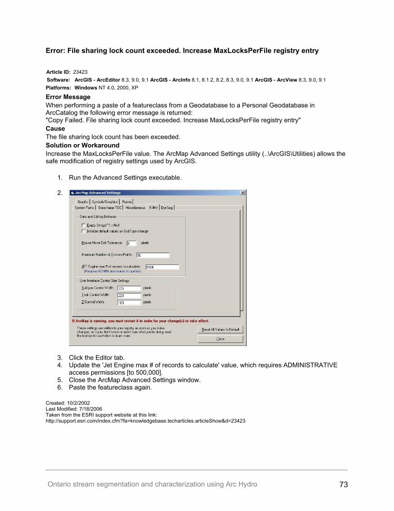
Ontario stream segmentation and characterization using Arc Hydro 73
Error: File sharing lock count exceeded. Increase MaxLocksPerFile registry entry Article ID: 23423 Software: ArcGIS - ArcEditor 8.3, 9.0, 9.1 ArcGIS - ArcInfo 8.1, 8.1.2, 8.2, 8.3, 9.0, 9.1 ArcGIS - ArcView 8.3, 9.0, 9.1Platforms: Windows NT 4.0, 2000, XP
Error Message When performing a paste of a featureclass from a Geodatabase to a Personal Geodatabase in ArcCatalog the following error message is returned: "Copy Failed. File sharing lock count exceeded. Increase MaxLocksPerFile registry entry" Cause The file sharing lock count has been exceeded. Solution or Workaround Increase the MaxLocksPerFile value. The ArcMap Advanced Settings utility (..\ArcGIS\Utilities) allows the safe modification of registry settings used by ArcGIS.
1. Run the Advanced Settings executable.
2.
3. Click the Editor tab. 4. Update the 'Jet Engine max # of records to calculate' value, which requires ADMINISTRATIVE
access permissions [to 500,000]. 5. Close the ArcMap Advanced Settings window. 6. Paste the featureclass again.
Created: 10/2/2002 Last Modified: 7/18/2006 Taken from the ESRI support website at this link: http://support.esri.com/index.cfm?fa=knowledgebase.techarticles.articleShow&d=23423
Ontario stream segmentation and characterization using Arc Hydro 74
Appendix 4: Classification Literature
Ontario stream segmentation and characterization using Arc Hydro 75
Aagaard, K. (1992). Ordination or typology - The search for a stable classification of running water communities. Netherlands Journal of Aquatic Ecology. 26(2-4): 441-445. Allan, J.D., L.B. Johnson. 1997a. Catchment-scale analysis of aquatic ecosystems. Freshwater Biology, 37: 107 -111. Allan, J.D., 1997b. The influence of catchement land se on stream integrity across multiple spatial scale. Freshwater Biology, 37: 149 – 161. Allan, J.D.. 2004. Landscapes and Riverscapes: The Influence of Landuse on Stream Ecosystems. Annual Review of Ecological Systems, 35: 257 – 284. Band, L.E., S.E. Brun, R.A. Fernandes, C.L. Tague, D.E. Tenenbaum. 2000. Modelling Watershedds as Spatial Object Hierarchies: Structure and Dynamics. Transactions in GIS, 4(3): 181 - 196 Benda, L., K. Andras, D. Miller, and P. Bigelow. 2004. Confluence effects in rivers: Interactions of basin scale, network geometry, and disturbance regimes, Water Resour. Res., 40, W05402, doi:10.1029/2003WR002583. Benda, L, N.L. Poff, D. Miller, T. Dunne, G. Reeves, G. Pess, and M. Pollock. 2004b. The Network Dymanics Hypothesis: How Channel Networks Structure Riverine Habitats. BioScience 54(5), pp. 413-427. Berman, C.. 2002. Assessment of Landscape Characterization and Classification Methods. Report for the USDA. Forest Service: WCI Cooperative Agreement No. PNW 99-9053-1-CA. Center for Water and Watershed Studies, University of Washington. Biggs, B.J.F., V.I. Nikora, T.H. Snelder. 2005. Linking scales of flow variability to lotic ecosystem structure and function. River Research and Applications, 21: 283 – 298. Bisson, P. A., and D. R. Montgomery. 1996. Valley segments, stream reaches, and channel units. Pages 23-52 in F. R. Hauer and G. A. Lanberti (eds.). Methods in Stream Ecology. Academic Press, San Diego, California. Bourgeron, P.S., Humphries, H.C., Barber, J.A., Turner, S.J., Jensen, M.E. and Goodman, I.A. (1999). Impact of broad- and fine-scale patterns on regional landscape characterization using AVHRR- derived land cover data. Ecosystem Health. 5(4): 234-258. Brunke, M., T. Gonser. 1997. The ecological significance of exchange processes between rivers and groundwater. Freshwater Biology, 37: 1 – 33. Burnett, C., T. Blaschke. 2003. A multi-scale segmentation/object relationship modelling methodology for landscape analysis. Ecological Modelling, 168: 233 – 249. Church, M.E. 2002. Geomorphic thresholds in riverine landscapes. Freshwater Biology 47: 541-557. Cohen, P., H. Andriamahefa, J. Wasson. 1998. Toward a regionalization of aquatic habitat: distribution of mesohabitats at the scale of a large basin. Regulated Rivers: Research and Management, 14: 391 – 404.
Ontario stream segmentation and characterization using Arc Hydro 76
Davies, N.M., R.H. Norris, M.C. Thoms. 2000. Prediction and assessment of local stream habitat features using large-scale catchment characteristics. Freshwater Biology, 45: 343 – 369. Dawson, F.H., D.D. Hornby, J. Hilton. 2002. A method for the automated extraction of environmental variables to help the classification of rivers in Britain. Aquatic Conservation: Marine and Freshwater Ecosystems, 12: 391 – 403. Detenbeck, N.E, V.J. Brady, D.L. Taylor, V.M. Snarski, S.L. Batterman. 2005. Relationship of stream flow regime in the western Lake Superior basin to watershed type characteristics. Journal of Hydrology: 309, 258-276. Devito, K. I. Creed, T. Gan, C. Mendoza, R. Petrone, U. Silins, B. Smerdon. 2005. A framework for broad-scale classification of hydrologic response units on the Boreal Plain: is topography the last thing to consider?. Hydrological Processes, 19: 1705 – 1714. Dollar, L.H., E.S.J. Dollar, J. Moolman. 2006. Development of an automated desktop procedure for defining macro-reaches for river longitudinal profiles. South African Water Resources Commission, Water SA 32(3) 395 – 402. Dovciak, A.L., J.A. Perry. 2002. In Search of Effective Scales for Stream Management: Does Agroecoregion, watershed, or Their Intersection Best Explain the Variance in Stream Macroinvertebrate Communities. Environmental Management, 30(3): 365 – 377. FitzHugh T.W., 2001. Watershed Characteristics and Aquatic Ecological Integrity: A Literature Review. The Nature Conservancy, Freshwater Initiative. Ferguson R.I., J.R. Cudden, T.B Hoey and S.P. Rice. 2006. River system discontinuities due to lateral inputs: generic styles and controls. Earth Surface Processes and Landforms. In press. Garbrecht, J.. 1991. Effects of Spatial Accumulation of Runoff on Watershed Response. Journal of Environmental Quality, 20: 31 – 35. Greathouse, E.A., C.M. Pringle, W.H. McDowell, J.G. Holmquist. 2006. Indirect upstream effects of dams: consequences of migratory consumer extirpation in Puerto Rico. Ecological Applications, 16(1): 339 – 352. Hall, M.J. and Minns, A.W. (1999). The classification of hydrologically homogeneous regions. Hydrological Sciences Journal. 44(5): 693–704. Harris, N.M., A.M. Gurnell, D.M Hannah, G.E. Petts. 2000. Classification of river regimes: context for hydroecology. Hydrological Processes, 14, 2831 – 2848. Hawkins, C.P., R.H. Norris, J. Gerritsen, R.M. Hughes, S.K. Jackson, R.K. Johnson, R.J. Stevenson. 2000. Evaluation of the use of landscape classification for the prediction of freshwater biota: synthesis and recommendations. Journal of the North American Benthological Society, 19(3): 541 – 556. Heino, J., H. Mykrä. 2006. Assessing physical surrogates for biodiversity: Do tributary and stream type classifications reflect macroinvertebrate assemblage diversity in running waters?. Biological Conservation, 129: 418 – 426.
Ontario stream segmentation and characterization using Arc Hydro 77
Higgins, J.V., .T. Bryer, M.L. Khoury, and T.W. FitzHugh. 2005. A Freshwater Classification Approach for Biodiversity Conservation Planning. Conservation Biology, 19(2), 432 – 445. Hynes, H.B.N. (1975). The stream and its valley. Verhandlungen der Internationale Vereinigung für Theoretische und Angewandte Limnologie. 19: 1-15. Imhof, J.G., J. Fitzgibbon, W.K. Annable. 1996. A hierarchical evaluation system for characterizing watershed ecosystems for fish habitat. Canadian Journal of Fisheries and Aquatic Sciences, 53(Suppl.1): 312 – 326. Jenerette, G.D., J. Lee, D.W. Waller, R.E. Carlson. 2002. Multivariate Analysis of the Ecoregion Delineation for Aquatic Systems. Environmental Management, 29(1): 67 – 75. Jensen, M.E., C.H. McNicoll, M. Prather. 1991. Application of Ecological Classification to Environmental Effects Analysis. Journal of Environmental Quality, 20: 24 – 30. Jensen, M.E., Goodman, I.A., Bourgeron, P.S., Poff, N.L. and Brewer, C.K. (2001). Effectiveness of biophysical criteria in the hierarchical classification of drainage basins. Journal of the American Water Resources Association. 37: 1155-1168 Johnson, L.B., S. H. Gage. 1997. Landscape approaches to the analysis of aquatic ecosystems. Freshwater Biology, 37, 113 – 132. Klijn, F., H.A.U. de Haas. 1994. A hierarchical approach to ecosystems and its implications for ecological land classification. Landscape Ecology 9(2): 89 – 104. Li, J. A. Herlihy, W. Gerth, P. Kaufmann, S. Gregory, S. Urquhart, D.P. Larsen. 2001. Variability in stream macroinvertebrates at multiple spatial scales. Freshwater Biology, 46: 87 – 97. Logan, P. and M. Furse. 2002. Preparing for the European Water Framework Directive – making the links between habitat and aquatic biota. Marine and Freshwater Ecosystems, 12: 425 – 437. Malard, F., K. Tockner, M. Dole-Olivier, J.V. Ward. 2002. A landscape perspective of surface-subsurface hydrological exchanges in river corridors. Freshwater Biology, 47, 621 – 640. Maxell, J.R., C.J. Edwards, M.E. Jensen, S.J. Paustian, H. Parrott, D.M. Hill. 1995. A Hierarchical Framework of Aquatic Ecological Units in North Amaerica (Nearctic Zone). United States Department of Agriculture, Forest Service, General Technical Report NC-176. Ministry of Northern Development and Mines. 2002. Surficial Geology of Southern Ontario-MRD 128 metadata HTML document. Ontario Geospatial Electronic Directory of Metadata for Geospatial Information Holdings. Moog, O., A. Schmidt-Kloiber, T. Ofenboeck, J. Gerritsen. 2004. Does the ecoregion approach support the typological demands of the EU ‘Water Framework Directive’?. Hydrobiologia, 516: 21 – 33. Montgomery R. and M. Buffington. 1993. Channel Classification, Prediction of Channel Response, and Assessment of Channel Condition. Report TFW-SI-110-93-002. Washington State Timber/Fish/Wildlife Agreement.
Ontario stream segmentation and characterization using Arc Hydro 78
Mykrä, H., J. Heino, T. Muotka. 2004. Variability of Lotic Macroinvertebrate Assemblages and Stream Habit Characteristics Across Hierarchical Landscape Classifications. Environmental Management, 34(2): 341 – 352. Norris, R.H. and M.C. Thoms. 1999. What is river health?. Freshwater Biology, 412: 197 – 209. Omernik, J.M. and Griffith, G.E. (1991). Ecological regions versus hydrologic units: frameworks for managing water quality. Journal of Soil and Water Conservation. 46(5): 334-340. Omnerik, J.M., R.G. Bailey. 1997. Distinguishing between watersheds and ecoregions. Journal of the American Water Resources Association, 33(5): 935 - 949. Omnerik, J.M.. 2003. The misuse of hydrologic unit maps for extrapolation, reporting, and ecosystem management. Journal of the American Water Resources Association, 39(3): 563 – 573. OMNR. 1994. Natural Channel Systems: An Approach to Management and Design. Ontario Ministry of Natural Resources. Ontario Geological Survey. 2004. Quaternary Geology of Ontario Seamless Coverage-Data Set 14 metadata text document. Ontario Geospatial Electronic Directory of Metadata for Geospatial Information Holdings. Palmer, M.A. and N.L. Poff. 1997. Heterogeneity in streams: the influence of environmental heterogeneity on patterns and processes in streams. Journal of the North American Benthological Society 16(1): 169-173. Poff, N.L..1996. A hydrogeography of unregulated streams in the United States and an examination of scale-dependence in some hydrological descriptors. Freshwater Biology, 36: 71 – 91. Poff, N. L. 1997. Landscape filters and species traits: Towards mechanistic understanding and prediction in stream ecology. Journal of the North American Benthological Society 16: 391-409. Poole, G.C.. 2002. Fluvial landscape ecology: addressing uniqueness within the river discontinuum. Freshwater Biology, 47: 641 – 660. Power, M.E., R.J. Stout, C.E. Cushing, P.P. Harper, F.R. Hauer, W.J. Matthews, P.B. Moyle, B. Statzner, I.R. Wais De Badgen. 1988. Biotic and abiotic controls in river and stream communities. Journal of the North American Benthological Society 7(4): 456-479. Pringle, C.M. 1997. Exploring how disturbance is transmitted upstream: going against the flow. Journal of the North American Benthological Society, 16(2): 425 – 438. Raven, P.J., P.J. Boon, F.H. Dawson and A.J.D. Ferguson. 1998. Towards an integrated approach to classifying and evaluating rivers in the UK. Aquatic Conservation: Marine and Freshwater Ecosystems, 8: 383 – 393.
Ontario stream segmentation and characterization using Arc Hydro 79
Rice, S.P., M.T. Greenwood, C.B. Joyce. 2001. Tributaries, sediment sources, and the longitudinal organization of macroinvertebrate fauna along river systems. Canadaian Journal of Fisheries and Aquatic Sciences, 58: 824 – 840. Richards, K. ed..1987. River Channels: Environment and Process. The Institute of British Geographers, Special Publication Series. Chapter 6, pp. 295 – 320. ISBN 0-631-14577-X. Richards, C., Johnson, L.B., and Host, G.E. 1996. Landscape-scale influences on stream habitats and biota. Canadian Journal of Fisheries and Aquatic Science 53(Suppl. 1): 295-311. Richards, C., R.J. Haro, L.B. Johnson, G.E. Host. 1997. Catchment and reach-scale properties as indicators of macroinvertebrate species traits. Freshwater Biology, 37, 219 – 230. Richardson, J.S.. 2000. Life Beyond Salmon Streams: Community of Headwaters and Their Role in Drainage Networks. British Columbia Ministry of Environment, Lands and Parks, and Forest Sciences. University of British Columbia. Richter, B.D., J.V. Baumgartner, D.P. Braun, J. Powell. 1998. A Spatial Assessment of Hydrologic Alterations within a River Network. Regulated Rivers: Research and Management, 14: 329 – 340. Robertson , D.M., D.A. Saad. 2003. Environmenatl Water-Quality Zones for Streams: A Regional Classification Scheme. Environmental Management, 31(5): 581 – 02. Rosgen, D.L. 1994. A classification of natural rivers. Catena, 22, 169 – 199. Sandin, L., R.K. Johnson. 2004. Local, landscape and regional factors structuring benthic macroinvertebrate assemblages in Swedish streams. Landscape Ecology, 19: 501 – 514. Schaefer, J.F., J.R. Kerfoot. 2004. Fish Assemblage Dynamics in an Adventitious Stream: A Landscape Perspective. American Midland Naturalist, 151: 134 – 145. Sclosser, I.J., L.W. Kallemeyn. 2000, Spatial Variation in Fish Assemblages across a beaver-influenced successional landscape. Ecology, 81(5): 1371 – 1382. Shreve, R. L. 1966. Statistical law of stream numbers. Journal of Geology 74:17–37. Sivapalan, M.. 2003a. Process complexity at hillslope scale, process simplicity at the watershed scale: is there a connection?. Hydrological Processes, 17: 1037 – 1041. Sivapalan, M., G. Bloeschl, L. Zhang, R. Vertessy. 2003b. Downward approach to hydrological prediction. Hydrological Processes, 17: 2101 – 2111. Smith, T.A., C.E. Kraft. 2005. Stream Fish Assemblages in Relation to Landscape Position and Local Habitat Variables. Transactions of the American Fisheries Society, 134: 430 – 440. Snelder, T., M. Weatherhead, R. O’Brien, U. Shankar, B. Biggs, P. Mosely. 1999. Further development and application of a GIS based river environment classification system. NIWA Client Report: CHC99/41; Project No.: NRX905. National Institute of Water & Atmospheric Research.
Ontario stream segmentation and characterization using Arc Hydro 80
Snelder, T.H., F. Cattaneo, A.M. Suren, B.J.F. Biggs. 2004. Is the River Environment Classification an improved landscape-scale classification of rivers?. Journal of the North American Benthological Society, 23(3): 580 – 598. Snelder, T.H., B.J.F. Biggs, R.A. Woods. 2005. Improved Eco-Hydrological Classification of Rivers. Rivers Research and Applications, 21: 609 – 628. Stoddard, J.L. 2005. Use of Ecological Regions in Aquatic Assessments of Ecological Conditions. Environmental Management, 34 (Suppl. 1): S61 – S70. Strahler, A.N. 1957. Quantitative Analysis of Watershed Geomorphology. Transactions, American Geophysical Union 38: 913-920. Thomson, J.R., M.P. Taylor, G.J. Brierley. 2004. Are River styles ecologically meaningful? A test of the ecological significance of a geomorphic river character scheme. Aquatic Conservation: Marine and Freshwater Ecosystems, 14: 25 – 48. Tockner, K., J.V. Ward, P.J. Edwards, J. Kollmann. 2002. Riverine Landscapes and Introduction. Freshwater Biology, 47, 497 – 500. Townsend, C. R. 1996. Concepts in river ecology: pattern and process in the catchment hierarchy. Archiv Für Hydrobiologie Supplement 113: 3-21. Turak, E., L.K. Flack, R.H. Norris, J. Simpson, N. Waddell. 1999. Assessment of river condition at a large spatial scale using predictive models. Freshwater Biology, 41: 238 – 298. Urban, D. L., R. V. O'Neill, and H. H. Shugart. 1987. Landscape ecology: a hierarchical perspective can help scientists understand spatial patterns. BioScience 37: 119-27. Vannote, R.L., G.W. Minshall, K.W. Cummins, J.R. Sedell, and C.E. Cushing. 1980. The river continuum concept. Canadian Journal of Fisheries and Aquatic Science 37: 130-137. Ward, J.V., K. Tockner, D.B. Arscott, C. Claret. 2000a. Riverine landscape diversity. Freshwater Biology, 47, 517 – 539. Ward, J.V., F. Malard, K. Tackner. 2002b. Landscape ecology: a framework for integrating patterns and process in river corridors. Landscape Ecology ,17 (Suppl. 1), 35 - 45. Wardrop, D.H., J.A. Bishop, M. Easterling, K. Hychka, W. Myers, G.P. Patil, C. Taille. 2005. Use of landscape and land use parameters for classification and characterization of watersheds in the mid-Atlantic across five physiographic provinces. Environmental and Ecological Statistics, 12: 209 – 223. Warry, N.D., M. Hanau. 1993. The use of terrestrial ecoregions as a regional-scale screen for selecting representative reference sites for water quality monitoring. Environmental Management. 17(2): 267-276.
Ontario stream segmentation and characterization using Arc Hydro 81
Wasson, J., A. Chandesris, H. Pella, L. Blanc. 2002. Typology and reference conditions for surface water bodies in France – the hydro-ecoregion approach. Symposium for Typological and ecological classification of lakes and rivers at the Finnish Environmental Institute. Whiting, P.J. and J.B. Bradley. 1993. A process-based classification system for headwater streams. Earth Surface Processes and Landforms 18: 603-612. Whittier, T.R., R.M. Hughes, D.P. Larson. 1988. Correspondence between ecoregions and spatial patterns in stream ecosystems in Oregon. Canadian Journal of Fisheries and Aquatic Sciences, 45: 1264 – 1278. Wiens, J.A. 2002. Riverine landscapes: taking landscape ecology into the water. Freshwater Biology, 47, 501 – 515. Wimmer, R., A. Chovanec, O. Moog, M.H. Fink, D. Gruber. 2000. Abiotic Stream Classification as a Basis for a Surveillance Monitoring Network in Austria in Accordance with the EU Water Framework Directive. Acta hydrochimica et hydrobiologica, 28(4): 177 - 184. Winter T.C..2001. The Concept of Hydrologic Landscapes. Journal of the American Water Resources Association, 37(2): 335 – 349. Wolock, D.M., Winter, T.C. and McMahon, G. (2004). Delineation and evaluation of hydrologic-landscape regions in the United States using geographic information system tools and multivariate statistical analyses. Environmental Management. 24(1): S71-S88. Wright, K.K. and J.L. Li. 2002. From continua to patches: examining stream community structure over large environmental gradients. Canadian Journal of Fisheries and Aquatic Science 59: 1404-1417. WRIP.2006. Factsheet No. EFDIR1: Provincial Enhanced Flow Direction Grid, Version 2.0.0. Ontario Ministry of Natural Resources – Water Resources and Information Program. Zhou, Y., S. Narumalani, W.J. Waltman, S.W. Waltman, M.A. Palecki. 2003. A GIS-based Spatial Pattern Analysis Model for Eco-region Mapping and Characterization. International Journal of Geographical Information Science, 17(5): 445 – 462.
Ontario stream segmentation and characterization using Arc Hydro 82
References FitzHugh T.W., 2005. GIS Tools for Stream and Lake Classification and Watershed Analysis: A Tool Primer. The Nature Conservancy, Freshwater Initiative. Frissell, C.A., W.J. Liss, C.E. Warren, M.D. Hurley. 1986. A Hierarchical Framework for Stream Habitat Classification: Viewing Streams in a Watershed Context. Environmental Management, 10(2): 199 – 214. Lotspeich, F.B. (1980). Watersheds as the basic ecosystem: this conceptual framework provides a basis for a natural classification system. Water Resources Bulletin. 16(4): 581-586. Seelbach P.W., M.J. Wiley, J.C. Kotanchik and M.E. Baker. 1997. A Landscape-Based Ecological Classification System For River Valley Segments in Lower Michigan (MI-VSEC Version 1.0). Fisheries Division Research Report No.2036 Michigan Department of Natural Resources. Snelder, T.H., B.J.F. Biggs. 2002. Multiscale River Environment Classification for Water Resources Management. Journal of the American Water Resources Association, 38(5): 1225 – 1239. Snelder, T., B. Biggs, and M. Weatherhead, 2004. New Zealand River Environment Classification User Guide. National Institute of Water & Atmospheric Research, New Zealand Ministry for the Environment. Snelder, T.H., K.F.D. Hughey. 2005. The Use of an Ecological Classification to Improve Water Resource Planning in New Zealand. Environmental Management, 35(5): 741 – 756. Stanfield L., R. Kuyvenhoven. 2006. Protocol for Applications used in the Aquatic Landscapes Inventory Software Application for Delineating, Characterizing and Classifying Valley Segments within the Great Lakes Basin. Ontario Ministry of Natural Resources.
Related Documents