Online fault tolerant task scheduling for real-time ...

HAL Id: tel-03016351https://hal.archives-ouvertes.fr/tel-03016351v2

Submitted on 6 Jan 2021

HAL is a multi-disciplinary open accessarchive for the deposit and dissemination of sci-entific research documents, whether they are pub-lished or not. The documents may come fromteaching and research institutions in France orabroad, or from public or private research centers.

L’archive ouverte pluridisciplinaire HAL, estdestinée au dépôt et à la diffusion de documentsscientifiques de niveau recherche, publiés ou non,émanant des établissements d’enseignement et derecherche français ou étrangers, des laboratoirespublics ou privés.

Online fault tolerant task scheduling for real-timemultiprocessor embedded systems

Petr Dobiáš

To cite this version:Petr Dobiáš. Online fault tolerant task scheduling for real-time multiprocessor embedded systems.Embedded Systems. Université Rennes 1, 2020. English. NNT : 2020REN1S024. tel-03016351v2

THÈSE DE DOCTORAT DE

ÉCOLE DOCTORALE NO 601Mathématiques et Sciences et Technologiesde l’Information et de la CommunicationSpécialité : Informatique

Par

Petr DOBIÁŠContribution à l’ordonnancement dynamique, tolérant auxfautes, de tâches pour les systèmes embarqués temps-réelmultiprocesseurs

Thèse présentée et soutenue à Lannion, le 2 octobre 2020Unité de recherche : IRISA

Rapporteurs avant soutenance :

Alberto BOSIO Professeur des Universités, Ecole Centrale de Lyon, FranceArnaud VIRAZEL Maître de Conférences, Université de Montpellier, France

Composition du Jury :

Président : Bertrand GRANADO Professeur des Universités, Sorbonne Université, FranceExaminateurs : Alberto BOSIO Professeur des Universités, Ecole Centrale de Lyon, France

Maryline CHETTO Professeur des Universités, Université de Nantes, FranceDaniel CHILLET Professeur des Universités, Université de Rennes 1, FranceOliver SINNEN Associate Professor, University of Auckland, Nouvelle ZélandeArnaud VIRAZEL Maître de Conférences, Université de Montpellier, France

Dir. de thèse : Emmanuel CASSEAU Professeur des Universités, Université de Rennes 1, FranceInvité(s) :

Prénom Nom Fonction et établissement d’exercice

RÉSUMÉ

La thèse se focalise sur le placement et l’ordonnancement dynamique des tâches sur les systèmesembarqués multiprocesseurs pour améliorer leur fiabilité tout en tenant compte des contraintes telles quele temps réel ou l’énergie. Les performances du système sont principalement évaluées par le nombre detâches rejetées, la complexité de l’algorithme et donc sa durée d’exécution et la résilience estimée eninjectant les fautes. Les contributions de la recherche sont dans les deux domaines suivants : l’approched’ordonnancement dite de « primary/backup » et la fiabilité des petits satellites appelés CubeSats.

Description de l’approche de « primary/backup »

L’approche de « primary et backup » (approche PB) considère que chaque tâche a deux copiesidentiques pour rendre le système tolérant aux fautes [61]. Ces copies sont placées sur deux processeursdifférents entre le temps d’arrivée de la tâche et sa date limite d’exécution. La première copie nomméecopie de « primary » est placée le plus tôt possible tandis que la deuxième copie appelée copie de « backup» est positionnée le plus tard possible. Pour améliorer l’ordonnancement, les copies de « backup » peuventêtre chevauchées entre elles ou désallouées si les exécutions de leurs copies de « primary » respectivessont correctes. D’autres heuristiques pour l’approche PB ont été déjà présentées [61, 103, 144, 155]. Lesfautes sont détectées par un mécanisme de détection qui signale leur occurrence.

Contributions à l’approche de « primary/backup »

Le but est de proposer des heuristiques subtiles pour réduire la durée d’exécution (mesurée à l’aidedu nombre de comparaisons) de l’algorithme d’ordonnancement tout en évitant la détérioration desperformances du système (évaluées par exemple par le taux de réjection, i.e. le nombre de tâches rejetéespar rapport au nombre total de tâches). Les contributions à l’approche PB sont les suivantes :

— l’évaluation de la surcharge de cette approche ;— la proposition d’une nouvelle stratégie d’allocation des processeurs qu’on nomme la « recherche

jusqu’à la première solution trouvée – créneau après créneau » (FFSS SbS) et qu’on compare avecd’autres stratégies déjà existantes ;

— la proposition de trois nouvelles heuristiques : (i) la méthode de limitation du nombre de compa-raisons, (ii) la méthode de limitation des fenêtres d’ordonnancement délimitant le temps pendantlequel une copie peut être placée et (iii) la méthode de plusieurs essais d’ordonnancement ;

— l’évaluation des performances de l’algorithme, en particulier en termes de nombre de comparaisonspar tâche et de taux de réjection, y compris avec l’injection des fautes ;

— la formulation mathématique du problème et la comparaison des résultats avec la solution optimaledélivrée par le solveur CPLEX ;

— l’adaptation des algorithmes proposés ci-dessus pour des tâches indépendantes afin de placer destâches dépendantes.

Analyses des résultats de l’approche de « primary/backup »

Les analyses des résultats pour les tâches indépendantes ont permis de conclure les points suivants.Le taux de réjection du système autorisant le chevauchement des copies de « backup » est réduit par

rapport au système sans aucune technique particulière (par exemple de 14% pour un système avec 14processeurs). En cas de la désallocation des copies de « backup », il est réduit encore davantage (par

iii

exemple de 75% pour un système avec 14 processeurs). De plus, les résultats montrent que les techniquesde chevauchement et de désallocation des copies de « backup » fonctionnent bien ensemble.

Le surcoût de l’approche PB qui place deux copies de la même tâche (même si la copie de « backup »peut être désallouée) a été également évalué. Quand le nombre de processeurs augmente, le nombre decomparaisons par tâche pour trouver une place pour ses copies augmente également et la différence dunombre de comparaisons entre les systèmes sans et avec approche PB devient plus importante. Néanmoins,comme il y a plus de comparaisons effectuées, la probabilité de placer une tâche augmente et donc le tauxde réjection du système tolérant aux fautes diminue et se rapproche de celui du système non-tolérant.

Ensuite, on compare les trois stratégies d’allocation des processeurs : la « recherche exhaustive » (ES),la « recherche jusqu’à la première solution trouvée – processeur après processeur » (FFSS PbP) et la« recherche jusqu’à la première solution trouvée – créneau après créneau » (FFSS SbS). L’ES a le tauxde réjection le plus bas parmi toutes les stratégies mais ses nombres moyen et maximal de comparaisonspar tâche sont au contraire les plus élevés. La méthode FFSS SbS est un bon compromis. Par exemple, letaux de réjection de FFSS SbS est de 12% plus élevé que celui d’ES pour un système avec 14 processeurset son nombre maximal de comparaisons par tâche est considérablement inférieur par rapport à celui deFFSS PbP (29% pour un système avec 14 processeurs) et à celui d’ES (41% pour un système avec 14processeurs). De plus, en comparant l’algorithme basé sur FFSS SbS à la solution optimale obtenue parun solveur CPLEX, on trouve qu’il est 2-compétitive.

Puis, deux techniques pour parcourir les processeurs sont étudiées : la « recherche basée sur lescréneaux disponibles » (FSST) et la « recherche basée sur les débuts et les fins des copies déjà placées »(BSST). La méthode BSST + ES et la méthode FSST + ES ont des nombres similaires de tâches rejetéeset BSST a besoin plus que deux fois plus de comparaisons que la FSST. Ainsi, BSST n’est pas unetechnique à choisir en termes de durée d’exécution de l’algorithme.

Après les analyses des stratégies d’allocation des processeurs et des techniques pour parcourir lesprocesseurs, on s‘intéresse aux performances des heuristiques qu’on propose.

La méthode de limitation du nombre de comparaisons montre que la définition du seuil permet deréduire le nombre maximal des comparaisons. Par exemple, si ce seuil pour les copies de « primary »est fixé à P/2 comparaisons (où P est le nombre de processeurs) et celui pour les copies de « backup »est égal à 5 comparaisons, les nombres maximal et moyen des comparaisons par tâche respectivementdiminuent de 62% et 34% tandis que le taux de réjection augmente seulement de 1,5% en comparant avecl’approche PB sans cette méthode.

La méthode de limitation des fenêtres d’ordonnancement est aussi efficace pour réduire le nombre decomparaisons sans aggraver les performances du système. Un compromis raisonnable entre le nombre decomparaisons et le taux de réjection est obtenu pour la fraction de la fenêtre de tâche égale à 0,5 ou 0,6.

La troisième heuristique proposée, plusieurs essais d’ordonnancement, vise à abaisser le taux de ré-jection des tâches. Les résultats montrent qu’il est inutile de réaliser plus que deux essais car, quand lenombre d’essais augmente, le taux de réjection ne diminue que marginalement et le nombre de comparai-sons par tâche augmente assez vite. Un bon compromis entre ces deux métriques est obtenu pour deuxessais ayant lieu à 33% de la fenêtre de tâche. Dans ce cas-là, le taux de réjection décroît de 6,2%.

En comparant les heuristiques et leurs combinaisons en termes de taux de réjection et du nombrede comparaisons, on trouve que les meilleurs résultats sont obtenus pour : (i) la méthode de limitationdu nombre de comparaisons utilisant deux essais à 33% de la fenêtre de tâche et (ii) la méthode delimitation du nombre de comparaisons. Dans le premier cas mentionné, le nombre de comparaisonsdiminue considérablement (valeur moyenne : 23% ; valeur maximale : 67%) et le taux de réjection estréduit de 4% par rapport à l’approche PB sans aucune technique d’amélioration.

Pour évaluer les performances en présence des fautes, l’algorithme proposé a été testé par l’injectiondes fautes. On a constaté que les injections des fautes allant jusqu’à 1 ·10−3 fautes par processeurs/ms ontun impact minimal. Comme cette valeur est supérieure à la valeur estimée dans les conditions standard (2·10−9 fautes par processeurs/ms [47]) et à celle dans les conditions rudes (1·10−5 fautes par processeurs/ms[118]), l’algorithme peut donc être implémenté dans les systèmes exposés à l’environnement hostile.

Afin de prolonger l’étude sur l’approche PB, l’algorithme proposé a été modifié pour gérer les tâches

iv

dépendantes modélisées par les graphes orientés acycliques (DAG). Les deux techniques pour parcourirles processeurs (FSST et BSST) combinées à trois stratégies d’allocation des processeurs (ES, FFSS PbPet FFSS SbS) ont été de nouveau comparées. Le nombre de comparaisons par DAG pour BSST + ES estconsidérablement plus élevé que pour les deux autres techniques (FSST + FFSS PbP et FSST + FFSSSbS) ce qui est dû au type de la recherche : exhaustive ou pas. Bien que la FFSS SbS et la FFSS PbPaient un taux de réjection similaire, la FFSS SbS nécessite plus de comparaisons. La méthode maximisantle chevauchement entre les copies de « backup » (BSST + ES maxOverload) a les meilleurs résultats entermes de taux de réjection mais au détriment de la durée d’exécution de l’algorithme, sauf pour lessystèmes ayant peu de processeurs. L’injection des fautes a montré que l’algorithme proposé fonctionnebien même avec les taux d’injection des fautes supérieurs aux valeurs réelles dans les conditions difficiles.

Description des CubeSats

Les CubeSats sont les petits satellites envoyés dans l’orbite basse de la Terre avec des missionsscientifiques. Leurs popularité augmente grâce à la standardisation qui réduit le budget et le tempsde développement [52]. Ils sont composés d’un ou plusieurs cubes d’arête de 10 cm et de poids maximalde 1, 3 kg [108]. À bord, il y a en général plusieurs systèmes électroniques systèmes, comme l’ordinateurde bord, le système de la détermination d’attitude et de contrôle ou le système lié à la mission (partiescientifique).

Les CubeSats sont exposés aux particules chargées et aux radiations qui causent des effets singuliers,par exemple « Single Event Upset » (SEU) et des effets de dose, comme « Total Ionizing Dose » (TID)[89]. Il est donc nécessaire de concevoir des CubeSats plus robustes. Les méthodes de robustification nesont pas de manière générale utilisées en raison des contraintes budgétaire, du temps de conception ou del’espace disponible [55]. Par exemple, il y a 43% de CubeSats qui ne mettent pas en œuvre la redondance,technique classique au niveau matériel [54, 90]. En raison de contraintes spatiales, il est préférable d’utiliserles méthodes logicielles, comme les watchdogs ou les techniques protégeant les données [3, 36, 38].

Contributions aux CubeSats

Pour améliorer la fiabilité des CubeSats, on propose de regrouper tous les processeurs à bord sur unemême carte ayant un seul système intégré. Même si cette modification peut paraître importante pour lesCubeSats actuels, elle a été déjà réalisée avec succès à bord d’ArduSat avec 17 processeurs [58]. Ainsi,il sera plus facile de protéger les processeurs, par exemple en utilisant un blindage contre les radiations[30], et d’augmenter les chances de bon déroulement de la mission car si un processeur est défectueux,d’autres processeurs qui ne sont pas dédiés à un système donné (comme c’est le cas dans les CubeSatsactuels) continuent à fonctionner.

Dans ce cadre-là, on a développé des algorithmes qui placent toutes les tâches (périodiques, sporadiqueset apériodiques) à bord de CubeSat, détectent des fautes et prennent des mesures pour délivrer desrésultats corrects. L’objectif est de minimiser le nombre de tâches rejetées en respectant les contraintestemporelles, énergétiques et la fiabilité. Ces algorithmes sont exécutés dynamiquement pour immédiate-ment réagir. Ils sont principalement dédiés aux CubeSats basés sur les processeurs commerciaux standardqui ne sont pas conçus pour l’utilisation dans l’espace contrairement aux processeurs durcis.

Les contributions dans le domaine des CubeSats sont les suivantes :— l’évaluation des performances de trois algorithmes d’ordonnancement proposés, dont un tenant

compte des contraintes énergétiques, en termes de taux de réjection, de nombre de recherchesd’ordonnancement effectuées et de durée d’exécution d’algorithme ;

— la formulation mathématique du problème et la comparaison des résultats avec la solution optimaledélivrée par le solveur CPLEX ;

— l’évaluation de la durée du fonctionnement du système en utilisant l’algorithme proposé prenanten compte les contraintes énergétiques ;

— l’injection des fautes et l’analyse de l’impact sur les performances du système ;

v

— en se basant sur les résultats obtenus, la recommandation du choix de l’algorithme à choisir.

Analyses des résultats des CubeSats

L’algorithme appelé OneOff considère toutes les tâches comme apériodiques et l’algorithme nomméOneOff&Cyclic distingue les tâches périodiques et apériodiques. Tandis que ces deux algorithmes netiennent pas compte de contraintes énergétiques, l’algorithme OneOffEnergy les considère. Tous lesalgorithmes peuvent utiliser différentes stratégies de placement pour ordonner la queue des tâches.

Les performances de OneOff et OneOff&Cyclic ont été étudiés avec trois scénarios, dont deuxproviennent de réels CubeSats. Les scénarios diffèrent par la charge du système et le rapport entre lestâches simples et doubles.

Les résultats montrent qu’il est inutile de considérer un système ayant plus de six processeurs car, siun stratégie d’ordonnancement est bien choisi, il n’y a pas de tâche rejetée. Ce choix permet donc d’éviterun système surdimensionné. De manière générale, les stratégies de placement "Earliest Deadline" pourOneOff et "Minimum Slack" pour OneOff&Cyclic minimisent bien la fonction objectif, i.e. le tauxde réjection. Elles ont également de bonnes performances en termes de durée de l’ordonnancement.

Même s’il a été trouvé que OneOff&Cyclic fonctionne moins bien que OneOff, ce dernier algo-rithme peut très bien être utilisé dans d’autres applications avec beaucoup plus de profits (par exempledans les systèmes embarqués avec les contraintes temporelles sévères) ayant moins de déclencheurs d’or-donnancement (moins de fautes, ou moins des tâches apériodiques ou moins de changements dans l’en-semble des tâches périodiques) que dans les applications étudiées.

Ainsi, les équipes construisant leurs propres CubeSats qui regroupent tous les processeurs sur uneseule carte, devraient choisir plutôt OneOff si elles hésitent entre les deux algorithmes ne prenant pasen compte les contraintes énergétiques. Néanmoins, il serait mieux d’implémenter le troisième algorithmeOneOffEnergy prenant également en compte les contraintes énergétiques.

OneOffEnergy profite de deux régimes du processeur (Run and Standby) pour réduire la consom-mation énergétique et fonctionne dans un des trois régimes (normal, safe et critical) suivant le niveaud’énergie disponible dans la batterie. Cet algorithme proposé a été évalué non seulement dans le cas desCubeSats mais aussi pour une autre application ayant des contraintes énergétiques.

Le bilan énergétique établi pour le Scénario APSS montre que la phase de communication requiertune quantité d’énergie non-négligeable en raison de la consommation importante de l’émetteur. Même sicette phase ne dure que 10 minutes ce qui est une durée plutôt courte par rapport à la période orbitaledu CubeSat étant de 95 minutes, elle peut épuiser la batterie si un algorithme tenant compte de l’aspecténergétique n’est pas implémenté. Si un tel algorithme est mis en service, il n’y a pas de risque de pénuried’énergie car l’énergie récupérée est suffisante pour couvrir toutes les dépenses énergétiques.

Pour évaluer davantage les performances de OneOffEnergy, les simulations pour une autre applicationayant des contraintes énergétiques ont été réalisées et les résultats entre OneOffEnergy et d’autresalgorithmes plus simples ont été comparés.

L’évaluation de l’utilisation du mode Standby montre des économies en énergie non-négligeables. Eneffet, elles contribuent à la durée de fonctionnement plus longue dans les régimes normal et safe ce quiréduit la réjection automatique des tâches de priorité faible. Même si le système ne fonctionnant qu’enrégime normal a un taux de réjection inférieur par rapport au système implémentant OneOffEnergy(par exemple de 19% pour le système composé de six processeurs), la capacité de la batterie ne permet pasle fonctionnement continu. Au contraire, OneOffEnergy choisit le régime de fonctionnement (normal,safe ou critical) suivant le niveau d’énergie dans la batterie, exécute les tâches avec un certain niveau depriorité pour optimiser la consommation énergétique et évite une pénurie d’énergie. Ainsi, l’algorithmeproposé présente un compromis raisonnable entre le fonctionnement du système, tel que le nombre detâches exécutées et leurs priorités, et les contraintes énergétiques.

Finalement, les simulations avec l’injection des fautes ont été réalisées. Les résultats montrent que lestrois algorithmes proposés (OneOff, OneOff&Cyclic et OneOffEnergy) fonctionnent bien mêmeen environnement hostile.

vi

ACKNOWLEDGEMENT

The author is first and foremost grateful to Dr. Emmanuel Casseau for support, frequent encourage-ment and numerous fruitful discussions we had during the development of this work.

I also owe an enormous debt of gratitude to Dr. Oliver Sinnen for his assistance, support and op-portunity to spend several months at the Parallel and Reconfigurable Computing Lab (PARC) at theUniversity of Auckland, New Zealand. Our discussions were always stimulating and greatly contributedto progress in my PhD thesis.

I am also very grateful to the research CAIRN team at the laboratory of IRISA and the research teamat the Parallel and Reconfigurable Computing Lab in Auckland, New Zealand for their support.

Last but not least, I would like to express many thanks to CubeSat teams, such as Phoenix (ArizonaState University, USA), RANGE (Georgia Institute of Technology, USA) or PW-Sat2 (Warsaw Universityof Technology, Poland) for sharing their data and discussions we had. In particular, I also wish to recognizethe members of Auckland Programme for Space Systems (APSS) for initiating me into the CubeSatproject.

vii

CONTENTS

Introduction 1

1 Preliminaries 51.1 Algorithm and System Classifications . . . . . . . . . . . . . . . . . . . . . . . . . . . . . . 51.2 Fault, Error and Failure . . . . . . . . . . . . . . . . . . . . . . . . . . . . . . . . . . . . . 71.3 Fault Models and Rates . . . . . . . . . . . . . . . . . . . . . . . . . . . . . . . . . . . . . 8

1.3.1 Processor Failure Rate . . . . . . . . . . . . . . . . . . . . . . . . . . . . . . . . . . 81.3.2 Two State Discrete Markov Model of the Gilbert-Elliott Type . . . . . . . . . . . . 91.3.3 Mathematical Distributions . . . . . . . . . . . . . . . . . . . . . . . . . . . . . . . 111.3.4 Comparison of Fault/Failures Rates in Space and No-Space Applications . . . . . . 13

1.4 Redundancy . . . . . . . . . . . . . . . . . . . . . . . . . . . . . . . . . . . . . . . . . . . . 171.5 Dynamic Voltage and Frequency Scaling . . . . . . . . . . . . . . . . . . . . . . . . . . . . 191.6 Summary . . . . . . . . . . . . . . . . . . . . . . . . . . . . . . . . . . . . . . . . . . . . . 20

2 Primary/Backup Approach: Related Work 212.1 Advent . . . . . . . . . . . . . . . . . . . . . . . . . . . . . . . . . . . . . . . . . . . . . . . 212.2 Baseline Algorithm with Backup Overloading and Backup Deallocation . . . . . . . . . . 212.3 Processor Allocation Policy . . . . . . . . . . . . . . . . . . . . . . . . . . . . . . . . . . . 23

2.3.1 Random Search . . . . . . . . . . . . . . . . . . . . . . . . . . . . . . . . . . . . . . 232.3.2 Exhaustive Search . . . . . . . . . . . . . . . . . . . . . . . . . . . . . . . . . . . . 232.3.3 Sequential Search . . . . . . . . . . . . . . . . . . . . . . . . . . . . . . . . . . . . . 242.3.4 Load-based Search . . . . . . . . . . . . . . . . . . . . . . . . . . . . . . . . . . . . 25

2.4 Improvements . . . . . . . . . . . . . . . . . . . . . . . . . . . . . . . . . . . . . . . . . . . 252.4.1 Primary Slack . . . . . . . . . . . . . . . . . . . . . . . . . . . . . . . . . . . . . . . 252.4.2 Decision Deadline . . . . . . . . . . . . . . . . . . . . . . . . . . . . . . . . . . . . 262.4.3 Active Approach . . . . . . . . . . . . . . . . . . . . . . . . . . . . . . . . . . . . . 272.4.4 Replication Cost and Boundary Schedules . . . . . . . . . . . . . . . . . . . . . . . 282.4.5 Primary-Backup Overloading . . . . . . . . . . . . . . . . . . . . . . . . . . . . . . 29

2.5 Fault Tolerance of the Primary/Backup Approach . . . . . . . . . . . . . . . . . . . . . . 302.6 Dependent Tasks . . . . . . . . . . . . . . . . . . . . . . . . . . . . . . . . . . . . . . . . . 32

2.6.1 Experimental Framework . . . . . . . . . . . . . . . . . . . . . . . . . . . . . . . . 342.6.2 Generation of DAGs . . . . . . . . . . . . . . . . . . . . . . . . . . . . . . . . . . . 35

2.7 Application of Primary/Backup Approach . . . . . . . . . . . . . . . . . . . . . . . . . . . 382.7.1 Dynamic Voltage and Frequency Scaling . . . . . . . . . . . . . . . . . . . . . . . . 382.7.2 Evolutionary Algorithms . . . . . . . . . . . . . . . . . . . . . . . . . . . . . . . . . 402.7.3 Virtualised Clouds . . . . . . . . . . . . . . . . . . . . . . . . . . . . . . . . . . . . 432.7.4 Satellites . . . . . . . . . . . . . . . . . . . . . . . . . . . . . . . . . . . . . . . . . 44

2.8 Summary . . . . . . . . . . . . . . . . . . . . . . . . . . . . . . . . . . . . . . . . . . . . . 45

3 Primary/Backup Approach: Our Analysis 473.1 Independent Tasks . . . . . . . . . . . . . . . . . . . . . . . . . . . . . . . . . . . . . . . . 47

3.1.1 Assumptions and Scheduling Model . . . . . . . . . . . . . . . . . . . . . . . . . . 473.1.2 Experimental Framework . . . . . . . . . . . . . . . . . . . . . . . . . . . . . . . . 573.1.3 Results . . . . . . . . . . . . . . . . . . . . . . . . . . . . . . . . . . . . . . . . . . 59

3.2 Dependent Tasks . . . . . . . . . . . . . . . . . . . . . . . . . . . . . . . . . . . . . . . . . 75

ix

CONTENTS

3.2.1 Assumptions and Scheduling Model . . . . . . . . . . . . . . . . . . . . . . . . . . 763.2.2 Scheduling Methods . . . . . . . . . . . . . . . . . . . . . . . . . . . . . . . . . . . 763.2.3 Methods to Deal with DAGs . . . . . . . . . . . . . . . . . . . . . . . . . . . . . . 773.2.4 Experimental Framework . . . . . . . . . . . . . . . . . . . . . . . . . . . . . . . . 813.2.5 Results . . . . . . . . . . . . . . . . . . . . . . . . . . . . . . . . . . . . . . . . . . 82

3.3 Summary . . . . . . . . . . . . . . . . . . . . . . . . . . . . . . . . . . . . . . . . . . . . . 95

4 CubeSats and Space Environment 974.1 Satellites . . . . . . . . . . . . . . . . . . . . . . . . . . . . . . . . . . . . . . . . . . . . . . 974.2 CubeSats . . . . . . . . . . . . . . . . . . . . . . . . . . . . . . . . . . . . . . . . . . . . . 98

4.2.1 Mission . . . . . . . . . . . . . . . . . . . . . . . . . . . . . . . . . . . . . . . . . . 994.2.2 Systems . . . . . . . . . . . . . . . . . . . . . . . . . . . . . . . . . . . . . . . . . . 1024.2.3 General Tasks . . . . . . . . . . . . . . . . . . . . . . . . . . . . . . . . . . . . . . . 104

4.3 Space Environment . . . . . . . . . . . . . . . . . . . . . . . . . . . . . . . . . . . . . . . . 1064.4 Fault Tolerance of CubeSats . . . . . . . . . . . . . . . . . . . . . . . . . . . . . . . . . . . 1084.5 Fault Detection, Isolation and Recovery Aboard CubeSats . . . . . . . . . . . . . . . . . . 1094.6 Summary . . . . . . . . . . . . . . . . . . . . . . . . . . . . . . . . . . . . . . . . . . . . . 111

5 Online Fault Tolerant Scheduling Algorithms for CubeSats 1135.1 Our Idea . . . . . . . . . . . . . . . . . . . . . . . . . . . . . . . . . . . . . . . . . . . . . . 1135.2 No-Energy-Aware Algorithms . . . . . . . . . . . . . . . . . . . . . . . . . . . . . . . . . . 113

5.2.1 System, Fault and Task Models . . . . . . . . . . . . . . . . . . . . . . . . . . . . . 1135.2.2 Presentation of Algorithms . . . . . . . . . . . . . . . . . . . . . . . . . . . . . . . 1155.2.3 Experimental Framework . . . . . . . . . . . . . . . . . . . . . . . . . . . . . . . . 1205.2.4 Results . . . . . . . . . . . . . . . . . . . . . . . . . . . . . . . . . . . . . . . . . . 122

5.3 Energy-Aware Algorithm . . . . . . . . . . . . . . . . . . . . . . . . . . . . . . . . . . . . . 1335.3.1 System, Fault and Task Models . . . . . . . . . . . . . . . . . . . . . . . . . . . . . 1335.3.2 Presentation of Algorithm . . . . . . . . . . . . . . . . . . . . . . . . . . . . . . . . 1345.3.3 Energy and Power Formulae . . . . . . . . . . . . . . . . . . . . . . . . . . . . . . 1345.3.4 Experimental Framework for CubeSats . . . . . . . . . . . . . . . . . . . . . . . . . 1375.3.5 Results for CubeSats . . . . . . . . . . . . . . . . . . . . . . . . . . . . . . . . . . . 1395.3.6 Experimental Framework for Another Application . . . . . . . . . . . . . . . . . . 1445.3.7 Results for Another Application . . . . . . . . . . . . . . . . . . . . . . . . . . . . 1465.3.8 Summary . . . . . . . . . . . . . . . . . . . . . . . . . . . . . . . . . . . . . . . . . 151

6 Conclusions 155

A Adaptation of the Boundary Schedule Search Technique 159A.1 Primary Copies . . . . . . . . . . . . . . . . . . . . . . . . . . . . . . . . . . . . . . . . . . 159A.2 Backup Copies . . . . . . . . . . . . . . . . . . . . . . . . . . . . . . . . . . . . . . . . . . 160

A.2.1 No BC Overloading . . . . . . . . . . . . . . . . . . . . . . . . . . . . . . . . . . . 160A.2.2 BC Overloading Authorised . . . . . . . . . . . . . . . . . . . . . . . . . . . . . . . 160

B DAGGEN Parameters 163

C Constraint Programming Parameters 165

D Box Plot 167

Publications 169

Bibliography 181

x

LIST OF FIGURES

1.1 Causal chain of failure . . . . . . . . . . . . . . . . . . . . . . . . . . . . . . . . . . . . . . 71.2 Bathtub curve . . . . . . . . . . . . . . . . . . . . . . . . . . . . . . . . . . . . . . . . . . . 81.3 Two state Gilbert-Elliott model for burst errors . . . . . . . . . . . . . . . . . . . . . . . . 101.4 Origin of system failures . . . . . . . . . . . . . . . . . . . . . . . . . . . . . . . . . . . . . 161.5 Principle of redundancy . . . . . . . . . . . . . . . . . . . . . . . . . . . . . . . . . . . . . 19

2.1 Example of scheduling one task . . . . . . . . . . . . . . . . . . . . . . . . . . . . . . . . . 222.2 Example of backup overloading . . . . . . . . . . . . . . . . . . . . . . . . . . . . . . . . . 222.3 Example of the primary slack . . . . . . . . . . . . . . . . . . . . . . . . . . . . . . . . . . 262.4 Example of the decision deadline . . . . . . . . . . . . . . . . . . . . . . . . . . . . . . . . 272.5 Principle of the active primary/backup approach . . . . . . . . . . . . . . . . . . . . . . . 272.6 Example of boundary and non-boundary "schedules" . . . . . . . . . . . . . . . . . . . . . 282.7 Example of the primary-backup overloading . . . . . . . . . . . . . . . . . . . . . . . . . . 312.8 Difference between ∆f and ∆F . . . . . . . . . . . . . . . . . . . . . . . . . . . . . . . . . 312.9 An example of the general directed acyclic graph (DAG) . . . . . . . . . . . . . . . . . . . 322.10 Difference between strong and weak primary copies . . . . . . . . . . . . . . . . . . . . . . 332.11 Example of DAG generation using DAGGEN . . . . . . . . . . . . . . . . . . . . . . . . . 362.12 Example of DAG generation using the TGFF . . . . . . . . . . . . . . . . . . . . . . . . . 372.13 Schedules generated by two algorithms using different allocation policies . . . . . . . . . . 392.14 Structure of the solution vector . . . . . . . . . . . . . . . . . . . . . . . . . . . . . . . . . 412.15 Structure of the population . . . . . . . . . . . . . . . . . . . . . . . . . . . . . . . . . . . 412.16 Example of available opportunity . . . . . . . . . . . . . . . . . . . . . . . . . . . . . . . . 45

3.1 Principle of the primary/backup approach . . . . . . . . . . . . . . . . . . . . . . . . . . . 483.2 Principle of the First Found Solution Search (FFSS) . . . . . . . . . . . . . . . . . . . . . 503.3 Examples of free slots . . . . . . . . . . . . . . . . . . . . . . . . . . . . . . . . . . . . . . 513.4 Different possibilities to place a new task copy when scheduling using the BSST . . . . . . 513.5 Example of boundary and non-boundary slots . . . . . . . . . . . . . . . . . . . . . . . . . 523.6 Mean and maximum numbers of comparisons per task . . . . . . . . . . . . . . . . . . . . 533.7 Mean numbers of comparisons per task as a function of the number of processors . . . . . 533.8 Maximum number of comparisons per task as a function of the number of processors . . . 533.9 Theoretical limitation on the maximum number of comparisons per task . . . . . . . . . . 543.10 Number of occurrences of task start or end time as a function of the position in the tw . . 553.11 Primary/backup approach with restricted scheduling windows (f = 1/3) . . . . . . . . . . 553.12 Example of theoretical maximum run-time . . . . . . . . . . . . . . . . . . . . . . . . . . . 563.13 Three scheduling attempts at ω = 25% . . . . . . . . . . . . . . . . . . . . . . . . . . . . 563.14 System metrics for PB approach with and without BC overloading . . . . . . . . . . . . . 603.15 System metrics for PB approach with BC deallocation with and without BC overloading . 623.16 Statistical distribution of tasks with regard to their computation times . . . . . . . . . . . 633.17 Evaluation of the active PB approach . . . . . . . . . . . . . . . . . . . . . . . . . . . . . 643.18 System metrics for active PB approach . . . . . . . . . . . . . . . . . . . . . . . . . . . . . 653.19 Three processor allocation policies and evaluation of system overheads . . . . . . . . . . . 653.20 Scheduling search techniques (PB approach + BC deallocation) . . . . . . . . . . . . . . . 67

xi

LIST OF FIGURES

3.21 Scheduling search techniques (PB approach + BC deallocation + BC overloading) . . . . 673.22 Method of limitation on the number of comparisons . . . . . . . . . . . . . . . . . . . . . 683.23 Method of restricted scheduling windows . . . . . . . . . . . . . . . . . . . . . . . . . . . . 693.24 Restricted scheduling windows as a function of the fractions of task window for PC and BC 703.25 Method of several scheduling attempts . . . . . . . . . . . . . . . . . . . . . . . . . . . . . 713.26 Improvements to a 14-processor system . . . . . . . . . . . . . . . . . . . . . . . . . . . . 713.27 Comparison of different methods for the PB approach with BC deallocation . . . . . . . . 723.28 Improvements to a 14-processor system (best parameters) . . . . . . . . . . . . . . . . . . 733.29 Improvements to a 14-processor system (best parameters; FFSS SbS compared to ES) . . 743.30 Total number of faults against the number of processors . . . . . . . . . . . . . . . . . . . 743.31 System metrics at different fault injection rates . . . . . . . . . . . . . . . . . . . . . . . . 753.32 Example of a general directed acyclic graph (DAG) . . . . . . . . . . . . . . . . . . . . . . 763.33 Example of a DAG . . . . . . . . . . . . . . . . . . . . . . . . . . . . . . . . . . . . . . . . 803.34 Example of generated DAGs . . . . . . . . . . . . . . . . . . . . . . . . . . . . . . . . . . . 813.35 Rejection rate as a function of the number of processors and number of tasks (T P L = 0.5) 833.36 Rejection rate as a function of the number of processors and number of tasks (T P L = 1.0) 833.37 Processor load as a function of the number of processors and number of tasks . . . . . . . 843.38 Ratio of computation times as a function of the number of processors and number of tasks 853.39 Mean number of compar. per DAG as a function of the numbers of processors and tasks . 853.40 Rejection rate as a function of the number of processors and size of task window . . . . . 863.41 Ratio of computation times as a function of the number of processors and size of tw . . . 873.42 Mean number of compar. per DAG as a function of the number of processors and size of tw 873.43 Rejection rate as a function of the number of processors (T P L = 0.5) . . . . . . . . . . . 883.44 Rejection rate as a function of the number of processors (T P L = 1.0) . . . . . . . . . . . 883.45 Ratio of computation times as a function of the number of processors . . . . . . . . . . . 883.46 Mean number of comparisons per DAG as a function of the number of processors . . . . . 893.47 Rejection rate as a function of the number of tasks . . . . . . . . . . . . . . . . . . . . . . 893.48 Mean number of comparisons per DAG as a function of the number of tasks . . . . . . . . 903.49 Rejection rate as a function of the size of the task window . . . . . . . . . . . . . . . . . . 903.50 Mean number of comparisons per DAG as a function of the size of the task window . . . . 903.51 Total number of faults (1 · 10−5 fault/ms) against the number of processors . . . . . . . . 913.52 Total number of faults (4 · 10−4 fault/ms) against the number of processors . . . . . . . . 923.53 Total number of faults (1 · 10−3 fault/ms) against the number of processors . . . . . . . . 923.54 Total number of faults (1 · 10−2 fault/ms) against the number of processors . . . . . . . . 923.55 Rejection rate at different fault injection rates (10 tasks in one DAG) . . . . . . . . . . . 933.56 Rejection rate at different fault injection rates (100 tasks in one DAG) . . . . . . . . . . . 933.57 System throughout at different fault injection rates (10 tasks in one DAG) . . . . . . . . . 943.58 System throughout at different fault injection rates (100 tasks in one DAG) . . . . . . . . 943.59 Processor load at different fault injection rates (10 tasks in one DAG) . . . . . . . . . . . 943.60 Mean number of compar. per DAG at different fault injection rates (10 tasks in one DAG) 95

4.1 Comparison of satellites . . . . . . . . . . . . . . . . . . . . . . . . . . . . . . . . . . . . . 984.2 Phoenix (3U) CubeSat . . . . . . . . . . . . . . . . . . . . . . . . . . . . . . . . . . . . . . 994.3 Number of launched nanosatellites per year . . . . . . . . . . . . . . . . . . . . . . . . . . 1004.4 Cumulative sum of launched nanosatellites . . . . . . . . . . . . . . . . . . . . . . . . . . . 1004.5 Number of launched satellites by institution . . . . . . . . . . . . . . . . . . . . . . . . . . 1014.6 Number of launched satellites by countries . . . . . . . . . . . . . . . . . . . . . . . . . . . 1014.7 Communication phase and no-communication phase . . . . . . . . . . . . . . . . . . . . . 1044.8 Space environment . . . . . . . . . . . . . . . . . . . . . . . . . . . . . . . . . . . . . . . . 1064.9 Number of launched nanosatellites and their status . . . . . . . . . . . . . . . . . . . . . . 108

xii

LIST OF FIGURES

4.10 Use of redundancy aboard CubeSats . . . . . . . . . . . . . . . . . . . . . . . . . . . . . . 109

5.1 Model of aperiodic task ti . . . . . . . . . . . . . . . . . . . . . . . . . . . . . . . . . . . . 1145.2 Model of periodic task τi . . . . . . . . . . . . . . . . . . . . . . . . . . . . . . . . . . . . . 1145.3 Principle of scheduling task copies . . . . . . . . . . . . . . . . . . . . . . . . . . . . . . . 1155.4 Principle of the algorithm search for a free slot on processors . . . . . . . . . . . . . . . . 1165.5 Principle of the method to reduce the number of scheduling searches . . . . . . . . . . . . 1185.6 Theoretical processor load of CubeSat scenarios . . . . . . . . . . . . . . . . . . . . . . . . 1235.7 Proportion of simple and double tasks . . . . . . . . . . . . . . . . . . . . . . . . . . . . . 1235.8 Rejection rate (OneOff; communication phase) . . . . . . . . . . . . . . . . . . . . . . . 1245.9 Rejection rate (OneOff; no-communication phase) . . . . . . . . . . . . . . . . . . . . . . 1245.10 Number of victories for "All techniques" method (OneOff; Scenario APSS) . . . . . . . . 1255.11 Rejection rate (OneOff&Cyclic; communication phase) . . . . . . . . . . . . . . . . . . 1255.12 Rejection rate (OneOff&Cyclic; no-communication phase) . . . . . . . . . . . . . . . . 1255.13 Proportion of simple and double tasks against the rejection rate . . . . . . . . . . . . . . . 1265.14 Number of scheduling searches . . . . . . . . . . . . . . . . . . . . . . . . . . . . . . . . . 1275.15 Number of scheduling searches (OneOff; Scenario APSS) . . . . . . . . . . . . . . . . . . 1285.16 Rejection rate (OneOff; Scenario APSS) . . . . . . . . . . . . . . . . . . . . . . . . . . . 1285.17 Scheduling time (Scenario APSS; no-communication phase) . . . . . . . . . . . . . . . . . 1295.18 Scheduling time (Scenario RANGE; no-communication phase) . . . . . . . . . . . . . . . . 1295.19 Mean value of task queue length with standard deviations (OneOff) . . . . . . . . . . . 1305.20 Scheduling time (Scenario APSS-modified; no-communication phase) . . . . . . . . . . . . 1315.21 Total number of faults against the number of processors . . . . . . . . . . . . . . . . . . . 1315.22 System metrics at different fault injection rates (OneOff; communication phase) . . . . . 1325.23 System metrics at different fault injection rates (OneOff; no-communication phase) . . . 1325.24 Theoretical processor load of CubeSat scenario to evaluate OneOffEnergy . . . . . . . 1405.25 Rejection rate for three system modes . . . . . . . . . . . . . . . . . . . . . . . . . . . . . 1405.26 Useful and idle energy consumptions during two hyperperiods (communication phase) . . 1415.27 CubeSat power consumption in three system modes . . . . . . . . . . . . . . . . . . . . . 1415.28 Energy supplied and energy needed aboard the CubeSat . . . . . . . . . . . . . . . . . . . 1425.29 Energy in the battery against time (communication phase in the eclipse) . . . . . . . . . . 1435.30 System and processor loads against time (communication phase in the eclipse) . . . . . . 1435.31 Energy in the battery against time (communication in the daylight) . . . . . . . . . . . . 1435.32 System and processor loads against time (communication phase in the daylight) . . . . . . 1445.33 Rejection rate as a function of the number of processors and the initial battery energy . . 1445.34 Theoretical processor load of CubeSat scenario to evaluate OneOffEnergy . . . . . . . 1465.35 Energy in the battery against time . . . . . . . . . . . . . . . . . . . . . . . . . . . . . . . 1475.36 System and processor loads against time . . . . . . . . . . . . . . . . . . . . . . . . . . . . 1475.37 Energy in the battery against time to assess system operation . . . . . . . . . . . . . . . . 1485.38 Overall time spent in different system modes . . . . . . . . . . . . . . . . . . . . . . . . . 1495.39 System and processor loads against time to assess system operation . . . . . . . . . . . . . 1495.40 System metrics as a function of the number of processors . . . . . . . . . . . . . . . . . . 1505.41 Total number of faults against the number of processors . . . . . . . . . . . . . . . . . . . 1515.42 System metrics at different fault injection rates (OneOffEnergy) . . . . . . . . . . . . . 151

A.1 Example of the search for a PC slot using the BSST + FFSS PbP . . . . . . . . . . . . . 159A.2 Example of search for a slot for BC . . . . . . . . . . . . . . . . . . . . . . . . . . . . . . . 160A.3 Different cases of BC scheduling with BC overloading . . . . . . . . . . . . . . . . . . . . 161

xiii

LIST OF FIGURES

B.1 Levels of DAG . . . . . . . . . . . . . . . . . . . . . . . . . . . . . . . . . . . . . . . . . . 163B.2 Example of DAG parameter "fat" . . . . . . . . . . . . . . . . . . . . . . . . . . . . . . . . 163B.3 Example of DAG parameter "density" . . . . . . . . . . . . . . . . . . . . . . . . . . . . . 164B.4 Example of DAG parameter "regularity" . . . . . . . . . . . . . . . . . . . . . . . . . . . . 164B.5 Example of DAG parameter "jump" . . . . . . . . . . . . . . . . . . . . . . . . . . . . . . 164

D.1 Example of a box plot . . . . . . . . . . . . . . . . . . . . . . . . . . . . . . . . . . . . . . 167

xiv

LIST OF TABLES

1.1 Commonly used values of λi and d . . . . . . . . . . . . . . . . . . . . . . . . . . . . . . . 91.2 Fault or failure rates in no-space applications . . . . . . . . . . . . . . . . . . . . . . . . . 141.3 Fault or failure rates in space applications . . . . . . . . . . . . . . . . . . . . . . . . . . . 141.4 Failure rate of high-performance computers . . . . . . . . . . . . . . . . . . . . . . . . . . 151.5 Failure rates at the International Space Station . . . . . . . . . . . . . . . . . . . . . . . . 171.6 Fault injection into UPSat . . . . . . . . . . . . . . . . . . . . . . . . . . . . . . . . . . . . 18

2.1 Constraints on mapping of primary copies of dependent tasks . . . . . . . . . . . . . . . . 342.2 Simulation parameters for dependent tasks modelled by DAGs . . . . . . . . . . . . . . . 352.3 DAG parameters . . . . . . . . . . . . . . . . . . . . . . . . . . . . . . . . . . . . . . . . . 36

3.1 Notations and definitions . . . . . . . . . . . . . . . . . . . . . . . . . . . . . . . . . . . . 483.2 Simulation parameters . . . . . . . . . . . . . . . . . . . . . . . . . . . . . . . . . . . . . . 583.3 Task copy position . . . . . . . . . . . . . . . . . . . . . . . . . . . . . . . . . . . . . . . . 773.4 Example of tasks with their computation times and assigned start times and deadlines . . 803.5 Parameters to generate DAGs . . . . . . . . . . . . . . . . . . . . . . . . . . . . . . . . . . 813.6 Simulation parameters . . . . . . . . . . . . . . . . . . . . . . . . . . . . . . . . . . . . . . 823.7 Comparison of our results with the ones already published for the 16-processor system . . 91

4.1 Comparison of communication parameters for three orbits . . . . . . . . . . . . . . . . . . 1034.2 Parameters of several CubeSats . . . . . . . . . . . . . . . . . . . . . . . . . . . . . . . . . 1054.3 Component characteristics at low Earth orbit (altitude < 2 000 km) . . . . . . . . . . . . 107

5.1 Notations and definitions . . . . . . . . . . . . . . . . . . . . . . . . . . . . . . . . . . . . 1145.2 Set of tasks for Scenario APSS . . . . . . . . . . . . . . . . . . . . . . . . . . . . . . . . . 1205.3 Set of tasks for Scenario RANGE . . . . . . . . . . . . . . . . . . . . . . . . . . . . . . . . 1215.4 Set of tasks for Scenario APSS-modified . . . . . . . . . . . . . . . . . . . . . . . . . . . . 1215.5 Number of task copies for three scenarios . . . . . . . . . . . . . . . . . . . . . . . . . . . 1215.6 System operating modes . . . . . . . . . . . . . . . . . . . . . . . . . . . . . . . . . . . . . 1335.7 Several characteristics of STM32F103 processor . . . . . . . . . . . . . . . . . . . . . . . . 1335.8 Number of processors in Standby mode . . . . . . . . . . . . . . . . . . . . . . . . . . . . 1345.9 Set of tasks for Scenario APSS taking into account energy constraints . . . . . . . . . . . 1375.10 Simulation parameters related to time . . . . . . . . . . . . . . . . . . . . . . . . . . . . . 1385.11 Simulation parameters related to power and energy . . . . . . . . . . . . . . . . . . . . . . 1385.12 Other power consumption aboard a CubeSat taken into account . . . . . . . . . . . . . . 1385.13 Simulation parameters . . . . . . . . . . . . . . . . . . . . . . . . . . . . . . . . . . . . . . 1455.14 Simulation parameters related to time . . . . . . . . . . . . . . . . . . . . . . . . . . . . . 1455.15 Simulation parameters related to power and energy . . . . . . . . . . . . . . . . . . . . . . 145

C.1 Several constraint programming setting parameters . . . . . . . . . . . . . . . . . . . . . . 165C.2 Example of the influence of parameter settings . . . . . . . . . . . . . . . . . . . . . . . . 166

xv

LIST OF ALGORITHMS

1 Algorithm using the exhaustive search . . . . . . . . . . . . . . . . . . . . . . . . . . . . . 242 Algorithm using the sequential search . . . . . . . . . . . . . . . . . . . . . . . . . . . . . 243 Algorithm using the load-based search . . . . . . . . . . . . . . . . . . . . . . . . . . . . . 254 Implementation of the primary-backup overloading . . . . . . . . . . . . . . . . . . . . . . 305 Determination of start times and deadlines of tasks in DAG . . . . . . . . . . . . . . . . . 346 Primary/backup scheduling . . . . . . . . . . . . . . . . . . . . . . . . . . . . . . . . . . . 507 Algorithm using the method of several scheduling attempts . . . . . . . . . . . . . . . . . 578 Main steps to find the optimal solution of a scheduling problem in CPLEX optimiser . . . 589 Generation of directed acyclic graphs . . . . . . . . . . . . . . . . . . . . . . . . . . . . . . 7710 Main steps to schedule dependent tasks . . . . . . . . . . . . . . . . . . . . . . . . . . . . 7811 Forward method to determine a deadline . . . . . . . . . . . . . . . . . . . . . . . . . . . . 7812 Determination of start times and deadlines of tasks in DAG in our experimental framework 7913 Online algorithm scheduling all tasks as aperiodic tasks (OneOff) . . . . . . . . . . . . . 11714 Online algorithm scheduling all tasks as periodic or aperiodic tasks (OneOff&Cyclic) . 11915 Online energy-aware algorithm scheduling all tasks as aperiodic tasks (OneOffEnergy) 135

xvii

LIST OF ACRONYMS

ADCS Attitude Determination and Control System.ALAP As Late As Possible.ASAP As Soon As Possible.

BC Backup Copy.BSST Boundary Schedule Search Technique.

CDHS Command and Data Handling System.COM COMmunication system.COTS Commercial Off-The-Shelf.CP+NCP Communication Phase and No-Communication Phase.CPU Central Processing Unit.

DAG Directed Acyclic Graph.DOA Dead On Arrival.DOD Depth Of Discharge.DVFS Dynamic Voltage and Frequency Scaling.

EPS Electrical Power System.ES Exhaustive Search.

FFSS SbS First Found Solution Search: Slot by Slot.FFSS PbP First Found Solution Search: Processor by Processor.FSST Free Slot Search Technique.

HPC High-Performance Computing.HT Hyperperiod.

ISS International Space Station.

LANL Los Alamos National Laboratory.LEO Low Earth Orbit.LET Linear Energy Transfer.

MIPS Million Instructions Per Second.MTBF Mean Time Between Faults.MTTF Mean Time To Faults.MTTR Mean Time To Repair.

NASA National Aeronautics and Space Administration.NCP No-Communication Phase.

OBC On-Board Computer.

PB Primary/Backup.PC Primary Copy.

RX Receiver.

xix

List of Acronyms

SEB Single Event Burnout.SEE Single Event Effect.SEFI Single Event Functional Interrupt.SEGR Single Event Gate Rupture.SEL Single Event Latch-up.SEMBE Single Event Multiple Bit Error.SET Single Event Transient.SEU Single Event Upset.SLOC Source Lines Of Codes.

TGFF Task Graph For Free.TID Total Ionising Dose.TMR Triple Modular Redundancy.TPL Targeted Processor Load.TTNF Time To Next Fault.TX Transmitter.

xx

INTRODUCTION

Every system component is liable to fail and it will cease to correctly run sooner or later. As aconsequence, the system can exhibit a malfunction. There are applications where a system failure canhave catastrophic consequences such as advanced driver-assistance systems, air traffic control or medicalequipment. In order to deal with this problem, systems should be fault tolerant. It means that such asystem is more robust, can tolerate several faults and properly works even if faults occur.

In general, requirements on multiprocessor embedded systems for higher performance and lower energyconsumption are increasing so that they might meet demands of more and more complex computations.Moreover, the transistors are scaling down and their operating voltage is getting lower, which goes handin glove with higher susceptibility to system failure.

Since systems are more vulnerable to faults, the reliability becomes the main concern [105]. Thereare various methods to provide systems with fault tolerance and the choice of the design depends ona particular application [49, 72, 85]. For multiprocessor embedded systems, one of promising methodsmakes use of reconfigurable computing and/or redundancy in space or in time. In addition, multiprocessorsystems are less vulnerable than a standalone processor because, in case of a processor failure, otherprocessors remain operational.

The focus of this PhD thesis is dual. We first deal with the primary/backup approach for failureelimination techniques and then with some aspects of scheduling algorithm design of small satellitescalled CubeSats. In both cases, we are concerned with multiprocessor embedded systems with aim toimprove their reliability.

The primary/backup approach is a method of fault tolerant scheduling on multiprocessor embeddedsystems making use of two task copies: the primary and backup ones [61]. It is a commonly used techniquefor designing fault tolerant systems owing to its easy application and minimal system overheads. Severaladditional enhancements [61, 103, 144, 155] to this approach have been already presented but few studiesdealing with overall comparisons have been published. Moreover, the resiliency of the primary/backupapproach has been discussed in only few studies and with several restrictive assumptions.

CubeSats are small satellites consisting of several processors and subject to strict space and weightconstraints [108]. They operate in the harsh space environment, where they are exposed to chargedparticles and radiation [89]. Since the CubeSat fault tolerance is not always considered, e.g., due tobudget or time constraints, their vulnerability to faults can jeopardise the mission [54, 90]. Our aim isto improve the CubeSat reliability. The proposed solution again makes use of an online fault tolerantscheduling on multiprocessor embedded systems. It is mainly meant for CubeSats based on commercial-off-the-shelf processors, which are not necessarily designed to be used in space applications and thereforemore vulnerable to faults than radiation hardened processors.

Scope of Research

The scope of the PhD thesis is also dual: the first one is related to the primary/backup approach andthe second one is concerned with scheduling algorithms for CubeSats to improve their reliability.

Regarding the primary/backup approach, our main objective is to choose enhancing method(s),which significantly reduce(s) the algorithm run-time without worsening system performances when onlinescheduling tasks on embedded systems. The scope of research meant for the scheduling of independenttasks is as follows:

— Evaluation of the overheads of the primary/backup approach;

1

Introduction

— Introduction of a new processor allocation policy (called first found solution search: slot by slot)and its comparison with already existing processor allocation policies;

— Introduction and analysis of three new enhancing techniques based on the primary/backup ap-proach: (i) the method of restricted scheduling windows within which the primary and backupcopies can be scheduled, (ii) the method of limitation on the number of comparisons, accountingfor the algorithm run-time, when scheduling a task on a system, and (iii) the method of severalscheduling attempts;

— Discussion of the trade-off between the algorithm run-time (measured by the number of compar-isons to find a free slot) and system performances (assessed by the rejection rate, i.e. the ratio ofrejected tasks to all arriving tasks);

— Mathematical programming formulation of the scheduling problem and comparison of our resultswith the optimal solution delivered by CPLEX solver;

— Assessment of the fault tolerance of the primary/backup approach when scheduling independenttasks.

The scope designed for dependent tasks is as reads:— Adaptations of the scheduling algorithms of independent tasks for dependent ones;— Evaluation of the scheduling algorithms in terms of their performances and compare them with

the already known ones for the dependent tasks;— The fault tolerance analysis for scheduling dependent tasks.

Regarding CubeSats, our aim is to minimise the number of rejected tasks subject to real-time, relia-bility and energy constraints. The scope of research related to CubeSats is as follows:

— Assessment of performances of three proposed algorithms in terms of the rejection rate (which againrepresents the ratio of rejected tasks to all arriving tasks), the number of scheduling searches andthe scheduling time for different scenarios;

— Mathematical programming formulation of the scheduling problem; whenever possible we comparethe results to the optimal solution provided by CPLEX solver;

— Evaluation of the devised energy-aware algorithm in terms of the system operation and the energyconsumption;

— Analyses of the presented algorithms regarding their treatment of faults;— Based on performances of these algorithms, the suggestion which algorithm should be used on

board of the CubeSat.

Paper Organisation

The thesis is organised as follows.

To make the reader familiar with the context of the PhD thesis, Chapter 1 presents an overviewof several topics closely related to the carried out research and gives several definitions to introducemain terms, which will be used throughout the thesis. This chapter sums up system, algorithm and taskclassifications. Then, it summarises fault models, based on either the Markov model or mathematicaldistributions, and gives some examples of fault rates for applications being executed on the Earth andalso in space. Next, we present redundancy, which is a commonly used technique to provide systems withfault tolerance. Finally, the dynamic voltage and frequency scaling is described and we discuss whetherits use is reasonable for systems aiming at maximising the reliability.

After this general context, the next two chapters focus on the primary/backup approach. While Chap-ter 2 presents the fundamentals, the related work and several applications, Chapter 3 covers our research.Its first part is devoted to independent tasks and the second one treats dependent tasks. For each type oftasks, we first introduce the task, system and fault models. Then, we describe our experimental frameworkand analyse the results. In particular, this chapter presents and compares different processor allocationpolicies and scheduling search techniques. It introduces the proposed enhancing techniques: the method

2

Introduction

of restricted scheduling windows, the one of limitation on the number of comparisons, and the one ofseveral scheduling attempts.

Chapters 4 and 5 deal with small satellites called CubeSats. Chapter 4 introduces and classifies themamong other satellites according to their weight and size. We also mention the advent and show theirprogressive popularity and their missions. Next, we describe the space environment and how CubeSatsare vulnerable to faults. Finally, we sum up the methods currently used to provide CubeSats with faulttolerance. To overcome the harsh space environment, Chapter 5 presents a solution to improve theCubeSat reliability. To analyse its performances, the system, task and fault models are defined andthe three proposed scheduling algorithms are introduced. While the first two presented algorithms do nottake energy constraints into account, the last devised algorithm is energy-aware. After the description ofthe experimental frameworks, the results in a fault-free and harsh environments are discussed.

Chapter 6 concludes the thesis by summing the main achievements and suggestions.

The thesis includes four appendices. Appendix A details how the exhaustive search of “boundaryschedule search technique” was adapted for the “first found solution search: processor by processor”,which does not carry out an exhaustive search. Appendix B lists and describes the input parameterswhen the directed acyclic graphs (DAGs) are generated using the task graph generator called DAGGEN.Appendix C presents several constraint programming parameters having influence on reproducibility ofresults and Appendix D explains the graphical representation of the box plot.

3

Chapter 1

PRELIMINARIES

This chapter presents an overview of several topics closely related to the present manuscript of thePhD thesis. First, it sums up system, algorithm and task classifications. Second, it distinguishes termsassociated with fault tolerant systems. Third, it summarises fault models and gives some examples of faultrates. Fourth, redundancy, which is one of the techniques to make system more robust against faults, isintroduced. Fifth, the use of dynamic voltage and frequency scaling is discussed.

1.1 Algorithm and System Classifications

We present several types of classifications from the viewpoints of systems, algorithms and tasks. Weremind the reader that the lists are not exhaustive and include terms, which allow us to clearly defineour research problems in this manuscript.

We start to give two definitions. We call mapping, a placing of a task onto one of the system processorstaking into account already scheduled tasks, and scheduling, a placing of a task onto one particular systemprocessor taking into account already scheduled tasks on it.

To describe a system, its main characteristics related to scheduling are generally as reads:— Uniprocessor/Multiprocessor

While a uniprocessor system has only one processor, a multiprocessor system has more than one.In general, scheduling on multiprocessor systems is a NP problem, which means that it is noteasy to find an optimal solution and the use of heuristics is necessary. In fact, a problem is saidto be NP, accounting for nondeterministic polynomial time, if it is solvable in polynomial timeby a nondeterministic Turing machine. Such a machine is able to perform parallel computationswithout communications among them [151, 152].

— Homogeneous/heterogeneous processorsIf a system is multiprocessor, it consists either of homogeneous or heterogeneous processors. Al-though systems composed of heterogeneous processors generally provide better performance be-cause a scheduling algorithm can take advantage of distinct features of processors, the schedulingcomplexity is higher when compared to systems with homogeneous processors [132].A more detailed classification formulated by Graham in [66] allows us to further characterise asystem by conventional letters:— P denotes identical parallel machines, i.e. machines having the same processing frequency.— Q stands for uniform parallel machines, which means that each machine has its own frequency.— R represents unrelated parallel machines.— O means an open shop, i.e. each job Jj consists of a set of operations O1j , . . . , O1m. The order

of these operations is not important but Oij has to be executed on machine Mj during pij timeunits.

— F denotes a flow shop. Each job Jj is a set of operations O1j , . . . , O1m and the order of theseoperations has to be respected. Oij has to be executed on machine Mj during pij time units.

— J is a job shop. Each job Jj consists of a set of operations O1j , . . . , O1m and the order of theseoperations has to be respected. Oij has to be executed on a given machine µij during pij timeunits with µi−1,j 6= µij for i = 2, . . . , m.

— Real-time aspectThree categories are distinguished from the real-time point of view based on the respect of task

5

Chapter 1 – Preliminaries

deadline [96, 117]. If hard real-time systems, such as space and aircraft applications or nuclearplant control, miss a task deadline, subsequent consequences may be catastrophic. For firm real-time systems, like online transaction processing and reservation systems, a respect of deadline isimportant because the results provided after the task deadline are not useful anymore but thereare no dire consequences. Finally, the results delivered after the task deadline by soft real-timesystem, e.g. image processing applications, are utilisable but may be less pertinent.

A scheduling algorithm, which is generally run on a scheduler, has its main attributes as follows:— Online versus Offline

An offline, also called static or design-time, algorithm knows all problem data in advance, for ex-ample number of tasks and their characteristics, such as arrival times, execution times or deadlines.When tasks arrive over time and a scheduling algorithm does not have any knowledge of any futuretasks, the algorithm is called online, also named dynamic or run-time [117, 119, 125, 132, 134].While online scheduling offers the possibility to adapt to system changes and task arrivals, it hashigher computational cost than offline scheduling.In case of online scheduling, we distinguish whether an algorithm is clairvoyant or non-clairvoyant[119]. While a clairvoyant algorithm is aware of all task attributes at the arrival time, a non-clairvoyant one notices that a new task arrives but the task characteristics are not available. Forinstance, the task execution time is known once a task was executed.

— Competitive ratioTo evaluate performances of an online algorithm a competitive analysis is carried out. An onlinealgorithm A is called c-competitive if, for all inputs, the objective function value of a schedulecomputed by A is at most a factor of c away from that of an optimal schedule [125].For example, we consider that we want to minimise an objective function of a given schedulingproblem. For any input I, let A(I) be the objective function value achieved by A on I and letOP T (I) be the value of an optional solution for I. An online algorithm A is called c-competitiveif there exists a constant b independent of the input such that, for all problem inputs I, A(I) 6

c · OP T (I) + b [125]. The competitive ratio is basically equivalent to a worst-case bound [119].— Global versus Partitioned

If an algorithm schedules tasks on a multiprocessor system, there are two possibilities how itconsiders the system [117, 132]. If it considers only one task queue and one system sharing theresources, it is called global or centralised. Otherwise, each processor (or group of processors) has itsown task queue and its own resources. In this case, we call it partitioned or distributed scheduling.

Regarding task characteristics, the ones related to our work are as follows:— Periodicity

The periodicity defines whether a task is repeated or not. While a periodic task arrives at regularintervals, an aperiodic task arrives only once. To complete this classification, we mention thatthere are also sporadic tasks having a minimal time between two arrivals. Every task can be thenfurther characterised, for example by arrival time, computation time, deadline or priority. Whena new scheduling problem is introduced in this manuscript, a precise definition of task and itsattributes are given (for more details see Sections 3.1.1 and 3.2.1 for primary/backup approachand Section 5.2.1 for CubeSats).

— Precedence constraintsBased on the existence of precedence constraints, we distinguish independent and dependent tasks.

— PreemptionA scheduling algorithm is called preemptive if it authorises to temporarily suspend running taskshaving lower priority than a new arriving task and preferentially execute this new task. Otherwise,it is called non-preemptive and it does not interrupt currently executing tasks and new tasks canstart after currently executing tasks finish their execution [117].

A scheduling problem is also defined by its optimality criteria. The most commonly used optimality

6

1.2. Fault, Error and Failure

criteria are related to time performance, for instance completion time or lateness, but other objectivefunctions become more and more frequent, such as energy consumption or reliability. Since demands onperformance increases, one objective function may not be sufficient and a multi-objective problems areformulated. To solve such a problem, one can choose from three possibilities [125]:

— Transform some objectives into constraints.— Decompose the multi-objective problem to several problems with a single objective, sort objective

functions according to the importance and treat each objective separately.— Use the Pareto curve to find an optimal solution, i.e. the one where it is not possible to decrease

the value of one objective without increasing the value of the other [119].Nowadays, systems are more and more vulnerable to faults and the reliability, i.e. the ability of a

system to perform a required function under given conditions for a given time interval, becomes themain concern. Naithani et al. [105, 106] thus emphasized the necessity to consider the reliability aspectduring scheduling. They showed that it is better to make use of reliability-aware scheduling rather thanperformance-optimised scheduling. On average, although the reliability-aware scheduling degrades per-formance by 6%, it improves the system reliability by 25.4% compared to the performance-optimisedscheduling.

In order to standardise the classification of scheduling problems, Graham et al. [66] proposed a 3-field notation α|β|γ in 1979. The parameter α refers to the processor environment, while the parameterβ represents task characteristics and the parameter γ stands for the objective function. An overview ofscheduling algorithms based on Graham classification is available at the website http://schedulingzoo.

lip6.fr/.

1.2 Fault, Error and Failure

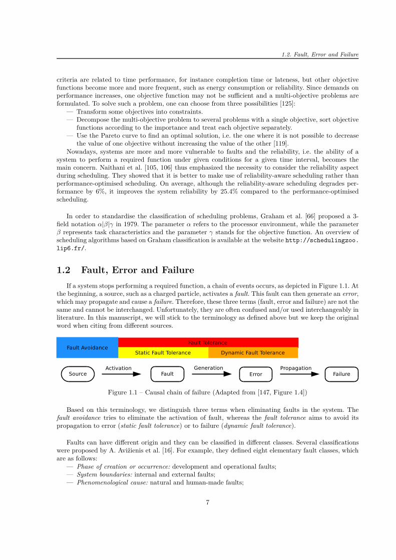
If a system stops performing a required function, a chain of events occurs, as depicted in Figure 1.1. Atthe beginning, a source, such as a charged particle, activates a fault. This fault can then generate an error,which may propagate and cause a failure. Therefore, these three terms (fault, error and failure) are not thesame and cannot be interchanged. Unfortunately, they are often confused and/or used interchangeably inliterature. In this manuscript, we will stick to the terminology as defined above but we keep the originalword when citing from different sources.

Figure 1.1 – Causal chain of failure (Adapted from [147, Figure 1.4])

Based on this terminology, we distinguish three terms when eliminating faults in the system. Thefault avoidance tries to eliminate the activation of fault, whereas the fault tolerance aims to avoid itspropagation to error (static fault tolerance) or to failure (dynamic fault tolerance).

Faults can have different origin and they can be classified in different classes. Several classificationswere proposed by A. Avižienis et al. [16]. For example, they defined eight elementary fault classes, whichare as follows:

— Phase of creation or occurrence: development and operational faults;— System boundaries: internal and external faults;— Phenomenological cause: natural and human-made faults;

7

Chapter 1 – Preliminaries

— Domain: hardware and software faults;— Objective: malicious and non-malicious faults;— Intent: deliberate and non-deliberate faults;— Capability: accidental and incompetence faults;— Persistence: permanent and transient faults.

We note that one fault can be classified in several classes. For example, a charged particle in spacecan be classified as an operational, external, natural, non-malicious and non-deliberate fault. Its furtherclassification then depends on the impact location (hardware or software) and duration (permanent ortransient).

As regards the fault detection, isolation and recovery, there are various approaches and they aremainly application dependent. A general overview was presented in the previous work of the author[43, 44]. Consequently, since the primary/backup approach is a general method and the fault detectiondepends on its application, only list of general techniques is given in Section 3.1.1. Regarding CubeSats,the context is specific and, subsequently, a more detailed presentation of fault detection and recoverytechniques is provided in Section 4.5.

1.3 Fault Models and Rates

We will introduce the processor failure rate and different possibilities how a fault injection and/oranalysis can be carried out when evaluating algorithm performances. The first possibility is to make useof a Markov model, which is a probabilistic approach to evaluate the reliability of systems with constantfailure rate. The second one is based on mathematical distributions, both discrete and continuous ones.Finally, different fault/failures rates in space and no-space applications will be compared.

1.3.1 Processor Failure Rate

Let us introduce the failure 1 rate λ, which is defined as the expected number of failures per timeunit. In general, the failure rate varies in the course of time. There are more failures at the beginning ofthe lifetime due to not yet defined problems and at its end due to ageing effects. Therefore, its temporalrepresentation depicted in Figure 1.2 resembles to a bathtub curve having three main phases: (1) infantmortality, (2) useful life and (3) wear-out.

Time t

Failu

rera

teλ

////

Infant mortalityphase

Useful lifephase

Wear-outphase

Figure 1.2 – Bathtub curve (Adapted from [85, Figure 2.1])

1. In literature, the terms failure and fault are often confused or used interchangeably. In this manuscript, while we keepthe original word when citing from different sources, we stick to the terminology as defined in Section 1.2.

8

1.3. Fault Models and Rates

In general, the failure rate λ depends on many factors, such as age, technology or environment. In[85], the authors give the following empirical formula taking into account different factors:

λ = πLπQ(C1πT πV + C2πE)

where— πL: learning factor, related to the level of technology development,— πQ: quality factor (∈ [0, 25; 20]) accounting for manufacturing process quality control,— πT : temperature factor (∈ [0, 1; 1000]),— πV : voltage stress factor for CMOS (Complementary Metal Oxide Semiconductor) depending on

the supply voltage and the temperature (∈ [1; 10]), for other devices it is equal to 1,— πE : environment shock factor (∈ [0, 4; 13]),— C1, C2: complexity factors, functions of the number of gates on the chip and the number of pins

in the package.

The failure rate can be also expressed as a function of the processor frequencies [88, 123, 148, 153].We note λi,j the failure rate of processor Pj when executing task ti at frequency fi,j. This rate can becomputed as reads

λi,j = λi · 10d(fmaxi

−fi,j)fmaxi

−fmini (1.1)

where— λi is the average failure rate of task ti when the frequency is equal to the maximum frequency of

task ti denoted as fmaxi,

— d is a constant indicating the sensitivity of failure rates to voltage and frequency scaling.Formula 1.1 is frequently used to determine the value of λ when there are no reliability data for a studiedsystem. Commonly used values for λi and d are summarised in Table 1.1.

Table 1.1 – Commonly used values of λi and d

Reference λi d

[158] 10−6 0, 2, 4, 6[41] 10−6 3

[70, 71] 10−6 4

[153] [2 · 10−4 to 6 · 10−4] 2.1, 2.3, 2.5[88] [10−3 to 10−8] 2, 3

As an example of the system vulnerability, we mention that big cores are in general more vulnerableto bit flips than small cores because they consist of more transistors [105, 106]. Nevertheless, big coresexecute faster, which reduces the exposure to faults during task execution.

Another possibility is to determine the failure rate using the probability theory [130] and exploitthe reliability data that were already measured. It means that the value of λ or other parameters arecomputed based on a distribution. In order to determine parameters for a given distribution, once dataof fault occurrences are available, they are analysed and modelled with different distributions (presentedin Section 1.3.3) to find the best fit to the measured data.

1.3.2 Two State Discrete Markov Model of the Gilbert-Elliott Type

We introduce a Markov model, which is a probabilistic approach to evaluate the reliability of systemswith constant failure rate [85].

The origin of name dates back to 1960, when E. N. Gilbert presented a Markov model of a burst-noisebinary channel [62]. He considered two states: G (abbreviation of Good) and B (abbreviation of Bad

9

Chapter 1 – Preliminaries

or Burst). In state G, transmission is error-free and, in state B, a digit is transmitted correctly withprobability h. Three years later, E. O. Elliott improved this model and estimated error rates for codeson burst-noise channels [51]. At that time, the model was employed to provide close approximation tocertain telephone circuits used for the transmission of binary data.

In 2013, M. Short and J. Proenza studied real-time computing and communication systems in a harshenvironment, i.e. when a system is exposed to random errors and random bursts of errors [131]. Theypointed out that, if the classical fault tolerant schedulability analysis is put into service, it may notcorrectly represent randomness or burst characteristics. Modern approaches could solve this issue but atthe cost of increased complexity. Consequently, the authors decided to make use of the simple two-statediscrete Markov model of the Gilbert-Elliott type to provide a reasonable fault analysis without significantincrease in complexity. This model accounts for a "Markov-Modulated Poisson Binomial" process on oneprocessor and it well represents errors, which are random and uncorrelated in nature but occur in shorttransient burst.

pGB

pBG

1 − pGB 1 − pBG

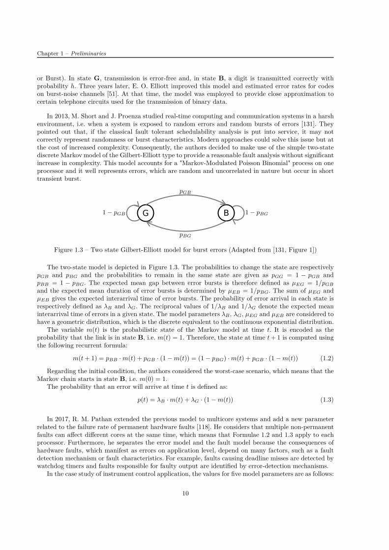
Figure 1.3 – Two state Gilbert-Elliott model for burst errors (Adapted from [131, Figure 1])

The two-state model is depicted in Figure 1.3. The probabilities to change the state are respectivelypGB and pBG and the probabilities to remain in the same state are given as pGG = 1 − pGB andpBB = 1 − pBG. The expected mean gap between error bursts is therefore defined as µEG = 1/pGB

and the expected mean duration of error bursts is determined by µEB = 1/pBG. The sum of µEG andµEB gives the expected interarrival time of error bursts. The probability of error arrival in each state isrespectively defined as λB and λG. The reciprocal values of 1/λB and 1/λG denote the expected meaninterarrival time of errors in a given state. The model parameters λB , λG, µEG and µEB are considered tohave a geometric distribution, which is the discrete equivalent to the continuous exponential distribution.

The variable m(t) is the probabilistic state of the Markov model at time t. It is encoded as theprobability that the link is in state B, i.e. m(t) = 1. Therefore, the state at time t + 1 is computed usingthe following recurrent formula:

m(t + 1) = pBB · m(t) + pGB · (1 − m(t)) = (1 − pBG) · m(t) + pGB · (1 − m(t)) (1.2)

Regarding the initial condition, the authors considered the worst-case scenario, which means that theMarkov chain starts in state B, i.e. m(0) = 1.

The probability that an error will arrive at time t is defined as:

p(t) = λB · m(t) + λG · (1 − m(t)) (1.3)

In 2017, R. M. Pathan extended the previous model to multicore systems and add a new parameterrelated to the failure rate of permanent hardware faults [118]. He considers that multiple non-permanentfaults can affect different cores at the same time, which means that Formulae 1.2 and 1.3 apply to eachprocessor. Furthermore, he separates the error model and the fault model because the consequences ofhardware faults, which manifest as errors on application level, depend on many factors, such as a faultdetection mechanism or fault characteristics. For example, faults causing deadline misses are detected bywatchdog timers and faults responsible for faulty output are identified by error-detection mechanisms.

In the case study of instrument control application, the values for five model parameters are as follows:

10

1.3. Fault Models and Rates

— Failure rate of permanent hardware faults in multicore chip: λc = 10−5/h— Failure rate of random non-permanent hardware faults in each core during a non-bursty period

(G state): λG = 10−4/h— Failure rate of random non-permanent hardware faults in each core during a burst (B state):

λB = 10−2/s— Expected duration of one non-bursty period (G state): µEG = 1/pGB = 106 ms— Expected duration of one bursty 2 period (B state): µEB = 1/pBG = 102 ms

The Markov model is also used to compute the reliability in satellites, such as in [56]. In this publi-cation, Markov models were analysed to study the reliability of on board computer (OBC) in four cases:a centralized OBC (which corresponds to the case represented in Figure 1.3), an OBC based on TMR,an OBC using task migration between two processors, and an OBC using task migration and three pro-cessors. It was shown that OBCs making use of task migration have higher reliability because when aprocessor is faulty, all tasks scheduled on it can be migrated to healthy processors. Therefore, the higherthe number of processors, the higher the reliability.

1.3.3 Mathematical Distributions

The system reliability can be also modelled using several distributions. The most common distri-butions, which are used to model fault occurrences, are presented in this section after giving severaldefinitions.

Let us consider a probability space (Ω, F ,P), where— Ω is a set of all possible outcomes,— F is a set of events and a subset of Ω,— P is a function assigning the probabilities to events [139].We define a random variable X corresponding to a processor lifetime, i.e. the time until it fails. Since

values of the lifetime are positive, X is mapped in real positive values, such as

X : Ω −→ R+

ω 7−→ X(ω)

We can then distinguish two cases: whether the random variable X is discrete or continuous.

1.3.3.1 Discrete Random Variable X

If X is a discrete random variable, then X(Ω) is a countable set, i.e. X(Ω) = N. An example of adiscrete probability distribution is the Poisson distribution with parameter λ > 0 defined as:

∀k ∈ N,P(X = k) = e−λ λk

k!(1.4)

where the value of k represents the number of faults.The Poisson distribution assumes that faults are independent and the parameter λ denotes a constant

failure rate per time unit. If this parameter is multiplied by time t (expressed in time units) to representa specific number of occurrences within a given time interval [12, 162], then the probability that k faultsoccur in time t is given as:

∀k ∈ N,P(X = k) = e−λt (λt)k

k!

and the reliability, i.e. the probability of zero failures in time t, is expressed as:

R = P(X = 0) = e−λt (λt)0

0!= e−λt (1.5)

2. Based on the related work, R. M. Pathan mentions that a burst length is 5µs [118].

11

Chapter 1 – Preliminaries

The Poisson distribution is widely used in no-space applications [5, 41, 60, 68, 79, 88, 94, 99, 102,123, 136, 143, 148, 153, 154, 156, 158, 159] because the assumption of constant failure rate is verifiedin most applications during the useful life, i.e. the second phase of the bathtub curve represented inFigure 1.2. Although this assumption may not be always valid in the harsh space environment, thePoisson distribution was also considered in space applications, for example in [32].

1.3.3.2 Continuous Random Variable X

If X is a continuous random variable, X(Ω) is in most cases an interval or a union of intervals andthe probability is defined using a density function f(t) [85, 139]. In our context, X is positive since itrepresents a processor lifetime and therefore the density function f(t) satisfies:

∀t > 0, f(t) > 0 and∫

∞

0

f(t)dt = 1

The cumulative distribution function of X , denoted by FX(t), represents the probability that theprocessor will fail at or before time t. It is defined as follows:

FX(t) = P(X 6 t) =∫ t

0

f(τ)dτ

Finally, the reliability R(t) is the probability that a processor will survive at least until time t, whichmeans that

R(t) = P(t < X) = 1 − FX(t)

After giving the previous definitions, we now express the failure rate λ(t), which is a conditionalprobability because we know that the processor correctly functioned at least until time t. It can becomputed as reads:

λ(t) =f(t)

1 − FX(t)

We note that the failure rate depends on a cumulative distribution function FX(t) and a probabilitydensity function f(t). The probability density functions, which are often considered to model faults, areas follows [85, 91, 139]:

— Weibull distribution is defined as reads:

f(t) = λβtβ−1e−λtβ

λ(t) = λβtβ−1

R(t) = e−λtβ

where λ > 0 is a scale parameter and β > 0 is a shape parameter.This distribution is appropriate to the bathtub curve, especially to model “infant mortality” and“wear-out” phases. Consequently, it can be considered as a general one to model well all cyclephases.It is considered for example in [41, 133] for no-space applications. Regarding space applications,it is convenient to model all satellite lifetime. For example, researchers studied failure data fromCubeSats and they found out that this distribution has the best fit to measured data [54, 92].

— Exponential distribution is characterised by

f(t) = λe−λt

λ(t) = λ

R(t) = e−λt (1.6)

12

1.3. Fault Models and Rates

The exponential distribution is a special case of the Weibull distribution with β = 1 and assumesa constant failure rate λ > 0, which is valid during the "useful life" phase of the bathtub curve.This distribution is commonly used due its simplicity.It can be noticed [12] that, if we consider that a processor will not fail as long as no fault occurs,Formula 1.6, accounting for the reliability of exponential distribution, equals Formula 1.5, standingfor the reliability of Poisson distribution.Due to its simplicity, this distribution is commonly used to model faults in no-space applications,for example in [9, 25, 45, 70, 71, 82, 149], and even in space applications, for instance in [56].

— Lognormal distribution is expressed as follows:

f(t) =1

xσ√

2πe

−12

(

ln(x)−µ

σ

)2

where µ and σ denote the mean and standard deviation, respectively.This distribution takes into account variations of failure rates throughout the processor lifetime[156] and it was used for example in [146] to model faults at the International Space Station.

In literature, when the reliability of task ti is computed, the value of t generally represents theexecution time of task ti. For example, when considering the Poisson or exponential distributions, whichhave the same expression of the reliability (Formulae 1.5 and 1.6), the reliability of task ti is

R = e−λeti

where eti is the execution time of task ti, for example in [41, 70, 71, 88, 99, 123, 143, 148, 153, 158].

1.3.4 Comparison of Fault/Failures Rates in Space and No-Space Applica-tions

The fault/failure rate also depends on the number of processors in the system. Intuitively, if there aremore processors in the system, faults arrive more frequently.

In [72], the authors considered that a system consists of N identical processors and that each processoris characterised by its reliability measured by means of Mean Time Between Faults (MTBF) denoted byµind. They proved that the overall system reliability µ is divided by the number of processors:

µ =µind

N(1.7)

which means that if we for example double the number of components, the system resiliency (in terms ofthe MTBF) is divided by two.

To complete the definitions, the MTBF is related to the Mean Time To Failure (MTTF) and theMean Time To Repair (MTTR). If we consider that a processor repair is always perfect and the repairedsystem performs as the original system, these three times are related as follows [49]:

MT BF = MT T F + MT T R (1.8)

In order to draw a comparison between fault/failures occurrences on the Earth and in space, fault/fail-ure rates for no-space and space applications are respectively summed up in Tables 1.2 and 1.3. The dataare classified according to fault/failure duration, i.e. whether only permanent or transient faults/failuresor both together are considered. The rates are given per hour but in some cases they are expressed pertime unit because the time unit was not specified in several papers. Last but not least, for each rate, wenote a considered component (node, processor, system, ...).

The rates of permanent faults/failures are lower when compared to transient ones. In addition, ratesare generally higher in space than on the ground because space is a harsh environment due to chargedparticles and radiation.

In the next three sections, we focus on three applications (high-performance computers, the Interna-tional Space Station and CubeSats) to further analyse the fault/failure rates.

13

Chapter 1 – Preliminaries

Table 1.2 – Fault or failure rates in no-space applications

Permanent faults or failures

Reference Fault or failure rate Application

[159] Node: 1 · 10−7 failure/hour Heterogeneous clusters

[122] Processor: 1 · 10−6 to 7.5 · 10−6 failure/hour Heterogeneous systems

Transient faults or failures

Reference Fault or failure rate Application

[41, 158] Processor: 10−6 fault/(unit of time) Real-time embedded systems

[153] Processor: 2 · 10−4 to 6 · 10−4 fault/(unit of time) Heterogeneous embedded systems

[79] Node: 1.5 · 10−3 to 2.5 · 10−3 failure/hour Parallel system with 256 nodes

[158]100 megabit chip: 10−5 to ∼ 10−3 fault/hour

Whole system: 10−3 to ∼ 101 fault/hourReal-time embedded systems

Transient and permanent faults or failures

Reference Fault or failure rate Application

[99] System: 1 · 10−5 to 5 · 10−5 failure/(unit of time) Heterogeneous computing systems

Type of faults or failures not mentioned

Reference Fault or failure rate Application

[68] Processor: 5 · 10−6 to 15 · 10−6 failure/hour Heterogeneous computing systems

[143] Processor: 1 · 10−4 to 7.5 · 10−4 failure/hour Heterogeneous computing systems

[9] Processor: 1 · 10−4 to 1 · 10−3 failure/hour Homogeneous clusters

Table 1.3 – Fault or failure rates in space applications

Permanent faults or failures

Reference Fault or failure rate Application

[118] Processor: 10−5 fault/hour Safety-critical multicore systems

Transient faults or failures

Reference Fault or failure rate Application

[17, 32] System: 10−2 to 102 fault/hourDifferent satellite and aircraft

applications

[30] 512 kbytes SRAM block: 4 fault/hour OBC of small satellite

[118]Processor: 10−4 fault/hour (during no-bursty period)

Whole chip: 101 fault/hour (during bursty period)Safety-critical multicore systems

Transient and permanent faults or failures

Reference Fault or failure rate Application

[56] Processor: 1 · 10−3 failure/hour Satellite on-board computer (OBC)

1.3.4.1 Failures in High-Performance Computers

The High-Performance Computers (HPC) are computing systems consisting of several processors.Such systems are for example used for large-scale long-running 3D scientific simulations, such as plasmaflow analysis [130]. The fault tolerance of HPC is frequently implemented as checkpointing [130]. Thismethod consists in periodic saving of data during the execution. If a fault occurs in the course of taskexecution, it is restarted from the last checkpoint or from scratch if no checkpoint exists.

In this section, we consider the following HPC systems: Los Alamos National Laboratory (LANL),

14

1.3. Fault Models and Rates

Blue Waters, Tsubame, Mercury and one anonymous supercomputing site. The performances of thesesystems were already analysed in papers [15, 20, 130], which we will briefly summarise.

L. Bautista-Gomez et al. [20] evaluated occurrences of transient failures in Blue Waters, Tsubame,Mercury and LANL. They found out that there are periods with up to three times higher failure densitywhen compared to other periods and they proposed dynamic checkpointing to detect such periods andsave time.

If we assume that the MTTR is negligible when compared with MTTF and that the failure rate λ isconstant, which is not accurate since the failure rate varies over system lifetime [130] (see Sections 1.3.1and 1.3.3 for more details), we can approximately compute the number of failures per hour based on theirdata related to MTBF using Formula 1.8 and the following relation for failure rate:

λ =1

MT T F

Knowing the system characteristics, we then evaluate failure rates for studied systems and their coresthanks to Formula 1.7. The results are summarised in Table 1.4.

Table 1.4 – Failure rate of high-performance computers (Based on data from [20, Table 1])

System MTBF (h) Failures per h # cores MTBF (h)/core Failures per h per core

Blue Waters 11.2 8.93 · 10−2 25 000 28 000 3.57 · 10−5

Tsubame 10.4 9.62 · 10−2 74 358 715 324 1.40 · 10−6

Mercury 16.0 6.25 · 10−2 891 14 256 7.01 · 10−5

LANL 23.0 4.35 · 10−2 24 101 327 888 3.05 · 10−6

It is also interesting to analyse origin of failures of four systems. As Figures 1.4 show, the majority offailures occurs in hardware and failures in software have the second largest percentage. The authors of[130], who analysed the failure data of LANL, stated that the most common hardware failure is due tocentral processing unit (CPU) (about 40%).

To give an example of failures, the authors of [20] found out that the most frequent failures of Mercuryare as follows:

— errors in memory that were not correctable by Error Correction Code (ECC),— processor cache errors,— hardware-reported error in a device on the SCSI (Small Computer System Interface) bus,— NFS (Network File System)-related error indicating unavailability of the network file system for a

machine,— PBS (Portable Batch System) daemon failure to communicate.

B. Schroeder and G. A. Gibson studied failure data from two HPC sites [130]. The first data setwas collected over 9 years at LANL containing data from 22 high-performance computing systems (4750machines and 24101 processors). The second data set was at an anonymous supercomputing site com-prising 20 nodes and 10 240 processors. Their aim was to study statistical properties of the available dataconsisting of 23 000 failures.

First, they fitted their data using three probability distributions: the Poisson one, the normal oneand the lognormal one. They estimated the maximum likelihood to parametrise the distributions andevaluated their fits. They found out that the Poisson distribution, which is often considered in faultanalysis, does not represent well the data and that the normal and lognormal distributions fit better.

Moreover, when analysing the time between failures, the exponential distribution does not fit well butthe gamma or Weibull distributions with decreasing hazard rate (Weibull shape parameter of 0.7-0.8)achieve better results. The hazard rate defines how the time since the last failure influences the expectedtime until the next failure. The studied data, which have a decreasing hazard rate, show that the longerthe time since last failure, the longer expected time until next failure.

15

Chapter 1 – Preliminaries

Hardware47.1%

Software33.7%

Network11.8%

Environmental

3.3%

Other

4.0%

(a) Blue Waters

Hardware67.2%

Software 12.8%

Network6.6%

Environmental

7.7%

Other

5.8%

(b) Tsubame

Hardware52.4%

Software30.7%

Network10.3%

Environmental

2.7%

Other

4.0%

(c) Mercury

Hardware61.6%

Software 23.0%

Network1.8%

Environmental1.5%

Other

12.0%

(d) LANL

Figure 1.4 – Origin of system failures [20, Table 1]

Second, they stated that failure rates are approximately proportional to the number of processors,they fluctuate over a system lifetime and that they vary among systems, even for those having the samehardware type. Furthermore, failures are proportional to the workload and thus depend on the time ofthe day and on the day of the week. For instance, the results show that the failure rate is two timeshigher during peak hours than at night.

Third, the authors analysed space and time correlations between failures. They found out that thereare no space correlations, i.e. one processor failure does not cause a failure of neighbouring processor, buttime correlations, evaluated by autocorrelation, exist at all three time granularities (day, week, month).This means that the number of failures observed in one time interval is predictive of the number of failuresexpected in the following time intervals.

Since in many papers, the authors make use of assumption when studying HPC systems that faults aretemporal independent, which is not correct as the preceding paragraph shows, G. Aupy et al. investigatedfurther this assumption. They studied the failure logs from LANL and Tsubame using an algorithm todetect failure cascade based on the study of pairs of consecutive interarrival times [15].

On the one hand, they found out that it is wrong to assume failure independence everywhere but, onthe other hand, they showed that the assumption of failure independence can be wrongly but safely used[15]. In fact, the knowledge of failure cascades, i.e. series of consecutive failures that strike closer in timethan expected, does not bring a significant gain and the overhead of checkpointing due to assumption offailure independence is minimal.

16

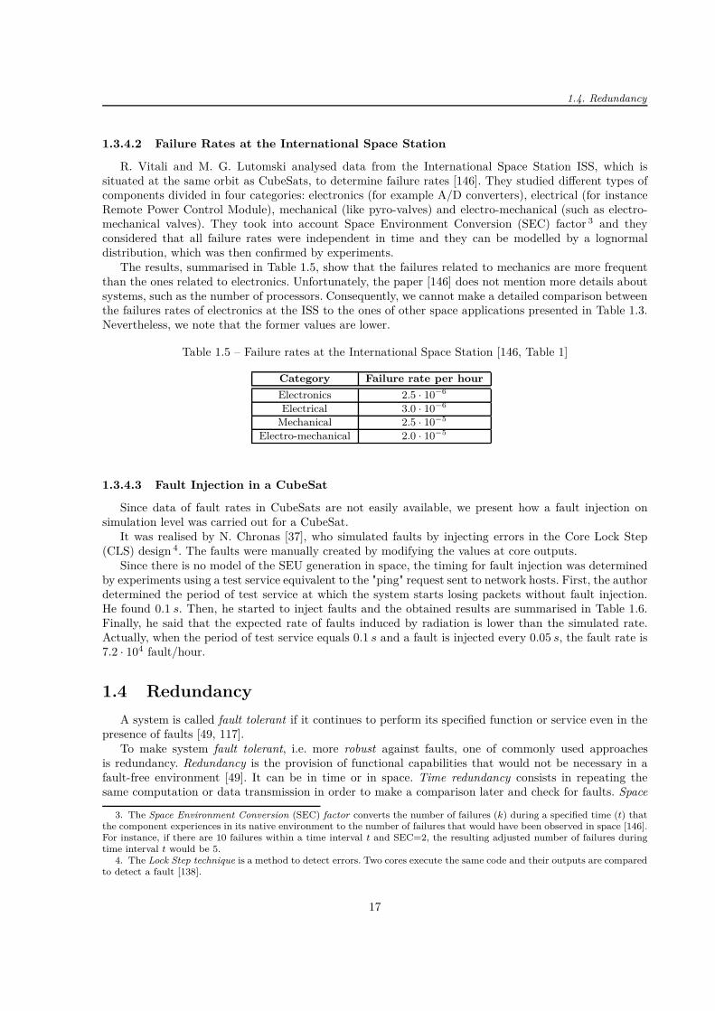
1.4. Redundancy

1.3.4.2 Failure Rates at the International Space Station

R. Vitali and M. G. Lutomski analysed data from the International Space Station ISS, which issituated at the same orbit as CubeSats, to determine failure rates [146]. They studied different types ofcomponents divided in four categories: electronics (for example A/D converters), electrical (for instanceRemote Power Control Module), mechanical (like pyro-valves) and electro-mechanical (such as electro-mechanical valves). They took into account Space Environment Conversion (SEC) factor 3 and theyconsidered that all failure rates were independent in time and they can be modelled by a lognormaldistribution, which was then confirmed by experiments.

The results, summarised in Table 1.5, show that the failures related to mechanics are more frequentthan the ones related to electronics. Unfortunately, the paper [146] does not mention more details aboutsystems, such as the number of processors. Consequently, we cannot make a detailed comparison betweenthe failures rates of electronics at the ISS to the ones of other space applications presented in Table 1.3.Nevertheless, we note that the former values are lower.

Table 1.5 – Failure rates at the International Space Station [146, Table 1]

Category Failure rate per hour

Electronics 2.5 · 10−6

Electrical 3.0 · 10−6

Mechanical 2.5 · 10−5

Electro-mechanical 2.0 · 10−5

1.3.4.3 Fault Injection in a CubeSat

Since data of fault rates in CubeSats are not easily available, we present how a fault injection onsimulation level was carried out for a CubeSat.

It was realised by N. Chronas [37], who simulated faults by injecting errors in the Core Lock Step(CLS) design 4. The faults were manually created by modifying the values at core outputs.

Since there is no model of the SEU generation in space, the timing for fault injection was determinedby experiments using a test service equivalent to the "ping" request sent to network hosts. First, the authordetermined the period of test service at which the system starts losing packets without fault injection.He found 0.1 s. Then, he started to inject faults and the obtained results are summarised in Table 1.6.Finally, he said that the expected rate of faults induced by radiation is lower than the simulated rate.Actually, when the period of test service equals 0.1 s and a fault is injected every 0.05 s, the fault rate is7.2 · 104 fault/hour.

1.4 Redundancy

A system is called fault tolerant if it continues to perform its specified function or service even in thepresence of faults [49, 117].

To make system fault tolerant, i.e. more robust against faults, one of commonly used approachesis redundancy. Redundancy is the provision of functional capabilities that would not be necessary in afault-free environment [49]. It can be in time or in space. Time redundancy consists in repeating thesame computation or data transmission in order to make a comparison later and check for faults. Space

3. The Space Environment Conversion (SEC) factor converts the number of failures (k) during a specified time (t) thatthe component experiences in its native environment to the number of failures that would have been observed in space [146].For instance, if there are 10 failures within a time interval t and SEC=2, the resulting adjusted number of failures duringtime interval t would be 5.

4. The Lock Step technique is a method to detect errors. Two cores execute the same code and their outputs are comparedto detect a fault [138].

17

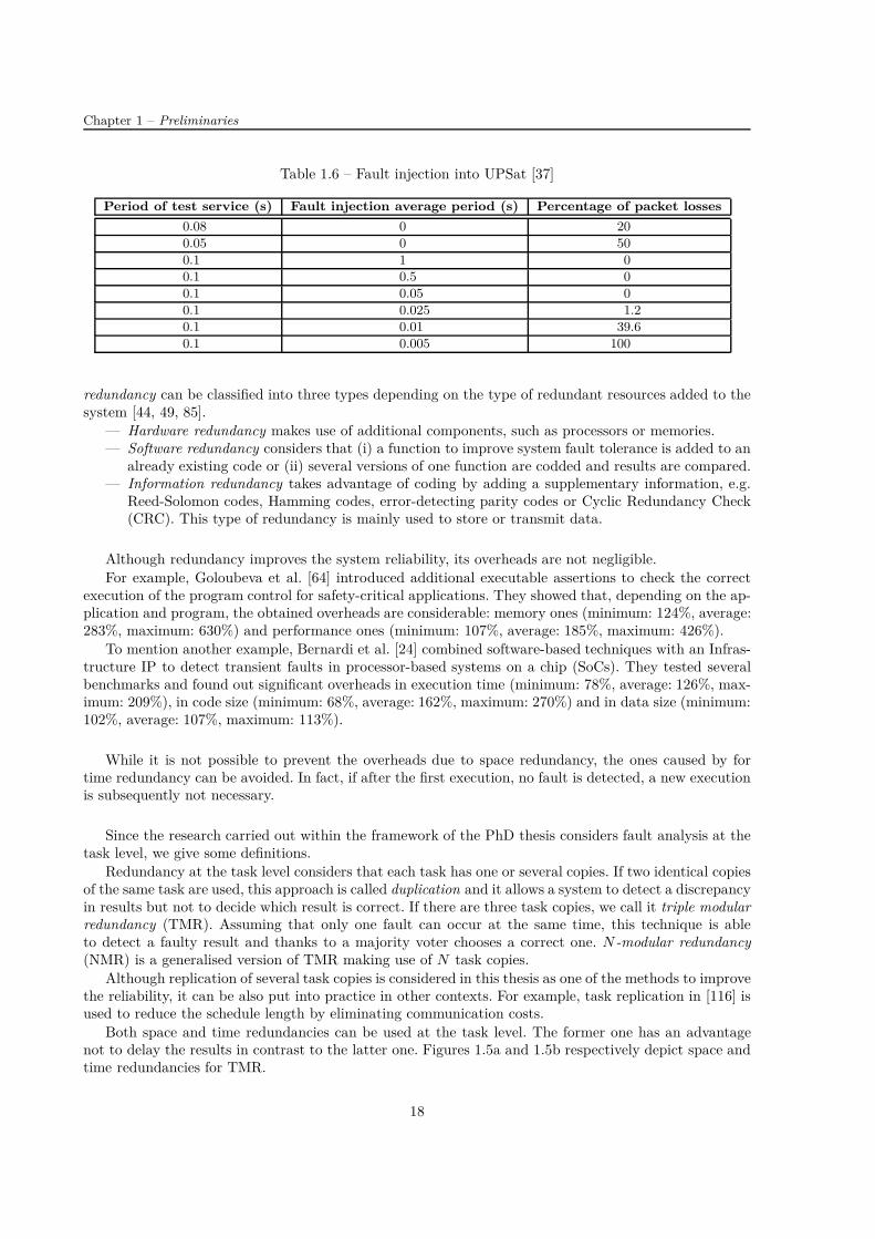
Chapter 1 – Preliminaries

Table 1.6 – Fault injection into UPSat [37]

Period of test service (s) Fault injection average period (s) Percentage of packet losses

0.08 0 20

0.05 0 50

0.1 1 0

0.1 0.5 0

0.1 0.05 0

0.1 0.025 1.2

0.1 0.01 39.6

0.1 0.005 100

redundancy can be classified into three types depending on the type of redundant resources added to thesystem [44, 49, 85].

— Hardware redundancy makes use of additional components, such as processors or memories.— Software redundancy considers that (i) a function to improve system fault tolerance is added to an

already existing code or (ii) several versions of one function are codded and results are compared.— Information redundancy takes advantage of coding by adding a supplementary information, e.g.

Reed-Solomon codes, Hamming codes, error-detecting parity codes or Cyclic Redundancy Check(CRC). This type of redundancy is mainly used to store or transmit data.

Although redundancy improves the system reliability, its overheads are not negligible.For example, Goloubeva et al. [64] introduced additional executable assertions to check the correct

execution of the program control for safety-critical applications. They showed that, depending on the ap-plication and program, the obtained overheads are considerable: memory ones (minimum: 124%, average:283%, maximum: 630%) and performance ones (minimum: 107%, average: 185%, maximum: 426%).

To mention another example, Bernardi et al. [24] combined software-based techniques with an Infras-tructure IP to detect transient faults in processor-based systems on a chip (SoCs). They tested severalbenchmarks and found out significant overheads in execution time (minimum: 78%, average: 126%, max-imum: 209%), in code size (minimum: 68%, average: 162%, maximum: 270%) and in data size (minimum:102%, average: 107%, maximum: 113%).

While it is not possible to prevent the overheads due to space redundancy, the ones caused by fortime redundancy can be avoided. In fact, if after the first execution, no fault is detected, a new executionis subsequently not necessary.

Since the research carried out within the framework of the PhD thesis considers fault analysis at thetask level, we give some definitions.

Redundancy at the task level considers that each task has one or several copies. If two identical copiesof the same task are used, this approach is called duplication and it allows a system to detect a discrepancyin results but not to decide which result is correct. If there are three task copies, we call it triple modularredundancy (TMR). Assuming that only one fault can occur at the same time, this technique is ableto detect a faulty result and thanks to a majority voter chooses a correct one. N -modular redundancy(NMR) is a generalised version of TMR making use of N task copies.

Although replication of several task copies is considered in this thesis as one of the methods to improvethe reliability, it can be also put into practice in other contexts. For example, task replication in [116] isused to reduce the schedule length by eliminating communication costs.

Both space and time redundancies can be used at the task level. The former one has an advantagenot to delay the results in contrast to the latter one. Figures 1.5a and 1.5b respectively depict space andtime redundancies for TMR.

18

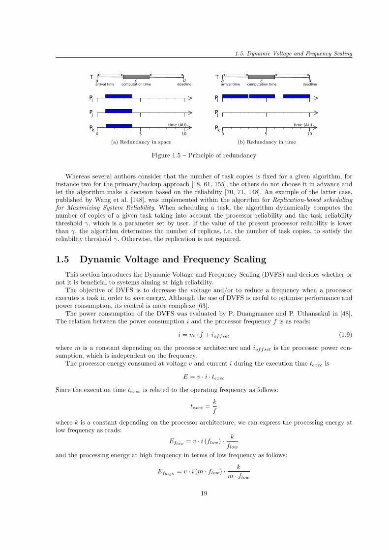
1.5. Dynamic Voltage and Frequency Scaling

(a) Redundancy in space (b) Redundancy in time

Figure 1.5 – Principle of redundancy

Whereas several authors consider that the number of task copies is fixed for a given algorithm, forinstance two for the primary/backup approach [18, 61, 155], the others do not choose it in advance andlet the algorithm make a decision based on the reliability [70, 71, 148]. An example of the latter case,published by Wang et al. [148], was implemented within the algorithm for Replication-based schedulingfor Maximizing System Reliability. When scheduling a task, the algorithm dynamically computes thenumber of copies of a given task taking into account the processor reliability and the task reliabilitythreshold γ, which is a parameter set by user. If the value of the present processor reliability is lowerthan γ, the algorithm determines the number of replicas, i.e. the number of task copies, to satisfy thereliability threshold γ. Otherwise, the replication is not required.

1.5 Dynamic Voltage and Frequency Scaling

This section introduces the Dynamic Voltage and Frequency Scaling (DVFS) and decides whether ornot it is beneficial to systems aiming at high reliability.

The objective of DVFS is to decrease the voltage and/or to reduce a frequency when a processorexecutes a task in order to save energy. Although the use of DVFS is useful to optimise performance andpower consumption, its control is more complexe [63].

The power consumption of the DVFS was evaluated by P. Duangmanee and P. Uthansakul in [48].The relation between the power consumption i and the processor frequency f is as reads:

i = m · f + ioffset (1.9)

where m is a constant depending on the processor architecture and ioffset is the processor power con-sumption, which is independent on the frequency.

The processor energy consumed at voltage v and current i during the execution time texec is

E = v · i · texec

Since the execution time texec is related to the operating frequency as follows:

texec =k

f

where k is a constant depending on the processor architecture, we can express the processing energy atlow frequency as reads:

Eflow= v · i (flow) · k

flow

and the processing energy at high frequency in terms of low frequency as follows:

Efhigh= v · i (m · flow) · k

m · flow

19

Chapter 1 – Preliminaries

The comparison of the energy consumed at high frequency Efhighto the one at low frequency Eflow

gives:

Efhigh< Eflow

⇔ v · i (m · flow) · k

m · flow< v · i (flow) · k

flow

⇔ i (m · flow)m · flow

<i (flow)

flow

⇔ m · flow + ioffset

m · flow<

flow + ioffset

flowusing Formula 1.9

⇔ 1 +ioffset

m · flow< 1 +

ioffset

flow

Since ioffset

m·flow<

ioffset

flow, the energy consumed at high frequency Efhigh

is lower than the one at lowfrequency Eflow

. It means that, at reduced frequency, the task execution is longer and the power con-sumption is higher due to static and frequency-independent energy [157].

From the point of view of the system reliability, when the frequency reduces and/or the voltagedecreases, the occurrence of transient faults increases [70, 128, 153]. It was found [153, 157, 158] that itis difficult for an algorithm using the DVFS to optimise both reliability and power consumption at thesame time. Actually, if the algorithm does not consider the reliability, the probability of failure is higher,whereas if it takes into account the reliability, the power consumption increases.

Finally, Xu et al. stated [153] that, when processors have high fault rates and any algorithm wouldhardly reduce the processor execution frequency, the algorithm without the DVFS generates the leastenergy consumption.

To conclude, the reliability and energy constraints act in the opposite manners because the improve-ment of one criterion degrades the other. All in all, the technique of the DVFS during task execution willnot be considered in this manuscript.

1.6 Summary

This chapter presented several topics to introduce the reader to the context of the PhD thesis.Firstly, system, algorithm and task classifications were given and, in particular, Graham’s 3-field

notation was presented. It will be used to classify our proposed algorithms.Secondly, we clearly defined fault, error and failure.Thirdly, we presented various tools to model faults and a processor failure rate. Fault rates for both

space and no-space applications were compared.Fourthly, we described redundancy, which is a commonly used technique to provide systems with fault

tolerance.And fifthly, we discussed the dynamic voltage and frequency scaling and concluded that we will not

make use of this technique in this thesis.

20

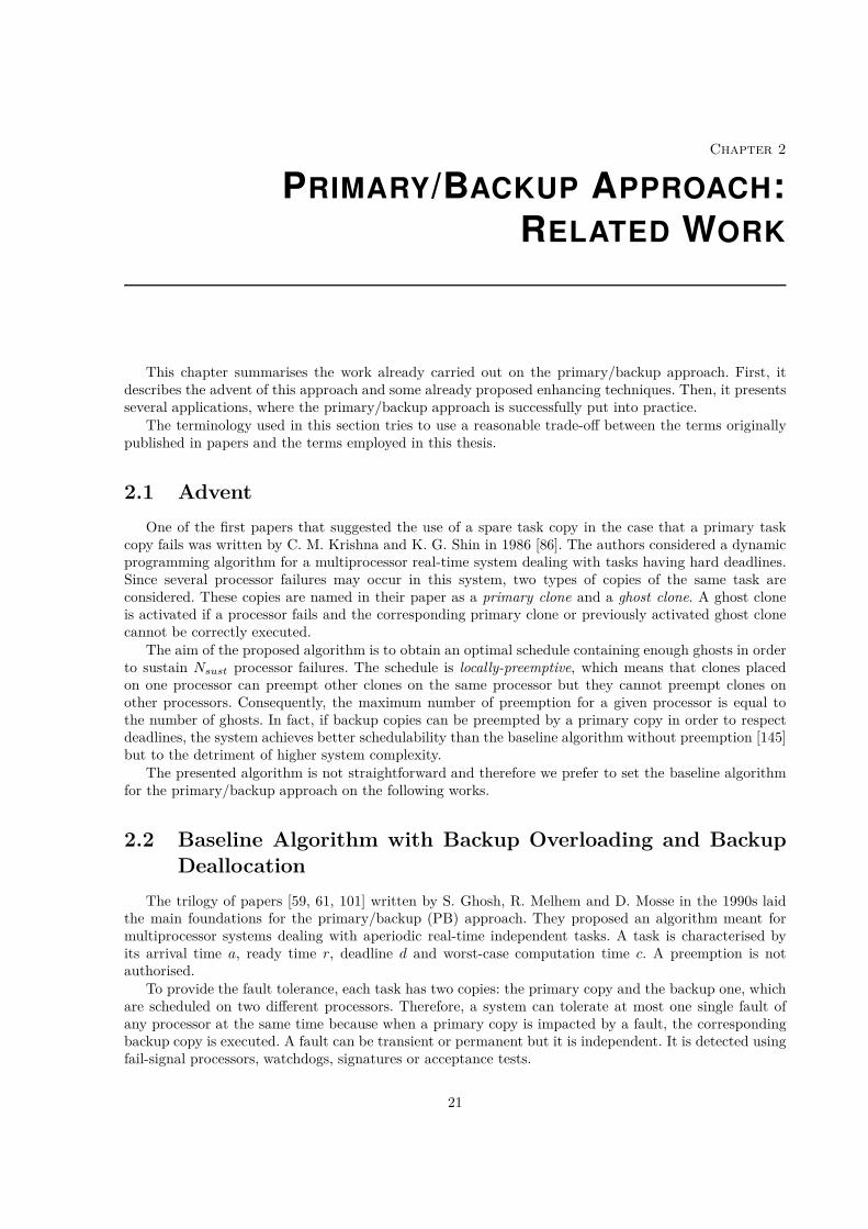
Chapter 2

PRIMARY/BACKUP APPROACH:RELATED WORK

This chapter summarises the work already carried out on the primary/backup approach. First, itdescribes the advent of this approach and some already proposed enhancing techniques. Then, it presentsseveral applications, where the primary/backup approach is successfully put into practice.

The terminology used in this section tries to use a reasonable trade-off between the terms originallypublished in papers and the terms employed in this thesis.

2.1 Advent

One of the first papers that suggested the use of a spare task copy in the case that a primary taskcopy fails was written by C. M. Krishna and K. G. Shin in 1986 [86]. The authors considered a dynamicprogramming algorithm for a multiprocessor real-time system dealing with tasks having hard deadlines.Since several processor failures may occur in this system, two types of copies of the same task areconsidered. These copies are named in their paper as a primary clone and a ghost clone. A ghost cloneis activated if a processor fails and the corresponding primary clone or previously activated ghost clonecannot be correctly executed.

The aim of the proposed algorithm is to obtain an optimal schedule containing enough ghosts in orderto sustain Nsust processor failures. The schedule is locally-preemptive, which means that clones placedon one processor can preempt other clones on the same processor but they cannot preempt clones onother processors. Consequently, the maximum number of preemption for a given processor is equal tothe number of ghosts. In fact, if backup copies can be preempted by a primary copy in order to respectdeadlines, the system achieves better schedulability than the baseline algorithm without preemption [145]but to the detriment of higher system complexity.

The presented algorithm is not straightforward and therefore we prefer to set the baseline algorithmfor the primary/backup approach on the following works.

2.2 Baseline Algorithm with Backup Overloading and BackupDeallocation

The trilogy of papers [59, 61, 101] written by S. Ghosh, R. Melhem and D. Mosse in the 1990s laidthe main foundations for the primary/backup (PB) approach. They proposed an algorithm meant formultiprocessor systems dealing with aperiodic real-time independent tasks. A task is characterised byits arrival time a, ready time r, deadline d and worst-case computation time c. A preemption is notauthorised.

To provide the fault tolerance, each task has two copies: the primary copy and the backup one, whichare scheduled on two different processors. Therefore, a system can tolerate at most one single fault ofany processor at the same time because when a primary copy is impacted by a fault, the correspondingbackup copy is executed. A fault can be transient or permanent but it is independent. It is detected usingfail-signal processors, watchdogs, signatures or acceptance tests.

21

Chapter 2 – Primary/Backup Approach: Related Work

In general, primary copies are scheduled as early as possible and backup copies are placed as late aspossible because primary copies are always executed and backup copies may not be necessary. Figure 2.1depicts an example of scheduling of task Ti (with the assumption made by the authors that ai = ri). If atask cannot be scheduled between its arrival time and the deadline, i.e. there is not enough time to placeits primary and backup copies, it is rejected.

Figure 2.1 – Example of scheduling one task

In order to improve the schedulability and increase the processor utilisation two improving techniqueswere proposed: the backup overloading and backup deallocation. The backup overloading authorises sev-eral backup copies, if their respective primary copies are not scheduled on the same processor, to beoverloaded, i.e. to share the same time slots on a processor, because only one backup copy will be neces-sary, if a fault occurs. An example of this technique is illustrated in Figure 2.2.

Figure 2.2 – Example of backup overloading

The backup deallocation means that a backup copy frees its slot once the corresponding primary copyis correctly executed.

The authors showed a dilemma of a scheduling choice for two aforementioned techniques. To favourthe backup overloading, backup copies should be placed so that they overlap as much as possible, which isnot necessarily as late as possible. To determine which technique is more effective, they chose the schedulemaximizing the cost function Φ defined as follows:

Φ = (Start time of backup copy) + ω · (Overlap length) (2.1)

where the first addend is related to the backup deallocation and the second one is related to the backupoverloading. The positive value of ω is fixed by user to set the prevalence of one of the aforementionedto another.

When introducing simple improvements for the primary/backup approach, we also mention that G.Manimaran and C. S. R. Murthy introduced resource reclaiming [96] in order to free slots when there arenot necessary any more because a task copy finishes its execution earlier than originally scheduled.

22

2.3. Processor Allocation Policy

To evaluate the system performances, the authors made use of two metrics. The rejection ratio ac-counting for the percentage of arriving tasks rejected by the system. The second metric is related to thesystem resiliency and called the time to second fault. It is the time it takes for the system to be able totolerate a second fault after the first fault occurs.

The results show that; to reduce the rejection ratio, it is necessary to reduce the processor load, toadd additional processors and/or to increase the window ratio (defined as wri = di−ri

ci). The time to

second fault is longer when the number of processors decreases and/or the window ratio increases. Whenthe primary/backup approach is compared to the system having a spare processor on which all backupcopies are scheduled, its schedulability is higher due to better resource utilisation.

It was shown that both the backup deallocation and the backup overloading reduce the rejection ratio.Nevertheless, the backup deallocation performs better than the backup overloading because it is moreadvantageous freeing a slot on a processor than overloading already existing backup copies.

Finally, the authors noted that to handle multiple simultaneous faults it would be necessary to schedulemore than one backup copies for each task, which will improve the system resiliency but to the detrimentof overheads.

2.3 Processor Allocation Policy

When scheduling a new task and searching for a free slot, the choice of processor allocation policyplays an important role because it has a significant bearing on the system performances, such as therejection rate or algorithm run-time. This section describes four types of searches: random, exhaustive,sequential and load-based.

2.3.1 Random Search

The random search randomly chooses one processor on which the algorithm tries to find a free slot[104]. A free slot is a time interval of processor schedule not occupied by any task copy and where a taskcopy of a new task can be placed. If a task copy is not placed on the first randomly chosen processor, aschedule of other randomly chosen processor is considered and so forth until the algorithm exhausts allpossibilities or finds a free slot large enough to accommodate a task copy. The search is similar for bothprimary and backup copies.

2.3.2 Exhaustive Search

The exhaustive search was put into practice in the baseline approach presented in Section 2.2 [59, 61,101]. This allocation policy tests all (P ) processors to find a free slot as soon as possible for primary copyand (P − 1) processors to search for a free slot as late as possible for backup copy. Algorithm 1 sums upthe main steps of the exhaustive search.

23

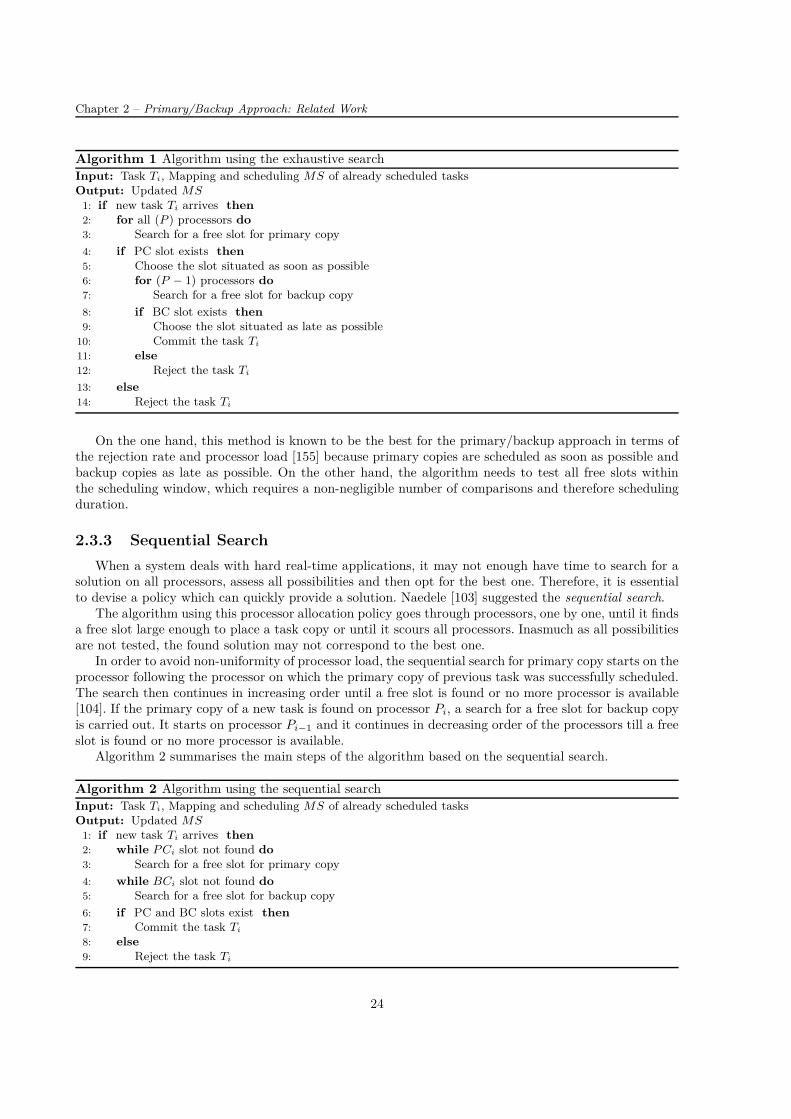
Chapter 2 – Primary/Backup Approach: Related Work

Algorithm 1 Algorithm using the exhaustive searchInput: Task Ti, Mapping and scheduling MS of already scheduled tasksOutput: Updated MS

1: if new task Ti arrives then2: for all (P ) processors do3: Search for a free slot for primary copy

4: if PC slot exists then5: Choose the slot situated as soon as possible6: for (P − 1) processors do7: Search for a free slot for backup copy

8: if BC slot exists then9: Choose the slot situated as late as possible

10: Commit the task Ti

11: else12: Reject the task Ti

13: else14: Reject the task Ti

On the one hand, this method is known to be the best for the primary/backup approach in terms ofthe rejection rate and processor load [155] because primary copies are scheduled as soon as possible andbackup copies as late as possible. On the other hand, the algorithm needs to test all free slots withinthe scheduling window, which requires a non-negligible number of comparisons and therefore schedulingduration.

2.3.3 Sequential Search

When a system deals with hard real-time applications, it may not enough have time to search for asolution on all processors, assess all possibilities and then opt for the best one. Therefore, it is essentialto devise a policy which can quickly provide a solution. Naedele [103] suggested the sequential search.

The algorithm using this processor allocation policy goes through processors, one by one, until it findsa free slot large enough to place a task copy or until it scours all processors. Inasmuch as all possibilitiesare not tested, the found solution may not correspond to the best one.

In order to avoid non-uniformity of processor load, the sequential search for primary copy starts on theprocessor following the processor on which the primary copy of previous task was successfully scheduled.The search then continues in increasing order until a free slot is found or no more processor is available[104]. If the primary copy of a new task is found on processor Pi, a search for a free slot for backup copyis carried out. It starts on processor Pi−1 and it continues in decreasing order of the processors till a freeslot is found or no more processor is available.

Algorithm 2 summarises the main steps of the algorithm based on the sequential search.

Algorithm 2 Algorithm using the sequential searchInput: Task Ti, Mapping and scheduling MS of already scheduled tasksOutput: Updated MS

1: if new task Ti arrives then2: while P Ci slot not found do3: Search for a free slot for primary copy

4: while BCi slot not found do5: Search for a free slot for backup copy

6: if PC and BC slots exist then7: Commit the task Ti

8: else9: Reject the task Ti

24

2.4. Improvements

2.3.4 Load-based Search

Naedele [104] presented also another processor allocation policy. It is based on processor load. Beforesearching for a free slot, the algorithm evaluates the current processor load and it orders processors ina list according to their increasing workload. The search then starts on the least loaded processor. Thesearch for a free slot for primary copy is carried out on odd processors and the one for backup copies isconducted on even processors until a solution is found or all possibilities are tested.

This method seems to be well applicable for dynamic mapping and scheduling [18] but its imple-mentation may require more resources and algorithm run-time than the previously mentioned processorallocation policies. When these different policies were compared, it was found out that the sequentialsearch and the load-based one have similar performances [104].

The main scheduling steps of the algorithm using the load-based search are shown in Algorithm 3.

Algorithm 3 Algorithm using the load-based searchInput: Task Ti, Mapping and scheduling MS of already scheduled tasksOutput: Updated MS

1: if new task Ti arrives then2: Order processors by their increasing load3: while P Ci slot not found do4: Search for a free slot for primary copy on odd processors

5: while BCi slot not found do6: Search for a free slot for backup copy on even processors

7: if PC and BC slots exist then8: Commit the task Ti

9: else10: Reject the task Ti

To sum up, the random processor allocation is not ingenious and the exhaustive search is more likelyto be complex. The load-based and sequential processor allocation policies achieve good results but theformer one is more complex due to system monitoring.

2.4 Improvements

We present improvements already proposed for the primary/backup approach. After the descriptionof the primary slack and decision deadline, the difference between the passive and active primary/backupapproach is explained. Finally, the computation of replication cost is introduced, as well as the boundaryschedules and the primary-backup overloading.

2.4.1 Primary Slack

A condition may sometime occur that a free slot is not large enough to accommodate a task copyxCto_be_scheduled. The solution proposed by [61] is to move forward already scheduled primary copies(without violating their time constraints) in order to increase the length of the free slot if it is not largeenough to place a copy of a new task. That is why, the primary copy P Cto_be_moved_forward, whichhinders scheduling a task copy xCto_be_scheduled, can be moved forward if there is another free slotafter xCto_be_moved_forward and if both tasks Tto_be_moved_forward and Tto_be_scheduled respect theirrespective deadlines. Ghosh et al. defined the slack, as the maximum time by which the start of a taskcan be delayed to meet its deadline.

The backup copies are not concerned by this technique because they are scheduled as late as possibleand they consequently cannot be moved forward. Moreover, several backup copies can be overloaded,which complicates the use of slack for backup copies.

25

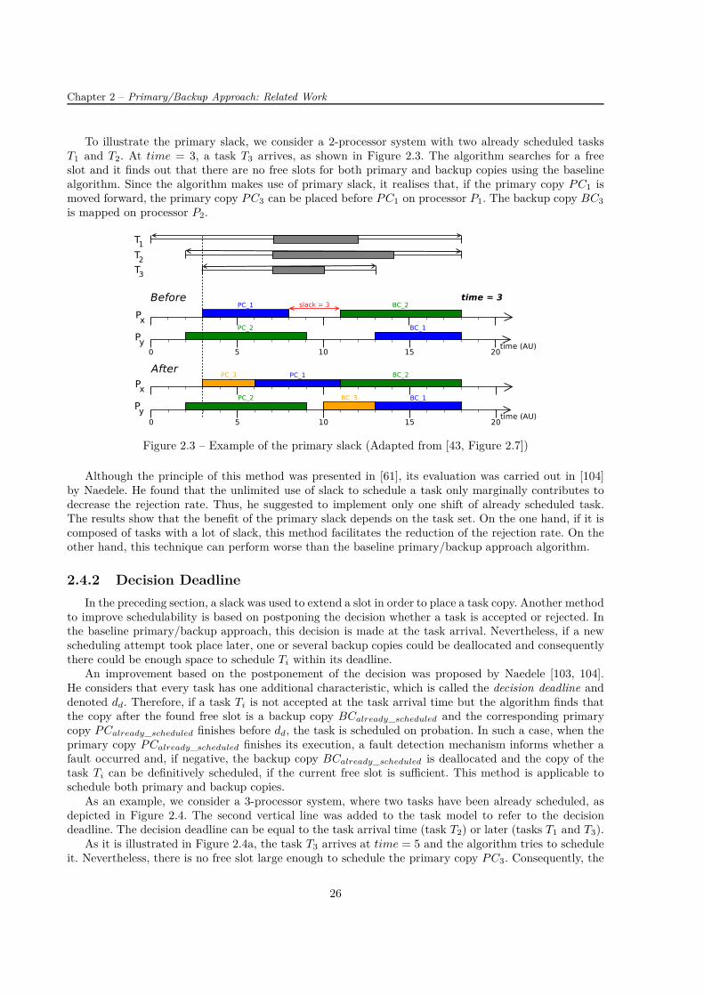
Chapter 2 – Primary/Backup Approach: Related Work

To illustrate the primary slack, we consider a 2-processor system with two already scheduled tasksT1 and T2. At time = 3, a task T3 arrives, as shown in Figure 2.3. The algorithm searches for a freeslot and it finds out that there are no free slots for both primary and backup copies using the baselinealgorithm. Since the algorithm makes use of primary slack, it realises that, if the primary copy P C1 ismoved forward, the primary copy P C3 can be placed before P C1 on processor P1. The backup copy BC3

is mapped on processor P2.

Figure 2.3 – Example of the primary slack (Adapted from [43, Figure 2.7])

Although the principle of this method was presented in [61], its evaluation was carried out in [104]by Naedele. He found that the unlimited use of slack to schedule a task only marginally contributes todecrease the rejection rate. Thus, he suggested to implement only one shift of already scheduled task.The results show that the benefit of the primary slack depends on the task set. On the one hand, if it iscomposed of tasks with a lot of slack, this method facilitates the reduction of the rejection rate. On theother hand, this technique can perform worse than the baseline primary/backup approach algorithm.

2.4.2 Decision Deadline

In the preceding section, a slack was used to extend a slot in order to place a task copy. Another methodto improve schedulability is based on postponing the decision whether a task is accepted or rejected. Inthe baseline primary/backup approach, this decision is made at the task arrival. Nevertheless, if a newscheduling attempt took place later, one or several backup copies could be deallocated and consequentlythere could be enough space to schedule Ti within its deadline.

An improvement based on the postponement of the decision was proposed by Naedele [103, 104].He considers that every task has one additional characteristic, which is called the decision deadline anddenoted dd. Therefore, if a task Ti is not accepted at the task arrival time but the algorithm finds thatthe copy after the found free slot is a backup copy BCalready_scheduled and the corresponding primarycopy P Calready_scheduled finishes before dd, the task is scheduled on probation. In such a case, when theprimary copy P Calready_scheduled finishes its execution, a fault detection mechanism informs whether afault occurred and, if negative, the backup copy BCalready_scheduled is deallocated and the copy of thetask Ti can be definitively scheduled, if the current free slot is sufficient. This method is applicable toschedule both primary and backup copies.

As an example, we consider a 3-processor system, where two tasks have been already scheduled, asdepicted in Figure 2.4. The second vertical line was added to the task model to refer to the decisiondeadline. The decision deadline can be equal to the task arrival time (task T2) or later (tasks T1 and T3).

As it is illustrated in Figure 2.4a, the task T3 arrives at time = 5 and the algorithm tries to scheduleit. Nevertheless, there is no free slot large enough to schedule the primary copy P C3. Consequently, the

26

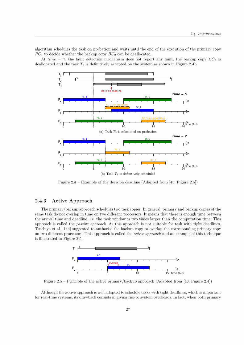
2.4. Improvements

algorithm schedules the task on probation and waits until the end of the execution of the primary copyP C1 to decide whether the backup copy BC2 can be deallocated.

At time = 7, the fault detection mechanism does not report any fault, the backup copy BC2 isdeallocated and the task T3 is definitively accepted on the system as shown in Figure 2.4b.

(a) Task T3 is scheduled on probation

(b) Task T3 is definitively scheduled

Figure 2.4 – Example of the decision deadline (Adapted from [43, Figure 2.5])

2.4.3 Active Approach

The primary/backup approach schedules two task copies. In general, primary and backup copies of thesame task do not overlap in time on two different processors. It means that there is enough time betweenthe arrival time and deadline, i.e. the task window is two times larger than the computation time. Thisapproach is called the passive approach. As this approach is not suitable for task with tight deadlines,Tsuchiya et al. [144] suggested to authorise the backup copy to overlap the corresponding primary copyon two different processors. This approach is called the active approach and an example of this techniqueis illustrated in Figure 2.5.

Figure 2.5 – Principle of the active primary/backup approach (Adapted from [43, Figure 2.4])

Although the active approach is well adapted to schedule tasks with tight deadlines, which is importantfor real-time systems, its drawback consists in giving rise to system overheads. In fact, when both primary

27

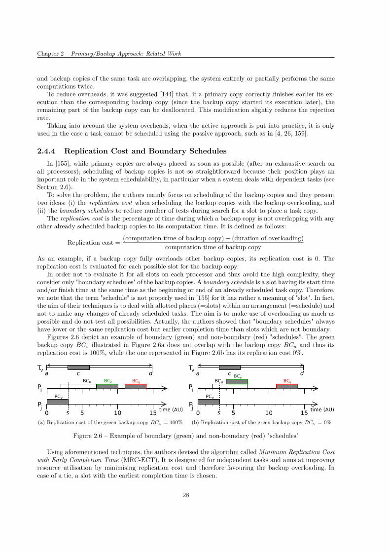
Chapter 2 – Primary/Backup Approach: Related Work

and backup copies of the same task are overlapping, the system entirely or partially performs the samecomputations twice.

To reduce overheads, it was suggested [144] that, if a primary copy correctly finishes earlier its ex-ecution than the corresponding backup copy (since the backup copy started its execution later), theremaining part of the backup copy can be deallocated. This modification slightly reduces the rejectionrate.

Taking into account the system overheads, when the active approach is put into practice, it is onlyused in the case a task cannot be scheduled using the passive approach, such as in [4, 26, 159].

2.4.4 Replication Cost and Boundary Schedules

In [155], while primary copies are always placed as soon as possible (after an exhaustive search onall processors), scheduling of backup copies is not so straightforward because their position plays animportant role in the system schedulability, in particular when a system deals with dependent tasks (seeSection 2.6).

To solve the problem, the authors mainly focus on scheduling of the backup copies and they presenttwo ideas: (i) the replication cost when scheduling the backup copies with the backup overloading, and(ii) the boundary schedules to reduce number of tests during search for a slot to place a task copy.

The replication cost is the percentage of time during which a backup copy is not overlapping with anyother already scheduled backup copies to its computation time. It is defined as follows:

Replication cost =(computation time of backup copy) − (duration of overloading)

computation time of backup copy

As an example, if a backup copy fully overloads other backup copies, its replication cost is 0. Thereplication cost is evaluated for each possible slot for the backup copy.

In order not to evaluate it for all slots on each processor and thus avoid the high complexity, theyconsider only "boundary schedules" of the backup copies. A boundary schedule is a slot having its start timeand/or finish time at the same time as the beginning or end of an already scheduled task copy. Therefore,we note that the term "schedule" is not properly used in [155] for it has rather a meaning of "slot". In fact,the aim of their techniques is to deal with allotted places (=slots) within an arrangement (=schedule) andnot to make any changes of already scheduled tasks. The aim is to make use of overloading as much aspossible and do not test all possibilities. Actually, the authors showed that "boundary schedules" alwayshave lower or the same replication cost but earlier completion time than slots which are not boundary.

Figures 2.6 depict an example of boundary (green) and non-boundary (red) "schedules". The greenbackup copy BCv illustrated in Figure 2.6a does not overlap with the backup copy BCu and thus itsreplication cost is 100%, while the one represented in Figure 2.6b has its replication cost 0%.

(a) Replication cost of the green backup copy BCv = 100% (b) Replication cost of the green backup copy BCv = 0%

Figure 2.6 – Example of boundary (green) and non-boundary (red) "schedules"

Using aforementioned techniques, the authors devised the algorithm called Minimum Replication Costwith Early Completion Time (MRC-ECT). It is designated for independent tasks and aims at improvingresource utilisation by minimising replication cost and therefore favouring the backup overloading. Incase of a tie, a slot with the earliest completion time is chosen.

28

2.4. Improvements

On the one hand, the results show that the proposed algorithm rejects less tasks and has lowerreplication cost than the algorithm scheduling all backup copies as soon as possible. On the other hand,the response time of the backup copies, i.e. the time when results are available, is longer.

Inspired by these enhancements, J. Balasangameshwara and N. Raju [18] proposed a fault tolerantload-balancing algorithm aiming at reducing replication cost and completion time. The algorithm isdynamic, adaptive and decentralised, which means that all system resources contribute to balance thesystem load. The resource load at a given time instant is defined as the total length of the jobs in thequeue, where tasks are waiting to be executed, divided by the current capacity of the resource.

The authors consider a heterogeneous system dealing with independent tasks only. The devised algo-rithm takes into account communication costs among resources, such as transfer delay and data trans-mission rate, and can tolerate transient and permanent faults assumed to be independent. Regarding thefault model, the authors consider a fault-detection mechanism to detect faults and that only one versionof a job, i.e. one job copy, can encounter a fault.

In order to evaluate the resource load, the authors propose a resource efficiency estimation policy,which means that each submitted but not yet executed job adds one point to the resource score and whenit is executed one point is deducted. The lower the resource score, the higher the resource efficiency.

The goal of the load adjustment policy is to reduce the difference in load among resources by taskmigration. A task can migrate if it is waiting in a queue and other resource is less charged. To limit thetask migration and avoid burdening several resources, the authors define a threshold for the maximumexchange in the system.

Other improvement proposed in this paper is the refinement of the mutual information feedback byadding information concerning the efficiency. Thus, each resource is aware of state (load and efficiency)of its neighbouring resources. These data are approximate because, in order to reduce communicationcosts, there is no message exchange unless there is a task transfer request between resources to whichthese data are appended.

The proposed algorithm guarantees to find an optimal backup slot, which reduces replication costand thus contributes to higher utilisation efficiency but at the cost of testing all resources (1000 in theirexperiments). It was shown that a resource should exchange state message with only several neighbouringresources in order not to increase the response time. Furthermore, when the load increases, the averageresponse time increases and the replication cost remains stable. Finally, the system fault tolerance isindependent of the system heterogeneity and of the number of jobs in one job set.

2.4.5 Primary-Backup Overloading

In many papers, the authors assume that there is only one fault in the system at the same time.Consequently, when using the primary/backup approach with the backup overloading, several backupcopies can overlap each other because only one copy will be executed in case of a fault occurrence.

R. Al-Omari et al., inspired by the backup overloading, proposed the primary-backup overloadingto improve the schedulability in the multiprocessor real-time systems [5]. This technique requires thebackup deallocation and authorises a primary copy of one task to overlap a backup copy of another task.Therefore, it is necessary to distinguish two states of the backup copies based on whether or not a backupcopy takes part in the primary-backup overloading and subsequently cannot be overloaded anymore. Thechanges of states of the backup copies are encapsulated in Algorithm 4 and they are respectively denotedP B_overload_authorised and P B_overload_forbidden [43].

To illustrate the primary-backup overloading, an example is depicted in Figure 2.7a. At time = 6, weconsider a 3-processor system having three already scheduled tasks, when a task T4 arrives. Its primarycopy is scheduled on the processor P1 where it overlaps with the backup copy of the task T1. We note thatit would not be possible to schedule the task T4 without the primary-backup overloading. At time = 7,there are two possibilities:

1. The primary copy P C1 is correctly executed and the backup copy BC1 is deallocated. Thus, theprimary copy P C4 can continue its execution. This scenario is illustrated in Figure 2.7b.

29

Chapter 2 – Primary/Backup Approach: Related Work

Algorithm 4 Implementation of the primary-backup overloading1: if primary copy P Ci has just been scheduled then2: if P Ci is scheduled without overloading with another backup BCj then3: Update the state of BCi to P B_overload_authorised4: else5: Update the state of BCi to P B_overload_forbidden

6: if primary copy P Ck has just finished then7: if BCk overlaps with P Ci then8: if no fault occurs during P Ck then ⊲ BCk is deallocated9: Update the state of BCi to P B_overload_authorised

10: else ⊲ BCk cannot be deallocated11: Update the state of BCk to P B_overload_forbidden

2. A fault occurs during the execution of the primary copy P C1 and the system waits for the resultsof the backup copy BC1, as shown in Figure 2.7c. Subsequently, the primary copy P C4 cannot beexecuted and the result of the task T4 will be known after the execution of the backup copy BC4.

As this example shows, the primary-backup overloading increases the schedulability but at the cost ofhigher time to second fault. In [5], the authors evaluating this technique concluded that the schedulabilityis better about 25% compared to the backup overloading and that the upper bound of the time to secondfault is twice as high as the time to second fault for the backup overloading.

W. Sun et al. [142] then put together the backup overloading and the primary-backup overloadingand called it the hybrid overloading. It means that two overloading techniques jointly work to improvethe system schedulability. It was shown that the hybrid overloading achieves an acceptance ratio similarto the one of the primary-backup overloading and that the value of the time to second fault is betweenthe one for the primary-backup overloading and the one for the backup overloading.

2.5 Fault Tolerance of the Primary/Backup Approach

Although a great deal of research has been conducted on the scheduling algorithms for the prima-ry/backup approach, only few studies evaluating their resiliency have been published, despite the fact thatthis topic is of major concern for the embedded systems. In this section, we sum up several approaches.

At the beginning, no faults were injected and the system resiliency were evaluated by means of ametric called the time to second fault [61]. It is the time it takes for the system to be able to tolerate asecond fault after the first fault occurs. S. Ghosh et al. [61] considered only one transient or permanentindependent fault in the system at the same time and they showed that this time is longer when thenumber of processors decreases and/or the window ratio increases.

G. Manimaran and C. S. R. Murthy [96] associated each primary copy with the probability that thiscopy fails. The values were between 10% and 50%. They assumed that there may be more than onetransient or permanent independent faults all at once in the system because processors are divided intogroups and each group can tolerate one fault. They found that the higher the probability that the primarycopy fails, the lower the guarantee ratio.

H. Kim et al. [83] disproved a hypothesis made in [60], where the authors assumed that there is atmost one fault within time interval ∆f since this assumption is not always valid as shown in Figure 2.8a.Consequently, they stated that it is necessary to consider inter-fault time ∆F , which is the time betweenone fault that occurred and the next fault. It is depicted in Figure 2.8b. They still consider that faults aretransient or intermittent and that the system can tolerate only one fault. In their simulation, faults weregenerated with the fault rate 0.2 so that the minimum fault time ∆F = 200 (time units). The resultsshowed that the presence of faults greatly affects the rejection rate. They conducted 10 simulations andthe rejection rate varied from several percents up to 20%.

30

2.5. Fault Tolerance of the Primary/Backup Approach

(a) Primary-backup overloading of tasks T1 and T3

(b) BC1 can be deallocated

(c) BC1 cannot be deallocated

Figure 2.7 – Example of the primary-backup overloading (Adapted from [43, Figure 2.6])

(a) Fault interval ∆f (b) Minimum inter-fault time ∆F

Figure 2.8 – Difference between ∆f and ∆F (Adapted from [83, Figures 1 and 2])

Similarly to the previous work, H. Beitollahi et al. [21] injected faults based on a value of the meantime to failure (MTTF). Since this research considered only a uniprocessor system, a transient fault wasconsidered. They concluded that the larger MTTF, i.e. the lower the failure rate, the lower the numberof lost tasks.

The authors of papers [9, 122] considered only one processor permanent failure and modelled thesystem reliability as follows:

R = e−λc

where λ is a processor failure rate and c is a task computation time. As expected, they found out thatthe higher the fault rate, the lower the reliability.

31

Chapter 2 – Primary/Backup Approach: Related Work

Since faults are in general a random phenomenon in nature, R. Sridharan and R. Mahapatra [136]suggested to make use of a stochastic process to model transient faults. Thus, faults were generated usingthe Poisson distribution and injected at task level. The authors were interested in the response time,which is directly related to the energy consumption. The higher the number of faults injected, the higherthe energy consumption due to increased response time.

X. Zhu et al. [159] proposed a QoS-aware (quality of service) fault tolerant scheduling algorithmdealing with transient and permanent independent faults. At the same time, there is at most one fault.Faults were uniformly distributed with the fault rate of node equal to 10−7/h and it was shown that thereliability cost computed for the system is almost independent of the number of nodes, task arrival time,task deadline, task heterogeneity and system heterogeneity.

2.6 Dependent Tasks

In general, dependent tasks are modelled by the directed acyclic graph (DAG) G = V, E where Vstands for a set of non-preemptable tasks and E denotes a set of directed edges representing communica-tion among tasks. Every DAG is characterised by arrival time, deadline and computation time for eachtask. An example is depicted in Figure 2.9.

Figure 2.9 – An example of the general directed acyclic graph (DAG)

X. Qin and H. Jiang [121] present the efficient fault tolerant reliability-driven algorithm (eFRD), whichis an offline scheduling algorithm based on the primary/backup approach. It can deal with hard real-timenon-preemptable tasks with precedence constraints. This algorithm is reliability-aware because tasks areallocated to processors having high reliability.

The system consists of P heterogeneous processors with fully connected network. The computationalheterogeneity is represented by different task execution times on each processor in the system. It cantolerate one processor permanent fault. The authors assume that the fault arrival rate is constant andthe distribution of the fault-count for any fixed time interval is approximated using the Poisson probabilitydistribution.

The algorithm schedules the primary and backup copies as soon as possible. Both copies of the sametask can overlap neither in time nor in space. First, it searches for a primary copy slot on all processorsand it chooses the slot having the highest reliability (computed based on processor failure rates) and, incase of a tie, the earliest slot is selected. Second, it looks for a backup copy slot on all processor, except theone accommodating the corresponding primary copy, and it opts for the slot having the highest reliabilityand the earliest start time.

Regarding the proposed algorithm eFRD, the results show that the more precedence constraints amongtasks, the more messages exchanged and consequently the less task parallelism available, which has animpact on the system schedulability and reliability. Furthermore, the authors carried out simulationsusing 9 through 16 processors and they stated that the reliability and schedulability remain constantregardless of the number of processors.

In Section 2.4.4, we have already mentioned the work published in [155] regarding the replication costand boundary schedules. Q. Zheng et al. focus on online scheduling of not only independent tasks but

32

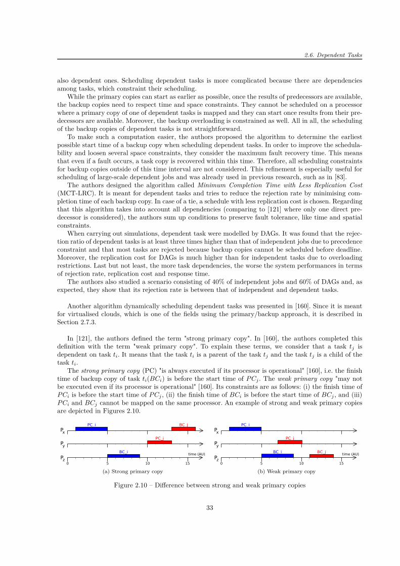
2.6. Dependent Tasks

also dependent ones. Scheduling dependent tasks is more complicated because there are dependenciesamong tasks, which constraint their scheduling.

While the primary copies can start as earlier as possible, once the results of predecessors are available,the backup copies need to respect time and space constraints. They cannot be scheduled on a processorwhere a primary copy of one of dependent tasks is mapped and they can start once results from their pre-decessors are available. Moreover, the backup overloading is constrained as well. All in all, the schedulingof the backup copies of dependent tasks is not straightforward.

To make such a computation easier, the authors proposed the algorithm to determine the earliestpossible start time of a backup copy when scheduling dependent tasks. In order to improve the schedula-bility and loosen several space constraints, they consider the maximum fault recovery time. This meansthat even if a fault occurs, a task copy is recovered within this time. Therefore, all scheduling constraintsfor backup copies outside of this time interval are not considered. This refinement is especially useful forscheduling of large-scale dependent jobs and was already used in previous research, such as in [83].

The authors designed the algorithm called Minimum Completion Time with Less Replication Cost(MCT-LRC). It is meant for dependent tasks and tries to reduce the rejection rate by minimising com-pletion time of each backup copy. In case of a tie, a schedule with less replication cost is chosen. Regardingthat this algorithm takes into account all dependencies (comparing to [121] where only one direct pre-decessor is considered), the authors sum up conditions to preserve fault tolerance, like time and spatialconstraints.

When carrying out simulations, dependent task were modelled by DAGs. It was found that the rejec-tion ratio of dependent tasks is at least three times higher than that of independent jobs due to precedenceconstraint and that most tasks are rejected because backup copies cannot be scheduled before deadline.Moreover, the replication cost for DAGs is much higher than for independent tasks due to overloadingrestrictions. Last but not least, the more task dependencies, the worse the system performances in termsof rejection rate, replication cost and response time.

The authors also studied a scenario consisting of 40% of independent jobs and 60% of DAGs and, asexpected, they show that its rejection rate is between that of independent and dependent tasks.

Another algorithm dynamically scheduling dependent tasks was presented in [160]. Since it is meantfor virtualised clouds, which is one of the fields using the primary/backup approach, it is described inSection 2.7.3.

In [121], the authors defined the term "strong primary copy". In [160], the authors completed thisdefinition with the term "weak primary copy". To explain these terms, we consider that a task tj isdependent on task ti. It means that the task ti is a parent of the task tj and the task tj is a child of thetask ti.

The strong primary copy (PC) "is always executed if its processor is operational" [160], i.e. the finishtime of backup copy of task ti(BCi) is before the start time of P Cj . The weak primary copy "may notbe executed even if its processor is operational" [160]. Its constraints are as follows: (i) the finish time ofP Ci is before the start time of P Cj , (ii) the finish time of BCi is before the start time of BCj , and (iii)P Ci and BCj cannot be mapped on the same processor. An example of strong and weak primary copiesare depicted in Figures 2.10.

(a) Strong primary copy (b) Weak primary copy

Figure 2.10 – Difference between strong and weak primary copies

33

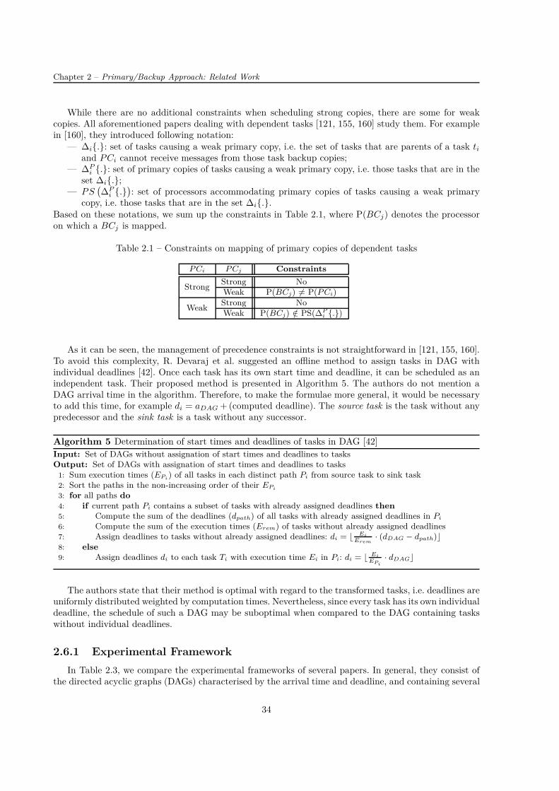
Chapter 2 – Primary/Backup Approach: Related Work

While there are no additional constraints when scheduling strong copies, there are some for weakcopies. All aforementioned papers dealing with dependent tasks [121, 155, 160] study them. For examplein [160], they introduced following notation:

— ∆i.: set of tasks causing a weak primary copy, i.e. the set of tasks that are parents of a task ti

and P Ci cannot receive messages from those task backup copies;— ∆P

i .: set of primary copies of tasks causing a weak primary copy, i.e. those tasks that are in theset ∆i.;

— P S(

∆Pi .

)

: set of processors accommodating primary copies of tasks causing a weak primarycopy, i.e. those tasks that are in the set ∆i..

Based on these notations, we sum up the constraints in Table 2.1, where P(BCj) denotes the processoron which a BCj is mapped.

Table 2.1 – Constraints on mapping of primary copies of dependent tasks

P Ci P Cj Constraints

StrongStrong NoWeak P(BCj) 6= P(P Ci)

WeakStrong NoWeak P(BCj) /∈ PS(∆P

i .)

As it can be seen, the management of precedence constraints is not straightforward in [121, 155, 160].To avoid this complexity, R. Devaraj et al. suggested an offline method to assign tasks in DAG withindividual deadlines [42]. Once each task has its own start time and deadline, it can be scheduled as anindependent task. Their proposed method is presented in Algorithm 5. The authors do not mention aDAG arrival time in the algorithm. Therefore, to make the formulae more general, it would be necessaryto add this time, for example di = aDAG + (computed deadline). The source task is the task without anypredecessor and the sink task is a task without any successor.

Algorithm 5 Determination of start times and deadlines of tasks in DAG [42]Input: Set of DAGs without assignation of start times and deadlines to tasksOutput: Set of DAGs with assignation of start times and deadlines to tasks

1: Sum execution times (EPi) of all tasks in each distinct path Pi from source task to sink task2: Sort the paths in the non-increasing order of their EPi

3: for all paths do4: if current path Pi contains a subset of tasks with already assigned deadlines then5: Compute the sum of the deadlines (dpath) of all tasks with already assigned deadlines in Pi

6: Compute the sum of the execution times (Erem) of tasks without already assigned deadlines7: Assign deadlines to tasks without already assigned deadlines: di = ⌊ Ei

Erem· (dDAG − dpath)⌋

8: else9: Assign deadlines di to each task Ti with execution time Ei in Pi: di = ⌊ Ei

EPi

· dDAG⌋

The authors state that their method is optimal with regard to the transformed tasks, i.e. deadlines areuniformly distributed weighted by computation times. Nevertheless, since every task has its own individualdeadline, the schedule of such a DAG may be suboptimal when compared to the DAG containing taskswithout individual deadlines.

2.6.1 Experimental Framework

In Table 2.3, we compare the experimental frameworks of several papers. In general, they consist ofthe directed acyclic graphs (DAGs) characterised by the arrival time and deadline, and containing several

34

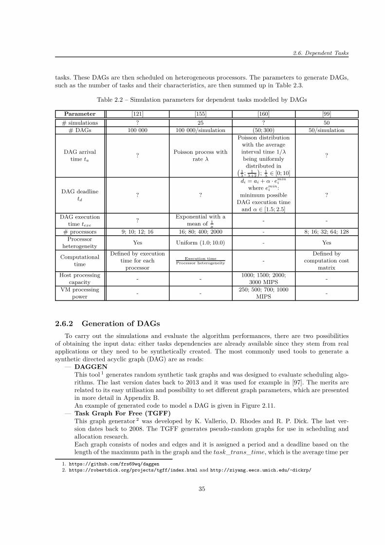
2.6. Dependent Tasks

tasks. These DAGs are then scheduled on heterogeneous processors. The parameters to generate DAGs,such as the number of tasks and their characteristics, are then summed up in Table 2.3.

Table 2.2 – Simulation parameters for dependent tasks modelled by DAGs

Parameter [121] [155] [160] [99]

# simulations ? 25 ? 50

# DAGs 100 000 100 000/simulation (50; 300) 50/simulation

DAG arrivaltime ta

?Poisson process with

rate λ

Poisson distributionwith the averageinterval time 1/λbeing uniformlydistributed in

(

1λ

; 1λ+2

)

; 1λ

∈ [0; 10]

?

DAG deadlinetd

? ?

di = ai + α · emini

where emini :

minimum possibleDAG execution time

and α ∈ [1.5; 2.5]

?

DAG executiontime texe

?Exponential with a

mean of 1µ

- -

# processors 9; 10; 12; 16 16; 80; 400; 2000 - 8; 16; 32; 64; 128

Processorheterogeneity

Yes Uniform (1.0; 10.0) - Yes

Computationaltime

Defined by executiontime for each

processor

Execution timeProcessor heterogeneity -

Defined bycomputation cost

matrix

Host processingcapacity

- -1000; 1500; 2000;

3000 MIPS-

VM processingpower

- -250; 500; 700; 1000

MIPS-

2.6.2 Generation of DAGs

To carry out the simulations and evaluate the algorithm performances, there are two possibilitiesof obtaining the input data: either tasks dependencies are already available since they stem from realapplications or they need to be synthetically created. The most commonly used tools to generate asynthetic directed acyclic graph (DAG) are as reads:

— DAGGENThis tool 1 generates random synthetic task graphs and was designed to evaluate scheduling algo-rithms. The last version dates back to 2013 and it was used for example in [97]. The merits arerelated to its easy utilisation and possibility to set different graph parameters, which are presentedin more detail in Appendix B.An example of generated code to model a DAG is given in Figure 2.11.

— Task Graph For Free (TGFF)This graph generator 2 was developed by K. Vallerio, D. Rhodes and R. P. Dick. The last ver-sion dates back to 2008. The TGFF generates pseudo-random graphs for use in scheduling andallocation research.Each graph consists of nodes and edges and it is assigned a period and a deadline based on thelength of the maximum path in the graph and the task_trans_time, which is the average time per

1. https://github.com/frs69wq/daggen

2. https://robertdick.org/projects/tgff/index.html and http://ziyang.eecs.umich.edu/~dickrp/

35

Chapter 2 – Primary/Backup Approach: Related Work

Table 2.3 – DAG parameters

Parameter [121] [155] [160] [99]

# tasks N 100; 200 20, 40, 60, 80, 100 200500; 1000; 1500;

2000; 2500

# messages U 4N - θ · N ; θ ∈ 2; 7 -

Connectivity -Randomly chosen;

uniform (1%; 100%)(fully connected)

- λ ∈ 0.2; 0.5; 1; 2; 5

# levels - - - ⌈√

Nλ

⌉Width - - - ⌈λ ·

√N⌉

Communicationto computation

cost ratio (CCR)- - - 0.2; 0.5; 1; 2; 5

Communicationtime for each

message

Randomly selectinga sender and a

receiver for eachedge having cost [1;

10]

-

Randomly selectinga sender and a

receiver for eachmessage having size

[10; 100] MB

CCR ·(average taskexecution time)

Task executiontime

Random (5; 50)Uniformly

distributed with amean of texe

N

- Uniform (10; 50)

Task size - -

Uniform(

1 · 105 to 2 · 105)

MI (Millions ofInstructions)

-

Fault detectiontime δ

Randomly chosen;uniform (1; 10)

- - -

Relativedeadline t

Depends on the taskconstraints

Uniformlydistributed with amean of ta + η ·

2·texe

mean processing speed;

η ∈ 0.2; 0.3

According to theDAG deadline

-

// DAG automatically generated by daggen at Fri Jun 8 14:35:27 2018

// ./daggen -n 10 --maxdata 10000 --dot -o DAG_name.dot

digraph G

1 [size="437468061946", alpha="0.04"]

1 -> 6 [size ="679477248"]

2 [size="13268109502", alpha="0.04"]

2 -> 4 [size ="536870912"]

2 -> 5 [size ="536870912"]

2 -> 6 [size ="536870912"]

3 [size="11659573117", alpha="0.18"]

3 -> 4 [size ="411041792"]

4 [size="549755813888", alpha="0.19"]

4 -> 7 [size ="536870912"]

...

Figure 2.11 – Example of DAG generation using DAGGEN

node and edge traversal. A user can set several parameters, such as general ones (e.g. the numberof graphs to generate or the minimum number of tasks per task graph), serial/parallel ones (e.g.the length and the width of series chains, the Boolean to generate a graph with a series-parallel

36

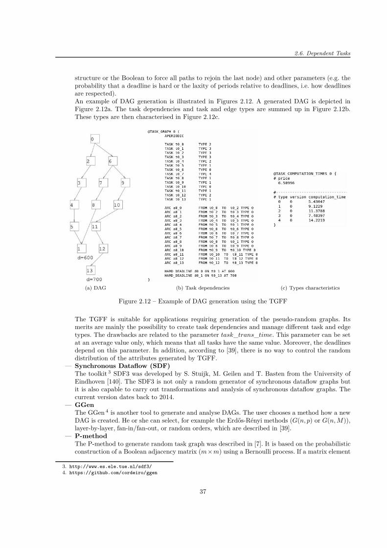
2.6. Dependent Tasks

structure or the Boolean to force all paths to rejoin the last node) and other parameters (e.g. theprobability that a deadline is hard or the laxity of periods relative to deadlines, i.e. how deadlinesare respected).An example of DAG generation is illustrated in Figures 2.12. A generated DAG is depicted inFigure 2.12a. The task dependencies and task and edge types are summed up in Figure 2.12b.These types are then characterised in Figure 2.12c.

(a) DAG (b) Task dependencies (c) Types characteristics

Figure 2.12 – Example of DAG generation using the TGFF

The TGFF is suitable for applications requiring generation of the pseudo-random graphs. Itsmerits are mainly the possibility to create task dependencies and manage different task and edgetypes. The drawbacks are related to the parameter task_trans_time. This parameter can be setat an average value only, which means that all tasks have the same value. Moreover, the deadlinesdepend on this parameter. In addition, according to [39], there is no way to control the randomdistribution of the attributes generated by TGFF.

— Synchronous Dataflow (SDF)The toolkit 3 SDF3 was developed by S. Stuijk, M. Geilen and T. Basten from the University ofEindhoven [140]. The SDF3 is not only a random generator of synchronous dataflow graphs butit is also capable to carry out transformations and analysis of synchronous dataflow graphs. Thecurrent version dates back to 2014.

— GGenThe GGen 4 is another tool to generate and analyse DAGs. The user chooses a method how a newDAG is created. He or she can select, for example the Erdős-Rényi methods (G(n, p) or G(n, M)),layer-by-layer, fan-in/fan-out, or random orders, which are described in [39].

— P-methodThe P-method to generate random task graph was described in [7]. It is based on the probabilisticconstruction of a Boolean adjacency matrix (m×m) using a Bernoulli process. If a matrix element

3. http://www.es.ele.tue.nl/sdf3/

4. https://github.com/cordeiro/ggen

37

Chapter 2 – Primary/Backup Approach: Related Work

aij (where 0 6 i 6 m and 0 6 j 6 m) equals 1, there is a dependency from task ti to task tj .Otherwise, there is no dependency.

If a tool does not provide a graphical visualisation, once a DAG is generated, it can be treated byGraphviz 5. This tool allows one to obtain a graphical representation in different formats, such as imageor PDF files. Graphviz makes use of the DOT language.

2.7 Application of Primary/Backup Approach

The primary/backup approach is a simple method to make system fault tolerant. This section presentsseveral examples, where this approach is successfully used. The use in a system based on dynamic voltageand frequency scaling is covered in Section 2.7.1. Section 2.7.2 then describes how this approach is put intopractice in evolutionary algorithms. The application in virtualised clouds and in satellites are respectivelytreated in Sections 2.7.3 and 2.7.4.

2.7.1 Dynamic Voltage and Frequency Scaling

The paper [67] introduces several algorithms based on the primary/backup approach to scheduleindependent periodic real-time tasks on a multiprocessor system using both the dynamic voltage andfrequency scaling (DVFS) and the dynamic power management (DPM). The aim is to maximize theenergy savings subject to the constraints of (i) tolerating a single permanent fault and (ii) preservingsystem reliability with respect to transient faults (in the absence of permanent faults).

Before describing the algorithms, we briefly summarise the system and task models. The authors con-sider m homogeneous processors with shared memory and they assume that each processor has dynamicvoltage and frequency scaling (DVFS) capability, i.e. it can operate at one of several discrete frequencyand voltage levels.

The system has a set of n independent periodic real-time tasks Γ = T1, ..., Tn. Each task Ti ischaracterised by its worst-case execution time ci and its period pi. The authors consider that the worst-case execution time ci corresponds to the execution time at the maximum available processor frequency.The tasks are assumed to have implicit deadlines: a jth task instance of Ti denoted as Ti,j arrives at time(j − 1) · pi and needs to complete its execution by its deadline at j · pi.

The power consumption of a system with m processors operating respectively at frequencies f1, ..., fm

is expressed as follows:

P (f1, . . . , fm) = Ps +m∑

i=1

~i

(

Pind + Cef · fki

)

(2.2)

where— Ps denotes the system static power,— Pind stands for the frequency-independent active power (assumed to be the same for all processors),— the product Cef · fk

i stands for the frequency-dependent active power depending on the system-dependent constants Cef and k and the frequency fi,

— ~i is Boolean: if a ith processor is active, ~i = 1, otherwise ~i = 0. It means that the processor isswitched to the sleep state through the dynamic power management (DPM) and does not consumeany active power.

Following the model definitions, we describe the algorithms.First, two algorithms based on Standby-Sparing (SS) scheme are introduced: Paired-SS and Generalized-

SS algorithms. In general, the SS scheme schedules offline primary and backup copies separately on theprimary and backup processors. Since the backup copies are normally deallocated once the corresponding

5. https://www.graphviz.org

38

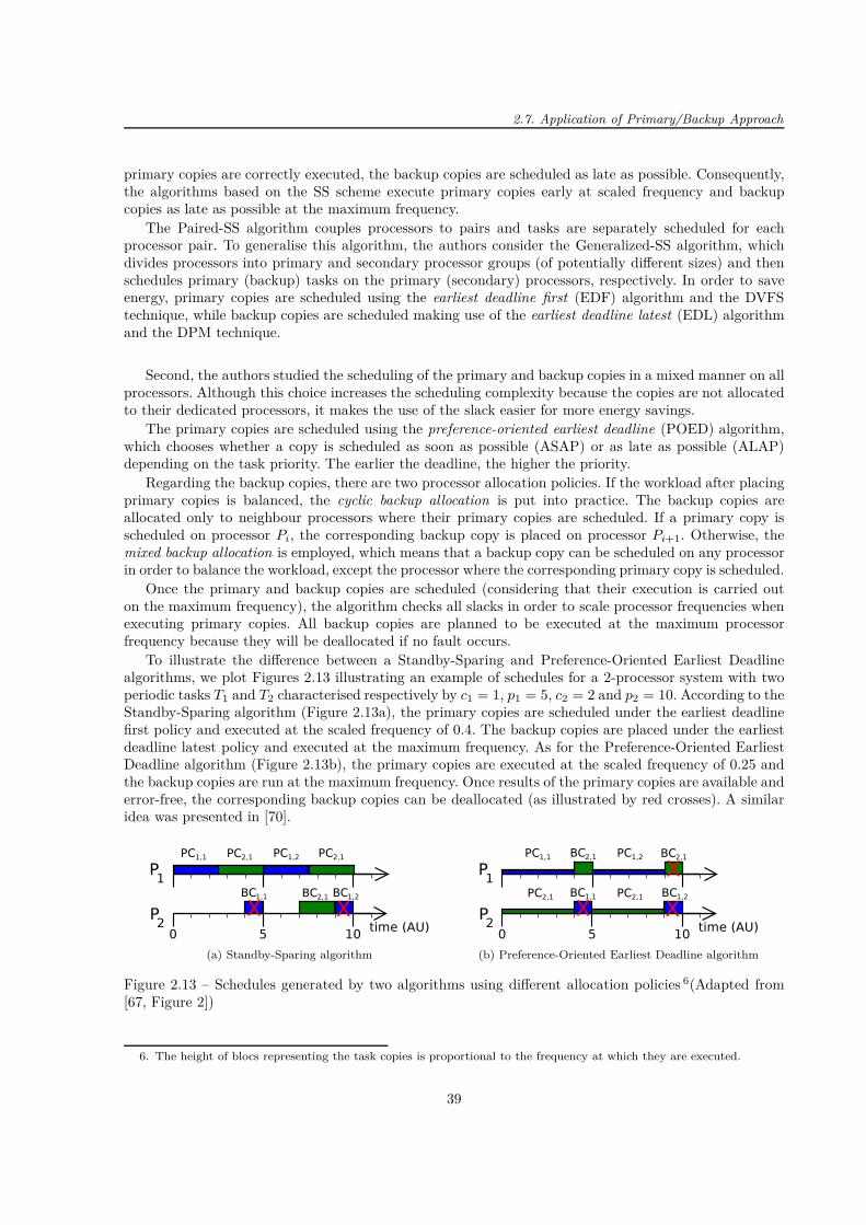
2.7. Application of Primary/Backup Approach

primary copies are correctly executed, the backup copies are scheduled as late as possible. Consequently,the algorithms based on the SS scheme execute primary copies early at scaled frequency and backupcopies as late as possible at the maximum frequency.

The Paired-SS algorithm couples processors to pairs and tasks are separately scheduled for eachprocessor pair. To generalise this algorithm, the authors consider the Generalized-SS algorithm, whichdivides processors into primary and secondary processor groups (of potentially different sizes) and thenschedules primary (backup) tasks on the primary (secondary) processors, respectively. In order to saveenergy, primary copies are scheduled using the earliest deadline first (EDF) algorithm and the DVFStechnique, while backup copies are scheduled making use of the earliest deadline latest (EDL) algorithmand the DPM technique.

Second, the authors studied the scheduling of the primary and backup copies in a mixed manner on allprocessors. Although this choice increases the scheduling complexity because the copies are not allocatedto their dedicated processors, it makes the use of the slack easier for more energy savings.

The primary copies are scheduled using the preference-oriented earliest deadline (POED) algorithm,which chooses whether a copy is scheduled as soon as possible (ASAP) or as late as possible (ALAP)depending on the task priority. The earlier the deadline, the higher the priority.

Regarding the backup copies, there are two processor allocation policies. If the workload after placingprimary copies is balanced, the cyclic backup allocation is put into practice. The backup copies areallocated only to neighbour processors where their primary copies are scheduled. If a primary copy isscheduled on processor Pi, the corresponding backup copy is placed on processor Pi+1. Otherwise, themixed backup allocation is employed, which means that a backup copy can be scheduled on any processorin order to balance the workload, except the processor where the corresponding primary copy is scheduled.

Once the primary and backup copies are scheduled (considering that their execution is carried outon the maximum frequency), the algorithm checks all slacks in order to scale processor frequencies whenexecuting primary copies. All backup copies are planned to be executed at the maximum processorfrequency because they will be deallocated if no fault occurs.

To illustrate the difference between a Standby-Sparing and Preference-Oriented Earliest Deadlinealgorithms, we plot Figures 2.13 illustrating an example of schedules for a 2-processor system with twoperiodic tasks T1 and T2 characterised respectively by c1 = 1, p1 = 5, c2 = 2 and p2 = 10. According to theStandby-Sparing algorithm (Figure 2.13a), the primary copies are scheduled under the earliest deadlinefirst policy and executed at the scaled frequency of 0.4. The backup copies are placed under the earliestdeadline latest policy and executed at the maximum frequency. As for the Preference-Oriented EarliestDeadline algorithm (Figure 2.13b), the primary copies are executed at the scaled frequency of 0.25 andthe backup copies are run at the maximum frequency. Once results of the primary copies are available anderror-free, the corresponding backup copies can be deallocated (as illustrated by red crosses). A similaridea was presented in [70].

(a) Standby-Sparing algorithm (b) Preference-Oriented Earliest Deadline algorithm

Figure 2.13 – Schedules generated by two algorithms using different allocation policies 6(Adapted from[67, Figure 2])

6. The height of blocs representing the task copies is proportional to the frequency at which they are executed.

39

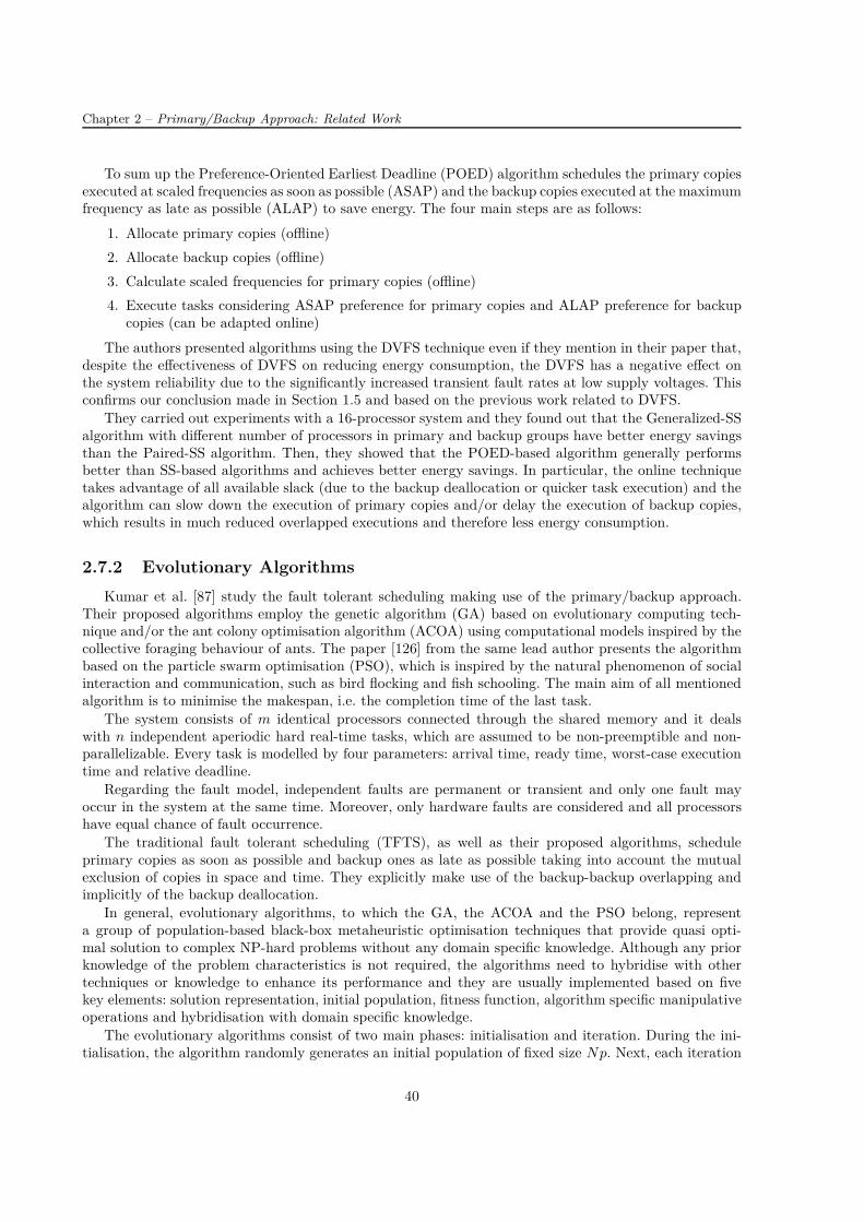
Chapter 2 – Primary/Backup Approach: Related Work

To sum up the Preference-Oriented Earliest Deadline (POED) algorithm schedules the primary copiesexecuted at scaled frequencies as soon as possible (ASAP) and the backup copies executed at the maximumfrequency as late as possible (ALAP) to save energy. The four main steps are as follows:

1. Allocate primary copies (offline)

2. Allocate backup copies (offline)

3. Calculate scaled frequencies for primary copies (offline)

4. Execute tasks considering ASAP preference for primary copies and ALAP preference for backupcopies (can be adapted online)

The authors presented algorithms using the DVFS technique even if they mention in their paper that,despite the effectiveness of DVFS on reducing energy consumption, the DVFS has a negative effect onthe system reliability due to the significantly increased transient fault rates at low supply voltages. Thisconfirms our conclusion made in Section 1.5 and based on the previous work related to DVFS.

They carried out experiments with a 16-processor system and they found out that the Generalized-SSalgorithm with different number of processors in primary and backup groups have better energy savingsthan the Paired-SS algorithm. Then, they showed that the POED-based algorithm generally performsbetter than SS-based algorithms and achieves better energy savings. In particular, the online techniquetakes advantage of all available slack (due to the backup deallocation or quicker task execution) and thealgorithm can slow down the execution of primary copies and/or delay the execution of backup copies,which results in much reduced overlapped executions and therefore less energy consumption.

2.7.2 Evolutionary Algorithms

Kumar et al. [87] study the fault tolerant scheduling making use of the primary/backup approach.Their proposed algorithms employ the genetic algorithm (GA) based on evolutionary computing tech-nique and/or the ant colony optimisation algorithm (ACOA) using computational models inspired by thecollective foraging behaviour of ants. The paper [126] from the same lead author presents the algorithmbased on the particle swarm optimisation (PSO), which is inspired by the natural phenomenon of socialinteraction and communication, such as bird flocking and fish schooling. The main aim of all mentionedalgorithm is to minimise the makespan, i.e. the completion time of the last task.

The system consists of m identical processors connected through the shared memory and it dealswith n independent aperiodic hard real-time tasks, which are assumed to be non-preemptible and non-parallelizable. Every task is modelled by four parameters: arrival time, ready time, worst-case executiontime and relative deadline.

Regarding the fault model, independent faults are permanent or transient and only one fault mayoccur in the system at the same time. Moreover, only hardware faults are considered and all processorshave equal chance of fault occurrence.

The traditional fault tolerant scheduling (TFTS), as well as their proposed algorithms, scheduleprimary copies as soon as possible and backup ones as late as possible taking into account the mutualexclusion of copies in space and time. They explicitly make use of the backup-backup overlapping andimplicitly of the backup deallocation.

In general, evolutionary algorithms, to which the GA, the ACOA and the PSO belong, representa group of population-based black-box metaheuristic optimisation techniques that provide quasi opti-mal solution to complex NP-hard problems without any domain specific knowledge. Although any priorknowledge of the problem characteristics is not required, the algorithms need to hybridise with othertechniques or knowledge to enhance its performance and they are usually implemented based on fivekey elements: solution representation, initial population, fitness function, algorithm specific manipulativeoperations and hybridisation with domain specific knowledge.

The evolutionary algorithms consist of two main phases: initialisation and iteration. During the ini-tialisation, the algorithm randomly generates an initial population of fixed size Np. Next, each iteration

40

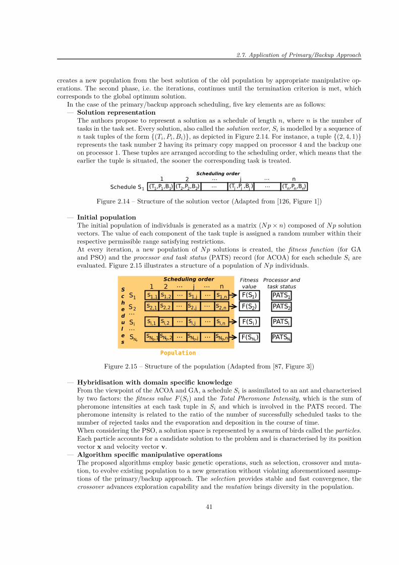
2.7. Application of Primary/Backup Approach

creates a new population from the best solution of the old population by appropriate manipulative op-erations. The second phase, i.e. the iterations, continues until the termination criterion is met, whichcorresponds to the global optimum solution.

In the case of the primary/backup approach scheduling, five key elements are as follows:— Solution representation

The authors propose to represent a solution as a schedule of length n, where n is the number oftasks in the task set. Every solution, also called the solution vector, Si is modelled by a sequence ofn task tuples of the form (Ti, Pi, Bi), as depicted in Figure 2.14. For instance, a tuple (2, 4, 1)represents the task number 2 having its primary copy mapped on processor 4 and the backup oneon processor 1. These tuples are arranged according to the scheduling order, which means that theearlier the tuple is situated, the sooner the corresponding task is treated.

Figure 2.14 – Structure of the solution vector (Adapted from [126, Figure 1])

— Initial populationThe initial population of individuals is generated as a matrix (Np × n) composed of Np solutionvectors. The value of each component of the task tuple is assigned a random number within theirrespective permissible range satisfying restrictions.At every iteration, a new population of Np solutions is created, the fitness function (for GAand PSO) and the processor and task status (PATS) record (for ACOA) for each schedule Si areevaluated. Figure 2.15 illustrates a structure of a population of Np individuals.

Figure 2.15 – Structure of the population (Adapted from [87, Figure 3])

— Hybridisation with domain specific knowledgeFrom the viewpoint of the ACOA and GA, a schedule Si is assimilated to an ant and characterisedby two factors: the fitness value F (Si) and the Total Pheromone Intensity, which is the sum ofpheromone intensities at each task tuple in Si and which is involved in the PATS record. Thepheromone intensity is related to the ratio of the number of successfully scheduled tasks to thenumber of rejected tasks and the evaporation and deposition in the course of time.When considering the PSO, a solution space is represented by a swarm of birds called the particles.Each particle accounts for a candidate solution to the problem and is characterised by its positionvector x and velocity vector v.

— Algorithm specific manipulative operationsThe proposed algorithms employ basic genetic operations, such as selection, crossover and muta-tion, to evolve existing population to a new generation without violating aforementioned assump-tions of the primary/backup approach. The selection provides stable and fast convergence, thecrossover advances exploration capability and the mutation brings diversity in the population.

41

Chapter 2 – Primary/Backup Approach: Related Work

— Fitness functionThe fitness function of solution Si is in general defined as follows:

F (Si) = λ1 · f1 + λ2 · f2 + λ3 · f3

where— λj is a relative weight factor, such as

λ1 + λ2 + λ3 = 1

— fj ∈ [0; 1] is a cost component.In the studied case, the values of λj are experimentally set at 0.7, 0.2 and 0.1 and the costcomponents are associated with the following metrics:— f1= rejection ratio = number of rejected tasks

number of submitted tasks

— f2= processor utilisation deviation ratio = standard deviation in processor utilisationstandard deviation in processor load

— f3= earliest finishing time ratio = earliest finishing time of the last task in Si

maximum absolute deadline among all the tasks in Si

In order to ensure that the cost components data are measured on a neutral scale, all values offitness functions are normalised to [0,1].

The main scheduling steps of the traditional fault tolerant scheduling are as follows:

1. Search for a primary copy slot as soon as possible,

2. Search for a backup copy slot as late as possible,

3. If PC and BC slots exist, commit the task.

Regarding the main scheduling stages for algorithms based on the GA, ACOA or PSO, they are asreads:

1. Setup: if a slot is not empty, remove the first tuple from it,

2. Discard and repeat: check if time constraints are satisfied,

3. Check primary copy slot from the current tuple,

4. Check backup copy slot from the current tuple,

5. If PC and BC slots exist, commit the task.

The simulations being carried out in Matlab, the authors consider 4, 8, 12 and 16 processors. Thealgorithm parameter Np equals 100 all the time and there are 200, 300 or 500 iterations depending on thesize of task set varying 10 to 100. In fact, the population size should be fixed at a reasonably high value(Np = 100) in order to ensure the output stability and the convergence. The TFTS is run without faultsfirst and then with fault injection. The algorithms making use of the GA, ACOA or PSO are simulatedwith fault injection only. One simulation scenario is run 40 times and obtained values are then averaged.

The results are evaluated by means of both the rejection rate and fitness function represented as afunction of the number of executed iterations. The simulations show that the scheduling based on theGA, ACOA or PSO outperform the TFTS. The scheduling based on the GA has faster convergence but isslower when compared to the scheduling with the ACOA. The algorithm using the PSO shows uniformityin processor utilisation in comparison to the TFTS. Moreover, it can be seen that at least 8 iterationsare required to schedule 10 tasks on 4 processors and at least 50 iterations (for GA) or 200 iterations (forACOA) or 250 iterations (for PSO) are necessary to place 100 tasks on 16 processors.

To sum up, the GA, ACOA and PSO present an interesting implementation for the conventional pri-mary/backup approach. On the one hand, as the GA brings the genetic operations, such as the selection,crossover and mutation, and the ACOA fetches the social behaviour, they can avoid that the schedulingalgorithm gets stuck in a local optimum and does not converge. On the other hand, it seems that the useof such techniques is not suitable for systems dealing with the hard real-time tasks because the presentedalgorithm requires many computations even for a small amount of tasks. Actually, the higher the numberof tasks and the lower the number of processors, the slower the convergence.

42

2.7. Application of Primary/Backup Approach

2.7.3 Virtualised Clouds

Zhu et al. [160] make use of the primary-backup approach for the virtualised cloud by taking intoaccount cloud characteristics. First, the cloud uses virtual machines as basic computational instances andallows them to migrate among multiple hosts. Second, the cloud can be scaled up and down dependingon the demand. The authors propose the fault tolerant algorithm, which schedules dependent tasks onthe cloud and which can add or remove resources according to the workload.

Jobs consisting of dependent tasks are modelled by the Directed Acyclic Graph (DAG) denoted byG = T, E, where T = t1, t2, ..., tn is a set of the real-time non-preemptive tasks and E is a set ofthe directed edges that represents dependencies among tasks. Every DAG is defined by arrival time anddeadline. Each task in the DAG is characterised by arrival time, deadline and task size.

The authors consider a virtualised cloud containing a set H = h1, h2, ... of unlimited number ofphysical computing hosts. A host hk ∈ H has its processing capacity pk, which characterises its CPUperformance in Million Instructions Per Second (MIPS), and it can have several virtual machines. Itsvirtual machines represent a set Vk = v1k, v2k, ... and they can have different processing abilities whosesum is at most equal to pk.

Regarding the fault model, the system deals with independent faults, which can be transient orpermanent, and it makes use of a fault-detection mechanism to detect faults. There is at most one hostfailure at the same time.

The authors propose the dynamic fault tolerant scheduling algorithm for real-time scientific workflows,called FASTER that is responsible not only for the scheduling of DAGs but also for the elastic resourceprovisioning. The algorithm processes DAGs, also called workflows, in order of their arrival and it searchesfor a primary copy schedule first and then for a backup copy schedule. The primary and backup copies ofthe same task can be executed in parallel. Furthermore, if one task in the DAG misses its deadline, theDAG is not rejected because its deadline may still be met. If two or more tasks miss their deadlines, theDAG is rejected and all its reserved resources are reclaimed.

The first part of the FASTER schedules the task copies. The primary copies are placed as soon aspossible and the search for free slots starts on hosts having only a few primary copies. The idea is tohave an even distribution of primary copies over all the active hosts in order to increase the possibilityof primary-backup overlapping, which is the same as the primary-backup overloading.

This paper shows that the weak primary copy 7 has more scheduling constraints than the strongprimary copy and the main reason for a primary copy to become weak is that it cannot receive resultsfrom its predecessor before its start time if a fault occurs. To reduce this phenomenon, the algorithm thusschedules the backup copies as soon as possible and starts the search on host already accommodating a lotof backup copies. In fact, if the fault occurrence is rather rare, the primary copies are correctly executedand groups of backup copies are progressively deallocated, which can completely free a host that can bethen switched off. The proposed algorithm does not make use of the backup-backup overlapping.

In order to increase the system schedulability, the authors put into practice the backward time slack,which indicates how long the start time of a task copy can be shifted backward without any impact onthe start time and the status (i.e., strong or weak primary copies) of the subsequent tasks. Besides, theyemploy a reclamation mechanism, which finishes the execution of the backup copy and frees its reservedslot, if the corresponding primary copy is correctly executed.

The second part of the proposed algorithm deals with the cloud elasticity. It means that, when thesystem is charged, the algorithm adds resources, i.e. scales up, to avoid the task rejection and, when theworkload is lower, it turns off resources, i.e. scales down, if they have not been used for a certain amountof time.

There are two possibilities of scaling: the vertical and the horizontal ones. The former one creates orremoves a new virtual machine with the required processing capability and the latter one increases orshrinks the processing capacity of an existing virtual machine.

7. The definitions of "weak" and "strong" primary copies are given in Section 2.6.

43

Chapter 2 – Primary/Backup Approach: Related Work

To measure the algorithm performances, three following metrics are put into practice:— the guarantee ratio (GR) accounting for the percentage of DAGs that are guaranteed to finish

successfully among all submitted DAGs,— the host active time (HAT) standing for the total active time of all hosts in cloud and thus

informing about the system resource consumption,— the ratio of task time over hosts time (RTH), which is the ratio of the sum of the task execution

times to the sum of the host active times and which reflects the system resource utilisation of thesystem.

The results show that when the number of DAGs increases, the guarantee ratio remains the same be-cause the system can dynamically launches new resources. Consequently, the system resource consumptionand utilisation grow. When tasks in the DAG become more dependent, all three studied metrics slightlydecrease because the possibility of executing tasks in parallel declines.

Moreover, when the interarrival time increases, the system becomes less charged, the system resourceconsumption and utilisation remain almost constant because the system can adjust the number of re-sources. Nevertheless, the guarantee ratio increases for the creation of new resources introduces a delaywhich may cause deadline misses of several tasks.

In addition, when the deadline becomes more tight, the guarantee ratio rapidly decreases becausethe task deadlines can be missed due to the time required to launch new resources. For that reason, thesystem resource consumption and utilisation drop as well.

To summarise, the authors present the algorithm that can efficiently schedule dependent tasks atrun-time and dynamically add or remove resources depending on the demand. The algorithm improvesthe system schedulability and resource utilisation. Nonetheless, these merits are at the expense of thealgorithm complexity, which is not studied in this paper. Furthermore, when Naedele [104] carried out theexperiments with independent tasks only, it found out that the results using the slack, which is equivalentto the task backward shifting, may be sometimes worse than the ones without this technique.

2.7.4 Satellites

Zhu et al. [161] present an enhancement based on the primary/backup approach to provide satel-lites with fault tolerance. They propose the Fault-Tolerant Satellite Scheduling (FTSS) algorithm todynamically schedule aperiodic, real-time, independent and non-preemptive tasks. In order to improvethe resource utilisation, the algorithm makes use of the overlapping, which is the same as the overloadingdescribed in [61]. Nevertheless, the technique of backup deallocation is not mentioned in this paper andthus not employed.

The task is modelled by the arrival time, deadline and resolution requirement, which corresponds tothe worst acceptable resolution. Every task has two identical copies: the primary and backup ones. Eachcopy executes on different satellites. Actually, every satellite has one processor and the fault tolerance istherefore ensured by a set of satellites. The satellite is characterised by the duration of task execution, fieldof view angle, slewing pace, start-up time, retention time of shutdown, attitude stability time, maximumslewing angle and the best ground observation resolution. The communication and task dispatching timesare not considered.

The authors then define the available opportunity as a possible slot for a task copy if all time andresolution constraints are fulfilled. An example of the kth available opportunity aoP

ijk for the primarycopy of task Ti on satellite Sj , delimited by the difference between the end PC window weP

ijk and thestart PC window wsP

ijk, is depicted in Figure 2.16. The area captured by satellite Si at the beginningof the available opportunity is coloured in red and purple, whereas the one captured at the end of theavailable opportunity is highlighted in purple and blue. The purple zone illustrates the area where thetask Ti should be in order to be visible during the whole available opportunity.

The fault model considers transient or permanent faults assumed independent. Furthermore, only onefault can occur at the same time and a fault detection mechanism is available to detect it.

44

2.8. Summary

jSatellite S

at the end of aoPijk

Figure 2.16 – Example of the kth available opportunity aoPijk for the primary copy of task Ti on satellite

Sj (Adapted from [161, Figure 1])

The main objective of the presented algorithm is to maximise the guarantee ratio and then to minimizethe observation resolutions of all accepted tasks under time constraints.

The algorithm schedules the primary copies as soon as possible and the backup ones as late as possibleafter scouring for available opportunities on all processors to find the best solution in a sense of the mainobjectives. To enhance the algorithm performances, the backup-backup overlapping, described in [61], andthe primary-backup overlapping, presented in [6], are implemented. Considering that a task Ti arrivesearlier than a task Tj , the authors point out that the latter technique cannot be used for P Cj and BCi

if the start time of P Bj is earlier than the one of BCi because P Cj cannot be interrupted during itsexecution.

In addition, taking into account that a scene can be seen by several satellites at the same time (butwith different properties, such as the resolution or angle), it is possible to merge some tasks together inorder to improve the schedulability. Consequently, when an image is the same for two different primarycopies, these copies can jointly merge if several merging constraints on the existence and size of overlappedtime window, the observation angle and the resolution are met.

The simulation parameters are set at the following values: the latitude between -30°and 60°, thelongitude between 0°and 150°, the number of tasks in range from 200 to 1 200 and the number ofsatellites at 10. The interarrival time is uniformly distributed. To assess the algorithm performances, theauthors evaluate the guarantee ratio and the observation resolution accounting for the average observationresolution of accepted tasks.

Their experiments compare the proposed algorithm with the basic one (no merging and no overlap-ping), the one with merging only and the one with overlapping only. It can be observed that the use of thetask merging and overlapping together generally achieves better results, i.e. higher guarantee ratio andlower observation resolution. Besides, the more tasks, the higher observation resolution and the worse theguarantee ratio due to higher system workload. In general, the longer the interarrival time, the higherthe guarantee ratio because they are less arriving tasks. Nevertheless, when the interarrival time is tooshort, the values of the guarantee ratio are comparable with the ones when the interarrival time is highfor many tasks can be merged. Moreover, it is shown that the tighter the task deadline, the lower theguarantee ratio.

2.8 Summary

This chapter summed up the work related to the primary/backup approach. It covers the advent ofthis approach and already proposed enhancing techniques: the primary slack, decision deadline, activeapproach, replication cost with boundary schedules and primary-backup overloading. It also showedseveral applications of this approach, such as its use in the dynamic voltage and frequency scaling,evolutionary algorithms, virtualised clouds, or satellites.

45

Chapter 2 – Primary/Backup Approach: Related Work

While this chapter dealt with already publish work, the next chapter presents our research on theprimary/backup approach.

46

Chapter 3

PRIMARY/BACKUP APPROACH: OUR

ANALYSIS

The preceding chapter is a compilation based on already published sources related to the prima-ry/backup approach. The first part of this chapter is devoted to independent tasks, whereas the secondone treats dependent tasks.

This chapter presents our task, system and fault models. Following the mathematical problem formu-lation, different processor allocation policies and scheduling search techniques are compared. Next, threeproposed enhancing techniques are introduced: (i) the method of restricted scheduling windows withinwhich the primary and backup copies can be scheduled, (ii) the method of limitation on the number ofcomparisons, accounting for the algorithm run-time, when scheduling a task on a system, and (iii) themethod of several scheduling attempts. Finally, the experimental framework is described and results areanalysed in fault-free and harsh environments.

Regarding the dependent tasks, this chapter presents how we deal with directed acyclic graphics andwhich aforementioned techniques are put into practice. The results are then described and discussed.

3.1 Independent Tasks

This section covers independent tasks, i.e. there exist no task dependencies.

3.1.1 Assumptions and Scheduling Model

A hard real-time system is composed of P interconnected identical processors sharing the same mem-ory. Although the system with only homogeneous processors is considered, it would be possible to extendthis model to a system with heterogeneous processors, such as in [155] by defining different processorspeeds or different computation times. While a centralised memory is put into practice, a distributedmemory could be used as well. The principle of the studied method would remain the same but it wouldnecessitate to take delays of data transfers into account.

The aperiodic tasks are online scheduled on such a system without preemption. We assume the exis-tence of fault detection mechanism and that it can promptly inform if a permanent and/or transient faultoccurs. A fault can be detected for example by acceptance tests, such as timing, coding, reasonablenessor structural checks [49].

We consider that only one processor failure can occur at any instant of time and that the scheduleris enough robust, e.g. using a spare scheduler if necessary. Current processors have a failure rate of1/120 h−1 [47] and, although the reliability of P -processor system is lower, our assumption holds. In fact,the authors in [72] proved that a system consisting of identical processors has its reliability (measured bymeans of the mean time between faults (MTBF)) equal to the processor MTBF divided by the numberof processors. (For more details see Section 1.3.4.)

Using Graham’s classification [66] described in Section 1.1, the analysed problem is defined as

P ; m | n = k; online rj ; dj = d; pj = p | (check the feasibility of schedule)

47

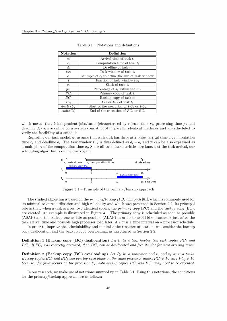
Chapter 3 – Primary/Backup Approach: Our Analysis

Table 3.1 – Notations and definitions

Notation Definition

ai Arrival time of task ti

ci Computation time of task ti

di Deadline of task ti

twi Task window of task ti

α Multiple of ci to define the size of task window

f Fraction of task window twi

si Slack of task ti

psi Percentage of si within the twi

P Ci Primary copy of task ti

BCi Backup copy of task ti

xCi P C or BC of task ti

start(xCi) Start of the execution of P Ci or BCi

end(xCi) End of the execution of P Ci or BCi

which means that k independent jobs/tasks (characterised by release time rj , processing time pj anddeadline dj) arrive online on a system consisting of m parallel identical machines and are scheduled toverify the feasibility of a schedule.

Regarding our task model, we assume that each task has three attributes: arrival time ai, computationtime ci and deadline di. The task window twi is thus defined as di − ai and it can be also expressed asa multiple α of the computation time ci. Since all task characteristics are known at the task arrival, ourscheduling algorithm is online clairvoyant.

Figure 3.1 – Principle of the primary/backup approach

The studied algorithm is based on the primary/backup (PB) approach [61], which is commonly used forits minimal resource utilisation and high reliability and which was presented in Section 2.2. Its principalrule is that, when a task arrives, two identical copies, the primary copy (PC) and the backup copy (BC),are created. An example is illustrated in Figure 3.1. The primary copy is scheduled as soon as possible(ASAP) and the backup one as late as possible (ALAP) in order to avoid idle processors just after thetask arrival time and possible high processor load later. A slot is a time interval on a processor schedule.

In order to improve the schedulability and minimise the resource utilisation, we consider the backupcopy deallocation and the backup copy overloading, as introduced in Section 2.2.

Definition 1 (Backup copy (BC) deallocation) Let ti be a task having two task copies P Ci andBCi. If P Ci was correctly executed, then BCi can be deallocated and free its slot for new arriving tasks.

Definition 2 (Backup copy (BC) overloading) Let Px be a processor and ti and tj be two tasks.Backup copies BCi and BCj can overlap each other on the same processor unless P Ci ∈ Px and P Cj ∈ Px

because, if a fault occurs on the processor Px, both backup copies BCi and BCj may need to be executed.

In our research, we make use of notations summed up in Table 3.1. Using this notations, the conditionsfor the primary/backup approach are as follows:

48

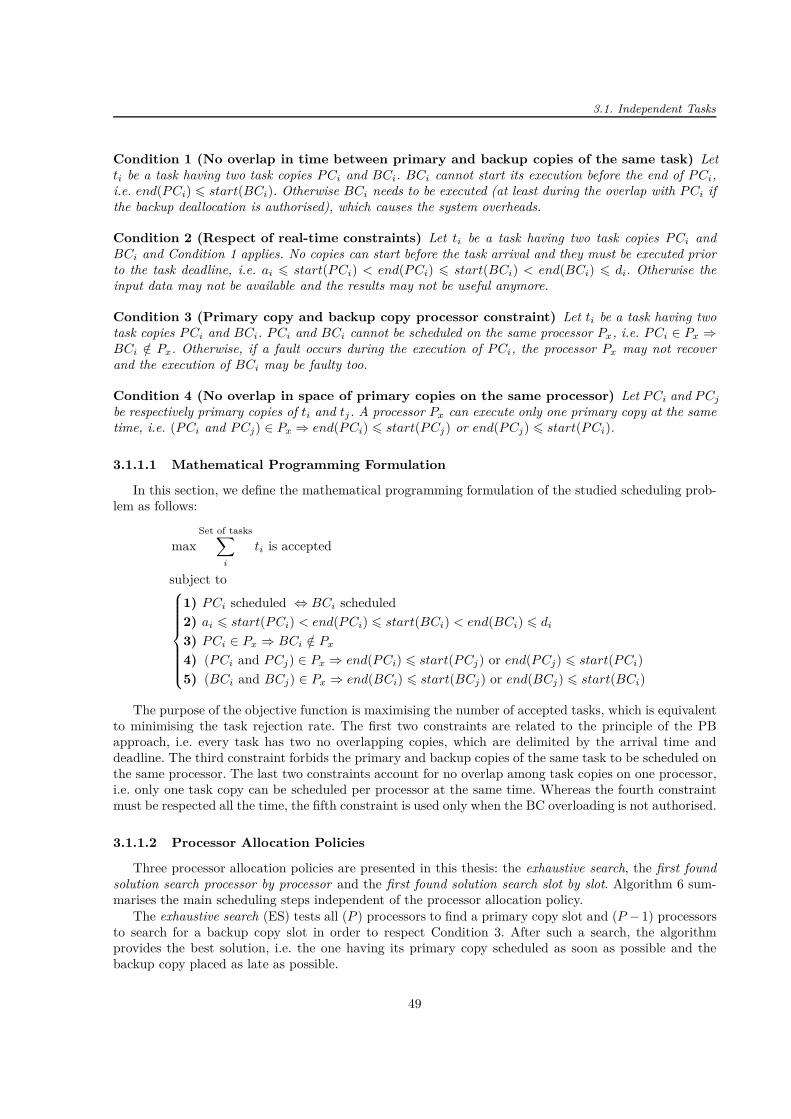
3.1. Independent Tasks

Condition 1 (No overlap in time between primary and backup copies of the same task) Letti be a task having two task copies P Ci and BCi. BCi cannot start its execution before the end of P Ci,i.e. end(P Ci) 6 start(BCi). Otherwise BCi needs to be executed (at least during the overlap with P Ci ifthe backup deallocation is authorised), which causes the system overheads.

Condition 2 (Respect of real-time constraints) Let ti be a task having two task copies P Ci andBCi and Condition 1 applies. No copies can start before the task arrival and they must be executed priorto the task deadline, i.e. ai 6 start(P Ci) < end(P Ci) 6 start(BCi) < end(BCi) 6 di. Otherwise theinput data may not be available and the results may not be useful anymore.

Condition 3 (Primary copy and backup copy processor constraint) Let ti be a task having twotask copies P Ci and BCi. P Ci and BCi cannot be scheduled on the same processor Px, i.e. P Ci ∈ Px ⇒BCi /∈ Px. Otherwise, if a fault occurs during the execution of P Ci, the processor Px may not recoverand the execution of BCi may be faulty too.

Condition 4 (No overlap in space of primary copies on the same processor) Let P Ci and P Cj

be respectively primary copies of ti and tj. A processor Px can execute only one primary copy at the sametime, i.e. (P Ci and P Cj) ∈ Px ⇒ end(P Ci) 6 start(P Cj) or end(P Cj) 6 start(P Ci).

3.1.1.1 Mathematical Programming Formulation

In this section, we define the mathematical programming formulation of the studied scheduling prob-lem as follows:

maxSet of tasks∑

i

ti is accepted

subject to

1) P Ci scheduled ⇔ BCi scheduled2) ai 6 start(P Ci) < end(P Ci) 6 start(BCi) < end(BCi) 6 di

3) P Ci ∈ Px ⇒ BCi /∈ Px

4) (P Ci and P Cj) ∈ Px ⇒ end(P Ci) 6 start(P Cj) or end(P Cj) 6 start(P Ci)5) (BCi and BCj) ∈ Px ⇒ end(BCi) 6 start(BCj) or end(BCj) 6 start(BCi)

The purpose of the objective function is maximising the number of accepted tasks, which is equivalentto minimising the task rejection rate. The first two constraints are related to the principle of the PBapproach, i.e. every task has two no overlapping copies, which are delimited by the arrival time anddeadline. The third constraint forbids the primary and backup copies of the same task to be scheduled onthe same processor. The last two constraints account for no overlap among task copies on one processor,i.e. only one task copy can be scheduled per processor at the same time. Whereas the fourth constraintmust be respected all the time, the fifth constraint is used only when the BC overloading is not authorised.

3.1.1.2 Processor Allocation Policies

Three processor allocation policies are presented in this thesis: the exhaustive search, the first foundsolution search processor by processor and the first found solution search slot by slot. Algorithm 6 sum-marises the main scheduling steps independent of the processor allocation policy.

The exhaustive search (ES) tests all (P ) processors to find a primary copy slot and (P − 1) processorsto search for a backup copy slot in order to respect Condition 3. After such a search, the algorithmprovides the best solution, i.e. the one having its primary copy scheduled as soon as possible and thebackup copy placed as late as possible.

49

Chapter 3 – Primary/Backup Approach: Our Analysis

Algorithm 6 Primary/backup schedulingInput: Task ti, Mapping and scheduling MS of already scheduled tasksOutput: Updated mapping and scheduling MS

1: if new task ti arrives then2: Map and schedule P Ci

3: Map and schedule BCi

4: if PC and BC slots exist then5: Commit the task ti

6: else7: Reject the task ti

The second and third processor allocation policies are mainly meant for real-time systems, which maynot have time to search for a solution on all processors, assess all possibilities and then opt for the bestone. The idea is to find a solution as quickly as possible and not necessarily the best one. Naedele [103]presented the sequential search, which we call the first found solution search - processor by processor(FFSS PbP). The algorithm goes through processors, one by one, until it finds a slot large enough toplace a copy or until it scours all processors, as it is depicted in Figure 3.2a. There is no restriction onscheduling, which means that a primary copy can be scheduled rather late within the task window. Thisdecreases the chance to place the corresponding backup copy within the remaining scheduling windowand subsequently increases the task rejection rate.

(a) Processor by Processor (PbP) (b) Slot by Slot (SbS)

Figure 3.2 – Principle of the First Found Solution Search (FFSS)

In order to improve the previous method and favour placing primary copies as soon as possible, wepropose the processor allocation policy called the first found solution search - slot by slot (FFSS SbS).It starts to check the first free slot on each processor and then, if solution is not found, it continues withnext slots (second, third, ...) until a solution is obtained or it tests all free slots on all processors. Theprinciple of this policy is illustrated in Figure 3.2b.

The selection of the processor on which the search for a slot starts plays an important role in the systemschedulability and workload distribution among processors [103]. Therefore, to avoid a non-uniformityof the processor load for both PbP and SbS, the FFSS for a primary copy slot starts on the processorfollowing the processor on which the primary copy of the previous task was successfully scheduled. Thesearch then continues in increasing order of the processors until a slot is found or all processors arescoured [103]. If a primary copy slot of a new task is found on processor Px, a search for a backup copyslot is carried out. It starts on processor Px−1 and it proceeds in decreasing order of the processors till aslot is found or no more processor is available.

3.1.1.3 Scheduling Search Techniques

There exist several techniques to search for schedules of primary and backup copies. In this manuscript,we analyse two of them: one presented by Ghosh et al. [61], which we call the free slot search technique(FSST), and one introduced by Zheng et al. [155] and named the boundary schedule search technique(BSST). Since the latter technique is not compatible with one of our objectives, i.e. to reduce the algorithm

50

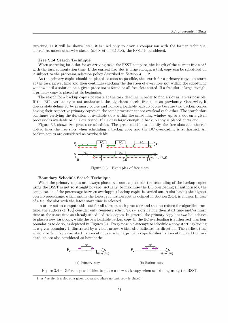
3.1. Independent Tasks

run-time, as it will be shown later, it is used only to draw a comparison with the former technique.Therefore, unless otherwise stated (see Section 3.1.3.8), the FSST is considered.

Free Slot Search TechniqueWhen searching for a slot for an arriving task, the FSST compares the length of the current free slot 1

with the task computation time. If the current free slot is large enough, a task copy can be scheduled onit subject to the processor selection policy described in Section 3.1.1.2.

As the primary copies should be placed as soon as possible, the search for a primary copy slot startsat the task arrival time and then continues checking the duration of every free slot within the schedulingwindow until a solution on a given processor is found or all free slots tested. If a free slot is large enough,a primary copy is placed at its beginning.

The search for a backup copy slot starts at the task deadline in order to find a slot as late as possible.If the BC overloading is not authorised, the algorithm checks free slots as previously. Otherwise, itchecks slots delimited by primary copies and non-overloadable backup copies because two backup copieshaving their respective primary copies on the same processor cannot overload each other. The search thuscontinues verifying the duration of available slots within the scheduling window up to a slot on a givenprocessor is available or all slots tested. If a slot is large enough, a backup copy is placed at its end.

Figure 3.3 shows two processor schedules. The green solid lines identify the free slots and the reddotted lines the free slots when scheduling a backup copy and the BC overloading is authorised. Allbackup copies are considered as overloadable.

Figure 3.3 – Examples of free slots

Boundary Schedule Search TechniqueWhile the primary copies are always placed as soon as possible, the scheduling of the backup copies

using the BSST is not so straightforward. Actually, to maximise the BC overloading (if authorised), thecomputation of the percentage between overlapping backup copies is carried out. A slot having the highestoverlap percentage, which means the lowest replication cost as defined in Section 2.4.4, is chosen. In caseof a tie, the slot with the latest start time is selected.

In order not to compute this cost for all slots on each processor and thus to reduce the algorithm run-time, the authors of [155] consider only boundary schedules, i.e. slots having their start time and/or finishtime at the same time as already scheduled task copies. In general, the primary copy has two boundariesto place a new task copy, while the overloadable backup copy (if the BC overloading is authorised) has fourboundaries to do so, as depicted in Figures 3.4. Every possible attempt to schedule a copy starting/endingat a given boundary is illustrated by a violet arrow, which also indicates its direction. The earliest timewhen a backup copy can start its execution, i.e. when a primary copy finishes its execution, and the taskdeadline are also considered as boundaries.

(a) Primary copy (b) Backup copy

Figure 3.4 – Different possibilities to place a new task copy when scheduling using the BSST

1. A free slot is a slot on a given processor, where no task copy is placed.

51

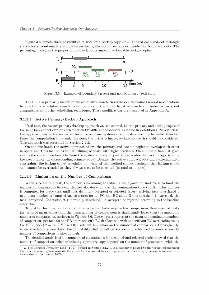
Chapter 3 – Primary/Backup Approach: Our Analysis

Figure 3.5 depicts three possibilities of slots for a backup copy BCv. The red dash-and-dot rectanglestands for a non-boundary slot, whereas two green dotted rectangles denote the boundary slots. Thepercentage indicates the proportion of overlapping among overloadable backup copies.

Figure 3.5 – Example of boundary (green) and non-boundary (red) slots

The BSST is primarily meant for the exhaustive search. Nevertheless, we realised several modificationsto adapt this scheduling search technique also to the non-exhaustive searches in order to carry outcomparisons with other scheduling techniques. These modifications are presented in Appendix A.

3.1.1.4 Active Primary/Backup Approach

Until now, the passive primary/backup approach was considered, i.e. the primary and backup copies ofthe same task cannot overlap each other on two different processors, as stated in Condition 1. Nevertheless,this approach may be too restrictive for some real-time systems since the deadline may be earlier than twotimes the computation time and, therefore, the active primary/backup approach should be considered.This approach was presented in Section 2.4.3.

On the one hand, the active approach allows the primary and backup copies to overlap each otherin space and thus facilitates the scheduling of tasks with tight deadlines. On the other hand, it givesrise to the system overheads because the system entirely or partially executes the backup copy (duringthe execution of the corresponding primary copy). Besides, the active approach adds more schedulabilityconstraints: the backup copies scheduled by means of this method cannot overload other backup copiesand cannot be overloaded as they always need to be executed (in total or in part).

3.1.1.5 Limitation on the Number of Comparisons

When scheduling a task, the simplest idea aiming at reducing the algorithm run-time is to limit thenumber of comparisons between the free slot duration and the computation time ci [103]. This numberis computed for every task until it is definitely accepted or rejected. Every arriving task is assigned amaximum number of comparisons to search for its PC and BC slots. If this threshold is exceeded, thetask is rejected. Otherwise, it is normally scheduled, i.e. accepted or rejected according to the baselinealgorithm.

To justify this idea, we found out that accepted tasks require less comparisons than rejected tasks(in terms of mean values) and the mean number of comparisons is significantly lower than the maximumnumber of comparisons, as shown in Figures 3.6. These figures represent the mean and maximum numbersof comparisons per task for the PB approach with BC deallocation with and without BC overloading usingthe FFSS SbS (P = 14, T P L = 1.0) 2 without limitation on the number of comparisons. Consequently,when scheduling a new task, the probability that it will be successfully scheduled is lower when thenumber of comparisons is already high.

The detailed analysis of the numbers of comparisons for accepted and rejected copies showed that thenumber of comparisons when scheduling a primary copy depends on the number of processors, while the

2. The Targeted Processor Load (TPL), defined in Section 3.1.2.1, is a parameter related to the theoretical processorload when generating task arrivals. If T P L = 1.0, the arrival times are generated so that every processor is considered tobe working all the time at 100%.

52

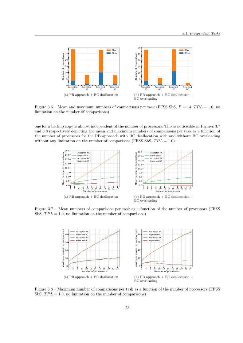
3.1. Independent Tasks

Accepted PC

Accepted BC

Rejected PC

Rejected BC

0

5

10

15

20

25

Numbe

r of c

ompa

rison

s

MaxMean

(a) PB approach + BC deallocation

Accepted PC

Accepted BC

Rejected PC

Rejected BC

0

5

10

15

20

25

30

Numbe

r of c

ompa

rison

s

MaxMean

(b) PB approach + BC deallocation +BC overloading

Figure 3.6 – Mean and maximum numbers of comparisons per task (FFSS SbS, P = 14, T P L = 1.0, nolimitation on the number of comparisons)

one for a backup copy is almost independent of the number of processors. This is noticeable in Figures 3.7and 3.8 respectively depicting the mean and maximum numbers of comparisons per task as a function ofthe number of processors for the PB approach with BC deallocation with and without BC overloadingwithout any limitation on the number of comparisons (FFSS SbS, T P L = 1.0).

2 4 6 8 10 12 14 16 18 20 22 24Number of processors

0.0

2.5

5.0

7.5

10.0

12.5

15.0

17.5

20.0

Mean number o

f com

parisons Accepted PC

Rejected PCAccepted BCRejected BC

(a) PB approach + BC deallocation

2 4 6 8 10 12 14 16 18 20 22 24Number of processors

0.0

2.5

5.0

7.5

10.0

12.5

15.0

17.5

20.0

Mean number o

f com

parisons Accepted PC

Rejected PCAccepted BCRejected BC

(b) PB approach + BC deallocation +BC overloading

Figure 3.7 – Mean numbers of comparisons per task as a function of the number of processors (FFSSSbS, T P L = 1.0, no limitation on the number of comparisons)

2 4 6 8 10 12 14 16 18 20 22 24Number of processors

0

10

20

30

40

Max

imum

num

ber o

f com

paris

ons

Accepted PCRejected PCAccepted BCRejected BC

(a) PB approach + BC deallocation

2 4 6 8 10 12 14 16 18 20 22 24Number of processors

0

10

20

30

40

Max

imum

num

ber o

f com

paris

ons

Accepted PCRejected PCAccepted BCRejected BC

(b) PB approach + BC deallocation +BC overloading

Figure 3.8 – Maximum number of comparisons per task as a function of the number of processors (FFSSSbS, T P L = 1.0, no limitation on the number of comparisons)

53

Chapter 3 – Primary/Backup Approach: Our Analysis

Regarding the backup copies, the mean number of comparisons is between 1 and 2 and the maximumnumber of comparisons can exceed 10. In our simulations, we set the BC threshold at 5 to avoid thata task is often rejected due to missing free slot for a backup copy. Therefore, we define the theoreticalmaximum value of the run-time rtlimit as reads:

rtlimit = rtlimit(P C) + rtlimit(BC) = γ · P + 5 (3.1)

where γ is the limitation coefficient for primary copies expressed in our simulation framework as a functionof the number of processors.

To illustrate Equation 3.1, Figures 3.9 plot the theoretical limitation on the maximum number ofcomparisons per task for the PB approach with BC deallocation with and without BC overloading as afunction of the number of processors (FFSS SbS, T P L = 1.0). As a baseline, represented by the bluecurve, we make use of our experimental results when a limitation is not considered.

2 4 6 8 10 12 14 16 18 20 22 24Number of processors

10

20

30

40

Max

imum

num

ber o

f com

paris

ons

(a) PB approach + BC deallocation

2 4 6 8 10 12 14 16 18 20 22 24Number of processors

51015202530354045

Maxim

um num

ber o

f com

paris

ons

(b) PB approach + BC deallocation +BC overloading

Figure 3.9 – Theoretical limitation on the maximum number of comparisons per task as a function of thenumber of processors (FFSS SbS, T P L = 1.0)

3.1.1.6 Restricted Scheduling Windows

The second method to reduce the algorithm run-time when scheduling a task is called the restrictedscheduling windows. Before giving a definition, we examine positions of the primary and backup copieswithin the task window. As an example, we consider a 14-processor system (with T P L = 1.0) withoutusing the method of restricted scheduling windows. In such a case, the numbers of occurrences, wherethe primary and backup copies respectively start or finish their execution, as a function of the positionin the task window are depicted in Figures 3.10. The results are shown for the PB approach with BCdeallocation but they are almost the same for the PB approach with BC deallocation and with BCoverloading.

It can be seen that, although the algorithm tries to schedule the primary copies as soon as possible,a non-negligible amount of them starts later than at the task arrival time, as illustrated in Figure 3.10a.Regarding the backup copies, the majority of them finishes at the task deadline thanks to the BC deal-location, as depicted in Figure 3.10b.

Therefore, the aim of the method of restricted scheduling windows is threefold:

1. to avoid the mutual scheduling interference between primary and backup copies of the same task,

2. to reduce the run-time (measured by means of the number of comparisons carried out beforedefinitely accepting or rejecting a task),

3. to favour placing the primary copies as soon as possible and the backup ones as late as possible,which increases the schedulability if the BC deallocation is enabled.

54

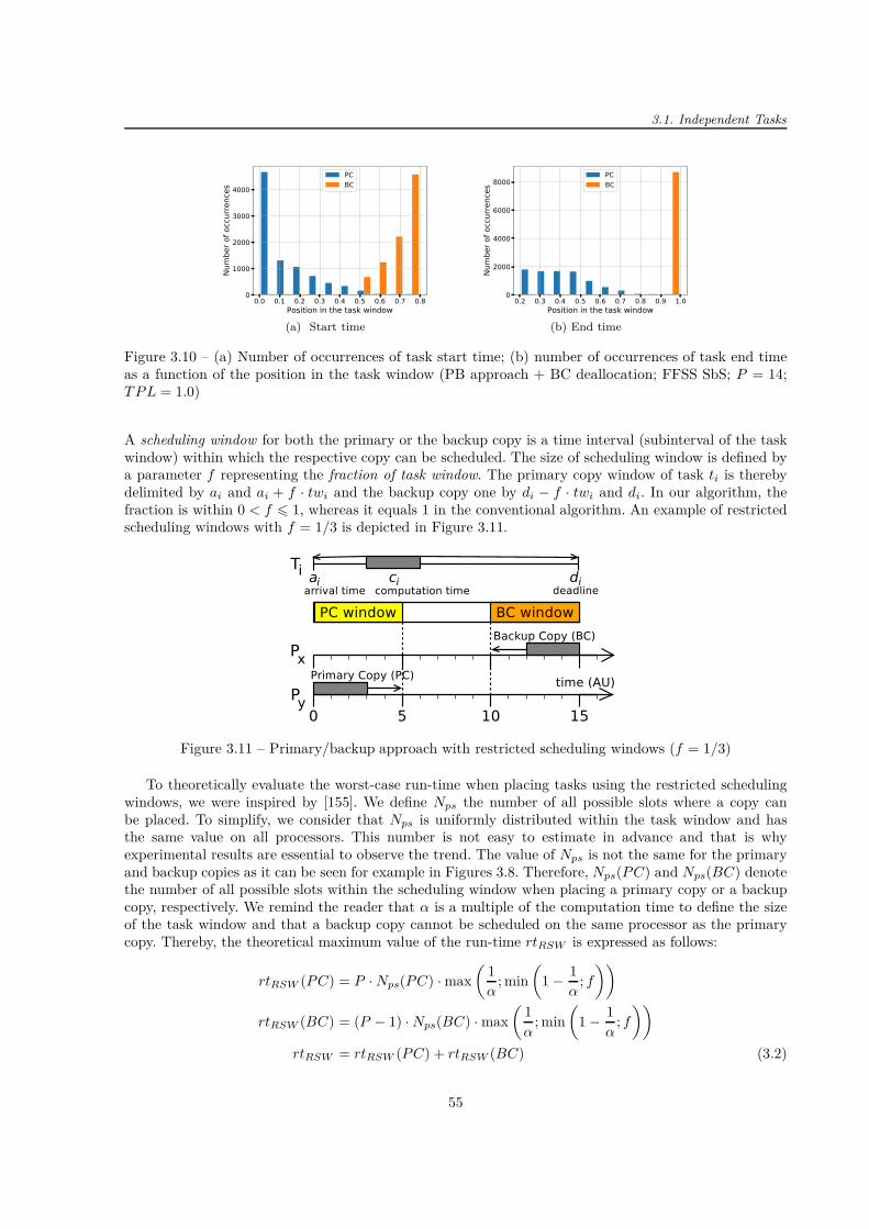
3.1. Independent Tasks

0.0 0.1 0.2 0.3 0.4 0.5 0.6 0.7 0.8Position in the task window

0

1000

2000

3000

4000

Numbe

r of o

ccurrences

PCBC

(a) Start time

0.2 0.3 0.4 0.5 0.6 0.7 0.8 0.9 1.0Position in the task window

0

2000

4000

6000

8000

Number of occurrences

PCBC

(b) End time

Figure 3.10 – (a) Number of occurrences of task start time; (b) number of occurrences of task end timeas a function of the position in the task window (PB approach + BC deallocation; FFSS SbS; P = 14;T P L = 1.0)

A scheduling window for both the primary or the backup copy is a time interval (subinterval of the taskwindow) within which the respective copy can be scheduled. The size of scheduling window is defined bya parameter f representing the fraction of task window. The primary copy window of task ti is therebydelimited by ai and ai + f · twi and the backup copy one by di − f · twi and di. In our algorithm, thefraction is within 0 < f 6 1, whereas it equals 1 in the conventional algorithm. An example of restrictedscheduling windows with f = 1/3 is depicted in Figure 3.11.

Figure 3.11 – Primary/backup approach with restricted scheduling windows (f = 1/3)

To theoretically evaluate the worst-case run-time when placing tasks using the restricted schedulingwindows, we were inspired by [155]. We define Nps the number of all possible slots where a copy canbe placed. To simplify, we consider that Nps is uniformly distributed within the task window and hasthe same value on all processors. This number is not easy to estimate in advance and that is whyexperimental results are essential to observe the trend. The value of Nps is not the same for the primaryand backup copies as it can be seen for example in Figures 3.8. Therefore, Nps(P C) and Nps(BC) denotethe number of all possible slots within the scheduling window when placing a primary copy or a backupcopy, respectively. We remind the reader that α is a multiple of the computation time to define the sizeof the task window and that a backup copy cannot be scheduled on the same processor as the primarycopy. Thereby, the theoretical maximum value of the run-time rtRSW is expressed as follows:

rtRSW (P C) = P · Nps(P C) · max(

1α

; min(

1 − 1α

; f

))

rtRSW (BC) = (P − 1) · Nps(BC) · max(

1α

; min(

1 − 1α

; f

))

rtRSW = rtRSW (P C) + rtRSW (BC) (3.2)

55

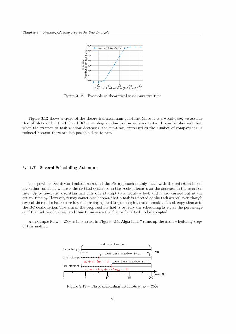
Chapter 3 – Primary/Backup Approach: Our Analysis

0.2 0.4 0.6 0.8 1.0Fraction of task window (P=14, α=3.5)

25

30

35

40

45

50

55

60

Run-

time

(Num

ber o

f com

paris

ons)

Nps(PC)=4; Nps(BC)=2

Figure 3.12 – Example of theoretical maximum run-time

Figure 3.12 shows a trend of the theoretical maximum run-time. Since it is a worst-case, we assumethat all slots within the PC and BC scheduling window are respectively tested. It can be observed that,when the fraction of task window decreases, the run-time, expressed as the number of comparisons, isreduced because there are less possible slots to test.

3.1.1.7 Several Scheduling Attempts

The previous two devised enhancements of the PB approach mainly dealt with the reduction in thealgorithm run-time, whereas the method described in this section focuses on the decrease in the rejectionrate. Up to now, the algorithm had only one attempt to schedule a task and it was carried out at thearrival time ai. However, it may sometimes happen that a task is rejected at the task arrival even thoughseveral time units later there is a slot freeing up and large enough to accommodate a task copy thanks tothe BC deallocation. The aim of the proposed method is to retry the scheduling later, at the percentageω of the task window twi, and thus to increase the chance for a task to be accepted.

An example for ω = 25% is illustrated in Figure 3.13. Algorithm 7 sums up the main scheduling stepsof this method.

ai = 4 di = 20

task window twi

new task window tw2,i

new task window tw3,iai + ω · twi = 8

ai + ω · twi + ω · tw2,i = 11

Figure 3.13 – Three scheduling attempts at ω = 25%

56

3.1. Independent Tasks

Algorithm 7 Algorithm using the method of several scheduling attemptsInput: Task ti, Mapping and scheduling MS of already scheduled tasksOutput: Updated mapping and scheduling MS

1: if new task ti arrives then2: Search for PC and BC slots for the first time3: if PC and BC slots exist then4: Commit the task ti

5: else6: while task not scheduled and new attempt authorised do7: Compute the time of new attempt to schedule the task8: Search for PC and BC slots9: if PC and BC slots exist then

10: Commit the task ti

11: if task not scheduled and new attempt not authorised then12: Reject the task ti

To evaluate the efficiency of this method, we define the percentage of slack within the task window psi

of task ti as follows:

psi =si

twi=

twi − 2 · ci

twi(3.3)

where si denotes the slack, i.e. the remaining time within the task window twi after subtracting twicethe computation time ci necessary for the primary and backup copies to be executed. The higher thepercentage psi, the higher the chance to schedule a task later than at its arrival time. Nonetheless, thehigher the number of scheduling attempts for one task, the lower the probability for new schedulingattempts to be successful because there is less and less slack.

3.1.2 Experimental Framework

In this section, we describe our simulation scenario and define metrics used to evaluate our algorithms.

3.1.2.1 Simulation Scenario

Table 3.2 sums up the simulation parameters. For each simulation scenario, 100 simulations of 10 000tasks were treated and the obtained values were averaged. Unless the simulations with fault injections arecarried out (see Section 3.1.3.13), we consider that no fault occurs during our simulations. Therefore, ifthe BC deallocation is put into practice, all backup copies are deallocated when their respective primarycopies finish.

The arrival times are generated using the Poisson distribution with parameter λ expressed as follows:

λ =average c

T P L · P(3.4)

depending on the computation time, number of processors and targeted processor load. If the TargetedProcessor Load (TPL) equals 1.0, the arrival times are generated so that every processor is considered tobe working all the time at 100%.

To compare our results, we defined the mathematical programming formulation of our problem asdescribed in Section 3.1.1.1 and carried out resolutions in CPLEX optimiser using the same data set.

The problem is solved in CPLEX optimiser 3, which is a high-performance mathematical programmingsolver for linear programming, mixed-integer programming and quadratic programming. Since tasks ape-riodically arrive and backup copies are deallocated once their corresponding primary copies are correctly

3. https://www.ibm.com/analytics/cplex-optimizer

57

Chapter 3 – Primary/Backup Approach: Our Analysis

Table 3.2 – Simulation parameters

Parameter Distribution Value(s) in ms

Number of processors P 2 – 25

Computation time c Uniform 1 – 20

Arrival time a Poisson λ = average c

T P L·P

Deadline d Uniform Ja + 2c; a + 5cK

executed, a dynamic aspect needs to be modelled in CPLEX solver. It means that it is not possible toresolve the scheduling problem only once because CPLEX optimiser would know all task characteristicsin advance and it would be an offline instead of an online scheduling.

Therefore, it is necessary to update the task data set in the course of time and to carry out a newresolution when a new task arrives. We make use of the main function managing this dynamic aspect. Itsmain steps are encapsulated in Algorithm 8. At each task arrival, the main function updates task data:new task arrivals (Line 3) and deallocated backup copies (Line 4); launches a new resolution using thecurrent data set (Line 5) and removes rejected task from the current data set (Line 6). After the lasttask arrival, it deallocates the remaining backup copies (Line 7) and computes the performances of theoptimal solution (Line 8).

Algorithm 8 Main steps to find the optimal solution of a scheduling problem in CPLEX optimiserInput: Task data setOutput: Mapping and scheduling of the optimal solution

1: Initialise the current data set and model2: for each time when a task arrives do3: Add a new task to the task set4: Remove all backup copies which can be deallocated from the task set5: Solve the problem6: Remove all unscheduled tasks from the task set7: Remove all backup copies which can be deallocated from the task set8: Compute the rejection rate and processor load of the optimal solution

Due to computational time constraints, only 16 resolutions using CPLEX optimiser were conductedand the results were averaged. To illustrate such constraints, if we sum the time elapsed to find anoptimal schedule for systems with processors respectively ranging from 2 to 25, one simulation took onthe average of 16 simulations 72.61 hours (the maximum duration is 98.05 hours, while the minimal oneis 48.97 hours) when 12 server processors were used. More details on CPLEX parameters are describedin Appendix C.

Fault Generation

Before explaining how simulations with faults are conducted, we focus on the fault generation. Wewere inspired by the two state discrete Markov model of the Gilbert-Elliott type, which was described inSection 1.3.2. Since we assume a rather short simulation duration and a harsh environment, we simplifiedthis model to only one state, which is considered as "bursty".

When we generate faults at the task level to carry out simulations with fault injections, we makeuse of the Python function random. This function generates a random float within the interval [0; 1). Toimplement this function, Python uses the Mersenne Twister as the core generator, which produces 53-bitprecision floats and has a period of 219937 − 1 [120].

Since we consider that faults are independent, we generate a random number at each time step (1 msin our simulations) for each processor. This generated number is then compared to the fault rate (mostlybetween 1 · 10−6 and 1 · 10−1 fault per ms). If it is smaller than the threshold defined by the fault rate,a fault is generated. Otherwise, there is no generated fault.

58

3.1. Independent Tasks

For simulations with faults, we take into account that the estimated processor fault rate is 1/120h−1 =2.3 · 10−6 fault/s [47], which corresponds to 5.8 · 10−5 fault/s for 25-processor system 4. Therefore, werandomly inject faults at the level of task copies with fault rate for each processor between 1 · 10−5 and5 · 10−2 fault/ms in order to assess the algorithm performances not only in real conditions but also ina harsher environment. Consequently, the assumption about only one processor failure at the same timemay not be respected for higher fault rates 5, which may cause that a task having both primary andbackup copies impacted does not contribute to the system throughput, defined in Section 3.1.2.2. For thesake of simplicity, we consider only transient faults and one fault can impact at most one task copy.

3.1.2.2 Metrics

The evaluation of the algorithm performances was based on the following metrics.The rejection rate is defined as the ratio of rejected tasks to all arriving tasks to the system. The

system throughput counts the number of correctly executed tasks. In a fault-free environment, this metricis equal to the number of tasks minus the number of rejected tasks. The ratio of computation times is theproportion of the sum of the computation times of accepted tasks to the sum of the computation timesof all arriving tasks to the system. The processor load stands for the effective system load taking intoaccount the BC deallocation and rejection rate.

The percentage of backup copies in rejected tasks is defined as the proportion of backup copies in allrejected tasks.

To evaluate the system resiliency, we make use of the Time To Next Fault (TTNF) [61], which is thetime elapsed between a chosen time instant and the time when a new fault may occur not violating theassumption about only one fault in the system at the same time. It is expressed in ms. The lower value,the better. This metric is computed after each successful scheduling of primary copy P Ci consideringthat a fault occurs at the beginning of P Ci.

The algorithm run-time is evaluated by the number of comparisons accounting for the number oftested slots. One comparison accounts for one evaluation whether a slot is large enough to accommodatea task copy (PC or BC) on a given processor. All tasks are taken into account, no matter whether theyare finally accepted or rejected. This metric is essential for embedded systems because it is related to theenergy consumption and rate of scheduling.

As our algorithm is meant for embedded systems dealing with hard real-time tasks, we try to reducethe algorithm run-time as much as possible without worsening system performances. Therefore, our aimis to first and foremost cut down on the number of comparisons and then decrease the rejection rate.

3.1.3 Results

This section presents results of various techniques introduced for the PB approach in this chapter.We first analyse the baseline results with and without the BC deallocation and study whether or notthe algorithm is biased when it rejects tasks. Then, we evaluate the active PB approach and differentprocessor allocation policies and scheduling searches. Next, we present the results showing the overheads ofthe primary/backup approach and the comparison with the optimal solution provided by CPLEX solver.Later on, we separately analyse three enhancing methods (limitation on the number of comparisons,restricted scheduling windows and several scheduling attempts) in order to determine their parameterssatisfying the best our objective, i.e. to reduce the algorithm run-time without deteriorating the system

4. We remind the reader that the system reliability is lower than the reliability of its processors, as it is defined byFormula 1.7 introduced in Section 1.3.4.

5. Inspired by [61], we make use of a metric, which we called the Time To Next Fault (TTNF) and defined in Sec-tion 3.1.2.2. The worst-case value is obtained if a fault occurs at the beginning of the primary copy having the longest c

and the largest tw. Consequently, in our scenario T T NFworst-case = cmax · twmax = 20 · 5 = 100 ms, which implies the faultrate of 1 · 10−2 fault/ms for 25-processor system, i.e. the fault rate of 4 · 10−4 fault/ms for one processor. Nevertheless,our results (represented in Figure 3.15c depicting the mean TTNF as a function of the number of processors for the PBapproach with BC deallocation and with or without BC overloading (FFSS SbS; T P L = 1.0)) show that the mean value ofTTNF is less than one half of the worst-case TTNF no matter the chosen method.

59

Chapter 3 – Primary/Backup Approach: Our Analysis

performances. These methods are then combined together and their performances are assessed. Finally,we evaluate the fault tolerance of the PB approach using the best choice of enhancing techniques.

3.1.3.1 Baseline Results

To analyse the system performances, we study the following metrics: the rejection rate, the processorload, the mean TTNF and the maximum and mean numbers of comparisons per task, and the percentageof backup copies in rejected tasks. Figures 3.14 represent these studied metrics as a function of the numberof processors for the PB approach with and without BC overloading. The targeted processor load equals0.5 and 1.0, respectively, and the chosen processor allocation policy is the FFSS SbS because it willbe demonstrated in Section 3.1.3.5 that this policy achieves the lowest rejection rate with a reasonablenumber of comparisons.

2 4 6 8 10 12 14 16 18 20 22 24Number of processors

0.1

0.2

0.3

0.4

0.5

0.6

0.7

Rejection rate

(a) Rejection rate

2 4 6 8 10 12 14 16 18 20 22 24Number of processors

0.3

0.4

0.5

0.6

0.7

0.8

0.9

Processor loa

d

(b) Processor load

2 4 6 8 10 12 14 16 18 20 22 24Number of processors

38

40

42

44

46

48

50

52

54

Mea

n TT

NF (m

s)(c) Mean TTNF

2 4 6 8 10 12 14 16 18 20 22 24Number of processors

10

20

30

40

50

60

Max

imum

num

ber o

f com

paris

ons p

er ta

sk (a

ll tasks c

onsid

ered

)

(d) Maximum number of comparisons

2 4 6 8 10 12 14 16 18 20 22 24Number of processors

0

10

20

30

40

50

Mea

n nu

mbe

r of c

ompa

rison

s per ta

sk (a

ll tasks c

onsid

ered

)

(e) Mean number of comparisons

2 4 6 8 10 12 14 16 18 20 22 24Number of processors

0.0

0.1

0.2

0.3

0.4

0.5

0.6

Percen

tage

of B

Cs in

rejected

tasks

(f) Percentage of BCs in rejected tasks

Figure 3.14 – System metrics as a function of the number of processors and T P L (PB approach with andwithout BC overloading; FFSS SbS)

First of all, we note that the results of the rejection rate for the PB approach with BC overloadingare better than the ones for the PB approach alone (for example 14% for a 14-processor system withT P L = 1.0). In fact, the implemented technique allows the backup copies to overload each other, unlesstheir primary copies are scheduled on the same processor, which saves up free slots that can be used fornew arriving tasks. Regarding the processor load, both approaches reach similar values.

It can be seen in Figure 3.14a that the rejection rate decreases with increasing number of processors.We remind the reader that the targeted processor load is set as a constant. Thus, according to the defi-nition of the Poisson distribution parameter λ in Equation 3.4, when the number of processors increases,the parameter λ decreases, which implies that tasks have shorter interarrival time and arrive more often.Actually, the addition of processors brings more possibilities to find a suitable slot so that the processor

60

3.1. Independent Tasks

load eventually decreases. Besides, the higher the targeted processor load, the higher the rejection ratebecause the system becomes more charged and consequently rejects more tasks.

Regarding the percentage of the backup copies in the rejected tasks depicted in Figure 3.14f, thispercentage decreases when the number of processors increases. The PB approach using the BC overloadinghas lower percentage of BCs in the rejected tasks than the PB approach, which does not take advantageof this technique.

The processor load is plotted in Figure 3.14b. The solid lines account for the workload of the wholesystem, i.e. when the primary and backup copies are taken into account. The processor load increaseswith the system consists of more processors. It can be noticed that, since the BC deallocation is notused, the system performs the same computation twice even though only one execution is necessary in afault-free environment. The dashed lines in Figure 3.14b stand for the processor load when the backupcopies are not considered. Actually, it is the effective processor load from the user’s point of view. Evenwhen the BC overloading is put into practice, the effective processor load is about 50%. Consequently, toimprove the system performances, the BC deallocation should be introduced and analysed, which is theaim of Section 3.1.3.2.

Furthermore, it can be seen in Figures 3.14a and 3.14b that the rejection rate or processor load as afunction of the number of processors do not considerably vary when the number of processors is greaterthan 12. Therefore, a 14-processor system will be taken as a standard for our comparative computationsthroughout this manuscript when we illustrate a phenomenon for a given number of processors.

Figure 3.14c represents the mean time to the next fault accounting for the system resiliency. Whilethis metric slightly decreases when the number of processors increases for T P L = 0.5, it remains almostconstant for T P L = 1.0.

The maximum and mean numbers of comparisons per task are shown in Figures 3.14d and 3.14e,respectively. The more processors are in the system, the more comparisons are required. Since the PBapproach with BC overloading needs to carry out more comparisons, its number is in general higher. Wenote that the mean number of comparisons per task is much lower than the maximum one, as it wasshown in Figures 3.6.

In addition, Figure 3.14e also depicts the standard deviations for each value of the mean number ofcomparisons per task. When there are more processors in the system, the mean number of comparisonsincreases and the standard deviation gets larger as well. When the value of TPL raises, the standarddeviation grows because the processor load is higher and there are more comparisons to be carried outand consequently higher chance to have larger standard deviation. We note that the standard deviationis greater for the PB approach with BC overloading than for the PB approach alone (for example for the14-processor system, the values are respectively 8.4 and 6.4 comparisons per task).

3.1.3.2 Merit of the BC Deallocation

To obtain comparable results to the previous ones, the algorithm makes use of the FFSS SbS and theT P L is fixed at 0.5 and 1.0. Figures 3.15 represent the studied metrics as a function of the number ofprocessors for the PB approach with BC deallocation and with and without BC overloading.

Foremost, it can be noticed that the PB approach with BC deallocation and BC overloading achievesslightly better results than the PB approach with BC deallocation only, which means that the BC deal-location and the BC overloading can be used fruitfully together.

Figure 3.15a shows that the rejection rate is significantly reduced when compared to Figure 3.14athanks to the BC deallocation. For example for the 14-processor system and T P L = 1.0, the gain isabout 75% no matter whether the BC overloading is implemented or not.

In addition, Figure 3.15f depicting the percentage of backup copies in rejected tasks demonstratesthat a task is generally rejected mainly due to a missing slot for a primary copy. The higher the numberof processors, the lower the percentage of the backup copies in the rejected tasks. While the values areslightly greater than 10% for the PB approach with BC deallocation, they are almost 0% for the PBapproach with BC deallocation and BC overloading. This leads us to conclude that the BC overloading

61

Chapter 3 – Primary/Backup Approach: Our Analysis

2 4 6 8 10 12 14 16 18 20 22 24Number of processors

0.00

0.05

0.10

0.15

0.20

0.25

0.30

0.35

Rejection rate

(a) Rejection rate

2 4 6 8 10 12 14 16 18 20 22 24Number of processors

0.5

0.6

0.7

0.8

0.9

Processor loa

d(b) Processor load

2 4 6 8 10 12 14 16 18 20 22 24Number of processors

37

38

39

40

41

42

43

Mea

n TT

NF (m

s)

(c) Mean TTNF

2 4 6 8 10 12 14 16 18 20 22 24Number of processors

10

20

30

40

Max

imum

num

ber o

f com

paris

ons p

er ta

sk (a

ll tasks c

onsid

ered

)

(d) Maximum number of comparisons

2 4 6 8 10 12 14 16 18 20 22 24Number of processors

0.0

2.5

5.0

7.5

10.0

12.5

15.0

17.5

Mea

n nu

mbe

r of c

ompa

rison

s per ta

sk (a

ll tasks c

onsid

ered

)

(e) Mean number of comparisons

2 4 6 8 10 12 14 16 18 20 22 24Number of processors

0.0

0.2

0.4

0.6

0.8

Percen

tage

of B

Cs in

rejected

tasks

(f) Percentage of BCs in rejected tasks

Figure 3.15 – System metrics as a function of the number of processors and T P L (PB approach with BCdeallocation and with and without BC overloading; FFSS SbS)

improves the system schedulability.The curves of processor load depicted in Figure 3.15b account for both the workload of the whole

system and the workload of the primary copies only because all backup copies are deallocated due tono fault occurrence. It means that when the BC deallocation is put into practice, the system can accepttwice as more tasks compared to the system without this technique. When a system has higher numberof processors, curves tend to the value of the targeted processor load (0.5 or 1.0) showing the effectivenessof the BC deallocation.

Furthermore, thanks to the BC deallocation, the values of the TTNF are lower, which means that anext fault can occur earlier. As Figure 3.15c represents, the values of the mean TTNF for T P L = 1.0 areclose to 40 AU, which is slightly greater than the average theoretical value computed as cavg · twavg =10.5 · 3.5 = 36.75 ms, which is due to the fact that the backup copies are scheduled and deallocated afterthe correct execution of the corresponding primary copies.

The mean number of comparisons per task and its standard deviations are depicted in Figure 3.15e.While they are almost constant for T P L = 0.5, they get larger when the number of processors increases.In fact, when the system is not fully loaded, it is not necessary to carry out a lot of comparisons. Whenthe BC deallocation is put into practice, the value of the standard deviation is independent of the use ofthe BC overloading. For instance for the 14-processor system, the standard deviation of the PB approachwith BC deallocation is 5.3 comparisons per task and the standard deviation of the PB approach withBC deallocation and BC overloading is 5.4 comparisons per task.

The maximum number of comparisons shown in Figure 3.15d increases with the number of processors.Nevertheless, since backup copies are deallocated, there are less comparisons. When T P L = 1.0, themaximum number of comparisons is approximately four times higher than the mean one.

62

3.1. Independent Tasks

3.1.3.3 Bias of Task Rejection Algorithm

An algorithm can be biased if it more likely rejects for example the tasks with shorter computationtimes. In this section, we evaluate whether the studied algorithm is unbiased in terms of the task rejection.We focus on all arriving, accepted and rejected tasks and compare their statistical distributions withregard to the task computation time. The analysis is carried out by means of the box plots, which aredescribed in Appendix D. The results for a 14-processor system with T P L = 1.0 are shown in Figure 3.16.

First of all, it can be noticed that the statistical distribution of all arriving tasks is correctly representedby the simulation parameters summarised in Table 3.2. Although the distribution of accepted and rejectedtasks slightly vary for the chosen approach, their distributions remain rather close to the one of arrivingtasks. The largest difference is recorded for the mean value of accepted tasks for the baseline PB approach(11.24ms) and for the one for the PB approach with BC overloading (10.72ms). This allows us to concludethat the studied algorithm has a unbiased behaviour in terms of task rejection.

All tasks Accepted tasks Rejected tasks

2.5

5.0

7.5

10.0

12.5

15.0

17.5

20.0

Compu

tatio

n tim

e

(a) PB approach

All tasks Accepted tasks Rejected tasks

2.5

5.0

7.5

10.0

12.5

15.0

17.5

20.0

Compu

tatio

n tim

e

(b) PB approach + BC overloading

All tasks Accepted tasks Rejected tasks

2.5

5.0

7.5

10.0

12.5

15.0

17.5

20.0

Compu

tatio

n tim

e

(c) PB approach + BC deallocation

All tasks Accepted tasks Rejected tasks

2.5

5.0

7.5

10.0

12.5

15.0

17.5

20.0

Compu

tatio

n tim

e

(d) PB approach + BC deallocation + BCoverloading

Figure 3.16 – Statistical distribution of tasks with regard to their computation times (FFSS SbS; T P L =1.0; P = 14)

3.1.3.4 Evaluation of the Active Primary/Backup Approach

To evaluate the merit of the active PB approach, we make use of the standard simulation parametersas summarised in Table 3.2 but, instead of the size of the task window between 2c and 5c, we considerits size between c and 5c. Since the passive PB approach requires the size of the task window at least 2c,this scenario allows us to assess the active PB approach.

The algorithm is based on the FFSS SbS and the T P L is fixed at 1.0. Figures 3.17 depicts the rejectionrate as a function of the number of processors for the PB approach with BC deallocation and with orwithout BC overloading and for their respective versions using the active PB approach.

As it was mentioned in Section 3.1.1.4, the active PB approach induces the system overheads. Conse-quently, when we employ this approach, we limit its application for tasks with tight deadline. We therefore

63

Chapter 3 – Primary/Backup Approach: Our Analysis

2 4 6 8 10 12 14 16 18 20 22 24Number of processors

0.20

0.25

0.30

0.35

0.40

0.45

Rejection rate

(a) A = 1.5

2 4 6 8 10 12 14 16 18 20 22 24Number of processors

0.20

0.25

0.30

0.35

0.40

0.45

Rejection rate

(b) A = 2.0

2 4 6 8 10 12 14 16 18 20 22 24Number of processors

0.20

0.25

0.30

0.35

0.40

0.45

Rejection rate

(c) A = 2.5

Figure 3.17 – Rejection rate of the active and passive PB approach with BC deallocation and with orwithout BC overloading as a function of the number of processors for different values of the threshold A(FFSS SbS; T P L = 1.0)

introduce a threshold A defined as tw = d − a < A · c, which determines whether the active approach isused or not. A in Figures 3.17 takes on three values 0.5, 2.0 and 2.5.

Since the simulation scenario remains the same and only the value of A changes, the results for thepassive PB approaches are identical. In general, it can be observed that the active PB approach facilitatesthe reduction in the rejection rate regardless of the value of A. The lowest rejection rate is obtained whenA = 2.0 because this value is located at the transition from the passive PB approach to the active one.For example, the active approach for a 14-processor system with T P L = 1.0 reduces the rejection rate by16% for the PB approach with BC deallocation without BC overloading and by 18% for the PB approachwith BC deallocation with BC overloading.

In addition, when A is less than 2.0, some tasks are automatically rejected due to the tight deadline,which is the reason why the rejection rate for A = 1.5 (Figure 3.17a) is higher than the one for A = 2.0(Figure 3.17b). When A is larger than 2.0, no task is automatically rejected but the merit of the activeapproach diminishes. In general, the results (not all of them depicted) show that the higher the value ofA, the higher the rejection rate of the active approach and therefore the smaller the difference betweenthe passive and active approaches.

Figures 3.18 compare the processor load and the maximum and mean numbers of comparisons pertask for the active and passive PB approach with BC deallocation and with or without BC overloadingas a function of the number of processors (FFSS SbS, T P L = 1.0). The parameter A is set at 2.0 becausethe active approach using this threshold achieves the lowest rejection rate. We remind the reader thatthe simulation parameters have changed and subsequently the results are not exactly the same as in thepreceding sections.

Figure 3.18a, depicting the processor load, shows that the active approach has always higher processorload than the passive approach. While this phenomenon can be partly explained by lower rejectionrate when a system has higher number of processors (26% rejected tasks for the passive approach and20% rejected tasks for the active approach for a 20-processor system), when the system has only a fewprocessors, both approaches have almost the same rejection rate but the processor load of the activeapproach is higher (for instance by 19% for a 14-processor system) compared to the passive approach.This shows the non-negligible system overheads of the active approach.

Regarding the maximum and mean numbers of comparisons per task, they are represented in Fig-ures 3.18b and 3.18c, respectively. It can be seen that these numbers are higher for the active rather thanfor the passive approach and the gap between two approaches gets larger, which again demonstrates thesystem overheads of the active approach.

64

3.1. Independent Tasks

2 4 6 8 10 12 14 16 18 20 22 24Number of processors

0.60

0.65

0.70

0.75

0.80

0.85

0.90

Processor loa

d

(a) Processor load

2 4 6 8 10 12 14 16 18 20 22 24Number of processors

5

10

15

20

25

30

35

40

Max

imum

num

ber o

f com

paris

ons p

er ta

sk (a

ll tasks c

onsid

ered

)(b) Maximum number of comparisons

2 4 6 8 10 12 14 16 18 20 22 24Number of processors

1

2

3

4

5

6

7

8

9

Mea

n nu

mbe

r of c

ompa

rison

s per ta

sk (a

ll tasks c

onsid

ered

)

(c) Mean number of comparisons

Figure 3.18 – Studied metrics of the active and passive PB approach with BC deallocation and with orwithout BC overloading as a function of the number of processors (FFSS SbS; A = 2.0; T P L = 1.0)

3.1.3.5 Comparison of Different Processor Allocation Policies

One of our achievements is a new processor allocation policy called the first found solution search- slot by slot. In this section, it is compared to two already existing policies: the exhaustive search [61]and the first found solution search - processor by processor [103]. The results of the rejection rate, themaximum and mean numbers of comparisons for the PB approach with BC deallocation as a function ofthe number of processors are depicted in Figures 3.19.

2 4 6 8 10 12 14 16 18 20 22 24Number of processors (TPL = 1.0)

0.05

0.10

0.15

0.20

0.25

0.30

0.35

0.40

Rejection rate

(a) Rejection rate

2 4 6 8 10 12 14 16 18 20 22 24Number of processors (TPL = 1.0)

0

20

40

60

80

Maximum

num

ber c

omparisons p

er ta

sk(all tasks c

onsid

ered)

(b) Maximum number of comparisons

2 4 6 8 10 12 14 16 18 20 22 24Number of processors (TPL = 1.0)

0

10

20

30

40

50

Mea

n nu

mbe

r com

paris

ons p

er ta

sk (a

ll task

s con

sidered

)

(c) Mean number of comparisons

Figure 3.19 – Comparison of three processor allocation policies and evaluation of system overheads (PBapproach + BC deallocation; T P L = 1.0)

Figure 3.19a representing the rejection rate shows that the FFSS SbS achieves better results (by 16%for a 14-processor system) than the FFSS PbP. The rejection rate of the ES is reduced by 11% comparedto the FFSS SbS and by 25% compared to the FFSS PbP (both values are related to the 14-processorsystem). The ES is the best in terms of the rejection rate because this search tests all possible slots andchooses the solution placing the primary copy as soon as possible and the backup copy as late as possible,which contributes to higher schedulability. Nevertheless, it can be seen that the gap between the FFSSSbS and the ES becomes smaller when the number of processors augments.

65

Chapter 3 – Primary/Backup Approach: Our Analysis

Regarding the maximum number of comparisons per task plotted in Figure 3.19b, the FFSS SbSreaches notably lower values compared to the ES (for example 41% for 14-processor system) and the FFSSPbP (for instance 29% for the 14-processor system). When considering the mean number of comparisonsper task shown in Figure 3.19c, the FFSS SbS requires significantly less comparisons than the ES (forinstance reduction by 80% for the 14-processor system) and than the FFSS PbP (for example decreaseby 32% for the 14-processor system).

Similar results were obtained for the PB approach with BC deallocation and BC overloading.Since the FFSS SbS generally performs well, this processor allocation policy is chosen for further

experiments.

3.1.3.6 Overhead of the Fault Tolerant Systems

This section assesses the system overheads induced by the PB approach. Figures 3.19 not only plotresults of scheduling based on several processor allocation policies for the PB approach with BC deallo-cation but also the results of scheduling of only primary copies (using the FFSS SbS). The latter resultsaccount for a system, which is not fault tolerant.

Even if the BC deallocation is performed when a primary copy finishes, the fault tolerant systemsbased on the PB approach and having only a few processors have higher rejection rate and higher numberof comparisons compared to the systems not providing the fault tolerance. The ES of the fault tolerantsystems achieves slightly better results in terms of the rejection rate than the scheduling of only primarycopies because the latter makes use of the FFSS SbS, which chooses the first found solution and notnecessarily the earliest one. The more processors, the wider the gap in the number of comparisons (sincethere are more possibilities to test for the PB approach) and the narrower the gap in the rejection rate.

3.1.3.7 Comparison with the Optimal Solution from CPLEX Solver

We compare our proposed processor allocation policy (FFSS SbS) in terms of the rejection rateto the optimal results provided by CPLEX solver, which explored all possible solutions and chose theone minimising the number of rejected tasks. The mathematical programming formulation was given inSection 3.1.1.1.

Figure 3.19a shows that the rejection rate of the FFSS SbS is higher about 5% than the optimalsolution and that the algorithm using the FFSS SbS is 2-competitive. This represents a good resulttaking into account that the proposed technique chooses the first found solution.

The explanation of the difference between the optimal solution from CPLEX solver and the ES is asfollows. At time t, the algorithm using the ES deallocates backup copies (if possible) and schedules newtasks one by one. The ES tests all processors for a current task in order to provide a solution, wherethe primary copy is scheduled as soon as possible and the backup copy is placed as late as possible. Bycontrast, the CPLEX solver tests all schedules at the same time knowing all tasks available at time t, i.e.new task arrivals and the backup copies, which can be deallocated. It means that primary copies are notnecessarily scheduled as soon as possible and backup ones as late as possible.

3.1.3.8 Comparison of Scheduling Search Techniques

The aim of this section is to compare two scheduling search techniques presented in Section 3.1.1.3: thefree slot search technique (FSST) and boundary schedules search technique (BSST). Figures 3.20 and 3.21show the rejection rate, the maximum and mean numbers of comparisons per task for the PB approachwith BC deallocation and with or without BC deallocation as a function of the number of processors. Inthese figures, four curves represent, respectively:

— Free Slot Search Technique + Exhaustive Search (FSST + ES)— Free Slot Search Technique + First Found Solution Search: Processor by Processor (FSST + FFSS

PbP)— Boundary Schedule Search Technique + Exhaustive Search (BSST + ES)

66

3.1. Independent Tasks

— Boundary Schedule Search Technique + First Found Solution Search: Processor by Processor(BSST + FFSS PbP)

The FFSS SbS is not put into practice for the BSST because it requires even more complex rules thanthe FFSS PbP described in Appendix A.

2 4 6 8 10 12 14 16 18 20 22 24Number of processors (TPL = 1.0)

0.10

0.15

0.20

0.25

0.30

0.35

0.40

0.45

Rejection rate

(a) Rejection rate

2 4 6 8 10 12 14 16 18 20 22 24Number of processors (TPL = 1.0)

20

40

60

80

100

Maximum

com

parisons p

er ta

sk(all tasks c

onsid

ered)

(b) Maximum number of comparisons

2 4 6 8 10 12 14 16 18 20 22 24Number of processors (TPL = 1.0)

0

10

20

30

40

50

60

Mea

n co

mpa

rison

s per ta

sk (a

ll task

s con

sidered

)

(c) Mean number of comparisons

Figure 3.20 – Comparison of scheduling search techniques (PB approach + BC deallocation; T P L = 1.0)

2 4 6 8 10 12 14 16 18 20 22 24Number of processors (TPL = 1.0)

0.10

0.15

0.20

0.25

0.30

0.35

0.40

0.45

0.50

Rejection rate

(a) Rejection rate

2 4 6 8 10 12 14 16 18 20 22 24Number of processors (TPL = 1.0)

0

50

100

150

200

Max

imum

com

paris

ons p

er ta

sk(a

ll ta

sks c

onsid

ered

)

(b) Maximum number of comparisons

2 4 6 8 10 12 14 16 18 20 22 24Number of processors (TPL = 1.0)

0

20

40

60

80

100Mea

n co

mpa

rison

s per ta

sk (a

ll tasks c

onsid

ered

)

(c) Mean number of comparisons

Figure 3.21 – Comparison of scheduling search techniques (PB approach + BC deallocation + BC over-loading; T P L = 1.0)

As it was already demonstrated in Section 3.1.3.5, the ES (independent of scheduling search technique)has lower rejection rate than the FFSS PbP because it scours all processors to choose the solution havingthe primary copy as soon as possible and the backup copy as late as possible or maximising the overlapwith other overloadable backup copies. Nonetheless, this performance is at the expense of higher numberof comparisons and thereby longer algorithm run-time.

While the ES for the FSST and the BSST achieves almost the same values of the rejection rate forboth of them, the PB approach with BC deallocation and with or without BC overloading, the FSST+ FFSS PbP rejects less tasks than the BSST + FFSS PbP. This can be caused by the fact that theprinciple of "boundary schedules" is not well adapted for a non-exhaustive search.

Regarding the number of comparisons, the BSST generally requires more comparisons than the FSST.If we take an example of a 14-processor system using the ES, the mean number of comparisons per task

67

Chapter 3 – Primary/Backup Approach: Our Analysis

is increased by 13% and the maximum one by 23% for the PB approach with BC deallocation. For thePB approach with BC deallocation and BC overloading, both numbers of comparisons of the BSST ESare raised by 130% compared to the FSST + ES. This significant difference is due to the higher numberof tested slots, as presented in Section 3.1.1.3.

To conclude, the BSST + ES has similar rejection rate as the FSST + ES and the number of com-parisons is significantly higher for the BSST. Therefore, the BSST is not a convenient scheduling searchtechnique to reduce the algorithm run-time and it will not be considered in our further work.

3.1.3.9 Limitation on the Number of Comparisons

In this section, we focus on the limitation on the number of comparisons as described in Section 3.1.1.5.

2 4 6 8 10 12 14 16 18 20 22 24Number of processors (TPL = 1.0)

0.2

0.4

0.6

0.8

1.0

Rejection rate

(a) Rejection rate

2 4 6 8 10 12 14 16 18 20 22 24Number of processors (TPL = 1.0)

0

10

20

30

40

Max

imum

num

ber c

ompa

rison

s per

task

(all

task

s con

sider

ed)

(b) Maximum number of comparisons

2 4 6 8 10 12 14 16 18 20 22 24Number of processors (TPL = 1.0)

1

2

3

4

5

6

7

8

Mea

n nu

mbe

r com

paris

ons p

er ta

sk (a

ll ta

sks c

onsid

ered

)(c) Mean number of comparisons

Figure 3.22 – Method of limitation on the number of comparisons (PB approach + BC deallocation;FFSS SbS; T P L = 1.0)

The presented results are related to the PB approach with BC deallocation and similar results wereobtained for the PB approach with BC deallocation and BC overloading. We consider the FFSS SbSand T P L = 1.0. Figures 3.22 depict the rejection rate, the maximum and mean numbers of comparisonsper task as a function of the number of processors. The value for the backup copies is always set at 5comparisons and the ones for the primary copies are as follows: P/4, P/3, P/2, P and 3P/2 comparisons,where P is the number of processors.

Figure 3.22a representing the rejection rate shows that there is almost no difference if more than P/2comparisons for the primary copies are authorised. For systems with 2 and 3 processors and less thanP/2 comparisons for the primary copies, the rejection rate equals 100% because there are not enoughcomparisons authorised to schedule a task. Regarding the maximum and mean numbers of comparisonsrepresented respectively in Figures 3.22b and 3.22c, the limitation on the number of comparisons signifi-cantly reduces their values as expected.

To find a trade-off between the rejection rate and the algorithm run-time, Figure 3.26a plots im-provements in the rejection rate and the maximum and mean numbers of comparisons for a 14-processorsystem. The values of studied metrics are compared to the PB approach without any proposed enhancingmethod(s) and the higher improvement in %, the better the method.

It can be noticed that, if P/2 comparisons for the primary copies is chosen, the rejection rate isdeteriorated by 1.50% only compared to the PB approach without this technique and the maximum andmean numbers of comparisons are respectively reduced by 61.9% and 34.21%.

68

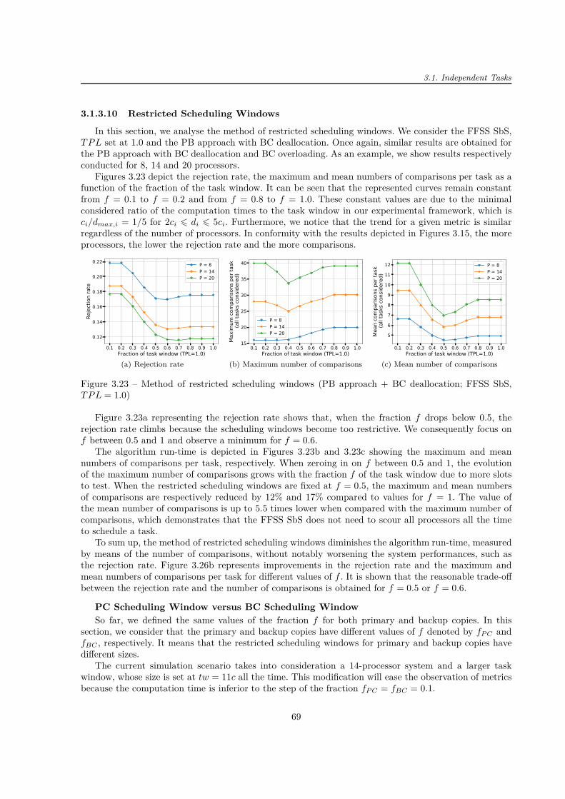
3.1. Independent Tasks

3.1.3.10 Restricted Scheduling Windows

In this section, we analyse the method of restricted scheduling windows. We consider the FFSS SbS,T P L set at 1.0 and the PB approach with BC deallocation. Once again, similar results are obtained forthe PB approach with BC deallocation and BC overloading. As an example, we show results respectivelyconducted for 8, 14 and 20 processors.

Figures 3.23 depict the rejection rate, the maximum and mean numbers of comparisons per task as afunction of the fraction of the task window. It can be seen that the represented curves remain constantfrom f = 0.1 to f = 0.2 and from f = 0.8 to f = 1.0. These constant values are due to the minimalconsidered ratio of the computation times to the task window in our experimental framework, which isci/dmax,i = 1/5 for 2ci 6 di 6 5ci. Furthermore, we notice that the trend for a given metric is similarregardless of the number of processors. In conformity with the results depicted in Figures 3.15, the moreprocessors, the lower the rejection rate and the more comparisons.

0.1 0.2 0.3 0.4 0.5 0.6 0.7 0.8 0.9 1.0Fraction of task window (TPL=1.0)

0.12

0.14

0.16

0.18

0.20

0.22

Reje

ctio

n ra

te

P = 8P = 14P = 20

(a) Rejection rate

0.1 0.2 0.3 0.4 0.5 0.6 0.7 0.8 0.9 1.0Fraction of task window (TPL=1.0)

15

20

25

30

35

40

Max

imum

com

paris

ons p

er ta

sk (a

ll ta

sks c

onsid

ered

)

P = 8P = 14P = 20

(b) Maximum number of comparisons

0.1 0.2 0.3 0.4 0.5 0.6 0.7 0.8 0.9 1.0Fraction of task window (TPL=1.0)

5

6

7

8

9

10

11

12

Mea

n co

mpa

rison

s per

task

(all

task

s con

sider

ed)

P = 8P = 14P = 20

(c) Mean number of comparisons

Figure 3.23 – Method of restricted scheduling windows (PB approach + BC deallocation; FFSS SbS,T P L = 1.0)

Figure 3.23a representing the rejection rate shows that, when the fraction f drops below 0.5, therejection rate climbs because the scheduling windows become too restrictive. We consequently focus onf between 0.5 and 1 and observe a minimum for f = 0.6.

The algorithm run-time is depicted in Figures 3.23b and 3.23c showing the maximum and meannumbers of comparisons per task, respectively. When zeroing in on f between 0.5 and 1, the evolutionof the maximum number of comparisons grows with the fraction f of the task window due to more slotsto test. When the restricted scheduling windows are fixed at f = 0.5, the maximum and mean numbersof comparisons are respectively reduced by 12% and 17% compared to values for f = 1. The value ofthe mean number of comparisons is up to 5.5 times lower when compared with the maximum number ofcomparisons, which demonstrates that the FFSS SbS does not need to scour all processors all the timeto schedule a task.

To sum up, the method of restricted scheduling windows diminishes the algorithm run-time, measuredby means of the number of comparisons, without notably worsening the system performances, such asthe rejection rate. Figure 3.26b represents improvements in the rejection rate and the maximum andmean numbers of comparisons per task for different values of f . It is shown that the reasonable trade-offbetween the rejection rate and the number of comparisons is obtained for f = 0.5 or f = 0.6.

PC Scheduling Window versus BC Scheduling Window

So far, we defined the same values of the fraction f for both primary and backup copies. In thissection, we consider that the primary and backup copies have different values of f denoted by fP C andfBC , respectively. It means that the restricted scheduling windows for primary and backup copies havedifferent sizes.

The current simulation scenario takes into consideration a 14-processor system and a larger taskwindow, whose size is set at tw = 11c all the time. This modification will ease the observation of metricsbecause the computation time is inferior to the step of the fraction fP C = fBC = 0.1.

69

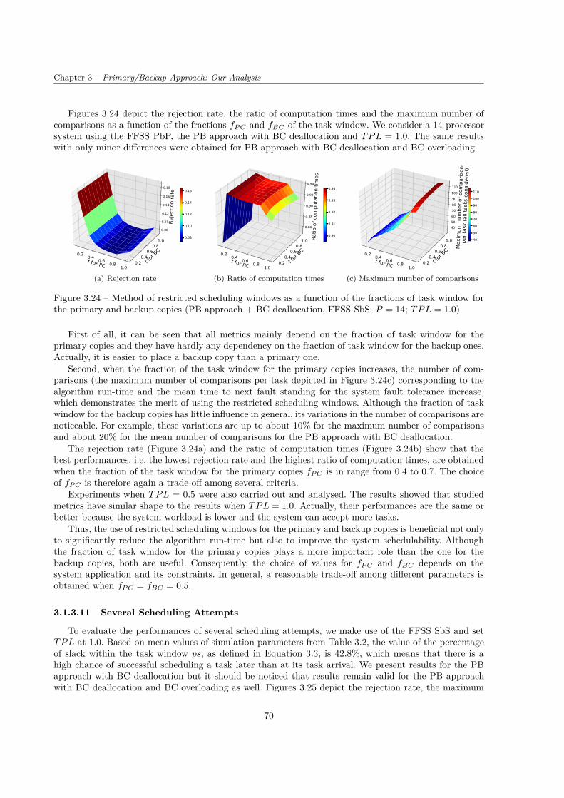
Chapter 3 – Primary/Backup Approach: Our Analysis

Figures 3.24 depict the rejection rate, the ratio of computation times and the maximum number ofcomparisons as a function of the fractions fP C and fBC of the task window. We consider a 14-processorsystem using the FFSS PbP, the PB approach with BC deallocation and T P L = 1.0. The same resultswith only minor differences were obtained for PB approach with BC deallocation and BC overloading.

f for PC

0.2 0.4 0.6 0.81.0

f for BC

0.20.4

0.60.8

1.0

Rejection rate

0.08

0.10

0.12

0.14

0.16

0.18

0.08

0.10

0.12

0.14

0.16

(a) Rejection rate

f for PC

0.2 0.4 0.6 0.81.0

f for BC

0.20.4

0.60.8

1.0 Ratio

of c

ompu

tatio

n tim

es

0.86

0.88

0.90

0.92

0.94

0.90

0.91

0.92

0.93

0.94

(b) Ratio of computation times

f for PC

0.2 0.4 0.6 0.81.0

f for B

C

0.20.4

0.60.8

1.0

Max

imum

num

ber o

f com

paris

ons

per

task

(all

task

s con

sider

ed)

405060708090100110

40

50

60

70

80

90

100

110

(c) Maximum number of comparisons

Figure 3.24 – Method of restricted scheduling windows as a function of the fractions of task window forthe primary and backup copies (PB approach + BC deallocation, FFSS SbS; P = 14; T P L = 1.0)

First of all, it can be seen that all metrics mainly depend on the fraction of task window for theprimary copies and they have hardly any dependency on the fraction of task window for the backup ones.Actually, it is easier to place a backup copy than a primary one.

Second, when the fraction of the task window for the primary copies increases, the number of com-parisons (the maximum number of comparisons per task depicted in Figure 3.24c) corresponding to thealgorithm run-time and the mean time to next fault standing for the system fault tolerance increase,which demonstrates the merit of using the restricted scheduling windows. Although the fraction of taskwindow for the backup copies has little influence in general, its variations in the number of comparisons arenoticeable. For example, these variations are up to about 10% for the maximum number of comparisonsand about 20% for the mean number of comparisons for the PB approach with BC deallocation.

The rejection rate (Figure 3.24a) and the ratio of computation times (Figure 3.24b) show that thebest performances, i.e. the lowest rejection rate and the highest ratio of computation times, are obtainedwhen the fraction of the task window for the primary copies fP C is in range from 0.4 to 0.7. The choiceof fP C is therefore again a trade-off among several criteria.

Experiments when T P L = 0.5 were also carried out and analysed. The results showed that studiedmetrics have similar shape to the results when T P L = 1.0. Actually, their performances are the same orbetter because the system workload is lower and the system can accept more tasks.

Thus, the use of restricted scheduling windows for the primary and backup copies is beneficial not onlyto significantly reduce the algorithm run-time but also to improve the system schedulability. Althoughthe fraction of task window for the primary copies plays a more important role than the one for thebackup copies, both are useful. Consequently, the choice of values for fP C and fBC depends on thesystem application and its constraints. In general, a reasonable trade-off among different parameters isobtained when fP C = fBC = 0.5.

3.1.3.11 Several Scheduling Attempts

To evaluate the performances of several scheduling attempts, we make use of the FFSS SbS and setT P L at 1.0. Based on mean values of simulation parameters from Table 3.2, the value of the percentageof slack within the task window ps, as defined in Equation 3.3, is 42.8%, which means that there is ahigh chance of successful scheduling a task later than at its task arrival. We present results for the PBapproach with BC deallocation but it should be noticed that results remain valid for the PB approachwith BC deallocation and BC overloading as well. Figures 3.25 depict the rejection rate, the maximum

70

3.1. Independent Tasks

and mean numbers of comparisons per task as a function of the number of processors when ω = 25% andω = 33%.

2 4 6 8 10 12 14 16 18 20 22 24Number of processors (TPL = 1.0)

0.10

0.15

0.20

0.25

0.30

0.35

Rejection rate

(a) Rejection rate

2 4 6 8 10 12 14 16 18 20 22 24Number of processors (TPL = 1.0)

10

20

30

40

50

Max

imum

num

ber c

ompa

rison

s per ta

sk(all task

s con

sidered

)

(b) Maximum number of comparisons

2 4 6 8 10 12 14 16 18 20 22 24Number of processors (TPL = 1.0)

2

3

4

5

6

7

8

9

10

Mean number c

omparisons p

er ta

sk (a

ll tasks c

onsid

ered)

(c) Mean number of comparisons

Figure 3.25 – Method of several scheduling attempts (PB approach + BC deallocation, FFSS SbS,T P L = 1.0)

As it can be seen in Figure 3.25a, two or three scheduling attempts are always beneficial and thedecrease in the rejection rate is respectively about 6% or 7%. The maximum and mean numbers ofcomparisons per task, respectively depicted in Figures 3.25b and 3.25c, are worsened when compared tothe algorithm carrying out only one scheduling attempt because every new attempt requires additionalcomparisons.

Figure 3.26c showing the improvement for a 14-processor system sums up the results. It is worthnoticing it is no good trying more than two attempts because we can hardly expect any improvement inthe rejection rate and the number of comparisons is higher. The reasonable trade-off between the rejectionrate and the number of comparisons is the use of two scheduling attempts at 33% of the task window.

3P/2 P P/2 P/3 P/4Number of authorised com arisons for PC (5 com arisons for BC)

−20

0

20

40

60

Im rovem

ent (

%)

Rejection rateMax # comp.Mean # comp.

(a) Limitation on the number of comparisons

f=0.4 f=0.5 f=0.6 f=0.7Fraction of task window

−15

−10

−5

0

5

10

15

Impro

emen

t (%)

Rejection rateMax # comparisonsMean # comparisons

(b) Restricted scheduling windows

2 (ω=25%) 2 (ω=33%) 3 (ω=25%) 3 (ω=33%)Number and po ition of cheduling attempt

%25

%20

%15

%10

%5

0

5

Impr

ovem

ent (

%)

Rejection rateMax # comp.Mean # comp.

(c) Several scheduling attempts

Figure 3.26 – Improvements to a 14-processor system compared to the PB approach without proposedenhancing methods (PB with BC deallocation; FFSS SbS; T P L = 1.0)

3.1.3.12 Combination of Enhancing Methods

We remind the reader that our aim is to significantly reduce the number of comparisons withoutworsening the rejection rate. Consequently, we analyse the aforementioned methods (and their combi-nations) employing the parameters that achieve the best performances from the viewpoint of both thenumber of comparisons and the rejection rate. The values of these parameters are based on the results

71

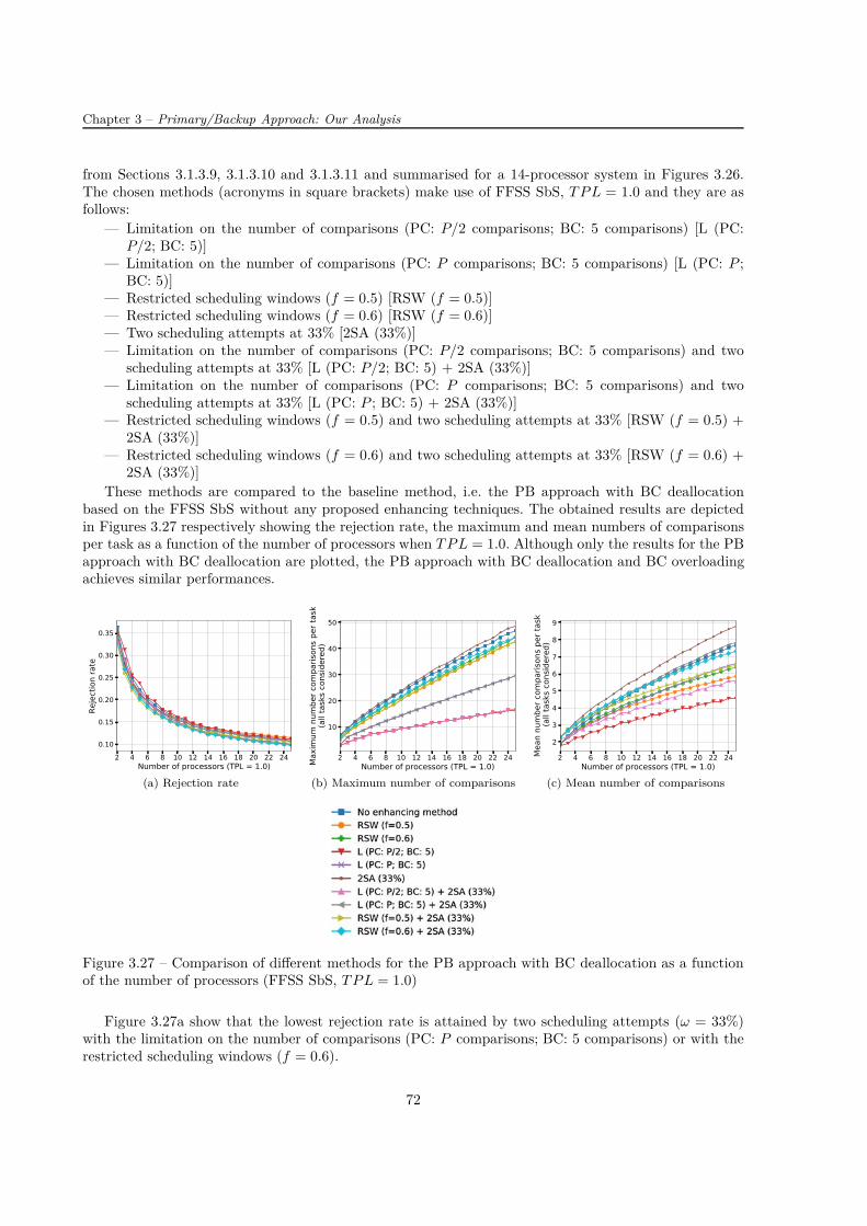
Chapter 3 – Primary/Backup Approach: Our Analysis

from Sections 3.1.3.9, 3.1.3.10 and 3.1.3.11 and summarised for a 14-processor system in Figures 3.26.The chosen methods (acronyms in square brackets) make use of FFSS SbS, T P L = 1.0 and they are asfollows:

— Limitation on the number of comparisons (PC: P/2 comparisons; BC: 5 comparisons) [L (PC:P/2; BC: 5)]

— Limitation on the number of comparisons (PC: P comparisons; BC: 5 comparisons) [L (PC: P ;BC: 5)]

— Restricted scheduling windows (f = 0.5) [RSW (f = 0.5)]— Restricted scheduling windows (f = 0.6) [RSW (f = 0.6)]— Two scheduling attempts at 33% [2SA (33%)]— Limitation on the number of comparisons (PC: P/2 comparisons; BC: 5 comparisons) and two

scheduling attempts at 33% [L (PC: P/2; BC: 5) + 2SA (33%)]— Limitation on the number of comparisons (PC: P comparisons; BC: 5 comparisons) and two

scheduling attempts at 33% [L (PC: P ; BC: 5) + 2SA (33%)]— Restricted scheduling windows (f = 0.5) and two scheduling attempts at 33% [RSW (f = 0.5) +

2SA (33%)]— Restricted scheduling windows (f = 0.6) and two scheduling attempts at 33% [RSW (f = 0.6) +

2SA (33%)]These methods are compared to the baseline method, i.e. the PB approach with BC deallocation

based on the FFSS SbS without any proposed enhancing techniques. The obtained results are depictedin Figures 3.27 respectively showing the rejection rate, the maximum and mean numbers of comparisonsper task as a function of the number of processors when T P L = 1.0. Although only the results for the PBapproach with BC deallocation are plotted, the PB approach with BC deallocation and BC overloadingachieves similar performances.

2 4 6 8 10 12 14 16 18 20 22 24Number of processors (TPL = 1.0)

0.10

0.15

0.20

0.25

0.30

0.35

Rejection rate

(a) Rejection rate

2 4 6 8 10 12 14 16 18 20 22 24Number of processors (TPL = 1.0)

10

20

30

40

50

Max

imum

num

ber c

ompa

rison

s per ta

sk(all task

s con

sidered

)

(b) Maximum number of comparisons

2 4 6 8 10 12 14 16 18 20 22 24Number of processors (TPL = 1.0)

2

3

4

5

6

7

8

9

Mean number c

omparisons p

er ta

sk (a

ll tasks c

onsid

ered)

(c) Mean number of comparisons

Figure 3.27 – Comparison of different methods for the PB approach with BC deallocation as a functionof the number of processors (FFSS SbS, T P L = 1.0)

Figure 3.27a show that the lowest rejection rate is attained by two scheduling attempts (ω = 33%)with the limitation on the number of comparisons (PC: P comparisons; BC: 5 comparisons) or with therestricted scheduling windows (f = 0.6).

72

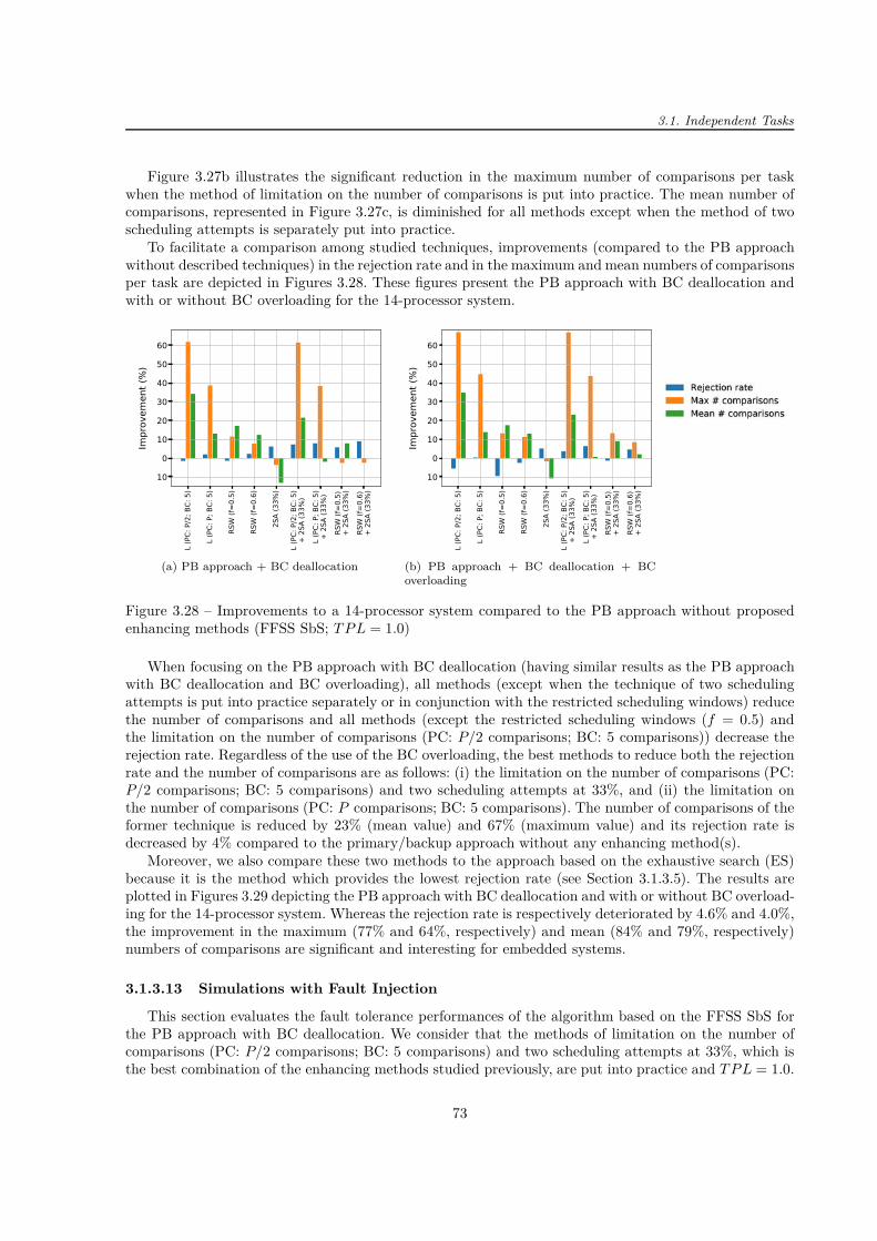
3.1. Independent Tasks

Figure 3.27b illustrates the significant reduction in the maximum number of comparisons per taskwhen the method of limitation on the number of comparisons is put into practice. The mean number ofcomparisons, represented in Figure 3.27c, is diminished for all methods except when the method of twoscheduling attempts is separately put into practice.

To facilitate a comparison among studied techniques, improvements (compared to the PB approachwithout described techniques) in the rejection rate and in the maximum and mean numbers of comparisonsper task are depicted in Figures 3.28. These figures present the PB approach with BC deallocation andwith or without BC overloading for the 14-processor system.

L (P

C: P

/2; B

C: 5

)

L (P

C: P

; BC:

5)

RSW

(f=0

.5)

RSW

(f=0

.6)

2SA

(33%

)

L (P

C: P

/2; B

C: 5

)+

2SA

(33%

)L

(PC:

P; B

C: 5

)+

2SA

(33%

)RS

W (f

=0.5

)+

2SA

(33%

)RS

W (f

=0.6

)+

2SA

(33%

)

−10

0

10

20

30

40

50

60

Imp

ovem

ent (

%)

(a) PB approach + BC deallocation

L (P

C: P

/2; B

C: 5

)

L (P

C: P

; BC:

5)

RSW

(f=0

.5)

RSW

(f=0

.6)

2SA

(33%

)

L (P

C: P

/2; B

C: 5

)+

2SA

(33%

)L

(PC:

P; B

C: 5

)+

2SA

(33%

)RS

W (f

=0.5

)+

2SA

(33%

)RS

W (f

=0.6

)+

2SA

(33%

)

−10

0

10

20

30

40

50

60

Imp

ovem

ent (

%)

(b) PB approach + BC deallocation + BCoverloading

Figure 3.28 – Improvements to a 14-processor system compared to the PB approach without proposedenhancing methods (FFSS SbS; T P L = 1.0)

When focusing on the PB approach with BC deallocation (having similar results as the PB approachwith BC deallocation and BC overloading), all methods (except when the technique of two schedulingattempts is put into practice separately or in conjunction with the restricted scheduling windows) reducethe number of comparisons and all methods (except the restricted scheduling windows (f = 0.5) andthe limitation on the number of comparisons (PC: P/2 comparisons; BC: 5 comparisons)) decrease therejection rate. Regardless of the use of the BC overloading, the best methods to reduce both the rejectionrate and the number of comparisons are as follows: (i) the limitation on the number of comparisons (PC:P/2 comparisons; BC: 5 comparisons) and two scheduling attempts at 33%, and (ii) the limitation onthe number of comparisons (PC: P comparisons; BC: 5 comparisons). The number of comparisons of theformer technique is reduced by 23% (mean value) and 67% (maximum value) and its rejection rate isdecreased by 4% compared to the primary/backup approach without any enhancing method(s).

Moreover, we also compare these two methods to the approach based on the exhaustive search (ES)because it is the method which provides the lowest rejection rate (see Section 3.1.3.5). The results areplotted in Figures 3.29 depicting the PB approach with BC deallocation and with or without BC overload-ing for the 14-processor system. Whereas the rejection rate is respectively deteriorated by 4.6% and 4.0%,the improvement in the maximum (77% and 64%, respectively) and mean (84% and 79%, respectively)numbers of comparisons are significant and interesting for embedded systems.

3.1.3.13 Simulations with Fault Injection

This section evaluates the fault tolerance performances of the algorithm based on the FFSS SbS forthe PB approach with BC deallocation. We consider that the methods of limitation on the number ofcomparisons (PC: P/2 comparisons; BC: 5 comparisons) and two scheduling attempts at 33%, which isthe best combination of the enhancing methods studied previously, are put into practice and T P L = 1.0.

73

Chapter 3 – Primary/Backup Approach: Our Analysis

L (P

C: P

/2; B

C: 5

)

L (P

C: P

; BC:

5)

RSW

(f=0

.5)

RSW

(f=0

.6)

2SA

(33%

)

L (P

C: P

/2; B

C: 5

) +

2SA

(33%

)L

(PC:

P; B

C: 5

) +

2SA

(33%

)RS

W (f

=0.5

) +

2SA

(33%

)RS

W (f

=0.6

) +

2SA

(33%

)−20

0

20

40

60

80

Imp

ovem

ent (

%)

(a) PB approach + BC deallocationL

(PC:

P/2

; BC:

5)

L (P

C: P

; BC:

5)

RSW

(f=0

.5)

RSW

(f=0

.6)

2SA

(33%

)

L (P

C: P

/2; B

C: 5

) +

2SA

(33%

)L

(PC:

P; B

C: 5

) +

2SA

(33%

)RS

W (f

=0.5

) +

2SA

(33%

)RS

W (f

=0.6

) +

2SA

(33%

)−20

0

20

40

60

80

Imp

ovem

ent (

%)

(b) PB approach + BC deallocation + BCoverloading

Figure 3.29 – Improvements to a 14-processor system using FFSS SbS compared to the PB approachusing ES without proposed enhancing methods (T P L = 1.0)

It should be noticed that the conclusions made for this case are also valid for other techniques withand without BC deallocation and/or BC overloading. The only difference is related to the rejection ratewhen the BC deallocation is not put into practice. Actually, when the BC deallocation is not used, therejection rate remains the same regardless of the value of fault rates because all tasks copies are scheduledand no backup copy is deallocated. Consequently, such a system has the same performances from thepoint of view of the system schedulability.

Figures 3.30 depict the total number of faults against the number of processors, while the totalnumber is the sum of the faults without impact, faults impacting simple tasks and faults impactingdouble tasks. The fault rates injected per processor and represented in the figures respectively equal1 · 10−5 fault/ms (corresponding to the worst estimated fault rate in a harsh environment [118]), 4 · 10−4

fault/ms (corresponding to the limit of the assumption of only one fault in the system at the same timefor a 25-processor system) and 1 · 10−2 fault/ms.

2 4 6 8 10 12 14 16 18 20 22 24Number of processors

0.0

0.2

0.4

0.6

0.8

1.0

1.2

Numbe

r

Faults without impactFaults impacting PCFaults impacting BC

(a) 1 · 10−5 fault/ms

2 4 6 8 10 12 14 16 18 20 22 24Number of processors

0

10

20

30

40

Numbe

r

Faults without impactFaults impacting PCFaults impacting BC

(b) 4 · 10−4 fault/ms

2 4 6 8 10 12 14 16 18 20 22 24Number of processors

0

200

400

600

800

1000

Numbe

r

Faults without impactFaults impacting PCFaults impacting BC

(c) 1 · 10−2 fault/ms

Figure 3.30 – Total number of faults (injected with a given fault rate per processor) against the numberof processors (PB approach + BC deallocation (FFSS SbS) with limitation on the number of comparisons(PC: P/2 comparisons; BC: 5 comparisons) and two scheduling attempts at 33%)

The number of impacted tasks is directly proportional to the processor load, represented in Fig-ure 3.15b. When the rate of injected faults per processor increases, there are more impacted task copiesas well. Furthermore, while the number of impacted backup copies is negligible when compared to theone of primary copies, there are more backup copies impacted when the fault injection rates are higher.

74

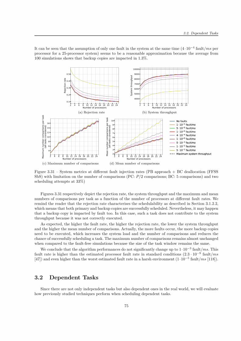
3.2. Dependent Tasks

It can be seen that the assumption of only one fault in the system at the same time (4 ·10−4 fault/ms perprocessor for a 25-processor system) seems to be a reasonable approximation because the average from100 simulations shows that backup copies are impacted in 1.3%.

2 4 6 8 10 12 14 16 18 20 22 24Number of processors

0.1

0.2

0.3

0.4

0.5

Rejection rate

(a) Rejection rate

2 4 6 8 10 12 14 16 18 20 22 24Number of processors

4000

5000

6000

7000

8000

9000

10000

System

throug

hput

(b) System throughput

2 4 6 8 10 12 14 16 18 20 22 24Number of processors

4

6

8

10

12

14

16

Max

imum

num

ber c

ompa

rison

s per ta

sk(all tasks c

onsid

ered

)

(c) Maximum number of comparisons

2 4 6 8 10 12 14 16 18 20 22 24Number of processors

2

3

4

5

6

7

8

9

10

Mea

n nu

mbe

r com

paris

ons p

er ta

sk (a

ll tasks c

onsid

ered

)

(d) Mean number of comparisons

Figure 3.31 – System metrics at different fault injection rates (PB approach + BC deallocation (FFSSSbS) with limitation on the number of comparisons (PC: P/2 comparisons; BC: 5 comparisons) and twoscheduling attempts at 33%)

Figures 3.31 respectively depict the rejection rate, the system throughput and the maximum and meannumbers of comparisons per task as a function of the number of processors at different fault rates. Weremind the reader that the rejection rate characterises the schedulability as described in Section 3.1.2.2,which means that both primary and backup copies are successfully scheduled. Nevertheless, it may happenthat a backup copy is impacted by fault too. In this case, such a task does not contribute to the systemthroughput because it was not correctly executed.

As expected, the higher the fault rate, the higher the rejection rate, the lower the system throughputand the higher the mean number of comparisons. Actually, the more faults occur, the more backup copiesneed to be executed, which increases the system load and the number of comparisons and reduces thechance of successfully scheduling a task. The maximum number of comparisons remains almost unchangedwhen compared to the fault-free simulations because the size of the task window remains the same.

We conclude that the algorithm performances do not significantly change up to 1 ·10−3 fault/ms. Thisfault rate is higher than the estimated processor fault rate in standard conditions (2.3 · 10−9 fault/ms[47]) and even higher than the worst estimated fault rate in a harsh environment (1 ·10−5 fault/ms [118]).

3.2 Dependent Tasks

Since there are not only independent tasks but also dependent ones in the real world, we will evaluatehow previously studied techniques perform when scheduling dependent tasks.

75

Chapter 3 – Primary/Backup Approach: Our Analysis

3.2.1 Assumptions and Scheduling Model

All assumptions and models presented in Section 3.1.1 remain valid.We call the application a set of dependent tasks that can be modelled by a directed acyclic graph

(DAG). An example is depicted in Figure 3.32.

Figure 3.32 – Example of a general directed acyclic graph (DAG)

A DAG is characterised by the nodes and directed edges between the nodes that represent tasksand their dependencies, respectively. The DAG attributes are as follows: arrival time aDAG, deadlinedDAG, attributes for each node and attributes for each edges. The node attributes correspond to the taskcharacteristics defined for independent tasks and which are as reads: arrival time ai, computation timeci and deadline di. Regarding the attributes related to edges, there are characterised by the origin anddestination nodes. In this work, we do not take into account communication times.

According to Graham’s notation [66] described in Section 1.1, the studied problem is defined as follows:

P ; m | n = k; prec; online rj ; dj = d; pj = p | (check the feasibility of schedule)

which means that k dependent jobs/tasks (characterised by release time rj , processing time pj anddeadline dj) arrive online on a system consisting of m parallel identical machines and are scheduled toverify the feasibility of a schedule. The algorithm is online global and clairvoyant.

3.2.2 Scheduling Methods

In this manuscript, we do not introduce scheduling methods solely meant for dependent tasks butwe make use of the ones already used for independent tasks. This section overviews the methods weimplemented for dependent tasks.

We concluded that both the BC deallocation and the BC overloading improve the schedulabilitywhen dealing with independent tasks. Consequently, when scheduling dependent tasks, we only analysethe method using the PB approach with BC deallocation and BC overloading. Regarding the schedulingsearch techniques and processor allocation policies employed to find a slot big enough to place a taskcopy, we evaluate the following strategies:

— Free Slot Search Technique + First Found Solution First: Processor by Processor (FSST + FFSSPbP)

— Free Slot Search Technique + First Found Solution First: Slot by Slot (FSST + FFSS SbS)— Boundary Schedule Search Technique + ES: BC scheduled ASAP (BSST + ES BC ASAP)— Boundary Schedule Search Technique + ES: BC scheduled with maximum overloading (BSST +

ES BC maxOverload)The description of processor allocation policies is given in Section 3.1.1.2 and the principle of schedul-

ing search techniques is presented in Section 3.1.1.3. There is no difference in principles of these methodswhen scheduling independent or dependent tasks except one. The only modification is that the backupcopies of dependent tasks are placed as soon as possible in order not to delay computations in the case afault occurs during an execution of a primary copy. Nevertheless, the studied approach remains passive,i.e. the primary and backup copies of the same task cannot be executed at the same time. Table 3.3 sumsup the position of task copies for studied methods. A search to find a slot large enough for a task copy

76

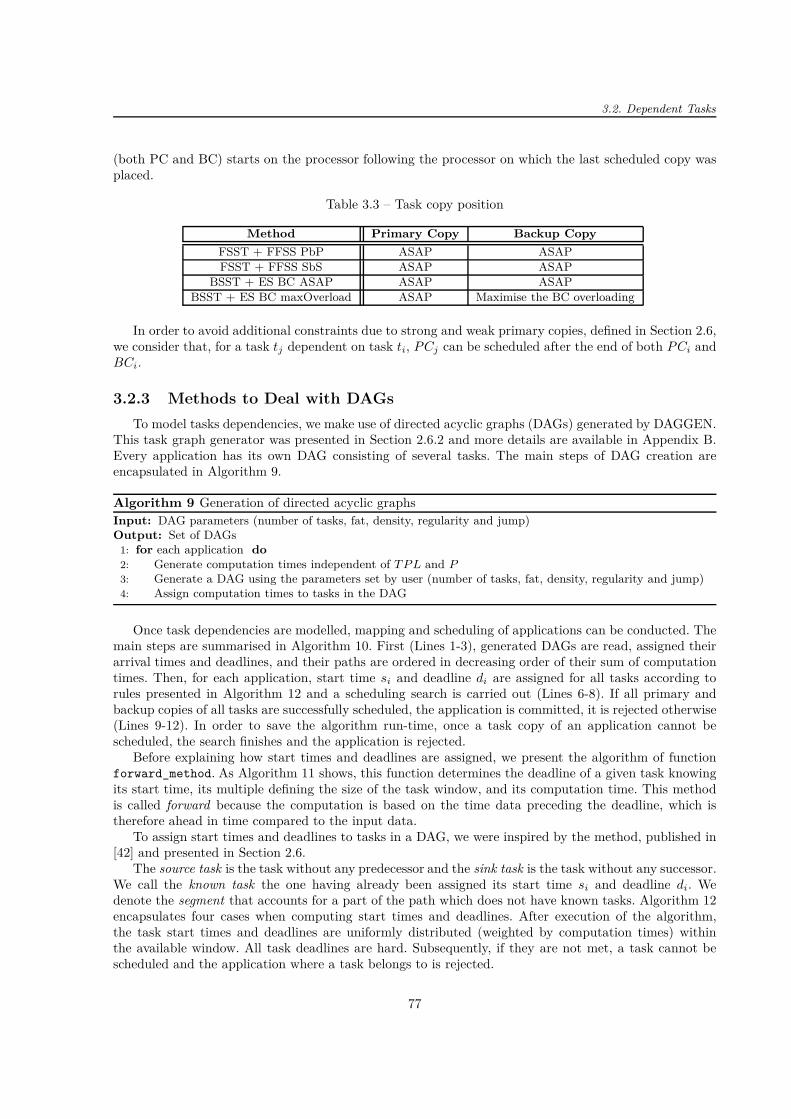
3.2. Dependent Tasks

(both PC and BC) starts on the processor following the processor on which the last scheduled copy wasplaced.

Table 3.3 – Task copy position

Method Primary Copy Backup Copy

FSST + FFSS PbP ASAP ASAP

FSST + FFSS SbS ASAP ASAP

BSST + ES BC ASAP ASAP ASAP

BSST + ES BC maxOverload ASAP Maximise the BC overloading

In order to avoid additional constraints due to strong and weak primary copies, defined in Section 2.6,we consider that, for a task tj dependent on task ti, P Cj can be scheduled after the end of both P Ci andBCi.

3.2.3 Methods to Deal with DAGs

To model tasks dependencies, we make use of directed acyclic graphs (DAGs) generated by DAGGEN.This task graph generator was presented in Section 2.6.2 and more details are available in Appendix B.Every application has its own DAG consisting of several tasks. The main steps of DAG creation areencapsulated in Algorithm 9.

Algorithm 9 Generation of directed acyclic graphsInput: DAG parameters (number of tasks, fat, density, regularity and jump)Output: Set of DAGs

1: for each application do2: Generate computation times independent of T P L and P3: Generate a DAG using the parameters set by user (number of tasks, fat, density, regularity and jump)4: Assign computation times to tasks in the DAG

Once task dependencies are modelled, mapping and scheduling of applications can be conducted. Themain steps are summarised in Algorithm 10. First (Lines 1-3), generated DAGs are read, assigned theirarrival times and deadlines, and their paths are ordered in decreasing order of their sum of computationtimes. Then, for each application, start time si and deadline di are assigned for all tasks according torules presented in Algorithm 12 and a scheduling search is carried out (Lines 6-8). If all primary andbackup copies of all tasks are successfully scheduled, the application is committed, it is rejected otherwise(Lines 9-12). In order to save the algorithm run-time, once a task copy of an application cannot bescheduled, the search finishes and the application is rejected.

Before explaining how start times and deadlines are assigned, we present the algorithm of functionforward_method. As Algorithm 11 shows, this function determines the deadline of a given task knowingits start time, its multiple defining the size of the task window, and its computation time. This methodis called forward because the computation is based on the time data preceding the deadline, which istherefore ahead in time compared to the input data.

To assign start times and deadlines to tasks in a DAG, we were inspired by the method, published in[42] and presented in Section 2.6.

The source task is the task without any predecessor and the sink task is the task without any successor.We call the known task the one having already been assigned its start time si and deadline di. Wedenote the segment that accounts for a part of the path which does not have known tasks. Algorithm 12encapsulates four cases when computing start times and deadlines. After execution of the algorithm,the task start times and deadlines are uniformly distributed (weighted by computation times) withinthe available window. All task deadlines are hard. Subsequently, if they are not met, a task cannot bescheduled and the application where a task belongs to is rejected.

77

Chapter 3 – Primary/Backup Approach: Our Analysis

Algorithm 10 Main steps to schedule dependent tasksInput: Set of DAGsOutput: Mapping and scheduling MS of scheduled DAGs

1: Read generated DAGs2: Compute the length of all paths and sort them in decreasing order3: Generate DAG arrival time (dependent on T P L and P ) and deadline4: for each application do5: Assign start time si and deadline di for all tasks according to rules presented in Algorithm 126: for each task do7: Search for PC slot8: Search for BC slot9: if PC and BC of each task exist then

10: Commit the application11: else12: Reject the application

Algorithm 11 Forward method to determine a deadlineInput: Start time s, Multiple 6α, Computation time cOutput: Deadline d

1: d = s + α · c

In order to improve the schedulability, once PC and BC slots of a task are determined, the start timesof their direct children are set. This makes the task windows larger and increases the probability to finda slot large enough to place a task copy.

To illustrate this stage, we consider an application represented by a DAG depicted in Figure 3.33.Each task was given a computation time as noted in the second column in Table 3.4. All task start timesand deadlines were computed using Algorithm 12. The results are gathered in Table 3.4.

6. A multiple α is an integer at least equal to 2 in order to be able to schedule both primary and backup copies withinthe task window without their overlap. The value of α is the same as for the whole DAG.

78

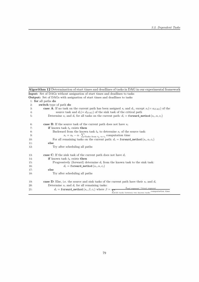
3.2. Dependent Tasks

Algorithm 12 Determination of start times and deadlines of tasks in DAG in our experimental frameworkInput: Set of DAGs without assignation of start times and deadlines to tasksOutput: Set of DAGs with assignation of start times and deadlines to tasks

1: for all paths do2: switch type of path do3: case A: If no task on the current path has been assigned si and di, except si(= aDAG) of the4: source task and di(= dDAG) of the sink task of the critical path5: Determine si and di for all tasks on the current path: di = forward_method (si, α, ci)

6: case B: If the source task of the current path does not have si

7: if known task tk exists then8: Backward from the known task tk to determine si of the source task:9: si = sk − α ·

∑

Tasks from tk to ticomputation time

10: For all remaining tasks on the current path: di = forward_method (si, α, ci)11: else12: Try after scheduling all paths

13: case C: If the sink task of the current path does not have di

14: if known task tk exists then15: Progressively (forward) determine di from the known task to the sink task:16: di = forward_method (si, α, ci)17: else18: Try after scheduling all paths

19: case D: Else, i.e. the source and sink tasks of the current path have their si and di

20: Determine si and di for all remaining tasks:

21: di = forward_method (si, β, ci) where β =dend segment−sstart segment

∑

All tasks between two known taskscomputation time

79

Chapter 3 – Primary/Backup Approach: Our Analysis

0

8

1 1

1

2

3 5 6

4

9

7

1 0

1 21 3

1 4

2 0

1 5

1 6

1 71 8

1 9

Figure 3.33 – Example of a DAG

Table 3.4 – Example of tasks (belonging to the DAG depicted in Figure 3.33) with their computationtimes and assigned start times and deadlines

Task ti Computation time ci Start time si Deadline di

0 65 d0 − α · c0 s20 − α · (c8 + c11 + c13 + c15 + c17 + c19)

1 15 aDAG forward_method (s1, α, c1)

2 1 5 end(BC1) forward_method (s2, α, c2)

3 15 end(BC2) forward_method (s3, α, c3)

4 15 end(BC3) forward_method (s4, α, c4)

5 7 end(BC2) s9

6 3 end(BC2) forward_method(

s6, s9−d2c6+c7

, c6

)

7 2 end(BC6) s9

8 5 end(BC0) forward_method (s8, α, c8)

9 15 end(BC4) forward_method (s9, α, c9)

10 15 end(BC9) forward_method (s10, α, c10)

11 40 end(BC8) forward_method (s11, α, c11)

12 15 end(BC11) forward_method (s12, α, c12)

13 5 end(BC11) forward_method (s13, α, c13)

14 15 end(BC10) forward_method (s14, α, c14)

15 4 end(BC13) forward_method (s15, α, c15)

16 3 end(BC15) forward_method(

s16, s19−d15c16+c18

, c16

)

17 5 end(BC15) forward_method (s17, α, c17)

18 1 end(BC18) s19

19 5 end(BC17) forward_method (s19, α, c19)

20 15 end(BC14) dDAG

80

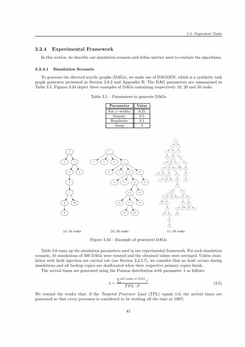
3.2. Dependent Tasks

3.2.4 Experimental Framework

In this section, we describe our simulation scenario and define metrics used to evaluate the algorithms.

3.2.4.1 Simulation Scenario

To generate the directed acyclic graphs (DAGs), we make use of DAGGEN, which is a synthetic taskgraph generator presented in Section 2.6.2 and Appendix B. The DAG parameters are summarised inTable 3.5. Figures 3.34 depict three examples of DAGs containing respectively 10, 20 and 50 tasks.

Table 3.5 – Parameters to generate DAGs

Parameter Value

Fat (=width) 0.25

Density 0.5

Regularity 0.1

Jump 3

(a) 10 tasks

1

2 3 4 5

6 7 8 1 0

9 1 1 1 2 1 5

1 3 1 4

1 6 1 7 1 8

1 9 2 0

(b) 20 tasks

1

2 3

45 7

681 0

1 2

1 39 1 11 4

1 61 5 1 8 1 9

2 11 7 2 0 2 2 2 3

2 42 52 7 2 8 2 6

2 9

3 0 3 4

3 1 3 23 3

3 5

3 8 3 9

3 6

3 7

4 1 4 0

4 24 3

4 8

4 44 7 4 54 6

5 0

4 9

(c) 50 tasks

Figure 3.34 – Example of generated DAGs

Table 3.6 sums up the simulation parameters used in our experimental framework. For each simulationscenario, 10 simulations of 500 DAGs were treated and the obtained values were averaged. Unless simu-lation with fault injection are carried out (see Section 3.2.5.7), we consider that no fault occurs duringsimulations and all backup copies are deallocated when their respective primary copies finish.

The arrival times are generated using the Poisson distribution with parameter λ as follows:

λ =∑all tasks in DAG

c

T P L · P(3.5)

We remind the reader that, if the Targeted Processor Load (TPL) equals 1.0, the arrival times aregenerated so that every processor is considered to be working all the time at 100%.

81

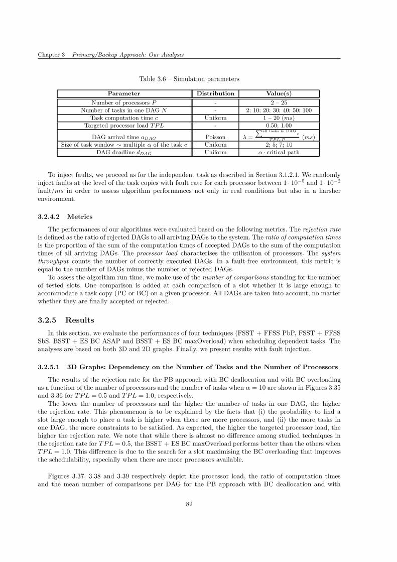
Chapter 3 – Primary/Backup Approach: Our Analysis

Table 3.6 – Simulation parameters

Parameter Distribution Value(s)

Number of processors P - 2 – 25

Number of tasks in one DAG N - 2; 10; 20; 30; 40; 50; 100

Task computation time c Uniform 1 – 20 (ms)

Targeted processor load T P L - 0.50; 1.00

DAG arrival time aDAG Poisson λ =

∑

all tasks in DAGc

T P L·P(ms)

Size of task window ∼ multiple α of the task c Uniform 2; 5; 7; 10

DAG deadline dDAG Uniform α · critical path

To inject faults, we proceed as for the independent task as described in Section 3.1.2.1. We randomlyinject faults at the level of the task copies with fault rate for each processor between 1 · 10−5 and 1 · 10−2

fault/ms in order to assess algorithm performances not only in real conditions but also in a harsherenvironment.

3.2.4.2 Metrics

The performances of our algorithms were evaluated based on the following metrics. The rejection rateis defined as the ratio of rejected DAGs to all arriving DAGs to the system. The ratio of computation timesis the proportion of the sum of the computation times of accepted DAGs to the sum of the computationtimes of all arriving DAGs. The processor load characterises the utilisation of processors. The systemthroughput counts the number of correctly executed DAGs. In a fault-free environment, this metric isequal to the number of DAGs minus the number of rejected DAGs.

To assess the algorithm run-time, we make use of the number of comparisons standing for the numberof tested slots. One comparison is added at each comparison of a slot whether it is large enough toaccommodate a task copy (PC or BC) on a given processor. All DAGs are taken into account, no matterwhether they are finally accepted or rejected.

3.2.5 Results

In this section, we evaluate the performances of four techniques (FSST + FFSS PbP, FSST + FFSSSbS, BSST + ES BC ASAP and BSST + ES BC maxOverload) when scheduling dependent tasks. Theanalyses are based on both 3D and 2D graphs. Finally, we present results with fault injection.

3.2.5.1 3D Graphs: Dependency on the Number of Tasks and the Number of Processors

The results of the rejection rate for the PB approach with BC deallocation and with BC overloadingas a function of the number of processors and the number of tasks when α = 10 are shown in Figures 3.35and 3.36 for T P L = 0.5 and T P L = 1.0, respectively.

The lower the number of processors and the higher the number of tasks in one DAG, the higherthe rejection rate. This phenomenon is to be explained by the facts that (i) the probability to find aslot large enough to place a task is higher when there are more processors, and (ii) the more tasks inone DAG, the more constraints to be satisfied. As expected, the higher the targeted processor load, thehigher the rejection rate. We note that while there is almost no difference among studied techniques inthe rejection rate for T P L = 0.5, the BSST + ES BC maxOverload performs better than the others whenT P L = 1.0. This difference is due to the search for a slot maximising the BC overloading that improvesthe schedulability, especially when there are more processors available.

Figures 3.37, 3.38 and 3.39 respectively depict the processor load, the ratio of computation timesand the mean number of comparisons per DAG for the PB approach with BC deallocation and with

82

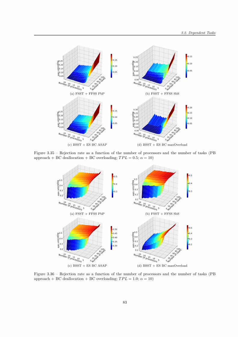
3.2. Dependent Tasks

Numb

er of tasks

020

4060

80100

Number of processors 510152025

Rejection rate

0.050.100.150.200.25

0.05

0.10

0.15

(a) FSST + FFSS PbP

Numb

er of tasks

020

4060

80100

Number of processors 510152025

Rejection rate

0.00

0.05

0.10

0.15

0.20

0.25

0.05

0.10

0.15

(b) FSST + FFSS SbS

Numb

er of tasks

020

4060

80100

Number of processors 510152025

Rejection rate

0.050.100.150.200.25

0.05

0.10

0.15

(c) BSST + ES BC ASAP

Numb

er of tasks

020

4060

80100

Number of processors 510152025

Rejection rate

0.000.050.100.150.200.250.30

0.05

0.10

0.15

0.20

(d) BSST + ES BC maxOverload

Figure 3.35 – Rejection rate as a function of the number of processors and the number of tasks (PBapproach + BC deallocation + BC overloading; T P L = 0.5; α = 10)

Numb

er of tasks

020

4060

80100

Number of processors 510152025

Rejection rate

0.2

0.3

0.4

0.5

0.3

0.4

0.5

(a) FSST + FFSS PbP

Numb

er of tasks

020

4060

80100

Number of processors 510152025

Rejection rate

0.1

0.2

0.3

0.4

0.5

0.3

0.4

0.5

(b) FSST + FFSS SbS

Numb

er of tasks

020

4060

80100

Number of processors 510152025

Rejection rate

0.2

0.3

0.4

0.5

0.30

0.35

0.40

0.45

0.50

(c) BSST + ES BC ASAP

Numb

er of tasks

020

4060

80100

Number of processors 510152025

Rejection rate

0.1

0.2

0.3

0.4

0.5

0.2

0.3

0.4

0.5

(d) BSST + ES BC maxOverload

Figure 3.36 – Rejection rate as a function of the number of processors and the number of tasks (PBapproach + BC deallocation + BC overloading; T P L = 1.0; α = 10)

83

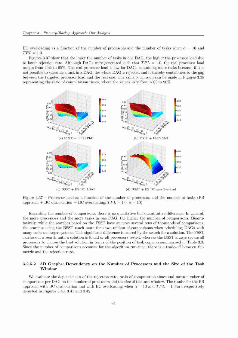
Chapter 3 – Primary/Backup Approach: Our Analysis

BC overloading as a function of the number of processors and the number of tasks when α = 10 andT P L = 1.0.

Figures 3.37 show that the lower the number of tasks in one DAG, the higher the processor load dueto lower rejection rate. Although DAGs were generated such that T P L = 1.0, the real processor loadranges from 40% to 65%. The real processor load is low for DAGs containing more tasks because, if it isnot possible to schedule a task in a DAG, the whole DAG is rejected and it thereby contributes to the gapbetween the targeted processor load and the real one. The same conclusion can be made in Figures 3.38representing the ratio of computation times, where the values vary from 50% to 90%.

Numb

er of tasks

020

4060

80100

Number of processors 510152025

Processor load

0.400.450.500.550.600.65

0.40

0.45

0.50

0.55

0.60

(a) FSST + FFSS PbP

Numb

er of tasks

020

4060

80100

Number of processors 510152025

Processor load

0.400.450.500.550.600.650.70

0.40

0.45

0.50

0.55

0.60

(b) FSST + FFSS SbS

Numb

er of tasks

020

4060

80100

Number of processors 510152025

Processor load

0.400.450.500.550.60

0.65

0.40

0.45

0.50

0.55

(c) BSST + ES BC ASAP

Numb

er of tasks

020

4060

80100

Number of processors 510152025

Processor load

0.450.500.550.60

0.65

0.45

0.50

0.55

0.60

0.65

(d) BSST + ES BC maxOverload

Figure 3.37 – Processor load as a function of the number of processors and the number of tasks (PBapproach + BC deallocation + BC overloading; T P L = 1.0; α = 10)

Regarding the number of comparisons, there is no qualitative but quantitative difference. In general,the more processors and the more tasks in one DAG, the higher the number of comparisons. Quanti-tatively, while the searches based on the FSST have at most several tens of thousands of comparisons,the searches using the BSST reach more than two million of comparisons when scheduling DAGs withmany tasks on larger systems. This significant difference is caused by the search for a solution. The FSSTcarries out a search until a solution is found or all processors tested, whereas the BSST always scours allprocessors to choose the best solution in terms of the position of task copy, as summarised in Table 3.3.Since the number of comparisons accounts for the algorithm run-time, there is a trade-off between thismetric and the rejection rate.

3.2.5.2 3D Graphs: Dependency on the Number of Processors and the Size of the TaskWindow

We evaluate the dependencies of the rejection rate, ratio of computation times and mean number ofcomparisons per DAG on the number of processors and the size of the task window. The results for the PBapproach with BC deallocation and with BC overloading when α = 10 and T P L = 1.0 are respectivelydepicted in Figures 3.40, 3.41 and 3.42.

84

3.2. Dependent Tasks

Numb

er of tasks

020

4060

80100

Number of processors 510152025

Ratio of computation tim

es

0.5

0.6

0.7

0.8

0.5

0.6

0.7

(a) FSST + FFSS PbP

Numb

er of tasks

020

4060

80100

Number of processors 510152025

Ratio of computation tim

es

0.5

0.6

0.7

0.8

0.500.550.600.650.700.75

(b) FSST + FFSS SbS

Numb

er of tasks

020

4060

80100

Number of processors 510152025

Ratio of computation tim

es

0.450.500.550.600.650.700.750.80

0.50

0.55

0.60

0.65

0.70

(c) BSST + ES BC ASAP

Numb

er of tasks

020

4060

80100

Number of processors 510152025

Ratio of computation tim

es

0.5

0.6

0.7

0.8

0.9

0.5

0.6

0.7

0.8

(d) BSST + ES BC maxOverload

Figure 3.38 – Ratio of computation times as a function of the number of processors and the number oftasks (PB approach + BC deallocation + BC overloading; T P L = 1.0; α = 10)

Number of tasks

020

406080100

Number of processors 510152025

Mean com

p. per DAG 5×103104

1.5×1042×1042.5×1043×1043.5×104

5.0×103

1.0×104

1.5×104

2.0×104

(a) FSST + FFSS PbP

Number of tasks

020

406080100

Number of processors 510152025

Mean com

p. per DAG 2.5×1045×1047.5×104105

1.25×1051.5×1051.75×1052×105

2.5×104

5.0×104

7.5×104

1.0×105

(b) FSST + FFSS SbS

Number of tasks

020

406080100

Number of processors 510152025

Mean com

p. per DAG

2×105

4×105

6×105

8×105

106

2.0×105

4.0×105

6.0×105

(c) BSST + ES BC ASAP

Number of tasks

020

406080100

Number of processors 510152025

Mean com

p. per DAG 5×105106

1.5×1062×1062.5×1063×1063.5×106

5.0×105

1.0×106

1.5×106

2.0×106

(d) BSST + ES BC maxOverload

Figure 3.39 – Mean number of comparisons per DAG (all DAGs considered) as a function of the numberof processors and the number of tasks (PB approach + BC deallocation + BC overloading; T P L = 1.0;α = 10)

85

Chapter 3 – Primary/Backup Approach: Our Analysis

We observe that the lower the number of processors and the smaller the task window, (i) the higher therejection rate, (ii) the lower the ratio of computation times, and (iii) the lower the number of comparisons.The dependency on the number of processors has already been explained in the preceding section. Asregards the dependency on the size of the task window, the larger the task window, the higher probabilityto find a slot large enough to accommodate a task copy. This yields better system performances (lowerrejection rate and higher ratio of computation times) but at the cost of higher algorithm run-time (highernumber of comparisons). Again, the BSST + ES BC maxOverload has lower task rejection (when thetask window is large and DAGs have more tasks) than other studied techniques.

α

24

6810

Number of processors 510152025

Rejection rate

0.4

0.5

0.6

0.7

0.4

0.5

0.6

(a) FSST + FFSS PbP

α

24

6810

Number of processors 510152025

Rejection rate

0.350.400.450.500.550.600.650.70

0.40

0.45

0.50

0.55

0.60

(b) FSST + FFSS SbS

α

24

6810

Number of processors 510152025

Rejection rate

0.4

0.5

0.6

0.7

0.40

0.45

0.50

0.55

0.60

(c) BSST + ES BC ASAP

α

24

6810

Number of processors 510152025

Rejection rate

0.20.30.40.50.60.7

0.2

0.3

0.4

0.5

0.6

(d) BSST + ES BC maxOverload

Figure 3.40 – Rejection rate as a function of the number of processors and the size of the task window(PB approach + BC deallocation + BC overloading; T P L = 1.0; α = 10)

3.2.5.3 2D Graphs: Dependency on the Number of Processors

In the preceding sections, we analysed the dependency of the studied metrics in three dimensions.The merit of this visualisation is that it is possible to easier apprehend the evolution of metrics on twoparameters at the same time. This is convenient especially for dependent tasks having several parameters,such as the number of tasks in one DAG or the size of the task window. Nonetheless, the 3D representationis not well appropriate to compare different techniques. This is the reason why we analyse also twodimensional graphical representations.

The results of the rejection rate for the PB approach with BC deallocation and with BC overloadingas a function of the number of processors when α = 10 are represented in Figures 3.43 and 3.44 forT P L = 0.5 and T P L = 1.0, respectively. The value of the targeted processor load has a significantimpact on the rejection rate: the higher its value, the higher the rejection rate. When T P L = 0.5, alltechniques have almost similar performances although the FSST + FFSS SbS and BSST + ES BCmaxOverload perform slightly better for DAGs consisting of only several tasks. For T P L = 1.0, whenthere are less than 5 processors, there is no difference among techniques but starting with 6 processorsthe gap between the BSST + ES BC maxOverload and other techniques gets larger because the BSST

86

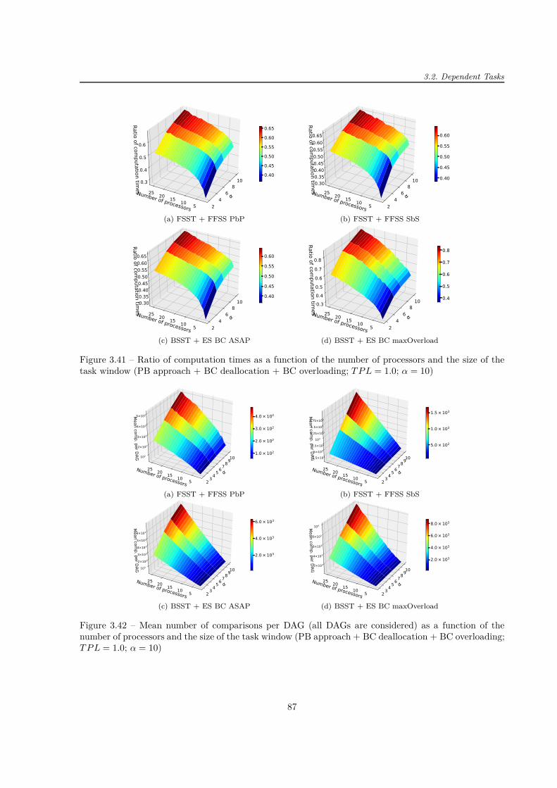
3.2. Dependent Tasks

α

24

6810

Number of processors 510152025

Ratio of computation tim

es

0.3

0.4

0.5

0.6

0.400.450.500.550.600.65

(a) FSST + FFSS PbP

α

24

6810

Number of processors 510152025

Ratio of computation tim

es

0.300.350.400.450.500.550.600.65

0.40

0.45

0.50

0.55

0.60

(b) FSST + FFSS SbS

α

24

6810

Number of processors 510152025

Ratio of computation tim

es

0.300.350.400.450.500.550.600.65

0.40

0.45

0.50

0.55

0.60

(c) BSST + ES BC ASAP

α

24

6810

Number of processors 510152025

Ratio of computation tim

es

0.30.40.50.60.70.8

0.4

0.5

0.6

0.7

0.8

(d) BSST + ES BC maxOverload

Figure 3.41 – Ratio of computation times as a function of the number of processors and the size of thetask window (PB approach + BC deallocation + BC overloading; T P L = 1.0; α = 10)

α

2345

678910

Number of processors 510152025

Mean com

p. per DAG 102

2×102

3×102

4×102

5×102

1.0×102

2.0×102

3.0×102

4.0×102

(a) FSST + FFSS PbP

α

2345

678910

Number of processors 510152025

Mean com

p. per DAG 2.5×1025×1027.5×102103

1.25×1031.5×1031.75×103

5.0×102

1.0×103

1.5×103

(b) FSST + FFSS SbS

α

2345

678910

Number of processors 510152025

Mean com

p. per DAG 1032×1033×1034×1035×1036×103

2.0×103

4.0×103

6.0×103

(c) BSST + ES BC ASAP

α

2345

678910

Number of processors 510152025

Mean com

p. per DAG 2×103

4×103

6×103

8×103

104

2.0×103

4.0×103

6.0×103

8.0×103

(d) BSST + ES BC maxOverload

Figure 3.42 – Mean number of comparisons per DAG (all DAGs are considered) as a function of thenumber of processors and the size of the task window (PB approach + BC deallocation + BC overloading;T P L = 1.0; α = 10)

87

Chapter 3 – Primary/Backup Approach: Our Analysis

+ ES BC maxOverload rejects less tasks than other techniques. This gap is also noticeable for the ratioof computation times represented in Figure 3.45.

2 4 6 8 10 12 14 16 18 20 22 24Number of processors (TPL = 0.5)

0.000

0.025

0.050

0.075

0.100

0.125

0.150

Rejection rate

(a) 10 tasks

2 4 6 8 10 12 14 16 18 20 22 24Number of processors (TPL = 0.5)

0.05

0.10

0.15

0.20

0.25

0.30

Rejection rate

(b) 100 tasks

Figure 3.43 – Rejection rate as a function of the number of processors (PB approach + BC deallocation+ BC overloading; T P L = 0.5; α = 10)

2 4 6 8 10 12 14 16 18 20 22 24Number of processors (TPL = 1.0)

0.15

0.20

0.25

0.30

0.35

0.40

0.45

0.50

0.55

Rejection rate

(a) 10 tasks

2 4 6 8 10 12 14 16 18 20 22 24Number of processors (TPL = 1.0)

0.20

0.25

0.30

0.35

0.40

0.45

0.50

0.55

Rejection rate

(b) 100 tasks

Figure 3.44 – Rejection rate as a function of the number of processors (PB approach + BC deallocation+ BC overloading; T P L = 1.0; α = 10)

2 4 6 8 10 12 14 16 18 20 22 24Number of processors (TPL = 1.0)

0.50

0.55

0.60

0.65

0.70

0.75

0.80

0.85

Ratio

of c

ompu

tatio

n tim

es

(a) 10 tasks

2 4 6 8 10 12 14 16 18 20 22 24Number of processors (TPL = 1.0)

0.45

0.50

0.55

0.60

0.65

0.70

0.75

0.80

Ratio

of c

ompu

tatio

n tim

es

(b) 100 tasks

Figure 3.45 – Ratio of computation times as a function of the number of processors (PB approach + BCdeallocation + BC overloading; T P L = 1.0; α = 10)

Regarding the algorithm run-time, the mean number of comparisons per DAG composed of 10 and100 tasks are depicted in Figures 3.46. The BSST requires significantly more comparisons than the FSSTfor it always tests all possibilities on all processors. The BSST + ES BC ASAP has less comparisonsthan the BSST + ES BC maxOverload and the FFSS PbP is quicker than the FFSS SbS. We thereforeconclude that, when scheduling dependent tasks, it is better to test all free slots on one processor beforetrying the next one. The analysis of the maximum number of comparisons per DAG shows that the trend

88

3.2. Dependent Tasks

of curves is similar to the ones plotted in Figures 3.46 but their values are approximately four timeshigher.

2 4 6 8 10 12 14 16 18 20 22 24Number of processors (TPL = 1.0)

0

2×103

4×103

6×103

8×103

104

Mea

n co

mpa

rison

s per

DAG

(all

DAGs

con

sider

ed)

(a) 10 tasks

2 4 6 8 10 12 14 16 18 20 22 24Number of processors (TPL = 1.0)

0

5×105106

1.5×1062×106

2.5×1063×106

3.5×106

Mean comparisons p

er DAG

(all DA

Gs consid

ered)

(b) 100 tasks

Figure 3.46 – Mean number of comparisons per DAG (all DAGs are considered) as a function of thenumber of processors (PB approach + BC deallocation + BC overloading; T P L = 1.0; α = 10)

3.2.5.4 2D Graphs: Dependency on the Number of Tasks

In this section, we evaluate the dependencies of the rejection rate and the mean number of comparisonsper DAG on the number of tasks. The results for the PB approach with BC deallocation and withBC overloading when α = 10 and T P L = 1.0 are respectively depicted in Figures 3.47 and 3.48 forP ∈ 4, 14, 24.

In general, when DAGs contain more tasks, both the rejection rate and the number of comparisonsincrease and the gap between the BSST and FSST gets larger. The BSST + ES BC maxOverload achieveslower rejection rate than other techniques but at the cost of higher number of comparisons.

2 10 20 30 40 50 100Number of DAGs (TPL = 1.0)

0.325

0.350

0.375

0.400

0.425

0.450

0.475

0.500

0.525

Rejection rate

FSST + FFSS PbPFSST + FFSS SbSBSST + ES BC ASAPBSST + ES BC maxOverload

(a) P = 4

2 10 20 30 40 50 100Number of DAGs (TPL = 1.0)

0.20

0.25

0.30

0.35

0.40

0.45

0.50

Reje

ctio

n rate

FSST + FFSS PbPFSST + FFSS SbSBSST + ES BC ASAPBSST + ES BC maxOverload

(b) P = 14

2 10 20 30 40 50 100Number of DAGs (TPL = 1.0)

0.10

0.15

0.20

0.25

0.30

0.35

0.40

0.45

Reje

ctio

n rate

FSST + FFSS PbPFSST + FFSS SbSBSST + ES BC ASAPBSST + ES BC maxOverload

(c) P = 24

Figure 3.47 – Rejection rate as a function of the number of tasks (PB approach + BC deallocation + BCoverloading; T P L = 1.0; α = 10)

3.2.5.5 2D Graphs: Dependency on the Size of the Task Window

We assess the dependencies of the rejection rate and the mean number of comparisons per DAG on thesize of the task window. The results for the PB approach with BC deallocation and with BC overloadingwhen α = 10, P = 14 and T P L = 1.0 are respectively depicted in Figures 3.49 and 3.50 for 10 and 100tasks in one DAG.

When the size of the task window increases, i.e. when the multiple of the computation times is greater,the lower the rejection rate, the higher the number of comparisons and the larger the gap between theBSST and the FSST due to more possibilities tested.

89

Chapter 3 – Primary/Backup Approach: Our Analysis

2 10 20 30 40 50 100Number of DAGs (TPL = 1.0)

0

2.5×1045×104

7.5×104105

1.25×1051.5×105

1.75×105

Mean compa

rison

s per DAG

(all DA

Gs con

sidered

)

FSST + FFSS PbPFSST + FFSS SbSBSST + ES BC ASAPBSST + ES BC maxOverload

(a) P = 4

2 10 20 30 40 50 100Number of DAGs (TPL = 1.0)

0

2.5×105

5×105

7.5×105

106

1.25×106

1.5×106

1.75×106

Mean compa

rison

s per DAG

(all DA

Gs con

sidered

)

FSST + FFSS PbPFSST + FFSS SbSBSST + ES BC ASAPBSST + ES BC maxOverload

(b) P = 14

2 10 20 30 40 50 100Number of DAGs (TPL = 1.0)

0

5×105106

1.5×1062×106

2.5×1063×106

3.5×106

Mean compa

rison

s per DAG

(all DA

Gs con

sidered

)

FSST + FFSS PbPFSST + FFSS SbSBSST + ES BC ASAPBSST + ES BC maxOverload

(c) P = 24

Figure 3.48 – Mean number of comparisons per DAG (all DAGs are considered) as a function of thenumber of tasks (PB approach + BC deallocation + BC overloading; T P L = 1.0; α = 10)

2 3 4 5 6 7 8 9 10α (TPL = 1.0)

0.25

0.30

0.35

0.40

0.45

0.50

Rejection rate

(a) 10 tasks

2 3 4 5 6 7 8 9 10α (TPL = 1.0)

0.30

0.35

0.40

0.45

0.50

0.55

Rejection rate

(b) 100 tasks

Figure 3.49 – Rejection rate as a function of the size of the task window (PB approach + BC deallocation+ BC overloading; T P L = 1.0; P = 14; α = 10)

2 3 4 5 6 7 8 9 10α (TPL = 1.0)

0

103

2×103

3×103

4×103

5×103

Mea

n co

mpa

rison

s per

DAG

(all

DAGs

con

sider

ed)

(a) 10 tasks

2 3 4 5 6 7 8 9 10α (TPL = 1.0)

0

2.5×105

5×105

7.5×105

106

1.25×106

1.5×106

1.75×106

Mea

n co

mpa

rison

s per

DAG

(all

DAGs

con

sider

ed)

(b) 100 tasks

Figure 3.50 – Mean number of comparisons per DAG (all DAGs are considered) as a function of the sizeof the task window (PB approach + BC deallocation + BC overloading; T P L = 1.0; P = 14; α = 10)

3.2.5.6 Comparison with Already Published Results

After presenting our results, we draw a comparison with results already published in papers. TheBSST + ES BC ASAP is close to the online method in [155], which is an update of an offline methodpresented in [121]. The BSST + ES BC maxOverload is similar to another method published in [155].

The difference between our implementation of the BSST and the one in [155] is that while a primarycopy can start before a backup copy of their predecessors (but after their respective primary copies) in[155], in our experimental framework all task copies of predecessors must be finished before a successortask can start its execution. The reason for doing so in our implementation is to reduce the schedulingconstraints and consequently avoid longer algorithm time.

Table 3.7 compares two aforementioned methods with our results for a 16-processor system. The maindifference is in the dependency on the processor load. In fact, when the targeted processor load increases,the rejection rate in [155] remains almost constant while our rejection rate increases, which seems logical

90

3.2. Dependent Tasks

because the higher the targeted processor load, the lower the probability to schedule all tasks. As regardsthe dependency on the task deadline, both results show that the tighter the deadline, the higher therejection rate. The obtained values are different, which is probably caused by the different definitions ofthe task window. While a task window is defined as a multiple α ∈ [2; 5] of the task computation time inour simulations, a task window in [155] is determined as η · 2texe

5.5 , where η ∈ [0.2; 0.3], texe is the executiontime of the DAG containing the task and 5.5 is the mean processing speed.

Table 3.7 – Comparison of our results with the ones from [155] for the 16-processor system

[155] Our implementation

BSST + ES BC max overloading

When TPLincreases

Rejection rate remains almost the same(mean of 20, 40, 60, 80, 100 tasks: 13% for

T P L ∈ [0.05; 0.8])

Rejection rate increases (10 tasks: 0% forT P L = 0.5 and 22% for T P L = 1.0; 100 tasks:

7% for T P L = 0.5 and 25% for T P L = 1.0)

Whendeadline is

tighter

Rejection rate increases (mean of 20, 40, 60,80, 100 tasks: 39% for the smallest studied taskwindow and 3% for the largest studied window)

Rejection rate increases (10 tasks: 47% forthe smallest studied task window (α = 2) and23% for the largest studied window (α = 10);100 tasks: 44% for α = 2 and 26% for α = 10)

BSST +ES BC ASAP

When TPLincreases

Rejection rate remains almost the same(mean of 20, 40, 60, 80, 100 tasks: 15% for

T P L ∈ [0.05; 0.8])

Rejection rate increases (10 tasks: 0% forT P L = 0.5 and 22% for T P L = 1.0; 100 tasks:

7% for T P L = 0.5 and 25% for T P L = 1.0)

Whendeadline is

tighter

Rejection rate increases (mean of 20, 40, 60,80, 100 tasks: 40% for the smallest studied taskwindow and 3% for the largest studied window)

Rejection rate increases (10 tasks: 50% forthe smallest studied task window (α = 2) and39% for the largest studied window (α = 10);100 tasks: 55% for α = 2 and 49% for α = 10)

3.2.5.7 Simulations with Fault Injection

Before presenting the results of different metrics, we carry out a fault analysis. Figures 3.51, 3.52,3.53 and 3.54 depict the total number of faults against the number of processors, while the total numberis the sum of the faults without impact, faults impacting simple tasks and faults impacting double tasks.These figures show such numbers for the PB approach with BC deallocation and with BC overloadingwhen scheduling DAGs consisting of 10, 20, 50 and 100 tasks using the BSST + ES BC maxOverload.The fault rates injected per processor and represented in figures equal 1 ·10−5 fault/ms (corresponding tothe worst estimated fault rate in a harsh environment [118]), 4 ·10−4 fault/ms (corresponding to the limitof the assumption of only one fault in the system at the same time for a 25-processor system), 1 · 10−3

fault/ms and 1 · 10−2 fault/ms.

2 4 6 8 10 12 14 16 18 20 22 24Number of processors

0.0

0.1

0.2

0.3

0.4

0.5

0.6

0.7

0.8

Number

Faults without impactFaults impacting PCFaults impacting BC

(a) 10 tasks

2 4 6 8 10 12 14 16 18 20 22 24Number of processors

0.0

0.2

0.4

0.6

0.8

1.0

1.2

1.4

Numbe

r

Faults without impactFaults impacting PCFaults impacting BC

(b) 20 tasks

2 4 6 8 10 12 14 16 18 20 22 24Number of processors

0.0

0.5

1.0

1.5

2.0

2.5

3.0

3.5

4.0

Number

Faults without impactFaults impacting PCFaults impacting BC

(c) 50 tasks

2 4 6 8 10 12 14 16 18 20 22 24Number of processors

0

1

2

3

4

5

6

7

8

Number

Faults without impactFaults impacting PCFaults impacting BC

(d) 100 tasks

Figure 3.51 – Total number of faults (injected with the fault rate of 1 · 10−5 fault/ms) against thenumber of processors (PB approach + BC deallocation + BC overloading; BSST + ES BC maxOverload;T P L = 1.0; α = 10)

Although results only for the BSST + ES BC maxOverload are shown, other approaches achievesimilar values, except when the fault rate is higher than 1 · 10−3 fault/ms. In such a case, the BSST +

91

Chapter 3 – Primary/Backup Approach: Our Analysis

2 4 6 8 10 12 14 16 18 20 22 24Number of processors

0

5

10

15

20

25

Numbe

r Faults without impactFaults impacting PCFaults impacting BC

(a) 10 tasks

2 4 6 8 10 12 14 16 18 20 22 24Number of processors

0

10

20

30

40

50

Numbe

r Faults without impactFaults impacting PCFaults impacting BC

(b) 20 tasks

2 4 6 8 10 12 14 16 18 20 22 24Number of processors

0

20

40

60

80

100

Numbe

r Faults without impactFaults impacting PCFaults impacting BC

(c) 50 tasks

2 4 6 8 10 12 14 16 18 20 22 24Number of processors

0

50

100

150

200

Numbe

r Faults without impactFaults impacting PCFaults impacting BC

(d) 100 tasks

Figure 3.52 – Total number of faults (injected with the fault rate of 4 · 10−4 fault/ms) against thenumber of processors (PB approach + BC deallocation + BC overloading; BSST + ES BC maxOverload;T P L = 1.0; α = 10)

2 4 6 8 10 12 14 16 18 20 22 24Number of processors

0

10

20

30

40

50

60

Numbe

r Faults without impactFaults impacting PCFaults impacting BC

(a) 10 tasks

2 4 6 8 10 12 14 16 18 20 22 24Number of processors

0

20

40

60

80

100

Numbe

r Faults without impactFaults impacting PCFaults impacting BC

(b) 20 tasks

2 4 6 8 10 12 14 16 18 20 22 24Number of processors

0

50

100

150

200

250Nu

mbe

r Faults without impactFaults impacting PCFaults impacting BC

(c) 50 tasks

2 4 6 8 10 12 14 16 18 20 22 24Number of processors

0

100

200

300

400

500

Numbe

r

Faults without impactFaults impacting PCFaults impacting BC

(d) 100 tasks

Figure 3.53 – Total number of faults (injected with the fault rate of 1 · 10−3 fault/ms) against thenumber of processors (PB approach + BC deallocation + BC overloading; BSST + ES BC maxOverload;T P L = 1.0; α = 10)

2 4 6 8 10 12 14 16 18 20 22 24Number of processors

0

100

200

300

400

500

Numbe

r

Faults without impactFaults impacting PCFaults impacting BC

(a) 10 tasks

2 4 6 8 10 12 14 16 18 20 22 24Number of processors

0

200

400

600

800

1000

Numbe

r

Faults without impactFaults impacting PCFaults impacting BC

(b) 20 tasks

2 4 6 8 10 12 14 16 18 20 22 24Number of processors

0

500

1000

1500

2000

2500

Numbe

r

Faults without impactFaults impacting PCFaults impacting BC

(c) 50 tasks

2 4 6 8 10 12 14 16 18 20 22 24Number of processors

0

1000

2000

3000

4000

5000

Numbe

r

Faults without impactFaults impacting PCFaults impacting BC

(d) 100 tasks

Figure 3.54 – Total number of faults (injected with the fault rate of 1 · 10−2 fault/ms) against thenumber of processors (PB approach + BC deallocation + BC overloading; BSST + ES BC maxOverload;T P L = 1.0; α = 10)

ES BC maxOverload has higher number of impacted copies due to lower rejection rate than the FSST +FFSS SbS and the FSST + FFSS PbP). The BSST + ES BC ASAP is not evaluated because it performsas the FSST but exhibits higher number of comparisons.

The number of impacted copies increases when a DAG contains more tasks and if faults occur morefrequently. Even for the fault rate 1 · 10−3 fault/ms, which is higher by two orders of magnitude than theworst estimated fault rate, the number of impacted faults is low, except for DAGs containing 100 tasks.This is partially due to the non-negligible rejection rate and therefore lower processor load.

Next, we analyse the rejection rate, the system throughout, the processor load and the mean numberof comparisons per DAG for the PB approach with BC deallocation and with BC overloading as a functionof the number of processors when α = 10 and T P L = 1.0. These metrics are respectively depicted inFigures 3.55, 3.57, 3.59 and 3.60 for the FSST + FFSS PbP, the FSST + FFSS SbS and the BSST + ES

92

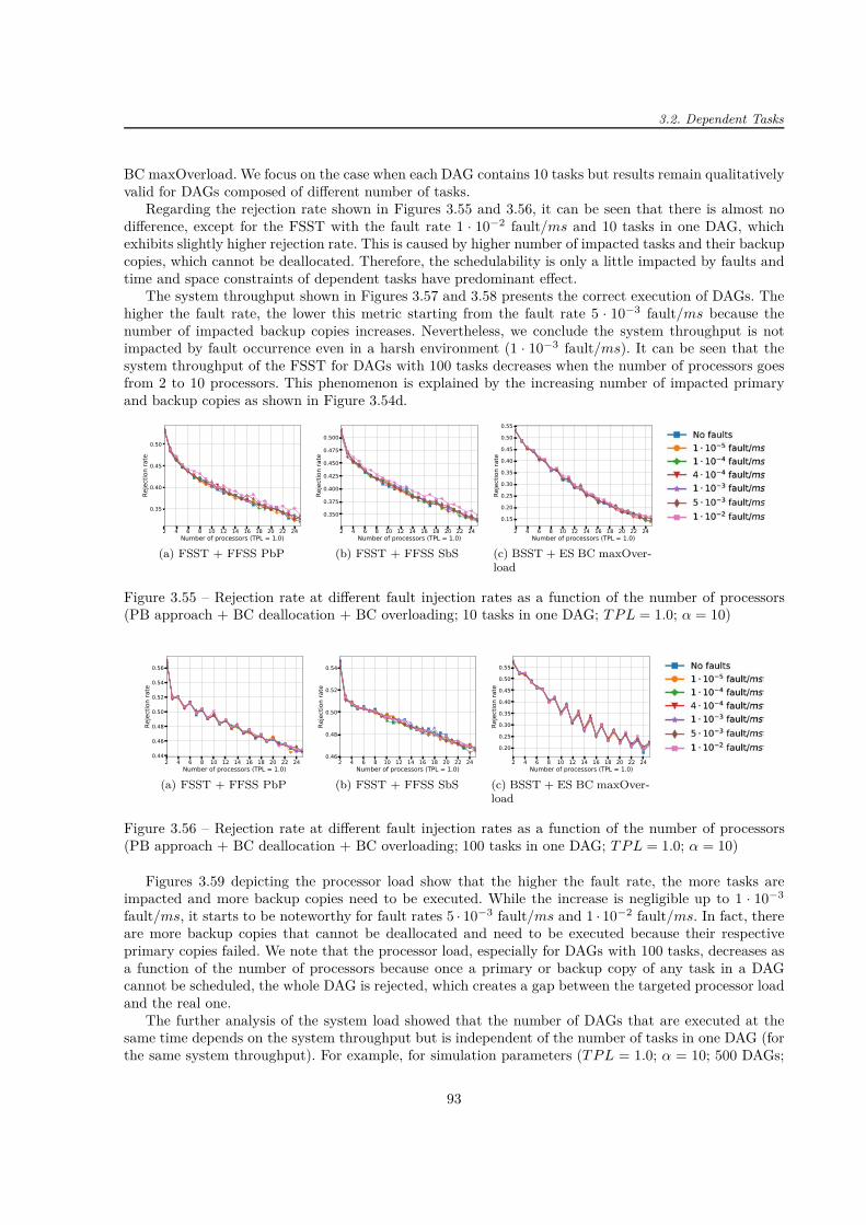
3.2. Dependent Tasks

BC maxOverload. We focus on the case when each DAG contains 10 tasks but results remain qualitativelyvalid for DAGs composed of different number of tasks.

Regarding the rejection rate shown in Figures 3.55 and 3.56, it can be seen that there is almost nodifference, except for the FSST with the fault rate 1 · 10−2 fault/ms and 10 tasks in one DAG, whichexhibits slightly higher rejection rate. This is caused by higher number of impacted tasks and their backupcopies, which cannot be deallocated. Therefore, the schedulability is only a little impacted by faults andtime and space constraints of dependent tasks have predominant effect.

The system throughput shown in Figures 3.57 and 3.58 presents the correct execution of DAGs. Thehigher the fault rate, the lower this metric starting from the fault rate 5 · 10−3 fault/ms because thenumber of impacted backup copies increases. Nevertheless, we conclude the system throughput is notimpacted by fault occurrence even in a harsh environment (1 · 10−3 fault/ms). It can be seen that thesystem throughput of the FSST for DAGs with 100 tasks decreases when the number of processors goesfrom 2 to 10 processors. This phenomenon is explained by the increasing number of impacted primaryand backup copies as shown in Figure 3.54d.

2 4 6 8 10 12 14 16 18 20 22 24Number of processors (TPL = 1.0)

0.35

0.40

0.45

0.50

Rejection rate

(a) FSST + FFSS PbP

2 4 6 8 10 12 14 16 18 20 22 24Number of processors (TPL = 1.0)

0.350

0.375

0.400

0.425

0.450

0.475

0.500

Reje

ctio

n ra

te

(b) FSST + FFSS SbS

2 4 6 8 10 12 14 16 18 20 22 24Number of processors (TPL = 1.0)

0.15

0.20

0.25

0.30

0.35

0.40

0.45

0.50

0.55

Rejection rate

(c) BSST + ES BC maxOver-load

Figure 3.55 – Rejection rate at different fault injection rates as a function of the number of processors(PB approach + BC deallocation + BC overloading; 10 tasks in one DAG; T P L = 1.0; α = 10)

2 4 6 8 10 12 14 16 18 20 22 24Number of processors (TPL = 1.0)

0.44

0.46

0.48

0.50

0.52

0.54

0.56

Rejection rate

(a) FSST + FFSS PbP

2 4 6 8 10 12 14 16 18 20 22 24Number of processors (TPL = 1.0)

0.46

0.48

0.50

0.52

0.54

Rejection rate

(b) FSST + FFSS SbS

2 4 6 8 10 12 14 16 18 20 22 24Number of processors (TPL = 1.0)

0.20

0.25

0.30

0.35

0.40

0.45

0.50

0.55

Rejection rate

(c) BSST + ES BC maxOver-load

Figure 3.56 – Rejection rate at different fault injection rates as a function of the number of processors(PB approach + BC deallocation + BC overloading; 100 tasks in one DAG; T P L = 1.0; α = 10)

Figures 3.59 depicting the processor load show that the higher the fault rate, the more tasks areimpacted and more backup copies need to be executed. While the increase is negligible up to 1 · 10−3

fault/ms, it starts to be noteworthy for fault rates 5 · 10−3 fault/ms and 1 · 10−2 fault/ms. In fact, thereare more backup copies that cannot be deallocated and need to be executed because their respectiveprimary copies failed. We note that the processor load, especially for DAGs with 100 tasks, decreases asa function of the number of processors because once a primary or backup copy of any task in a DAGcannot be scheduled, the whole DAG is rejected, which creates a gap between the targeted processor loadand the real one.

The further analysis of the system load showed that the number of DAGs that are executed at thesame time depends on the system throughput but is independent of the number of tasks in one DAG (forthe same system throughput). For example, for simulation parameters (T P L = 1.0; α = 10; 500 DAGs;

93

Chapter 3 – Primary/Backup Approach: Our Analysis

2 4 6 8 10 12 14 16 18 20 22 24Number of processors (TPL = 1.0)

250

300

350

400

450

500

System

throug

hput

(a) FSST + FFSS PbP

2 4 6 8 10 12 14 16 18 20 22 24Number of processors (TPL = 1.0)

250

300

350

400

450

500

System

throug

hput

(b) FSST + FFSS SbS

2 4 6 8 10 12 14 16 18 20 22 24Number of processors (TPL = 1.0)

250

300

350

400

450

500

System

throug

hput

(c) BSST + ES BC maxOver-load

Figure 3.57 – System throughout at different fault injection rates as a function of the number of processors(PB approach + BC deallocation + BC overloading ; 10 tasks in one DAG; T P L = 1.0; α = 10)

2 4 6 8 10 12 14 16 18 20 22 24Number of processors (TPL = 1.0)

100

150

200

250

300

350

400

450

500

System

throug

hput

(a) FSST + FFSS PbP

2 4 6 8 10 12 14 16 18 20 22 24Number of processors (TPL = 1.0)

100

150

200

250

300

350

400

450

500

System

throug

hput

(b) FSST + FFSS SbS

2 4 6 8 10 12 14 16 18 20 22 24Number of processors (TPL = 1.0)

150

200

250

300

350

400

450

500

System

throug

hput

(c) BSST + ES BC maxOver-load

Figure 3.58 – System throughout at different fault injection rates as a function of the number of processors(PB approach + BC deallocation + BC overloading; 100 tasks in one DAG; T P L = 1.0; α = 10)

FSST + FFSS SbS; no fault injected), they are approximately 2 DAGs for 4-processor system, 6 DAGsfor 14-processor system and 9 DAGs for 25-processor system.

2 4 6 8 10 12 14 16 18 20 22 24Number of processors (TPL = 1.0)

0.48

0.50

0.52

0.54

0.56

0.58

0.60

0.62

Proc

essor loa

d

(a) FSST + FFSS PbP

2 4 6 8 10 12 14 16 18 20 22 24Number of processors (TPL = 1.0)

0.48

0.50

0.52

0.54

0.56

0.58

0.60

0.62

0.64

Proc

essor loa

d

(b) FSST + FFSS SbS

2 4 6 8 10 12 14 16 18 20 22 24Number of processors (TPL = 1.0)

0.50

0.55

0.60

0.65

0.70

Proc

essor loa

d

(c) BSST + ES BC maxOver-load

Figure 3.59 – Processor load at different fault injection rates as a function of the number of processors(PB approach + BC deallocation + BC overloading; 10 tasks in one DAG; T P L = 1.0; α = 10)

Regarding the number of comparisons, all studied fault rates, except 1 · 10−2 fault/ms for FSST,require similar number of comparisons. Less comparisons for the fault rate of 1 · 10−2 fault/ms is causedby higher rejection rate. Actually, although before finding out that a primary or backup copy of any taskin a DAG cannot be scheduled, all possibilities are tested, the task causing the rejection can be anywherein the DAG, which lowers the mean number of comparisons per DAG.

The thorough analysis was also carried out for the same simulation parameters when T P L = 0.5.The values of the studied metrics were proportional to a system with lower targeted processor load, asit can be seen for the rejection rate of different methods when T P L = 0.5 (Figures 3.35) and whenT P L = 1.0 (Figures 3.36). Nonetheless, the algorithm performances do not change, which means thatthe schedulability is only a little impacted by faults and that task dependencies have predominant effect.

94

3.3. Summary

2 4 6 8 10 12 14 16 18 20 22 24Number of processors (TPL = 1.0)

102

2×102

3×102

4×102

5×102

Mean comparisons p

er DAG

(all DA

Gs consid

ered)

(a) FSST + FFSS PbP

2 4 6 8 10 12 14 16 18 20 22 24Number of processors (TPL = 1.0)

2.5×1025×102

7.5×102103

1.25×1031.5×103

1.75×1032×103

Mea

n compa

rison

s per DAG

(all DA

Gs con

sidered

)

(b) FSST + FFSS SbS

2 4 6 8 10 12 14 16 18 20 22 24Number of processors (TPL = 1.0)

0

2×103

4×103

6×103

8×103

104

Mea

n co

mpa

rison

s per

DAG

(all

DAGs

con

sider

ed)

(c) BSST + ES BC maxOver-load

Figure 3.60 – Mean number of comparisons per one DAG at different fault injection rates as a functionof the number of processors (PB approach + BC deallocation + BC overloading; 10 tasks in one DAG;T P L = 1.0; α = 10)

3.3 Summary

This chapter presents our achievements related to the primary/backup approach for both independentand dependent tasks. They show various aspects of fault tolerant scheduling of aperiodic tasks based onthe primary/backup approach.

The next ten paragraphs enumerate the main results of the scheduling of the independent tasks.First, the results of the PB approach by itself and the one with BC overloading show that the BC

overloading facilitates the reduction of the rejection rate (for example 14% for a 14-processor systemwith T P L = 1.0). When the BC deallocation is then put into practice, the improvement is even morenoteworthy. For instance for the 14-processor system and T P L = 1.0, the gain is about 75% compared tothe baseline PB approach and no matter whether the BC overloading is implemented or not. Moreover,it was shown that the BC overloading and the BC deallocation work well together.

Second, the active PB approach was evaluated. It was demonstrated that it allows systems to deal withtasks having tight deadline and it therefore reduces the rejection rate. For example, for the 14-processorsystem and T P L = 1.0, there is a drop of about 17% for both the PB approach with BC deallocationand with or without BC overloading.

Third, three different processor allocation policies were studied: the exhaustive search (ES), the firstfound solution search - processor by processor (FFSS PbP) and the first found solution search - slot by slot(FFSS SbS). On the one hand, it was found that the ES achieves the lowest rejection rate compared tothe other two searches but it has the highest values for the maximum and mean numbers of comparisonsper task. On the other hand, the FFSS SbS performs better than the FFSS PbP. While its rejection rateis higher by about 12% compared to the ES (14 processors), the maximum number of comparisons issignificantly lower than the one for the FFSS PbP (29% for the 14-processor system) and the ES (about41% for the 14-processor system). Moreover, the mean number of comparisons is only slightly dependenton the number of processors, which is advantageous to systems with many resources. When comparingthe results to the optimal solution, the algorithm based on the FFSS SbS is 2-competitive.

Fourth, two scheduling search techniques were analysed: the free slot search technique (FSST) andthe boundary schedule search technique (BSST). The BSST + ES achieves similar rejection rate as theFSST + ES and the number of comparisons of the BSST is significantly higher than the one of the FSST(more than twice). The BSST is consequently not a convenient scheduling search technique to reduce thealgorithm run-time.

Fifth, the overheads of the algorithm based on the primary/backup approach were also analysed.Since this approach reserves slots for its primary and backup copies (even if the BC deallocation is putinto practice), the higher the number of processors, the more comparisons to find slots for both copiesand consequently the wider the gap in the number of comparisons between fault tolerant and non-faulttolerant systems. It was also shown that the more processors, the narrower the gap in the rejection ratebetween fault tolerant system using the primary/backup approach and non-fault tolerant one.

95

Chapter 3 – Primary/Backup Approach: Our Analysis

The last five paragraphs predominantly cover our achievements for the analysis of the main alreadyexisting methods for the PB approach. Although these methods are often put into practice, they havenever been analysed and compared. The achievements summarised in the next five paragraphs deal withthe proposed enhancements for the PB approach.

Sixth, the method of limitation on the number of comparisons was introduced. This very simplemethod provides interesting results. For example, when the threshold for primary copies is set at P/2comparisons (P denotes the number of processors) and the one for backup copies is fixed at 5 comparisons,the maximum and mean numbers of comparisons per task are respectively cut down by 62% and 34%,whereas the rejection rate is higher by only 1.5% compared to the approach without this technique.

Seventh, another method aiming at reducing the algorithm run-time is technique of the restrictedscheduling windows. It diminishes the algorithm run-time, measured again by means of the number ofcomparisons, without worsening the system performances, such as the rejection rate. A reasonable trade-off between the rejection rate and the number of comparisons is obtained for the fraction of task windowequal to 0.5 or 0.6.

Eighth, the several scheduling attempts method focuses on the reduction in the rejection rate. Theresults showed that it is useless to carry out more than two scheduling attempts because the rejection rateis not notably better and the number of comparisons per task increases too much. A reasonable trade-offbetween the rejection rate and the number of comparisons is achieved for two scheduling attempts at33% of the task window. In such a case, the rejection rate is decreased by 6.2%.

Ninth, we analysed combinations of the aforementioned methods. It was found that almost all theproposed methods diminish the number of comparisons per task and decrease the rejection rate. Thebest methods to reduce both the rejection rate and the number of comparisons are (i) the limitation onthe number of comparisons (PC: P/2 comparisons; BC: 5 comparisons) combined with two schedulingattempts at 33%, and (ii) the limitation on the number of comparisons (PC: P comparisons; BC: 5comparisons). The algorithm run-time of the former technique is reduced by 23% (mean value) and 67%(maximum value) and its rejection rate is decreased by 4% compared to the primary/backup approachwithout any enhancing method.

Tenth, the results showed that fault rates up to 1 · 10−3 fault/ms have a minimal impact on thealgorithm performances. This value is higher than the estimated fault rate in both standard (2 · 10−9

fault/ms [47]) and severe (1 · 10−5 fault/ms [118]) conditions. Our algorithm can therefore perform wellin a harsh environment.

As regards the dependent tasks, it was shown that when the search for a slot to schedule a task copyis carried out by the BSST + ES, the number of comparisons per application modelled by directed acyclicgraph (DAG) is significantly higher than the one based on the FSST + FFSS PbP or FSST + FFSS SbS.Actually, while the BSST + ES scours all processors and tests all free slots, the other two techniquesconduct a search until a solution is found or all processors tested. Consequently, the BSST + ES BCmaxOverload has better performances than other studied techniques in terms of the rejection rate andsystem throughout but at the cost of longer algorithm run-time, except for systems with only severalprocessors. Furthermore, the FFSS SbS and FFSS PbP achieve similar performances but the FFSS SbSrequires more comparisons.

Last but not least, simulations with fault injection unveil that faults, having fault rates even higherthan the worst estimated fault rate in a harsh environment (1 · 10−5 fault/ms [118]), have a minimalimpact on the scheduling proposed algorithm compared with space and time constraints due to taskdependencies.

The achievements of this chapter were published in Proceedings of the 21th International Workshopon Software and Compilers for Embedded Systems (SCOPES) and of the Conference on Design andArchitectures for Signal and Image Processing (DASIP), both held in 2018.

96

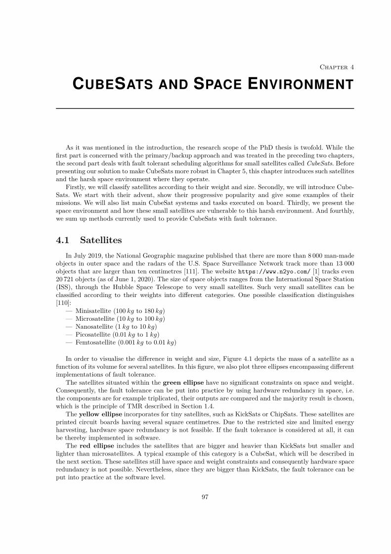
Chapter 4

CUBESATS AND SPACE ENVIRONMENT

As it was mentioned in the introduction, the research scope of the PhD thesis is twofold. While thefirst part is concerned with the primary/backup approach and was treated in the preceding two chapters,the second part deals with fault tolerant scheduling algorithms for small satellites called CubeSats. Beforepresenting our solution to make CubeSats more robust in Chapter 5, this chapter introduces such satellitesand the harsh space environment where they operate.

Firstly, we will classify satellites according to their weight and size. Secondly, we will introduce Cube-Sats. We start with their advent, show their progressive popularity and give some examples of theirmissions. We will also list main CubeSat systems and tasks executed on board. Thirdly, we present thespace environment and how these small satellites are vulnerable to this harsh environment. And fourthly,we sum up methods currently used to provide CubeSats with fault tolerance.

4.1 Satellites

In July 2019, the National Geographic magazine published that there are more than 8 000 man-madeobjects in outer space and the radars of the U.S. Space Surveillance Network track more than 13 000objects that are larger than ten centimetres [111]. The website https://www.n2yo.com/ [1] tracks even20 721 objects (as of June 1, 2020). The size of space objects ranges from the International Space Station(ISS), through the Hubble Space Telescope to very small satellites. Such very small satellites can beclassified according to their weights into different categories. One possible classification distinguishes[110]:

— Minisatellite (100 kg to 180 kg)— Microsatellite (10 kg to 100 kg)— Nanosatellite (1 kg to 10 kg)— Picosatellite (0.01 kg to 1 kg)— Femtosatellite (0.001 kg to 0.01 kg)

In order to visualise the difference in weight and size, Figure 4.1 depicts the mass of a satellite as afunction of its volume for several satellites. In this figure, we also plot three ellipses encompassing differentimplementations of fault tolerance.

The satellites situated within the green ellipse have no significant constraints on space and weight.Consequently, the fault tolerance can be put into practice by using hardware redundancy in space, i.e.the components are for example triplicated, their outputs are compared and the majority result is chosen,which is the principle of TMR described in Section 1.4.

The yellow ellipse incorporates for tiny satellites, such as KickSats or ChipSats. These satellites areprinted circuit boards having several square centimetres. Due to the restricted size and limited energyharvesting, hardware space redundancy is not feasible. If the fault tolerance is considered at all, it canbe thereby implemented in software.

The red ellipse includes the satellites that are bigger and heavier than KickSats but smaller andlighter than microsatellites. A typical example of this category is a CubeSat, which will be described inthe next section. These satellites still have space and weight constraints and consequently hardware spaceredundancy is not possible. Nevertheless, since they are bigger than KickSats, the fault tolerance can beput into practice at the software level.

97

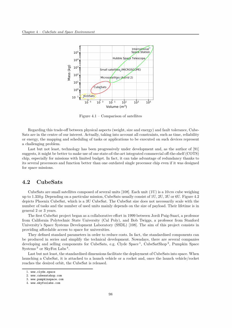
Chapter 4 – CubeSats and Space Environment

10−5 10−3 10−1 101 103 105Volume (m3)

10−1

100

101

102

103

104

105

Mass (kg)

Internati nal Space Stati n

Hubble Space Telesc pe

Small satellites (MICROSCOPE)

Micr satellites (Astrid 2)

CubeSats

KickSats

Figure 4.1 – Comparison of satellites

Regarding this trade-off between physical aspects (weight, size and energy) and fault tolerance, Cube-Sats are in the centre of our interest. Actually, taking into account all constraints, such as time, reliabilityor energy, the mapping and scheduling of tasks or applications to be executed on such devices representa challenging problem.

Last but not least, technology has been progressively under development and, as the author of [91]suggests, it might be better to make use of one state-of-the-art integrated commercial off-the-shelf (COTS)chip, especially for missions with limited budget. In fact, it can take advantage of redundancy thanks toits several processors and function better than one outdated single processor chip even if it was designedfor space missions.

4.2 CubeSats

CubeSats are small satellites composed of several units [108]. Each unit (1U) is a 10cm cube weighingup to 1.33kg. Depending on a particular mission, CubeSats usually consist of 1U, 2U, 3U or 6U. Figure 4.2depicts Phoenix CubeSat, which is a 3U CubeSat. The CubeSat size does not necessarily scale with thenumber of tasks and the number of used units mainly depends on the size of payload. Their lifetime is ingeneral 2 or 3 years.

The first CubeSat project began as a collaborative effort in 1999 between Jordi Puig-Suari, a professorfrom California Polytechnic State University (Cal Poly), and Bob Twiggs, a professor from StanfordUniversity’s Space Systems Development Laboratory (SSDL) [108]. The aim of this project consists inproviding affordable access to space for universities.

They defined standard parameters in order to reduce costs. In fact, the standardised components canbe produced in series and simplify the technical development. Nowadays, there are several companiesdeveloping and selling components for CubeSats, e.g. Clyde Space 1, CubeSatShop 2, Pumpkin SpaceSystems 3 or SkyFox Labs 4.

Last but not least, the standardised dimensions facilitate the deployment of CubeSats into space. Whenlaunching a CubeSat, it is attached to a launch vehicle or a rocket and, once the launch vehicle/rocketreaches the desired orbit, the CubeSat is released.

1. www.clyde.space

2. www.cubesatshop.com

3. www.pumpkinspace.com

4. www.skyfoxlabs.com

98

4.2. CubeSats

(a) Front view (b) Rear view

Figure 4.2 – Phoenix (3U) CubeSat (credit: Sarah Rogers, http://phxcubesat.asu.edu/)

At present, CubeSats become more and more popular. The number of launched CubeSats rapidlyincreases and is supposed to increase event more rapidly, as Figures 4.3 and 4.4 show. Graphs are takenfrom the nanosatellite database 5 [52] and they include also other satellites than CubeSats. Nevertheless,Figure 4.4 depicts that CubeSats account for the majority of considered satellites in the database.

The CubeSat project is a success and CubeSats are currently built not only at universities but alsoby space agencies, companies and other educational institutions, like high schools. Figure 4.5 shows thattwo main users are companies and universities.

The number of nanosatellites launched by countries is represented in Figure 4.6 and it can be seenthat nanosatellites are built throughout the world.

4.2.1 Mission

Regarding the CubeSat mission, they are primarily used for scientific investigations, most frequentlySpace Weather and Earth Science [108]. Several CubeSats also serve to test new design and equipment.Some examples of realised or scheduled CubeSat missions are as follows:

— Study the effects of the microgravity environment on biological cultures (GeneSat-1, 2003) 6

— Detect earthquakes (QuakeSat, 2003)[27]— Establish a radio connection, download telemetry and receive data from the telescope taking images

of the airglow emissions (SwissCube, 2009) [114]— Test a micro-propulsion system (amorphous hydrogenated Silicon solar cells), a new radio platform,

5. According to [52], the database includes and the term nanosatellite implies:— All CubeSats (0.25U to 27U),— Nanosatellites (1 kg to 10 kg),— Picosatellites (100 g to 1 kg),— PocketQubes, TubeSats, SunCunes and ThinSats

and the database does not include:— Femtosatellites (10 g to 100 g), chipsats and suborbital launches,— Satellite in idea or concept phase,— Data before 1998 (there were at least 21 nanosatellites launches in the 1960s and one in 1997).

6. https://directory.eoportal.org/web/eoportal/satellite-missions/g/genesat

99

Chapter 4 – CubeSats and Space Environment

Nanosatellite launches

2 10 2 7 422

9 10 14 19 1225

88

142129

88

297

244

188

458

222

85

31

343

435

468

545

www.nanosats.eu2020/04/20

1998

2000

2002

2003

2005

2006

2007

2008

2009

2010

2011

2012

2013

2014

2015

2016

2017

2018

2019

2020

2021

2022

20230

50

100

150

200

250

300

350

400

450

500

550

600

650

700

Nanosate

llit

es

Launched

Launch failures

Announced launch year

Nanosats.eu (2020 January) prediction

Figure 4.3 – Number of launched nanosatellites per year (As of April 20, 2020; taken from [52])

1998

1999

2000

2001

2002

2003

2004

2005

2006

2007

2008

2009

2010

2011

2012

2013

2014

2015

2016

2017

2018

2019

2020

0

100

200

300

400

500

600

700

800

900

1000

1100

1200

1300

0

500

1000

1500

2000

2500

3000

Total Nanosatellites & CubeSats Launched

2 2 12 12 14 21 21 2547 56 66 80

99 111136

224

366

495

583

880

1124

1312 1317

76

154

251

345

428

704

943

11091114

1210

67

www.nanosats.eu2020/04/20

Runnin

g t

ota

l of

sate

llit

es

Runnin

g t

ota

l of

CubeSat

unit

s

Nanosats launched incl. launch failures

CubeSats launched incl. launch failures

CubeSats deployed after reaching orbit

Nanosats with propulsion modules

CubeSats launched in total units

Figure 4.4 – Cumulative sum of launched nanosatellites (As of April 20, 2020; taken from [52])

an agile electrical power system and an active attitude control subsystem 7 (Delfi-n3XT, 2013)— Test the electric solar wind sail (ESTCUBE-1, 2013) [90]— Test the piezo motor activity in space, the position identification equipment and data processing

algorithms 8 (LituanicaSAT-1, 2014)

7. https://www.tudelft.nl/en/ae/delfi-space/delfi-n3xt/

8. http://www.litsat1.eu/en/

100

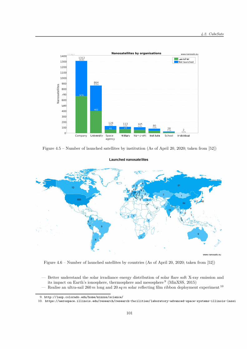
4.2. CubeSats

Nanosatellites by organisations

49.8%1312

32.8%864

4.9%128

4.3%113

4.0%1

3.0%80

1.1%28

0.1%2

6

402

61 7

www.nanosats.eu2

Company U Space

agency

M N !"o#t I$%&'()*+ School ,-./0345890

100

200

300

400

:;<

600

=>?

800

900

1000

1100

1200

1300

1400N

anosate

llit

es

L@ABCDEF

Not launched

Figure 4.5 – Number of launched satellites by institution (As of April 20, 2020; taken from [52])

Figure 4.6 – Number of launched satellites by countries (As of April 20, 2020; taken from [52])

— Better understand the solar irradiance energy distribution of solar flare soft X-ray emission andits impact on Earth’s ionosphere, thermosphere and mesosphere 9 (MinXSS, 2015)

— Realise an ultra-sail 260 m long and 20 sq m solar reflecting film ribbon deployment experiment 10

9. http://lasp.colorado.edu/home/minxss/science/

10. https://aerospace.illinois.edu/research/research-facilities/laboratory-advanced-space-systems-illinois-lassi

101

Chapter 4 – CubeSats and Space Environment

(CubeSail, 2018)— Test the concept of the new design of the deorbiting sail and test the new design of the sun sensor

device (PW-SAT2, 2018) [95]— Study Urban Heat Islands 11 (UHI) from Low Earth Orbit (LEO) through infrared sensing (PHX

SAT, 2019) [13]— Study atmospheric gravity waves 10 (LAICE, 2019)— Realise freeze-casting experiments to measure solidification velocity, dendrite and wall width, and

particle concentration 10 (SpaceICE, 2020)— Measure electron density (APSS, 2020) [93, 124]— Carry out the Earth’s imagery 12 (Doves, launched regularly) [84]Furthermore, researchers intend to use CubeSats also for the following missions:— Measure water quality using CubeSat hyperspectral imager [11]— Use constellations of CubeSats to monitor regions after a disaster, such as floods, landslides,

earthquakes or fires [127]— Use CubeSats to provide an alternative global coverage for the Internet of Things (IoT) and

Machine-to-machine (M2M) communications [8]Last but not least, designing and building of CubeSats at universities have also educational purposes.

In fact, students working together and putting into practice their knowledge gain rewarding experience.

4.2.2 Systems

CubeSats consist of several systems ensuring correct operations. Since the design can be fully developedby team or can be based on already prefabricated components, each CubeSat is unique. In general, if it isnecessary, each system has its own microcontroller (for example Texas Instruments MSP 430F1611 MCUused on board of SwissCube [114]) in order to provide basic housekeeping and parameter configuration,command execution and ensure communication with other systems. The commonly used systems are asfollows:

— On-Board Computer (OBC) or Command and Data Handling System (CDHS)This system executes the flight software. Their main functions are (i) to perform scheduling,execution and verification of telecommands, (ii) to store data from housekeeping and telemetry,(iii) to provide a time reference aboard, and (iv) to make computations for other CubeSat systems,for example the attitude determination and control system [40, 114].Since this system is responsible for the correct CubeSat operation, the choice of its microcontrolleris important. Several examples of used microcontrollers are summarised in Table 4.2. It can beseen that most CubeSats are based on the real-time operating system FreeRTOS.

— Attitude Determination and Control System (ADCS)This system consists of sensors, such as magnetometers, gyroscopes, sun or temperature sensors,and of magnetorquers used as actuators. The aim is to control the CubeSat attitude, i.e. to deter-mine the position, velocity and orientation [114]. Although the ADCS has its own microcontroller,it is used mainly to read sensors and control actuators. Data processing of the acquired data isgenerally processed by command and data handling system [40].This system is not used on board of each CubeSat because not all CubeSats require to direct inone particular direction. Therefore, it is used on board of satellites having for example a cameraas a payload.

— Electrical Power System (EPS)This system is responsible for electrical power generation, storage and management [100]. Thepower is harvested from sun using solar panels and stored in batteries. To illustrate the proportionof times in daylight and in eclipse (for a CubeSat located at the altitude of 600 km), a satellite

11. Urban Heat Islands is a phenomenon where cities tend to have warmer air temperatures than the surrounding rurallandscapes.

12. https://www.planet.com/

102

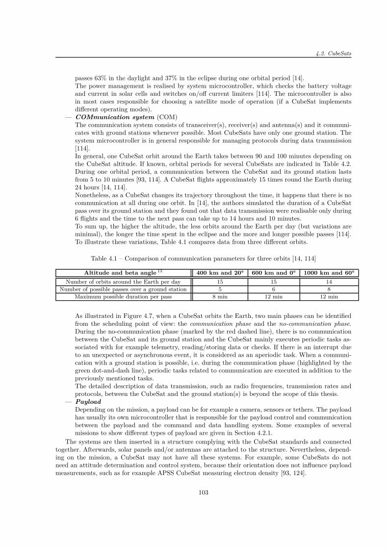
4.2. CubeSats

passes 63% in the daylight and 37% in the eclipse during one orbital period [14].The power management is realised by system microcontroller, which checks the battery voltageand current in solar cells and switches on/off current limiters [114]. The microcontroller is alsoin most cases responsible for choosing a satellite mode of operation (if a CubeSat implementsdifferent operating modes).

— COMmunication system (COM)The communication system consists of transceiver(s), receiver(s) and antenna(s) and it communi-cates with ground stations whenever possible. Most CubeSats have only one ground station. Thesystem microcontroller is in general responsible for managing protocols during data transmission[114].In general, one CubeSat orbit around the Earth takes between 90 and 100 minutes depending onthe CubeSat altitude. If known, orbital periods for several CubeSats are indicated in Table 4.2.During one orbital period, a communication between the CubeSat and its ground station lastsfrom 5 to 10 minutes [93, 114]. A CubeSat flights approximately 15 times round the Earth during24 hours [14, 114].Nonetheless, as a CubeSat changes its trajectory throughout the time, it happens that there is nocommunication at all during one orbit. In [14], the authors simulated the duration of a CubeSatpass over its ground station and they found out that data transmission were realisable only during6 flights and the time to the next pass can take up to 14 hours and 10 minutes.To sum up, the higher the altitude, the less orbits around the Earth per day (but variations areminimal), the longer the time spent in the eclipse and the more and longer possible passes [114].To illustrate these variations, Table 4.1 compares data from three different orbits.

Table 4.1 – Comparison of communication parameters for three orbits [14, 114]

Altitude and beta angle 13 400 km and 20° 600 km and 0° 1000 km and 60°

Number of orbits around the Earth per day 15 15 14

Number of possible passes over a ground station 5 6 8

Maximum possible duration per pass 8 min 12 min 12 min

As illustrated in Figure 4.7, when a CubeSat orbits the Earth, two main phases can be identifiedfrom the scheduling point of view: the communication phase and the no-communication phase.During the no-communication phase (marked by the red dashed line), there is no communicationbetween the CubeSat and its ground station and the CubeSat mainly executes periodic tasks as-sociated with for example telemetry, reading/storing data or checks. If there is an interrupt dueto an unexpected or asynchronous event, it is considered as an aperiodic task. When a communi-cation with a ground station is possible, i.e. during the communication phase (highlighted by thegreen dot-and-dash line), periodic tasks related to communication are executed in addition to thepreviously mentioned tasks.The detailed description of data transmission, such as radio frequencies, transmission rates andprotocols, between the CubeSat and the ground station(s) is beyond the scope of this thesis.

— PayloadDepending on the mission, a payload can be for example a camera, sensors or tethers. The payloadhas usually its own microcontroller that is responsible for the payload control and communicationbetween the payload and the command and data handling system. Some examples of severalmissions to show different types of payload are given in Section 4.2.1.

The systems are then inserted in a structure complying with the CubeSat standards and connectedtogether. Afterwards, solar panels and/or antennas are attached to the structure. Nevertheless, depend-ing on the mission, a CubeSat may not have all these systems. For example, some CubeSats do notneed an attitude determination and control system, because their orientation does not influence payloadmeasurements, such as for example APSS CubeSat measuring electron density [93, 124].

103

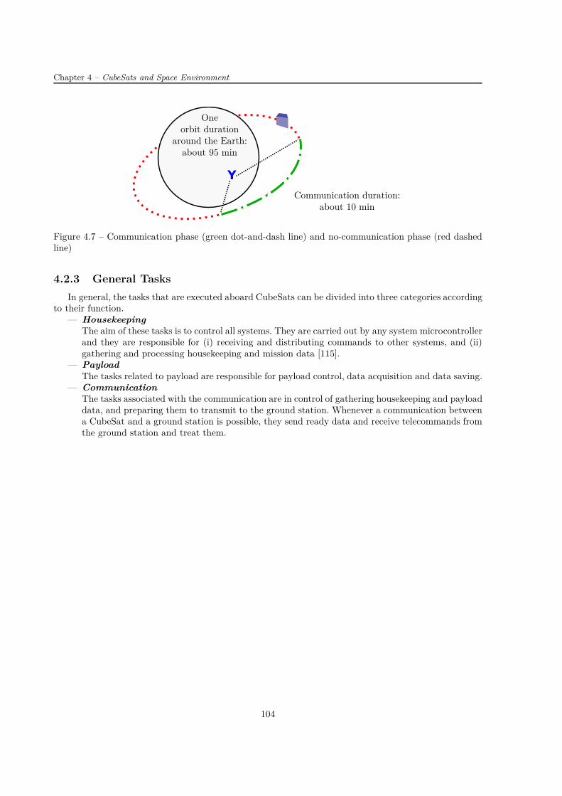
Chapter 4 – CubeSats and Space Environment

Y

Communication duration:about 10 min

Oneorbit duration

around the Earth:about 95 min

Figure 4.7 – Communication phase (green dot-and-dash line) and no-communication phase (red dashedline)

4.2.3 General Tasks

In general, the tasks that are executed aboard CubeSats can be divided into three categories accordingto their function.

— HousekeepingThe aim of these tasks is to control all systems. They are carried out by any system microcontrollerand they are responsible for (i) receiving and distributing commands to other systems, and (ii)gathering and processing housekeeping and mission data [115].

— PayloadThe tasks related to payload are responsible for payload control, data acquisition and data saving.

— CommunicationThe tasks associated with the communication are in control of gathering housekeeping and payloaddata, and preparing them to transmit to the ground station. Whenever a communication betweena CubeSat and a ground station is possible, they send ready data and receive telecommands fromthe ground station and treat them.

104

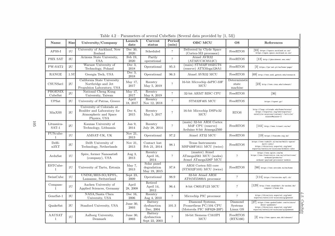
4.2

.C

ubeS

ats

Table 4.2 – Parameters of several CubeSats (Several data provided by [1, 53])

Name Size University/CompanyLaunch

dateCurrentstatus

Period(min)

OBC MCU OS References

APSS-I 1UUniversity of Auckland, New

ZealandDec 30,

2020Scheduled ?

Delivered by Clyde Space(Cortex-M3 processor)

FreeRTOS [93] https://space.auckland.ac.nz/

https://apss.space.auckland.ac.nz/

PHX SAT 3UArizona State University,

USAFeb 19,

2020Partly

operational?

Atmel AVR32(AT32UC3C0512C)

FreeRTOS [13] http://phxcubesat.asu.edu/

PW-SAT2 2UWarsaw University ofTechnology, Poland

Dec 3,2018

Operational 95.3(main) STM32F103ZGT6(reserve) ATXMega128A1

FreeRTOS [3] https://pw-sat.pl/en/home-page/

RANGE 1.5U Georgia Tech, USADec 3,2018

Operational 96.3 Atmel AVR32 MCU FreeRTOS [69] http://www.ssdl.gatech.edu/research

CSUNSat1 2UCalifornia State University

Northridge and JetPropulsion Laboratory, USA

May 17,2017

ReentryMay 5, 2019

?16-bit Microchip dsPIC-33F

MCU

Deterministicstate

machine[23] http://www.csun.edu/cubesat/

PHOENIXCubeSat

2UNational Cheng Kung

University, TaiwanMay 17,

2017Reentry

May 8, 2019? 32-bit ARM7 RISC CPU FreeRTOS [36]

UPSat 2U University of Patras, GreeceApril

18, 2017Reentry

Nov 12, 2018? STM32F405 MCU FreeRTOS https://upsat.gr/

MinXSS 3U

University of Colorado atBoulder and Laboratory for

Atmospheric and SpacePhysics, USA

Dec 6,2015

ReentryMay 5, 2017

?16-bit Microchip DSPic32

MCURTOS

http://lasp.colorado.edu/home/minxss/

https://eoportal.org/web/eoportal/

satellite-missions/content/-/article/

minxss#minxss-2

Lituanica-SAT-1

2UKaunas University ofTechnology, Lithuania

Jan 9,2014

ReentryJuly 28, 2014

?(main) 32-bit ARM Cortex

M4F CPU (reserve)Arduino 8-bit Atmega2560

FreeRTOS [141] http://www.litsat1.eu/en/

FUNcube-1

1U AMSAT-UK, UKNov 21,

2013Operational 97.2 Atmel AT32 MCU FreeRTOS [19] https://funcube.org.uk/

Delfi-n3XT

3UDelft University of

Technology, NetherlandsNov 21,

2013Contact lostFeb 21, 2014

98.1Texas Instruments

MSP430F1611 MCU (twice)FreeRTOS

https://www.tudelft.nl/en/ae/delfi-space/

delfi-n3xt/

https://directory.eoportal.org/web/

eoportal/satellite-missions/d/delfi-n3xt

ArduSat 1USpire, former Nanosatisfi

(company), USAAug 3,2013

ReentryApril 16,

2014?

(master) AtmelATmega2561 MCU (nodes)Atmel ATmega328P MCU

?https://www.spire.com/en

https://www.freetronics.com.au/collections/

ardusat/products/

ardusat-payload-processor-module

ESTCube-1

1U University of Tartu, EstoniaMay 7,2013

Solar paneldegradationMay 19, 2015

97.8ARM Cortex-M3 core

(STM32F103) MCU (twice)FreeRTOS [90] https://www.estcube.eu/en/home

SwissCube 1UUNINE/HES-SO/EPFL,Lausanne, Switzerland

Sept 23,2009

Operational 98.932-bit Atmel ARM

AT91M55800A processor? [114] https://swisscube.epfl.ch/

Compass-1

1UAachen University of

Applied Sciences, GermanyApril

28, 2008

RetiredApril 14,

201296.4 8-bit C8051F123 MCU ? [129] http://www.raumfahrt.fh-aachen.de/

compass-1/home.htm

GeneSat-1 3UNASA/Santa Clara

University, USADec 16,

2006Reentry

Aug 4, 2010? Microchip PIC processor ? https://directory.eoportal.org/web/

eoportal/satellite-missions/g/genesat

QuakeSat 3U Stanford University, USAJune 30,

2003

BatterydysfunctionDec, 2004

101.3Diamond Systems,

Prometheus PC/104 CPU(Motorola PIC 16F628-20P)

DiamondSystems

Linux OS

[27] https://www.quakefinder.com/science/

about-quakesat/

https://directory.eoportal.org/web/

eoportal/satellite-missions/q/quakesat

AAUSAT1

1UAalborg University,

DenmarkJune 30,

2003

Batterydysfunction

Sept 22, 2003?

16-bit Siemens C161IPIMCU

FreeRTOS(RTX166)

[2] http://www.space.aau.dk/cubesat/

105

Chapter 4 – CubeSats and Space Environment

4.3 Space Environment

Space is a harsh environment containing plasma, particle radiation, neutral gas particles, ultravioletand X-ray radiations, micrometeoroid and orbital debris [89]. From the viewpoint of satellites, theyoperate in void, under extreme temperature variations and intense accelerations and are subject to spaceradiation [115]. In this section, we will focus on the radiation because it causes faults in electronic devices.The higher the altitude, the more radiation effects. Although CubeSats are mostly situated at the lowEarth orbit (LEO), which is the lowest Earth orbit and located up to 2 000 km of altitude, the radiationshould be taken into account.

The space radiation has several sources and varies over time, as well as its effect on electronics [14].Its sources, depicted in Figure 4.8, are solar wind, solar energetic particles (such as solar flares), galacticcosmic rays, which are high energy particles, and particles trapped in the Earth’s magnetic field [22].Actually, when the radiation approaches the Earth, particles (mainly protons and electrons) are affectedby the Earth’s magnetic field and form radiation belts called Van Allen belts. They are two of them:inner and outer belts and they are located above the LEO. Nevertheless, as the true North does notexactly correspond with the magnetic North, the Earth’s magnetic field is asymmetric. This differencecauses high concentrations of particles at lower altitudes in the Atlantic near Argentina and Brazil. Thisphenomenon is called South Atlantic Anomaly (SAA). It is located at an altitude between 200 and 800km over the Earth’s surface and it presents a threat to spacecraft passing through [10, 14, 107, 109].

SGHJK Otlantic

PQRTVWX

YZ[\]^_`abc deld lines

Solar energetic particles

e

Solar wind

f

ghijklmn cosmic rays

Figure 4.8 – Space environment (Adapted from [10, Figure 2], [22, Slides 4 and 6] and [57, Figure 2.1]and satellite map taken from https://www.google.fr/maps)

The radiation effects are generally divided into two categories: (i) long-term, and (ii) transient orsingle particle effects [89].

The long-term effects are mainly due to protons and electrons, which accumulate on electroniccomponents. To evaluate this phenomenon, the metric called Total Ionising Dose (TID), also known asabsorbed radiation dose, is used. It accounts for the accumulation of ionising dose over time. This metricis habitually expressed in rad, where 1 rad = 0.01 J/kg. The material, which is considered, is mentionedin parentheses, e.g rad(Si) for silicon. Nonetheless, the unit of this metric in the international system isgray GY , where 1GY = 100rads [14, 22, 115]. Since materials have different characteristics, the choice ofthe material is important. For example, it was found in [34] that a GaAs random-access memory (RAM)is more sensitive to lower energy protons than the Si devices.

According to the National Aeronautics and Space Administration NASA [107], satellites and space

106

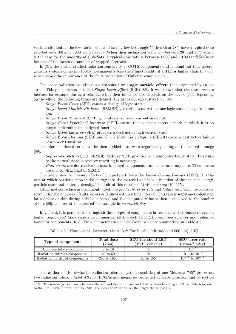
4.3. Space Environment

vehicles situated at the low Earth orbit and having low beta angle 13 (less than 28°) have a typical doserate between 100 and 1 000 rad(Si)/year. When their inclination is higher (between 20° and 85°), whichis the case for the majority of CubeSats, a typical dose rate is between 1 000 and 10 000 rad(Si)/yearbecause of the increased number of trapped electrons.

In [31], the author studied radiation sensitivity of COTS components and it found out that hetero-geneous systems on a chip (SoCs) permanently lose their functionality if a TID is higher than 15 krad,which shows the importance of the fault protection of CubeSat components.

The space radiation can also cause transient or single particle effects that originated by an ionstrike. This phenomenon is called Single Event Effect (SEE) [89]. It was shown that their occurrencesincrease for example during a solar flare but their influence also depends on the device [34]. Dependingon the effect, the following terms are defined (the list is not exhaustive) [78, 89]:

— Single Event Upset (SEU) causes a change of logic state.— Single Event Multiple Bit Error (SEMBE) gives rise to more than one logic state change from one

ion.— Single Event Transient (SET) generates a transient current in circuit.— Single Event Functional Interrupt (SEFI) causes that a device enters a mode in which it is no

longer performing the designed function.— Single Event Latch-up (SEL) provokes a destructive high current state.— Single Event Burnout (SEB) and Single Event Gate Rupture (SEGR) cause a destructive failure

of a power transistor.The aforementioned terms can be then divided into two categories depending on the caused damage

[89]:— Soft errors, such as SEU, SEMBE, SEFI or SET, give rise to a temporary faulty state. To return

to the normal state, a reset or rewriting is necessary.— Hard errors are destructive because impaired components cannot be used anymore. These errors

are due to SEL, SEB or SEGR.The metric used to measure effects of charged particles is the Linear Energy Transfer (LET). It is the

rate at which particles deposit the energy into the material and it is a function of the incident energy,particle mass and material density. The unit of this metric is MeV · cm2/mg [10, 115].

Other metrics, which are commonly used, are fault rate, error rate and failure rate. They respectivelyaccount for the number of faults, errors or failures within a time interval. This rate is sometimes calculatedfor a device or chip during a 24-hour period and the computed value is then normalized to the numberof bits [80]. The result is expressed for example in errors/bit-day.

In general, it is possible to distinguish three types of components in terms of their robustness againstfaults: commercial (also known as commercial off-the-shelf (COTS)), radiation tolerant and radiationhardened components [107]. Their characteristics at low Earth orbit are summarised in Table 4.3.

Table 4.3 – Component characteristics at low Earth orbit (altitude < 2 000 km) [107]

Type of componentsTotal dose

(krad)SEU threshold LET

(MeV · cm2/mg)SEU error rate(errors/bit-day)

Commercial components 2 to 10 5 10−5

Radiation tolerant components 20 to 50 20 10−7 to 10−8

Radiation hardened components 200 to 1000 80 to 150 10−10 to 10−12

The author of [10] devised a radiation tolerant system consisting of one Motorola 7457 processor,two radiation tolerant Actel AX2000 FPGAs and memories protected by error detection and correction

13. The beta angle is an angle between the sun and the orbit plane and it determines how long a LEO satellite is exposedto the Sun. It varies from −90° to +90°. The closer to 0° the value, the longer the eclipse [14].

107

Chapter 4 – CubeSats and Space Environment

(EDAC). The tests conducted on an orbit of 12 000 km altitude and the inclination of 10 degrees demon-strated that the overall system upset rate was 2.9 · 10−4 upsets/device/day and the failure rate of thesystem was approximately 1.5 · 10−6 per hour (not including radiation induced upsets).

More examples of data related to the fault occurrences have been already presented in Section 1.3. Forexample, Table 1.5 sums up the failure rates at the International Space Station and Table 1.3 summarisesthe fault/failures occurrences in space applications.

4.4 Fault Tolerance of CubeSats

Figure 4.9 depicts the present status of launched nanosatellites. Although it can be seen that themajority of launched nanosatellites (687 out of 1317 nanosatellites, i.e. 52.1%) are operational, the numberof launched nanosatellites, which are not operational, is high. In general, it is not easy to identify the reasonwhy a nanosatellite did not correctly function and failed, even if we can know for some nanosatellites thatthe failure occurred during the launch or during the deployment phase. In fact, these phases are mostvulnerable to failure.

opqrstuvw

xy

Not operationalz |~

t

Reentered

Returned

e

¡¢£

¤¥e0

¦§

100

¨©ª

200

«¬­

300

®¯°

400

±²³

´µ¶

·¸¹

600

º»¼

½¾¿

Present status of launched nanosatellites

ÀÁÂ

193

6 2

ÃÄÅ

8

ÆÇ

È

www.nanosats.euÉÊËÌÍÎÏÐÑÒ

ÓÔÕÖ×ØÙÚÛÜÝÞßà áâãäå æçèéd from: 7% (86 out of 1317)

Nanosate

llit

es

Figure 4.9 – Number of launched nanosatellites and their status (As of April 20, 2020; taken from [52])

In [92], the authors analysed the available satellite data and they found out that 20% of CubeSats aredead on arrival (DOA). Actually, nanosatellites experienced higher infant mortality and DOA rates whencompared to other larger satellites. This is mainly due to less testing prior to launch and consequentlysatellites are launched with undetected errors, which may cause a failure. Based on the analysis of failuredata, systematic errors, e.g. failures in design and manufacturing, are the most frequent sources of satellitefailure [91]. Moreover, when a CubeSat is transported by a rocket or a launch vehicle to the desired orbit,it must be completely electrically neutral, which means that its batteries must be flat. Once a CubeSatis released in the space, it needs to harvest energy and boot itself [124].

Furthermore, the author of [91] analysed statistical data (mainly based on analysis of 1 584 satellitesstudied in "Spacecraft Reliability and Multi-State Failures" (2011) by J. H. Saleh and J.-F. Castet) andconcluded that, if a satellite is correctly deployed, its projected lifetime (2 or 3 years) will be achievedwith probability of more than 90%. Moreover, he stated that, if a failure occurs, 82% of failures is dueto software and remaining percents are caused by hardware. Although larger satellites have lower infant

108

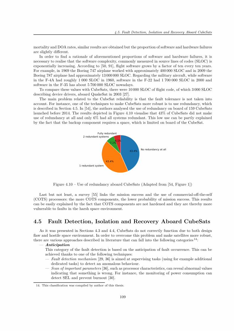
4.5. Fault Detection, Isolation and Recovery Aboard CubeSats

mortality and DOA rates, similar results are obtained but the proportion of software and hardware failuresare slightly different.

In order to find a rationale of aforementioned proportions of software and hardware failures, it isnecessary to realise that the software complexity, commonly measured in source lines of codes (SLOC) isexponentially increasing. According to [50, 91], flight software grows by a factor of ten every ten years.For example, in 1969 the Boeing 747 airplane worked with approximately 400 000 SLOC and in 2009 theBoeing 787 airplane had approximately 13 000 000 SLOC. Regarding the military aircraft, while softwarein the F-4A had roughly 1 000 SLOC in 1960, software in the F-22 had 1 700 000 SLOC in 2000 andsoftware in the F-35 has about 5 700 000 SLOC nowadays.

To compare these values with CubeSats, there were 10 000 SLOC of flight code, of which 3 000 SLOCdescribing device drivers, aboard QuakeSat in 2003 [27].

The main problem related to the CubeSat reliability is that the fault tolerance is not taken intoaccount. For instance, one of the techniques to make CubeSats more robust is to use redundancy, whichis described in Section 4.5. In [54], the authors analysed the use of redundancy on board of 159 CubeSatslaunched before 2014. The results depicted in Figure 4.10 visualise that 43% of CubeSats did not makeuse of redundancy at all and only 6% had all systems redundant. This low use can be partly explainedby the fact that the backup component requires a space, which is limited on board of the CubeSat.

No redundancy at all43.4%

1 redundant system43.4%

2 redundant systems

7.1%

Fully redundant

6.1%

Figure 4.10 – Use of redundancy aboard CubeSats (Adapted from [54, Figure 1])

Last but not least, a survey [55] links the mission success and the use of commercial-off-the-self(COTS) processors: the more COTS components, the lower probability of mission success. This resultscan be easily explained by the fact that COTS components are not hardened and they are thereby morevulnerable to faults in the harsh space environment.

4.5 Fault Detection, Isolation and Recovery Aboard CubeSats

As it was presented in Sections 4.3 and 4.4, CubeSats do not correctly function due to both designflaw and hostile space environment. In order to overcome this problem and make satellites more robust,there are various approaches described in literature that can fall into the following categories 14:

— AnticipationThis category of the fault detection is based on the anticipation of fault occurrence. This can beachieved thanks to one of the following techniques:— Fault detection mechanism [29, 36] is aimed at supervising tasks (using for example additional

dedicated tasks) to detect an anomalous behaviour.— Scan of important parameters [36], such as processor characteristics, can reveal abnormal values

indicating that something is wrong. For instance, the monitoring of power consumption candetect SEL and prevent burnout [30].

14. This classification was compiled by author of this thesis.

109

Chapter 4 – CubeSats and Space Environment

— Analysis of error reports [36, 90] allows users to find reasons for failure occurrences and conse-quently to upgrade the system to be able to tolerate such faults in the future. A rectificationcan be made directly in the code or a correction can be defined in a library describing how torecover from failures [36].

— Kalman filtering is sometimes used as an advanced technique to predict the satellite conditionin the future and detect a failure [29]. Due to its complexity, it is not commonly put intopractice on board of CubeSats. A rare example of its implementation is ESTCube-1 [90].

— Turning off processors improves the system reliability because switched off components are lessvulnerable to faults. This technique is not often used on board of CubeSats but it is employedaboard the Hubble Space Telescope. In fact, when it passes through the South Atlantic Anomaly(described in Section 4.3), it does not carry out any observation [57].

— Last but not least, prior tests before launch [29] make possible to detect faults and correctthem before the beginning of the mission.

— RedundancyIn order to fulfil a mission, it is recommended to have a backup component able to take overthe duties of the first component if it becomes faulty [3, 29, 36, 141]. In literature, two types aredistinguished: hot redundancy and cold redundancy [90]. The backup components using the formertype are always turned on so that they are ready to immediately provide results in the case thefirst component is faulty. When the latter type is put into practice, the backup components areturned off and switched on once the first component is unable to correctly function. Nevertheless,due to space constraints aboard CubeSats, it may not be possible to make use of this fault toleranttechnique.As an example, we consider the use of redundancy for on-board computer, which represents animportant part of CubeSat because its malfunction jeopardises the mission. In [3], the authorsdifferentiated three cases:— If only one microcontroller is used, there is no redundancy and, in case of dysfunction, the

mission is aborted. This solution is often chosen and was used for example on board of AAUSat,Compass-1 Picosatellite, PHOENIX CubeSat or SWEET CubeSat.

— In order to use a redundancy, two identical and independent microcontrollers can be put onboard. A drawback of this approach is that two identical microcontrollers are subject to spaceenvironment, in particular to ionizing radiation, at similar rate. Therefore, it is likely that thebackup component will malfunction soon after the first one. This solution was chosen by teamdesigning the ESTCube-1 [90].

— To overcome the problem related to the degradation at similar rate, two different independentmicrocontrollers can be applied. The main microcontroller ensures smooth operation of themission. If it becomes defective, a backup microcontroller takes over its function. It is lesspowerful but able to execute vital tasks so that the mission could continue despite degradedfunctioning. Since the second component is less advanced, it degrades slowly than the mainone. This approach was chosen for PW-Sat2 [3].

— Watchdog timer and reset/rebootIf a system malfunctions, for example it is latched up or frozen, one of the possibilities is to reboot orreset the system. A commonly used technique is the watchdog timer [3, 29, 30, 36, 38, 100, 114, 141].In principle, if time is up, for example if a watchdog does not receive a heartbeat from a processorwithin the defined time [27], software is reset and/or a satellite is rebooted.Although this solution is usually used to recover from a faulty state, it can be periodically employedto avoid a fault occurrence. For instance, QuakeSat rebooted the system every two weeks [27].

— CheckpointingThis method consists in periodic saving of data during the execution. If a fault occurs, while a taskis executing, its execution is restarted from the last checkpoint or from scratch if no checkpointexists. On board of satellites, this technique was put into practice for example in [56].

— Remote control

110

4.6. Summary

Since there is a regular communication between a CubeSat and ground stations, the CubeSattransmits reports on its current status. These reports can be analysed and operators can sendtelecommands in order to configure or upgrade on-board software during the mission [29, 38, 90].

— Safe modeIf a fault is detected, the command and data handling system can decide that the CubeSat switchesits state machine to the safe mode [29, 38, 114, 141]. To quit this state, a system needs to recoverfrom fault, e.g. thanks to the reboot or telecommands sent by operators.

— Data protectionFaults can also occur when transmitting data or when accessing memory, i.e. during reading orstoring data. Techniques for data protection are usually based on information redundancy, whichadds check bits to data in order to verify the correctness [85]. The commonly used techniques arethe checksum [38], cyclic redundancy checks (CRC) [36] and Hamming codes [30, 38].It is also possible to triplicate the memory [23, 90] or interconnect all systems together to avoid afailure in communication [90].

— Radiation hardened componentsA possibility of dealing with radiation is to use components designed for the harsh space environ-ment. Nevertheless, they are rather expensive and not all teams can afford them [10, 19]. Table 4.3compares radiation hardened and commercial off-the-shelf components in terms of the capabilityto withstand the radiation.

— ShieldingShielding is a simple method to protect a component or the whole system against radiation [10, 30].This method cannot reflect all particles but it reduces their number. Since each component (evena COTS one) has a certain level of the radiation sensitivity, the aim of shielding is not to exceedthis level. However, shielding is not applicable to all types of radiation. It is an efficient protectionagainst TID but useless against single event effects.In [31], the authors studied fault tolerance of satellite on-board computers based on COTS com-ponents. They found out that an aluminium shielding of 1.5 mm is sufficient for a small satelliteto correctly function during 3 years, which generally corresponds to the end of a typical missionlength.Since CubeSats have strict weight constraints, the main drawback of this method is the increasein the total satellite mass.

4.6 Summary

This chapter presented CubeSats and the harsh space environment where they operate. Althoughthey become more and more popular thanks to the standardisation of components and rather affordablebudget, their missions are not always fulfilled. One of the main causes is that CubeSats are not so robustas they should be to withstand faults caused for example by radiation. No matter the reason of the lackof fault tolerance (for example budget or space constraints), a solution to make CubeSats more robustagainst faults is one of the main achievements of this thesis and is presented in the next chapter.

111

Chapter 5

ONLINE FAULT TOLERANT SCHEDULING

ALGORITHMS FOR CUBESATS

The preceding chapter introduced small satellites called CubeSats, which become more and morepopular and are built not only at universities but also by companies and space agencies [52]. It wasshown that since they operate in the harsh space environment and the fault tolerance is not alwaysconsidered due to for example budget or time constraints, they are vulnerable to faults.

To support CubeSat teams, this chapter comes up with a solution to make CubeSats more faulttolerant. After the introduction of the idea, we present our system, task and fault models. Then thealgorithms and experimental framework are described. Subsequently we carry out the analysis and discussthe results.

We present two no-energy-aware algorithms, OneOff and OneOff&Cyclic, and then one energy-aware algorithm called OneOffEnergy.

5.1 Our Idea

Our aim is to provide CubeSats with the fault tolerance. As there are several systems aboard CubeSatsand most of them have its own processor, we present a solution gathering all processors on one board. Thismodification will not only reduce space and weight and optimise the energy consumption but also improvethe system resilience. First, a shielding against radiation will be easier to put into practice [30, 31], asdescribed in Section 4.5. Second, a CubeSat will remain operational even in case of a permanent processorfailure, because processors are not dedicated to one system (as it is done in current CubeSats) and eachprocessor can execute any task. Although this design is not typical nowadays, it has been successfullyrealised for example on board of ArduSat, which has 17 processors on one board [58].

Once all processors are gathered on one board, we intend to use the proposed scheduling algorithmsdealing with all tasks (regardless of the system) on board of any CubeSat or any small satellite. Thesealgorithms schedule all types of tasks (periodic, sporadic and aperiodic), detect faults and take appropriatemeasures to provide correct results. They are executed online in order to promptly manage occurring faultsand respect real-time constraints. They are mainly meant for CubeSats based on commercial-off-the-shelf(COTS) processors, which are not necessarily designed to be used in space applications and thereforemore vulnerable to faults than radiation hardened processors. It was reported [55] that the more COTScomponents in a CubeSat, the lower the probability of its mission success.

5.2 No-Energy-Aware Algorithms

5.2.1 System, Fault and Task Models

Table 5.1 summarises notations and definitions used in our research related to CubeSats.The studied system consists of P interconnected identical processors. Although the system is composed

of homogeneous processors sharing the same memory, it would be possible to extend it to a systemcomposed of heterogeneous processors, like in [155]. The system handles all tasks on board of the CubeSat.

113

Chapter 5 – Online Fault Tolerant Scheduling Algorithms for CubeSats

Table 5.1 – Notations and definitions

Notation Definition

ai Arrival time of task ti

φi Phase of task ti

Ti Period of task ti

eti Execution time of task ti

di Deadline of task ti

tti Task type of task ti

α Multiple of eti to define the size of PC scheduling window

P Ci Primary copy of task ti

BCi Backup copy of task ti

xCi P C or BC of task ti

start(xCi) Start of the execution of P Ci or BCi

end(xCi) End of the execution of P Ci or BCi

S Simple task

D Double task

These tasks are mostly related to housekeeping (e.g. sensor measurements), communication with groundstation and storing or reading data from the memory.

The task model distinguishes aperiodic and periodic tasks. An aperiodic task, depicted in Figure 5.1,is characterised by arrival time ai, execution time eti, deadline di and task type tti, which will be definedin the next paragraph. A periodic task, represented in Figure 5.2, has several instances and has fourattributes: φi (which is the arrival time of the first instance), execution time eti, period Ti and task typetti. We consider that the relative deadline equals the period. For both aperiodic and periodic tasks, atask must be executed respectively before the deadline or the beginning of the next period.

eti

task window

ai di

Figure 5.1 – Model of aperiodic task ti

eti

Ti

φi φi + Ti φi + (k − 1) · Ti

kth instance

Figure 5.2 – Model of periodic task τi [33]

The fault model considers both transient and permanent faults and it distinguishes two task types:simple (S) and double (D) tasks depending on the fault detection. For both task types, we distinguish twotypes of task copies: primary copy (PC) and backup copy (BC). The former copies are necessary for taskexecution in a fault-free environment. If and only if a primary copy is faulty, the corresponding backupcopy is scheduled. The algorithm consequently schedules backup copies only when it is necessary, whichavoids waste of resources.

Simple tasks have only one primary copy because a fault is detected by timeout, no received acknowl-edgment or failure of data checks. By contrast, a fault detection for double tasks requires the execution oftwo primary copies 1 and then their comparison because fault detection techniques for simple tasks maynot be sufficient to detect a fault. We consider that a scheduler is robust, e.g. data related to scheduling,such as task queues, are duplicated in memory or the system has a spare one if necessary.

Our objective is to minimise the task rejection rate subject to real-time and reliability constraints,which means maximising the number of tasks being correctly executed before deadline even if a faultoccurs.

1. Two task copies of the same task ti can overlap each other on different processors but it is not necessary. However,they must not be executed on one processor in order to be able to detect a faulty processor.

114

5.2. No-Energy-Aware Algorithms

Therefore, using Graham’s notation [66] described in Section 1.1, the studied problem is defined as:

P ; m | n = k; online rj ; dj = d; pj = p | (minimise the rejection rate)

which means that k independent jobs/tasks (characterised by release time rj , processing time pj anddeadline dj) arrive online on a system consisting of m parallel identical machines and are scheduled tominimise the rejection rate.

5.2.2 Presentation of Algorithms

This section describes two algorithms meant for online global scheduling on a multiprocessor system.First of all, it starts with several general principles applicable for both of them.

All tasks arriving to the system are ordered in a task queue using different policies. In order not toincrease the algorithm run-time, we analyse several underlying ordering policies at the beginning to finallychoose one policy minimising the rejection rate. The policies for aperiodic tasks are as follows: Random,Minimum Slack (MS) first, Highest ratio of eti to (di-t) first, Lowest ratio of eti to (di-t) first, LongestExecution Time (LET) first, Shortest Execution Time (SET) first, Earliest Arrival Time (EAT) first andEarliest Deadline (ED) first; and the ones for periodic tasks are as reads: Random, Minimum Slack (MS)first, Longest Execution Time (LET) first, Shortest Execution Time (SET) first, Earliest Phase (EP) firstand Rate Monotonic (RM).

A preemption is not authorised but the task rejection is allowed. A task ti is rejected at time t andremoved from the task queue if its task copies do not meet its deadline, i.e. t + eti > di for the aperiodictask or t + eti > φi + k · Ti for the kth instance of periodic task. We remind the reader that a simple taskti has one PC (denoted by P Ci), whereas a double task ti has two PCs (respectively labelled P Ci,1 andP Ci,2) in a fault-free environment.

execution time

start time(ai or φi + (k − 1) · Ti)

deadline - α · eti deadline(di or φi + k · Ti)

Figure 5.3 – Principle of scheduling task copies

As Figure 5.3 shows, all primary copies are scheduled as soon as possible to avoid idle processors justafter task arrival and possible high processor load later. As our goal is to minimise the task rejection, thealgorithm reserves a certain time of the task window to place a backup copy if the PC execution is faulty.The end of the PC scheduling window is defined as di −α ·eti for the aperiodic task and φi +k ·Ti −α ·eti

for the kth instance of periodic task (with α > 1). We consider without loss of generality that α = 1.When the algorithm finds out that a primary copy was faulty, the corresponding backup copy is

scheduled and can start its execution immediately, i.e. even during the PC scheduling window, becauseits results are necessary. The proposed algorithms guarantee that, if any primary copy is faulty, itscorresponding backup copy can be always scheduled and executed. Actually, from the scheduling point ofview, the backup copies of all accepted tasks can always be scheduled and executed. Nevertheless, it mayhappen that a backup copy is impacted by a fault too. Therefore, we distinguish two metrics, described inSection 5.2.3.2 to evaluate both the system schedulability by means of the rejection rate and the numberof correctly executed tasks by the system throughput.

Regarding the processor allocation, we call the slot, a time interval within the processor schedule. Thealgorithm starts to check the first free slot on each processor and then, if a solution was not found, itcontinues with next slots (second, third, ...) until a solution is obtained or all free slots on all processorsare tested. This processor allocation strategy corresponds to the one we proposed for the primary/backupapproach and called the first found solution search slot by slot. It is described in Section 3.1.1.2. Although

115

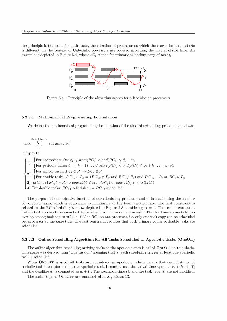
Chapter 5 – Online Fault Tolerant Scheduling Algorithms for CubeSats

the principle is the same for both cases, the selection of processor on which the search for a slot startsis different. In the context of CubeSats, processors are ordered according the first available time. Anexample is depicted in Figure 5.4, where xCi stands for primary or backup copy of task ti.

Figure 5.4 – Principle of the algorithm search for a free slot on processors

5.2.2.1 Mathematical Programming Formulation

We define the mathematical programming formulation of the studied scheduling problem as follows:

maxSet of tasks∑

i

ti is accepted

subject to

1)

For aperiodic tasks: ai 6 start(P Ci) < end(P Ci) 6 di − eti

For periodic tasks: φi + (k − 1) · Ti 6 start(P Ci) < end(P Ci) 6 φi + k · Ti − α · eti

2)

For simple tasks: P Ci ∈ Px ⇒ BCi /∈ Px

For double tasks: P Ci,1 ∈ Px ⇒ (P Ci,2 /∈ Px and BCi /∈ Px) and P Ci,2 ∈ Py ⇒ BCi /∈ Py

3) (xCi and xCj) ∈ Px ⇒ end(xCi) 6 start(xCj) or end(xCj) 6 start(xCi)4) For double tasks: P Ci,1 scheduled ⇔ P Ci,2 scheduled

The purpose of the objective function of our scheduling problem consists in maximising the numberof accepted tasks, which is equivalent to minimising of the task rejection rate. The first constraint isrelated to the PC scheduling window depicted in Figure 5.3 considering α = 1. The second constraintforbids task copies of the same task to be scheduled on the same processor. The third one accounts for nooverlap among task copies xC (i.e. P C or BC) on one processor, i.e. only one task copy can be scheduledper processor at the same time. The last constraint requires that both primary copies of double tasks arescheduled.

5.2.2.2 Online Scheduling Algorithm for All Tasks Scheduled as Aperiodic Tasks (OneOff)

The online algorithm scheduling arriving tasks as the aperiodic ones is called OneOff in this thesis.This name was derived from "One task off" meaning that at each scheduling trigger at least one aperiodictask is scheduled.

When OneOff is used, all tasks are considered as aperiodic, which means that each instance ofperiodic task is transformed into an aperiodic task. In such a case, the arrival time ai equals φi +(k−1)·Ti

and the deadline di is computed as ai + Ti. The execution time eti and the task type tti are not modified.The main steps of OneOff are summarised in Algorithm 13.

116

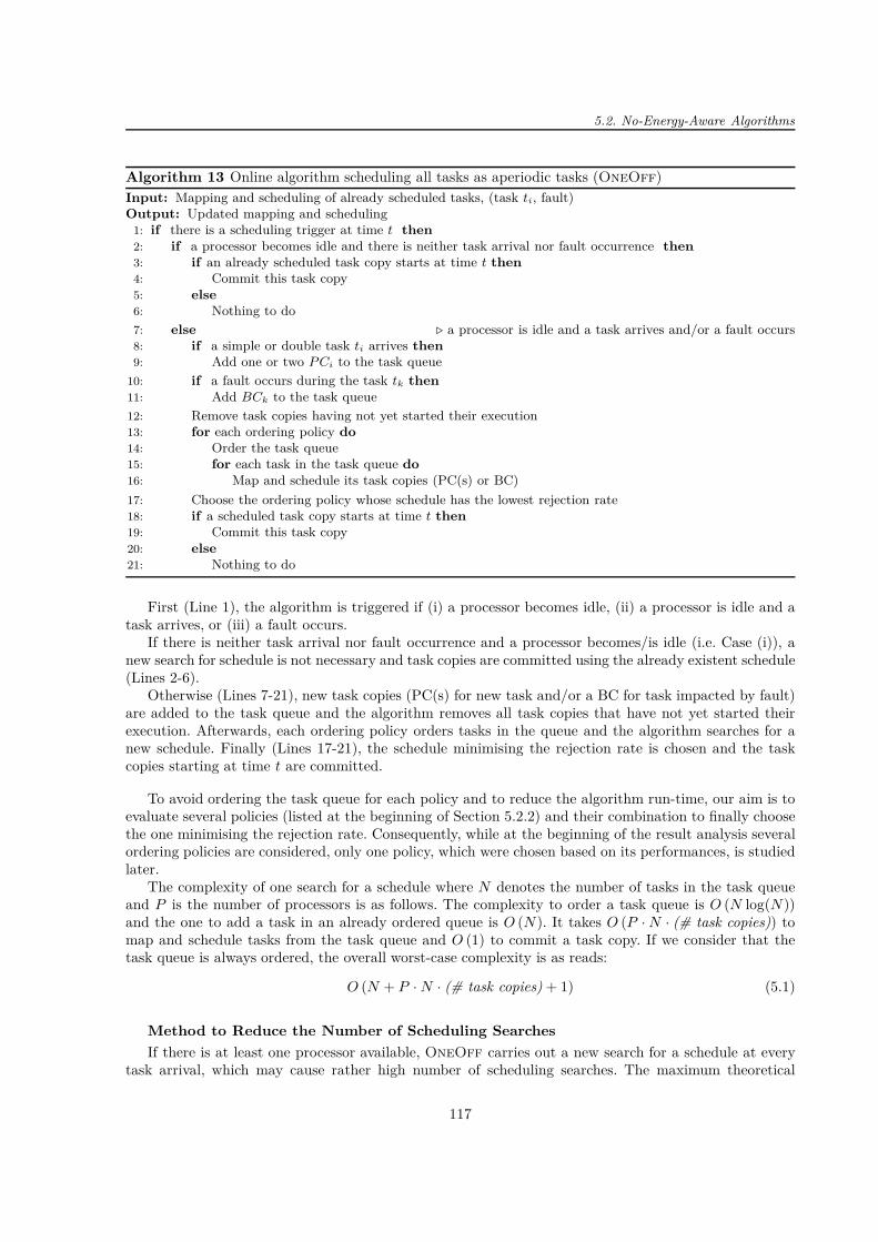
5.2. No-Energy-Aware Algorithms

Algorithm 13 Online algorithm scheduling all tasks as aperiodic tasks (OneOff)Input: Mapping and scheduling of already scheduled tasks, (task ti, fault)Output: Updated mapping and scheduling

1: if there is a scheduling trigger at time t then2: if a processor becomes idle and there is neither task arrival nor fault occurrence then3: if an already scheduled task copy starts at time t then4: Commit this task copy5: else6: Nothing to do

7: else ⊲ a processor is idle and a task arrives and/or a fault occurs8: if a simple or double task ti arrives then9: Add one or two P Ci to the task queue

10: if a fault occurs during the task tk then11: Add BCk to the task queue

12: Remove task copies having not yet started their execution13: for each ordering policy do14: Order the task queue15: for each task in the task queue do16: Map and schedule its task copies (PC(s) or BC)

17: Choose the ordering policy whose schedule has the lowest rejection rate18: if a scheduled task copy starts at time t then19: Commit this task copy20: else21: Nothing to do

First (Line 1), the algorithm is triggered if (i) a processor becomes idle, (ii) a processor is idle and atask arrives, or (iii) a fault occurs.

If there is neither task arrival nor fault occurrence and a processor becomes/is idle (i.e. Case (i)), anew search for schedule is not necessary and task copies are committed using the already existent schedule(Lines 2-6).

Otherwise (Lines 7-21), new task copies (PC(s) for new task and/or a BC for task impacted by fault)are added to the task queue and the algorithm removes all task copies that have not yet started theirexecution. Afterwards, each ordering policy orders tasks in the queue and the algorithm searches for anew schedule. Finally (Lines 17-21), the schedule minimising the rejection rate is chosen and the taskcopies starting at time t are committed.

To avoid ordering the task queue for each policy and to reduce the algorithm run-time, our aim is toevaluate several policies (listed at the beginning of Section 5.2.2) and their combination to finally choosethe one minimising the rejection rate. Consequently, while at the beginning of the result analysis severalordering policies are considered, only one policy, which were chosen based on its performances, is studiedlater.

The complexity of one search for a schedule where N denotes the number of tasks in the task queueand P is the number of processors is as follows. The complexity to order a task queue is O (N log(N))and the one to add a task in an already ordered queue is O (N). It takes O (P · N · (# task copies)) tomap and schedule tasks from the task queue and O (1) to commit a task copy. If we consider that thetask queue is always ordered, the overall worst-case complexity is as reads:

O (N + P · N · (# task copies) + 1) (5.1)

Method to Reduce the Number of Scheduling Searches

If there is at least one processor available, OneOff carries out a new search for a schedule at everytask arrival, which may cause rather high number of scheduling searches. The maximum theoretical

117

Chapter 5 – Online Fault Tolerant Scheduling Algorithms for CubeSats

number of scheduling searches is as follows:

(maximum theoretical # of scheduling searches) = (# tasks at the input) + (# task copies) (5.2)

In order to reduce this number, we present a method making use of a buffer, which is a commonlyused technique in scheduling [46, 81]. It computes the slack for every task ti and checks whether or not asearch for a new schedule can be postponed. The slack stands for the remaining time between the currenttime and the task deadline. The slack is called short if

di − current time − eti 6 K · eti where K ∈ N (5.3)

otherwise, it is called large.The principle of the method is illustrated in Figure 5.5. The highlighted background shows the part

that was added to the baseline version. To enter it, the algorithm checks the slack using Formula 5.3where K = β and the current time equals the task arrival. If the computed slack is large, the task is putinto the buffer. Otherwise, it is scheduled as usual.

The tasks stored in the buffer of length L are scheduled if the buffer is full. In order to regularly checkslacks of tasks queuing in the buffer, a verification (with K = γ) is carried out if a new task arrives inthe buffer or a processor becomes idle. If any task has a short slack, the buffer is emptied and all tasksscheduled.

Figure 5.5 – Principle of the method to reduce the number of scheduling searches

5.2.2.3 Online Scheduling Algorithm for All Tasks Scheduled as Aperiodic or PeriodicTasks (OneOff&Cyclic)

The online algorithm scheduling arriving tasks as the aperiodic or periodic ones is called One-Off&Cyclic. Its name is derived from OneOff. The term Cyclic is appended because the algorithm isalso able to deal with the periodic tasks and to repeat an already determined schedule of one hyperperiod(HT) until a new scheduling trigger occurs.

OneOff&Cyclic is consequently aware that there are not only aperiodic tasks but also periodicones and there are two task sets: one for periodic tasks and one for aperiodic ones.

The main steps of OneOff&Cyclic are summed up in Algorithm 14.

118

5.2. No-Energy-Aware Algorithms

Algorithm 14 Online algorithm scheduling all tasks as periodic or aperiodic tasks (OneOff&Cyclic)Input: Mapping and scheduling of already scheduled tasks, (task ti, fault)Output: Updated mapping and scheduling

1: if there is a scheduling trigger at time t then2: if a processor becomes idle and there is neither arrival/withdrawal of periodic task nor arrival of aperiodic

task nor fault occurrence then3: if an already scheduled task copy starts at time t then4: Commit this task copy5: else6: Nothing to do

7: else ⊲ a processor is idle and there is a change in set of periodic or aperiodic tasks and/or a fault occurs8: if a periodic task ti arrives or is withdrawn then9: Add/withdraw one or two P Ci to/from the queue of periodic tasks

10: if an aperiodic task ti arrives then11: Add one or two P Ci to the queue of aperiodic tasks

12: if a fault occurs during the task tk then13: Add BCk to the queue of aperiodic tasks

14: Remove task copies having not yet started their execution15: for each ordering policy do16: Order the task queues17: for each task in the task queue of aperiodic tasks do18: Map and schedule its task copies (PC(s) or BC)

19: for each task in the task queue of periodic tasks do20: Map and schedule its task copies (PC(s) or BC)

21: Choose the ordering policy whose schedule has the lowest rejection rate22: if a scheduled task copy starts at time t then23: Commit this task copy24: else25: Nothing to do

First (Line 1), the algorithm is triggered (i) if a processor becomes idle, and/or if there is (ii) anarrival of aperiodic task(s), (iii) an arrival/withdrawal 2 of periodic task(s), or (iv) a fault during taskexecution.

In the case a processor becomes idle (Case (i)), a new search for schedule is not carried out and taskcopies are committed using the already determined schedule (Lines 2-6). As there is no modification intask sets, the schedule of one hyperperiod, which is the least common multiple of task periods, is repeateduntil one of Cases (ii)-(iv) occurs.

Otherwise (Lines 7-25), the task sets of periodic and aperiodic tasks are updated and all task copiesthat have not yet started their execution, are removed from the former schedule. Afterwards (Lines 16-20), task sets are ordered and the algorithm schedules aperiodic tasks and periodic ones. In general, sincethere are none or only a few tasks in a set of aperiodic tasks (accounting mainly for interrupts), thechoice of ordering policy is not important compared to the one for periodic tasks. Finally (Lines 21-25),the schedule minimising the rejection rate is chosen and the task copies starting at time t are committed.

Again, our goal is to assess several ordering policies (listed at the beginning of Section 5.2.2) and theircombination to select the one minimising the rejection rate in order to avoid ordering the task queueseveral times and reduce the algorithm run-time. Consequently, while at the beginning of the resultanalysis several ordering policies for periodic tasks are considered, only one policy is studied later.

Similarly to OneOff, we denote Naper as the number of aperiodic task in the task queue and Nper asthe number of task instances per hyperperiod of periodic tasks in the task queue. The overall worst-case

2. A possibility to add or withdraw a periodic task from the task set allows us to model sporadic tasks related to thecommunication between a CubeSat and a ground station. More details are presented in Section 5.2.3.

119

Chapter 5 – Online Fault Tolerant Scheduling Algorithms for CubeSats

complexity is as reads:

O(Naper + P · Naper · (# task copies) + Nper + P · Nper · (# task copies) + 1) (5.4)

5.2.3 Experimental Framework

In Section 4.2.2, it was mentioned that two main phases during the CubeSat orbit can be identifiedfrom the scheduling point of view: the communication and no-communication phases, as depicted inFigure 4.7. Recall that CubeSats mainly execute periodic tasks related to e.g. telemetry, reading/storingdata or checks. Interrupts due to an unexpected or asynchronous event are considered as aperiodic tasks.These tasks are executed during both communication and no-communication phases. In addition, duringthe communication phase, CubeSats deal with tasks associated with the communication. Since thesetasks are periodically repeated when a communication takes place, but are not present during the no-communication phase, they are called sporadic.

Next, we describe our simulation scenario and define metrics employed to analyse the presentedalgorithms.

5.2.3.1 Simulation Scenario

The data exploited in our experimental framework are based on real CubeSat data provided by theAuckland Program for Space Systems (APSS) 3 and by the Space Systems Design Lab (SSDL) 4. Thesedata were gathered by their functionality and generalised in order to generate more data for simulations.They are respectively called Scenario APSS and Scenario RANGE and summarised in Tables 5.2 and 5.3,where U denotes a uniform distribution, the arbitrary time unit is 1 ms and one hyperperiod is the leastcommon multiple of task periods.

Table 5.2 – Set of tasks for Scenario APSS

Periodic tasks

Function Task type tti Phase φi Period Ti Execution time eti # tasks

Communication D U(0; T ) 500 ms U(1 ms; 10 ms) 2Reading data S U(0; T ) 1 000 ms U(100 ms; 500 ms) 10

Telemetry D U(0; T ) 5 000 ms U(1 ms; 10 ms) 2Storing data S U(0; T ) 10 000 ms U(100 ms; 500 ms) 7

Readings D U(0; T ) 60 000 ms U(1 ms; 10 ms) 2

Sporadic tasks related to communication

Function Task type tti Phase φi Period Ti Execution time eti # tasks

Communication S U(0; T ) 500 ms U(1 ms; 10 ms) 46

Aperiodic tasks

Function Task type tti Arrival time ai Execution time eti # tasks

Interrupts D U(0; 100 000 ms) U(1 ms; 10 ms) 1

In order to further analyse the algorithm performances (see Section 5.2.4), we also modified ScenarioAPSS. This scenario is called Scenario APSS-modified and its data are summed up in Table 5.4. Its tasksare the same as for Scenario APSS but the periods of 500 ms were prolonged to 1 000 ms and periodslonger than 5 000 ms were shortened to 5 000 ms. The number of tasks, whose periods were modified,per period were computed pro-rata and rounded in order to have similar system load and proportion ofsimple and double tasks as for Scenario APSS.

The number of task copies per hyperperiod in a fault-free environment for each aforementioned sce-narios is given in Table 5.5.

3. https://space.auckland.ac.nz/auckland-program-for-space-systems-apss/

4. http://www.ssdl.gatech.edu/

120

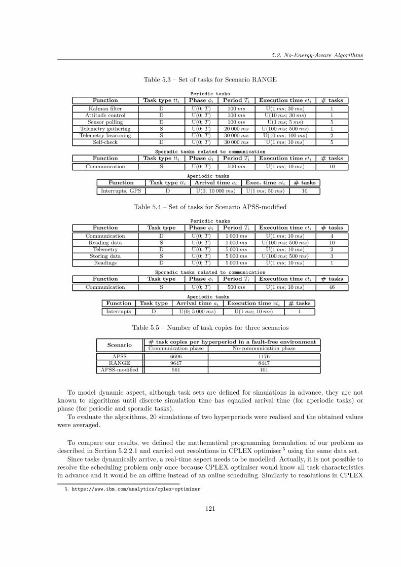
5.2. No-Energy-Aware Algorithms

Table 5.3 – Set of tasks for Scenario RANGE

Periodic tasks

Function Task type tti Phase φi Period Ti Execution time eti # tasks

Kalman filter D U(0; T ) 100 ms U(1 ms; 30 ms) 1Attitude control D U(0; T ) 100 ms U(10 ms; 30 ms) 1Sensor polling D U(0; T ) 100 ms U(1 ms; 5 ms) 5

Telemetry gathering S U(0; T ) 20 000 ms U(100 ms; 500 ms) 1Telemetry beaconing S U(0; T ) 30 000 ms U(10 ms; 100 ms) 2

Self-check D U(0; T ) 30 000 ms U(1 ms; 10 ms) 5

Sporadic tasks related to communication

Function Task type tti Phase φi Period Ti Execution time eti # tasks

Communication S U(0; T ) 500 ms U(1 ms; 10 ms) 10

Aperiodic tasks

Function Task type tti Arrival time ai Exec. time eti # tasks

Interrupts, GPS D U(0; 10 000 ms) U(1 ms; 50 ms) 10

Table 5.4 – Set of tasks for Scenario APSS-modified

Periodic tasks

Function Task type Phase φi Period Ti Execution time eti # tasks

Communication D U(0; T ) 1 000 ms U(1 ms; 10 ms) 4Reading data S U(0; T ) 1 000 ms U(100 ms; 500 ms) 10

Telemetry D U(0; T ) 5 000 ms U(1 ms; 10 ms) 2Storing data S U(0; T ) 5 000 ms U(100 ms; 500 ms) 3

Readings D U(0; T ) 5 000 ms U(1 ms; 10 ms) 1

Sporadic tasks related to communication

Function Task type Phase φi Period Ti Execution time eti # tasks

Communication S U(0; T ) 500 ms U(1 ms; 10 ms) 46

Aperiodic tasks

Function Task type Arrival time ai Execution time eti # tasks

Interrupts D U(0; 5 000 ms) U(1 ms; 10 ms) 1

Table 5.5 – Number of task copies for three scenarios

Scenario# task copies per hyperperiod in a fault-free environmentCommunication phase No-communication phase

APSS 6696 1176RANGE 9647 8447

APSS-modified 561 101

To model dynamic aspect, although task sets are defined for simulations in advance, they are notknown to algorithms until discrete simulation time has equalled arrival time (for aperiodic tasks) orphase (for periodic and sporadic tasks).

To evaluate the algorithms, 20 simulations of two hyperperiods were realised and the obtained valueswere averaged.

To compare our results, we defined the mathematical programming formulation of our problem asdescribed in Section 5.2.2.1 and carried out resolutions in CPLEX optimiser 5 using the same data set.

Since tasks dynamically arrive, a real-time aspect needs to be modelled. Actually, it is not possible toresolve the scheduling problem only once because CPLEX optimiser would know all task characteristicsin advance and it would be an offline instead of an online scheduling. Similarly to resolutions in CPLEX

5. https://www.ibm.com/analytics/cplex-optimizer

121

Chapter 5 – Online Fault Tolerant Scheduling Algorithms for CubeSats

solver described in Section 3.1.2.1, at each scheduling trigger, the main function updates task data(arrival/withdrawal of periodic task and/or arrival of aperiodic task) and launches a new resolution usingthe current data set.

Due to computational time constraints related to the dynamic task arrival of aperiodic tasks, onlyresults for OneOff&Cyclic were obtained. Actually, OneOff have many scheduling triggers, whichmake resolutions unfeasible within the reasonable time.

Fault Generation

For simulations with fault injection, we take into account that the worst estimated fault rate in thereal space environment is 10−5 fault/ms [118]. We therefore inject faults at the level of task copies withfault rate for each processor between 1 · 10−5 and 1 · 10−3 fault/ms in order to assess the algorithmperformances not only using the real fault rate but also its higher values. For the sake of simplicity, weconsider only transient faults and that one fault can impact at most one task copy.

Several curves are based on less than 20 simulations due to computational constraints. During thecommunication phase for systems consisting of 9 or 10 processors and OneOff&Cyclic at 1 · 10−3

fault/ms, there are no results due to hard computational time constraints. Actually, even 150 hours,which corresponds to the maximum possible computation time available on the computing grid on whichsimulations were carried out, was not sufficient for one simulation to be finished.

5.2.3.2 Metrics

We make use of the rejection rate, which is the ratio of rejected tasks to all arriving tasks, and thesystem throughput, which counts the number of correctly executed tasks. In a fault-free environment, thismetric is equal to the number of tasks minus the number of rejected tasks. The processor load is alsostudied to evaluate the processor utilisation.

To analyse the algorithm run-time, we use the following metrics. The task queue length stands for thenumber of tasks in the task queue, which are about to be ordered and scheduled. The algorithm run-timeis measured by the scheduling time, which is the time elapsed during one scheduling search. Finally, weevaluate the number of scheduling searches, i.e. how many times a search for a new schedule was carriedout.

5.2.4 Results

In this section, we first estimate the theoretical processor load and the proportion of simple and doubletasks in each scenarios. Then, we compare the rejection rate, analyse the number of scheduling searchesand scheduling times. Finally, we evaluate the algorithm performances in the presence of faults.

5.2.4.1 Theoretical Processor Load

In this section, we focus on the processor load and task proportions for each scenario in a fault-freeenvironment.

Based on Tables 5.2, 5.3 and 5.4, we compute the theoretical processor load when considering bothmaximum and mean execution times of each task. The results for three scenarios are depicted in Fig-ures 5.6 representing such processor loads respectively for both communication phases as a function ofthe number of processors.

Scenario RANGE has lower theoretical processor load than other two scenarios no matter the commu-nication phase. Theoretically, it means that all tasks for Scenario RANGE can be scheduled (maximumtheoretical processor load is between 22% for 10-processor systems and 82% for 3-processor systems)while it is not always possible for other two scenarios (APSS and APSS-modified) because the maximumtheoretical processor load exceeds 100% when a CubeSat has only a few processors.

Regarding the proportion of simple and double tasks, they are represented in Figures 5.7. It canbe observed that during the communication phase the percentage of double tasks for Scenarios APSS

122

5.2. No-Energy-Aware Algorithms

3 4 5 6 7 8 9 10Number of processors

0.2

0.4

0.6

0.8

1.0

1.2

Theo

retical processor load

for m

ean execution tim

e

Scenario APSSScenario RANGEScenario APSS-modified

(a) Mean et; Communication phase

3 4 5 6 7 8 9 10Number of processors

0.2

0.4

0.6

0.8

1.0

Theo

retical processor load

for m

ean execution tim

e

Scenario APSSScenario RANGEScenario APSS-modified

(b) Mean et; No-communication phase

3 4 5 6 7 8 9 10Number of processors

0.25

0.50

0.75

1.00

1.25

1.50

1.75

2.00

Theo

retical processor load

for m

axim

um executio

n tim

e Scenario APSSScenario RANGEScenario APSS-modified

(c) Maximum et; Communication phase

3 4 5 6 7 8 9 10Number of processors

0.2

0.4

0.6

0.8

1.0

1.2

1.4

1.6

1.8

Theo

retical processor load

for m

axim

um executio

n tim

e Scenario APSSScenario RANGEScenario APSS-modified

(d) Maximum et; No-communicationphase

Figure 5.6 – Theoretical processor load when considering maximum and mean execution times (et) ofeach task

APSS RANGE APSS-modifiedScenario

0.0

0.2

0.4

0.6

0.8

1.0

Prop

ortio

n

Double tasksSimple tasks

(a) Communication phase

APSS RANGE APSS-modifiedScenario

0.0

0.2

0.4

0.6

0.8

1.0

Prop

ortio

n

Double tasksSimple tasks

(b) No-communication phase

Figure 5.7 – Proportion of simple and double tasks

and APSS-modified is low (about 4%), while the task set for Scenario RANGE consists of 78% doubletasks. During the no-communication phase, the percentage of simple tasks is almost negligible (0.02%)for Scenario RANGE and it is about 30% for other two scenarios.

To conclude, our experimental framework makes use of two very different sets of scenarios. On theone hand, Scenarios APSS and APSS-modified have high system load and high proportion of simple taskscompared to double tasks. On the other hand, Scenario RANGE mainly contains double tasks and haslower system load.

5.2.4.2 Rejection Rate of OneOff and OneOff&Cyclic

We analyse the performances of OneOff and OneOff&Cyclic in terms of the rejection rate. Wecompare different ordering policies, listed in Section 5.2.2, for three scenarios in order to choose which

123

Chapter 5 – Online Fault Tolerant Scheduling Algorithms for CubeSats

ordering policy is the best in terms of the rejection rate. When an ordering policy is mentioned in thelegend it means that it is exclusively used by the algorithm and no other ordering policy is considered,whereas "All techniques" signifies that all ordering policies were tested to find a schedule.

Analysis of OneOff We compare different scenarios when OneOff is implemented. Figures 5.8 and5.9 respectively show the rejection rate of three scenarios for both communication and no-communicationphases as a function of the number of processors. First of all, it can be seen that Scenario RANGEhas almost no rejection rate during the communication phase and none rejection rate during the no-communication phase. This is due to the task data set, which has rather low system load as it wasaforementioned.

3 4 5 6 7 8 9 10Number of processors

0.0

0.1

0.2

0.3

0.4

0.5

0.6

0.7

Rejection rate

All techniquesMSHighest ratio et/(d-t)Lowest ratio et/(d-t)LETSETEATEDRandom

(a) Scenario APSS

3 4 5 6 7 8 9 10Number of processors

0.0000000

0.0000025

0.0000050

0.0000075

0.0000100

0.0000125

0.0000150

0.0000175

Rejection rate

All techniquesMSHighest ratio et/(d-t)Lowest ratio et/(d-t)LETSETEATEDRandom

(b) Scenario RANGE

3 4 5 6 7 8 9 10Number of processors

0.0

0.1

0.2

0.3

0.4

0.5

Rejection rate

All techniquesMSHighest ratio et/(d-t)Lowest ratio et/(d-t)LETSETEATEDRandom

(c) Scenario APSS-modified

Figure 5.8 – Rejection rate as a function of the number of processors (OneOff; communication phase)

3 4 5 6 7 8 9 10Number of processors

0.00

0.05

0.10

0.15

0.20

0.25

0.30

0.35

Rejection rate

All techniquesMSHighest ratio et/(d-t)Lowest ratio et/(d-t)LETSETEATEDRandom

(a) Scenario APSS

3 4 5 6 7 8 9 10Number of processors

0.00

0.01

0.02

0.03

0.04

0.05

Rejection rate

All techniquesMSHighest ratio et/(d-t)Lowest ratio et/(d-t)LETSETEATEDRandom

(b) Scenario RANGE

3 4 5 6 7 8 9 10Number of processors

0.00

0.02

0.04

0.06

0.08

0.10

Rejection rate

All techniquesMSHighest ratio et/(d-t)Lowest ratio et/(d-t)LETSETEATEDRandom

(c) Scenario APSS-modified

Figure 5.9 – Rejection rate as a function of the number of processors (OneOff; no-communication phase)

The "Earliest Deadline" or "Earliest Arrival Time" techniques overall reject the least tasks and "Alltechniques" does not achieve the lowest rejection rate all the time. To further evaluate the method "Alltechniques", Figures 5.10 depicts the number of victories among all tested ordering policies for bothcommunication phases. When several ordering policies achieve the same rejection rate, the algorithmchooses the schedule delivered by the first ordering policy in the list. As it can be seen in Figures 5.10,this is often the case when the system consists of more than five processors. In addition, when the numberof processors is low, the schedule delivered by the "Earliest Deadline" is chosen, even though this orderingpolicy is penultimate in the list of tested ordering policies. Consequently, the method "All techniques" willno longer be considered because its performances do not excel and it increases the algorithm run-timesince several ordering policies need to be tested, as stated in Algorithm 13 (Line 13).

Analysis of OneOff&Cyclic We contrast different scenarios when OneOff&Cyclic is used. Fig-ures 5.11 and 5.12 respectively depict the rejection rate of three scenarios for both communication and

124

5.2. No-Energy-Aware Algorithms

3 4 5 6 7 8 9 10Number of processors

0

2000

4000

6000

8000

10000

12000

Number o

f victories MS

Highest ratio et/(d-t)Lowest ratio et/(d-t)LETSETEATEDRandom

(a) Communication phase

3 4 5 6 7 8 9 10Number of processors

0250500750

1000125015001750

Number o

f victories MS

Highest ratio et/(d-t)Lowest ratio et/(d-t)LETSETEATEDRandom

(b) No-communication phase

Figure 5.10 – Number of victories for "All techniques" method as a function of the number of processors(OneOff; Scenario APSS)

no-communication phases as a function of the number of processors. These figures depict not only thestudied ordering policies and their combination, but also a curve plotting the optimal solution providedby CPLEX solver that is based on the mathematical programming formulation defined in Section 5.2.2.1.In general, the algorithm using the ordering policy achieving the lowest rejection rate has its competi-tive ratio of 2 or 3, which are rather good results taking into account that our search is not exhaustivecompared to the search for the optimal solution.

3 4 5 6 7 8 9 10Number of processors

0.0

0.1

0.2

0.3

0.4

Rejection rate

CPLEX solutionsAll techniquesHighest ratio et/(d-t)Lowest ratio et/(d-t)MSLETSETEPRMRandom

(a) Scenario APSS

3 4 5 6 7 8 9 10Number of processors

0.00

0.01

0.02

0.03

0.04

0.05

0.06

Rejection rate

CPLEX solutionsAll techniquesHighest ratio et/(d-t)Lowest ratio et/(d-t)MSLETSETEPRMRandom

(b) Scenario RANGE

3 4 5 6 7 8 9 10Number of processors

0.0

0.1

0.2

0.3

0.4

Rejection rate

CPLEX solutionsAll techniquesHighest ratio et/(d-t)Lowest ratio et/(d-t)MSLETSETEPRMRandom

(c) Scenario APSS-modified

Figure 5.11 – Rejection rate as a function of the number of processors (OneOff&Cyclic; communicationphase)

3 4 5 6 7 8 9 10Number of processors

0.00

0.05

0.10

0.15

0.20

0.25

0.30

Rejection rate

CPLEX solutionsAll techniquesHighest ratio et/(d-t)Lowest ratio et/(d-t)MSLETSETEPRMRandom

(a) Scenario APSS

3 4 5 6 7 8 9 10Number of processors

0.000

0.005

0.010

0.015

0.020

0.025

0.030

Rejection rate

CPLEX solutionsAll techniquesHighest ratio et/(d-t)Lowest ratio et/(d-t)MSLETSETEPRMRandom

(b) Scenario RANGE

3 4 5 6 7 8 9 10Number of processors

0.00

0.05

0.10

0.15

0.20

0.25

0.30

Rejection rate

CPLEX solutionsAll techniquesHighest ratio et/(d-t)Lowest ratio et/(d-t)MSLETSETEPRMRandom

(c) Scenario APSS-modified

Figure 5.12 – Rejection rate as a function of the number of processors (OneOff&Cyclic; no-communication phase)

Again, Scenario RANGE has several times lower rejection rate than other two scenarios because of

125

Chapter 5 – Online Fault Tolerant Scheduling Algorithms for CubeSats

lower system load. Furthermore, it can be seen that it is not so straightforward to determine one orderingpolicy, which performs well for all scenarios. Although the method "All techniques", testing all orderingpolicies reject the least tasks, it will not be considered any more due to longer algorithm run-time. Thus, areasonable choice is the "Minimum Slack" or "Earliest Phase" techniques during the communication phaseand the "Minimum Slack" or "Longest Execution Time" during the no-communication phase. Altogether,the "Minimum Slack" ordering policy perform well regardless of the type of phase. Nevertheless, therejection rate of OneOff&Cyclic is in general higher than the one of OneOff.

Comparison of Different Scenarios The performances of a given ordering policy are influencedby the system load and task proportions. The influence of the former factor is illustrated by ScenarioRANGE, which has much lower (or none) rejection rate than other two scenarios.

The impact of the latter factor is demonstrated by the difference of rejection rates for Scenarios APSSand APSS-modified. For several ordering policies, the rejection rate is higher during the no-communicationphase than during the communication one despite the fact that there are less tasks during the no-communication phase. Actually, there are 29.4% double tasks during the no-communication phase against4.2% double tasks during the communication phase. To illustrate this difference, Figures 5.13 show theproportion of simple and double tasks against the rejection rate for Scenario APSS as a function of thenumber of processors when OneOff using the "Earliest Deadline" policy is put into practice.

3 4 5 6 7 8 9 10Number of processors

0.0

0.2

0.4

0.6

0.8

1.0

Percen

tage

(a) Communication phase

3 4 5 6 7 8 9 10Number of processors

0.0

0.2

0.4

0.6

0.8

1.0

Percen

tage

(b) No-communication phase

Figure 5.13 – Proportion of simple and double tasks against the rejection rate as a function of the numberof processors (OneOff using the "Earliest Deadline" policy; Scenario APSS)

In order not to oversize the system, the analysis of the rejection rate (regardless of the scenario) alsoshows that it is useless to consider more than six processors. In fact, when an ordering policy is wellchosen, no task is rejected.

5.2.4.3 Number of Scheduling Searches

In this section, we compare the number of scheduling searches, i.e. how many times a search fora new schedule was carried out. We consider the "Earliest Deadline" ordering policy when analysingOneOff and the "Minimum Slack" policy for OneOff&Cyclic because it was shown in Section 5.2.4.2that they achieve the best results in terms of the number of rejected tasks. Figures 5.14 depict thenumber of scheduling searches for three CubeSat scenarios for both studied algorithm, OneOff andOneOff&Cyclic.

Figures 5.14 point out that the number of scheduling searches of OneOff is significantly higher whencompared to OneOff&Cyclic.

As defined in Formula 5.2, the former algorithm (OneOff) has the number of scheduling searches atmost equal to the sum of the number of tasks to be scheduled and the number of task copies. In general,the number of scheduling searches is lower than the maximum theoretical value and approximately equalsthe number of tasks at the input when there are more processors in the system because every task activates

126

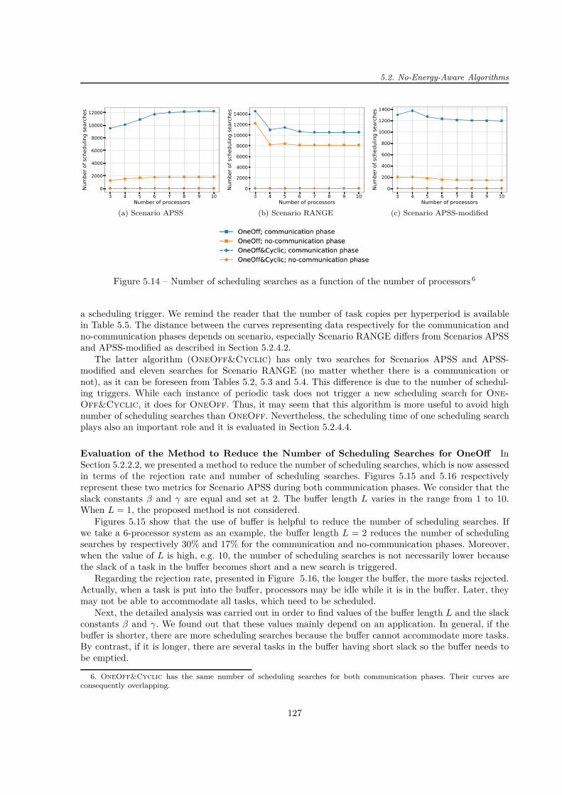
5.2. No-Energy-Aware Algorithms

3 4 5 6 7 8 9 10Number of processors

0

2000

4000

6000

8000

10000

12000

Numbe

r of s

ched

uling search

es

(a) Scenario APSS

3 4 5 6 7 8 9 10Number of processors

0

2000

4000

6000

8000

10000

12000

14000

Numbe

r of s

ched

uling search

es

(b) Scenario RANGE

3 4 5 6 7 8 9 10Number of processors

0

200

400

600

800

1000

1200

1400

Numbe

r of s

ched

uling search

es

(c) Scenario APSS-modified

Figure 5.14 – Number of scheduling searches as a function of the number of processors 6

a scheduling trigger. We remind the reader that the number of task copies per hyperperiod is availablein Table 5.5. The distance between the curves representing data respectively for the communication andno-communication phases depends on scenario, especially Scenario RANGE differs from Scenarios APSSand APSS-modified as described in Section 5.2.4.2.

The latter algorithm (OneOff&Cyclic) has only two searches for Scenarios APSS and APSS-modified and eleven searches for Scenario RANGE (no matter whether there is a communication ornot), as it can be foreseen from Tables 5.2, 5.3 and 5.4. This difference is due to the number of schedul-ing triggers. While each instance of periodic task does not trigger a new scheduling search for One-Off&Cyclic, it does for OneOff. Thus, it may seem that this algorithm is more useful to avoid highnumber of scheduling searches than OneOff. Nevertheless, the scheduling time of one scheduling searchplays also an important role and it is evaluated in Section 5.2.4.4.

Evaluation of the Method to Reduce the Number of Scheduling Searches for OneOff InSection 5.2.2.2, we presented a method to reduce the number of scheduling searches, which is now assessedin terms of the rejection rate and number of scheduling searches. Figures 5.15 and 5.16 respectivelyrepresent these two metrics for Scenario APSS during both communication phases. We consider that theslack constants β and γ are equal and set at 2. The buffer length L varies in the range from 1 to 10.When L = 1, the proposed method is not considered.

Figures 5.15 show that the use of buffer is helpful to reduce the number of scheduling searches. Ifwe take a 6-processor system as an example, the buffer length L = 2 reduces the number of schedulingsearches by respectively 30% and 17% for the communication and no-communication phases. Moreover,when the value of L is high, e.g. 10, the number of scheduling searches is not necessarily lower becausethe slack of a task in the buffer becomes short and a new search is triggered.

Regarding the rejection rate, presented in Figure 5.16, the longer the buffer, the more tasks rejected.Actually, when a task is put into the buffer, processors may be idle while it is in the buffer. Later, theymay not be able to accommodate all tasks, which need to be scheduled.

Next, the detailed analysis was carried out in order to find values of the buffer length L and the slackconstants β and γ. We found out that these values mainly depend on an application. In general, if thebuffer is shorter, there are more scheduling searches because the buffer cannot accommodate more tasks.By contrast, if it is longer, there are several tasks in the buffer having short slack so the buffer needs tobe emptied.

6. OneOff&Cyclic has the same number of scheduling searches for both communication phases. Their curves areconsequently overlapping.

127

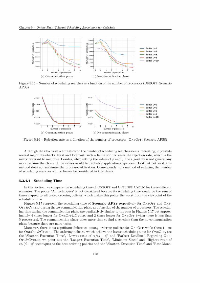
Chapter 5 – Online Fault Tolerant Scheduling Algorithms for CubeSats

3 4 5 6 7 8 9 10Number of processors

4000

6000

8000

10000

12000

14000

Numbe

r of s

ched

uling

(a) Communication phase

3 4 5 6 7 8 9 10Number of processors

1200

1400

1600

1800

2000

2200

2400

2600

Numbe

r of s

ched

uling

(b) No-communication phase

Figure 5.15 – Number of scheduling searches as a function of the number of processors (OneOff; ScenarioAPSS)

3 4 5 6 7 8 9 10Number of processors

0.000

0.005

0.010

0.015

0.020

Rejection rate

(a) Communication phase

3 4 5 6 7 8 9 10Number of processors

0.00

0.05

0.10

0.15

0.20

Rejection rate

(b) No-communication phase

Figure 5.16 – Rejection rate as a function of the number of processors (OneOff; Scenario APSS)

Although the idea to set a limitation on the number of scheduling searches seems interesting, it presentsseveral major drawbacks. First and foremost, such a limitation increases the rejection rate, which is themetric we want to minimise. Besides, when setting the values of β and γ, the algorithm is not general anymore because the choice of the values would be probably application-dependent. Last but not least, thismethod does not maximise the processor utilisation. Consequently, this method of reducing the numberof scheduling searches will no longer be considered in this thesis.

5.2.4.4 Scheduling Time

In this section, we compare the scheduling time of OneOff and OneOff&Cyclic for three differentscenarios. The policy "All techniques" is not considered because its scheduling time would be the sum oftimes elapsed by all tested ordering policies, which makes this policy the worst from the viewpoint of thescheduling time.

Figures 5.17 represent the scheduling time of Scenario APSS respectively for OneOff and One-Off&Cyclic during the no-communication phase as a function of the number of processors. The schedul-ing time during the communication phase are qualitatively similar to the ones in Figures 5.17 but approx-imately 4 times longer for OneOff&Cyclic and 2 times longer for OneOff (when there is less than5 processors). The communication phase takes more time to find a schedule than the no-communicationphase because there are more tasks.

Moreover, there is no significant difference among ordering policies for OneOff while there is onefor OneOff&Cyclic. The ordering policies, which achieve the lowest scheduling time for OneOff, arethe "Shortest Execution Time", "Lowest ratio of et/(d − t)" and "Earliest Deadline". Regarding One-Off&Cyclic, we point out the "Longest Execution Time", "Minimum Slack" and "Highest ratio ofet/(d − t)" techniques as the best ordering policies and the "Shortest Execution Time" and "Rate Mono-

128

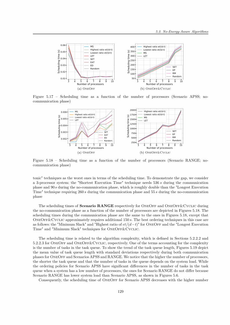
5.2. No-Energy-Aware Algorithms

3 4 5 6 7 8 9 10Number of processors

0.01

0.02

0.03

0.04

0.05

0.06

Scheduling tim

e (s)

MSHighest ratio et/(d-t)Lowest ratio et/(d-t)LETSETEATEDRandom

(a) OneOff

3 4 5 6 7 8 9 10Number of processors

50100150200250300350400

Sche

dulin

g tim

e (s

)

Highest ratio et/(d-t)Lowest ratio et/(d-t)MSLET

SETEPRMRandom

SETEPRMRandom

(b) OneOff&Cyclic

Figure 5.17 – Scheduling time as a function of the number of processors (Scenario APSS; no-communication phase)

3 4 5 6 7 8 9 10Number of processors

0.002

0.003

0.004

0.005

0.006

Scheduling tim

e (s)

MSHighest ratio et/(d-t)Lowest ratio et/(d-t)LET

SETEATEDRandom

SETEATEDRandom

(a) OneOff

3 4 5 6 7 8 9 10Number of processors

250

500

750

1000

1250

1500

1750

2000

Sche

dulin

g tim

e (s

)

Highest ratio et/(d-t)Lowest ratio et/(d-t)MSLET

SETEPRMRandom

SETEPRMRandom

(b) OneOff&Cyclic

Figure 5.18 – Scheduling time as a function of the number of processors (Scenario RANGE; no-communication phase)

tonic" techniques as the worst ones in terms of the scheduling time. To demonstrate the gap, we considera 3-processor system: the "Shortest Execution Time" technique needs 536 s during the communicationphase and 90s during the no-communication phase, which is roughly double than the "Longest ExecutionTime" technique requiring 260 s during the communication phase and 55 s during the no-communicationphase

The scheduling times of Scenario RANGE respectively for OneOff and OneOff&Cyclic duringthe no-communication phase as a function of the number of processors are depicted in Figures 5.18. Thescheduling times during the communication phase are the same to the ones in Figures 5.18, except thatOneOff&Cyclic approximately requires additional 150 s. The best ordering techniques in this case areas follows: the "Minimum Slack" and "Highest ratio of et/(d−t)" for OneOff and the "Longest ExecutionTime" and "Minimum Slack" techniques for OneOff&Cyclic.

The scheduling time is related to the algorithm complexity, which is defined in Sections 5.2.2.2 and5.2.2.3 for OneOff and OneOff&Cyclic, respectively. One of the terms accounting for the complexityis the number of tasks in the task queue. To show the trend of the task queue length, Figures 5.19 depictthe mean value of task queue length with standard deviations respectively during both communicationphases for OneOff and Scenarios APSS and RANGE. We notice that the higher the number of processors,the shorter the task queue and that the number of tasks in the queue depends on the system load. Whilethe ordering policies for Scenario APSS have significant differences in the number of tasks in the taskqueue when a system has a low number of processors, the ones for Scenario RANGE do not differ becauseScenario RANGE has lower system load than Scenario APSS, as shown in Figures 5.6.

Consequently, the scheduling time of OneOff for Scenario APSS decreases with the higher number

129

Chapter 5 – Online Fault Tolerant Scheduling Algorithms for CubeSats

3 4 5 6 7 8 9 10Number of processors

0

20

40

60

80

100

120

Mea

n of ta

sk que

ue le

ngth

(a) Scenario APSS;Communication phase

3 4 5 6 7 8 9 10Number of processors

0

5

10

15

20

25

30

35

Mea

n of ta

sk que

ue le

ngth

(b) Scenario APSS;No-communication phase

3 4 5 6 7 8 9 10Number of processors

1.5

2.0

2.5

3.0

3.5

Mea

n of ta

sk que

ue le

ngth

(d) Scenario RANGE;Communication phase

3 4 5 6 7 8 9 10Number of processors

1.752.002.252.502.753.003.253.50

Mea

n of ta

sk que

ue le

ngth

(e) Scenario RANGE;No-communication phase

Figure 5.19 – Mean value of task queue length with standard deviations as a function of the number ofprocessors (OneOff)

of processors owing to shorter task queue because there are more scheduling triggers. Regarding thescheduling time of OneOff&Cyclic, it is longer when the number of processors increases even thoughthe number of tasks is almost constant (the set of periodic tasks remains the same for a given phase andthere is only one (Scenario APSS) or ten (Scenario RANGE) arrivals of aperiodic tasks). The increase isdue to more possibilities to be tested when a system has more processors.

Nonetheless, as the results are based on simulations (because real experiments are not easily feasible),scheduling times in our experiments do not significantly change as the task queue length could foresee.This difference is due to the additional complexity related to our simulation framework (handling ofarrays in time standing for schedules on processors), which will not be present in reality and the realscheduling times will be shorter.

Last but not least, the scheduling time of OneOff&Cyclic is roughly 5 orders of magnitude greaterthan the one of OneOff. This huge gap is mainly caused by the significant difference in task periods:between 500 ms and 60 000 ms. To better evaluate this impact on scheduling time, we modified ScenarioAPSS to Scenario APSS-modified, as described in Section 5.2.3.1.

Figures 5.20 represent the scheduling time of Scenario APSS-modified respectively for OneOffand OneOff&Cyclic during the no-communication phase as a function of the number of processors.The trend of scheduling times during the communication phase is similar to the ones in Figures 5.20 andthe values are multiplied by a number within the range from 5 to 10 for OneOff&Cyclic and by 2 forOneOff (when a system has less than 6 processors).

The scheduling time of OneOff&Cyclic is roughly 3 orders of magnitude greater than the one ofOneOff. We conclude that the idea to reduce the substantial difference in task periods accelerates thescheduling time. We therefore suggest to teams building CubeSats to avoid tasks with very short andvery long periods to be scheduled together.

130

5.2. No-Energy-Aware Algorithms

3 4 5 6 7 8 9 10Number of processors

0.0004

0.0006

0.0008

0.0010

0.0012

0.0014

Schedu

ling tim

e (s)

Highest ratio et/(d-t)Lowest ratio et/(d-t)

MSLETSETEPRMRandom

MSLETSETEPRMRandom

(a) OneOff

3 4 5 6 7 8 9 10Number of processors

0.75

1.00

1.25

1.50

1.75

2.00

2.25

Schedu

ling tim

e (s)

Highest ratio et/(d-t)Lowest ratio et/(d-t)MSLET

SETEPRMRandom

SETEPRMRandom

(b) OneOff&Cyclic

Figure 5.20 – Scheduling time as a function of the number of processors (Scenario APSS-modified; no-communication phase)

5.2.4.5 Simulations with Fault Injection

In this section, we evaluate the fault tolerance of both algorithms for Scenario APSS. We chose thisscenario because it is based on real data (and not on a modified version) and it has rather high systemload when compared to Scenario RANGE. We consider the "Earliest Deadline" policy for OneOff andthe "Minimum Slack" policy for OneOff&Cyclic.

3 4 5 6 7 8 9 10Number of processors

0

2

4

6

8

10

12

Number

Faults without impactFaults impacting simple tasksFaults impacting double tasks

(a) Communication phase

3 4 5 6 7 8 9 10Number of processors

0

2

4

6

8

10

12

Number

Faults without impactFaults impacting simple tasksFaults impacting double tasks

(b) No-communication phase

Figure 5.21 – Total number of faults (injected with fault rate 1 · 10−5 fault/ms) against the number ofprocessors (OneOff; Scenario APSS)

Figures 5.21 depict the total number of faults against the number of processors, while the total numberis the sum of the faults without impact, faults impacting simple tasks and faults impacting double tasks.The fault were injected with fault rate 1 · 10−5 fault/ms, which corresponds to the worst estimatedfault rate in the real space environment [118]. Albeit only values for OneOff are shown, the ones forOneOff&Cyclic are similar. We remind the reader that presented results were computed as an averageof 20 simulations and they consequently may not be integers.

The number of impacted tasks remains almost constant and there is no significant difference betweentwo algorithms nor between communication phases. Furthermore, double tasks are rarely impacted, whichis due to their shorter execution time compared with simple tasks. We also studied other fault rates and,as expected, the higher the fault rate, the more faults. Nonetheless, the proportion of impacted simpleand double tasks remains the same.

Figures 5.22 and 5.23 respectively depict the rejection rate, system throughput and processor load forboth communication phases as a function of the number of processors. Qualitatively similar results wereobtained for OneOff&Cyclic. The figures representing the system throughput include a black dashedline corresponding to the case when no task is rejected and all tasks are correctly executed. Regardingthe figures plotting the processor load, they also show a black dashed line, which denotes the maximum

131

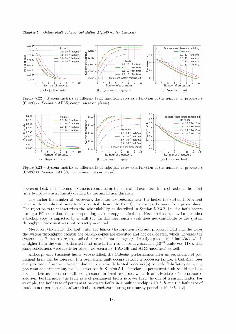
Chapter 5 – Online Fault Tolerant Scheduling Algorithms for CubeSats

3 4 5 6 7 8 9 10Number of processors

0.000

0.005

0.010

0.015

0.020

0.025

0.030

0.035

Reje

ctio

n ra

te

No fault1.0 10−5 fault/ms1.0 10−4 fault/ms5.0 10−4 fault/ms1.0 10−3 fault/ms

(a) Rejection rate

3 4 5 6 7 8 9 10Number of processors

12400

12500

12600

12700

12800

System

throug

hput

No faults1.0 ⋅ 10−5 fault/ms1.0 ⋅ 10−4 fault/ms5.0 ⋅ 10−4 fault/ms1.0 ⋅ 10−3 fault/ms

Ma imum system throughputMa imum system throughput

(b) System throughput

3 4 5 6 7 8 9 10Number of processors

0.4

0.6

0.8

1.0

1.2

Processor load

No fa lts1.0 ⋅ 10−5 fa lt/ms1.0 ⋅ 10−4 fa lt/ms5.0 ⋅ 10−4 fa lt/ms1.0 ⋅ 10−3 fa lt/ms

Processor load before sched lingProcessor load before sched ling

(c) Processor load

Figure 5.22 – System metrics at different fault injection rates as a function of the number of processors(OneOff; Scenario APSS; communication phase)

3 4 5 6 7 8 9 10Number of processors

0.0000.0250.0500.0750.1000.1250.1500.1750.200

Reje

ctio

n ra

te

No fault1.0 10−5 fault/ms1.0 10−4 fault/ms5.0 10−4 fault/ms1.0 10−3 fault/ms

(a) Rejection rate

3 4 5 6 7 8 9 10Number of processors

1400

1500

1600

1700

1800

S stem

throug

hput

No faults1.0 ⋅ 10−5 fault/ms1.0 ⋅ 10−4 fault/ms5.0 ⋅ 10−4 fault/ms1.0 ⋅ 10−3 fault/ms

Maximum s stem throughputMaximum s stem throughput

(b) System throughput

3 4 5 6 7 8 9 10Number of processors

0.30.40.50.60.70.80.91.01.1

Processor load

No faults1.0 ⋅ 10 5 fault/ms1.0 ⋅ 10 4 fault/ms5.0 ⋅ 10 4 fault/ms1.0 ⋅ 10 3 fault/ms

Processor load before schedulingProcessor load before scheduling

(c) Processor load

Figure 5.23 – System metrics at different fault injection rates as a function of the number of processors(OneOff; Scenario APSS; no-communication phase)

processor load. This maximum value is computed as the sum of all execution times of tasks at the input(in a fault-free environment) divided by the simulation duration.

The higher the number of processors, the lower the rejection rate, the higher the system throughputbecause the number of tasks to be executed aboard the CubeSat is always the same for a given phase.The rejection rate characterises the schedulability as described in Section 5.2.3.2, i.e. if a fault occursduring a PC execution, the corresponding backup copy is scheduled. Nevertheless, it may happen thata backup copy is impacted by a fault too. In this case, such a task does not contribute to the systemthroughput because it was not correctly executed.

Moreover, the higher the fault rate, the higher the rejection rate and processor load and the lowerthe system throughput because the backup copies are executed and not deallocated, which increases thesystem load. Furthermore, the studied metrics do not change significantly up to 1 · 10−4 fault/ms, whichis higher than the worst estimated fault rate in the real space environment (10−5 fault/ms [118]). Thesame conclusions were made for other two scenarios (RANGE and APSS-modified) as well.

Although only transient faults were studied, the CubeSat performances after an occurrence of per-manent fault can be foreseen. If a permanent fault occurs causing a processor failure, a CubeSat losesone processor. Since we consider that there are no dedicated processor(s) to each CubeSat system, anyprocessor can execute any task, as described in Section 5.1. Therefore, a permanent fault would not be aproblem because there are still enough computational resources, which is an advantage of the proposedsolution. Furthermore, the fault rate of permanent faults is lower than the one of transient faults. Forexample, the fault rate of permanent hardware faults in a multicore chip is 10−5/h and the fault rate ofrandom non-permanent hardware faults in each core during non-bursty period is 10−4/h [118].

132

5.3. Energy-Aware Algorithm

5.3 Energy-Aware Algorithm

The preceding section presented two algorithms for reduction in the rejection rate that are applicable toCubeSats. It was shown that OneOff, i.e. an online algorithm scheduling arriving tasks as the aperiodicones, achieves better results in terms of the rejection rate and scheduling time than OneOff&Cyclic,which is an online algorithm scheduling arriving tasks as the aperiodic or periodic ones. Therefore, weconsider onwards OneOff only. In this section, this algorithm is enhanced in the sense it also takes intoconsideration energy constraints because energy is of major interest for satellite applications.

5.3.1 System, Fault and Task Models

While the fault model is exactly the same as described in Section 5.2.1, the system and task modelsslightly differ.

Since OneOff is put into practice, all tasks are considered as aperiodic. Every task is characterised bythe arrival time ai, execution time eti, deadline di, task type tti and task priority tpi. The last attributetakes on three possible values: high (H), middle (M) and low (L), and it characterises the balance betweenthe task importance and energy consumption. For instance, the tasks related to CubeSat housekeepinghave higher priority than the tasks associated with payload. Similarly, while it is appropriate to send asignal that a CubeSat is still operating to the ground station during the communication phase in the caseit experiences the energy shortage, it may not be necessary to transmit all reports.

Since there are three task priorities, the system distinguishes three operating modes: normal (N),safe (S) and critical (C). Inspired by [14], the system chooses a mode according to the current batterycapacity. Table 5.6 associates each mode with the battery capacity and tasks that are authorised to beexecuted.

Table 5.6 – System operating modes

Mode Battery capacityExecuted tasks

Tasks having tpi = H Tasks having tpi = M Tasks having tpi = L

Normal 50% – 100% X X X

Safe 20% – 50% X X -

Critical 0% – 20% X - -

We consider that the system regularly harvests energy, e.g. from the sun, stored in a battery andconsumes it to power processors. Although the dynamic voltage and frequency scaling may be availablewhen executing tasks, we do not make use of it because it does not improve the reliability, as discussedin Section 1.5. All tasks are thereby always executed at the maximum processor frequency.

Without loss of generality, we take an example of STM32F103 processor based on ARM 32-bit Cortex-M3 CPU because it is commonly used on board of CubeSats, as shown in Table 4.2. Its characteristics forthe maximum (72 MHz) and minimum (125 kHz) frequencies and four operating modes are summarisedin Table 5.7.

Table 5.7 – Several characteristics of STM32F103 processor

Operating mode IDD VDD PST M32F 103 Wakeup time

Run (72 MHz) 52.5 mA 3.3 V 173 mW 0 µs

Run (125 kHz) 1.4 mA 3.3 V 4.6 mW 0 µs

Sleep (72 MHz) 32.5 mA 3.3 V 107 mW 1.8 µs

Sleep (125 kHz) 1.35 mA 3.3 V 4.5 mW 1.8 µs

Stop 38.7 µA 3.3 V 0.13 mW 5.4 µs

Standby 2.5 µA 3.3 V 0.0083 mW 50 µs

133

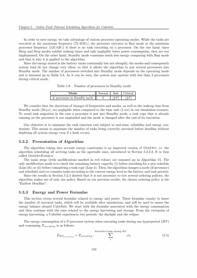
Chapter 5 – Online Fault Tolerant Scheduling Algorithms for CubeSats

In order to save energy, we take advantage of various processor operating modes. While the tasks areexecuted at the maximum frequency (72 MHz), the processor executes in Run mode at the minimumprocessor frequency (125 kHz) if there is no task executing on a processor. On the one hand, sinceSleep and Stop modes exhibit wakeup times and only negligibly lower power consumption, they are notimplemented. On the other hand, Standby mode consumes much less energy comparing with Run modeand that is why it is applied to the algorithm.

Since the energy stored in the battery varies continually but not abruptly, the modes and consequentlysystem load do not change very often, so that it allows the algorithm to put several processors intoStandby mode. The number of processors switched into Standby mode depends on the operating modeand is summed up in Table 5.8. As it can be seen, the system may operate with less than 3 processorsduring critical mode.

Table 5.8 – Number of processors in Standby mode

Mode Normal Safe Critical

# processors in Standby mode 0 ⌊ 16P ⌋ ⌊ 1

3P ⌋

We consider that the durations of changes of frequencies and modes, as well as the wakeup time fromStandby mode (50 µs), are negligible when compared to the time unit (1 ms) in our simulation scenario.To avoid task migration in the case a processor is put into Standby mode, a task copy that is alreadyrunning on the processor is not suspended and the mode is changed after the end of its execution.

Our objective is to minimise the task rejection rate subject to real-time, reliability and energy con-straints. This means to maximise the number of tasks being correctly executed before deadline withoutdepleting all system energy even if a fault occurs.

5.3.2 Presentation of Algorithm

The algorithm taking into account energy constraints is an improved version of OneOff, i.e. thealgorithm scheduling all arriving tasks as the aperiodic ones, introduced in Section 5.2.2.2. It is thuscalled OneOffEnergy.

The main steps (with modifications marked in red colour) are summed up in Algorithm 15. Theonly modification made is to check the remaining battery capacity (i) before searching for a new schedule(Line 16), or (ii) before committing a task copy (Line 4). Then, the algorithm changes a mode (if necessary)and schedules and/or commits tasks according to the current energy level in the battery and task priority.

Since the results in Section 5.2.4 showed that it is not necessary to test several ordering policies, thealgorithm makes use of only one policy. Based on our previous results, the chosen ordering policy is the"Earliest Deadline".

5.3.3 Energy and Power Formulae

This section covers several formulae related to energy and power. These formulae require to knowthe number of executed tasks, which will be available after simulations, and will be used to assess theenergy balance aboard CubeSats. We start with the formulae associated with the energy consumptionand then continue with the ones related to the energy harvesting and storage. From the viewpoint ofenergy harvesting, a CubeSat experiences two periods: the daylight and the eclipse.

The energy consumption of a P -processor system when executing tasks during one hyperperiod (HT )and consuming Pexecuting is as follows:

EHTexecuting= Pexecuting ·

Scheduled tasks during HT∑

i

eti (5.5)

134

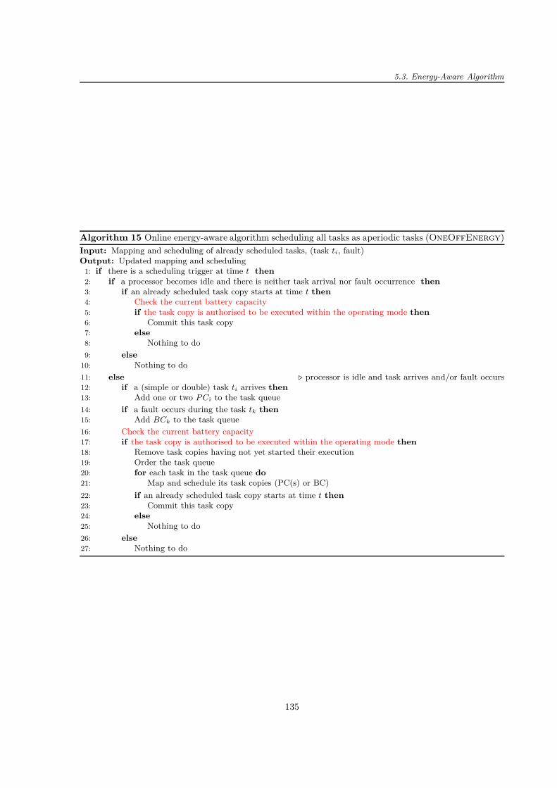
5.3. Energy-Aware Algorithm

Algorithm 15 Online energy-aware algorithm scheduling all tasks as aperiodic tasks (OneOffEnergy)Input: Mapping and scheduling of already scheduled tasks, (task ti, fault)Output: Updated mapping and scheduling

1: if there is a scheduling trigger at time t then2: if a processor becomes idle and there is neither task arrival nor fault occurrence then3: if an already scheduled task copy starts at time t then4: Check the current battery capacity5: if the task copy is authorised to be executed within the operating mode then6: Commit this task copy7: else8: Nothing to do

9: else10: Nothing to do

11: else ⊲ processor is idle and task arrives and/or fault occurs12: if a (simple or double) task ti arrives then13: Add one or two P Ci to the task queue

14: if a fault occurs during the task tk then15: Add BCk to the task queue

16: Check the current battery capacity17: if the task copy is authorised to be executed within the operating mode then18: Remove task copies having not yet started their execution19: Order the task queue20: for each task in the task queue do21: Map and schedule its task copies (PC(s) or BC)

22: if an already scheduled task copy starts at time t then23: Commit this task copy24: else25: Nothing to do

26: else27: Nothing to do

135

Chapter 5 – Online Fault Tolerant Scheduling Algorithms for CubeSats

The energy consumption of the P -processor system when idle during one hyperperiod (HT ) andconsuming Pidle is as reads:

EHTidle= Pidle ·

(

P · tHT −Scheduled tasks during HT

∑

i

eti

)

(5.6)

where tHT denotes the duration of one hyperperiod.Summing Formulae 5.5 and 5.6, we get the energy consumption of the P -processor system during one

hyperperiod (HT ):

EHT = EHTexecuting+ EHTidle

(5.7)

and we can assess the power of the system consisting of P processors based on the energy consumptionduring one hyperperiod:

Psystem =EHT

tHT(5.8)

If we consider that the energy is consumed not only by processors aboard CubeSats but also by othercomponents, such as a radio transmitter (TX) or a receiver (RX), the overall CubeSat power is as follows:

PCubeSat =CubeSat components

∑

i

Pi · (duty cycle) (5.9)

The value of PCubeSat depends on the operating mode chosen by the algorithm.

As regards the harvested power, we consider that a CubeSat has a solar panel delivering Pharvested.The power available to recharge the battery Pcharge is dependent on the current power consumptionPCubeSat [28]:

Pcharge = Pharvested · ηd − PCubeSat (5.10)

where ηd denotes the transmission efficiency from solar panel to load [35].The energy supplied by the solar panel during the daylight to charge the battery Esupplied is as follows

[28]:

Esupplied = Pcharge · (time spent in the daylight within one orbit) (5.11)

This energy can be compared to the energy needed during the eclipse to power the CubeSat [28]:

Eneeded =Pcharge · (time spent in the eclipse within one orbit)

ηe(5.12)

where ηe stands for the transmission efficiency from solar panel to battery and from battery to load [35].To compute the energy stored in the battery, we make use of the following formula [28]:

Ebattery = ηbattery · Vbattery · CAh · DOD (5.13)

where— ηbattery: battery transmission efficiency— DOD: depth of discharge 7

— Vbattery: battery voltage— CAh: battery capacity in Ah (battery capacity in Wh is computed as CW h = Vbattery · CAh)

7. Depth of Discharge (DOD) is the percentage of the capacity that has been removed from the fully charged battery[135].

136

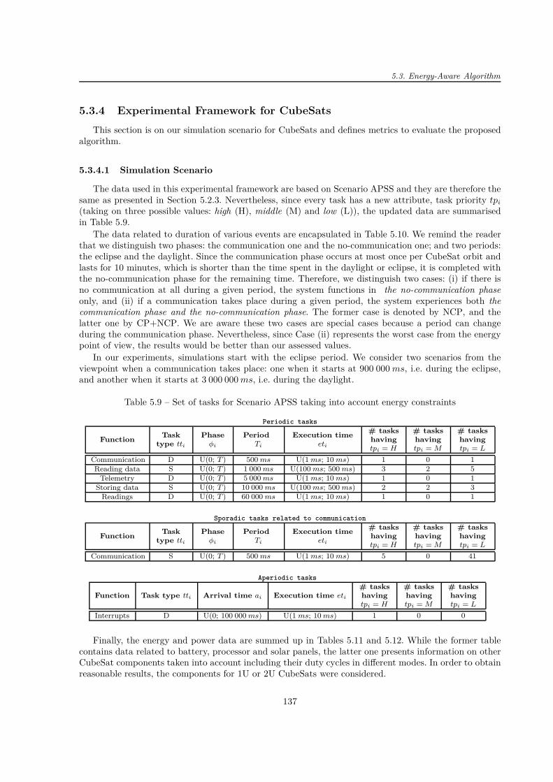
5.3. Energy-Aware Algorithm

5.3.4 Experimental Framework for CubeSats

This section is on our simulation scenario for CubeSats and defines metrics to evaluate the proposedalgorithm.

5.3.4.1 Simulation Scenario

The data used in this experimental framework are based on Scenario APSS and they are therefore thesame as presented in Section 5.2.3. Nevertheless, since every task has a new attribute, task priority tpi

(taking on three possible values: high (H), middle (M) and low (L)), the updated data are summarisedin Table 5.9.

The data related to duration of various events are encapsulated in Table 5.10. We remind the readerthat we distinguish two phases: the communication one and the no-communication one; and two periods:the eclipse and the daylight. Since the communication phase occurs at most once per CubeSat orbit andlasts for 10 minutes, which is shorter than the time spent in the daylight or eclipse, it is completed withthe no-communication phase for the remaining time. Therefore, we distinguish two cases: (i) if there isno communication at all during a given period, the system functions in the no-communication phaseonly, and (ii) if a communication takes place during a given period, the system experiences both thecommunication phase and the no-communication phase. The former case is denoted by NCP, and thelatter one by CP+NCP. We are aware these two cases are special cases because a period can changeduring the communication phase. Nevertheless, since Case (ii) represents the worst case from the energypoint of view, the results would be better than our assessed values.

In our experiments, simulations start with the eclipse period. We consider two scenarios from theviewpoint when a communication takes place: one when it starts at 900 000 ms, i.e. during the eclipse,and another when it starts at 3 000 000 ms, i.e. during the daylight.

Table 5.9 – Set of tasks for Scenario APSS taking into account energy constraints

Periodic tasks

FunctionTask

type tti

Phaseφi

PeriodTi

Execution timeeti

# taskshavingtpi = H

# taskshavingtpi = M

# taskshavingtpi = L

Communication D U(0; T ) 500 ms U(1 ms; 10 ms) 1 0 1

Reading data S U(0; T ) 1 000 ms U(100 ms; 500 ms) 3 2 5

Telemetry D U(0; T ) 5 000 ms U(1 ms; 10 ms) 1 0 1

Storing data S U(0; T ) 10 000 ms U(100 ms; 500 ms) 2 2 3

Readings D U(0; T ) 60 000 ms U(1 ms; 10 ms) 1 0 1

Sporadic tasks related to communication

FunctionTask

type tti

Phaseφi

PeriodTi

Execution timeeti

# taskshavingtpi = H

# taskshavingtpi = M

# taskshavingtpi = L

Communication S U(0; T ) 500 ms U(1 ms; 10 ms) 5 0 41

Aperiodic tasks

Function Task type tti Arrival time ai Execution time eti

# taskshavingtpi = H

# taskshavingtpi = M

# taskshavingtpi = L

Interrupts D U(0; 100 000 ms) U(1 ms; 10 ms) 1 0 0

Finally, the energy and power data are summed up in Tables 5.11 and 5.12. While the former tablecontains data related to battery, processor and solar panels, the latter one presents information on otherCubeSat components taken into account including their duty cycles in different modes. In order to obtainreasonable results, the components for 1U or 2U CubeSats were considered.

137

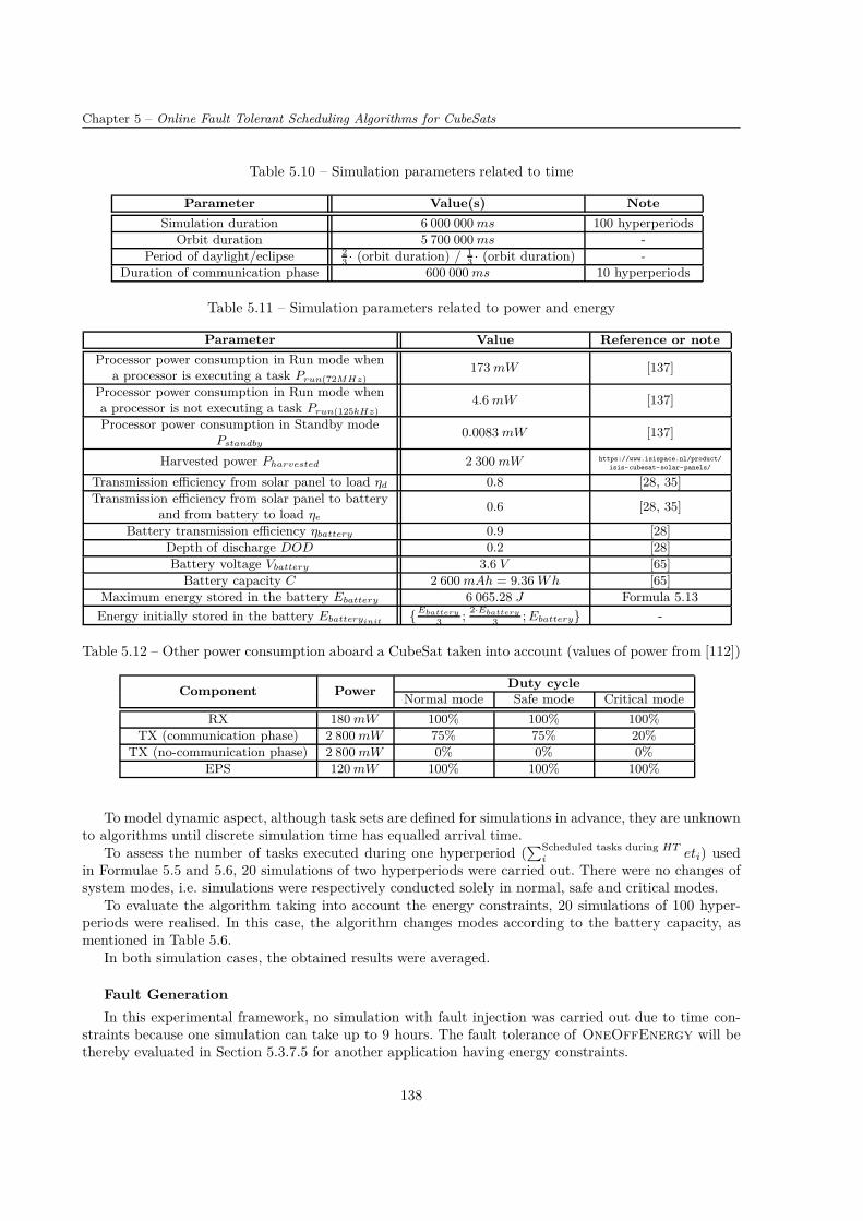
Chapter 5 – Online Fault Tolerant Scheduling Algorithms for CubeSats

Table 5.10 – Simulation parameters related to time

Parameter Value(s) Note

Simulation duration 6 000 000 ms 100 hyperperiods

Orbit duration 5 700 000 ms -

Period of daylight/eclipse 23· (orbit duration) / 1

3· (orbit duration) -

Duration of communication phase 600 000 ms 10 hyperperiods

Table 5.11 – Simulation parameters related to power and energy

Parameter Value Reference or note

Processor power consumption in Run mode whena processor is executing a task Prun(72MHz)

173 mW [137]

Processor power consumption in Run mode whena processor is not executing a task Prun(125kHz)

4.6 mW [137]

Processor power consumption in Standby modePstandby

0.0083 mW [137]

Harvested power Pharvested 2 300 mW https://www.isispace.nl/product/

isis-cubesat-solar-panels/

Transmission efficiency from solar panel to load ηd 0.8 [28, 35]

Transmission efficiency from solar panel to batteryand from battery to load ηe

0.6 [28, 35]

Battery transmission efficiency ηbattery 0.9 [28]

Depth of discharge DOD 0.2 [28]

Battery voltage Vbattery 3.6 V [65]

Battery capacity C 2 600 mAh = 9.36 W h [65]

Maximum energy stored in the battery Ebattery 6 065.28 J Formula 5.13

Energy initially stored in the battery Ebatteryinit Ebattery

3;

2·Ebattery

3; Ebattery -

Table 5.12 – Other power consumption aboard a CubeSat taken into account (values of power from [112])

Component PowerDuty cycle

Normal mode Safe mode Critical mode

RX 180 mW 100% 100% 100%

TX (communication phase) 2 800 mW 75% 75% 20%

TX (no-communication phase) 2 800 mW 0% 0% 0%

EPS 120 mW 100% 100% 100%

To model dynamic aspect, although task sets are defined for simulations in advance, they are unknownto algorithms until discrete simulation time has equalled arrival time.

To assess the number of tasks executed during one hyperperiod (∑Scheduled tasks during HT

i eti) usedin Formulae 5.5 and 5.6, 20 simulations of two hyperperiods were carried out. There were no changes ofsystem modes, i.e. simulations were respectively conducted solely in normal, safe and critical modes.

To evaluate the algorithm taking into account the energy constraints, 20 simulations of 100 hyper-periods were realised. In this case, the algorithm changes modes according to the battery capacity, asmentioned in Table 5.6.

In both simulation cases, the obtained results were averaged.

Fault Generation

In this experimental framework, no simulation with fault injection was carried out due to time con-straints because one simulation can take up to 9 hours. The fault tolerance of OneOffEnergy will bethereby evaluated in Section 5.3.7.5 for another application having energy constraints.

138

5.3. Energy-Aware Algorithm

5.3.4.2 Metrics

To analyse the algorithm performances, we put into practice, similarly to the previous evaluations, therejection rate, which is the ratio of rejected tasks to all arriving tasks, and the system load standing forthe number of processors executing a task at a given time instant. The processor load is then computed asthe system load divided by the number of processors. Since our system model considers that a processorcan be in Run or Standby mode, we distinguish two processor loads: the one where all system processorsare considered and the one where only processors in Run mode are taken into account. This differentiationallows us to better assess the utilisation of processors.

5.3.5 Results for CubeSats

In this section, we first calculate the energy balance on board of a CubeSat and then we assess theperformances of OneOffEnergy.

5.3.5.1 Energy Balance

First of all, we compute the theoretical processor load for each mode (normal, safe and critical) whenconsidering both maximum and mean execution times of each task based on Table 5.9. The results aredepicted in Figures 5.24 representing such a processor load respectively for both communication phasesas a function of the number of processors. Since several processors are switched in safe and critical modes,whose number is in Table 5.8, we compute the theoretical processor load from two points of view. On theone hand, we consider all system processors regardless of their operating mode and plot the results bysolid lines. On the other hand, we take into account only processors operating in Run mode and representthe corresponding results by dashed lines.

Figures 5.24 shows that the theoretical processor load depends on the mode and consequently onthe number of tasks. In fact, the modes are chosen according to the battery capacity and each modeauthorises only tasks having a given priority level or higher. It can be seen that, when considering onlyprocessors in Run mode, the theoretical processor load is sometimes constant (for example between 5 and6 processors), which is due to the same task input regardless of the number of system processors and thefloor function when switching processors to Standby mode.

Figures 5.25 depict the rejection rate for three modes (normal, safe and critical) as a function of thenumber of processors. In this figure and in this figure only, the rejection rate is computed consideringonly the authorised tasks, i.e. although low-priority tasks are not executed in a given mode, they donot exceptionally contribute to this metric in order to evaluate the ability to schedule the authorisedtasks. Normal mode has the highest rejection rate because the system deals with all tasks no mattertheir priority. In safe and critical modes, only task with higher priority are authorised to be executed.Consequently, there are less tasks to be scheduled and lower or none rejection rate.

Next, based on the data of the executed tasks, we compute the energy consumption using Formulae 5.5and 5.6. To represent the worst-case scenario, we consider that all processors are always in Run modeand none of them is put into Standby mode. Figures 5.26 show the useful and idle energy consumptionof CubeSat processors in three system modes during two hyperperiods as a function of the number ofprocessors during the communication phase. It is observed that once processors can accommodate alltasks, the useful energy consumption remains the same and the higher the number of processors, thehigher the idle energy consumption. The energy consumption due to idle processors is negligible whencompared to the one when processors are executing.

The simulations during the no-communication phase were also carried out. The results are qualitativelysimilar to the ones obtained during the communication phase and the values are slightly lower.

Once the energy consumption of processors is evaluated, we determine the corresponding power ofprocessors using Formula 5.8. Taking into account also all CubeSat components, mentioned in Table 5.12,

139

Chapter 5 – Online Fault Tolerant Scheduling Algorithms for CubeSats

3 4 5 6 7 8 9 10Number of processors

0.2

0.4

0.6

0.8

1.0

1.2Th

eoretic

al proce

ssor lo

ad fo

r mea

n ex

ecution tim

e

(a) Mean et; Communication phase

3 4 5 6 7 8 9 10Number of processors

0.2

0.4

0.6

0.8

1.0

Theo

retic

al proce

ssor lo

ad fo

r mea

n ex

ecution tim

e

(b) Mean et; No-communication phase

3 4 5 6 7 8 9 10Number of processors

0.25

0.50

0.75

1.00

1.25

1.50

1.75

2.00

Theo

retic

al proce

ssor lo

ad fo

r max

imum

exe

cutio

n tim

e

(c) Maximum et; Communication phase

3 4 5 6 7 8 9 10Number of processors

0.25

0.50

0.75

1.00

1.25

1.50

1.75

Theo

retic

al proce

ssor lo

ad fo

r max

imum

exe

cutio

n tim

e

(d) Maximum et; No-communicationphase

Figure 5.24 – Theoretical processor load when considering maximum and mean execution times (et) ofeach task

3 4 5 6 7 8 9 10Number of processors

0.000

0.005

0.010

0.015

0.020

0.025

0.030

0.035 Normal modeSafe modeCritical mode

(a) Communication phase

3 4 5 6 7 8 9 10Number of processors

0.000

0.025

0.050

0.075

0.100

0.125

0.150Normal modeSafe modeCritical mode

(b) No-communication phase

Figure 5.25 – Rejection rate for three system modes as a function of the number of processors

Formula 5.9 gives the overall CubeSat power consumption. The results are depicted in Figures 5.27representing the power in three system modes as a function of the number of processors.

We notice that the power is significantly higher during the communication phase than during the no-communication phase. This difference is due to the radio communication transmitter consuming 2.8 Wand its duty cycle of 75% in normal and safe modes during the communication phase. Moreover, thepower required in safe and critical modes is lower than the one in normal mode.

140

5.3. Energy-Aware Algorithm

3 4 5 6 7 8 9 10Number of processors

0.000

0.005

0.010

0.015

0.020

Ener

gy c

onsu

mpt

ion

(Wh)

Useful energy consumptionIdle energy consumption

(a) Normal mode

3 4 5 6 7 8 9 10Number of processors

0.000

0.002

0.004

0.006

0.008

0.010

0.012

0.014

Ener

gy c

onsu

mpt

ion

(Wh)

Useful energy consumptionIdle energy consumption

(b) Safe mode

3 4 5 6 7 8 9 10Number of processors

0.000

0.001

0.002

0.003

0.004

0.005

0.006

0.007

Ener

gy c

onsu

mpt

ion

(Wh)

Useful energy consumptionIdle energy consumption

(c) Critical mode

Figure 5.26 – Useful and idle energy consumptions during two hyperperiods as a function of the numberof processors (communication phase)

3 4 5 6 7 8 9 10Number of processors

0.0

0.5

1.0

1.5

2.0

2.5

3.0

Powe

r (W

)

Normal modeSafe modeCritical mode

(a) Communication phase

3 4 5 6 7 8 9 10Number of processors

0.0

0.2

0.4

0.6

0.8

Powe

r (W

)

Normal modeSafe modeCritical mode

(b) No-communication phase

Figure 5.27 – CubeSat power consumption in three system modes as a function of the number of processors

Finally, we evaluate the energy balance aboard a CubeSat. Thus, we compare the energy suppliedby the solar panel during the daylight to charge the battery Esupplied as expressed by Formula 5.11 andthe energy needed during the eclipse to power the CubeSat Eneeded, as given by Formula 5.12. Sincethe communication phase occurs at most once per CubeSat orbit and lasts only for 10 minutes, whichcorresponds to 10 hyperperiods, we examine two cases (as introduced in Section 5.3.4.1): (i) if there isno communication at all during a given period, the system functions in the no-communication phaseonly, and (ii) if a communication takes place during a given period, the system experiences both thecommunication phase and the no-communication phase. The former case is denoted by NCP, while thelatter one by CP+NCP. The results are plotted in Figures 5.28 respectively depicting two cases forEsupplied and Eneeded for a system composed of 3, 6 or 9 processors.

The higher the number of processors, the higher the power PCubeSat, the higher the energy neededin the eclipse Eneeded, the lower the power to recharge the battery Pcharge and therefore the lower thevalue of the energy Esupplied. It is worth noticing the battery capacity (Ebattery = 6.1 kJ) is sufficient toprovide enough energy for Eneeded < Ebattery regardless of system mode. On the one hand, while normalmode functions well during the no-communication phase because the energy supplied Esupplied coversall energy expenses Eneeded, normal mode experiences energy shortages during the communication phaseowing to EneededCP +NCP

> EsuppliedNCPall the time for any number of processors. On the other hand,

although the communication phase is very demanding, the energy supplied in critical mode Esupplied isalways sufficient to the demand in such a mode and there is never lack of energy even in the worst-casescenario (CP+NCP, P = 10).

We conclude that for CubeSats, whose payload does not require a lot of power, e.g. measurement ofelectron density, it is useless to develop a specific algorithm optimising the schedule taking into accountenergy harvesting and consumption. In fact, a simple check of the energy level available in the batteryand several operating system modes are sufficient.

141

Chapter 5 – Online Fault Tolerant Scheduling Algorithms for CubeSats

EsuppliedNCP EsuppliedCP+NCP EneededNCP EneededCP+NCP

Type of energy0

1000

2000

3000

4000

5000

Energy

(J)

Normal modeSafe modeCritical mode

(a) P = 3

EsuppliedNCP EsuppliedCP+NCP EneededNCP EneededCP+NCP

Type of energy0

1000

2000

3000

4000

5000

Energy

(J)

Normal modeSafe modeCritical mode

(b) P = 6

EsuppliedNCP EsuppliedCP+NCP EneededNCP EneededCP+NCP

Type of energy0

1000

2000

3000

4000

5000

Energy

(J)

Normal modeSafe modeCritical mode

(c) P = 10

Figure 5.28 – Comparison of the energy supplied by the solar panel during the daylight to charge thebattery and the energy needed during the eclipse to power the CubeSat

5.3.5.2 Algorithm Performances

The preceding section analysed results based on the evaluation of the energy balance in each systemmode. The aim of this section is to evaluate the performances of OneOffEnergy when operating onboard of a CubeSat.

We analyse two scenarios. The first one considers that the communication phase occurs during theeclipse, while the second one considers it during the daylight. In both cases, the initial battery capacityis set at one third of the maximum battery capacity. We conduct simulations for 100 hyperperiods, whichis more than one orbit duration.

Figures 5.29 and 5.31 plot the energy level in the battery against time. At the bottom of the figures,black and yellow colours respectively indicate the eclipse and the daylight. The vertical dashed lines marka change of mode.

Regardless of when the communication phase occurs, Figures 5.29 and 5.31 show that no energyshortage occurs and a CubeSat can operate in one of its modes. Furthermore, the battery is charged fromapproximately one sixth to its full capacity within less than one daylight, which confirms that the batterycan be sufficiently replenished.

Figures 5.30 and 5.32 represent the system and processor loads in the course of time. As definedin Section 5.3.4.2, the figures show the processor load when all system processors are considered (bluecurve) and the one taking into account processors in Run mode only (red curve). In order to enhance thereadability, the loads are computed within the window of size 10 s within one mode and averaged. Theeclipse and daylight periods and the mode changes are also plotted.

The system and processor loads remain almost constant in a given phase, which is due to the executionof the same tasks related to CubeSat housekeeping. We notice that when the communication phase occurs(at 900000ms if it takes place during the eclipse, or at 3000000ms otherwise) and lasts for 10 hyperperiods,i.e. 600000ms, the system and processor loads are higher to satisfy the demand and schedule tasks relatedto the communication.

As stated in Table 5.11, simulations (regardless of when the communication phase occurs) with theinitial battery capacity respectively equal to 2

3 · Ebattery and Ebattery were also carried out. Thanks tohigher initial battery capacity, the system spends more time in normal mode instead of safe one and itconsequently executes more tasks and its rejection rate is lower. Actually, due to energy savings, taskshaving the lowest priority are automatically rejected in safe mode, which increases the rejection rate.

The dependency of the rejection rate on the number of processors and the initial energy level in the bat-tery when the communication phase occurs respectively in the eclipse and in the daylight are respectivelydepicted in Figures 5.33. It can be observed that if the communication phase takes place during the eclipse,the rejection rate is higher (up to almost 50% for a 3-processor system with Ebatteryinit

= 13 · Ebattery)

than if it occurs during the daylight (17% for a 3-processor system with Ebatteryinit= 1

3 · Ebattery) dueto higher energy consumption.

142

5.3. Energy-Aware Algorithm

0 1000 2000 3000 4000 5000 6000Time (s)

0

1000

2000

3000

4000

5000

6000

Energy

in battery (J)

Mode S N

(a) P = 3

0 1000 2000 3000 4000 5000 6000Time (s)

0

1000

2000

3000

4000

5000

6000

Energy

in battery (J)

Mode S N

(b) P = 6

0 1000 2000 3000 4000 5000 6000Time (s)

0

1000

2000

3000

4000

5000

6000

Energy

in battery (J)

Mode S N

(c) P = 9

Figure 5.29 – Energy in the battery against time (communication phase in the eclipse; Ebatteryinit=

13 · Ebattery) 8

0 1000 2000 3000 4000 5000 6000Time (s)

0

1

2

3

System

load

Mode S NMode S N

0.5

0.6

0.7

0.8

0.9

Proc

essor loa

d

(a) P = 3

0 1000 2000 3000 4000 5000 6000Time (s)

0

1

2

3

4

5

6

System

load

Mode S NMode S N

0.25

0.30

0.35

0.40

0.45

0.50

0.55

0.60

Proc

esso

r loa

d(b) P = 6

0 1000 2000 3000 4000 5000 6000Time (s)

0123456789

System

load

Mode S NMode S N

0.15

0.20

0.25

0.30

0.35

0.40

Proc

essor loa

d

(c) P = 9

Figure 5.30 – System and processor loads against time (communication phase in the eclipse; Ebatteryinit=

13 · Ebattery)

0 1000 2000 3000 4000 5000 6000Time (s)

0

1000

2000

3000

4000

5000

6000

Energy

in battery (J)

Mode S N

(a) P = 3

0 1000 2000 3000 4000 5000 6000Time (s)

0

1000

2000

3000

4000

5000

6000

Energy

in battery (J)

Mode S N

(b) P = 6

0 1000 2000 3000 4000 5000 6000Time (s)

0

1000

2000

3000

4000

5000

6000

Energy

in battery (J)

Mode S N

(c) P = 9

Figure 5.31 – Energy in the battery against time (communication in the daylight; Ebatteryinit= 1

3 ·Ebattery)

In compliance with the results from the preceding section, we conclude that CubeSats containing onlylow power consumption payload do not take a risk to experience any energy shortage because the suppliedenergy covers all energy expenses. Their energy balance is overestimated in order not to jeopardise themission because of an energy issue.

To further analyse the performances of the proposed algorithm, we study another experiment scenario.Our aim is to compare OneOffEnergy with other simpler algorithms and evaluate its efficiency andfault tolerance.

8. S and N denote safe mode and normal mode, respectively.

143

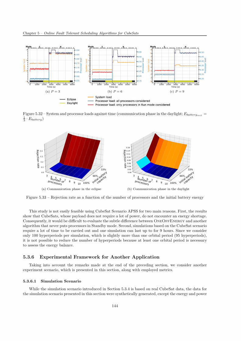
Chapter 5 – Online Fault Tolerant Scheduling Algorithms for CubeSats

0 1000 2000 3000 4000 5000 6000Time (s)

0

1

2

3

System

load

Mode S NMode S N

0.55

0.60

0.65

0.70

0.75

0.80

0.85

0.90

Proc

essor loa

d

(a) P = 3

0 1000 2000 3000 4000 5000 6000Time (s)

0

1

2

3

4

5

6

System

load

Mode S NMode S N

0.35

0.40

0.45

0.50

0.55

0.60

0.65

Proc

esso

r loa

d

(b) P = 6

0 1000 2000 3000 4000 5000 6000Time (s)

0123456789

System

load

Mode S NMode S N

0.20

0.25

0.30

0.35

0.40

0.45

0.50

Proc

essor loa

d

(c) P = 9

Figure 5.32 – System and processor loads against time (communication phase in the daylight; Ebatteryinit=

13 · Ebattery)

Initi

al battery

capa

city

33%

66%

100%Number of

processors

3 4 5 6 7 8 9 10

Rejection rate

0.0

0.1

0.2

0.3

0.4

(a) Communication phase in the eclipse

Initi

al battery

capa

city

33%

66%

100%Number of

processors

3 4 5 6 7 8 9 10

Rejection rate

0.000.020.040.060.080.100.120.140.16

(b) Communication phase in the daylight

Figure 5.33 – Rejection rate as a function of the number of processors and the initial battery energy

This study is not easily feasible using CubeSat Scenario APSS for two main reasons. First, the resultsshow that CubeSats, whose payload does not require a lot of power, do not encounter an energy shortage.Consequently, it would be difficult to evaluate the subtle difference between OneOffEnergy and anotheralgorithm that never puts processors in Standby mode. Second, simulations based on the CubeSat scenariorequire a lot of time to be carried out and one simulation can last up to for 9 hours. Since we consideronly 100 hyperperiods per simulation, which is slightly more than one orbital period (95 hyperperiods),it is not possible to reduce the number of hyperperiods because at least one orbital period is necessaryto assess the energy balance.

5.3.6 Experimental Framework for Another Application

Taking into account the remarks made at the end of the preceding section, we consider anotherexperiment scenario, which is presented in this section, along with employed metrics.

5.3.6.1 Simulation Scenario

While the simulation scenario introduced in Section 5.3.4 is based on real CubeSat data, the data forthe simulation scenario presented in this section were synthetically generated, except the energy and power

144

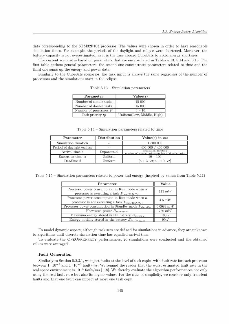
5.3. Energy-Aware Algorithm

data corresponding to the STM32F103 processor. The values were chosen in order to have reasonablesimulation times. For example, the periods of the daylight and eclipse were shortened. Moreover, thebattery capacity is not overestimated, as it is the case aboard CubeSats to avoid energy shortages.

The current scenario is based on parameters that are encapsulated in Tables 5.13, 5.14 and 5.15. Thefirst table gathers general parameters, the second one concentrates parameters related to time and thethird one sums up the energy and power data.

Similarly to the CubeSats scenarios, the task input is always the same regardless of the number ofprocessors and the simulations start in the eclipse.

Table 5.13 – Simulation parameters

Parameter Value(s)

Number of simple tasks 15 000

Number of double tasks 15 000

Number of processors P 3 – 10

Task priority tp Uniform(Low, Middle, High)

Table 5.14 – Simulation parameters related to time

Parameter Distribution Value(s) in ms

Simulation duration - 1 500 000

Period of daylight/eclipse - 400 000 / 400 000

Arrival time a Exponential simulation durationnumber of simple tasks+number of double tasks

Execution time et Uniform 10 – 100

Deadline d Uniform Ja + 3 · et; a + 10 · etK

Table 5.15 – Simulation parameters related to power and energy (inspired by values from Table 5.11)

Parameter Value

Processor power consumption in Run mode when aprocessor is executing a task Prun(72MHz)

173 mW

Processor power consumption in Run mode when aprocessor is not executing a task Prun(125kHz)

4.6 mW

Processor power consumption in Standby mode Pstandby 0.0083 mW

Harvested power Pharvested 750 mW

Maximum energy stored in the battery Ebattery 100 J

Energy initially stored in the battery Ebatteryinit 90 J

To model dynamic aspect, although task sets are defined for simulations in advance, they are unknownto algorithms until discrete simulation time has equalled arrival time.

To evaluate the OneOffEnergy performances, 20 simulations were conducted and the obtainedvalues were averaged.

Fault Generation

Similarly to Section 5.2.3.1, we inject faults at the level of task copies with fault rate for each processorbetween 1 · 10−5 and 1 · 10−3 fault/ms. We remind the reader that the worst estimated fault rate in thereal space environment is 10−5 fault/ms [118]. We thereby evaluate the algorithm performances not onlyusing the real fault rate but also its higher values. For the sake of simplicity, we consider only transientfaults and that one fault can impact at most one task copy.

145

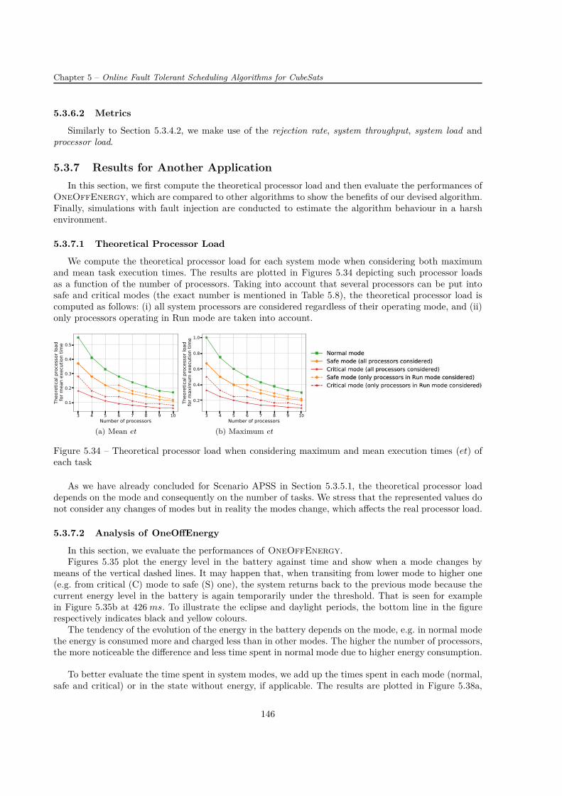
Chapter 5 – Online Fault Tolerant Scheduling Algorithms for CubeSats

5.3.6.2 Metrics

Similarly to Section 5.3.4.2, we make use of the rejection rate, system throughput, system load andprocessor load.

5.3.7 Results for Another Application

In this section, we first compute the theoretical processor load and then evaluate the performances ofOneOffEnergy, which are compared to other algorithms to show the benefits of our devised algorithm.Finally, simulations with fault injection are conducted to estimate the algorithm behaviour in a harshenvironment.

5.3.7.1 Theoretical Processor Load

We compute the theoretical processor load for each system mode when considering both maximumand mean task execution times. The results are plotted in Figures 5.34 depicting such processor loadsas a function of the number of processors. Taking into account that several processors can be put intosafe and critical modes (the exact number is mentioned in Table 5.8), the theoretical processor load iscomputed as follows: (i) all system processors are considered regardless of their operating mode, and (ii)only processors operating in Run mode are taken into account.

3 4 5 6 7 8 9 10Number of processors

0.1

0.2

0.3

0.4

0.5

Theo

retic

al proce

ssor lo

ad fo

r mea

n ex

ecution tim

e

(a) Mean et

3 4 5 6 7 8 9 10Number of processors

0.2

0.4

0.6

0.8

1.0

Theo

retic

al proce

ssor lo

ad fo

r max

imum

exe

cutio

n tim

e

(b) Maximum et

Figure 5.34 – Theoretical processor load when considering maximum and mean execution times (et) ofeach task

As we have already concluded for Scenario APSS in Section 5.3.5.1, the theoretical processor loaddepends on the mode and consequently on the number of tasks. We stress that the represented values donot consider any changes of modes but in reality the modes change, which affects the real processor load.

5.3.7.2 Analysis of OneOffEnergy

In this section, we evaluate the performances of OneOffEnergy.Figures 5.35 plot the energy level in the battery against time and show when a mode changes by

means of the vertical dashed lines. It may happen that, when transiting from lower mode to higher one(e.g. from critical (C) mode to safe (S) one), the system returns back to the previous mode because thecurrent energy level in the battery is again temporarily under the threshold. That is seen for examplein Figure 5.35b at 426 ms. To illustrate the eclipse and daylight periods, the bottom line in the figurerespectively indicates black and yellow colours.

The tendency of the evolution of the energy in the battery depends on the mode, e.g. in normal modethe energy is consumed more and charged less than in other modes. The higher the number of processors,the more noticeable the difference and less time spent in normal mode due to higher energy consumption.

To better evaluate the time spent in system modes, we add up the times spent in each mode (normal,safe and critical) or in the state without energy, if applicable. The results are plotted in Figure 5.38a,

146

5.3. Energy-Aware Algorithm

0 250 500 750 1000 1250 1500Time (s)

0

20

40

60

80

100

Energy

in battery (J)

Mode N S C S N S C S N

(a) P = 3

0 250 500 750 1000 1250 1500Time (s)

0

20

40

60

80

100

Energy

in battery (J)

Mode N S C SCS N S C SCS N

(b) P = 6

0 250 500 750 1000 1250 1500Time (s)

0

20

40

60

80

100

Energy

in battery (J)

Mode N S C S N S C S N

(c) P = 9

Figure 5.35 – Energy in the battery against time 9

which represents such times within one simulation duration as a function of the number of processors.As we have already concluded previously, when the number of processors increases, the times spent innormal and then safe mode are shorter.

As a consequence of spending more time in normal mode instead of safe one or critical one, thesystem executes more tasks and its rejection rate is lower. Actually, due to energy savings in safe andcritical modes, low-priority tasks are automatically rejected in safe and critical modes, which increasesthe rejection rate. Figure 5.40a representing the rejection rate as a function of the number of processorsshows that the lower the number of processors, the lower the rejection rate because the system consumesless energy.

Figures 5.36 depict the system and processor loads in the course of time. As defined in Section 5.3.6.2,we distinguish the processor load when all system processors are considered (blue curve) and the onetaking into account processors in Run mode only (red curve). To enhance the readability, the loads arecomputed within the window of size 10s within one mode and averaged. The eclipse and daylight periodsare indicated by the black-and-yellow line. The mode changes are plotted by the vertical dashed lines.

In general, the higher the number of processors, the lower the processor load because the number oftasks to be executed is unchanged and the system load thereby remains the same. When several processorsare switched into Standby mode (during safe or critical mode), the load of processors being in Run modeis higher than the one considering all system processors. Moreover, the system and processor loads donot significantly vary within one mode because the number of tasks to be executed does not change.

0 250 500 750 1000 1250 1500Time (s)

0

1

2

3

System

load

Mode N S C S N S C S NMode N S C S N S C S N

0.2

0.3

0.4

0.5

0.6

0.7

Proc

essor loa

d

(a) P = 3

0 250 500 750 1000 1250 1500Time (s)

0

1

2

3

4

5

6

System

load

Mode N S C SCS N S C SCS NMode N S C SCS N S C SCS N

0.2

0.4

0.6

0.8

1.0

Proc

essor loa

d

(b) P = 6

0 250 500 750 1000 1250 1500Time (s)

0123456789

System

load

Mode N S C S N S C S NMode N S C S N S C S N

0.05

0.10

0.15

0.20

0.25Proc

essor loa

d

(c) P = 9

Figure 5.36 – System and processor loads against time

9. N, S and C denote normal, safe and critical modes, respectively.

147

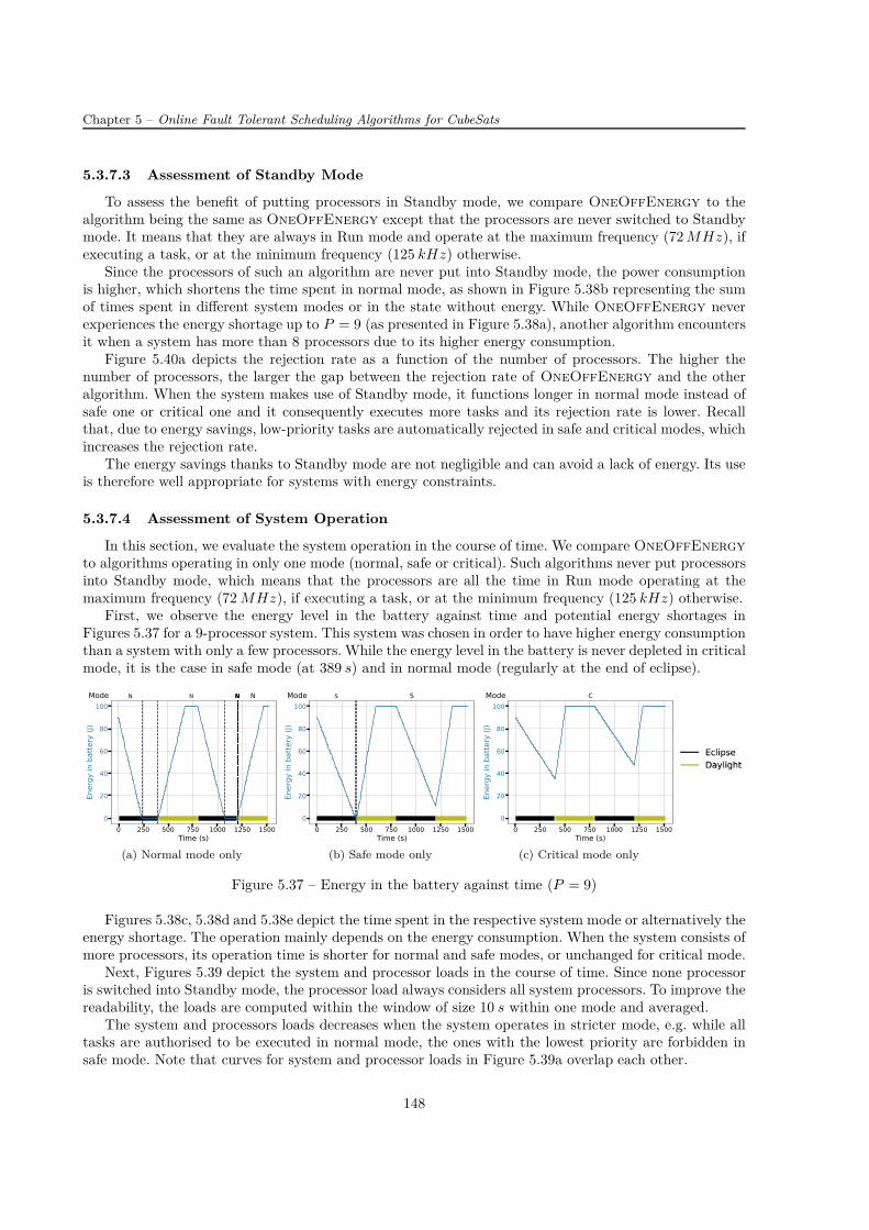
Chapter 5 – Online Fault Tolerant Scheduling Algorithms for CubeSats

5.3.7.3 Assessment of Standby Mode

To assess the benefit of putting processors in Standby mode, we compare OneOffEnergy to thealgorithm being the same as OneOffEnergy except that the processors are never switched to Standbymode. It means that they are always in Run mode and operate at the maximum frequency (72 MHz), ifexecuting a task, or at the minimum frequency (125 kHz) otherwise.

Since the processors of such an algorithm are never put into Standby mode, the power consumptionis higher, which shortens the time spent in normal mode, as shown in Figure 5.38b representing the sumof times spent in different system modes or in the state without energy. While OneOffEnergy neverexperiences the energy shortage up to P = 9 (as presented in Figure 5.38a), another algorithm encountersit when a system has more than 8 processors due to its higher energy consumption.

Figure 5.40a depicts the rejection rate as a function of the number of processors. The higher thenumber of processors, the larger the gap between the rejection rate of OneOffEnergy and the otheralgorithm. When the system makes use of Standby mode, it functions longer in normal mode instead ofsafe one or critical one and it consequently executes more tasks and its rejection rate is lower. Recallthat, due to energy savings, low-priority tasks are automatically rejected in safe and critical modes, whichincreases the rejection rate.

The energy savings thanks to Standby mode are not negligible and can avoid a lack of energy. Its useis therefore well appropriate for systems with energy constraints.

5.3.7.4 Assessment of System Operation

In this section, we evaluate the system operation in the course of time. We compare OneOffEnergyto algorithms operating in only one mode (normal, safe or critical). Such algorithms never put processorsinto Standby mode, which means that the processors are all the time in Run mode operating at themaximum frequency (72 MHz), if executing a task, or at the minimum frequency (125 kHz) otherwise.

First, we observe the energy level in the battery against time and potential energy shortages inFigures 5.37 for a 9-processor system. This system was chosen in order to have higher energy consumptionthan a system with only a few processors. While the energy level in the battery is never depleted in criticalmode, it is the case in safe mode (at 389 s) and in normal mode (regularly at the end of eclipse).

0 250 500 750 1000 1250 1500Time (s)

0

20

40

60

80

100

Energy

in battery (J)

Mode N N NNNN N

(a) Normal mode only

0 250 500 750 1000 1250 1500Time (s)

0

20

40

60

80

100

Energy

in battery (J)

Mode S S

(b) Safe mode only

0 250 500 750 1000 1250 1500Time (s)

0

20

40

60

80

100

Energy

in battery (J)

Mode C

(c) Critical mode only

Figure 5.37 – Energy in the battery against time (P = 9)

Figures 5.38c, 5.38d and 5.38e depict the time spent in the respective system mode or alternatively theenergy shortage. The operation mainly depends on the energy consumption. When the system consists ofmore processors, its operation time is shorter for normal and safe modes, or unchanged for critical mode.

Next, Figures 5.39 depict the system and processor loads in the course of time. Since none processoris switched into Standby mode, the processor load always considers all system processors. To improve thereadability, the loads are computed within the window of size 10 s within one mode and averaged.

The system and processors loads decreases when the system operates in stricter mode, e.g. while alltasks are authorised to be executed in normal mode, the ones with the lowest priority are forbidden insafe mode. Note that curves for system and processor loads in Figure 5.39a overlap each other.

148

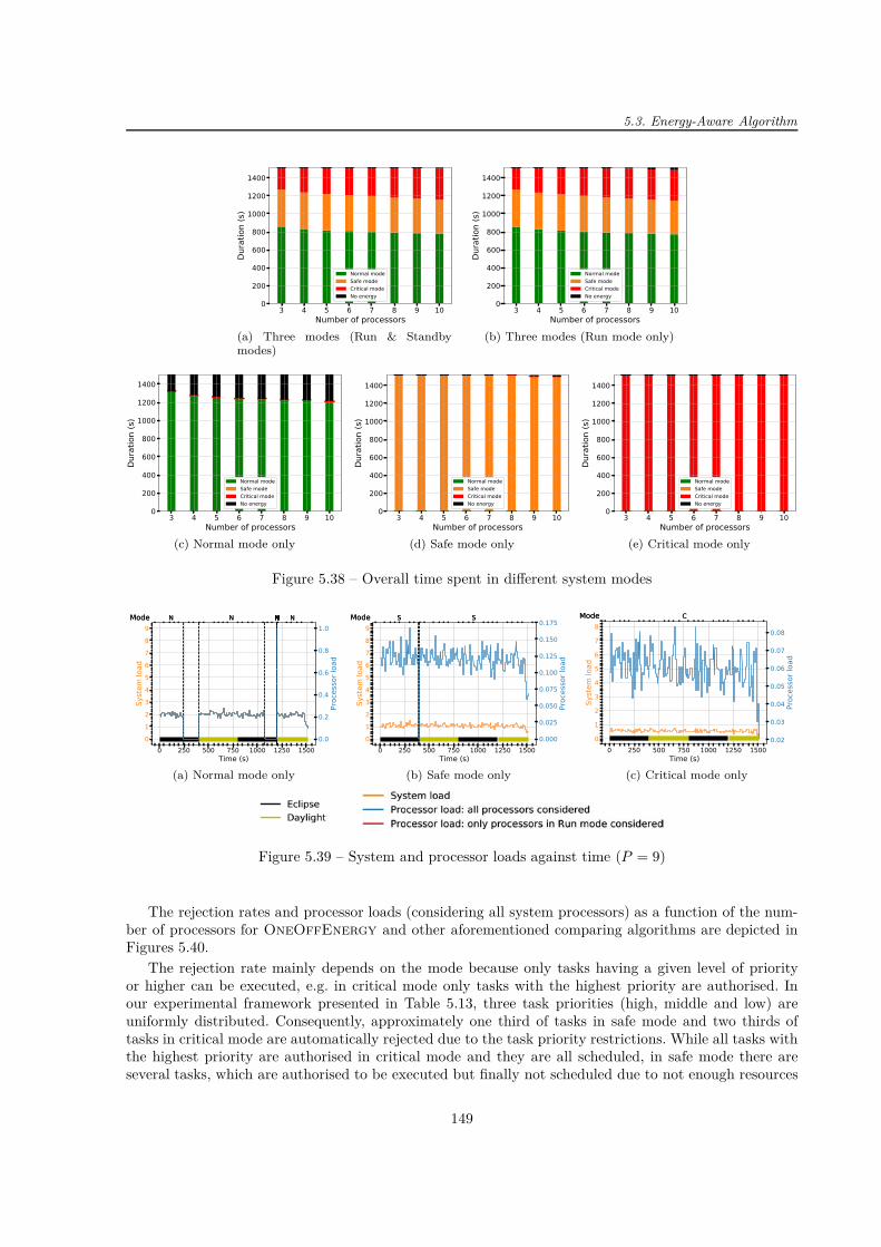
5.3. Energy-Aware Algorithm

3 4 5 6 7 8 9 10Number of processors

0

200

400

600

800

1000

1200

1400

Dura

tion

(s)

Normal modeSafe modeCritical modeNo energy

(a) Three modes (Run & Standbymodes)

3 4 5 6 7 8 9 10Number of processors

0

200

400

600

800

1000

1200

1400

Dura

tion

(s)

Normal modeSafe modeCritical modeNo energy

(b) Three modes (Run mode only)

3 4 5 6 7 8 9 10Number of processors

0

200

400

600

800

1000

1200

1400

Dura

tion

(s)

Normal modeSafe modeCritical modeNo energy

(c) Normal mode only

3 4 5 6 7 8 9 10Number of processors

0

200

400

600

800

1000

1200

1400

Dura

tion

(s)

Normal modeSafe modeCritical modeNo energy

(d) Safe mode only

3 4 5 6 7 8 9 10Number of processors

0

200

400

600

800

1000

1200

1400

Dura

tion

(s)

Normal modeSafe modeCritical modeNo energy

(e) Critical mode only

Figure 5.38 – Overall time spent in different system modes

0 250 500 750 1000 1250 1500Time (s)

0123456789

System

load

Mode N N NNNN NMode N N NNNN N

0.0

0.2

0.4

0.6

0.8

1.0

Proc

essor loa

d

(a) Normal mode only

0 250 500 750 1000 1250 1500Time (s)

0123456789

System

load

Mode S SMode S S

0.000

0.025

0.050

0.075

0.100

0.125

0.150

0.175

Proc

esso

r loa

d

(b) Safe mode only

0 250 500 750 1000 1250 1500Time (s)

0

1

2

3

4

5

6

7

8

System

load

Mode CMode C

0.02

0.03

0.04

0.05

0.06

0.07

0.08

Proc

essor loa

d(c) Critical mode only

Figure 5.39 – System and processor loads against time (P = 9)

The rejection rates and processor loads (considering all system processors) as a function of the num-ber of processors for OneOffEnergy and other aforementioned comparing algorithms are depicted inFigures 5.40.

The rejection rate mainly depends on the mode because only tasks having a given level of priorityor higher can be executed, e.g. in critical mode only tasks with the highest priority are authorised. Inour experimental framework presented in Table 5.13, three task priorities (high, middle and low) areuniformly distributed. Consequently, approximately one third of tasks in safe mode and two thirds oftasks in critical mode are automatically rejected due to the task priority restrictions. While all tasks withthe highest priority are authorised in critical mode and they are all scheduled, in safe mode there areseveral tasks, which are authorised to be executed but finally not scheduled due to not enough resources

149

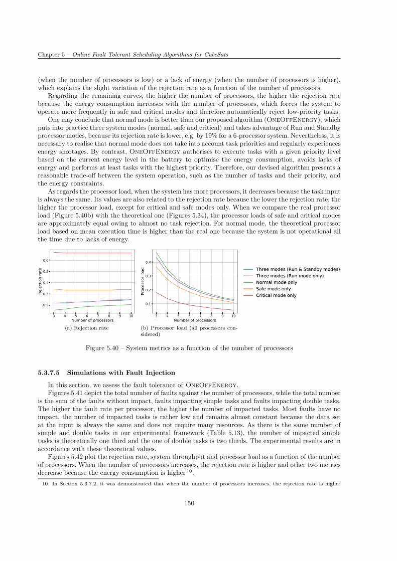
Chapter 5 – Online Fault Tolerant Scheduling Algorithms for CubeSats

(when the number of processors is low) or a lack of energy (when the number of processors is higher),which explains the slight variation of the rejection rate as a function of the number of processors.

Regarding the remaining curves, the higher the number of processors, the higher the rejection ratebecause the energy consumption increases with the number of processors, which forces the system tooperate more frequently in safe and critical modes and therefore automatically reject low-priority tasks.

One may conclude that normal mode is better than our proposed algorithm (OneOffEnergy), whichputs into practice three system modes (normal, safe and critical) and takes advantage of Run and Standbyprocessor modes, because its rejection rate is lower, e.g. by 19% for a 6-processor system. Nevertheless, it isnecessary to realise that normal mode does not take into account task priorities and regularly experiencesenergy shortages. By contrast, OneOffEnergy authorises to execute tasks with a given priority levelbased on the current energy level in the battery to optimise the energy consumption, avoids lacks ofenergy and performs at least tasks with the highest priority. Therefore, our devised algorithm presents areasonable trade-off between the system operation, such as the number of tasks and their priority, andthe energy constraints.

As regards the processor load, when the system has more processors, it decreases because the task inputis always the same. Its values are also related to the rejection rate because the lower the rejection rate, thehigher the processor load, except for critical and safe modes only. When we compare the real processorload (Figure 5.40b) with the theoretical one (Figures 5.34), the processor loads of safe and critical modesare approximately equal owing to almost no task rejection. For normal mode, the theoretical processorload based on mean execution time is higher than the real one because the system is not operational allthe time due to lacks of energy.

3 4 5 6 7 8 9 10Number of processors

0.2

0.3

0.4

0.5

0.6

Rejection rate

(a) Rejection rate

3 4 5 6 7 8 9 10Number of processors

0.1

0.2

0.3

0.4

Processor loa

d

(b) Processor load (all processors con-sidered)

Figure 5.40 – System metrics as a function of the number of processors

5.3.7.5 Simulations with Fault Injection

In this section, we assess the fault tolerance of OneOffEnergy.Figures 5.41 depict the total number of faults against the number of processors, while the total number

is the sum of the faults without impact, faults impacting simple tasks and faults impacting double tasks.The higher the fault rate per processor, the higher the number of impacted tasks. Most faults have noimpact, the number of impacted tasks is rather low and remains almost constant because the data setat the input is always the same and does not require many resources. As there is the same number ofsimple and double tasks in our experimental framework (Table 5.13), the number of impacted simpletasks is theoretically one third and the one of double tasks is two thirds. The experimental results are inaccordance with these theoretical values.

Figures 5.42 plot the rejection rate, system throughput and processor load as a function of the numberof processors. When the number of processors increases, the rejection rate is higher and other two metricsdecrease because the energy consumption is higher 10.

10. In Section 5.3.7.2, it was demonstrated that when the number of processors increases, the rejection rate is higher

150

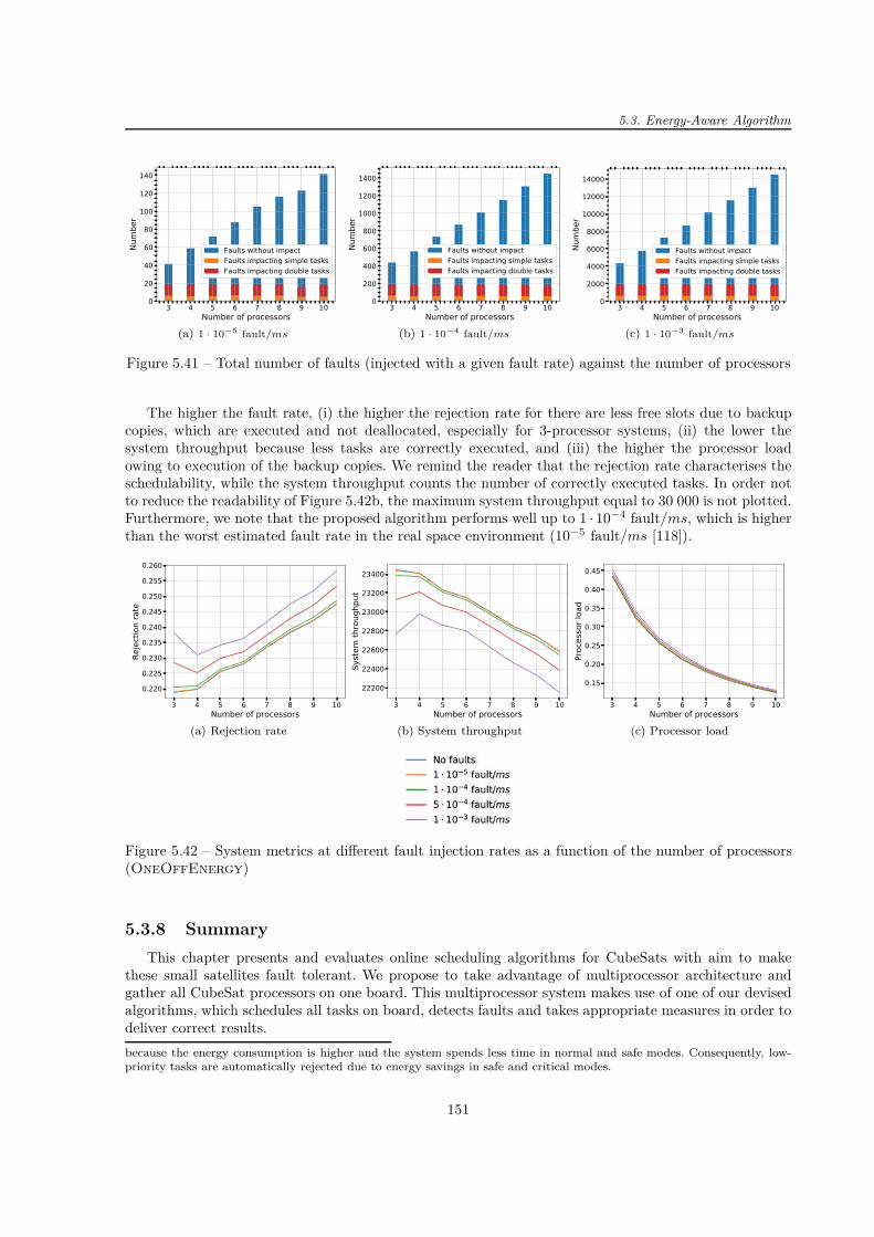
5.3. Energy-Aware Algorithm

3 4 5 6 7 8 9 10Number of processors

0

20

40

60

80

100

120

140

Number

Faults without impactFaults impacting simple tasksFaults impacting double tasks

(a) 1 · 10−5 fault/ms

3 4 5 6 7 8 9 10Number of processors

0

200

400

600

800

1000

1200

1400

Number

Faults without impactFaults impacting simple tasksFaults impacting double tasks

(b) 1 · 10−4 fault/ms

3 4 5 6 7 8 9 10Number of processors

0

2000

4000

6000

8000

10000

12000

14000

Number

Faults without impactFaults impacting simple tasksFaults impacting double tasks

(c) 1 · 10−3 fault/ms

Figure 5.41 – Total number of faults (injected with a given fault rate) against the number of processors

The higher the fault rate, (i) the higher the rejection rate for there are less free slots due to backupcopies, which are executed and not deallocated, especially for 3-processor systems, (ii) the lower thesystem throughput because less tasks are correctly executed, and (iii) the higher the processor loadowing to execution of the backup copies. We remind the reader that the rejection rate characterises theschedulability, while the system throughput counts the number of correctly executed tasks. In order notto reduce the readability of Figure 5.42b, the maximum system throughput equal to 30 000 is not plotted.Furthermore, we note that the proposed algorithm performs well up to 1 · 10−4 fault/ms, which is higherthan the worst estimated fault rate in the real space environment (10−5 fault/ms [118]).

3 4 5 6 7 8 9 10Number of processors

0.220

0.225

0.230

0.235

0.240

0.245

0.250

0.255

0.260

Rejection rate

(a) Rejection rate

3 4 5 6 7 8 9 10Number of processors

22200

22400

22600

22800

23000

23200

23400

System

throug

hput

(b) System throughput

3 4 5 6 7 8 9 10Number of processors

0.15

0.20

0.25

0.30

0.35

0.40

0.45Processor loa

d

(c) Processor load

Figure 5.42 – System metrics at different fault injection rates as a function of the number of processors(OneOffEnergy)

5.3.8 Summary

This chapter presents and evaluates online scheduling algorithms for CubeSats with aim to makethese small satellites fault tolerant. We propose to take advantage of multiprocessor architecture andgather all CubeSat processors on one board. This multiprocessor system makes use of one of our devisedalgorithms, which schedules all tasks on board, detects faults and takes appropriate measures in order todeliver correct results.

because the energy consumption is higher and the system spends less time in normal and safe modes. Consequently, low-priority tasks are automatically rejected due to energy savings in safe and critical modes.

151

Chapter 5 – Online Fault Tolerant Scheduling Algorithms for CubeSats

The first algorithm called OneOff considers all tasks as aperiodic tasks, the second one, namedOneOff&Cyclic, distinguishes aperiodic and periodic tasks when searching for a new schedule. Whereasthese two algorithms do not take energy constraints into account, the last proposed algorithm calledOneOffEnergy is energy-aware. All algorithms can use different ordering policies to sort a task queue.

The performances of OneOff and OneOff&Cyclic were studied for three different scenarios basedon two real CubeSat scenarios. It was shown that they are influenced by the system load and proportions ofsimple and double tasks to all tasks to be executed. Overall, the "Earliest Deadline" and "Earliest ArrivalTime" ordering policies perform well (measured by means of the rejection rate) for OneOff and the"Minimum Slack" ordering policy for OneOff&Cyclic. Furthermore, evaluating several ordering policiesat every scheduling search (method called "All techniques") does not perform better than aforementionedpolicies and its main drawback is longer algorithm run-time induced by multiple scheduling searchesbefore choosing the one minimising the rejection rate. Moreover, it is useless to consider systems withmore than six processors because there is already no rejection rate for well chosen ordering policies andit is better not to oversize the system.

Although the number of scheduling attempts is significantly lower for OneOff&Cyclic than forOneOff, the former algorithm carries out a search for a new schedule more quickly than the latter one.The scheduling time is shorter during the no-communication phase than during the communication phasefor there are less tasks to be scheduled. The method to reduce the number of scheduling searches cutsdown this number but at the cost of higher rejection rate, which is not compatible with our objectivefunction, to minimise the rejection rate, and the method is not used any longer.

The results demonstrate that OneOff&Cyclic does not generally perform as well as OneOff (interms of the rejection rate and scheduling time) in the context of CubeSats but it can be put into practicein other applications with much more benefit (for example in embedded systems with real-time and energyconstraints), where there are less scheduling triggers (less faults or less aperiodic tasks or less changes inset of periodic tasks) than in the studied application.

Therefore, we suggest that teams, which design their CubeSats gathering all processors on one board,should make use of OneOff when choosing a no-energy-aware algorithm.

The second part of this chapter is dedicated to an energy-aware version of OneOff. This modifiedalgorithm called OneOffEnergy takes advantage of two processor operating modes (Run and Standby)and it considers three system modes (normal, safe and critical) depending on the energy available inthe battery. The new enhanced algorithm was not only assessed for CubeSats but also in the context ofanother application having energy constraints.

The energy balance for CubeSat Scenario APSS showed that the communication phase requires a lotof energy mainly due to high power consumption of the transmitter (2.8W ). Although the communicationphase lasts for 10 minutes, which is rather short duration compared to the orbital period of 95 minutesand it occurs approximately six times out of fifteen daily orbits around the Earth, it may cause a lackof energy. Nevertheless, when OneOffEnergy is put into practice and a CubeSat operates within oneof the following modes: normal, safe and critical, the energy shortage does not take place. In fact, theenergy supplied is always sufficient to the demand in critical mode for values computed even in theworst-case scenario, i.e. when the communication phase occurs during the no-communication phase for a10-processor system.

We state that CubeSats, whose payload does not require a lot of power, e.g. measurement of electrondensity, do not experience any energy shortage. Consequently, they can use a simple algorithm, such asOneOffEnergy, to check the energy level in the battery capacity and choose one of the system modes(normal, safe or critical) according to the current available energy level.

Since the CubeSat scenario does not allow us to assess all performances of our proposed energy-awarealgorithm, we carry out simulations also for another energy-constrained application and compare theperformances of OneOffEnergy with other simpler algorithms. The main differences are as follows: (i)the data for the application were synthetically generated (instead of real data for CubeSats), (ii) the time

152

5.3. Energy-Aware Algorithm

spent in the daylight and eclipse were shortened to reduce the duration of the simulation, and (iii) thebattery capacity is not overestimated, as it is the case aboard CubeSats to avoid energy shortages.

We found out that putting the processors in Standby mode brings energy savings. These savingsallow the system to operate longer in normal or safe modes and consequently avoid automatic rejectionof low-priority tasks. Although a system operating in normal mode only has lower rejection rate thanthe one using OneOffEnergy (for example by 19% for the 6-processor system), it is not able to runall the time due to limited energy resources. In contrast, OneOffEnergy chooses one of the systemmodes (normal, safe or critical) according to the available energy stored in the battery, executes taskswith appropriate priorities to optimise the energy consumption and avoids lacks of energy. Therefore, ouralgorithm presents a reasonable trade-off between the system operation, such as the number of tasks andtheir priority, and the energy constraints.

Finally, it was found that all three presented algorithms (OneOff, OneOff&Cyclic and OneOff-Energy) perform well also in a harsh environment.

The achievements of this chapter were published in Proceedings of the 11th Workshop on ParallelProgramming and Run-Time Management Techniques for Many-Core Architectures / 9th Workshop onDesign Tools and Architectures for Multicore Embedded Computing Platforms (PARMA-DITAM) andof the Euromicro Conference on Digital System Design (DSD), both held in 2020.

153

Chapter 6

CONCLUSIONS

The thesis is aimed at providing multiprocessor systems with fault tolerance and is in particularconcerned with online mapping and scheduling of tasks on such systems in order to improve the systemreliability subject to various constraints regarding e.g. time, space, and energy. The applications of ourachievements are two-fold: (i) the primary/backup approach technique, which is a fault tolerant onebased on two task copies (primary and backup ones), and (ii) the CubeSat project, within framework ofwhich small satellites operate in the harsh space environment. In both cases, the system performancesare mainly evaluated by means of the rejection rate, the algorithm complexity measured by the numberof comparisons of evaluated slots or the scheduling time, and the resilience assessed by injecting faults.

Primary/Backup Approach Technique

Our achievements for the primary/backup (PB) approach (presented and discussed in Chapter 3)include the introduction of a new processor allocation policy (called the first found solution search: slotby slot), and of three new enhancing techniques (the restricted scheduling windows, limitation on thenumber of comparisons and several scheduling attempts). We also present a mathematical programmingformulation of the scheduling problem and carry out more general experiments to evaluate the faulttolerance of this approach.

The next five paragraphs enumerate the main results of the scheduling of the independent tasks. Thefirst four paragraphs predominantly cover our achievements for the analysis of the main already existingmethods for the PB approach. To the best of author’s knowledge, although these methods are often putinto practice, they have never been thoroughly analysed and compared. Our proposed enhancements forthe PB approach are described in the fifth paragraph.

Firstly, the results of the PB approach in itself (considered as the baseline) and the one with backupcopy (BC) overloading reveal that the BC overloading facilitates the reduction of the rejection rate (forexample by 14% for a 14-processor system). When the BC deallocation is then put into practice, theimprovement is even more noteworthy. For instance, for the 14-processor system, the gain is about 75%compared to the baseline PB approach and regardless of whether the BC overloading is implemented ornot. Moreover, it is shown that the BC overloading and the BC deallocation well cooperate.

Secondly, we analysed the active PB approach, i.e. a technique allowing the primary and backupcopies of the same task to be executed at the same time on different processors, which is not normallyauthorised. It is demonstrated that it is beneficial for systems dealing with tasks with tight deadline. Itreduces the rejection rate compared to the baseline. For the 14-processor system, there is a drop in therejection rate by about 17% for both the PB approach with BC deallocation and with or without BCoverloading.

Thirdly, three different processor allocation policies were analysed. Although the exhaustive search(ES) exhibits lower rejection rate than both the first found solution search - processor by processor (FFSSPbP) and the first found solution search - slot by slot (FFSS SbS), its number of comparisons related tothe algorithm run-time is significantly higher. The FFSS SbS performs better by all studied metrics thanthe FFSS PbP and it is 2-competitive in comparison to the optimal solution.

Fourthly, two scheduling search techniques were compared: the free slot search technique (FSST) andthe boundary schedule search technique (BSST). The BBST + ES exhibits similar rejection rate as theFSST + ES while the number of comparisons of the BSST is significantly higher than the one of the

155

Chapter 6 – Conclusions

FSST (more than twice as large). Therefore, the BSST is not a convenient scheduling search techniqueto reduce the algorithm run-time.

And fifthly, three techniques (the limitation on the number of comparisons, restricted scheduling win-dows and several scheduling attempts) and their combinations are analysed in terms of their performances.The results show that the best methods, which reduce both the rejection rate and the number of com-parisons, are (i) the limitation on the number of comparisons combined with two scheduling attempts at33% of the task window, and (ii) the limitation on the number of comparisons. The algorithm run-timeof the former technique is reduced by 23% (mean value) and 67% (maximum value) and its rejection rateis decreased by 4% compared to the primary/backup approach without any enhancing method.

To extend the analysis of the PB approach of the independent tasks to the dependent ones, we adaptedthe previously studied scheduling algorithm. When the search for a slot to schedule a task copy is carriedout by the BSST, the number of comparisons is significantly higher than the one based on the FSST.While the BSST scours all processors and tests all possible slots, the FSST conducts a search until asolution is found or all processors are tested. Consequently, the BSST + ES BC maxOverload, i.e. themethod based on the BSST and maximising the BC overloading, exhibits better performances than otherstudied techniques in terms of the rejection rate and system throughout but at the cost of the longeralgorithm run-time, except for the systems with only several processors. Furthermore, the FFSS SbS andFFSS PbP achieve similar performances but the FFSS SbS requires more comparisons.

Last but not least, simulations conducted for all presented algorithms unveil that the faults, havingfault rates even higher than the worst estimated fault rate in a harsh environment (1 · 10−5 fault/ms[118]), have a minimal impact on the scheduling algorithm. Regarding the dependent tasks, the spaceand time constraints due to task dependencies impose more restrictions on scheduling than faults.

Although a considerable amount of work was carried out for the PB approach, it was mainly concernedwith the system reliability. Therefore, we suggest as a possibility to follow up with the research taking intoaccount also energy aspect, for power consumption is one of the most important issues in multiprocessorembedded systems. Another possibility is to consider that the real computation time may be shorter thanthe worst-case computation time.

In addition, our results for dependent tasks show that there is a room for further improvement.Nevertheless, to yield better results, it will be necessary to focus on particular applications instead ofdevising general methods as we did.

CubeSats

To make CubeSats fault tolerant, in Chapter 5, we propose to take advantage of multiprocessorarchitecture and gather all CubeSat processors on one board 1. Such a multiprocessor system can make useof one of our devised algorithms, which schedules all tasks on board, detects faults and takes appropriatemeasures in order to deliver correct results.

The first algorithm called OneOff considers all tasks as aperiodic tasks, the second one, namedOneOff&Cyclic, distinguishes aperiodic and periodic tasks when searching for a new schedule. Whilethe first two presented algorithms do not take energy constraints into account, the last proposed algorithmcalled OneOffEnergy is energy-aware. All algorithms can use different ordering policies to sort a taskqueue. Overall, the "Earliest Deadline" ordering policy performs well in terms of the rejection rate andscheduling time for OneOff and the "Minimum Slack" ordering policy for OneOff&Cyclic.

All in all, the presented results based on two real CubeSat scenarios show that it is useless (from theviewpoint of the rejection rate) to consider systems with more than six processors and that OneOff

1. At present, every CubeSat system has in general one dedicated processor.

156

performs better than OneOff&Cyclic in terms of both the rejection rate and the scheduling time.OneOff&Cyclic can be more efficient in applications where there are only a few changes in the set ofperiodic tasks. We therefore recommend that teams designing CubeSats gathering all processors on oneboard should make use of OneOff when choosing a no-energy-aware algorithm. Nevertheless, it wouldbe better to apply an energy-aware algorithm, such as OneOffEnergy.

OneOffEnergy is a modified version of OneOff operating in two processor modes (Run andStandby) to save energy and it considers three system modes (normal, safe and critical) depending onthe current energy stored in the battery. OneOffEnergy was not only evaluated for CubeSats but alsoin the context of another energy-constrained application.

The energy balance for CubeSat Scenario APSS showed that the communication phase requires a hugeamount of energy mainly due to high power consumption of the transmitter. Compared to the CubeSatorbit duration taking 95 minutes, the communication phase lasts for 10 minutes but it may cause a lackof energy in the case if an energy-aware algorithm is not considered. If OneOffEnergy is implementedand a CubeSat operates within one of the system modes (normal, safe or critical), it does not take a riskto experience any energy shortage because the supplied energy covers all energy expenses.

Since the CubeSat scenario does not allow us to assess all performances of OneOffEnergy, wecarried out simulations also for another energy-constrained application and compare the performancesof OneOffEnergy with other simpler algorithms. The main differences are as follows: (i) the data forthe application were synthetically generated (instead of real data for CubeSats), (ii) the time spent inthe daylight and eclipse were shortened to reduce the duration of the simulation, and (iii) the batterycapacity is not overestimated, as it is the case aboard CubeSats to avoid energy shortages.

The energy savings obtained when putting processors in Standby mode are not negligible and can avoida lack of energy. Its use is thereby appropriate for systems with energy constraints because the systemoperates longer in normal or safe system modes and therefore avoid automatic rejection of low-prioritytasks.

A system operating in normal mode only exhibits lower rejection rate than the one using OneOff-Energy but it is not able to run all the time due to limited energy resources. In contrast, OneOff-Energy, which checks the battery energy level and chooses a system mode accordingly, executes taskswith appropriate priorities to optimise the energy consumption and avoids energy shortages. Thus, ouralgorithm presents a reasonable trade-off between the system operation, such as the number of tasks andtheir priority, and the energy constraints.

Last but not least, all three devised algorithms (OneOff, OneOff&Cyclic and OneOffEnergy)were evaluated in a harsh environment and the results show that faults have a minimal impact on theirperformances up to 1 · 10−4 fault/ms, which is higher than the worst estimated fault rate (10−5 fault/ms[118].

Although simulations to evaluate the proposed algorithm performances were carried out and analysed,the implementation on a real CubeSat platform might bring new interesting insights. In particular, themeasurements of real power consumption and energy stored in the battery would be valuable benefits forfurther research.

157

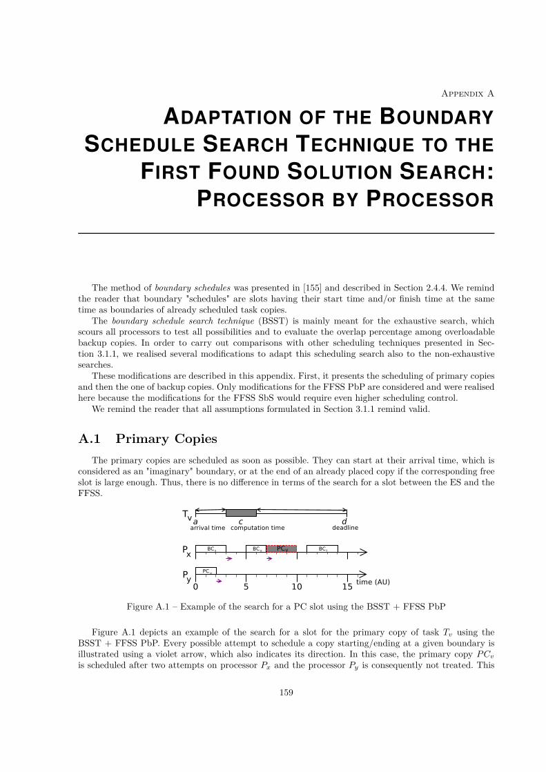
Appendix A

ADAPTATION OF THE BOUNDARY

SCHEDULE SEARCH TECHNIQUE TO THE

FIRST FOUND SOLUTION SEARCH:PROCESSOR BY PROCESSOR

The method of boundary schedules was presented in [155] and described in Section 2.4.4. We remindthe reader that boundary "schedules" are slots having their start time and/or finish time at the sametime as boundaries of already scheduled task copies.

The boundary schedule search technique (BSST) is mainly meant for the exhaustive search, whichscours all processors to test all possibilities and to evaluate the overlap percentage among overloadablebackup copies. In order to carry out comparisons with other scheduling techniques presented in Sec-tion 3.1.1, we realised several modifications to adapt this scheduling search also to the non-exhaustivesearches.

These modifications are described in this appendix. First, it presents the scheduling of primary copiesand then the one of backup copies. Only modifications for the FFSS PbP are considered and were realisedhere because the modifications for the FFSS SbS would require even higher scheduling control.

We remind the reader that all assumptions formulated in Section 3.1.1 remind valid.

A.1 Primary Copies

The primary copies are scheduled as soon as possible. They can start at their arrival time, which isconsidered as an "imaginary" boundary, or at the end of an already placed copy if the corresponding freeslot is large enough. Thus, there is no difference in terms of the search for a slot between the ES and theFFSS.

Figure A.1 – Example of the search for a PC slot using the BSST + FFSS PbP

Figure A.1 depicts an example of the search for a slot for the primary copy of task Tv using theBSST + FFSS PbP. Every possible attempt to schedule a copy starting/ending at a given boundary isillustrated using a violet arrow, which also indicates its direction. In this case, the primary copy P Cv

is scheduled after two attempts on processor Px and the processor Py is consequently not treated. This

159

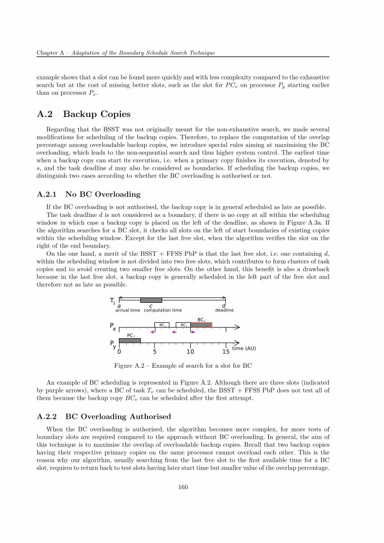
Chapter A – Adaptation of the Boundary Schedule Search Technique

example shows that a slot can be found more quickly and with less complexity compared to the exhaustivesearch but at the cost of missing better slots, such as the slot for P Cv on processor Py starting earlierthan on processor Px.

A.2 Backup Copies

Regarding that the BSST was not originally meant for the non-exhaustive search, we made severalmodifications for scheduling of the backup copies. Therefore, to replace the computation of the overlappercentage among overloadable backup copies, we introduce special rules aiming at maximising the BCoverloading, which leads to the non-sequential search and thus higher system control. The earliest timewhen a backup copy can start its execution, i.e. when a primary copy finishes its execution, denoted bys, and the task deadline d may also be considered as boundaries. If scheduling the backup copies, wedistinguish two cases according to whether the BC overloading is authorised or not.

A.2.1 No BC Overloading

If the BC overloading is not authorised, the backup copy is in general scheduled as late as possible.The task deadline d is not considered as a boundary, if there is no copy at all within the scheduling

window in which case a backup copy is placed on the left of the deadline, as shown in Figure A.3a. Ifthe algorithm searches for a BC slot, it checks all slots on the left of start boundaries of existing copieswithin the scheduling window. Except for the last free slot, when the algorithm verifies the slot on theright of the end boundary.

On the one hand, a merit of the BSST + FFSS PbP is that the last free slot, i.e. one containing d,within the scheduling window is not divided into two free slots, which contributes to form clusters of taskcopies and to avoid creating two smaller free slots. On the other hand, this benefit is also a drawbackbecause in the last free slot, a backup copy is generally scheduled in the left part of the free slot andtherefore not as late as possible.

Figure A.2 – Example of search for a slot for BC

An example of BC scheduling is represented in Figure A.2. Although there are three slots (indicatedby purple arrows), where a BC of task Tv can be scheduled, the BSST + FFSS PbP does not test all ofthem because the backup copy BCv can be scheduled after the first attempt.

A.2.2 BC Overloading Authorised

When the BC overloading is authorised, the algorithm becomes more complex, for more tests ofboundary slots are required compared to the approach without BC overloading. In general, the aim ofthis technique is to maximise the overlap of overloadable backup copies. Recall that two backup copieshaving their respective primary copies on the same processor cannot overload each other. This is thereason why our algorithm, usually searching from the last free slot to the first available time for a BCslot, requires to return back to test slots having later start time but smaller value of the overlap percentage.

160

A.2. Backup Copies

(a) No copy (b) PC(s) only

(c) PC, several BCs until PC (d) PC and several BCs until d

(e) Several BCs and PC (f) BC(s) only

Figure A.3 – Different cases of BC scheduling with BC overloading

In this case, we consider that the start s of the BC scheduling window is never considered as aboundary and that the task deadline d is considered as a boundary:

— if and only if there is no copy at all within the scheduling window and in this case, depicted inFigure A.3a, the algorithm immediately tests the slot on the left;

— if and only if there is no primary copy within the scheduling window, as shown in Figure A.3f,and in this situation it first waits after all backup copies are tested and then, if no slot is found,it tests the slot on the left.

As the BC overloading is authorised, the algorithm distinguishes for each current copy whether aboundary belongs to a primary or backup copy, as it was shown in Figures 3.4.

If a current copy is a primary copy, its end boundary is not tested if there is no copy (Figure A.3b)or no primary copy (Figure A.3d) between the end boundary and d. The algorithm checks the slot onthe right of the boundary.

When the algorithm encounters a start boundary of primary copy, it tests the slot on the left. Thisverification is carried out:

— immediately, if the previous copy is a primary copy (Figure A.3b) or if there is no copy on the leftof the start boundary within the scheduling window;

— after checking all backup copies until previous PC and no slot is found, if the previous copies arethe backup ones on the left of the start boundary within scheduling window (Figures A.3c andA.3e).

The second case is when a current copy is a backup copy. Its start boundary is always takeninto account and the algorithm checks the slot on the right (for instance BCi or BCl in Figures A.3c,A.3d, A.3e and A.3f). The end boundary is not used unless this copy is the first backup copy tested inthe current free slot (for example BCm in Figures A.3c, A.3d, A.3e and A.3f) in which case the algorithmverifies the slot on the left.

An idea to simplify the algorithm when the BC overloading is authorised is to consider only oneboundary of backup copy (start or end one) and thus avoid several special cases.

161

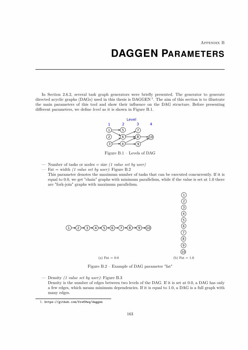
Appendix B

DAGGEN PARAMETERS

In Section 2.6.2, several task graph generators were briefly presented. The generator to generatedirected acyclic graphs (DAGs) used in this thesis is DAGGEN 1. The aim of this section is to illustratethe main parameters of this tool and show their influence on the DAG structure. Before presentingdifferent parameters, we define level as it is shown in Figure B.1.

Figure B.1 – Levels of DAG

— Number of tasks or nodes = size (1 value set by user)— Fat = width (1 value set by user): Figure B.2

This parameter denotes the maximum number of tasks that can be executed concurrently. If it isequal to 0.0, we get "chain" graphs with minimum parallelism, while if the value is set at 1.0 thereare "fork-join" graphs with maximum parallelism.

(a) Fat = 0.0 (b) Fat = 1.0

Figure B.2 – Example of DAG parameter "fat"

— Density (1 value set by user): Figure B.3Density is the number of edges between two levels of the DAG. If it is set at 0.0, a DAG has onlya few edges, which means minimum dependencies. If it is equal to 1.0, a DAG is a full graph withmany edges.

1. https://github.com/frs69wq/daggen

163

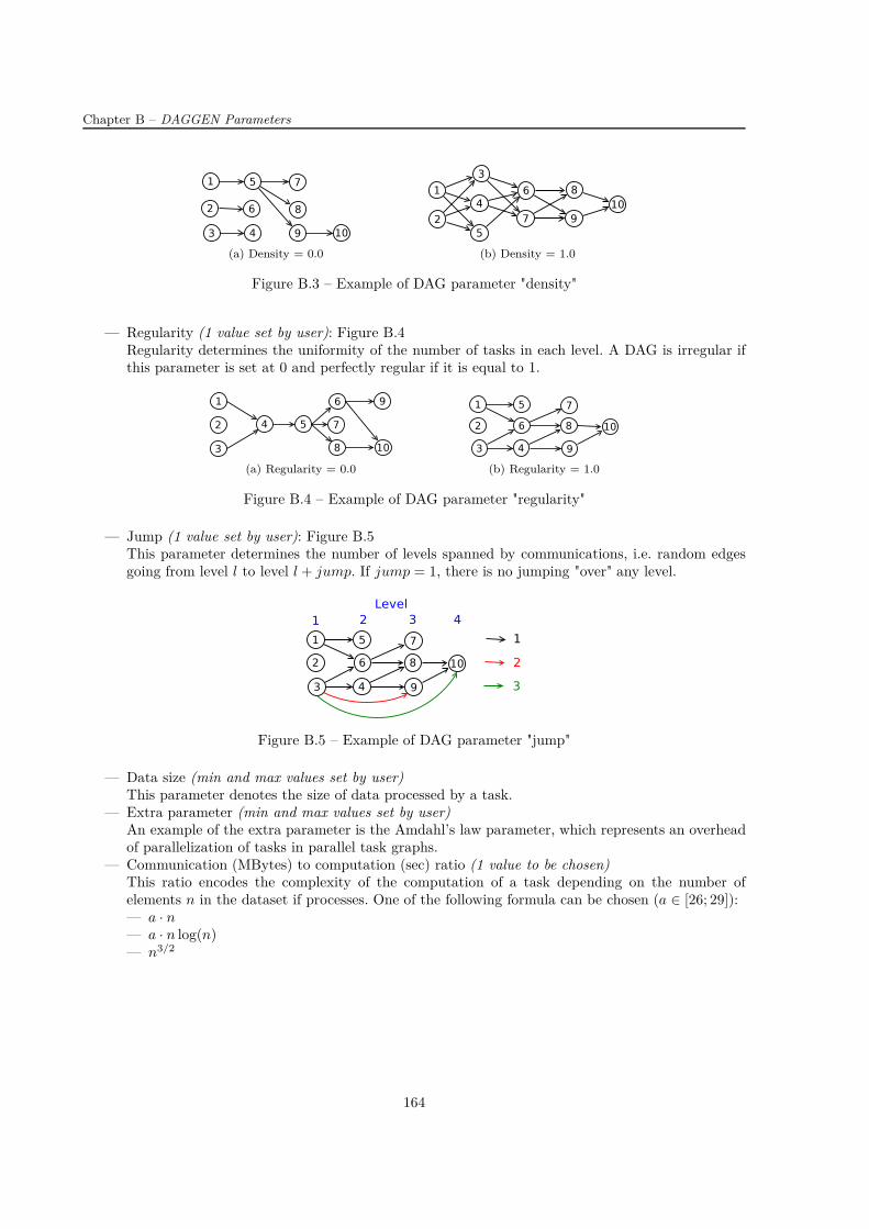
Chapter B – DAGGEN Parameters

(a) Density = 0.0 (b) Density = 1.0

Figure B.3 – Example of DAG parameter "density"

— Regularity (1 value set by user): Figure B.4Regularity determines the uniformity of the number of tasks in each level. A DAG is irregular ifthis parameter is set at 0 and perfectly regular if it is equal to 1.

(a) Regularity = 0.0 (b) Regularity = 1.0

Figure B.4 – Example of DAG parameter "regularity"

— Jump (1 value set by user): Figure B.5This parameter determines the number of levels spanned by communications, i.e. random edgesgoing from level l to level l + jump. If jump = 1, there is no jumping "over" any level.

Figure B.5 – Example of DAG parameter "jump"

— Data size (min and max values set by user)This parameter denotes the size of data processed by a task.

— Extra parameter (min and max values set by user)An example of the extra parameter is the Amdahl’s law parameter, which represents an overheadof parallelization of tasks in parallel task graphs.

— Communication (MBytes) to computation (sec) ratio (1 value to be chosen)This ratio encodes the complexity of the computation of a task depending on the number ofelements n in the dataset if processes. One of the following formula can be chosen (a ∈ [26; 29]):— a · n— a · n log(n)— n3/2

164

Appendix C

CONSTRAINT PROGRAMMING

PARAMETERS

This appendix deals with the settings of some simulation parameters in CPLEX optimiser 1 when solv-ing constraint programming (CP) problems. Actually, when resolving the same problem on two differentcomputational resources, the result may differ because the setting parameters using the default valuesare platform-dependent. Consequently, the model can choose a different solution when there are severalalternate optimal solutions to the problem. In order to reproduce the same results, these parameters needto be set properly [77].

Table C.1 sums up the parameters that were studied during the thesis and have influence on thereproducibility of the results. While the default settings of parameters FailLimit and TimeLimit areindependent of the computational resources, the default setting of the parameter Workers is platform-dependent because its number equals the number of central processing units (CPUs) available.

Table C.1 – Several constraint programming (CP) setting parameters [74, 75, 76]

Parameter Definition Default value

FailLimitLimits the number of failures 2that can

occur before terminating the search2 100 000 000

TimeLimitLimits the CPU time spent solving before

terminating a searchInfinity (s) = 1 · e+75 s

WorkersSets the number of workers to run in

parallel to solve the modelAutomatic (as many workers as

there are CPUs available)

As an example of the influence of the last mentioned parameter, we consider a CubeSat scenario andthe task input consisting of 500 independent tasks. Each task has three copies and dynamically arriveson a 5-processor system. This task data set, which remained exactly the same in all experiments, wasexecuted on a computer composed of four CPUs and on a computing platform equipped with twelve CPUs,while we varied the parameters TimeLimit, FailLimit and Workers. The mathematical formulation ofthe analysed problem is described in Section 5.2.2.1, whose objective function is to maximise the numberof accepted tasks and therefore to minimise the rejection rate.

For every experiment, we measured the time elapsed to find an optimal solution and we recorded therejection rate and processor load of the given solution. The obtained results are encapsulated in Table C.2.

First and foremost, we note that, in order to obtain the same result, the parameter Workers needsto be set at the same value. For example, if TimeLimit =Infinity, FailLimit = 10 000 and Workers = 4,the optimal solution is the same, as highlighted in red.

While it is true for the computing platform that the higher the parameter FailLimit, the lower therejection rate, it is not the case for the computer because the rejection rate when FailLimit = 10 000is higher than when FailLimit = 5 000. It can be also seen that the higher the value of FailLimit,

1. https://www.ibm.com/analytics/cplex-optimizer

2. The number of failures or the number of fails stands for the number of branches explored in the binary search tree,which did not lead to a solution [73].

165

Chapter C – Constraint Programming Parameters

Table C.2 – Example of the influence of parameter settings

TimeLimit FailLimitComputer (# CPUs = 4) Computing platform (# CPUs = 12)

#workers

Rejectionrate

Processorload

Duration(min)

#workers

Rejectionrate

Processorload

Duration(min)

Infinity 5 000 4 0.166 0.876 162 12 0.476 0.538 33.7

Infinity 10 000 4 0.172 0.847 130 4 0.172 0.847 43.7

Infinity 10 000 12 0.112 0.923 44.6

Infinity 15 000 4 0.104 0.927 164 12 0.112 0.923 47.3

Infinity 20 000 4 0.104 0.927 234 12 0.112 0.923 47.3

the longer the time elapsed to find a solution (even though the increase depends on the computationalresources).

We also try not to limit FailLimit. In this case, a CPLEX optimiser treated only the first 22 arrivedtasks within the first 30 minutes of simulation (no matter whether a computer or computing platform wasused). The simulations were then stopped because the duration exponentially increases with the numberof tasks and the time to find an optimal solution would be too long if a simulation would finish at all.

Therefore, the value of FailLimit to be chosen for simulations is the value that corresponds to thefirst case when studied metrics do not vary any more when the parameter FailLimit increases on a givencomputational resource (marked by green and blue in Table C.2). In the studied case, FailLimit equals10 000 for the computing platform and 15 000 for the computer.

Furthermore, if the value of FailLimit is too low, the rejection rate may be very high, e.g. 0.476 forthe computing platform with FailLimit = 5 000 and 12 workers.

We notice that it is useless to limit TimeLimit because presented results finish in reasonable timeand that, although the resolutions are carried out faster when the number of CPUs increases, the highernumber of CPUs available does not mean that the results will be better. In the analysed example, therejection rate of the optimal solution of the computing platform (0.112) is higher by 7.7% comparedto the one delivered by the computer (0.104). This is caused by a different decision made when severalalternate optimal solutions to the problem are available [77].

Throughout this thesis, the parameter TimeLimit was kept to the default value and the parameterFailLimit was fixed at 10 000 for all conducted resolutions in CPLEX optimiser. While the problemoptimisations for the primary/backup approach were realised on a computing platform equipped with 12CPUs, the one for CubeSats were conducted on a computer composed of 4 CPUs.

166

Appendix D

BOX PLOT

The box plot, also known as the box-and-whisker plot, is a histogram-like method invented by JohnWilder Tukey [43, 98, 113, 150]. This graphical tool is used to represent statistical data, in particulartheir location and variation information. An example of a box plot is depicted in Figure D.1. A diagramhas two or three parts, which are as follows: box, whiskers and circle(s).

Figure D.1 – Example of a box plot

Before explaining the meaning of each part, we give several definitions.— A quartile is one of the four divisions of data set and it splits this data set into four equal parts.

The first quartile Q1 is called lower quartile value and corresponds to the 25th percentile. Thethird quartile, named upper quartile value, is the 75th percentile.

— The median is the value of the point which is situated in the middle of the data set. It means thatone half has the data smaller than this point and another half has the data larger than this point.If the number of data is odd, the median value is included in both halves.

— The interquartile range (IQR) is the difference between the third and the first quartiles, i.e. IQR =Q3 − Q1. This interval divides a data set into two groups of equal size at the median.

The box is respectively delimited by the first and third quartiles Q1 and Q3. A horizontal line in thebox represents the statistical median M .

The whiskers start at the end of the box and extend to the outermost points that are not outliers,which means that they are within 1.5 times the interquartile range of Q1 and Q3.

The circle represents an outlier for a studied data set. An outlier is a value that is more than 1.5times the interquartile range from the end of a box.

167

PUBLICATIONS

P. Dobiáš, E. Casseau, and O. Sinnen, Restricted Scheduling Windows for Dynamic Fault-Tolerant Primary/Backup Approach-Based Scheduling on Embedded Systems, in Proceedings of the 21stInternational Workshop on Software and Compilers for Embedded Systems, SCOPES ’18, May 2018, pp.27–30. https://doi.org/10.1145/3207719.3207724.

P. Dobiáš, E. Casseau, and O. Sinnen, Comparison of Different Methods Making Use of BackupCopies for Fault-Tolerant Scheduling on Embedded Multiprocessor Systems, in 2018 Conference on Designand Architectures for Signal and Image Processing (DASIP), Oct 2018, pp. 100–105. https://doi.org/

10.1109/DASIP.2018.8597044.

P. Dobiáš, E. Casseau, and O. Sinnen, Fault-Tolerant Online Scheduling Algorithms for CubeSats,in Proceedings of the 11th Workshop on Parallel Programming and Run-Time Management Techniquesfor Many-Core Architectures / 9th Workshop on Design Tools and Architectures for Multicore Embed-ded Computing Platforms, PARMA-DITAM’2020, January 2020, pp. 1–6. https://doi.org/10.1145/

3381427.3381430.

P. Dobiáš, E. Casseau, and O. Sinnen, Evaluation of Fault Tolerant Online Scheduling Algorithmsfor CubeSats, in Proceedings of the 23rd Euromicro Conference on Digital System Design, DSD’2020,August 2020, pp. 622–629. https://doi.org/10.1109/DSD51259.2020.00102.

169

BIBLIOGRAPHY

[1] Live Real Time Satellite Tracking and Predictions. https://www.n2yo.com/.

[2] Documentation of AAU-Cubesat On Board Computer Software, 2002. Aalborg University http://

www.space.aau.dk/cubesat/dokumenter/software.pdf.

[3] PW-SAT 2 Preliminary Requirements Review: On-Board Computer, 2014. WarsawUniversity of Technology https://pw-sat.pl/wp-content/uploads/2014/07/PW-Sat2-A-04.

00-OBC-PRR-EN-v1.1.pdf.

[4] K. Ahn, J. Kim, and S. Hong, Fault-tolerant real-time scheduling using passive replicas, inProceedings Pacific Rim International Symposium on Fault-Tolerant Systems, Dec 1997, pp. 98–103. https://doi.org/10.1109/PRFTS.1997.640132.

[5] R. Al-Omari, A. K. Somani, and G. Manimaran, A New Fault-Tolerant Technique for Improv-ing Schedulability in Multiprocessor Real-Time Systems, in Proceedings 15th International Paralleland Distributed Processing Symposium (IDPS), 2001. https://doi.org/10.1109/IPDPS.2001.

924967.

[6] R. Al-Omari, A. K. Somani, and G. Manimaran, Efficient Overloading Techniques forPrimary-Backup Scheduling in Real-Time Systems, in Journal of Parallel and Distributed Com-puting, vol. 64, 2004, pp. 629–648. https://doi.org/10.1016/j.jpdc.2004.03.015.

[7] S. Al-Sharaeh and B. E. Wells, A Comparison of Heuristics for List Schedules using theBox-Method and P-Method for Random Digraph Generation, in Proceedings of 28th SoutheasternSymposium on System Theory, 1996, pp. 467–471. https://doi.org/10.1109/SSST.1996.493549.

[8] V. Almonacid and L. Franck, Extending the Coverage of the Internet of Things with Low-CostNanosatellite Networks, in Acta Astronautica, vol. 138, 2017, pp. 95–101. https://doi.org/10.

1016/j.actaastro.2017.05.030.

[9] A. Amin, R. Ammar, and A. El Dessouly, Scheduling real time parallel structures on clustercomputing with possible processor failures, in Proceedings. ISCC 2004. Ninth International Sympo-sium on Computers And Communications (IEEE Cat. No.04TH8769), vol. 1, July 2004, pp. 62–67.https://doi.org/10.1109/ISCC.2004.1358382.

[10] K. Anderson, Low-Cost, Radiation-Tolerant, On-Board Processing Solution, in IEEE AerospaceConference, March 2005, pp. 1–8. https://doi.org/10.1109/AERO.2005.1559533.

[11] K. Antonini, M. Langer, A. Farid, and U. Walter, SWEET CubeSat – Water Detection andWater Quality Monitoring for the 21st Century, in Acta Astronautica, vol. 140, 2017, pp. 10–17.https://doi.org/10.1016/j.actaastro.2017.07.046.