One-loop effective potential on hyperbolic manifolds

arX

iv:h

ep-t

h/93

0205

1v1

12

Feb

1993

One-loop effective potential on hyperbolic manifolds

Guido Cognola∗, Klaus Kirsten and Sergio Zerbini∗

Dipartimento di Fisica, Universita di Trento, Italia†

February 1993

U.T.F. 284

Abstract: The one-loop effective potential for a scalar field defined on an ultrastatic

space-time whose spatial part is a compact hyperbolic manifold, is studied using

zeta-function regularization for the one-loop effective action. Other possible regu-

larizations are discussed in detail. The renormalization group equations are derived

and their connection with the conformal anomaly is pointed out. The symmetry

breaking and the topological mass generation are also discussed.

PACS numbers: 03.70.+k Theory of quantized fields

11.10.Gh Renormalization

04.90.+e Other topics in relativity and gravitation

1 Introduction

In the last decades, there has been a great deal of investigations on the properties of

interacting quantum field theories in curved space-time (see for example the text book [1]

∗Istituto Nazionale di Fisica Nucleare, Gruppo Collegato di Trento, Italia

†Email: [email protected], [email protected], [email protected]

1

and references cited therein). More recently the inflationary models have been proposed

in order to overcome some difficulties present in the standard cosmological model (see

for example [2] and references therein). Several techniques have been employed, among

these the background-field method within path-integral approach to quantum field theory

[3, 4], which is very useful in dealing with the one-loop approximation. In addition there

have been attemps to investigate the role of the topology and the phenomenon of the

topological mass generation has been discovered [5, 6, 7, 8]. Furthermore ”topological

symmetry restoration” [9, 10, 11] and later ”topological symmetry breaking” [12, 13]

have been investigated in the self-interacting scalar theory. The non trivial topological

space-times which mainly have been considered are the ones with the torus topology, with

the exception of ref. [11], in which untwisted scalar fields on S3/Γ are discussed (Γ is a

discrete group of isometries of S3). Very recently, such manifolds have been considered

also by Dowker et al. [14].

In this paper we shall consider a self-interacting scalar field defined on an ultrastatic

space-time in which the spatial section is a compact hyperbolic 3-dimensional manifold,

namely it can be represented as H3/Γ, Γ being a discrete group of isometries of H3, the

Lobachevsky space. It is well known that such space-times have a highly non trivial topol-

ogy and, for a fixed value of cosmological time, they are spatially homogeneous isotropic

universe models with negative constant curvature. It is reasonable to assume that such

space-times have some physical relevance. In fact, as it has been stressed in ref. [15], they

would affect the occurence of the particle horizons and in principle they could be tested

experimentally by means of observation. There is also a mathematical motivation based

on the Thurston conjecture [16] which, roughly speaking, states that every 3-dimensional

compact manifold admits a canonical decomposition into eight primitive pieces. Among

2

such primitive pieces, the hyperbolic one is the most important, the other contributions

being exceptional cases. As a consequence, if one is interested in studying matter fields

defined on space-times with a compact spatial section, the compact hyperbolic case might

play an important physical role. In fact one of the results achieved in this paper is an

expression for the square of the topological mass. The sign of this depends on the char-

acters of the fields. For trivial character (untwisted fields) the sign is positive (this might

help to restore symmetry) whereas for twisted fields there could exist a mechanism for

symmetry breaking.

The plan of the paper is the following. In Section 2, the scalar model is introduced

and the definition of the regularized one-loop effective potential within the background

field method is summarized. It is also shown that the finite part of the one-loop effective

potential in RD can be determined without the explicit knowledge of the regularization

functions. In Section 3, making use of the Selberg trace formula, the one-loop effective

potential for R×H3/Γ is computed. In Section 4, the renormalization program is carried

out. In Section 5 a derivation of the renormalization group equations at one-loop level

is presented for the sake of completeness, paying attention to the role of the conformal

anomaly. In Section 6, symmetry breaking and topological mass generation are discussed.

The conclusions are summarized in Section 7. In Appendix A, several regularizations are

discussed in order to illustrate the general result obtained in Section 2. Finally, Appendix

B contains some material on heat kernel expansion and zeta-function regularization.

3

2 One loop-effective potential

Before we restrict our attention to the hyperbolic manifold R × H3/Γ, let us deal with

a scalar field φ defined on an arbitrary smooth D-dimensional manifold M (Euclidean

signature), for simplicity without boundary. To begin with, we recall that the Euclidean

generating functional reads

WE [J ] = NE

∫

d[φ]e−SE [φ,J ] (2.1)

where

SE [φ, J ] =∫

M

[

12φLφ+ Vo(φ) − Jφ

]

dvol (2.2)

L = −△D +m2 + ξR (2.3)

Here △D is the Laplace-Beltrami operator in M, R is the scalar curvature, ξ an arbitrary

numerical parameter and finally Vo(φ) is the potential describing the self-interaction of

the field.

If we denote the classical solution by φc, the one loop effective action takes the form

Γ[φc] = SE [φc] + 12ln det A

µ2 = SE[φc] + 12ln det L+V ′′

o (φc)µ2

=∫

[

V (φc) + 12Z(φc)g

ij∂iφc∂jφc + · · ·]

dvol (2.4)

in which A is a positive definite elliptic operator of second order defined on M (the

small disturbance or fluctuation operator) and µ is an arbitrary normalization parameter

coming from the scalar path-integral measure and necessary in order to keep the zeta-

function dimensionless for all s. The latter equation defines the one-loop effective potential

V (φc). Of course it is equal to the classical one V (0)(φc) = Vo(φc) + (m2 + ξR)φ2c/2, plus

4

quantum corrections V (1)(φc) of order h. The quantum corrections to the classical action

are formally divergent, because the eigenvalues of A increase without bound. One has to

use a suitable regularization procedure.

In the following we shall employ a class of regularizations based on the Schwinger

representation (see for example [17]). In order to work with dimensionless quantities, we

put B = µ−2A. The regularized determinant of the operator B is defined by

(ln detB)ε = −∫ ∞

0dt t−1(ε, t) Tr e−tB (2.5)

where (ε, t) is a suitable regularization function of the dimensionless parameter t, which

has to satisfy the two requirements we are going to discuss. First, for fixed t > 0, the

limit as ε goes to zero must be equal to one. Second, for fixed and sufficiently large ε,

(ε, t) has to regularize the singularity at t = 0 coming from the heat kernel expansion

Tr e−tB ∼∑

n

Antn−D/2 (2.6)

An being the integrated Seeley-DeWitt coefficients associated with the operator B. The

analytic continuation will be used to reach small values of ε. These requirements do

not uniquely determine the regularization function . In fact, in the following we shall

examine several cases.

Using eq. (2.6) in eq. (2.5) one can easily see that the number of divergent terms

for ε → 0 is equal to Q + 1, Q being the integer part of D/2. They are proportional

to the Seeley-De Witt coefficients A0, . . . AQ (which contain the full dependence on the

geometry), the prefactors depending on the regularization function [17]. In the Appendix

A, this general result is verified explicitly in several examples.

In the rest of this Section, in the particular but important case of RD, we would like

to show that the finite part of the effective potential is uniquely determined, modulo a

5

constant which can be absorbed by the arbitrary scale parameter µ, and can be evaluated

without making use of the explicit knowledge of the regularization functions . As usual,

in RD we consider a large region of volume V (M) and the limit V (M) → ∞ shall

be taken at the end of the calculations. As we will see in the following section, apart

from a topological contribution which will be obtained using the Selberg trace formula,

this calculation is already enough to give the one loop-effective potential in the constant

curvature space-time R×H3/Γ under consideration.

By definition, the effective potential has to be evaluated by considering a constant V ′′o .

This means that

Tr e−tB

V (M)=µDe−tf2/µ2

(4πt)D/2(2.7)

where f 2 = m2 + V ′′o (φc) is a positive constant. As a consequence, from eqs. (2.4) and

(2.5), we obtain the regularized expression V (ε, f) for V (1)(φc),

V (ε, f) =(ln detB)ε

2V (M)= −1

2

(

µ2

4π

)D/2∫ ∞

0dt t−(1+D/2)(ε, t)e−tf2/µ2

(2.8)

Now it is convenient to distinguish between even (D = 2Q) and odd (D = 2Q + 1)

dimensions. In order to derive a more explicit form of the divergent terms for ε → 0, let

us consider the Qth-derivative of V (ε), which is

dQV (ε, f)

dyQ=

(−1)Q

2

(

µ2

4π

)D/2

Be,o(ε, y) (2.9)

where

Be(ε, y) = −∫ ∞

0dt t−1(ε, t)e−ty = ln y + b+ cQ(ε) + O(ε) (2.10)

Bo(ε, y) = −∫ ∞

0dt t−3/2(ε, t)e−ty = 2

√πy + b+ cQ(ε) + O(ε) (2.11)

6

In the derivation of the above equations we have made use of the properties of the regu-

larization functions. Furthermore, in eqs. (2.10) and (2.11) b is a constant and cQ(ε) is a

function of ε, but not of y. We have used the same symbols for even and odd dimensions,

but of course they represent different quantities in the two cases.

Making use of eqs. (2.10) and (2.11) in eq. (2.9) a simple integration gives

V2Q(ε, f) =(−1)Q

2Q!(4π)Q

[

ln f2

µ2 − CQ + b]

fD + µDQ∑

n=0

cn(ε)(

fµ

)2n+ O(ε) (2.12)

V2Q+1(ε, f) =(−1)QΓ(−Q− 1/2)

2(4π)Q+1/2fD + µD

Q∑

n=0

cn(ε)(

fµ

)2n+ O(ε) (2.13)

where we have set CQ =∑Q

n=11n.

The dimensionless integration constants cn(ε), which are divergent for ε → 0, define

the counterterms which must be introduced in order to remove the divergences. For the

particularly interesting case D = 4 one gets

V (ε, f) =f 4

64π2

[

ln f2

µ2 − 32

+ b]

+ c2(ε)f4 + c1(ε)µ

2f 2 + c0(ε)µ4 (2.14)

in agreement with the well known result obtained in refs. [18, 19], where some specific

regularizations were used for D = 4.

Some remarks are in order. The constants b and cn(ε) depend on the choice of the

regularization function, but b can be absorbed by the arbitrary scale parameter µ. As a

result, the finite part of the effective potential does not depend on the regularization, as

expected. In the Appendix A, several examples of admissible regularizations are reported

as an illustration of the above general result.

7

3 The effective potential on R×H3/Γ

In the following we shall consider the scalar field defined on a topologically non trivial

space-time R ×HD−1/Γ, that is a space-time with a hyperbolic N = D − 1 dimensional

manifold as a compact spatial part and with constant scalar curvature R = N(N − 1)κ.

Note that R is also the scalar curvature of HN . We shall explicitly compute the effective

potential only for the physical interesting case N = 3, but the extension to any N is

possible.

The manifold HN/Γ can be regarded as a quotient of the Lobachevsky space HN by a

fixed-point free discontinuous group Γ of isometries. The Γ is assumed to be torsion-free.

As usual, for the moment we will consider the case normalized to κ = −1, so until not

otherwise stated all quantities are dimensionless. The results for arbitrary κ are simply

found by dimensional reasoning because HN/Γ is a homogeneous manifold.

If h(r) is an even and holomorphic function in a strip of width N about the real axis,

and if h(r) = O(r−(N+1+ε)) uniformly in this strip as r → ∞, then the Selberg trace

formula holds (see for example refs. [20, 21])

∞∑

j=0

h(rj) = V (F)∫ ∞

0drh(r)ΦN(r) +

∑

℘

∞∑

n=1

χ(P n(γ))

SN(n; lγ)h(nlγ) (3.1)

Here V (F) is the volume of the fundamental domain F , h is the Fourier transform of h,

γ ∈ Γ is an element of the conjugacy class associated with the length of a closed geodesic

lγ , ℘ is a set of primitive closed geodesics on the compact manifold and each γ ∈ ℘

determines the holonomy element P (γ). Moreover, SN(n; lγ) is a known function of the

conjugacy class (see ref. [22] for details) and χ(P ) represents the characters, which define

all topological inequivalent scalar fields. The sum on the left hand side of eq. (3.1) is over

8

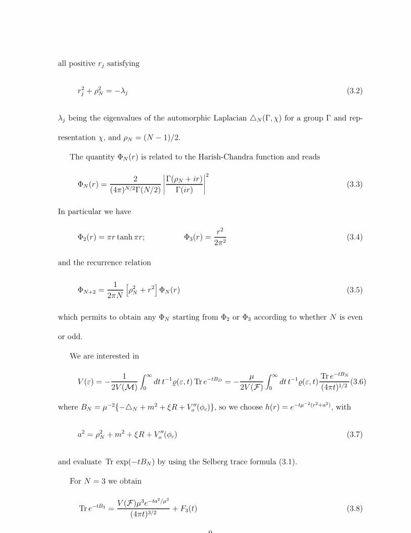
all positive rj satisfying

r2j + ρ2

N = −λj (3.2)

λj being the eigenvalues of the automorphic Laplacian △N(Γ, χ) for a group Γ and rep-

resentation χ, and ρN = (N − 1)/2.

The quantity ΦN (r) is related to the Harish-Chandra function and reads

ΦN (r) =2

(4π)N/2Γ(N/2)

∣

∣

∣

∣

∣

Γ(ρN + ir)

Γ(ir)

∣

∣

∣

∣

∣

2

(3.3)

In particular we have

Φ2(r) = πr tanh πr; Φ3(r) =r2

2π2(3.4)

and the recurrence relation

ΦN+2 =1

2πN

[

ρ2N + r2

]

ΦN(r) (3.5)

which permits to obtain any ΦN starting from Φ2 or Φ3 according to whether N is even

or odd.

We are interested in

V (ε) = − 1

2V (M)

∫ ∞

0dt t−1(ε, t) Tr e−tBD = − µ

2V (F)

∫ ∞

0dt t−1(ε, t)

Tr e−tBN

(4πt)1/2(3.6)

where BN = µ−2{−△N +m2 + ξR+ V ′′o (φc)}, so we choose h(r) = e−tµ−2(r2+a2), with

a2 = ρ2N +m2 + ξR+ V ′′

o (φc) (3.7)

and evaluate Tr exp(−tBN ) by using the Selberg trace formula (3.1).

For N = 3 we obtain

Tr e−tB3 =V (F)µ3e−ta2/µ2

(4πt)3/2+ F3(t) (3.8)

9

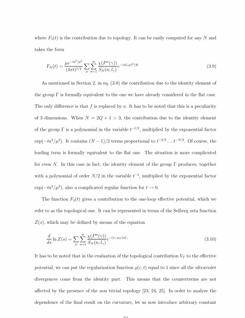
where F3(t) is the contribution due to topology. It can be easily computed for any N and

takes the form

FN(t) =µe−ta2/µ2

(4πt)1/2

∑

℘

∞∑

n=1

χ(P n(γ))

SN(n; lγ)e−(nlγµ)2/4t (3.9)

As mentioned in Section 2, in eq. (3.8) the contribution due to the identity element of

the group Γ is formally equivalent to the one we have already considered in the flat case.

The only difference is that f is replaced by a. It has to be noted that this is a peculiarity

of 3 dimensions. When N = 2Q + 1 > 3, the contribution due to the identity element

of the group Γ is a polynomial in the variable t−1/2, multiplied by the exponential factor

exp(−ta2/µ2). It contains (N − 1)/2 terms proportional to t−3/2 . . . t−N/2. Of course, the

leading term is formally equivalent to the flat one. The situation is more complicated

for even N . In this case in fact, the identity element of the group Γ produces, together

with a polynomial of order N/2 in the variable t−1, multiplied by the exponential factor

exp(−ta2/µ2), also a complicated regular function for t→ 0.

The function F3(t) gives a contribution to the one-loop effective potential, which we

refer to as the topological one. It can be represented in terms of the Selberg zeta function

Z(s), which may be defined by means of the equation

d

dslnZ(s) =

∑

℘

∞∑

n=1

χ(P n(γ))

SN(n; lγ)e−(s−ρN )nlγ (3.10)

It has to be noted that in the evaluation of the topological contribution VT to the effective

potential, we can put the regularization function (ε, t) equal to 1 since all the ultraviolet

divergences come from the identity part. This means that the counterterms are not

affected by the presence of the non trivial topology [23, 24, 25]. In order to analyze the

dependence of the final result on the curvature, let us now introduce arbitrary constant

10

curvature R. Then we have lγ ∼ 1/√

|κ|, V (F) ∼ |κ|− 3

2 , furthermore a2 = m2 + (ξ −

1/6)R + V ′′o (φc), and we find V (ε) = V (ε, a) + VT , V (ε, a) being given in eq. (2.12) with

Q = 2 and

VT = −a2|κ|−1/2

2πV (F)

∑

℘

∞∑

n=1

χ(P n(γ))

S3(n; lγ)

K1(nlγa)

nlγa(3.11)

From the latter equation we can see that for a > 0, VT is exponentially vanishing when κ

goes to zero due to the fact that lγ diverges as |κ|−1/2 when κ→ 0.

Making use of a suitable integral representation for K1 [26] and definition (3.10) we

may write VT in the final form

VT = −a2|κ|−1/2

2πV (F)

∫ ∞

1du

√u2 − 1

Z ′

Z(1 + ua|κ|−1/2) (3.12)

in agreement with the zeta-function calculation [27].

4 Renormalization of λφ4 on R×H3/Γ

In the previous section we have derived the regularized one-loop effective potential V (φc, R) =

V (0)(φc, R) + V (1)(φc, R) for a scalar field defined on the manifold R × H3/Γ. We now

introduce R into the notation to remind the reader of the nonvanishing curvature. The

one-loop effective potential depends on the arbitrary parameter µ, this dependence being

eliminated by the renormalization procedure. To this aim, here we consider a scalar field

self-interacting by a term of the kind Vo(φ) = λφ4/24 and consider the classical potential

Vc(φc, R)) = Λ +λφ4

c

24+m2φ2

c

2+ξRφ2

c

2+ ε0R +

ε1R2

2(4.1)

Λ being the cosmological constant. Note that one is forced to take into consideration the

most general quadratic gravitational Lagrangian, because the renormalization procedure

gives rise in a natural manner to all such terms in the curvature [28].

11

We write the renormalized one-loop effective potential in the form

Vr(φc, R) = Vc(φc, R) + V (1)r (φc, R) (4.2)

where

V (1)r (φc, R)) =

a4

64π2

[

ln a2

µ2 − 32

]

+ VT (φc, R) + δV (φc, R) (4.3)

with the counterterm contribution

δV (φc, R) = δΛ +δλφ4

c

24+δm2φ2

c

2+δξRφ2

c

2+ δε0R +

δε1R2

2(4.4)

reflecting the structure of the divergences.

For convenience now we indicate by α = αq (q = 0, . . . , 5) the collection of the coupling

constants, that is (α0, . . . , α5) ≡ (Λ, λ,m2, ξ, ε0, ε1). The quantities δα, which renormalize

the coupling constants, are determined by the following renormalization conditions [29, 30]

Λ = Vr|φc=ϕ0,R=0 ; λ = ∂4Vr

∂φ4c

∣

∣

∣

φc=ϕ1,R=R1

; m2 = ∂2Vr

∂φ2c

∣

∣

∣

φc=0,R=0;

ξ = ∂3Vr

∂R∂φ2c

∣

∣

∣

φc=ϕ3,R=R3

; ε0 = ∂Vr

∂R

∣

∣

∣

φc=0,R=0; ε1 = ∂2Vr

∂R2

∣

∣

∣

φc=ϕ5,R=R5

.

(4.5)

By ϕ0 we indicate the value of the field for which the potential has a true minimum. For

m2+ξR > 0 (respectively m2+ξR < 0) this value is zero (respectively ±(−6[m2+ξR]/λ)1

2 )

for the classical potential, but this may change for the one-loop effective one. The choice

of different values φc = ϕq and R = Rq in order to define the physical coupling constants

is due to the fact that in general they are measured at different scales, the behaviour with

respect to a change of scale being determined by the renormalization group eqs. (5.9),

which we shall derive in the next Section. It has to be noted that by a suitable choice

of ϕq and Rq, equations (4.5) reduce to the conditions chosen by other authors (see for

example refs. [29] and [30]).

12

By imposing conditions (4.5) we obtain the counterterms (we used an algebraic com-

puting program)

δΛ = −m2ϕ2

0

2− λϕ4

0

24+∂4VT (ϕ1, R1)

∂φ4c

ϕ40

24+

1

64π2

[

M40

(

32− ln

M2

0

µ2

)

−λm2ϕ20

(

1 − ln m2

µ2

)

+λ2ϕ4

0

12

(

3 lnM2

1

µ2 +6λϕ2

1

M21

− λ2ϕ41

M41

)]

δλ = − λ2

32π2

[

3 lnM2

1

µ2 +6λϕ2

1

M21

− λ2ϕ41

M41

]

− ∂4VT (ϕ1, R1)

∂φ4c

δm2 =λm2

32π2

[

1 − ln m2

µ2

]

(4.6)

δξ = −λ(ξ − 1/6)

32π2

[

lnM2

3

µ2 +λϕ2

3

M2

3

]

− ∂3VT (ϕ3, R3)

∂φ2c∂R

δε0 =(ξ − 1/6)m2

32π2

[

1 − ln m2

µ2

]

δε1 = −(ξ − 1/6)2

32π2ln

M2

5

µ2 − ∂2VT (ϕ5, R5)

∂R2

where the fact that the topological contribution VT (φc, R) to the effective potential is ex-

ponentially vanishing for R → 0 has been used in writing the latter expressions. Moreover,

we have set

M2q = a2(ϕq, Rq) = m2 + (ξ − 1

6)Rq +

λϕ2q

2(4.7)

The final expression for the renormalized one-loop effective potential does not depend

on the arbitrary scale parameter µ. We have

V (1)r (φc, R) = −m

2ϕ20

2− λϕ4

0

24+

λ2φ4c

256π2

[

(

ln a2

M2

1

− 256

)

+4m2(m2 +M2

1 )

3M41

]

+λφ2

c

64π2

[

(ξ − 16)R(

ln a2

M2

3

− 32− λϕ2

3

M2

3

)

+m2(

ln a2

m2 − 12

)]

+1

64π2

[

2m2(ξ − 16)R(

ln a2

m2 − 12

)

+ (ξ − 16)2R2

(

ln a2

M2

5

− 32

)

+m4 ln a2

M2

0

− λm2ϕ20

(

lnM2

0

m2 − 12

)

(4.8)

13

−λ2ϕ4

0

4

(

lnM2

0

M2

1

− 32− 4(M2

1−m2)(2M2

1+m2

3M4

1

)

]

+VT (φc, R) +∂4VT (ϕ1, R1)

∂φ4c

(

φ4c − ϕ4

0

24

)

−∂3VT (ϕ3, R3)

∂φ2c∂R

Rφ2c

2− ∂2VT (ϕ5, R5)

∂R2

R2

2

Expression (4.8) notably simplifies in the special but important case of a conformal

invariant scalar field. First of all we observe that the scalar curvature of a manifold of

the kind R×HN/Γ is just the same as one has for HN . This means that R = N(N − 1)κ

and

a2 = m2 + {ξ − (D − 2)/4(D − 1)}R + V ′′o (φc) (4.9)

Then we see that for a conformally coupled scalar field, a2 = λφ2c/2 does not depend on

the curvature. One easily gets

V (1)r (φc, R) =

λ2φ4c

256π2

[

ln φ2c

ϕ2

1

− 256

]

− λ2ϕ40

256π2

[

lnϕ2

0

ϕ2

1

− 256

]

− λϕ40

24+ VT (φc, R)

+∂4VT (ϕ1, R1)

∂φ4c

(

φ4c − ϕ4

0

24

)

− ∂3VT (ϕ3, R3)

∂φ2c∂R

Rφ2c

2(4.10)

which reduces to the potential of Coleman-Weinberg [18] in the flat space limit.

5 The renormalization group equations for λφ4

In the present section we derive the renormalization group equations for the λφ4 theory

[31] on a 4-dimensional compact smooth manifold without boundary, the extension to

manifolds with boundary being straightforward. The derivation is presented only for the

sake of completeness and is valid only at one-loop level. For a more general discussion see

for example [32] and references cited therein.

14

It is convenient to regularize the one-loop effective action (2.4) by means of the zeta-

function technique [33]. In this way the one-loop effective action is finite and reads

Γ[φc, g] = Sc[φc, g] +12ζ ′(0;A/µ2) =

∫

L √g d4x (5.1)

where ζ ′(s;A/µ2) is the derivative of the zeta-function related to the small disturbance

operator A = L+ λφ2c/2. The classical action is assumed to be of the form

Sc[φc, g] =∫

[

φcLφc

2+λφ4

c

24

]

√gd4x+

∫

[

Λ + ε0R +ε1R

2

2+ ε2C

2

]

√gd4x (5.2)

C2 = CijrsCijrs being the square of the Weyl tensor. Note however that C2 = 0 on the

manifold under consideration and so such a term has been omitted in the previous section.

In order to see how the conformal anomaly enters into the game, we consider a con-

formal transformation gij = exp(2σ)gij with σ a constant (scaling). By the conformal

transformation properties of the fields, one can easily check that Sc(α) = Sc(α), where as

before α represents the collection of all coupling constants and α are all equal to α apart

from Λ, m2, and ε0. For these we have

Λ = Λe4σ; m2 = m2e2σ; ε0 = ε0e2σ. (5.3)

In the same way, for the eigenvalues µn(α) of the small disturbance operator A(α) we have

µn(α) = e−2σµn(α). From this transformation rule for the eigenvalues, we immediately

get the transformations for ζ(s;A/µ2) and ζ ′(s;A/µ2). They read

ζ(s; A/µ2) = e2sσζ(s;A(α)/µ2)

ζ ′(s; A/µ2) = e2sσ[

ζ ′(s;A(α)/µ2) + 2σζ(s;A(α/µ2)]

(5.4)

15

and finally

Γ(α) = Γ(α) − σζ(0;A(α)) (5.5)

It is well known that ζ(0;A) is related to the Seeley-DeWitt coefficient aD/2(x;A) by

means of the equation

ζ(0;A) =1

(4π)D/2

∫

aD/2(x;A)√gdDx (5.6)

(see the Appendix B for details on zeta-function and heat kernel expansion). What is

relevant for our case is a2(x;A(α)) which is known to be [34, 35]

a2(x;A(α)) = −λ△φ2c

12+λm2φ2

c

2+λ(ξ − 1/6)Rφ2

c

2+λ2φ4

c

8+m4

2

+m2(ξ − 16)R +

(ξ − 1/6)2R2

2+C2

120− G

360+

(5 − ξ)△R6

(5.7)

where G = RijrsRijrs − 4RijRij +R2 is the Gauss-Bonnet density, which is a total diver-

gence in 4 dimensions. Integrating a2 on the manifold and disregarding all total diver-

gences one finally gets

Γ(α) = Sc(α(σ)) +1

2ζ ′(0; A) = Γ(α(σ)) + o(h2) (5.8)

The new parameters α(σ) are related to the old ones α = α(0) by

Λ(σ) − Λ = m4

2σ; λ(σ) − λ = 3λ2σ; m2(σ) −m2 = λm2σ;

ξ(σ) − ξ = (ξ − 16)λσ; ε0(σ) − ε0 = (ξ − 1

6)m2σ; ε1(σ) − ε1 = (ξ − 1

6)2σ;

ε2(σ) − ε2 = 130σ.

(5.9)

Here we have set σ = −σ/16π2. With the substitution σ → −2τ , the latter equations

have been given for example in refs. [36, 29]. These important formulae tell us that all

16

parameters (coupling constants) develop as a result of quantum effects a scale dependence

even if classically they are dimensionless parameters. This means that in the quantum

case we have to define the coupling constants at some particular scale. Differentiating

eq. (5.9) with respect to σ, one immediately gets the renormalization group equations

[36, 29].

6 Symmetry breaking and topological mass genera-

tion

Let us now concentrate on the physical implications of the one-loop effective poten-

tial, eq. (4.8). In order to analyze the phase transition of the considered system, let

us specialyze to different cases and to several limits. For this discussion, we will consider

R1 = R3 = R5 = 0. In this way, for q = 1, 3, 5 we have M2q = m2 + λϕ2

q/2.

Let us first concentrate on the regime m2 + ξR > 0. Then φc = 0 is a minimum of

the classical potential and the expansion of the quantum corrections around the classical

minimum reads

Vr = Λeff +(m2 + ξR+m2

T )φ2c

2+

λφ2c

64π2

[

m2 ln m2+(ξ−1/6)Rm2

+R(

ξ − 16

) (

ln m2+(ξ−1/6)RM2

3

− λϕ2

3

M2

3

− 1)]

+ O(φ4c) (6.1)

where Λeff (the effective cosmological constant) represents a complicated expression not

depending on the background field φc and m2T is the topological contribution to the mass

of the field, which reads

m2T =

√3λ|R|−1/2

4πV (F)

∫ ∞

1du (u2 − 1)−

1

2

Z ′

Z(1 + u

√

6m2|R|−1 + 1 − 6ξ) (6.2)

17

Let us first restrict our attention to the small curvature limit. Then, as mentioned, the

topological part is negligible and the leading orders only including the linear curvature

terms are easily obtained from eq. (6.1). We obtain

Vr = Λeff +(m2 + ξR)φ2

c

2− λφ2

c

64π2R(ξ − 1

6)[

λϕ2

3

M2

3

− ln m2

M2

3

]

(6.3)

This result in fact is true for any smooth manifold, when the constant curvature R in

the considered manifold is replaced by the respective scalar curvature of the manifold.

The recent contribution of ref. [30] on the Coleman-Weinberg symmetry breaking in a

Bianchi type-I universe is another example of the general structure, which may be proven

by the use of heat-kernel techniques. Due to R < 0 in our example, for ξ < 16

the one

loop term will help to break symmetry, whereas for ξ > 16

the quantum contribution acts

as a positive mass and helps to restore symmetry. The quantum corrections should be

compared to the classical terms which in general dominate, because the one loop terms

are suppressed by the square of the Planck mass. But if ξ is small enough the one loop

term will be the most important and will then help to break symmetry.

Let us now consider the opposite limit, that is |R| → ∞ with the requirement ξ < 0.

In that range the leading order of the topological part reads

m2T =

√3λ|R|−1/2

4πV (F)

∫ ∞

1du (u2 − 1)−

1

2

Z ′

Z(1 + u

√

1 − 6ξ) + O(R0) (6.4)

It is linear in the scalar curvature R because V (F) ∼ |R|− 3

2 . The sign of the contribution

depends on the choice of the characters χ(P 3(γ)) (S3(n; lγ) is always positive). However,

for trivial character χ = 1 we can say, that the contribution helps to restore the symmetry,

whereas for nontrivial character it may also serve as a symmetry breaking mechanism.

18

So, if the symmetry is broken at small curvature, for χ = 1 a symmetry restoration

at some critical curvature Rc, depending strongly on the non trivial topology, will take

place.

Let us now say some words on the case m2 + ξR < 0, which includes for example the

conformal invariant case. As we mentioned in section 4 the classical potential has two

minima at ±(−6[m2 + ξR]/λ)1

2 . So even for ξ > 0 due to the negative curvature in the

given space-time the classical starting point is a theory with a broken symmetry. As is seen

in the previous discussion, in order to analyze the influence of the quantum corrections on

the symmetry of the classical potential a knowledge of the function Z ′(s)/Z(s) for values

Re s < 2 is required. Unfortunately, the defining product for the Selberg zeta-function is

only absolutely convergent in the range Re s > 2 [37], so an analytic continuation of this

product to Re s < 2 is needed. Although the analytic continuation exists ([37], Theorem

4.1, p.93), using known properties of this continuation it is not possible to determine some

definite sign of expressions like equation (6.2). So even for trivial character χ = 1 it is

not possible to say, whether the topology helps to restore the symmetry or not.

7 Conclusions

In new inflationary models, the effective cosmological constant is obtained from an effec-

tive potential, which includes quantum corrections to the classical potential of a scalar

field [18]. This potential is usually calculated in Minkowski space-time, whereas to be

fully consistent, the effective potential must be calculated for more general space-times.

For that reason an intensive research has been dedicated to the analysis of the one-loop

effective potential of a self-interacting scalar field in curved space-time. Especially to be

19

mentioned are the considerations on the torus [6, 7, 9, 12, 13], which, however, do not

include nonvanishing curvature, and the quasi-local approximation scheme developed in

[29], which, however, fails to incorporate global properties of the space-time. To over-

come this deficiency, we were naturally led to the given considerations on the space-time

manifold R×H3/Γ. Apart from its physical relevance [15], this manifold combines non-

vanishing curvature with highly nontrivial topology, still permitting the exact calculation

of the one-loop effective potential (4.8) by the use of the Selberg trace formula (3.1). So,

at least for m2 + ξR > 0 and trivial line bundles, χ = 1, we were able to determine

explicitly the influence of the topology, namely the tendency to restore the symmetry.

Furthermore, this contribution being exponentially damped for small curvature, we saw,

in that regime, that for ξ < 16

the quantum corrections to the classical potential can help

to break symmetry.

Acknowledgments

We would like to thank A. A. Bytsenko, S. D. Odintsov and L. Vanzo for helpful dis-

cussions and suggestions. K. Kirsten is grateful to Prof. M. Toller, Prof. R. Ferrari and

Prof. S. Stringari for the hospitality in the Theoretical Group of the Department of Physics

of the University of Trento.

A Appendix: admissible regularizations

For the sake of completeness we give in this appendix a list of admissible regularization

functions, which are often used in the literature (see also ref. [17]). We limit our analysis

to D = 4.

20

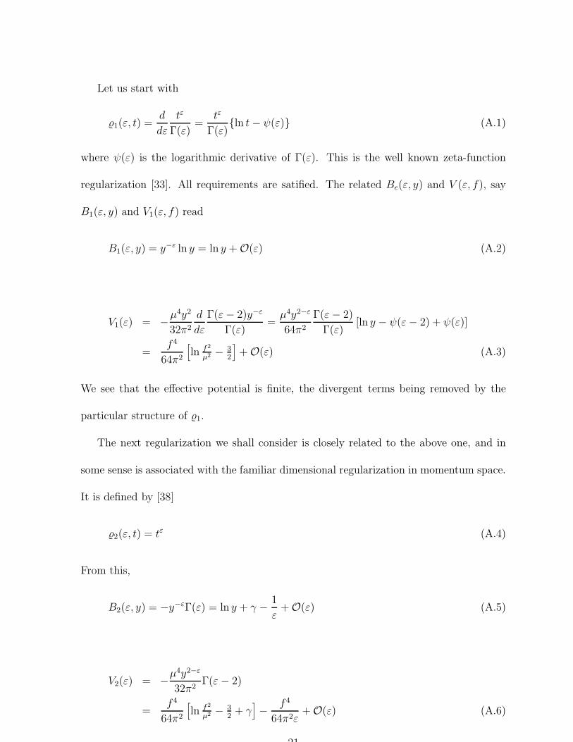
Let us start with

1(ε, t) =d

dε

tε

Γ(ε)=

tε

Γ(ε){ln t− ψ(ε)} (A.1)

where ψ(ε) is the logarithmic derivative of Γ(ε). This is the well known zeta-function

regularization [33]. All requirements are satified. The related Be(ε, y) and V (ε, f), say

B1(ε, y) and V1(ε, f) read

B1(ε, y) = y−ε ln y = ln y + O(ε) (A.2)

V1(ε) = −µ4y2

32π2

d

dε

Γ(ε− 2)y−ε

Γ(ε)=µ4y2−ε

64π2

Γ(ε− 2)

Γ(ε)[ln y − ψ(ε− 2) + ψ(ε)]

=f 4

64π2

[

ln f2

µ2 − 32

]

+ O(ε) (A.3)

We see that the effective potential is finite, the divergent terms being removed by the

particular structure of 1.

The next regularization we shall consider is closely related to the above one, and in

some sense is associated with the familiar dimensional regularization in momentum space.

It is defined by [38]

2(ε, t) = tε (A.4)

From this,

B2(ε, y) = −y−εΓ(ε) = ln y + γ − 1

ε+ O(ε) (A.5)

V2(ε) = −µ4y2−ε

32π2Γ(ε− 2)

=f 4

64π2

[

ln f2

µ2 − 32

+ γ]

− f 4

64π2ε+ O(ε) (A.6)

21

easily follow, again in agreement with the general result. Within this regularization, only

one divergent term is present.

Another often used regularization is the ultraviolet cut-off regularization, defined by

3(ε, t) = θ(t− ε) (A.7)

In this case we have

B3(ε, y) = −Γ(0, yε) = ln y + γ + ln ε+ O(ε) (A.8)

V3(ε) = −µ4y2Γ(−2, εy)

32π2

=f 4

64π2

[

ln f2

µ2 − 32

+ γ]

− µ4

64π2ε2+

µ2f 2

32π2ε+

f 4

64π2ln ε+ O(ε) (A.9)

Here we have three divergent terms. From these examples, it is obvious that they depend

on the regularization function.

The fourth regularization reads

4(ε, t) = e−ε/4t (A.10)

We have

B4(ε, y) = −2K0(√εy) = ln y + 2γ − 2 ln 2 + ln ε+ O(ε) (A.11)

V4(ε) = − µ4y

4επ2K2(

√εy)

=f 4

64π2

[

ln f2

µ2 − 32

+ 2γ − 2 ln 2]

− µ4

2π2ε2+µ2f 2

8π2ε+

f 4

64π2ln ε+ O(ε) (A.12)

Kν being the Mc Donald functions.

22

The last regularization we would like to consider is presented as an example of the

freedom one has. It is similar to a Pauli-Villars type and it is defined by (α being an

arbitrary positive constant)

5(ε, t) = (1 − e−αt/ε)3 (A.13)

the power 3 being related to the fact that we are working in four dimensions. This is a

general feature of the Pauli-Villars regularization. We have

B5(ε, y) = ln εyεy+3α

+ 3 ln εy+2αεy+α

= ln y + ln 83α

+ ln ε+ O(ε) (A.14)

V5(ε) =µ4y2

64π2

{

[

ln εyα− 3

2

]

− 3(

1 + αεy

)2 [

ln(

1 + εyα

)

− 32

]

+ 3(

1 + 2αεy

)2 [

ln(

2 + εyα

)

− 32

]

−(

1 + 3αεy

)2 [

ln(

3 + εyα

)

− 32

]

}

=f 4

64π2

[

ln f2

µ2 − 32

+ ln 8α3

]

+3α2 ln(16/27)µ4

64π2ε2(A.15)

+3α ln(16/9)µ2f 2

64π2ε+

f 4

64π2ln ε+ O(ε)

With this example we conclude the list of possible regularization functions.

B Appendix: heat kernel expansion and zeta-function

For convenience of the reader, here we just report on some results concerning heat kernel

expansion and zeta function. To start with we consider a second order elliptic differential

operator A = −△ + X(x) defined on a smooth D-dimensional Riemannian manifold

without boundary (X(x) is a scalar function). The results we are going to discuss have

been quite recently given also for Riemannian manifolds with boundary [39, 40, 41, 42]

23

and also in the presence of torsion [43, 44]. The kernel of the operator exp(−tA), which

satisfies a heat type equation, has an asymptotic expansion, valid for small t, given by

Kt(x, x;A) ∼ 1

(4πt)N/2

∞∑

n=0

an(x;A)tn (B.1)

an(x;A) being the spectral (Minakshisundaram, Seeley, DeWitt, Gilkey) coefficients,

which are invariant quantities built up with curvature and their derivatives. Some of

such coefficients are computed by many authors (see for example refs. [39]). In particular

we have (of course a0(x;A) = 1)

a1(x;A) =R

6−X (B.2)

a2(x;A) = 12a2

1 + 16△a1 + 1

180

[

△R +RijrsRijrs − RijRij

]

(B.3)

Sometimes it may be convenient to factorize the exponential exp(ta1) and consider an

expansion very closely related to eq. (B.1), that is [45]

Kt(x, x;A) ∼ e−t(X−R/6)

(4πt)N/2

∞∑

n=0

bn(x;A)tn (B.4)

with b0 = 1, b1 = 0 and more generally

an(x;A) =n∑

l=0

bn−lal1

l!(B.5)

bn(x;A) =n∑

l=0

(−1)lan−lal1

l!(B.6)

In this way, all coefficients bn do not depend on a1 [45].

The connection between heat kernel and zeta-function is realized by means of the

Mellin representation

ζ(s;A) =1

Γ(s)

∫ ∞

0ts−1 Tr e−tAdt (B.7)

24

Using expansion (B.1) in this latter expression, we can get the meromorphic structure of

ζ(s;A) as given by Seeley in ref. [46]. If we suppose −a1 to be a positive function, say a2,

we can obtain the zeta-function as a power series of the kind

ζ(s;A/µ2) ∼∑

n≥0

µ2sΓ(s+ n−D/2)

(4π)D/2Γ(s)

∫

Mbna

−2(s+n−D/2) √g dDx (B.8)

from which eq. (5.6) follows and for D = 4 one obtains furthermore

ζ ′(0;A/µ2) ∼ 1

16π2

∫

M

34a4 − a2 ln a2

µ2 +∑

n≥1

(n− 1)!bn+2

a2n

√g d4x (B.9)

concluding the summary of useful results.

References

[1] N.D. Birrell and P.C.W. Davies. Quantum fields on curved space. Cambridge Uni-

versity Press, Cambridge, England, (1982).

[2] R.H. Brandenberger. Rev. Mod. Phys., 57, 1, (1985).

[3] R. Jackiw. Phys. Rev. D, 9, 1686, (1974).

[4] D.J. Toms. Phys. Rev., 26, 2713, (1982).

[5] L.Ford and T. Yoshimura. Phys. Lett. A, 70, 89, (1979).

[6] L.Ford . Phys. Rev. D, 21, 933, (1980).

[7] D.J. Toms. Phys. Rev. D, 21, 2805, (1980).

[8] D.J. Toms. Ann. Phys., 129, 334, (1980).

[9] G. Denardo and E. Spallucci. Nuovo Cimento A, 58, 243, (1980).

25

[10] G. Denardo and E. Spallucci. Nucl. Phys. B, 169, 514, (1980).

[11] G. Kennedy. Phys. Rev. D, 23, 2884, (1981).

[12] A. Actor. Class. Quantum Grav., 7, 1463, (1990).

[13] E. Elizalde and A. Romeo. Phys. Lett. B, 244, 387, (1990).

[14] P. Chang and J.S. Dowker. Vacuum energy on orbifold factors of spheres. Technical

Report, Preprint, Manchester University, (1992).

[15] G.F.R. Ellis. Gen. Rel. Grav., 2, 7, (1971).

[16] W.P. Thurston. Bull. Amer. Math. Soc., 6, 357, (1982).

[17] R.D. Ball. Phys. Rep., 182, 1, (1989).

[18] S. Coleman and E. Weinberg. Phys. Rev., 7, 1888, (1973).

[19] J. Iliopoulos, C. Itzykson and A. Martin. Rev. Mod. Phys., 47, 165, (1975).

[20] J. Elstrodt, F. Grunewald and J. Mennicke. Math. Ann., 277, 655, (1987).

[21] A. Selberg. J. Indian Math Soc., 20, 47, (1956).

[22] I. Chavel. Eigenvalues in Riemannian geometry. Academic Press, Inc. U.S.A., (1984).

[23] D.J. Toms. Phys. Rev. D, 21, 928, (1979).

[24] N.D. Birrell and L. Ford. Phys. Rev. D, 22, 330, (1980).

[25] B.S. Kay. Phys. Rev. D, 20, 3052, (1979).

[26] I.S. Gradshteyn and I.M Ryzhik. Table of integrals, series and products. Academic

press, Inc., New York, (1980).

26

[27] A.A. Bytsenko and S. Zerbini. Class. Quantum Grav., 9, 1365, (1992).

[28] R. Utiyama and B. DeWitt. J. Math. Phys., 3, 608, (1962).

[29] B.L. Hu and D.J. O’Connors . Phys. Rev., 30, 743, (1984).

[30] A.L. Berkin. Phys. Rev., 46, 1551, (1992).

[31] B.L. Nelson and P. Panangaden. Phys. Rev., 25, 1019, (1982).

[32] I.L. Buchbinder, S.D. Odintsov and I.L. Shapiro. Effective Action in Quantum Grav-

ity. A. Hilger, Bristol, (1992).

[33] S.W. Hawking. Comm. Math. Phys., 55, 133, (1977).

[34] B.S. DeWitt. The dynamical theory of groups and fields. Gordon and Breach, New

York, (1965).

[35] P.B. Gilkey. J. Diff. Geometry, 10, 601, (1975).

[36] D.J. O’Connors, B.L. Hu and T.C. Shen . Phys. Lett. B, 130, 31, (1983).

[37] A.B. Venkov. Russian Math. Surveys, 34, 79, (1979).

[38] J.S. Dowker and R. Critchley. Phys. Rev. D, 13, 3224, (1976).

[39] T.P. Branson and P.B.Gilkey. Comm. Part. Diff. Eqs., 15, 245, (1990).

[40] G. Cognola, L. Vanzo and S. Zerbini. Phys. Lett. B, 241, 381, (1990).

[41] D.M. McAvity and H. Osborn. Class. Quantum Grav., 8, 603, (1991).

[42] A. Dettki and A. Wipf. Nucl. Phys. B, 377, 252, (1992).

[43] Yu.N. Obukhov. Phys. Lett. B, 108, 308, (1982).

27

[44] G. Cognola and S. Zerbini. Phys. Lett. B, 214, 70, (1988).

[45] I. Jack and L. Parker. Phys. Rev. D, 31, 2439, (1985).

[46] R.T. Seeley. Am. Math. Soc. Prog. Pure Math., 10, 172, (1967).

28