Ondulo Defects Detection Software - Rhopoint Instruments Defects Detection... · Ondulo Defects Detection Software Instruction Manual Ver: 1.0.30.8167 Thank you for purchasing this

Ondulo Defects Detection Software

Instruction Manual

Ver: 1.0.30.8167

Thank you for purchasing this Rhopoint product. Please read these instructions carefully before use and retain for future reference. The images shown in this manual are for illustrative purposes only.

English

2

This instruction manual contains important information about the setup and use of Ondulo Defects Detection Software. It is therefore essential that the contents be read before using the software. If the software is to be used by others you must ensure that this instruction manual and license dongle is supplied with the software. If you have any questions or require additional information about Ondulo Defects Detection please contact the Rhopoint Authorised Distributor for your region. As part of Rhopoint Instruments commitment to continually improving the software used with their products, they reserve the right to change the information included in this document without prior notice. © Copyright 2014 Rhopoint Instruments Ltd. All Rights Reserved. Ondulo and Rhopoint are registered trademarks or trademarks of Rhopoint Instruments Ltd. in the UK and other countries. Other product and company names mentioned herein may be trademarks of their respective owner. No portion of the software, documentation or other accompanying materials may be

translated, modified, reproduced, copied or otherwise duplicated ( with the exception

of a backup copy), or distributed to a third party, without prior written authorization

from Rhopoint Instruments Ltd.

Rhopoint Instruments Ltd. Enviro 21 Business Park Queensway Avenue South St Leonards on Sea TN38 9AG UK Tel: +44 (0)1424 739622 Fax: +44 (0)1424 730600 Email: [email protected] Website: www.rhopointinstruments.com Revision A May 2015

3

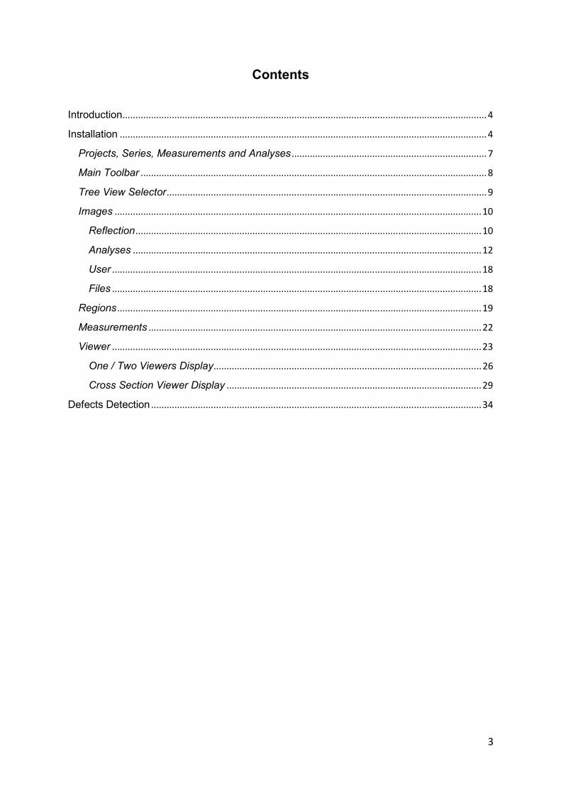
Contents

Introduction ............................................................................................................................................ 4

Installation ............................................................................................................................................. 4

Projects, Series, Measurements and Analyses ........................................................................... 7

Main Toolbar ..................................................................................................................................... 8

Tree View Selector ........................................................................................................................... 9

Images ............................................................................................................................................. 10

Reflection ..................................................................................................................................... 10

Analyses ...................................................................................................................................... 12

User .............................................................................................................................................. 18

Files .............................................................................................................................................. 18

Regions ............................................................................................................................................ 19

Measurements ................................................................................................................................ 22

Viewer .............................................................................................................................................. 23

One / Two Viewers Display ....................................................................................................... 26

Cross Section Viewer Display .................................................................................................. 29

Defects Detection ............................................................................................................................... 34

4

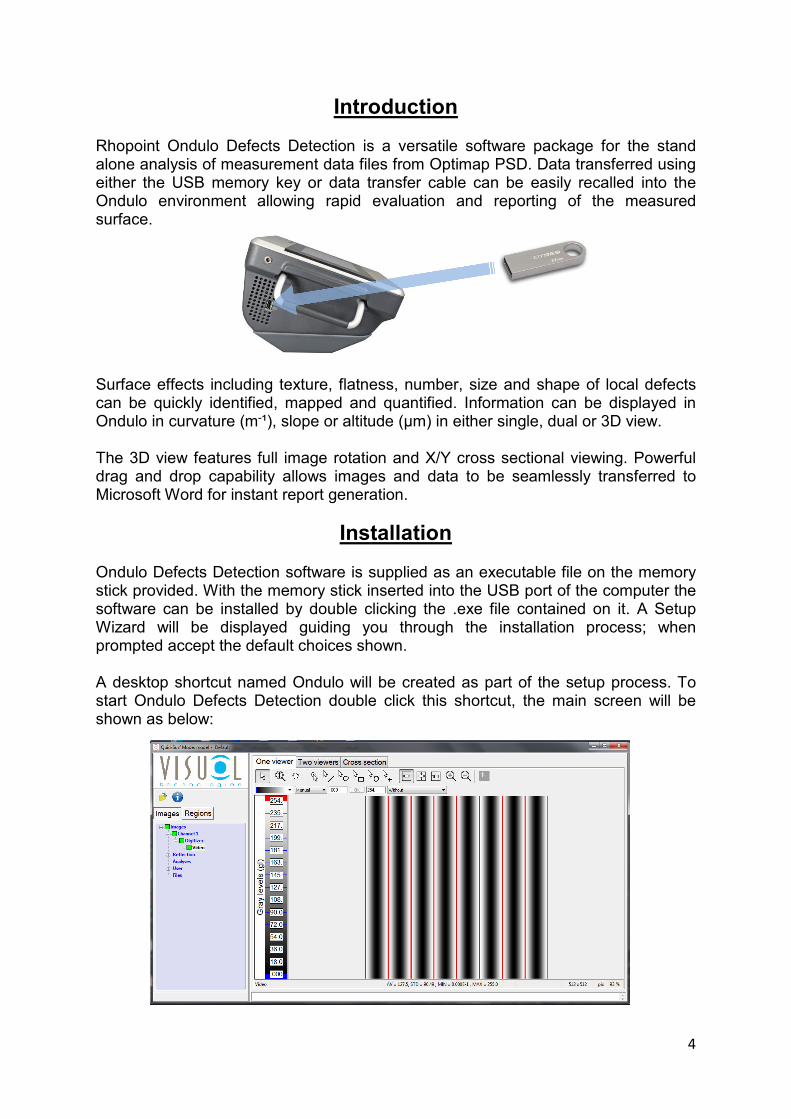
Introduction

Rhopoint Ondulo Defects Detection is a versatile software package for the stand alone analysis of measurement data files from Optimap PSD. Data transferred using either the USB memory key or data transfer cable can be easily recalled into the Ondulo environment allowing rapid evaluation and reporting of the measured surface. Surface effects including texture, flatness, number, size and shape of local defects can be quickly identified, mapped and quantified. Information can be displayed in Ondulo in curvature (m-¹), slope or altitude (μm) in either single, dual or 3D view. The 3D view features full image rotation and X/Y cross sectional viewing. Powerful drag and drop capability allows images and data to be seamlessly transferred to Microsoft Word for instant report generation.

Installation

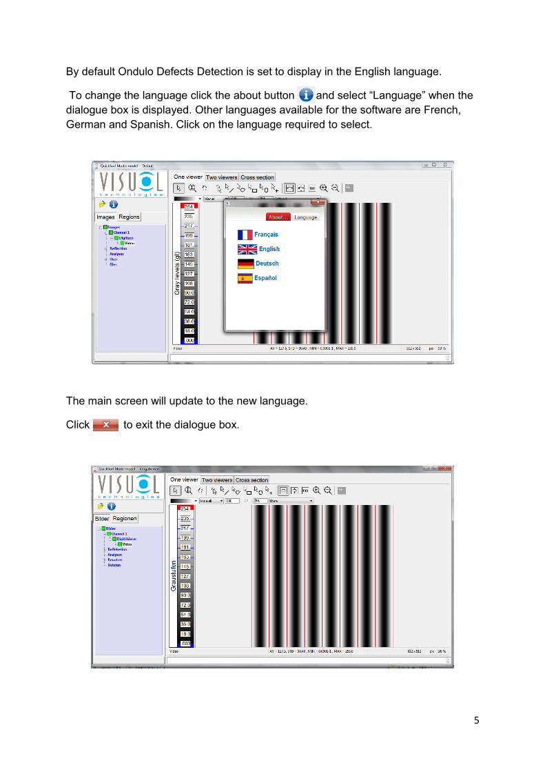
Ondulo Defects Detection software is supplied as an executable file on the memory stick provided. With the memory stick inserted into the USB port of the computer the software can be installed by double clicking the .exe file contained on it. A Setup Wizard will be displayed guiding you through the installation process; when prompted accept the default choices shown. A desktop shortcut named Ondulo will be created as part of the setup process. To start Ondulo Defects Detection double click this shortcut, the main screen will be shown as below:

5

By default Ondulo Defects Detection is set to display in the English language.

To change the language click the about button and select “Language” when the

dialogue box is displayed. Other languages available for the software are French,

German and Spanish. Click on the language required to select.

The main screen will update to the new language.

Click to exit the dialogue box.

6

Overview

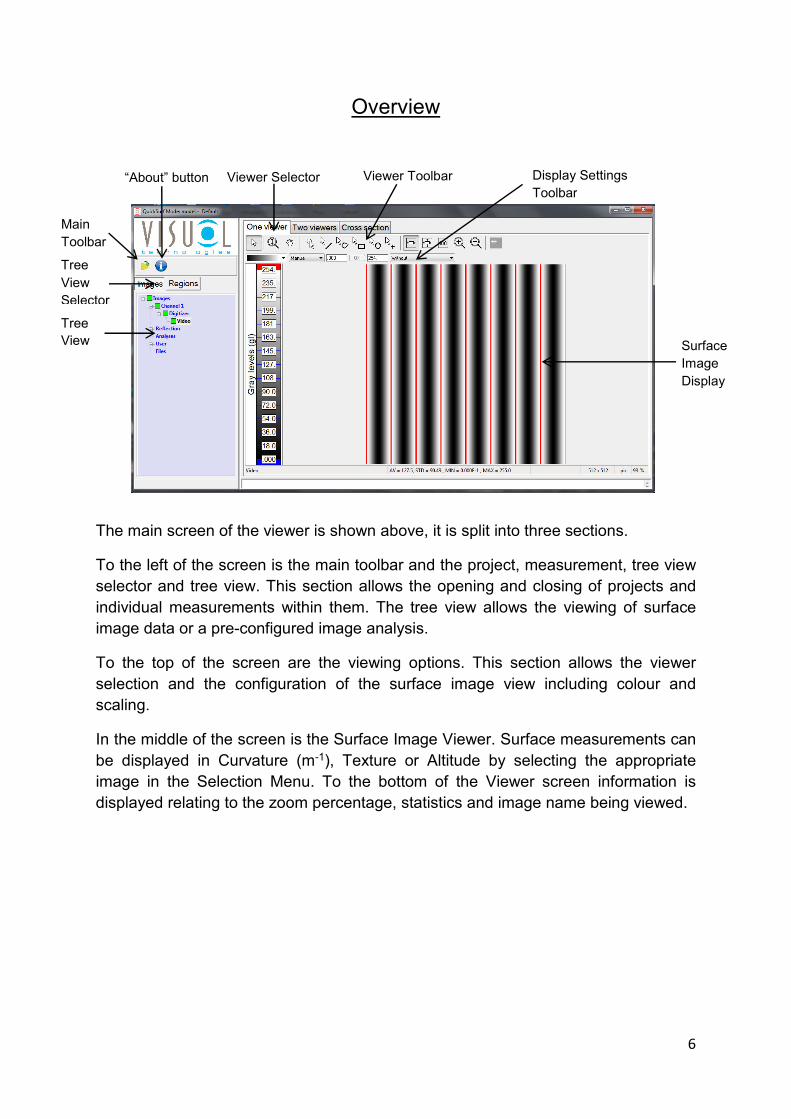
The main screen of the viewer is shown above, it is split into three sections.

To the left of the screen is the main toolbar and the project, measurement, tree view

selector and tree view. This section allows the opening and closing of projects and

individual measurements within them. The tree view allows the viewing of surface

image data or a pre-configured image analysis.

To the top of the screen are the viewing options. This section allows the viewer

selection and the configuration of the surface image view including colour and

scaling.

In the middle of the screen is the Surface Image Viewer. Surface measurements can

be displayed in Curvature (m-1), Texture or Altitude by selecting the appropriate

image in the Selection Menu. To the bottom of the Viewer screen information is

displayed relating to the zoom percentage, statistics and image name being viewed.

Viewer Selector Viewer Toolbar Display Settings

Toolbar

Main

Toolbar

Tree

View Surface

Image

Display

Tree

View

Selector

“About” button

7

Projects, Series, Measurements and Analyses

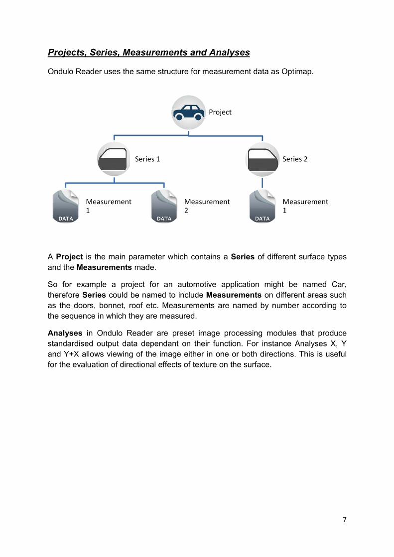
Ondulo Reader uses the same structure for measurement data as Optimap.

A Project is the main parameter which contains a Series of different surface types

and the Measurements made.

So for example a project for an automotive application might be named Car,

therefore Series could be named to include Measurements on different areas such

as the doors, bonnet, roof etc. Measurements are named by number according to

the sequence in which they are measured.

Analyses in Ondulo Reader are preset image processing modules that produce

standardised output data dependant on their function. For instance Analyses X, Y

and Y+X allows viewing of the image either in one or both directions. This is useful

for the evaluation of directional effects of texture on the surface.

Project

Series 1

Measurement

1

Measurement

2

Series 2

Measurement

1

8

Main Toolbar

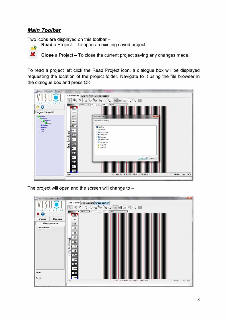
Two icons are displayed on this toolbar – Read a Project – To open an existing saved project. Close a Project – To close the current project saving any changes made.

To read a project left click the Read Project icon, a dialogue box will be displayed

requesting the location of the project folder. Navigate to it using the file browser in

the dialogue box and press OK.

The project will open and the screen will change to –

9

Tree View Selector

With a project open, three tabs are displayed -

Images – Containing image data and analyses in a tree view

Regions - This tree view enables management of regions (creation, edition and deletion) in a picture. Measurements - Selection menu tree containing individual measurements within the

project grouped according to Series

To open a measurement select the Measurements tab. Each measurement

contains the series within the project.

In the example displayed above one series is displayed, 1, containing two

measurements (01, 02).

Double clicking the measurement opens it.

10

Images

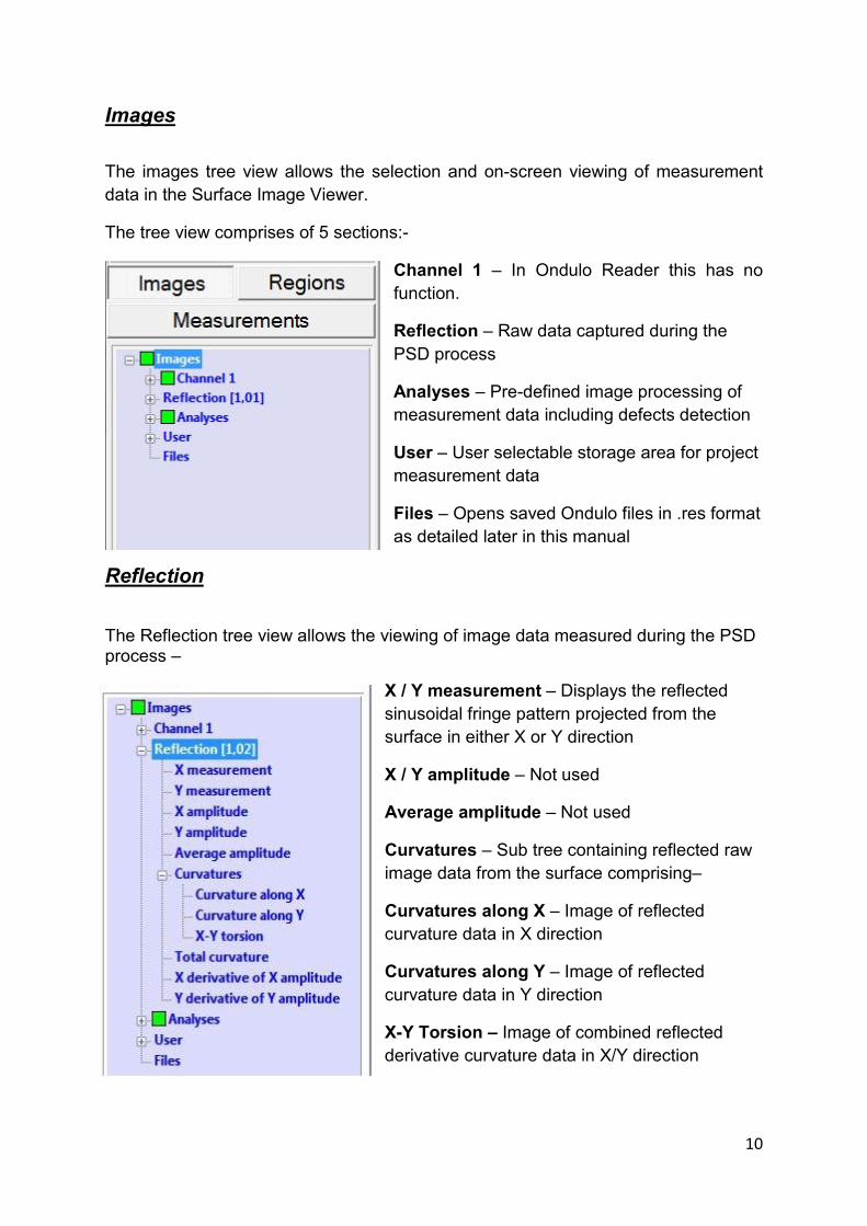
The images tree view allows the selection and on-screen viewing of measurement

data in the Surface Image Viewer.

The tree view comprises of 5 sections:-

Channel 1 – In Ondulo Reader this has no

function.

Reflection – Raw data captured during the

PSD process

Analyses – Pre-defined image processing of

measurement data including defects detection

User – User selectable storage area for project

measurement data

Files – Opens saved Ondulo files in .res format

as detailed later in this manual

Reflection

The Reflection tree view allows the viewing of image data measured during the PSD process –

X / Y measurement – Displays the reflected

sinusoidal fringe pattern projected from the

surface in either X or Y direction

X / Y amplitude – Not used

Average amplitude – Not used

Curvatures – Sub tree containing reflected raw

image data from the surface comprising–

Curvatures along X – Image of reflected

curvature data in X direction

Curvatures along Y – Image of reflected

curvature data in Y direction

X-Y Torsion – Image of combined reflected

derivative curvature data in X/Y direction

11

Total Curvature – Image of total curvature data

X derivative of X amplitude – Not used

Y derivative of Y amplitude – Not used

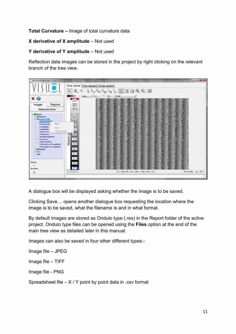
Reflection data images can be stored in the project by right clicking on the relevant

branch of the tree view.

A dialogue box will be displayed asking whether the image is to be saved.

Clicking Save… opens another dialogue box requesting the location where the

image is to be saved, what the filename is and in what format.

By default images are stored as Ondulo type (.res) in the Report folder of the active

project. Ondulo type files can be opened using the Files option at the end of the

main tree view as detailed later in this manual.

Images can also be saved in four other different types:-

Image file – JPEG

Image file – TIFF

Image file - PNG

Spreadsheet file – X / Y point by point data in .csv format

12

Analyses

The Analyses tree allows the viewing of processed measurement data.

Ondulo Defects Detection software contains preset analyses that produce

standardised output images and also user configurable defects detection on any of

the analysed images.

When a measurement is opened all analyses set to “Auto” are run automatically.

These analyses are shown in bold font. When run a green box appears to the left of

the analyses indicating that it has run successfully. Analyses which are set to

“Manual” are shown in normal font no green box is displayed.

The analyses tree contains the following labels;-

X – Displays surface curvature image data in X

direction

Y – Displays surface curvature image data in Y

direction

Y+X - Displays surface curvature image data in

X/Y direction

01 – Unwrap X to Altitude BF – Preset analysis

to convert curvature image data into altitude

image data in μm. Altitude BF is the analyses

containing the converted altitude image map.

X – A - Displays band filtered (0.1mm - 0.3mm)

curvature image data in X direction

X – B - Displays band filtered (0.3mm - 1mm)

curvature image data in X direction

X – C - Displays band filtered (1mm - 3mm)

curvature image data in X direction

X – D - Displays band filtered (3mm - 10mm)

curvature image data in X direction

X – E - Displays band filtered (10mm - 30mm) curvature image data in X direction

X – L - Displays band filtered (0.3mm -1.2mm) curvature image data in X direction

X – S - Displays band filtered (1.2mm - 12mm) curvature image data in X direction

Y – A - Displays band filtered (0.1mm – 0.3mm) curvature image data in Y direction

13

Y – B - Displays band filtered (0.3mm - 1mm) curvature image data in Y direction

Y – C - Displays band filtered (1mm - 3mm) curvature image data in Y direction

Y – D - Displays band filtered (3mm - 10mm) curvature image data in Y direction

Y – E - Displays band filtered (10mm - 30mm) curvature image data in Y direction

Y – L - Displays band filtered (0.3mm -1.2mm) curvature image data in Y direction

Y – S - Displays band filtered (1.2mm - 12mm) curvature image data in Y direction

Y – A - Displays band filtered (0.1mm – 0.3mm) curvature image data in Y direction

Y – B - Displays band filtered (0.3mm - 1mm) curvature image data in Y direction

Y – C - Displays band filtered (1mm - 3mm) curvature image data in Y direction

Y – D - Displays band filtered (3mm - 10mm) curvature image data in Y direction

Y – E - Displays band filtered (10mm - 30mm) curvature image data in Y direction

Y – L - Displays band filtered (0.3mm -1.2mm) curvature image data in Y direction

Y – S - Displays band filtered (1.2mm - 12mm) curvature image data in Y direction

Y+X – A - Displays band filtered (0.1mm – 0.3mm) curvature image data in X/Y

direction

Y+X – B - Displays band filtered (0.3mm - 1mm) curvature image data in X/Y

direction

Y+X – C - Displays band filtered (1mm - 3mm) curvature image data in X/Y direction

Y+X – D - Displays band filtered (3mm - 10mm) curvature image data in X/Y

direction

Y+X – E - Displays band filtered (10mm - 30mm) curvature image data in X/Y

direction

Y+X – L - Displays band filtered (0.3mm -1.2mm) curvature image data in X/Y

direction

Y+X – S - Displays band filtered (1.2mm - 12mm) curvature image data in X/Y

direction

14

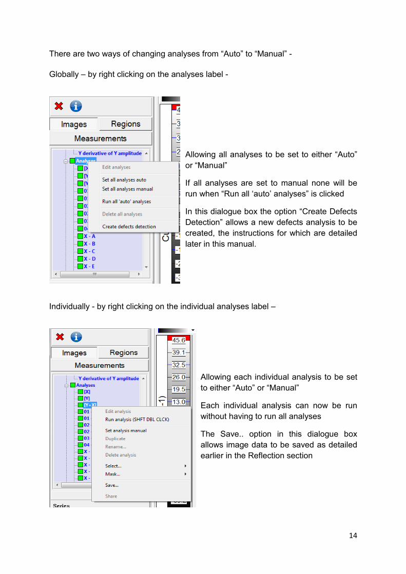
There are two ways of changing analyses from “Auto” to “Manual” -

Globally – by right clicking on the analyses label -

Allowing all analyses to be set to either “Auto”

or “Manual”

If all analyses are set to manual none will be

run when “Run all ‘auto’ analyses” is clicked

In this dialogue box the option “Create Defects

Detection” allows a new defects analysis to be

created, the instructions for which are detailed

later in this manual.

Individually - by right clicking on the individual analyses label –

Allowing each individual analysis to be set

to either “Auto” or “Manual”

Each individual analysis can now be run

without having to run all analyses

The Save.. option in this dialogue box

allows image data to be saved as detailed

earlier in the Reflection section

15

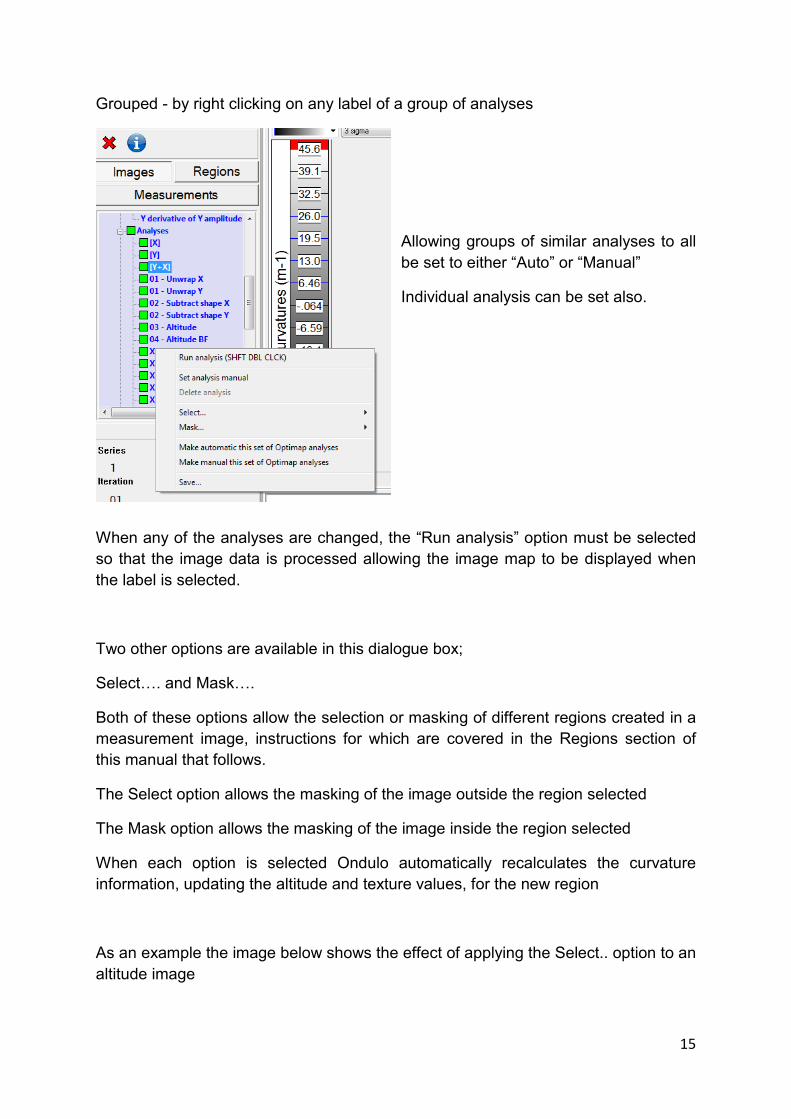
Grouped - by right clicking on any label of a group of analyses

Allowing groups of similar analyses to all

be set to either “Auto” or “Manual”

Individual analysis can be set also.

When any of the analyses are changed, the “Run analysis” option must be selected

so that the image data is processed allowing the image map to be displayed when

the label is selected.

Two other options are available in this dialogue box;

Select…. and Mask….

Both of these options allow the selection or masking of different regions created in a

measurement image, instructions for which are covered in the Regions section of

this manual that follows.

The Select option allows the masking of the image outside the region selected

The Mask option allows the masking of the image inside the region selected

When each option is selected Ondulo automatically recalculates the curvature

information, updating the altitude and texture values, for the new region

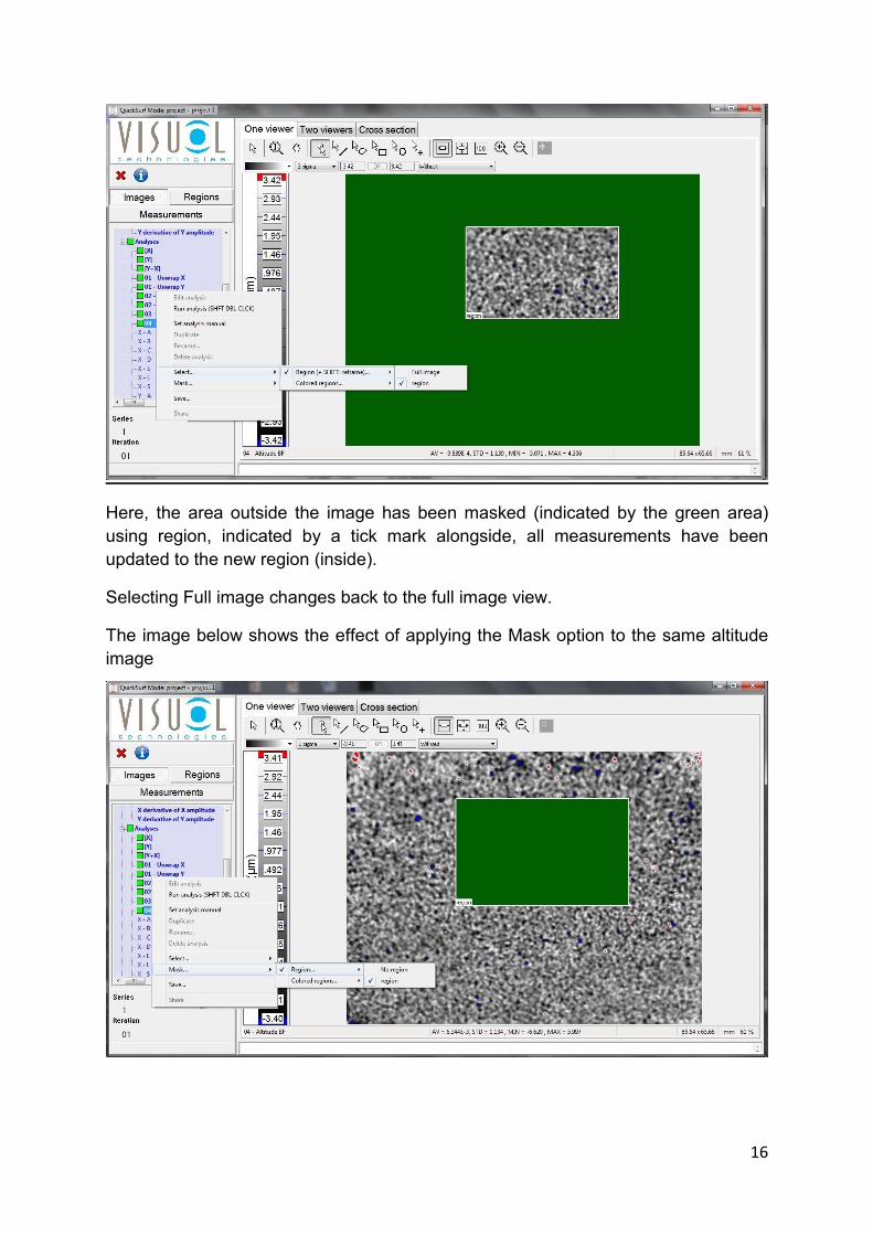
As an example the image below shows the effect of applying the Select.. option to an

altitude image

16

Here, the area outside the image has been masked (indicated by the green area)

using region, indicated by a tick mark alongside, all measurements have been

updated to the new region (inside).

Selecting Full image changes back to the full image view.

The image below shows the effect of applying the Mask option to the same altitude

image

17

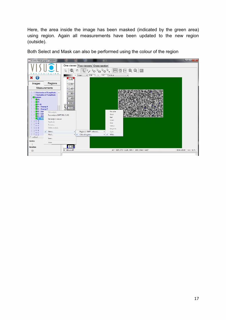
Here, the area inside the image has been masked (indicated by the green area)

using region. Again all measurements have been updated to the new region

(outside).

Both Select and Mask can also be performed using the colour of the region

18

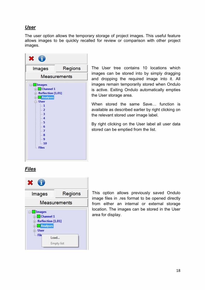
User

The user option allows the temporary storage of project images. This useful feature allows images to be quickly recalled for review or comparison with other project images.

The User tree contains 10 locations which

images can be stored into by simply dragging

and dropping the required image into it. All

images remain temporarily stored when Ondulo

is active. Exiting Ondulo automatically empties

the User storage area.

When stored the same Save… function is

available as described earlier by right clicking on

the relevant stored user image label.

By right clicking on the User label all user data

stored can be emptied from the list.

Files

This option allows previously saved Ondulo

image files in .res format to be opened directly

from either an internal or external storage

location. The images can be stored in the User

area for display.

19

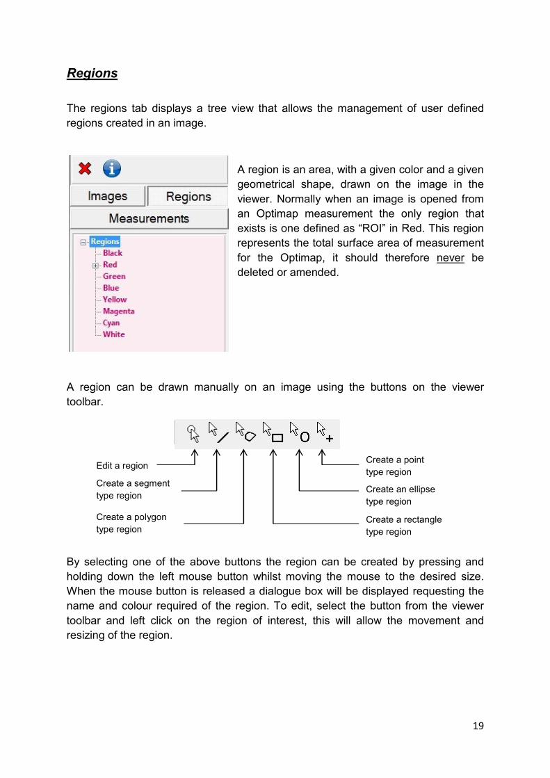
Regions

The regions tab displays a tree view that allows the management of user defined

regions created in an image.

A region is an area, with a given color and a given

geometrical shape, drawn on the image in the

viewer. Normally when an image is opened from

an Optimap measurement the only region that

exists is one defined as “ROI” in Red. This region

represents the total surface area of measurement

for the Optimap, it should therefore never be

deleted or amended.

A region can be drawn manually on an image using the buttons on the viewer

toolbar.

By selecting one of the above buttons the region can be created by pressing and

holding down the left mouse button whilst moving the mouse to the desired size.

When the mouse button is released a dialogue box will be displayed requesting the

name and colour required of the region. To edit, select the button from the viewer

toolbar and left click on the region of interest, this will allow the movement and

resizing of the region.

Edit a region

Create a segment

type region

Create a polygon

type region

Create a point

type region

Create an ellipse

type region

Create a rectangle

type region

20

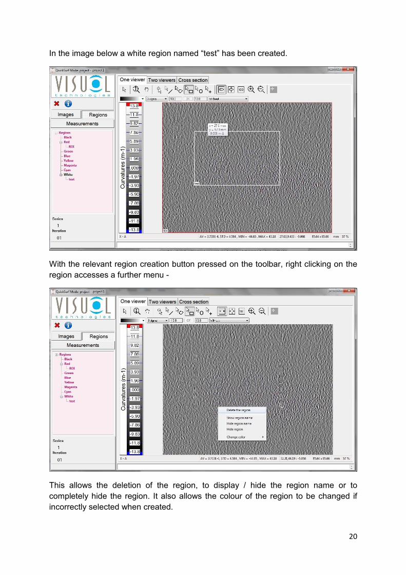
In the image below a white region named “test” has been created.

With the relevant region creation button pressed on the toolbar, right clicking on the

region accesses a further menu -

This allows the deletion of the region, to display / hide the region name or to

completely hide the region. It also allows the colour of the region to be changed if

incorrectly selected when created.

21

Right clicking on the name of a region in the tree view allows the region to be hidden,

renamed, deleted or duplicated. The region name can also be hidden.

All regions can be deleted from a colour by right clicking on the colour name

22

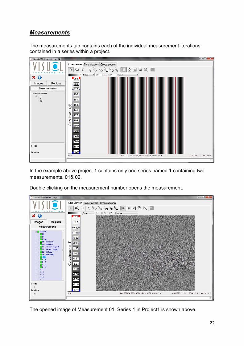
Measurements

The measurements tab contains each of the individual measurement iterations contained in a series within a project.

In the example above project 1 contains only one series named 1 containing two

measurements, 01& 02.

Double clicking on the measurement number opens the measurement.

The opened image of Measurement 01, Series 1 in Project1 is shown above.

23

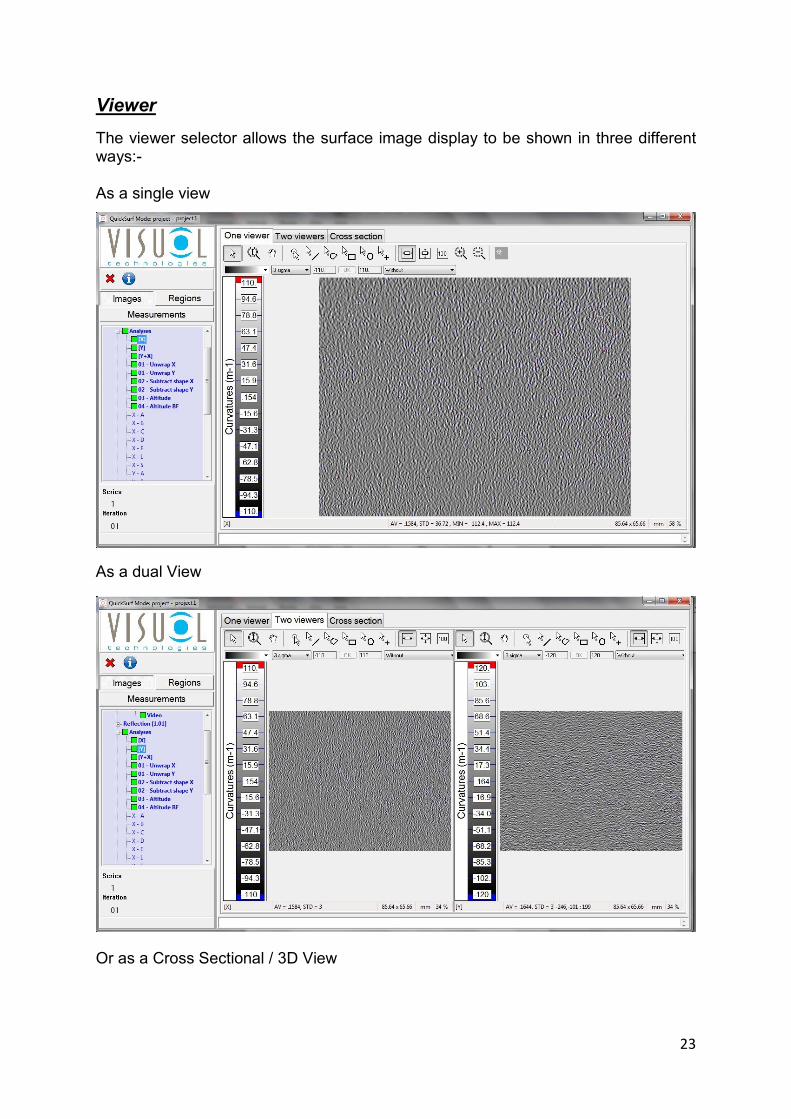
Viewer

The viewer selector allows the surface image display to be shown in three different ways:- As a single view

As a dual View

Or as a Cross Sectional / 3D View

24

The single and dual viewer displays contain the same format in terms of viewer

toolbar and colour palette. The only difference is that the dual viewer display

contains two viewing screens. This useful feature allows two images to be displayed

together allowing the analysis of each image side by side to evaluate curvature or

texture effects which are directional.

Images in both displays can be transferred (drag and drop) to Microsoft Word for

rapid reporting.

All viewer formats allow rapid full screen viewing of the image map by simply double

clicking on the image itself. In full screen mode only the image map and the viewer

toolbar are displayed allowing detailed examination of the image.

Viewer Toolbar

The viewer toolbar allows the displayed image to be adjusted according to user

requirements

Set mouse to pointer mode

Set mouse to zoom mode

25

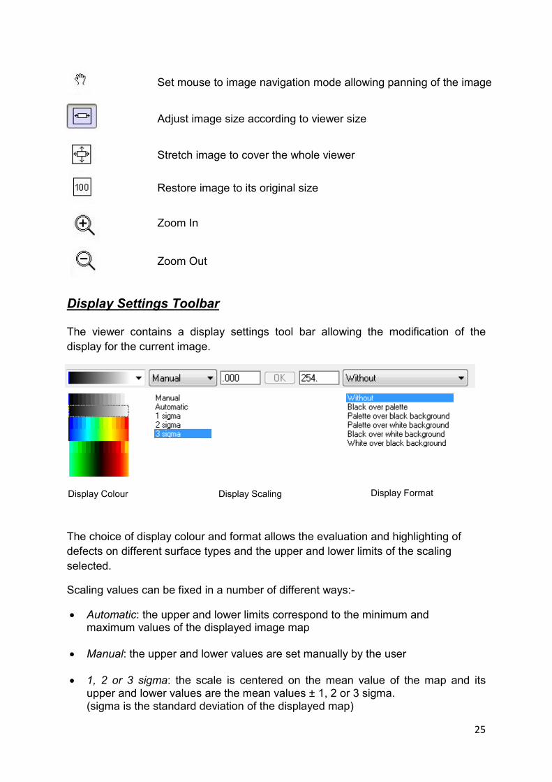
Set mouse to image navigation mode allowing panning of the image

Adjust image size according to viewer size

Stretch image to cover the whole viewer

Restore image to its original size

Zoom In

Zoom Out

Display Settings Toolbar

The viewer contains a display settings tool bar allowing the modification of the

display for the current image.

The choice of display colour and format allows the evaluation and highlighting of

defects on different surface types and the upper and lower limits of the scaling

selected.

Scaling values can be fixed in a number of different ways:-

• Automatic: the upper and lower limits correspond to the minimum and maximum values of the displayed image map

• Manual: the upper and lower values are set manually by the user

• 1, 2 or 3 sigma: the scale is centered on the mean value of the map and its upper and lower values are the mean values ± 1, 2 or 3 sigma. (sigma is the standard deviation of the displayed map)

Display Colour Display Scaling Display Format

26

One / Two Viewers Display

Right clicking on the image displays a dialogue box with the following functions-

Image name

and direction

Image stats Image

size

X, Y, Z pointer

position indicator

Zoom

level

27

Copy full image (actual scale, CTRL-C)

Actual scale copy of the full image to the clipboard, can also be actioned using Ctrl-C

Copy full image (scale = 100%, CTRL-D)

100% scale copy of the full image to the clipboard, can also be actioned using Ctrl-D

Copy image cropped by window, CTRL-E)

Copy the full image shown in the window to the clipboard, can also be actioned using

Ctrl-E

Save….

A dialogue box will be displayed asking whether the image is to be saved.

Clicking Save… opens another dialogue box requesting the location where the

image is to be saved, what the filename is and in what format.

By default images are stored as Ondulo type (.res) in the Report folder of the active

project. Ondulo type files can be opened using the Files option at the end of the

main tree view as detailed later in this manual.

Images can also be saved in four other different types:-

Image file – JPEG

Image file – TIFF

Image file - PNG

Spreadsheet file – X / Y point by point data in .csv format

Show all regions

Displays all regions available in current image

Show all regions without their names

Displays all regions available in current image without region names

Hide all regions

Hides all regions in current image

Show all regions >

Displays all coloured regions available in current image

28

Show all regions without their names >

Displays all coloured regions available in current image without region names

Hide all regions >

Hides all coloured regions in current image

Zoom >

Accesses zoom functionality

Fit in window

Stretch to window

500%

400%

300%

200%

100%

30%

10%

Tools >

Accesses viewer toolbar functions

Settings >

Allows the configuration of the viewers display -

Display hovered point information - Show / hide on screen pointer information

Scrollbars - When in zoom mode show / hide scrollbars

Rulers - Show / hide rulers

Status bar – Show / hide lower status bar

Toolbar – Show / hide viewer toolbar

Display settings toolbar - Show / hide display settings toolbar

Indicators panel - Show / hide indicators panel (not used)

Defects panel - Show / hide defects panel (not used)

29

Scale - Show / hide left hand scale

Choose this point as origin >

Set current pointer position as origin i.e. X = 0, Y = 0

Reset the origin at top left corner >

Reset the origin to the top left hand corner of the displayed image

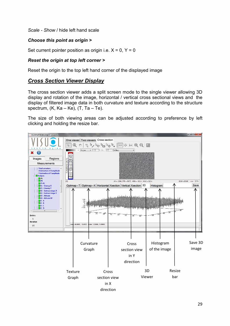
Cross Section Viewer Display

The cross section viewer adds a split screen mode to the single viewer allowing 3D display and rotation of the image, horizontal / vertical cross sectional views and the display of filtered image data in both curvature and texture according to the structure spectrum, (K, Ka – Ke), (T, Ta – Te).

The size of both viewing areas can be adjusted according to preference by left clicking and holding the resize bar.

Texture

Graph

Curvature

Graph

Cross

section view

in X

direction

Cross

section view

in Y

direction

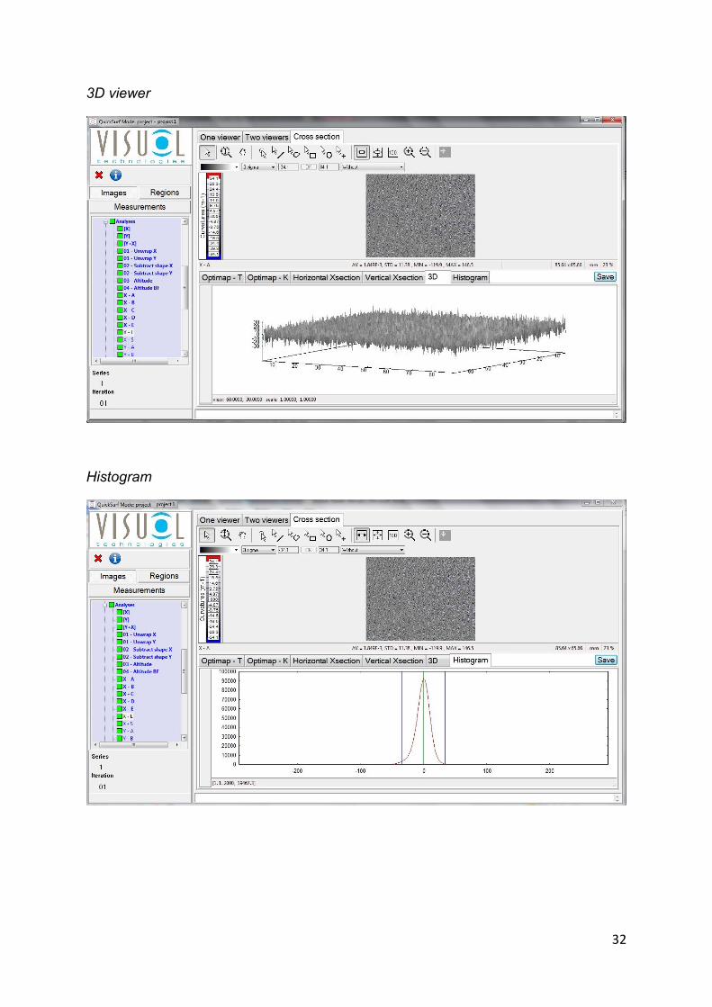
3D

Viewer

Histogram

of the image

Resize

bar

Save 3D

image

30

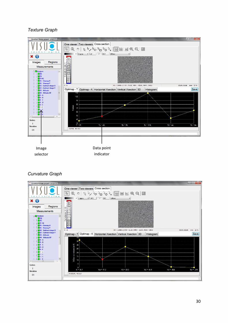
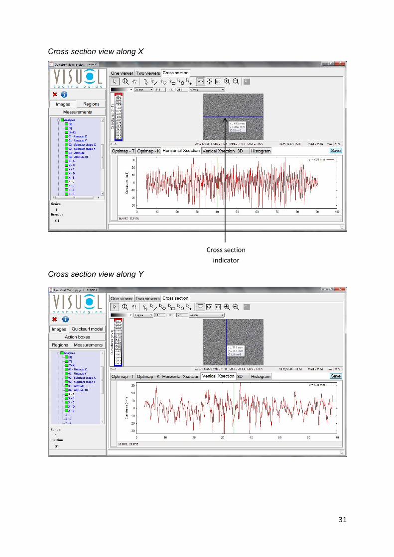
Texture Graph

Curvature Graph

Image

selector

Data point

indicator

31

Cross section view along X

Cross section view along Y

Cross section

indicator

32

3D viewer

Histogram

33

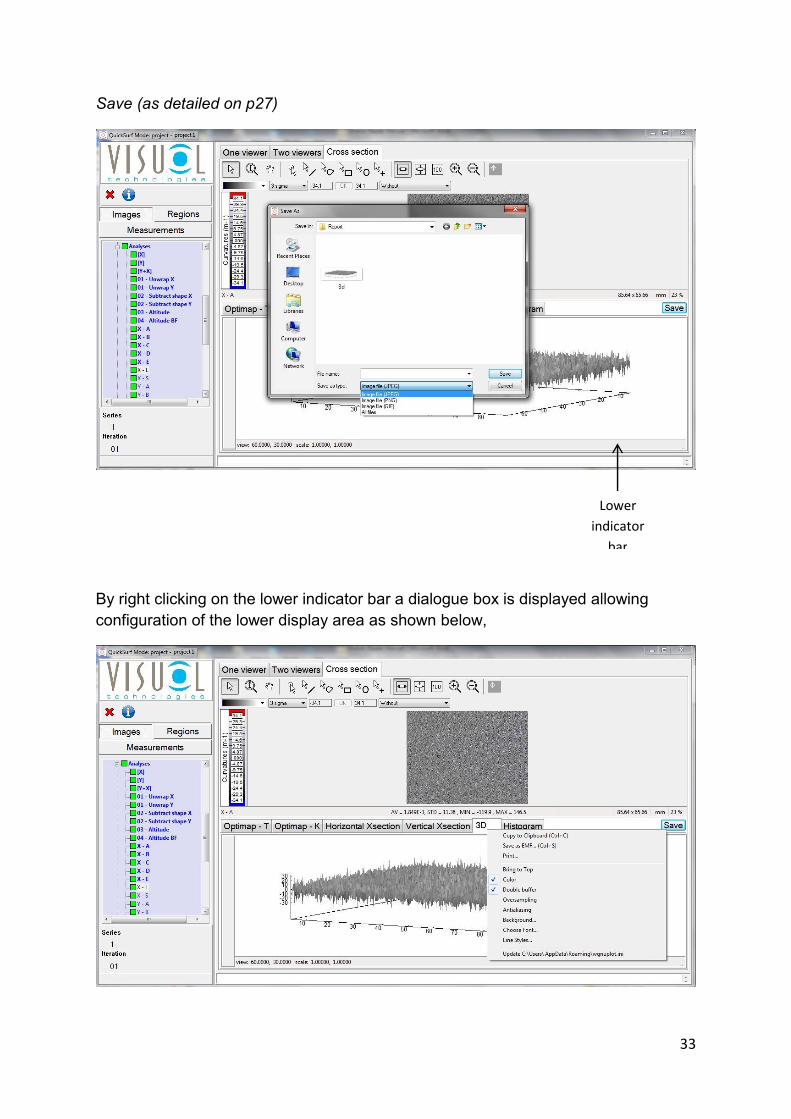
Save (as detailed on p27)

By right clicking on the lower indicator bar a dialogue box is displayed allowing

configuration of the lower display area as shown below,

Lower

indicator

bar

34

Copy to Clipboard (Ctrl+C) - Copies the 3D image displayed to the clipboard

Save as EMF … (Ctrl+S) - Save image in Enhanced Metafile format

Print …. Print the image directly to an attached printer or to pdf (if installed)

Bring to top If selected brings the image to front

Color Display in colour or black and white

Double Buffer Increases the image refresh speed

Oversampling Enable / Disable image oversampling

Antialiasing Enable / Disable image antialiasing

Background Set background colour

Choose Font Set display font

Line Styles Select line styles used

Update C:*.* Updates and save Ondulo reader settings

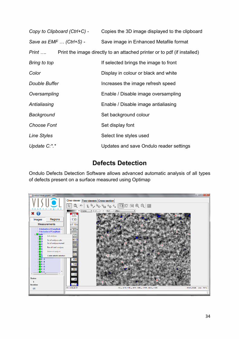
Defects Detection

Ondulo Defects Detection Software allows advanced automatic analysis of all types

of defects present on a surface measured using Optimap

35

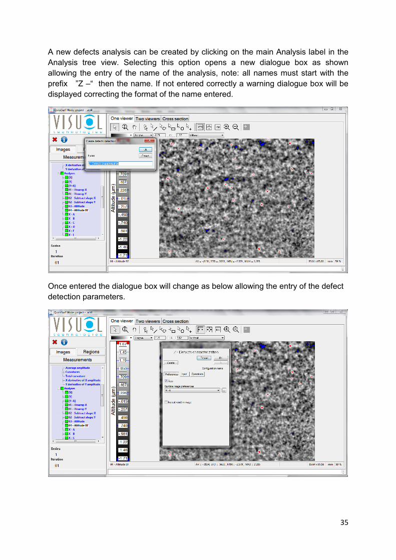
A new defects analysis can be created by clicking on the main Analysis label in the

Analysis tree view. Selecting this option opens a new dialogue box as shown

allowing the entry of the name of the analysis, note: all names must start with the

prefix ”Z –“ then the name. If not entered correctly a warning dialogue box will be

displayed correcting the format of the name entered.

Once entered the dialogue box will change as below allowing the entry of the defect

detection parameters.

36

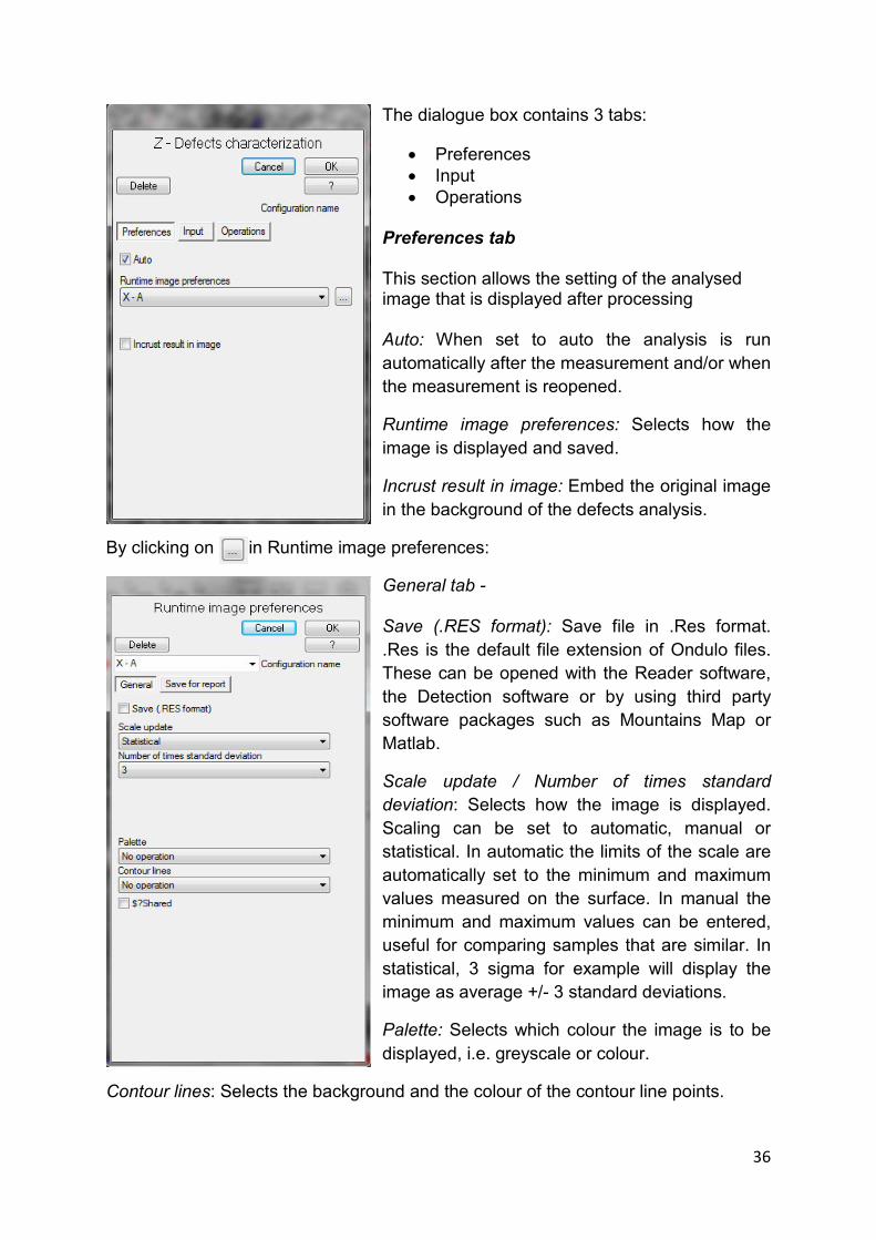
The dialogue box contains 3 tabs:

• Preferences

• Input

• Operations Preferences tab This section allows the setting of the analysed image that is displayed after processing Auto: When set to auto the analysis is run

automatically after the measurement and/or when

the measurement is reopened.

Runtime image preferences: Selects how the

image is displayed and saved.

Incrust result in image: Embed the original image

in the background of the defects analysis.

By clicking on in Runtime image preferences:

General tab - Save (.RES format): Save file in .Res format.

.Res is the default file extension of Ondulo files.

These can be opened with the Reader software,

the Detection software or by using third party

software packages such as Mountains Map or

Matlab.

Scale update / Number of times standard

deviation: Selects how the image is displayed.

Scaling can be set to automatic, manual or

statistical. In automatic the limits of the scale are

automatically set to the minimum and maximum

values measured on the surface. In manual the

minimum and maximum values can be entered,

useful for comparing samples that are similar. In

statistical, 3 sigma for example will display the

image as average +/- 3 standard deviations.

Palette: Selects which colour the image is to be

displayed, i.e. greyscale or colour.

Contour lines: Selects the background and the colour of the contour line points.

37

Save for report tab -

Report image elements: Allows the displayed image to be saved in a number of

different formats within the project (as defined on page 27). Images can be saved

individually, with or without scaling and header information, or in two separate files.

Images can also be saved with any regions that have been created (as detailed on

pages 19 – 21).

Each new configuration produced within the preferences tab should be renamed and

saved as a new user defined configuration file for future use. This way the default

configuration will not be overwritten each time.

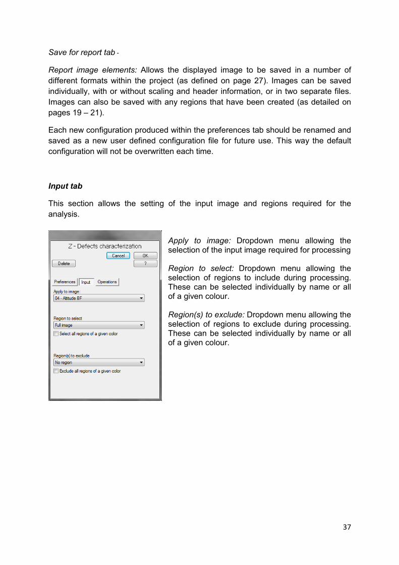
Input tab

This section allows the setting of the input image and regions required for the

analysis.

Apply to image: Dropdown menu allowing the selection of the input image required for processing Region to select: Dropdown menu allowing the selection of regions to include during processing. These can be selected individually by name or all of a given colour. Region(s) to exclude: Dropdown menu allowing the selection of regions to exclude during processing. These can be selected individually by name or all of a given colour.

38

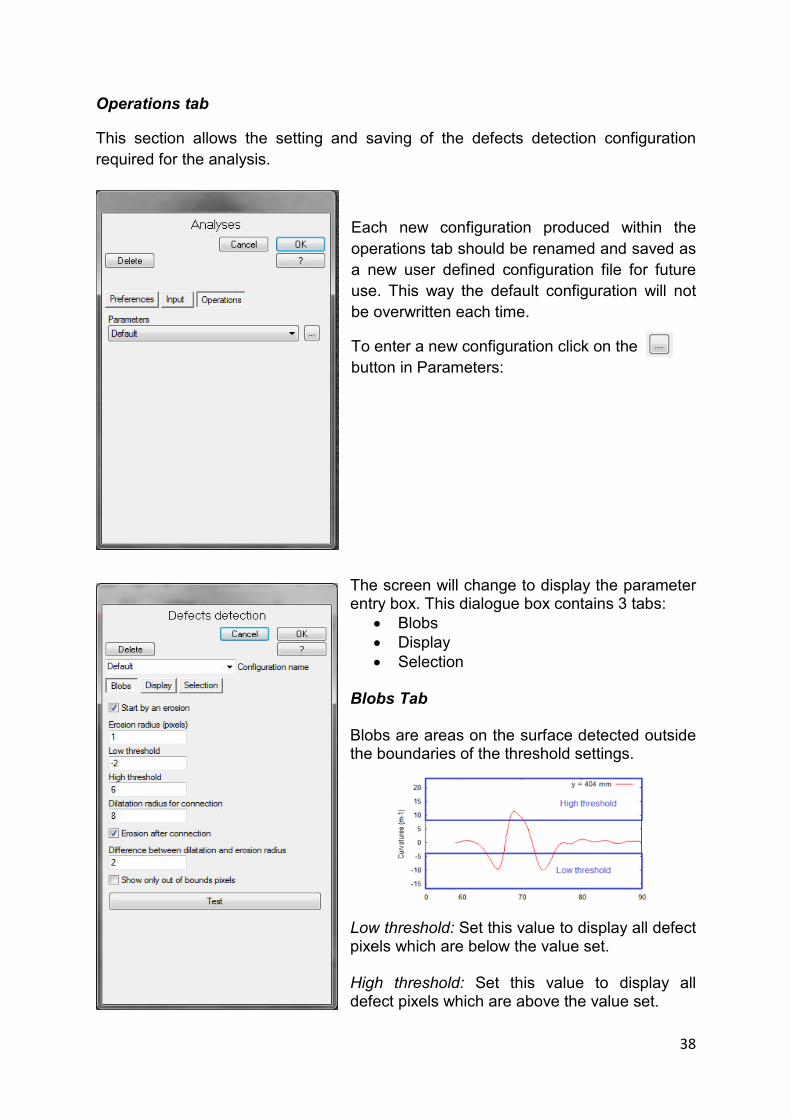
Operations tab

This section allows the setting and saving of the defects detection configuration

required for the analysis.

Each new configuration produced within the

operations tab should be renamed and saved as

a new user defined configuration file for future

use. This way the default configuration will not

be overwritten each time.

To enter a new configuration click on the

button in Parameters:

The screen will change to display the parameter entry box. This dialogue box contains 3 tabs:

• Blobs

• Display

• Selection Blobs Tab Blobs are areas on the surface detected outside the boundaries of the threshold settings.

Low threshold: Set this value to display all defect pixels which are below the value set. High threshold: Set this value to display all defect pixels which are above the value set.

39

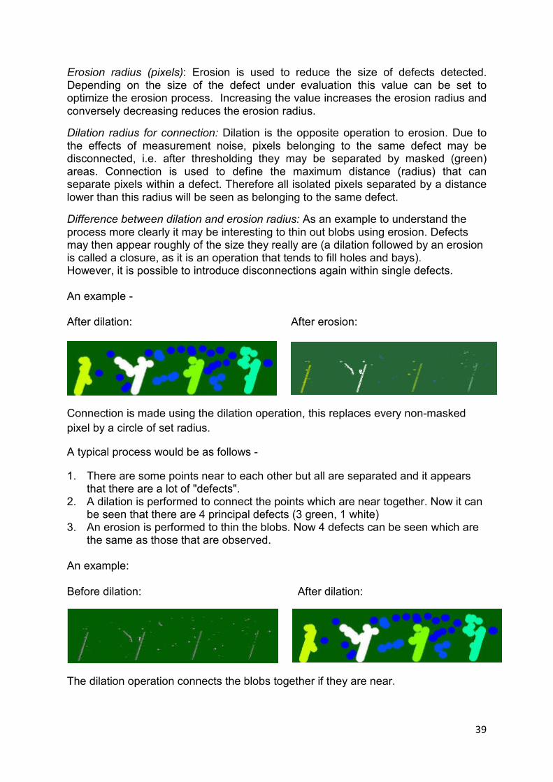
Erosion radius (pixels): Erosion is used to reduce the size of defects detected. Depending on the size of the defect under evaluation this value can be set to optimize the erosion process. Increasing the value increases the erosion radius and conversely decreasing reduces the erosion radius.

Dilation radius for connection: Dilation is the opposite operation to erosion. Due to the effects of measurement noise, pixels belonging to the same defect may be disconnected, i.e. after thresholding they may be separated by masked (green) areas. Connection is used to define the maximum distance (radius) that can separate pixels within a defect. Therefore all isolated pixels separated by a distance lower than this radius will be seen as belonging to the same defect.

Difference between dilation and erosion radius: As an example to understand the process more clearly it may be interesting to thin out blobs using erosion. Defects may then appear roughly of the size they really are (a dilation followed by an erosion is called a closure, as it is an operation that tends to fill holes and bays). However, it is possible to introduce disconnections again within single defects. An example - After dilation: After erosion:

Connection is made using the dilation operation, this replaces every non-masked

pixel by a circle of set radius.

A typical process would be as follows -

1. There are some points near to each other but all are separated and it appears that there are a lot of "defects".

2. A dilation is performed to connect the points which are near together. Now it can be seen that there are 4 principal defects (3 green, 1 white)

3. An erosion is performed to thin the blobs. Now 4 defects can be seen which are the same as those that are observed.

An example:

Before dilation: After dilation:

The dilation operation connects the blobs together if they are near.

40

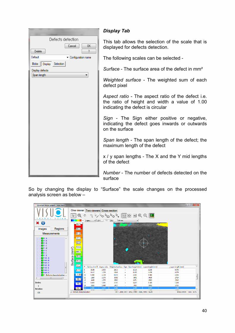
Display Tab This tab allows the selection of the scale that is displayed for defects detection. The following scales can be selected - Surface - The surface area of the defect in mm² Weighted surface - The weighted sum of each defect pixel Aspect ratio - The aspect ratio of the defect i.e. the ratio of height and width a value of 1.00 indicating the defect is circular Sign - The Sign either positive or negative, indicating the defect goes inwards or outwards on the surface Span length - The span length of the defect; the maximum length of the defect x / y span lengths - The X and the Y mid lengths of the defect Number - The number of defects detected on the surface

So by changing the display to “Surface” the scale changes on the processed analysis screen as below –

41

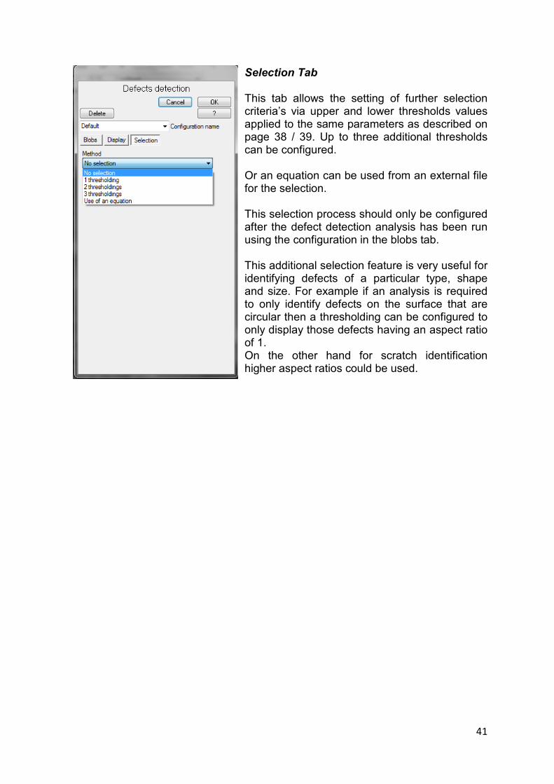
Selection Tab This tab allows the setting of further selection criteria’s via upper and lower thresholds values applied to the same parameters as described on page 38 / 39. Up to three additional thresholds can be configured. Or an equation can be used from an external file for the selection. This selection process should only be configured after the defect detection analysis has been run using the configuration in the blobs tab. This additional selection feature is very useful for identifying defects of a particular type, shape and size. For example if an analysis is required to only identify defects on the surface that are circular then a thresholding can be configured to only display those defects having an aspect ratio of 1. On the other hand for scratch identification higher aspect ratios could be used.