Universit´ e de Li` ege Facult´ e des Sciences Appliqu´ ees On the Verification of Programs on Relaxed Memory Models Th` ese pr´ esent´ ee par Alexander Linden en vue de l’obtention du grade de Docteur en Sciences, orientation Informatique Ann´ ee acad´ emique 2013-2014

Welcome message from author
This document is posted to help you gain knowledge. Please leave a comment to let me know what you think about it! Share it to your friends and learn new things together.
Transcript
Universite de Liege
Faculte des Sciences Appliquees
On the Verification of Programs on
Relaxed Memory Models
These presentee par
Alexander Linden
en vue de l’obtention du grade de
Docteur en Sciences,
orientation Informatique
Annee academique 2013-2014

Abstract
Classical model-checking tools verify concurrent programs under the tra-
ditional Sequential Consistency (SC) memory model, in which all accesses
to the shared memory are immediately visible globally, and where model-
checking consists in verifying a given property when exploring the state
space of a program. However, modern multi-core processor architectures
implement relaxed memory models, such as Total Store Order (TSO), Par-
tial Store Order (PSO), or an extension with locks such as x86-TSO, which
allow stores to be delayed in various ways and thus introduce many more
possible executions, and hence errors, than those present in SC. Of course,
one can force a program executed in the context of a relaxed memory system
to behave exactly as in SC by adding synchronization operations after every
memory access. But this totally defeats the performance advantage that is
precisely the motivation for implementing relaxed memory models instead
of SC. Thus, when moving a program to an architecture implementing a re-
laxed memory model (which includes most current multi-core processors),
it is essential to have tools to help the programmer check if correctness
(e.g. a safety property) is preserved and, if not, to minimally introduce the
necessary synchronization operations.
The proposed verification approach uses an operational store-buffer-based
semantics of the chosen relaxed memory models and proceeds by using finite
automata for symbolically representing the possible contents of the buffers.
Store, load, commit and other synchronization operations then correspond
to operations on these finite automata.
The advantage of this approach is that it operates on (potentially infinite)
sets of buffer contents, rather than on individual buffer configurations, and
that it is compatible with partial-order reduction techniques. This provides
a way to tame the explosion of the number of possible buffer configurations,
while preserving the full generality of the analysis. It is thus possible to
even check designs that may contain cycles.
This verification approach then serves as a basis to a memory fence inser-
tion algorithm that finds how to preserve the correctness of a program when
it is moved from SC to TSO or PSO. Its starting point is a program that
is correct for the sequential consistency memory model (with respect to a
given safety property), but that might be incorrect under TSO or PSO.
This program is then analyzed for the chosen relaxed memory model and
when errors are found (a violated safety property), memory fences are in-
serted in order to avoid these errors. The approach proceeds iteratively and
heuristically, inserting memory fences until correctness is obtained, which
is guaranteed to happen.

Acknowledgements
First of all, I would like to thank my thesis advisor, Pierre Wolper, for
giving me the opportunity to collaborate with him and for introducing me
to the area of program verification, as well as for giving me the time to
freely chose the subject of my research. Without all the fruitful discussions
and encouragements, the content and the presentation of this thesis would
not have been possible.
Next, I need to thank Bernard Boigelot for many discussions, as well as
for funding many travels to conferences and other scientific events. His
previous work on infinite-state systems also need to be mentioned and was
very helpful in developing the content of this thesis. I need to thank him as
well for reading and commenting several parts of this thesis in very short
delays during the final stage of writing.
Thanks to the members of the jury, Bernard Boigelot, Pascal Gribomont,
Jean-Francois Raskin, Ahmed Bouajjani and Martin Vechev, who have ac-
cepted to read and evaluate this thesis.
Other thanks go to all the people I have met during scientific events hav-
ing given me inspiration, ideas and feedback, especially Ahmed Bouajjani,
Faouzi Atig, Roland Meyer and Vincent Nimal. Different approaches have
been discussed pointing out advantages and drawbacks.
Then, I need to thank my colleagues I have spent plenty of time with during
coffee-breaks and lunch-time. Special thanks goes to Julien Brusten who,
beside having been a colleague, is a good friend and accepted to review parts
of this thesis in very short delay, as well as for introducing me to Sushi.
Last but not least, I need to thank my family and friends for their long-
time support. I’m indepted to Lydia for her love during all the years,
being patient and confident, and the most important, for giving birth to
our children and thus a sense to our life.

Contents
Abstract iii
Acknowledgement v
List of Figures xi
List of Tables xiii
List of Algorithms/Procedures xvi
1 Introduction 1
1.1 Motivation . . . . . . . . . . . . . . . . . . . . . . . . . . . . . . . . . . 1
1.2 Overview of Existing Approaches . . . . . . . . . . . . . . . . . . . . . . 3
1.3 Contributions . . . . . . . . . . . . . . . . . . . . . . . . . . . . . . . . . 5
1.4 Outline . . . . . . . . . . . . . . . . . . . . . . . . . . . . . . . . . . . . 6
2 Intel’s Memory Model in Practice 9
2.1 Intel’s White Paper on Memory Ordering . . . . . . . . . . . . . . . . . 9
2.2 Updated Intel Version . . . . . . . . . . . . . . . . . . . . . . . . . . . . 15
2.3 Observations Made on Multi-Core Processors . . . . . . . . . . . . . . . 15
2.4 Discussion . . . . . . . . . . . . . . . . . . . . . . . . . . . . . . . . . . . 17
3 Memory Models and Concurrent Systems 19
3.1 Sequential Consistency (SC) . . . . . . . . . . . . . . . . . . . . . . . . . 20
3.2 Total Store Order (TSO) . . . . . . . . . . . . . . . . . . . . . . . . . . 25
3.3 Partial Store Order (PSO) . . . . . . . . . . . . . . . . . . . . . . . . . . 33
3.4 Extensions with Locks and Memory Fences . . . . . . . . . . . . . . . . 37
3.4.1 Extended TSO: x86-TSO . . . . . . . . . . . . . . . . . . . . . . 37
vii
CONTENTS
3.4.2 Extended PSO . . . . . . . . . . . . . . . . . . . . . . . . . . . . 40
3.5 Discussion on SC, TSO, PSO, their Extensions and Other Memory Models 43
4 Ingredients to our Approach 47
4.1 Verification of Programs . . . . . . . . . . . . . . . . . . . . . . . . . . . 47
4.2 Partial-Order Reduction . . . . . . . . . . . . . . . . . . . . . . . . . . . 50
4.2.1 Independent Transitions . . . . . . . . . . . . . . . . . . . . . . . 51
4.2.2 Persistent-Sets . . . . . . . . . . . . . . . . . . . . . . . . . . . . 52
4.2.3 Sleep-Sets . . . . . . . . . . . . . . . . . . . . . . . . . . . . . . . 53
4.2.4 On Combining Persistent-Sets and Sleep-Sets . . . . . . . . . . . 55
4.3 Computing Infinite State Spaces . . . . . . . . . . . . . . . . . . . . . . 58
4.4 Buffer Automata . . . . . . . . . . . . . . . . . . . . . . . . . . . . . . . 59
5 Total Store Order 65
5.1 Buffer Operations . . . . . . . . . . . . . . . . . . . . . . . . . . . . . . . 66
5.1.1 Store Operation . . . . . . . . . . . . . . . . . . . . . . . . . . . 66
5.1.2 Load check Operation . . . . . . . . . . . . . . . . . . . . . . . . 67
5.1.3 Load Operation . . . . . . . . . . . . . . . . . . . . . . . . . . . . 70
5.1.4 Commit Operation . . . . . . . . . . . . . . . . . . . . . . . . . . 71
5.1.5 Mfence Operation . . . . . . . . . . . . . . . . . . . . . . . . . . 72
5.1.6 Lock Operation . . . . . . . . . . . . . . . . . . . . . . . . . . . . 73
5.1.7 Unlock Operation . . . . . . . . . . . . . . . . . . . . . . . . . . 74
5.1.8 Local Operation . . . . . . . . . . . . . . . . . . . . . . . . . . . 74
5.1.9 Discussion on Operations . . . . . . . . . . . . . . . . . . . . . . 74
5.2 Cycles . . . . . . . . . . . . . . . . . . . . . . . . . . . . . . . . . . . . . 75
5.2.1 Cycle Acceleration in Theory . . . . . . . . . . . . . . . . . . . . 76
5.2.2 Cycle Acceleration Algorithm . . . . . . . . . . . . . . . . . . . . 83
5.2.3 Termination . . . . . . . . . . . . . . . . . . . . . . . . . . . . . . 94
5.3 Partial-Order Reduction . . . . . . . . . . . . . . . . . . . . . . . . . . . 97
5.3.1 Independence Relation . . . . . . . . . . . . . . . . . . . . . . . . 97
5.3.1.1 Transitions of the Same Process . . . . . . . . . . . . . 98
5.3.1.2 Transitions of Different Processes . . . . . . . . . . . . 100
5.3.2 Persistent-Sets . . . . . . . . . . . . . . . . . . . . . . . . . . . . 105
5.3.3 Sleep-Sets . . . . . . . . . . . . . . . . . . . . . . . . . . . . . . . 109
viii
CONTENTS
5.3.4 Depth-First Search by Combining Partial-Order Reduction and
Cycle Acceleration in TSO . . . . . . . . . . . . . . . . . . . . . 111
5.4 Deadlock Detection . . . . . . . . . . . . . . . . . . . . . . . . . . . . . . 117
5.5 Safety Property Verification . . . . . . . . . . . . . . . . . . . . . . . . . 119
5.6 Moving from SC to TSO . . . . . . . . . . . . . . . . . . . . . . . . . . . 122
5.6.1 Error Correction: Iterative Memory Fence Insertion . . . . . . . 123
6 Partial Store Order 127
6.1 Buffer Operations . . . . . . . . . . . . . . . . . . . . . . . . . . . . . . . 128
6.1.1 Store Operation . . . . . . . . . . . . . . . . . . . . . . . . . . . 128
6.1.2 Load check Operation . . . . . . . . . . . . . . . . . . . . . . . . 129
6.1.3 Load Operation . . . . . . . . . . . . . . . . . . . . . . . . . . . . 131
6.1.4 Commit Operation . . . . . . . . . . . . . . . . . . . . . . . . . . 133
6.1.5 Mfence Operation . . . . . . . . . . . . . . . . . . . . . . . . . . 134
6.1.6 Sfence Operation . . . . . . . . . . . . . . . . . . . . . . . . . . . 134
6.1.7 Lock Operation . . . . . . . . . . . . . . . . . . . . . . . . . . . . 135
6.1.8 Unlock Operation . . . . . . . . . . . . . . . . . . . . . . . . . . 135
6.1.9 Local Operation . . . . . . . . . . . . . . . . . . . . . . . . . . . 136
6.1.10 Discussion on Operations . . . . . . . . . . . . . . . . . . . . . . 136
6.2 Cycles . . . . . . . . . . . . . . . . . . . . . . . . . . . . . . . . . . . . . 136
6.3 Partial-Order Reduction . . . . . . . . . . . . . . . . . . . . . . . . . . . 139
6.3.1 Independence Relation . . . . . . . . . . . . . . . . . . . . . . . . 139
6.3.1.1 Transitions of the Same Process . . . . . . . . . . . . . 139
6.3.1.2 Transitions of Different Processes . . . . . . . . . . . . 140
6.3.2 Persistent-Sets and Sleep-Sets . . . . . . . . . . . . . . . . . . . . 142
6.4 Deadlock Detection and Safety Property Verification . . . . . . . . . . . 143
6.5 Moving from SC to TSO to PSO . . . . . . . . . . . . . . . . . . . . . . 143
6.5.1 Error Correction: Iterative Memory Fence Insertion . . . . . . . 145
7 Remmex : RElaxed Memory Model EXplorer 149
7.1 The Tool: Remmex . . . . . . . . . . . . . . . . . . . . . . . . . . . . . . 149
7.1.1 Input Language . . . . . . . . . . . . . . . . . . . . . . . . . . . . 149
7.1.2 Features . . . . . . . . . . . . . . . . . . . . . . . . . . . . . . . . 152
7.2 Experiments . . . . . . . . . . . . . . . . . . . . . . . . . . . . . . . . . . 154
ix
CONTENTS
8 Conclusions 165
8.1 Summary . . . . . . . . . . . . . . . . . . . . . . . . . . . . . . . . . . . 165
8.2 Related Work . . . . . . . . . . . . . . . . . . . . . . . . . . . . . . . . . 166
8.3 Future Work . . . . . . . . . . . . . . . . . . . . . . . . . . . . . . . . . 170
A Example Programs 171
A.1 Mutual Exclusion Algorithms . . . . . . . . . . . . . . . . . . . . . . . . 171
A.1.1 Dekker . . . . . . . . . . . . . . . . . . . . . . . . . . . . . . . . . 171
A.1.2 Peterson . . . . . . . . . . . . . . . . . . . . . . . . . . . . . . . . 173
A.1.3 Generalized Peterson . . . . . . . . . . . . . . . . . . . . . . . . . 173
A.1.4 Lamport’s Fast Mutex . . . . . . . . . . . . . . . . . . . . . . . . 176
A.1.5 Dijkstra . . . . . . . . . . . . . . . . . . . . . . . . . . . . . . . . 176
A.1.6 Burns . . . . . . . . . . . . . . . . . . . . . . . . . . . . . . . . . 176
A.1.7 Szymanski . . . . . . . . . . . . . . . . . . . . . . . . . . . . . . . 176
A.1.8 Lamport’s Bakery . . . . . . . . . . . . . . . . . . . . . . . . . . 177
A.2 TSO/PSO-Safe Programs . . . . . . . . . . . . . . . . . . . . . . . . . . 177
A.2.1 Alternating Bit Protocol . . . . . . . . . . . . . . . . . . . . . . . 177
A.2.2 CLH Queue Lock . . . . . . . . . . . . . . . . . . . . . . . . . . . 178
A.2.3 Increasing Sequence . . . . . . . . . . . . . . . . . . . . . . . . . 178
A.3 Different Types of Cycles . . . . . . . . . . . . . . . . . . . . . . . . . . 178
A.3.1 Mixable Cycles . . . . . . . . . . . . . . . . . . . . . . . . . . . . 178
A.3.2 Mixable Cycles 2 . . . . . . . . . . . . . . . . . . . . . . . . . . . 179
A.3.3 Cycle Unlocking Example . . . . . . . . . . . . . . . . . . . . . . 179
A.4 Program with Deadlock under TSO/PSO . . . . . . . . . . . . . . . . . 179
A.5 TSO-Safe Program Not being PSO-Safe . . . . . . . . . . . . . . . . . . 180
Bibliography 193
x
List of Figures
3.1 Operational definition of SC. . . . . . . . . . . . . . . . . . . . . . . . . 22
3.2 Operational definition of TSO. . . . . . . . . . . . . . . . . . . . . . . . 26
3.3 Operational definition of PSO. . . . . . . . . . . . . . . . . . . . . . . . 34
3.4 Operational definition of x86-TSO. . . . . . . . . . . . . . . . . . . . . . 38
3.5 Inclusion relation between SC, TSO and PSO in terms of allowed exe-
cutions. . . . . . . . . . . . . . . . . . . . . . . . . . . . . . . . . . . . . 44
4.1 Control graph of two processes of a program. . . . . . . . . . . . . . . . 56
4.2 Full state space of the program. . . . . . . . . . . . . . . . . . . . . . . . 56
4.3 State space of the program reduced by persistent-sets. . . . . . . . . . . 57
4.4 State space of the program reduced by sleep-sets. . . . . . . . . . . . . . 57
4.5 State space of the program reduced by persistent-sets and sleep-sets. . . 58
4.6 Example program showing basic cycle. . . . . . . . . . . . . . . . . . . . 61
4.7 Buffer automaton representing a set of unbounded buffer contents. . . . 62
5.1 Illustration of the TSO store operation. . . . . . . . . . . . . . . . . . . 67
5.2 Illustration of the TSO load check operation. . . . . . . . . . . . . . . . 69
5.3 Illustration of the TSO commit operation. . . . . . . . . . . . . . . . . . 72
5.4 Illustration of the TSO mfence operation. . . . . . . . . . . . . . . . . . 73
5.5 Buffer automaton of process p in state s of Algorithm 6. . . . . . . . . . 83
5.6 Buffer automata corresponding to the mixable sequences of Algorithm 6. 83
5.7 Buffer automaton after acceleration of the mixable sequences. . . . . . . 84
5.8 Partial state space of the program given in Algorithm 6. . . . . . . . . . 94
5.9 Buffer automaton accepting those words of the language in Equation 5.2. 100
5.10 Control graphs of two processes p0 and p1. . . . . . . . . . . . . . . . . . 114
xi
LIST OF FIGURES
5.11 Partial state space of the program in Fig. 5.10. . . . . . . . . . . . . . . 114
6.1 A program with writes to different variables in a cycle . . . . . . . . . . 137
A.1 Control graphs of the first process in Dekker’s algorithm for mutual
exclusion. . . . . . . . . . . . . . . . . . . . . . . . . . . . . . . . . . . . 173
A.2 Control graph of the second process in Dekker’s algorithm for mutual
exclusion . . . . . . . . . . . . . . . . . . . . . . . . . . . . . . . . . . . 174
xii
List of Tables
2.1 Loads are not reordered with other loads and stores are not reordered
with other stores. . . . . . . . . . . . . . . . . . . . . . . . . . . . . . . . 11
2.2 Stores are not reordered with older loads. . . . . . . . . . . . . . . . . . 11
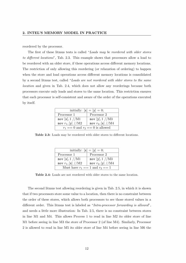
2.3 Loads may be reordered with older stores to different locations. . . . . . 12
2.4 Loads are not reordered with older stores to the same location. . . . . . 12
2.5 Intra-processor forwarding is allowed. . . . . . . . . . . . . . . . . . . . . 13
2.6 Stores are transitively visible. . . . . . . . . . . . . . . . . . . . . . . . . 13
2.7 Total order on stores to the same location. . . . . . . . . . . . . . . . . . 13
2.8 Independent Read Independent Write. . . . . . . . . . . . . . . . . . . . 14
3.1 Intra-processor forwarding is allowed from [37]. . . . . . . . . . . . . . . 29
3.2 Possible operation sequence and memory order for Tab. 3.1. . . . . . . . 30
3.3 Operational execution of example in Tab. 3.1. . . . . . . . . . . . . . . . 33
3.4 Example program with possible store-store relaxation. . . . . . . . . . . 36
3.5 Possible operation sequence and memory order for Tab. 3.4. . . . . . . . 37
5.1 Description of the partially explored state space of Fig. 5.8. . . . . . . . 93
5.2 Description of the partially explored state space of Fig. 5.11 . . . . . . . 113
7.1 BNF of our input language based on Promela. . . . . . . . . . . . . . . . 151
7.2 Experimental results for mutual exclusion algorithms computing the
whole state space under TSO. . . . . . . . . . . . . . . . . . . . . . . . . 156
7.3 Experimental results for mutual exclusion algorithms under TSO when
errors are iteratively corrected. . . . . . . . . . . . . . . . . . . . . . . . 157
xiii
LIST OF TABLES
7.4 Experimental results for mutual exclusion algorithms under TSO when
errors are iteratively corrected and where the fence set is ensured to be
maximal permissive. . . . . . . . . . . . . . . . . . . . . . . . . . . . . . 157
7.5 Experimental results for mutual exclusion algorithms computing the
whole state space under SC with SPIN. . . . . . . . . . . . . . . . . . . 158
7.6 Experimental results for several TSO-safe programs computing the whole
state space under TSO. . . . . . . . . . . . . . . . . . . . . . . . . . . . 158
7.7 Experimental results for several TSO-safe programs computing the whole
state space under SC using SPIN. . . . . . . . . . . . . . . . . . . . . . . 159
7.8 Experimental results for some programs under TSO with different cycle
types. . . . . . . . . . . . . . . . . . . . . . . . . . . . . . . . . . . . . . 159
7.9 Experimental results for a program having a deadlock under TSO but
not under SC. . . . . . . . . . . . . . . . . . . . . . . . . . . . . . . . . . 160
7.10 Experimental results for mutual exclusion algorithms computing the
whole state space under PSO. . . . . . . . . . . . . . . . . . . . . . . . . 160
7.11 Experimental results for mutual exclusion algorithms under PSO when
errors are iteratively corrected. . . . . . . . . . . . . . . . . . . . . . . . 161
7.12 Experimental results for mutual exclusion algorithms under PSO when
errors are iteratively corrected where the fence sets are ensured to be
maximal permissive. . . . . . . . . . . . . . . . . . . . . . . . . . . . . . 162
7.13 Experimental results for several PSO-safe programs computing the whole
state space under PSO. . . . . . . . . . . . . . . . . . . . . . . . . . . . 162
7.14 Experimental results for some programs under PSO with different cycle
types. . . . . . . . . . . . . . . . . . . . . . . . . . . . . . . . . . . . . . 162
7.15 Experimental results for a program having a deadlock under PSO but
not under SC. . . . . . . . . . . . . . . . . . . . . . . . . . . . . . . . . . 163
xiv
List of algorithms/procedures
1 Peterson’s algorithm for mutual exclusion . . . . . . . . . . . . . . . . . 16
2 Illustration of the two ways of modeling a wait operation. . . . . . . . . 24
3 Initialization and first call of depth-first search. . . . . . . . . . . . . . . 49
4 DFS(): Basic depth-first search procedure. . . . . . . . . . . . . . . . . . 50
5 DFS POR(): Depth-first search procedure using partial-order reduction. 55
6 Example program with three mixable sequences to accelerate. . . . . . . 82
7 Outline of cycle detection and introduction algorithm. . . . . . . . . . . 85
8 Cycle detection procedure (step 2 and 3 of Algorithm 7). . . . . . . . . . 88
9 Detection of mixable sequences detected in a row (used in steps 3 and 4
of Algorithm 7). . . . . . . . . . . . . . . . . . . . . . . . . . . . . . . . 89
10 Program not possible to accelerate by our technique. . . . . . . . . . . . 96
11 Program unlocking a cycle in Algorithm 10. . . . . . . . . . . . . . . . . 96
12 Persistent-set computation in a state s. . . . . . . . . . . . . . . . . . . 107
13 Sleep-set updating with symbolic states. . . . . . . . . . . . . . . . . . . 110
14 DFS POR ACC() - Depth-first search procedure using partial-order re-
duction and cycle acceleration. . . . . . . . . . . . . . . . . . . . . . . . 117
15 Outline of the iterative mfence insertion algorithm. . . . . . . . . . . . . 124
16 Iterative mfence insertion algorithm. . . . . . . . . . . . . . . . . . . . . 124
17 DFS POR ACC MFENCE INSERTION() - Depth-first search procedure
using partial-order reduction and cycle acceleration with error detection
and correction. . . . . . . . . . . . . . . . . . . . . . . . . . . . . . . . . 125
18 Outline of iterative mfence/sfence insertion algorithm. . . . . . . . . . . 145
19 Peterson’s algorithm for mutual exclusion: input file. . . . . . . . . . . . 152
20 Dekker’s algorithm for mutual exclusion. . . . . . . . . . . . . . . . . . . 172
21 Peterson’s algorithm for mutual exclusion. . . . . . . . . . . . . . . . . . 174
xv
LIST OF ALGORITHMS/PROCEDURES
22 Generalized Peterson’s algorithm for mutual exclusion with three processes.175
23 Lamport’s Fast Mutex instantiated for two processes. . . . . . . . . . . . 181
24 Dijkstra’s algorithm for mutual exclusion instantiated for two processes. 182
25 Burns algorithm for mutual exclusion instantiated for two processes. . . 183
26 Szymanski’s algorithm for mutual exclusion instantiated for two processes.184
27 Lamport’s Bakery for mutual exclusion instantiated for two processes. . 185
28 Lamport’s Bakery for mutual exclusion instantiated for three processes. 186
29 Alternating bit protocol simulated by shared variables instead of message
channels. . . . . . . . . . . . . . . . . . . . . . . . . . . . . . . . . . . . 187
30 CLH queue lock mutual exclusion algorithm. . . . . . . . . . . . . . . . 188
31 Increasing sequence. . . . . . . . . . . . . . . . . . . . . . . . . . . . . . 189
32 Program with two mixable cycles. . . . . . . . . . . . . . . . . . . . . . . 189
33 Program with three cycles among which two are mixable. . . . . . . . . 190
34 Cycle unlocking example. . . . . . . . . . . . . . . . . . . . . . . . . . . 190
35 Program with a deadlock under TSO/PSO, but not under SC. . . . . . 191
36 Program with a deadlock under PSO, but not under SC/TSO. . . . . . 192
xvi
Chapter 1
Introduction
1.1 Motivation
According to Moore’s Law the number of transistors on integrated circuits doubles
every two years, and as the speed of those transistors also increases, the computation
power of processors doubles every 18 month. This has led to such large capacities
for chips that placing several processors onto a single chip which share some common
circuits, called a multi-core processor, is now routine. But to unleash the full power
of a such a processor, programmers need to write concurrent programs in which tasks
are divided into several threads, with different threads (or processes) being executed
on different processor cores. Communication between the different threads is usually
done through shared memory, and this is where difficulties start.
Indeed, the shared memory units of multi-core processors behave in specific ways
defined in what is called the Memory Model. Different processor families have different
memory models, each one leading to different behaviors. The classical memory model,
known as Sequential Consistency (SC) [43], is also the strongest: all memory accesses
become visible to all cores directly after being executed. In weaker memory models,
known as relaxed memory models, memory accesses can be delayed in different ways,
for example by allowing stores to be buffered in a store buffer of the core, and thus to
be delayed, and appear to be executed after subsequent loads. Memory accesses can
thus be reordered, where the allowed reorderings are defined by the memory model.
Verifying programs, for example using the model-checker SPIN [34], under the clas-
sical memory model is already not an easy task, but verifying them under relaxed mem-
1
1. INTRODUCTION
ory models is even more difficult. A model-checker like SPIN verifies that a property
is satisfied by a program by exploring its whole state space, while checking if the prop-
erty is satisfied or not. When considering the classical sequential consistency memory
model, the state space of a concurrent program is obtained by computing all possible
interleavings of the instructions of the different processes. This already often leads to
a very large, frequently impossible to compute, state space, a phenomenon known as
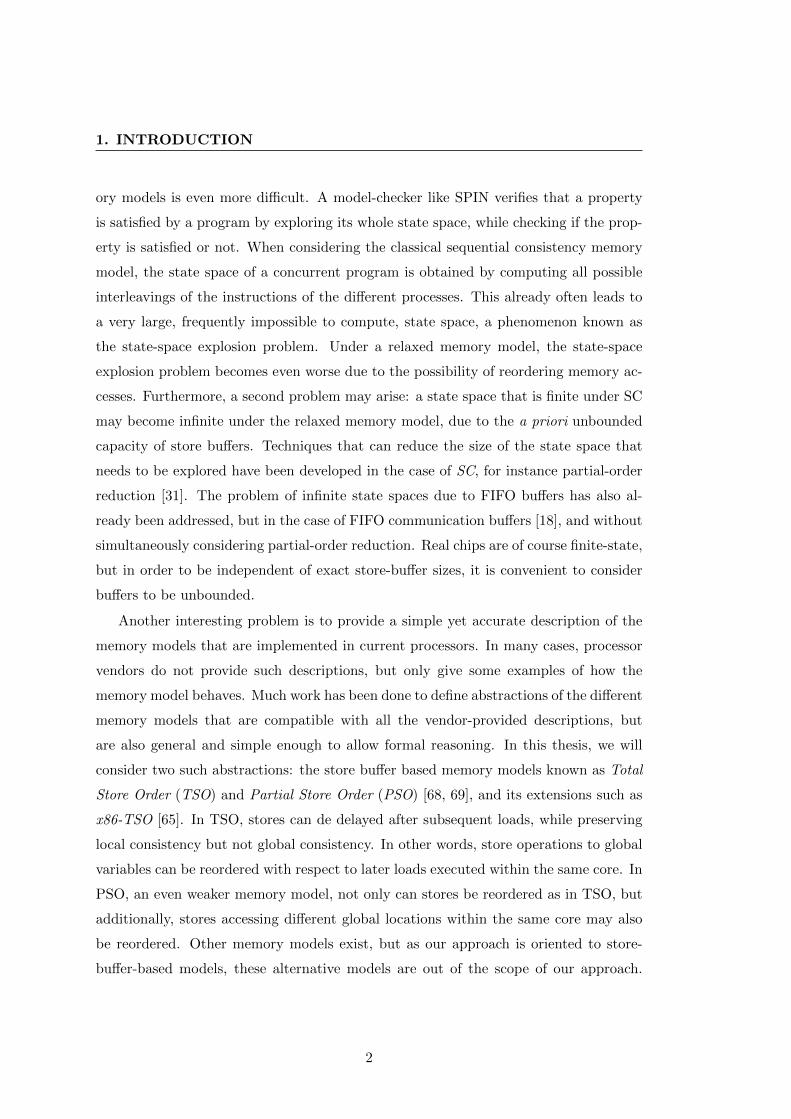
the state-space explosion problem. Under a relaxed memory model, the state-space
explosion problem becomes even worse due to the possibility of reordering memory ac-
cesses. Furthermore, a second problem may arise: a state space that is finite under SC
may become infinite under the relaxed memory model, due to the a priori unbounded
capacity of store buffers. Techniques that can reduce the size of the state space that
needs to be explored have been developed in the case of SC, for instance partial-order
reduction [31]. The problem of infinite state spaces due to FIFO buffers has also al-
ready been addressed, but in the case of FIFO communication buffers [18], and without
simultaneously considering partial-order reduction. Real chips are of course finite-state,
but in order to be independent of exact store-buffer sizes, it is convenient to consider
buffers to be unbounded.
Another interesting problem is to provide a simple yet accurate description of the
memory models that are implemented in current processors. In many cases, processor
vendors do not provide such descriptions, but only give some examples of how the
memory model behaves. Much work has been done to define abstractions of the different
memory models that are compatible with all the vendor-provided descriptions, but
are also general and simple enough to allow formal reasoning. In this thesis, we will
consider two such abstractions: the store buffer based memory models known as Total
Store Order (TSO) and Partial Store Order (PSO) [68, 69], and its extensions such as
x86-TSO [65]. In TSO, stores can de delayed after subsequent loads, while preserving
local consistency but not global consistency. In other words, store operations to global
variables can be reordered with respect to later loads executed within the same core. In
PSO, an even weaker memory model, not only can stores be reordered as in TSO, but
additionally, stores accessing different global locations within the same core may also
be reordered. Other memory models exist, but as our approach is oriented to store-
buffer-based models, these alternative models are out of the scope of our approach.
2
1.2 Overview of Existing Approaches
However, knowing that Intel’s multi-core processors are correctly modeled by the x86-
TSO memory model [65], our approach covers an important part of the processors
that are currently used. Other memory models are RMO (relaxed memory order) [69],
PowerPC [55] and many more [54].
Finally, when programmers design a program satisfying a given property, they
mostly think in terms of SC instead of a relaxed memory model. When such a program
is then executed on a real computer (a modern multi-core processor), one needs to
check if the program still satisfies the property on that processor, and if not, to provide
a way to modify the program for the property to be preserved when the program is
moved onto that processor. This is done by forcing synchronization at given points,
using instructions known as fences. Several approaches that lead to that goal, manual
or automatic, more or less complex, optimal or not, have been proposed. We review
them in the next section.
1.2 Overview of Existing Approaches
For the store-buffer-based memory models TSO and PSO, a natural choice is to include
the store buffers explicitly into the description of the system. Many approaches have
adopted this strategy. In [41], an over-abstraction technique for potentially infinite
store buffers is proposed and is combined with the fence insertion algorithm described as
“maximal permissive” that was presented in [40]. The abstraction works by representing
the buffers as a combination of a finite FIFO buffer that keeps the order of the stores,
and of an unordered set of stores that is used when the FIFO buffer is full. The fence
inference technique works by propagating through the state space constraints that
represent relaxations that can be removed if necessary by inserting fences. Once an
undesirable state has been reached, one can use the associated constraints in order to
determine how to make that state unreachable for all incoming paths. However, even if
the state space that is computed is finite in theory, the number of states grows very fast,
even for very simple programs, which was even confirmed by the same authors in [48]
where an adapted approach of [41] is presented. Another approach consists in applying
some under-approximation in order to keep the store buffers finite. In [13], such an
under-approximation is applied when either bounding the number of context-switches
of the different processes or bounding the time a given store operation can be buffered
3
1. INTRODUCTION
in the store buffers. Other work on verification under relaxed memory models includes
[24], which proceeds by detecting behaviors that are not allowed by SC but might occur
under TSO (or PSO). This is done by only exploring SC interleavings of the program,
and by using explicit store buffers. Yet a different approach can be found in [39], which
proposes an approach based on SPIN that uses a Promela (the modeling language
of SPIN) model with (bounded) explicit queues and an explicit representation of the
memory-access-dependencies that are implied by the relaxed model RMO. One of the
earliest pieces of work on the subject is the one presented in [61], where the problem was
clearly defined and where it was shown that behaviors possible under TSO but not SC
can be detected by an explicit state model checker. Another piece of early work is [64],
where a model-checking algorithm aimed at verifying whether sequential consistency
is preserved while moving to a weak memory system is proposed. It is applicable to
programs using a finite number of processors and memory locations, but manipulating
an arbitrary number of data values.
The more theoretical work presented in [11] uses results about systems with lossy
channel systems, by simulating TSO/PSO system by lossy channel systems and vice-
versa, in order to prove decidability of reachability under TSO (or PSO) with respect to
unbounded store buffers, but undecidability of repeated reachability. In later work [12]
of the same authors, an even finer characterization of the border between decidability
and undecidability of various problems with respect to different relaxations is presented.
The work in [1] and [2] exploits the fact that TSO can be simulated by lossy channel
systems. The advantage is that, in this setting, state reachability is decidable by a
procedure that can be implemented quite efficiently. This approach, combined with a
fence insertion algorithm that computes all maximal permissive fence sets, by optionally
restricting the places in the program where fence insertion is allowed, makes it very
efficient in the case of TSO. It is worth mentioning that their technique for computing
the minimal fence sets is compatible with our approach in the case of TSO, as we will
describe later in this thesis.
Other approaches to verification, with respect to relaxed memory models, adopt the
axiomatic definition of these models and exploit SAT-based bounded model checking
[22, 23]. In bounded model checking, the state spaces to handle are finite-state, hence
only bounded store-buffers are considered.
4
1.3 Contributions
The last type of approach proceeds by only exploring SC-executions while looking
for the possibility of breaking out of the SC-execution. This is known as the problem
of deciding whether a program is robust against a given memory model. All those
contributions are based on the definitions given in [66], where a happens-before relation
between operations is used to prove either robustness, if the happens-before relation
is non-cyclic, or non-robustness, if the happens-before relation is cyclic. Contributions
following this approach are [23], [8, 9, 10] and [20, 21]. Also, in this line of work,
breaking the cycles in the happens-before relation can be enforced by placing fences
into the program, hence making the program robust. The advantage of that type of
approach is that it scales better than approaches exploring the state space using store
buffers. The drawback is that the sets of fences are potentially bigger than needed
with respect to preserving a given property, since all executions deviating from SC are
disabled, not just those leading to a state violating the required property.
1.3 Contributions
The main contribution of this thesis is to provide an alternative way to verify pro-
grams with respect to safety properties under the TSO and PSO memory models.
We will mainly consider programs that are finite-state under SC, and which can turn
into infinite-state programs when considering TSO or PSO as the underlying memory
system.
The verification of those programs is basically performed with a classical depth-
first search state-space exploration, enriched by several techniques, namely symbolic
representation of the store buffers, cycle acceleration by cycle detection and cycle in-
troduction into the symbolic store buffers, as well as partial-order reductions to limit
the size of the state space.
The symbolic representation of the store buffers, a data structure called buffer
automata, are finite-state automata, where the alphabet will be composed of the store
operations executed by the program. By using these buffer automata, we will be able
to represent sets of unbounded buffer contents using a finite structure. The program
operations involving the shared memory are mapped onto operations handling the buffer
automata. Additionally, to unleash the power of the buffer automata, we will present a
technique that can detect a specific type of cycles, those than most commonly lead to
5
1. INTRODUCTION
an infinite state space under the relaxed memory model. Once such a cycle is detected,
the buffer automata will be modified in such a way that it represents all buffer contents
that are possible after the repeated execution of the cycle. Thus, we can get a finite
structure symbolically representing an infinite set of buffer contents. This makes it
possible to represent an infinite number of global states within a single symbolic state.
These concepts have been introduced in [45] for TSO, and were extended to PSO in [47].
Last but not least, in order to be able to correct a program, when a safety property
is violated as the program is moved from SC to TSO/PSO, we will also present an
iterative algorithm that inserts fences into the program until the safety property holds
again, which is guaranteed to happen. This technique has been introduced in [46] when
considering TSO, and has been extended to PSO in [47].
1.4 Outline
Chapter 2 briefly introduces how Intel’s x86 memory models is defined, showcasing the
difficulty of correctly understanding those models.
In Chapter 3, we will give all needed definitions about the memory models that
are considered within this thesis, and formalize the behavior of concurrent systems
operating on those memory models.
In Chapter 4, a series of known techniques that will be used in our approach are pre-
sented. First, a short introduction to the verification of programs is provided. Then,
partial-order reduction techniques are presented; these allow the state space to be
reduced by exploiting the independence between instructions, while preserving all im-
portant behaviors with respect to a given property. Last but not least, the symbolic
data structure allowing us to represent sets of unbounded buffer contents in a finite
way is introduced.
Chapter 5 describes the central results of this document for the TSO memory model.
First, all memory operations are extended from FIFO store buffers to buffer automata.
Next comes the presentation of the cycle acceleration technique which allows the finite
exploration of a system which has become infinite-state due to the introduction of store
buffers. Following this, it is shown that partial-order reduction techniques can safely
be used when combined with our cycle acceleration technique. Finally, our technique
6
1.4 Outline
for modifying programs that are correct with respect to safety properties under SC but
incorrect when moved onto a TSO system is presented.
Chapter 6 extends all techniques provided in Chapter 5 to the PSO memory model,
which turned out to be quite easy.
In Chapter 7, we present the prototype tool implementing the techniques devel-
oped within this document and describe its input-language, as well as all available
options. Thereafter, the experimental results obtained using our tool are presented.
A comparison with results obtained by using the model checker SPIN when SC is the
memory model is given, providing interesting results. It turns out that the use of store-
buffers introduces a lot of independence between the transitions of the system which is
exploited by the partial-order reduction we use.
Finally, Chapter 8 concludes this thesis and Appendix A provides all programs used
for the experimental results.
7

Chapter 2
Intel’s Memory Model in Practice
This chapter introduces how memory models are defined in practice by processor ven-
dors, illustrated by Intel’s definition of the x86 memory model. This definition is not
a formal one, it only gives the intuition about what can happen or not, illustrated by
some short examples. Unsurprisingly, this informal style leads to ambiguous situations
in which the programmer does not know how the multi-core processor will behave, or
more precisely, how the multi-core processor could behave. This shows the importance
of providing good definitions of memory models in order to allow programmers to un-
leash the full power of modern processors without unnecessarily restricting them by
compensating lack of information with the insertion of needless and expensive synchro-
nization operations.
Several formal definitions of memory models have been proposed, and processor
vendors have improved their definitions, though still without being formal. In this
chapter, we will give a first introduction to the topic, introducing basic ideas about
the meaning of memory models, as well as discussing observability of the properties of
memory models, and the problems arising from their imprecise definition.
Our focus is on Intel processors, but a similar analysis can be done for AMD pro-
cessors and other manufacturer’s.
2.1 Intel’s White Paper on Memory Ordering
The Intel® 64 Architecture Memory Ordering White Paper, [37], introduced an early
definition of the memory model implemented on x86 multi-core processors. This defini-
9
2. INTEL’S MEMORY MODEL IN PRACTICE
tion was based on eight principles supported by ten examples (litmus tests) of parallel
processor instruction sequences and associated allowed or forbidden behaviors. How-
ever, those principles combined with the examples let some room for interpretation on
how the processor can behave, and the authors of [60, 65] pointed out the weaknesses
of these definition.
Before following their argumentation, we need to introduce the eight principles Intel
gave in that White Paper:
1. Loads are not reordered with other loads.
2. Stores are not reordered with other stores.
3. Stores are not reordered with older loads.1
4. Loads may be reordered with older stores to different locations but not with older
stores to the same location.
5. In a multiprocessor system, memory ordering obeys causality (memory ordering
respects transitive visibility).
6. In a multiprocessor system, stores to the same location have a global order.
7. In a multiprocessor system, locked instructions have a total order.
8. Loads and stores are not reordered with locked instructions.
The litmus tests use Intel 64 assembly language syntax. The mov instruction serves
as an example of a memory-access instruction, and other memory-access instructions
also obey those principles. Local processor registers have names starting with r, such as
r1 or r2. Shared variables are denoted by x, y or z. Stores are written as “mov [x], val”,
writing val into memory location x. Loads are written as “mov r, [x]”, loading the value
of x into local register r. Lines can be identified by some reference code, often after
the comment marks (//). Each litmus test starts with the list of used shared variables
together with their initial values. Then, a description of the instructions to be executed
by each processor is provided. In a final line, behaviors (or more precisely local register
values) are defined to be allowed or forbidden after executing all instructions of all
processors.
1An operation op1 is older than operation op2 if op1 appears before op2 in the executed program.
10
2.1 Intel’s White Paper on Memory Ordering
We will omit examples considering locked instructions, as both the last two rules
clearly say that there is a total order over all locked instructions and that no load or
store can be reordered with any locked instruction, implying directly that there is no
possible reordering involving a locked instruction, and thus no unexpected behavior
allowed. Three of the examples contain locked instructions, which leaves us seven of
those examples to describe. For each of the examples, we give it the name that was
attributed by Intel.
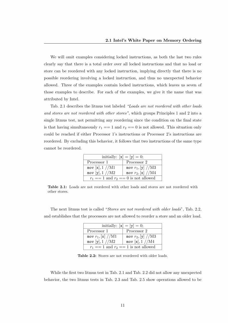
Tab. 2.1 describes the litmus test labeled “Loads are not reordered with other loads
and stores are not reordered with other stores”, which groups Principles 1 and 2 into a
single litmus test, not permitting any reordering since the condition on the final state
is that having simultaneously r1 == 1 and r2 == 0 is not allowed. This situation only
could be reached if either Processor 1’s instructions or Processor 2’s instructions are
reordered. By excluding this behavior, it follows that two instructions of the same type
cannot be reordered.
initially: [x] = [y] = 0;
Processor 1 Processor 2
mov [x], 1 //M1 mov r1, [y] //M3mov [y], 1 //M2 mov r2, [x] //M4
r1 == 1 and r2 == 0 is not allowed
Table 2.1: Loads are not reordered with other loads and stores are not reordered withother stores.
The next litmus test is called “Stores are not reordered with older loads”, Tab. 2.2,
and establishes that the processors are not allowed to reorder a store and an older load.
initially: [x] = [y] = 0;
Processor 1 Processor 2
mov r1, [x] //M1 mov r2, [y] //M3mov [y], 1 //M2 mov [x], 1 //M4
r1 == 1 and r2 == 1 is not allowed
Table 2.2: Stores are not reordered with older loads.
While the first two litmus test in Tab. 2.1 and Tab. 2.2 did not allow any unexpected
behavior, the two litmus tests in Tab. 2.3 and Tab. 2.5 show operations allowed to be
11
2. INTEL’S MEMORY MODEL IN PRACTICE
reordered by the processor.
The first of these litmus tests is called “Loads may be reordered with older stores
to different locations”, Tab. 2.3. This example shows that processors allow a load to
be reordered with an older store, if these operations access different memory locations.
The restriction of only allowing this reordering (or relaxation of ordering) to happen
when the store and load operations access different memory locations is consolidated
by a second litmus test, called “Loads are not reordered with older stores to the same
location and given in Tab. 2.4, which does not allow any reorderings because both
processors execute only loads and stores to the same location. This restriction ensures
that each processor is self-consistent and aware of the order of the operations executed
by itself.
initially: [x] = [y] = 0;
Processor 1 Processor 2
mov [x], 1 //M1 mov [y], 1 //M3mov r1, [y] //M2 mov r2, [x] //M4
r1 == 0 and r2 == 0 is allowed
Table 2.3: Loads may be reordered with older stores to different locations.
initially: [x] = [y] = 0;
Processor 1 Processor 2
mov [x], 1 //M1 mov [y], 1 //M3mov r1, [x] //M2 mov r2, [y] //M4
Must have r1 == 1 and r2 == 1
Table 2.4: Loads are not reordered with older stores to the same location.
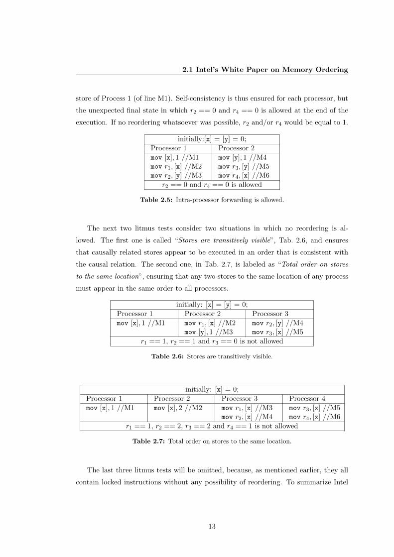
The second litmus test allowing reordering is given in Tab. 2.5, in which it is shown
that if two processors store some value to a location, then there is no constraint between
the order of these stores, which allows both processors to see those stored values in a
different order. This litmus test is labeled as “Intra-processor forwarding is allowed”,
and needs a little more illustration: In Tab. 2.5, there is no constraint between stores
in line M1 and M4. This allows Process 1 to read in line M2 its older store of line
M1 before seeing in line M3 the store of Processor 2 (of line M4). Similarly, Processor
2 is allowed to read in line M5 its older store of line M4 before seeing in line M6 the
12
2.1 Intel’s White Paper on Memory Ordering
store of Process 1 (of line M1). Self-consistency is thus ensured for each processor, but
the unexpected final state in which r2 == 0 and r4 == 0 is allowed at the end of the
execution. If no reordering whatsoever was possible, r2 and/or r4 would be equal to 1.
initially:[x] = [y] = 0;
Processor 1 Processor 2
mov [x], 1 //M1 mov [y], 1 //M4mov r1, [x] //M2 mov r3, [y] //M5mov r2, [y] //M3 mov r4, [x] //M6
r2 == 0 and r4 == 0 is allowed
Table 2.5: Intra-processor forwarding is allowed.
The next two litmus tests consider two situations in which no reordering is al-
lowed. The first one is called “Stores are transitively visible”, Tab. 2.6, and ensures
that causally related stores appear to be executed in an order that is consistent with
the causal relation. The second one, in Tab. 2.7, is labeled as “Total order on stores
to the same location”, ensuring that any two stores to the same location of any process
must appear in the same order to all processors.
initially: [x] = [y] = 0;
Processor 1 Processor 2 Processor 3
mov [x], 1 //M1 mov r1, [x] //M2 mov r2, [y] //M4mov [y], 1 //M3 mov r3, [x] //M5
r1 == 1, r2 == 1 and r3 == 0 is not allowed
Table 2.6: Stores are transitively visible.
initially: [x] = 0;
Processor 1 Processor 2 Processor 3 Processor 4
mov [x], 1 //M1 mov [x], 2 //M2 mov r1, [x] //M3 mov r3, [x] //M5mov r2, [x] //M4 mov r4, [x] //M6
r1 == 1, r2 == 2, r3 == 2 and r4 == 1 is not allowed
Table 2.7: Total order on stores to the same location.
The last three litmus tests will be omitted, because, as mentioned earlier, they all
contain locked instructions without any possibility of reordering. To summarize Intel
13
2. INTEL’S MEMORY MODEL IN PRACTICE
defined the memory model of its processors by giving a list of principles that must
be respected, supported by some example executions illustrating what those principles
might allow and what they might not. However, these litmus tests are not exhaustive,
and the principles leave some space for speculation about what is allowed and what is
not. This was illustrated in [60, 65]. However, even in [37], a hint on how the memory
model could be modeled is given in the section describing “Intra-processor forwarding
is allowed”, where the following is stated:
In practice, the reordering in Table 2.4 1 can arise as a result of store-bufferforwarding. While a store is temporarily held in a processor’s store buffer,it can satisfy the processor’s own loads but is not visible to (and cannotsatisfy) loads on other processors.
Intel® 64 Architecture Memory Ordering White Paper, [37].
This clearly gives an indication that the memory model behaves as an abstract
machine in which each processor might buffer the stores it executes in a store buffer
associated to that processor. All litmus tests can be validated by such an abstract
machine, in particular those in Tab. 2.3 and 2.5, as was also established in [60, 65].
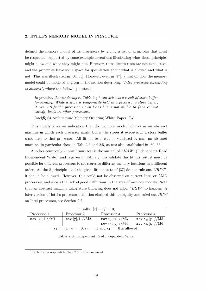
Another commonly known litmus test is the one called “IRIW” (Independent Read
Independent Write), and is given in Tab. 2.8. To validate this litmus test, it must be
possible for different processors to see stores to different memory locations in a different
order. As the 8 principles and the given litmus tests of [37] do not rule out “IRIW”,
it should be allowed. However, this could not be observed on current Intel or AMD
processors, and shows the lack of good definitions in the area of memory models. Note
that an abstract machine using store buffering does not allow “IRIW” to happen. A
later version of Intel’s processor definition clarified this ambiguity and ruled out IRIW
on Intel processors, see Section 2.2.
initially: [x] = [y] = 0;
Processor 1 Processor 2 Processor 3 Processor 4
mov [x], 1 //M1 mov [y], 1 //M2 mov r1, [x] //M3 mov r3, [y] //M5mov r2, [y] //M4 mov r4, [x] //M6
r1 == 1, r2 == 0, r3 == 1 and r4 == 0 is allowed.
Table 2.8: Independent Read Independent Write.
1Table 2.4 corresponds to Tab. 2.5 in this document.
14
2.2 Updated Intel Version
2.2 Updated Intel Version
After giving the definition of memory model for Intel’s processors in [37], updates were
published in order to remove ambiguities and to clarify previously mentioned problems.
Also, memory fences were introduced directly into the memory orderings in order to
show how to prevent possible reorderings. However, this update still uses an informal
style and leaves space for interpretation.
As it was stated in [65], the litmus test labeled IRIW (Tab. 2.8) is ruled out in
the updated version [38] by (1) adding IRIW to the examples by forbidding the final
state in question and (2) replacing principle 6 “In a multiprocessor system, stores to
the same location have a total order” by “Any two stores are seen in a consistent order
by processors other than those performing the stores”.
The last significant update is that processor writes are explicitly ordered by stating
“Writes by a single processor are observed in the same order by all processors”.
Still, some weaknesses of [38] were still found and described in [65]. Beside studying
Intel’s memory model, the authors of [60, 65] also defined an abstract memory machine
using store buffering that satisfies all proposed litmus test, which is widely used in
research on memory models, and called x86-TSO. In this thesis, we will also work with
x86-TSO (Sections 3.4.1 and Chapter 5).
2.3 Observations Made on Multi-Core Processors
In this section, we give some practical observations that could be made on a standard
Intel dual-core processor. Both the litmus tests of Tab. 2.3 and Tab. 2.5 could be
observed, which means loads could be found to be reordered with older stores to a
different memory location, while allowing intra-processor store forwarding. Moreover,
the mutual exclusion algorithms of Dekker and Peterson, if implemented naively in their
original version, could be observed to fail when executed on that dual-core processor.
Mutual exclusion algorithms are designed to ensure that a process gains exclusive access
to a critical section (for example, to be the only one writing to a memory location while
the process is in the critical section), which can be expressed as a safety property. The
code of Peterson’s algorithm is given in Algorithm 1, supporting two processes (with
input 0 or 1).
15
2. INTEL’S MEMORY MODEL IN PRACTICE
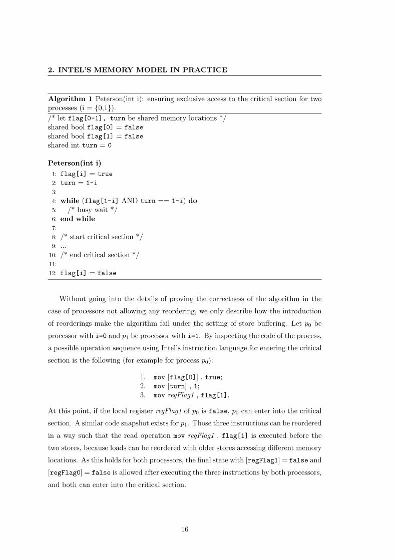
Algorithm 1 Peterson(int i): ensuring exclusive access to the critical section for twoprocesses (i = 0,1)./* let flag[0-1], turn be shared memory locations */shared bool flag[0] = false
shared bool flag[1] = false
shared int turn = 0
Peterson(int i)
1: flag[i] = true
2: turn = 1-i
3:
4: while (flag[1-i] AND turn == 1-i) do5: /* busy wait */6: end while7:
8: /* start critical section */9: ...
10: /* end critical section */11:
12: flag[i] = false
Without going into the details of proving the correctness of the algorithm in the
case of processors not allowing any reordering, we only describe how the introduction
of reorderings make the algorithm fail under the setting of store buffering. Let p0 be
processor with i=0 and p1 be processor with i=1. By inspecting the code of the process,
a possible operation sequence using Intel’s instruction language for entering the critical
section is the following (for example for process p0):
1. mov [flag[0]] , true;2. mov [turn] , 1;3. mov regFlag1 , flag[1].
At this point, if the local register regFlag1 of p0 is false, p0 can enter into the critical
section. A similar code snapshot exists for p1. Those three instructions can be reordered
in a way such that the read operation mov regFlag1 , flag[1] is executed before the
two stores, because loads can be reordered with older stores accessing different memory
locations. As this holds for both processors, the final state with [regFlag1] = false and
[regFlag0] = false is allowed after executing the three instructions by both processors,
and both can enter into the critical section.
16
2.4 Discussion
To conclude, if a programmer wants to ensure a mutual exclusion algorithm to be
correct on modern multi-core processors, he cannot naively use classic mutual exclu-
sion algorithms due to the reorderings allowed by these processors. However, one can
make these algorithms correct by using the already mentioned memory fence opera-
tions or lock instructions, but these must be used sparingly in order to not the loose
the performance gain that comes precisely from only implementing a relaxed memory
model.
2.4 Discussion
In this chapter, we have discussed the initial failure to provide good definitions of the
memory models of multi-core processors. Previously mentioned work on these defini-
tions has been developed in order to provide programmers, as well as researchers, with
a valid base to work with and reason about memory models, in the sense of providing
a well described abstract memory machine satisfying current informal processor defi-
nitions. Such an abstract memory machine does ignore other optimization techniques
such as pipelining, caches or speculative executions, because all those techniques are
not visible by any executed sequential code.
In summary, in a multi-threaded program, each program may have a tenuously
different view of the memory, due to the memory model implemented on the processor.
Such memory models are called weak, or relaxed, memory models, and are designed
only to speed up performance of concurrent programs, which makes complete sense
for totally independent tasks being allocated on different processor cores, but becomes
quite difficult to exploit correctly when interaction, for instance sharing some variables,
is needed.
In the next chapter, we will introduce the different memory models we will consider
in this thesis, as well as an associated concurrent system description language and its
memory operations.
17

Chapter 3
Memory Models and Concurrent
Systems
In the previous chapter, we have motivated the need for precise formal memory models.
In this chapter, we introduce the memory models that will be used in this thesis,
and that can all be found in the literature. For each memory model we consider,
there exists both an operational definition as well as an axiomatic definition. The
operational definition makes understanding the memory model very easy because it
is defined visually by different components and the relations between these. On the
other hand, the axiomatic definitions might give a better understanding of the exact
differences between the memory models, and also makes obvious the inclusion relations
existing between the executions allowed by the various models. As just defining a
memory model does not lead directly to a system one can work on and reason about,
we will introduce, for each memory model we use, a concurrent system description
language with its associated operations and semantics.
We will start in Section 3.1 by the strongest memory model, called sequential consis-
tency (SC), and which has traditionally been the reference for software designers when
parallel programs are developed. However, this memory model no longer corresponds
to what is implemented in processors, which only guarantee weak (or relaxed) memory
models. We will consider two relaxed memory models, both of which can be modeled
by the use of store buffers only. The first model we will consider is called Total Store
Order (TSO), Section 3.2, in which store operations can be buffered and postponed
globally after later loads, though these later loads can see all earlier locally buffered
19
3. MEMORY MODELS AND CONCURRENT SYSTEMS
stores. This can be modeled by the use of one store buffer per processor core, and is
consistent with the memory orderings possible on current Intel x86 processors. An even
more relaxed memory model is Partial Store Order (PSO), Section 3.3, which is weaker
than TSO since it additionally allows stores accessing different memory locations to
be reordered within the same processor core. This can be modeled by using a store
buffer per processor core and per memory location. It is worth mentioning that TSO
and PSO were both first introduced in the SPARC architecture manuals, version 8 [68]
and 9 [69]. Intel’s memory orderings are consistent with this definition of TSO, and
thus TSO was the starting point of the definition of x86-TSO [60, 65], Section 3.4,
introduced to model Intel’s x86 processors. x86-TSO is an extension of TSO adding
lock and synchronization operations to TSO in order to include these operations di-
rectly into the memory model, rather than considering them alongside the processor
memory model. Similar extensions can also be introduced for PSO with one additional
synchronization operation. Finally, Section 3.5 will discuss relations between memory
models and their extensions.
3.1 Sequential Consistency (SC)
The sequential consistency memory model is the most commonly known memory model,
and was introduced first by Lamport in [43]. Lamport introduced the notions of se-
quential processor and sequential multiprocessor. A processor is said to be sequential if
the following condition is satisfied:
The result of an execution is the same as if the operations had been executedin the order specified by the program.
Leslie Lamport, 1979, [43].
Then, a multiprocessor is called sequentially consistent if the following condition is
satisfied:
The result of any execution is the same as if the operations of all the pro-cessors were executed in some sequential order, and the operations of eachindividual processor appear in this sequence in the order specified by its pro-gram.
Leslie Lamport, 1979, [43].
20

3.1 Sequential Consistency (SC)
In other words, a multiprocessor is sequentially consistent if any possible execution
of a program on this multiprocessor corresponds to an interleaving of the individual
processors’ instructions, where the order of the instructions of each processor must be
the order of the instructions specified by the program.
Remark 3.1. When talking about reorderings, we talk about reorderings of instructions
that are only visible when looking at what happens in the memory and how this is viewed
by different processor cores of a multi-core processor, while each core of course only sees
the program order of the instructions it is executing. An instance of the execution of
a program on a processor is called process. Processes contain the instruction sequence
of the program, a program counter giving the location of the current instruction in the
program and other information relative to the execution of the program. The operating
system may distribute the different processes on one or more physical processor cores
(we will not enter into details of operating systems, schedulers etc). As reorderings
(not in SC but in TSO and PSO) are only possible with respect to processor cores
rather than processes, the most general case of distribution of the processes onto physical
processor cores is the one where each process is executed on a different core, which we
will consider to always be the case. For this reason, we allow ourselves to use processor
core, processor and processes interchangeably. When talking about a multiprocessor
or a multi-core processor, we mean the abstract memory machine (or abstract memory
system) that behaves like a multiprocessor sharing memory according to a given memory
model, for example an SC-machine or TSO-system.
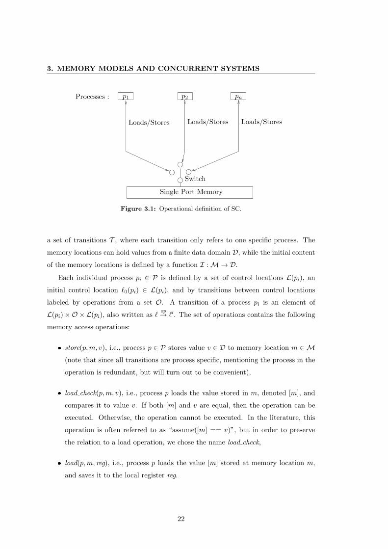
The operational definition of SC is given in Fig. 3.1. It consists of a set of processes
and a shared memory unit. Each process has a direct connection to the shared memory
unit, where each memory access has to be completed (i.e.,becomes visible globally)
before the process can continue its execution. Also note that the SC-machine can use the
switch to change nondeterministically the process that is connected with the memory
unit, a way to permit all possible interleavings of the instructions of all processes. Only
considering the memory access operations to compute all possible interleavings is safe
because only those operations have a global effect.
After giving the operational definition of SC, we will define the associated concurrent
system model with its operations and semantics. We chose a very natural model in
which there exists a counterpart of each component of the operational definition. An
SC concurrent system model is a tuple (P,M, T ), composed of a set of n processes
P = p1, p2, . . . , pn, a set of k shared memory locations M = m1,m2, . . . ,mk and
21
3. MEMORY MODELS AND CONCURRENT SYSTEMS
Switch
Single Port Memory
Loads/Stores
p2
Loads/Stores
pn
Loads/Stores
p1Processes :
Figure 3.1: Operational definition of SC.
a set of transitions T , where each transition only refers to one specific process. The
memory locations can hold values from a finite data domain D, while the initial content
of the memory locations is defined by a function I :M→D.
Each individual process pi ∈ P is defined by a set of control locations L(pi), an
initial control location `0(pi) ∈ L(pi), and by transitions between control locations
labeled by operations from a set O. A transition of a process pi is an element of
L(pi)×O ×L(pi), also written as `op→ `′. The set of operations contains the following
memory access operations:
store(p,m, v), i.e., process p ∈ P stores value v ∈ D to memory location m ∈ M
(note that since all transitions are process specific, mentioning the process in the
operation is redundant, but will turn out to be convenient),
load check(p,m, v), i.e., process p loads the value stored in m, denoted [m], and
compares it to value v. If both [m] and v are equal, then the operation can be
executed. Otherwise, the operation cannot be executed. In the literature, this
operation is often referred to as “assume([m] == v)”, but in order to preserve
the relation to a load operation, we chose the name load check,
load(p,m, reg), i.e., process p loads the value [m] stored at memory location m,
and saves it to the local register reg.
22
3.1 Sequential Consistency (SC)
The semantics of such a concurrent system model corresponding to SC is the usual
interleaving semantics in which all the possible behaviors are those that are interleavings
of the executions of the different processes. A global state is composed of a control
location for each process and a memory content for each memory location. The initial
state is composed of the initial control locations of the processes and by the initial
content of the memory locations. One can access each part of a global state by the
following functions: cp(s) accesses the control location of process p in s and m(s)
accesses the value stored at memory location m in s.
If each part of the system is restricted to be finite, there is a finite number of possible
global states. Let nb(L(pi)) be the number of control locations of process pi and let
nb(mi) be the number of values mi can take, then the maximum number of global
states is nb(L(p1)) × · · ·× nb(L(pn)) × nb(m1) × · · ·× nb(mk). This is an important
property of the type of programs we are going to handle within this thesis: we only
consider programs that are finite-state under SC. Future work could focus on adapting
our approach to programs that do consider infinite data domains.
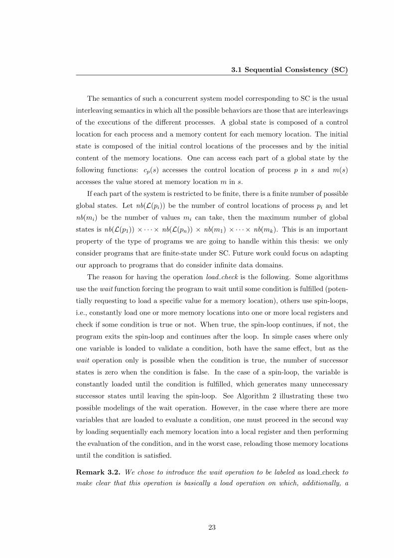
The reason for having the operation load check is the following. Some algorithms
use the wait function forcing the program to wait until some condition is fulfilled (poten-
tially requesting to load a specific value for a memory location), others use spin-loops,
i.e., constantly load one or more memory locations into one or more local registers and
check if some condition is true or not. When true, the spin-loop continues, if not, the
program exits the spin-loop and continues after the loop. In simple cases where only
one variable is loaded to validate a condition, both have the same effect, but as the
wait operation only is possible when the condition is true, the number of successor
states is zero when the condition is false. In the case of a spin-loop, the variable is
constantly loaded until the condition is fulfilled, which generates many unnecessary
successor states until leaving the spin-loop. See Algorithm 2 illustrating these two
possible modelings of the wait operation. However, in the case where there are more
variables that are loaded to evaluate a condition, one must proceed in the second way
by loading sequentially each memory location into a local register and then performing
the evaluation of the condition, and in the worst case, reloading those memory locations
until the condition is satisfied.
Remark 3.2. We chose to introduce the wait operation to be labeled as load check to
make clear that this operation is basically a load operation on which, additionally, a
23
3. MEMORY MODELS AND CONCURRENT SYSTEMS
Algorithm 2 Illustration of the two ways of modeling a wait operation.
/* let x be a shared memory location */
1: int x = 0
/* program code of process 1 using load check */
1: load check(p1, x, 1)
/* program code of process 2 using spin-loops */
1: int reg2: load(p2, x, reg)3: while (reg != 1) do4: load(p2, x, reg)5: end while
check verifying some condition is applied. In what follows, the load check and the load
operations are considered to be identical for what concerns the axiomatic definition of
memory ordering. Indeed, once a load operation becomes visible in the memory order,
a loaded value is associated to the load operation and is thus fixed. The operation thus
has the same effect as a load check operation for which the value that is checked for is
the same as the value read by the load. Of course, the value read by the load operation
is assigned to a local variable, while a load check does not assign any value to a local
register, but lets the process move to a state that keeps track of the information that the
load check was executed successfully with the current condition. For this reason, both
are equivalent.
We conclude the section by giving the axiomatic definition of SC, but first, we need
to introduce some notations. The axiomatic definitions use the concepts of program
order and memory order. The program order, also noted by <p, is a partial order in
which the instructions of each process are ordered as executed, but where instructions
of different processes are not ordered with respect to each other. The memory order,
noted by <m, is a total order over all memory accesses of all processes, representing
the order in which these operations become globally visible. By op we represent any
memory access operation (load1 or store.). Then, Definition 3.3 gives the axiomatic
definition of an SC-execution.
1As we said before, when referring to a load operation axiomatically, it can either be a load or aload check operation.
24
3.2 Total Store Order (TSO)
Definition 3.3. Let <p be the program order. An execution is an SC-execution if there
exists a memory order <m satisfying the following condition:
1. ∀opi, opj : opi <p opj ⇒ opi <m opj
2. The value read by a load operation on location a is the most recent value stored
to location a in memory order. If no store to location a occurs in memory order
before the load operation, the value read is the initial value of location a.
Thus, SC does not allow any instructions to be reordered, as the memory order has
to respect the program orders of the different processes, and each operation is visible
to all directly after being executed. A multiprocessor, or abstract memory machine,
implements SC if all possible executions are SC-executions.
3.2 Total Store Order (TSO)
The total store order (TSO) memory model is the one on which is based the x86-
TSO memory model (see section 3.4), which is consistent with the memory model
implemented on Intel’s x86 processors, and thus TSO covers an important fraction of
current multiprocessors. TSO defines the memory model with its possible reorderings,
whereas x86-TSO extends it with a new component, introducing additional operations
in order to be able to fully model processors, including locked and synchronization
instructions.
TSO was first introduced in [68, 69], which are versions 8 and 9 of “The SPARC
architecture manual”. In TSO, a processor can delay a store after a later load, which
improves performance. Indeed, waiting for each store to complete before continuing its
execution would significantly slow down the processor, since shared memory is much
slower than the processor itself. The possibility of delaying stores can be interpreted
in two ways: (1) stores can be reordered with later loads within the same processor,
or (2) stores can be buffered in a processor-local store buffer. Both interpretation are
equivalent (as has been proved in [65]), the first being expressed in axiomatic terms,
the second using operational notions.
We start by giving the operational definition of TSO, see Fig. 3.2. In TSO, each
process writes its store operations not directly into the shared memory, but adds them
25
3. MEMORY MODELS AND CONCURRENT SYSTEMS
Stores StoresLoads Loads Loads
Stores
Single Port Memory
Switch
Commits Commits Commits
store
p1 p2 pn
FIFO
buffer
Processes :
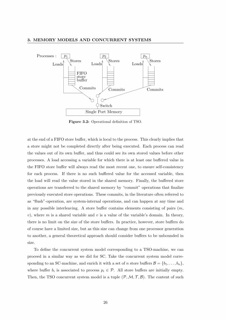
Figure 3.2: Operational definition of TSO.
at the end of a FIFO store buffer, which is local to the process. This clearly implies that
a store might not be completed directly after being executed. Each process can read
the values out of its own buffer, and thus could see its own stored values before other
processes. A load accessing a variable for which there is at least one buffered value in
the FIFO store buffer will always read the most recent one, to ensure self-consistency
for each process. If there is no such buffered value for the accessed variable, then
the load will read the value stored in the shared memory. Finally, the buffered store
operations are transferred to the shared memory by “commit” operations that finalize
previously executed store operations. These commits, in the literature often referred to
as “flush”-operation, are system-internal operations, and can happen at any time and
in any possible interleaving. A store buffer contains elements consisting of pairs (m,
v), where m is a shared variable and v is a value of the variable’s domain. In theory,
there is no limit on the size of the store buffers. In practice, however, store buffers do
of course have a limited size, but as this size can change from one processor generation
to another, a general theoretical approach should consider buffers to be unbounded in
size.
To define the concurrent system model corresponding to a TSO-machine, we can
proceed in a similar way as we did for SC. Take the concurrent system model corre-
sponding to an SC-machine, and enrich it with a set of n store buffers B = b1, . . . , bn,where buffer bi is associated to process pi ∈ P. All store buffers are initially empty.
Then, the TSO concurrent system model is a tuple (P,M, T ,B). The content of such
26
3.2 Total Store Order (TSO)
a store buffer can, as mentioned before, be seen as a word in (M×D)∗. Memory ac-
cess operations then need to be mapped to specific TSO-machine operations correctly
handling the store buffers.
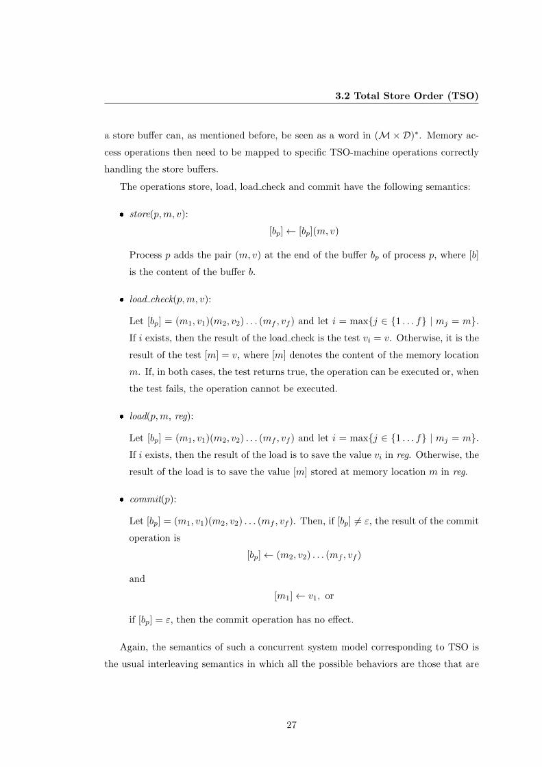
The operations store, load, load check and commit have the following semantics:
store(p,m, v):
[bp]← [bp](m, v)
Process p adds the pair (m, v) at the end of the buffer bp of process p, where [b]
is the content of the buffer b.
load check(p,m, v):
Let [bp] = (m1, v1)(m2, v2) . . . (mf , vf ) and let i = maxj ∈ 1 . . . f | mj = m.If i exists, then the result of the load check is the test vi = v. Otherwise, it is the
result of the test [m] = v, where [m] denotes the content of the memory location
m. If, in both cases, the test returns true, the operation can be executed or, when
the test fails, the operation cannot be executed.
load(p,m, reg):
Let [bp] = (m1, v1)(m2, v2) . . . (mf , vf ) and let i = maxj ∈ 1 . . . f | mj = m.If i exists, then the result of the load is to save the value vi in reg. Otherwise, the
result of the load is to save the value [m] stored at memory location m in reg.
commit(p):
Let [bp] = (m1, v1)(m2, v2) . . . (mf , vf ). Then, if [bp] 6= ε, the result of the commit
operation is
[bp]← (m2, v2) . . . (mf , vf )
and
[m1]← v1, or
if [bp] = ε, then the commit operation has no effect.
Again, the semantics of such a concurrent system model corresponding to TSO is
the usual interleaving semantics in which all the possible behaviors are those that are
27
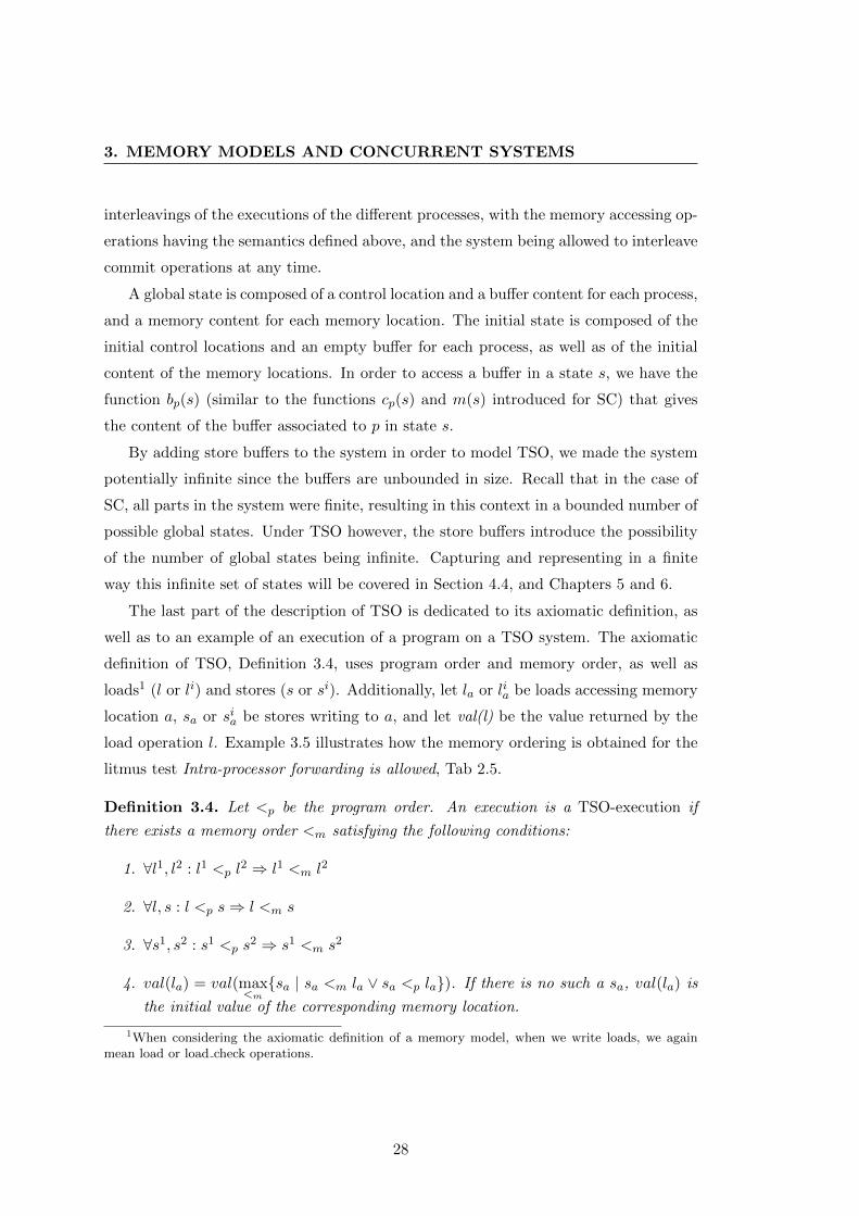
3. MEMORY MODELS AND CONCURRENT SYSTEMS
interleavings of the executions of the different processes, with the memory accessing op-
erations having the semantics defined above, and the system being allowed to interleave
commit operations at any time.
A global state is composed of a control location and a buffer content for each process,
and a memory content for each memory location. The initial state is composed of the
initial control locations and an empty buffer for each process, as well as of the initial
content of the memory locations. In order to access a buffer in a state s, we have the
function bp(s) (similar to the functions cp(s) and m(s) introduced for SC) that gives
the content of the buffer associated to p in state s.
By adding store buffers to the system in order to model TSO, we made the system
potentially infinite since the buffers are unbounded in size. Recall that in the case of
SC, all parts in the system were finite, resulting in this context in a bounded number of
possible global states. Under TSO however, the store buffers introduce the possibility
of the number of global states being infinite. Capturing and representing in a finite
way this infinite set of states will be covered in Section 4.4, and Chapters 5 and 6.
The last part of the description of TSO is dedicated to its axiomatic definition, as
well as to an example of an execution of a program on a TSO system. The axiomatic
definition of TSO, Definition 3.4, uses program order and memory order, as well as
loads1 (l or li) and stores (s or si). Additionally, let la or lia be loads accessing memory
location a, sa or sia be stores writing to a, and let val(l) be the value returned by the
load operation l. Example 3.5 illustrates how the memory ordering is obtained for the
litmus test Intra-processor forwarding is allowed, Tab 2.5.
Definition 3.4. Let <p be the program order. An execution is a TSO-execution if
there exists a memory order <m satisfying the following conditions:
1. ∀l1, l2 : l1 <p l2 ⇒ l1 <m l2
2. ∀l, s : l <p s⇒ l <m s
3. ∀s1, s2 : s1 <p s2 ⇒ s1 <m s2
4. val(la) = val(max<m
sa | sa <m la ∨ sa <p la). If there is no such a sa, val(la) is
the initial value of the corresponding memory location.
1When considering the axiomatic definition of a memory model, when we write loads, we againmean load or load check operations.
28
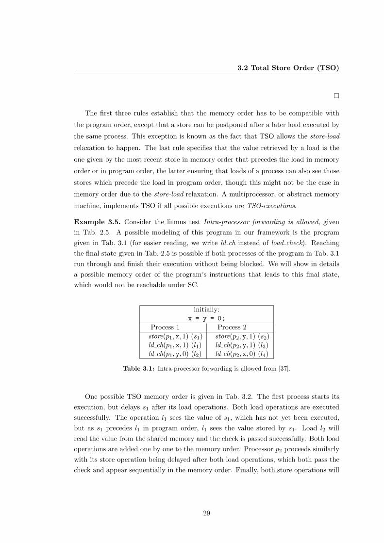
3.2 Total Store Order (TSO)
The first three rules establish that the memory order has to be compatible with
the program order, except that a store can be postponed after a later load executed by
the same process. This exception is known as the fact that TSO allows the store-load
relaxation to happen. The last rule specifies that the value retrieved by a load is the
one given by the most recent store in memory order that precedes the load in memory
order or in program order, the latter ensuring that loads of a process can also see those
stores which precede the load in program order, though this might not be the case in
memory order due to the store-load relaxation. A multiprocessor, or abstract memory
machine, implements TSO if all possible executions are TSO-executions.
Example 3.5. Consider the litmus test Intra-processor forwarding is allowed, given
in Tab. 2.5. A possible modeling of this program in our framework is the program
given in Tab. 3.1 (for easier reading, we write ld ch instead of load check). Reaching
the final state given in Tab. 2.5 is possible if both processes of the program in Tab. 3.1
run through and finish their execution without being blocked. We will show in details
a possible memory order of the program’s instructions that leads to this final state,
which would not be reachable under SC.
initially:x = y = 0;
Process 1 Process 2
store(p1, x, 1) (s1) store(p2, y, 1) (s2)ld ch(p1, x, 1) (l1) ld ch(p2, y, 1) (l3)ld ch(p1, y, 0) (l2) ld ch(p2, x, 0) (l4)
Table 3.1: Intra-processor forwarding is allowed from [37].
One possible TSO memory order is given in Tab. 3.2. The first process starts its
execution, but delays s1 after its load operations. Both load operations are executed
successfully. The operation l1 sees the value of s1, which has not yet been executed,
but as s1 precedes l1 in program order, l1 sees the value stored by s1. Load l2 will
read the value from the shared memory and the check is passed successfully. Both load
operations are added one by one to the memory order. Processor p2 proceeds similarly
with its store operation being delayed after both load operations, which both pass the
check and appear sequentially in the memory order. Finally, both store operations will
29
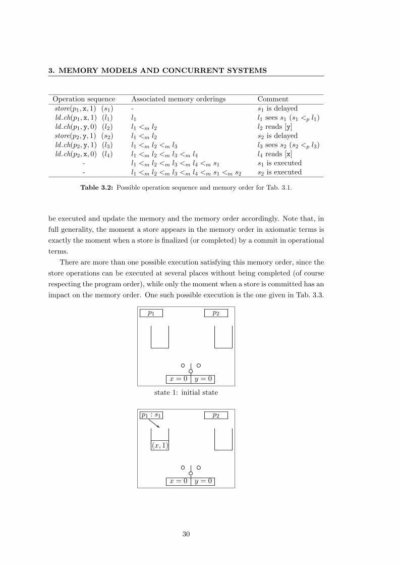
3. MEMORY MODELS AND CONCURRENT SYSTEMS
Operation sequence Associated memory orderings Comment
store(p1, x, 1) (s1) - s1 is delayedld ch(p1, x, 1) (l1) l1 l1 sees s1 (s1 <p l1)ld ch(p1, y, 0) (l2) l1 <m l2 l2 reads [y]store(p2, y, 1) (s2) l1 <m l2 s2 is delayedld ch(p2, y, 1) (l3) l1 <m l2 <m l3 l3 sees s2 (s2 <p l3)ld ch(p2, x, 0) (l4) l1 <m l2 <m l3 <m l4 l4 reads [x]
- l1 <m l2 <m l3 <m l4 <m s1 s1 is executed- l1 <m l2 <m l3 <m l4 <m s1 <m s2 s2 is executed
Table 3.2: Possible operation sequence and memory order for Tab. 3.1.
be executed and update the memory and the memory order accordingly. Note that, in
full generality, the moment a store appears in the memory order in axiomatic terms is
exactly the moment when a store is finalized (or completed) by a commit in operational
terms.
There are more than one possible execution satisfying this memory order, since the
store operations can be executed at several places without being completed (of course
respecting the program order), while only the moment when a store is committed has an
impact on the memory order. One such possible execution is the one given in Tab. 3.3.
x = 0 y = 0
p1 p2
state 1: initial state
x = 0 y = 0
p1 : s1 p2
(x, 1)
30
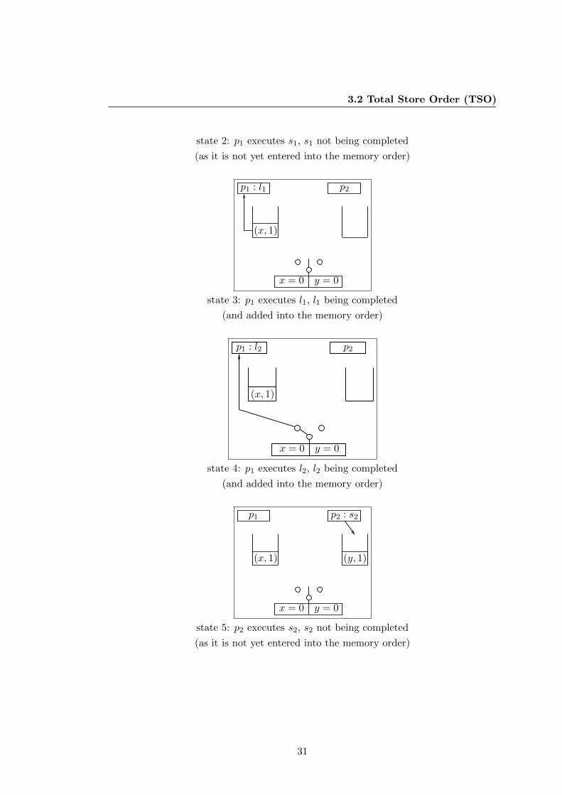
3.2 Total Store Order (TSO)
state 2: p1 executes s1, s1 not being completed
(as it is not yet entered into the memory order)
x = 0 y = 0
p1 : l1 p2
(x, 1)
state 3: p1 executes l1, l1 being completed
(and added into the memory order)
x = 0 y = 0
p1 : l2 p2
(x, 1)
state 4: p1 executes l2, l2 being completed
(and added into the memory order)
x = 0 y = 0
p1 p2 : s2
(x, 1) (y, 1)
state 5: p2 executes s2, s2 not being completed
(as it is not yet entered into the memory order)
31
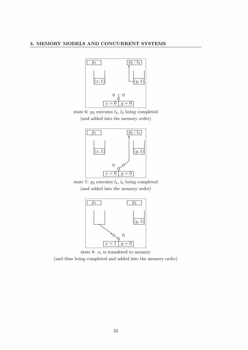
3. MEMORY MODELS AND CONCURRENT SYSTEMS
x = 0 y = 0
p1 p2 : l3
(x, 1) (y, 1)
state 6: p2 executes l3, l3 being completed
(and added into the memory order)
x = 0 y = 0
p1 p2 : l4
(x, 1) (y, 1)
state 7: p2 executes l4, l4 being completed
(and added into the memory order)
x = 1 y = 0
p1 p2
(y, 1)
state 8: s1 is transfered to memory
(and thus being completed and added into the memory order)
32
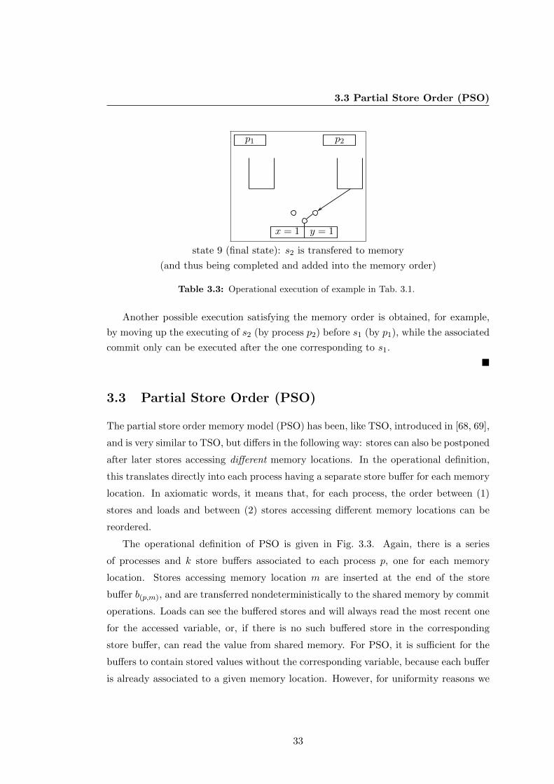
3.3 Partial Store Order (PSO)
x = 1 y = 1
p1 p2
state 9 (final state): s2 is transfered to memory
(and thus being completed and added into the memory order)
Table 3.3: Operational execution of example in Tab. 3.1.
Another possible execution satisfying the memory order is obtained, for example,
by moving up the executing of s2 (by process p2) before s1 (by p1), while the associated
commit only can be executed after the one corresponding to s1.
3.3 Partial Store Order (PSO)
The partial store order memory model (PSO) has been, like TSO, introduced in [68, 69],
and is very similar to TSO, but differs in the following way: stores can also be postponed
after later stores accessing different memory locations. In the operational definition,
this translates directly into each process having a separate store buffer for each memory
location. In axiomatic words, it means that, for each process, the order between (1)
stores and loads and between (2) stores accessing different memory locations can be
reordered.
The operational definition of PSO is given in Fig. 3.3. Again, there is a series
of processes and k store buffers associated to each process p, one for each memory
location. Stores accessing memory location m are inserted at the end of the store
buffer b(p,m), and are transferred nondeterministically to the shared memory by commit
operations. Loads can see the buffered stores and will always read the most recent one
for the accessed variable, or, if there is no such buffered store in the corresponding
store buffer, can read the value from shared memory. For PSO, it is sufficient for the
buffers to contain stored values without the corresponding variable, because each buffer
is already associated to a given memory location. However, for uniformity reasons we
33
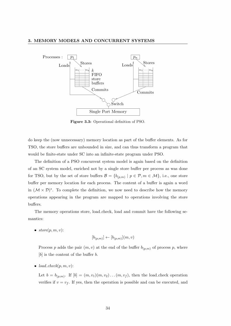
3. MEMORY MODELS AND CONCURRENT SYSTEMS
Switch
Single Port Memory
LoadsLoads
Commits
Stores Stores
Commits
p1 pn
m1 mk· · · · · ·m1 mk
FIFOstorebuffers
k
Processes :
Figure 3.3: Operational definition of PSO.
do keep the (now unnecessary) memory location as part of the buffer elements. As for
TSO, the store buffers are unbounded in size, and can thus transform a program that
would be finite-state under SC into an infinite-state program under PSO.
The definition of a PSO concurrent system model is again based on the definition
of an SC system model, enriched not by a single store buffer per process as was done
for TSO, but by the set of store buffers B = b(p,m) | p ∈ P,m ∈ M, i.e., one store
buffer per memory location for each process. The content of a buffer is again a word
in (M×D)∗. To complete the definition, we now need to describe how the memory
operations appearing in the program are mapped to operations involving the store
buffers.
The memory operations store, load check, load and commit have the following se-
mantics:
store(p,m, v):
[b(p,m)]← [b(p,m)](m, v)
Process p adds the pair (m, v) at the end of the buffer b(p,m) of process p, where
[b] is the content of the buffer b.
load check(p,m, v):
Let b = b(p,m). If [b] = (m, v1)(m, v2) . . . (m, vf ), then the load check operation
verifies if v = vf . If yes, then the operation is possible and can be executed, and
34
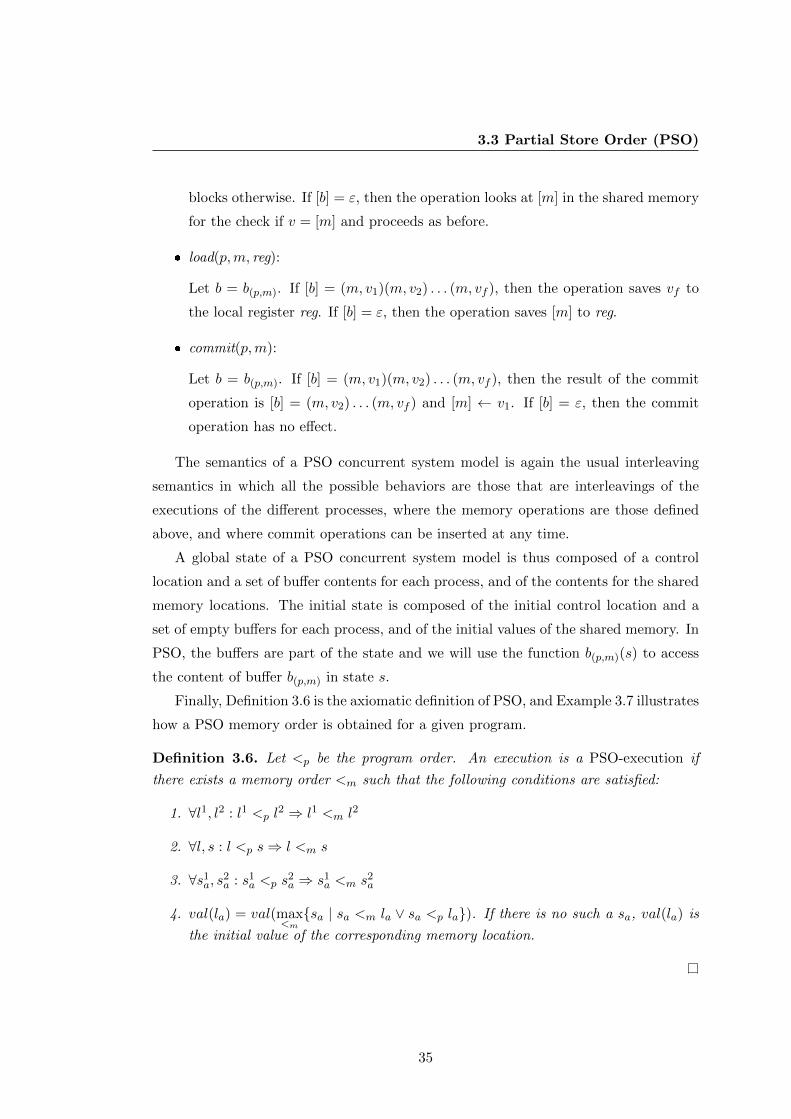
3.3 Partial Store Order (PSO)
blocks otherwise. If [b] = ε, then the operation looks at [m] in the shared memory
for the check if v = [m] and proceeds as before.
load(p,m, reg):
Let b = b(p,m). If [b] = (m, v1)(m, v2) . . . (m, vf ), then the operation saves vf to
the local register reg. If [b] = ε, then the operation saves [m] to reg.
commit(p,m):
Let b = b(p,m). If [b] = (m, v1)(m, v2) . . . (m, vf ), then the result of the commit
operation is [b] = (m, v2) . . . (m, vf ) and [m] ← v1. If [b] = ε, then the commit
operation has no effect.
The semantics of a PSO concurrent system model is again the usual interleaving
semantics in which all the possible behaviors are those that are interleavings of the
executions of the different processes, where the memory operations are those defined
above, and where commit operations can be inserted at any time.
A global state of a PSO concurrent system model is thus composed of a control
location and a set of buffer contents for each process, and of the contents for the shared
memory locations. The initial state is composed of the initial control location and a
set of empty buffers for each process, and of the initial values of the shared memory. In
PSO, the buffers are part of the state and we will use the function b(p,m)(s) to access
the content of buffer b(p,m) in state s.
Finally, Definition 3.6 is the axiomatic definition of PSO, and Example 3.7 illustrates
how a PSO memory order is obtained for a given program.
Definition 3.6. Let <p be the program order. An execution is a PSO-execution if
there exists a memory order <m such that the following conditions are satisfied:
1. ∀l1, l2 : l1 <p l2 ⇒ l1 <m l2
2. ∀l, s : l <p s⇒ l <m s
3. ∀s1a, s2a : s1a <p s2a ⇒ s1a <m s2a
4. val(la) = val(max<m
sa | sa <m la ∨ sa <p la). If there is no such a sa, val(la) is
the initial value of the corresponding memory location.
35
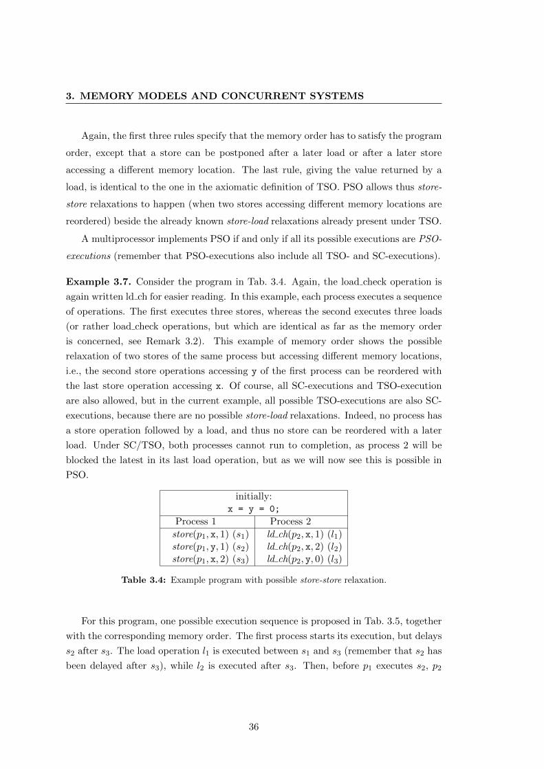
3. MEMORY MODELS AND CONCURRENT SYSTEMS
Again, the first three rules specify that the memory order has to satisfy the program
order, except that a store can be postponed after a later load or after a later store
accessing a different memory location. The last rule, giving the value returned by a
load, is identical to the one in the axiomatic definition of TSO. PSO allows thus store-
store relaxations to happen (when two stores accessing different memory locations are
reordered) beside the already known store-load relaxations already present under TSO.
A multiprocessor implements PSO if and only if all its possible executions are PSO-
executions (remember that PSO-executions also include all TSO- and SC-executions).
Example 3.7. Consider the program in Tab. 3.4. Again, the load check operation is
again written ld ch for easier reading. In this example, each process executes a sequence
of operations. The first executes three stores, whereas the second executes three loads
(or rather load check operations, but which are identical as far as the memory order
is concerned, see Remark 3.2). This example of memory order shows the possible
relaxation of two stores of the same process but accessing different memory locations,
i.e., the second store operations accessing y of the first process can be reordered with
the last store operation accessing x. Of course, all SC-executions and TSO-execution
are also allowed, but in the current example, all possible TSO-executions are also SC-
executions, because there are no possible store-load relaxations. Indeed, no process has
a store operation followed by a load, and thus no store can be reordered with a later
load. Under SC/TSO, both processes cannot run to completion, as process 2 will be
blocked the latest in its last load operation, but as we will now see this is possible in
PSO.
initially:x = y = 0;
Process 1 Process 2
store(p1, x, 1) (s1) ld ch(p2, x, 1) (l1)store(p1, y, 1) (s2) ld ch(p2, x, 2) (l2)store(p1, x, 2) (s3) ld ch(p2, y, 0) (l3)
Table 3.4: Example program with possible store-store relaxation.
For this program, one possible execution sequence is proposed in Tab. 3.5, together
with the corresponding memory order. The first process starts its execution, but delays
s2 after s3. The load operation l1 is executed between s1 and s3 (remember that s2 has
been delayed after s3), while l2 is executed after s3. Then, before p1 executes s2, p2
36
3.4 Extensions with Locks and Memory Fences
executed l3 and finishes its execution. Finally, p0 executes s2 and finishes its execution
as well.
Operation sequence Associated memory orderings Comment
store(p1, x, 1) (s1) s1 s1 is executedld ch(p2, x, 1) (l1) s1 <m l1 l1 sees s1store(p1, y, 1) (s2) s1 <m l1 s2 is delayedstore(p1, x, 2) (s3) s1 <m l1 <m s3 s3 is executedld ch(p2, x, 2) (l2) s1 <m l1 <m s3 <m l2 l2 sees s3ld ch(p2, y, 0) (l3) s1 <m l1 <m s3 <m l2 <m l3 l3 reads [y]
- s1 <m l1 <m s3 <m l2 <m l3 <m s2 s2 is executed
Table 3.5: Possible operation sequence and memory order for Tab. 3.4.
3.4 Extensions with Locks and Memory Fences
In this section, we will present the extensions of TSO and PSO mentioned above. The
TSO extension, x86-TSO, has been defined in [60, 65].
The PSO extension has not yet been defined formally, but is an easy adaptation of
the TSO extension. Indeed, such an extension has already been used in [41] but, in
this work no difference was made between the fences needed to respectively limit TSO
and PSO relations.
3.4.1 Extended TSO: x86-TSO
Real processors do not only define rules for potential reorderings, but also propose syn-
chronization and locking primitives. The synchronization instruction under TSO, often
called mfence, can be used to prevent a store-load relaxation from happening between
store operations occurring before and load operations occurring after the mfence. In
axiomatic terms, this means that if there is an mfence between a store and a later load,
these cannot be reordered, and the store has to complete before the load is executed.
Thus, the most meaningful place for an mfence is to be inserted between a store and a
subsequent load. In terms of the operational definition, this means that all previously
buffered stores must be transferred to the shared memory before the mfence operation
can be executed.
37
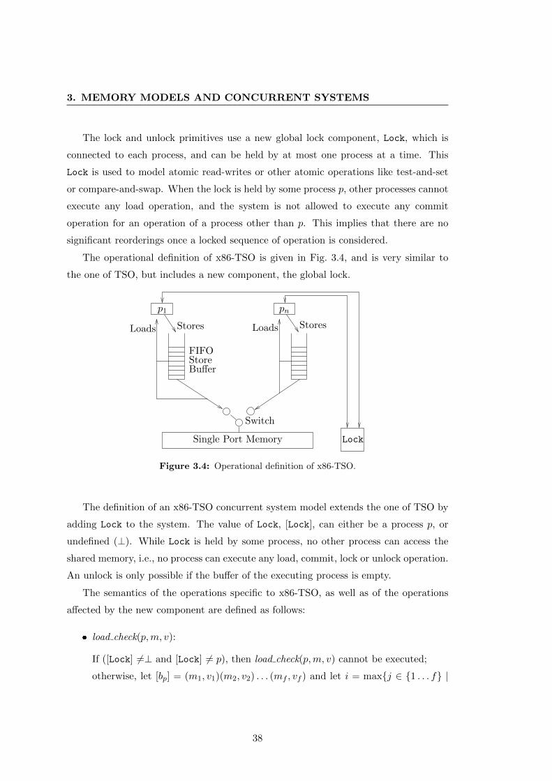
3. MEMORY MODELS AND CONCURRENT SYSTEMS
The lock and unlock primitives use a new global lock component, Lock, which is
connected to each process, and can be held by at most one process at a time. This
Lock is used to model atomic read-writes or other atomic operations like test-and-set
or compare-and-swap. When the lock is held by some process p, other processes cannot
execute any load operation, and the system is not allowed to execute any commit
operation for an operation of a process other than p. This implies that there are no
significant reorderings once a locked sequence of operation is considered.
The operational definition of x86-TSO is given in Fig. 3.4, and is very similar to
the one of TSO, but includes a new component, the global lock.
Switch
Single Port Memory
Loads
StoreFIFO
p1
Buffer
Loads
pn
StoresStores
Lock
Figure 3.4: Operational definition of x86-TSO.
The definition of an x86-TSO concurrent system model extends the one of TSO by
adding Lock to the system. The value of Lock, [Lock], can either be a process p, or
undefined (⊥). While Lock is held by some process, no other process can access the
shared memory, i.e., no process can execute any load, commit, lock or unlock operation.
An unlock is only possible if the buffer of the executing process is empty.
The semantics of the operations specific to x86-TSO, as well as of the operations
affected by the new component are defined as follows:
load check(p,m, v):
If ([Lock] 6=⊥ and [Lock] 6= p), then load check(p,m, v) cannot be executed;
otherwise, let [bp] = (m1, v1)(m2, v2) . . . (mf , vf ) and let i = maxj ∈ 1 . . . f |
38
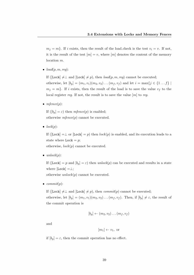
3.4 Extensions with Locks and Memory Fences
mj = m. If i exists, then the result of the load check is the test vi = v. If not,
it is the result of the test [m] = v, where [m] denotes the content of the memory
location m.
load(p,m, reg):
If ([Lock] 6=⊥ and [Lock] 6= p), then load(p,m, reg) cannot be executed;
otherwise, let [bp] = (m1, v1)(m2, v2) . . . (mf , vf ) and let i = maxj ∈ 1 . . . f |mj = m. If i exists, then the result of the load is to save the value vf to the
local register reg. If not, the result is to save the value [m] to reg.
mfence(p):
If ([bp] = ε) then mfence(p) is enabled;
otherwise mfence(p) cannot be executed.
lock(p):
If ([Lock] =⊥ or [Lock] = p) then lock(p) is enabled, and its execution leads to a
state where Lock = p;
otherwise, lock(p) cannot be executed.
unlock(p):
If ([Lock] = p and [bp] = ε) then unlock(p) can be executed and results in a state
where [Lock] =⊥;
otherwise unlock(p) cannot be executed.
commit(p):
If ([Lock] 6=⊥ and [Lock] 6= p), then commit(p) cannot be executed;
otherwise, let [bp] = (m1, v1)(m2, v2) . . . (mf , vf ). Then, if [bp] 6= ε, the result of
the commit operation is
[bp]← (m2, v2) . . . (mf , vf )
and
[m1]← v1, or
if [bp] = ε, then the commit operation has no effect.
39

3. MEMORY MODELS AND CONCURRENT SYSTEMS
The semantics of a x86-TSO concurrent system model is again the classical inter-
leaving semantics, where the memory operations are those defined above.
A global state of an x86-TSO concurrent system model is composed of all elements
already present in TSO, extended by the value of the global lock, which can be either
a process p or undefined (⊥) if no process holds the lock in the state. The initial state
extends the initial state of a TSO system by the initial value of the lock, ⊥. The value
of the global lock in state s can be accessed by the function Lock(s).
To conclude, we extend the axiomatic definition of TSO to x86-TSO, by adding
axiomatic rules for the new operations, where op is either a load or a store, l is a
load, M is an mfence, L is a lock and U is an unlock operation. An execution is an
x86-TSO-execution if there exists a memory order <m satisfying the 4 conditions of a
TSO-execution, as well as the following ones:
5. ∀ L, U, M, op: L, U, M <p L, U, M, op ⇒ L, U, M <m L, U, M, op
6. ∀ U, M, op: op <p U, M ⇒ op <m U, M
7. ∀ L, l: l <p L ⇒ l <m L
Those rules express the fact that none of the new operations can be reordered with
any other operation of the system, except that a store that precedes a lock may be
postponed after the lock, while an earlier load cannot be reordered with a later lock.
This corresponds perfectly with the semantics of the operational definition.
3.4.2 Extended PSO
As in the case of TSO, PSO does not fully represent the behavior of a PSO memory
machine, since it lacks the synchronization and lock operations. We will now intro-
duce extended-PSO, which is to PSO what x86-TSO is to TSO, but has not yet been
made explicit in the literature. Just as in x86-TSO, there is a global lock component
that completes the operational definition. As we saw in Section 3.3, PSO allows two
relaxations to occur, the store-load relaxation as well as the store-store relaxation for
stores accessing different memory locations. Thus, in PSO, we have not one but two
different fence operations. The first one, the mfence, is the same as in TSO and can
be used to disable store-load relaxations by blocking the process executing it until all
its buffers are empty. The second one is called sfence, and is used to disable store-store
40
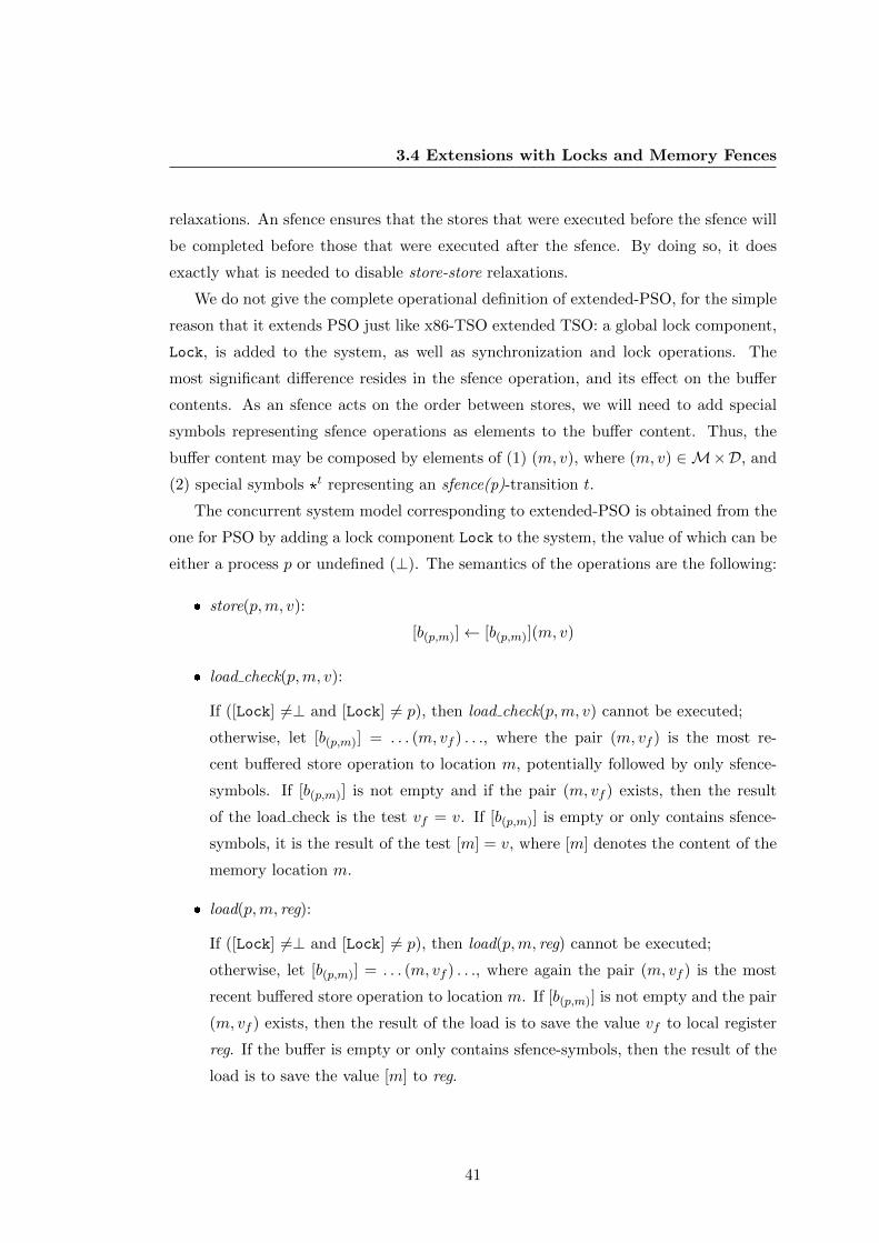
3.4 Extensions with Locks and Memory Fences
relaxations. An sfence ensures that the stores that were executed before the sfence will
be completed before those that were executed after the sfence. By doing so, it does
exactly what is needed to disable store-store relaxations.
We do not give the complete operational definition of extended-PSO, for the simple
reason that it extends PSO just like x86-TSO extended TSO: a global lock component,
Lock, is added to the system, as well as synchronization and lock operations. The
most significant difference resides in the sfence operation, and its effect on the buffer
contents. As an sfence acts on the order between stores, we will need to add special
symbols representing sfence operations as elements to the buffer content. Thus, the
buffer content may be composed by elements of (1) (m, v), where (m, v) ∈M×D, and
(2) special symbols bt representing an sfence(p)-transition t.
The concurrent system model corresponding to extended-PSO is obtained from the
one for PSO by adding a lock component Lock to the system, the value of which can be
either a process p or undefined (⊥). The semantics of the operations are the following:
store(p,m, v):
[b(p,m)]← [b(p,m)](m, v)
load check(p,m, v):
If ([Lock] 6=⊥ and [Lock] 6= p), then load check(p,m, v) cannot be executed;
otherwise, let [b(p,m)] = . . . (m, vf ) . . ., where the pair (m, vf ) is the most re-
cent buffered store operation to location m, potentially followed by only sfence-
symbols. If [b(p,m)] is not empty and if the pair (m, vf ) exists, then the result
of the load check is the test vf = v. If [b(p,m)] is empty or only contains sfence-
symbols, it is the result of the test [m] = v, where [m] denotes the content of the
memory location m.
load(p,m, reg):
If ([Lock] 6=⊥ and [Lock] 6= p), then load(p,m, reg) cannot be executed;
otherwise, let [b(p,m)] = . . . (m, vf ) . . ., where again the pair (m, vf ) is the most
recent buffered store operation to location m. If [b(p,m)] is not empty and the pair
(m, vf ) exists, then the result of the load is to save the value vf to local register
reg. If the buffer is empty or only contains sfence-symbols, then the result of the
load is to save the value [m] to reg.
41
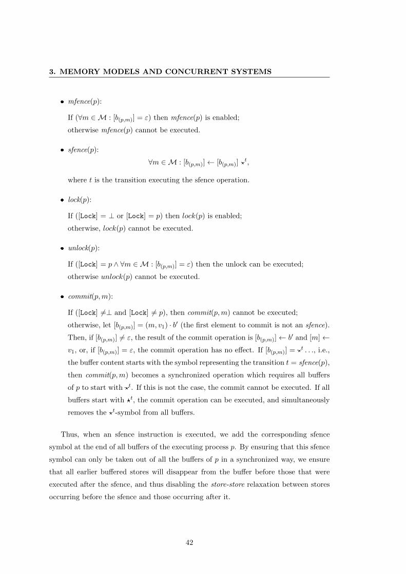
3. MEMORY MODELS AND CONCURRENT SYSTEMS
mfence(p):
If (∀m ∈M : [b(p,m)] = ε) then mfence(p) is enabled;
otherwise mfence(p) cannot be executed.
sfence(p):
∀m ∈M : [b(p,m)]← [b(p,m)] bt,
where t is the transition executing the sfence operation.
lock(p):
If ([Lock] = ⊥ or [Lock] = p) then lock(p) is enabled;
otherwise, lock(p) cannot be executed.
unlock(p):
If ([Lock] = p ∧ ∀m ∈M : [b(p,m)] = ε) then the unlock can be executed;
otherwise unlock(p) cannot be executed.
commit(p,m):
If ([Lock] 6=⊥ and [Lock] 6= p), then commit(p,m) cannot be executed;
otherwise, let [b(p,m)] = (m, v1) · b′ (the first element to commit is not an sfence).
Then, if [b(p,m)] 6= ε, the result of the commit operation is [b(p,m)]← b′ and [m]←v1, or, if [b(p,m)] = ε, the commit operation has no effect. If [b(p,m)] = bt . . ., i.e.,
the buffer content starts with the symbol representing the transition t = sfence(p),
then commit(p,m) becomes a synchronized operation which requires all buffers
of p to start with bt. If this is not the case, the commit cannot be executed. If all
buffers start with bt, the commit operation can be executed, and simultaneously
removes the bt-symbol from all buffers.
Thus, when an sfence instruction is executed, we add the corresponding sfence
symbol at the end of all buffers of the executing process p. By ensuring that this sfence
symbol can only be taken out of all the buffers of p in a synchronized way, we ensure
that all earlier buffered stores will disappear from the buffer before those that were
executed after the sfence, and thus disabling the store-store relaxation between stores
occurring before the sfence and those occurring after it.
42
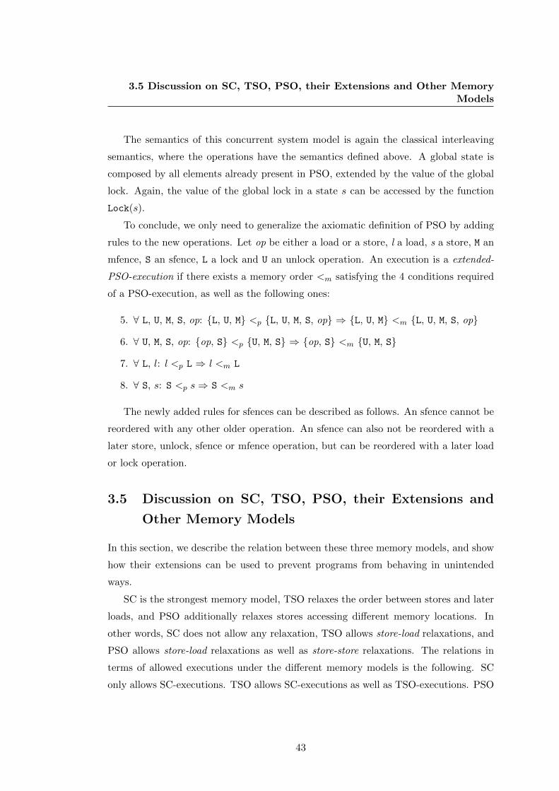
3.5 Discussion on SC, TSO, PSO, their Extensions and Other MemoryModels
The semantics of this concurrent system model is again the classical interleaving
semantics, where the operations have the semantics defined above. A global state is
composed by all elements already present in PSO, extended by the value of the global
lock. Again, the value of the global lock in a state s can be accessed by the function
Lock(s).
To conclude, we only need to generalize the axiomatic definition of PSO by adding
rules to the new operations. Let op be either a load or a store, l a load, s a store, M an
mfence, S an sfence, L a lock and U an unlock operation. An execution is a extended-
PSO-execution if there exists a memory order <m satisfying the 4 conditions required
of a PSO-execution, as well as the following ones:
5. ∀ L, U, M, S, op: L, U, M <p L, U, M, S, op ⇒ L, U, M <m L, U, M, S, op
6. ∀ U, M, S, op: op, S <p U, M, S ⇒ op, S <m U, M, S
7. ∀ L, l: l <p L ⇒ l <m L
8. ∀ S, s: S <p s⇒ S <m s
The newly added rules for sfences can be described as follows. An sfence cannot be
reordered with any other older operation. An sfence can also not be reordered with a
later store, unlock, sfence or mfence operation, but can be reordered with a later load
or lock operation.
3.5 Discussion on SC, TSO, PSO, their Extensions and
Other Memory Models
In this section, we describe the relation between these three memory models, and show
how their extensions can be used to prevent programs from behaving in unintended
ways.
SC is the strongest memory model, TSO relaxes the order between stores and later
loads, and PSO additionally relaxes stores accessing different memory locations. In
other words, SC does not allow any relaxation, TSO allows store-load relaxations, and
PSO allows store-load relaxations as well as store-store relaxations. The relations in
terms of allowed executions under the different memory models is the following. SC
only allows SC-executions. TSO allows SC-executions as well as TSO-executions. PSO
43
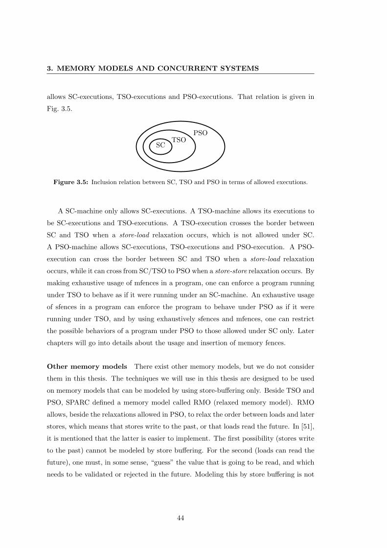
3. MEMORY MODELS AND CONCURRENT SYSTEMS
allows SC-executions, TSO-executions and PSO-executions. That relation is given in
Fig. 3.5.
SCTSO
PSO
Figure 3.5: Inclusion relation between SC, TSO and PSO in terms of allowed executions.
A SC-machine only allows SC-executions. A TSO-machine allows its executions to
be SC-executions and TSO-executions. A TSO-execution crosses the border between
SC and TSO when a store-load relaxation occurs, which is not allowed under SC.
A PSO-machine allows SC-executions, TSO-executions and PSO-execution. A PSO-
execution can cross the border between SC and TSO when a store-load relaxation
occurs, while it can cross from SC/TSO to PSO when a store-store relaxation occurs. By
making exhaustive usage of mfences in a program, one can enforce a program running
under TSO to behave as if it were running under an SC-machine. An exhaustive usage
of sfences in a program can enforce the program to behave under PSO as if it were
running under TSO, and by using exhaustively sfences and mfences, one can restrict
the possible behaviors of a program under PSO to those allowed under SC only. Later
chapters will go into details about the usage and insertion of memory fences.
Other memory models There exist other memory models, but we do not consider
them in this thesis. The techniques we will use in this thesis are designed to be used
on memory models that can be modeled by using store-buffering only. Beside TSO and
PSO, SPARC defined a memory model called RMO (relaxed memory model). RMO
allows, beside the relaxations allowed in PSO, to relax the order between loads and later
stores, which means that stores write to the past, or that loads read the future. In [51],
it is mentioned that the latter is easier to implement. The first possibility (stores write
to the past) cannot be modeled by store buffering. For the second (loads can read the
future), one must, in some sense, “guess” the value that is going to be read, and which
needs to be validated or rejected in the future. Modeling this by store buffering is not
44
3.5 Discussion on SC, TSO, PSO, their Extensions and Other MemoryModels
impossible, but would substantially complicate the “enumeration” of executions. An
execution that contains a load (thus “every” interesting execution) would need to guess
the value to be loaded. This guessing can be modeled by creating one execution for
each possible value to be loaded. Since each such speculative read must be validated at
some point in the future, some of the executions that were constructed will be rejected.
However, one does not exactly know when this rejecting might happen, and the number
of executions to enumerate quickly grows before one knows which execution to reject.
The techniques presented in this thesis strongly depend on analyzing the executions,
and a number of executions that is too large would make our techniques unusable in
practice. However, our techniques might help the programmer even in the case of RMO.
Indeed, as RMO is an extension to PSO (extension in the sense that all PSO-execution
will also be allowed by a RMO-machine), one could first analyze and potentially correct
a program under PSO in order to get a program in which one only needs to care about
load-store relaxations (those that are not allowed under PSO).
Another family of processors is IBM’s POWER multiprocessors. Those processors
do also allow reorderings that cannot be modeled only with store buffering, which
pushes thus this memory model out of the scope of our techniques.
There are still more memory models, but as we only handle SC, TSO and PSO in
this thesis, we will not review them exhaustively. The interested reader can refer to
[53, 54], or [12] (more theoretical work on memory models defining the barrier between
decidability and undecidability of state reachability of store-buffer based memory mod-
els) and [67] (Alpha processor), and others to get more information on other memory
models.
45

Chapter 4
Ingredients to our Approach
This chapter introduces basic information on the verification of programs and presents
techniques for dealing with underlying issues, such as the state-space explosion problem
or infinite state spaces.
Section 4.1 introduces the verification of concurrent programs, starting with basic
notions and followed by techniques used for this purpose. We describe what kind
of properties can be verified, and which are the drawbacks of the naive use of these
techniques when it comes down to the verification of real-life concurrent programs.
To tackle these drawbacks, Section 4.2 describes the partial-order reduction tech-
niques (POR). These techniques exploit independence of instructions of the program
in order to reduce the number of executions (or interleavings) to analyze, while still
being able to correctly verify the program with respect to a given property. Section 4.3
describes a technique that is very close to the main technique that is proposed in this
thesis. Our technique was clearly inspired by this one, but proceeds differently, and
includes partial-order reductions.
Finally, Section 4.4 introduces a data structure that allows the symbolic represen-
tation of potentially infinite sets of words. In our approach, the words will correspond
to the buffer contents that are necessary to model TSO/PSO.
4.1 Verification of Programs
Software verification is intended to be part of the design process of a program, and is
used to guarantee that a program satisfies its required properties.
47
4. INGREDIENTS TO OUR APPROACH
In this thesis, we only consider programs (or systems) that are composed of a finite
number of processes, which are communicating through a shared and finite memory
holding values from a finite memory domain. Those systems are called concurrent sys-
tems, and have already been defined in Chapter 3. Such concurrent systems are most of
the time hard to design, because the number of possible interleavings of the instructions
of the processes quickly becomes very large, even for simple systems. However, as pro-
cessors are ever more present in everyday life, especially in safety-critical environments
such as airplanes, trains or cars, it is very important to have techniques allowing the
verification of concurrent systems running on the now ubiquitous multi-core processors.
One of the existing techniques for the verification of concurrent systems with respect
to a given property is to generate all possible behaviors of the program and check that
they are compatible with the property. All possible behaviors can be obtained by
constructing and exploring the global state space. Checking a property while exploring
the state space is referred to as model-checking. For example, a property to verify might
be that some global state s is reachable. The model-checking procedure would explore
the state space, until either all global states have been visited but s was not reached,
or s is reached and the process is stopped.
To explore the global state space, one starts from the initial state and recursively
explores all successors of the states that are reached, following all enabled transitions.
If the state space is finite, it can be entirely explored. If it is infinite, there are three
possibilities. The first is to explore only a subset of the whole state space, introducing
for example a bound on the depth of the analyzed paths, and thus limiting oneself
to an under-approximation of the state space. The second one is to use abstraction
techniques to group sets into a finite number of classes, hence falling back to the finite-
state case, but loosing precision. Indeed, this over-approximates the state-space since
reachable and unreachable states might be grouped into the same class that will be
considered to be reachable and thus false negatives might occur. The last possibility is
to study the cause of the infinite nature of the state space and to use a symbolic data
structure that can finitely represent infinite sets of states, often at the cost of loosing
any guarantee of termination. This last option is the one used in this thesis.
The properties associated to a program are most of the time one of the following:
absence of deadlocks, absence of “bad states” represented by a safety property, or a
liveness property ensuring that something good will inevitably happen.
48
4.1 Verification of Programs
The advantage of model-checking is that it is fully automatic. After providing a
model of the system and a property to check, the model-checker explores the state
space while checking if the property is satisfied or violated. In case of a violated safety
property, the model-checker will visit a global state that does not satisfy the property,
and a trace, i.e.,an execution, leading to that state can often be provided. The user of
the model-checking procedure can then see why the property has been violated, and
can either correct the program, or refine the property.
The main drawback of state-space exploration, known as the state-space explosion
problem, is clearly the size of the state space, which is potentially exponential in the size
of the system model. In order to tackle this problem, partial-order reduction techniques
have been proposed to limit the number of interleavings to be checked, while preserving
the possibility of checking the property, see Section 4.2.
There exists two basic strategies for computing the state space of a concurrent
system: Depth-first search (DFS) and breadth-first search (BFS). In this thesis, we only
consider the first option, see Algorithm 3 and 4. During the search, a data structure
(often a hash table) stores all states that have been explored, in order to avoid re-
exploring the same state twice. In DFS, a LIFO stack is updated so that it always
contains the path to the current state. For a given state, DFS proceeds by exploring
recursively all successors that have not already been visited, and the exploration goes as
deep as possible in one direction, before backing up and continuing as deep as possible
in the next direction. BFS, on the other hand, works by using a FIFO stack of states
to be explored. For a given state, all of its successors that have not already been
visited are put on top of the FIFO stack. Then the algorithm continues by popping
the oldest state from the bottom of the stack and continues its exploration, and states
are explored in increasing level of depth.
Algorithm 3 Initialization and first call of depth-first search.
1: init(Stack) /* working states */2: init(H) /* Table of visited states */3: s0 = initial state4: push s0 onto Stack /* put initial state on stack */5: DFS() /* call recursive DFS algorithm */
Algorithm 3 first initializes the stack, the hash table and the initial state, and then
calls DFS() after putting the initial state onto the stack. The recursive procedure DFS()
49
4. INGREDIENTS TO OUR APPROACH
Procedure 4 DFS(): Basic depth-first search procedure.
1: s = peek(Stack)2: if (H does not contain s) then3: insert s in H4: T = enabled(s)5: for all t in T do6: s′ = succ(s, t)7: push s′ onto Stack8: DFS()9: end for
10: end if11: pop(Stack)
in Procedure 4 peeks1 at the state on top of the stack, state s. If s already has been
visited, the state is popped from the stack and the current search direction is stopped
and the algorithm backtracks to the predecessor state. If s consists in a new state, s
is inserted in the hash table, and the enabled transitions from s are assembled (i.e.,the
transition that are possible to be executed from state s) in set T . For all transitions t
in T , one by one, the successor s′ of s by executing t is computed by the function s′
= succ(s, t), put onto the stack and explored by a DFS() call. When the function call
returns, all successors of s′ have been visited, and the search continues with the next
transition of T . Once all transitions have been executed, the state s is popped from the
stack, and the function call returns to the caller, with all successors of s having been
explored and being present in the hash table.
4.2 Partial-Order Reduction
This section is giving an overview of the state-space reduction techniques described in
[31]. In that work, it has been shown that exploring all interleavings of the instructions
of a concurrent system is not necessary for the verification of a program with respect
to a property, and that there potentially exists a subset of the full state space which is
sufficient to verify the property. Several techniques exist to achieve this reduction of the
state space, called a partial-order reduction. The idea behind partial-order methods is
1In order to keep the trace leading to the current state, we only peek at the top of the stack when theDFS()-procedure starts, and remove the state by a pop only at the end of the call when all successorshave been computed.
50
4.2 Partial-Order Reduction
that an execution containing independent instructions has many equivalent executions
that can be obtained by permuting these independent instructions, whereas only one
of them is sufficient to verify the property, the order of independent instructions being
irrelevant.
There exists two main techniques which can be combined: persistent-sets and sleep-
sets. The basic idea of the persistent-sets is to reduce the number of transitions to
execute in a current state, while sleep-sets aim at reducing the number of interleavings
leading to the same state. Both exploit independence of transitions, and can be com-
bined. We will start with presenting the notion of independent transitions, followed by
the persistent-set reduction, and finally the sleep-set reduction.
4.2.1 Independent Transitions
The notion of dependence and independent transitions are defined below (adapted from
[31]).
Definition 4.1. Let T be the set of transitions in a concurrent system, and D ⊆ T ×Tbe a binary, reflexive and symmetric relation. The relation D is a valid dependence
relation for a concurrent system if and only if for all t1, t2 ∈ T , (t1, t2) /∈ D (t1 and t2
are independent) implies that the two following properties hold for all global states s of
the state space of the concurrent system:
1. if t1 is enabled in s and st1→ s1, then t2 is enabled in s if and only if t2 is enabled
in s1 (independent transitions can neither disable nor enable each other); and
2. if t1 and t2 are enabled in s, then there is a unique state s′ such that st1→ s1
t2→ s′
and st2→ s2
t1→ s′ (commutativity of enabled independent transitions).
However, even if this definition establishes what is a valid dependence relation, it
is not always easy, in practice, to check both conditions. Instead, one can use other
conditions that can be verified syntactically and which are sufficient for transitions to
be independent. Such conditions were proposed in [31] for those systems considered
there. Other conditions for other systems can be developed.
A sufficient syntactic condition (adapted from [31]) for two transitions t1 and t2 in
T to be independent is that:
51
4. INGREDIENTS TO OUR APPROACH
1. the set of processes that are active for t1 is disjoint from the set of processes that
are active for t2, and
2. the set of shared objects that are accessed by t1 is disjoint from the set of shared
objects that are accessed by t2.
We will, in later chapters, define for each concurrent system corresponding to TSO
or PSO the exact dependence relation that we will use.
4.2.2 Persistent-Sets
This first technique used to reduce the state space aims at reducing the number of
transitions selected for execution in a global state. Recall that in classic depth-first-
search exploration, all transitions were selected in each state. The notion of persistent-
sets was introduced in [32]. Intuitively, a set T of transitions is persistent in s (s being
a global state) if executing from s transitions outside of T only leads to transitions
that remain independent with respect to the members of T . Definition 4.2 establishes
formally the notion of a persistent-set (taken from [31]).
Definition 4.2. A set T of transitions enabled in a state s is persistent in s if and only
if, for all nonempty sequences of transitions
s = s1t1→ s2
t2→ . . .tn−1→ sn
tn→ sn+1
from s in the state space and including only transitions ti /∈ T, 1 ≤ i ≤ n, tn is
independent in sn from all transitions in T .
The set of all enabled transitions in a state s is trivially persistent since nothing
is reachable from s by transitions outside of this set. Assuming that there exists an
algorithm, called compute persistent(), Algorithm 4 only needs one single line to be
changed in order to use persistent-sets: line 4 becomes “T = compute persistent(s)”.
The definition of persistent-sets being established, we need to be able to compute
them algorithmically. This is somewhat more difficult, and more or less sophisticated
algorithms for computing such sets have been proposed. The more complex algorithms
usually yield the smaller persistent-sets, though this is not guaranteed. In [71], a
first algorithm computing “stubborn-sets” was proposed, while [31] shows that those
52
4.2 Partial-Order Reduction
stubborn-sets fulfill the definition of persistent-sets. More algorithms for the compu-
tation of persistent-sets are proposed and discussed in [31]. A similar definition of
persistent-sets was given in [62], called “ample-sets”, while it was shown in [26] that
those ample-sets also fulfill the persistent-set definition, extended by some fairness as-
sumption needed for handling cycles when checking other properties than absence of
deadlocks. Additional conditions can also be added to standard persistent-sets in order
to handle cycles and allow verifying other properties than the absence of deadlocks. In
later chapters, we will propose our own computation of persistent-set, and show that
it fulfills the definition of persistent-sets.
The remaining question is what properties can be checked on the reduced state space
obtained using persistent-sets. It has been shown, in [31] that if there exists a deadlock
in the full state space, the reduced state space also contains this deadlock. Even more,
it also has been proven there that safety properties can be verified successfully using
persistent-sets, under the condition that the persistent-sets used fulfill a condition called
a proviso condition, in order to handle the ignoring problem (which was first described
in [71] and used later in [31] and which corresponds to the fact that a partial-order
search might ignore a process and thus leave it totally inactive at some point). The
proviso condition ensures that the persistent-set contains at least one transition leading
to a state which is not already on the current search path. If this is not the case, we
either need to compute another persistent-set that satisfies the proviso condition, or to
select all enabled transitions. Example 4.3 illustrates the use of persistent-sets, as well
as sleep-sets (see the following section), as well as their combination.
4.2.3 Sleep-Sets
A second technique, called “sleep-sets” and introduced in [30, 32], aims at reducing
the number of interleavings to execute within a selective search, and can thus be com-
bined with persistent-sets. It proceeds by exploiting information about the past of the
search instead of exploiting static information about the program, as persistent-sets do.
Persistent-sets cannot always avoid selecting two independent transitions to explore in
a global state. In such a case, sleep-sets are used to avoid the exploration of multiple
interleavings of independent transitions, when all those interleavings lead to the same
global state. In fact, sleep-sets do not, in general, reduce the number of states that
are visited during a selective (or normal) search, but reduces the number of explored
53
4. INGREDIENTS TO OUR APPROACH
interleavings leading to identical states. However, we will show in later sections that a
reduction of the number of visited states is reached when using sleep-sets in our settings
of concurrent systems representing relaxed memory models.
A sleep-set is a set of transitions. One sleep-set is associated with each global state
of the system. The sleep-set of a state contains transitions that are enabled but which
will not be executed from that state. The sleep-set of the initial state is taken to be
empty and the sleep-sets of the successors of a state are computed as follows: the sleep-
set associated with a state s′ that was reached by a transition t from s is obtained
from the set that was associated to s by adding the transitions that already have been
executed from s before t and removing all the transitions that are dependent from the
current transition t in s.
Adapting the depth-first search algorithm for using sleep-sets is not as simple as
adapting for the use of persistent-sets. The difficulty here resides in the fact that a
state s might be reached by different paths, while both paths associate different sleep-
sets to s. The persistent-set T that was computed when first reaching the state would
still be valid, but as those transitions that are in the sleep-set will be removed from T ,
some transitions that were not executed the first time s was reached, might have to be
executed when s is reached the second time. More precisely, if a state s is re-explored,
the hash table H already contains s. To allow the sleep-set of a state already contained
in H to be modified, the function H(s) allows accessing the state s and its sleep-set,
not just checking for its presence. The transitions that need to be explored on a second
visit to a state are those that are in the sleep-set found in H(s) but not in the sleep-set
of s. Finally, both the current sleep-set of s and the one stored in H(s) must be set
to their intersection, i.e., s.Sleep = H(s).Sleep = s.Sleep ∩H(s).Sleep. The sleep-set of
a state might thus become smaller and smaller during the exploration, but can never
grow. More information can be found in [31]. The modified algorithm, combining
sleep-sets with persistent-sets is given in Algorithm 5, also adapted from [31].
It also has been shown in [31] that if there is a deadlock or a state violating a safety
property (i.e., a reachable bad state), a state-space exploration using sleep-sets will not
miss it.
54
4.2 Partial-Order Reduction
Procedure 5 DFS POR(): Depth-first search procedure using partial-order reduction.
1: s = peek(Stack)2:
3: if (H does not contain s) then4: insert t in H5: T = compute persistent(s) \ s.Sleep6: else7: T = t | t ∈ H(s).Sleep ∧ t /∈ s.Sleep8: s.Sleep = s.Sleep ∩ H(s).Sleep9: H(s).Sleep = s.Sleep
10: end if11:
12: for all t in T do13: s′ = succ(s, t)14: s′.Sleep = t′ ∈ s.Sleep | (t, t′) are independent in s15: push s′ onto Stack16: s.Sleep = s.Sleep ∪ t /* s.Sleep is used as temporary variable */17:
18: DFS()19: end for20: pop(Stack)
4.2.4 On Combining Persistent-Sets and Sleep-Sets
Combining persistent-sets and sleep-sets partial-order reductions leads in most cases
to a larger reduction of the state space than what is obtained by using each of these
reductions alone.
In very particular situations where the computed persistent-set is either “perfectly
good” or “perfectly bad”, sleep-sets do not reduce the number of states. However, as
already said, in case of a perfectly bad persistent-set (when the persistent-set is the set
of enabled transitions), sleep-sets will reduce the number of executed transitions. In
the case of perfectly good persistent-sets, i.e., a persistent-set containing only depen-
dent transitions, and as the sleep-set of the initial state is empty, the sleep-set of any
successor state will be empty.
In most cases, persistent-sets will not be uniformly perfect, and there can be inde-
pendent transitions that are selected to be executed in a given state. Consider t1 and t2
being such independent transitions selected to be executed by a persistent-set compu-
tation in state s. Executing first t1 followed by t2 thus leads exactly to the same state s′
55
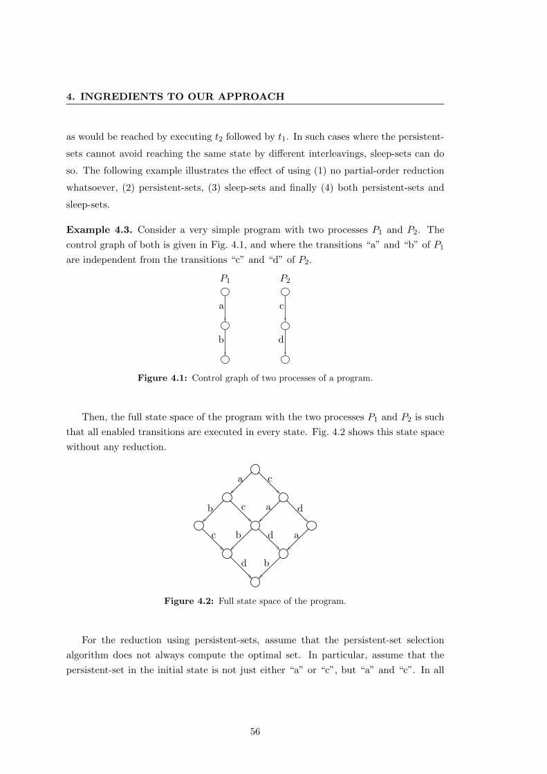
4. INGREDIENTS TO OUR APPROACH
as would be reached by executing t2 followed by t1. In such cases where the persistent-
sets cannot avoid reaching the same state by different interleavings, sleep-sets can do
so. The following example illustrates the effect of using (1) no partial-order reduction
whatsoever, (2) persistent-sets, (3) sleep-sets and finally (4) both persistent-sets and
sleep-sets.
Example 4.3. Consider a very simple program with two processes P1 and P2. The
control graph of both is given in Fig. 4.1, and where the transitions “a” and “b” of P1
are independent from the transitions “c” and “d” of P2.
P2
c
d
P1
b
a
Figure 4.1: Control graph of two processes of a program.
Then, the full state space of the program with the two processes P1 and P2 is such
that all enabled transitions are executed in every state. Fig. 4.2 shows this state space
without any reduction.
a
b a
b
c
dc
c a
d
b d
Figure 4.2: Full state space of the program.
For the reduction using persistent-sets, assume that the persistent-set selection
algorithm does not always compute the optimal set. In particular, assume that the
persistent-set in the initial state is not just either “a” or “c”, but “a” and “c”. In all
56
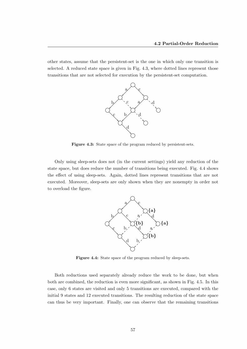
4.2 Partial-Order Reduction
other states, assume that the persistent-set is the one in which only one transition is
selected. A reduced state space is given in Fig. 4.3, where dotted lines represent those
transitions that are not selected for execution by the persistent-set computation.
a
b a
c
dc
c
d
b d
Figure 4.3: State space of the program reduced by persistent-sets.
Only using sleep-sets does not (in the current settings) yield any reduction of the
state space, but does reduce the number of transitions being executed. Fig. 4.4 shows
the effect of using sleep-sets. Again, dotted lines represent transitions that are not
executed. Moreover, sleep-sets are only shown when they are nonempty in order not
to overload the figure.
a
b a
b
c
dc
c a
d
b db
a
a
b
Figure 4.4: State space of the program reduced by sleep-sets.
Both reductions used separately already reduce the work to be done, but when
both are combined, the reduction is even more significant, as shown in Fig. 4.5. In this
case, only 6 states are visited and only 5 transitions are executed, compared with the
initial 9 states and 12 executed transitions. The resulting reduction of the state space
can thus be very important. Finally, one can observe that the remaining transitions
57
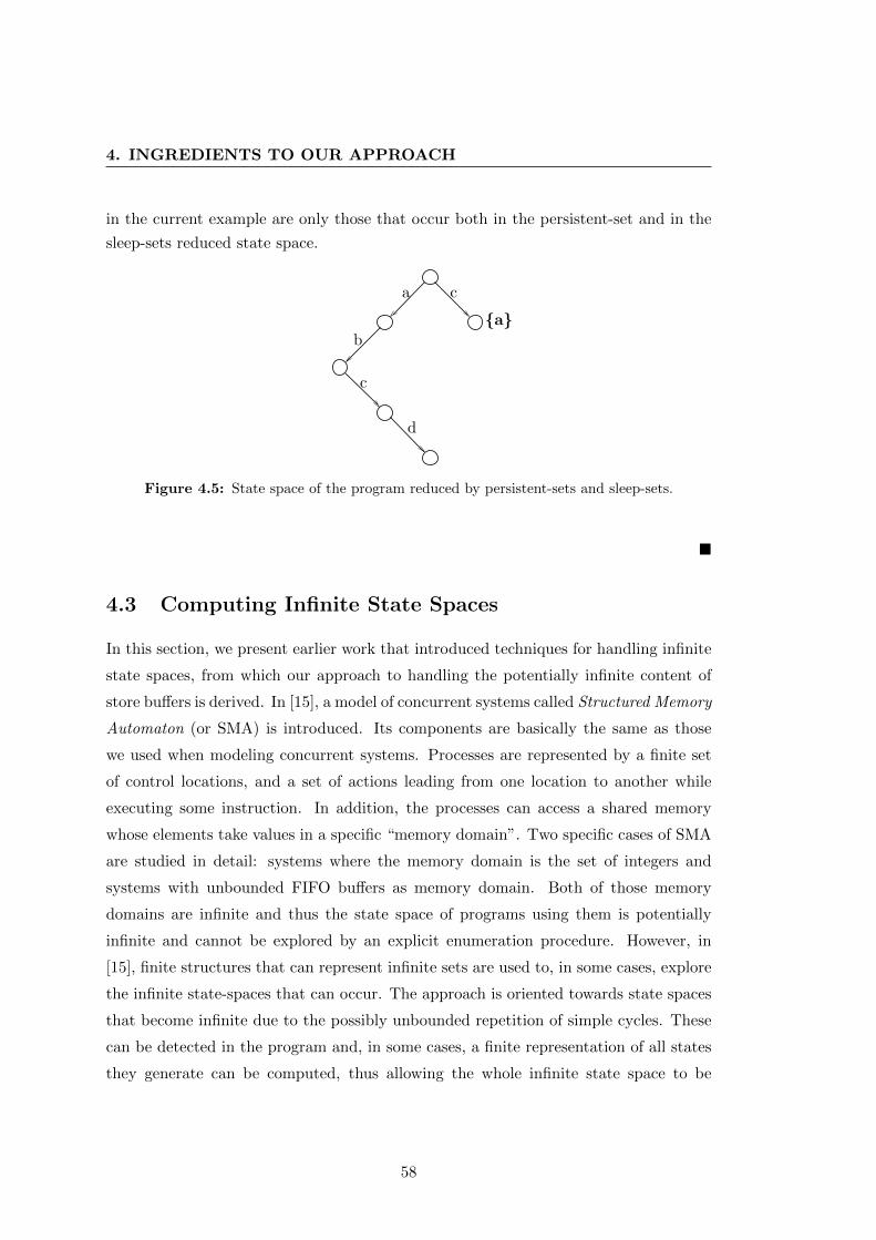
4. INGREDIENTS TO OUR APPROACH
in the current example are only those that occur both in the persistent-set and in the
sleep-sets reduced state space.
a
b
c
c
d
a
Figure 4.5: State space of the program reduced by persistent-sets and sleep-sets.
4.3 Computing Infinite State Spaces
In this section, we present earlier work that introduced techniques for handling infinite
state spaces, from which our approach to handling the potentially infinite content of
store buffers is derived. In [15], a model of concurrent systems called Structured Memory
Automaton (or SMA) is introduced. Its components are basically the same as those
we used when modeling concurrent systems. Processes are represented by a finite set
of control locations, and a set of actions leading from one location to another while
executing some instruction. In addition, the processes can access a shared memory
whose elements take values in a specific “memory domain”. Two specific cases of SMA
are studied in detail: systems where the memory domain is the set of integers and
systems with unbounded FIFO buffers as memory domain. Both of those memory
domains are infinite and thus the state space of programs using them is potentially
infinite and cannot be explored by an explicit enumeration procedure. However, in
[15], finite structures that can represent infinite sets are used to, in some cases, explore
the infinite state-spaces that can occur. The approach is oriented towards state spaces
that become infinite due to the possibly unbounded repetition of simple cycles. These
can be detected in the program and, in some cases, a finite representation of all states
they generate can be computed, thus allowing the whole infinite state space to be
58
4.4 Buffer Automata
explored in finite time. This is done by introducing meta-transitions that represent
the effect of iterating a loop an arbitrary number of times. Such meta-transitions can
be pre-computed, or being computed on-the-fly while exploring the state space. This
approach is fully developed in [15], but also appeared in earlier work, see [17, 18, 19, 72].
Technically, a meta-transition is computed by checking in a separate DFS if there is
a state reachable from the current state that only differs from it by the content of the
memory, and where this memory content has “grown” by the result of the operations
in the cycle. If this growth is repeated each time the cycle is executed, then one can
extrapolate the repeated growth by representing it symbolically, and hence a meta-
transition is created such that once this meta-transition is followed, the resulting state
represents all states reachable by executing the cycle one or several times.
In the general case, this approach is not guaranteed to terminate because not all
cycles can be accelerated, but it turns out that many programs having an infinite
state space have enough structure for their infinite state space to be captured in this
way. Also, [15] defines a set of sufficient conditions for a full exploration of the state
space to be possible. The intuition behind those conditions is that the program has a
control graph that can be flattened and for all cycles of which a meta-transition can be
computed. Additionally, it is required that there exists an order among these cycles,
leading to a sequential acceleration of all cycles.
We will adapt this approach to handling the buffering of processor writes appearing
in relaxed memory models. One peculiarity of the context of memory models is that
each processor has its own store buffer to which it has exclusive write access.
In the next section, we present the structure that will allow us to symbolically
represent sets of potentially unbounded buffer contents.
4.4 Buffer Automata
This section first gives an overview of the theoretical results that have been established
for TSO/PSO abstract machines. Then, we present a data structure, first introduced
in [45], that can symbolically represent not only one particular buffer content but also
sets of potentially infinite buffer contents.
As we saw in Sections 3.2 and 3.3, store buffers are used in the TSO or PSO
abstract machine models. The potential infinite nature of those store buffers makes
59
4. INGREDIENTS TO OUR APPROACH
it in general impossible to compute the full state space of programs analyzed under
these memory models. This was first shown in [11] and extended results appear in [12].
The proofs proceed by simulating TSO-machines (and PSO-machines) by lossy channel
systems (LCS) and vice-versa. Many theoretical results have been established for LCS
[5, 6, 25], and several implementations of state reachability exist [3, 4, 7]. Given the
existence of a simulation in both directions, all results established for LCS are also valid
for TSO/PSO-systems. Besides the undecidability of computing the entire state space
for LCS, it has been established that it is however possible to represent the full state
space (even if it cannot be computed), as well to decide reachability of a particular
state. This last result has been successfully exploited in [1, 2] in order to develop
an algorithm for deciding whether a state is reachable or not in the case of the TSO
memory model.
However, even if the full state space is not computable for every program, it can very
well be computed in many cases, using a finite representation of possibly infinite sets
of states. For those cases where a precise representation of the state space cannot be
computed, future work could combine the current approach with an over-abstraction
(or even under-abstraction) of the content of the store buffer in order to keep the
state space finite. For our purpose (using no abstraction), we define the concept of
buffer automata in Definition 4.4, taken from [45]. A buffer automaton is basically a
finite automaton, in which the alphabet is constituted by elements representing store
operations. The alphabet can be elements out ofM×D, whereM is the set of memory
locations and D is the data domain of the memory location. When more precision is
needed, the elements of the buffer are taken out of M×D × T , in order to allow the
identification of the executed and buffered store instruction in the program. A first
definition only considers the version using pairs of a memory location and a value (it
is only in Chapter 6 that a new definition of buffer automata becomes necessary in
Section 6.5.1).
Definition 4.4. A buffer automaton is a finite automaton A = (S,Σ,∆, S0, F ), where
S is a finite set of states,
Σ =M×D is the alphabet of buffer elements,
∆ ⊆ S × (Σ ∪ ε)× S is the transition relation,
S0 ⊆ S is a set of initial states, and
60
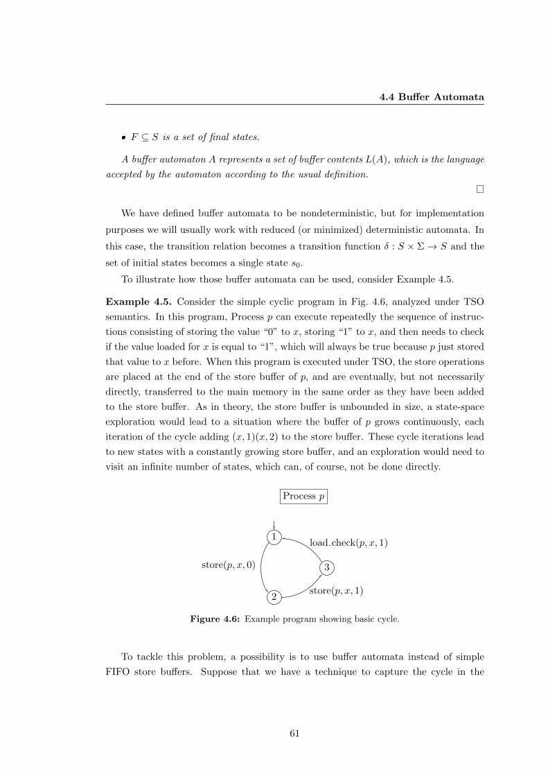
4.4 Buffer Automata
F ⊆ S is a set of final states.
A buffer automaton A represents a set of buffer contents L(A), which is the language
accepted by the automaton according to the usual definition.
We have defined buffer automata to be nondeterministic, but for implementation
purposes we will usually work with reduced (or minimized) deterministic automata. In
this case, the transition relation becomes a transition function δ : S × Σ → S and the
set of initial states becomes a single state s0.
To illustrate how those buffer automata can be used, consider Example 4.5.
Example 4.5. Consider the simple cyclic program in Fig. 4.6, analyzed under TSO
semantics. In this program, Process p can execute repeatedly the sequence of instruc-
tions consisting of storing the value “0” to x, storing “1” to x, and then needs to check
if the value loaded for x is equal to “1”, which will always be true because p just stored
that value to x before. When this program is executed under TSO, the store operations
are placed at the end of the store buffer of p, and are eventually, but not necessarily
directly, transferred to the main memory in the same order as they have been added
to the store buffer. As in theory, the store buffer is unbounded in size, a state-space
exploration would lead to a situation where the buffer of p grows continuously, each
iteration of the cycle adding (x, 1)(x, 2) to the store buffer. These cycle iterations lead
to new states with a constantly growing store buffer, and an exploration would need to
visit an infinite number of states, which can, of course, not be done directly.
1
2
store(p, x, 0)
load check(p, x, 1)
3
store(p, x, 1)
Process p
Figure 4.6: Example program showing basic cycle.
To tackle this problem, a possibility is to use buffer automata instead of simple
FIFO store buffers. Suppose that we have a technique to capture the cycle in the
61
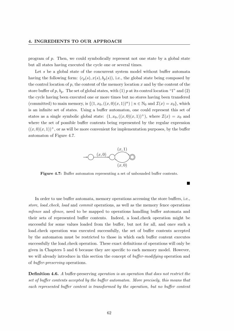
4. INGREDIENTS TO OUR APPROACH
program of p. Then, we could symbolically represent not one state by a global state
but all states having executed the cycle one or several times.
Let s be a global state of the concurrent system model without buffer automata
having the following form: (cp(s), x(s), bp(s)), i.e., the global state being composed by
the control location of p, the content of the memory location x and by the content of the
store buffer of p, bp. The set of global states, with (1) p at its control location “1” and (2)
the cycle having been executed one or more times but no stores having been transfered
(committed) to main memory, is (1, x0, ((x, 0)(x, 1))n) | n ∈ N0 and I(x) = x0, which
is an infinite set of states. Using a buffer automaton, one could represent this set of
states as a single symbolic global state: (1, x0, ((x, 0)(x, 1))+), where I(x) = x0 and
where the set of possible buffer contents being represented by the regular expression
((x, 0)(x, 1))+, or as will be more convenient for implementation purposes, by the buffer
automaton of Figure 4.7.
(x, 0)(x, 1)
(x, 0)
Figure 4.7: Buffer automaton representing a set of unbounded buffer contents.
In order to use buffer automata, memory operations accessing the store buffers, i.e.,
store, load check, load and commit operations, as well as the memory fence operations
mfence and sfence, need to be mapped to operations handling buffer automata and
their sets of represented buffer contents. Indeed, a load check operation might be
successful for some values loaded from the buffer, but not for all, and once such a
load check operation was executed successfully, the set of buffer contents accepted
by the automaton must be restricted to those in which each buffer content executes
successfully the load check operation. These exact definitions of operations will only be
given in Chapters 5 and 6 because they are specific to each memory model. However,
we will already introduce in this section the concept of buffer-modifying operation and
of buffer-preserving operations.
Definition 4.6. A buffer-preserving operation is an operation that does not restrict the
set of buffer contents accepted by the buffer automaton. More precisely, this means that
each represented buffer content is transformed by the operation, but no buffer content
62
4.4 Buffer Automata
for which the operation is impossible is eliminated. In other words, there is a one-
to-one relation between the set of buffer contents represented by the original buffer
automaton and the set of buffer contents represented by the buffer automaton obtained
after executing the operation.
Definition 4.7. A buffer-modifying operation is an operation that is not buffer-pre-
serving, i.e., an operation that restricts the set of accepted buffer contents of the buffer
automaton.
The example of a load check operation given above is such a buffer-modifying op-
eration which might restrict the accepted buffer contents. Conversely, the operations
store and lock, as well as local operations are examples of buffer-preserving operations.
Example 4.8. This example illustrates that store operations are buffer-preserving. Let
A be a buffer automaton accepting all the words that can be generated by the regular
expression (ab)∗, where a and b are random buffer elements. Let c be the symbol
representing (m, v). Executing the store operation store(p,m, v), where A represents
the buffer content of the buffer of p, the resulting buffer automaton A′ becomes (ab)∗ ·c(adding c to all contents). We then have a one-to-one relation between the contents in
A and the contents in A′.
Example 4.9. This example illustrates a buffer-modifying load-check operations. Let
A be the buffer automaton representing the buffer contents of the buffer associated to
process p, and accepting all the words that can be generated by the regular expression
(a)∗. Let a be (m, v), and let the value of m in the shared memory be v′. Then,
the operation load check(p,m, v) will restrict the resulting buffer automaton A′ to only
accept the buffer contents that can be generated by (a)+ to ensure that we will read
in any case the value v for m. Executing the operation load check(p,m, v′) would only
preserve the empty word in the resulting buffer. In both cases, we don’t have a one-to-
one relation between the contents in the corresponding buffer automata.
In the following, we will make use of a special buffer automaton accepting exclusively
the empty word. This buffer automaton is called empty buffer, and is introduced
formally in the following definition.
Definition 4.10. The empty buffer is a buffer automaton A such that L(A) = ε.
63

Chapter 5
Total Store Order
This chapter, together with Chapter 6, constitutes the heart of this thesis. Its aim
is to propose an approach for the verification of programs when the target processor
implements the Total Store Order (see Section 3.2) memory model, as do Intel’s x86
processors, but without restricting in any way the size of the store buffers. More specif-
ically, the techniques presented allow the verification of safety properties of programs
analyzed under TSO with unbounded memory buffers. Additionally, we propose an
approach that can modify a program in order to preserve a safety property, which is
satisfied by the program under SC, but violated when the program is moved onto a
TSO system. For the latter, the basic TSO memory model is not sufficient, and the
full x86-TSO model, which includes a memory fence operation, is clearly needed.
We start by giving the exact semantics of memory operations when buffer automata
(see Section 4.4) are used instead of simple FIFO store buffers. The reason for using
buffer automata resides in the fact that a buffer automaton may represent symbolically
sets of potentially unbounded buffer contents instead of representing only one particular
buffer content. Section 5.2 deals with the cycles that can be the origin of infinity in the
state space when allowing unbounded buffer contents. Some of them can be detected
and accelerated, others cannot. We give exact definitions, examples and intuitions for
the cycles that can be accelerated by our approach using buffer automata, as well as
examples and intuitions of cycles that cannot be accelerated. The buffer operations as
well as the concept of cycle acceleration have been introduced in [45]. In Section 4.2,
we did not give any information about how the partial-order reduction is going to be
applied in our setting. Thus, we need to give all the concrete definitions and implemen-
tation details for the partial-order reduction techniques we are using in the context of
TSO, see Section 5.3. The use of these in relaxed memory model verification was first
65
5. TOTAL STORE ORDER
introduced in [45], while [46] extended this use. Sections 5.4 and 5.5 respectively cover
the detection of deadlocks and the verification of safety properties. Last but not least,
Section 5.6 proposes a technique for modifying a program by iteratively inserting mem-
ory fences into it in order to preserve a safety-property (or the absence of deadlocks)
when that program is moved from an SC-machine to a TSO-machine. This result was
first published in [46].
5.1 Buffer Operations
In this section, we provide the precise semantics of all memory operations. For each
operation, we also specify whether it is buffer-preserving or buffer-modifying, which
is needed when dependence or independence of pairs of transitions is studied in Sec-
tion 5.3.1. In what follows, we use equivalently the terms store buffer and buffer.
Furthermore, when this does not lead to any ambiguity, we refer interchangeably to
a buffer and the buffer automaton representing its possible contents. Many examples
and illustrations are provided to help the reader understand the intuition behind the
operations that are described.
Recall that a global state s is composed of a control location for each process,
a buffer automaton associated to each process, a memory content for each memory
location and a value for the global lock, Lock, that can either be a process p ∈ P or
⊥. In the initial state, all buffers are set to the empty buffer (see Definition 4.10). The
control location for each process p ∈ P in a state s can be accessed by the function cp(s),
the memory content of variable m ∈M can be accessed by m(s), each buffer content of
p can be accessed by bp(s) (or Ap(s) when a set of buffer contents are represented by a
buffer automaton), and the value of the lock can be accessed by Lock(s). The current
global state will be denoted as s, and the successor state after executing t = `op→ `′
from s is denoted as s′, where op is the operation being executed. A second notation
for the computation of the successor state of s by executing t to reach s′ is to write
s′ = succ(s, t), where succ is the function returning the successor state of s reached by
executing t.
5.1.1 Store Operation
The first operation for which we need to give semantics is the store operation. It is the
following:
66
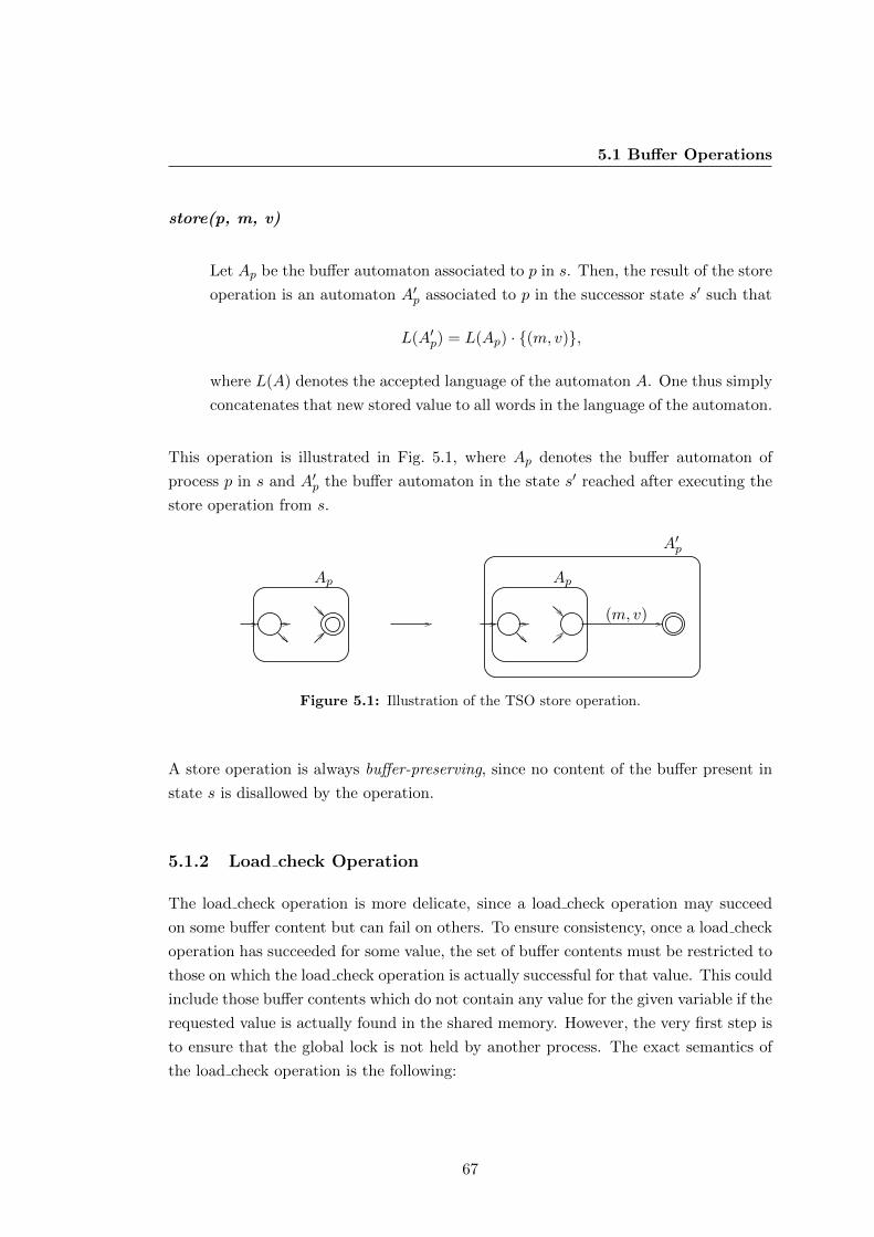
5.1 Buffer Operations
store(p, m, v)
Let Ap be the buffer automaton associated to p in s. Then, the result of the store
operation is an automaton A′p associated to p in the successor state s′ such that
L(A′p) = L(Ap) · (m, v),
where L(A) denotes the accepted language of the automaton A. One thus simply
concatenates that new stored value to all words in the language of the automaton.
This operation is illustrated in Fig. 5.1, where Ap denotes the buffer automaton of
process p in s and A′p the buffer automaton in the state s′ reached after executing the
store operation from s.
ApAp
(m, v)
A′p
Figure 5.1: Illustration of the TSO store operation.
A store operation is always buffer-preserving, since no content of the buffer present in
state s is disallowed by the operation.
5.1.2 Load check Operation
The load check operation is more delicate, since a load check operation may succeed
on some buffer content but can fail on others. To ensure consistency, once a load check
operation has succeeded for some value, the set of buffer contents must be restricted to
those on which the load check operation is actually successful for that value. This could
include those buffer contents which do not contain any value for the given variable if the
requested value is actually found in the shared memory. However, the very first step is
to ensure that the global lock is not held by another process. The exact semantics of
the load check operation is the following:
67
5. TOTAL STORE ORDER
load check(p, m, v)
If the global lock is held by another process, i.e., Lock(s) = p′, then the operation
cannot be executed.
Otherwise, we proceed as follows. For a load check operation to succeed, the
tested value must be found either in the store buffer or in main memory. Precisely,
a load check operation succeeds when at least one of the following two conditions
is satisfied:
1. The language
L1 = L(Ap) ∩ (Σ∗ · (m, v) · (Σ\(m,w) | w ∈ D)∗)
is nonempty, where Σ is the buffer alphabet and Ap is the buffer automaton
for p in s.
2. The language
L2 = L(Ap) ∩ (Σ\(m,w) | w ∈ D)∗
is nonempty and m(s) = v.
The first condition ensures that words are only retained in the set of accepted
buffer contents if, at one point in a retained word, there is a symbol representing
(m, v), followed only by symbols representing store operations accessing memory
locations other than m. The second condition ensures that, in the case where the
value of m in the shared memory (m(s)) is equal to v, only words that do not
contain any symbols representing store operations accessing memory location m
are retained.
The load check operation then leads to a state with a modified store buffer au-
tomaton A′p for p such that
L(A′p) = L1 ∪ L2
if m(s) = v and
L(A′p) = L1
otherwise. Of course, if L1 ∪ L2 = ∅, the load operation is simply not possible.
68
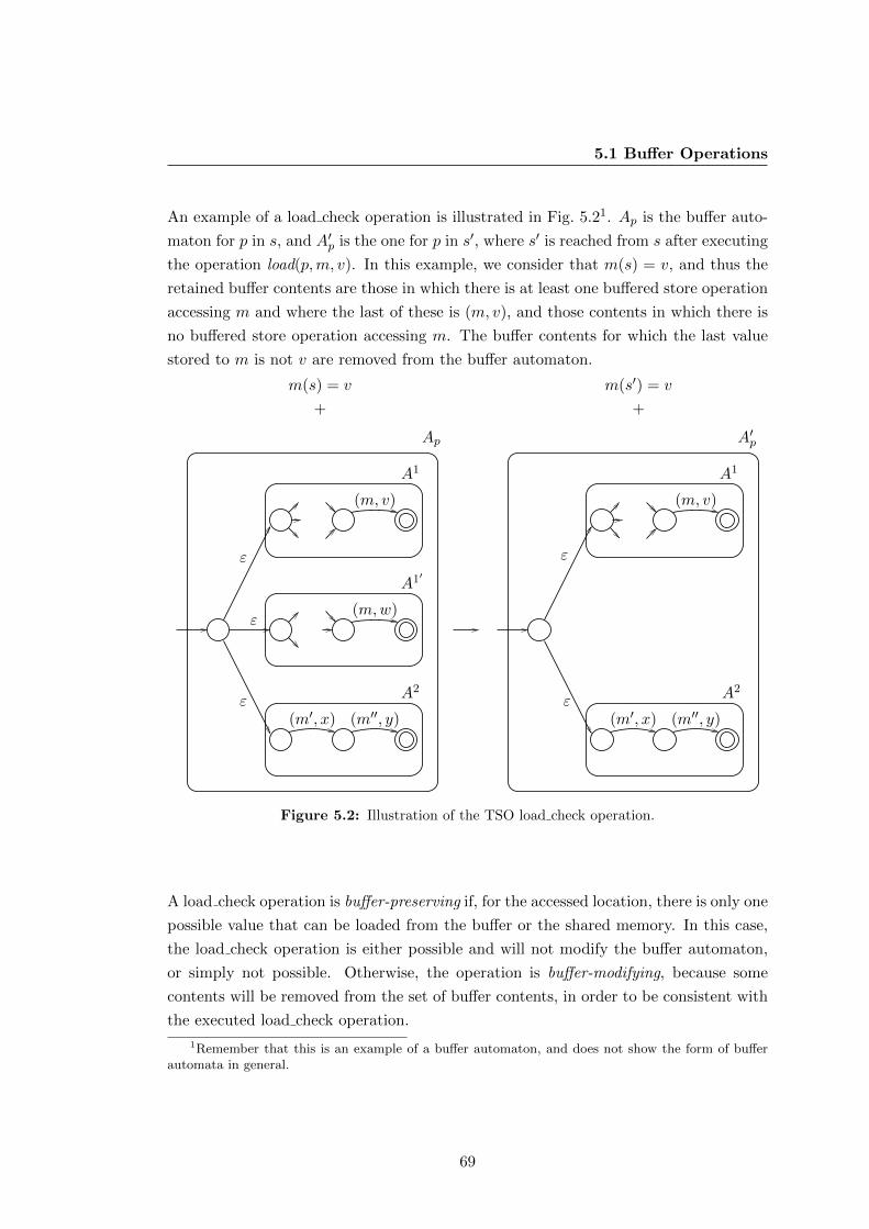
5.1 Buffer Operations
An example of a load check operation is illustrated in Fig. 5.21. Ap is the buffer auto-
maton for p in s, and A′p is the one for p in s′, where s′ is reached from s after executing
the operation load(p,m, v). In this example, we consider that m(s) = v, and thus the
retained buffer contents are those in which there is at least one buffered store operation
accessing m and where the last of these is (m, v), and those contents in which there is
no buffered store operation accessing m. The buffer contents for which the last value
stored to m is not v are removed from the buffer automaton.
ε(m′, x) (m′, x)
ε
(m, v)
(m′′, y)
(m,w)ε
ε
(m, v)
ε
(m′′, y)
A1
A1′
A2 A2
A1
A′pAp
m(s) = v
+
m(s′) = v
+
Figure 5.2: Illustration of the TSO load check operation.
A load check operation is buffer-preserving if, for the accessed location, there is only one
possible value that can be loaded from the buffer or the shared memory. In this case,
the load check operation is either possible and will not modify the buffer automaton,
or simply not possible. Otherwise, the operation is buffer-modifying, because some
contents will be removed from the set of buffer contents, in order to be consistent with
the executed load check operation.
1Remember that this is an example of a buffer automaton, and does not show the form of bufferautomata in general.
69
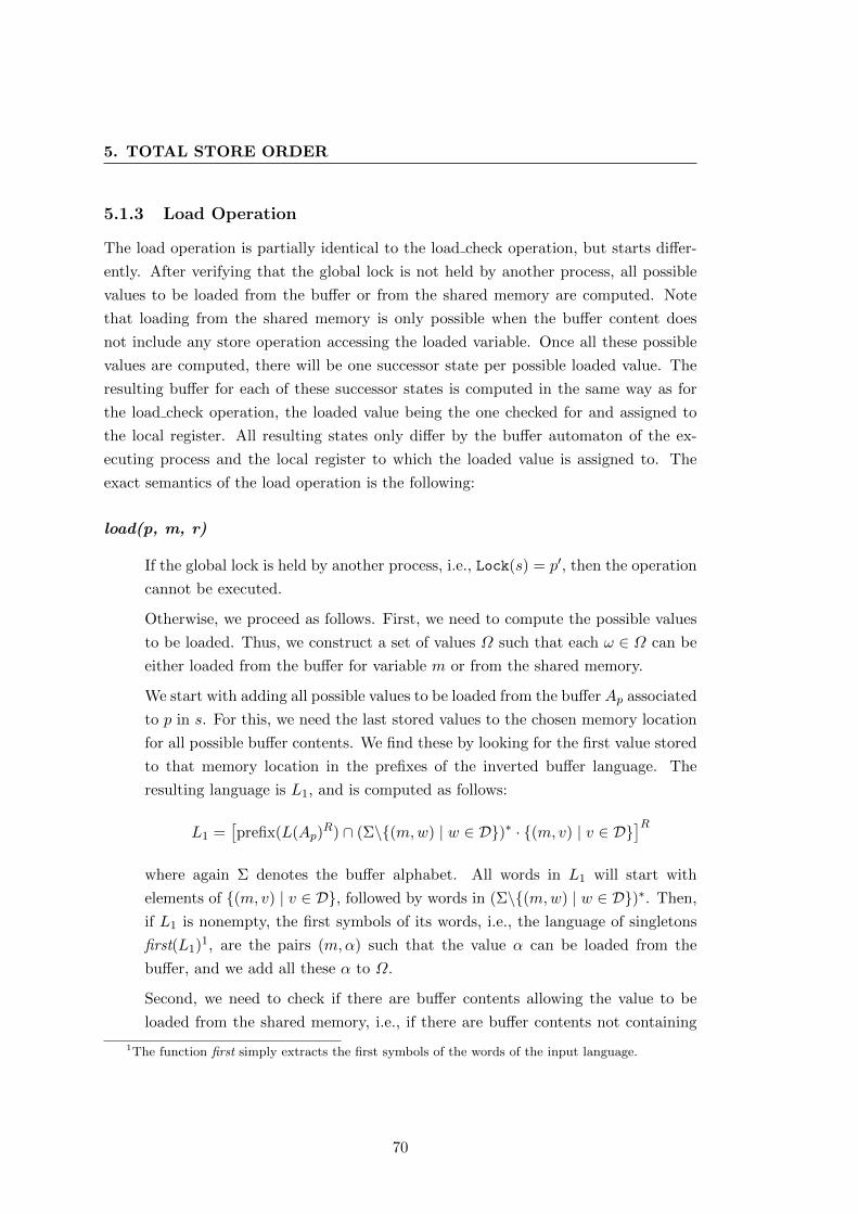
5. TOTAL STORE ORDER
5.1.3 Load Operation
The load operation is partially identical to the load check operation, but starts differ-
ently. After verifying that the global lock is not held by another process, all possible
values to be loaded from the buffer or from the shared memory are computed. Note
that loading from the shared memory is only possible when the buffer content does
not include any store operation accessing the loaded variable. Once all these possible
values are computed, there will be one successor state per possible loaded value. The
resulting buffer for each of these successor states is computed in the same way as for
the load check operation, the loaded value being the one checked for and assigned to
the local register. All resulting states only differ by the buffer automaton of the ex-
ecuting process and the local register to which the loaded value is assigned to. The
exact semantics of the load operation is the following:
load(p, m, r)
If the global lock is held by another process, i.e., Lock(s) = p′, then the operation
cannot be executed.
Otherwise, we proceed as follows. First, we need to compute the possible values
to be loaded. Thus, we construct a set of values Ω such that each ω ∈ Ω can be
either loaded from the buffer for variable m or from the shared memory.
We start with adding all possible values to be loaded from the buffer Ap associated
to p in s. For this, we need the last stored values to the chosen memory location
for all possible buffer contents. We find these by looking for the first value stored
to that memory location in the prefixes of the inverted buffer language. The
resulting language is L1, and is computed as follows:
L1 =[prefix(L(Ap)
R) ∩ (Σ\(m,w) | w ∈ D)∗ · (m, v) | v ∈ D]R
where again Σ denotes the buffer alphabet. All words in L1 will start with
elements of (m, v) | v ∈ D, followed by words in (Σ\(m,w) | w ∈ D)∗. Then,
if L1 is nonempty, the first symbols of its words, i.e., the language of singletons
first(L1)1, are the pairs (m,α) such that the value α can be loaded from the
buffer, and we add all these α to Ω.
Second, we need to check if there are buffer contents allowing the value to be
loaded from the shared memory, i.e., if there are buffer contents not containing
1The function first simply extracts the first symbols of the words of the input language.
70
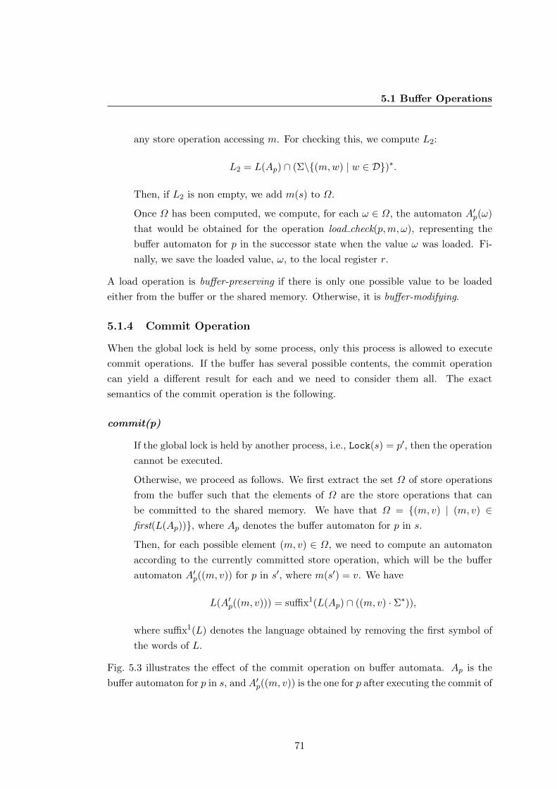
5.1 Buffer Operations
any store operation accessing m. For checking this, we compute L2:
L2 = L(Ap) ∩ (Σ\(m,w) | w ∈ D)∗.
Then, if L2 is non empty, we add m(s) to Ω.
Once Ω has been computed, we compute, for each ω ∈ Ω, the automaton A′p(ω)
that would be obtained for the operation load check(p,m, ω), representing the
buffer automaton for p in the successor state when the value ω was loaded. Fi-
nally, we save the loaded value, ω, to the local register r.
A load operation is buffer-preserving if there is only one possible value to be loaded
either from the buffer or the shared memory. Otherwise, it is buffer-modifying.
5.1.4 Commit Operation
When the global lock is held by some process, only this process is allowed to execute
commit operations. If the buffer has several possible contents, the commit operation
can yield a different result for each and we need to consider them all. The exact
semantics of the commit operation is the following.
commit(p)
If the global lock is held by another process, i.e., Lock(s) = p′, then the operation
cannot be executed.
Otherwise, we proceed as follows. We first extract the set Ω of store operations
from the buffer such that the elements of Ω are the store operations that can
be committed to the shared memory. We have that Ω = (m, v) | (m, v) ∈first(L(Ap)), where Ap denotes the buffer automaton for p in s.
Then, for each possible element (m, v) ∈ Ω, we need to compute an automaton
according to the currently committed store operation, which will be the buffer
automaton A′p((m, v)) for p in s′, where m(s′) = v. We have
L(A′p((m, v))) = suffix1(L(Ap) ∩ ((m, v) · Σ∗)),
where suffix1(L) denotes the language obtained by removing the first symbol of
the words of L.
Fig. 5.3 illustrates the effect of the commit operation on buffer automata. Ap is the
buffer automaton for p in s, and A′p((m, v)) is the one for p after executing the commit of
71
5. TOTAL STORE ORDER
(m, v). In this example, there are two possible store operations that can be committed.
We consider each of them, while restricting the resulting automaton in such a way that
the accepted language contains only the words that originally (before executing the
commit) started with the selected committed store operation.
(x,1)
(x,0)
x(s′)← 1 +
x(s′′)← 0 +
A′p((x, 1))
A′p((x, 0))
Ap
A1
A2
Figure 5.3: Illustration of the TSO commit operation.
The condition for a commit operation to be buffer-preserving is the following. If the
function first(Ap) only returns one possible pair (m, v) and if the buffer automaton does
not accept the empty word, then the commit operation is buffer-preserving, because
all contents start with the same pair, and no restriction is going to be made on the
contents. Otherwise, the commit is buffer-modifying.
5.1.5 Mfence Operation
The mfence operation is a simpler operation. The mfence operation is only possible
if the buffer automaton of the executing process accepts, possibly among others, the
empty word. However, once the mfence operation is executed, the buffer is required
to only have the empty word as possible content, meaning that the mfence only is
possible on that sub-state having the empty word as buffer content. The semantics of
the mfence operation is the following.
mfence(p)
First, one needs to check if the accepted language L(Ap) of the buffer automaton
Ap for p in s contains the empty buffer, i.e., if ε ∈ L(Ap). If this is the case, the
72
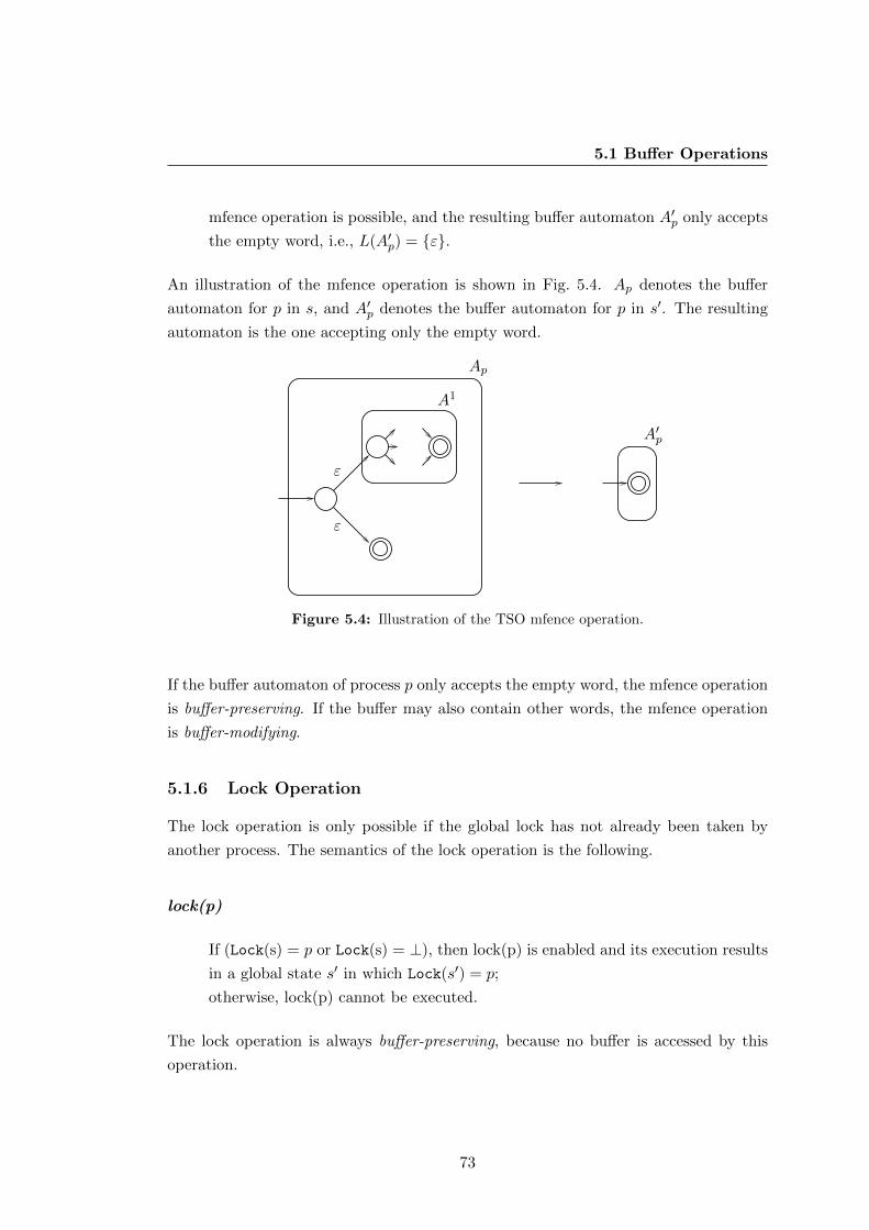
5.1 Buffer Operations
mfence operation is possible, and the resulting buffer automaton A′p only accepts
the empty word, i.e., L(A′p) = ε.
An illustration of the mfence operation is shown in Fig. 5.4. Ap denotes the buffer
automaton for p in s, and A′p denotes the buffer automaton for p in s′. The resulting
automaton is the one accepting only the empty word.
ε
ε
Ap
A1
A′p
Figure 5.4: Illustration of the TSO mfence operation.
If the buffer automaton of process p only accepts the empty word, the mfence operation
is buffer-preserving. If the buffer may also contain other words, the mfence operation
is buffer-modifying.
5.1.6 Lock Operation
The lock operation is only possible if the global lock has not already been taken by
another process. The semantics of the lock operation is the following.
lock(p)
If (Lock(s) = p or Lock(s) = ⊥), then lock(p) is enabled and its execution results
in a global state s′ in which Lock(s′) = p;
otherwise, lock(p) cannot be executed.
The lock operation is always buffer-preserving, because no buffer is accessed by this
operation.
73
5. TOTAL STORE ORDER
5.1.7 Unlock Operation
The unlock operation can only be completed if the sequence of locked instructions
(and consequently also all previous operations) is entirely visible globally. The unlock
operation is thus only possible when the buffer of the executing process has the empty
word as possible content. If so, the result of the unlock operation is to release the lock
and the buffer is set to be empty. If not, the unlock operation is not possible and the
Lock is still held by the executing process. The semantics is the following.
unlock(p)
If (Lock(s) = p and ε ∈ L(Ap(s))), then unlock operation can be executed and
its execution results in a state s′ where Lock(s′) =⊥ and L(Ap(s′)) = ε;
otherwise, unlock(p) cannot be executed.
The unlock operation is buffer-preserving if the buffer of the executing process only
contains the empty word. If the buffer contains other contents alongside the empty
word, the operation is buffer-modifying because the buffer automaton will be set to just
contain the empty word.
5.1.8 Local Operation
In terms of global state reachability, one does not need any local variable and purely
local operations, everything could be modeled without such variables. However, to
allow an effective input language and exploration of the state space, we need local
variables as well as purely local operations working on those local variables. Thus, our
system does propose many local operations, like assignments, Boolean conditions and
local variable arithmetic. However, when questioning independence of operations, one
can merge them together into the type “local operation”.
Any local operation is always buffer-preserving.
5.1.9 Discussion on Operations
There are some operations, such as mfence and unlock, that may not be executable
because there is some condition on the buffer automaton which is not fulfilled. If such
an operation is not possible in some global state s, it will eventually become so in some
successor state of s because of the nondeterministic execution of commit operations in
every global state.
74
5.2 Cycles
In order to formalize this nondeterministic transfer of the elements of the buffers
to the shared memory, we add a new component to our system: the buffer-emptying
process, written pb, whose only task is to execute commit operations on any buffer.
This process only has one control location, and its enabled transitions in a state s are
the possible commit operations to be executed on any buffer, while pb always stays in
its single state. Every commit(p) operation becomes thus an operation where process
pb is the active one. This modeling will make it easier to determine dependence or
independence of transitions when considering partial-order reduction (Section 5.3).
In Section 5.2, we will introduce the technique for accelerating cycles. This also
amounts to an operation on buffer automata, but one that models the repeated execu-
tion of a program cycle.
In Section 5.3, we will turn to the definition of independence among transitions,
which will also be conditioned on the contents of the buffers.
5.2 Cycles
This section proposes a way for tackling the problem of the potentially infinite store
buffers used in our TSO-machine model. In Section 4.4, we already introduced a
data structure, buffer automata, that allows representing sets of unbounded buffer
contents within a finite automaton. We also mapped the memory access operations onto
operations on this structure, but we have not yet introduced a method for computing
buffer automata representing sets of buffer contents while exploring the state space of
a program. This section introduces such a method that is based on the computation
of buffer automata representing all buffer contents that can be obtained by repeatedly
executing a cycle. We consider only cycles resulting in a state in which a single process
has a modified buffer. It might seem too restrictive to only consider this type of cycle,
but given the fact that the store buffers are exclusively associated to a single process,
there is only one process can make a given buffer grow. Though we only focus on these
simple cycles, we need to mention that other types of cycles do exist and can make the
buffers grow in a way that our approach cannot detect. However, such situations are
rare in practice, and our approach can handle a large set of programs and provides very
competitive results with respect to other approaches. As a first step, we will characterize
the type of cycles we can accelerate and present the theory underlying the acceleration
of these cycles. Then, we will present our implementation of cycle acceleration, and
prove it to be consistent with the theoretical approach provided beforehand.
75
5. TOTAL STORE ORDER
5.2.1 Cycle Acceleration in Theory
As we only consider systems that are finite-state under SC, the store buffers are the
only part in a TSO system which can potentially turn those finite-state systems into
infinite-state systems. The construction of the state space of an infinite-state system is
in general not possible, because the explicit and exhaustive enumeration of the infinite
number of states cannot be done. However, if the nature of the infinity is only due to
the unbounded growth of the store buffers due to the repeated execution of a cycle of
a particular type, one can compute in a single step the effect of the repeated execution
of this cycle, and hence make the construction of the state space possible.
The intuition behind the type of cycles we can accelerate and the acceleration
technique is quite simple. If the only effect of executing a cyclic sequence of operations
of all processes (those in P and the buffer emptying process pb) is that the contents of
the buffer of p in L(Ap) have been extended by some suffix while all other parts of the
system are identical before and after executing the cyclic sequence, it is easy to modify
Ap such that L(Ap) contains all buffer contents that can be obtained after repeatedly
executing this sequence.
In order to establish formally the acceleration technique, we first need to define the
concept of two sets of buffer contents being load-equivalent, meaning that both allow
loading exactly the same value(s) for each global variable. This concept is given in
Definition 5.1, and is used to ensure that, even if the buffer of the process has grown
during the execution of a given sequence of operations, the process has exactly the same
view of the values that can be loaded from the buffer before and after having executed
the sequence.
Definition 5.1. Two buffer automata A1 and A2 are load-equivalent, denoted A1 ≡ld
A2, if both A1 and A2 allow loading exactly the same set of values for all m ∈M.
The procedure for computing the set of values that can be loaded from a buffer
automaton has been given in Section 5.1.3 defining the load operation on a buffer
automaton. In the current setting, we do however not allow loading the value from the
shared memory, because we want the buffer automata to be load-equivalent without
taking into account the values of the shared memory. The procedure to compute the
set values that can be loaded is thus adapted accordingly.
The next condition we need to ensure in order to successfully detect a cycle that
can be accelerated (those that only make the buffer of p grow) is that the set of buffer
contents in Ap must not be restricted between the start and the end of the cycle, either
76
5.2 Cycles
by a commit to remove an element of the buffer or by any other operation of p that is
buffer-modifying. This can easily be verified by checking that there are no operations
of the following types between the starting and ending points of the cycle: commit(p)
and any buffer-modifying operation of p. In addition, there is no reason to allow for
example an mfence(p) operation during a cycle. Indeed, such an mfence during a cyclic
sequence would require the buffer to be emptied at least once during the cycle, ensuring
that the buffer cannot grow to become unbounded, and thus such a cycle cannot be
the origin of an infinite number of states. Similarly, one can argue for not allowing any
lock(p)/unlock(p) operation during the cycle. All those conditions are brought together
in Definition 5.2.
Definition 5.2. A sequence of operations from state s1 to state s2 is p-buffer-growing
if none of the following operations, executed by p (on p’s buffer for the commit), are
encountered between s1 and s2:
commit,
mfence,
lock,
unlock,
buffer-modifying load/load check.
Before providing the conditions under which cycles can be accelerated, we introduce
some additional notation. When we want express that states s1 and s2 are equivalent
except for the contents in L(Ap), we write s1 ≡\Ap s2. Formally, we have Definition 5.3.
Recall that cp(s),m(s), and Ap(s) access the control location of p in s, the memory
content of m in s and the buffer automaton associated to p in s.
Definition 5.3. Two states s1 and s2 are equivalent except for the buffer contents of
process p, written as s1 ≡\Ap s2, if:
∀p ∈ P : cp(s1) = cp(s2)
∀m ∈M : m(s1) = m(s2)
∀p′ ∈ P \ p : L(Ap′(s1)) = L(Ap′(s2))
77
5. TOTAL STORE ORDER
Now, we can define the conditions under which the sequence leading from a state
s1 to s2 only grows the buffer content of one process and can be repeated.
Definition 5.4. A sequence s1 → s2 from a state s1 to a state s2 satisfies the cycle-
condition for a process p if
s1 ≡\Ap s2,
Ap(s2) ≡ld Ap(s1),
s1 → s2 is p-buffer-growing.
For a sequence satisfying the cycle-condition, one can compute a buffer automaton
representing all buffer contents of p that are generated during the execution of the se-
quence s1 → s2, written Ap(s1 → s2) and such that L(Ap(s2)) = L(Ap(s1)) ·L(Ap(s1 →s2)), see Lemma 5.5. The automaton L(Ap(s1 → s2)) can represent a single buffer con-
tent or even a set of buffer contents if cycles are detected and accelerated between s1
and s2.
Lemma 5.5. Let seq be a cyclic sequence from s1 to s2 satisfying the cycle-condition
for process p. Then, all buffer contents that are generated between s1 and s2 for p are
in L(Ap(s1 → s2)) such that L(Ap(s2)) = L(Ap(s1)) · L(Ap(s1 → s2)), meaning that
the resulting buffer for p in s2 is the concatenation of the contents of Ap(s1) and the
contents generated between s1 and s2.
Proof. This is immediate because of the conditions in the cycle-condition of Defini-
tion 5.4 that are satisfied. Indeed, as these conditions imply that the sequence seq is
p-buffer-growing, the contents of the buffer of p have not been restricted in any ways
during seq. The only operations that may effect Ap during seq are store operations
and/or the acceleration of an (or several) inner cycle(s) detected between s1 and s2.
Thus, we know that L(Ap(s2)) = L(Ap(s1)) · L1, because the L(Ap(s1))-part is left
unchanged during seq, and L1 represents all contents that are generated during seq for
p, which is labeled L(Ap(s1 → s2)).
Accelerating such a detected cycle consists of modifying the buffer automaton such
that it represents all buffer contents obtained after repeatedly executing the cycle.
Moreover, we will also consider the, in practice rather rare, situation where several
cycles between the same pair of states need to be conjointly accelerated. For this, we
78
5.2 Cycles
introduce some further definitions, which will then lead to theorems of accelerating
cycles.
Definition 5.6. A sequence of operations is cyclic-strong for process p if it satisfies
the cycle condition of Definition 5.4 for process p and contains at least one operation
executed by the process p.
Definition 5.7. Given a state s, the sequences in the set SEQ = seq1, . . . , seqkoriginating from s are mixable for p if:
∃` ∀seq ∈ SEQ : seq is cyclic-strong for p and leads process p from ` to `,
where ` is a control location of process p.
Definition 5.7 ensures that, for process p, the view of the memory is identical after
executing any (or none) of the mixable sequences, implying that there is no difference
on the possible future behaviors of p whether none or one of the mixable sequences
is executed. Moreover, as the cycle conditions are also fulfilled, all other processes
p′ ∈ P \ p do not see any difference in the state right before and in the state right
after executing the cycle, which implies that they have exactly the same possible fu-
ture behaviors in these states. The following theorem establishes that executing any
sequence of a set of mixable sequences does not modify the possible future behaviors
of any of the processes of P.
Theorem 5.8. Consider a state s and a set SEQ of mixable sequences for p originating
from s. Executing a sequence in SEQ entirely does not modify the possible future
behaviors of the program.
Proof. For any process p′ ∈ P \ p, it is obvious that there is no difference in the
possible future behaviors of these processes. Indeed, as the conditions on a set of
mixable sequences for p imply that the conditions of Definition 5.7 for process p are
satisfied, we have the following conditions fulfilled, where si denotes the state after the
execution of the mixable sequence seqi ∈ SEQ for p:
∀p′ ∈ P \ p : cp′(s) = cp′(si)
∀m ∈M : m(s) = m(si)
∀p′ ∈ P \ p : Ap′(s) = Ap′(si)
79
5. TOTAL STORE ORDER
seqi is p-buffer-growing.
This directly implies that all processes p′ 6= p do not see any difference in the state
reached before and after executing seqi ∈ SEQ.
For the process p, the statement also holds. Indeed, the conditions of the theorem
ensure that the view of the memory is identical before and after the execution of any of
the mixable sequences in SEQ, ensuring that the same possible future behaviors exist
for p before and after the execution of one of the mixable sequences.
We conclude that, starting from s, executing entirely a sequence in SEQ does not
modify the possible future behaviors for all processes of P.
After establishing this theorem, we can prove that the sequences of a set of mixable
sequences SEQ of a process p can be executed repeatedly and mixed, while the only
effect of executing one of the mixable sequences seqi ∈ SEQ is to add at the end of
the buffer contents of p the buffer contents generated while executing seqi for p. We
first establish, as a consequence of Theorem 5.8, that the single execution of one se-
quence seqi of a set of mixable sequences SEQ for p originating from s only has the
effect of adding at the end of the buffer contents of p the buffer contents that are gen-
erated while executing seqi. Afterwards, Theorem 5.10 establishes that these mixable
sequences can be repeated and mixed any number of times, while each execution of
such a sequence only adds the corresponding buffer contents at the end of each buffer
content of p. Finally, Theorem 5.11 establishes that the repeated and mixed execution
of mixable sequences of process p can be computed in a single step by modifying the
buffer content of p such that it represents the repeated and mixed execution of these
mixable sequences, given by Equation 5.1.
Lemma 5.9. Consider a state s for which there exists a set of mixable sequences SEQ
for the process p. Then, the execution of any sequence seqi ∈ SEQ only has the effect
of adding at the end of the buffer contents of p the buffer contents that are generated
for p while executing seqi.
Proof. This is a direct consequence of Theorem 5.8. Indeed, as the execution of a
sequence of the set of mixable sequences SEQ does not modify the possible future
behaviors of the processes in P, the only effect of the execution of seqi ∈ SEQ is to add
at the end of the buffer contents of p the buffer contents in L(Aseqi) that are generated
while executing seqi.
80
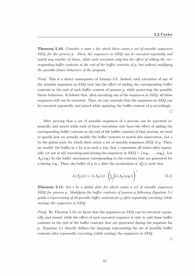
5.2 Cycles
Theorem 5.10. Consider a state s for which there exists a set of mixable sequences
SEQ for the process p. Then, the sequences in SEQ can be executed repeatedly and
mixed any number of times, while each execution only has the effect of adding the cor-
responding buffer contents at the end of the buffer contents of p, but without modifying
the possible future behaviors of the program.
Proof. This is a direct consequence of Lemma 5.9. Indeed, each execution of any of
the mixable sequences in SEQ only has the effect of adding the corresponding buffer
contents at the end of each buffer content of process p, while preserving the possible
future behaviors. It follows that, after executing one of the sequences in SEQ, all these
sequences still can be executed. Thus, we can conclude that the sequences in SEQ can
be executed repeatedly and mixed while updating the buffer content of p accordingly.
After proving that a set of mixable sequences of a process can be executed re-
peatedly and mixed while each of these executions only have the effect of adding the
corresponding buffer contents at the end of the buffer contents of that process, we need
to specify how we actually modify the buffer contents to match this observation. Let s
be the global state for which there exists a set of mixable sequences SEQ of p. Then,
we modify the buffer in s for p in such a way that s represents all states after repeat-
edly (or not at all) executing and mixing the sequences in SEQ = seq1, . . . , seqk. Let
Ap(seqi) be the buffer automaton corresponding to the contents that are generated for
p during seqi. Then, the buffer of p in s after the acceleration is A′p(s) such that
L(A′p(s)) = L(Ap(s)) ·
(⋃i
L(Ap(seqi))
)∗(5.1)
Theorem 5.11. Let s be a global state for which exists a set of mixable sequences
SEQ for process p. Modifying the buffer contents of process p following Equation 5.1
yields a representing of all possible buffer contents for p after repeatedly executing (while
mixing) the sequences in SEQ.
Proof. By Theorem 5.10, we know that the sequences in SEQ can be executed repeat-
edly and mixed, while the effect of each executed sequence is only to add those buffer
contents at the end of the buffer contents that are generated during the sequence for
p. Equation 5.1 directly defines the language representing the set of possible buffer
contents after repeatedly executing (while mixing) the sequences in SEQ.
81
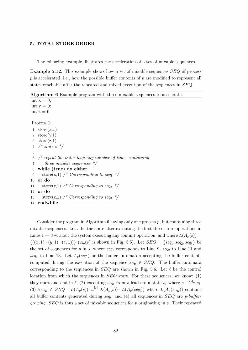
5. TOTAL STORE ORDER
The following example illustrates the acceleration of a set of mixable sequences.
Example 5.12. This example shows how a set of mixable sequences SEQ of process
p is accelerated, i.e., how the possible buffer contents of p are modified to represent all
states reachable after the repeated and mixed execution of the sequences in SEQ.
Algorithm 6 Example program with three mixable sequences to accelerate.
int x = 0;int y = 0;int z = 0;
Process 1:
1: store(x,1)2: store(y,1)3: store(z,1)4: /* state s */5:
6: /* repeat the outer loop any number of time, containing7: three mixable sequences */8: while (true) do either9: store(x,1) /* Corresponding to seq1 */
10: or do11: store(y,1) /* Corresponding to seq2 */12: or do13: store(z,1) /* Corresponding to seq3 */14: endwhile
Consider the program in Algorithm 6 having only one process p, but containing three
mixable sequences. Let s be the state after executing the first three store operations in
Lines 1 — 3 without the system executing any commit operation, and where L(Ap(s)) =
((x, 1) · (y, 1) · (z, 1)) (Ap(s) is shown in Fig. 5.5). Let SEQ = seq1, seq2, seq3 be
the set of sequences for p in s, where seq1 corresponds to Line 9, seq2 to Line 11 and
seq3 to Line 13. Let Ap(seqi) be the buffer automaton accepting the buffer contents
computed during the execution of the sequence seqi ∈ SEQ. The buffer automata
corresponding to the sequences in SEQ are shown in Fig. 5.6. Let ` be the control
location from which the sequences in SEQ start. For these sequences, we know: (1)
they start and end in `, (2) executing seqi from s leads to a state si where s ≡\Ap si,
(3) ∀seqi ∈ SEQ : L(Ap(s)) ≡ld L(Ap(s)) · L(Ap(seqi)) where L(Ap(seqi)) contains
all buffer contents generated during seqi, and (4) all sequences in SEQ are p-buffer-
growing. SEQ is thus a set of mixable sequences for p originating in s. Their repeated
82
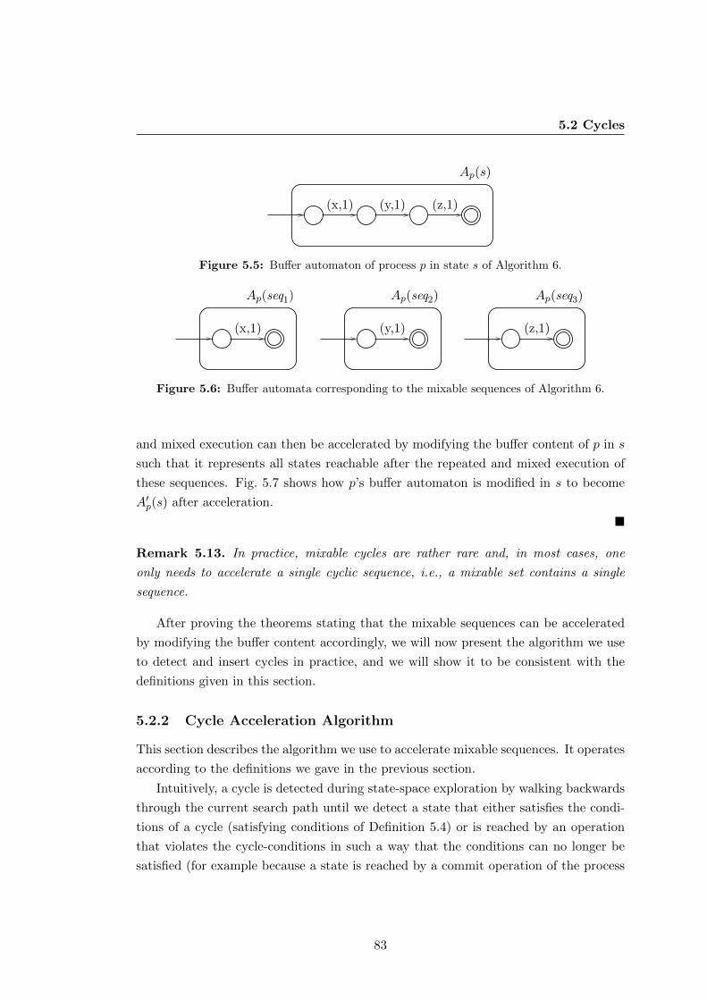
5.2 Cycles
(x,1)
Ap(s)
(y,1) (z,1)
Figure 5.5: Buffer automaton of process p in state s of Algorithm 6.
(x,1)
Ap(seq1)
(y,1)
Ap(seq2)
(z,1)
Ap(seq3)
Figure 5.6: Buffer automata corresponding to the mixable sequences of Algorithm 6.
and mixed execution can then be accelerated by modifying the buffer content of p in s
such that it represents all states reachable after the repeated and mixed execution of
these sequences. Fig. 5.7 shows how p’s buffer automaton is modified in s to become
A′p(s) after acceleration.
Remark 5.13. In practice, mixable cycles are rather rare and, in most cases, one
only needs to accelerate a single cyclic sequence, i.e., a mixable set contains a single
sequence.
After proving the theorems stating that the mixable sequences can be accelerated
by modifying the buffer content accordingly, we will now present the algorithm we use
to detect and insert cycles in practice, and we will show it to be consistent with the
definitions given in this section.
5.2.2 Cycle Acceleration Algorithm
This section describes the algorithm we use to accelerate mixable sequences. It operates
according to the definitions we gave in the previous section.
Intuitively, a cycle is detected during state-space exploration by walking backwards
through the current search path until we detect a state that either satisfies the condi-
tions of a cycle (satisfying conditions of Definition 5.4) or is reached by an operation
that violates the cycle-conditions in such a way that the conditions can no longer be
satisfied (for example because a state is reached by a commit operation of the process
83
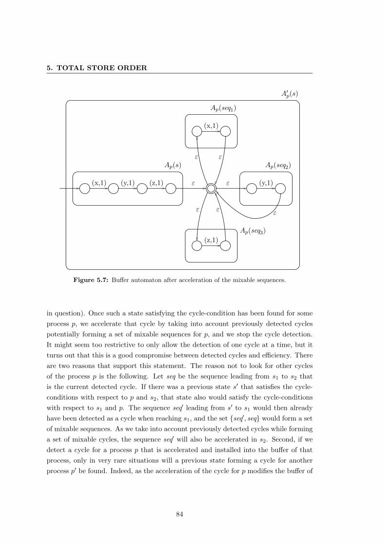
5. TOTAL STORE ORDER
(x,1) (y,1) (z,1)
Ap(s)
ε
(z,1)
Ap(seq3)
ε ε
ε (y,1)
Ap(seq2)
ε
(x,1)
Ap(seq1)
ε ε
A′p(s)
Figure 5.7: Buffer automaton after acceleration of the mixable sequences.
in question). Once such a state satisfying the cycle-condition has been found for some
process p, we accelerate that cycle by taking into account previously detected cycles
potentially forming a set of mixable sequences for p, and we stop the cycle detection.
It might seem too restrictive to only allow the detection of one cycle at a time, but it
turns out that this is a good compromise between detected cycles and efficiency. There
are two reasons that support this statement. The reason not to look for other cycles
of the process p is the following. Let seq be the sequence leading from s1 to s2 that
is the current detected cycle. If there was a previous state s′ that satisfies the cycle-
conditions with respect to p and s2, that state also would satisfy the cycle-conditions
with respect to s1 and p. The sequence seq′ leading from s′ to s1 would then already
have been detected as a cycle when reaching s1, and the set seq′, seq would form a set
of mixable sequences. As we take into account previously detected cycles while forming
a set of mixable cycles, the sequence seq′ will also be accelerated in s2. Second, if we
detect a cycle for a process p that is accelerated and installed into the buffer of that
process, only in very rare situations will a previous state forming a cycle for another
process p′ be found. Indeed, as the acceleration of the cycle for p modifies the buffer of
84
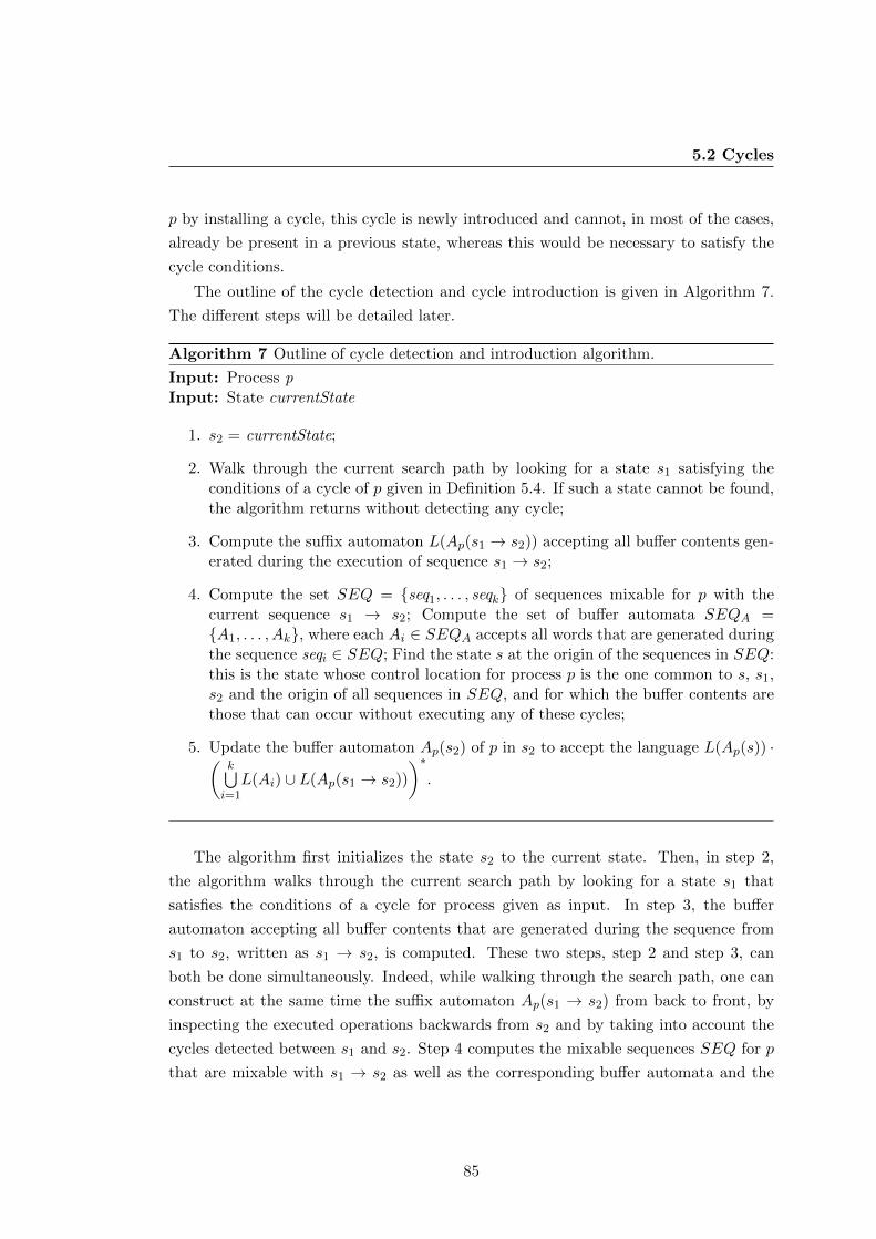
5.2 Cycles
p by installing a cycle, this cycle is newly introduced and cannot, in most of the cases,
already be present in a previous state, whereas this would be necessary to satisfy the
cycle conditions.
The outline of the cycle detection and cycle introduction is given in Algorithm 7.
The different steps will be detailed later.
Algorithm 7 Outline of cycle detection and introduction algorithm.
Input: Process pInput: State currentState
1. s2 = currentState;
2. Walk through the current search path by looking for a state s1 satisfying theconditions of a cycle of p given in Definition 5.4. If such a state cannot be found,the algorithm returns without detecting any cycle;
3. Compute the suffix automaton L(Ap(s1 → s2)) accepting all buffer contents gen-erated during the execution of sequence s1 → s2;
4. Compute the set SEQ = seq1, . . . , seqk of sequences mixable for p with thecurrent sequence s1 → s2; Compute the set of buffer automata SEQA =A1, . . . , Ak, where each Ai ∈ SEQA accepts all words that are generated duringthe sequence seqi ∈ SEQ; Find the state s at the origin of the sequences in SEQ:this is the state whose control location for process p is the one common to s, s1,s2 and the origin of all sequences in SEQ, and for which the buffer contents arethose that can occur without executing any of these cycles;
5. Update the buffer automaton Ap(s2) of p in s2 to accept the language L(Ap(s)) ·(k⋃
i=1L(Ai) ∪ L(Ap(s1 → s2))
)∗.
The algorithm first initializes the state s2 to the current state. Then, in step 2,
the algorithm walks through the current search path by looking for a state s1 that
satisfies the conditions of a cycle for process given as input. In step 3, the buffer
automaton accepting all buffer contents that are generated during the sequence from
s1 to s2, written as s1 → s2, is computed. These two steps, step 2 and step 3, can
both be done simultaneously. Indeed, while walking through the search path, one can
construct at the same time the suffix automaton Ap(s1 → s2) from back to front, by
inspecting the executed operations backwards from s2 and by taking into account the
cycles detected between s1 and s2. Step 4 computes the mixable sequences SEQ for p
that are mixable with s1 → s2 as well as the corresponding buffer automata and the
85
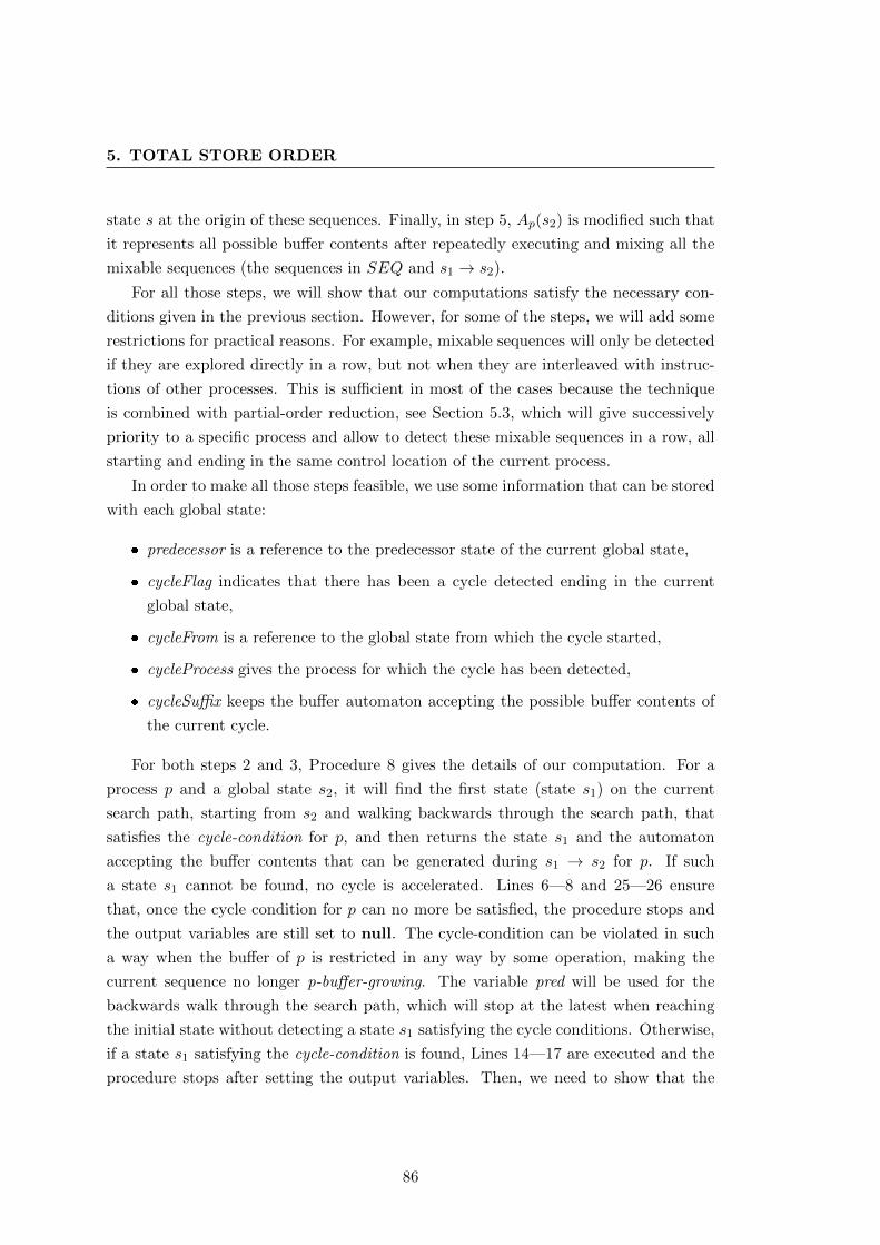
5. TOTAL STORE ORDER
state s at the origin of these sequences. Finally, in step 5, Ap(s2) is modified such that
it represents all possible buffer contents after repeatedly executing and mixing all the
mixable sequences (the sequences in SEQ and s1 → s2).
For all those steps, we will show that our computations satisfy the necessary con-
ditions given in the previous section. However, for some of the steps, we will add some
restrictions for practical reasons. For example, mixable sequences will only be detected
if they are explored directly in a row, but not when they are interleaved with instruc-
tions of other processes. This is sufficient in most of the cases because the technique
is combined with partial-order reduction, see Section 5.3, which will give successively
priority to a specific process and allow to detect these mixable sequences in a row, all
starting and ending in the same control location of the current process.
In order to make all those steps feasible, we use some information that can be stored
with each global state:
predecessor is a reference to the predecessor state of the current global state,
cycleFlag indicates that there has been a cycle detected ending in the current
global state,
cycleFrom is a reference to the global state from which the cycle started,
cycleProcess gives the process for which the cycle has been detected,
cycleSuffix keeps the buffer automaton accepting the possible buffer contents of
the current cycle.
For both steps 2 and 3, Procedure 8 gives the details of our computation. For a
process p and a global state s2, it will find the first state (state s1) on the current
search path, starting from s2 and walking backwards through the search path, that
satisfies the cycle-condition for p, and then returns the state s1 and the automaton
accepting the buffer contents that can be generated during s1 → s2 for p. If such
a state s1 cannot be found, no cycle is accelerated. Lines 6—8 and 25—26 ensure
that, once the cycle condition for p can no more be satisfied, the procedure stops and
the output variables are still set to null. The cycle-condition can be violated in such
a way when the buffer of p is restricted in any way by some operation, making the
current sequence no longer p-buffer-growing. The variable pred will be used for the
backwards walk through the search path, which will stop at the latest when reaching
the initial state without detecting a state s1 satisfying the cycle conditions. Otherwise,
if a state s1 satisfying the cycle-condition is found, Lines 14—17 are executed and the
procedure stops after setting the output variables. Then, we need to show that the
86
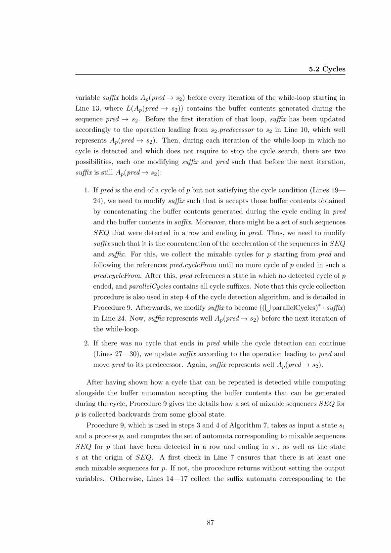
5.2 Cycles
variable suffix holds Ap(pred→ s2) before every iteration of the while-loop starting in
Line 13, where L(Ap(pred → s2)) contains the buffer contents generated during the
sequence pred → s2. Before the first iteration of that loop, suffix has been updated
accordingly to the operation leading from s2.predecessor to s2 in Line 10, which well
represents Ap(pred → s2). Then, during each iteration of the while-loop in which no
cycle is detected and which does not require to stop the cycle search, there are two
possibilities, each one modifying suffix and pred such that before the next iteration,
suffix is still Ap(pred→ s2):
1. If pred is the end of a cycle of p but not satisfying the cycle condition (Lines 19—
24), we need to modify suffix such that is accepts those buffer contents obtained
by concatenating the buffer contents generated during the cycle ending in pred
and the buffer contents in suffix. Moreover, there might be a set of such sequences
SEQ that were detected in a row and ending in pred. Thus, we need to modify
suffix such that it is the concatenation of the acceleration of the sequences in SEQ
and suffix. For this, we collect the mixable cycles for p starting from pred and
following the references pred.cycleFrom until no more cycle of p ended in such a
pred.cycleFrom. After this, pred references a state in which no detected cycle of p
ended, and parallelCycles contains all cycle suffixes. Note that this cycle collection
procedure is also used in step 4 of the cycle detection algorithm, and is detailed in
Procedure 9. Afterwards, we modify suffix to become ((⋃
parallelCycles)∗ · suffix)
in Line 24. Now, suffix represents well Ap(pred→ s2) before the next iteration of
the while-loop.
2. If there was no cycle that ends in pred while the cycle detection can continue
(Lines 27—30), we update suffix according to the operation leading to pred and
move pred to its predecessor. Again, suffix represents well Ap(pred→ s2).
After having shown how a cycle that can be repeated is detected while computing
alongside the buffer automaton accepting the buffer contents that can be generated
during the cycle, Procedure 9 gives the details how a set of mixable sequences SEQ for
p is collected backwards from some global state.
Procedure 9, which is used in steps 3 and 4 of Algorithm 7, takes as input a state s1
and a process p, and computes the set of automata corresponding to mixable sequences
SEQ for p that have been detected in a row and ending in s1, as well as the state
s at the origin of SEQ. A first check in Line 7 ensures that there is at least one
such mixable sequences for p. If not, the procedure returns without setting the output
variables. Otherwise, Lines 14—17 collect the suffix automata corresponding to the
87
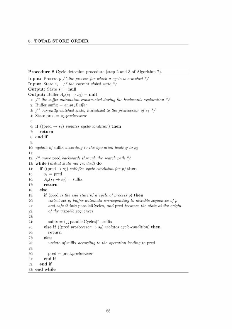
5. TOTAL STORE ORDER
Procedure 8 Cycle detection procedure (step 2 and 3 of Algorithm 7).
Input: Process p /* the process for which a cycle is searched */Input: State s2 /* the current global state */Output: State s1 = nullOutput: Buffer Ap(s1 → s2) = null
1: /* the suffix automaton constructed during the backwards exploration */2: Buffer suffix = emptyBuffer3: /* currently watched state, initialized to the predecessor of s2 */4: State pred = s2.predecessor5:
6: if ((pred → s2) violates cycle-condition) then7: return8: end if9:
10: update of suffix according to the operation leading to s211:
12: /* move pred backwards through the search path */13: while (initial state not reached) do14: if ((pred → s2) satisfies cycle-condition for p) then15: s1 = pred16: Ap(s1 → s2) = suffix17: return18: else19: if (pred is the end state of a cycle of process p) then20: collect set of buffer automata corresponding to mixable sequences of p21: and safe it into parallelCycles, and pred becomes the state at the origin22: of the mixable sequences23:
24: suffix = (⋃
parallelCycles)∗ · suffix25: else if ((pred.predecessor → s2) violates cycle-condition) then26: return27: else28: update of suffix according to the operation leading to pred29:
30: pred = pred.predecessor31: end if32: end if33: end while
88
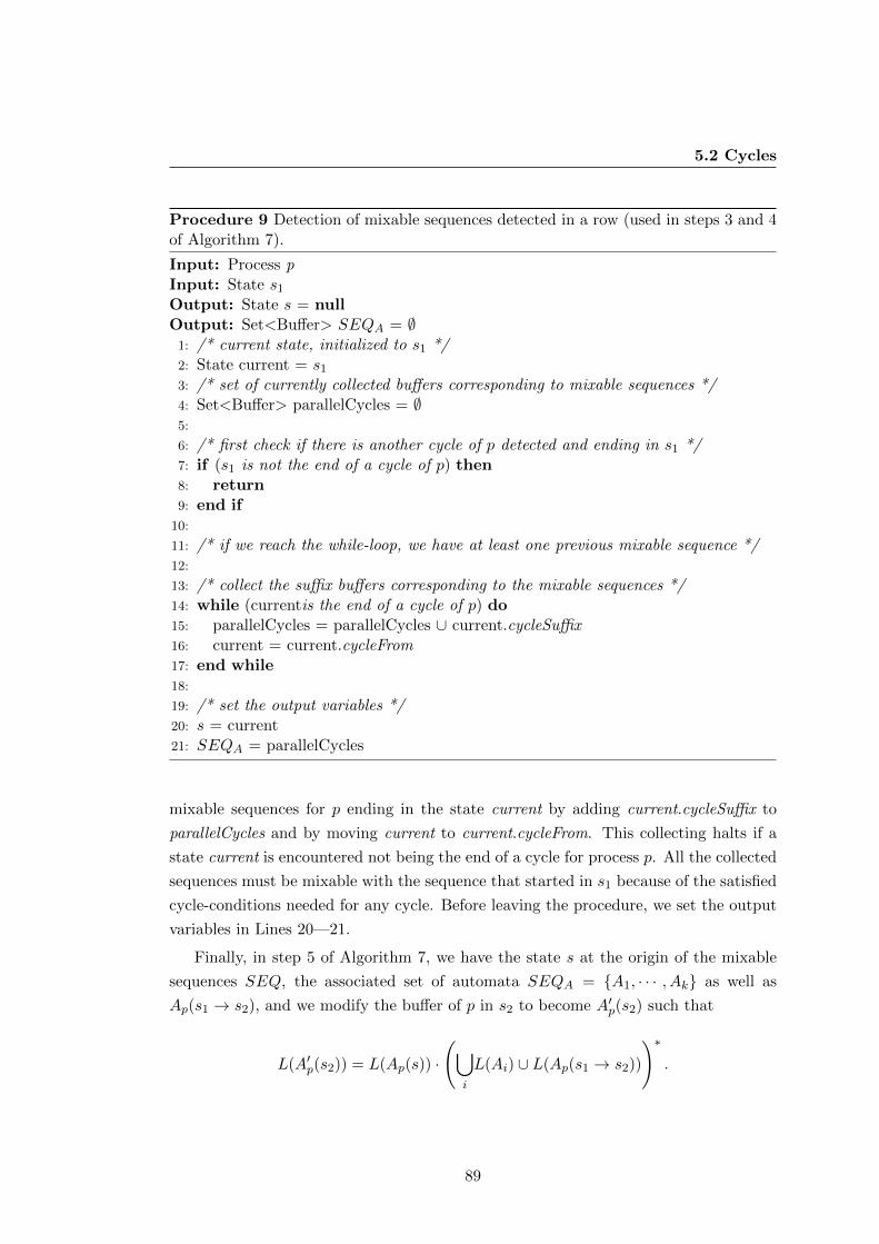
5.2 Cycles
Procedure 9 Detection of mixable sequences detected in a row (used in steps 3 and 4of Algorithm 7).
Input: Process pInput: State s1Output: State s = nullOutput: Set<Buffer> SEQA = ∅
1: /* current state, initialized to s1 */2: State current = s13: /* set of currently collected buffers corresponding to mixable sequences */4: Set<Buffer> parallelCycles = ∅5:
6: /* first check if there is another cycle of p detected and ending in s1 */7: if (s1 is not the end of a cycle of p) then8: return9: end if
10:
11: /* if we reach the while-loop, we have at least one previous mixable sequence */12:
13: /* collect the suffix buffers corresponding to the mixable sequences */14: while (currentis the end of a cycle of p) do15: parallelCycles = parallelCycles ∪ current.cycleSuffix16: current = current.cycleFrom17: end while18:
19: /* set the output variables */20: s = current21: SEQA = parallelCycles
mixable sequences for p ending in the state current by adding current.cycleSuffix to
parallelCycles and by moving current to current.cycleFrom. This collecting halts if a
state current is encountered not being the end of a cycle for process p. All the collected
sequences must be mixable with the sequence that started in s1 because of the satisfied
cycle-conditions needed for any cycle. Before leaving the procedure, we set the output
variables in Lines 20—21.
Finally, in step 5 of Algorithm 7, we have the state s at the origin of the mixable
sequences SEQ, the associated set of automata SEQA = A1, · · · , Ak as well as
Ap(s1 → s2), and we modify the buffer of p in s2 to become A′p(s2) such that
L(A′p(s2)) = L(Ap(s)) ·
(⋃i
L(Ai) ∪ L(Ap(s1 → s2))
)∗.
89
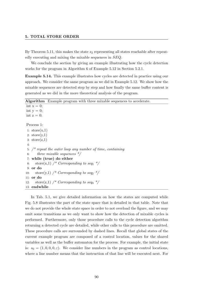
5. TOTAL STORE ORDER
By Theorem 5.11, this makes the state s2 representing all states reachable after repeat-
edly executing and mixing the mixable sequences in SEQ.
We conclude the section by giving an example illustrating how the cycle detection
works for the program in Algorithm 6 of Example 5.12 in Section 5.2.1.
Example 5.14. This example illustrates how cycles are detected in practice using our
approach. We consider the same program as we did in Example 5.12. We show how the
mixable sequences are detected step by step and how finally the same buffer content is
generated as we did in the more theoretical analysis of the program.
Algorithm Example program with three mixable sequences to accelerate.
int x = 0;int y = 0;int z = 0;
Process 1:
1: store(x,1)2: store(y,1)3: store(z,1)4:
5: /* repeat the outer loop any number of time, containing6: three mixable sequences */7: while (true) do either8: store(x,1) /* Corresponding to seq1 */9: or do
10: store(y,1) /* Corresponding to seq2 */11: or do12: store(z,1) /* Corresponding to seq3 */13: endwhile
In Tab. 5.1, we give detailed information on how the states are computed while
Fig. 5.8 illustrates the part of the state space that is detailed in that table. Note that
we do not provide the whole state space in order to not overload the figure, and we may
omit some transitions as we only want to show how the detection of mixable cycles is
performed. Furthermore, only those procedure calls to the cycle detection algorithm
returning a detected cycle are detailed, while other calls to this procedure are omitted.
These procedure calls are surrounded by dashed lines. Recall that global states of the
current example program are composed of a control location, values for the shared
variables as well as the buffer automaton for the process. For example, the initial state
is: s0 = (1, 0, 0, 0, ε). We consider line numbers in the program as control locations,
where a line number means that the instruction of that line will be executed next. For
90
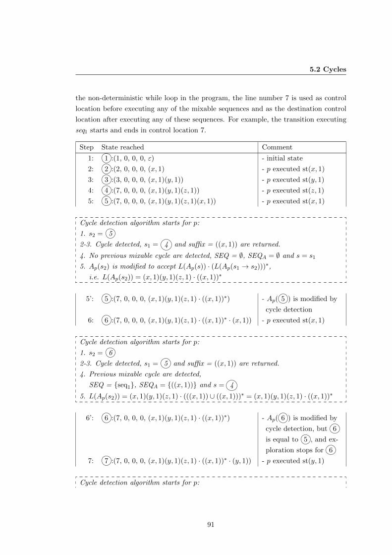
5.2 Cycles
the non-deterministic while loop in the program, the line number 7 is used as control
location before executing any of the mixable sequences and as the destination control
location after executing any of these sequences. For example, the transition executing
seq1 starts and ends in control location 7.
Step State reached Comment
1: 1 :(1, 0, 0, 0, ε) - initial state
2: 2 :(2, 0, 0, 0, (x, 1) - p executed st(x, 1)
3: 3 :(3, 0, 0, 0, (x, 1)(y, 1)) - p executed st(y, 1)
4: 4 :(7, 0, 0, 0, (x, 1)(y, 1)(z, 1)) - p executed st(z, 1)
5: 5 :(7, 0, 0, 0, (x, 1)(y, 1)(z, 1)(x, 1)) - p executed st(x, 1)
Cycle detection algorithm starts for p:
1. s2 = 5
2-3. Cycle detected, s1 = 4 and suffix = ((x, 1)) are returned.
4. No previous mixable cycle are detected, SEQ = ∅, SEQA = ∅ and s = s1
5. Ap(s2) is modified to accept L(Ap(s)) · (L(Ap(s1 → s2)))∗,
i.e. L(Ap(s2)) = (x, 1)(y, 1)(z, 1) · ((x, 1))∗
5’: 5 :(7, 0, 0, 0, (x, 1)(y, 1)(z, 1) · ((x, 1))∗) - Ap( 5 ) is modified by
cycle detection
6: 6 :(7, 0, 0, 0, (x, 1)(y, 1)(z, 1) · ((x, 1))∗ · (x, 1)) - p executed st(x, 1)
Cycle detection algorithm starts for p:
1. s2 = 6
2-3. Cycle detected, s1 = 5 and suffix = ((x, 1)) are returned.
4. Previous mixable cycle are detected,
SEQ = seq1, SEQA = ((x, 1)) and s = 4
5. L(Ap(s2)) = (x, 1)(y, 1)(z, 1) · (((x, 1)) ∪ ((x, 1)))∗ = (x, 1)(y, 1)(z, 1) · ((x, 1))∗
6’: 6 :(7, 0, 0, 0, (x, 1)(y, 1)(z, 1) · ((x, 1))∗) - Ap( 6 ) is modified by
cycle detection, but 6
is equal to 5 , and ex-
ploration stops for 6
7: 7 :(7, 0, 0, 0, (x, 1)(y, 1)(z, 1) · ((x, 1))∗ · (y, 1)) - p executed st(y, 1)
Cycle detection algorithm starts for p:
91
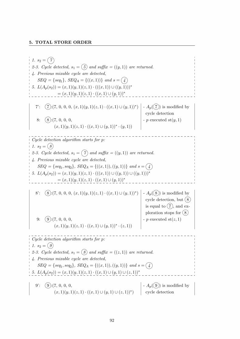
5. TOTAL STORE ORDER
1. s2 = 7
2-3. Cycle detected, s1 = 5 and suffix = ((y, 1)) are returned.
4. Previous mixable cycle are detected,
SEQ = seq1, SEQA = ((x, 1)) and s = 4
5. L(Ap(s2)) = (x, 1)(y, 1)(z, 1) · (((x, 1)) ∪ ((y, 1)))∗
= (x, 1)(y, 1)(z, 1) · ((x, 1) ∪ (y, 1))∗
7’: 7 :(7, 0, 0, 0, (x, 1)(y, 1)(z, 1) · ((x, 1) ∪ (y, 1))∗) - Ap( 7 ) is modified by
cycle detection
8: 8 :(7, 0, 0, 0, - p executed st(y, 1)
(x, 1)(y, 1)(z, 1) · ((x, 1) ∪ (y, 1))∗ · (y, 1))
Cycle detection algorithm starts for p:
1. s2 = 8
2-3. Cycle detected, s1 = 7 and suffix = ((y, 1)) are returned.
4. Previous mixable cycle are detected,
SEQ = seq1, seq2, SEQA = ((x, 1)), ((y, 1)) and s = 4
5. L(Ap(s2)) = (x, 1)(y, 1)(z, 1) · (((x, 1)) ∪ ((y, 1)) ∪ ((y, 1)))∗
= (x, 1)(y, 1)(z, 1) · ((x, 1) ∪ (y, 1))∗
8’: 8 :(7, 0, 0, 0, (x, 1)(y, 1)(z, 1) · ((x, 1) ∪ (y, 1))∗) - Ap( 8 ) is modified by
cycle detection, but 8
is equal to 7 , and ex-
ploration stops for 8
9: 9 :(7, 0, 0, 0, - p executed st(z, 1)
(x, 1)(y, 1)(z, 1) · ((x, 1) ∪ (y, 1))∗ · (z, 1))
Cycle detection algorithm starts for p:
1. s2 = 9
2-3. Cycle detected, s1 = 8 and suffix = ((z, 1)) are returned.
4. Previous mixable cycle are detected,
SEQ = seq1, seq2, SEQA = ((x, 1)), ((y, 1)) and s = 4
5. L(Ap(s2)) = (x, 1)(y, 1)(z, 1) · ((x, 1) ∪ (y, 1) ∪ (z, 1))∗
9’: 9 :(7, 0, 0, 0, - Ap( 9 ) is modified by
(x, 1)(y, 1)(z, 1) · ((x, 1) ∪ (y, 1) ∪ (z, 1))∗) cycle detection
92
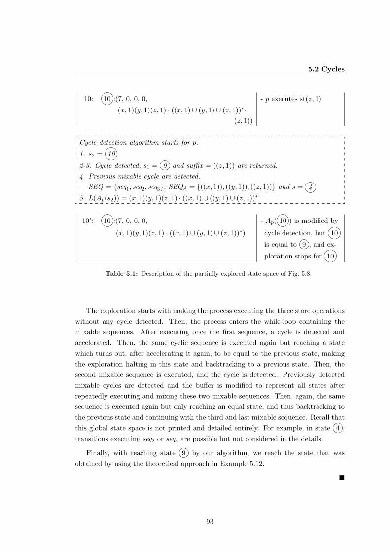
5.2 Cycles
10: 10 :(7, 0, 0, 0, - p executes st(z, 1)
(x, 1)(y, 1)(z, 1) · ((x, 1) ∪ (y, 1) ∪ (z, 1))∗·(z, 1))
Cycle detection algorithm starts for p:
1. s2 = 10
2-3. Cycle detected, s1 = 9 and suffix = ((z, 1)) are returned.
4. Previous mixable cycle are detected,
SEQ = seq1, seq2, seq3, SEQA = ((x, 1)), ((y, 1)), ((z, 1)) and s = 4
5. L(Ap(s2)) = (x, 1)(y, 1)(z, 1) · ((x, 1) ∪ ((y, 1) ∪ (z, 1))∗
10’: 10 :(7, 0, 0, 0, - Ap( 10 ) is modified by
(x, 1)(y, 1)(z, 1) · ((x, 1) ∪ (y, 1) ∪ (z, 1))∗) cycle detection, but 10
is equal to 9 , and ex-
ploration stops for 10
Table 5.1: Description of the partially explored state space of Fig. 5.8.
The exploration starts with making the process executing the three store operations
without any cycle detected. Then, the process enters the while-loop containing the
mixable sequences. After executing once the first sequence, a cycle is detected and
accelerated. Then, the same cyclic sequence is executed again but reaching a state
which turns out, after accelerating it again, to be equal to the previous state, making
the exploration halting in this state and backtracking to a previous state. Then, the
second mixable sequence is executed, and the cycle is detected. Previously detected
mixable cycles are detected and the buffer is modified to represent all states after
repeatedly executing and mixing these two mixable sequences. Then, again, the same
sequence is executed again but only reaching an equal state, and thus backtracking to
the previous state and continuing with the third and last mixable sequence. Recall that
this global state space is not printed and detailed entirely. For example, in state 4 ,
transitions executing seq2 or seq3 are possible but not considered in the details.
Finally, with reaching state 9 by our algorithm, we reach the state that was
obtained by using the theoretical approach in Example 5.12.
93
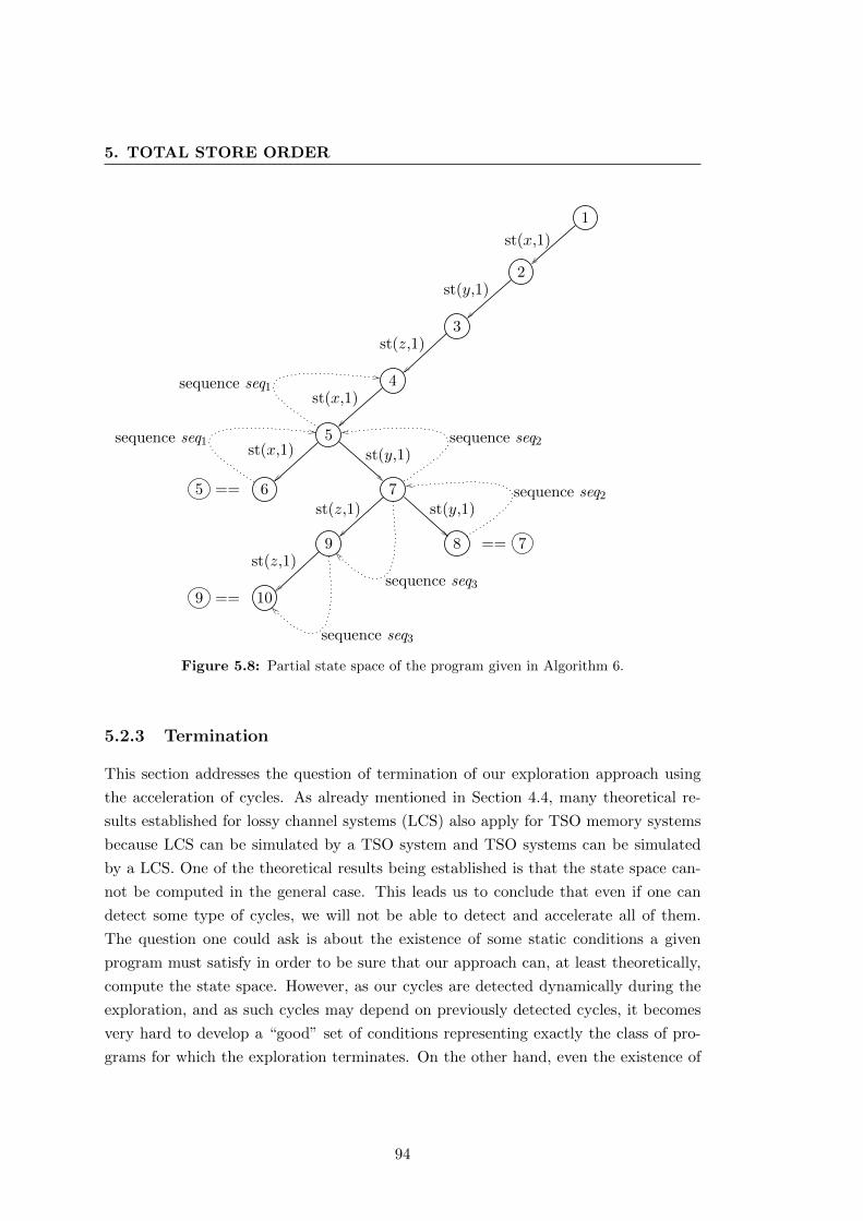
5. TOTAL STORE ORDER
st(x,1)
st(z,1)
st(x,1)
st(z,1)
st(z,1)
1
2
3
4
5
6 7
9
10
8
st(y,1)
st(y,1)
5 ==
9 ==
st(y,1)
st(x,1)sequence seq1
sequence seq1 sequence seq2
sequence seq2
== 7
sequence seq3
sequence seq3
Figure 5.8: Partial state space of the program given in Algorithm 6.
5.2.3 Termination
This section addresses the question of termination of our exploration approach using
the acceleration of cycles. As already mentioned in Section 4.4, many theoretical re-
sults established for lossy channel systems (LCS) also apply for TSO memory systems
because LCS can be simulated by a TSO system and TSO systems can be simulated
by a LCS. One of the theoretical results being established is that the state space can-
not be computed in the general case. This leads us to conclude that even if one can
detect some type of cycles, we will not be able to detect and accelerate all of them.
The question one could ask is about the existence of some static conditions a given
program must satisfy in order to be sure that our approach can, at least theoretically,
compute the state space. However, as our cycles are detected dynamically during the
exploration, and as such cycles may depend on previously detected cycles, it becomes
very hard to develop a “good” set of conditions representing exactly the class of pro-
grams for which the exploration terminates. On the other hand, even the existence of
94
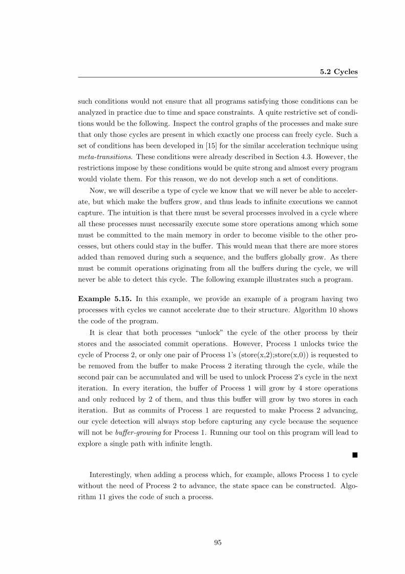
5.2 Cycles
such conditions would not ensure that all programs satisfying those conditions can be
analyzed in practice due to time and space constraints. A quite restrictive set of condi-
tions would be the following. Inspect the control graphs of the processes and make sure
that only those cycles are present in which exactly one process can freely cycle. Such a
set of conditions has been developed in [15] for the similar acceleration technique using
meta-transitions. These conditions were already described in Section 4.3. However, the
restrictions impose by these conditions would be quite strong and almost every program
would violate them. For this reason, we do not develop such a set of conditions.
Now, we will describe a type of cycle we know that we will never be able to acceler-
ate, but which make the buffers grow, and thus leads to infinite executions we cannot
capture. The intuition is that there must be several processes involved in a cycle where
all these processes must necessarily execute some store operations among which some
must be committed to the main memory in order to become visible to the other pro-
cesses, but others could stay in the buffer. This would mean that there are more stores
added than removed during such a sequence, and the buffers globally grow. As there
must be commit operations originating from all the buffers during the cycle, we will
never be able to detect this cycle. The following example illustrates such a program.
Example 5.15. In this example, we provide an example of a program having two
processes with cycles we cannot accelerate due to their structure. Algorithm 10 shows
the code of the program.
It is clear that both processes “unlock” the cycle of the other process by their
stores and the associated commit operations. However, Process 1 unlocks twice the
cycle of Process 2, or only one pair of Process 1’s (store(x,2);store(x,0)) is requested to
be removed from the buffer to make Process 2 iterating through the cycle, while the
second pair can be accumulated and will be used to unlock Process 2’s cycle in the next
iteration. In every iteration, the buffer of Process 1 will grow by 4 store operations
and only reduced by 2 of them, and thus this buffer will grow by two stores in each
iteration. But as commits of Process 1 are requested to make Process 2 advancing,
our cycle detection will always stop before capturing any cycle because the sequence
will not be buffer-growing for Process 1. Running our tool on this program will lead to
explore a single path with infinite length.
Interestingly, when adding a process which, for example, allows Process 1 to cycle
without the need of Process 2 to advance, the state space can be constructed. Algo-
rithm 11 gives the code of such a process.
95
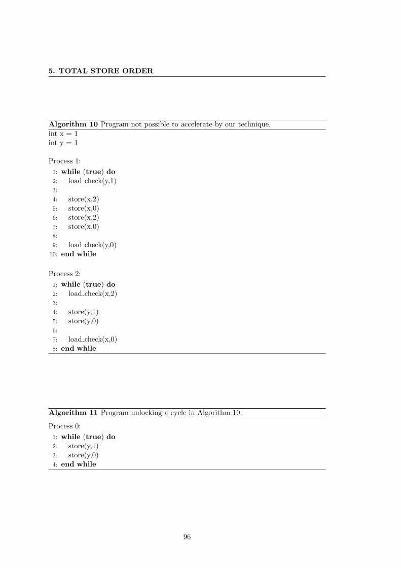
5. TOTAL STORE ORDER
Algorithm 10 Program not possible to accelerate by our technique.
int x = 1int y = 1
Process 1:
1: while (true) do2: load check(y,1)3:
4: store(x,2)5: store(x,0)6: store(x,2)7: store(x,0)8:
9: load check(y,0)10: end while
Process 2:
1: while (true) do2: load check(x,2)3:
4: store(y,1)5: store(y,0)6:
7: load check(x,0)8: end while
Algorithm 11 Program unlocking a cycle in Algorithm 10.
Process 0:
1: while (true) do2: store(y,1)3: store(y,0)4: end while
96
5.3 Partial-Order Reduction
5.3 Partial-Order Reduction
In this Section, we precisely describe how the partial-order reduction techniques can be
exploited in the case of TSO. We start with giving the independence relation of pairs
of transitions. Afterwards, we detail how persistent-sets will be computed, followed by
the computation of the sleep-sets. In a last step, we will show that the partial-order
reduction can safely be combined with our cycle acceleration technique described in
the previous section.
5.3.1 Independence Relation
To correctly use partial-order reduction techniques, we must have an independence
relation for pairs of transitions, which is provided in this section with respect to TSO
and buffer automata. We separate the pairs of transitions in two types: (1) pairs of
transitions within different processes are active, and (2) pairs of transitions within the
same process is active.
Before providing the pairs of independent transitions, recall the definition of inde-
pendent transitions, given in Section 4.2.1.
Definition 4.1 (from Section 4.2.1) Let T be the set of transitions in a concurrent
system, and D ⊆ T × T be a binary, reflexive and symmetric relation. The relation
D is a valid dependence relation for a concurrent system if and only if for all t1, t2 ∈T , (t1, t2) /∈ D (t1 and t2 are independent) implies that the two following properties hold
for all global states s of the state space of the concurrent system:
1. if t1 is enabled in s and st1→ s1, then t2 is enabled in s if and only if t2 is enabled
in s1 (independent transitions can neither disable nor enable each other); and
2. if t1 and t2 are enabled in s, then there is a unique state s′ such that st1→ s1
t2→ s′
and st2→ s2
t1→ s′ (commutativity of enabled independent transitions).
Also remember that as these conditions are not always easy to check, we gave
sufficient conditions for two transitions t1 and t2 to be independent in Section 4.2.1:
1. the set of processes that are active for t1 is disjoint from the set of processes that
are active for t2, and
2. the set of shared objects that are accessed by t1 is disjoint from the set of shared
objects that are accessed by t2.
97
5. TOTAL STORE ORDER
By adding the buffer-emptying process to our system in Section 5.1.9, we simplify
the definition of the independence relation for the pairs formed of a transition executing
a commit and transitions executing an operation of a process. Indeed, in this setting,
the active process is different when a transition executes an operation of a process or a
commit operation.
Note that we only specify those pairs of transitions that are independent, because
we only make use of these pairs. All other possible pairs are considered to be dependent.
5.3.1.1 Transitions of the Same Process
Pairings of transitions in which the same process p ∈ P is active are in most of the cases
dependent. The first condition of the sufficient syntactic conditions for independence
of two transitions is: the set of processes that are active for transition t1 is disjoint
from the set of processes that are active for transition t2. This is due to the fact that if
a transition is executed, the active process has moved, in most of the cases, to another
control location in which other outgoing transitions are possible than those in the
control location before executing that transition. Thus, we will consider these pairs of
transitions to be dependent. However, there exists one exception: pairs of transitions
in which the buffer-emptying process is active. Indeed, as this process only has one
control location, choosing a commit accessing Ap does not, for example, disable (or
enable) any commit on Ap′ with p 6= p′, and we need to inspect closely these pairs of
transitions.
Remark 5.16. In the following, when writing for example “A store transition t of
process p”, we mean “A transition t executing a store operation where process p is
active”. Moreover, the active process for any transition executing a commit operation
is pb.
The first pair of interesting transitions are those where both transitions execute
commit operations accessing different buffer automata, and both transitions update
different memory locations or the same memory location with the same value. In this
case, both transitions are considered to be independent. We have the following lemma.
Lemma 5.17. Let t1 be a commit transition accessing buffer b and t2 be a commit
transition accessing buffer b′. If t1 and t2 either access different memory locations
or both update the same memory location with the same value, then t1 and t2 are
independent.
Proof. We prove this by the formal definition of independent transitions. Let c1 be
the operation executed in t1, and c2 be the operation executed in t2. It is clear that
98
5.3 Partial-Order Reduction
a commit operation accessing one buffer cannot enable or disable a commit operation
accessing another buffer, and thus the first condition is satisfied. By the conditions
of the lemma, both c1 and c2 update either different memory locations or the same
location with the same value, hence executing the sequence t1,t2 or t2,t1 from a state
s in which both are enabled lead to the same state. In this state, both buffers have
executed their commit and where either both memory locations are updated in the same
way, and thus the second condition of the formal independence definition is satisfied as
well. The transitions t1 and t2 are thus independent.
A second pair of interesting transitions executing commit operations is when both
commits access the same buffer automaton when this automaton accepts words of the
following language
((
seq1︷︸︸︷α ) ∪ (
seq2︷︸︸︷β ) ∪ · · · )∗ · L1, where L1 ⊆ Σ∗, (5.2)
where α and β are the buffer elements to be transfered to memory by the actual
commit operations, and where Σ is the buffer alphabet. Such a form can be obtained
by accelerating a program close to Algorithm 13, having several mixable sequences.
Lemma 5.18 establishes then independence of both commits.
Lemma 5.18. Let t1, t2 be commit transitions accessing the buffer of p. Let Ap be a
buffer automaton such that L(Ap)) is of the form following to Equation 5.2. Let c1
be the commit operation executed in t1 corresponding to α of Equation 5.2 and c2 be
the one executed in t2 corresponding to β of Equation 5.2. If Ap(s) is computed in the
context of the state-space exploration using the techniques of this thesis, then t1 and t2
are independent.
Proof. Let seq1 be the cycle in Ap containing α and seq2 be the cycle in Ap containing
β. By the conditions of the lemma, we know that all buffer contents in L(Ap) are those
that can be generated by the regular expression (α∪β∪· · · )∗ ·L1, where L1 ⊆ Σ∗, which
are these that are accepted by an automaton having a form like the one in Fig. 5.9.
By construction of the cycles (when using cycle acceleration), we know that c1 and
c2 access different memory locations (otherwise, such a structure could never have been
generated because of the load-equivalence relation during the cycle detection procedure).
Moreover, we know that both cannot enable or disable each other, and updating the
memory by the sequences t1, t2 or t2, t1 from a state s in which both are enabled must
thus lead to the same state. The transitions t1 and t2 are thus independent.
99
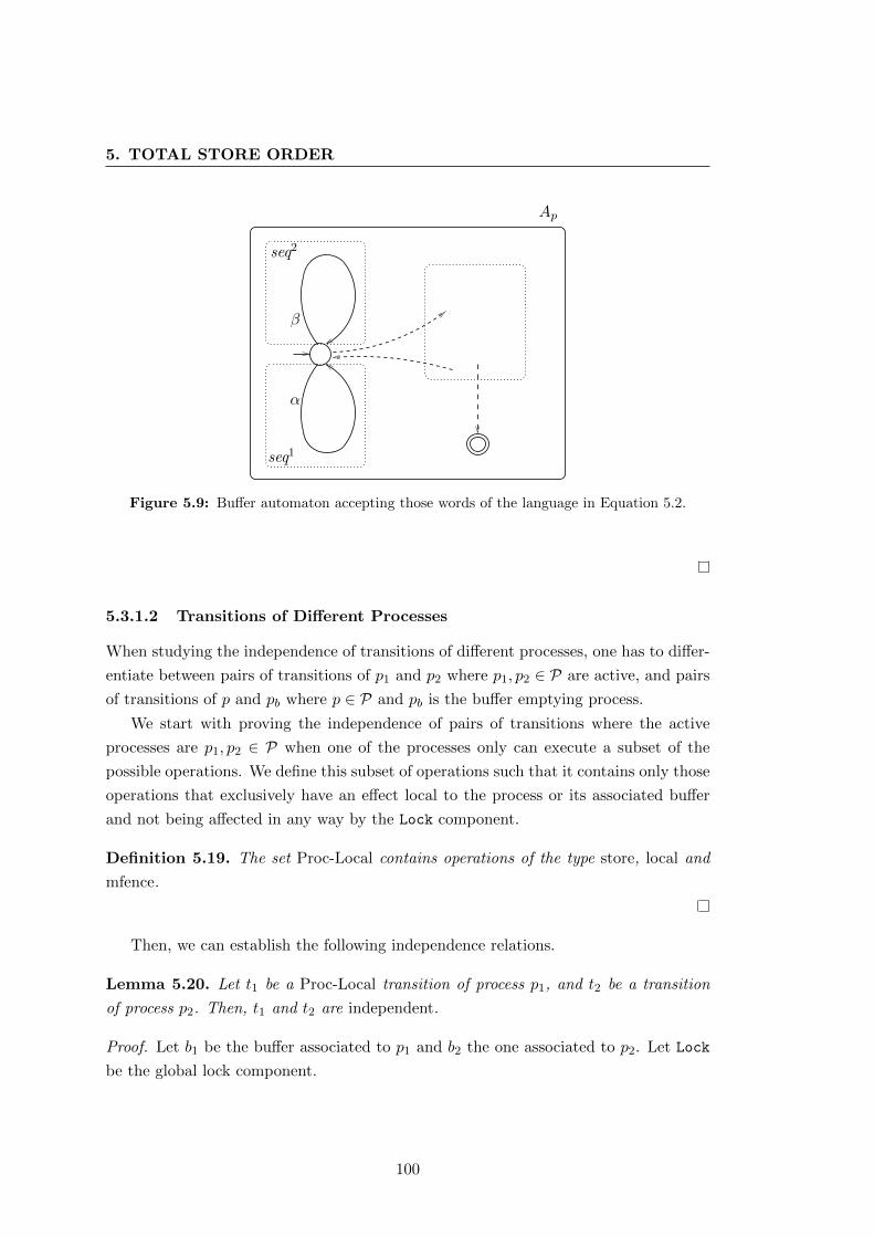
5. TOTAL STORE ORDER
β
seq2
Ap
seq1
α
Figure 5.9: Buffer automaton accepting those words of the language in Equation 5.2.
5.3.1.2 Transitions of Different Processes
When studying the independence of transitions of different processes, one has to differ-
entiate between pairs of transitions of p1 and p2 where p1, p2 ∈ P are active, and pairs
of transitions of p and pb where p ∈ P and pb is the buffer emptying process.
We start with proving the independence of pairs of transitions where the active
processes are p1, p2 ∈ P when one of the processes only can execute a subset of the
possible operations. We define this subset of operations such that it contains only those
operations that exclusively have an effect local to the process or its associated buffer
and not being affected in any way by the Lock component.
Definition 5.19. The set Proc-Local contains operations of the type store, local and
mfence.
Then, we can establish the following independence relations.
Lemma 5.20. Let t1 be a Proc-Local transition of process p1, and t2 be a transition
of process p2. Then, t1 and t2 are independent.
Proof. Let b1 be the buffer associated to p1 and b2 the one associated to p2. Let Lock
be the global lock component.
100
5.3 Partial-Order Reduction
Both syntactic conditions are satisfied. Indeed, the first condition is fulfilled directly
by the conditions of the lemma. The second condition is also satisfied, because the sets
of shared object that are effected is disjoint in both transitions. This might not be
clear, but as t1 only can access the local variables of p1 or the buffer b1 and is not
affected by the global lock, and t2 only can accesses the local variables of p2 or the
buffer b2 or Lock, the set of shared objects is empty, and we can conclude that these
transitions are independent.
We continue with establishing the independence of two loads executed by different
processes.
Lemma 5.21. If t1 is a load transition of p1 and if t2 is a load transition of p2, then
t1 and t2 are independent.
Proof. Indeed, both syntactic conditions are fulfilled: the active processes are different
in both operations by the conditions of the lemma, and the set of shared object is
disjoint.
The next pair of independent transitions is the one where both transitions execute
an unlock operation with different active processes.
Lemma 5.22. Let t1 be an unlock transition of p1, and t2 be an unlock transition of
p2. Then, t1 and t2 are independent.
Proof. The second condition of Definition 4.1 is trivially fulfilled because there doesn’t
exist a state s in which both are enabled. The first condition also holds. Suppose that
t1 executing unlock(p) is enabled in s. After executing this, t2 executing unlock(p′)
still cannot be enabled because to be enabled, p′ first needs to acquire the lock before
having the possibility to release it. It follows that those transitions are independent.
Note however that this independence will never lead to a reduction of the state space,
because there will never be any state in which both unlock transitions are enabled,
because only one process can hold the lock at a time.
We now consider a series of pairs of transitions where in one transition process
p ∈ P is active, and where in the second transition, the buffer emptying process pb is
active.
101
5. TOTAL STORE ORDER
Lemma 5.23. A local transition t1 of p is independent from a commit transition t2
(of pb).
Proof. By the syntactic conditions, t1 and t2 are independent because the active pro-
cesses are different, and because t1 does not access any shared object or buffer.
Lemma 5.24. A lock transition t1 of process p is independent from a commit transition
t2 accessing the buffer of p.
Proof. By the syntactic conditions, t1 and t2 are independent because the active pro-
cesses are different, and the two sets of shared objects used by them are disjoint.
Lemma 5.25. A store transition t1 of process p is independent from a commit tran-
sition t2 if both access the buffer automaton Ap and L(Ap) does not contain the empty
word.
Proof. Let st be the operation executed in t1, and let c be the operation executed in
t2. Let s be a state of the system. Let Σ be the alphabet of the buffer automaton,
let α ∈ Σ be the buffer element representing the store operation of st and β ∈ Σ
be the buffer element representing the buffered store operation to be committed by
c. By the condition of the lemma, we have L(Ap) ⊆ Σ+, or even more precisely
first(L(Ap)) · L1, where L1 ⊆ Σ∗. Thus, both st and c operate on different parts of the
buffer contents, the store only operates on the L1-part, while the commit only operates
on the “first(L(Ap))”-part.
The proof exploits the formal definition of independent transitions. As both st and
c operate on different parts of the buffer contents, they cannot enable or disable each
other, which makes the first condition fulfilled. The second condition also is fulfilled,
as both sequences t1, t2 and t2, t1 lead to the same state in case that both are enabled
in a state s. The first sequence first executes the store to reach a buffer automaton
accepting the words in the language first(L(Ap)) · L1 · α (where L1 ⊆ Σ∗) followed by
the commit leading to a buffer automaton accepting words of language L2 · α where
L2 ⊆ L1 is that part of L1 retained after executing the commit. The second sequence
first executes the commit to reach the buffer accepting the words in L2 ⊆ L1 followed
by executing the store to finally reach the buffer accepting the words in L2 · α, while
the restriction to the L1-part is equal the restriction in the first sequence. Both buffers
are thus equal after both sequences.
102
5.3 Partial-Order Reduction
Corollary 5.26. In state s, if a store transition t1 of process p and a commit transition
t2 are both enabled and accessing buffer automaton Ap, both transitions are independent.
Proof. This is a very similar to the proof of Lemma 5.25, and we only give the intuition:
both transitions being enabled in the state, and thus they operate on strictly different
parts of the same buffer, which implies that they cannot disable or enable each other
and both orders of execution will lead to the same state.
The following lemma is not aimed at proving any independence between a store and
a commit, but rather establishes that every possible commit emerges from a previously
executed store.
Lemma 5.27. In state s, if a store transition t1 of process p is enabled while the buffer
automaton Ap contains the empty word, only t1 can enable a commit transition t2 which
can transfer the buffer content corresponding to t1 from Ap to the shared memory.
Proof. This is immediate. Indeed, when the store operation adds the element (α) at the
end of each buffer content of L(Ap) to reach A′p such that L(A′p) = L(Ap) · α, then the
empty word in L(Ap) becomes α in L(A′p), and a commit becomes possible to transfer
α to the shared memory which was not possible before.
Lemma 5.28. In state s, if a store transition t1 of process p and a commit transition
t2 are both enabled while t1 accesses buffer b and t2 accesses buffer b′ with b 6= b′, then
t1 and t2 are independent.
Proof. This is immediate, because the active processes in both transition are different,
and as the set of shared objects are disjoint in both transitions.
Lemma 5.29. A load transition t1 on buffer Ap is independent from a commit tran-
sition t2 on the same buffer if both t1 and t2 are buffer-preserving.
For this to prove, we use the formal conditions of Definition 4.1.
Proof. Let ` be the load operation executed in t1, and let c be the commit operation
executed in t2. Let s be a state of the system in which both are possible to execute.
Let Σ be the alphabet of the buffer automaton, and let β ∈ Σ be the buffer element
representing the buffered store operation to be committed by c. Let A1p be the buffer
automaton after executing t1 from s. The conditions of the lemma tell us that both
103
5. TOTAL STORE ORDER
operations are buffer-preserving. For the load operation, this means that there is a
single value possible to load for the current variable (v), which is going to be loaded
from each buffer content in L(Ap), or from the shared memory which implies that no
buffer content of L(Ap) contains an element corresponding to a buffer store operation
to the variable in question. For the commit operation, it means that the function
first(L(Ap)) only returns a single value and ε /∈ L(Ap).
First, we need to prove the first condition: If t1 is enabled in s and st1→ s1, then
t2 is enabled in s if and only if t2 is enabled in s1. Indeed, as t1 does not modify the
buffer, both first(L(Ap)) and first(L(A1p)) return the same pair, β, to be committed.
Second, we need to prove the second condition: If t1 and t2 are enabled in s, then
there is a unique state s′ reached from s after executing either t1, t2 or t2, t1. In case
where the load operation does not load the value from the buffer element that is (or
will be) committed by t2, executing either first t1 or t2 and then t2 or t1 must lead to
the same state s′ because the load reads from another element of the buffer content
than from the first element, and because the commit only removes the first element
from each buffer content. In case that the load reads from the first element, the load
will read the value from the shared memory when the element is committed, and read
it from the buffer if not, and both sequences will lead to the same state.
We define the relation does-not-see between a load and a commit operation as
follows.
Definition 5.30. A load operation ` by process p does-not-see the effect of a commit
operation c on Ap′ if either ` only reads from Ap or if c writes to the memory location
that value that already locates in the location.
Lemma 5.31. A load transition t1 on buffer Ap (executing operation `) is independent
from a commit transition t2 (executing operation c) on buffer Ap′ if ` does-not-see the
effect of c.
Proof. This is directly proven by the syntactic conditions. First, the active processes in
both operations are different. Second, as the load does-not-see the effect of the commit,
it means that it can thus be considered as a no-op with respect to the memory and to
the load. It follows that the set of accessed objects is disjoint for both operations, and
the operations are independent.
104
5.3 Partial-Order Reduction
Next, we consider pairs of mfence and commit transitions. Among these, the only
dependent pair is when the mfence operation is buffer-modifying and removes some
buffer contents which then can not be committed any more, thus disabling forever the
corresponding commit(s).
Lemma 5.32. An mfence transition t1 of process p is independent from a commit
transition t2 accessing Ap if L(Ap) contains only the empty word.
Proof. Direct, as there can be no commit accessing Ap in s because the buffer is empty.
Lemma 5.33. An mfence transition t1 of process p is independent from a commit
transition t2 accessing Ap′.
Proof. This directly follows from the syntactic conditions. The first condition is fulfilled
because the active processes are different, and the second condition is fulfilled because
the sets of shared objects are disjoint.
Lemma 5.34. An unlock transition t1 of process p is independent from a commit
transition t2 accessing Ap if L(Ap) contains only the empty word.
Proof. Identical to proof of Lemma 5.32.
Remark 5.35. We did not inspect explicitly the pairing of a commit transitions and a
load check transitions. However, we did implicitly by inspecting the pairing of a commit
transition and a load transition. The analysis of the pairing commit and load check
when considering dependence is identical to the analysis of the pair (load, commit).
Indeed, a successfully executed load check operation is identical to a load operation in
which the requested value of the load check is loaded (and assigned to a local variable),
and both operations can be affected in the same way by a commit operation.
5.3.2 Persistent-Sets
In this section, we describe the way of the persistent-set computation. This computation
is independent from the property to check during the state-space exploration. However,
as we will see in a later chapter, such a property can influence which persistent-set to
select in a given state.
In a first step, we will recall the definition of a persistent-set [31], which we already
gave in Section 4.2.2 in Definition 4.2. Then, we will describe stubborn-sets [71] that
105
5. TOTAL STORE ORDER
were introduced before the notion of persistent-sets existed, but which fulfill the defi-
nition of persistent-sets, as it was shown in [31]. For these stubborn-sets, there exists
an algorithm computing such sets, which was given in [31] and which we will use in an
adapted form in order to compute our persistent-sets.
Recall Section 4.2.2 where persistent-sets were described. A set of transitions T
is persistent in a state s if any transition that is not in T is independent from the
transitions in T , and which can be defined as follows.
Definition 4.2 (from Section 4.2.2) A set T of transitions enabled in a state s is
persistent in s if and only if, for all nonempty sequences of transitions
s = s1t1→ s2
t2→ . . .tn−1→ sn
tn→ sn+1
from s in the state space and including only transitions ti /∈ T, 1 ≤ i ≤ n, tn is
independent in sn from all transitions in T .
Following to that, we give the definition of the stubborn-sets [71] which will allow
us to compute valid persistent-sets.
Definition 5.36. A set Ts of transitions is a stubborn-set in a state s if Ts contains
at least one enabled transition, and if for all transitions t ∈ Ts, the two following
conditions hold:
1. if t is disabled in s, then all transitions in one necessary enabling set NES(t,s)
for t in s are also in Ts;
2. if t is enabled in s, then all transitions t′ that “do-not-accord” with t are also in
Ts.
As a stubborn-set in some state s is proven to be a persistent-set in s, see [31],
we can use this algorithm for our persistent-set computation. This definition contains
two notations that we did not introduce formally. We will only give the ideas, but the
interested reader is redirected to [71] and [31] for further information. The set NES(t,s)
is a set of transitions for t in s, t being disabled in s, such that t cannot become enabled
from s without executing at least one transition of NES(t,s). Two transitions t1 and
t2 do-not-accord with each other if there exists a state in which they are both enabled
and dependent.
106
5.3 Partial-Order Reduction
We can now propose our algorithm for persistent-set computation, see Algorithm 12.
The idea of this algorithm is to look for a process for which only store or local operations
can be executed in the current state (enabled or disabled). When this is the case, we
chose the enabled transitions of this process to be the persistent-set. If such a process
cannot be found, we chose the persistent-set to be the set of enabled transitions of this
state.
Algorithm 12 Persistent-set computation in a state s.
1. Search for a process p in state s such that p only has transitions executing storeor local operations in the set of transitions to execute in s.
2. Then,
(a) if such a p can be found, let Ts be the enabled transitions of p in s,
(b) otherwise, chose Ts = enabled(s).
We now prove that Algorithm 12 always produces a set of transitions satisfying
Definition 5.36 to be a stubborn-set, and thus being a persistent-set.
Theorem 5.37. The sets of transitions computed by Algorithm 12 are persistent-sets.
Proof. Algorithm 12 can compute sets in two ways. In the first way, a subset of all
enabled transitions is computed, for which we will prove that this subset is indeed
a stubborn-set. In the second way, all enabled transitions are chosen to figure in
the persistent-set. In this case, the set is trivially persistent, as it was described in
Section 4.2.2.
For the first way of our persistent-set computation, we reason as follows. Let p be
the process such that p only has transitions to execute (from the current state s) that
execute either a store or a local operation. Let Ts be this set. Let bp be the buffer
associated to p in s. We show that Ts satisfies the definitions of stubborn-sets.
If t executes a store operation, we know that:
1. t is enabled in every case (a store operation that is possible to execute in a given
state is always enabled),
2. t is considered to be dependent with respect to all transitions of the same process,
3. t is independent from every transition of a different process p′ ∈ P (Lemma 5.20),
107
5. TOTAL STORE ORDER
4. t and the commit transition which transfers the buffer content corresponding to t
to the main memory are dependent. All other transitions executing other commit
operations are independent from t (Lemmas 5.25-5.28).
The first point leads us to only consider the condition 2 of Definition 5.36. The
second point highlights that all transitions of the same process must be added to the
persistent-set, which is systematically done in each persistent-set computation. Point
three shows that we do not need to add any transitions of other processes p′ ∈ P to
Ts. The last point does also not require to add any enabled commit operations to
Ts. Two types of commit transitions have to be considered. First, consider those that
accesses a different buffer than bp. By Lemma 5.28, we know that these commits are
independent from t of p. Second, we need to consider those commits accessing bp. By
Corollary 5.26, we know that each commit transition that is enabled in s and accessing
bp is independent from t, and no commit transitions need to be added. In case that a
commit transition t′ could be enabled by t, we know by Lemma 5.27 that only t can
enabled it. The set of transitions only containing t is then a valid set NES(t′, s). As
t is already present in the current persistent-set and as t′ is disabled, we need do not
need to add further transitions to the persistent-set.
In the case that t executes a local operation, all the conditions of Definition 5.36 are
also satisfied. In this case, we know the following about t:
1. t is enabled or disabled in s,
2. t is considered to be dependent with respect to all transitions of the same process,
3. t is independent from every transition of a process p′ 6= p with p′ ∈ P and from
every transition of process pb (Lemmas 5.20 and 5.23).
If t is enabled, then all transitions that do-not-accord with t belong to the same
process. As we have all transitions of the current process added to Ts, all operations
that do-not-accord are added and the first condition of a persistent-set is fulfilled. If t
is disabled, at least one transition required to make t enabled must be added. A local
transition that can be disabled must be some Boolean combination of local registers.
In order to allow these registers to be modified, a necessary condition is to make the
current process moving, because otherwise, the registers will never change. As we add
all transitions of the process to Ts, we provide all possible ways the registers to change,
consisting in a valid NES(t,s).
By proving that the set of transitions computed by our algorithm is either the set
of enabled transitions or a stubborn-set, we conclude that Algorithm 12 computes only
108
5.3 Partial-Order Reduction
persistent-sets.
5.3.3 Sleep-Sets
In this section, we describe the sleep-set computation in the context of TSO with respect
to global states that may symbolically represent a set of states. Remember that we
already introduced the concept of sleep-sets in Section 4.2.3. Recall that the intuition
behind sleep-sets is to avoid re-exploring states by different interleavings. A sleep-set is
associated to each global state, and represents transitions that are enabled in this state
but that will not be executed. However, it might happen that a state s is re-explored
a second time with a different sleep-set. This time, the transitions to follow are those
that are in the sleep-set of the corresponding state stored in the hash table but not in
the sleep-set of the current state s. Both the sleep-set of the current state and of the
state in the hash table must then be set to their intersection.
As in our approach, we do handle sets of states in a single global state, we need to
handle those cases in which a state s is visited and for which exists an already visited
state s′ such that s′ includes all states represented by s. For this, we need to adapt
the update-procedure of the sleep-sets in case that the currently visited state is equal
to an already visited state and/or included into one or several already visited states.
Lines 3—10 of Algorithm 5 are replaced by Procedure 13 for this purpose. Before we
can give this procedure, we need to define the concept of a state being included in
another state, which is given in Definition 5.38.
Definition 5.38. A state s1 is included in a state s2 if the following conditions are
satisfied:
∀p ∈ P : cp(s1) = cp(s2)
∀m ∈M : m(s1) = m(s2)
Lock(s1) = Lock(s2)
∀p ∈ P : L(Ap(s1)) ⊆ L(Ap(s2))
Thus, a state s1 is included in s2 if the set of states represented by s1 is included in
the set of states represented by s2. For this, all parts different from the store buffers
must be identical in both states, while the buffer contents in the corresponding store
buffers must satisfy the inclusion relation.
109
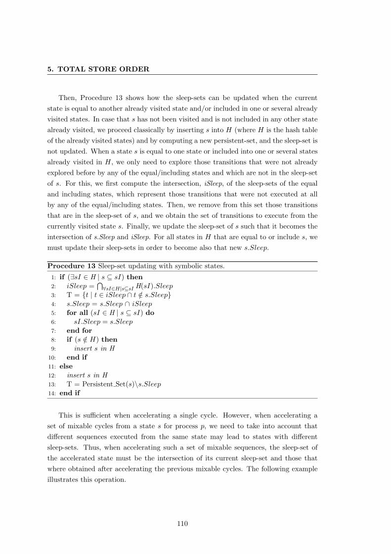
5. TOTAL STORE ORDER
Then, Procedure 13 shows how the sleep-sets can be updated when the current
state is equal to another already visited state and/or included in one or several already
visited states. In case that s has not been visited and is not included in any other state
already visited, we proceed classically by inserting s into H (where H is the hash table
of the already visited states) and by computing a new persistent-set, and the sleep-set is
not updated. When a state s is equal to one state or included into one or several states
already visited in H, we only need to explore those transitions that were not already
explored before by any of the equal/including states and which are not in the sleep-set
of s. For this, we first compute the intersection, iSleep, of the sleep-sets of the equal
and including states, which represent those transitions that were not executed at all
by any of the equal/including states. Then, we remove from this set those transitions
that are in the sleep-set of s, and we obtain the set of transitions to execute from the
currently visited state s. Finally, we update the sleep-set of s such that it becomes the
intersection of s.Sleep and iSleep. For all states in H that are equal to or include s, we
must update their sleep-sets in order to become also that new s.Sleep.
Procedure 13 Sleep-set updating with symbolic states.
1: if (∃sI ∈ H | s ⊆ sI) then2: iSleep =
⋂∀sI∈H|s⊆sI H(sI).Sleep
3: T = t | t ∈ iSleep ∩ t /∈ s.Sleep4: s.Sleep = s.Sleep ∩ iSleep5: for all (sI ∈ H | s ⊆ sI) do6: sI.Sleep = s.Sleep7: end for8: if (s /∈ H) then9: insert s in H
10: end if11: else12: insert s in H13: T = Persistent Set(s)\s.Sleep14: end if
This is sufficient when accelerating a single cycle. However, when accelerating a
set of mixable cycles from a state s for process p, we need to take into account that
different sequences executed from the same state may lead to states with different
sleep-sets. Thus, when accelerating such a set of mixable sequences, the sleep-set of
the accelerated state must be the intersection of its current sleep-set and those that
where obtained after accelerating the previous mixable cycles. The following example
illustrates this operation.
110
5.3 Partial-Order Reduction
Example 5.39. Let s be the state at the origin of a set of mixable sequences SEQ =
seq1, . . . , seqk for process p. Let s1 be the state after reached after accelerating
all these sequences except the last (seqk). Let s2 be the currently visited state af-
ter executing and accelerating this last sequence seqk. Then, the sleep-set becomes
s1.Sleep ∩ s2.Sleep.
By doing so, we ensure that the sequential acceleration of mixable sequences will
always lead to a state having a sleep-set that only contains those transitions that are
present in all the sleep-sets of the states that accelerated the different mixable sequences.
5.3.4 Depth-First Search by Combining Partial-Order Reduction and
Cycle Acceleration in TSO
This section is aimed at describing the power of combining our symbolic states with
partial-order reduction. First, the reason why cycles are detected quite fast in practice
is that the combination of persistent-sets and sleep-sets tries giving successively priority
to a given process, which makes it possible to detect quickly these “inner-process” cycles
we are looking for.
The second reason why the exploration is very effective is that the state space only
needs to be explored partially because of the selective search thanks to the basic use of
persistent-sets (and sleep-sets). Using our persistent-set computation, store and local
transitions are given priority over loads, commits and other operations. If such a set
can be found, only a few operations are selected to be executed (in most of the times,
there will only be one operation to execute), and only once no more fully independent
transitions are possible to be selected, loads and commits are grouped together and
executed block-wise.
The third reason resides in the combination of the cycles and the use of sleep-sets.
Indeed, the same cycle of a process can be detected from many different “global” states,
while the difference might only be a different control location of another process. In
these cases, the same cycle would be wastefully detected from each of these slightly
different global states without leading to new behaviors. The use of sleep-sets limits
this redetection of the same cycles. Consider a state s in which a cycle for process p
has already been accelerated (let seq be that cyclic sequence). Let t1 be a transition
in seq, and t2 be a transition of a different process, t1 and t2 being independent. Let
the persistent-set in s be t1, t2. When the exploration of the state space follows t1,
this transition will lead to a state where the exploration will stop (because this state
will be equal or included in a previously visited state). The exploration will return to
111
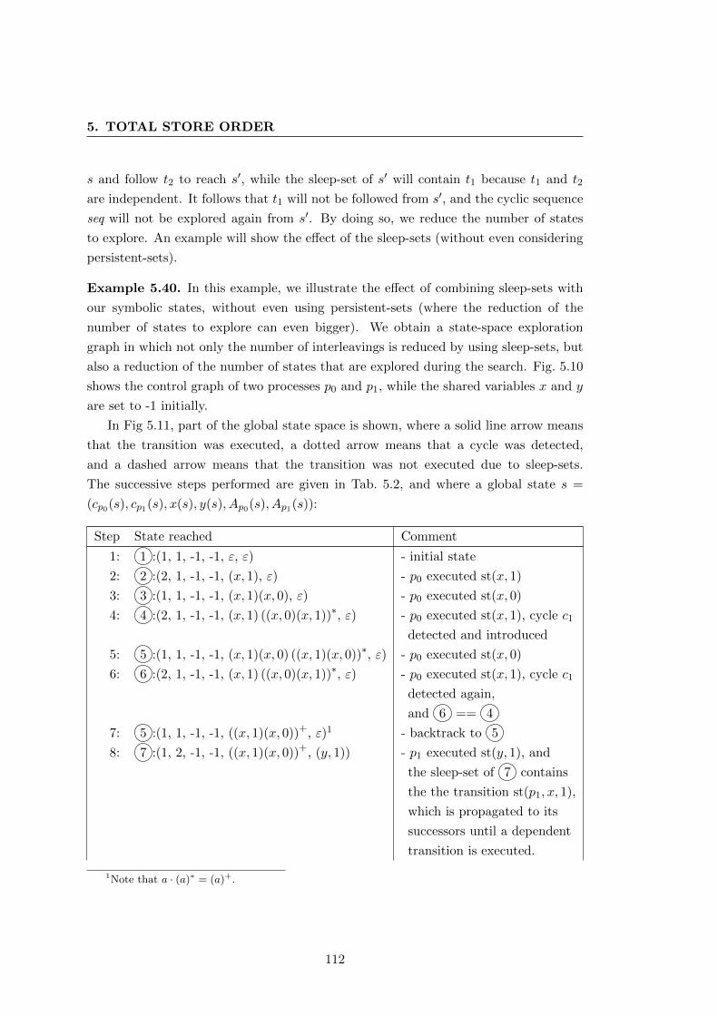
5. TOTAL STORE ORDER
s and follow t2 to reach s′, while the sleep-set of s′ will contain t1 because t1 and t2
are independent. It follows that t1 will not be followed from s′, and the cyclic sequence
seq will not be explored again from s′. By doing so, we reduce the number of states
to explore. An example will show the effect of the sleep-sets (without even considering
persistent-sets).
Example 5.40. In this example, we illustrate the effect of combining sleep-sets with
our symbolic states, without even using persistent-sets (where the reduction of the
number of states to explore can even bigger). We obtain a state-space exploration
graph in which not only the number of interleavings is reduced by using sleep-sets, but
also a reduction of the number of states that are explored during the search. Fig. 5.10
shows the control graph of two processes p0 and p1, while the shared variables x and y
are set to -1 initially.
In Fig 5.11, part of the global state space is shown, where a solid line arrow means
that the transition was executed, a dotted arrow means that a cycle was detected,
and a dashed arrow means that the transition was not executed due to sleep-sets.
The successive steps performed are given in Tab. 5.2, and where a global state s =
(cp0(s), cp1(s), x(s), y(s), Ap0(s), Ap1(s)):
Step State reached Comment
1: 1 :(1, 1, -1, -1, ε, ε) - initial state
2: 2 :(2, 1, -1, -1, (x, 1), ε) - p0 executed st(x, 1)
3: 3 :(1, 1, -1, -1, (x, 1)(x, 0), ε) - p0 executed st(x, 0)
4: 4 :(2, 1, -1, -1, (x, 1) ((x, 0)(x, 1))∗, ε) - p0 executed st(x, 1), cycle c1
detected and introduced
5: 5 :(1, 1, -1, -1, (x, 1)(x, 0) ((x, 1)(x, 0))∗, ε) - p0 executed st(x, 0)
6: 6 :(2, 1, -1, -1, (x, 1) ((x, 0)(x, 1))∗, ε) - p0 executed st(x, 1), cycle c1
detected again,
and 6 == 4
7: 5 :(1, 1, -1, -1, ((x, 1)(x, 0))+, ε)1 - backtrack to 5
8: 7 :(1, 2, -1, -1, ((x, 1)(x, 0))+, (y, 1)) - p1 executed st(y, 1), and
the sleep-set of 7 contains
the the transition st(p1, x, 1),
which is propagated to its
successors until a dependent
transition is executed.
1Note that a · (a)∗ = (a)+.
112
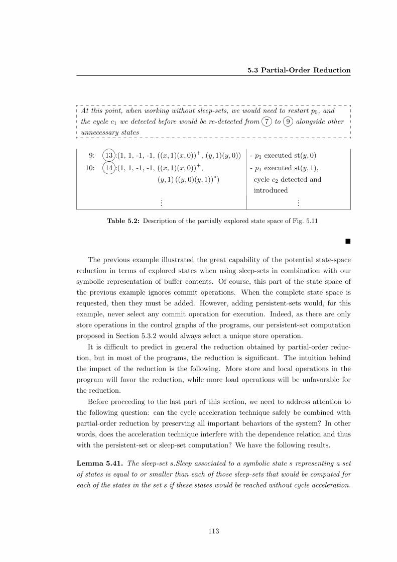
5.3 Partial-Order Reduction
At this point, when working without sleep-sets, we would need to restart p0, and
the cycle c1 we detected before would be re-detected from 7 to 9 alongside other
unnecessary states
9: 13 :(1, 1, -1, -1, ((x, 1)(x, 0))+, (y, 1)(y, 0)) - p1 executed st(y, 0)
10: 14 :(1, 1, -1, -1, ((x, 1)(x, 0))+, - p1 executed st(y, 1),
(y, 1) ((y, 0)(y, 1))∗) cycle c2 detected and
introduced...
...
Table 5.2: Description of the partially explored state space of Fig. 5.11
The previous example illustrated the great capability of the potential state-space
reduction in terms of explored states when using sleep-sets in combination with our
symbolic representation of buffer contents. Of course, this part of the state space of
the previous example ignores commit operations. When the complete state space is
requested, then they must be added. However, adding persistent-sets would, for this
example, never select any commit operation for execution. Indeed, as there are only
store operations in the control graphs of the programs, our persistent-set computation
proposed in Section 5.3.2 would always select a unique store operation.
It is difficult to predict in general the reduction obtained by partial-order reduc-
tion, but in most of the programs, the reduction is significant. The intuition behind
the impact of the reduction is the following. More store and local operations in the
program will favor the reduction, while more load operations will be unfavorable for
the reduction.
Before proceeding to the last part of this section, we need to address attention to
the following question: can the cycle acceleration technique safely be combined with
partial-order reduction by preserving all important behaviors of the system? In other
words, does the acceleration technique interfere with the dependence relation and thus
with the persistent-set or sleep-set computation? We have the following results.
Lemma 5.41. The sleep-set s.Sleep associated to a symbolic state s representing a set
of states is equal to or smaller than each of those sleep-sets that would be computed for
each of the states in the set s if these states would be reached without cycle acceleration.
113
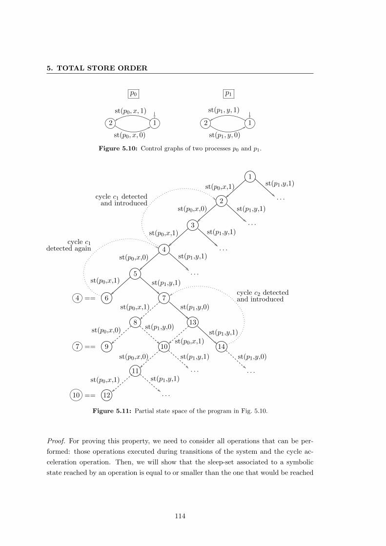
5. TOTAL STORE ORDER
12
st(p1, y, 0)
12
st(p0, x, 0)
st(p0, x, 1) st(p1, y, 1)
p0 p1
Figure 5.10: Control graphs of two processes p0 and p1.
st(p0,x,1)
st(p0,x,1)
st(p0,x,0)
st(p0,x,1)
st(p1,y,1)
st(p1,y,1)
st(p1,y,1)
st(p1,y,1)
· · ·
· · ·
· · ·
· · ·
st(p0,x,0)
st(p0,x,1)
· · ·
st(p1,y,1)· · ·
1
2
3
4
5
6 7
8
9 10
13
11
12
st(p1,y,1)
st(p1,y,0)
st(p0,x,0)
cycle c1 detectedand introduced
detected again
4 ==
7 ==
10 ==
14
· · ·
cycle c2 detectedand introduced
st(p0,x,0)
st(p0,x,1)
st(p1,y,1)
st(p0,x,1)st(p1,y,1)
st(p1,y,0)
st(p1,y,0)
cycle c1
Figure 5.11: Partial state space of the program in Fig. 5.10.
Proof. For proving this property, we need to consider all operations that can be per-
formed: those operations executed during transitions of the system and the cycle ac-
celeration operation. Then, we will show that the sleep-set associated to a symbolic
state reached by an operation is equal to or smaller than the one that would be reached
114
5.3 Partial-Order Reduction
when no cycle acceleration is used. First, consider the operation of acceleration. This
operation modifies the global state s to become the state representing all states after
repeatedly executing the current cyclic sequence that is accelerated by the current op-
eration. As we only detect cycles when they have been iterated at least one time, all
transitions that are dependent with respect to the transitions executed during the cycle
already disappeared from the sleep-set. This also holds when there exists previously
detected cycles that form a mixable set of sequences with the currently detected cycle
(remember that the sleep-set of the state after accelerating all these sequences is the
intersection of the sleep-sets of those states that are reached after executing one of these
sequences). Indeed, all the sequences have been executed at least one time and are exe-
cuted in a row without being interleaved by another transition, and thus all transitions
dependent with respect to one of transitions of these sequences have disappeared from
the sleep-set. Every repetition of any of the mixable sequences would not remove any
more transitions from the sleep-set. Then, we can conclude that the sleep-set of s is
identical to or smaller than the one of each state represented by s. Second, we need
to consider those operations executed by some transition. As our dependence relation
cares about the buffer contents accepted by the buffer automata, only those transitions
are preserved in the sleep-set that are independent from the current transition with
respect to all buffer contents accepted by the buffer automata. Otherwise, transitions
that may be dependent for some buffer contents will be removed from the sleep-set.
For some reachable states in s, this may lead to a sleep-set which is smaller than the
one that would be computed for the same state if the state would be reached without
using our cycle acceleration. Finally, we conclude that the sleep-set associated to a
symbolic state s is equal to or smaller than the one that would be computed for each
of the states in the set s if these states would be reached without cycle acceleration.
Lemma 5.42. The persistent-set computed for a symbolic state s representing a set of
states is equal to or bigger than the one computed for each explicit state belonging to s.
Proof. Remember that our persistent-set computation fully ignores the buffer automata
of the processes, and only cares about the nature of the operations executed during
the transitions. Also remember that the states represented in s only differ by the
contents of the store buffers. If we can compute a persistent-set Ts(s) that is not the
set of enabled transitions in s, this set will be the one computed for all the states in s,
because that computation ignores the content of the buffers. If no such persistent-set
can be computed, the set of transitions to select in s is the set of enabled transitions in
115
5. TOTAL STORE ORDER
s, Te(s). For some particular states in s, the set of enabled transitions can be smaller
than Te(s), because the buffer contents in these state could not allow the execution of
some transition of Te(s). Then, we can conclude that the persistent-set computed for
a symbolic state s is equal to or bigger than the one computed for each explicit state
belonging to s.
After providing these two lemmas, Theorem 5.43 establishes that all states that are
reached in a search without cycle acceleration are also reached in a search with cycle
acceleration.
Theorem 5.43. Adding cycle acceleration to partial-order reduction does not affect
reachability of states.
Proof. By Lemma 5.41, we proved that the sleep-set associated to a set of states is equal
to or smaller than the sleep-sets that would be computed for each state of the set when
not using cycle acceleration. As a smaller sleep-set only implies more transitions to be
executed, we will not miss any state that would be reached when only using sleep-sets
but no cycle acceleration. By Lemma 5.42, we have established that the persistent-sets
computed in a given symbolic state are equal to or bigger than those that would be
computed for each state of the set without cycle acceleration. As a bigger persistent-set
means that more transitions are executed and thus more states are reached, we will not
miss any state that would be reached when not using cycle acceleration.
Thus, we conclude that we will visit at least those states that would be visited
when not using our cycle acceleration, which implies that the reachability of states is
preserved.
To finish this section, Procedure 14 gives the entire DFS()-procedure using full
partial-order reduction as well as cycle acceleration. The cycle acceleration is performed
by calling the function accelerate with the current global state and the active process1
for which a cycle will be searched as arguments.
In this procedure, the call to the function accelerate restricts the cycle detection
to the process that was active to reach the current state. This restriction is due to
observations made in practice. In most cases, cycles can only be detected for those
processes that actively executed some instructions to make their buffers grow. As
partial-order reduction gives successively priority to a given process, restricting the
1The active process in the transition leading to some state s can be accessed by s.active.
116
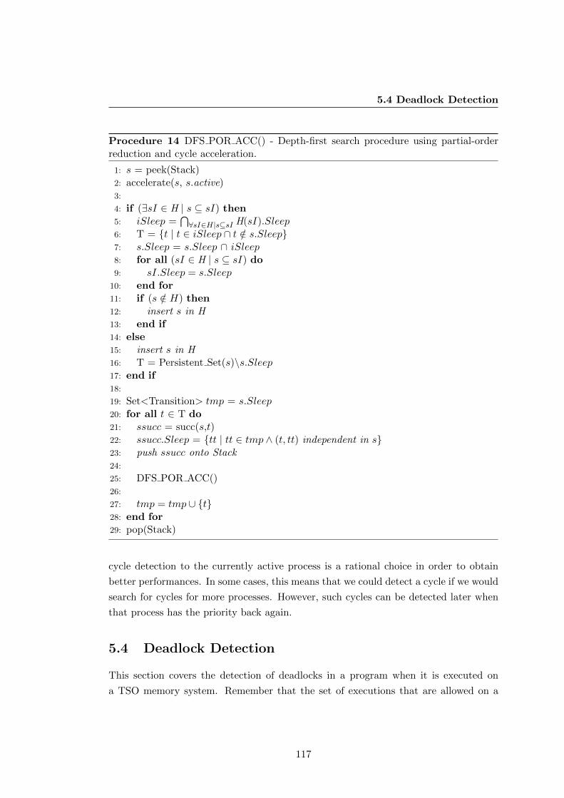
5.4 Deadlock Detection
Procedure 14 DFS POR ACC() - Depth-first search procedure using partial-orderreduction and cycle acceleration.
1: s = peek(Stack)2: accelerate(s, s.active)3:
4: if (∃sI ∈ H | s ⊆ sI) then5: iSleep =
⋂∀sI∈H|s⊆sI H(sI).Sleep
6: T = t | t ∈ iSleep ∩ t /∈ s.Sleep7: s.Sleep = s.Sleep ∩ iSleep8: for all (sI ∈ H | s ⊆ sI) do9: sI.Sleep = s.Sleep
10: end for11: if (s /∈ H) then12: insert s in H13: end if14: else15: insert s in H16: T = Persistent Set(s)\s.Sleep17: end if18:
19: Set<Transition> tmp = s.Sleep20: for all t ∈ T do21: ssucc = succ(s,t)22: ssucc.Sleep = tt | tt ∈ tmp ∧ (t, tt) independent in s23: push ssucc onto Stack24:
25: DFS POR ACC()26:
27: tmp = tmp ∪ t28: end for29: pop(Stack)
cycle detection to the currently active process is a rational choice in order to obtain
better performances. In some cases, this means that we could detect a cycle if we would
search for cycles for more processes. However, such cycles can be detected later when
that process has the priority back again.
5.4 Deadlock Detection
This section covers the detection of deadlocks in a program when it is executed on
a TSO memory system. Remember that the set of executions that are allowed on a
117
5. TOTAL STORE ORDER
TSO machine can contain more executions than the set of executions allowed on a SC
machine. Thus, even when there are no deadlocks in a program when executed under
SC, there might be a deadlock when the program is executed under TSO semantics. It
is thus important to be able to check the absence of deadlocks in this setting, which we
can do when relinquishing termination of the exploration of the state space.
Note that the problem addressed in this section is equivalent to the problem of
checking safety properties that is addressed in the next section. Indeed, any safety
property verification problem can be reduced to a deadlock detection problem, and any
deadlock detection problem can be expressed as a safety property verification problem.
The reason why we differentiate both cases is that computing persistent-sets can be
optimized for each of these settings. Safety property verification can be reduced to
deadlock detection as follows. A global state sd with no outgoing transition is added
to the system. Once a global state violating the safety property is reached, the system
can move to sd, and the deadlock is reached. Deadlock detection can be reduced to
safety property verification as follows. A deadlock is a global state with no outgoing
transitions. Thus, one only needs to generate the set of global states of all possible
combinations of control locations of the processes and a memory domain for which none
of the transitions of the processes can be executed in the corresponding state. Once
this set is computed, we can perform the safety property verification while looking if
one of the states in the generated set is reachable.
The general definition of a deadlock is the following, stating that from a given state,
no more state is possible to be reached. Note that if the program consists of only finite
executions, the last state of each execution consists in a deadlock but which is not
considered as a problematic deadlock because each execution will eventually reach such
an “end”-state. For systems that are intended to run continuously without halting, a
reachable state in which the program is blocked forever is a serious problem.
Definition 5.44. A state s in the state space is a deadlock if there is no enabled
outgoing transition from s.
Combining partial-order reduction with cycle acceleration has been shown to be
safe in the sense that if there exists a deadlock in the system, this deadlock will also
be present in the state space computed by our algorithm, see Theorem 5.43.
Another important question remains: how can deadlocks be detected when consid-
ering the fact that buffers may contain unbounded buffer contents which could make
the system continuously executing commit operations without being blocked, but where
118
5.5 Safety Property Verification
none of the processes of P can ever move on in its control graph. For this, we can adapt
the definition of a deadlock to TSO-deadlocks, and we get Definition 5.45.
Definition 5.45. A state s in the state space is a TSO-deadlock if there is no enabled
outgoing transition from s in which a process p ∈ P is active and if all buffers accept
the empty word, i.e. ∀p ∈ P, ε ∈ L(Ap).
In a TSO-deadlock state according to Definition 5.45, all buffer automata must
accept the empty word (these buffer automata may also accept other words). Such
a state contains thus a state satisfying the deadlock definition given above with no
outgoing transition possible to execute. If such a state is reached, the system is not
deadlock-free.
In order to detect deadlocks during the exploration of the state space by using the
depth-first search given in Procedure 14, we only need to watch out for states in which
all the buffers contain the empty word and which does not allow any other transitions
of p ∈ P to be executed (except for “end”-states of a program).
5.5 Safety Property Verification
In this section, we address the problem of verifying a safety property. Safety properties
are very commonly used to describe that some behaviors must never happen during
any execution of the system. Especially safety-critical systems are often encased by
safety properties. Definition 5.46 gives the definition of a safety property.
Definition 5.46. A safety property associated to a program expresses that something
“bad” must never happen in all executions of the program.
Such a “bad” behavior can be expressed as a global state of the system that violates
the safety property. In the context of mutual exclusion algorithms, the associated safety
property expresses that at most one process can enter into the critical section at a time.
This can be transformed into the problem of checking whether it is possible to reach a
global state in which two processes are in the critical section.
When using partial-order reduction to limit the size of the state space in the context
of safety property verification, the basic procedure of computing persistent-sets is not
sufficient. This is due to the fact that a partial-order search might “ignore” a process
and leave it totally inactive at some point (which is allowed when only verifying the
absence of deadlocks), which is known as the “ignoring problem” described in [31,
119
5. TOTAL STORE ORDER
71]. This problem can be handled by using a proviso condition as suggested in these
references. A proviso condition ensures that a persistent-set contains at least one
transition leading to a state that is not already on the current search path and that is not
contained in the sleep-set of the state which would avoid to execute this transition. In
other words, the proviso condition ensures that at least one transition will be executed
leading to a “new” state which is not already in the current search path. If such a
persistent-set does not exist, the set of transitions to be returned in this state by the
persistent-set computation is the set of enabled transitions in this state. Definition 5.47
gives the conditions a persistent must satisfy in order to satisfy the proviso condition
(taken from [31]).
Definition 5.47. Each time a call to the function persistent-set is performed during
the exploration, the persistent-set in s that is returned by the function has to satisfy the
following requirement:
1. either ∃t ∈ persistent-set(s) : t /∈ s.Sleep and s′ /∈ Stack, where s′ is the successor
of s by t, and s.Sleep is the sleep-set associated with s when the call is performed;
2. or persistent-set(s) = enabled(s).
However, computing persistent-sets by satisfying the proviso condition only guar-
antees the reachability of local states of the different processes, some global states
potentially being left unexplored. Thus, to force the detection of global error states
(those states violating a safety property), we consider as dependent in the context of
persistent-set computation those transitions that make a process leaving its control
location if this control location is part of a global error state. Such a global state is
labeled partial error state, in which at least one process is in a control location being
part of global error states.
Then, the procedure to compute a persistent-set in Procedure 14 satisfying the
proviso condition, and thus combining the persistent-set computation of Algorithm 12
and the proviso conditions of Definition 5.47, is the following. One searches for a process
whose only possible transitions (enabled or disabled) execute store or local operations
and satisfy the proviso condition, i.e., contains at least one transition leading to a state
that is not on the current search stack. If furthermore the control location of this
process in the current global state is not part of a global error state, the persistent-set
is taken to be the set of enabled transitions of this process. If such a process cannot
be found, the persistent-set is taken to be the whole set of enabled transitions of the
processes in P.
120
5.5 Safety Property Verification
Finally, we need to show that computing persistent-sets that satisfy a proviso con-
dition as well as taking into account partial error states as described above will not
be in conflict with the symbolic representation of our symbolic sets of states. Note
that the sleep-set computation is not affected by safety properties, and do not need
modification.
Theorem 5.48. Computing the state space by combining cycle acceleration with per-
sistent-sets that satisfy the proviso condition and that are sensitive to global error states
does not affect the reachability of global error states.
Proof. It is clear that the awareness of the partial error states cannot be in conflict with
the symbolic sets of states, because such partial error states do not take into account
the buffer contents.
Next, we deal with the proviso condition. Recall that the proviso condition is used
to ensure that, in each state, at least one transition in the persistent-set will lead to a
state which is not already on the current search-path.
When a state represents a single (or explicit) state, all previously established results
still hold. Otherwise, the reasoning is the following. Let s be a state in which a set
SEQ of mixable sequences has been accelerated. Executing again a sequence in SEQ
from s will lead to a state s′ in which this sequence is accelerated again, and s′ will
be identical to s after this acceleration. The transition that leads to s′ will not satisfy
the proviso condition, because s is already in the current search path (for this, we
perform cycle acceleration already during the computation of the persistent-set when
a successor state of the current state is considered). This holds for all the sequences
in SEQ. We will thus not constantly execute the transitions of the sequences in SEQ,
because soon or later in a state s′′, none of these will satisfy the proviso condition, and
the persistent-set in s′′ will contain either at least one transition that leads to a state
not belonging to the current search path, or all enabled transitions in that state. By
doing so, we ensure that we will not constantly ignore other behaviors than those where
a single process only stays in its mixable sequences, and we exactly meet the proviso
condition.
Finally, we can conclude that if there is a state violating a safety property, we
will not miss this state for the reason of accelerating cycles, and our approach safely
combines cycle acceleration and the persistent-set that satisfies a proviso condition and
that is aware of global error states.
121
5. TOTAL STORE ORDER
5.6 Moving from SC to TSO
We now turn to the problem of preserving the correctness of a program when it is
moved from an SC to a x86-TSO memory system. By correctness, we mean preserving
state (un)reachability properties (absence of deadlocks and satisfied safety properties).
An obvious way to make sure a program can safely be moved from SC to x86-TSO is
to force writes to be immediately committed to main memory by inserting an mfence
operation after each store, thus precluding any process from moving with a nonempty
buffer content. The obvious drawback of doing so is that any performance advantage
linked to the use of store buffering in the implementation is lost.
However, this is more than necessary to guarantee that the executions that are
allowed under TSO semantics are also possible under SC semantics. Recall that the
difference between the axiomatic definitions of SC and TSO is the absence of the fol-
lowing store-load constraint in TSO, where l denotes any load, s denotes any store and
where <p and <m are respectively the program order and the memory order of memory
accessing operations:
∀l, s : s <p l⇒ s <m l (5.3)
Thus, stores can be postponed in memory order after later loads, leading to exe-
cutions that are not possible in SC. To avoid this, it is sufficient to make sure that
no process can execute a load after a store without going through an mfence. Indeed,
even if successive stores might be buffered, they will be committed to main memory
in program order before any later load and hence the constraint in Equation 5.3 will
be satisfied by the memory order, just as in SC. The memory order then becomes an
interleaving of the program orders and the execution semantics thus match SC. We
formalize this in the following lemma.
Lemma 5.49. Given an x86-TSO execution, if in the program order of each process,
an mfence is executed between each load and any preceding store, the memory order
satisfies all the SC constraints.
Proof. The semantics of mfence operations can be formalized by introducing these
operations in the memory order with the following constraints, s, l and m representing
store, load and mfence operations respectively:
1. ∀s,m : s <p m⇒ s <m m
2. ∀s,m : m <p s⇒ m <m s
122
5.6 Moving from SC to TSO
3. ∀l,m : l <p m⇒ l <m m
4. ∀l,m : m <p l⇒ m <m l
In the conditions of the lemma, we have that if s <p l, there is an mfence m such
that s <p m and m <p l. And thus we have that s <m l, using the semantics of
mfences.
The memory order thus satisfies all constraints of an SC order.
Remark 5.50. Using Lemma 5.49, one can deduce that for any algorithm that writes
to memory exclusively with processor instructions including implicitly a memory bar-
rier1 (such as the atomic operations CAS (compare-and-swap) or TAS (test-and-set)),
moving these algorithms from SC to TSO will preserve their correctness.
The Micheal-Scott non-blocking queue [57] is such an algorithm in which all memory
write operations to shared memory are implemented by the atomic CAS operation, and
thus will run correctly under TSO semantics. This observation is consistent with the
results in [40].
We now have a sufficient condition for guaranteeing correctness while moving from
SC to x86-TSO. The condition is expressed on executions, but can easily be mapped
to a condition on a program: in the control graph of the program, an mfence must be
inserted on all paths leading from a store to a load. This is sufficient, but can insert
many unnecessary mfence instructions. The next section will propose an approach that
aims at only inserting those mfence instructions that are needed to correct errors that
have actually appeared when moving the program to TSO.
5.6.1 Error Correction: Iterative Memory Fence Insertion
This section proposes a way how to modify a program after which the program can
safely be moved from SC to TSO while guaranteeing correctness (with respect to state-
reachability problems). For this, we only consider programs that satisfy the correctness
criterion when executed under SC semantics. The outline of this iterative mfence
insertion procedure is given in Algorithm 15. In order to find quickly states violating
the current property, we can influence the scheduling of the operations that are to be
executed in a given state. In particular, we will prevent as long as possible a process
to proceed if its control location is part of a global state that should not be reachable.
1A memory barrier is a memory fence
123
5. TOTAL STORE ORDER
Algorithm 15 Outline of the iterative mfence insertion algorithm.
Run the state-space exploration algorithm using cycle detection, cycle accelera-tion and partial-order reduction until either reaching a state violating a correct-ness criterion or having computed the entire state space without reaching an errorstate;
If an error state is reached, search for a place where to insert an mfence operationin order to make the undesirable state unreachable and the mfence operation isinserted into the program;
Repeat this procedure until no further bad state can be reached.
The central algorithm is modified in order to manage the iterative mfence inser-
tion until no more error states can be reached, Algorithm 16. Additionally, the DFS-
procedure in 14 is modified such that for each state we visit, we additionally check if it
violates the correctness criterion. If it doesn’t, the exploration continues. If the state
violates the criterion, we need to modify the program by inserting an mfence opera-
tion. After this modification, we need to notify the iterative mfence insertion algorithm
that the program has been modified and that the exploration must be restarted with
the modified program. This notification can be achieved by making the DFS explo-
ration function to return the Boolean value false if an error state was reached, while
it returns true if the exploration terminates without detecting any error state. The
modified DFS-procedure is given in Procedure 17.
Algorithm 16 Iterative mfence insertion algorithm.
1: repeat2: init(Stack) /* Stack representing the current search path */3: init(H) /* Table of visited states */4: s0 = initial state5: push s0 onto Stack /* put initial state on stack */6: until (DFS POR ACC MFENCE INSERTION())
We need to detail how a place for an mfence operation to avoid reaching the current
error state is computed when the function insertMfence() in Procedure 17 is called.
Since we start with a program that is considered to be correct under SC, an undesirable
state only can be reached because of the weaker TSO semantics. Comparing TSO to
SC, and using the same line of reasoning as the one leading to Lemma 5.49, this
can only happen if a load is performed by a process when the corresponding buffer
124
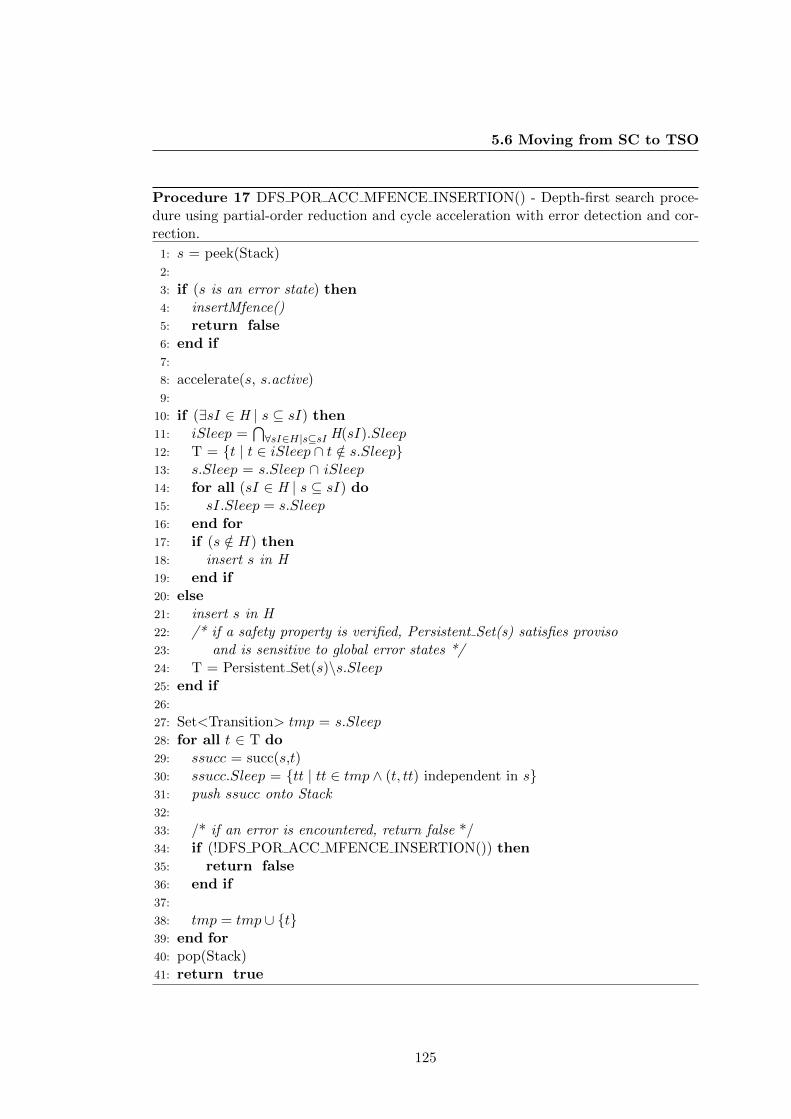
5.6 Moving from SC to TSO
Procedure 17 DFS POR ACC MFENCE INSERTION() - Depth-first search proce-dure using partial-order reduction and cycle acceleration with error detection and cor-rection.
1: s = peek(Stack)2:
3: if (s is an error state) then4: insertMfence()5: return false6: end if7:
8: accelerate(s, s.active)9:
10: if (∃sI ∈ H | s ⊆ sI) then11: iSleep =
⋂∀sI∈H|s⊆sI H(sI).Sleep
12: T = t | t ∈ iSleep ∩ t /∈ s.Sleep13: s.Sleep = s.Sleep ∩ iSleep14: for all (sI ∈ H | s ⊆ sI) do15: sI.Sleep = s.Sleep16: end for17: if (s /∈ H) then18: insert s in H19: end if20: else21: insert s in H22: /* if a safety property is verified, Persistent Set(s) satisfies proviso23: and is sensitive to global error states */24: T = Persistent Set(s)\s.Sleep25: end if26:
27: Set<Transition> tmp = s.Sleep28: for all t ∈ T do29: ssucc = succ(s,t)30: ssucc.Sleep = tt | tt ∈ tmp ∧ (t, tt) independent in s31: push ssucc onto Stack32:
33: /* if an error is encountered, return false */34: if (!DFS POR ACC MFENCE INSERTION()) then35: return false36: end if37:
38: tmp = tmp ∪ t39: end for40: pop(Stack)41: return true
125
5. TOTAL STORE ORDER
is nonempty. Thus, the procedure inserting an mfence starts from the detected error
state and searches backwards through the current search path for such a situation. We
could directly insert an mfence just before the offending load in the code of the process
executing it, but this would be suboptimal if the previous instruction was a load and
not a store, given that only store to load transitions are problematic. The backwards
search is thus continued until a store executed by the same process as the offending
load is found. When this store operation is detected, we insert an mfence operation
right after it in the control graph of the process.
Note that we just insert one mfence at each run of the verification procedure. This
means that the procedure will usually be run repeatedly, but since the number of pos-
sible mfence operations is bounded by the size of the program, the iterative process will
always terminate when supposing that the state space can be constructed. Moreover,
as we only insert necessary mfence operations, the number of mfences inserted is in this
sense optimal, but the optimal is clearly local: there is no guarantee that we always
reach a globally minimal number of mfences inserted, and it might happen that after
the algorithm has iteratively inserted a number of mfences, an mfence that was inserted
becomes unnecessary due to mfences inserted later. However, one can, after inserting
enough mfences to preserve the correctness of the program, reiterate over the inserted
mfences by removing an mfence and checking if an error state can be reached. If so, the
mfence is needed, and if not, we can safely remove it. After repeating this procedure
until no more mfences can be removed, we obtain a set of mfences called “maximal per-
missive”, meaning that each mfence is needed to ensure the correctness criterion. This
does not however imply that the set of inserted mfences is globally minimal since the
set obtained is dependent of the order in which the mfences are inserted and removed.
A more elaborated approach computing all maximal permissive sets of mfences was
proposed in [1] and [2]. The computation of the maximal permissive sets of mfences
works by building sets of mfences using traces leading to error states generated by their
reachability algorithm. As our approach also finds traces leading to error states, their
computation of all globally maximal permissive sets of mfences is compatible with our
state-space exploration approach.
126
Chapter 6
Partial Store Order
This chapter extends the verification approach presented in the previous chapter to
the memory model called Partial Store Order (PSO), see Section 3.3, again without
restricting in any way the size of the store buffers. More specifically, the techniques
presented allow the verification of safety properties of programs analyzed under PSO
with unbounded memory buffers. Additionally, we propose an approach that can mod-
ify a program in order to preserve a safety property, which is satisfied by the program
under SC or TSO, but violated when the program is moved onto a PSO system. For
the latter, the basic PSO memory model is not sufficient, and the extended-PSO model,
see Section 3.4.2, which includes two fence operations, is clearly needed.
As for TSO, we will first in Section 6.1 give precise semantics of the operations
of the system under extended-PSO semantics. The most important of them already
were given in [47], while others were omitted in that work. Section 6.2 covers the cycle
acceleration in the case of PSO, which will turn out to be very easy after providing
the acceleration technique under TSO, and which also has been introduced in [47]. In
Section 6.3, the partial-order reduction technique is adapted for its use under PSO.
Section 6.4 covers the verification of the absence of deadlocks as well as the verification
of safety properties. Finally, Section 6.5 gives a criterion in order to ensure that all
executions allowed under PSO correspond to executions under either TSO or SC, which
can be achieved by adding memory fences into the program. Moreover, a procedure is
proposed that ensures to preserve a given property associated to a program when this
program is moved onto a PSO memory system, which was also presented in [47].
127
6. PARTIAL STORE ORDER
6.1 Buffer Operations
In this section, we give the precise semantics of all memory operations. For each
operation, we specify whether the operation is buffer-preserving or buffer-modifying,
which is needed when analyzing independence of transitions in Section 6.3. Most of the
memory operations are very similar to their counterpart under TSO, and we can safely
omit any illustration of the operations.
Recall that a global state s is composed of a control location for each process,
a different buffer automaton for each variable associated to each process, a memory
content for each memory location and a value for the global lock that can either be a
process p ∈ P or ⊥. In the initial state, all buffers are set to the empty buffer. The
control location for each process p ∈ P in a state s can be accessed by the function
cp(s), the memory content of variable m ∈ M can be accessed by m(s), each buffer
b(p,m) ∈ B can be accessed by b(p,m)(s) or by A(p,m)(s), and the value of the lock can be
accessed by Lock(s). The current global state is denoted s, and the successor state after
executing t = `op→ `′ from s is denoted s′, where op is the operation being executed. A
second notation for the computation of the successor state of s by executing t to reach
s′ is to write s′ = succ(s, t), where succ is the function returning the successor state of
s when executing t from s. Also recall that the buffer contents may be composed by
elements of (1) (m, v), where (m, v) ∈M×D, and (2) special symbols bt representing
an sfence(p)-transition t.
6.1.1 Store Operation
The first operations for which we need to give the semantics is the store operation. It
is the following:
store(p, m, v)
Let A(p,m) be the buffer automaton associated to p for m in s. Then, the result of
the store operation is an automaton A′(p,m) associated to p for m in the successor
state s′ such that
L(A′(p,m)) = L(A(p,m)) · (m, v),
where L(A) denotes the accepted language of the automaton A. One thus simply
concatenates that new stored value to the memory to all words accepted by the
automaton.
128
6.1 Buffer Operations
A store operation is always buffer-preserving, since no content of the buffer present in
state s is disallowed by the operation.
6.1.2 Load check Operation
Again, as for TSO, the load check operation is more delicate, since a load check opera-
tion may succeed on some buffer contents but can fail on others. To ensure consistency,
once a load check operation has succeeded for some value, the set of buffer contents
must be restricted to those on which the load check operation is actually successful for
that value. This could include those buffer contents which do not contain any value for
the given variable if the requested value is found in the shared memory for this memory
location. However, the very first step is to ensure that the global lock is not taken by
another process in order to allow the load check operation to be executed. The exact
semantics of the load check operation is the following:
load check(p, m, v)
If the global lock is held by another process, i.e., Lock(s) = p′, then the operation
cannot be executed.
Otherwise, we proceed as follows. For a load check operation to succeed, the
tested value must be found either in the corresponding store buffer or in main
memory. Precisely, a load check operation succeeds when at least one of the
following two conditions is satisfied:
1. The language
L1 = L(A(p,m)) ∩ ((Σm)∗ · (m, v) · (Σb)∗)
is nonempty, where Σm ⊆ Σ denotes those symbols possible in A(p,m), A(p,m)
denotes the buffer automaton of p for m in s, and where Σb ∈ Σ denotes
the sfence-symbols.
2. The language
L2 = L(A(p,m)) ∩ (Σb)∗
is nonempty and m(s) = v.
The first condition ensures that words are only retained in the set of accepted
buffer contents if, at one point in a retained word, there is a symbol representing
(m, v), where that (m, v) either is the last element in the buffer content or followed
129
6. PARTIAL STORE ORDER
by only sfence symbols. The second condition ensures that, in case where the
value of m in the shared memory (m(s)) is equal to v, only those words are
retained which do not contain any symbols representing store operations.
The load check operation then leads to a state with a modified buffer automaton
A′(p,m) for m of p in the successor state such that
L(A′(p,m)) = L1 ∪ L2
if m(s) = v and
L(A′(p,m)) = L1
otherwise. Of course, if L1 ∪ L2 = ∅, the load check operation is simply not
possible.
As already said, once a load check operation has succeeded for some value v, we
ensured consistency by potentially removing some of the buffer contents from
the buffer on which the load check does not succeed. But as we are now dealing
with PSO, special care should be applied if bt symbols are present in the buffer
contents. Indeed, if a bt symbol is removed when modifying a buffer to take into
account that the load check has succeeded, the synchronization required by that
sfence symbol will no longer be possible, thus potentially introducing a spurious
deadlock because other buffers maybe need the removed sfence symbol to stay
in the current buffer in order to allow the synchronized commit of that sfence
symbol. If this occurs, there are two possibilities: (1) the buffers for the other
variables of the process are also modified in order to remove the now spurious
bt symbols, or (2) if this is not possible because the spurious bt symbol are
part of each buffer content of another variable, the current load check operation
cannot be executed because it would violate the introduced synchronization of
the sfences.
This is achieved as follows (but is only needed in the case that the load check
operation modified the buffer contents).
We first need to figure out which bt symbols are still available in the buffer
contents of p for m after executing the load check, and in which combinations
they can appear. For this, we compute Ab as follows. We initialize Ab = A′(p,m).
Let δ1 ⊆ δAb be the set of transitions in Ab reading a symbol from Σ \ Σb.
These transitions are modified such that they now read the empty word. Note
that in practice, we only work with deterministic automata. However, for the
130
6.1 Buffer Operations
construction of Ab to be more easy to understand, we can use non-deterministic
automata. We can do so without loss of generality as each non-deterministic
automata can be determinized. Then, we add a transition from each state in Ab
to itself that reads a symbol in Σ \ Σb. Finally, Ab accepts all buffer contents
satisfying the same bt combinations than A′(p,m) does accept.
Then, we need to restrict all buffer automata associated to p different from A′(p,m)
to only accept those buffer contents that are compatible with A′(p,m) in terms of
the accepted bt combinations. So, we compute A′(p,m′) = A(p,m′) ∩ Ab for all
m′ ∈M \ m, where A′(p,m) is the buffer automaton of p for m in the successor
state of s after executing the load check operation. If however at least one of these
intersection-computations returns an empty set of buffer contents, we know that
by executing the current load check operation, the introduced synchronization is
violated and the load check operation cannot be executed.
A load check operation is buffer-preserving if, for the accessed location, there is only
one possible value to be loaded from the buffer and the shared memory. In this case,
the load check operation is either possible to execute while not modifying at all the
buffer automata of the active process, or simply not possible to execute because the
associated check cannot not be passed. Otherwise, the operation is buffer-modifying,
because some contents will be removed from the sets of buffer contents, in order to be
consistent with the executed load check operation and the sfence-symbol handling.
6.1.3 Load Operation
The load operation is (as under TSO) partially identical with the load check operation,
but starts differently. After verifying that the global lock is not held by another pro-
cess, all possible values to be loaded from the buffer or from the shared memory are
computed. Note that loading from the shared memory is only possible when the buffer
content does not include any store operations (note that it can include some sfence-
symbols). Once all these possible values are computed, there will be one successor state
per possible load value, while the resulting buffer is computed in the same way as the
load check operation does, the loaded value being the one checked for and assigned to
the local register. The exact semantics of the load operation is the following:
load(p, m, r)
If the global lock is held by another process, i.e. Lock(s) = p′, then the operation
cannot be executed.
131
6. PARTIAL STORE ORDER
Otherwise, we proceed as follows. First, we need to compute the possible values
to be loaded. For this, we construct a set of values Ω such that each ω ∈ Ω can
be either loaded from the buffer for variable m of process p or from the shared
memory.
We start with adding all possible values to be loaded from the buffer A(p,m)(s).
For this, we need the last stored values of all buffer contents in L(A(p,m)). We
find these by looking for the value of the first buffer element different from an
sfence symbol in the prefixes of the inverted buffer language. Let Σb ⊆ Σ be the
buffer elements corresponding to sfence-symbols. The resulting language is L1,
and is then computed as follows.
L1 =[prefix(L(A(p,m))
R) ∩ ((Σb)∗ · (m, v) | v ∈ D)]R.
All words in L1 will then start with elements of (m, v) | v ∈ D, followed by
words in (Σb)∗. Then, if L1 is nonempty, the first elements of its words, i.e., the
language of singletons first(L1), contains the pairs (m,α) such that the value α
can be loaded from the buffer, and we add all these α to Ω.
Second, we need to check if there are buffer contents allowing the value to be
loaded from the shared memory, i.e., if there are buffer contents not containing
any store operation but at most a series of sfence symbols. For this to check, we
compute L2:
L2 = L(A(p,m)) ∩ (Σb)∗.
Then, if L2 is non empty, we add m(s) to Ω.
Once Ω has been computed, we compute, for each ω ∈ Ω, an automaton A′(p,m)(ω)
that would be obtained for the operation load check(p,m, ω) on A(p,m), represent-
ing the buffer automaton of p for m in the successor state when the value ω was
loaded. Finally, we save the loaded value, ω, to the local register r.
For the load operation, we must again take special care about the sfence symbols
that might be in the buffer contents accepted by the current buffer automaton.
Then, the subsequent call to the load check operation might remove some sfence
symbols from the buffer contents, hence we need either to modify again the buffer
contents of the other buffers associated to p if possible (which is done exactly in
the same way as we did for the load check operation), or, if this is not possible,
not allow the execution of the current load operation.
132
6.1 Buffer Operations
A load operation is buffer-preserving if there is only one possible value to be loaded
from the buffer and the shared memory. Otherwise, it is buffer-modifying.
6.1.4 Commit Operation
When the global lock is held by some process, only this process is allowed to execute any
commit operation. If the buffer has several possible contents, the commit operation can
yield a different result for each and we need to consider them all. The exact semantics
of the commit operation is the following.
commit(p,m)
If the global lock is held by another process, i.e., Lock(s) = p′, then the operation
cannot be executed.
Otherwise, we proceed as follows. We first extract the set Ω of store/sfence
operations from the buffer for m of p such that the elements of Ω are these
store/sfence operations that can be removed from the buffer, but where only
store operations will be committed to the shared memory. We have that Ω =
αi | αi ∈ first(L(A(p,m)(s))), where each αi represents either a pair (m, v) or a
bt-symbol.
Then, for each possible element α ∈ Ω \ Σb, we need to compute an automaton
according to the currently committed store operation leading to s′. We have
L(A′(p,m)((α))) = suffix1(L(A(p,m)) ∩ ((α) · Σ∗)),
where suffix1(L) denotes the language obtained by removing the first symbol of
the words of L. After updating the buffer contents with the currently committed
store operation, we again need to take special care of the potentially removed
sfence symbols, and either update the other buffers of p accordingly or to not at
all execute the current commit operation.
For all α ∈ Ω∩Σb representing sfence transitions, the commit operation is either
blocked (in case that this sfence symbol is not possible to be removed from each
buffer content of p in s) or removes in a synchronized way the sfence symbol from
each buffer content of p in s.
The condition of commit operation to be buffer-preserving for A(p,m) is the following. If
the function first(A(p,m)(s)) only returns one possible symbol α and ε /∈ A(p,m) and the
execution of the commit does not require other buffers of the process to be modified due
133
6. PARTIAL STORE ORDER
to sfence-symbol handling, then the commit operation is buffer-preserving. Otherwise,
the commit is buffer-modifying.
6.1.5 Mfence Operation
The mfence operation is a simpler operation. It is only possible if the buffer contents
of all the buffers of the executing process accept, possibly among others, the empty
word. However, once the mfence operation is executed, the buffers are required to only
have the empty word as possible content. The semantics of the mfence operation is the
following.
mfence(p)
First, one needs to check if the all buffer automata of p accept the empty word
in s, i.e., if ∀m ∈ M, ε ∈ L(A(p,m)(s)). If this is the case, the mfence operation
is possible, and the resulting buffer automata of p in s′ only accept the empty
word, i.e., ∀m ∈M, L(A(p,m)(s′)) = ε. Otherwise, the mfence operation is not
possible.
If the buffer automata of process p all only accept the empty word, then the mfence
operation is buffer-preserving. If at least one buffer content may also contain other
words, the mfence operation is buffer-modifying.
6.1.6 Sfence Operation
The sfence operation is used to disable store-store relaxations, and adds the sfence
symbol corresponding to the current transition to each buffer content in all the buffers
associated to the executing process. The semantics is the following.
sfence(p)
Let A(p,m) be the buffer automaton associated to p for m in s. Then, the result of
the sfence operation is an automaton A′(p,m) associated to p for m in the successor
state s′ such that
L(A′(p,m)) = L(A(p,m)) · bt,
where L(A) denotes the accepted language of the automaton A and where t is
the transition executing the sfence operation. One thus simply concatenates that
sfence symbol to all words in the language of the automaton.
134
6.1 Buffer Operations
An sfence operation is always buffer-preserving, since no content of the buffer present
in state s is disallowed by the operation.
6.1.7 Lock Operation
The lock operation only is possible to execute if the global lock has not already been
taken by another process. The semantics of the lock operation is the following.
lock(p)
If (Lock(s) = p or Lock(s) =⊥), then lock(p) is enabled and the execution results
in a global state s′ in which Lock(s′) = p;
otherwise, lock(p) cannot be executed.
The lock operation is always buffer-preserving, because no buffer is accessed.
6.1.8 Unlock Operation
The unlock operation can only be completed if the sequence of locked instructions
(and consequently also all previous operations) is entirely visible globally. The unlock
operation is thus only possible when the buffers of the executing process have the empty
word as possible content. If so, the result of the unlock operation is to release the lock
and the buffers are set to the empty buffer. If not, the unlock operation is not possible
and the lock is still held by the executing process. The semantics is the following.
unlock(p)
If (Lock(s) = p and ∀m ∈ M, ε ∈ L(A(p,m))), then Lock(s′) =⊥ and ∀m ∈M, L(A′(p,m)) = ε, where A(p,m) is the buffer for m of p in s and A′(p,m) is the
buffer in the successor state s′ of p for m;
otherwise, unlock(p) cannot be executed.
The unlock operation is buffer-preserving if all the buffers of process p only contain the
empty word. If at least one buffer of p contains other contents alongside the empty
word, the operation is buffer-modifying because the contents will be restricted in order
to only contain the empty word.
135
6. PARTIAL STORE ORDER
6.1.9 Local Operation
Local operations under PSO have exactly the same semantics than under TSO, and
need no further details.
Any local operation is always buffer-preserving.
6.1.10 Discussion on Operations
As in Section 5.1.9, one can make several statements about the operations and the
buffers. For example, each buffer will eventually be emptied and thus an operation
that is not possible to execute due to a non-empty buffer will become so in some
successor state of s because of the non-deterministic execution of commit operations
in every global state. Moreover, we again consider that the commit operations are
executed by the buffer-emptying process, called pb. This process only has one control
location, and its enabled transitions in a state s are the possible commit operations to
be executed on any buffer, while pb always stays in its single state. Every commit(p)
operation become thus an operation where process pb is the active one. This modeling
will make it easier to determine independence of transitions when considering partial-
order reduction (Section 6.3).
6.2 Cycles
This section focuses on the problem of the potential infinite size of the system due to
the introduction of the store buffers in order to model PSO. Recall that there is a set
of store buffers associated to each process under PSO instead of a single store buffer
under TSO. Thus, we need to handle a set of store buffers per process, one for each
variable. Additionally, we need to handle sfence operations. The state-space explo-
ration including the detection of cycles is done exactly as for TSO. What changes are
the operations applied to the buffer automata to accelerate the cycles: rather than op-
erating on a single buffer automaton for each cycle, the one corresponding to the active
process, we need to operate on multiple automata, one for each updated variable of the
active process. The obvious way is to filter from the cycle the operations corresponding
to each variable and only consider these when dealing with the corresponding buffer
automaton. This is straightforward to implement, but generates more buffer contents
that can actually occur: the link between the number of times write operations are
applied to different variables is lost! To make this clear, let us consider the following
136
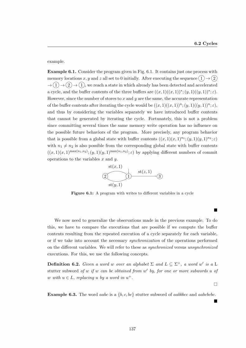
6.2 Cycles
example.
Example 6.1. Consider the program given in Fig. 6.1. It contains just one process with
memory locations x, y and z all set to 0 initially. After executing the sequence 1 → 2
→ 1 → 2 → 1 , we reach a state in which already has been detected and accelerated
a cycle, and the buffer contents of the three buffers are ((x, 1)((x, 1))∗; (y, 1)((y, 1))∗; ε).
However, since the number of stores to x and y are the same, the accurate representation
of the buffer contents after iterating the cycle would be ((x, 1)((x, 1))n; (y, 1)((y, 1))n; ε),
and thus by considering the variables separately we have introduced buffer contents
that cannot be generated by iterating the cycle. Fortunately, this is not a problem
since committing several times the same memory write operation has no influence on
the possible future behaviors of the program. More precisely, any program behavior
that is possible from a global state with buffer contents ((x, 1)(x, 1)n1 ; (y, 1)(y, 1)n2 ; ε)
with n1 6= n2 is also possible from the corresponding global state with buffer contents
((x, 1)(x, 1)max(n1,n2); (y, 1)(y, 1)max(n1,n2); ε) by applying different numbers of commit
operations to the variables x and y.
2 1 3
st(x, 1)
st(y, 1)
st(z, 1)
Figure 6.1: A program with writes to different variables in a cycle
We now need to generalize the observations made in the previous example. To do
this, we have to compare the executions that are possible if we compute the buffer
contents resulting from the repeated execution of a cycle separately for each variable,
or if we take into account the necessary synchronization of the operations performed
on the different variables. We will refer to these as synchronized versus unsynchronized
executions. For this, we use the following concepts.
Definition 6.2. Given a word w over an alphabet Σ and L ⊆ Σ+, a word w′ is a L
stutter subword of w if w can be obtained from w′ by, for one or more subwords u of
w with u ∈ L, replacing u by a word in u+.
Example 6.3. The word aabc is a b, c, bc stutter subword of aabbbcc and aabcbcbc.
137
6. PARTIAL STORE ORDER
Definition 6.4. A sequence of operations that does not modify the store buffer in a
way that affects the result of subsequent load operations is called load-preserving.
We can then formalize the fact that repeating load-preserving sequences of commit
operations have no real impact on an execution.
Lemma 6.5. Le σ be an execution of a concurrent system and let LE be the set of
load-preserving commit operation sequences appearing in σ. Then every LE stutter
subword σ′ of σ is also a valid execution of the system.
Proof. This is a direct consequence of the fact that load-preserving sequences of commit
operations are idempotent, i.e., applying them one or several times has no effect on the
rest of the execution.
From this Lemma, it is easy to establish the property we need.
Theorem 6.6. Computing the buffer automata of different variables independently only
leads to valid executions.
Proof. Indeed, the potentially incorrect executions that could be obtained by handling
the buffers for different variables independently are those in which the number of stores
to variables executed in the same cycle could be taken to be different. Notice that this
will only have an effect on the execution when these stores are committed to memory
and that committing the stores appearing on a cycle is load-preserving. Thus, such
an unsynchronized execution will always be a LE stutter subword of a synchronized
execution, where LE is the set of load-preserving commit sequences corresponding to
cycles, and hence will be valid. Indeed, since we allow unbounded repetition of cycles,
the synchronized execution can be taken to be the one in which the cycle is repeated a
number of times greater than the largest number of times a store to any of the variables
modified in the cycle is committed to memory.
This theorem establishes thus that we can safely ignore the fact that our PSO buffer
computation ignores synchronization issues between the store buffers of a given process,
and all algorithms proposed for TSO also apply for PSO by considering a set of store
buffers for each process instead of a single store buffer.
138
6.3 Partial-Order Reduction
6.3 Partial-Order Reduction
In this section, we give the details on how partial-order reduction is used under PSO.
For this, we need to give the independence relation, the persistent-set computation as
well as to precise how the sleep-sets are handled.
6.3.1 Independence Relation
The formal definition of independent transitions was given in Definition 4.1 in Sec-
tion 4.2.1 alongside with sufficient syntactic conditions for transitions to be indepen-
dent. The introduction of the buffer emptying process pb facilitates the study of inde-
pendent transitions.
6.3.1.1 Transitions of the Same Process
When considering transitions of the same process, we only need to consider pairs of
transitions executing commit operations. All other pairs of transitions of the same
process are considered to be dependent.
Remember Remark 5.16 in which a more compact way of describing transitions was
given.
First, we consider commit transitions that access buffers of different processes, both
accessing different memory locations, or accessing the same memory location but up-
dating the location with the same value, or even when at least one of the commits
removes an sfence symbol.
Lemma 6.7. Two commit transitions t1 and t2 accessing buffer automata of different
processes are independent if t1 and t2 update different memory locations, or if t1 and
t2 update the same memory location with the same value, or if at least one removes an
sfence symbol.
Proof. We prove this by the formal definition of independent transitions. Let c1 be
the commit operation executed in t1 and c2 be the one executed in t2. It is clear that
a commit operation accessing one buffer cannot enable of disable a commit operation
accessing another buffer of a different process, and thus the first condition is satisfied.
Let s be a state in which both are enabled. By the conditions of the lemma, both c1
and c2 update different memory locations or the same location with the same value
or even at least one removes an sfence symbol from its buffer having no effect on the
memory, and executing the sequence t1,t2 or t2,t1 from s leads to the same state in
139
6. PARTIAL STORE ORDER
which both buffers have executed their commits and where the memory is updated in
the same way, and the second condition is satisfied as well.
Next, we analyze the independence of two commit transitions accessing different
buffers of the same process.
Lemma 6.8. Two commit operations t1 and t2 accessing different buffer automata
of the same process (by operations c1 and c2 respectively) are independent if c1 and
c2 are both either buffer-preserving or not restricting the buffer contents of the buffer
corresponding to the other commit (due to sfence-symbol handling).
Proof. Again, this can easily be proven by exploiting the formal definition of inde-
pendent transitions. Let c1 and c2 be the commit operations executed in t1 and t2
respectively. Let b1 and b2 be the buffers accessed in t1 and t2. It is clear that, by
the conditions of the lemma, a commit operation accessing one buffer cannot enable or
disable a commit operation accessing another buffer of the same process, and thus the
first condition is satisfied. Let s be a state in which both are enabled. The conditions
of the lemma specify that both c1 and c2 will (1) not restrict the buffer contents of the
buffer automaton corresponding to the other commit and (2) update different memory
locations, and thus both executions t1, t2 and t2, t1 from s will lead to the same state,
and t1 and t2 are thus independent.
The lemma corresponding to the cases with two independent commits accessing the
same buffer automaton is identical to the lemma given for TSO, Lemma 5.18.
6.3.1.2 Transitions of Different Processes
When studying independence of transitions where different processes are active, one
has to differentiate between pairs of transitions of p1 and p2 where p1, p2 ∈ P, and
pairs of transitions of p and pb where p ∈ P and where pb being the buffer emptying
process. We already developed similar proofs in the case of TSO, and we do not need
to prove all these independence statements again. Though, we need to slightly adapt
the definition of the set Proc-Local of operations which only have an effect either on
the executing process or on a buffer of the executing process.
Definition 6.9. The set Proc-Local contains operations of the type store, local, mfence
and sfence.
140
6.3 Partial-Order Reduction
After this, Lemmas 5.20-5.28 also hold in the case of PSO. The only additional
information that needs to be given is that Lemmas 5.25-5.28 handling the pairings
(store,commit) also apply for the pairings (sfence,commit), as executing an sfence is
basically executing a store but where the symbol represents an sfence transition and
not a store transition.
Then, we only need to cover explicitly the following pairs, which are very similar
to those under TSO, but differ only by the fact that we need to handle a set of buffers
for each process in the current PSO semantics instead of a singe buffer under TSO. For
this reason, we omit the proofs.
First, we need to handle the pairs of a load and a commit.
Lemma 6.10. A load transition t1 on buffer A(p,m) is independent from a commit
transition t2 on the same buffer if both t1 and t2 are buffer-preserving.
Proof. Similar to the proof of Lemma 5.29.
Lemma 6.11. A load transition t1 on buffer A(p,m) is independent from a commit
transition t2 on a buffer of a different process if t1 does-not-see the effect of t2.
Proof. Similar to the proof of Lemma 5.31.
Then, we cover the pairings of mfence and commit operations.
Lemma 6.12. In a state s, an mfence transition t1 of process p is independent from a
commit transition t2 accessing a buffer of p if that buffer of p only contains the empty
word.
Proof. Similar to the proof of Lemma 5.32.
Lemma 6.13. In a state s, an mfence transition t2 of process p is independent from
a commit transition t2 accessing a buffer of a different process.
Proof. Similar to the proof of Lemma 5.33.
Then, we consider the pairs of an unlock and a commit operation.
141
6. PARTIAL STORE ORDER
Lemma 6.14. In a state s, an unlock transition t1 of process p is independent from a
commit transition t2 accessing a buffer of p when that buffer only contains the empty
word.
Proof. Identical to proof of Lemma 5.34.
Again, we did not consider the load check operations explicitly, but implicitly, as it
was already described in Remark 5.35.
6.3.2 Persistent-Sets and Sleep-Sets
The computations of the persistent-sets under PSO is done exactly in the same way
as they are computed under TSO. Again, we compute the persistent-sets by satisfying
the conditions of a stubborn-set, which is the case when a process only has local or
store operations to execute in a given state. The algorithm is the same as for TSO, see
Algorithm 12, which can be proven to always compute persistent-sets under PSO as
well. As the proof is identical to the one in case of TSO (see Theorem 5.37), we omit
it.
Sleep-sets also are computed and updated in the same way as they were under TSO,
while the only difference are the modified independence relation under PSO and the
inclusion-relation of global states under PSO, see Definition 6.15. We can thus also
omit the procedure which updates the sleep-set of a state during a re-exploration of
the state, but which can be found in Procedure 13.
Definition 6.15. A state s1 is included in a state s2 with respect to PSO if the following
conditions are satisfied:
∀p ∈ P : cp(s1) = cp(s2)
∀m ∈M : m(s1) = m(s2)
Lock(s1) = Lock(s2)
∀p ∈ P, ∀m ∈M : L(A(p,m)(s1)) ⊆ L(A(p,)(s2))
Combining partial-order reduction and cycle acceleration is also safe under PSO,
as it was under TSO. Lemma 5.41 also holds, stating that the sleep-set associated to a
symbolic state is equal or smaller to those that would be associated to each of states
represented by the symbolic states when these states are reached without acceleration.
142
6.4 Deadlock Detection and Safety Property Verification
As the computation of the persistent-set is exactly the same as in the case of TSO,
Lemma 5.42 also holds under PSO. Finally, Theorem 5.43 also holds, where it is shown
that the combination of persistent-sets, sleep-sets and cycle acceleration does not affect
reachability of states.
6.4 Deadlock Detection and Safety Property Verification
This section encapsulates both the detection of deadlocks as well as the verification of
safety properties in a single section, because most of the information already has been
given, and we only need to precise the differences between this section and Sections 5.4
and 5.5.
In a first step, we consider the detection of deadlocks. In case of TSO, we only had
to provide a definition of a TSO-deadlock, which we will need to adapt for PSO, and
we get the following definition of a PSO-Deadlock.
Definition 6.16. A state s in the state space is a PSO-deadlock if there is no enabled
outgoing transition from s in which a process p ∈ P is active and if all buffers in Baccept the empty language, i.e., ∀p ∈ P, ∀m ∈M, ε ∈ L(A(p,m)(s)).
When a state corresponding to a PSO-deadlock is detected, we then know that this
state contains a state satisfying the deadlock definition given in Definition 5.44, meaning
that a deadlock is included in a symbolic state, and a deadlock is thus reachable.
Second, we consider the verification of safety properties in the case of PSO. As for
TSO, each persistent-set computation is then required to satisfy the proviso condition
given in Definition 5.47. Also, we need to take special care of states in which a process
locates in a control location being part of a global error state. We consider as dependent
with other transitions in the context of persistent-set computation those transitions that
make a process leave its control location if this control location is part of a global error
state. Theorem 5.48 also holds in the case of PSO, that ensures that if there is a state
violating the safety property, we will not miss that state when using cycle acceleration
and partial-order reduction.
6.5 Moving from SC to TSO to PSO
We now turn to the problem of preserving the correctness of a program when it is moved
from an SC to a PSO memory system having the synchronization operations mfence
143
6. PARTIAL STORE ORDER
and sfence. By correctness, we mean, as for TSO, preserving state (un)reachability
properties (absence of deadlocks and satisfied safety properties). The obvious way to
make sure a program can safely be moved from SC to PSO is the same as the way used
for TSO, i.e., place an mfence after each store. But again, this makes the performance
advantage linked to the use of store buffers to be lost.
However, this obvious way is much more than needed, as it is not all necessary
to guarantee that the executions that can be seen under PSO are also possible under
SC. We might rather restrict the possible executions to those satisfying the correctness
criterion, i.e., only exclude those executions not satisfying the correctness criterion.
Recall that SC does not allow any relaxation, TSO allows the store-load relaxation,
and PSO allows the store-load and the store-store relaxations. When needed, these
relaxations can be avoided by placing either mfences (to avoid a store-load relaxation)
or sfences (to avoid a store-store relaxation) into the program.
In Section 5.6, we exploited the difference between SC and TSO to maintain cor-
rectness of a program (with respect to a correctness criterion) when it was moved from
SC to TSO. In the current section, we want to go further and maintain correctness of
a program when it is moved from SC to PSO. We will do this by first modifying the
program to guarantee that it is still correct under TSO, and then further modify it so
that it remains correct under PSO.
In order to avoid all relaxations, it is sufficient to place an mfence between all loads
and any preceding store, as well as an sfence between stores accessing different variables.
If this is the case, no relaxation will be possible, and all PSO-executions will also be
SC-executions. As our approach proceeds in two steps, the first of which is described
in Section 5.6, we now only need to describe how to avoid the store-store relaxations
allowed under PSO, but not under TSO. Lemma 6.17 gives a sufficient condition for
guaranteeing this.
Lemma 6.17. Given a PSO-execution, if in the program order of each process, an
sfence is executed between every pair or successive stores accessing different memory
locations, the memory order satisfies all the TSO constraints.
Proof. The semantics of the sfence operation can be formalized by introducing these
operations in the memory order with the following constraints, where sa represents a
store operation accessing memory location a, and S represents an sfence operation:
1. ∀sa, S : sa <p S ⇒ sa <m S
2. ∀sa, S : S <p sa ⇒ S <m sa
144
6.5 Moving from SC to TSO to PSO
In the conditions of the lemma, we have if sa <p sb, there is an sfence S such that
sa <p S and S <p sb, and thus we have that sa <m sb. It follows that the memory
order thus satisfied all constraints of a TSO order.
Combining the criteria of Lemma 6.17 with the one of Lemma 5.49, we obtain a
sufficient condition for guaranteeing correctness while moving from SC to TSO to PSO.
This is sufficient, but can, as in the case of TSO, insert many unnecessary mfence/sfence
instructions, and we now turn to an approach that aims at only inserting those fence
instructions that are needed to correct errors that have actually appeared when moving
the program from SC to TSO to PSO.
6.5.1 Error Correction: Iterative Memory Fence Insertion
The outline of the algorithm to modify a program in order to safely move it from SC
to PSO without making exhaustive usage of fences in the program is the following.
Algorithm 18 Outline of iterative mfence/sfence insertion algorithm.
1. apply the iterative algorithm of 5.6.1 for TSO, starting with a safe programP under SC and returning a TSO-safe program P ′, by inserting only mfenceinstructions into the program;
2. apply the iterative algorithm of 5.6.1 adapted as described below for PSO, startingwith the TSO-safe program P ′ and returning a PSO-safe program P ′′, by insertingonly sfence instructions into the program.
The algorithm will thus first make the program correct under TSO by iteratively
inserting mfence instructions into the program. When this is done, the TSO-safe pro-
gram is analyzed under PSO, and sfence operations are inserted iteratively until the
program is correct under PSO. Both parts are guaranteed to terminate with respect to
the insertion of the fences (but not to the termination of the exploration of the state
space), see Lemma 5.49 for the first step and Lemma 6.17 for the second step.
In this second step, the idea is still to look for relaxations (this time we look for store-
store relaxations only) that occur on a path leading to an error state. To detect these
store-store relaxations, we need to keep track of which operations during an execution
are compatible with TSO and which are not. This is done by running the state-space
exploration with TSO store buffers alongside the PSO store buffers. All operations (in
145
6. PARTIAL STORE ORDER
particular stores, loads, commits and cycle acceleration) are also applied to the TSO-
buffers. As long as all executed operations on the PSO-buffers are compatible with the
operations applied on the TSO-buffer, the execution corresponds to a TSO-execution
observed under PSO. If a buffer operation is not compatible with the corresponding
operation on the TSO-buffers, then we know that we have crossed the border between
TSO-executions and PSO-executions by executing a store-store relaxation. Once such
a relaxation is encountered, we stop updating the TSO-buffer for the process for which
the relaxation has occurred since the execution is no longer a TSO-execution, while
continuing to update the TSO-buffers for the other processes. Note however that once
the TSO-buffer stops being updated for a process, updating can be restarted when all
PSO-buffers of that process are completely empty, the TSO-buffer being then reset to
the empty buffer.
Still, the answer to the question how a store-store relaxation is detected has not
yet been given. It is performed as follows. The set of enabled transitions of a given
global state is computed using the PSO-buffers, which allows the memory order of
stores accessing different locations to be changed. When the order of two stores is
changed, i.e., the order of the execution of the corresponding commits is not the same
as the order in which the stores were executed, the commit of the later store cannot
be executed on the TSO-buffer, which indicates that a relaxation has occurred, and
the state can be marked as a store-store relaxation. This relaxation can be disabled
by placing an sfence operation right before the store operation for which the infringing
commit has been executed. For this to be possible, we need to be able to identify
store operations from each element of the buffer contents, which is achieved by slightly
modifying the nature of the elements in the buffer automata: we add a reference to
the corresponding store instruction of the program to the store operation in the buffer
representation. In practice, this means that the elements of a buffer corresponding to
store operations are no longer pairs of M× D, but become triplets of M× D × T ,
where M,D and T are respectively the set of memory locations, the data domain of
the memory locations and the set of transitions in the system.
Then, when exploring the state space of a TSO-safe program under PSO, we know
that, if we reach an error state, at least one store-store relaxation has occurred on the
path leading to that state. It is then sufficient to disable one of these relaxations to
remove that path. When there is a choice of relaxations to disable on a path, we choose
the latest one on the path leading to the detected error state.
Remark 6.18. Note that we will not necessarily detect all store-store relaxations on
a path, as our symbolic buffer content representation makes it impossible to keep the
146
6.5 Moving from SC to TSO to PSO
TSO-buffer of a process correctly updated once a relaxation of this process has occurred,
and the updating only can be restarted for this process if all PSO-buffers are emptied.
The same phenomenon of inserting an sfence in a given iteration that may become
unnecessary after a later iteration may also arrive in the second step of Algorithm 18.
Again, one can reach a maximal permissive set of sfences by iterating over the inserted
sfences by removing an sfence and checking whether the program is still safe under PSO
or not, and keep it when an error state can be reached without the sfence or remove it
when the program is still safe.
Remark 6.19. A last remark on our two-step fence insertion can be made. Instead of
first disabling only store-load relaxation and secondly disabling only store-store relax-
ations, one could directly insert sfences or mfences by detecting both types of relaxations
directly. This procedure also would lead to valid a set of fences which could again be
shrunk to become maximal permissive. However, it seems more natural to first disable
some store-load relaxations followed by the disabling of some store-store relaxations.
Indeed, a program that is PSO-safe is TSO-safe as well, and it becomes natural to first
compute a set of mfences to reach a TSO-safe program and then to compute a set of
sfences in order to make the program PSO-safe.
147

Chapter 7
Remmex : RElaxed Memory
Model EXplorer
This chapter presents the JAVA prototype tool implementing all the techniques that
figure in this thesis, as well as the experimental results that are obtained by running
the tool on a large set of examples.
7.1 The Tool: Remmex
In this section, we introduce the tool Remmex that we have developed. In a first step,
we present the input language for files to be handled by our tool. Afterwards, we
present the options and modes that our tool proposes.
7.1.1 Input Language
In order to use a commonly known input language, we took Promela as base language
but simplified it such that it fits exactly to our purpose and added some instructions
corresponding to the memory access operations in order to highlight the interaction with
the store buffers. We provide our input language in some sort of extended BNF, where
the extension allows us to easily represent potential repetitions or optional presence of
a set of elements. Enclosing characters between quotes, for example ’a’, means that the
character ’a’ must be encountered. Strings that need to be encountered at some place
are enclosed by double-quotes, for example “store”. When there is the choice of using
an element of a set of elements, we enclose these elements by curly braces and separate
each element by |, for example “first element” | “second element” . Elements that
can be repeated any number of times are enclosed by curly braces where the closing
149
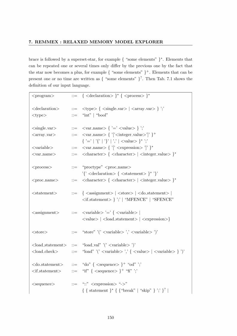
7. REMMEX : RELAXED MEMORY MODEL EXPLORER
brace is followed by a superset-star, for example “some elements” ∗. Elements that
can be repeated one or several times only differ by the previous one by the fact that
the star now becomes a plus, for example “some elements” +. Elements that can be
present one or no time are written as “some elements” ?. Then Tab. 7.1 shows the
definition of our input language.
<program> ::= <declaration> ∗ <process> ∗
<declaration> ::= <type> <single var> | <array var> ’;’
<type> ::= “int” | “bool”
<single var> ::= <var name> ’=’ <value> ’;’
<array var> ::= <var name> ’[’<integer value>’]’ +
’=’ | ’’ | ’’ | ’,’ | <value> ∗ ’;’
<variable> ::= <var name> ’[’ <expression> ’]’ ∗
<var name> ::= <character> <character> | <integer value> ∗
<process> ::= “proctype” <proc name>
’’ <declaration> <statement> ∗ ’’<proc name> ::= <character> <character> | <integer value> ∗
<statement> ::= <assignment> | <store> | <do statement> |<if statement> ’;’ | “MFENCE” | “SFENCE”
<assignment> ::= <variable> ’=’ <variable> |<value> | <load statement> | <expression>
<store> ::= “store” ’(’ <variable> ’,’ <variable> ’)’
<load statement> ::= “load val” ’(’ <variable> ’)’
<load check> ::= “load” ’(’ <variable> ’,’ <value> | <variable> ’)’
<do statement> ::= “do” <sequence> + “od” ’;’
<if statement> ::= “if” <sequence> + “fi” ’;’
<sequence> ::= “::” <expression> “->”
statement ∗ “break” | “skip” ’;’ ? |
150
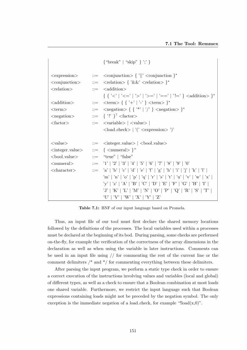
7.1 The Tool: Remmex
“break” | “skip” ’;’
<expression> ::= <conjunction> ’||’ <conjunction ∗
<conjunction> ::= <relation> ’&&’ <relation> ∗
<relation> ::= <addition>
’<’ | ’<=’ | ’>’ | ’>=’ | ’==’ | ’ !=’ <addition> ∗
<addition> ::= <term> ’+’ | ’-’ <term> ∗
<term> ::= <negation> ’*’ | ’/’ <negation> ∗
<negation> ::= ’ !’ ? <factor>
<factor> ::= <variable> | <value> |<load check> | ’(’ <expression> ’)’
<value> ::= <integer value> | <bool value>
<integer value> ::= <numeral> +
<bool value> ::= “true” | “false”
<numeral> ::= ’1’ | ’2’ | ’3’ | ’4’ | ’5’ | ’6’ | ’7’ | ’8’ | ’9’ | ’0’
<character> ::= ’a’ | ’b’ | ’c’ | ’d’ | ’e’ | ’f’ | ’g’ | ’h’ | ’i’ | ’j’ | ’k’ | ’l’ |’m’ | ’n’ | ’o’ | ’p’ | ’q’ | ’r’ | ’s’ | ’t’ | ’u’ | ’v’ | ’w’ | ’x’ |’y’ | ’z’ | ’A’ | ’B’ | ’C’ | ’D’ | ’E’ | ’F’ | ’G’ | ’H’ | ’I’ |’J’ | ’K’ | ’L’ | ’M’ | ’N’ | ’O’ | ’P’ | ’Q’ | ’R’ | ’S’ | ’T’ |’U’ | ’V’ | ’W’ | ’X’ | ’Y’ | ’Z’
Table 7.1: BNF of our input language based on Promela.
Thus, an input file of our tool must first declare the shared memory locations
followed by the definitions of the processes. The local variables used within a processes
must be declared at the beginning of its bod. During parsing, some checks are performed
on-the-fly, for example the verification of the correctness of the array dimensions in the
declaration as well as when using the variable in later instructions. Comments can
be used in an input file using // for commenting the rest of the current line or the
comment delimiters /* and */ for commenting everything between these delimiters.
After parsing the input program, we perform a static type check in order to ensure
a correct execution of the instructions involving values and variables (local and global)
of different types, as well as a check to ensure that a Boolean combination at most loads
one shared variable. Furthermore, we restrict the input language such that Boolean
expressions containing loads might not be preceded by the negation symbol. The only
exception is the immediate negation of a load check, for example “!load(x,0)”.
151
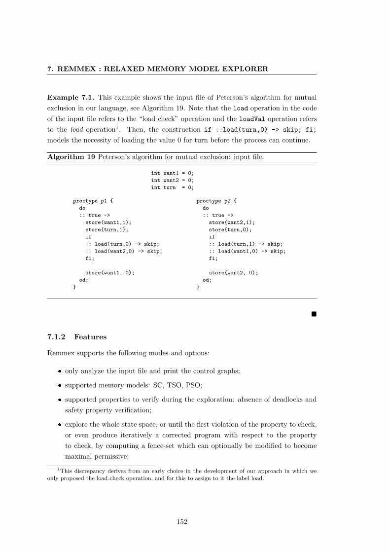
7. REMMEX : RELAXED MEMORY MODEL EXPLORER
Example 7.1. This example shows the input file of Peterson’s algorithm for mutual
exclusion in our language, see Algorithm 19. Note that the load operation in the code
of the input file refers to the “load check” operation and the loadVal operation refers
to the load operation1. Then, the construction if ::load(turn,0) -> skip; fi;
models the necessity of loading the value 0 for turn before the process can continue.
Algorithm 19 Peterson’s algorithm for mutual exclusion: input file.
int want1 = 0;
int want2 = 0;
int turn = 0;
proctype p1
do
:: true ->
store(want1,1);
store(turn,1);
if
:: load(turn,0) -> skip;
:: load(want2,0) -> skip;
fi;
store(want1, 0);
od;
proctype p2
do
:: true ->
store(want2,1);
store(turn,0);
if
:: load(turn,1) -> skip;
:: load(want1,0) -> skip;
fi;
store(want2, 0);
od;
7.1.2 Features
Remmex supports the following modes and options:
only analyze the input file and print the control graphs;
supported memory models: SC, TSO, PSO;
supported properties to verify during the exploration: absence of deadlocks and
safety property verification;
explore the whole state space, or until the first violation of the property to check,
or even produce iteratively a corrected program with respect to the property
to check, by computing a fence-set which can optionally be modified to become
maximal permissive;
1This discrepancy derives from an early choice in the development of our approach in which weonly proposed the load check operation, and for this to assign to it the label load.
152
7.1 The Tool: Remmex
print the state space, the store buffers or error-traces.
Note that all output files are written into the temporary directory of the current
system, and that “dot”-program is requested to be executable in the current location.
A second remark must be made with respect to the printed control graphs and the
state space. When using arrays, the printed control location does not take into account
the indexes to access a particular variable of an array. In the global state space, each
operation referring to a variable will print the index of the variable in the array. When
considering multi-dimensional arrays, the internal representation of the array flattens
the array and the indexes of a variable are transformed into a single index in the
flattened array. This also applies to simple variables, to which is concatenated the
index 0.
The man-page of the program is following, describing in details the features of
Remmex:
Usage: java remmex [Inputs] [Options]
Inputs:
*******-f The file to analyze
[requested]
-MM The memory model. Possible values: SC, TSO, PSO.
[Default: TSO]
-P The property to be checked. Possible values: safety , dead-
lock, controlgraphs. The option controlgraphs only analyzes
the syntax of the program and creates the control graphs.
[Default: safety]
-Mode The exploration mode. Possible values: firstError, allErrors,
errorCorrection, stateSpace.
[Default: errorCorrection]
-e Description of an error state (see below). Requested for
safety property check. There can be several error states.
Options:
********
153
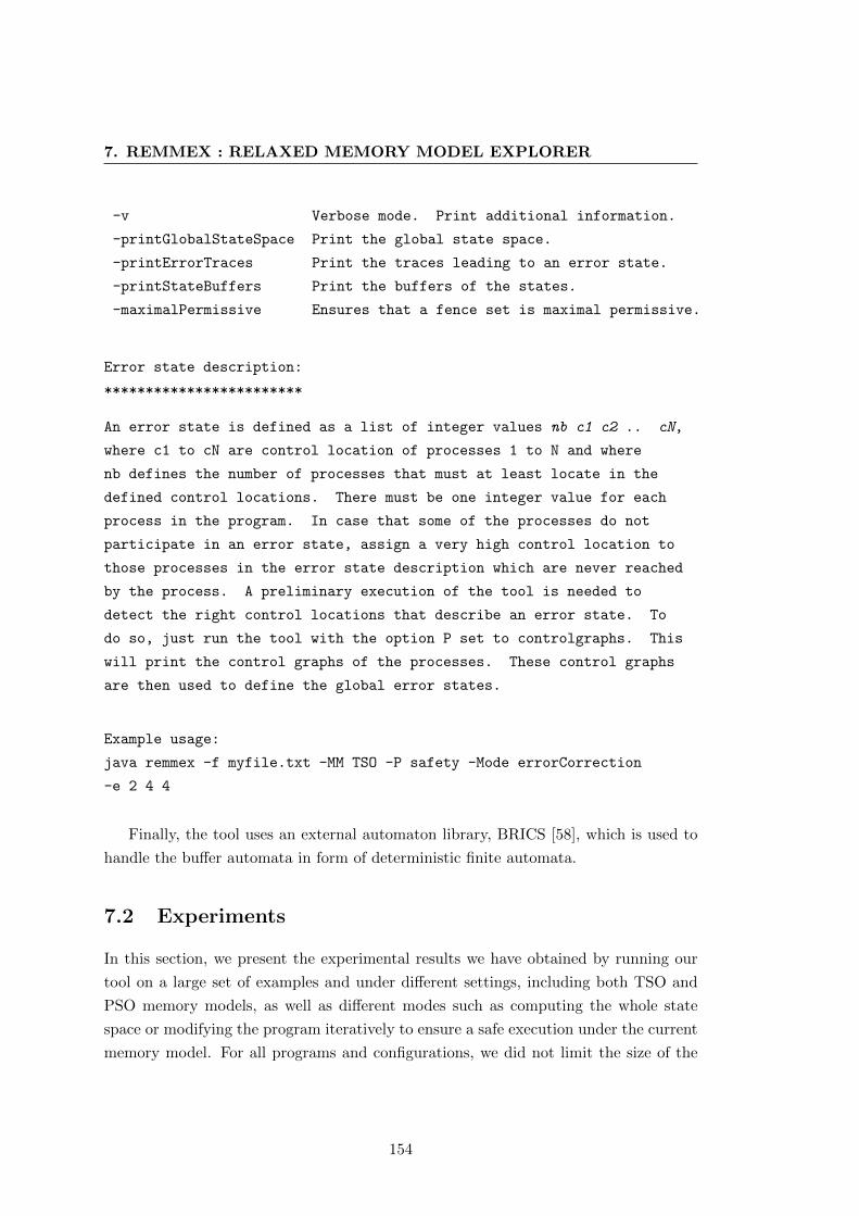
7. REMMEX : RELAXED MEMORY MODEL EXPLORER
-v Verbose mode. Print additional information.
-printGlobalStateSpace Print the global state space.
-printErrorTraces Print the traces leading to an error state.
-printStateBuffers Print the buffers of the states.
-maximalPermissive Ensures that a fence set is maximal permissive.
Error state description:
************************
An error state is defined as a list of integer values nb c1 c2 .. cN,
where c1 to cN are control location of processes 1 to N and where
nb defines the number of processes that must at least locate in the
defined control locations. There must be one integer value for each
process in the program. In case that some of the processes do not
participate in an error state, assign a very high control location to
those processes in the error state description which are never reached
by the process. A preliminary execution of the tool is needed to
detect the right control locations that describe an error state. To
do so, just run the tool with the option P set to controlgraphs. This
will print the control graphs of the processes. These control graphs
are then used to define the global error states.
Example usage:
java remmex -f myfile.txt -MM TSO -P safety -Mode errorCorrection
-e 2 4 4
Finally, the tool uses an external automaton library, BRICS [58], which is used to
handle the buffer automata in form of deterministic finite automata.
7.2 Experiments
In this section, we present the experimental results we have obtained by running our
tool on a large set of examples and under different settings, including both TSO and
PSO memory models, as well as different modes such as computing the whole state
space or modifying the program iteratively to ensure a safe execution under the current
memory model. For all programs and configurations, we did not limit the size of the
154
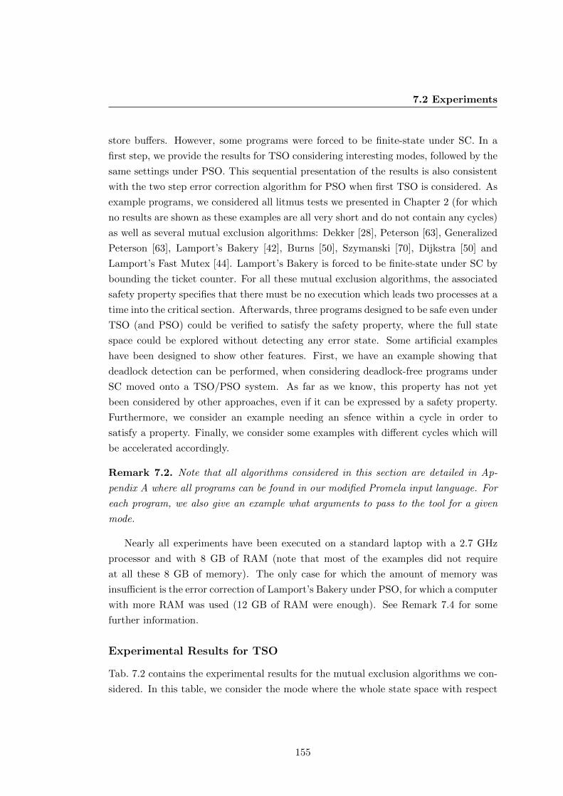
7.2 Experiments
store buffers. However, some programs were forced to be finite-state under SC. In a
first step, we provide the results for TSO considering interesting modes, followed by the
same settings under PSO. This sequential presentation of the results is also consistent
with the two step error correction algorithm for PSO when first TSO is considered. As
example programs, we considered all litmus tests we presented in Chapter 2 (for which
no results are shown as these examples are all very short and do not contain any cycles)
as well as several mutual exclusion algorithms: Dekker [28], Peterson [63], Generalized
Peterson [63], Lamport’s Bakery [42], Burns [50], Szymanski [70], Dijkstra [50] and
Lamport’s Fast Mutex [44]. Lamport’s Bakery is forced to be finite-state under SC by
bounding the ticket counter. For all these mutual exclusion algorithms, the associated
safety property specifies that there must be no execution which leads two processes at a
time into the critical section. Afterwards, three programs designed to be safe even under
TSO (and PSO) could be verified to satisfy the safety property, where the full state
space could be explored without detecting any error state. Some artificial examples
have been designed to show other features. First, we have an example showing that
deadlock detection can be performed, when considering deadlock-free programs under
SC moved onto a TSO/PSO system. As far as we know, this property has not yet
been considered by other approaches, even if it can be expressed by a safety property.
Furthermore, we consider an example needing an sfence within a cycle in order to
satisfy a property. Finally, we consider some examples with different cycles which will
be accelerated accordingly.
Remark 7.2. Note that all algorithms considered in this section are detailed in Ap-
pendix A where all programs can be found in our modified Promela input language. For
each program, we also give an example what arguments to pass to the tool for a given
mode.
Nearly all experiments have been executed on a standard laptop with a 2.7 GHz
processor and with 8 GB of RAM (note that most of the examples did not require
at all these 8 GB of memory). The only case for which the amount of memory was
insufficient is the error correction of Lamport’s Bakery under PSO, for which a computer
with more RAM was used (12 GB of RAM were enough). See Remark 7.4 for some
further information.
Experimental Results for TSO
Tab. 7.2 contains the experimental results for the mutual exclusion algorithms we con-
sidered. In this table, we consider the mode where the whole state space with respect
155
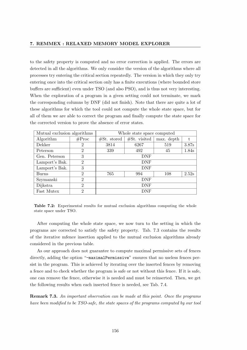
7. REMMEX : RELAXED MEMORY MODEL EXPLORER
to the safety property is computed and no error correction is applied. The errors are
detected in all the algorithms. We only consider the version of the algorithms where all
processes try entering the critical section repeatedly. The version in which they only try
entering once into the critical section only has a finite executions (where bounded store
buffers are sufficient) even under TSO (and also PSO), and is thus not very interesting.
When the exploration of a program in a given setting could not terminate, we mark
the corresponding columns by DNF (did not finish). Note that there are quite a lot of
these algorithms for which the tool could not compute the whole state space, but for
all of them we are able to correct the program and finally compute the state space for
the corrected version to prove the absence of error states.
Mutual exclusion algorithms Whole state space computed
Algorithm #Proc #St. stored #St. visited max. depth t
Dekker 2 3814 6267 519 3.87s
Peterson 2 339 492 45 1.84s
Gen. Peterson 3 DNF
Lamport’s Bak. 2 DNF
Lamport’s Bak. 3 DNF
Burns 2 765 994 108 2.52s
Szymanski 2 DNF
Dijkstra 2 DNF
Fast Mutex 2 DNF
Table 7.2: Experimental results for mutual exclusion algorithms computing the wholestate space under TSO.
After computing the whole state space, we now turn to the setting in which the
programs are corrected to satisfy the safety property. Tab. 7.3 contains the results
of the iterative mfence insertion applied to the mutual exclusion algorithms already
considered in the previous table.
As our approach does not guarantee to compute maximal permissive sets of fences
directly, adding the option “-maximalPermissive” ensures that no useless fences per-
sist in the program. This is achieved by iterating over the inserted fences by removing
a fence and to check whether the program is safe or not without this fence. If it is safe,
one can remove the fence, otherwise it is needed and must be reinserted. Then, we get
the following results when each inserted fence is needed, see Tab. 7.4.
Remark 7.3. An important observation can be made at this point. Once the programs
have been modified to be TSO-safe, the state spaces of the programs computed by our tool
156
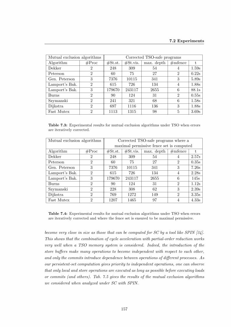
7.2 Experiments
Mutual exclusion algorithms Corrected TSO-safe programs
Algorithm #Proc #St.st. #St.vis. max. depth #mfence t
Dekker 2 248 309 54 4 1.59s
Peterson 2 60 75 27 2 0.22s
Gen. Peterson 3 7376 10115 341 3 5.89s
Lamport’s Bak. 2 615 726 134 4 1.88s
Lamport’s Bak. 3 179670 243117 2655 6 88.1s
Burns 2 90 124 31 2 0.55s
Szymanski 2 241 321 68 6 1.58s
Dijkstra 2 697 1116 136 3 1.88s
Fast Mutex 2 1113 1315 98 5 3.69s
Table 7.3: Experimental results for mutual exclusion algorithms under TSO when errorsare iteratively corrected.
Mutual exclusion algorithms Corrected TSO-safe programs where amaximal permissive fence set is computed
Algorithm #Proc #St.st. #St.vis. max. depth #mfence t
Dekker 2 248 309 54 4 2.57s
Peterson 2 60 75 27 2 0.35s
Gen. Peterson 3 7376 10115 341 3 7.26s
Lamport’s Bak. 2 615 726 134 4 2.28s
Lamport’s Bak. 3 179670 243117 2655 6 145s
Burns 2 90 124 31 2 1.12s
Szymanski 2 228 308 62 3 2.39s
Dijkstra 2 769 1272 149 2 3.35s
Fast Mutex 2 1207 1465 97 4 4.33s
Table 7.4: Experimental results for mutual exclusion algorithms under TSO when errorsare iteratively corrected and where the fence set is ensured to be maximal permissive.
become very close in size as those that can be computed for SC by a tool like SPIN [34].
This shows that the combination of cycle acceleration with partial-order reduction works
very well when a TSO memory system is considered. Indeed, the introduction of the
store buffers make many operations to become independent with respect to each other,
and only the commits introduce dependence between operations of different processes. As
our persistent-set computation gives priority to independent operations, one can observe
that only local and store operations are executed as long as possible before executing loads
or commits (and others). Tab. 7.5 gives the results of the mutual exclusion algorithms
we considered when analyzed under SC with SPIN.
157
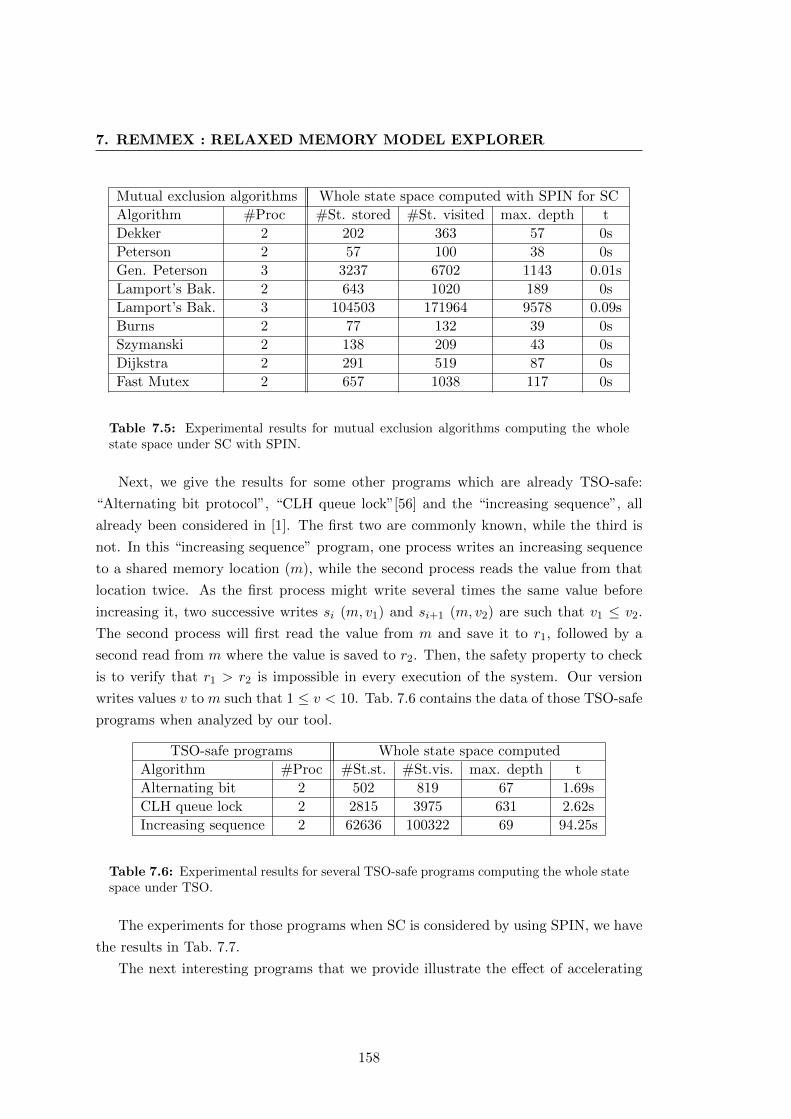
7. REMMEX : RELAXED MEMORY MODEL EXPLORER
Mutual exclusion algorithms Whole state space computed with SPIN for SC
Algorithm #Proc #St. stored #St. visited max. depth t
Dekker 2 202 363 57 0s
Peterson 2 57 100 38 0s
Gen. Peterson 3 3237 6702 1143 0.01s
Lamport’s Bak. 2 643 1020 189 0s
Lamport’s Bak. 3 104503 171964 9578 0.09s
Burns 2 77 132 39 0s
Szymanski 2 138 209 43 0s
Dijkstra 2 291 519 87 0s
Fast Mutex 2 657 1038 117 0s
Table 7.5: Experimental results for mutual exclusion algorithms computing the wholestate space under SC with SPIN.
Next, we give the results for some other programs which are already TSO-safe:
“Alternating bit protocol”, “CLH queue lock”[56] and the “increasing sequence”, all
already been considered in [1]. The first two are commonly known, while the third is
not. In this “increasing sequence” program, one process writes an increasing sequence
to a shared memory location (m), while the second process reads the value from that
location twice. As the first process might write several times the same value before
increasing it, two successive writes si (m, v1) and si+1 (m, v2) are such that v1 ≤ v2.
The second process will first read the value from m and save it to r1, followed by a
second read from m where the value is saved to r2. Then, the safety property to check
is to verify that r1 > r2 is impossible in every execution of the system. Our version
writes values v to m such that 1 ≤ v < 10. Tab. 7.6 contains the data of those TSO-safe
programs when analyzed by our tool.
TSO-safe programs Whole state space computed
Algorithm #Proc #St.st. #St.vis. max. depth t
Alternating bit 2 502 819 67 1.69s
CLH queue lock 2 2815 3975 631 2.62s
Increasing sequence 2 62636 100322 69 94.25s
Table 7.6: Experimental results for several TSO-safe programs computing the whole statespace under TSO.
The experiments for those programs when SC is considered by using SPIN, we have
the results in Tab. 7.7.
The next interesting programs that we provide illustrate the effect of accelerating
158
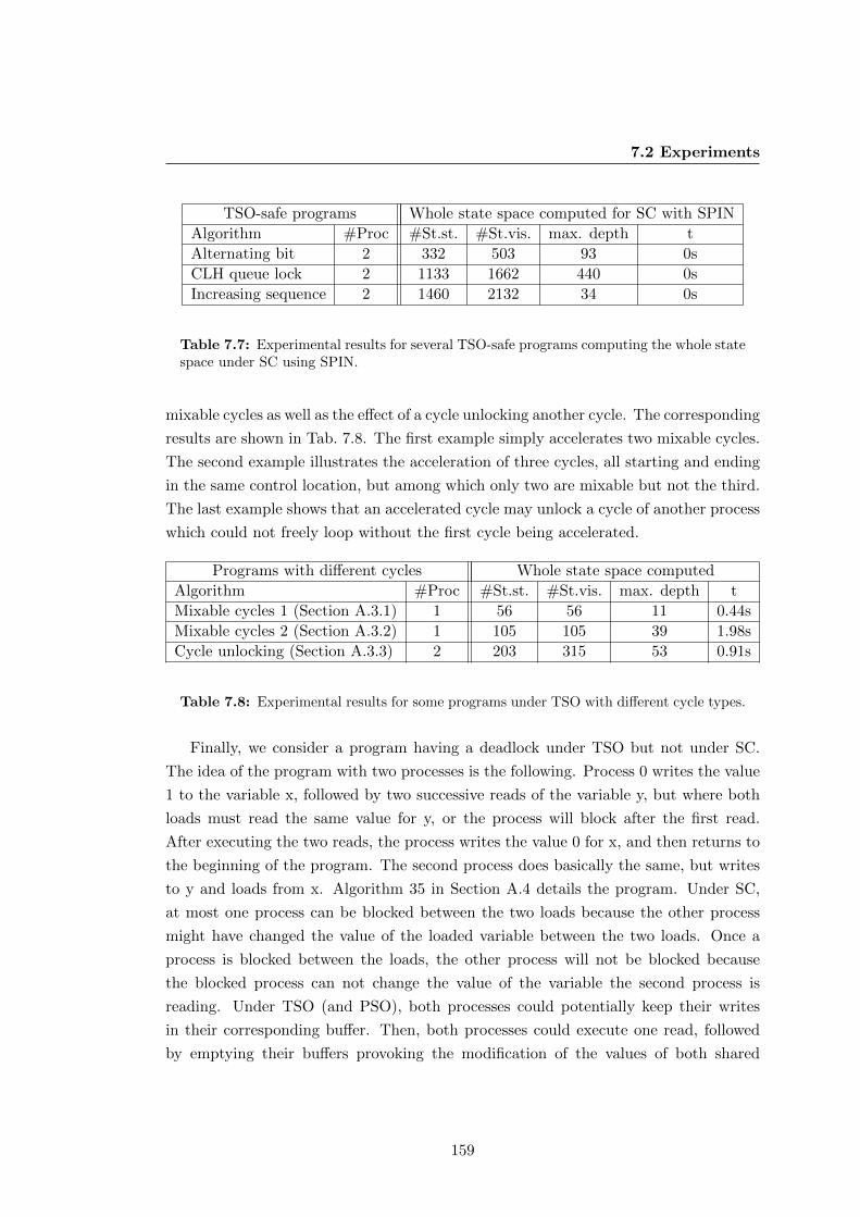
7.2 Experiments
TSO-safe programs Whole state space computed for SC with SPIN
Algorithm #Proc #St.st. #St.vis. max. depth t
Alternating bit 2 332 503 93 0s
CLH queue lock 2 1133 1662 440 0s
Increasing sequence 2 1460 2132 34 0s
Table 7.7: Experimental results for several TSO-safe programs computing the whole statespace under SC using SPIN.
mixable cycles as well as the effect of a cycle unlocking another cycle. The corresponding
results are shown in Tab. 7.8. The first example simply accelerates two mixable cycles.
The second example illustrates the acceleration of three cycles, all starting and ending
in the same control location, but among which only two are mixable but not the third.
The last example shows that an accelerated cycle may unlock a cycle of another process
which could not freely loop without the first cycle being accelerated.
Programs with different cycles Whole state space computed
Algorithm #Proc #St.st. #St.vis. max. depth t
Mixable cycles 1 (Section A.3.1) 1 56 56 11 0.44s
Mixable cycles 2 (Section A.3.2) 1 105 105 39 1.98s
Cycle unlocking (Section A.3.3) 2 203 315 53 0.91s
Table 7.8: Experimental results for some programs under TSO with different cycle types.
Finally, we consider a program having a deadlock under TSO but not under SC.
The idea of the program with two processes is the following. Process 0 writes the value
1 to the variable x, followed by two successive reads of the variable y, but where both
loads must read the same value for y, or the process will block after the first read.
After executing the two reads, the process writes the value 0 for x, and then returns to
the beginning of the program. The second process does basically the same, but writes
to y and loads from x. Algorithm 35 in Section A.4 details the program. Under SC,
at most one process can be blocked between the two loads because the other process
might have changed the value of the loaded variable between the two loads. Once a
process is blocked between the loads, the other process will not be blocked because
the blocked process can not change the value of the variable the second process is
reading. Under TSO (and PSO), both processes could potentially keep their writes
in their corresponding buffer. Then, both processes could execute one read, followed
by emptying their buffers provoking the modification of the values of both shared
159
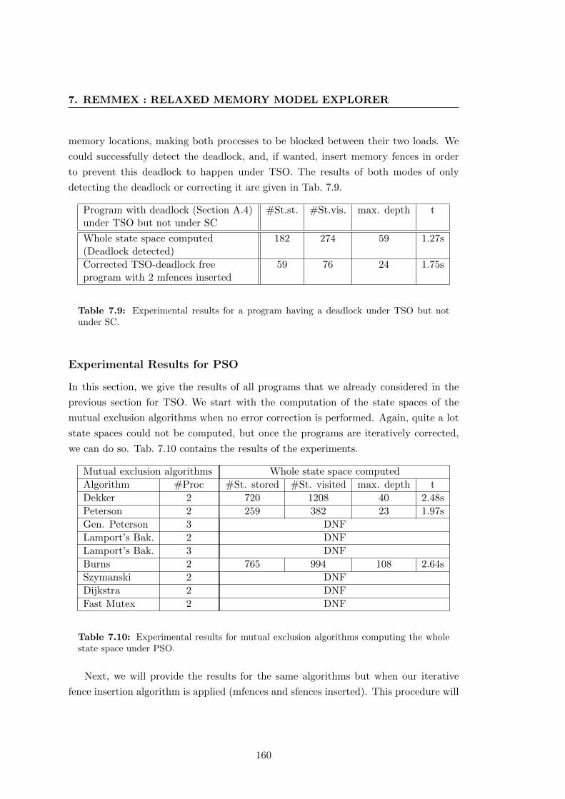
7. REMMEX : RELAXED MEMORY MODEL EXPLORER
memory locations, making both processes to be blocked between their two loads. We
could successfully detect the deadlock, and, if wanted, insert memory fences in order
to prevent this deadlock to happen under TSO. The results of both modes of only
detecting the deadlock or correcting it are given in Tab. 7.9.
Program with deadlock (Section A.4) #St.st. #St.vis. max. depth tunder TSO but not under SC
Whole state space computed 182 274 59 1.27s(Deadlock detected)
Corrected TSO-deadlock free 59 76 24 1.75sprogram with 2 mfences inserted
Table 7.9: Experimental results for a program having a deadlock under TSO but notunder SC.
Experimental Results for PSO
In this section, we give the results of all programs that we already considered in the
previous section for TSO. We start with the computation of the state spaces of the
mutual exclusion algorithms when no error correction is performed. Again, quite a lot
state spaces could not be computed, but once the programs are iteratively corrected,
we can do so. Tab. 7.10 contains the results of the experiments.
Mutual exclusion algorithms Whole state space computed
Algorithm #Proc #St. stored #St. visited max. depth t
Dekker 2 720 1208 40 2.48s
Peterson 2 259 382 23 1.97s
Gen. Peterson 3 DNF
Lamport’s Bak. 2 DNF
Lamport’s Bak. 3 DNF
Burns 2 765 994 108 2.64s
Szymanski 2 DNF
Dijkstra 2 DNF
Fast Mutex 2 DNF
Table 7.10: Experimental results for mutual exclusion algorithms computing the wholestate space under PSO.
Next, we will provide the results for the same algorithms but when our iterative
fence insertion algorithm is applied (mfences and sfences inserted). This procedure will
160
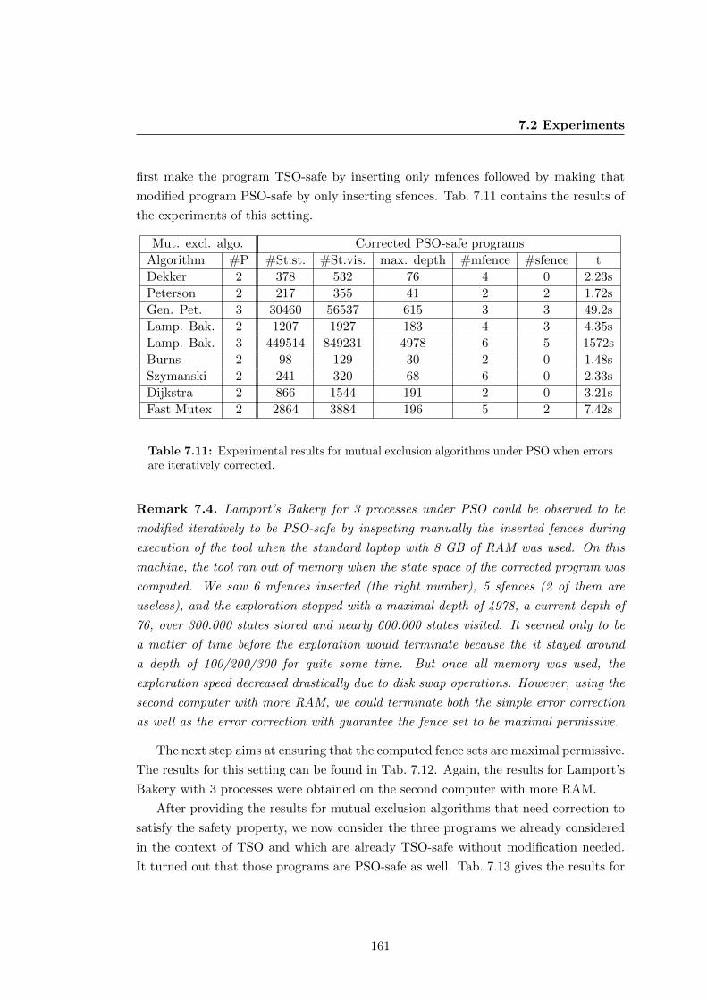
7.2 Experiments
first make the program TSO-safe by inserting only mfences followed by making that
modified program PSO-safe by only inserting sfences. Tab. 7.11 contains the results of
the experiments of this setting.
Mut. excl. algo. Corrected PSO-safe programs
Algorithm #P #St.st. #St.vis. max. depth #mfence #sfence t
Dekker 2 378 532 76 4 0 2.23s
Peterson 2 217 355 41 2 2 1.72s
Gen. Pet. 3 30460 56537 615 3 3 49.2s
Lamp. Bak. 2 1207 1927 183 4 3 4.35s
Lamp. Bak. 3 449514 849231 4978 6 5 1572s
Burns 2 98 129 30 2 0 1.48s
Szymanski 2 241 320 68 6 0 2.33s
Dijkstra 2 866 1544 191 2 0 3.21s
Fast Mutex 2 2864 3884 196 5 2 7.42s
Table 7.11: Experimental results for mutual exclusion algorithms under PSO when errorsare iteratively corrected.
Remark 7.4. Lamport’s Bakery for 3 processes under PSO could be observed to be
modified iteratively to be PSO-safe by inspecting manually the inserted fences during
execution of the tool when the standard laptop with 8 GB of RAM was used. On this
machine, the tool ran out of memory when the state space of the corrected program was
computed. We saw 6 mfences inserted (the right number), 5 sfences (2 of them are
useless), and the exploration stopped with a maximal depth of 4978, a current depth of
76, over 300.000 states stored and nearly 600.000 states visited. It seemed only to be
a matter of time before the exploration would terminate because the it stayed around
a depth of 100/200/300 for quite some time. But once all memory was used, the
exploration speed decreased drastically due to disk swap operations. However, using the
second computer with more RAM, we could terminate both the simple error correction
as well as the error correction with guarantee the fence set to be maximal permissive.
The next step aims at ensuring that the computed fence sets are maximal permissive.
The results for this setting can be found in Tab. 7.12. Again, the results for Lamport’s
Bakery with 3 processes were obtained on the second computer with more RAM.
After providing the results for mutual exclusion algorithms that need correction to
satisfy the safety property, we now consider the three programs we already considered
in the context of TSO and which are already TSO-safe without modification needed.
It turned out that those programs are PSO-safe as well. Tab. 7.13 gives the results for
161
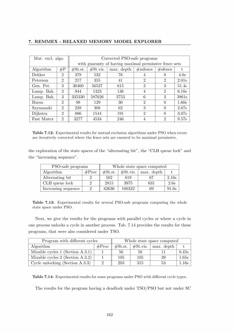
7. REMMEX : RELAXED MEMORY MODEL EXPLORER
Mut. excl. algo. Corrected PSO-safe programswith guaranty of having maximal permissive fence sets
Algorithm #P #St.st. #St.vis. max. depth #mfence #sfence t
Dekker 2 378 532 76 4 0 4.0s
Peterson 2 217 355 41 2 2 2.01s
Gen. Pet. 3 30460 56537 615 3 3 51.4s
Lamp. Bak. 2 944 1323 136 4 2 6.10s
Lamp. Bak. 3 335330 587626 3753 6 3 3861s
Burns 2 98 129 30 2 0 1.60s
Szymanski 2 228 308 62 3 0 2.67s
Dijkstra 2 866 1544 191 2 0 3.07s
Fast Mutex 2 3277 4534 246 4 2 9.57s
Table 7.12: Experimental results for mutual exclusion algorithms under PSO when errorsare iteratively corrected where the fence sets are ensured to be maximal permissive.
the exploration of the state spaces of the “alternating bit”, the “CLH queue lock” and
the “increasing sequence”.
PSO-safe programs Whole state space computed
Algorithm #Proc #St.st. #St.vis. max. depth t
Alternating bit 2 502 819 67 2.16s
CLH queue lock 2 2815 3975 631 2.6s
Increasing sequence 2 62636 100322 69 91.6s
Table 7.13: Experimental results for several PSO-safe programs computing the wholestate space under PSO.
Next, we give the results for the programs with parallel cycles or where a cycle in
one process unlocks a cycle in another process. Tab. 7.14 provides the results for these
programs, that were also considered under TSO.
Program with different cycles Whole state space computed
Algorithm #Proc #St.st. #St.vis. max. depth t
Mixable cycles 1 (Section A.3.1) 1 56 56 11 0.45s
Mixable cycles 2 (Section A.3.2) 1 105 105 39 1.65s
Cycle unlocking (Section A.3.3) 2 203 315 53 1.16s
Table 7.14: Experimental results for some programs under PSO with different cycle types.
The results for the program having a deadlock under TSO/PSO but not under SC
162
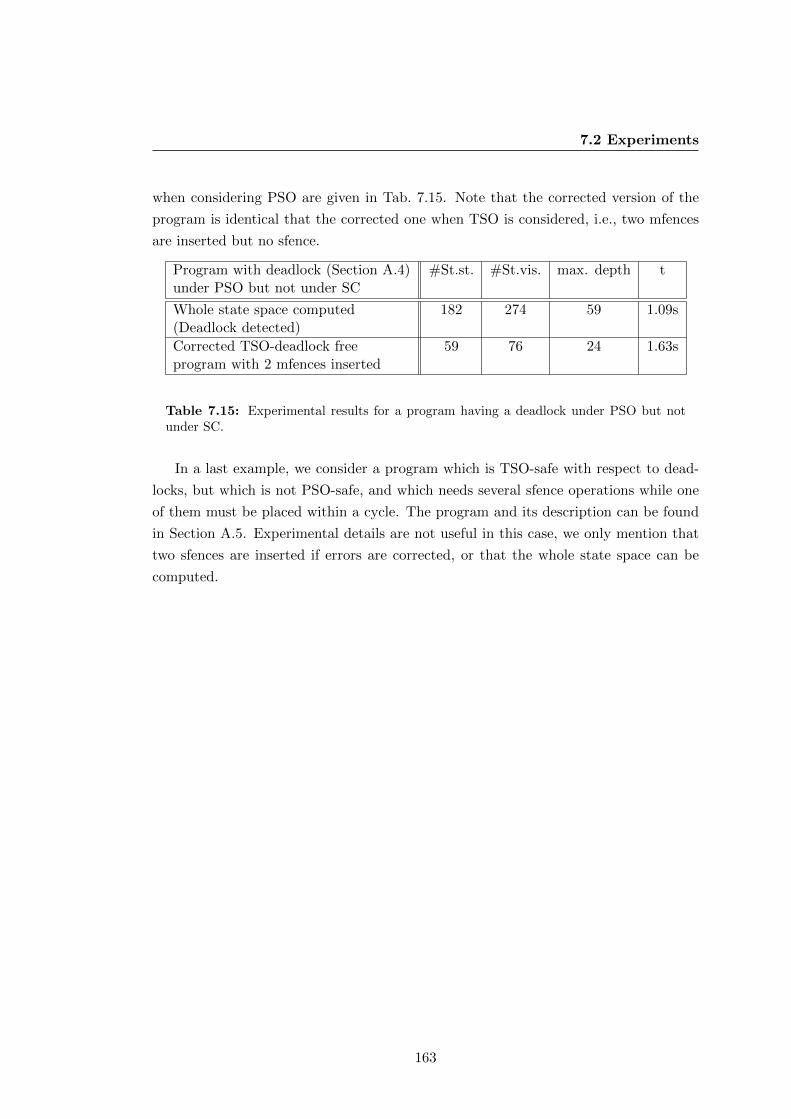
7.2 Experiments
when considering PSO are given in Tab. 7.15. Note that the corrected version of the
program is identical that the corrected one when TSO is considered, i.e., two mfences
are inserted but no sfence.
Program with deadlock (Section A.4) #St.st. #St.vis. max. depth tunder PSO but not under SC
Whole state space computed 182 274 59 1.09s(Deadlock detected)
Corrected TSO-deadlock free 59 76 24 1.63sprogram with 2 mfences inserted
Table 7.15: Experimental results for a program having a deadlock under PSO but notunder SC.
In a last example, we consider a program which is TSO-safe with respect to dead-
locks, but which is not PSO-safe, and which needs several sfence operations while one
of them must be placed within a cycle. The program and its description can be found
in Section A.5. Experimental details are not useful in this case, we only mention that
two sfences are inserted if errors are corrected, or that the whole state space can be
computed.
163

Chapter 8
Conclusions
8.1 Summary
The main result of this work is an original approach to handle the problem of exploring
the state space of concurrent programs that are finite-state under the classical sequential
consistency memory model, but become infinite-state when executed under relaxed
memory models. This is due to the unbounded buffers that are added to the system in
order to correctly model these memory systems. As most current processors implement
relaxed memory models instead of the traditional strong memory model, the approach
can help software developers to design programs intended to be executed on modern
processors. The two memory models that have been considered are Total Store Order
(TSO) and Partial Store Order (PSO). While TSO is widely used these days on current
x86 processors, PSO is not actually implemented as such, but represents a subset of
other memory models that are currently implemented on processors. A large set of
processors are thus covered by our approach, which can thus be widely used.
The proposed approach extends classical state-space exploration algorithms in order
to allow the exploration of infinite state spaces of programs when executed under a
relaxed memory system, and can be combined with the state-space reduction techniques
known as partial-order reduction techniques, which aim at reducing the size of the state
space by exploiting independence of transitions. The approach thus proposes a solution
to the state-reachability problem by exploring and constructing the state space, allowing
the verification of absence of deadlocks and the verification of safety properties.
The main idea underlying our approach is to recognize a special type of cycles in
the program during the exploration of the state space and to compute the effect of
the repeated execution of such a cycle in the form of a symbolic state representing all
165
8. CONCLUSIONS
states reachable after any number of iterations of the cycle. This is what we call “cycle
acceleration”. Moreover, we support the acceleration of parallel cycles under some
conditions, computing a symbolic state representing all states reachable by repeatedly
executing these parallel cycles. When using cycle acceleration, we relinquish guaranteed
termination, because the construction of the state space is undecidable in general in
the context of the memory systems we consider. However, in many of our experiments,
the exploration of the state space of the system was successful.
The introduction of the store buffers into the system has an important impact on
the notion of independence between the operations of the system. Indeed, all memory
write operations are not executed on the shared memory, but on the store buffers which
are exclusively associated to a particular process. By doing so, they can be considered
to be local operations with respect to independence. When considering partial-order
reduction techniques, a greater set of pairs of independent transitions implies a bigger
reduction of the state space, while preserving enough interleavings to correctly verify
a given property (absence of deadlocks or safety properties), but removing many other
interleavings leading to the same state, which only differ by the order of independent
transitions. By combining cycle acceleration with partial-order reduction, we achieve
a strong reduction of the state space. For programs that are correct with respect to
safety properties, the size of the state space we compute is, in most cases (and of course
depending on the program), not much different from the size of the state space for the
same program when it is analyzed under SC with the model-checker SPIN. From an
outside point of view, this might seem strange because of the addition of the store
buffer components to the system and thus of more possible behaviors, but once one
has understood that these buffers introduce a lot of independence, it become quite
obvious why partial-order reductions work even better with the store buffers present
under TSO/PSO than under SC where no store buffers are present.
Our second contribution is to propose a technique to ensure that a program preserves
a given property when it is moved onto a relaxed memory system. This is done by
selecting places in the program where special synchronization operations are added in
order to remove the possibility of reaching states violating the property.
All these results have been published in [45, 46, 47].
8.2 Related Work
The emergence of multi-core processors implementing weak memory models has moti-
vated the development of several different approaches for verifying programs executed
166
8.2 Related Work
on these processors. Simultaneously, there is also a lot of research work about formally
defining the memory models of commercial processors, vendors not providing more than
an informal description and allowed/disallowed execution scenarios.
Since, the verification approaches only became possible after the formal definition
of the memory models, we start with briefly giving an overview over the work that
has been done in this area. The memory model x86-TSO has been defined in [60, 65],
which concurs with the informal definition of x86-processors, and which is the basis
for all work dealing the TSO memory model. Besides, more theoretical work on the
differences between memory models from an axiomatic view was given in [54]. In
this work, the number of litmus tests needed to specify a memory model are set into
relation with the different memory models. In later work, an axiomatic memory model
was presented for POWER multiprocessors, [55]. Two more interesting studies on
the decidability/undecidability of the verification of programs under relaxed memory
models appear in [11, 12]. In these papers, the focus was to inspect which relaxations
influence the decidability of different properties. It turns out that store buffering under
TSO/PSO does not make state-reachability undecidable. It follows that any safety
property verification is decidable. However, computing the whole state space becomes
undecidable under these settings, as well as the repeated-reachability, which is needed
for liveness properties. All those results are obtained by simulating TSO/PSO-systems
by lossy channel systems (LCS) and vice-versa. This simulations makes all results for
LCS also hold for TSO/PSO-systems. Finally, the most relaxed memory model for
which state-reachability is decidable has been proposed. It is the one allowing the
store-store, store-load and load-load relaxations. Adding the load-store relaxation is
shown to be the crucial element that makes state-reachability undecidable.
Now, we focus on the closely related approaches with respect to the verification of
programs and the preservation of properties by fence insertion. The different techniques
can be divided into two main streams: Verifying the program with respect to a given
property by modeling the store buffers in some way and trying to only disable by
fence insertion the traces leading to a state violating the property, or to analyze the
programs focusing on SC, while looking for causes that can turn an SC-execution into
a, for example, TSO-execution by allowing the order of operations to be changed, which
is know under the name of the robustness-question or the stability-question. It follows
that the first type of approaches will likely insert less fences than the second type, while
the first type should scale better, because much less behaviors will be checked. We will
only compare our approach in detail to those that are close enough in terms of the
technique that is used and will only outline the others.
167
8. CONCLUSIONS
A first approach with respect to state-reachability and fence-set computation for
safety property preservation when TSO is considered instead of SC has emerged from
the bidirectional simulation of TSO and LCS (lossy channel systems) of [11]. In [1], the
approach is used to prove the decidability of state-reachability by exploiting the results
for LCS. The algorithm works by exploring the state space backwards, starting from a
given state and checking if the initial state of the system is reachable. Since an effective
algorithm exists for LCS, it could be transcribed for TSO-systems, where one can check
if a given error-state can be reached. Alongside, an algorithm for computing all maximal
permissive fence sets is provided when safety property preservation is considered. The
algorithm works by building step-by-step (or error trace by error trace) different fence
sets, while ensuring that there never are two fence sets such that one is included in
the other. This ensures that all computed fence sets will be maximal permissive. The
fence sets we compute are consistent with those obtained by this approach. Also note
that the procedure to compute the fence sets can be combined with our state-space
exploration technique, because it is based on traces leading to error states, which is
also performed by our approach. The advantage of our approach is that it proceeds
more naturally by exploring the state space forwards, while their approach explores
backwards, which might lead the exploration to intermediate states which cannot be
reached by the program. Another advantage of our approach is that we can easily verify
the absence of deadlocks, while for their approach, a huge number of “bad-states” must
be considered, from each of which they must perform their backwards search. As far as
we know, they do not consider the detection of deadlocks. All those results have been
implemented in a tool presented in [2].
A second approach has been presented in [40, 41], where the memory models TSO,
PSO and a simplified RMO are considered. In the first paper, a fence inference tech-
nique has been proposed: it works by propagating through the state space constraints
that represent relaxations that could be removed by a fence. Once an undesirable state
is reached, one can use the associated constraints in order to determine how to make
that state unreachable for all incoming paths. In the second paper, an over-abstraction
technique for the buffer representation has been introduced in order to also allow the
verification of programs with infinite executions, i.e., programs having cycles, and thus
making the exploration of the state space possible under this setting. This technique
has been successfully combined with the fence inference technique, but suffer from two
disadvantages. The first disadvantage is that they can reach states which are identified
to be “bad-states” but that are not reachable by the program, but where the abstraction
technique made the exploration loose too much information about the buffer content.
168
8.2 Related Work
The second disadvantage also results from the abstraction of the store buffer, which
can lead to an explosion of the size of the state spaces being computed even for small
programs, making it impossible to compute any fence set. For example, Lamport’s
“Fast Mutex” is out of reach of this method, if a first fence is not manually inserted
before running the tool. A version of the CLH queue lock could also not be handled
due to the size of the state space, but it is unclear if their version of this program and
ours are the same. Also, the increasing sequence example cannot be verified at all by
their approach. For all programs that both our and their approach can handle, and
for which no manual fence insertion was done, the computed fences are the same. The
problem of the size of the state spaces has been addressed in [48] of the same authors,
where an iterative version of the previous work is proposed. In this version, instead
of computing the whole state space directly with all error states, they stop when the
first error state is reached. Once such an error state is reached, the user might decide
between directly correcting the program, accumulating more error traces or other pos-
sibilities. This approach can be viewed as an adaptation of our iterative fence insertion
technique to their approach.
We continue by reviewing the works in the spirit of robustness or stability, meaning
that a program is robust or stable with respect to a given memory model if, when it
is moved to that memory model, all executions remain compatible with SC-executions.
For example, a program is TSO-robust if it only allows SC-execution even when the
underlying memory system is TSO. Those approaches scale better because there is no
need to model the unbounded store buffers. An interesting work is [21], where it is
shown that there are always minimal violating computations that relaxes the order of
two instructions in a single process. These results are exploited in [20] to build a tool
which computes minimal fence sets with respect to TSO-robustness. Other work in
the same directions are [8, 9, 10] or [23], all based on the happens-before relation given
in [66].
Other related work is given in [14, 22, 24, 29, 33, 35, 36, 39, 49, 51, 52, 59, 61, 64].
Last but not least, we must mention some work from which we have taken ideas or
results. This includes the concept of meta-transitions and the exploration of infinite
state spaces presented in [15, 16, 17, 18, 19, 72], where meta-transitions also aim at
computing the effect of the repeated execution of a given cycle (or a set of cycles) in
a single step. Next, we widely used the partial-order reduction techniques presented
in [31], as well as concepts introduced in [71] for computing Stubborn-sets, which were
proved to be persistent-sets with respect to the definitions in [31].
169
8. CONCLUSIONS
8.3 Future Work
There are several possible directions for future work. Five of them are broad extensions
or future directions, the others only aim at optimizing the current approach.
The first broad future work would be to consider programs that do not have a
limited memory domain, and where the approach is combined with an abstraction
technique in order to handle infinite data domain. This already has been considered
in [27] extending the work of [41]. A similar work has been proposed earlier in [1]. The
implementation of [11] in [2] also already proposes to use an abstraction technique in
order to allow unbounded data handling.
The second broad direction for future work is to analyze whether it is possible
to make use of our approach when considering other memory models, such as IBM’s
PowerPC or ARM architectures, or to analyze if it would be possible to combine our
approach with one of approaches in the robustness-family.
Another future direction would be to combine our approach with an over-appro-
ximation approach, in order to force the computed state space to stay finite. This
could be done by representing the buffer contents using a smart combination of buffer
automata and unordered sets. This approach would then allow the computation of the
state space of finite-state programs having any type of cycles.
The next direction for future work would be to make an analysis of the classes
of cycles that can be represented by buffer automata. Conversely, one could analyze
whether a simpler representation would be sufficient for most types of cycles.
The last direction for future work aims at almost any approach that addresses
the verification of programs on relaxed memory models: the problem of parametric
verification. For example, given that there is a corrected version of Lamport’s Bakery
under TSO (“LB-TSO”) for K processes, and given that one can proof that Lamport’s
Bakery under SO verified for K processes generalizes to N > K processes under SC,
can one conclude that “LB-TSO” generalizes to N processes under TSO?
Less important future work include the optimization of the partial-order reduction
technique that is used, and the optimization, or generalization, of the types of cycles
that can be detected by the approach, and other small improvements.
170
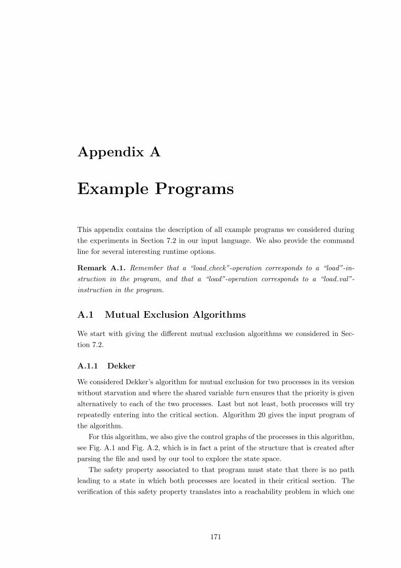
Appendix A
Example Programs
This appendix contains the description of all example programs we considered during
the experiments in Section 7.2 in our input language. We also provide the command
line for several interesting runtime options.
Remark A.1. Remember that a “load check”-operation corresponds to a “load”-in-
struction in the program, and that a “load”-operation corresponds to a “load val”-
instruction in the program.
A.1 Mutual Exclusion Algorithms
We start with giving the different mutual exclusion algorithms we considered in Sec-
tion 7.2.
A.1.1 Dekker
We considered Dekker’s algorithm for mutual exclusion for two processes in its version
without starvation and where the shared variable turn ensures that the priority is given
alternatively to each of the two processes. Last but not least, both processes will try
repeatedly entering into the critical section. Algorithm 20 gives the input program of
the algorithm.
For this algorithm, we also give the control graphs of the processes in this algorithm,
see Fig. A.1 and Fig. A.2, which is in fact a print of the structure that is created after
parsing the file and used by our tool to explore the state space.
The safety property associated to that program must state that there is no path
leading to a state in which both processes are located in their critical section. The
verification of this safety property translates into a reachability problem in which one
171
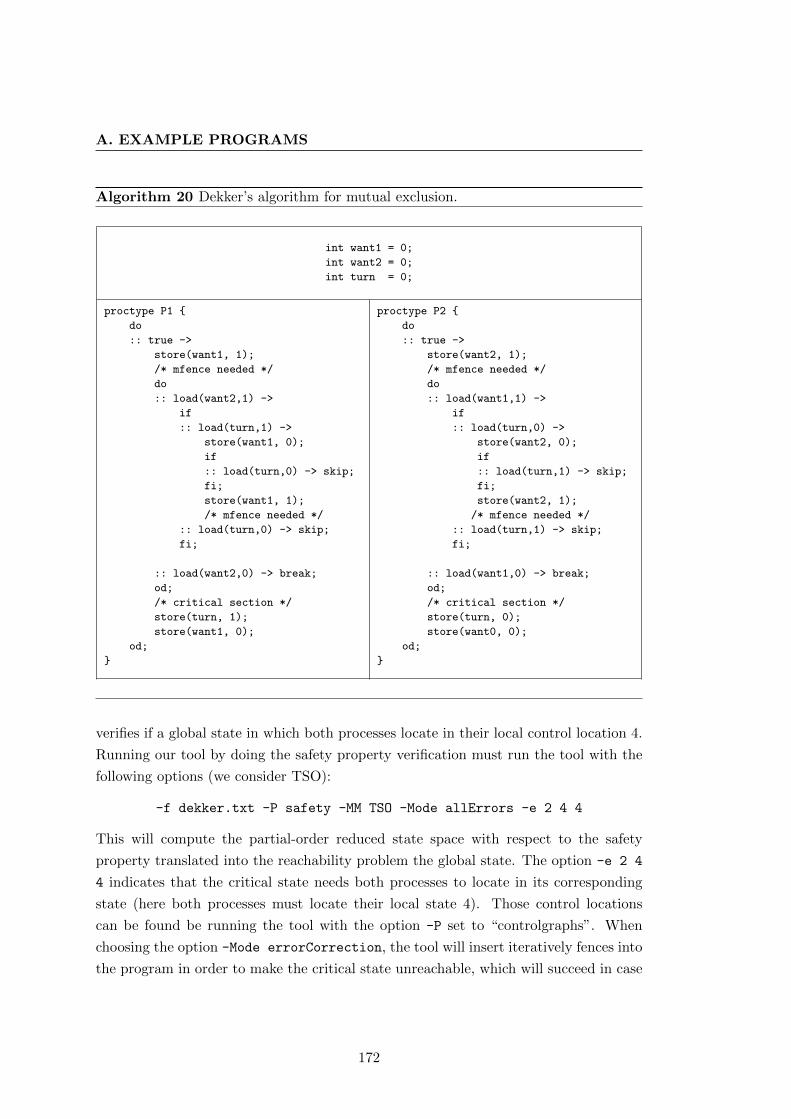
A. EXAMPLE PROGRAMS
Algorithm 20 Dekker’s algorithm for mutual exclusion.
int want1 = 0;
int want2 = 0;
int turn = 0;
proctype P1
do
:: true ->
store(want1, 1);
/* mfence needed */
do
:: load(want2,1) ->
if
:: load(turn,1) ->
store(want1, 0);
if
:: load(turn,0) -> skip;
fi;
store(want1, 1);
/* mfence needed */
:: load(turn,0) -> skip;
fi;
:: load(want2,0) -> break;
od;
/* critical section */
store(turn, 1);
store(want1, 0);
od;
proctype P2
do
:: true ->
store(want2, 1);
/* mfence needed */
do
:: load(want1,1) ->
if
:: load(turn,0) ->
store(want2, 0);
if
:: load(turn,1) -> skip;
fi;
store(want2, 1);
/* mfence needed */
:: load(turn,1) -> skip;
fi;
:: load(want1,0) -> break;
od;
/* critical section */
store(turn, 0);
store(want0, 0);
od;
verifies if a global state in which both processes locate in their local control location 4.
Running our tool by doing the safety property verification must run the tool with the
following options (we consider TSO):
-f dekker.txt -P safety -MM TSO -Mode allErrors -e 2 4 4
This will compute the partial-order reduced state space with respect to the safety
property translated into the reachability problem the global state. The option -e 2 4
4 indicates that the critical state needs both processes to locate in its corresponding
state (here both processes must locate their local state 4). Those control locations
can be found be running the tool with the option -P set to “controlgraphs”. When
choosing the option -Mode errorCorrection, the tool will insert iteratively fences into
the program in order to make the critical state unreachable, which will succeed in case
172
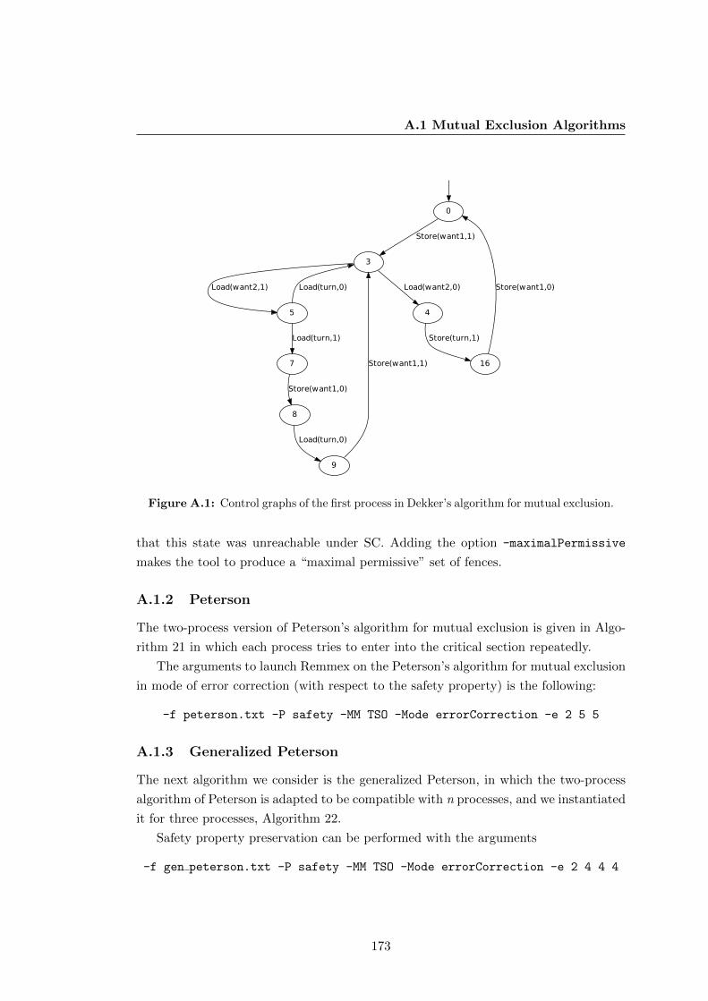
A.1 Mutual Exclusion Algorithms
0
3
Store(want1,1)
5
Load(want2,1)
4
Load(want2,0)Load(turn,0)
7
Load(turn,1)
16
Store(turn,1)
Store(want1,0)
8
Store(want1,0)
9
Load(turn,0)
Store(want1,1)
Figure A.1: Control graphs of the first process in Dekker’s algorithm for mutual exclusion.
that this state was unreachable under SC. Adding the option -maximalPermissive
makes the tool to produce a “maximal permissive” set of fences.
A.1.2 Peterson
The two-process version of Peterson’s algorithm for mutual exclusion is given in Algo-
rithm 21 in which each process tries to enter into the critical section repeatedly.
The arguments to launch Remmex on the Peterson’s algorithm for mutual exclusion
in mode of error correction (with respect to the safety property) is the following:
-f peterson.txt -P safety -MM TSO -Mode errorCorrection -e 2 5 5
A.1.3 Generalized Peterson
The next algorithm we consider is the generalized Peterson, in which the two-process
algorithm of Peterson is adapted to be compatible with n processes, and we instantiated
it for three processes, Algorithm 22.
Safety property preservation can be performed with the arguments
-f gen peterson.txt -P safety -MM TSO -Mode errorCorrection -e 2 4 4 4
173
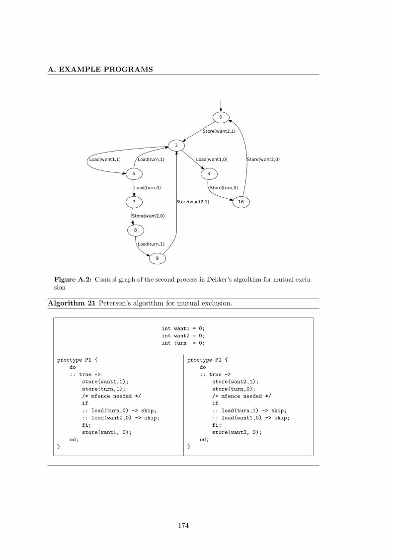
A. EXAMPLE PROGRAMS
0
3
Store(want2,1)
5
Load(want1,1)
4
Load(want1,0)Load(turn,1)
7
Load(turn,0)
16
Store(turn,0)
Store(want2,0)
8
Store(want2,0)
9
Load(turn,1)
Store(want2,1)
Figure A.2: Control graph of the second process in Dekker’s algorithm for mutual exclu-sion
Algorithm 21 Peterson’s algorithm for mutual exclusion.
int want1 = 0;
int want2 = 0;
int turn = 0;
proctype P1
do
:: true ->
store(want1,1);
store(turn,1);
/* mfence needed */
if
:: load(turn,0) -> skip;
:: load(want2,0) -> skip;
fi;
store(want1, 0);
od;
proctype P2
do
:: true ->
store(want2,1);
store(turn,0);
/* mfence needed */
if
:: load(turn,1) -> skip;
:: load(want1,0) -> skip;
fi;
store(want2, 0);
od;
174
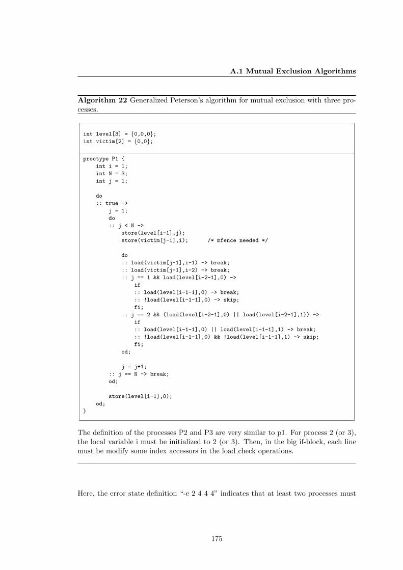
A.1 Mutual Exclusion Algorithms
Algorithm 22 Generalized Peterson’s algorithm for mutual exclusion with three pro-cesses.
int level[3] = 0,0,0;int victim[2] = 0,0;
proctype P1
int i = 1;
int N = 3;
int j = 1;
do
:: true ->
j = 1;
do
:: j < N ->
store(level[i-1],j);
store(victim[j-1],i); /* mfence needed */
do
:: load(victim[j-1],i-1) -> break;
:: load(victim[j-1],i-2) -> break;
:: j == 1 && load(level[i-2-1],0) ->
if
:: load(level[i-1-1],0) -> break;
:: !load(level[i-1-1],0) -> skip;
fi;
:: j == 2 && (load(level[i-2-1],0) || load(level[i-2-1],1)) ->
if
:: load(level[i-1-1],0) || load(level[i-1-1],1) -> break;
:: !load(level[i-1-1],0) && !load(level[i-1-1],1) -> skip;
fi;
od;
j = j+1;
:: j == N -> break;
od;
store(level[i-1],0);
od;
The definition of the processes P2 and P3 are very similar to p1. For process 2 (or 3),the local variable i must be initialized to 2 (or 3). Then, in the big if-block, each linemust be modify some index accessors in the load check operations.
Here, the error state definition “-e 2 4 4 4” indicates that at least two processes must
175
A. EXAMPLE PROGRAMS
locate in their corresponding control location in order to form a “bad state”.
A.1.4 Lamport’s Fast Mutex
Another currently known algorithm is Lamport’s Fast Mutex for N processes designed
to have a bounded number of required memory accesses before entering the critical
section. The algorithm broken down to two processes is given in Algorithm 23.
Safety property preservation for TSO is done by running the tool with the arguments
-f fast mutex.txt -P safety -MM TSO -Mode errorCorrection -e 2 36 36
but which produces a fence set containing useless fences, and thus the fence set can be
shrinked to be maximal permissive by adding the option -maximalPermissive.
A.1.5 Dijkstra
The next mutual exclusion algorithm we consider is Dijkstra’s. The instance of the
algorithm for two processes is shown in Algorithm 24.
The arguments to pass to the tool in order to preserve the safety property are
-f dijkstra.txt -P safety -MM TSO -Mode errorCorrection -e 2 3 3
A.1.6 Burns
Burn’s algorithm for mutual exclusion is given in Algorithm 25.
The arguments to pass to the tool in order to preserve the safety property are
-f burns.txt -P safety -MM TSO -Mode errorCorrection -e 2 4 3
A.1.7 Szymanski
Szymanski’s algorithm for mutual exclusion can also be modified to preserve the safety
property, and is given in Algorithm 26.
The arguments to pass to the tool in order to preserve the safety property are
-f szymanski.txt -P safety -MM TSO -Mode errorCorrection -e 2 16 17
but which produces a fence set containing useless fences, and thus the fence set can be
shrinked by the option -maximalPermissive to remove those useless fences.
176
A.2 TSO/PSO-Safe Programs
A.1.8 Lamport’s Bakery
The last mutual exclusion algorithm we considered consists in Lamport’s Bakery. This
algorithm is not finite-state in SC, and thus we cannot handle the version in which
each process tries entering the critical section repeatedly. However, when bounding the
ticket-numbers, we can do so. Algorithm 27 contains the version we considered where
both processes enter the critical section repeatedly with bounded ticket-number.
The arguments to pass to the tool in order to preserve the safety property are
-f bakery 2 bound.txt -P safety -MM TSO -Mode errorCorrection -e 2 15 15
For this Lamport’s Bakery algorithm, we also considered the instance with 3 pro-
cesses by also bounding the ticket-number to 3, and could successfully infer the fences
and verify safety after this insertion. The program, which has to be more general than
the 2-process version, is given in Algorithm 28.
The arguments to pass to the tool in order to preserve the safety property are
-f bakery 3 bound.txt -P safety -MM TSO -Mode errorCorrection -e 2 28 28 28
A.2 TSO/PSO-Safe Programs
In this section, we provide the example programs where a safety property is satisfied by
the program even when executed on a TSO/PSO memory system. For those programs,
we could successfully compute the state space while no error has been detected.
A.2.1 Alternating Bit Protocol
The first program we considered is the alternating bit protocol. Algorithm 29 gives
the input code for our tool. This version models the alternating bit protocol by two
shared variables (taken from [1]), and where we need to check that no process can start
writing the next message or acknowledgment before the other program has read it.
The arguments to pass to the tool in order to compute the state space with respect
to the safety property are
-f alternating bit.txt -P safety -MM TSO -Mode allErrors -e 2 3 12 -e 2 12 3
where each error state represents the fact that one process already reached the block
where the next message/acknowledgment will be send without the other process having
read the previous message/acknowledgment of the first process.
177
A. EXAMPLE PROGRAMS
A.2.2 CLH Queue Lock
The next TSO/PSO-safe program is the mutual exclusion algorithm CLH queue lock.
The version we considered is also taken from [1], and where we need to check that only
one process can enter into the critical section at a time. The input code for our tool is
given in Algorithm 30.
The arguments to pass to the tool in order to compute the state space with respect
to the safety property are
-f clh queue lock.txt -P safety -MM TSO -Mode allErrors -e 2 15 15
A.2.3 Increasing Sequence
The last example to consider as TSO/PSO-safe programs with respect to safety prop-
erties is the increasing sequence already described earlier. In this program, a server
process (P1) writes an increasing sequence to a shared memory location m, where the
process may write the same value several times, but where the values written to m only
can increase but never decrease and are bounded by 10. A second process (P2) will read
the value from m twice. Then, it is requested that the first read value is lower or equal
to the second value read. The corresponding input program is given in Algorithm 31.
The arguments to pass to the tool in order to compute the state space with respect
to the safety property are
-f increasing sequence.txt -P safety -MM TSO -Mode allErrors -e 1 100 4
A.3 Different Types of Cycles
In this section, we provide some simple example programs with different mixable cycles,
illustrating the acceleration of these.
A.3.1 Mixable Cycles
This first example of cycles has two cycles which are mixable. Then, our tool can
accelerate both cycles and stores the effect of the repeated and mixed execution of the
cycles in the buffer automaton. Algorithm 32 gives the input file for that program.
The arguments to pass to the tool in order to compute the state space with respect
to the safety property (which is not existing in this example, but we need to set some
artificial error state) are
-f parallel cycles1.txt -P safety -MM TSO -Mode stateSpace -e 1 100
178
A.4 Program with Deadlock under TSO/PSO
A.3.2 Mixable Cycles 2
This example has three cycles, all starting and ending in the same control location, but
among which only two are mixable while the third is not mixable with the first two.
Our tool can compute the whole state space by accelerating these cycles. Algorithm 33
shows the input file of that program.
The arguments to pass to the tool in order to compute the state space with respect
to the safety property (which is again not existing in this example) are
-f parallel cycles2.txt -P safety -MM TSO -Mode stateSpace -e 1 100
A.3.3 Cycle Unlocking Example
This section provides an example illustrating a cycle which becomes possible (i.e. which
is unlocked) to accelerate only after a cycle of another process has been accelerated.
Algorithm 34 gives the input code of the program. Here, process P1 can freely loop
from the beginning because the variable y is set to 1 initially. Thus, one can accelerate
the cycle in P1’s control graph. In contrast, process P2 needs the value of x to alternate
between 0 and 1 during its cycle. This cycle can thus not freely loop from the beginning.
However, once P1 has accelerated its cycle, P2 can freely loop by using the buffer
contents of P1’s buffer automaton.
The arguments to pass to the tool in order to compute the state space with respect
to the safety property (which is again not existing in this example) are
-f cycle unlocking.txt -P safety -MM TSO -Mode stateSpace -e 1 100
A.4 Program with Deadlock under TSO/PSO
This section gives an example program having a deadlock when executed under TSO
or PSO, but not under SC. Algorithm 35 gives the input file to our tool of the program.
The arguments to pass to the tool in order to compute the state space with respect
to the absence of deadlocks are
-f deadlock.txt -P deadlock -MM TSO -Mode allErrors
When correcting the program is required, simply change the Mode-Option to become
errorCorrection.
179
A. EXAMPLE PROGRAMS
A.5 TSO-Safe Program Not being PSO-Safe
This section gives an example program which is TSO-safe but not PSO-safe with re-
spect to absence of deadlock. This example illustrates that the acceleration technique
takes well into account sfence buffer symbols representing executed sfence instructions.
Algorithm 36 provides the input file of that program, having two processes. The idea
is that the first process P1 starts with writing an undefined number of times the value
1 to x and to y. Afterwards, P0 writes the value 1 to z. The variables x,y and z are
all set to 0 initially. Then (or before), P2 starts its execution. In a first if-block, it will
read z, which is either 0 or 1. If P2 reads 1 for z, then it will quit the first if-block.
Otherwise, it will check if y has already been set to 1 in the shared memory. If not,
P2 also quits the first if-block after waiting for z to be 1. Otherwise, if y has already
been set to 1, it must load 1 for x, and will block otherwise, which is only possible
under PSO. Then again, P1 can quit the if-block only after reading the value 1 for z.
If P2 can quit the first if-block, than it continues with a second if-block. Note that if
P2 quits this block, z is set to 1. In this second if-block, the values of x and y must be
the same when considering SC or TSO. However, under PSO, it is possible that both
loaded values for x and y differ, and a deadlock is reachable. This can be avoided by
placing an sfence between the two stores to x and y in P0.
The arguments to pass to the tool in order to compute the state space with respect
to deadlocks are
-f sfence.txt -P deadlock -MM TSO -Mode allErrors
while the correction of the errors can be performed by changing the mode option to
errorCorrection.
180
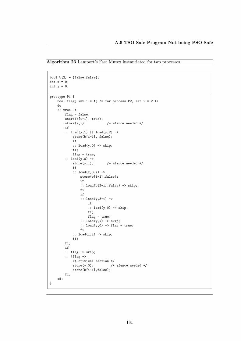
A.5 TSO-Safe Program Not being PSO-Safe
Algorithm 23 Lamport’s Fast Mutex instantiated for two processes.
bool b[2] = false,false;int x = 0;
int y = 0;
proctype P1
bool flag; int i = 1; /* for process P2, set i = 2 */
do
:: true ->
flag = false;
store(b[i-1], true);
store(x,i); /* mfence needed */
if
:: load(y,1) || load(y,2) ->
store(b[i-1], false);
if
:: load(y,0) -> skip;
fi;
flag = true;
:: load(y,0) ->
store(y,i); /* mfence needed */
if
:: load(x,3-i) ->
store(b[i-1],false);
if
:: load(b[2-i],false) -> skip;
fi;
if
:: load(y,3-i) ->
if
:: load(y,0) -> skip;
fi;
flag = true;
:: load(y,i) -> skip;
:: load(y,0) -> flag = true;
fi;
:: load(x,i) -> skip;
fi;
fi;
if
:: flag -> skip;
:: !flag ->
/* critical section */
store(y,0); /* sfence needed */
store(b[i-1],false);
fi;
od;
181
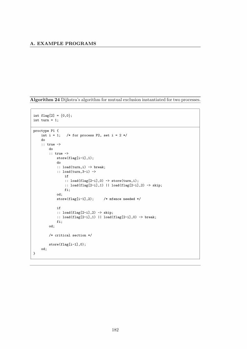
A. EXAMPLE PROGRAMS
Algorithm 24 Dijkstra’s algorithm for mutual exclusion instantiated for two processes.
int flag[2] = 0,0;int turn = 1;
proctype P1
int i = 1; /* for process P2, set i = 2 */
do
:: true ->
do
:: true ->
store(flag[i-1],1);
do
:: load(turn,i) -> break;
:: load(turn,3-i) ->
if
:: load(flag[2-i],0) -> store(turn,i);
:: load(flag[2-i],1) || load(flag[2-i],2) -> skip;
fi;
od;
store(flag[i-1],2); /* mfence needed */
if
:: load(flag[2-i],2) -> skip;
:: load(flag[2-i],1) || load(flag[2-i],0) -> break;
fi;
od;
/* critical section */
store(flag[i-1],0);
od;
182
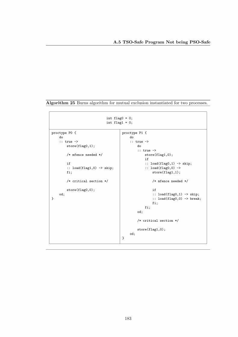
A.5 TSO-Safe Program Not being PSO-Safe
Algorithm 25 Burns algorithm for mutual exclusion instantiated for two processes.
int flag0 = 0;
int flag1 = 0;
proctype P0
do
:: true ->
store(flag0,1);
/* mfence needed */
if
:: load(flag1,0) -> skip;
fi;
/* critical section */
store(flag0,0);
od;
proctype P1
do
:: true ->
do
:: true ->
store(flag1,0);
if
:: load(flag0,1) -> skip;
:: load(flag0,0) ->
store(flag1,1);
/* mfence needed */
if
:: load(flag0,1) -> skip;
:: load(flag0,0) -> break;
fi;
fi;
od;
/* critical section */
store(flag1,0);
od;
183
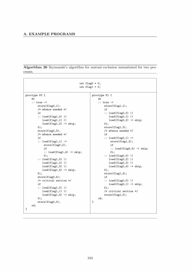
A. EXAMPLE PROGRAMS
Algorithm 26 Szymanski’s algorithm for mutual exclusion instantiated for two pro-cesses.
int flag0 = 0;
int flag1 = 0;
proctype P0
do
:: true ->
store(flag0,1);
/* mfence needed */
if
:: load(flag1,0) ||
load(flag1,1) ||
load(flag1,2) -> skip;
fi;
store(flag0,3);
/* mfence needed */
if
:: load(flag1,1) ->
store(flag0,2);
if
:: load(flag1,4) -> skip;
fi;
:: load(flag1,0) ||
load(flag1,2) ||
load(flag1,3) ||
load(flag1,4) -> skip;
fi;
store(flag0,4);
/* critical section */
if
:: load(flag1,0) ||
load(flag1,1) ||
load(flag1,4) -> skip;
fi;
store(flag0,0);
od;
proctype P1
do
:: true ->
store(flag1,1);
if
:: load(flag0,0) ||
load(flag0,1) ||
load(flag0,2) -> skip;
fi;
store(flag1,3);
/* mfence needed */
if
:: load(flag0,1) ->
store(flag1,2);
if
:: load(flag0,4) -> skip;
fi;
:: load(flag0,0) ||
load(flag0,2) ||
load(flag0,3) ||
load(flag0,4) -> skip;
fi;
store(flag1,4);
if
:: load(flag0,0) ||
load(flag0,1) -> skip;
fi;
/* critical section */
store(flag1,0);
od;
184
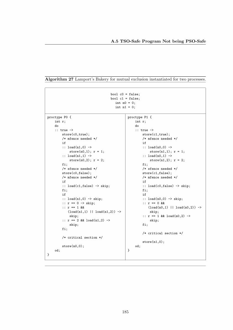
A.5 TSO-Safe Program Not being PSO-Safe
Algorithm 27 Lamport’s Bakery for mutual exclusion instantiated for two processes.
bool c0 = false;
bool c1 = false;
int n0 = 0;
int n1 = 0;
proctype P0
int r;
do
:: true ->
store(c0,true);
/* mfence needed */
if
:: load(n1,0) ->
store(n0,1); r = 1;
:: load(n1,1) ->
store(n0,2); r = 2;
fi;
/* sfence needed */
store(c0,false);
/* mfence needed */
if
:: load(c1,false) -> skip;
fi;
if
:: load(n1,0) -> skip;
:: r == 0 -> skip;
:: r == 1 &&
(load(n1,1) || load(n1,2)) ->
skip;
:: r == 2 && load(n1,2) ->
skip;
fi;
/* critical section */
store(n0,0);
od;
proctype P1
int r;
do
:: true ->
store(c1,true);
/* mfence needed */
if
:: load(n0,0) ->
store(n1,1); r = 1;
:: load(n0,1) ->
store(n1,2); r = 2;
fi;
/* sfence needed */
store(c1,false);
/* mfence needed */
if
:: load(c0,false) -> skip;
fi;
if
:: load(n0,0) -> skip;
:: r == 0 &&
(load(n0,1) || load(n0,2)) ->
skip;
:: r == 1 && load(n0,2) ->
skip;
fi;
/* critical section */
store(n1,0);
od;
185
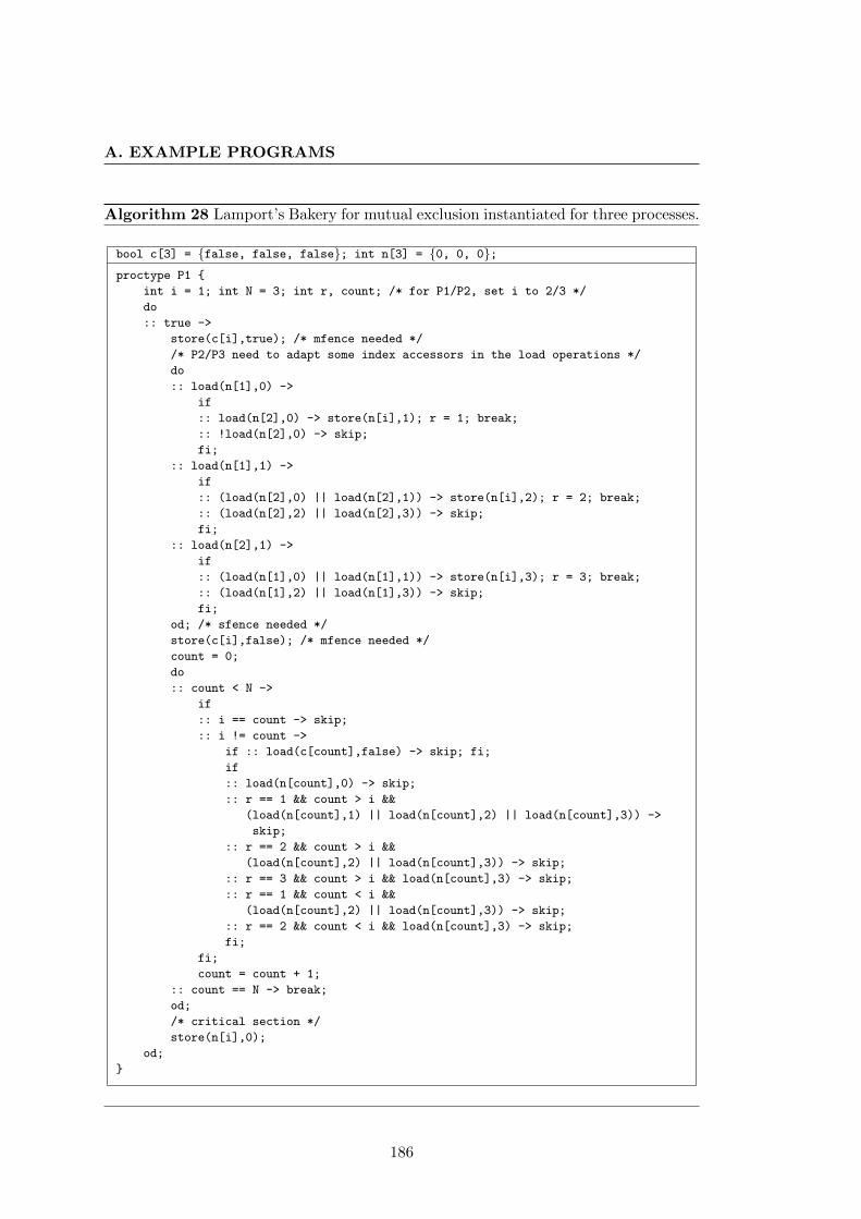
A. EXAMPLE PROGRAMS
Algorithm 28 Lamport’s Bakery for mutual exclusion instantiated for three processes.
bool c[3] = false, false, false; int n[3] = 0, 0, 0;proctype P1
int i = 1; int N = 3; int r, count; /* for P1/P2, set i to 2/3 */
do
:: true ->
store(c[i],true); /* mfence needed */
/* P2/P3 need to adapt some index accessors in the load operations */
do
:: load(n[1],0) ->
if
:: load(n[2],0) -> store(n[i],1); r = 1; break;
:: !load(n[2],0) -> skip;
fi;
:: load(n[1],1) ->
if
:: (load(n[2],0) || load(n[2],1)) -> store(n[i],2); r = 2; break;
:: (load(n[2],2) || load(n[2],3)) -> skip;
fi;
:: load(n[2],1) ->
if
:: (load(n[1],0) || load(n[1],1)) -> store(n[i],3); r = 3; break;
:: (load(n[1],2) || load(n[1],3)) -> skip;
fi;
od; /* sfence needed */
store(c[i],false); /* mfence needed */
count = 0;
do
:: count < N ->
if
:: i == count -> skip;
:: i != count ->
if :: load(c[count],false) -> skip; fi;
if
:: load(n[count],0) -> skip;
:: r == 1 && count > i &&
(load(n[count],1) || load(n[count],2) || load(n[count],3)) ->
skip;
:: r == 2 && count > i &&
(load(n[count],2) || load(n[count],3)) -> skip;
:: r == 3 && count > i && load(n[count],3) -> skip;
:: r == 1 && count < i &&
(load(n[count],2) || load(n[count],3)) -> skip;
:: r == 2 && count < i && load(n[count],3) -> skip;
fi;
fi;
count = count + 1;
:: count == N -> break;
od;
/* critical section */
store(n[i],0);
od;
186
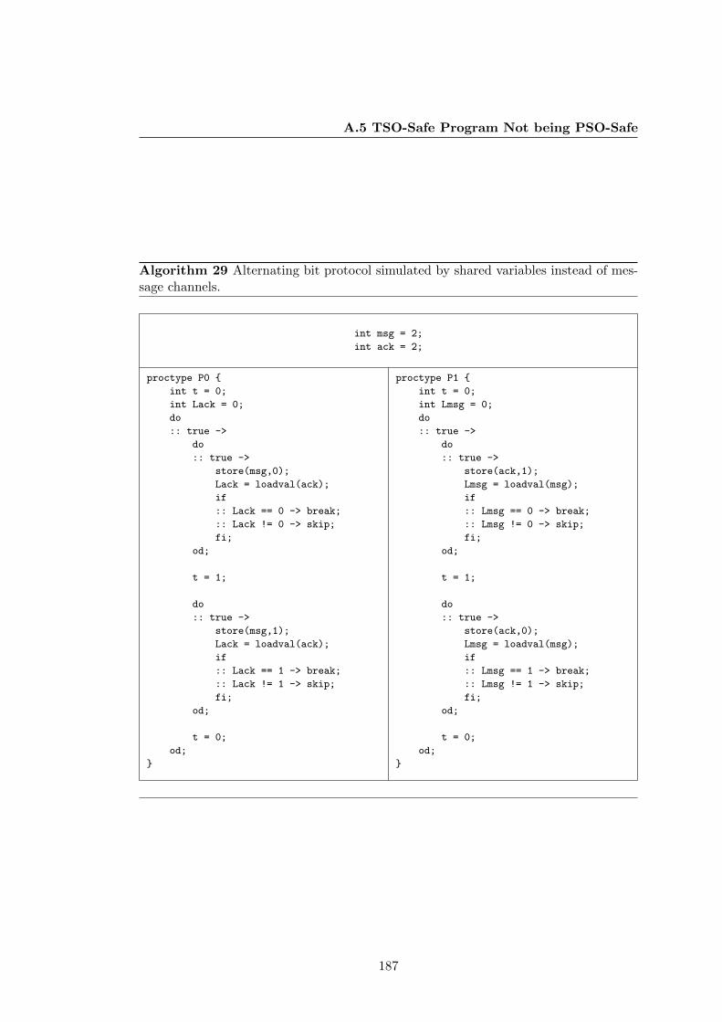
A.5 TSO-Safe Program Not being PSO-Safe
Algorithm 29 Alternating bit protocol simulated by shared variables instead of mes-sage channels.
int msg = 2;
int ack = 2;
proctype P0
int t = 0;
int Lack = 0;
do
:: true ->
do
:: true ->
store(msg,0);
Lack = loadval(ack);
if
:: Lack == 0 -> break;
:: Lack != 0 -> skip;
fi;
od;
t = 1;
do
:: true ->
store(msg,1);
Lack = loadval(ack);
if
:: Lack == 1 -> break;
:: Lack != 1 -> skip;
fi;
od;
t = 0;
od;
proctype P1
int t = 0;
int Lmsg = 0;
do
:: true ->
do
:: true ->
store(ack,1);
Lmsg = loadval(msg);
if
:: Lmsg == 0 -> break;
:: Lmsg != 0 -> skip;
fi;
od;
t = 1;
do
:: true ->
store(ack,0);
Lmsg = loadval(msg);
if
:: Lmsg == 1 -> break;
:: Lmsg != 1 -> skip;
fi;
od;
t = 0;
od;
187
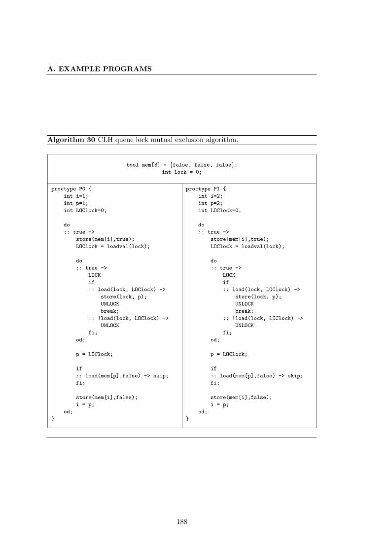
A. EXAMPLE PROGRAMS
Algorithm 30 CLH queue lock mutual exclusion algorithm.
bool mem[3] = false, false, false;int lock = 0;
proctype P0
int i=1;
int p=1;
int LOClock=0;
do
:: true ->
store(mem[i],true);
LOClock = loadval(lock);
do
:: true ->
LOCK
if
:: load(lock, LOClock) ->
store(lock, p);
UNLOCK
break;
:: !load(lock, LOClock) ->
UNLOCK
fi;
od;
p = LOClock;
if
:: load(mem[p],false) -> skip;
fi;
store(mem[i],false);
i = p;
od;
proctype P1
int i=2;
int p=2;
int LOClock=0;
do
:: true ->
store(mem[i],true);
LOClock = loadval(lock);
do
:: true ->
LOCK
if
:: load(lock, LOClock) ->
store(lock, p);
UNLOCK
break;
:: !load(lock, LOClock) ->
UNLOCK
fi;
od;
p = LOClock;
if
:: load(mem[p],false) -> skip;
fi;
store(mem[i],false);
i = p;
od;
188
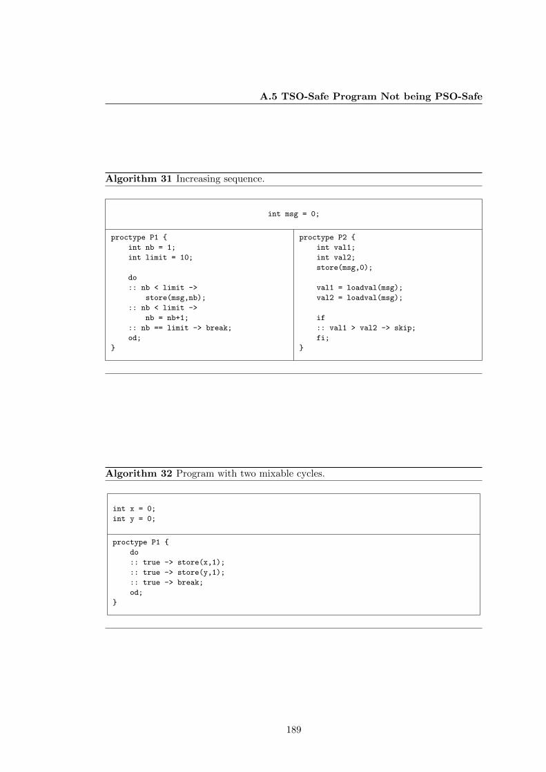
A.5 TSO-Safe Program Not being PSO-Safe
Algorithm 31 Increasing sequence.
int msg = 0;
proctype P1
int nb = 1;
int limit = 10;
do
:: nb < limit ->
store(msg,nb);
:: nb < limit ->
nb = nb+1;
:: nb == limit -> break;
od;
proctype P2
int val1;
int val2;
store(msg,0);
val1 = loadval(msg);
val2 = loadval(msg);
if
:: val1 > val2 -> skip;
fi;
Algorithm 32 Program with two mixable cycles.
int x = 0;
int y = 0;
proctype P1
do
:: true -> store(x,1);
:: true -> store(y,1);
:: true -> break;
od;
189
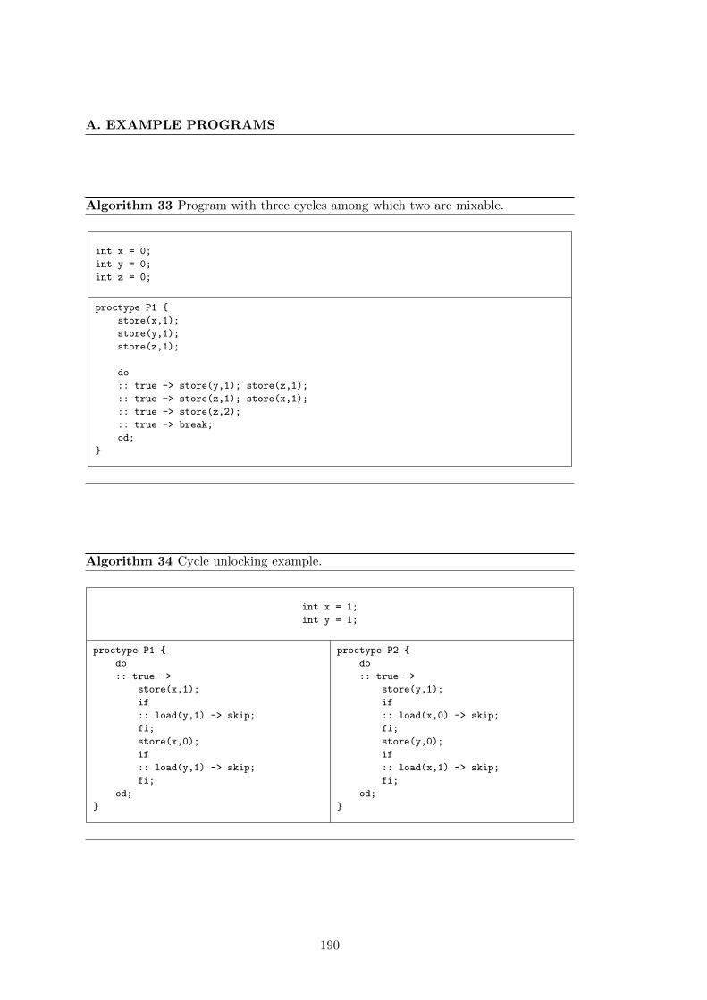
A. EXAMPLE PROGRAMS
Algorithm 33 Program with three cycles among which two are mixable.
int x = 0;
int y = 0;
int z = 0;
proctype P1
store(x,1);
store(y,1);
store(z,1);
do
:: true -> store(y,1); store(z,1);
:: true -> store(z,1); store(x,1);
:: true -> store(z,2);
:: true -> break;
od;
Algorithm 34 Cycle unlocking example.
int x = 1;
int y = 1;
proctype P1
do
:: true ->
store(x,1);
if
:: load(y,1) -> skip;
fi;
store(x,0);
if
:: load(y,1) -> skip;
fi;
od;
proctype P2
do
:: true ->
store(y,1);
if
:: load(x,0) -> skip;
fi;
store(y,0);
if
:: load(x,1) -> skip;
fi;
od;
190
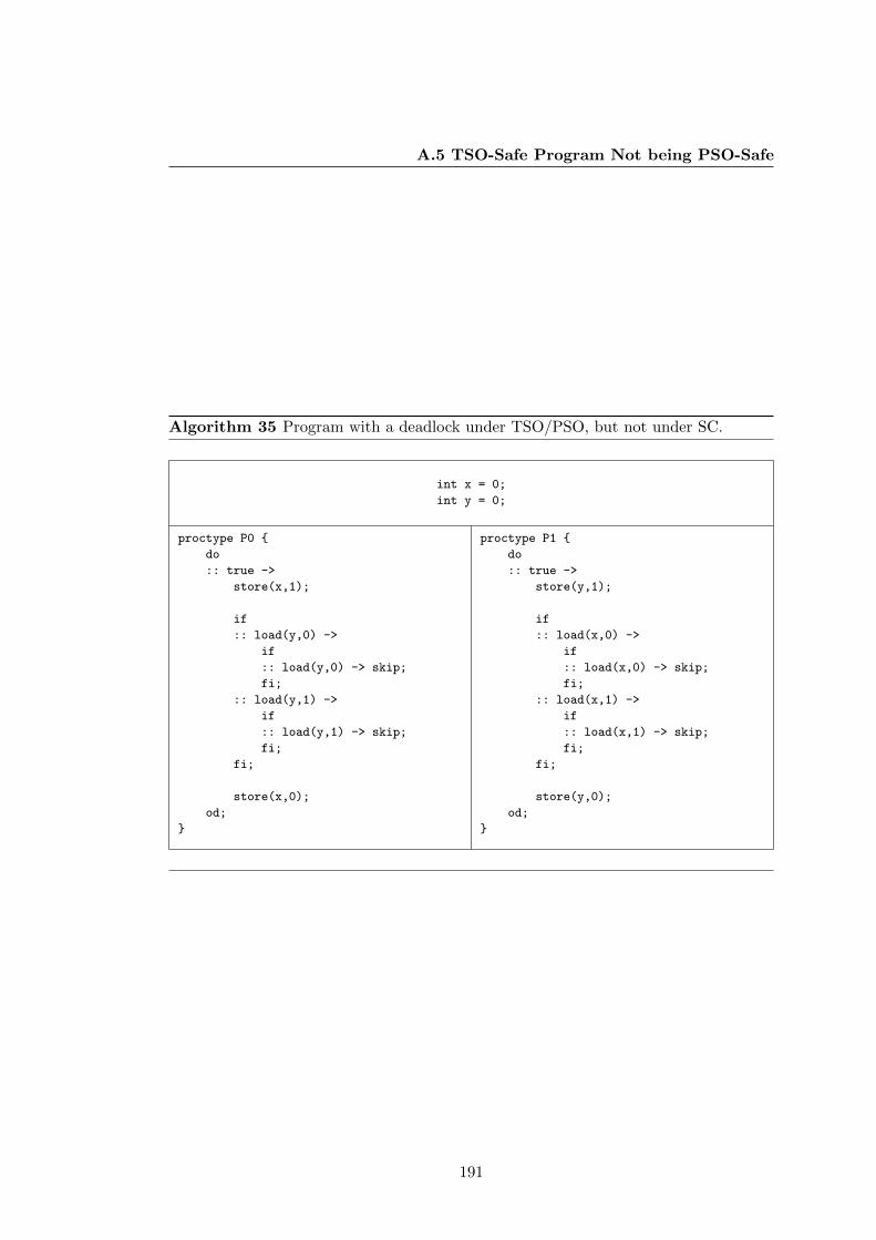
A.5 TSO-Safe Program Not being PSO-Safe
Algorithm 35 Program with a deadlock under TSO/PSO, but not under SC.
int x = 0;
int y = 0;
proctype P0
do
:: true ->
store(x,1);
if
:: load(y,0) ->
if
:: load(y,0) -> skip;
fi;
:: load(y,1) ->
if
:: load(y,1) -> skip;
fi;
fi;
store(x,0);
od;
proctype P1
do
:: true ->
store(y,1);
if
:: load(x,0) ->
if
:: load(x,0) -> skip;
fi;
:: load(x,1) ->
if
:: load(x,1) -> skip;
fi;
fi;
store(y,0);
od;
191
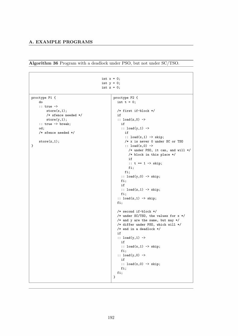
A. EXAMPLE PROGRAMS
Algorithm 36 Program with a deadlock under PSO, but not under SC/TSO.
int x = 0;
int y = 0;
int z = 0;
proctype P1
do
:: true ->
store(x,1);
/* sfence needed */
store(y,1);
:: true -> break;
od;
/* sfence needed */
store(z,1);
proctype P2
int t = 0;
/* first if-block */
if
:: load(z,0) ->
if
:: load(y,1) ->
if
:: load(x,1) -> skip;
/* x is never 0 under SC or TSO
:: load(x,0) ->
/* under PSO, it can, and will */
/* block in this place */
if
:: t == 1 -> skip;
fi;
fi;
:: load(y,0) -> skip;
fi;
if
:: load(z,1) -> skip;
fi;
:: load(z,1) -> skip;
fi;
/* second if-block */
/* under SC/TSO, the values for x */
/* and y are the same, but may */
/* differ under PSO, which will */
/* end in a deadlock */
if
:: load(y,1) ->
if
:: load(x,1) -> skip;
fi;
:: load(y,0) ->
if
:: load(x,0) -> skip;
fi;
fi;
192
Bibliography
[1] Abdulla, P. A., Atig, M. F., Chen, Y.-F., Leonardsson, C., and Rezine,
A. Counter-Example guided fence insertion under TSO. In Proceedings of the 18th
international conference on Tools and Algorithms for the Construction and Anal-
ysis of Systems (Berlin, Heidelberg, 2012), TACAS’12, Springer-Verlag, pp. 204–
219.
[2] Abdulla, P. A., Atig, M. F., Chen, Y.-F., Leonardsson, C., and Rezine,
A. MEMORAX, a precise and sound tool for automatic fence insertion under TSO.
In Proceedings of the 19th international conference on Tools and Algorithms for
the Construction and Analysis of Systems (Berlin, Heidelberg, 2013), TACAS’13,
Springer-Verlag, pp. 530–536.
[3] Abdulla, P. A., Bouajjani, A., and Jonsson, B. On-the-Fly Analysis of
Systems with Unbounded, Lossy FIFO Channels. In Proceedings of the 10th In-
ternational Conference on Computer Aided Verification (London, UK, UK, 1998),
CAV ’98, Springer-Verlag, pp. 305–318.
[4] Abdulla, P. A., Collomb-Annichini, A., Bouajjani, A., and Jonsson, B.
Using Forward Reachability Analysis for Verification of Lossy Channel Systems.
Form. Methods Syst. Des. 25, 1 (July 2004), 39–65.
[5] Abdulla, P. A., and Jonsson, B. Undecidable Verification Problems for Pro-
grams with Unreliable Channels. Information and Computation 130, 1 (Oct. 1996),
71–90.
[6] Abdulla, P. A., and Jonsson, B. Verifying Programs with Unreliable Chan-
nels. Information and Computation 127, 2 (1996), 91 – 101.
[7] Abdulla, P. A., Kindahl, M., and Peled, D. An Improved Search Strategy
for Lossy Channel Systems. In Proceedings of the IFIP TC6 WG6.1 Joint In-
ternational Conference on Formal Description Techniques for Distributed Systems
193
BIBLIOGRAPHY
and Communication Protocols (FORTE X) and Protocol Specification, Testing and
Verification (PSTV XVII) (London, UK, UK, 1998), FORTE X / PSTV XVII ’97,
Chapman & Hall, Ltd., pp. 251–264.
[8] Alglave, J., Kroening, D., Nimal, V., and Tautschnig, M. Software veri-
fication for weak memory via program transformation. In Proceedings of the 22nd
European conference on Programming Languages and Systems (Berlin, Heidelberg,
2013), ESOP’13, Springer-Verlag, pp. 512–532.
[9] Alglave, J., and Maranget, L. Stability in weak memory models. In Proceed-
ings of the 23rd international conference on Computer aided verification (Berlin,
Heidelberg, 2011), CAV’11, Springer-Verlag, pp. 50–66.
[10] Alglave, J., Maranget, L., Sarkar, S., and Sewell, P. Fences in weak
memory models (extended version). Form. Methods Syst. Des. 40, 2 (Apr. 2012),
170–205.
[11] Atig, M. F., Bouajjani, A., Burckhardt, S., and Musuvathi, M. On
the verification problem for weak memory models. In Proceedings of the 37th
annual ACM SIGPLAN-SIGACT symposium on Principles of programming lan-
guages (New York, NY, USA, 2010), POPL ’10, ACM, pp. 7–18.
[12] Atig, M. F., Bouajjani, A., Burckhardt, S., and Musuvathi, M. What’s
decidable about weak memory models? In Proceedings of the 21st European
conference on Programming Languages and Systems (Berlin, Heidelberg, 2012),
ESOP’12, Springer-Verlag, pp. 26–46.
[13] Atig, M. F., Bouajjani, A., and Parlato, G. Getting rid of store-buffers in
TSO analysis. In Proceedings of the 23rd international conference on Computer
aided verification (Berlin, Heidelberg, 2011), CAV’11, Springer-Verlag, pp. 99–115.
[14] Attiya, H., Guerraoui, R., Hendler, D., Kuznetsov, P., Michael,
M. M., and Vechev, M. Laws of Order: Expensive Synchronization in Concur-
rent Algorithms cannot be Eliminated. In Proceedings of the 38th annual ACM
SIGPLAN-SIGACT symposium on Principles of programming languages (New
York, NY, USA, 2011), POPL ’11, ACM, pp. 487–498.
[15] Boigelot, B. Symbolic Methods for Exploring Infinite State Spaces. PhD thesis,
Universite de Liege, 1999.
194
BIBLIOGRAPHY
[16] Boigelot, B., and Godefroid, P. Symbolic Verification of Communication
Protocols with Infinite State Spaces Using QDDs (Extended Abstract). In Proceed-
ings of the 8th International Conference on Computer Aided Verification (London,
UK, UK, 1996), CAV ’96, Springer-Verlag, pp. 1–12.
[17] Boigelot, B., and Godefroid, P. Symbolic Verification of Communication
Protocols with Infinite State Spaces using QDDs. Form. Methods Syst. Des. 14, 3
(May 1999), 237–255.
[18] Boigelot, B., Godefroid, P., Willems, B., and Wolper, P. The Power of
QDDs (Extended Abstract). In Proceedings of the 4th International Symposium on
Static Analysis (London, UK, UK, 1997), SAS ’97, Springer-Verlag, pp. 172–186.
[19] Boigelot, B., and Wolper, P. Symbolic Verification with Periodic Sets. In
Proceedings of the 6th International Conference on Computer Aided Verification
(London, UK, UK, 1994), CAV ’94, Springer-Verlag, pp. 55–67.
[20] Bouajjani, A., Derevenetc, E., and Meyer, R. Checking and enforcing
robustness against TSO. In Proceedings of the 22nd European conference on Pro-
gramming Languages and Systems (Berlin, Heidelberg, 2013), ESOP’13, Springer-
Verlag, pp. 533–553.
[21] Bouajjani, A., Meyer, R., and Mohlmann, E. Deciding robustness against
total store ordering. In Proceedings of the 38th international conference on Au-
tomata, languages and programming - Volume Part II (Berlin, Heidelberg, 2011),
ICALP’11, Springer-Verlag, pp. 428–440.
[22] Burckhardt, S., Alur, R., and Martin, M. M. K. Checkfence: checking
consistency of concurrent data types on relaxed memory models. SIGPLAN Not.
42, 6 (June 2007), 12–21.
[23] Burckhardt, S., and Musuvathi, M. Effective Program Verification for Re-
laxed Memory Models. In Proceedings of the 20th international conference on
Computer Aided Verification (Berlin, Heidelberg, 2008), CAV ’08, Springer-Verlag,
pp. 107–120.
[24] Burnim, J., Sen, K., and Stergiou, C. Sound and complete monitoring of
sequential consistency for relaxed memory models. In Proceedings of the 17th in-
ternational conference on Tools and algorithms for the construction and analysis of
systems: part of the joint European conferences on theory and practice of software
(Berlin, Heidelberg, 2011), TACAS’11/ETAPS’11, Springer-Verlag, pp. 11–25.
195
BIBLIOGRAPHY
[25] Cece, G., Finkel, A., and Iyer, S. P. Unreliable channels are easier to verify
than perfect channels. Information and Computation 124, 1 (Jan. 1996), 20–31.
[26] Clarke, Jr., E. M., Grumberg, O., and Peled, D. A. Model checking. MIT
Press, Cambridge, MA, USA, 1999.
[27] Dan, A. M., Meshman, Y., Vechev, M. T., and Yahav, E. Predicate Ab-
straction for Relaxed Memory Models. In Proceedings of Static Analysis - 20th
International Symposium (2013), SAS ’13, pp. 84–104.
[28] Dijkstra, E. W. The origin of concurrent programming. Springer-Verlag New
York, Inc., New York, NY, USA, 2002, ch. Cooperating sequential processes,
pp. 65–138.
[29] Fang, X., Lee, J., and Midkiff, S. P. Automatic Fence Insertion for Shared
Memory Multiprocessing. In Proceedings of the 17th annual international confer-
ence on Supercomputing (New York, NY, USA, 2003), ICS ’03, ACM, pp. 285–294.
[30] Godefroid, P. Using Partial Orders to Improve Automatic Verification Methods.
In Proceedings of the 2nd International Workshop on Computer Aided Verification
(London, UK, UK, 1991), CAV ’90, Springer-Verlag, pp. 176–185.
[31] Godefroid, P. Partial-Order Methods for the Verification of Concurrent Sys-
tems: An Approach to the State-Explosion Problem. Springer-Verlag New York,
Inc., Secaucus, NJ, USA, 1996.
[32] Godefroid, P., and Pirottin, D. Refining Dependencies Improves Partial-
Order Verification Methods (Extended Abstract). In Proceedings of the 5th Inter-
national Conference on Computer Aided Verification (London, UK, 1993), CAV
’93, Springer-Verlag, pp. 438–449.
[33] Hangal, S., Vahia, D., Manovit, C., and Lu, J.-Y. J. TSOtool: A Pro-
gram for Verifying Memory Systems Using the Memory Consistency Model. In
Proceedings of the 31st annual international symposium on Computer architecture
(Washington, DC, USA, 2004), ISCA ’04, IEEE Computer Society, pp. 114–.
[34] Holzmann, G. Spin model checker, the: primer and reference manual, first ed.
Addison-Wesley Professional, 2003.
[35] Huynh, T. Q., and Roychoudhury, A. A memory model sensitive checker
for c#. In Proceedings of the 14th international conference on Formal Methods
(Berlin, Heidelberg, 2006), FM’06, Springer-Verlag, pp. 476–491.
196
BIBLIOGRAPHY
[36] Huynh, T. Q., and Roychoudhury, A. Memory model sensitive bytecode
verification. Form. Methods Syst. Des. 31 (December 2007), 281–305.
[37] Intel. Intel® 64 Architecture Memory Ordering White Paper, 2007. SKU 318147-
001.
[38] Intel Corporation. Intel® 64 and IA-32 Architectures Software Developer’s
Manual, vol. 3A. Intel Corporation, March 2010.
[39] Jonsson, B. State-space exploration for concurrent algorithms under weak mem-
ory orderings: (preliminary version). SIGARCH Comput. Archit. News 36 (June
2009), 65–71.
[40] Kuperstein, M., Vechev, M., and Yahav, E. Automatic Inference of Memory
Fences. In Proceedings of the 2010 Conference on Formal Methods in Computer-
Aided Design (Austin, TX, 2010), FMCAD ’10, FMCAD Inc, pp. 111–120.
[41] Kuperstein, M., Vechev, M., and Yahav, E. Partial-Coherence Abstractions
for Relaxed Memory Models. In Proceedings of the 32nd ACM SIGPLAN confer-
ence on Programming language design and implementation (New York, NY, USA,
2011), PLDI ’11, ACM, pp. 187–198.
[42] Lamport, L. A new solution of Dijkstra’s concurrent programming problem.
Commun. ACM 17, 8 (Aug. 1974), 453–455.
[43] Lamport, L. How to Make a Multiprocessor Computer That Correctly Executes
Multiprocess Programs. IEEE Trans. Comput. 28, 9 (Sept. 1979), 690–691.
[44] Lamport, L. A fast mutual exclusion algorithm. ACM Trans. Comput. Syst. 5,
1 (Jan. 1987), 1–11.
[45] Linden, A., and Wolper, P. An Automata-Based Symbolic Approach for
Verifying Programs on Relaxed Memory Models. In Proceedings of the 17th inter-
national SPIN conference on Model checking software (Berlin, Heidelberg, 2010),
SPIN’10, Springer-Verlag, pp. 212–226.
[46] Linden, A., and Wolper, P. A Verification-Based Approach to Memory Fence
Insertion in Relaxed Remory Systems. In Proceedings of the 18th international
SPIN conference on Model checking software (Berlin, Heidelberg, 2011), Springer-
Verlag, pp. 144–160.
197
BIBLIOGRAPHY
[47] Linden, A., and Wolper, P. A Verification-Based Approach to Memory Fence
Insertion in PSO Memory Systems. In Proceedings of the 19th international con-
ference on Tools and Algorithms for the Construction and Analysis of Systems
(Berlin, Heidelberg, 2013), TACAS’13, Springer-Verlag, pp. 339–353.
[48] Liu, F., Nedev, N., Prisadnikov, N., Vechev, M., and Yahav, E. Dynamic
synthesis for relaxed memory models. In Proceedings of the 33rd ACM SIGPLAN
conference on Programming Language Design and Implementation (New York, NY,
USA, 2012), PLDI ’12, ACM, pp. 429–440.
[49] Loewenstein, P., Chaudhry, S., Cypher, R., and Manovit, C. Multipro-
cessor Memory Model Verification.
[50] Lynch, N., and Patt-Shamir, B. Distributed Algorithms, Lecture Notes for
6.852 FALL 1992. Tech. rep., Cambridge, MA, USA, 1993.
[51] Mador-Haim, S., Alur, R., and Martin, M. Generating Litmus Tests for
Contrasting Memory Consistency Models - Extended version. Technical report,
Dept. of Computer Information Science, U. of Pennsylvania, 2010. MS-CIS-10-15.
[52] Mador-Haim, S., Alur, R., and Martin, M. M. Plug and Play Components
for the Exploration of Memory Consistency Models. Tech. rep., University of
Pennsylvania, 2010.
[53] Mador-Haim, S., Alur, R., and Martin, M. M. K. Generating litmus tests
for contrasting memory consistency models. In Proceedings of the 22nd inter-
national conference on Computer Aided Verification (Berlin, Heidelberg, 2010),
CAV’10, Springer-Verlag, pp. 273–287.
[54] Mador-Haim, S., Alur, R., and Martin, M. M. K. Litmus tests for compar-
ing memory consistency models: how long do they need to be? In Proceedings of
the 48th Design Automation Conference (New York, NY, USA, 2011), DAC ’11,
ACM, pp. 504–509.
[55] Mador-Haim, S., Maranget, L., Sarkar, S., Memarian, K., Alglave, J.,
Owens, S., Alur, R., Martin, M. M. K., Sewell, P., and Williams, D.
An axiomatic memory model for POWER multiprocessors. In Proceedings of the
24th international conference on Computer Aided Verification (Berlin, Heidelberg,
2012), CAV’12, Springer-Verlag, pp. 495–512.
198
BIBLIOGRAPHY
[56] Magnusson, P. S., Landin, A., and Hagersten, E. Queue Locks on Cache
Coherent Multiprocessors. In Proceedings of the 8th International Symposium
on Parallel Processing (Washington, DC, USA, 1994), IEEE Computer Society,
pp. 165–171.
[57] Michael, M. M., and Scott, M. L. Simple, fast, and practical non-blocking
and blocking concurrent queue algorithms. In Proceedings of the fifteenth annual
ACM symposium on Principles of distributed computing (New York, NY, USA,
1996), PODC ’96, ACM, pp. 267–275.
[58] Møller, A. dk.brics.automaton – finite-state automata and regular expressions
for Java, 2010. http://www.brics.dk/automaton/.
[59] Owens, S. Reasoning about the implementation of concurrency abstractions on
x86-TSO. In Proceedings of the 24th European conference on Object-oriented pro-
gramming (Berlin, Heidelberg, 2010), ECOOP’10, Springer-Verlag, pp. 478–503.
[60] Owens, S., Sarkar, S., and Sewell, P. A better x86 memory model: x86-
TSO. In Proceedings of the 22nd International Conference on Theorem Proving
in Higher Order Logics (Berlin, Heidelberg, 2009), TPHOLs ’09, Springer-Verlag,
pp. 391–407.
[61] Park, S., and Dill, D. L. An executable specification, analyzer and verifier
for RMO (relaxed memory order). In Proceedings of the seventh annual ACM
symposium on Parallel algorithms and architectures (New York, NY, USA, 1995),
SPAA ’95, ACM, pp. 34–41.
[62] Peled, D. All from One, One for all: on Model Checking Using Representatives.
In Proceedings of the 5th International Conference on Computer Aided Verification
(London, UK, UK, 1993), CAV ’93, Springer-Verlag, pp. 409–423.
[63] Peterson, G. L. Myths About the Mutual Exclusion Problem. Inf. Process.
Lett. 12, 3 (1981), 115–116.
[64] Qadeer, S. Verifying Sequential Consistency on Shared-Memory Multiprocessors
by Model Checking. IEEE Trans. Parallel Distrib. Syst. 14, 8 (Aug. 2003), 730–
741.
[65] Sewell, P., Sarkar, S., Owens, S., Nardelli, F. Z., and Myreen, M. O.
x86-TSO: A Rigorous and Usable Programmer’s Model for x86 Multiprocessors.
Commun. ACM 53 (July 2010), 89–97.
199
BIBLIOGRAPHY
[66] Shasha, D., and Snir, M. Efficient and correct execution of parallel programs
that share memory. ACM Trans. Program. Lang. Syst. 10, 2 (Apr. 1988), 282–312.
[67] Sites, R. L., Ed. Alpha architecture reference manual. Digital Press, Newton,
MA, USA, 1992.
[68] SPARC International, Inc., C. The SPARC architecture manual: version 8.
Prentice-Hall, Inc., Upper Saddle River, NJ, USA, 1992.
[69] SPARC International, Inc., C. The SPARC architecture manual (version 9).
Prentice-Hall, Inc., Upper Saddle River, NJ, USA, 1994.
[70] Szymanski, B. K. A simple solution to Lamport’s concurrent programming prob-
lem with linear wait. In Proceedings of the 2nd international conference on Super-
computing (New York, NY, USA, 1988), ICS ’88, ACM, pp. 621–626.
[71] Valmari, A. Stubborn sets for reduced state space generation. In Proceedings
of the 10th International Conference on Applications and Theory of Petri Nets:
Advances in Petri Nets 1990 (London, UK, 1991), Springer-Verlag, pp. 491–515.
[72] Wolper, P., and Boigelot, B. Verifying Systems with Infinite but Regular
State Spaces. In Proceedings of the 10th International Conference on Computer
Aided Verification (London, UK, UK, 1998), CAV ’98, Springer-Verlag, pp. 88–97.
200
Related Documents