ITS TECHNICAL REPORT NO. 23/2004 1 On the Use of A Priori Information for Sparse Signal Approximations Oscar Divorra Escoda, Lorenzo Granai and Pierre Vandergheynst Signal Processing Institute (ITS) Ecole Polytechnique F´ ed´ erale de Lausanne (EPFL) LTS2-ITS-STI-EPFL, 1015 Lausanne, Switzerland Technical Report No. 23/2004 Abstract This report is the extension to the case of sparse approximations of our previous study on the effects of introducing a priori knowledge to solve the recovery of sparse representations when overcomplete dictionaries are used [1]. Greedy algorithms and Basis Pursuit Denoising are considered in this work. Theoretical results show how the use of “reliable” a priori information (which in this work appears under the form of weights) can improve the performances of these methods. In particular, we generalize the sufficient conditions established by Tropp [2], [3] and Gribonval and Van- dergheynst [4], that guarantee the retrieval of the sparsest solution, to the case where a priori information is used. We prove how the use of prior models at the signal decomposition stage influences these sufficient conditions. The results found in this work reduce to the classical case of [4] and [3] when no a priori information about the signal is available. Finally, examples validate and illustrate theoretical results. Index Terms Sparse Approximations, Sparse Representations, Basis Pursuit Denoising, Matching Pursuit, Relaxation Algo- rithms, Greedy Algorithms, A Priori Knowledge, Redundant Dictionaries, Weighted Basis Pursuit Denoising, Weighted Matching Pursuit. Contents I Introduction 2 II Recovery of General Signals: Sparse Approximations 2 II-A Greedy Algorithms: Weak -MP ...................................... 3 II-A.1 Robustness ........................................... 3 II-A.2 Rate of Convergence ...................................... 4 II-B Convex Relaxation of the Subset Selection Problem .......................... 4 III Including A Priori Information on Greedy algorithms 5 III-A Influence on Sparse Approximations ................................... 5 III-B Rate of Convergence of Weighted-MP/OMP on Sparse Approximations ............... 8 III-C Example: Use of Footprints for -Sparse Approximations........................ 12 IV Approximations with Weighted Basis Pursuit Denoising 13 IV-A A Bayesian Approach to Weighted Basis Pursuit Denoising ...................... 14 IV-B Preliminary Propositions ......................................... 15 IV-C Weighted Relaxed Subset Selection ................................... 17 IV-D Relation with the Weighted Cumulative Coherence .......................... 18 IV-E Example .................................................. 19 V Examples: A Natural Signal Approximation with Coherent Dictionaries and an A Priori Model 19 V-A A Noisy Piecewise-smooth Natural Signal ................................ 20 V-B Modeling the Relation Signal-Dictionary ................................ 21 V-C Signal Approximation ........................................... 21 V-D Results ................................................... 21 V-D.1 Approximation Results with OMP .............................. 21 Web page: http://lts2www.epfl.ch The work of Oscar Divorra Escoda is partly sponsored by the IM.2 NCCR The work of Lorenzo Granai is supported by the SNF grant 2100-066912.01/1

Welcome message from author
This document is posted to help you gain knowledge. Please leave a comment to let me know what you think about it! Share it to your friends and learn new things together.
Transcript
ITS TECHNICAL REPORT NO. 23/2004 1
On the Use of A Priori Information for Sparse
Signal ApproximationsOscar Divorra Escoda, Lorenzo Granai and Pierre Vandergheynst
Signal Processing Institute (ITS)Ecole Polytechnique Federale de Lausanne (EPFL)LTS2-ITS-STI-EPFL, 1015 Lausanne, Switzerland
Technical Report No. 23/2004
Abstract
This report is the extension to the case of sparse approximations of our previous study on the effects of introducinga priori knowledge to solve the recovery of sparse representations when overcomplete dictionaries are used [1]. Greedyalgorithms and Basis Pursuit Denoising are considered in this work. Theoretical results show how the use of “reliable”a priori information (which in this work appears under the form of weights) can improve the performances of thesemethods. In particular, we generalize the sufficient conditions established by Tropp [2], [3] and Gribonval and Van-dergheynst [4], that guarantee the retrieval of the sparsest solution, to the case where a priori information is used. Weprove how the use of prior models at the signal decomposition stage influences these sufficient conditions. The resultsfound in this work reduce to the classical case of [4] and [3] when no a priori information about the signal is available.Finally, examples validate and illustrate theoretical results.
Index Terms
Sparse Approximations, Sparse Representations, Basis Pursuit Denoising, Matching Pursuit, Relaxation Algo-rithms, Greedy Algorithms, A Priori Knowledge, Redundant Dictionaries, Weighted Basis Pursuit Denoising, WeightedMatching Pursuit.
Contents
I Introduction 2
II Recovery of General Signals: Sparse Approximations 2II-A Greedy Algorithms: Weak -MP . . . . . . . . . . . . . . . . . . . . . . . . . . . . . . . . . . . . . . 3
II-A.1 Robustness . . . . . . . . . . . . . . . . . . . . . . . . . . . . . . . . . . . . . . . . . . . 3II-A.2 Rate of Convergence . . . . . . . . . . . . . . . . . . . . . . . . . . . . . . . . . . . . . . 4
II-B Convex Relaxation of the Subset Selection Problem . . . . . . . . . . . . . . . . . . . . . . . . . . 4
III Including A Priori Information on Greedy algorithms 5III-A Influence on Sparse Approximations . . . . . . . . . . . . . . . . . . . . . . . . . . . . . . . . . . . 5III-B Rate of Convergence of Weighted-MP/OMP on Sparse Approximations . . . . . . . . . . . . . . . 8III-C Example: Use of Footprints for ε-Sparse Approximations. . . . . . . . . . . . . . . . . . . . . . . . 12
IV Approximations with Weighted Basis Pursuit Denoising 13IV-A A Bayesian Approach to Weighted Basis Pursuit Denoising . . . . . . . . . . . . . . . . . . . . . . 14IV-B Preliminary Propositions . . . . . . . . . . . . . . . . . . . . . . . . . . . . . . . . . . . . . . . . . 15IV-C Weighted Relaxed Subset Selection . . . . . . . . . . . . . . . . . . . . . . . . . . . . . . . . . . . 17IV-D Relation with the Weighted Cumulative Coherence . . . . . . . . . . . . . . . . . . . . . . . . . . 18IV-E Example . . . . . . . . . . . . . . . . . . . . . . . . . . . . . . . . . . . . . . . . . . . . . . . . . . 19
V Examples: A Natural Signal Approximation with Coherent Dictionaries and an A Priori Model 19V-A A Noisy Piecewise-smooth Natural Signal . . . . . . . . . . . . . . . . . . . . . . . . . . . . . . . . 20V-B Modeling the Relation Signal-Dictionary . . . . . . . . . . . . . . . . . . . . . . . . . . . . . . . . 21V-C Signal Approximation . . . . . . . . . . . . . . . . . . . . . . . . . . . . . . . . . . . . . . . . . . . 21V-D Results . . . . . . . . . . . . . . . . . . . . . . . . . . . . . . . . . . . . . . . . . . . . . . . . . . . 21
V-D.1 Approximation Results with OMP . . . . . . . . . . . . . . . . . . . . . . . . . . . . . . 21
Web page: http://lts2www.epfl.chThe work of Oscar Divorra Escoda is partly sponsored by the IM.2 NCCRThe work of Lorenzo Granai is supported by the SNF grant 2100-066912.01/1
2 ITS TECHNICAL REPORT NO. 23/2004
V-D.2 Approximation Results with BPDN . . . . . . . . . . . . . . . . . . . . . . . . . . . . . 21V-D.3 Capturing the Piecewise-smooth Component with Footprints Basis . . . . . . . . . . . . 23V-D.4 Parameter Search . . . . . . . . . . . . . . . . . . . . . . . . . . . . . . . . . . . . . . . 23
VI Conclusions 24
References 26
I. Introduction
In many applications, such as compression, denoising or source separation, one seeks an efficient representation orapproximation of the signal by means of a linear expansion into a possibly overcomplete family of functions. In thissetting, efficiency is often characterized by sparseness of the associated series of coefficients. The criterion of sparsenesshas been studied for a long time and in the last few years has become popular in the signal processing community [5],[6], [2], [3]. Natural signals are very unlikely to be exact sparse superpositions of vectors. In fact the set of such signalsis of measure zero in C
N [2]. We thus extend our previous work on sparse exact representations [1] to the more usefulcase of sparse approximations:
minc
‖f − Dc‖22 s.t. ‖c‖0 ≤ m. (1)
In general, the problem of recovering the sparsest signal approximation (or representation) over a redundant dictio-nary is a NP-hard problem. However this does not impair the possibility of finding this efficiently when particular classesof dictionaries are used [7]. As demonstrated in [2], [3], [6], [4], in order to ensure the good behavior of algorithmslike General Weak(α) Matching Pursuit (Weak -MP) and Basis Pursuit Denoising (BPDN), dictionaries need to beincoherent enough. Under this main hypothesis, sufficient conditions have been stated so that both methods are ableto recover the atoms from the sparsest m-terms expansion of a signal.
However, experience and intuition dictate that good dictionaries for sparse approximations of natural signals canbe very dense and, depending on the kind of signal structures to exploit, they may in most cases be highly coherent.For example, consider a natural image from which an efficient approximation of edges is desired. Several approacheshave been proposed where the functions in use have a very strong geometrical meaning [8], [9], [10], [11]. Indeed, theyrepresent local orientation of edges. In order to accurately represent all orientations, the set of functions to use needto finely sample the direction parameter. This yields that the atoms of the dictionary may have a strong correlation.Moreover, if further families of functions are considered in the dictionary in order to model other components liketextures, or smooth areas, the coherence between the whole set of functions can become even higher. As a furthermotivation, one can also observe that the set of visual primitives obtained by Olshausen and Field while studying thespatial receptive fields of simple cells in mammalian striate cortex [12] is redundant and with a high coherence.
Concerning the case of exact sparse signal representations, we introduced in [1] a way of using more coherentdictionaries with Weak -MP and Basis Pursuit (BP), while keeping the possibility of recovering the optimal solution.Two methods were proposed based on the use of a priori information about the signal to decompose: we called themWeighted-MP and Weighted-BP. In this report we address the case of sparse signal approximations, discussing thepotentiality of using a priori knowledge in the atom selection procedure. We do not face here the issue of how to finda reliable and useful a priori knowledge about a signal. This problem strongly depends on the nature of the signaland on the kind of dictionary used. The aim of this paper is the theoretical study of the weighted algorithms in theprospective of achieving sparseness. Main results are:
• The definition of Weighted-BPDN and Weighted-MP/OMP algorithms for approximation purposes. We reformulateclassic BPDN and Weak -MP in order to take a priori information into account when decomposing the signal.
• A sufficient condition under which Weighted Basis Pursuit Denoising and Weighted-MP/OMP find the best m-termsignal approximation.
• A study of how adapting the decomposition algorithm depending on a priori information may help in the recoveryof sparse approximations.
• An analysis of the effects of adding the a priori weights on the rate of convergence of Weak -MP.• An empirical analysis, on natural signals, of the effect of using prior models at the decomposition stage when
coherent overcomplete dictionaries are used.
II. Recovery of General Signals: Sparse Approximations
Exact sparse representations are mostly useless in practice, since the set of such signals is of measure zero in CN [2].
There are very few cases where, for a given signal, one can hope to find an m-sparse representation.Sparse approximations, on the other hand, have found numerous applications, e.g.. in compression, restoration,
denoising or sources separation.

DIVORRA, GRANAI AND VANDERGHEYNST 3
The use of overcomplete dictionaries, although in a sense advantageous, has the drawback that finding a solutionto (1) may be rather difficult or even practically infeasible. Suboptimal algorithms that are used instead (like WeakGeneral Matching Pursuit algorithms -Weak -MP- [4] or `1-norm Relaxation Algorithms -BPDN- [13]) do not necessarilysupply the same solution as the problem formulated in (1). However, there exist particular situations in which theysucceed in recovering the “correct” solution. Very important results have been found in the case of using incoherentdictionaries to find sparse approximations of signals. Indeed, sufficient conditions have been found such that for adictionary Weak -MP and BPDN algorithms can be guaranteed to find the set of atoms that form the sparsest m-termsapproximant fopt
m of a signal f . Moreover, for the case where Orthogonal Matching Pursuit (OMP) is used the set ofcoefficients found by the algorithm will correspond also to the optimal one.
Prior to reviewing the results that state the sufficient conditions introduced above, let us define and recall a seriesof elements that will be used in the remaining of the paper.
• f ∈ H is the function to be approximated, where H is a Hilbert space. Unless otherwise stated, in this report weassume f ∈ R
n .• D and D define respectively the set of atoms included in the dictionary and the dictionary synthesis matrix where
each one of the columns corresponds to an atom (D = gi : i ∈ Ω).• fopt
m is the best approximant of f such that f optm = D · copt where the support of copt is smaller than or equal to
a positive integer m.• Given n ≥ 0, rn and fn are the residual and approximant generated by a greedy algorithm at its nth iteration.• Γm is the optimal set of m atoms that generate f opt
m . Often, in the text, this will be referred to as Γ for simplicity.• The best approximation of f over the atoms in Λ is called aΛ = DD+
Λf .• α ∈ (0, 1], is defined as the weakness factor associated to the atom selection procedure of Weak -MP algorithms
[14].• µ1(m,D) is a measure of the internal cumulative coherence of D [2]:
µ1(m,D) , max|Λ|=m
maxi∈Ω\Λ
∑
λ∈Λ
|〈gi, gλ〉| , (2)
where Λ ⊂ Ω has size m. Remark that the measure known as coherence of a dictionary (µ) and often used tocharacterize redundant dictionaries corresponds to the particular case of µ = µ1(1,D). Furthermore µ1(m,D) ≤mµ.
• Let η (η ≥ 0) be a suboptimality factor associated to the case where the best m-terms approximation can not bereached by the algorithm in use. In such a case, the residual error energy after approximation is (1 + η)2 ‖ropt
m ‖22
instead of ‖roptm ‖2
2.
A. Greedy Algorithms: Weak-MP
Gribonval and Vandergheynst extended the results Tropp found for the particular case of OMP to the general Weak -MP. Akin to the case of signal representation, the main results consist in the sufficient conditions that guarantee thatWeak -MP will recover the optimal set of atoms that generate the best m-terms approximant f opt
m . Moreover, a resultestablishes as well an upper bound on the decay of the residual energy in the approximation of a signal that depends onthe internal coherence of D, and a bound on how many “correct” iterations can be performed by the greedy algorithmdepending on the dictionary and the energy of f opt
m .
1) Robustness: The sufficient conditions found in [4] that ensure that Weak -MP will recover the set of atoms thatcompose the best m-terms approximant are enounced in Theorem 1. First of all, it is necessary that the optimal setΓm satisfies the Stability Condition [4]. If in addition some conditions are satisfied concerning the remaining residualenergy at the nth iteration (‖rn‖2
2) and the optimal residual energy ‖roptm ‖2
2, then an additional atom belonging to Γm
will be recovered. This condition, called originally the General Recovery Condition in [2], was named, for the case ofgeneral Weak -MP, the Robustness Condition in [4].
Theorem 1: (Gribonval & Vandergheynst [4]) Let rnn≥0 be a sequence of residuals computed by General MP toapproximate some f ∈ H. For any integer m such that µ1(m − 1) + µ1(m) ≤ 1, let fopt
m =∑
γ∈Γmcγgγ be a best
m-terms approximation to f , and let Nm = Nm(f) be the smallest integer such that
‖rNm‖22 ≤
∥
∥roptm
∥
∥
2
2·(
1 +m · (1 − µ1(m − 1))
(1 − µ1(m − 1) − µ1(m))2
)
. (3)
Then, for 1 ≤ n < Nm, General MP picks up a “correct” atom. If no best m-terms approximant exists, the same resultsare valid provided that ‖ropt
m ‖2 = ‖f − foptm ‖2 is replaced with ‖f − fopt
m ‖2 = (1 + η) ‖roptm ‖2 in (3).
4 ITS TECHNICAL REPORT NO. 23/2004
2) Rate of Convergence: In the following the main result concerning the exponential decay of the error energy bound,as well as the bound on how many “correct” iterations can be performed by the greedy algorithm, is reviewed.
Theorem 2: (Gribonval & Vandergheynst [4]) Let rnn≥0 be a sequence of residuals computed by General MP toapproximate some f ∈ H. For any integer m such that µ1(m − 1) + µ1(m) ≤ 1, we have that
‖rn‖22 −
∥
∥roptm
∥
∥
2
2≤(
1 − 1 − µ1(m − 1)
m
)n−l(
‖rl‖22 −
∥
∥roptm
∥
∥
2
2
)
. (4)
Moreover, N1 ≤ 1, and for m ≥ 2:
• if ‖roptm ‖2
2 ≤ 3 ‖r1‖22 /m , then
2 ≤ Nm < 2 +m
1 − µ1(m − 1)· ln 3 · ‖r1‖2
2
m · ‖rm‖22
(5)
• else Nm ≤ 1.
B. Convex Relaxation of the Subset Selection Problem
Another instance of problem (1) is given by
minc
‖f − Dc‖22 + τ2‖c‖0. (6)
Unfortunately the function that has to be minimized is not convex. One can define a p-norm of a vector c for anypositive real p:
‖c‖p =
(
∑
i∈Ω
|ci|p)1/p
. (7)
It is well known that the smallest p for which Eq. (7) is convex is 1. For this reason the convex relaxation of the subsetselection problem was introduced in [13] under the name of Basis Pursuit Denoising:
minb
1
2‖f − Db‖2
2 + γ‖b‖1. (8)
This problem can be solved recurring to Quadratic Programming techniques (see also Section IV). In [3], the authorstudies the relation between the subset selection problem (6) and its convex relaxation (8). Next theorem shows thatany coefficient vector which minimizes Eq. (8) is supported inside the optimal set of indexes.
Theorem 3: (Correlation Condition, Tropp [3]) Suppose that the maximum inner product between the residualsignal and any atom satisfies the condition
‖D∗(f − aΛ)‖∞ < γ(1 − supi/∈Λ
‖D+Λ gi‖1).
Then any coefficient vector b∗ that minimizes the function (8) must satisfy support(b∗) ⊂ Λ .
In particular, the following theoretical result show how the trade off parameters τ and γ are related.
Theorem 4: (Tropp [3]) Suppose that the coefficient vector b∗ minimizes the function (8) with threshold γ =τ/(1 − supi/∈Γ
∥
∥D+Γ gi
∥
∥
1). Then we have that:
1) the relaxation never selects a non optimal atom since support(b∗) ⊂ support(copt).2) The solution of the convex relaxation is unique.3) The following upper bound is valid:
‖copt − b∗‖∞ ≤τ ·∥
∥
∥(D∗ΓDΓ)
−1∥
∥
∥
∞,∞
1 − supi/∈Γ
‖D+Γ gi‖1
. (9)
4) The support of b∗ contains every index j for which
|copt(j)| >τ ·∥
∥
∥(D∗ΓDΓ)
−1∥
∥
∥
∞,∞
1 − supi/∈Γ
‖D+Γ gi‖1
. (10)
DIVORRA, GRANAI AND VANDERGHEYNST 5
If the dictionary we are working with is orthonormal it follows that
supi/∈Γ
‖D+Γ gi‖1 = 0 and
∥
∥
∥(D∗
ΓDΓ)−1∥
∥
∥
∞,∞= 1
and the previous theorem becomes much stronger. In particular we obtain that ‖copt −b∗‖∞ ≤ τ and |copt(j)| > τ [3],[15].
A problem similar to the subset selection is given by the retrieval of a sparse approximation given an error constraint:
minc
‖c‖0 s.t. ‖f − Dc‖2 ≤ ε0, (11)
whose natural convex relaxation is given by
minb
‖b‖1 s.t. ‖f − Db‖2 ≤ ε1. (12)
In this paper, we are not going to explore this problem, but let us just recall that if the dictionary is incoherent, thenthe solution to (12) for a given ε1 is at least as sparse as the solution to (11), with a tolerance ε0 somewhat smallerthan ε1 [3].
From all these results, one can infer that the use of incoherent dictionaries is very important for the good behaviorof greedy and `1-norm relaxation algorithms. However, as discussed in the introduction, experience seems to teach usthat the overcomplete dictionaries which are likely to be powerful for natural signals approximation would be veryredundant and with significant internal coherence. Hence, this inconsistent and contradictory situation claims for asolution to be found. In the following sections, we introduce a general approach that intends to tackle this problem.In our opinion, a more careful analysis and modeling of the signal to approximate is necessary. Dictionary waveformsare not enough good modeling elements to be exploited in the signal decomposition stage. Further analysis is requiredto better drive the decomposition algorithm.
As in our previous work concerning the case of exact signal representations [1], in this report, a priori knowledgethat relates the signal f and the dictionary D are considered for signal approximations.
III. Including A Priori Information on Greedy algorithms
As seen in our previous work on the exact sparse representation of signals [1], the use of a priori information ongreedy algorithms may make the difference between recovering the optimal set of components for a given approximationor not. In this section we explore the effect of using a priori knowledge on greedy algorithms on the recovery of thebest m-terms approximant (f opt
m ) of a signal f . First, sufficient conditions for the recovery of a “correct” atom from thesparsest m-terms approximant are established for the case where a priories are taken into account. Later, we studyhow prior knowledge affects the rate of convergence of greedy algorithms. Finally, a practical example is presented.
A. Influence on Sparse Approximations
An important result concerning sparse approximations is the feasibility of recovering the sparsest m-terms approx-imation fopt
m . Akin to the statements established for the exact representation case, sufficient conditions have beendetermined such that, given a Weak -MP and the associated series of atoms gγn
and residuals rn (n ≥ 0) up to the nthstep, a “correct” atom at the (n + 1)th step can be guaranteed (see Sec. II). In Theorem 5, sufficient conditions arepresented for the case when some a priori knowledge is available. The main interest of this result is to show that if anappropriate a priori (concerning f and D) is in use, a better approximation result can be achieved.
First of all, let us expose the elements that take part into the following results. In order to enhance the clarity ofthe explanation, we first recall the definition of the main concepts that will be used. Let us consider first the diagonalmatrix W (f,D) introduced in [1] to represent the a priori knowledge taken into account in the atom selection procedure.
Definition 1: A weighting matrix W = W (f,D) is a square diagonal matrix of size d × d. Each of the entrieswi ∈ (0, 1] from the diagonal corresponds to the a priori likelihood of a particular atom gi ∈ D to be part of thesparsest decomposition of f .
We define also wmaxΓ
as the biggest of the weights corresponding to the subset of atoms belonging to Γ = Ω \ Γ,hence:
wmaxΓ
, supγ∈Γ
|wγ | . (13)

6 ITS TECHNICAL REPORT NO. 23/2004
Moreover, an additional quantity is required in the results depicted below:
εmax , supγ∈Γ
∣
∣1 − w2γ
∣
∣ . (14)
Eqs. (13) and (14) give information about how good the a priori information is. The reader will notice that thesequantities depend on the optimal set of atoms Γ, making not possible to establish a rule to compute them in advance.The role of these magnitudes is to represent the influence of the prior knowledge quality in the results obtained below.Notice that 0 ≤ εmax ≤ 1 and 0 ≤ wmax
Γ≤ 1. εmax is close to zero if “good” atoms (the ones belonging to Γ) are not
penalized by the a priori. If the supplied a priori is a good enough model of the relation between the signal and thedictionary in use, we state that the a priori knowledge is reliable. wmax
Γbecomes small if “bad” atoms are strongly
penalized by the prior knowledge.As we will see in the following, if the a priori is reliable and wmaxΓ
is small, then theprior knowledge can have a relevant positive influence in the behavior of the greedy algorithm.
The consequence of taking into account the a priori matrix W , is to allow a new definition of the Babel Functionintroduced by Tropp [2]. In [1] the fact that not all the atoms of D are equiprobabile is taken into account. In effect, theavailability of some prior should be considered when judging whether a greedy algorithm is going to be able to recoverthe m-sparsest approximation of a signal f or not. As seen in the Sec. II, the conditions that ensure the recoverabilityof the best m term approximant relay on the internal coherence measure of a dictionary µ1(m). Using the a prioriinformation, some atom interactions can be penalized or even dismissed in the cumulative coherence measure. Hence,a new signal dependent cumulative coherence measure was introduced in [1]:
Definition 2: The Weighted Cumulative Coherence function of D is defined as the following data dependent measure:
µw1 (m,D, f) , max
|Λ|=mmax
i∈Ω\Λ
∑
λ∈Λ
| < gλ, gi > | · wλ · wi. (15)
Once all necessary elements have been defined, we can finally state the result that shows the behavior of greedyalgorithms on the use of a priori information for the recovery of m-sparse approximants. As proved later in this section,the use of such knowledge implies an improvement with respect to the classic Weak -MP also for the case of signalapproximation.
Theorem 5: Let rn : n ≥ 0, be the set of residuals generated by Weighted-MP/OMP in the approximation of asignal f , and let fopt
m be the best m-terms approximant of f over D. Then, for any positive integer m such that, for areliable a priori information W (f,D), µw
1 (m − 1) + µw1 (m) < 1 − εmax, η ≥ 0 and
‖rn‖22 >
∥
∥f − foptm
∥
∥
2
2(1 + η)
2
(
1 +m (1 − (µw
1 (m − 1) + εmax))(
wmaxΓ
)2
(1 − (µw1 (m − 1) + µw
1 (m) + εmax))2
)
, (16)
Weighted-MP/OMP will recover an atom that belongs to the optimal set Γm that expand the best m-sparse approximantof f . If the best m-terms approximant f opt
m exist and can be reached, then η = 0.
This means that if the approximation error at the nth iteration is still bigger than a certain quantity which dependson the optimal error (‖f − fopt
m ‖22), the internal dictionary cumulative coherence and the reliability of the a priori
information, then still another term of the best m − term approximant can still be recovered. The use of reliable apriori information makes the bound easier to satisfy compared to when no prior knowledge is used [4]. Thus, a highernumber of terms from the best m − term approximant may be recovered.
Proof: To demonstrate the result of Theorem 5, we follow the steps of the original proofs by Tropp [2] and Gribonvaland Vandergheynst [4]. This time however, a priori knowledge is taken into account. First of all, let us remind thefollowing statements:
• foptm ∈ span (Γm)
• rn = f − fn
• roptm = f − fopt
m is such that roptm ⊥ (fopt
m − fn) ∀ 0 ≤ n < m, hence ‖rn‖22 = ‖fopt
m − fn‖22 + ‖f − fopt
m ‖22.
In order to ensure the recovery of any atom belonging to the optimal set Γ = Γm, the following needs to be satisfied:
ρw (rn) =‖DΓ · WΓ · rn‖∞‖DΓ · WΓ · rn‖∞
< α, (17)
DIVORRA, GRANAI AND VANDERGHEYNST 7
where α ∈ (0, 1] is the weakness factor [14]. To establish (16), the previous expression has to be put in terms of f optm
and fn. Hence,
ρw (rn) =‖DΓ · WΓ · rn‖∞‖DΓ · WΓ · rn‖∞
=‖DΓ · WΓ · (f − fn)‖
∞‖DΓ · WΓ · (f − fn)‖∞
=
∥
∥DΓ · WΓ ·(
f − foptm
)
+ DΓ · WΓ ·(
foptm − fn
)∥
∥
∞∥
∥DΓ · WΓ ·(
f − foptm
)
+ DΓ · WΓ ·(
foptm − fn
)∥
∥
∞
=
∥
∥DΓ · WΓ ·(
f − foptm
)
+ DΓ · WΓ ·(
foptm − fn
)∥
∥
∞∥
∥DΓ · WΓ ·(
foptm − fn
)∥
∥
∞
≤∥
∥DΓ · WΓ ·(
f − foptm
)∥
∥
∞∥
∥DΓ · WΓ ·(
foptm − fn
)∥
∥
∞
+
∥
∥DΓ · WΓ ·(
foptm − fn
)∥
∥
∞∥
∥DΓ · WΓ ·(
foptm − fn
)∥
∥
∞
=
∥
∥DΓ · WΓ ·(
f − foptm
)∥
∥
∞∥
∥DΓ · WΓ ·(
foptm − fn
)∥
∥
∞
+ ρw (foptm − fn) ,
(18)
where the second term can be upper bounded since (f optm − fn) ∈ span(Γ) [1],
ρw(
foptm − fn
)
≤ µw1 (m)
1 − (µw1 (m − 1) + εmax)
. (19)
The first term of the last equality in (18) can be upper bounded in the following way:
∥
∥DΓ · WΓ ·(
f − foptm
)∥
∥
∞∥
∥DΓ · WΓ ·(
foptm − fn
)∥
∥
∞
=
supγ∈Γ
∣
∣
⟨
gγ · wγ ,(
f − foptm
)⟩∣
∣
∥
∥DΓ · WΓ ·(
foptm − fn
)∥
∥
∞
, (20)
and by the Cauchy-Schwarz inequality,
supγ∈Γ
∣
∣
⟨
gγ · wγ ,(
f − foptm
)⟩∣
∣
∥
∥DΓ · WΓ ·(
foptm − fn
)∥
∥
∞
≤supγ∈Γ
‖gγ · wγ‖2 ·∥
∥f − foptm
∥
∥
2
∥
∥DΓ · WΓ ·(
foptm − fn
)∥
∥
∞
=
supγ∈Γ
|wγ | ·∥
∥f − foptm
∥
∥
2
∥
∥DΓ · WΓ ·(
foptm − fn
)∥
∥
∞
=
supγ∈Γ
|wγ | ·∥
∥f − foptm
∥
∥
2
supγ∈Γ
∣
∣
⟨
gγ · wγ ,(
foptm − fn
)⟩∣
∣
.
(21)
In order to further upper bound the expression above, the denominator can be lower bounded, as shown in [1]. Indeed,by the singular value decomposition:
supγ∈Γ
∣
∣
⟨
gγ · wγ ,(
foptm − fn
)⟩∣
∣ ≥
√
σ2minw
m
∥
∥foptm − fn
∥
∥
2, (22)
where σ2minw
is the minimum of the squared singular values of G , (DΓWΓ)T
(DΓWΓ), and can be bounded asσ2
minw≥ 1− εmax − µw
1 (m− 1). Moreover, in (21), ‖f − f optm ‖2 can be defined as ‖f − fopt
m ‖2 = (1 + η) · ‖roptm ‖2, where
η ≥ 0 stands for a sub-optimality factor which indicates whether f optm can be reached and, if not possible (i.e. η 6= 0),
sets the best possible reachable approximation error. Hence, (21) can be rewritten as:
supγ∈Γ
|wγ | ·∥
∥f − foptm
∥
∥
2
supγ∈Γ
∣
∣
⟨
gγ · wγ ,(
foptm − fn
)⟩∣
∣
≤supγ∈Γ
|wγ | · (1 + η) ·∥
∥roptm
∥
∥
2
√
1 − µw1 (m − 1) − εmax
m
∥
∥foptm − fn
∥
∥
2
. (23)
Thus, from (23) and (19), a sufficient condition for the recovery of a correct atom can be expressed as:
ρw (rn) ≤supγ∈Γ
|wΓ| · (1 + η) ·∥
∥roptm
∥
∥
2
√
1 − µw1 (m − 1) − εmax
m
∥
∥foptm − fn
∥
∥
2
+µw
1 (m)
1 − µw1 (m − 1) − εmax
=wmax
Γ
√
(1 − µw1 (m − 1) − εmax) m · (1 + η) ·
∥
∥roptm
∥
∥
2+∥
∥foptm − fn
∥
∥
2µw
1 (m)
(1 − µw1 (m − 1) − εmax)
∥
∥foptm − fn
∥
∥
2
< α.
(24)
8 ITS TECHNICAL REPORT NO. 23/2004
Considering that ‖foptm − fn‖2
2 = ‖rn‖22 − ‖ropt
m ‖22, it easily follows that
wmaxΓ
√
(1 − µw1 (m − 1) − εmax) m · (1 + η) ·
∥
∥roptm
∥
∥
2+
√
‖rn‖22 − (1 + η)2
∥
∥roptm
∥
∥
2
2µw
1 (m)
(1 − µw1 (m − 1) − εmax)
√
‖rn‖22 − (1 + η)2
∥
∥roptm
∥
∥
2
2
< α. (25)
Then, we solve for ‖rn‖22:
‖rn‖22 > (1 + η)2
∥
∥roptm
∥
∥
2
2
1 +
(
wmaxΓ
)2
(1 − µw1 (m − 1) − εmax)
(α (1 − µw1 (m − 1) − εmax) − µw
1 (m))2
. (26)
For simplicity, let us consider the case where a full search atom selection algorithm is available. Thus, replacing α = 1in (26) proves Theorem 5.
The general effect of using prior knowledge can thus be summarized by the following two Corollaries.
Corollary 1: Let W (f,D) be a reliable a priori knowledge and assuming α = 1, then for any positive integer msuch that µ1(m−1)+µ1(m) ≥ 1 and µw
1 (m−1)+µw1 (m) < 1−εmax, Weighted-MP/OMP (unlike Weak(α)-MP/OMP)
will be sure to recover the atoms belonging to the best m-terms approximation f optm .
Corollary 2: Let W (f,D) be a reliable a priori knowledge and assuming α = 1, then for any positive integer msuch that µ1(m − 1) + µ1(m) < 1 and µw
1 (m − 1) + µw1 (m) + εmax < µ1(m − 1) + µ1(m) < 1, Weighted-MP/OMP has
a weaker sufficient condition than MP/OMP for the recovery of correct atoms from the best m-terms approximant.Hence, the correction factor of the right hand side of expression (16) is smaller for the Weighted-MP/OMP than forthe pure greedy algorithm case:
1 +m(
1 − (µw1 (m − 1) + εmax)
(
wmaxΓ
)2)
(1 − (µw1 (m − 1) + µw
1 (m) + εmax))2
≤(
1 +m (1 − µ1(m − 1))
(1 − (µ1(m − 1) + µ1(m)))2
)
.
Therefore, Weighted-MP/OMP is guaranteed to recover better approximants than classic MP/OMP when reliable andgood enough a priori information is in use.
B. Rate of Convergence of Weighted-MP/OMP on Sparse Approximations
The energy of the series of residuals rn (n ≥ 0) generated by the greedy algorithm progressively converges towardzero as n increases. In the same way, Weighted-MP/OMP with reliable a priori information is expected to have a betterbehavior and a faster convergence rate than the Weak -MP for the approximation case. A more accurate estimate ofthe dictionary coherence conditioned to the signal to be analyzed is available: µw
1 (m) (where µw1 (m) ≤ µ1(m)). Then
a better bound for the rate of convergence can be found for the case of Weighted-MP/OMP. We follow the pathsuggested in [2] for OMP and in [4] for the case of general Weak -MP algorithm to prove this. As before, we introducethe consideration of the a priori information in the formulation. The results formally show how Weighted-MP/OMPcan outperform Weak -MP when the prior knowledge is reliable enough.
Theorem 6: Let W (f,D) be a reliable a priori information matrix and rn : n ≥ 0 a sequence of residualsproduced by Weighted-MP/OMP, then as long as ‖rn‖2
2 satisfies Eq. (16) (Theorem 5), Weighted-MP/OMP picks upa correct atom and
(
‖rn‖22 −
∥
∥roptm
∥
∥
2
2(1 + η)
2)
≤(
1 − α2 (1 − µw1 (m − 1) − εmax)
m
)n−l(
‖rl‖22 −
∥
∥roptm
∥
∥
2
2(1 + η)2
)
, (27)
where n ≥ l.This implies that Weighted-MP/OMP, in the same way as weak-MP, has a exponentially decaying upper bound
on the rate of convergence. Moreover, in the case where reliable a priori information is used, the bound appears tobe lower than in the case where priors are not used. This result suggests that the convergence of Weighted greedyalgorithms may be faster than for the case of classic pure greedy algorithms.
Proof: Let us consider n such that ‖rn‖22 satisfies Eq. (16) of Theorem 5. Then, it is known that for Weak -MP:
‖rn−1‖22 − ‖rn‖2
2 ≥ |〈rn, gkn〉|2 , (28)
DIVORRA, GRANAI AND VANDERGHEYNST 9
where the inequality applies for OMP, while in the case of MP the equality holds. Moreover, considering the weightedselection, then
‖rn−1‖22 − ‖rn‖2
2 ≥ α supγ∈Γ
|〈rn, gγ · wγ〉|21
w2γ
= α supγ∈Γ
∣
∣
⟨
foptm − fn, gγ · wγ
⟩∣
∣
2 1
w2γ
, (29)
where the last equality follows from the assumption that Eq. (16) of Theorem 5 is satisfied and because (f − f optm ) ⊥
span(Γ). And by (22),
‖rn−1‖22 − ‖rn‖2
2 ≥ α
w2γ
σ2minw
m
∥
∥foptm − fn
∥
∥
2
2. (30)
As stated before, ‖foptm − fn‖2
2 = ‖rn‖22 − ‖ropt
m ‖22, hence ‖fopt
m − fn−1‖22 − ‖fopt
m − fn‖22 = ‖rn−1‖2
2 − ‖rn‖22, which
together with (30) gives:
∥
∥foptm − fn
∥
∥
2
2≤∥
∥foptm − fn−1
∥
∥
2
2
(
1 − α
w2γ
σ2minw
m
)
≤∥
∥foptm − fn−1
∥
∥
2
2
(
1 − ασ2
minw
m
)
. (31)
Finally, by simply considering 0 ≤ l ≤ n by recursion it follows:
‖rn‖22 −
∥
∥roptm
∥
∥
2
2(1 + η)2 ≤
(
1 − ασ2
minw
m
)n−l(
‖rl‖22 −
∥
∥roptm
∥
∥
2
2(1 + η)2
)
, (32)
and the Theorem is proved.
Depending on the sufficient conditions specified in Sec. III-A, the recovery of the optimal set Γ will be guaranteed.However, it is not yet clear how long a non-orthogonalized greedy algorithm (Weighted-MP in our case) will lastiterating over the optimal set of atoms in the approximation case. Let us define the number of correct iterations asfollows:
Definition 3: Consider a Weighted-MP/OMP algorithm used for the approximation of signals. We define thenumber of provably correct steps Nm as the smallest positive integer such that
‖rNm‖22 ≤
∥
∥f − foptm
∥
∥
2
2(1 + η)
2
1 +m(
1 − (µw1 (m − 1) + εmax)
(
wmaxΓ
)2)
(1 − (µw1 (m − 1) + µw
1 (m) + εmax))2
,
which corresponds to the number of atoms belonging to the optimal set that is possible to recover given a signal f , adictionary and an a priori information matrix W (f,D).
In the case of OMP and Weighted-OMP Nm will be always smaller or equal to the cardinality of Γ. For Weak -MPand Weighted-MP, provided that µ1(m− 1)+µ1(m)+ εmax < 1, the probable number of correct iterations will dependon the final error that remains after the best m-term approximation has been found. In the following Theorem, somebounds on the quantity Nm are given for Weighted-MP/OMP. To obtain the results we follow [4].
Before stating the following theorem, the reader should note that from now on, wmaxΓl
defines the same concept of
(13) for an optimal set of atoms Γ of size l, i.e. for Γl.
Theorem 7: Let W (f,D) be a reliable a priori information and rn : n ≥ 0 a sequence of residuals produced byWeighted-MP/OMP when approximating f . Then, for any integer m such that µ1(m−1)+µ1(m)+ εmax < 1, we haveN1 ≤ 1 and for m ≥ 2:
• if 3∥
∥ropt1
∥
∥
2
2≥ m ·
∥
∥roptm
∥
∥
2
2(1 − εmaxm
) ·(
wmaxΓm
)2
, then
2 ≤ Nm < 2 +2 · m
1 − εmaxlog
3∥
∥ropt1
∥
∥
2
2
m ·∥
∥roptm
∥
∥
2
2(1 − εmaxm
) ·(
wmaxΓm
)2
. (33)
• else Nm ≤ 1.
From (33) we can draw that the upper bound on the number of correct steps Nm is higher for the case of usingreliable a priori information. This implies that a better behavior of the algorithm is possible with respect to [4]. Theterm wmax
Γm
(that depends on the a priori information used for Weighted-MP/OMP, 0 ≤ wmaxΓm
≤ 1 and wmaxΓm
= 1
for the case of classic Weak -MP) helps increasing the value of this bound, allowing Weighted-MP to recover a highernumber of correct iterations. wmax
Γm
represents the capacity to discriminate between “good” and “bad” atoms of the a
10 ITS TECHNICAL REPORT NO. 23/2004
priori model.
In order to prove Theorem 7, several intermediate results are necessary.Lemma 1: Let W (f,D) be a reliable a priori information and rn : n ≥ 0 a sequence of residuals produced by
Weighted-MP/OMP, then as long as ‖rn‖22 satisfies Eq. (16) of Theorem 5, for any 1 ≤ k < m such that Nk < Nm,
Nm − Nk < 1 +m
1 − µw1 (m − 1) − εmax
[
log
(∥
∥roptk
∥
∥
2
2∥
∥roptm
∥
∥
2
2
)
+ log
(
1 + λwk
1 + λwm
)
]
, (34)
where
λwl ,
l (1 − (µw1 (l − 1) + εmax)) ·
(
wmaxΓl
)2
[1 − (µw1 (l − 1) + µw
1 (l) + εmax)]2 , (35)
in which l corresponds to the size of a particular optimal set of atoms (l = |Γl|).
Proof: From Theorem 6, it follows that for l = Nk, n = Nm − 1, defining
βwl , 1 − 1 − µw
1 (l − 1) − εmax
l, (36)
where l is defined as in (35), and starting from the condition in the residual∥
∥rNm−1
∥
∥
2
2as defined in the Definition 3,
the following is accomplished if α = 1:
λwm (1 + η)
2 ∥∥ropt
m
∥
∥
2
2<
∥
∥rNm−1
∥
∥
2
2−∥
∥roptm
∥
∥
2
2(1 + η)2
≤ (βwm)
Nm−1−Nk ·(
‖rNk‖22 −
∥
∥roptm
∥
∥
2
2(1 + η)2
)
≤ (βwm)
Nm−1−Nk ·(
(1 + λk)∥
∥roptk
∥
∥
2
2(1 + η)2 −
∥
∥roptm
∥
∥
2
2(1 + η)2
)
. (37)
Operating on (37) as in [4], it easily follows that:
(
1
βwm
)Nm−1−Nk
<
∥
∥roptk
∥
∥
2
2∥
∥roptm
∥
∥
2
2
1 + λwk
1 + λwm
,
thus,
Nm − 1 − Nk log
(
1
βwm
)
< log
[∥
∥roptk
∥
∥
2
2∥
∥roptm
∥
∥
2
2
1 + λwk
1 + λwm
]
.
If t ≥ 0 then log(1 − t) ≤ −t and so1
log(
1βw
m
) ≤ m
1 − µ1(m − 1) − εmax.
This proves the result presented in (34) and so the Lemma.
In order to use Lemma 1 in Theorem 7, an estimate of the argument of the second logarithm in (34) is necessary.This can be found in the following Lemma.
Lemma 2: For all m such that µw1 (m − 1) + µw
1 (m) + εmax < 1 and 1 ≤ k < m, we have:
λwm ≥ m ·
(
wmaxΓ
)2(38)
λwk
λwm
≤ k
m·
(1 − µw1 (k − 1) − εmaxk
) ·(
wmaxΓk
)2
(1 − µw1 (m − 1) − εmaxm
) ·(
wmaxΓm
)2 (39)
Proof: Consider the definition of λwm of (35). Then since µw
1 (l − 2) + µw1 (l − 1) + εmax ≤ µw
1 (l − 1) + µw1 (l) + εmax
for 2 ≤ l ≤ m, the following can be stated:
λwl−1
λwl
≤ l − 1
l·(
1 − µw1 (l − 2) − εmaxl−1
)
·(
wmaxΓl−1
)2
(1 − µw1 (l − 1) − εmaxl
) ·(
wmaxΓl
)2 . (40)
DIVORRA, GRANAI AND VANDERGHEYNST 11
By assuming k + 1 ≤ l ≤ m the Lemma is proved.
Finally, building on the results obtained from Theorem 6 and Lemmas 1 and 2, Theorem 7 can be proved.
Proof: To prove Theorem 7 we need to upper bound the factor1 + λw
k
1 + λwm
in Eq. (34). For this purpose let us consider
the following:(1 + λw
k )
(1 + λwm)
≤ (1 + λwk )
(λwm)
≤ 1
λwm
+λw
k
λwm
. (41)
Together with the results of Lemma 2, it gives:
log
(
1 + λwk
1 + λwm
)
≤ log
1
m+
k
m·
(1 − µw1 (k − 1) − εmaxk
) ·(
wmaxΓk
)2
(1 − µw1 (m − 1) − εmaxm
) ·(
wmaxΓm
)2
. (42)
Hence, using Eq. (34) we obtain
Nm − Nk < 1 +m
1 − µw1 (m − 1) − εmax
[
log
(∥
∥roptk
∥
∥
2
2∥
∥roptm
∥
∥
2
2
)
+ · · ·
log
1
m+
k
m·
(1 − µw1 (k − 1) − εmaxk
) ·(
wmaxΓk
)2
(1 − µw1 (m − 1) − εmaxm
) ·(
wmaxΓm
)2
.
(43)
Theorem 7 is thus proved by particularizing the previous expression for the case where k = 1. For the case of Nm ≥N1 + 1 = 2, this yields that
Nm − N1 < 1 +m
1 − µw1 (m − 1) − εmax
·
log
(∥
∥ropt1
∥
∥
2
2∥
∥roptm
∥
∥
2
2
)
+ log
1
m+
(1 − εmax1) ·(
wmaxΓ1
)2
m (1 − µw1 (m − 1) − εmaxm
) ·(
wmaxΓm
)2
.
< 1 +m
1 − µw1 (m − 1) − εmax
·
log
(∥
∥ropt1
∥
∥
2
2∥
∥roptm
∥
∥
2
2
)
+ log
1
m+
1
m (1 − µw1 (m − 1) − εmaxm
) ·(
wmaxΓm
)2
. (44)
Which, since µw1 (m − 1) <
1 − εmax
2and 1 − µw
1 (m − 1) − εmax >1 − εmax
2, then
Nm < 2 +m
1 − µw1 (m − 1) − εmax
log
(∥
∥ropt1
∥
∥
2
2∥
∥roptm
∥
∥
2
2
)
+ log
2 + (1 − εmaxm) ·(
wmaxΓm
)2
m (1 − εmaxm) ·(
wmaxΓ
m
)2
< 2 +m
1 − µw1 (m − 1) − εmax
log
(∥
∥ropt1
∥
∥
2
2∥
∥roptm
∥
∥
2
2
)
+ log
3
m (1 − εmaxm) ·(
wmaxΓm
)2
< 2 +m
1 − µw1 (m − 1) − εmax
log
3∥
∥ropt1
∥
∥
2
2
m ·∥
∥roptm
∥
∥
2
2(1 − εmaxm
) ·(
wmaxΓm
)2
< 2 +2 · m
1 − εmaxlog
3∥
∥ropt1
∥
∥
2
2
m ·∥
∥roptm
∥
∥
2
2(1 − εmaxm
) ·(
wmaxΓm
)2
. (45)
This is only possible if 3∥
∥ropt1
∥
∥
2
2≥ m ·
∥
∥roptm
∥
∥
2
2(1 − εmaxm
) ·(
wmaxΓm
)2
.

12 ITS TECHNICAL REPORT NO. 23/2004
Compared to the case where no a priori information is available [4], the condition for the validity of bound (33) issoftened in our case. Moreover, the upper bound on Nm is increased, which means that there is room for an improvementon the number of correct iterations Indeed, under the assumption of having a reliable a priori information, the smallerwmax
Γm
(which implies a good discrimination between Γ and Γ) the easier it is to fulfill the condition stated in Theorem7.
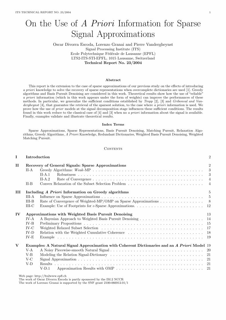
C. Example: Use of Footprints for ε-Sparse Approximations.
To give an example of the approximation of signals using a priori information, we consider again the case presentedin [1] where a piecewise-smooth signal is represented by means of an overcomplete dictionary composed by the mixtureof an orthonormal wavelet basis and a family of wavelet footprints (see [16]).
Wavelet+Footprints Dictionary
Function index
Tem
pora
l Axi
s
Fig. 1. Dictionary formed by the Symmlet-4 [17] (left half) and its respective footprints for piecewise constant singularities (right half).
Let us remind the considerations for the dictionary. The dictionary is built by the union of an orthonormal basisdefined by the Symmlet-4 family of wavelets [17] and the respective family of footprints for all the possible translationsof the Heaviside function. The latter is used to model the discontinuities. The graphical representation of the dictionarymatrix can be seen in Fig. 1 where the columns are the waveforms that compose the dictionary.
20 40 60 80 100 120−2
−1
0
1
2
3
4
5Original
temporal axis
ampl
itude
20 40 60 80 100 120−2
−1
0
1
2
3
4
5Use of OMP with dictionary D without "a priory" (10 terms approx).
temporal axis
ampl
itude
20 40 60 80 100 120−2
−1
0
1
2
3
4
5Use of OMP with dictionary D with "a priory" (10 terms approx).
temporal axis
ampl
itude
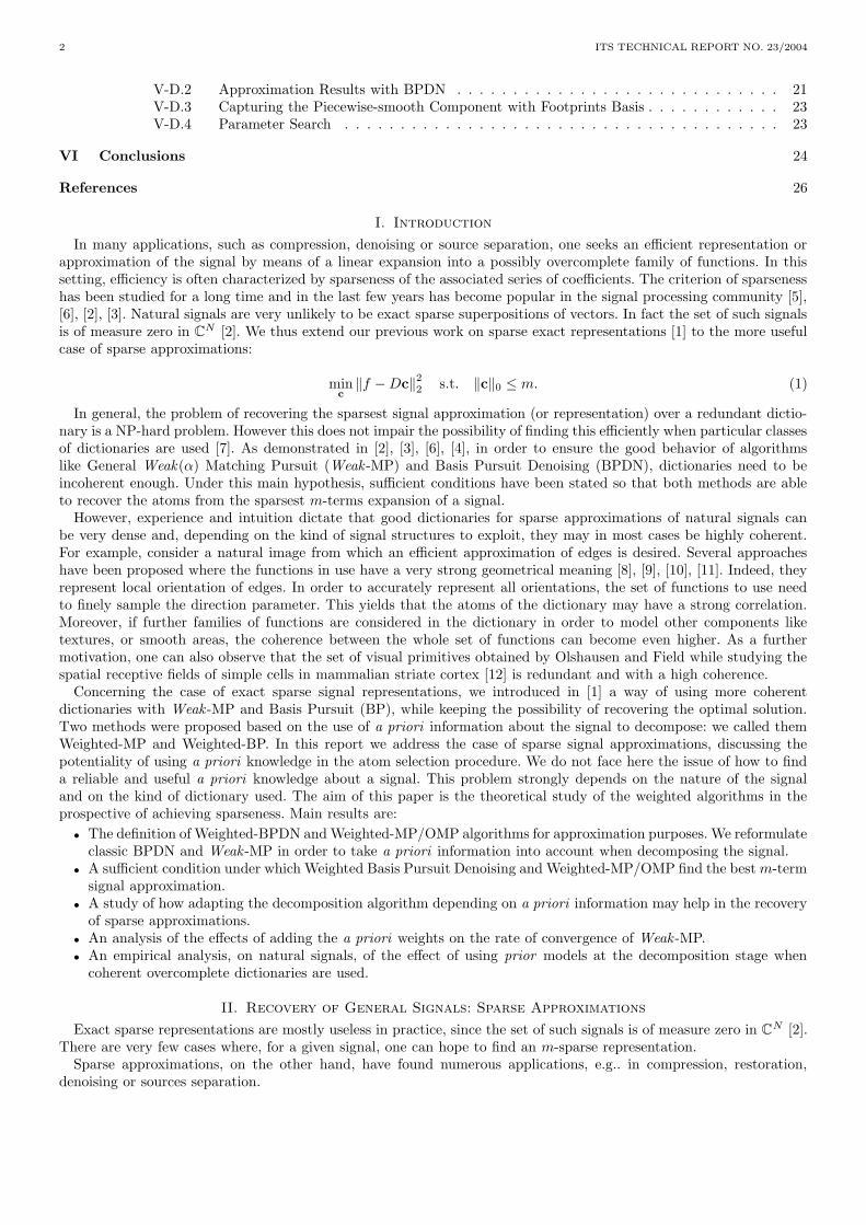
Fig. 2. Comparison of OMP based approximation with 10 terms using the footprints dictionary (Fig. 1). Left: Original signal. Middle:“blind” OMP approximation. Right: OMP with prior knowledge of the footprints location.
The use of such a dictionary, indeed, does not satisfy at all the sufficient condition required to ensure the recovery ofan optimal approximant with more than one term. Moreover, even if the best a priori was available, it is also far fromsatisfying the sufficient condition based on the weighted Babel function. Nevertheless, such an example is considered inthis section because of two main reasons. The first concerns the fact that sufficient theoretical conditions exposed in theliterature are very pessimistic and reflect the worst possible case. The second reason is that, as previously discussed,experience seems to teach us that good dictionaries for efficient approximation of signals, are likely to be highly coherent.This fact conflicts with the requirement of incoherence for the good behavior of greedy algorithms. Hence, we find thisexample of special interest to underline the benefits of using a priori information and additional signal modelingfor non-linear expansions. Indeed, with this example it is shown that, by using reliable a priori knowledge, betterapproximations are possible, not only with incoherent dictionaries (where theoretical evidences of the improvementhave been shown in this paper) but also with highly coherent ones.

DIVORRA, GRANAI AND VANDERGHEYNST 13
We repeat the procedure used in [1] to estimate the a priori information based on the dictionary and the input data.We also refer the reader to Sec. V for a more detailed explanation.
10 20 30 40 50 60 70 8010−5
10−4
10−3
10−2
10−1
100
101
102Rate of convergence of the residual error
iteration #
resi
dual
ene
rgy
OMP with a prioriOMP
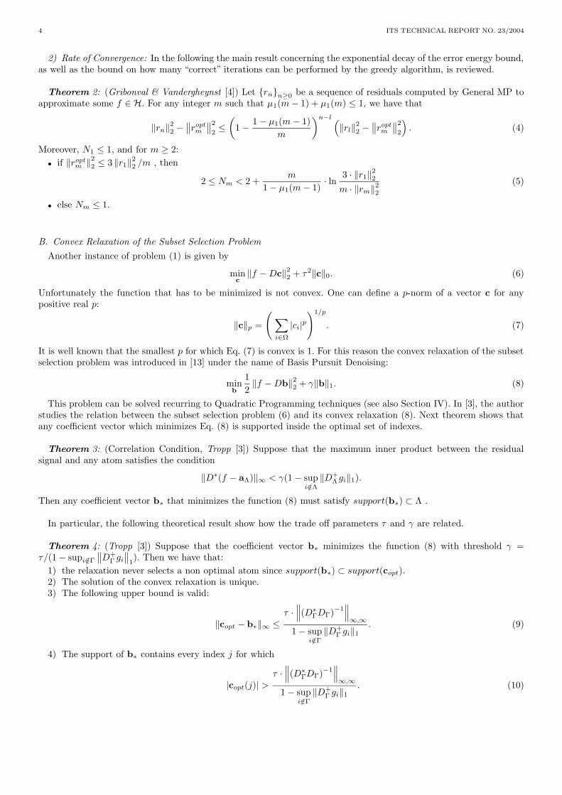
Fig. 3. Rate of convergence of the error with respect to the iteration number in the experiment of Fig. 2
Fig. 2 presents the original signal (left) together with the two approximations obtained in this example: without apriori in the middle and with a priori at the right. The signal to be approximated has a higher number of polynomialdegrees than the number of vanishing moments of the Symmlet-4. The figures depict clearly the positive effect of thereliable a priori information inserted in the Weighted-OMP algorithm. Indeed, with very few components, the algorithmbenefits from the a priori information estimated from the signal, and gives a much better approximation. A more globalview of this behavioral enhancement can be seen in Fig. 3 where the rate of convergence of the approximation erroris presented. The use of weights is definitively helpful and a considerable gain in the reduction of the approximationerror is achieved for a small number of terms.
IV. Approximations with Weighted Basis Pursuit Denoising
In this section, the problem of finding a sparse approximation of a signal f is addressed considering a trade-offbetween the error and the number of elements that participate to the approximation. In statistics this problem is alsocalled Subset Selection and we will refer to it as P0:
(P0) minc
‖f − Dc‖22 + τ2‖c‖0. (46)
Solving P0 is NP complex, so a possible way of simplifying the computation can be to substitute the `0 quasi-normwith the convex `1 norm. This relaxation leads to the following problem that, from now on, is called P1:
(P1) minb
1
2‖f − Db‖2
2 + γ‖b‖1. (47)
This new problem corresponds to the minimization of a convex function that can be solved with classical QuadraticProgramming methods. This relaxation is similar to the one that leads to the definition of the Basis Pursuit principlefor the case of exact signal representation. The fact that this paradigm is also called Basis Pursuit Denoising can beexplained because it was introduced to adapt BP to the case of noisy data [13]. Note that if D is orthonormal thesolution of P1 can be found by a soft shrinkage of the coefficients [15], [13], while, if D is a union of orthonormalsubdictionaries, the problem can be solved recurring to the Block Coordinate Relaxation method [18], faster thanQuadratic Programming.
In [1] we introduced a theoretical framework for sparse representation over redundant dictionaries taking into accountsome a priori information about the signal. In this optic we proposed the Weighted Basis Pursuit method that minimizesa cost function that includes weights expressing the a priori information:
minb
‖W−1b‖1 s.t. Db = f. (48)
The main results in [1] concerning WBP are contained in Proposition 1:
Definition 4: Given a dictionary D indexed in Ω and an index subset Λ ⊂ Ω, we define the Weighted RecoveryFactor (WRF) as:
WRF (Λ) = supi/∈Λ
∥
∥
∥(DΛWΛ)
+gi · wi
∥
∥
∥
1. (49)
14 ITS TECHNICAL REPORT NO. 23/2004
Proposition 1: Given a dictionary D and an a priori matrix W (f,D), Weighted Basis Pursuit is able to recoverthe optimal representation of a sparse signal f = DΓbΓ if the following Exact Recovery Condition is respected:
WRF (Γ) < 1. (50)
Moreover, a bound for the WRF is:
WRF (Γ) <µw
1 (m)
1 − εmax − µw1 (m − 1)
, (51)
where εmax = supγ∈Γ
∣
∣1 − w2γ
∣
∣ and wγ are the elements of the diagonal matrix WΓ. Therefore, the Exact Recovery Condition
for WBP (50) holds for any index set Γ of size at most m such that
µw1 (m) + µw
1 (m − 1) < 1 − εmax. (52)
A. A Bayesian Approach to Weighted Basis Pursuit Denoising
In this subsection the problem of signal approximation is studied from a Bayesian point of view. We also examineunder which hypotheses BPDN finds the optimal solution. This leads us to generalize the BPDN principle thorugh thedefinition of Weighted Basis Pursuit Denoising (WBPDN). Let us write again the model of our data approximation,where f is the approximant and r is the residual:
f = f + r = Db + r. (53)
Assuming r to be an iid Gaussian set of variables, the data likelihood is
p(f |D,b) =1
√
2πσ2r
· exp
(
−‖f − Db‖22
2σ2r
)
, (54)
where σ2r is the variance of the residual. In the approximation problem, one aims at maximizing the likelihood of
p(b|f,D). Formally, by the Bayes rule, we have
p(b|f,D) =p(f |D,b) · p(b)
p(f,D),
and thus, assuming p(f,D) to be uniform, it follows that the most probable signal representation is:
bP = arg maxb
p(f |D,b) · p(b). (55)
Let us now assume the coefficients bi are independent and have a Laplacian distribution with standard deviation σi:
p(bi) =1√2σi
· exp
(
−√
2|bi|σi
)
From (55), by computing the logarithm, it follows that
bP = arg maxb
(
ln(p(f |D,b)) +∑
i
ln p(bi)
)
= arg minb
(
‖f − Db‖22
2σ2r
+∑
i
√2|bi|σi
)
.
Making the hypothesis that σi is constant for every index i, the previous equation means that the most probable bis the one found by the BPDN algorithm [19]. In fact, this hypothesis does not often correspond to reality. On thecontrary, if the variances of the coefficients are not forced to be all the same, it turns out that the most probable signalrepresentation can be found by solving the following problem:
(Pw1 ) min
b
1
2‖f − Db‖2
2 + γ‖W−1b‖1, (56)
where the diagonal matrix with entries in (0, 1] is defined in Section III. One can notice that in Eq. (56), the introductionof weights allows to individually model the components of b. This approach is analogous to the one introduced in [20]and [1] and, from now on, we will refer to P w
1 as Weighted Basis Pursuit Denoising or WBPDN.The assumption often made about the Gaussianity of the residual is quite restrictive. However, for another particular
problem, one could make the hypothesis that this residual has a Laplacian distribution. It is then possible to provethat the most probable signal representation can be found substituting the `2 measure of the error with the `1. Thisleads to the following minimization problem:
minb
1
2‖f − Db‖1 + γ‖W−1b‖1,
where W = I if the variances of the probability density functions of bi are the same for each i. This problem is faced,for example in [20], where it is also explained that it can be solved by Linear Programming techniques.

DIVORRA, GRANAI AND VANDERGHEYNST 15
B. Preliminary Propositions
Here some preliminary propositions are presented, allowing us to prove the results of the following two subsections.The proofs of most of them follow the arguments given by Tropp in [3]. In the following cΛ and bΛ lay in R
Λ butsometimes these are extended to R
Ω by padding with zeros. The same is valid for the matrix WΛ.Next proposition, similar to the Correlation Condition Lemma in [3], establishes a fundamental result for the rest
of the report: it basically states that, if the atoms of Λ have a small weighted coherence, expressed by the WeightedRecovery Factor, then the support of any vector that solves P w
1 is a subset of Λ.
Lemma 3: Given an index subset Λ ⊂ Ω, suppose that the following condition is satisfied:
‖DT (f − aΛ)‖∞ <γ
wmaxΓ
· (1 − WRF (Λ)), (57)
where wmaxΛ
∈ (0, 1] is the quantity defined by equation (13). Then, any coefficient vector b∗ that minimizes the costfunction of problem P w
1 must satisfysupport(b∗) ⊂ Λ. (58)
Proof: Assume that b∗ is a vector minimizing (56). Assume also that it uses an index outside Λ. b∗ can be comparedwith its projection D+
ΛDb∗, which is supported in Λ and we obtain:
1
2‖f − Db∗‖2
2 + γ∥
∥W−1b∗
∥
∥
1≤ 1
2
∥
∥f − DD+ΛDb∗
∥
∥
2
2+ γ
∥
∥W−1Λ (D+
ΛDb∗)∥
∥
1,
which gives
2γ(∥
∥W−1b∗
∥
∥
1−∥
∥W−1Λ (D+
ΛDb∗)∥
∥
1
)
≤∥
∥f − DD+ΛDb∗
∥
∥
2
2− ‖f − Db∗‖2
2 . (59)
First we shall provide a lower bound on the left-hand side of the previous inequality. Let us split the vector b∗ intotwo parts: b∗ = bΛ + bΛ, where the former vector contains the components with indexes in Λ, while the latter theremaining components from Ω \ Λ. This yields, by the upper triangular inequality, that
∥
∥W−1b∗
∥
∥
1−∥
∥W−1Λ (D+
ΛDb∗)∥
∥
1=∥
∥W−1bΛ
∥
∥
1+∥
∥W−1bΛ
∥
∥
1−∥
∥W−1bΛ + W−1Λ D+
ΛDbΛ
∥
∥
1
≥∥
∥W−1bΛ
∥
∥
1−∥
∥W−1Λ D+
ΛDWW−1bΛ
∥
∥
1.
Since∥
∥W−1Λ D+
ΛDWW−1bΛ
∥
∥
1≤ sup
i/∈Λ
∥
∥
∥(DΛWΛ)+
giwi
∥
∥
∥
1·∥
∥W−1bΛ
∥
∥
1,
using (49), one can write that∥
∥W−1b∗
∥
∥
1−∥
∥W−1Λ (D+
ΛDb∗)∥
∥
1≥ (1 − WRF (Λ)) ·
∥
∥W−1bΛ
∥
∥
1. (60)
We now provide an upper bound for the right-hand side of (59). This quantity does not depend on the weightingmatrix, thus, exactly as in [3], it can be stated that:
∥
∥f − DD+ΛDb∗
∥
∥
2
2− ‖f − Db∗‖2
2 ≤ 2‖bΛ‖1 ·∥
∥DT (f − aΛ)∥
∥
∞. (61)
From (59), (60) and (61) it turns out that:
γ (1 − WRF (Λ)) ·∥
∥W−1bΛ
∥
∥
1≤ ‖bΛ‖1
·∥
∥DT (f − aΛ)∥
∥
∞. (62)
Since the weights are in (0, 1], and the vector bΓ, by assumption, cannot be null, it can be written:
γ (1 − WRF (Λ)) ≤ ‖bΛ‖1
‖W−1bΛ‖1
·∥
∥DT (f − aΛ)∥
∥
∞≤ wmax
Λ·∥
∥DT (f − aΛ)∥
∥
∞. (63)
If (57) is valid , then (63) fails and so one must discard the hypothesis that b∗ is non-zero for an index in Λ = Ω \ Λ.
We now focus on finding a necessary and sufficient condition for the existence and unicity of a minimum of P w1 . The
presence of the `1 norm imply that the cost function of this problem is non-smooth at zero: for this reason the conceptof subdifferential is used. Given a real vector variable x, the subdifferential of ‖x‖1 is denoted by ∂‖x‖1 and definedas:
∂‖x‖1 , u|u∗x = ‖x‖1, ‖u‖∞ ≤ 1 .
The vectors u that compose the subdifferential are called subgradients [21].
16 ITS TECHNICAL REPORT NO. 23/2004
Lemma 4: A necessary and sufficient condition for b∗ to globally minimize the objective function of P w1 over all
the coefficient vectors with support Λ is that:
cΛ − b∗ = γ(
DTΛDΛ
)−1W−1
Λ u, (64)
where u is a vector from ∂‖b∗‖1. Moreover, the minimizer is unique.
Proof: One can observe that solving P w1 is equivalent to minimize the following function over coefficient vectors
from RΛ:
F (b) ,1
2‖aΛ − DΛb‖2
2 + γ‖W−1Λ b‖1.
A point b∗ minimizes the second term of F (b) if and only if the following Fermat criterion holds (see [21], [22]):
0 ∈ ∂‖b∗‖1.
Moreover, b∗ minimizes F (b) if and only if 0 ∈ ∂F (b∗). In our case this means that
∃ u ∈ ∂‖b∗‖1 s.t. DTΛDΛb∗ − DT
ΛaΛ + γW−1Λ u = 0, (65)
for some vector u taken from ∂‖b∗‖1. Let the atoms in Λ be linearly independent, from (65) it follows:
b∗ −(
DTΛDΛ
)−1DT
ΛaΛ + γ(
DTΛDΛ
)−1W−1
Λ u = 0,
and so
D+ΛaΛ − b∗ = γ
(
WΛDTΛDΛ
)−1u.
To conclude the proof it is sufficient to recall that cΛ = D+ΛaΛ.
If W = I, then this result coincides with the one developed by Fuchs in [23] and by Tropp in [3] in the complex case.
Lemma 5: Suppose that b∗ minimizes the cost function of problem P w1 . Then the following bound holds:
‖cΛ − b∗‖∞ ≤ γ
wminΛ
·∥
∥
∥
(
DTΛDΛ
)−1∥
∥
∥
∞,∞, (66)
where wminΛ is defined as
wminΛ , inf
i∈Λwi. (67)
Proof: Let us consider the necessary and sufficient condition of Lemma 4: taking the `∞ norm of (64) we obtain:
‖cΛ − b∗‖∞ = γ∥
∥
∥
(
DTΛDΛ
)−1W−1
Λ u∥
∥
∥
∞≤ γ
∥
∥
∥
(
DTΛDΛ
)−1W−1
Λ
∥
∥
∥
∞,∞· ‖u‖∞
By definition of subdifferential, ‖u‖∞ ≤ 1. Inserting this into the previous equation and using the sub-multiplicativeproperty of matrix norms (‖AB‖p,q ≤ ‖A‖p,q · ‖B‖p,q), we can prove that
‖cΛ − b∗‖∞ ≤ γ∥
∥
∥
(
DTΛDΛ
)−1∥
∥
∥
∞,∞·∥
∥W−1Λ
∥
∥
∞,∞.
Just apply the fact that∥
∥W−1Λ
∥
∥
∞,∞= sup
i∈Λ(1/wi) =
1
wminΛ
to reach the result.
The following proposition states a result that will be used in next subsection to prove Theorem 8. Note that here Γis the optimal index subset of Ω, and thus cΓ is the sparsest solution to the subset selection problem.
Proposition 2: (Tropp [3]) Given an input signal f and a threshold τ , suppose that the coefficient vector cΓ, havingsupport Γ of cardinality m, is the sparsest solution of the problem P0. Set fopt
m = DcΓ. Then:
• ∀k ∈ Γ, |cΓ(k)| ≥ τ .• ∀i /∈ Γ, |〈f − fopt
m , gi〉| < τ .
These preliminary statements of this subsection will allow us to obtain the main results in the following of the report.
DIVORRA, GRANAI AND VANDERGHEYNST 17
C. Weighted Relaxed Subset Selection
Let us now study the relationship between the results obtained by solving problem P w1 and P0. Suppose that cΓ is
the sparsest solution to P0 and that its support is Γ, with |Γ| = m. DΓ will be the matrix containing all the atomsparticipating to the sparsest approximation of f and f opt
m will be the approximant given by cΓ, i.e foptm = Dcopt =
DD+Γ f = DΓD+
Γ f . Assuming WRF (Γ) < 1, we have the following result.
Theorem 8: Suppose that b∗ minimizes the cost function of problem P w1 with threshold
γ =τ · wmax
Γ
1 − WRF (Γ),
where wmaxΓ
is defined in (13). Then:
1) WBP never selects a non optimal atom since support(b∗) ⊂ Γ.2) The solution of WBP is unique.3) The following upper bound is valid:
‖cΓ − b∗‖∞ ≤τ · wmax
Γ
wmin
Γ
·∥
∥
∥
(
DTΓ DΓ
)−1∥
∥
∥
∞,∞
1 − WRF (Γ). (68)
4) The support of b∗ contains every index j for which
|cΓ(j)| >τ · wmax
Γ
wmin
Γ
·∥
∥
∥
(
DTΓ DΓ
)−1∥
∥
∥
∞,∞
1 − WRF (Γ). (69)
The scalar wminΓ appearing in Eqs. (68) and (69) is defined in Eq. (67).
Proof: Considering the first stated result, note that every atom indexed by Γ has zero inner product with theoptimal residual (ropt
m = f − foptm ) since fopt
m is the best approximation of f using the atoms in Γ. Using Proposition 2and recalling that D is finite, it can be stated that
∥
∥DT (f − foptm )
∥
∥
∞< τ. (70)
Moreover, Lemma 3 guarantees that
∀γ s.t.∥
∥DT (f − foptm )
∥
∥
∞<
γ
wmaxΓ
· (1 − WRF (Γ)), (71)
and that the solution b∗ to the convex problem P w1 is supported on Γ. From (70) and (71) it follows that for any γ
that satisfies the following condition, it is insured that support(b∗) ⊂ Γ:
γ ≥τ · wmax
Γ
1 − WRF (Γ). (72)
In the following, the smallest possible value for γ is chosen: in this way, Eq. (72) becomes an equality.The uniqueness of the solution follows from Lemma 4.With regard to the third point, the results from Lemma 5 yield
‖cΓ − b∗‖∞ ≤ γ
wminΓ
∥
∥
∥
(
DTΓ DΓ
)−1∥
∥
∥
∞,∞≤
τ · wmax
Γ
wmin
Γ
1 − WRF (Γ)·∥
∥
∥
(
DTΓ DΓ
)−1∥
∥
∥
∞,∞.
This proves the point 3.Concerning the fourth result of the theorem, one can observe that, for every index j for which
|cΓ(j)| > γ∥
∥
∥
(
DTΓ DΓ
)−1W−1
Γ
∥
∥
∥
∞,∞,
the corresponding coefficient b∗(j) must be different form zero. As before, substituting Eq. (72) leads to prove the lastresult of the Theorem.
This theorem states two important concepts. First, if the trade off parameter is correct and the weighted cumulativecoherence of the dictionary is small enough, WBPDN is able to select the correct atoms for the signal expansionand it will not pick up the wrong ones. Furthermore, the error achieved by the algorithm on the amplitude of thecoefficients related to the selected atoms is bounded. Nevertheless, once the algorithm has recovered the atom subset,the appropriate amplitudes of the coefficients can be computed by the orthogonal projection of the signal onto thespace generated by the selected atoms. This method is illustrated in Section IV-E to generate some examples.
18 ITS TECHNICAL REPORT NO. 23/2004
The quantities wminΓ and wmax
Γdepend on the reliability and goodness of the a priori. In particular, if W tends to
be optimal (i.e. its diagonal entries tend to 1 for the elements that should appear in the sparsest approximation andto 0 for the ones that should not), one can observe that wmin
Γ → 1 and wmaxΓ
→ 0.
D. Relation with the Weighted Cumulative Coherence
In this subsection, the previous results are described using the weighted cumulative coherence function defined in(15). In this way a comparison is made between the results achievable by BPDN and WBPDN.
Theorem 9: Assume that the real vector b∗ solves P w1 with
γ =wmax
Γ· τ(1 − εmax − µw
1 (m − 1))
1 − εmax − µw1 (m) − µw
1 (m − 1).
Then support(b∗) ⊂ Γ and
‖b∗ − cΓ‖∞ ≤τ · wmax
Γ
wmin
Γ
(1 − εmax − µw1 (m − 1))
(1 − εmax − µw1 (m) − µw
1 (m − 1))(1 − µ1(m − 1)). (73)
Proof: This result can be obtained from Proposition 1 and Theorem 8, since:
‖b∗ − cΓ‖∞ ≤ γ
wminΓ
∥
∥
∥
(
DTΓ DΓ
)−1∥
∥
∥
∞,∞=
τ · wmax
Γ
wmin
Γ
(1 − εmax − µw1 (m − 1)) ·
∥
∥
∥
(
DTΓ DΓ
)−1∥
∥
∥
∞,∞
(1 − εmax − µw1 (m) − µw
1 (m − 1)).
The last term of the numerator in the previous expression is the norm of the inverse Gram matrix. Since
‖(
DTΓ DΓ
)−1 ‖∞,∞ = ‖(
DTΓ DΓ
)−1 ‖1,1 ≤ 1
1 − µ1(m − 1),
(see [3], [23], [1]) this proves equation (73).
This result is valid in general and illustrates how the distance between the optimal signal approximation and thesolution found by solving P w
1 can be bounded. In case no a priori is given, the bound on the coefficient error is obtainedfrom Eq. (73) setting W = I. Consequently, wmin
Γ = 1, εmax = 0 and wmaxΓ
= 1 (see also [3]):
‖b∗ − cΓ‖∞ ≤ τ
1 − µ1(m) − µ1(m − 1). (74)
Comparing the two bounds, one can observe how the availability of a reliable prior on the signal can help in finding asparser signal approximation. This concept is emphasized in the following corollary.
Corollary 3: Let W (f,D) be a reliable a priori knowledge, with
wmaxΓ
wminΓ
≤ 1,
then for any positive integer m such that µ1(m−1)+µ1(m) < 1 and µw1 (m−1)+µw
1 (m)+εmax < µ1(m−1)+µ1(m) < 1,the error ‖b∗ − cΓ‖∞ given by the coefficients found by WBPDN is smaller than the one obtained by BPDN.
Hence, the bound stated by Eq. (73) is lower than the one in Eq. (74), i.e.
τ · wmax
Γ
wmin
Γ
(1 − εmax − µw1 (m − 1))
(1 − εmax − µw1 (m) − µw
1 (m − 1))(1 − µ1(m − 1))≤ τ
1 − µ1(m) − µ1(m − 1).
Note the similarity between Corollaries 2 and 3. The proof of the latter Corollary is reported in the appendix. Here
the hypothesis thatwmax
Γ
wmin
Γ
≤ 1 is made. Observe that if the a priori is particularly good this factor can be much smaller
than one and so the improvement with respect to the general case can be really big.
DIVORRA, GRANAI AND VANDERGHEYNST 19
E. Example
We examine again the example presented in section III-C, but this time using the Basis Pursuit Denoising andWeighted Basis Pursuit Denoising algorithms. The dictionary used for the decomposition is illustrated in section III-C,as well as the input signal. For an explanation of the prior model and the extraction of the a priori matrix, see [1] orSection V.
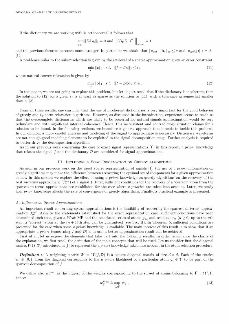
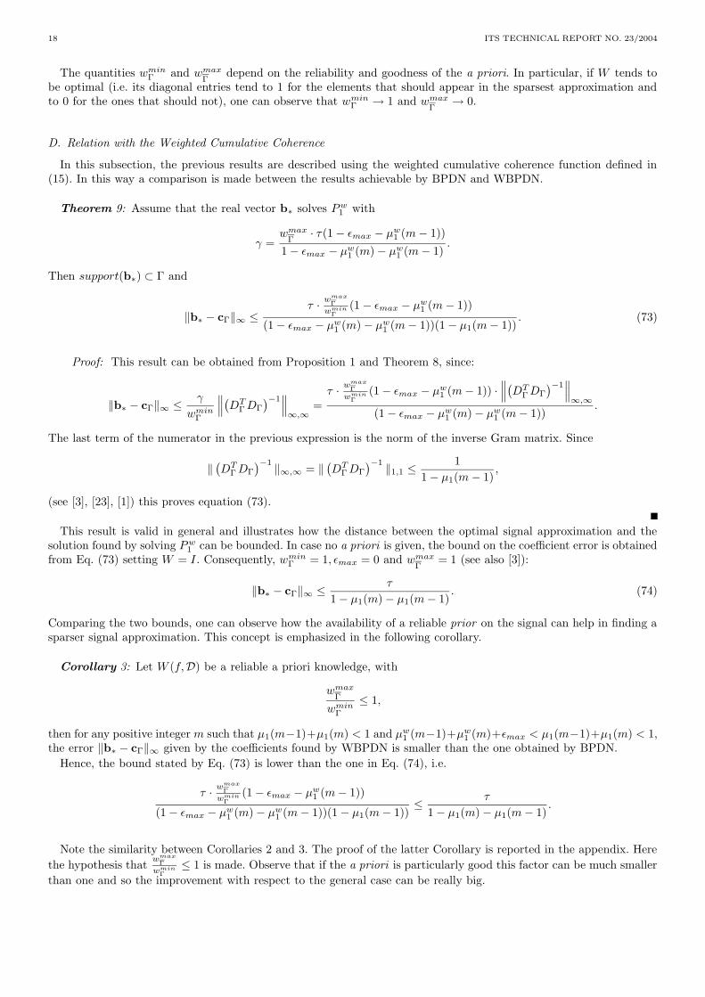
The signal f is decomposed first solving the minimization problem illustrated in (47) (BPDN). Then, the a prioriknowledge is introduced, and we solve the minimization problem illustrated in (56) (WBPDN). Both solutions werenumerically found using Quadratic Programming techniques. The trade off parameter γ controls the `1 norm of thecoefficient vector and indirectly its sparseness. The signal representations present many components with negligiblevalues due to the numerical computation: a hard thresholding is performed in order to get rid of this misleadinginformation, paying attention not to eliminate significant elements. In this optic it is possible to measure the `0 normof the vector b. The data reported here refer to a threshold value of 0.01. Of course the reconstructions are computedstarting from the thresholded coefficients. Figure 4 shows the reconstructions of the input signal given by a 10-termsapproximation found by BPDN and WBPDN. Figure 6 (on the left-hand) illustrates the mean square error of the
20 40 60 80 100 120−2
−1
0
1
2
3
4
5Original
temporal axis
ampl
itude
20 40 60 80 100 120−2
−1
0
1
2
3
4
5reconstructed by BP: 10 terms
temporal axis
ampl
itude
20 40 60 80 100 120−2
−1
0
1
2
3
4
5reconstructed by WBP: 10 terms
temporal axis
ampl
itude
Fig. 4. Comparison of BPDN and WBPDN based approximation with 10 terms using the footprints dictionary (Fig. 1). Left: Originalsignal. Center: reconstruction using 10 BPDN coefficients. Right: reconstruction using 10 WBPDN coefficients.
approximations of f with m terms found by BPDN and WBPDN.
Let us call b∗ the approximation found by BPDN and bw∗ the one found by WBPDN. As just explained, these vectors
are thresholded removing the numerically negligible components, and in this way we are able to individuate a sparsesupport and so a subset of the dictionary. Let us label the subdictionary found by WBPDN with Dw
∗ (composed by theatoms corresponding to the non-zero elements of bw
∗ ). Once this is given, there are no guarantees that the coefficientsthat represent f are optimal (see Theorems 8 and 4). These are, thus, recomputed projecting the signal onto Dw
∗ anda new approximation of f named bw
∗∗ is found. Exactly the same is done for BPDN, ending up with a subdictionaryD∗ and a new approximation b∗∗. Of course, support(b∗) = support(b∗∗) and support(bw
∗ ) = support(bw∗∗). Formally
the approximants found by BPDN and WBPDN are respectively:
f∗∗ = D∗D+∗ f = Db∗∗ and
fw∗∗ = Dw
∗ (Dw∗ )+f = Db∗∗.
(75)
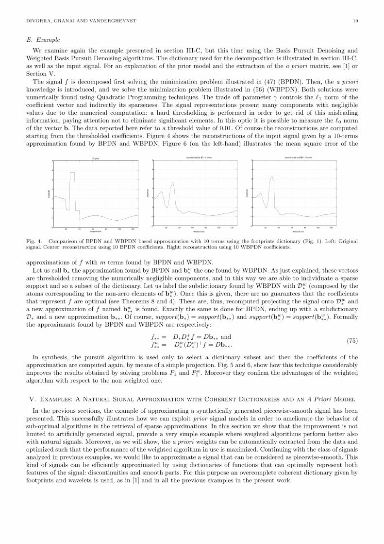
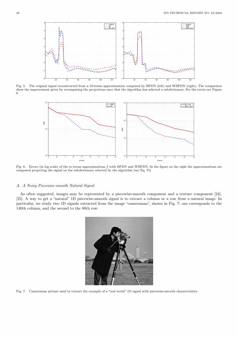
In synthesis, the pursuit algorithm is used only to select a dictionary subset and then the coefficients of theapproximation are computed again, by means of a simple projection. Fig. 5 and 6, show how this technique considerablyimproves the results obtained by solving problems P1 and Pw
1 . Moreover they confirm the advantages of the weightedalgorithm with respect to the non weighted one.
V. Examples: A Natural Signal Approximation with Coherent Dictionaries and an A Priori Model
In the previous sections, the example of approximating a synthetically generated piecewise-smooth signal has beenpresented. This successfully illustrates how we can exploit prior signal models in order to ameliorate the behavior ofsub-optimal algorithms in the retrieval of sparse approximations. In this section we show that the improvement is notlimited to artificially generated signal, provide a very simple example where weighted algorithms perform better alsowith natural signals. Moreover, as we will show, the a priori weights can be automatically extracted from the data andoptimized such that the performance of the weighted algorithm in use is maximized. Continuing with the class of signalsanalyzed in previous examples, we would like to approximate a signal that can be considered as piecewise-smooth. Thiskind of signals can be efficiently approximated by using dictionaries of functions that can optimally represent bothfeatures of the signal: discontinuities and smooth parts. For this purpose an overcomplete coherent dictionary given byfootprints and wavelets is used, as in [1] and in all the previous examples in the present work.
20 ITS TECHNICAL REPORT NO. 23/2004
20 40 60 80 100 120−2
−1
0
1
2
3
4
5originalBPBP+proj
20 40 60 80 100 120−2
−1
0
1
2
3
4
5originalWBPWBP+proj
Fig. 5. The original signal reconstructed from a 10-terms approximation computed by BPDN (left) and WBPDN (right). The comparisonshow the improvement given by recomputing the projections once that the algorithm has selected a subdictionary. For the errors see Figure6
5 6 7 8 9 10 11 12 1310−2
10−1
100
# terms
MS
E
WBPBP
6 7 8 9 10 11 12 1310−3
10−2
10−1
100
# terms
MS
E
BP + projWBP + proj
Fig. 6. Errors (in log scale) of the m-terms approximations f with BPDN and WBPDN. In the figure on the right the approximations arecomputed projecting the signal on the subdictionary selected by the algorithm (see Eq. 75)
A. A Noisy Piecewise-smooth Natural Signal
As often suggested, images may be represented by a piecewise-smooth component and a texture component [24],[25]. A way to get a “natural” 1D piecewise-smooth signal is to extract a column or a row from a natural image. Inparticular, we study two 1D signals extracted from the image “cameraman”, shown in Fig. 7: one corresponds to the140th column, and the second to the 80th row.
Fig. 7. Cameraman picture used to extract the example of a “real world” 1D signal with piecewise-smooth characteristics
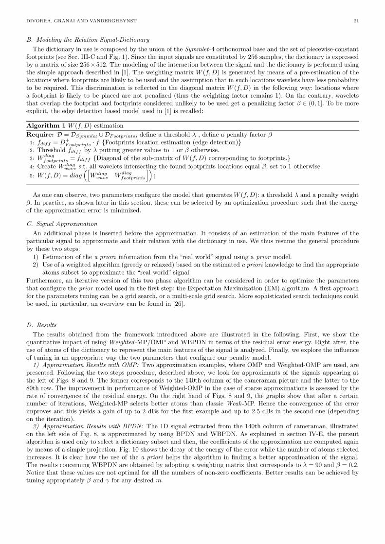
DIVORRA, GRANAI AND VANDERGHEYNST 21
B. Modeling the Relation Signal-Dictionary
The dictionary in use is composed by the union of the Symmlet-4 orthonormal base and the set of piecewise-constantfootprints (see Sec. III-C and Fig. 1). Since the input signals are constituted by 256 samples, the dictionary is expressedby a matrix of size 256×512. The modeling of the interaction between the signal and the dictionary is performed usingthe simple approach described in [1]. The weighting matrix W (f,D) is generated by means of a pre-estimation of thelocations where footprints are likely to be used and the assumption that in such locations wavelets have less probabilityto be required. This discrimination is reflected in the diagonal matrix W (f,D) in the following way: locations wherea footprint is likely to be placed are not penalized (thus the weighting factor remains 1). On the contrary, waveletsthat overlap the footprint and footprints considered unlikely to be used get a penalizing factor β ∈ (0, 1]. To be moreexplicit, the edge detection based model used in [1] is recalled:
Algorithm 1 W (f,D) estimation
Require: D = DSymmlet ∪ DFootprints, define a threshold λ , define a penalty factor β1: fdiff = D+
Footprints · f Footprints location estimation (edge detection)2: Threshold fdiff by λ putting greater values to 1 or β otherwise.
3: W diagfootprints = fdiff Diagonal of the sub-matrix of W (f,D) corresponding to footprints.
4: Create W diagwave s.t. all wavelets intersecting the found footprints locations equal β, set to 1 otherwise.
5: W (f,D) = diag([
W diagwave W diag
footprints
])
;
As one can observe, two parameters configure the model that generates W (f,D): a threshold λ and a penalty weightβ. In practice, as shown later in this section, these can be selected by an optimization procedure such that the energyof the approximation error is minimized.
C. Signal Approximation
An additional phase is inserted before the approximation. It consists of an estimation of the main features of theparticular signal to approximate and their relation with the dictionary in use. We thus resume the general procedureby these two steps:
1) Estimation of the a priori information from the “real world” signal using a prior model.2) Use of a weighted algorithm (greedy or relaxed) based on the estimated a priori knowledge to find the appropriate
atoms subset to approximate the “real world” signal.
Furthermore, an iterative version of this two phase algorithm can be considered in order to optimize the parametersthat configure the prior model used in the first step: the Expectation Maximization (EM) algorithm. A first approachfor the parameters tuning can be a grid search, or a multi-scale grid search. More sophisticated search techniques couldbe used, in particular, an overview can be found in [26].
D. Results
The results obtained from the framework introduced above are illustrated in the following. First, we show thequantitative impact of using Weighted -MP/OMP and WBPDN in terms of the residual error energy. Right after, theuse of atoms of the dictionary to represent the main features of the signal is analyzed. Finally, we explore the influenceof tuning in an appropriate way the two parameters that configure our penalty model.
1) Approximation Results with OMP: Two approximation examples, where OMP and Weighted-OMP are used, arepresented. Following the two steps procedure, described above, we look for approximants of the signals appearing atthe left of Figs. 8 and 9. The former corresponds to the 140th column of the cameraman picture and the latter to the80th row. The improvement in performance of Weighted-OMP in the case of sparse approximations is assessed by therate of convergence of the residual energy. On the right hand of Figs. 8 and 9, the graphs show that after a certainnumber of iterations, Weighted-MP selects better atoms than classic Weak -MP. Hence the convergence of the errorimproves and this yields a gain of up to 2 dBs for the first example and up to 2.5 dBs in the second one (dependingon the iteration).
2) Approximation Results with BPDN: The 1D signal extracted from the 140th column of cameraman, illustratedon the left side of Fig. 8, is approximated by using BPDN and WBPDN. As explained in section IV-E, the pursuitalgorithm is used only to select a dictionary subset and then, the coefficients of the approximation are computed againby means of a simple projection. Fig. 10 shows the decay of the energy of the error while the number of atoms selectedincreases. It is clear how the use of the a priori helps the algorithm in finding a better approximation of the signal.The results concerning WBPDN are obtained by adopting a weighting matrix that corresponds to λ = 90 and β = 0.2.Notice that these values are not optimal for all the numbers of non-zero coefficients. Better results can be achieved bytuning appropriately β and γ for any desired m.
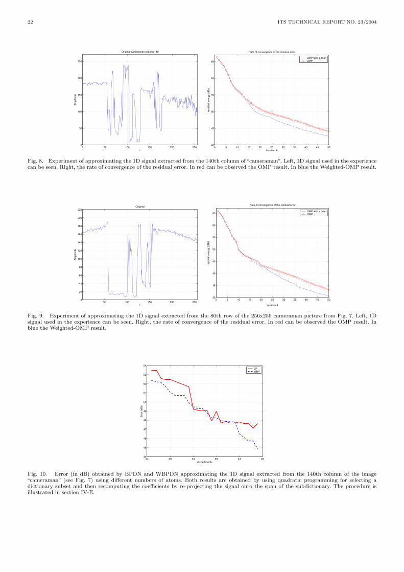
22 ITS TECHNICAL REPORT NO. 23/2004
0 50 100 150 200 2500
50
100
150
200
250
Original cameraman column 140
t
Am
plitu
de
0 5 10 15 20 25 30 35 40 45 5040
45
50
55
60
65
Rate of convergence of the residual error
iteration #
resi
dual
ene
rgy
(dB
s)
OMP with a prioriOMP
Fig. 8. Experiment of approximating the 1D signal extracted from the 140th column of “cameraman”. Left, 1D signal used in the experiencecan be seen. Right, the rate of convergence of the residual error. In red can be observed the OMP result. In blue the Weighted-OMP result.
50 100 150 200 2500
20
40
60
80
100
120
140
160
180
200
220Original
t
Am
plitu
de
0 5 10 15 20 25 30 35 40 45 5030
35
40
45
50
55
60
65
iteration #
resi
dual
ene
rgy
(dB
s)Rate of convergence of the residual error
OMP with a prioriOMP
Fig. 9. Experiment of approximating the 1D signal extracted from the 80th row of the 256x256 cameraman picture from Fig. 7. Left, 1Dsignal used in the experience can be seen. Right, the rate of convergence of the residual error. In red can be observed the OMP result. Inblue the Weighted-OMP result.
24 29 34 39 44 4944
45
46
47
48
49
50
51
52
53
54
# coefficients
Err
or (d
Bs)
BPWBP
Fig. 10. Error (in dB) obtained by BPDN and WBPDN approximating the 1D signal extracted from the 140th column of the image“cameraman” (see Fig. 7) using different numbers of atoms. Both results are obtained by using quadratic programming for selecting adictionary subset and then recomputing the coefficients by re-projecting the signal onto the span of the subdictionary. The procedure isillustrated in section IV-E.
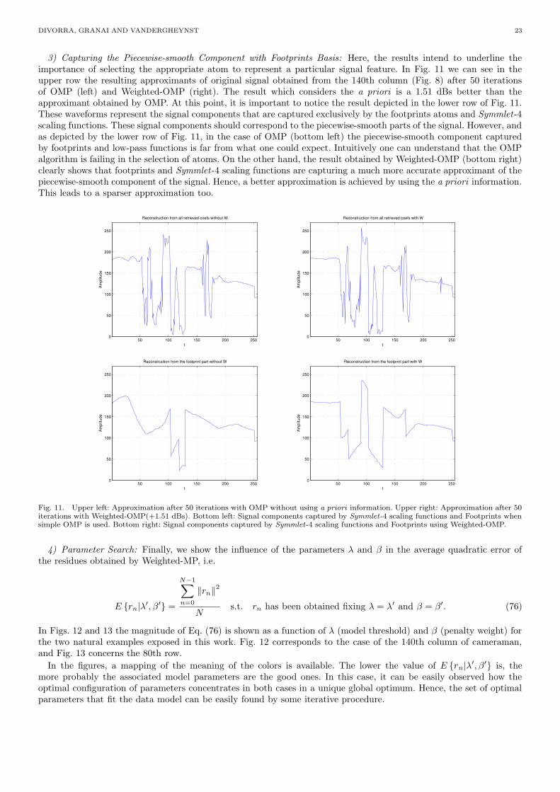
DIVORRA, GRANAI AND VANDERGHEYNST 23
3) Capturing the Piecewise-smooth Component with Footprints Basis: Here, the results intend to underline theimportance of selecting the appropriate atom to represent a particular signal feature. In Fig. 11 we can see in theupper row the resulting approximants of original signal obtained from the 140th column (Fig. 8) after 50 iterationsof OMP (left) and Weighted-OMP (right). The result which considers the a priori is a 1.51 dBs better than theapproximant obtained by OMP. At this point, it is important to notice the result depicted in the lower row of Fig. 11.These waveforms represent the signal components that are captured exclusively by the footprints atoms and Symmlet-4scaling functions. These signal components should correspond to the piecewise-smooth parts of the signal. However, andas depicted by the lower row of Fig. 11, in the case of OMP (bottom left) the piecewise-smooth component capturedby footprints and low-pass functions is far from what one could expect. Intuitively one can understand that the OMPalgorithm is failing in the selection of atoms. On the other hand, the result obtained by Weighted-OMP (bottom right)clearly shows that footprints and Symmlet-4 scaling functions are capturing a much more accurate approximant of thepiecewise-smooth component of the signal. Hence, a better approximation is achieved by using the a priori information.This leads to a sparser approximation too.
50 100 150 200 2500
50
100
150
200
250
Reconstruction from all retrieved coefs without W
t
Am
plitu
de
50 100 150 200 2500
50
100
150
200
250
Reconstruction from all retrieved coefs with W
t
Am
plitu
de
50 100 150 200 2500
50
100
150
200
250
Reconstruction from the footprint part without W
t
Am
plitu
de
50 100 150 200 2500
50
100
150
200
250
Reconstruction from the footprint part with W
t
Am
plitu
de
Fig. 11. Upper left: Approximation after 50 iterations with OMP without using a priori information. Upper right: Approximation after 50iterations with Weighted-OMP(+1.51 dBs). Bottom left: Signal components captured by Symmlet-4 scaling functions and Footprints whensimple OMP is used. Bottom right: Signal components captured by Symmlet-4 scaling functions and Footprints using Weighted-OMP.
4) Parameter Search: Finally, we show the influence of the parameters λ and β in the average quadratic error ofthe residues obtained by Weighted-MP, i.e.
E rn|λ′, β′ =
N−1∑
n=0
‖rn‖2
Ns.t. rn has been obtained fixing λ = λ′ and β = β′. (76)
In Figs. 12 and 13 the magnitude of Eq. (76) is shown as a function of λ (model threshold) and β (penalty weight) forthe two natural examples exposed in this work. Fig. 12 corresponds to the case of the 140th column of cameraman,and Fig. 13 concerns the 80th row.
In the figures, a mapping of the meaning of the colors is available. The lower the value of E rn|λ′, β′ is, themore probably the associated model parameters are the good ones. In this case, it can be easily observed how theoptimal configuration of parameters concentrates in both cases in a unique global optimum. Hence, the set of optimalparameters that fit the data model can be easily found by some iterative procedure.
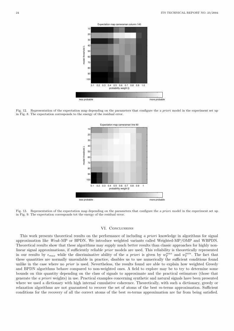
24 ITS TECHNICAL REPORT NO. 23/2004
Expectation map cameraman column 140
probability weight β
mod
el th
resh
old
λ0.1 0.2 0.3 0.4 0.5 0.6 0.7 0.8 0.9 1.0
10
20
30
40
50
60
70
80
90
100
less probable more probable
Fig. 12. Representation of the expectation map depending on the parameters that configure the a priori model in the experiment set upin Fig. 8. The expectation corresponds to the energy of the residual error.
Expectation map cameraman line 80
probability weight β
mod
el th
resh
old
λ
0.1 0.2 0.3 0.4 0.5 0.6 0.7 0.8 0.9 1
10
20
30
40
50
60
70
80
90
100
less probable more probable
Fig. 13. Representation of the expectation map depending on the parameters that configure the a priori model in the experiment set upin Fig. 9. The expectation corresponds tot the energy of the residual error.
VI. Conclusions
This work presents theoretical results on the performance of including a priori knowledge in algorithms for signalapproximation like Weak -MP or BPDN. We introduce weighted variants called Weighted-MP/OMP and WBPDN.Theoretical results show that these algorithms may supply much better results than classic approaches for highly non-linear signal approximations, if sufficiently reliable prior models are used. This reliability is theoretically representedin our results by εmax while the discriminative ability of the a priori is given by wmax
Γand wmin
Γ . The fact thatthese quantities are normally unavailable in practice, disables us to use numerically the sufficient conditions foundunlike in the case where no prior is used. Nevertheless, the results found are able to explain how weighted Greedyand BPDN algorithms behave compared to non-weighted ones. A field to explore may be to try to determine somebounds on this quantity depending on the class of signals to approximate and the practical estimators (those thatgenerate the a priori weights) in use. Practical examples concerning synthetic and natural signals have been presentedwhere we used a dictionary with high internal cumulative coherence. Theoretically, with such a dictionary, greedy orrelaxation algorithms are not guaranteed to recover the set of atoms of the best m-terms approximation. Sufficientconditions for the recovery of all the correct atoms of the best m-terms approximation are far from being satisfied.
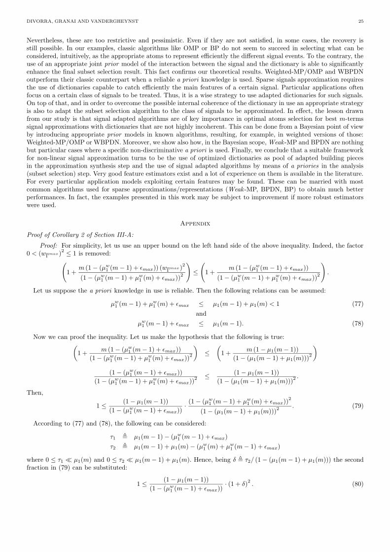
DIVORRA, GRANAI AND VANDERGHEYNST 25
Nevertheless, these are too restrictive and pessimistic. Even if they are not satisfied, in some cases, the recovery isstill possible. In our examples, classic algorithms like OMP or BP do not seem to succeed in selecting what can beconsidered, intuitively, as the appropriate atoms to represent efficiently the different signal events. To the contrary, theuse of an appropriate joint prior model of the interaction between the signal and the dictionary is able to significantlyenhance the final subset selection result. This fact confirms our theoretical results. Weighted-MP/OMP and WBPDNoutperform their classic counterpart when a reliable a priori knowledge is used. Sparse signals approximation requiresthe use of dictionaries capable to catch efficiently the main features of a certain signal. Particular applications oftenfocus on a certain class of signals to be treated. Thus, it is a wise strategy to use adapted dictionaries for such signals.On top of that, and in order to overcome the possible internal coherence of the dictionary in use an appropriate strategyis also to adapt the subset selection algorithm to the class of signals to be approximated. In effect, the lesson drawnfrom our study is that signal adapted algorithms are of key importance in optimal atoms selection for best m-termssignal approximations with dictionaries that are not highly incoherent. This can be done from a Bayesian point of viewby introducing appropriate prior models in known algorithms, resulting, for example, in weighted versions of those:Weighted-MP/OMP or WBPDN. Moreover, we show also how, in the Bayesian scope, Weak -MP and BPDN are nothingbut particular cases where a specific non-discriminative a priori is used. Finally, we conclude that a suitable frameworkfor non-linear signal approximation turns to be the use of optimized dictionaries as pool of adapted building piecesin the approximation synthesis step and the use of signal adapted algorithms by means of a priories in the analysis(subset selection) step. Very good feature estimators exist and a lot of experience on them is available in the literature.For every particular application models exploiting certain features may be found. These can be married with mostcommon algorithms used for sparse approximations/representations (Weak -MP, BPDN, BP) to obtain much betterperformances. In fact, the examples presented in this work may be subject to improvement if more robust estimatorswere used.
Appendix
Proof of Corollary 2 of Section III-A:
Proof: For simplicity, let us use an upper bound on the left hand side of the above inequality. Indeed, the factor0 < (wΓ
max)2 ≤ 1 is removed:(
1 +m (1 − (µw
1 (m − 1) + εmax)) (wΓmax)
2
(1 − (µw1 (m − 1) + µw
1 (m) + εmax))2
)
≤(
1 +m (1 − (µw
1 (m − 1) + εmax))
(1 − (µw1 (m − 1) + µw
1 (m) + εmax))2
)
.
Let us suppose the a priori knowledge in use is reliable. Then the following relations can be assumed:
µw1 (m − 1) + µw
1 (m) + εmax ≤ µ1(m − 1) + µ1(m) < 1 (77)
and
µw1 (m − 1) + εmax ≤ µ1(m − 1). (78)
Now we can proof the inequality. Let us make the hypothesis that the following is true:(
1 +m (1 − (µw
1 (m − 1) + εmax))
(1 − (µw1 (m − 1) + µw
1 (m) + εmax))2
)
≤(
1 +m (1 − µ1(m − 1))
(1 − (µ1(m − 1) + µ1(m)))2
)
(1 − (µw1 (m − 1) + εmax))
(1 − (µw1 (m − 1) + µw
1 (m) + εmax))2 ≤ (1 − µ1(m − 1))
(1 − (µ1(m − 1) + µ1(m)))2 .
Then,
1 ≤ (1 − µ1(m − 1))
(1 − (µw1 (m − 1) + εmax))
· (1 − (µw1 (m − 1) + µw
1 (m) + εmax))2
(1 − (µ1(m − 1) + µ1(m)))2 . (79)
According to (77) and (78), the following can be considered:
τ1 , µ1(m − 1) − (µw1 (m − 1) + εmax)
τ2 , µ1(m − 1) + µ1(m) − (µw1 (m) + µw
1 (m − 1) + εmax)
where 0 ≤ τ1 µ1(m) and 0 ≤ τ2 µ1(m − 1) + µ1(m). Hence, being δ , τ2/ (1 − (µ1(m − 1) + µ1(m))) the secondfraction in (79) can be substituted:
1 ≤ (1 − µ1(m − 1))
(1 − (µw1 (m − 1) + εmax))
· (1 + δ)2. (80)
26 ITS TECHNICAL REPORT NO. 23/2004
Moreover, considering for the first fractional term of (80) that δ′ , τ1/ (1 − µ1(m − 1)), then
1 ≤ 1
1 + δ′· (1 + δ)
2= (1 + δ) · 1 + δ
1 + δ′. (81)
From this, clearly (1 + δ) ≥ 1. So, if (1 + δ) ≥ (1 + δ′) then Corollary 2 is proved.Hence, let us check finally if this last condition holds:
(1 + δ) ≥ (1 + δ′) (82)
δ ≥ δ′ (83)τ2
(1 − (µ1(m − 1) + µ1(m)))≥ τ1
(1 − µ1(m − 1))(84)
τ2
τ1
(1 − µ1(m − 1))
(1 − (µ1(m − 1) + µ1(m)))≥ 1 (85)
τ2
τ1≥ 1. (86)
Which is indeed true, since:
τ2 ≥ τ1 (87)
(µ1(m − 1) − µw1 (m − 1)) + (µ1(m) − µw
1 (m)) − εmax ≥ (µ1(m − 1) − µw1 (m − 1)) − εmax (88)
(µ1(m) − µw1 (m)) ≥ 0, (89)
and this concludes the whole proof.
The use of reliable a priori information ensures that Weighted-MP/OMP will be able to recover an approximant asgood as Weak -MP or better.
Proof of corollary 3 of section IV-D:
Proof: We want to prove that
τ
1 − µ1(m) − µ1(m − 1)≥
τ · wmax
Γ
wmin
Γ
· (1 − µw1 (m − 1) − εmax)
(1 − εmax − µw1 (m) − µw
1 (m − 1))(1 − µ1(m − 1)), (90)
or equivalently
1 ≤ (1 − εmax − µw1 (m) − µw
1 (m − 1)) (1 − µ1(m − 1))
(1 − µw1 (m − 1) − εmax) (1 − µ1(m) − µ1(m − 1))
· wminΓ
wmaxΓ
.
If the a priori is reliable the weights corresponding to the atoms indexed by Γ are big and the ones corresponding
to the atoms in Γ are small. That is,wmax
Γ
wmin
Γ
≤ 1. Moreover we suppose that µ1(m − 1) + µ1(m) < 1 and µw1 (m − 1) +
µw1 (m) + εmax < µ1(m − 1) + µ1(m) < 1. Under these hypotheses one can prove equation (90) following the same
procedure of the previous demonstration.
Acknowledgments
We would like to thank Rosa M. Figueras i Ventura and Lorenzo Peotta for fruitful discussions.
References
[1] O. Divorra Escoda, L. Granai, and P. Vandergheynst, “On the use of a Priori information for sparse signal representations,”ITS/LTS-2 EPFL, Tech. Rep. 18.2004, September 2004. [Online]. Available: http://lts2www.epfl.ch/publications.html
[2] J. A. Tropp,“Greed is good : Algorithmic results for sparse approximation,” IEEE Trans. Inform. Theory, vol. 50, no. 10, pp. 2231–2242,Oct 2004.
[3] ——, “Just relax: Convex programming methods for subset selection and sparse approximation,” ICES, University of Texas at Austin,Austin, USA, Tech. Rep., 2004.
[4] R. Gribonval and P. Vandergheynst, “On the exponential convergence of matching pursuits in quasi-incoherent dictionaries,” IRISA,Rennes, France, Tech. Rep., 2004.
[5] D. L. Donoho and X. Huo, “Uncertainty principles and ideal atom decomposition,” IEEE Trans. Inform. Theory, vol. 47, no. 7, pp.2845–2862, Nov 2001.
[6] D. Donoho and M. Elad, “Optimally sparse representation in general (non-orthogonal) dictionaries via `1 minimization,” Proc. Nat.Aca. Sci.,, vol. 100, no. 5, pp. 2197–2202, March 2003.
[7] R. Coifman and M. Wickerhauser, “Entropy-based algortihms for best basis selection,” IEEE Transactions in Information Theory,vol. 38, pp. 713–718, 1992.
[8] R. M. Figueras i Ventura, P. Vandergheynst, and P. Frossard, “Highly flexible image coding using non-linear representations,” ITS,Tech. Rep., 2003.
DIVORRA, GRANAI AND VANDERGHEYNST 27
[9] L. Peotta, L. Granai, and P. Vandergheynst, “Very low bit rate image coding using redundant dictionaries,” in Proc. of 48th SPIEAnnual Meeting, SPIE. San Diego, CA: SPIE, August 2003.
[10] M. Wakin, J. Romberg, H. Choi, and R. Baraniuk, “Wavelet-domain Approximation and Compression of Piecewise Smooth Images,”IEEE Transactions on Signal Processing, April 2004, submitted.
[11] R. Shukla, P. Dragotti, M. Do, and M. Vetterli, “Rate distortion optimized tree structured compression algorithms for piecewise smoothimages,” IEEE Trans. Image Processing, April 2004.
[12] B. Olshausen and D. Field, “Sparse coding with an overcomplete basis set: A strategy employed by v1?” Vision Research, vol. 37, pp.3311–3325, 1997.
[13] S. S. Chen, D. L. Donoho, and M. A. Saunders, “Atomic decomposition by basis pursuit,”SIAM J. Sci. Comp., vol. 20, no. 1, pp. 33–61,1999.
[14] V. N. Temlyakov, “Weak greedy algorithms,” Department of Mathematics, University of South Carolina, Columbia, Tech. Rep., 1999.[15] D. L. Donoho and I. M. Johnstone, “Minimax estimation via wavelet shrinkage,” Annals of Statistics, no. 26, pp. 879–921, 1998.[16] P. Dragotti and M. Vetterli, “Wavelet footprints: Theory, algorithms and applications,” IEEE Transactions on Signal Processing, vol. 51,
no. 5, pp. 1306–1323, May 2003.[17] S. Mallat, A Wavelet Tour of Signal Processing. Academic Press, 1998.[18] S. Sardy, A. Bruce, and P. Tseng,“Block coordinate relaxation methods for nonparametric wavelet denoising,”Journal of Computational
and Graphical Statistics, vol. 9, no. 2, pp. 361–379, 2000.[19] M. Lewicki and T. Sejnowski, “Learning overcomplete representations,” Neural Comp., vol. 12, pp. 337–365, 2000.[20] L. Granai and P. Vandergheynst, “Sparse decomposition over multi-component redundant dictionaries,” in Proc. of Multimedia Signal
Processing, Workshop on. MMSP04, September 2004, pp. 494–497.[21] A. Kusraev and S. Kutateladze, Subdifferentials: Theory and Applications. Kluwer Academic Publishers, 1995.[22] R. Fletcher, Practical Methods of Optimization. Wiley-Interscience, 1997.[23] J. J. Fuchs, “On sparse representations in arbitrary redundant bases,” IEEE Trans. Inform. Theory, vol. 50, no. 6, 2004.[24] Y. Meyer, “Oscillating patterns in image processing and in some nonlinear evolution equations,” in AMS, ser. University Lecture Series,
2002, vol. 22.[25] L. A. Vese and S. J. Osher, “Modeling textures with total variation minimization and oscillating patterns in image processing,” Journal
of Scientific Computing, vol. 19, no. 1-3, pp. 553–572, December 2003.[26] Global Optimization in Action, ser. Nonconvex Optimization and its Applications. Dordrecht, The Netherlands: Kluwer Academic
Publishers, 1996, vol. 6.
Related Documents


![The Construction of Smooth Parseval Frames of Shearlets · Parseval frame of shearlets provides nearly optimally sparse approximations piecewise C2 functions in L2(R3) [17, 18]. 1.1](https://static.cupdf.com/doc/110x72/5f8ee2278c22d7652848fd98/the-construction-of-smooth-parseval-frames-of-shearlets-parseval-frame-of-shearlets.jpg)
![Sparse approximations in complex domain based on BM3D … · the complex domain dictionary learning with internal and external dictionaries [27] and the BM3D group sparsity algorithm](https://static.cupdf.com/doc/110x72/5f3b59a7829a651fec5faa83/sparse-approximations-in-complex-domain-based-on-bm3d-the-complex-domain-dictionary.jpg)

![MCMC for Variationally Sparse Gaussian Processes€¦ · (MCMC) approaches provide asymptotically exact approximations. Murray and Adams [11] and Filippone et al. [12] examine schemes](https://static.cupdf.com/doc/110x72/60bf255507831636f522ba25/mcmc-for-variationally-sparse-gaussian-processes-mcmc-approaches-provide-asymptotically.jpg)


