On The Standardization of Ultra-High-Definition (UHD) Video Transmission by Digital Video Broadcasting – Satellite Second Generation (DVB-S2) Urvashi Pal B.Tech in Electronics and Telecommunications Engineering MSc in Mobile and Satellite Communication COLLEGE OF ENGINEERING AND SCIENCE VICTORIA UNIVERSITY SUBMITTED IN FULFILLMENT OF THE REQUIREMENTS OF THE DEGREE OF DOCTOR OF PHILOSOPHY AUGUST 2016

Welcome message from author
This document is posted to help you gain knowledge. Please leave a comment to let me know what you think about it! Share it to your friends and learn new things together.
Transcript

On The Standardization of Ultra-High-Definition
(UHD) Video Transmission by Digital Video
Broadcasting – Satellite Second Generation (DVB-S2)
Urvashi Pal
B.Tech in Electronics and Telecommunications Engineering
MSc in Mobile and Satellite Communication
COLLEGE OF ENGINEERING AND SCIENCE
VICTORIA UNIVERSITY
SUBMITTED IN FULFILLMENT OF THE
REQUIREMENTS OF THE DEGREE OF
DOCTOR OF PHILOSOPHY
AUGUST 2016


ii
© Copyright by Urvashi Pal 2016
All Rights Reserved

iii

iv
Doctor of Philosophy Declaration
“I, Urvashi Pal, declare that the PhD thesis entitled ‘On The
Standardization of Ultra-High-Definition (UHD) Video Transmission by
Digital Video Broadcasting – Satellite Second Generation (DVB-S2)’ is no
more than 100,000 words in length including quotes and exclusive of
tables, figures, appendices, bibliography, references and footnotes. This
thesis contains no material that has been submitted previously, in whole or
in part, for the award of any other academic degree or diploma. Except
where otherwise indicated, this thesis is my own work”.
Signature Date: 31st August 2016

v
vi
ABSTRACT
Currently, the best quality video that can be viewed on our TV is at a resolution of
1920 x 1080 pixels, standardized as High-definition (HD). To view a video even bigger
and better than HD, a new resolution has recently been standardized as Ultra-High-
Definition (UHD) at a resolution of 3840 x 2160 pixels. However, to broadcast a UHD
video using the standard broadcast method, Digital Video Broadcasting (DVB), an
exclusive DVB-UHD broadcast profile is being developed, which defines parameters
for the content being transmitted, the transmitter-receiver equipment, and the television
displays. At present, we only have a broadcast profile for Standard-Definition (SD) and
HD. Thus, the objective of this research work is to contribute towards the
standardization of the DVB-UHD broadcast profile.
Since the future broadcast system needs to deal with multiple high frequencies of
different video standards and a digital wireless communication is prone to noise or bit
errors, it is crucial to study the end-to-end signal performance of different video
standards being transmitted over-the-air. Bit Error Rate (BER) v/s Signal to Noise Ratio
(SNR) simulations provide an ideal way to determine the effects on the quality of signal
transmission. Therefore, in this thesis, methodologies have been developed and applied
on signal performance of UHD and HD video transmission using the future broadcast
scenario of multiple resolution, frame rates and video compression methods. Sixteen
different video samples are transmitted through the MATLAB built DVB-S2 model
with different modulation and coding schemes, in the presence of Additive White
Gaussian Noise (AWGN), Rician Fading Channel and a Correlated Phase Noise.

vii
Channel estimation is also performed on the received bits with the help of known pilot
bits to reduce the noise.
The results show that BER varies with different video parameters, under the same
amount of noise. The impact of signal performance is then observed for Shannon
Channel Capacity, Spectral Efficiency, Coverage Area and Transmission Cost. An
adaptive video quality system using the Principle of Inclusion has also been proposed.
This study is significant for broadcasters since the choice from these video parameters is
linked to the way broadcasting will be delivered in the future. Therefore, this
investigation will help the broadcasters take an optimum decision towards their future
production, migration and distribution strategies including general broadcasting
specifications.
viii
Acknowledgements
This thesis would not be complete without support and guidance from those to whom I
deliver these acknowledgements.
I express my greatest gratitude to Dr. Horace King for the amazing supervisory process
and his incredible patience in dealing with my research work, his ideas, guidance and
knowledge support over the years.
I am also deeply grateful to Prof Mike Faulkner for his feedback that meant forcing my
progress with great improvement.
I would like to thank John Hill, Senior Engineer-Broadcast Systems from Seven
Network, to get in touch with Dr. Horace King regarding my research work and
inviting us and Mike, to Mt. Dandenong and Docklands office for an extensive
discussion on the current trends in broadcasting and UHDTV.
My great appreciation goes to Victoria University for providing me the VUIPRS
Scholarship and tuition fees waiver for the duration of my PhD, without which my
dream and journey of doing a PhD would not be complete. I would also like to express
my gratitude to the Postgraduate Research and the Student Advice Officers, particularly
Liz Smith and Lesley Birch, for always being there to assist me.
I would also like to thank VU Research office for providing me research funds for
participating in two conferences (WTS, New York and SMPTE, Sydney), which proved
to be extremely beneficial for my research work and career.

ix
Contents
Doctor of Philosophy Declaration................................................................................iv
Abstract...........................................................................................................................vi
Acknowledgements......................................................................................................viii
Contents..........................................................................................................................ix
List of Figures...............................................................................................................xiv
List of Tables..............................................................................................................xviii
List of Abbreviations...................................................................................................xix
1 Introduction................................................................................................................1
1.1 Background...................................................................................................1
1.2 Problem Statement........................................................................................2
1.3 Scope.............................................................................................................5
1.4 Research Objective and Contribution ..........................................................8
1.5 List of Publications.....................................................................................12
1.6 Thesis Organization....................................................................................13
2 Literature Review of UHD Ecosystem...................................................................15
2.1 Introduction.................................................................................................15
2.2 Video Production........................................................................................15
2.2.1 4K Resolution..............................................................................15
2.2.2 High Frame Rates (HFR).............................................................16
2.2.3 Wide Colour Gamut (WCG)........................................................17
2.2.4 Higher Dynamic Range (HDR)...................................................18
x
2.3 Video Compression: MPEG-4 vs. HEVC...................................................19
2.3.1 Advantages of HEVC compared to MPEG-4..............................19
2.3.2 Disadvantages of HEVC compared to MPEG-4..........................19
2.4 Video Broadcasting.....................................................................................22
2.4.1 Using DVB-S2/S2X.....................................................................22
2.4.2 Using Other Methods...................................................................23
2.4.2.1 DVB-T2/T2-Lite...........................................................23
2.4.2.2 IPTV: HbbTV and MPEG-DASH................................24
2.5 Video Delivery Mechanisms.......................................................................26
2.5.1 DVB-S2 UHD Satellites..............................................................26
2.5.2 SDI Cable and STBs....................................................................26
2.5.3 HDMI...........................................................................................27
2.6 Display and Backlight Technology.............................................................28
2.7 UHD Roadmap............................................................................................29
2.8 Summary.....................................................................................................30
3 Performance Analysis of DVB-S2...........................................................................31
3.1 Introduction.................................................................................................31
3.2 Transmitter..................................................................................................33
3.2.1 Modulator Selection.....................................................................33
3.2.1.1 QPSK Modulator..........................................................33
3.2.1.2 8PSK Modulator...........................................................34
3.2.1.3 16APSK Modulator......................................................35

xi
3.2.1.4 32APSK Modulator......................................................35
3.3 Analysis of The Transmission Channel......................................................37
3.3.1 Rician Fading Channel.................................................................37
3.3.2 Phase Noise..................................................................................40
3.3.3 AWGN Channel...........................................................................41
3.3.4 Error Correction Due to Channel Anomalies...............................43
3.3.4.1 Tanner Graph................................................................43
3.3.4.2 Iterative LDPC Decoding.............................................44
3.4 Summary.....................................................................................................45
4 Analysis of UHD Video Broadcasting by DVB-S2................................................46
4.1 Introduction.................................................................................................46
4.2 Problems in DVB-S2..................................................................................46
4.3 Importance of BER vs. SNR Calculation...................................................47
4.3.1 Noise Channel.............................................................................48
4.3.2 MOD-COD..................................................................................48
4.3.3 Type of Video..............................................................................48
4.4 Proposed Error Reduction Method: Channel Estimation............................49
4.5 Effect of Symbol Rate on BER...................................................................50
4.6 Summary.....................................................................................................54
5 Proposed Video Performance Evaluation Methodology......................................55
5.1 Introduction.................................................................................................55
5.2 Future Broadcast Scenario: Multiple Video Standards...............................55

xii
5.3 Video Quality Assessment..........................................................................59
5.4 Video Performance Assessment: System Model........................................61
5.5 Experiment 1: In the presence of AWGN only...........................................65
5.5.1 Result Summary - 1.....................................................................65
5.6 Experiment 2: High Frame Rate Videos.....................................................68
5.6.1 Result Summary - 1.....................................................................68
5.6.2 Result Summary - 2.....................................................................69
5.6.3 Result Summary - 3.....................................................................70
5.7 Experiment 3: Rician Fading and Channel Estimation...............................71
5.7.1 Channel Estimation Results Comparison.....................................77
5.7.2 HD and UHD Results Comparison..............................................77
5.7.3 Effect of Code Rate......................................................................78
5.7.4 Effect of Modulation Scheme......................................................80
5.8 Summary.....................................................................................................81
6 Proposed Modeling Using Experimental Results..................................................82
6.1 Introduction.................................................................................................82
6.2 Correlation of Channel Capacity and Results from Exp. 3.........................82
6.3 Spectral Efficiency......................................................................................83
6.4 Coverage Area: Distance Between Transmitter and Receiver....................85
6.4.1 Distance between Transmitter and Receiver vs. BER.................86
6.4.2 Distance between Transmitter and Receiver vs. Efficiency........87
6.5 Analysis of Service Area Separation Distance...........................................88

xiii
6.5.1 Separation Distance vs. BER.......................................................90
6.5.2 Separation Distance vs. Efficiency..............................................91
6.6 Formulating and Applying the Principle of Inclusion................................92
6.7 Cost Increase due to UHD Video Broadcasting.........................................96
6.8 Summary...................................................................................................100
7 Conclusion and Future Work...............................................................................101
7.1 Summary...................................................................................................101
7.2 Conclusion................................................................................................103
7.3 Further Work.............................................................................................104
References....................................................................................................................106

xiv
List of Figures
1.1 HD (Left) vs. UHD (Right)...................................................................................3
1.2 Co-existence of multiple video standards.............................................................4
2.1 HD and UHD Colour Space................................................................................18
2.2 HEVC Compression Technique..........................................................................21
2.3 Comparison of MPEG-4/H.264 and HEVC/H.265 Compression......................21
2.4 DVB-T2 System Architecture.............................................................................24
2.5 Hybrid Television System Architecture..............................................................25
2.6 UHD development stages till now......................................................................29
2.7 UHD future roadmap..........................................................................................30
3.1 Direct-To-Home Pay-TV system model.............................................................32
3.2 DVB-S2 block schematic....................................................................................32
3.3 Constellation Diagram of QPSK (left) and 8PSK (right)...................................34
3.4 Constellation Diagram of 16APSK and 32APSK...............................................36
3.5 Tanner Graph......................................................................................................44
4.1 Channel Estimation Block Schematic.................................................................50
4.2 One symbol in a Nyquist Filter...........................................................................53
5.1 HD video frames used for experiment................................................................56
5.2 UHD video frames used for experiment.............................................................56
5.3 Future broadcast scenario...................................................................................57
5.4 Colour range of HEVC HD 1080/25p video.......................................................60
5.5 Colour range of HEVC HD 2160/25p video.......................................................60
xv
5.6 Colour range of HEVC UHD 1080/25p video....................................................60
5.7 Colour range of HEVC UHD 2160/25p video....................................................60
5.8 MPEG-TS BBFRAME.......................................................................................61
5.9 BER vs. SNR of UHD and HD for QPSK-3/4, with AWGN.............................66
5.10 BER vs. SNR of UHD and HD for 8PSK-3/4, with AWGN..............................66
5.11 BER vs. SNR of UHD and HD for QPSK-5/6, with AWGN.............................66
5.12 BER vs. SNR of UHD and HD for 8PSK-5/6, with AWGN..............................66
5.13 BER vs. SNR of UHD and HD for QPSK-9/10, with AWGN...........................66
5.14 BER vs. SNR of UHD and HD for 8PSK-9/10, with AWGN............................66
5.15 BER vs. SNR of UHD and HD for 16APSK-3/4, with AWGN.........................67
5.16 BER vs. SNR of UHD and HD for 32APSK-3/4, with AWGN.........................67
5.17 BER vs. SNR of UHD and HD for 16APSK-5/6, with AWGN.........................67
5.18 BER vs. SNR of UHD and HD for 32APSK-5/6, with AWGN.........................67
5.19 BER vs. SNR of UHD and HD for 16APSK-9/10, with AWGN.......................67
5.20 BER vs. SNR of UHD and HD for 32APSK-9/10, with AWGN.......................67
5.21 Understanding HFRs...........................................................................................69
5.22 Signal performance of different video standards, when transmitted through
8PSK-5/6 in the presence of AWGN..................................................................70
5.23 Constellation diagrams of different modulation schemes with noise, at
SNR=20dB for Rician Fading Channel (K=5)...................................................72
5.24 BER vs. SNR for QPSK-3/4 (a) Rayleigh Fading (b) Rician Fading.................73
5.25 BER vs. SNR for QPSK-5/4 (a) Rayleigh Fading (b) Rician Fading.................73

xvi
5.26 BER vs. SNR for QPSK-9/10 (a) Rayleigh Fading (b) Rician Fading...............73
5.27 BER vs. SNR for 8PSK-3/4 (a) Rayleigh Fading (b) Rician Fading..................74
5.28 BER vs. SNR for 8PSK-5/6 (a) Rayleigh Fading (b) Rician Fading..................74
5.29 BER vs. SNR for 8PSK-9/10 (a) Rayleigh Fading (b) Rician Fading................74
5.30 BER vs. SNR for 16APSK-3/4 (a) Rayleigh Fading (b) Rician Fading.............75
5.31 BER vs. SNR for 16APSK-5/6 (a) Rayleigh Fading (b) Rician Fading.............75
5.32 BER vs. SNR for 16APSK-9/10 (a) Rayleigh Fading (b) Rician Fading...........75
5.33 BER vs. SNR for 32APSK-3/4 (a) Rayleigh Fading (b) Rician Fading.............76
5.34 BER vs. SNR for 32APSK-5/6 (a) Rayleigh Fading (b) Rician Fading.............76
5.35 BER vs. SNR for 32APSK-9/10 (a) Rayleigh Fading (b) Rician Fading...........76
5.36 Combined results of Channel Estimation...........................................................77
5.37 Channel Estimation results: UHD (black) vs. HD (red).....................................78
5.38 Comparison of modulation schemes for different code rates.............................79
5.39 Comparison of code rates for different modulation schemes.............................80
6.1 Capacity vs. BER graph for Rayleigh and Rician Fading Channel....................83
6.2 Capacity vs. Efficiency graph.............................................................................84
6.3 Distance between transmitter and receiver vs. BER for Rayleigh and Rician....86
6.4 Distance between Transmitter and Receiver vs. Modulation Efficiency graph..87
6.5 Hexagonal packing of co-channel traditional broadcasters................................89
6.6 Separation distance vs. BER graph for Rayleigh and Rician..............................90
6.7 Separation distance vs. Efficiency graph............................................................91

xvii
6.8 MODCOD scheme affecting the transmitter coverage area (approx.
depiction)............................................................................................................91
6.9 UHD Transmit Power.........................................................................................97
6.10 UHD Receive Power...........................................................................................98
6.11 Increase in cost due to UHD video broadcasting as compared to HD................99

xviii
List of Tables
1.1 Contribution Towards Modulation and Coding Scheme......................................9
1.2 Contribution Towards Resolution.......................................................................10
1.3 Contribution Towards Frame Rate......................................................................10
1.4 Contribution Towards Video Compression........................................................11
2.1 Code rates comparison between DVB-S2 and DVB-S2X..................................23
2.2 Comparison of Different Broadcast Models.......................................................25
2.3 Technical parameters for satellite reception of a UHD channel.........................26
2.4 SMPTE SDI cables supporting PAL videos.......................................................26
2.5 HDMI 1.4a vs. HDMI 2.0...................................................................................27
2.6 List of some companies working towards UHD.................................................29
3.1 Optimum Constellation Radius Ratio for 16APSK............................................35
3.2 Optimum Constellation Radius Ratios for 32APSK...........................................36
5.1 Description of formation of multiple video standards........................................58
5.2 Coding Parameters for FEC Block Size = 64800...............................................61
6.1 Modulation Efficiency for different MODCOD schemes..................................84
6.2 Video quality result in different scenarios applying the principle of inclusion..95
xix
List of Abbreviations
ACM Adaptive Coding and Modulation
APSK Amplitude Phase Shift Keying
AVC Adaptive Video Coding
BCH Bose, Chaudhuri, and Hocquenghem
BER Bit Error Rate
BSS Broadcast Satellite Services
CB Coding block
CCFL Cold-Cathode Fluorescent Lamps
CI Common Interface
CTB Coding Tree Block
CTU Coding Tree Unit
DASH Dynamic Adaptive Streaming Over HTTP
DSNG Digital Satellite News Gathering
DTH Direct-To-Home
DVB-S2 Digital Video Broadcast-Satellite Second Generation
DVB-S2X Digital Video Broadcast-Satellite Second Generation Extension
EBU European Broadcasting Union
ECC Error Correction Codes
FEC Forwards Error Correction
FFT Fast Fourier Transform

xx
FSS Fixed Satellite Services
HbbTV Hybrid Television
HD High Definition
HDMI High Definition Motion Interface
HDR Higher Dynamic Range
HEVC High Efficiency Video Coding
HFR Higher Frame Rate
IPTV Internet Protocol Television
ITU International Telecommunication Union
LCD Liquid Crystal Display
LDPC Low Density Parity Check
LED Light Emitting Diodes
MPEG-4 Moving Pictures Expert Group
OFDM Orthogonal Frequency Division Multiplexing
OLED Organic Light-Emitting Diode
PB Prediction block
PLP Physical Layer Pipe
PSK Phase Shift Keying
QPSK Quadrature Phase Shift Keying
RS Reed-Solomon coding
SD Standard Definition
SDI Serial Digital Interface
xxi
SFN Single Frequency Network
SMPTE Society of Motion Picture & Television Engineers
SNR Signal to Noise Ratio
STB Set Top Box
SVC Scalable Video Coding
TB Transform Block
TCM Trellis Coded Modulation
TFT Thin Film Transistors
TS Transport Stream
UHD Ultra High Definition
VCM Variable coding and modulation
WCG Wide Colour Gamut
1
Chapter 1
Introduction
1.1 Background
In the past the only video format available to view programs or movies on our
television screen, was at a resolution of 720 x 576 pixels, known as Standard Definition
(SD). This was followed by High-Definition (HD) video resolution of 1920 x 1080
pixels, which had a better picture quality and bigger size than SD, but consumed more
bandwidth. In 2013, the International Telecommunication Union (ITU), standardized a
new digital video format known as Ultra-High Definition (UHD), having two
resolutions [1]:
• 3840 x 2160 pixels: UHD-1 or 4K
• 7680 x 4320 pixels: UHD-2 or 8K
However, by just listing programs and movie content under UHD standard, does
not mean that it is ready to be delivered. Nevertheless, Digital Video Broadcasting
(DVB) is the broadcast standard for digital television, adopted by Europe, Africa, India
and Australia (USA uses ATSC) [2]. For a complete ecosystem of UHD broadcast by
DVB, we need appropriate content for the general public, such as an efficient and
affordable video compression format to compress the heavy UHD content before
transmission; compatible transmitter and receiver hardware, TV displays supporting the
rich content and other features that would make it commercially successful. Therefore,
there is a need to define the parameters of a UHD broadcast profile, just like we have

2
for HD and SD. Since 2013, European Broadcasting Union (EBU) has been working
with partners such as DVB, ITU and the Society of Motion Picture and Television
Engineers (SMPTE) to enhance the best UHDTV production and distribution
technologies [3], and migration strategies, from HD to UHD (by 2017 for UHD-1 and
by 2020 for UHD-2) [4]. Thus, the objective of this research work is to contribute
towards the standardization of a UHD broadcast profile, to be defined by DVB in the
coming years.
1.2 Problem statement
“Will UHD perform differently to HD over the air? Will it be more
susceptible to noise? Will this result in a higher transmission power cost?
Does High Frame Rate (HFR) require more bandwidth?
Will upscaling or downscaling solve all these problems?”
With the introduction of UHDTV, also known as ‘4K’ TV, the number of digital
video standards varying in spatial and temporal resolution continues to expand [5]. Till
now, Standard Definition TV (SDTV) and HDTV have been using frame rates of 25
frames per second (fps), but for UHDTV, we will be dealing with High Frame Rates
(HFR) of 50 frames per second or fps, 100fps and more. A new frame rate of 50-full-
frames has also been added to HDTV standard i.e. 1080/50i (50 interlaced frames) has
been upgraded to 1080/50p (50 progressive frames) and is known as HD+ [6]. The high
resolution of UHDTV favors the use of HFRs mostly in progressive mode, as this will
help in delivering an improved colour rendition and image depth required for an ultra-
HD video quality, as shown in Figure 1.1.
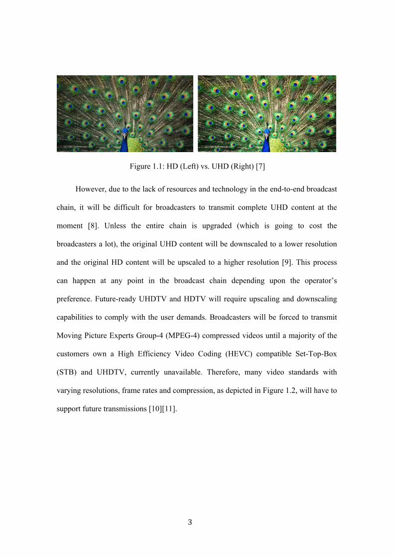
3
Figure 1.1: HD (Left) vs. UHD (Right) [7]
However, due to the lack of resources and technology in the end-to-end broadcast
chain, it will be difficult for broadcasters to transmit complete UHD content at the
moment [8]. Unless the entire chain is upgraded (which is going to cost the
broadcasters a lot), the original UHD content will be downscaled to a lower resolution
and the original HD content will be upscaled to a higher resolution [9]. This process
can happen at any point in the broadcast chain depending upon the operator’s
preference. Future-ready UHDTV and HDTV will require upscaling and downscaling
capabilities to comply with the user demands. Broadcasters will be forced to transmit
Moving Picture Experts Group-4 (MPEG-4) compressed videos until a majority of the
customers own a High Efficiency Video Coding (HEVC) compatible Set-Top-Box
(STB) and UHDTV, currently unavailable. Therefore, many video standards with
varying resolutions, frame rates and compression, as depicted in Figure 1.2, will have to
support future transmissions [10][11].
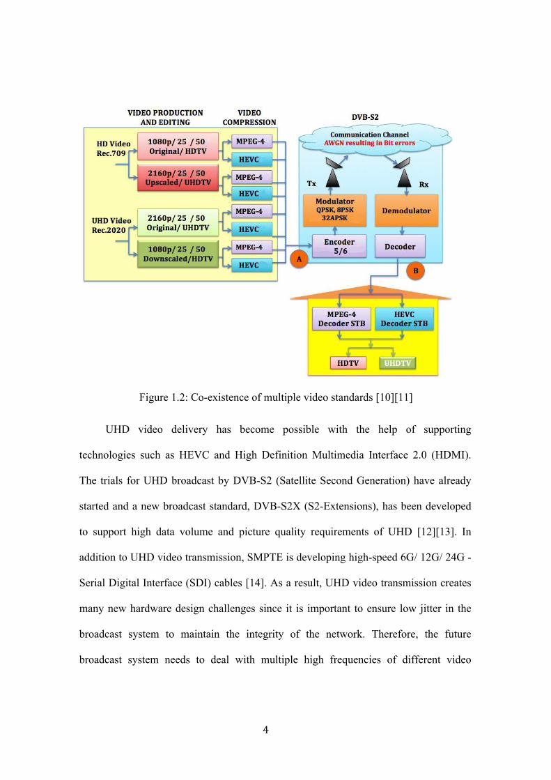
4
Figure 1.2: Co-existence of multiple video standards [10][11]
UHD video delivery has become possible with the help of supporting
technologies such as HEVC and High Definition Multimedia Interface 2.0 (HDMI).
The trials for UHD broadcast by DVB-S2 (Satellite Second Generation) have already
started and a new broadcast standard, DVB-S2X (S2-Extensions), has been developed
to support high data volume and picture quality requirements of UHD [12][13]. In
addition to UHD video transmission, SMPTE is developing high-speed 6G/ 12G/ 24G -
Serial Digital Interface (SDI) cables [14]. As a result, UHD video transmission creates
many new hardware design challenges since it is important to ensure low jitter in the
broadcast system to maintain the integrity of the network. Therefore, the future
broadcast system needs to deal with multiple high frequencies of different video
5
standards and since, a digital wireless communication is prone to noise or bit errors, it
is crucial to study the end-to-end signal performance of different video standards being
transmitted over-the-air. Bit Error Rate (BER) v/s Signal to Noise Ratio (SNR)
simulations provides an ideal way to determine the effects on the quality of signal
transmission [15].
While research work on UHD video quality assessment like Peak-SNR (PSNR)
calculation has been carried out and, subjective and objective assessments have become
quite common [16], there are very few research papers calculating the effect of noise on
UHD and HD videos with varying parameters, in a wireless transmission. The video
quality assessment is done mostly at the production level before video transmission is
done. Once the signal is transmitted over air, the video quality is bound to deteriorate
and hence, the study of noise channels on different types of videos is equally important.
Unlike many other forms of analysis, BER v/s SNR determines the full end-to-end
performance of a system at the given signal power, including the transmitter, receiver
and the medium between the two. By calculating BER, the bit errors caused by
disturbance on the transmission path can be corrected by using error correction methods
at the receiver [17].
1.3 Scope
In this research project,
• Signal performance (BER v/s SNR) of a UHD video transmission by DVB-S2,
will be observed and characterized by varying the codec (video compression
method), resolution and frame rate, in the presence of different kinds of

6
interferences, for different modulation and coding schemes.
• Interference experienced by the transmitted video signal, in a wireless
communication channel of DVB-S2, deteriorates the signal quality and thus, a
method to improve the signal recovery is also proposed.
The impact of signal performance is observed for the following:
• Shannon Channel Capacity
• Spectral Efficiency
• Coverage area: Distance between Transmitter and Receiver
• Service Area Separation Distance
• An adaptive video quality system using the proposed and developed
Principle of Inclusion
• Transmission Cost
This study is significant for broadcasters since the choice from varying
performance options is linked to the way broadcast will be delivered [18]. For example,
HD video should be aired at its standard resolution of 1080p (‘p’ means progressive
mode or full scanning), after being compressed by MPEG-4 video compression format;
however, to avoid investing on upgraded infrastructure, some broadcasters still transmit
it at 720p or 1080i (‘i’ means interlacing or half scanning) with MPEG-2 (old video
compression format, recommended for SD). UHD has an advanced feature of a faster
frame rate of 50fps and 100fps in progressive mode, however, in the initial phase of
UHD broadcast, the content might have to be broadcasted in interlaced form or 25fps

7
and users have to rely on expensive television sets to artificially generate frames by
software algorithms, which will still have inevitable artifacts [19]. This quality cannot
be assumed to be equivalent to an original video of 50fps in progressive mode.
Similarly, it is most likely for broadcasters to transmit UHD content using MPEG-4
(recommended for HD) video compression, instead of HEVC (latest video compression
format, recommended for UHD), and at 1080p resolution, instead of 2160p. Some
might just upscale the HD video to view them on UHDTV due to the lack of content or
downscale UHD videos to view them on HDTV due to the lack of infrastructure [20].
This dilemma of broadcasters and consumers has prevented the complete roll-out
of the real HDTV till now, and the same reason might prevent the complete roll-out of
the real UHDTV. Therefore, it is entirely the broadcaster’s decision, which video
compression and MODCOD (modulation-coding) scheme will be adopted for
transmitting a UHD video. There is a trade off between quality and cost in every option,
and this research will explore every aspect of these scenarios from which the
broadcasters can take an optimum decision towards their future planning of a UHD-
DVB broadcast profile [4][5]. Other than movies and TV programs, UHD video
broadcast will be useful in other applications where minute pixel data plays an
important role [21], applications include the following:
• Medical imaging
• Weather forecasting
• Disaster Recovery
• Education and security

8
1.4 Research Objective and Contribution
The objective of this research work is to define the requirement of a UHD
broadcast profile and contribute towards its standardization [22]. The investigation will
help members of EBU, SMPTE, DVB and ITU-R, to make strategic decisions for
future production and distribution technologies, by identifying the market demand per
service type, commercial requirements and the backward compatibility of the UHD
content with HDTV applications.
At the moment, many of the technical aspects of UHD broadcasting are yet to be
agreed upon at a global level. To make UHD broadcasting a reality, we need a complete
ecosystem, with content being made that the public wants, transmitters, receivers, and
displays that are readily available. The specification should also consider features that
the system would need to make it commercially successful. Some DVB Members think
that displays for UHD-2 are too far away to be considered now, while others argue that
UHD-2 is inevitable [23]. Therefore, we need to understand the requirements based on
the trends of UHD-1 and when we can expect UHD-2 on the market. We also need to
consider whether we can use DVB-S2 for UHD or not. Therefore, this research will
analyze the performance of UHD video signals, with varying parameters as compared
to HD, when transmitted by DVB-S2.
To analyze the UHD video performance in the future broadcast scenario, we first
need to understand the existing scenario. Hence, we need to study the performance of
HD and compare it with UHD. HD should only be viewed at a resolution of 1920x1080
pixels in 25fps progressive mode, and ideally on a TV screen above 42ʹʹ. However, not

9
many consumers will buy an expensive television of 42ʹʹ and not every broadcaster will
have enough bandwidth, to air every channel in full resolution, thereby, resulting in
non-ideal standard adoption. UHD has many parameters defining its video quality and
the broadcaster needs to decide, which set of parameter they need to choose for a
particular program and channel [24].
A news channel, where the anchor is mostly sitting in one place, talking to others,
is a low bandwidth broadcasting requirement. While, a sports channel showing F1 race,
where video graphics change every second, requires a higher frame rate and higher
bandwidth. This thesis contributes towards a detailed study of the parameters in every
combination of a UHD channel, which will help the broadcasters in the migration phase
from HD to UHD, as explained in the following tables:
Table 1.1: Contribution Towards Modulation and Coding Scheme What is
known [25] DVB-S2 Modulation and coding schemes
Fact [26] UHD content will be transmitted over the air, along with HD simulcasting. Hence, a detailed signal performance comparison between HD and UHD is required.
What is not known
Are UHD and HD videos going to perform similarly under every MODCOD scheme and Noise?
Thesis Contribution
Proposed experiments to determine whether:
1) UHD BER is higher or lower than HD in QPSK and 8PSK, 3/4 and 5/6 scheme, in the presence of AWGN
2) UHD BER is higher or lower than HD in QPSK and 16APSK, 3/4 and 5/6, in a Rician Fading Channel (K=5).
3) For all other cases, the BER of UHD and HD are almost the same
10
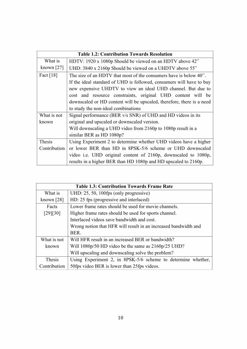
Table 1.2: Contribution Towards Resolution What is
known [27] HDTV: 1920 x 1080p Should be viewed on an HDTV above 42ʹʹ UHD: 3840 x 2160p Should be viewed on a UHDTV above 55ʹʹ
Fact [18] The size of an HDTV that most of the consumers have is below 40ʹʹ. If the ideal standard of UHD is followed, consumers will have to buy new expensive UHDTV to view an ideal UHD channel. But due to cost and resource constraints, original UHD content will be downscaled or HD content will be upscaled, therefore, there is a need to study the non-ideal combinations
What is not known
Signal performance (BER v/s SNR) of UHD and HD videos in its original and upscaled or downscaled version. Will downscaling a UHD video from 2160p to 1080p result in a similar BER as HD 1080p?
Thesis Contribution
Using Experiment 2 to determine whether UHD videos have a higher or lower BER than HD in 8PSK-5/6 scheme or UHD downscaled video i.e. UHD original content of 2160p, downscaled to 1080p, results in a higher BER than HD 1080p and HD upscaled to 2160p.
Table 1.3: Contribution Towards Frame Rate What is
known [28] UHD: 25, 50, 100fps (only progressive) HD: 25 fps (progressive and interlaced)
Facts [29][30]
Lower frame rates should be used for movie channels. Higher frame rates should be used for sports channel. Interlaced videos save bandwidth and cost. Wrong notion that HFR will result in an increased bandwidth and BER.
What is not known
Will HFR result in an increased BER or bandwidth? Will 1080p/50 HD video be the same as 2160p/25 UHD? Will upscaling and downscaling solve the problem?
Thesis Contribution
Using Experiment 2, in 8PSK-5/6 scheme to determine whether, 50fps video BER is lower than 25fps videos.

11
Table 1.4: Contribution Towards Video Compression What is known
[31][32]
MPEG-4: Currently being used for HD HEVC: 50% more efficient than MPEG-4 and is to be used for UHD
Facts [33]
HEVC is still being improved and its compatible hardware is still not widely available. Therefore, in the initial UHD broadcast phase, MPEG-4 will be used for UHD compression. If broadcasters use HEVC for UHD video compression, consumers cannot view UHD on their HDTVs. If broadcasters use MPEG-4, it will consume high bandwidth as one UHD channel will consume the bandwidth of four HD channels.
What is not known
Will MPEG-4 and HEVC compressed video, result in the same BER?
Thesis Contribution
Using Experiment 2, in 8PSK-5/6 to determine whether, HEVC compressed BER is lower than MPEG-4 due to a lower bit rate resulting in a lower BER. Observe HD and UHD and hence, determine if HEVC compression should be adopted for HD.

12
1.5 List of Publications
A number of peer-reviewed publications have been generated from the research
accomplished in this thesis.
• 1) Horace King, Urvashi Pal, “A Statistical Approach to Determine Handover
Success Using the Principle of Inclusion and Load Variation on Links in Wireless
Networks”, International Journal of Information, Communication Technology and
Applications (IJICTA), Vol. 1, No. 1 (2015), pp. 143-151, December 2015.
• 2) Urvashi Pal, Horace King, “Bit Error Rate (BER) analysis of UHD High
Frame Rate (HFR) videos through different modulation schemes”, International
Broadcasting Convention (IBC) - 2015, Future Zone, RAI Amsterdam, September
2015.
• 3) Urvashi Pal, Horace King, “Effect of Ultra High Definition (UHD) High
Frame Rates (HFR) on Video Transmission”, Society of Motion Pictures and
Television Engineers, Sydney (SMPTE), Australia, July 2015.
• 4) Urvashi pal, Horace King, “Effect of Modulation Scheme on Ultra-High
Definition (UHD) Video Transmission”, accepted for IEEE Wireless
Telecommunication symposium (WTS), New York City, USA, April 2015.
• 5) Urvashi Pal, Horace King, “DVB-S2 Channel Estimation and Decoding in
The Presence of Phase Noise for Non-Linear Channels”, International Journal of
Information, Communication Technology and Applications (IJICTA), Vol. 1, No. 1
(2015), pp. 112-127, March 2015.

13
1.6 Thesis Organization
This research is devoted to the standardization of UHD video transmission by
DVB-S2. Chapter 1 lays the foundation by analyzing the background literature,
establish the problem statement and provide the research objectives and contributions.
Chapter 2 analyzes UHD ecosystem and discusses the features added to the UHD
ecosystem such as 4K resolution, Higher Frame Rate, Wide Colour Gamut, Higher
Dynamic Range and the new advanced and highly efficient video codec HEVC. It also
discusses the different methods to broadcast this enormous video content. Further, it
describes the infrastructure required for UHD delivery through DVB-S2. In addition.
the latest television receivers available on the market today are discussed. The chapter is
summarized by setting the UHD roadmap of the future.
Chapter 3 analyzes and explains Encoding-Modulation and Decoding-
Demodulation in the DVB-S2 system. It also reviews effects on a signal in a wireless
communication channel due to Rician Fading, correlated phase noise and AWGN.
Chapter 4 analyzes the scenario of UHD video broadcasting through DVB-S2.
Since many organizations are working towards the standardization of DVB-UHD
standard, the problem of BER in this scenario is explored. The Importance of BER vs.
SNR calculation is explained and a method to reduce the error rate, known as Channel
Estimation using pilot bits, is proposed.
Chapter 5 proposes video performance evaluation method to calculate BER vs.
SNR graphs using MATLAB simulations. The scenario of multiple video standards in
the future is considered and video quality assessment is done. Following that, three

14
experiments are performed. In Experiment 1, two videos (HEVC HD 1080p/25 and
HEVC UHD 2160p/25) and transmitted through DVB-S2 model in the presence of
AWGN for different modulation schemes and code rates (QPSK, 8PSK, 16APSK and
32APSK & 3/4, 5/6 and 9/10 rate). In Experiment 2, sixteen different videos varying in
original content (HD, UHD) resolution (1080p, 2160p), frame rate (25fps, 50fps), codec
(MPEG-4, HEVC) are transmitted through DVB-S2 model in the presence of AWGN
only, for 8PSK-5/6 scheme. In Experiment 3, two videos of Experiment 1 are
transmitted through DVB-S2 in the presence of Rayleigh Fading Channel (K=0) and
Rician Fading Channel (K=5), correlated phase noise and AWGN. The same
experiment is repeated after applying channel estimation method using pilot bits, to
reduce the BER.
In Chapter 6, results of chapter 5 are used to calculate the Channel Capacity,
Coverage area (Distance between Transmitter and Receiver), Service area Separation
Distance. Using these parameters, the Principle of Inclusion is developed and
implemented and, a UHD parameter adaptive scenario is explained. It is shown that
there is an increase in the cost of transmission power to broadcast a UHD video, as
compared to HD using the developed formulations.
This thesis is concluded with a summary and future work possibilities in Chapter 7.

15
Chapter 2
Literature Review of UHD Ecosystem
2.1 Introduction
“The colours are breathtaking.
The clarity is flawless.
The definition is so sharp that viewers feel truly immersed in the action.” [19]
With a wealth of benefits including four times higher resolution than HD, faster
frame rate, higher dynamic range and a wider colour gamut, television and media
industry is on the cusp of a revolutionary transformation in video transmission. UHD’s
advanced technology promises to surpass consumer’s expectations. By region, its
household penetration will reach 33% in North America, 22% in Western Europe and
18% in Asia Pacific by 2020 [19]. Hence, the following features have been introduced
or modified to provide users with an ‘Ultra’-HD experience.
2.2 Video Production
2.2.1 4K Resolution
The human vision is one of the most complex parts of the human body. The eye
perceives movement, senses depth, and sees a range of colours greater than any current
existing video technology is able to display. UHDTV has a resolution of 3840 x 2160
pixels, which is four times the resolution of HDTV. This means that there is four times
more information displayed on screen, which is one of the factors to enhance the video
16
quality. The ideal size of a UHDTV is supposed to be around 55ʺ to 80ʺ. Based on the
size of television, viewing distance is calculated to maintain the maximum perceived
angular resolution because there are limits to what an eye can perceive [34]. If you sit
too close to the TV, you will be seeing the unwanted individual pixels and if you sit too
far, you won't be able to observe all the details in the video. That means, if you sit too
far away from a UHDTV, the UHD content will look like HD. As a result, the viewing
distance for a UHDTV is half of what is required for HDTV.
2.2.2 High Frame Rates (HFR)
Ultra HD changes the way moving images are displayed, stored, and transmitted.
To ensure a smooth viewing experience, HFRs will be used for UHD and HD videos in
the future [2]. Until now, interlaced scanning (odd and even lines transmitted in turn)
was being used to save bandwidth. However, there was a trade off with quality.
Although, most recent HDTVs have the technology to de-interlace the frames, the
artifacts could never be eliminated completely. Hence for UHD, the signal will mostly
be transmitted in progressive mode, since it offers higher vertical resolution, better
picture quality and easier frame conversion to other formats.
Frame rate used till now is 25fps for HD but for UHD, we will be dealing with
50fps, 100fps or even higher. Increasing the frame rate increases the smoothness of a
video, especially for high motion contents [35]. Increased information per second of the
video with more frames enhances the smoothness and colour rendition.
17
HFR technology was first introduced for 3D movies and has now been adopted
for UHD videos [35]. “The Hobbit: An unexpected journey” (2012) in 3D, was the first
movie to be shot at an HFR of 48fps (double of 24fps). Simultaneously, a new frame
rate for HDTV at 50 fps (progressive) has also been standardized, keeping in mind that
UHDTV will take time to penetrate the market and there is already a demand for
increased video quality among the users [6]. DVB has included 1080p/50 format in its
DVB specification TS 101 154 V1.9.1, for Advanced Video Coding (AVC) and
Scalable Video Coding (SVC). Broadcasting in 1080/50p will be possible when new
UHD STB arrive in the market (with HEVC encoding), offering progressive mode in
the channels, not yet available.
2.2.3 Wide Colour Gamut (WCG)
UHD technology allows for a greater array of colours to be perceived by viewers.
Rec.709 gives HD’s colour space, while for UHD, Rec.2020 has been standardized, as
shown in Figure 2.1. Rec.709 covers 1.6 million colours while Rec.2020 covers 1
billion. In other words, Rec.709 captures 35% of the natural view, while Rec.2020
captures 75%. Hence, watching a UHD video will be similar to watching a 3D video
without the glasses. Rendering a particular colour in a pixel is given by a video’s colour
depth or bit depth, as it is the number of bits required to define the colour of a pixel.
UHD includes a richer colour depth of 10-bit or 12-bit as compared to 8-bit used by
HD. 8-bit consists of (8 x 8 x 8) values, ranging from 0 - 255 colours for RGB, while
10-bit consists of (10 x 10 x 10) values, each ranging from 0 - 1023 colours. The wide
range of colours is going to radically enhance the picture quality of a UHD video. This

18
improvement in display technology will enable the human eye to use more of its
potential and foster viewing experience that will appear more and more lifelike [36].
Figure 2.1: HD and UHD Colour Space [37]
2.2.4 High Dynamic Range (HDR)
One more feature that will improve the video quality, is allowing a High Dynamic
Range (HDR) that will help produce a greater dynamic range of luminosity [38]. With
current technology, details in the dark are often not easily perceptible and important
information displayed onscreen can be lost. With HDR, these details will be displayed
more clearly, even when there is unfavorable lighting. As HDR technology adds greater
depth and detail at both ends of the light level spectrum, it has been shown to create an
increase in subjective quality for viewers, regardless of screen size and viewing distance
[39][40].

19
2.3 Video Compression: MPEG-4 vs. HEVC
At present, MPEG-4 video compression format is being used to watch HD
channels on our HDTVs. HEVC is the new video compression method, developed
especially to compress the huge data of UHD and has been adopted for its transmission
by DVB [41].
2.3.1 Advantages of HEVC compared to MPEG-4 [42][43]:
• HEVC offers 50% higher video compression and quality as compared to MPEG-4
and therefore, will make the transmission of UHD content more efficient by saving
the bandwidth significantly. Example: Using MPEG-4, 1 UHD channel will be
available, and using HEVC, 4 UHD channels will be available using the same
bandwidth.
• With the high performance of HEVC, about the same bit-rate used for 1080i/50
broadcast will be required for 1080p/50, and a better image quality will be delivered
to the home. This is because compression avoids transmitting the entire frame
whose information has already been transmitted in the previous frames. It only
transmits the residual information between the referenced frame and current frame.
Hence, the total bit rate is reduced and bandwidth is saved [15].
2.3.2 Disadvantages of HEVC compared to MPEG-4 [42][43]:
• HEVC encoder and decoder is at its early stage of development and not much has
been finalized yet.
• To use HEVC, broadcasters will have to invest in upgraded infrastructure, which
will take time and cost a lot of money.

20
• If the broadcasters start using HEVC to transmit UHD, consumers will be forced to
dump their existing HDTVs and buy expensive HEVC compatible UHDTVs, and
this will take time.
• UHD HEVC channels TV package will be costlier than what the consumer is paying
at present for HD MPEG-4 channels, hence, HEVC-UHD will take time to
successfully hit the market.
Due to the disadvantages of HEVC, in the early migration phase of UHD the
broadcasters will be left with no other choice, but to broadcast UHD channels in
MPEG-4 format, compromising quality and bandwidth. HEVC was previously being
developed for only-progressive mode, however, most of the producers and broadcasters
still use the legacy interlaced format and cannot be abandoned at once and migrated to
progressive format so soon; leading to HEVC introducing interlaced video compression.
The introduction of new video formats (1080p/50, 2160p/ 25, 2160p/50) in addition to
an existing one (720p or 1080i) may require simulcasting the same service at different
formats. In such a scenario, the combination of MPEG-4 or AVC, SVC and HEVC will
be used for different video formats [10][44].
HEVC Working:
HEVC video codec divides a frame into Coding Tree Units (CTU), which consist
of Coding Tree Blocks (CTB) i.e. one Luma (Y), two Chroma samples (Cb, Cr) and
associated syntax elements [42]. Each CTB is of the same size as a CTU. These CTBs
are further split up into variable Coding Blocks (CB) for inter-picture or intra-picture
prediction. HEVC handles Coding Blocks of length (64 x 64), (32 x 32), (16x16) and

21
(8 x 8) pixels, by changing the size according to texture (MPEG-4 uses macro-block
sizes maximum of (16 x 16) pixels). Different Prediction Blocks (PB) are introduced for
precise prediction of the moving images. A Coding Block (CB) is further split into
Transform Blocks (TB) to code the difference between the predicted image and the
actual image. The complete process is explained in Figure 2.2. Figure 2.3 shows a
comparison of HEVC and MPEG-4 compression technique [42].
Step 1:
CTU CTU CTU CTU CTU CTU CTU CTU CTU CTU CTU CTU CTU CTU CTU CTU CTU CTU CTU CTU
Image Frame Divided into CTUs
Figure 2.2: HEVC Compression Technique [31]
Figure 2.3: Comparison of MPEG-4/H.264 and HEVC/H.265 Compression [45]

22
2.4 Video Broadcasting
2.4.1 Using DVB-S2/S2X
DVB-S2 is the technique for Direct-to-Home (DTH) services. It uses Bose-
Chaudhuri-Hocquenghem (BCH) + Low Density Parity Check (LDPC) encoder-
decoder and interleaver (except for QPSK), combined with a variety of modulation
schemes and code rates, along with Adaptive Coding Modulation (ACM), resulting in
an improved efficiency of 30-35% as compared to DVB-S [46]. The adoption of new S2
Extension (S2X) will further improve the efficiency by 20% (for DTH) and 51% for
other professional applications, by providing more speed, mobility and robustness.
DVB-S2X target is to support the rising demand for higher quality images with the rise
of UHDTV and HEVC [47].
New features of S2 Extensions include bonding of TV streams (Channel Bonding)
for DTH by sending one big Transport Stream (TS) over many transponders at the same
time and merging their spare capacities. Stat-mux provides only 12% gain, therefore,
more channels cannot be added, however, by using Channel bonding, 12% extra gain is
achievable. More modulation schemes have been adopted for S2X, such as 64, 128 and
256 APSK and more Forward Error Correction (FEC) code rates have been added for
each modulation scheme, as given in Table 2.1. Hence, ACM provides full efficiency,
closer to the theoretical Shannon Limit, as compared to DVB-S2. Very low SNR
Modulation-Coding rates (MODCODs) for BPSK and QPSK to support small antenna
mobile (land, sea, air) applications are also added. More granularity with low roll offs

23
(5%, 10% and 15%), wideband implementation, and additional scrambling sequences
are added, resulting in an increased bandwidth [48].
Table 2.1: Code rates comparison between DVB-S2 and DVB-S2X [46][14]
DVB-S2 DVB-S2X QPSK 1/2, 1/4, 1/3, 2/5, 3/5, 2/3,
3/4, 4/5, 5/6, 8/9, 9/10 13/45, 9/20, 11/20
8PSK 3/5, 2/3, 3/4, 5/6, 8/9, 9/10 23/36, 25/36, 13/18 16APSK 2/3, 3/4, 4/5, 5/6, 8/9, 9/10 26/45, 3/5, 28/45, 23/36,25/36, 13/18, 7/9, 77/90 32APSK 3/4, 4/5, 5/6, 8/9, 9/10 32/45, 11/15, 7/9
2.4.2 Using Other Methods
2.4.2.1 DVB-T2/T2-Lite
Digital Video Broadcasting through Terrestrial Network Second Generation
(DVB-T2) has been primarily designed for fixed reception; however, in recent years
there has been a noteworthy growth in the demand for wireless communication [2]. Its
advanced version has recently been standardized i.e. DVB-T2-Lite for mobile and
portable reception to reduce implementation costs. This technology uses a combination
of satellite transmission link for long distance communication and terrestrial network
link to reach the end user. It uses the concept of Single Frequency Network (SFN) and
Orthogonal Frequency Division Multiplexing (OFDM) and involves LDPC encoders
with Multiple Physical Layer Pipes (PLP) for different applications [49][50]. This
mechanism allows T2-Lite and T2-base to be transmitted in one RF channel, even when
the two profiles use different Fast Fourier Transform (FFT) sizes or guard intervals. The
PLP transmission parameters for the mobile service are compliant to the T2-Lite

24
parameter set. However, the disadvantage of this technology is that it is not possible to
broadcast throughout the year due to adverse weather conditions and the available
bandwidth is also low, as compared to DVB-S2. DVB-T2 system model, given in
Figure 2.4 [49].
Figure 2.4: DVB-T2 System Architecture [49]
2.4.2.2 IPTV: HbbTV and MPEG-DASH
Another technology supporting 4K video delivery through Internet Protocol-TV (IPTV)
has recently been standardized and involves MPEG-Dynamic Adaptive Streaming Over
HTTP (DASH) and Hybrid Television (HbbTV) [51]. MPEG-DASH is the protocol that
allows a smooth conversion of various video formats on the Internet. It also has an
adaptive bit rate technology to adjust the video parameters (resolution, frame rate, etc.)
as per the available bandwidth [52]. Other features on which the industry is working on
are for improving the buffer speed, cache management and video-parameter transition
25
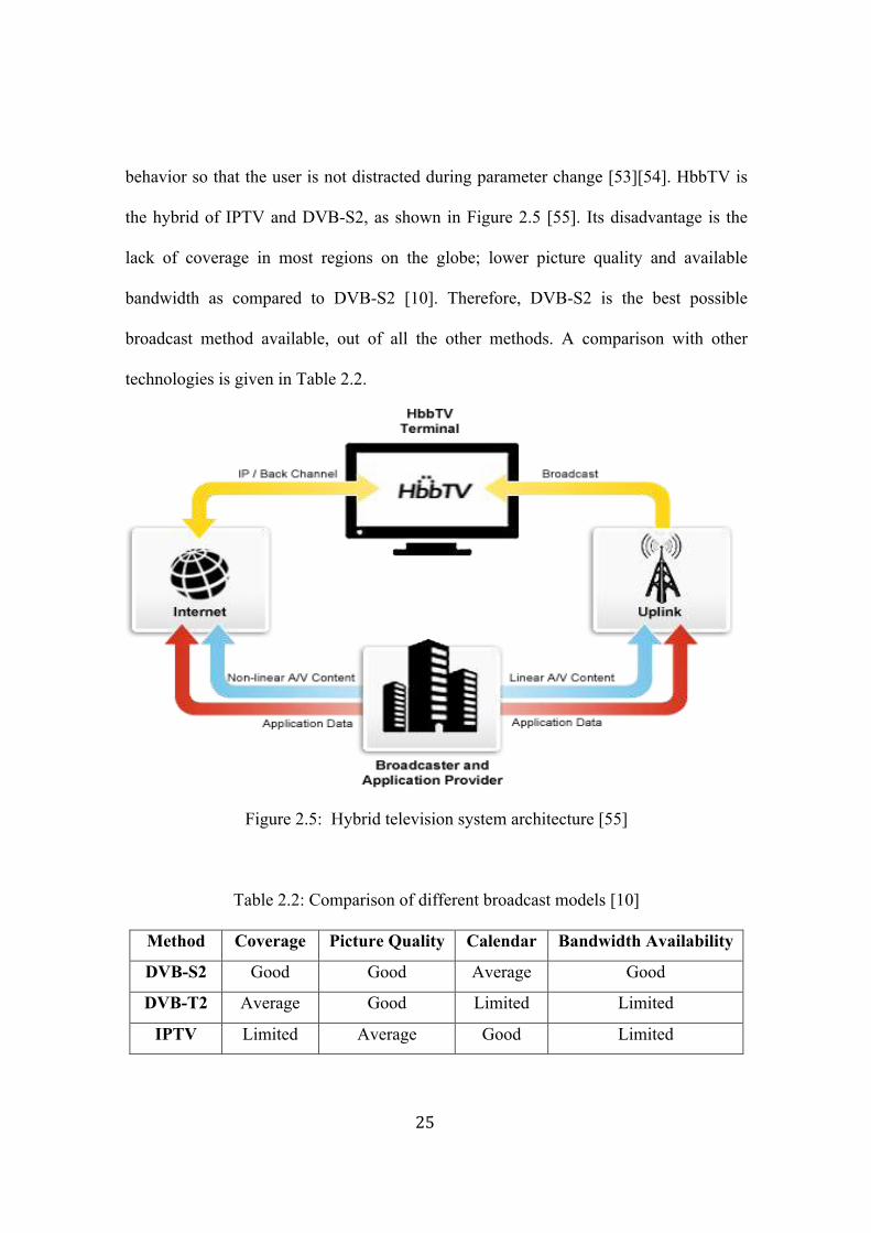
behavior so that the user is not distracted during parameter change [53][54]. HbbTV is
the hybrid of IPTV and DVB-S2, as shown in Figure 2.5 [55]. Its disadvantage is the
lack of coverage in most regions on the globe; lower picture quality and available
bandwidth as compared to DVB-S2 [10]. Therefore, DVB-S2 is the best possible
broadcast method available, out of all the other methods. A comparison with other
technologies is given in Table 2.2.
Figure 2.5: Hybrid television system architecture [55]
Table 2.2: Comparison of different broadcast models [10]
Method Coverage Picture Quality Calendar Bandwidth Availability
DVB-S2 Good Good Average Good
DVB-T2 Average Good Limited Limited
IPTV Limited Average Good Limited

26
2.5 Video Delivery Mechanisms
2.5.1 DVB-S2 UHD Satellites
At the present time, UHDTV channels are being trialed and tested with the help of
demo channels via DVB-S2 supported satellites, which are inline with the DVB-
UHDTV phase-1 specifications [56]. Table 2.3. describes the technical parameters for
satellite reception of a UHDTV channel by DVB-S2 satellites.
Table 2.3: Technical parameters for satellite reception of a UHD channel [57][58]
UHD Satellite Frequency (MHz) Modulation-Coding
Hot Bird 4K1, 13°East Eutelsat 10A, 10°East Eutelsat 10A, 10°East SES Astra, 19.2°East
11296 11429 11346 10994
8PSK, 3/4 8PSK, 5/6 8PSK, 5/6 8PSK, 5/6
2.5.2 Serial Digital Interface (SDI) Cables and STBs
Table 2.4 enlists current and future SDI cables standardized for supporting
UHDTV. Due to the high demand for UHD video standard, video equipment suppliers
are already working on future technologies to support faster data rates.
Table 2.4: SMPTE SDI cables supporting PAL videos [14][15]
Cable Supported Video upto Data rate
SD-SDI HD-SDI 3G-SDI 6G-SDI 12-SDI 24-SDI
480i/25 270p/50, 1080i/50
1080p/50 2160p/25 (upcoming) 2160p/50 (unofficial)
Next-gen tech (unofficial)
270 Mbps 1.585 Gbps 2.97 Gbps 5.97 Gbps 11.8 Gbps 23.xx Gbps

27
From Table 2.4, it is evident that future SDI cables take into account the increase in the
number of pixels and frame rates and in concert with the increase in data rates into
higher Gbps.
2.5.3 High Definition Multimedia Interface (HDMI)
HDMI 2.0 can transmit 12-bit per sample RGB at 2160p (progressive) and
24/25/30 fps or it can transmit 12-bits per sample 4:2:2/4:2:0 YCbCr at 2160p and 50/60
fps. UHDTVs released before HDMI 2.0, support the current HDMI 1.4 version, which
limits UHD content to 24-30 fps [59]. Even after the launch of 6G-SDI cables, viewers
will only be able to receive UHD channels on their television sets, if they have a
compatible 4K STB supporting the latest HDMI 2.0 standard.
Till now, most of the TVs and STBs use HDMI 1.4a (6.05 Gbps usable
bandwidth), which supports videos for 1080p/60 (1920 x 1080 resolution, 60 frames per
second in progressive mode) and 2160p/30. However, to support 2160p/60 and other
enhanced features of UHD video and audio, we need HDMI 2.0 (14.4 usable bandwidth
out of 18 Gbps), This upgrade can either be a firmware update or a hardware update
depending on different TV and STB manufacturers [60]. Table 2.5 highlights its
features.
Table 2.5: HDMI 1.4a vs. HDMI 2.0 [59]
Format/ HDMI version
1080p/ 25fps
1080p/ 50fps
2160p/ 25fps
2160p/ 50fps
8-bit 10-bit 12-bit
4:4:4 Sampling
1.4a Yes Yes Yes NO Yes NO NO
2.0 Yes Yes Yes Yes Yes Yes Yes

28
2.6 Display and Backlight Technology
The colour accuracy of a Liquid Crystal Display (LCD) TV screen depends on the
backlight technology used to produce the white light. The various backlight
technologies available today are:
Cold-Cathode Fluorescent Lamps (CCFL) is the old backlight technology that
produces light strongest in greens and not exactly white and therefore, are not suitable
for UHDTVs.
Light Emitting Diodes (LED) backlight with LCD display is the perfect choice
for UHDTV as they produce whiter whites than CCFL since they use a non-coloured
light source to illuminate the screen.
Quantum Dots (QD) is the same LED backlight technology for LCD display;
however, the method to create colours is new. Quantum Dots directly convert light from
blue LEDs into primary colours, rather than using the existing white LEDs. A QD emits
light in a specific Gaussian distribution resulting in more accurate colours with
improved brightness, that are not colour filtered and thus require low power.
Organic Light-Emitting Diode (OLED) display is an alternative to LCD Thin
Film Transistor (TFT) display that offers higher brightness and contrast ratio since it is
a light emitter and creates Lambertian light. It can be seen uniformly at all angles and
gives a very pleasing effect. It does not require any backlight and can be made thinner
(at 2mm) than LED (3mm). OLEDs are expensive and require a glass-covered screen.
Curved and Flexible Displays can be for both, OLEDs and LCDs. This new
innovative display technology improves the image quality and readability by
29
eliminating the reflections from ambient lights sources. Curved displays are suitable for
TVs as well as for mobiles, as it allows the displays to run at lower brightness, thus,
increasing the power efficiency and battery running time.
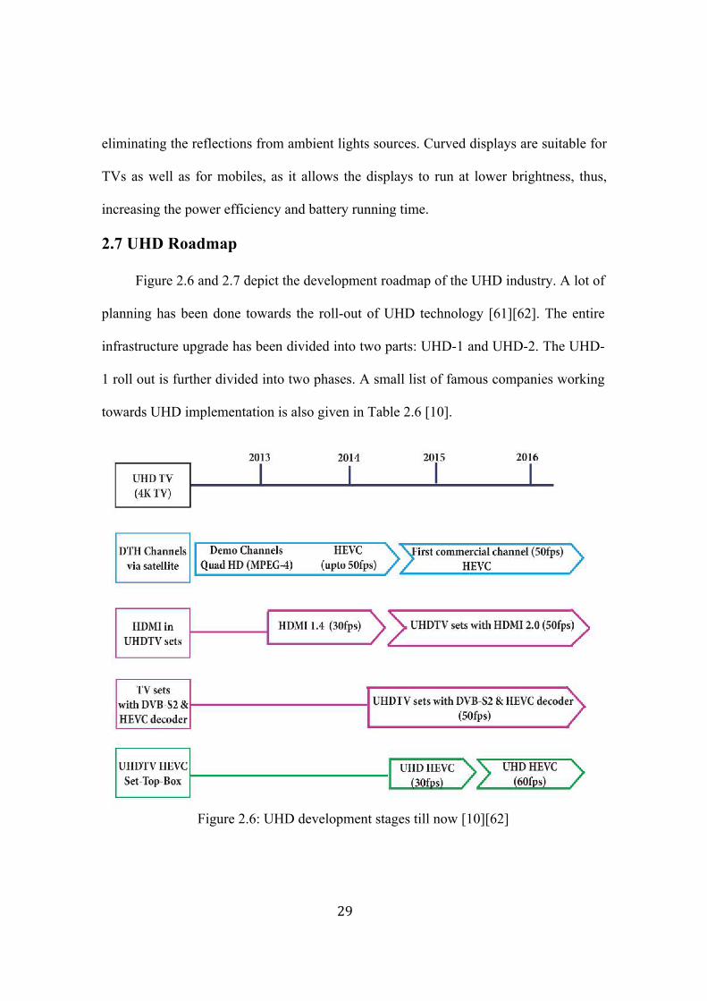
2.7 UHD Roadmap
Figure 2.6 and 2.7 depict the development roadmap of the UHD industry. A lot of
planning has been done towards the roll-out of UHD technology [61][62]. The entire
infrastructure upgrade has been divided into two parts: UHD-1 and UHD-2. The UHD-
1 roll out is further divided into two phases. A small list of famous companies working
towards UHD implementation is also given in Table 2.6 [10].
Figure 2.6: UHD development stages till now [10][62]

30
Table 2.6: List of some companies working towards UHD [10]
Professional 4K Cameras HEVC 4K-UHDTV
Blackmagic Design, Canon, Panasonic, Red Epic, Sony
ATEME, Elemental, Envivo, Ericsson, Harmonic, Rohde & Schwarz
Sony, Samsung, Panasonic, LG
Figure 2.7: UHD future roadmap [10][62]
2.8 Summary
In this chapter, a detailed analysis of Ultra-High-Definition video parameters and
requirements has been carried out. For a successful transmission and reception of a
UHD video, it is important that every block in the broadcast chain must be upgraded.
This will lead to an overall increase in the cost of production and broadcasting but the
enhanced video quality with richer colours and dynamic motion range makes the effort
totally worth it. Still, at the moment, the broadcasters will opt for a trade off in quality
by artificially upscaling a lower resolution content rather than using the original high
resolution content in the initial phase of broadcasting [63]. The availability of numerous
options to select from for a UHD video will itself create confusion in the future
broadcast scenario for the DTH operators. It is important that advanced hardwares
support interoperability at every stage, which will take time, is supported and enhanced
as the technology advances.

31
Chapter 3
Performance Analysis of DVB-S2
3.1 Introduction
Digital Video Broadcast-Satellite Second Generation (DVB-S2) is an audio and
video broadcast standard for DTH, HDTV and MPEG-4 related services in Fixed
Satellite Services (FSS) and Broadcast Satellite Services (BSS) bands. It is a successor
to DVB-S (first generation), and follows a QPSK modulation scheme and Forward
Error Correction (FEC), along with Reed–Solomon (RS) coding. For professional end-
to-end transmission of audio and video signals and Digital Satellite News Gathering
(DSNG), DVB proposed the next generation standard for video broadcasting i.e. DVB-
S2 [25].
DVB-S2 uses Low Density Parity Check (LDPC) coding, Variable Coding and
Modulation (VCM), and Adaptive Coding and Modulation (ACM) to minimize
bandwidth wastage. It uses QPSK, 8PSK, 16PSK, and 32APSK modulation schemes
along with various code rates and also supports backward compatibility. As a result of
these characteristic, the satellite transmission capacity increases by 30-35 % for a given
symbol rate and SNR as compared to DVB-S [46].
In a Pay-TV DTH system, video is recorded and sent to the relevant teleport and
TV studio, where post-production/editing is done. Here the video is processed in the
form of binary bits. It is then encrypted (encoded and modulated) and transmitted over
the air in the form of RF signals. DVB-S2 satellite receives it and downlinks it back to

32
the earth. The signal is received, converted back to digital and decrypted (decoded and
demodulated) by an STB of the particular broadcaster. The user can only view the
video after subscribing/paying to that broadcaster [63]. This procedure is depicted in
Figure 3.1 and its technical block schematic is given in Figure 3.2.
Figure 3.1: Direct-To-Home Pay-TV system model [10]
Figure 3.2: DVB-S2 block schematic [46]

33
3.2 Transmitter
It works on the message to deliver a suitable signal for transmission over the
communication channel. In 1982, Ungerbôeck released his landmark paper on Trellis
Coded Modulation (TCM), which states that Modulation and Coding together give an
improved performance and help to achieve a power and bandwidth efficient wireless
communication system. DVB-S2 transmitter consists of an LDPC encoder and a
modulator to achieve performance close to the channel capacity [64]. In this report,
study of an LDPC-coded modulation in the midst of Additive White Gaussian Noise
(AWGN), correlated phase noise and a Rician Fading Channel is done. For a
bandwidth-limited system, the higher the modulation scheme, the higher the spectral
efficiency. However, there is a trade off between bandwidth and the required signal
power. This is compromised with a loss of error performance.
3.2.1 Modulator Selection
3.2.1.1 Quadrature Phase Shift Keying (QPSK) Modulator
QPSK is a highly robust modulation scheme, as its states are far apart for the
receiver to detect and decode the channel properly, even in the presence of noise. The
normalized average energy per symbol shall be equal to one. Two bits are mapped to a
QPSK symbol i.e. bits 2i and 2i+1 determines the ith QPSK symbol, where i = 0, 1, 2,.,
(N/2)-1 and N is the coded LDPC block size. Gray coding is used to minimize the BER
by keeping the transition between two continuous bits equal to one bit. When this
property is followed, the receiver knows that the next code is different from the present
one by only one bit and this helps in a better decoding technique with low probability

34
of incorrect detection. However, its disadvantage is that its information rate per symbol
is very low i.e. only 2 bits per symbol, as shown in Figure 3.3 and it is sensitive to
phase variations, a phenomenon highly undesirable by DVB-S2.
3.2.1.2 8-Phase Shift Keying (8PSK) Modulator
This is the most commonly used modulation scheme for satellite video
broadcasting, other than QPSK, and transmits 8 symbols at a time and 3 bits per
symbol. This increases the efficiency of the system as compared to QPSK. However, its
hardware complexity is higher than QPSK and it requires high transmission power. Its
BER is also higher than QPSK. The bit-mapping diagram to achieve 8PSK
constellation is shown in Figure 3.3. The bit mapping uses gray coding for signal
recovery. The normalized average energy per symbol is equal to one. After the bits are
encoded and interleaved, the 3i, 3i+1 and 3i+2 bit of the interleaver output determine the
ith 8PSK symbol, where i = 0, 1, 2, ...(N/3)-1 and N is the coded LDPC block size.
Figure 3.3: Constellation Diagram of QPSK (left) and 8PSK (right) [25]

35
3.2.1.3 16-Amplitude Phase Shift Keying (16APSK) Modulator
The 16APSK modulation constellation, as shown in Figure 3.4, is composed of
two concentric rings of uniformly spaced 4 and 12 PSK points, respectively in the inner
ring of radius R1 and outer ring of radius R2. The ratio of the outer circle radius to the
inner circle radius (γ = R2 /R1) is given in Table 3.1. Two are the admitted values for
the constellation amplitudes, allowing performance optimization according to the
channel characteristics
• E=1 (E=unit average symbol energy) corresponding to [R1]2 + 3[R2]2 = 4
• R2 =1
which means that the normalized energy of the bits in each radius is equal to 1 and bits
4i, 4i+1, 4i+2 and 4i+3 of the interleaver output determine the ith 16APSK symbol, where
i = 0, 1, 2, …, (N/4)-1 and N is the coded LDPC block size.
Table 3.1: Optimum Constellation Radius Ratio for 16APSK [25]
Code Rate Efficiency γ 2/3 2,66 3,15 3/4 2,99 2,85 4/5 3,19 2,75 5/6 3,32 2,70 8/9 3,55 2,60
9/10 3,59 2,57 3.2.1.4 32-Amplitude Phase Shift Keying (32APSK) Modulator
32APSK has better spectral efficiency i.e. highest bits per symbol than QPSK and
8PSK. 32APSK points are optimized by placing them in concentric circles of constant
amplitude, with uniformly spaced 4,12, and 16 PSK points, respectively in R1
(innermost), R2 and R3, as shown in Figure 3.4, ensuring that the states in a particular
ring will react to distortion in the same manner. Signal compression does not

36
significantly change the spacing between the states (Euclidean distance), resulting in a
better signal recovery. However, 32APSK requires higher Carrier-to-Noise ratio and
pre-distortion methods (varying space between rings) before transmission, so that it
cancels the non-linear distortion experienced during transmission and this is done using
constellation amplitudes, γ1 and γ2, as explained in Table 3.2.
• E = 1 (E=unit average symbol energy)
• [R1]2 + 3[R2]2 + 4[R3]2 = 8
• R3 =1
Bits 5i, 5i+1, 5i+2, 5i+3 and 5i+4 of the interleaver output determine the ith 32APSK
symbol, where i = 0, 1, 2, (N/5)-1.
Table 3.2: Optimum Constellation Radius Ratios for 32APSK [25]
Code Rate Efficiency γ1 = R2/R1 γ2 = R3/R1 3/4 3,74 2,84 5,27 4/5 3,99 2,72 4,87 5/6 4,15 2,64 4,64 8/9 4,43 2,65 4,33
9/10 4,49 2,53 4,30
Figure 3.4: Constellation Diagram of 16APSK and 32APSK [25]

37
3.3 Analysis of The Transmission Channel
3.3.1 Rician Fading Channel
A channel acts as a medium for transmitting signal from the transmitter to the
receiver. The transmission path keeps varying as the Line Of Sight (LOS) keeps
changing according to the obstructions faced between the transmitter and receiver. In
addition to multipath reflection from obstructing objects, the transmission path of the
signal may increase. If the transmission path keeps increasing, the signal strength keeps
decreasing. For this reason, radio channel modeling has been the most difficult task in
communication systems. Therefore, modeling is done based on physical measurements
made on the intended communication system.
In a radio communication system, the instantaneous signal received keeps
fluctuating over time. This is because the received signal is the sum of many
contributions coming from different directions due to multipath. Therefore, the phase is
always varying with time. Two types of fading are considered here: Small Scale Fading
and Large Scale Fading. When there is a LOS between the transmitter and receiver, the
received signal is the sum of a complex exponential and a narrowband Gaussian
process, which are known as the LOS component and the diffuse component
respectively. The relative strength of the direct and scattered components of the
received signal is expressed by the Rician factor. The Rice Fading Distribution models
the variations in the signal envelope in a narrow-band multipath fading channel for a
direct LOS path between transmitter and receiver.

38
Suppose, gI(t) and gQ(t) are Gaussian random processes with non-zero means
mI(t) and mQ(t), respectively and b0 represents the variance of gI(t1) and gQ(t1) [65]. The
magnitude of the received complex envelope at time ‘t1’ has a Rician distribution as:
𝑓 𝑥 = !!!𝑒𝑥𝑝 − !!!!!
!!!𝐼!
!"!!
; x ≥ 0, (3.5)
𝑠! = 𝑚!! 𝑡 + 𝑚!
! (𝑡) (3.6)
where,
f(x): Received Signal Envelope
s2 = specular power (LOS component)
2b0 = scattered power (non-LOS component)
K is defined as the ratio of the specular power to scattered power, i.e.
𝐾 = !!
!!! (3.7)
Equation (3.7) can be rewritten in terms of Rice Factor and average envelope power
E[α2] = Ω = s2 + 2bo (3.8)
where, K and Ω are shape and scale parameters, respectively. Therefore,
𝑠! = !!!!!
(3.9)
2𝑏! = !!!!
(3.10)
Rice Probability Density function (PDF) of the received signal envelope is given by
𝑓 𝑥 = ! !!! !!
exp –𝐾 − !!! !!
! 𝐼! 2 ! !!! !
! (3.11)
Where:
Io: Oth-order modified Bessel function

39
‘K’ is described as the ratio of the power received via the LOS path to the power
contribution of the non-LOS paths, and is a measure of fading whose estimate is
important in link budget calculations. Therefore, for higher ‘K’ factor i.e. a better LOS,
the correlation is lower and signal performance is higher. Similarly, for low LOS, the
correlation between signal samples is higher and the estimator’s performance
deteriorates as the number of independent samples reduces. In this thesis, analysis is
done for various modulation schemes and code rates for different ‘K’ factors. ‘K = 0’ is
the case of Rayleigh Fading Channel where there is no LOS and ‘K > 0’ which is the
case of Rician Fading Channel. Higher ‘K’ is due to lower noise. The following
equation describes the magnitude of the received envelope for several values of ‘m’
(the Nakagami shape factor) by the distribution:
𝑓 𝑥 = !!!!!!!!
!(!)!!𝑒𝑥𝑝 −!"!
! 𝑚 ≥ !
! (3.12)
Where,
m = 1, the distribution becomes Rayleigh distribution
m = 1/2, it becomes a one-sided Gaussian distribution
m ! ∞, means no fading
𝐾 = !!!!!! !!!!
m > 1 (3.13)
m = (!!!)!
(!!!!) (3.14)

40
3.3.2 Phase Noise
The output signal of an oscillator will always have some unwanted noise, which is
basically spurious frequencies from the surroundings, harmonics and sub-harmonics
[66].
Ideal Signal: V(t) = A0 sin (2π f0 t) (3.15)
V(t): Variance
A0: nominal peak voltage
f0: nominal fundamental frequency
t: time
After adding Amplitude (AM) noise to (3.15):
V(t) = [A0 + e(t)] sin (2 πf0 t) (3.16)
e(t): Random deviation of amplitude from nominal “AM noise”
After adding random phase component to (3.16):
V(t) = [A0 + e(t)] sin [2 πf0 t + ∆ϕ(t)] (3.17)
∆ϕ(t): Random deviation of phase from nominal “phase noise”
At amplitude level, oscillators get saturated; therefore, AM noise can be neglected.
V(t) = A0 sin [2 πf0 t + ∆ϕ(t)] (3.18)
Now add a deterministic component to the phase in (3.18):
V(t) = A0 sin [2 πf0 t + ∆ϕ(t) + md sin (2 πfd t) ] (3.19)
md: Amplitude of deterministic signal, phase modulating the carrier
fd: Frequency of the deterministic signal
More detailed explanation is given in section 5.5.

41
3.3.3 Additive White Gaussian Noise (AWGN) Channel
Additive White Gaussian Noise (AWGN) is the channel in which noise is linearly
added in wideband and white noise with constant spectral density and a Gaussian
distribution of amplitude at the receiver [67].
Suppose,
Yi = Xi + Zi (3.20)
Where,
Yi = Channel Output
Xi = Channel Input
Zi = Zero-mean Gaussian with variance N: Zi ~ ℵ (0,N)
For an input codeword (x1, x2, ...., xn), the average power is constrained so that
!!
𝑥!!!!!! ≤ 𝑃 (3.21)
Suppose + √P or - √P is sent over the channel.
The receiver looks at the received signal amplitude and determines the signal
transmitted using a threshold test.
Therefore,
𝑃! = !!
𝑃 𝑌 < 0 𝑋 = + 𝑃 + !!𝑃 𝑌 > 0 𝑋 = − 𝑃 (3.22)
= 12𝑃 𝑍 < − 𝑃 𝑋 = + 𝑃 +
12𝑃(𝑍 > 𝑃|𝑋 = − 𝑃)
= 𝑃(𝑍 > 𝑃)
Normal Cumulative Probability Function = !!!"
!! 𝑒!!!/!!𝑑𝑥 (3.23)

42
Probability of error = 𝑄 !!
= 1−Φ !!
(3.24)
Where
𝑄 𝑥 = !!!
𝑒!!!/!𝑑𝑥!! (3.25)
Φ x = !!!
𝑒!!!/!𝑑𝑥!!! (3.26)
The information capacity of the Gaussian channel with power constraint is
𝐶 = max! ! :!!!!! 𝐼(𝑋;𝑌) (3.27)
A rate R is achievable for Gaussian channel with power constraint P, if there exists a
(2nR, n) codes with maximum probability of error
λ! = 𝑚𝑎𝑥𝑖=12𝑛𝑅 λi ! 0 as n ! ∞
Consider codeword length as n and received vector as N, With power constraint, with
high probability the space of received vector is a sphere with radius 𝑛 (𝑃 + 𝑁) .
Volume of n-dimensional sphere = Cnrn for constant Cn and radius rn, total codewords
can be given as:
!! ! !!!!!
!! !"!!
= 1+ !!
!! (3.28)
Rate of the codebook or in other words, the capacity of a Gaussian channel with power
constraint ‘P’ and noise variance ‘N’ is given by:
𝐶 = !!log 1+ !
! bits per transmission. (3.29)
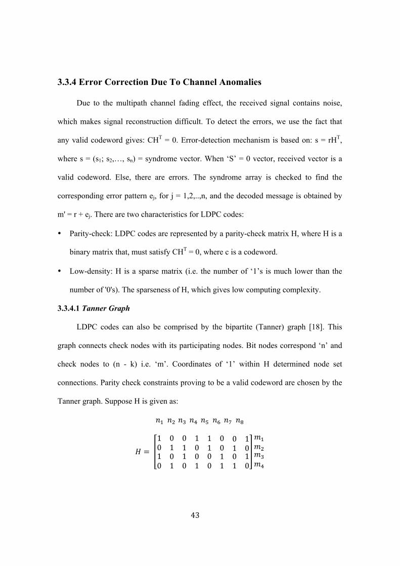
43
3.3.4 Error Correction Due To Channel Anomalies
Due to the multipath channel fading effect, the received signal contains noise,
which makes signal reconstruction difficult. To detect the errors, we use the fact that
any valid codeword gives: CHT = 0. Error-detection mechanism is based on: s = rHT,
where s = (s1; s2,…, sn) = syndrome vector. When ‘S’ = 0 vector, received vector is a
valid codeword. Else, there are errors. The syndrome array is checked to find the
corresponding error pattern ej, for j = 1,2,..,n, and the decoded message is obtained by
m' = r + ej. There are two characteristics for LDPC codes:
• Parity-check: LDPC codes are represented by a parity-check matrix H, where H is a
binary matrix that, must satisfy CHT = 0, where c is a codeword.
• Low-density: H is a sparse matrix (i.e. the number of ‘1’s is much lower than the
number of '0's). The sparseness of H, which gives low computing complexity.
3.3.4.1 Tanner Graph
LDPC codes can also be comprised by the bipartite (Tanner) graph [18]. This
graph connects check nodes with its participating nodes. Bit nodes correspond ‘n’ and
check nodes to (n - k) i.e. ‘m’. Coordinates of ‘1’ within H determined node set
connections. Parity check constraints proving to be a valid codeword are chosen by the
Tanner graph. Suppose H is given as:
𝑛! 𝑛! 𝑛! 𝑛! 𝑛! 𝑛! 𝑛! 𝑛!
𝐻 = 1 0 0 1 1 0 0 10 1 1 0 1 0 1 010
01
10
01
00
11
01
10
𝑚!𝑚!𝑚!𝑚!

44
Figure 3.5: Tanner Graph
3.3.4.2 Iterative LDPC decoding: Belief Propagation (BP) Decoding:
In LDPC Decoding, its representing bit node receives the channel value for each
bit. This value is forwarded to check nodes by bit nodes. Upon receiving the values,
parity check equations are used by checked nodes to update bit information. These
messages are sent back, having two state probabilities: 0 or 1. Check node messages
have a probability of being satisfied by parity check equations upon reception of input
messages by bit nodes. Bit nodes follow soft decision. When all the conditions are
satisfied by parity check equations using hard decision, we know that the correct
codeword is obtained [21].

45
3.4 Summary
In this section, detailed analysis of DVB-S2 system performance has been carried
out. A video is recorded and sent to TV studios for postproduction. From here, the
video is uplinked to DVB-S2 satellite after encryption. The satellite downlinks video
directly to home to the end user. The video is encoded using an LDPC encoder at
different code rates, and modulated using QPSK, 8PSK, 16APSK or 32APSK. When
the signal is transmitted through the wireless communication channel, it experiences
interference or noise due to Rician Fading Channel, Correlated Phase Noise and
AWGN. Error correction techniques are employed at reception and the signal is
regenerated by the STB to be finally viewed on television as per the Pay-TV
subscription.
46
Chapter 4
Analysis of UHD Video Broadcasting by DVB-S2
4.1 Introduction
UHD video delivery has become possible with the help of HEVC, HDMI 2.0, 6G-
SDI and more [1]. In addition, DVB-S2X has been developed especially to support
UHD video features. The trials for UHD video broadcast by DVB-S2 have also started
using UHD specific satellites [12]. Since UHD features consist of different
specifications, simulcasting of different video standards for UHD and HD will have to
be adopted. Hence, there is a need to investigate the scenario of UHD broadcasting by
DVB-S2.
4.2 Problems in DVB-S2
A DVB-S2 receiver working in Adaptive Coding and Modulation (ACM) mode,
in the future 2nd Generation of video broadcasting is required to estimate an unknown
residual gain before decoding the received signal using a LDPC code. In a mobile
communication system, the satellite link can undergo many transmission impairments
in uplink and downlink where the radio channel is usually a multipath-fading channel
causing Inter-Symbol-Interference (ISI). In addition, the received signal can be affected
by atmospheric noise and noise from the receiver [68].
In DVB-S2 systems, a time varying and correlated phase noise affects the signal.
Due to multipath fading, the Channel Impulse Response (CIR) of the signal keeps
changing continuously. Phase noise is undesirable and makes the estimation of CIR at

47
the receiver difficult. This becomes a challenge for the demodulator to acquire and
track the received signal with noise. Hence, as a result the signal is not detected and
decoded properly, leading to noise or an increase in bit errors [25].
To counterbalance this problem, a pilot-aided joint channel estimation and data
detection technique is proposed, in Section 4.4, to obtain the initial state of the channel.
Channel estimation in a coded system is important for coherent detection and
demodulation to estimate the complex impulse response of the transmitted message, so
that the original message can be regenerated from the corrupt message. This improves
the signal quality of DVB-S2 transmission and reduces the BER [69].
4.3 Importance of BER vs. SNR Calculation
Interference affects the signal quality and can result in the loss of information. In
telecommunication, interference is called noise. BER estimates the Probability of Error
(POE), which helps in predicting the signal performance in an end-to-end transmission
chain. By calculating the POE, an appropriate method is applied to improve the signal
performance at the receiver.
BER varies with SNR. In simple words, SNR is the ratio of useful data to
irrelevant data. 1:1 ratio means SNR = 0 dB i.e. Signal = Noise. This scenario is not
good and will result in high BER. SNR should be a positive figure, like 20dB, giving
low BER. Therefore, BER v/s SNR graph is plotted in a logarithmic scale, as a measure
of digital communication performance. BER cannot be reduced to zero because noise
can only be reduced to a certain level in a fixed amount of bandwidth. The information
bits contain noise. If noise is entirely removed, certain amount of information data will

48
also be lost. The acceptable BER for a video signal is 10-6 i.e. 1 bit error in 1,000,000
bits [70]. Therefore, we need to calculate at the SNR at which we will achieve this
figure, for different types of signals. In specific scenarios a lower BER value is
acceptable, depending on defined parameters.
BER vs. SNR graph simulation is important because it varies with the change in
parameters and needs to be calculated separately, to know every aspect of the signal
performance. Critical parameters have been defined to support BER vs. SNR
correlation:
4.3.1 Noise Channel
Distortion/ interference deteriorates video quality and is experienced in a wireless
communication due to:
• Rayleigh Fading (When Line of Sight is Zero, K = 0)
• Rician Fading (When Line of Sigh is not Zero, K > 0)
• Correlated Phase Noise (Which adds in the wireless communication channel)
• AWGN (gets added to the signal at the receiver)
4.3.2 MOD-COD (Modulation and Coding) scheme:
• QPSK, 8PSK, 16APSK and 32APSK
• with Code Rates of: 1/2, 3/4, 5/6, 9/10, and more
4.3.3 Type of Video
Till now there were not many types of video signals, but now we want to
determine if different video standards can result in different error rates. Parameters
given to differentiate video standards include:

49
• Resolution: (1920 x 1080), (3840 x 2160)
• Frame scan: Progressive (p) or interlaced (i)
• Frame Rate: 25, 50, 100 frames per second
• Colour profile: Rec.709 and Rec.2020
• Bit-depth: 8,10,12-bit
• Compression: MPEG-4 and HEVC
4.4 Proposed Error Reduction Method: Channel Estimation
Due to the effects of Fading, Phase Noise and AWGN, BER of the received signal
can be very high causing the Channel Impulse Response (CIR) of the signal to keep
varying; therefore, proper estimation or detection of the signal by the receiver becomes
difficult [71][72]. To help the receiver detect CIR, a method known as Channel
Estimation is used, where CIR is estimated with the help of known or pilot bits.
In this method, pilot bits are transmitted along with the information bits. These
pilot bits experience same amount of noise, as experienced by the information bits. At
the decoder, when corrupt bits are received, original channel is estimated by
characterizing known bits, which assists signal recovery. In first iteration, known bits
are used to estimate the channel.
Another iteration can be performed where the decoded bits can be treated as
‘known bits’, which will still be having some error/noise information and therefore,
noise can again be characterized and information can be used for further improving the
signal performance [72][73]. By comparing the BER achieved before and after applying

50
Channel Estimation, we can compare the BER reduction or performance gain of the
proposed method. Figure 4.1 gives a block schematic of Channel Estimation method.
Figure 4.1 Channel Estimation Block Schematic
4.5 Effect of Symbol Rate on BER
Different modulation schemes have different symbol rates. Therefore, videos are
bound to perform differently under different symbol rates, in the wireless channel.
AWGN channel passes the sum of the modulated signal and an uncorrelated
‘white’ Gaussian noise to the output. It gets added to the signal randomly, bit by bit [74].
In the analysis of the Noise (No) and bit energy (Eb) correlation,
Let No be a normally distributed random variable:
𝑁! = 𝜎!,σ = 𝑁! (4.1)
!!!!
𝑑𝐵 = !!!!
𝑑𝐵 + 10𝑙𝑜𝑔!" (𝑘) (4.2)
k = log2 M (4.3)

51
Where,
k = number of bits per symbol
M = M-ary modulation scheme
Es = Symbol energy
Eb = bit energy
For a modulated signal, therefore
𝜎 = !!!!!!
= !!!"!!!
(4.4)
For a coded signal, as the number of bits increases after coding, Energy per symbol
decreases. So we have,
Es = r * k * Eb, (4.5)
Where, r is the Euclidean distance.
𝜎 = !!!"#!!!
(4.6)
Usually, Es=1; Therefore, Noise Power:
𝜎! = !
!" !!!!
(4.7)
Where, 𝜎! = 𝜎! =!!𝜎! , Quadrature and In-phase component.

52
In a digital transmission, SNR of a signal depends on the symbol rate, not on the
bit rate. Noise effect is dependent on the bandwidth, which is influenced by the symbol
clock rate. This can be understood by equation 4.8 and 4.9, where E is the signal power
and D is period of the pulse interval.
𝑆𝑁𝑅 = !!!!= !"#$% !"#$%& !"#$%
!"#$% !"#$% (4.8)
𝑃! = !!= !
! |𝑠 𝑡 |!𝑑𝑡!! (4.9)
The signal is non-zero for ‘D’ seconds only and the mean power over an infinite
time interval is zero. As a result, the mean power during one symbol period is taken as
a measure of the signal strength. Symbol clock represents the frequency and exact
timing of the transmission of the individual symbols. At the symbol clock transitions,
the transmitted carrier is at the correct I/Q (or magnitude/phase) value to represent a
specific symbol (a specific point in the constellation). Then the values (I/Q or
magnitude/phase) of the transmitted carrier are changed to represent another symbol.
The interval between these two times is the symbol clock period, as shown in
Figure 4.2, which shows the impulse or time-domain response of a raised cosine filter.
Adjacent symbols do not interfere with each other at the symbol times because the
response equals zero at all symbol times except the center (desired) one [75][76].
Therefore, signal performance over a wireless communication channel is highly
dependent on the symbol rate or modulation scheme used, because that determines the
quality (or quantity) of information bits being transmitted/received at a time. Noise
power can be expressed in terms of the pulse interval, where
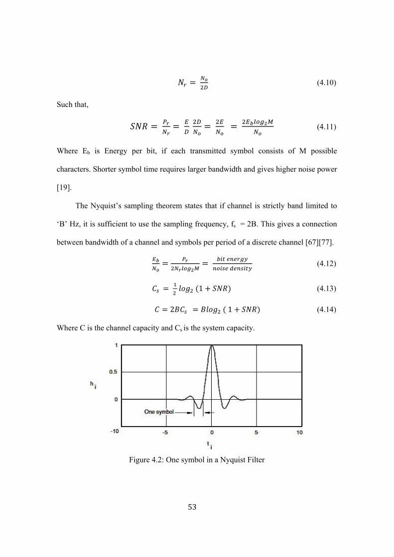
53
𝑁! = !!!!
(4.10)
Such that,
𝑆𝑁𝑅 = !!!!= !
! !!!!= !!
!! = !!!!"#!!
!! (4.11)
Where Eb is Energy per bit, if each transmitted symbol consists of M possible
characters. Shorter symbol time requires larger bandwidth and gives higher noise power
[19].
The Nyquist’s sampling theorem states that if channel is strictly band limited to
‘B’ Hz, it is sufficient to use the sampling frequency, fs = 2B. This gives a connection
between bandwidth of a channel and symbols per period of a discrete channel [67][77].
!!!!= !!
!!!!"#!!= !"# !"!#$%
!"#$% !"#$%&' (4.12)
𝐶! = !! 𝑙𝑜𝑔! (1+ 𝑆𝑁𝑅) (4.13)
𝐶 = 2𝐵𝐶! = 𝐵𝑙𝑜𝑔! ( 1+ 𝑆𝑁𝑅) (4.14)
Where C is the channel capacity and Cs is the system capacity.
Figure 4.2: One symbol in a Nyquist Filter

54
4.6 Summary
The discussion done in this chapter is aimed towards the problems related to the
UHD-DVB-S2 standard and focuses on the impact of noise on the video signal. A video
signal gets heavily distorted when passed through a radio channel of DVB-S2, where it
experiences Rician Fading and AWGN. The worst case is when a correlated phase noise
is present in the channel, which makes the CIR estimation at the receiver difficult.
There are many ways to decrease the spectral noise density. The bandwidth can be
reduced, but a minimum bandwidth has to be maintained to transmit the desired data
rate (Nyquist Criteria). The energy per bit (Eb) can be increased but interference due to
other systems can impose limitation. A lower BER can increase the Eb but capacity has
to be compromised for that.

55
Chapter 5
Proposed Video Performance Evaluation Methodology
5.1 Introduction
In this chapter a number of experiments have been proposed and carried out to test
the likelihood of system performance specifications. The standardization of DVB-S2
must take into account the varying parameters that have been used and the range of
outcomes under varying scenarios.
5.2 Future Broadcast Scenario: Multiple Video Standards
In the proposed experiments, frames from different videos are used, originally
recorded following HD and UHD standard, such as shown in Figure 5.1 and 5.2. Using
these original videos, different versions are generated having 1080p and 2160p
resolution, 25fps, 30fps and 50fps (where ever possible), and compressed using MPEG-
4 and HEVC codec. The following softwares have been used:
• Frame Rate Converter: Movavi Video Converter 4 for Mac
• HEVC Compressor: DivX Converter 10.2.1 for Mac (Compression only
available till 2160p/30fps for HEVC and 2160p/50 for MPEG-4) [78]
• Operating System: Mac OS X 10.10.3 – 64 bit and Windows 7
• BER v/s SNR graph simulated using MATLAB R2014a version for mac and
windows, limited to 8-bit (experiments done in both OS to confirm results) [79]
The reason to choose two different types of videos (one with native HD and other
with the rich colour content of UHD) is that the primary issue being investigated in this

56
thesis is the broadcast of these videos using existing resources and infrastructure, and
there are fewer chances for the same video being shot in 1080p and 2160p. It is more
likely that the existing HD 1080p content will be upscaled to a higher spatial and
temporal resolution and the new UHD 2160p content will be downscaled to a lower
resolution [80]. Therefore, the existing HD content will look less dynamic by default,
even after upscaling because its pixel density will always be lower than a video shot
using an exclusive 4K camera which enhances image sensors and other features. This is
because, Rec.2020 (for UHDTV) captures more colours as compared for Rec.709 (for
HDTV) [24][37]. Other than the two pictures shown in Figure 5.1 and 5.2, the video
also had different scenes, and by using a combination of the available colour
information in different pictures, a generalized result has been developed.
Figure 5.1: HD video frames used for experiment
Figure 5.2 UHD video frames used for experiment

57
Figure 5.3. explains the complete broadcast scenario in the presence of different
video standards coming from the source, with different TV receiver sets being used by
the consumers, taking into account the challenges faced by the DTH operator. Due to
the differences in requirements and availability per video standard, 16 versions of the
default HD and UHD video have been used, as explained in Table 5.1. A bit rate
decrease between 5% and 13% is observed, per frame (there are 25 - 50 frames per
second) when the video is compressed using an HEVC encoder as compared to MPEG-
4; while a bit rate increase from 3% to 6% per frame is observed when the frame rate is
converted from 25 to 50 fps.
Figure 5.3 Future broadcast scenario [5][81]

58
Table 5.1: Description of formation of multiple video standards
Codec Default Content
Broadcast Resolution
fps SDI TV Channel HDMI Size (MB)
1 MPEG-4 HD 1080p 25 HD HD HD 1.4a 2.75
(Default HD: 1080p/25) 2 MPEG-4 HD 1080p 50 3G HD HD+ 1.4a 2.90 (1080p/25 Upscaled to 1080p/50)
3 MPEG-4 HD 2160p 25 6G UHD HD 1.4a 8.55 (1080p/25 Upscaled to 2160p/25)
4 MPEG-4 HD 2160p 50 12G UHD HD+ 2 9.10 (1080p/25 Upscaled to 2160p/50)
5 MPEG-4 UHD 1080p 25 HD HD HD 1.4a 2.93 (2160p/25 Downscaled to 1080p/25)
6 MPEG-4 UHD 1080p 50 3G HD HD 1.4a 3.01 (2160p/25 Downscaled to 1080p/50)
7 MPEG-4 UHD 2160p 25 6G UHD UHD 1.4a 8.70 (Default UHD: 2160p/25)
8 MPEG-4 UHD 2160p 50 12G UHD UHD 2 9.10 (2160p/25 Upscaled to 2160p/50)
9 HEVC HD 1080p 25 HD HD HD 1.4a 2.40 (Default HD: 1080p/25)
10 HEVC HD 1080p 50 3G HD HD+ 1.4a 2.55 (1080p/25 Upscaled to 1080p/50)
11 HEVC HD 2160p 25 6G UHD HD 1.4a 7.55 (1080p/25 Upscaled to 2160p/25)
12 HEVC HD 2160p 30 6G UHD HD+ 1.4a 7.90 (1080p/25 UP/S 2160p/30. DivX Converter does not support 2160p/50 for HEVC at the moment) [78]
13 HEVC UHD 1080p 25 HD HD UHD 1.4a 2.73 (2160p/25 Downscaled to 1080p/25)
14 HEVC UHD 1080p 50 3G HD UHD 1.4a 2.90 (2160p/25 Downscaled to 1080p/50)
15 HEVC UHD 2160p 25 6G UHD UHD 1.4a 8.30 (Default UHD: 2160p/25)
16 HEVC UHD 2160p 30 6G UHD UHD 1.4a 8.65 2160p/25 UP/S 2160p/30. DivX Converter does not support 2160p/50 for HEVC at the moment [78]

59
5.3 Video Quality Assessment
There are many ways to do a video quality assessment. One of the most common
methods is measuring the Peak Signal to Noise Ratio (PSNR) of a video [83]. However,
since BER vs. SNR has been computed in this research work, another calculation of
PSNR is not required because it comes under the umbrella of SNR. Therefore, first,
video assessment has been done in terms of colour range because it consumes video’s
pixel depth, which contributes towards the size in Megabyte (MB) i.e. bit rate,
ultimately leading to bit error rate and wider bandwidth. Figure 5.4 to 5.7 give
histograms of video frames shown in Figure 5.1 and 5.2 respectively, varying in
parameter, simulated using MATLAB. X-axis has a range of 0 to 255, where each
decimal number represents a colour shade included in the Rec.709 standard. Y-axis is a
measure of how many times a particular colour is used in the video frame. Since
MATLAB is currently limited to reading a video of 8-bit depth, and a broadcaster’s
infrastructure is also limited to 8-bit depth, only 8-bit depth videos have been included
in this experiment.
The results show that the HD video has occupied a lower range of colours and
utilized the same colour again and again. In other words, the video frame of 1080p is
composed of limited colours, mostly green, blue, orange and its shades. The same is
observed for its upscaled version of 2160p. When it comes to UHD, the histogram has
fewer peaks across the Y-axis and is more widely spread across the X-axis. This means
that one frame of either 1080p or 2160p is composed of a wide range of colours, like,
green, purple, red, white, blue, black and more.

60
Figure 5.4: Colour range of HEVC HD 1080/25p videos
Figure 5.5: Colour range of HEVC HD 2160/25p videos
Figure 5.6: Colour range of HEVC UHD 1080/25p videos
Figure 5.7: Colour range of HEVC UHD 2160/25p videos
0
2
4
6
8
10
12
14 x 104
Colours
0 50 100 150 200 250
0
2
4
6
8
10
12
14 x 104
0 50 100 150 200 250
0
2
4
6
8
10
12
14 x 104
0 50 100 150 200 250
0
2
4
6
8
10
12
14 x 104
0 50 100 150 200 250
0
2
4
6
8
10
12
14 x 104
0 50 100 150 200 250
0
2
4
6
8
10
12
14 x 104
0 50 100 150 200 250
0
2
4
6
8
10
12
14 x 104
0 50 100 150 200 250
0
2
4
6
8
10
12
14 x 104
0 50 100 150 200 250

61
5.4 Video Performance Assessment: System Model
Once all the video samples are ready to be experimented, pixel information is
extracted from the frames in the range of 0-255. This value is converted to binary bits
and reformed into MPEG-Transport Stream (TS) in the form of Base Band Frame or
BBFRAME as a part of stream adaptation by DVB-S2 to enter through the BCH
Encoder [82], as shown in Figure 5.8.
Figure 5.8: MPEG-TS BBFRAME [82]
The length of KBCH or BBFRAME or the input to the BCH encoder varies with the
code rate as given in Table 5.2 for 3/4, 5/6 and 9/10 code rates.
Table 5.2: Coding Parameters for FEC Block size = 64,800 [25]
LDPC Code BHC Uncoded
Block (KBCH) BCH Coded block (NBCH)
LDPC Coded Block (NLDPC)
3/4 48,408 48,600 64,800 5/6 53,840 54,000 64,800 9/10 58,192 58,320 64,800

62
A BBFRAME or Base Band Frame or KBCH is composed of the following:
• BBHEADER consists of 80 bits
• Data generator = 188 bytes x 8 bits = 1504 bits
• DATA FIELD represents the number of MPEG packets that can be fitted in one
BBFRAME and is given by = !!"# !!"!"#$
• ZERO PADDING = KBCH – [(Number of packets * 1504 ) + 80]
Performance evaluation is done using MATLAB for DVB-S2, using QPSK,
8PSK, 16APSK and 32APSK modulation scheme, with a code rate of 3/4, 5/6 and 9/10.
FEC block size = 64800, using BCH + LDPC encoder and a soft-decision decoder, in
the presence of AWGN, Rician Fading Channel and a Correlated Phase Noise. For this
simulation, the fading factor is generated randomly and multiplied by every incoming
frame but is constant over one entire frame. Next, the faded codeword is affected by a
time varying and correlated phase noise. This phase noise is deterministic for better
channel estimation simulation results. At the receiver, AWGN is added to the message
and it affects the signal bit by bit. We generate noise randomly and add it to every bit in
the message independently [83]. Channel estimation is performed on the received bits
with the help of known pilot bits. Therefore, the estimated Channel Impulse Response
(CIR) of the varying signal is computed as the mean of all the pilot bits. After this, pilot
bits are removed from the received signal. The computed CIR is fed to the equalizer in
which the estimated channel value equalizes (divides) every bit of the received message
and compensates for noise. The equalizer output is demodulated which gives the Log
Likelihood Ratio (LLR) values. These LLRs are decoded and the message is recovered
63
but there are still errors in it. The number of error bits with increasing signal to noise
ratio is plotted. BER varies with SNR; thus, BER v/s SNR graph is plotted in
logarithmic scale, as a measure of digital communication performance. The acceptable
BER for a video signal is 10-6 i.e. 1 bit error in 1,000,000 bits for a video [71].
Therefore, we need to calculate the SNR at which we will achieve this value for
different signals. Let us assume transmission of LDPC encoded and complex
modulated symbols over a Rician Fading Channel and AWGN channel affected by
phase noise:
Coded and Modulated message: C = [ c1, c2, ...., ck ];
Pilot bits: P = [ P1, P2, ...., Pk ]
Transmitted message: M = [P C] (5.1)
‘M’ is passed through the Rician channel ‘h’ where correlated phase noise ‘e jΦk’ is
added to it, and given by = M * e jΦk (5.2)
Channel: h = [ h1, h2, ...., hk ] = h [M * e jΦk] (5.3)
Channel phases: q = [ q0, q1, ...., qk-1 ] = h [M * e jΦk]e jq (5.4)
Phase noise according to Wiener random walk model described by:
qK = qK-1 + ΛK (5.5)
Where: Λk: white real Gaussian process: Λk ~ N(0, σΛ)
Finally, AWGN ‘n’ is added at the receiver:
Noise: n = [ n1, n2, ...., nk ]

64
The received message is:
Y = RM (t) = h [M * e jΦk]e jq + ΛK (5.6)
Using equation (5.1) in (5.6),
Y = RM (t + 1) = h [PC * e jΦk]e jq + ΛK
= h [PC * e j (Φk + q) ] + ΛK (5.7)
Channel estimation can be done by:
CIR = average (Y1-P / P) (5.8)
Equalizer: E = Y (P-1)-k / CIR (5.9)
Channel estimation and decoding techniques are implemented to compute the CIR
of the signal at the receiver. Channel Estimation helps in reducing the BER to 10-6, for
Rician factor ‘K=5’ but not for ‘K=0’. This is because as ‘K’ increases, the ratio of the
power received via the LOS path to the power contribution of the non-LOS paths,
increases. If ‘K’ is high, the Pr (Received power) or Es (Energy per symbol) or Eb
(Energy per bit) is high. This gives a higher SNR, which ultimately decreases the BER
as per Equation 5.5, where ‘B’ is the total bandwidth and ‘Ts’ symbol time and ‘Tb’ is
bit time. BER decreases because as Es increases, the distance between adjacent symbol
increases and correlation decreases. This bootstraps the decoder in signal recovery.
𝑆𝑁𝑅 = !!!!!
= !!!!!"!
= !!!!!"!
(5.10)

65
5.5 Experiment 1: In the presence of AWGN only
In Experiment 1, performances of two videos have been analyzed in the presence
of AWGN. Videos used: HEVC HD 1080p/25 and HEVC UHD 2160p/25.
5.5.1 Result Summary - 1
As SNR increases, BER decreases because when signal power is more than the
noise power, signal detection and decoding is improved, resulting in a lower BER.
There is a significant increase in the BER rate of UHD as compared to HD, for QPSK
and 8PSK, as compared to 16APSK and 32APSK. UHD video (HEVC UHD 2160/25p)
has a higher BER than HD. This can be seen from Figure 5.12 at SNR = 9.36 dB, BER
for HD is in the vicinity of 10-5, while BER for UHD is in the vicinity of 10-4, which is
a large difference and can result in an increase of the overall cost of transmission power
to achieve the desired BER [84]. Complete results of this experiment are given from
Figure 5.9 to 5.20.
The maximum increase in BER for UHD, as compared to HD, is seen for code
rate = 5/6. Code rate 3/4 also shows an increase in BER, but less than 5/6. While code
rate 9/10 rate shows the lowest error rate difference.
" Result: UHD has a higher BER than HD in QPSK and 8PSK
" More analysis is done for 8PSK-5/6, with respect to HFR, in Experiment 2
" Cost implications are discussed in Section 6.7

66
Figure 5.9: BER vs. SNR of UHD and
HD for QPSK-3/4, with AWGN Figure 5.10: BER vs. SNR of UHD and
HD for 8PSK-3/4, with AWGN
Figure 5.11: BER vs. SNR of UHD and
HD for QPSK-5/6, with AWGN Figure 5.12: BER vs. SNR of UHD and
HD for 8PSK-5/6, with AWGN
Figure 5.13: BER vs. SNR of UHD and
HD for QPSK-9/10, with AWGN Figure 5.14: BER vs. SNR of UHD and
HD for 8PSK-9/10, with AWGN
3.84 3.86 3.88 3.9 3.92 3.94 3.96 3.98 410−6
10−5
10−4
10−3
10−2
10−1
100
SNR (in dB)
BE
R
QPSK 3/4, AWGN
HEVC HD 1080/25pHEVC UHD 2160/25p
7.81 7.82 7.83 7.84 7.85 7.86 7.87 7.88 7.89 7.9 7.9110−6
10−5
10−4
10−3
10−2
10−1
100
8PSK 3/4, AWGN
SNR (in dB)
BE
R
HEVC HD 1080/25pHEVC UHD 2160/25p
5.08 5.09 5.1 5.11 5.12 5.13 5.14 5.15 5.1610−6
10−5
10−4
10−3
10−2
10−1
100
QPSK 5/6, AWGN
SNR (in dB)
BE
R
HEVC HD 1080/25pHEVC UHD 2160/25p
9.26 9.28 9.3 9.32 9.34 9.36 9.3810−6
10−5
10−4
10−3
10−2
10−1
100
8PSK 5/6, AWGN
SNR (in dB)
BE
R
HEVC HD 1080/25pHEVC UHD 2160/25p
6.32 6.33 6.34 6.35 6.36 6.37 6.38 6.39 6.410−6
10−5
10−4
10−3
10−2
10−1
100
QPSK 9/10, AWGN
SNR (in dB)
BE
R
HEVC HD 1080/25pHEVC UHD 2160/25p
10.86 10.87 10.88 10.89 10.9 10.91 10.92 10.93 10.9410−6
10−5
10−4
10−3
10−2
10−1
100
8PSK 9/10, AWGN
SNR (in dB)
BE
R
HEVC HD 1080/25pHEVC UHD 2160/25p
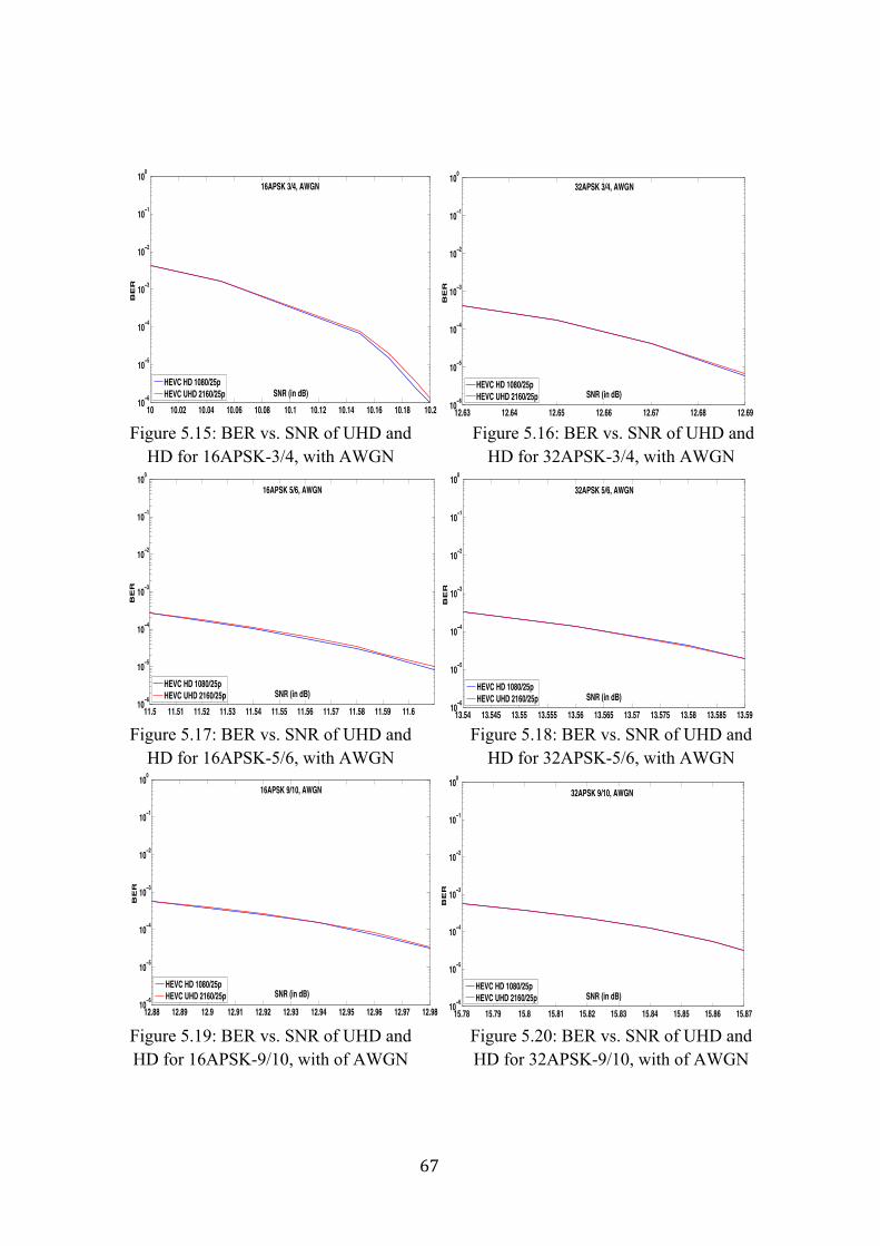
67
Figure 5.15: BER vs. SNR of UHD and
HD for 16APSK-3/4, with AWGN Figure 5.16: BER vs. SNR of UHD and
HD for 32APSK-3/4, with AWGN
Figure 5.17: BER vs. SNR of UHD and
HD for 16APSK-5/6, with AWGN Figure 5.18: BER vs. SNR of UHD and
HD for 32APSK-5/6, with AWGN
Figure 5.19: BER vs. SNR of UHD and HD for 16APSK-9/10, with of AWGN
Figure 5.20: BER vs. SNR of UHD and HD for 32APSK-9/10, with of AWGN
10 10.02 10.04 10.06 10.08 10.1 10.12 10.14 10.16 10.18 10.210−6
10−5
10−4
10−3
10−2
10−1
100
16APSK 3/4, AWGN
SNR (in dB)
BE
R
HEVC HD 1080/25pHEVC UHD 2160/25p
12.63 12.64 12.65 12.66 12.67 12.68 12.6910−6
10−5
10−4
10−3
10−2
10−1
100
32APSK 3/4, AWGN
SNR (in dB)
BE
R
HEVC HD 1080/25pHEVC UHD 2160/25p
11.5 11.51 11.52 11.53 11.54 11.55 11.56 11.57 11.58 11.59 11.610−6
10−5
10−4
10−3
10−2
10−1
100
16APSK 5/6, AWGN
SNR (in dB)
BE
R
HEVC HD 1080/25pHEVC UHD 2160/25p
13.54 13.545 13.55 13.555 13.56 13.565 13.57 13.575 13.58 13.585 13.5910−6
10−5
10−4
10−3
10−2
10−1
100
32APSK 5/6, AWGN
SNR (in dB)
BE
R
HEVC HD 1080/25pHEVC UHD 2160/25p
12.88 12.89 12.9 12.91 12.92 12.93 12.94 12.95 12.96 12.97 12.9810−6
10−5
10−4
10−3
10−2
10−1
100
16APSK 9/10, AWGN
SNR (in dB)
BE
R
HEVC HD 1080/25pHEVC UHD 2160/25p
15.78 15.79 15.8 15.81 15.82 15.83 15.84 15.85 15.86 15.8710−6
10−5
10−4
10−3
10−2
10−1
100
32APSK 9/10, AWGN
SNR (in dB)
BE
R
HEVC HD 1080/25pHEVC UHD 2160/25p

68
5.6 Experiment 2: High Frame Rate Videos
In Experiment 1, QPSK and 8PSK show increased BER when a UHD video is
broadcasted, as compared to HD, in the presence of AWGN only. In Experiment 2, 16
different types of videos are transmitted through an 8PSK modulator, using code rate
5/6, in the presence of AWGN. These different videos comprise of HD and UHD video
content, both having (1920x1080) and (3840x2160) resolution; 25 and 50 frames per
second in progressive mode; using MEPG-4 and HEVC compression method as given
in Table 5.1 in section 5.2.
5.6.1 Result Summary - 1
The most important finding of this experiment is that the BER of videos having
50fps (or 30fps) is lower than 25fps. This is because as the frame rate increases, even
though the number of frames increases, marking an increase in the total video size, but
due to compression, the amount of data that every frame carries decreases [85]. In a
compressed video, every frame only carries the difference between the current and
reference frame. Therefore, as a result of compression, the bits per frame decreases as
the number of frames increases. This makes the data less susceptible to noise and
bootstraps the signal recovery at the receiver. This can be understood from Figure 5.21.
Hence, the signal performance of a video with more frames is better than the same
video having fewer frames with a lot of data per frame [86]. The results are the same
for HEVC and MPEG-4 video compression as shown in Figure 5.22.
" Result: BER decreases as frame rate increases

69
Figure 5.21: Understanding frame rate: For videos (motion based), as frame rate
increases, bit rate decreases [85]
5.6.2 Result Summary - 2
UHD 2160p/25 video has the highest BER followed by UHD 2160p/30 (due to
the reason stated in the previous section), because it has the highest bit rate of all the
videos. The second highest is UHD 1080p/25 (and 1080p/50), which is the downscaled
version of 2160p/25. The second lowest is HD 2160p/25 (and HD 2160p/30), which is
the upscaled version of HD 1080p/25 and the video with the lowest BER is HD
1080p/25 (and HD 1080p/50).
Interestingly, it is observed that even though UHD/2160p has been converted to
UHD/1080p resolution, still its BER is higher than the HD/1080p video and this is due
to the difference in the colour pixel density or the amount of information they carry.
Therefore, if a broadcaster assumes that the signal performance or BER of a
downscaled UHD video will be similar to the HD video, might be wrong.
" Result: UHD downscaled video BER is higher than HD upscaled video
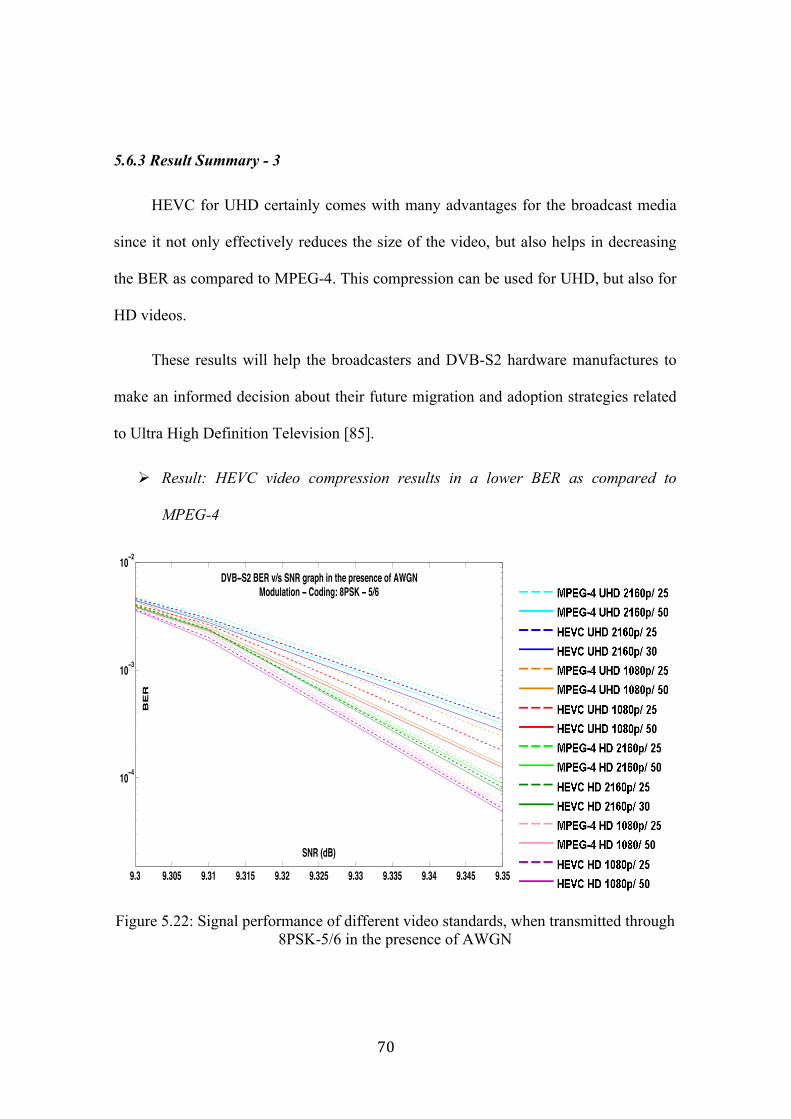
70
5.6.3 Result Summary - 3
HEVC for UHD certainly comes with many advantages for the broadcast media
since it not only effectively reduces the size of the video, but also helps in decreasing
the BER as compared to MPEG-4. This compression can be used for UHD, but also for
HD videos.
These results will help the broadcasters and DVB-S2 hardware manufactures to
make an informed decision about their future migration and adoption strategies related
to Ultra High Definition Television [85].
" Result: HEVC video compression results in a lower BER as compared to
MPEG-4
Figure 5.22: Signal performance of different video standards, when transmitted through 8PSK-5/6 in the presence of AWGN
9.3 9.305 9.31 9.315 9.32 9.325 9.33 9.335 9.34 9.345 9.35
10−4
10−3
10−2
DVB−S2 BER v/s SNR graph in the presence of AWGNModulation − Coding: 8PSK − 5/6
SNR (dB)
BE
R

71
5.7 Experiment 3: Rician Fading & Channel Estimation
In Experiment three, UHD and HD video signals are transmitted through the
wireless communication channel in the presence of Rician Fading Channel, Correlated
Phase Noise and AWGN. There are two types of Noise Channel: for K = 0 i.e. Rayleigh
Fading and for K = 5 i.e. Rician Fading. The results for these two channels are shown
separately for each MOD-COD scheme. This experiment is performed with and without
using channel estimation.
Results show that the required SNR to achieve the desired BER is higher for a
Rician Fading channel, as compared to AWGN. BER of UHD is higher than HD for
QPSK and 16APSK only, for 3/4 and 5/6 code rate, instead of QPSK and 8PSK as in
the case of AWGN only [87][88].
Figure 5.23 shows the constellation diagrams for Rician Channel, K=5 at
SNR=20dB for QPSK, 8PSK, 16APSK and 32APSK. The correlation is lower as
compared to what it is for K=0 at SNR=-10dB. When the correlation is high, there is
more degradation due to noise and a higher SNR is required to regenerate the signal.
The constellations of 8PSK and 32APSK are close to each other and the correlation is
high, as compared to QPSK and 16APSK. This is the reason that QPSK and 16APSK
are able to detect the difference between UHD and HD video pixel density. Higher
correlation results in a higher BER, therefore, the BER vs. SNR graphs (5.24-5.35)
depict exactly what a signal goes through under noise.

72
Figure 5.23: Constellation diagrams of different modulation schemes with noise, at SNR=20dB for Rician Fading Channel (K=5)
−1 −0.5 0 0.5 1−1
−0.8
−0.6
−0.4
−0.2
0
0.2
0.4
0.6
0.8
1QPSK − Rician Fading
−1 −0.5 0 0.5 1−1
−0.8
−0.6
−0.4
−0.2
0
0.2
0.4
0.6
0.8
1QPSK − Rician + Phase Noise
−15 −10 −5 0 5 10 15
−15
−10
−5
0
5
10
15
QPSK − Rician + Phase + AWGN
−1 −0.5 0 0.5 1−1
−0.8
−0.6
−0.4
−0.2
0
0.2
0.4
0.6
0.8
18PSK − Rician
−1 −0.5 0 0.5 1−1
−0.8
−0.6
−0.4
−0.2
0
0.2
0.4
0.6
0.8
1 8PSK − Rician + Phase
−15 −10 −5 0 5 10 15
−15
−10
−5
0
5
10
15
8PSK − Rician + Phase + AWGN
−1 −0.5 0 0.5 1−1
−0.8
−0.6
−0.4
−0.2
0
0.2
0.4
0.6
0.8
116APSK − Rician
−1 −0.5 0 0.5 1−1
−0.8
−0.6
−0.4
−0.2
0
0.2
0.4
0.6
0.8
132APSK − Rician + Phase
−15 −10 −5 0 5 10 15
−15
−10
−5
0
5
10
15
16APSK − Rician + Phase + AWGN
−1 −0.5 0 0.5 1−1
−0.8
−0.6
−0.4
−0.2
0
0.2
0.4
0.6
0.8
132APSK − Rician
−1 −0.5 0 0.5 1−1
−0.8
−0.6
−0.4
−0.2
0
0.2
0.4
0.6
0.8
132APSK − Rician + Phase
−15 −10 −5 0 5 10 15
−15
−10
−5
0
5
10
15
32APSK − Rician + Phase + AWGN

73
(a) (b)
Figure 5.24: BER vs. SNR for QPSK-3/4 (a) Rayleigh Fading (b) Rician Fading
(a) (b)
Figure 5.25: BER vs. SNR for QPSK-5/4 (a) Rayleigh Fading (b) Rician Fading
(a) (b)
Figure 5.26: BER vs. SNR for QPSK-9/10 (a) Rayleigh Fading (b) Rician Fading
−10 −5 0 5 10 15 2010−6
10−5
10−4
10−3
10−2
10−1
100
SNR (dB)
BE
R
QPSK 3/4, AWGN + Rayleigh Fading (K=0) + Phase Noise
HD Video, Without Channel EstimationUHD Video, Without Channel EstimationHD Video, With Channel EstimationUHD Video, With Channel Estimation
−10 −5 0 5 10 15 2010−6
10−5
10−4
10−3
10−2
10−1
100QPSK 3/4, AWGN + Rician Fading Channel (K=5) + Phase Noise
SNR (in dB)
BE
R
HD video, Without Channel EstimationUHD video, Without Channel EstimationHD video, With Channel EstimationUHD video, With Channel Estimation
−10 −5 0 5 10 15 2010−6
10−5
10−4
10−3
10−2
10−1
100 QPSK 5/6, AWGN + Rayleigh Fading (K=0) + Phase Noise
SNR (dB)
BE
R
HD Video, Without Channel EstimationUHD Video, Without Channel EstimationHD Video, With Channel EstimationUHD Video, With Channel Estimation
−10 −5 0 5 10 15 2010−6
10−5
10−4
10−3
10−2
10−1
100 QPSK 5/6, AWGN + Rician Fading Channel (K=5) + Phase Noise
SNR (in dB)
BE
R
HD video, Without Channel EstimationUHD video, Without Channel EstimationHD video, With Channel EstimationUHD video, With Channel Estimation
−10 −5 0 5 10 15 2010−6
10−5
10−4
10−3
10−2
10−1
100 QPSK 9/10, AWGN + Rayleigh Fading (K=0) + Phase Noise
SNR (dB)
BE
R
HD Video, Without Channel EstimationUHD Video, Without Channel EstimationHD Video, With Channel EstimationUHD Video, With Channel Estimation
−10 −5 0 5 10 15 2010−6
10−5
10−4
10−3
10−2
10−1
100 QPSK 9/10, AWGN + Rician Fading Channel (K=5) + Phase Noise
SNR (in dB)
BE
R
HD video, Without Channel EstimationUHD video, Without Channel EstimationHD video, With Channel EstimationUHD video, With Channel Estimation

74
(a) (b)
Figure 5.27: BER vs. SNR for 8PSK-3/4 (a) Rayleigh Fading (b) Rician Fading
(a) (b)
Figure 5.28: BER vs. SNR for 8PSK-5/6 (a) Rayleigh Fading (b) Rician Fading
(a) (b)
Figure 5.29: BER vs. SNR for 8PSK-9/10 (a) Rayleigh Fading (b) Rician Fading
−10 −5 0 5 10 15 2010−6
10−5
10−4
10−3
10−2
10−1
100 8PSK 3/4, AWGN + Rayleigh Fading (K=0) + Phase Noise
SNR (dB)
BE
R
HD Video, Without Channel EstimationUHD Video, Without Channel EstimationHD Video, With Channel EstimationUHD Video, With Channel Estimation
−10 −5 0 5 10 15 2010−6
10−5
10−4
10−3
10−2
10−1
100 8PSK 3/4, AWGN + Rician Fading Channel (K=5) + Phase Noise
SNR (in dB)
BE
R
HD video, Without Channel EstimationUHD video, Without Channel EstimationHD video, With Channel EstimationUHD video, With Channel Estimation
−10 −5 0 5 10 15 2010−6
10−5
10−4
10−3
10−2
10−1
100 8PSK 5/6, AWGN + Rayleigh Fading (K=0) + Phase Noise
SNR (dB)
BE
R
HD Video, Without Channel EstimationUHD Video, Without Channel EstimationHD Video, With Channel EstimationUHD Video, With Channel Estimation
−10 −5 0 5 10 15 2010−6
10−5
10−4
10−3
10−2
10−1
100 8PSK 5/6, AWGN + Rician Fading Channel (K=5) + Phase Noise
SNR (in dB)
BE
R
HD video, Without Channel EstimationUHD video, Without Channel EstimationHD video, With Channel EstimationUHD video, With Channel Estimation
−10 −5 0 5 10 15 2010−6
10−5
10−4
10−3
10−2
10−1
100 8PSK 9/10, AWGN + Rayleigh Fading (K=0) + Phase Noise
SNR (dB)
BE
R
HD Video, Without Channel EstimationUHD Video, Without Channel EstimationHD Video, With Channel EstimationUHD Video, With Channel Estimation
−10 −5 0 5 10 15 2010−6
10−5
10−4
10−3
10−2
10−1
100 8PSK 9/10, AWGN + Rician Fading Channel (K=5) + Phase Noise
SNR (in dB)
BE
R
HD video, Without Channel EstimationUHD video, Without Channel EstimationHD video, With Channel EstimationUHD video, With Channel Estimation

75
(a) (b)
Figure 5.30: BER vs. SNR for 16APSK-3/4 (a) Rayleigh Fading (b) Rician Fading
(a) (b)
Figure 5.31: BER vs. SNR for 16APSK-5/6 (a) Rayleigh Fading (b) Rician Fading
(a) (b)
Figure 5.32: BER vs. SNR for 16APSK-9/10 (a) Rayleigh Fading (b) Rician Fading
−10 −5 0 5 10 15 2010−6
10−5
10−4
10−3
10−2
10−1
10016APSK 3/4, AWGN + Rayleigh Fading (K=0) + Phase Noise
SNR (dB)
BE
R
HD Video, Without Channel EstimationUHD Video, Without Channel EstimationHD Video, With Channel EstimationUHD Video, With Channel Estimation
−10 −5 0 5 10 15 2010−6
10−5
10−4
10−3
10−2
10−1
10016APSK 3/4, AWGN + Rician Fading Channel (K=5) + Phase Noise
SNR (dB)
BE
R
HD video, Without Channel EstimationUHD video, Without Channel EstimationHD video, With Channel EstimationUHD video, With Channel Estimation
−10 −5 0 5 10 15 2010−6
10−5
10−4
10−3
10−2
10−1
100 16APSK 5/6, AWGN + Rayleigh Fading (K=0) + Phase Noise
SNR (dB)
BE
R
HD Without, Without Channel EstimationUHD Without, Without Channel EstimationHD With, With Channel EstimationUHD With, With Channel Estimation
−10 −5 0 5 10 15 2010−6
10−5
10−4
10−3
10−2
10−1
10016APSK 5/6, AWGN + Rician Fading Channel (K=5) + Phase Noise
SNR (dB)
BE
R
HD video, Without Channel EstimationUHD video, Without Channel EstimationHD video, With Channel EstimationUHD video, With Channel Estimation
−10 −5 0 5 10 15 2010−6
10−5
10−4
10−3
10−2
10−1
100 16APSK 9/10, AWGN + Rayleigh Fading (K=0) + Phase Noise
SNR (dB)
BE
R
HD Video, Without Channel EstimationUHD Video, Without Channel EstimationHD Video, With Channel EstimationUHD Video, With Channel Estimation
−10 −5 0 5 10 15 2010−6
10−5
10−4
10−3
10−2
10−1
100 16APSK 9/10, AWGN + Rician Fading Channel (K=5) + Phase Noise
SNR (in dB)
BE
R
HD video, Without Channel EstimationUHD video, Without Channel EstimationHD video, With Channel EstimationUHD video, With Channel Estimation

76
(a) (b)
Figure 5.33: BER vs. SNR for 32APSK-3/4 (a) Rayleigh Fading (b) Rician Fading
(a) (b)
Figure 5.34: BER vs. SNR for 32APSK-5/6 (a) Rayleigh Fading (b) Rician Fading
(a) (b)
Figure 5.35: BER vs. SNR for 32APSK-9/10 (a) Rayleigh Fading (b) Rician Fading
−10 −5 0 5 10 15 2010−6
10−5
10−4
10−3
10−2
10−1
100 32APSK 3/4, AWGN + Rayleigh Fading (K=0) + Phase Noise
SNR (dB)
BE
R
HD Video, Without Channel EstimationUHD Video, Without Channel EstimationHD Video, With Channel EstimationUHD Video, With Channel Estimation
−10 −5 0 5 10 15 2010−6
10−5
10−4
10−3
10−2
10−1
100 32APSK 3/4, AWGN + Rician Fading Channel (K=5) + Phase Noise
SNR (in dB)
BE
R
HD video, Without Channel EstimationUHD video, Without Channel EstimationHD video, With Channel EstimationUHD video, With Channel Estimation
−10 −5 0 5 10 15 2010−6
10−5
10−4
10−3
10−2
10−1
100 32APSK 5/6, AWGN + Rayleigh Fading (K=0) + Phase Noise
SNR (dB)
BE
R
HD Video, Without Channel EstimationUHD Video, Without Channel EstimationHD Video, With Channel EstimationUHD Video, With Channel Estimation
−10 −5 0 5 10 15 2010−6
10−5
10−4
10−3
10−2
10−1
100 32APSK 5/6, AWGN + Rician Fading Channel (K=5) + Phase Noise
SNR (in dB)
BE
R
HD video, Without Channel EstimationUHD video, Without Channel EstimationHD video, With Channel EstimationUHD video, With Channel Estimation
−10 −5 0 5 10 15 2010−6
10−5
10−4
10−3
10−2
10−1
100 32APSK 9/10, AWGN + Rayleigh Fading (K=0) + Phase Noise
SNR (dB)
BE
R
HD Video, Without Channel EstimationUHD Video, Without Channel EstimationHD Video, With Channel EstimationUHD Video, With Channel Estimation
−10 −5 0 5 10 15 2010−6
10−5
10−4
10−3
10−2
10−1
100 32APSK 9/10, AWGN + Rician Fading Channel (K=5) + Phase Noise
SNR (in dB)
BE
R
HD video, Without Channel EstimationUHD video, Without Channel EstimationHD video, With Channel EstimationUHD video, With Channel Estimation
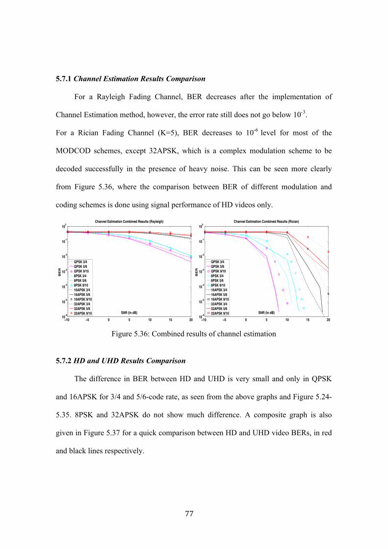
77
5.7.1 Channel Estimation Results Comparison
For a Rayleigh Fading Channel, BER decreases after the implementation of
Channel Estimation method, however, the error rate still does not go below 10-3.
For a Rician Fading Channel (K=5), BER decreases to 10-6 level for most of the
MODCOD schemes, except 32APSK, which is a complex modulation scheme to be
decoded successfully in the presence of heavy noise. This can be seen more clearly
from Figure 5.36, where the comparison between BER of different modulation and
coding schemes is done using signal performance of HD videos only.
Figure 5.36: Combined results of channel estimation
5.7.2 HD and UHD Results Comparison
The difference in BER between HD and UHD is very small and only in QPSK
and 16APSK for 3/4 and 5/6-code rate, as seen from the above graphs and Figure 5.24-
5.35. 8PSK and 32APSK do not show much difference. A composite graph is also
given in Figure 5.37 for a quick comparison between HD and UHD video BERs, in red
and black lines respectively.
−10 −5 0 5 10 15 2010−6
10−5
10−4
10−3
10−2
10−1
100Channel Estimation Combined Results (Rayleigh)
SNR (in dB)
BE
R
QPSK 3/4QPSK 5/6QPSK 9/108PSK 3/48PSK 5/68PSK 9/1016APSK 3/416APSK 5/616APSK 9/1032APSK 3/432APSK 5/632APSK 9/10
−10 −5 0 5 10 15 2010−6
10−5
10−4
10−3
10−2
10−1
100Channel Estimation Combined Results (Rician)
SNR (in dB)
BE
R
QPSK 3/4QPSK 5/6QPSK 9/108PSK 3/48PSK 5/68PSK 9/1016APSK 3/416APSK 5/616APSK 9/1032APSK 3/432APSK 5/632APSK 9/10

78
A small increase in BER for QPSK and 16APSK can change the required SNR or
the transmission power to achieve a certain BER, resulting in an overall increase in the
transmission cost of a UHD video in the future, as discussed in Section 6.7.
Figure 5.37: Channel Estimation results: UHD (black) vs. HD (red)
5.7.3 Effect of code rate
When BER vs. SNR graph for a particular modulation scheme and different code
rates is plotted, for HD after using Channel estimation, it is observed that as the code
rate increases, the required SNR to achieve a particular BER also increases. This is
because, as the code rate increase, system complexity also increases and a higher signal
power is required to detect and decode the signal at the receiver, as seen in the plots in
Figure 5.38.
−10 −5 0 5 10 15 2010−6
10−5
10−4
10−3
10−2
10−1
100 Channel Estimation Combined Results (Rician)−UHD
SNR (in dB)
BER
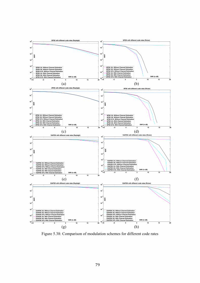
79
(a) (b)
(c) (d)
(e) (f)
(g) (h)
Figure 5.38: Comparison of modulation schemes for different code rates
−10 −5 0 5 10 15 2010−6
10−5
10−4
10−3
10−2
10−1
100
SNR (in dB)
BE
R
QPSK with different code rates (Rayleigh)
QPSK 3/4, Without Channel EstimationQPSK 5/6, Without Channel EstimationQPSK 9/10, Without Channel EstimationQPSK 3/4, With Channel EstimationQPSK 5/6, With Channel EstimationQPSK 9/10, With Channel Estimation
−10 −5 0 5 10 15 2010−6
10−5
10−4
10−3
10−2
10−1
100
SNR (in dB)
BER
QPSK with different code rates (Rician)
QPSK 3/4, Without Channel EstimationQPSK 5/6, Without Channel EstimationQPSK 9/10, Without Channel EstimationQPSK 3/4, With Channel EstimationQPSK 5/6, With Channel EstimationQPSK 9/10, With Channel Estimation
−10 −5 0 5 10 15 2010−6
10−5
10−4
10−3
10−2
10−1
100 8PSK with different code rates (Rayleigh)
SNR (in dB)
BE
R
8PSK 3/4, Without Channel Estimation8PSK 5/6, Without Channel Estimation8PSK 9/10, Without Channel Estimation8PSK 3/4, With Channel Estimation8PSK 5/6, With Channel Estimation8PSK 9/10, With Channel Estimation
−10 −5 0 5 10 15 2010−6
10−5
10−4
10−3
10−2
10−1
100
SNR (in dB)
BER
8PSK with different code rates (Rician)
8PSK 3/4, Without Channel Estimation8PSK 5/6, Without Channel Estimation8PSK 9/10, Without Channel Estimation8PSK 3/4, With Channel Estimation8PSK 5/6, With Channel Estimation8PSK 9/10, With Channel Estimation
−10 −5 0 5 10 15 2010−6
10−5
10−4
10−3
10−2
10−1
100
SNR (in dB)
BE
R
16APSK with different code rates (Rayleigh)
16APSK 3/4, Without Channel Estimation16APSK 5/6, Without Channel Estimation16APSK 9/10, Without Channel Estimation16APSK 3/4, With Channel Estimation16APSK 5/6, With Channel Estimation16APSK 9/10, With Channel Estimation −10 −5 0 5 10 15 2010−6
10−5
10−4
10−3
10−2
10−1
10016APSK with different code rates (Rician)
SNR (in dB)
BER
16APSK 3/4, Without Channel Estimation16APSK 5/6, Without Channel Estimation16APSK 9/10, Without Channel Estimation16APSK 3/4, With Channel Estimation16APSK 5/6, With Channel Estimation16APSK 9/10, With Channel Estimation
−10 −5 0 5 10 15 2010−6
10−5
10−4
10−3
10−2
10−1
100
SNR (in dB)
BE
R
32APSK with different code rates (Rayleigh)
32APSK 3/4, Without Channel Estimation32APSK 5/6, Without Channel Estimation32APSK 9/10, Without Channel Estimation32APSK 3/4, With Channel Estimation32APSK 5/6, With Channel Estimation32APSK 9/10, With Channel Estimation
−10 −5 0 5 10 15 2010−6
10−5
10−4
10−3
10−2
10−1
100
SNR (in dB)
BER
32APSK with different code rates (Rician)
32APSK 3/4, Without Channel Estimation32APSK 5/6, Without Channel Estimation32APSK 9/10, Without Channel Estimation32APSK 3/4, With Channel Estimation32APSK 5/6, With Channel Estimation32APSK 9/10, With Channel Estimation
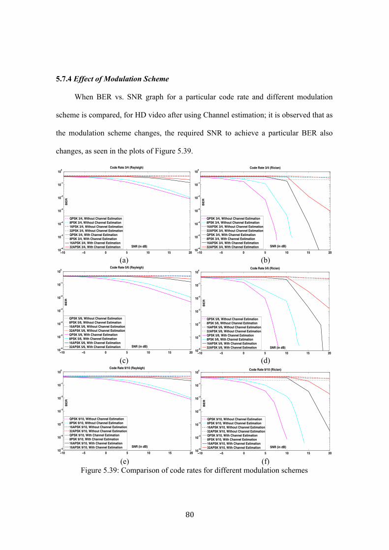
80
5.7.4 Effect of Modulation Scheme
When BER vs. SNR graph for a particular code rate and different modulation
scheme is compared, for HD video after using Channel estimation; it is observed that as
the modulation scheme changes, the required SNR to achieve a particular BER also
changes, as seen in the plots of Figure 5.39.
(a) (b)
(c) (d)
(e) (f)
Figure 5.39: Comparison of code rates for different modulation schemes
−10 −5 0 5 10 15 2010−6
10−5
10−4
10−3
10−2
10−1
100
SNR (in dB)
BE
R
Code Rate 3/4 (Rayleigh)
QPSK 3/4, Without Channel Estimation8PSK 3/4, Without Channel Estimation16PSK 3/4, Without Channel Estimation32PSK 3/4, Without Channel EstimationQPSK 3/4, With Channel Estimation8PSK 3/4, With Channel Estimation16APSK 3/4, With Channel Estimation32APSK 3/4, With Channel Estimation
−10 −5 0 5 10 15 2010−6
10−5
10−4
10−3
10−2
10−1
100Code Rate 3/4 (Rician)
SNR (in dB)
BE
R
QPSK 3/4, Without Channel Estimation8PSK 3/4, Without Channel Estimation16APSK 3/4, Without Channel Estimation32APSK 3/4, Without Channel EstimationQPSK 3/4, With Channel Estimation8PSK 3/4, With Channel Estimation16APSK 3/4, With Channel Estimation32APSK 3/4, With Channel Estimation
−10 −5 0 5 10 15 2010−6
10−5
10−4
10−3
10−2
10−1
100
SNR (in dB)
BE
R
Code Rate 5/6 (Rayleigh)
QPSK 5/6, Without Channel Estimation8PSK 5/6, Without Channel Estimation16APSK 5/6, Without Channel Estimation32APSK 5/6, Without Channel EstimationQPSK 5/6, With Channel Estimation8PSK 5/6, With Channel Estimation16APSK 5/6, With Channel Estimation32APSK 5/6, With Channel Estimation
−10 −5 0 5 10 15 2010−6
10−5
10−4
10−3
10−2
10−1
100Code Rate 5/6 (Rician)
SNR (in dB)
BE
R
QPSK 5/6, Without Channel Estimation8PSK 5/6, Without Channel Estimation16APSK 5/6, Without Channel Estimation32APSK 5/6, Without Channel EstimationQPSK 5/6, With Channel Estimation8PSK 5/6, With Channel Estimation16APSK 5/6, With Channel Estimation32APSK 5/6, With Channel Estimation
−10 −5 0 5 10 15 2010−6
10−5
10−4
10−3
10−2
10−1
100Code Rate 9/10 (Rayleigh)
SNR (in dB)
BE
R
QPSK 9/10, Without Channel Estimation8PSK 9/10, Without Channel Estimation16APSK 9/10, Without Channel Estimation32APSK 9/10, Without Channel EstimationQPSK 9/10, With Channel Estimation8PSK 9/10, With Channel Estimation16APSK 9/10, With Channel Estimation16APSK 9/10, With Channel Estimation
−10 −5 0 5 10 15 2010−6
10−5
10−4
10−3
10−2
10−1
100
SNR (in dB)
BE
R
Code Rate 9/10 (Rician)
QPSK 9/10, Without Channel Estimation8PSK 9/10, Without Channel Estimation16APSK 9/10, Without Channel Estimation32APSK 9/10, Without Channel EstimationQPSK 9/10, With Channel Estimation8PSK 9/10, With Channel Estimation16APSK 9/10, With Channel Estimation32APSK 9/10, With Channel Estimation

81
5.8 Summary
The problems of different video standards for HD and UHD being broadcasted
through DVB-S2 have been considered. A MATLAB simulator of wireless system
model is built and video samples of HD and UHD, with varying parameters have been
analyzed. Results show that UHD videos perform differently compared to HD, under
specific conditions. In the presence of AWGN only, QPSK and 8PSK give a higher
BER for UHD than HD. This result is significant as the BER for UHD is at a level of
10-4, while HD is at 10-5, at the same SNR. In a Rician fading channel with a correlated
phase noise and AWGN, only QPSK and 16APSK at 3/4 and 5/6 code rate give a higher
BER for UHD than HD, due to less correlation experienced under noise as compared to
8PSK and 32APSK.
82
Chapter 6
Proposed Modeling Using Experimental Results
6.1 Introduction
In this chapter, experimental results obtained from Chapter 5 have been used in
various scenarios to develop an analysis tool. Using the Principle of Inclusion that takes
into account critical parameters that enhance video quality and the methodology applied
in the experiments, the overall outcome contributes to DVB-S2 standardization.
6.2 Correlation of Channel Capacity and Results from
Experiment 3
Using Shannon Capacity Theorem (equation 6.1) and SNR results from
Experiment 3, Shannon Capacity of the channel is calculated and plotted against its
BER values. Results are given in Figure 6.1.
𝐶 = 𝐵𝑙𝑜𝑔! 1+ !!
(6.1)
or !!= 𝑙𝑜𝑔! 1+ !
! (6.2)
Where,
C = Capacity of the channel in bits/second
B = Bandwidth of the channel in Hertz
S = Signal power in Watts
N = Noise power in Watts
C/B = bits/seconds/hertz

83
Figure 6.1 shows that the maximum capacity of a channel for a Rayleigh Fading
Channel is reached at 10-3 and at 10-6 for a Rician Fading Channel. Also, the maximum
capacity is reached earlier by 32APSK and 16APSK, as compared to 8PSK and QPSK.
This shows that, even though M-PSK has a lower symbol rate than M-APSK, its
probability of error is also low. Therefore, more reliable information can be transmitted
though M-PSK than M-APSK. This is the reason that 8-PSK is more commonly used
for the DTH system instead of 16APSK and 32APSK. QPSK is not preferred because
its symbol rate is very low, even though its error probability is low.
Figure 6.1: Capacity vs. BER graph for Rayleigh and Rician Fading Channel
6.3 Spectral Efficiency
The Spectral efficiency η (bits/symbol/Hz) is the number of bits carried by each
symbol, defined by:
η = log2 M (6.3)
and Es = ηEb (6.4)
where: M = Symbol Rate; Es = Energy per symbol; Eb = Energy per bit
10−510−410−310−210−11000
10
20
30
40
50
60
70Rayleigh (K = 0)
BER
Ca
pa
cit
y/B
an
dw
idth
(b
its
/se
c/h
ert
z)
QPSK 3/4QPSK 5/6QPSK 9/108PSK 3/48PSK 5/68PSK 9/1016APSK 3/416APSK 5/616APSK 9/1032APSK 3/432APSK 5/632APSK 9/10
10−510−410−310−210−11000
10
20
30
40
50
60
70Rician (K = 5)
BER
Ca
pa
cit
y/B
an
dw
idth
(b
its
/se
c/h
ert
z)

84
By plotting Shannon channel capacity results from Figure 6.1 at BER= 3x10⁻⁵
vs. efficiency per MODCOD scheme, we achieve Figure 6.2, which shows that as
efficiency increases, the maximum capacity of the channel also increases since spectral
efficiency is directly proportional to symbol rate. Therefore, it is lowest for QPSK 3/4
scheme and highest for 32APSK 9/10. Results show that Shannon Capacity limit is
reached by 32APSK in the presence of Rician Fading Channel. The capacity is not
reached by any of the modulation scheme in the presence of AWGN. Therefore, error
probability is more in Rician than AWGN.
Table 6.1: Modulation Efficiency for different MODCOD schemes
Modulation Code Rate Modulation Efficiency QPSK QPSK QPSK 8PSK 8PSK 8PSK
16APSK 16APSK 16APSK 32APSK 32APSK 32APSK
3/4 5/6 9/10 3/4 5/6 9/10 3/4 5/6 9/10 3/4 5/6 9/10
1.487 1.654 1.788 2.228 2.478 2.646 2.966 3.3
3.567 3.703 4.119 4.453
Figure 6.2: Capacity vs. Efficiency graph
1 1.5 2 2.5 3 3.5 4 4.50
10
20
30
40
50
60
70
Efficiency
Cap
acity
/Ban
dwitd
th (b
its/s
ec/h
ertz
)
AWGNRician
85
6.4 Coverage Area: Distance between Transmitter and
Receiver
The link budget model according to Friis free-space path loss formula is
Pr = Pt + Gt + Gr - PL (6.5)
𝑃! 𝑑𝐵 = 10𝑙𝑜𝑔!"!!"!
! (6.6)
Where Pt is the transmit power, Pr is the received power at distance d, Gt and Gr are
antenna gain for transmit and receive antennas respectively, both assumed to be 0 dB
for simplicity. The received signal strength is dominated by the distance from the
transmitter and the receiver and the general path loss model can be expressed as in
equation 6.6 where λ is the wavelength corresponding to the center frequency fc, ‘n’ is
the path loss exponent which can be approximated as 2 [89]. Suppose, frequency range
from 57 to 64 GHz is being used, the constraint on transmit power is Pt ≤ 40dBm. If
thermal noise is the primary source of interference, the required sensitivity (Sr) at the
receiver can be calculated as
Sr = NF + F + SNR (6.7)
Where NF is the noise floor calculated by thermal noise: N = kTWF
F is the noise figure (optimistically) assumed to be 0 dB, SNR is the signal to
noise ratio at the receiver, k is Boltzmann’s constant, and T is the room temperature
(typically 290K). For the 60 GHz systems, the noise floor is calculated as -76 dBm. To
ensure adequate performance at the receiver, the minimum received power should be
greater than or equal to the required sensitivity as expressed in equation (6.8).

86
𝑆𝑁𝑅 ≤ 116 − 10 𝑙𝑜𝑔!" !!"!
! (6.8)
Channel capacity can be calculated according to the Shannon capacity [12] and the
relationship between the capacity and communication distance is then given by
𝐶 ≤ 𝐵𝑙𝑜𝑔! 1 + 10!!"!!"!"#!"
!!"!
! !" (6.9)
taking into account the contribution by SNR in equation (6.8).
6.4.1 Distance between Transmitter and Receiver vs. BER
Substituting the values of Shannon Capacity ‘C’ from equation (6.1) into equation
(6.9), ‘d’ is calculated. Using SNR values from experiment 3, we plot Distance ‘d’
between the Transmitter and Receiver vs. BER graph for Rayleigh and Rician Fading
Channel. The results in Figure 6.3 show that as ‘d’ decreases, Signal strength increases
and errors decrease. Inversely, for a low noise signal, the distance between Transmitter
and Receiver should be decreased. (Values assumed: n=2, λ= 10, π = 3.14)
Figure 6.3: Distance between transmitter and receiver vs. BER for Rayleigh and Rician
10−510−410−310−210−1100
105
106
Rayleigh (K = 0)
BER
Dis
tan
ce b
etw
een
Tra
nsm
itte
r an
d R
eceiv
er
QPSK 3/4QPSK 5/6QPSK 9/108PSK 3/48PSK 5/68PSK 9/1016APSK 3/416APSK 5/616APSK 9/1032APSK 3/432APSK 5/632APSK 9/10
10−510−410−310−210−1100
105
106
Rician (K = 5)
BERDis
tan
ce b
etw
een
Tra
nsm
itte
r an
d R
eceiv
er

87
6.4.2 Distance between Transmitter and Receiver vs. Efficiency
Next, a graph is plotted using values of ‘d’ computed using equation (6.9), against
its spectral efficiency. To achieve the desired BER (assume = 3x10⁻⁵), the distance
between the transmitter and receiver plays a very crucial role. For 16APSK and
32APSK, distance has to be low, otherwise the signal will be highly corrupted with
noise and the BER will increase if the receiver is far away from the transmitter.
However, this is not the case with 8PSK and QPSK, where QPSK supports the longest
distance between the transmitter and receiver while maintaining the desired BER.
Figure 6.4 shows the distance vs. Modulation efficiency graph for an AWGN channel,
resulting into MODCOD schemes having the highest efficiency, and supporting the
shortest distance. Therefore, there is a trade off between modulation efficiency and
distance. If a broadcast scheme requires that the receiver remains close to the
transmitter, it means that the transmitter’s coverage area is low, which means that more
number of transmitters are required to be installed in a particular state to cover N
number of users. This will directly increase the cost of broadcasting and hence, is not
desirable.
Figure 6.4: Distance between transmitter and receiver vs. Modulation Efficiency graph
1 1.5 2 2.5 3 3.5 4 4.5
105
106
Required Distance between Transmitter and Receiver to maintain BER = 3x10E−5
EfficiencyDis
tanc
e be
twee
n Tr
ansm
itter
and
Rec
eive
r
AWGNRician

88
6.5 Analysis of Service Area Separation Distance
In general, spectrum efficiency is a function of the size of the broadcasters’
coverage area and the separation distance between these coverage areas. We define the
required coverage area in terms of coverage probability, which is a function of the SNR
for a receiver at a particular location. Hence, the coverage probability is calculated
through an approximation of the SNR distribution; in a general setting that considers
multiple possibly correlated useful and interfering signals.
For traditional broadcasting like DTH, typically, any point is within the coverage
area if coverage probability ‘q’ for the broadcaster’s signal exceeds some fixed
threshold qthr. This means that coverage probability will be close to 100% near the
transmitter, and will gradually decrease with distance from the transmitter until the
threshold is reached at the edge of coverage [90]. If it is assumed two different
coverage probability thresholds: a lower threshold qthr near the edge of coverage, and a
higher threshold qʹthr further inside. Any point with coverage probability greater than
the higher threshold qʹthr is considered covered.
To obtain the maximum achievable efficiency of spectrum use, which is a
function of both the size of the broadcasters’ coverage area and the distance separating
them, broadcasters are packed in a regular hexagonal constellation, as shown in Figure
6.5, to achieve the highest average density of broadcasters on a per area basis [91].
Consider a statistical path loss model where the median path loss depends only on the
distance from each transmitter. For a traditional broadcaster, a circle in the hexagon
represents the interference-limited coverage area, centered at the transmitter, with

89
radius Rtrad equal to the distance between the transmitter and the nearest point on the
edge of the coverage area. Where, Ctrad is the minimum distance between coverage
areas of two traditional broadcasters.
Figure 6.5: Hexagonal packing of co-channel traditional broadcasters [91]
The maximum fraction of area that can be covered by traditional broadcasters divided
by the area of their respective hexagonal tile in the lattice [91], is given by:
𝜂 = !!"#$!
!!"#!!!.!!!"#$ ! .!! !
(6.10)
Where,
η = Spectral Efficiency
Rtrad = Distance between transmitter and receiver
Ctrad = Separation distance between two coverage areas
Substituting the values of spectral efficiency and distance between transmitter and
receiver from section 6.4, in equation (6.10), Ctrad is calculated.

90
6.5.1 Separation Distance vs. BER
As the distance between the transmitter and receiver increases, required transmit
power to maintain a low BER increases. As the transmit power increases, the coverage
area increases and the separation distance between two coverage areas decreases. When
the separation distance is high, error probability from the adjacent coverage area is low.
But when the separation distance is small, noise is high and coverage area is small.
Large coverage areas require larger separation distance to maintain low
interference from adjacent cells. Therefore, there is a trade-off between transmit power
and noise as spectrum efficiency increases with coverage area and decreases with
separation distance.
Hence, the larger the coverage area, the lower the spectrum efficiency. As a
result, it is efficient in terms of spectrum efficiency to provide TV service to a given
area by using many small individual coverage areas rather than few large coverage
areas. The graph for separation distance vs. BER is plotted in Figure 6.6, which shows
that as the separation area decreases, BER or noise increases.
Figure 6.6: Separation distance vs. BER graph for Rayleigh and Rician
10−510−410−310−210−1100−107
−106
−105 Rayleigh
BER
Sep
ara
tio
n D
ista
nce
QPSK 3/4QPSK 5/6QPSK 9/10QPSK 3/4QPSK 5/6QPSK 9/1016APSK 3/416APSK 5/616APSK 9/1032APSK 3/432APSK 5/632APSK 9/10
10−510−410−310−210−1100−107
−106
−105 Rician
BER
Sep
ara
tio
n D
ista
nce

91
6.5.2 Separation Distance vs. Efficiency
Another method to understand the trend of separation distance is by plotting a
graph of Separation distance vs. Efficiency, as shown in Figure 6.7. The results show
that as the spectral efficiency increases, the required separation distance to maintain the
desired BER also increases, and the coverage area (distance between transmitter and
receiver) decreases. This means that QPSK has a higher coverage area than 32APSK,
for the same transmitted power and other parameters, which can be understood using
Figure 6.8, which is an approximate depiction of this scenario.
Figure 6.7 Separation distance vs. Efficiency graph
Figure 6.8: MODCOD scheme affecting the transmitter coverage area (apprx depiction)
1 1.5 2 2.5 3 3.5 4 4.5−107
−106
−105
Efficiency
Sepa
ratio
n D
ista
nce
AWGNRician

92
6.6 Applying the Principle of Inclusion
In this section, an adaptive video quality algorithm is developed for DVB-S2,
where three conditions are responsible for enhancing or reducing the quality of a video
signal received by the DVB-S2 STB. The conditions are: Coverage area, Distance
between transmitter and receiver and Separation distance. These conditions are
responsible for the required SNR, resultant BER and the overall capacity of the system.
Based on these conditions, received parameters of an HD or UHD video vary; and the
quality viewed by the user changes. This algorithm can be adopted in the future
broadcast scenario where the broadcasters will be dealing with simulcasting of multiple
video standards of HD and UHD, varying in resolution, frame rate and codec [92]. This
algorithm is developed using the Principle of Inclusion [93].
Suppose, number of cells in active set ≤ 4; respectively represented by b1, b2 and
b3. Let K be a set with |K| = Z in service area J, and let b1, b2…bt be a collection of
conditions, such as Coverage area, Distance between transmitter and receiver, and
Separation distance, satisfied by some or all of the elements of K. Some elements of K,
such as SNR, BER and Capacity, may satisfy more than one of the conditions, whereas
others may not satisfy any of them. Denote the number of elements in K that satisfy
condition bi for 1≤ i ≤ t by Z (bi). Elements of K are only valid when they satisfy only
condition bi as well as when they satisfy other conditions bj for 𝑗 ≠ 𝑖. Therefore for any
𝑖, 𝑗 ∈ 1,2,3,…, 𝑡 where 𝑗 ≠ 𝑖 Z (bi bj) denotes the number of elements in K that satisfy
both of the conditions bi and bj. If 1 ≤ 𝑖, 𝑗, 𝑘 ≤ 𝑡 are three distinct values, then 𝑍(𝑏i 𝑏j 𝑏k)
denotes the number of elements in K satisfying each of the conditions bi, bj and bk.

93
Therefore for each 1≤ i ≤ t, 𝑍(𝑏lʹ)= 𝑍 − 𝑍(𝑏i) will denote the number of elements in K
that do not satisfy condition bi. However if 1 ≤ i, j ≤ t with i ≠ j, 𝑍(𝑏iʹ 𝑏jʹ) equates to
the number of elements in K that do not satisfy either of the conditions bi or bj. Hence,
𝑍 (𝑏iʹ 𝑏jʹ) = 𝑍 – [𝑍 (𝑏i) + 𝑍 (𝑏j) + 𝑍 (𝑏i𝑏j) (6.11)
The 3rd term in equation (6.11) is added because it is eliminated twice in the second
term [Z (bi) + Z (bj)]. From equation 6.11, it is possible to determine the number of
elements of K that satisfy none of the conditions bi, for 1 ≤ i ≤ t. This is denoted by 𝑍ʹ =
𝑍 (𝑏1ʹ 𝑏2ʹ 𝑏3ʹ …𝑏tʹ) and by expansion,
𝑍ʹ=𝑍−∑1≤i≤t Z(bi) +∑1≤j≤t Z(bibj) - ∑1≤i<j<k≤t Z (bi bj bk) +...+ (-1)t Z (b1 b2 b3....bt) (6.12)
Using equation (6.12) for ‘𝑠’ ∈ 𝐾 and that ‘s’ satisfies none of the conditions in
(6.12); it is clear that ‘s’ is counted once in 𝑍ʹ and once in 𝑍 but will not be counted in
any of the other three terms in equation (6.12). It is evident that the number of elements
in K that satisfy at least one of the conditions 𝑏i where 1 ≤ 𝑖 ≤ 𝑡 is given by Z (b1 or b2
or … or bt) = 𝑍 – 𝑍’. The following notation further simplifies equation (6.12) such that
𝐾1 = 𝑍 (𝑏1) + 𝑍 (𝑏2) + ⋯+ 𝑍 (𝑏t)]
𝐾k = [∑𝑍 (𝑏i1 𝑏i2 …𝑏ik )], 1 ≤ 𝑘 ≤ 𝑡 (5) (6.13)
The summation in equation (6.13) is taken overall selections of size k from the
collection of t conditions and 𝐾k has 𝑡!𝑘!
summands in it. Equation (6.12) and (6.13)
can be used to establish whether all the conditions that enhance the video quality are
met. If one of the conditions is not met then the user/client cannot view a video having

94
the best quality parameters. This may mean a change in video parameters to the active
set or may necessitate requiring more resources to be allocated.
In Table 6.2, the best-case scenario is represented by R1S1D1 case where the
coverage area is small, separation distance is big and the distance between transmitter
and receiver is also small. Due to these factors, it is possible to achieve the BER of 10-6
at a SNR ≥ 6dB. Therefore, the capacity consumed is ≤ 75%. As a result of these
conditions, the video quality viewed on TV has a resolution and frame rate of 2160p/50,
colour profile of Rec.2020, with HEVC codec. Such a video must be viewed on TV
screen of size ≥ 55ʺ. However, as the conditions vary, the resultant video quality also
varies. Different conditions have been denoted using the following symbols and
assumptions.
R1 = small coverage area, denoted by ↓
R2 = large coverage area, denoted by ↑↑
R3 = very large coverage area, denoted by ↑↑↑
S1 = large separation distance, denoted by ↑
S2 = small separation distance, denoted by ↓↓
S3 = very small separation distance, denoted by ↓↓↓
D1 = small distance between transmitter and receiver, denoted by ↓
D2 = large distance between transmitter and receiver, denoted by ↑↑
D3 = very large distance between transmitter and receiver, denoted by ↑↑↑

95
Table 6.2: Video quality result in different scenarios applying the principle of inclusion
Scenario Video Result 1 Coverage Area = ↓
Separation Distance = ↑ Distance between Tx and Rx = ↓ BER = 10-6 SNR ≥ 6dB Capacity ≤ 75%
R1S1D1
Resolution/Frame Rate = 2160p/50 Colour = Rec2020 Codec = HEVC Ideal TV Size ≥ 55ʺ Best video quality using future resources
2 Coverage Area = ↓ Separation Distance = ↓↓ Distance between Tx and Rx = ↓ BER = 10-6 SNR ≥ 6dB Capacity ≤ 75%
R1S2D1 Resolution/Frame Rate = 1080/50p Colour = Rec2020 Codec = HEVC Ideal TV Size = 45-55ʺ Using many resources
3 Coverage Area = ↓ Separation Distance = ↓↓ Distance between Tx and Rx = ↑↑ BER = 10-5 SNR ≥ 6dB Capacity ≤ 75%
R1S2D2 Resolution/Frame Rate = 1080/25p Colour = Rec709 Codec = MPEG-4 Ideal TV Size = 40-50ʺ Using available resources
4 Coverage Area = ↑↑ Separation Distance = ↓↓ Distance between Tx and Rx = ↑↑ BER = 10-4 SNR ≥ 5dB Capacity ≤ 75%
R2S2D2 Resolution/Frame Rate = 1080/25i Colour = Rec709 Codec = MPEG-4 Ideal TV Size = 30-40ʺ Resources used more than necessary
5 Coverage Area = ↑↑↑ Separation Distance = ↓↓↓ Distance between Tx and Rx = ↓ BER = 10-4 SNR ≥ 4dB Capacity > 75%
R3S3D1 Resolution/Frame Rate = 720/25i Frame Rate = 25i Colour = Rec709 Codec = MPEG-4 Ideal TV Size = 20-30ʺ Unacceptable resource usage
6 Coverage Area = ↑↑↑ Separation Distance = ↓↓↓ Distance between Tx and Rx = ↑↑↑ BER = 10-2 SNR ≥ 20dB Capacity > 75%
R3S3D3 No Video Received Video Outage Should not be allowed to happen

96
6.7 Cost increase due to UHD video broadcasting
In this section, increase in cost due to UHD video transmission as compared to
HD is calculated, using SNR results to achieve a BER of 3x10⁻⁵. In terms of cost per
traditional broadcaster, consider a transmitter operating 24 hours, 365 days per year. An
estimate of the Net Present Value (NPV) of the cost of building is considered. In this
estimate, only the costs associated with equipment and its installation, and operation
and maintenance of each site (energy included) is considered, but not other costs in the
programming distribution chain. The NPV [91] of the cost per broadcaster is given by:
𝑁𝑃𝑉 = ![!"].!"#.!".!!!!!!
(!!!)!!!"#!!! . !
! (6.14)
Where,
η = Spectral Efficiency
P[KW] = Transmission Power (in KWatts)
CK-W-h = Cost per KW per hour (assume $0.12)
Nper = Evaluation period in years (assume 20 years)
i = Annual discount rate (assume 7%)
To calculate Transmit Power:
ERP (dBm) = Transmit Power (dBm) – Cable loss (dB) + Antenna Gain (dBi) (6.15)
Where,
ERP = Effective Radiated Power

97
Transmit Power (dBm) = ERP (dBm) + Relative Noise Power (dB) (6.16)
or Transmit Power (dBm) = SNR (dB) + Relative Noise Power (dB) (6.17)
Transmit Power W = [10(!"#$%&'( !"#$% !" !"# )/!" ] (6.18)
Transmission Power is calculated using the SNR results from Experiment 3 and
assuming Relative Noise Power = 10 dB. Figure 6.9 depicts the transmission power of a
UHD video, for different modulation and coding schemes using equation (6.17).
Figure 6.9: UHD Transmit Power in dBm
To calculate Received Power:
𝑃! = 𝑃! 𝐺!𝐺! ( !!!"
)!(6.19)
Where,
Pr = Received Power
Pt = Transmitted Power

98
Gr = Receiver Gain (assume 54 dB)
Gt = Transmitter Gain (assume 26 dB)
R = Distance between transmitter and receiver (assume 37,500 x 103 m)
λ = Wavelength (assume 0.05 m)
𝐸𝑅𝑃 = 𝑃!𝐺! (6.20)
𝑃! = 𝐸𝑅𝑃 ∗ 𝐺! ( !!!"
)! (6.21)
or, Pr = Pt + Gt + Gr - Lp (dBW) (6.22)
where,
Lp = Path loss = 20 log [ (4 π R )/ λ ] dB (6.23)
Figure 6.10 depicts the received power of a UHD video, for different modulation and
coding schemes using equation (6.22).
Figure 6.10: UHD Transmit Power in dBW

99
Hence, NPV of broadcasting HD and UHD video is calculated; there is an increase in
the cost due to UHD video broadcasting as compared to HD.
The results are given in Figure 6.11, which clearly shows that a small increase in
the SNR due to UHD video broadcasting can result in a significant increase of
transmission cost.
Figure 6.11: Increase in cost due to UHD video broadcasting as compared to HD

100
6.8 Summary
In this chapter, experimental results obtained from Chapter 5 have been used to
calculate system capacity, spectral efficiency and the distance between transmitter and
receiver. Using these results, an adaptive video quality scenario is assumed and the
impact on UHD video parameter is explained, using the principle of inclusion. The cost
of UHD video broadcasting is also computed and compared with HD.

101
Chapter 7
Conclusion and Future Work
7.1 Summary
This thesis is aimed towards the investigation of UHD video signal performance
through the DVB-S2 broadcast system. This detailed research work is focused towards
the standardization of UHD Video broadcasting as compared to the current HD
standards. Parameters of a video are varied and signal performance is measured in terms
of BER vs. SNR graph, computed using MATLAB simulations.
Chapter 2 describes the UHD ecosystem, which involves video production and
broadcasting. Video parameters such as resolution, frame rate, colour depth and
compression vary the signal behavior when transmitted wirelessly in the presence of
noise. Therefore, all the parameters have been briefly described and various methods of
video broadcasting are discussed.
Chapter 3 discusses what a video signal goes through over the air. Noise channel
responsible for signal degradation is explained and a method of signal recovery at the
receiver is proposed i.e. channel estimation using pilot bits.
Chapter 4 highlights the importance of BER calculation for UHD-DVB
standardization and in Chapter 5 numerous experiments have been performed. The
experiments involve video quality evaluation in terms of colour range and signal quality
evaluation in the presence of a Rayleigh Fading Channel (K=0), Rician Fading Channel
(K=5), Correlated Phase Noise and AWGN.
102
Resultant graphs are plotted for all scenarios, for different video parameters,
modulation scheme and code rates. The results are compared without and with channel
estimation method.
This thesis can be concluded with the most significant results being:
• QPSK and 8PSK in 3/4 and 5/6 code rate, gives a higher BER for UHD than
HD, in the presence of AWGN.
• QPSK and 16APSK for 3/4 and 5/6 code rate, gives a higher BER for UHD than
HD, in the presence of a Rician Fading Channel (K=5).
When 8PSK 5/6 scheme is further analyzed by transmitting a 25fps and 50fps videos of
HD and UHD, encoded by MPEG-4 and HEVC, it is observed that:
• 50fps videos have a lower BER than 25fps
• UHD downscaled videos have a higher BER than HD upscaled videos
• HEVC compressed videos have a lower BER than MPEG-4
In chapter 6, using the BER results, capacity of the system is calculated. BER is
also responsible for the coverage area network planning; therefore, the distance between
transmitter and receiver is calculated and service area separation distance is also
calculated. Using these results, an adaptive video quality scenario is assumed and the
impact on UHD video parameter is explained, using the principle of inclusion. Finally,
the difference in the cost of transmission power between broadcasting HD and UHD is
calculated. These results will contribute towards the UHD-DVB standardization, and
will help the broadcasters take an optimum decision in the future broadcast scenario.
103
7.2 Conclusion
Almost ten years ago, the television industry was in the same situation as it is
now, when HD was the new technology and high compression capability of MPEG-4
made its broadcasting feasible. History is repeating again and the television industry is
all geared up for UHD broadcasting with the help of HEVC this time [94].
Rec.2020 for UHD specifications was released in 2012 and HEVC’s
specifications were finalized in 2013. HDMI 2.0 was also released in 2013. 6G-SDI
cable is still being developed and new features are still being added in Rec.2020, HEVC
and HDMI 2.0. DVB-UHD-1 initial specification was also recently finalized in 2014.
Cinema producers, editors, manufacturer and distributers, with the help of these
standards are working towards making the UHDTV broadcasting practically possible by
2017 to 2020.
Everything is in its initial stage and any kind of information could be helpful in
anticipating the areas to be focused in the future [95]. Hence, this thesis works towards
analyzing the behavior of multiple video standards that the UHD broadcast profile will
be dealing with.
The effect of video parameters on the bit error rate has been simulated which
shows that the some video signals undergo higher noise due to certain parameters as
compared to other. These results will encourage the television and media industry to
adopt HFR and HEVC for UHD and HD, in the future due to their significant
advantages, as discussed in this thesis.

104
7.3 Future Work
There are many experiments that can be done in the future, in continuation to this
thesis. These future experiments could not be implemented in this thesis due to the lack
of resources and technology at the moment.
Resolution: The video performance analysis can be done for UHD-8K, which will
be possible once genuine 8K content is easily available, along with supporting software
for simulation, for example: MATLAB, DivX, etc [96][97].
HFR: An extensive study on frame rates: In this thesis, a brief study has been
done on High Frame Rates, taking the frames from a 25 and 50 fps video. This 50fps
video is converted from a 25fps video using frame converter software. However, the
real study has to be done using a native content i.e. originally shot with HFRs [98][99].
This content will have better pixel information and its simulation results will be more
helpful in predicting its signal behavior.
HEVC: When this thesis simulation was performed, there was no software that
could convert an MPEG-4 4K 50fps video into HEVC 4K 50fps. However, in the future
there will definitely be many softwares to do so [100][101]. Hence, further work must
be done in this area.
Colour Depth: At present, there is hardly any software available that can process,
convert or simulate a video higher that 8-bit depth. 10 and 12 bit depth videos are also
not easily available at the moment. Wider Gamut Videos are still being circulated
through the Internet sources; however, everything mostly is a result of software
simulation. Hence, genuine content and advances softwares are required to do that [36].

105
DVB-S2X: DVB-S2X standard has been recently introduced with added
modulation schemes and code rates. These schemes and code rate are not yet adopted by
MATLAB in their modulator-demodulator and encoder-decoded functions. Once this is
done, a new range of simulations can be performed.
DVB-T2 Lite: A detailed signal behavior analysis for UHD video broadcasting to
mobile through terrestrial technology is also important and since DVB-T2 Lite is a new
standard, and a lot of research work can be done in this area.
Overall, the entire broadcast architecture is being modified for UHD video
broadcasting. Some standards have been finalized, but its improvements and
modifications is still going on. Along with the hardware, compatible softwares are also
required for an extensive research work in this field. Therefore, the future of research in
the area of video broadcasting is vast, especially in the coming years.
While, BER and PSNR values are quantitative measures of video quality,
perception based measures can also be performed in the future as an extension of this
thesis. In this way, both the qualitative and quantitative results can be analyzed for
UHD broadcasting by varying the parameters of a video.

106
References
[1] ITU Recommendation BT.2246-3, “The present state of ultra-high definition
television”, March 2014.
[2] Aude Vignelles, David Marshall, "Broadcast in the Age of Disruption", IBB
Consulting, SMPTE2015 Conference, Sydney, July 2015.
[3] SMPTE, “UHDTV Ecosystem Study group Report”, March 2014.
[4] Christoph Limmer, Michel Chabrol, “Ultra High Definition Market Outlook and
Next steps”, Eutelsat, 2014.
[5] EBU, "Deciding tomorrow's television parameters", May 2013.
[6] EBU Technical Report, “What follows HDTV? A status report on 1080p/50 and
4K”, June 2012
[7] Samsung UHDTV website http://www.samsung.com/global/microsite/tv/uhdtv/
[8] Snell Discussion Paper, “4K UHDTV-Opportunity or Hype?”, 2013.
[9] German TV-Platform White Book, “Beyond HD”, V1.1, February 2014.
[10] Harmonic, “Ultra High Definition encoding and delivery solution brief”,
February 2014.
[11] SES, "Next generation of TV viewing: Developing the path for Ultra HD",
September 2013.
107
[12] Eutelsat, “Ultra HD via Satellite”, June 2014.
[13] DVB, "Digital Video Broadcasting (DVB): Second generation framing
structure, channel coding and modulation systems for broadcasting, interactive services,
news gathering and other broadband satellite applications. Part II: S2-Extensions
(DVB-S2X)- (Optional)", Document A83-2, March 2014.
[14] John Hudson, “UHD-SDI Standards Overview-Towards a hierarchy of SDI data
rates”, Semtech Corporation presentation, 2014.
[15] Silicon Labs, “Addressing Timing Challenges in 6G-SDI Application”, 2014.
[16] Yusra A. Y. Al-Najjar el at., "Comparison of Image Quality Assessment:
PSNR, HVS, SSIM, UIQI", International Journal of Scientific & Engineering Research,
Volume 3, Issue 8, ISSN 2229-5518, August 2012.
[17] Gallager, R. (1968). Information Theory and Reliable Communication. New
York: John Wiley and Sons.
[18] Crestron Electronics, "Challenges of Distributing 4K Video", 2014
[19] Eutelsat, "Ultra HD Guidebook", 2015
[20] Matthew Gaoldman, "4K UHDTV: What's Real for 2014 and Where Will We
Be by 2016?", Ericsson, April 2014.
[21] EBU, "Technology Factsheet: UHDTV", September 2013.
[22] Ray Sanders, "Broadcast Manufacturers Rising to the Challenges of the TV
Anywhere Era", IABM, SMPTE2015 Conference, Sydney, July 2015.
[23] Yusuke Miki et al., "Ready for 8K UHDTV Broadcasting in Japan", 2015,
NHK, IBC2015 Conference, Amsterdam, September 2015.

108
[24] ITU Recommendation BT.2020-1, “Parameter values for Ultra-High Definition
television systems for production and international programme exchange," June 2012.
[25] ETSI EN 302 307, V1.2.1, “Digital Video Broadcasting (DVB): Second
generation framing structure, channel coding and modulation systems for broadcasting,
interactive services, news gathering and other broadband satellite applications (DVB-
S2)”, 2009.
[26] Mike Armstrong et al., "Understanding The Diverse Needs of Subtitle Users in
a Rapidly Evolving Media Landscape", BBC R&D, IBC2015 Conference, Amsterdam,
September 2015.
[27] Maciej Pedzisz, "Beyong BT.709", British Sky Broadcasting Ltd, SMPTE2013
Conference, 2013.
[28] R.A. Salmon et al., “Higher frame rates for more immersive video and
television”, BBC R&D, WHP209, October 2011.
[29] EBU, "10 things you need to know about 1080p/50", September 2011.
[30] "David Wood, Hans Hoffmann, ""The free lunch: progressive-scan at the same
bit rate?", EBU, 2014.
[31] Sophie Percheron, Jerome Vieron, “HEVC, the key to delivering an enhanced
television viewing experience -Beyond HD”, SMPTE2013 Conference, 2013.
[32] Xavier Ducloux, “Perspective and challenges for HEVC encoding solutions”,
Thomson White Paper, December 2013.

109
[33] David Marshall, Erica Robinson, "An Analysis of the Impact of HEVC on
Existing Media Businesses", IBB Consulting Group, SMPTE2015 Conference, Sydney,
2015.
[34] Theia Technologies, "The trade-off between Image Resolution and Field of
View: The Influence of Lens Selection", 2013.
[35] EBU, "Future High Definition Television Systems: The need to develop
television production equipment for a progressively scanned image format of 1920
horizontal by 1080 vertical resolution at 50 and 60 Hz frame rates", May 2005.
[36] Kenichiro Masaoka et al., "Color Management for Wide-Color-Gamut UHDTV
Production", NHK, SMPTE2014 Conference, 2014.
[37] ITU-Recommendation BT.709-5, “Parameter values for the HDTV standards
for production and international programme exchange”, April 2002.
[38] Denis Hagemeier, "UHD with High Dynamic Range", V 01.00, Rohde &
Schwarz, August 2015.
[39] Matthew Goldman et al., "Marrying High Dynamic Range with HD & UHD
Content: Analysis of Impacts on the Broadcast Chai", Ericsson, SMPTE2015
Conference, Sydney, 2015.
[40] T. Borer, A. Cotton, "A Display Independent High Dynamic Range Television
System", BBC R&D, IBC2015 Conference, Amsterdam, 2015.
[41] Advanced Television, “DVB approves UHDTV HEVC delivery profile”, July 4,
2014.

110
[42] ITU-T Recommendation H.265, “Series H: Audiovisual and multimedia
systems. Infrastructure of audiovisual services – Coding of moving video”, April 2013.
[43] Carl Weinshenk, "HEVC: New Tools, New Challenges", Envivo, 2015.
[44] Simon Pryor, “Migration Strategies for S2X, HEVC and UHDTV”, Newtec
White Paper, July 2013.
[45] Elemental Insights Webinar, “HEVC/H.265”, Feb 2013.
[46] DVB, "Digital Video Broadcasting (DVB) User guidelines for the second
generation system for Broadcasting, Interactive Services, News Gathering and other
broadband satellite applications (DVB-S2)", ETSI TR 102 376, V1.1.1, February 2005.
[47] DVB, "White Paper on the use of DVB-S2X for DTH applications, DSNG &
Professional services, Broadband Interactive Services and VL-SNR applications",
A172, March 2015.
[48] Koen Willems, "DVB-S2X Demystified”, Newtec White Paper, March 2014.
[49] Nils Ahrens, "UHDTV (4K) Transmission over DVB-T2", Rohde & Schwarz,
SMPTE2015 Conference, Sydney, 2015.
[50] DVB, "Digital Video Broadcasting (DVB); Frame structure channel coding and
modulation for a second generation digital terrestrial television broadcasting system
(DVB-T2)", ETSI EN 302 755, V1.3.1, 2011.
[51] Cesar Bachelet, "IPTV and OTT video services to account for most Pay-TV
growth in Western Europe between 2013 and 2018", Analysis Mason, August 2013.
[52] DVB, "Digital Video Broadcasting (DVB); MPEG-DASH Profile for Transport
of ISO BMFF Based DVB Services over IP Based Networks", A168, July 2014.

111
[53] L. Piron et al., "Improving Content Interoperability With The DASH Content
Protection Exchange Format Standard", Microsoft & Google, IBC2015 Conference,
Amsterdam, 2015.
[54] Emmanuel Thomas et al., "Enhancing MPEG-DASH Performance via Server
and Network Assistance", Cisco, IBC2015 Conference, Amsterdam, 2015.
[55] Mark Blair, "HbbTV - Pushing the Traditional Boundaries", Brightcove Inc.,
SMPTE2015 Conference, Sydney, 2015.
[56] Eutelsat, "Eutelsat launches Europe's first dedicated Ultra HD (4K) channel",
January 2013.
[57] Eutelsat, "Satellite Is Ready For Ultra HD Here and Now", March 2014.
[58] SES, “Next generation of TV viewing: Developing the path for Ultra HD”,
September 2013.
[59] HDMI, “FAQ for HDMI 2.0”, September 2014.
[60] Brian Morris, Tom Kopin, "The Challenges of Interfacing HDMI in The World
of Professional AV", Kramer White Paper, February 2015.
[61] Graham Mils et al., "Addressing Future Growth in Broadcast TV and Video
Consumption on Mobile Devices", DVB Commercial Module, IBC2015 Conference,
Amsterdam, 2015.
[62] Elena Puigrefagut, "The roadmap for UHDTV", EBU, January 2014.
[63] Intelsat, "At the Forefront of 4K: Live, True 4K Ultra High Definition
Television, End-to-End Video Transmission over Satellite", 2015.

112
[64] Gallager, R. G. Low Density Parity Check Codes. Cambridge, MA: MIT Press,
1963.
[65] Richards, M.A., “Rice Distribution for RCS”. Georgia Institute of Technology,
September 2006.
[66] Cerda, R. Sources of Phase Noise and Jitter in Oscillations. Crystek Crystals
Corporation, March 2006.
[67] Agilent Technologies, “Digital Modulation in Communications Systems-An
Introduction”, Application Note 1298, March 2001.
[68] Shannon, C., "A mathematical theory of communication", Bell System
Technical Journal, Vol. 27, pp. 379-423, 623-657, Oct 1948.
[69] Ginesi, Fittipaldi, D., Bigi, A., & Gaudenzi, R. D. Pilot-aided carrier
synchronization techniques for broadband satellite transmissions tech. rep, September
2003.
[70] Aderemi A. Atayero, Oleg I. Sheluhin, Yury A. Ivanov, “Chapter 2: Modeling,
Simulation and Analysis of Video Streaming Errors in Wireless Wideband Access
Networks”, IAENG Transactions on Engineering Technologies, Springer Computer
Science, 2013.
[71] Colavolpe, G., Barbieri, A., & Caire, G., "Algorithms for iterative decoding in
the presence of strong phase noise", IEEE J. Select. Areas Commun, vol. 23, pp. 1748–
1757, September. 2005.
[72] Buzzi, S., Lops, M., & Sardellitti, S., "Performance of iterative data detection
and channel estimation for single antenna and multiple antenna wireless

113
communication", IEEE Transactions on Vehicular Technology, Vol. 53, No. 4, July
2004.
[73] Urvashi Pal, Horace King, “DVB-S2 Channel Estimation and Decoding in The
Presence of Phase Noise for Non-Linear Channels”, International Journal of
Information, Communication Technology and Applications (IJICTA), Vol. 1, No. 1
(2015), pp. 112-127, March 2015.
[74] Haykin, S. Digital Communications (Vols. ISNB 0-471-62947-2). Toronto,
Canada: John Wiley & Sons, 1988.
[75] Meera Srinivasan et al., "Effects of Transmitter Symbol Clock Jitter Upon
Ground Receiver Performance", IPN Progress Report 42-181, May 2010.
[76] DK Sharma et al., "Effect of Pulse Shaping on BER Performance of QAM
Modulated OFDM Signal", International Journal of Computing Science and
Communication Technologies, Vol4, ISSN 09743375, January 2012.
[77] TLT-5806Synch/1, "Synchronization in Digital Receivers", 2009.
[78] DivX, "HEVC Video Profiles", V1.11, October 2013.
[79] MATLAB and its Application in Telecommunications, Vietnamese National
University at Ho Chi Minh City Publisher, 2006
[80] Mike Nisson, "Ultra High Definition Video Formats and Standardization",
Version 1.0, British Telecom media, April 2015.
[81] ITU, "Trends In Broadcasting: An Overview of Developments", February 2013.

114
[82] ETSI TS V1.9.1, “ Digital Video Broadcasting (DVB): Specification for the use
of Video and Audio Coding in Broadcasting Applications based on the MPEG-2
Transport Stream”, 2009.
[83] Maxim integrated, "Explaining those BER testing mysteries", Lightwave
Magazine, September 2004.
[84] Urvashi Pal, Horace King, “BER analysis of UHD HFR videos through
different modulation schemes”, International Broadcasting Convention (IBC) - 2015,
Future Zone, RAI Amsterdam, September 2015.
[85] IndigoVision IC-COD-REPoo8-1.3-Approved, “Understanding Frame Rate”,
June 2011.
[86] Urvashi Pal, Horace King, “Effect of UHD HFR on Video Transmission”,
Society of Motion Pictures and Television Engineers, Sydney (SMPTE), Australia, July
2015.
[87] Urvashi pal, Horace King, “Effect of Modulation Scheme on UHD Video
Transmission”, accepted for IEEE Wireless Telecommunication symposium (WTS),
New York City, USA, April 2015.
[88] Agilent, "EGPRS Test: Meeting the Challenge of 8PSK Modulation", February
2005.
[89] Jingjing Wang, hao Zhang, "Capacity on 60 GHz Wireless Communication
System over Fading Channels", Journal of Networks, Vol. 7, No. 1, January 2012.
[90] Par Nygren, "High and Low Tower Broadcast Networks", Progira, April 2014.

115
[91] Rolando E. Bettancourt, Hon M. Peha, "On the Trade-off between Spectrum
Efficiency and Transmission Cost in Traditional and SFN-based Broadcast Television",
IEEE DySPAN 2015.
[92] Sean T. McCarthy, "Ultra HD: Bandwidth Planning and Verification For 4K",
Arris, IBC2015 Conference, Amsterdam, September 2015.
[93] Horace King, Urvashi Pal, “A Statistical Approach to Determine Handover
Success Using the Principle of Inclusion and Load Variation on Links in Wireless
Networks”, IJICTA, Vol. 1, No. 1 (2015), pp. 143-151, December 2015.
[94] Peter Ostapluk, "4K Technology Breakfast", Intelsat, NAB2014 Conference,
Las Vegas, 2014.
[95] Ericsson White Paper, "Understanding Ultra High Definition Television", Uen
284 23-3266, November 2015.
[96] NHK, "Super Hi-Vision Production Devices for Mobile", NHK, May 2015.
[97] Y. Sugito et al., "HEVC/H.265 Codec System and Transmission Experiments
Aimed at 8K Broadcasting", NHK & Mitsubishi Electric Corporation, IBC2015
Conference, Amsterdam, September 2015.
[98] InSync Technology, "Fractional vs. integer frame rates in UHDTV standards",
March 2014.
[99] ABC, "Australian Broadcasting Corporation Delivery Specifications For
Standard Definition and High Definition Programs on Digital Videotape", November
2011.

116
[100] R. Monnier et al., "H2B2VC: HEVC Broadcast Broadband Video Services -
Building Innovative Solutions Over Hybrid Networks", Thomson, IBC2015
Conference, Amsterdam, September 2015.
[101] Herve Durand, "HEVC, MPEG-DASH and eMBMS: three enablers for enriched
video contents delivery to handheld devices over 4G LTE network", Thomson, March
2013.
Related Documents