On the sample complexity of graph selection: Practical methods and fundamental limits Martin Wainwright UC Berkeley Departments of Statistics, and EECS Based on joint work with: John Lafferty (CMU) Pradeep Ravikumar (UT Austin) Prasad Santhanam (Univ. Hawaii) Martin Wainwright (UC Berkeley) High-dimensional graph selection August 2009 1 / 27

Welcome message from author
This document is posted to help you gain knowledge. Please leave a comment to let me know what you think about it! Share it to your friends and learn new things together.
Transcript

On the sample complexity of graph selection:
Practical methods and fundamental limits
Martin Wainwright
UC BerkeleyDepartments of Statistics, and EECS
Based on joint work with:
John Lafferty (CMU)Pradeep Ravikumar (UT Austin)Prasad Santhanam (Univ. Hawaii)
Martin Wainwright (UC Berkeley) High-dimensional graph selection August 2009 1 / 27

Introduction
Markov random fields (undirected graphical models): central to manyapplications in science and engineering:
communication, coding, information theory, networking machine learning and statistics computer vision; image processing statistical physics bioinformatics, computational biology ...
Martin Wainwright (UC Berkeley) High-dimensional graph selection August 2009 2 / 27

Introduction
Markov random fields (undirected graphical models): central to manyapplications in science and engineering:
communication, coding, information theory, networking machine learning and statistics computer vision; image processing statistical physics bioinformatics, computational biology ...
some core computational problems counting/integrating: computing marginal distributions and data
likelihoods optimization: computing most probable configurations (or top
M -configurations) model selection: fitting and selecting models on the basis of data
Martin Wainwright (UC Berkeley) High-dimensional graph selection August 2009 2 / 27

What are graphical models?
Markov random field: random vector (X1, . . . ,Xp) with distributionfactoring according to a graph G = (V,E):
A B C
D
Hammersley-Clifford Theorem: (X1, . . . ,Xp) being Markov w.r.t Gimplies factorization over graph cliques
studied/used in various fields: spatial statistics, language modeling,
computational biology, computer vision, statistical physics ....
Martin Wainwright (UC Berkeley) High-dimensional graph selection August 2009 3 / 27

Graphical model selection
let G = (V,E) be an undirected graph on p = |V | vertices
Martin Wainwright (UC Berkeley) High-dimensional graph selection August 2009 4 / 27

Graphical model selection
let G = (V,E) be an undirected graph on p = |V | vertices
pairwise Markov random field: family of prob. distributions
P(x1, . . . , xp; θ) =1
Z(θ)exp
∑
(s,t)∈E
〈θst, φst(xs, xt)〉.
Martin Wainwright (UC Berkeley) High-dimensional graph selection August 2009 4 / 27

Graphical model selection
let G = (V,E) be an undirected graph on p = |V | vertices
pairwise Markov random field: family of prob. distributions
P(x1, . . . , xp; θ) =1
Z(θ)exp
∑
(s,t)∈E
〈θst, φst(xs, xt)〉.
Problem of graph selection: given n independent and identicallydistributed (i.i.d.) samples of X = (X1, . . . ,Xp), identify the underlyinggraph structure
complexity constraint: restrict to subset Gd,p of graphs with maximumdegree d
Martin Wainwright (UC Berkeley) High-dimensional graph selection August 2009 4 / 27

Illustration: Voting behavior of US senators
Graphical model fit to voting records of US senators (Bannerjee, El Ghaoui, &
d’Aspremont, 2008)

Outline of remainder of talk
1 Background and past work
2 A practical scheme for graphical model selection
(a) ℓ1-regularized neighborhood regression(b) High-dimensional analysis and phase transitions
3 Fundamental limits of graphical model selection
(a) An unorthodox channel coding problem(b) Necessary conditions(c) Sufficient conditions (optimal algorithms)
4 Various open questions......
Martin Wainwright (UC Berkeley) High-dimensional graph selection August 2009 6 / 27

Previous/on-going work on graph selection
methods for Gaussian MRFs ℓ1-regularized neighborhood regression for Gaussian MRFs
(e.g., Meinshausen & Buhlmann, 2005; Wainwright, 2006, Zhao, 2006)
ℓ1-regularized log-determinant (e.g., Yuan & Lin, 2006; d’Aspremont et al.,
2007; Friedman, 2008; Ravikumar et al., 2008)
methods for discrete MRFs exact solution for trees (Chow & Liu, 1967)
local testing (e.g., Spirtes et al, 2000; Kalisch & Buhlmann, 2008)
distribution fits by KL-divergence (Abeel et al., 2005)
ℓ1-regularized logistic regression (Ravikumar, W. & Lafferty et al., 2006, 2008)
approximate max. entropy approach and thinned graphical models(Johnson et al., 2007)
neighborhood-based thresholding method (Bresler, Mossel & Sly, 2008)
information-theoretic analysis pseudolikelihood and BIC criterion (Csiszar & Talata, 2006) information-theoretic limitations (Santhanam & W., 2008)

High-dimensional analysisclassical analysis: dimension p fixed, sample size n → +∞
high-dimensional analysis: allow both dimension p, sample size n, andmaximum degree d to increase at arbitrary rates
take n i.i.d. samples from MRF defined by Gp,d
study probability of success as a function of three parameters:
Success(n, p, d) = P[Method recovers graph Gp,d from n samples]
theory is non-asymptotic: explicit probabilities for finite (n, p, d)

Some challenges in distinguishing graphs
clearly, a lower bound on the minimum edge weight is required:
min(s,t)∈E
|θ∗st| ≥ θmin,
although θmin(p, d) = o(1) is allowed.
in contrast to other testing/detection problems, large |θst| alsoproblematic

Some challenges in distinguishing graphs
clearly, a lower bound on the minimum edge weight is required:
min(s,t)∈E
|θ∗st| ≥ θmin,
although θmin(p, d) = o(1) is allowed.
in contrast to other testing/detection problems, large |θst| alsoproblematic
Toy example: Graphs from G3,2 (i.e., p = 3; d = 2)
θ θθ
θ
θ
θ
As θ increases, all three Markov random fields become arbitrarily close to:
P(x1, x2, x3) =
1/2 if x ∈ (−1)3, (+1)30 otherwise.

Markov property and neighborhood structure
Markov properties encode neighborhood structure:
(Xs | XV \s)︸ ︷︷ ︸d= (Xs | XN(s))︸ ︷︷ ︸
Condition on full graph Condition on Markov blanket
N(s) = s, t, u, v, w
Xs
XsXt
Xu
Xv
Xw
basis of pseudolikelihood method (Besag, 1974)
used for Gaussian model selection (Meinshausen & Buhlmann, 2006)
Martin Wainwright (UC Berkeley) High-dimensional graph selection August 2009 10 / 27

§2. Practical method via neighborhood regression
Observation: Recovering graph G equivalent to recovering neighborhood set N(s)for all s ∈ V .
Method: Given n i.i.d. samples X(1), . . . , X(n), perform logistic regression of
each node Xs on X\s := Xs, t 6= s to estimate neighborhood structure bN(s).
1 For each node s ∈ V , perform ℓ1 regularized logistic regression of Xs on theremaining variables X\s:
bθ[s] := arg minθ∈Rp−1
(
1
n
nX
i=1
f(θ; X(i)
\s )| z
+ ρn ‖θ‖1|z
)
logistic likelihood regularization
2 Estimate the local neighborhood bN(s) as the support (non-negative entries) of
the regression vector bθ[s].
3 Combine the neighborhood estimates in a consistent manner (AND, or ORrule).
Martin Wainwright (UC Berkeley) High-dimensional graph selection August 2009 11 / 27

Empirical behavior: Unrescaled plots
0 100 200 300 400 500 6000
0.2
0.4
0.6
0.8
1
Number of samples
Pro
b. s
ucce
ssStar graph; Linear fraction neighbors
p = 64p = 100p = 225
Plots of success probability versus raw sample size .Martin Wainwright (UC Berkeley) High-dimensional graph selection August 2009 12 / 27
Empirical behavior: Appropriately rescaled
0 0.5 1 1.5 20
0.2
0.4
0.6
0.8
1
Control parameter
Pro
b. s
ucce
ssStar graph; Linear fraction neighbors
p = 64p = 100p = 225
Plots of success probability versus control parameter θ (n, p, d).Martin Wainwright (UC Berkeley) High-dimensional graph selection August 2009 13 / 27

Sufficient conditions for consistent model selectiongraph sequences Gp,d = (V, E) with p vertices, and maximum degree d.
edge weights |θst| ≥ θmin for all (s, t) ∈ E
draw n i.i.d, samples, and analyze prob. success indexed by (n, p, d)
Theorem

Sufficient conditions for consistent model selectiongraph sequences Gp,d = (V, E) with p vertices, and maximum degree d.
edge weights |θst| ≥ θmin for all (s, t) ∈ E
draw n i.i.d, samples, and analyze prob. success indexed by (n, p, d)
Theorem
Under incoherence conditions, for a rescaled sample size (RavWaiLaf06)
θLR(n, p, d) :=n
d3 log p> θcrit
and regularization parameter ρn ≥ c1 τ√
log pn
, then with probability greater
than 1 − 2 exp(− c2(τ − 2) log p
)→ 1:
(a) Uniqueness: For each node s ∈ V , the ℓ1-regularized logistic convexprogram has a unique solution. (Non-trivial since p ≫ n =⇒ not strictly convex).
(b) Correct exclusion: The estimated sign neighborhood N(s) correctlyexcludes all edges not in the true neighborhood.
(c) Correct inclusion: For θmin ≥ c3τ√dρn, the method selects the correct
signed neighborhood.
Consequence: For θmin = Ω(1/d), it suffices to have n = Ω(d3 log p).

Rescaled plots for 4-grid graphs
0 0.5 1 1.5 2 2.5 30
0.2
0.4
0.6
0.8
1
Control parameter
Pro
b. s
ucce
ss
4−nearest neighbor grid (attractive)
p = 64p = 100p = 225
Prob. of success P[G = G] versus rescaled sample size θLR(n, p, d3) = nd3 log p
Martin Wainwright (UC Berkeley) High-dimensional graph selection August 2009 15 / 27

Results for 8-grid graphs
0 1 2 3 40
0.2
0.4
0.6
0.8
1
Control parameter
Pro
b. s
ucce
ss
8−nearest neighbor grid (attractive)
p = 64p = 100p = 225
Prob. of success P[G = G] versus rescaled sample size θLR(n, p, d3) = nd3 log p
Martin Wainwright (UC Berkeley) High-dimensional graph selection August 2009 16 / 27

Assumptions
Define Fisher information matrix of logistic regression:Q∗ := Eθ∗
[∇2f(θ∗;X)
].
A1. Dependency condition: Bounded eigenspectra:
Cmin ≤ λmin(Q∗SS), and λmax(Q∗
SS) ≤ Cmax.
λmax(Eθ∗ [XXT ]) ≤ Dmax.
A2. Incoherence There exists an ν ∈ (0, 1] such that
|||Q∗ScS(Q∗
SS)−1|||∞,∞ ≤ 1 − ν.
where |||A|||∞,∞ := maxi
∑j |Aij |.
bounds on eigenvalues are fairly standard
incoherence condition:
partly necessary (prevention of degenerate models) partly an artifact of ℓ1-regularization
incoherence condition is weaker than correlation decay
Martin Wainwright (UC Berkeley) High-dimensional graph selection August 2009 17 / 27

§3. Info. theory: Graph selection as channel coding
graphical model selection is an unorthodox channel coding problem:
Martin Wainwright (UC Berkeley) High-dimensional graph selection August 2009 18 / 27

§3. Info. theory: Graph selection as channel coding
graphical model selection is an unorthodox channel coding problem:
codewords/codebook: graph G in some graph class G
channel use: draw sample X(i) = (X(i)1 , . . . , X
(i)p ) from Markov random
field Pθ(G)
decoding problem: use n samples X(1), . . . , X(n) to correctly distinguishthe “codeword”
X(1), . . . ,X(n)P(X | G)G
Channel capacity for graph decoding determined by balance between
log number of models
relative distinguishability of different models
Martin Wainwright (UC Berkeley) High-dimensional graph selection August 2009 18 / 27

Necessary conditions for Gd,pG ∈ Gd,p: graphs with p nodes and max. degree d
Ising models with: Minimum edge weight: |θ∗
st| ≥ θmin for all edges Maximum neighborhood weight: ω(θ) := max
s∈V
P
t∈N(s)
|θ∗st|
Martin Wainwright (UC Berkeley) High-dimensional graph selection August 2009 19 / 27

Necessary conditions for Gd,pG ∈ Gd,p: graphs with p nodes and max. degree d
Ising models with: Minimum edge weight: |θ∗
st| ≥ θmin for all edges Maximum neighborhood weight: ω(θ) := max
s∈V
P
t∈N(s)
|θ∗st|
Theorem
If the sample size n is upper bounded by (Santhanam & W, 2008)
n < maxd
8log
p
8d,
exp(ω(θ)4 ) dθmin log(pd/8)
128 exp(3θmin
2 ),
log p
2θmin tanh(θmin)
then the probability of error of any algorithm over Gd,p is at least 1/2.
Interpretation:
Naive bulk effect: Arises from log cardinality log |Gd,p|d-clique effect: Difficulty of separating models that contain a near d-clique
Small weight effect: Difficult to detect edges with small weights.Martin Wainwright (UC Berkeley) High-dimensional graph selection August 2009 19 / 27

Some consequences
Corollary
For asymptotically reliable recovery over Gd,p, any algorithm requires at leastn = Ω(d2 log p) samples.
Martin Wainwright (UC Berkeley) High-dimensional graph selection August 2009 20 / 27

Some consequences
Corollary
For asymptotically reliable recovery over Gd,p, any algorithm requires at leastn = Ω(d2 log p) samples.
note that maximum neighborhood weight ω(θ∗) ≥ d θmin =⇒ requireθmin = O(1/d)
Martin Wainwright (UC Berkeley) High-dimensional graph selection August 2009 20 / 27

Some consequences
Corollary
For asymptotically reliable recovery over Gd,p, any algorithm requires at leastn = Ω(d2 log p) samples.
note that maximum neighborhood weight ω(θ∗) ≥ d θmin =⇒ requireθmin = O(1/d)
from small weight effect
n = Ω(log p
θmin tanh(θmin)) = Ω
( log p
θ2min
)
conclude that ℓ1-regularized logistic regression (LR) is within Θ(d) ofoptimal for general graphs (Ravikumar., W. & Lafferty, 2006)
for bounded degree graphs: ℓ1-LR order-optimal under incoherence conditions with cost O(p4) thresholding procedure order-optimal under correlation decay, also with
polynomial complexity (Bresler, Sly & Mossel, 2008)
Martin Wainwright (UC Berkeley) High-dimensional graph selection August 2009 20 / 27

Proof sketch: Main ideas for necessary conditions
based on assessing difficulty of graph selection over various sub-ensemblesG ⊆ Gp,d
Martin Wainwright (UC Berkeley) High-dimensional graph selection August 2009 21 / 27

Proof sketch: Main ideas for necessary conditions
based on assessing difficulty of graph selection over various sub-ensemblesG ⊆ Gp,d
choose G ∈ G u.a.r., and consider multi-way hypothesis testing problembased on the data Xn
1 = X(1), . . . ,X(n)
for any graph estimator ψ : Xn → G, Fano’s inequality implies that
P[ψ(Xn1 ) 6= G] ≥ 1 − I(Xn
1 ;G)
log |G| − o(1)
where I(Xn1 ;G) is mutual information between observations Xn
1 andrandomly chosen graph G
remaining steps:
1 Construct “difficult” sub-ensembles G ⊆ Gp,d
2 Compute or lower bound the log cardinality log |G|.
3 Upper bound the mutual information I(Xn1 ; G).
Martin Wainwright (UC Berkeley) High-dimensional graph selection August 2009 21 / 27
Two straightforward ensembles

Two straightforward ensembles1 Naive bulk ensemble: All graphs on p vertices with max. degree d (i.e.,
G = Gp,d)

Two straightforward ensembles1 Naive bulk ensemble: All graphs on p vertices with max. degree d (i.e.,
G = Gp,d)
simple counting argument: log |Gp,d| = Θ`
pd log(p/d)´
trivial upper bound: I(Xn1 ; G) ≤ H(Xn
1 ) ≤ np. substituting into Fano yields necessary condition n = Ω(d log(p/d)) this bound independently derived by different approach by Bresler et al.
(2008)
2 Small weight effect: Ensemble G consisting of graphs with a single edgewith weight θ = θmin
simple counting: log |G| = log`
p2
´
upper bound on mutual information:
I(Xn1 ; G) ≤
1`
p2
´
X
(i,j),(k,ℓ)∈E
D`
θ(Gij)‖θ(Gkℓ)´
.
upper bound on symmetrized Kullback-Leibler divergences:
D`
θ(Gij)‖θ(Gkℓ)´
+ D`
θ(Gkℓ)‖θ(Gij)´
≤ 2θmin tanh(θmin/2)
substituting into Fano yields necessary condition n = Ω`
log pθmin tanh(θmin/2)
´

A harder d-clique ensembleConstructive procedure:
1 Divide the vertex set V into ⌊ pd+1⌋ groups of size d+ 1.
2 Form the base graph G by making a (d+ 1)-clique within each group.3 Form graph Guv by deleting edge (u, v) from G.4 Form Markov random field Pθ(Guv) by setting θst = θmin for all edges.
(a) Base graph G (b) Graph Guv (c) Graph Gst
For d ≤ p/4, we can form
|G| ≥ ⌊ p
d+ 1⌋(d+ 1
2
)= Ω(dp)
such graphs.

A key separation lemmaStrategy: Upper bound the mutual information by controlling thesymmetrized Kullback-Leibler divergence:
S(θ(Gst)‖θ(Guv)) = D(θ(Gst)‖θ(Guv)
)+D
(θ(Guv)‖θ(Gst)
)

A key separation lemmaStrategy: Upper bound the mutual information by controlling thesymmetrized Kullback-Leibler divergence:
S(θ(Gst)‖θ(Guv)) = D(θ(Gst)‖θ(Guv)
)+D
(θ(Guv)‖θ(Gst)
)
Lemma
For the given ensemble, the symmetrized KL divergence is upper bounded as
S(θ(Gst)‖θ(Guv)) ≤ 8dθmin exp(3θmin/2)
exp(dθmin/2)
Key consequences:
complexity controls exponentially in maximum neighborhood weight
ω(θ∗) := maxs∈V
∑
t∈N(s)
|θst|.
combining with Fano’s inequality yields the necessary condition
n >exp(ω(θ)
4 ) dθmin log(pd/8)
128 exp(3θmin
2 )

Sufficient conditions for Gd,p
G ∈ Gd,p: graphs with p nodes and max. degree d
Ising models with:
Minimum edge weight: |θ∗st| ≥ θmin for all edges
Maximum neighborhood weight: ω(θ) := maxs∈V
P
t∈N(s)
|θ∗st|
Martin Wainwright (UC Berkeley) High-dimensional graph selection August 2009 25 / 27

Sufficient conditions for Gd,p
G ∈ Gd,p: graphs with p nodes and max. degree d
Ising models with:
Minimum edge weight: |θ∗st| ≥ θmin for all edges
Maximum neighborhood weight: ω(θ) := maxs∈V
P
t∈N(s)
|θ∗st|
Theorem
There is an (exponential-time) method that succeeds if
n > maxd log p,
6 exp(2ω(θ))
sinh2( |θ|2 )d log p,
8 log p
θ2min
.
Comments:
to avoid exponential penalty via maximum neighborhood term, requirethat θmin = O(1/d)
leads to simplified lower bound n = Ω(max
log p
θ2min
, d3 log p)
Martin Wainwright (UC Berkeley) High-dimensional graph selection August 2009 25 / 27

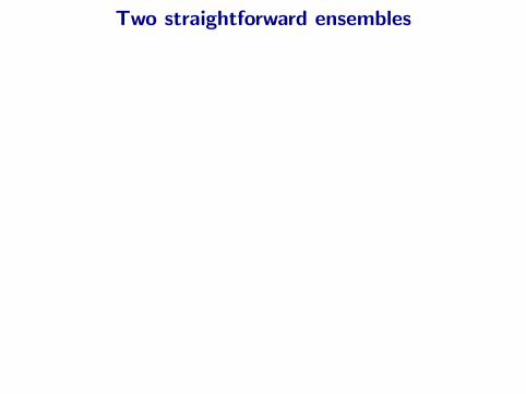
Summary and open questions
Practical method: ℓ1-regularized regression succeeds with sample size
n > c1 max d
θ2min
, d3 log p.
Martin Wainwright (UC Berkeley) High-dimensional graph selection August 2009 26 / 27
Summary and open questions
Practical method: ℓ1-regularized regression succeeds with sample size
n > c1 max d
θ2min
, d3 log p.
Fundamental limit: any algorithm fails for sample size
n < c2 max 1
θ2min
, d2 log p
various open questions: determine exact capacity of problem (including d2 versus d3 and control of
constants)
Martin Wainwright (UC Berkeley) High-dimensional graph selection August 2009 26 / 27

Summary and open questions
Practical method: ℓ1-regularized regression succeeds with sample size
n > c1 max d
θ2min
, d3 log p.
Fundamental limit: any algorithm fails for sample size
n < c2 max 1
θ2min
, d2 log p
various open questions: determine exact capacity of problem (including d2 versus d3 and control of
constants)
some extensions....⋆ non-binary MRFs via block-structured regularization schemes⋆ other performance metrics (e.g, (1 − δ) edges correct)
broader issue: optimal trade-offs between statistical/computationalefficiency?
Martin Wainwright (UC Berkeley) High-dimensional graph selection August 2009 26 / 27

Some papers on graph selection
Ravikumar, P., Wainwright, M. J. and Lafferty, J. (2008).High-dimensional Ising model selection using ℓ1-regularized logisticregression. Appeared at NIPS Conference (2006); To appear in Annals ofStatistics.
Ravikumar, P., Wainwright, M. J., Raskutti, G. and Yu, B.High-dimensional covariance estimation: Convergence rates ofℓ1-regularized log-determinant divergence. Appeared at NIPS Conference2008.
Santhanam, P. and Wainwright, M. J. (2008). Information-theoreticlimitations of high-dimensional graphical model selection. Presented atInternational Symposium on Information Theory, 2008.
Wainwright, M. J. (2009). Sharp thresholds for noisy andhigh-dimensional recovery of sparsity using ℓ1-constrained quadraticprogramming. IEEE Trans. on Information Theory, May 2009.
Martin Wainwright (UC Berkeley) High-dimensional graph selection August 2009 27 / 27
Related Documents

![Netplexity - the complexity of interactions in the real … · Netplexity The Complexity of Interactions in the ... Douglas Adams] Complexity and ... –Mathematical graph theory](https://static.cupdf.com/doc/110x72/5b89f5367f8b9a9b7c8b4a01/netplexity-the-complexity-of-interactions-in-the-real-netplexity-the-complexity.jpg)