On the rheology of shear-thickening and magnetorheological fluids under strong confinement TESIS DOCTORAL Programa de Doctorado en Física y Ciencias del Espacio Elisa María Ortigosa Moya Directores Juan de Vicente Álvarez-Manzaneda Roque Isidro Hidalgo Álvarez Grupo de Física de Fluidos y Biocoloides Departamento de Física Aplicada 2020

Welcome message from author
This document is posted to help you gain knowledge. Please leave a comment to let me know what you think about it! Share it to your friends and learn new things together.
Transcript
On the rheology of shear-thickening
and magnetorheological fluids
under strong confinement
TESIS DOCTORAL
Programa de Doctorado en Física y Ciencias del Espacio
Elisa María Ortigosa Moya
Directores
Juan de Vicente Álvarez-Manzaneda
Roque Isidro Hidalgo Álvarez
Grupo de Física de Fluidos y Biocoloides
Departamento de Física Aplicada
2020

Editor: Universidad de Granada. Tesis Doctorales Autor: Elisa María Ortigosa Moya
ISBN: 978-84-1306-706-3 URI: http://hdl.handle.net/10481/65310

A mis padres y mi hermana.
A los hijos de la tierra
y los peces de ciudad.

vii
Agradecimientos
Llega el momento de dedicar unas líneas de agradecimiento sincero a todos
aquellos que de una u otra manera han estado a mi lado en días de sol, nubes
y lluvia, ofreciéndome su ayuda, apoyo y tiempo para llevar a buen término
esta tesis.
En primer lugar quiero comenzar por dar las gracias a mis directores de
tesis. A Juan, por ofrecerme la posibilidad de trabajar junto a él, un excepcio-
nal investigador con capacidad para guiar el trabajo de cada vez más gente y
hacerlo bien, además. Y a Roque, un insaciable aprendiz que contagia su ilu-
sión por la ciencia. Gracias por lo aprendido y por vuestra confianza, consejos
y paciencia durante estos años.
Gracias también a los miembros del Departamento de Física Aplicada, en
especial al Grupo de Física de Fluidos y Biocoloides, por dejarme aprender de
vosotros en cada seminario y ayudarme en lo que he necesitado: Ana Belén,
Julia, Alberto, Arturo, Teresa, Wagner, Curro y Miguel Ángel. A María, por su
disposición y su sonrisa imborrable; a Pepe, compañero en el sótano con
quien habría disfrutado en clase como alumna; a Delfi por sus firmas y cariño;
a Miguel Cabrerizo, por acercar la ciencia a la gente; y especialmente a María
José, Fernando y Stefania, por su constante ayuda en las prácticas de Biofísica
cada curso. Del mismo modo, también ha sido un placer compartir las prácti-
cas de Fundamentos físicos aplicados a las estructuras con Artur, Javier, Enri-
Agradecimientos
viii
que, Matilde, José Antonio y Jorge, que tantas veces ha bajado las escaleras
para asegurarse de que todo funcionaba bien en la sala. También quiero agra-
decer la labor de los administrativos Conrado, Belén y Raquel, y la de Ángel y
María Jesús como coordinadores del programa de doctorado, por su amable
trato y facilitarnos la burocracia. Así mismo también me acuerdo de Felisa y
su preciosa Ángela, de Marisa y esa coreografía tan ensayada y de María del
Mar, que no dejó de repartir abrazos, alegría y sororidad.
Este tiempo habría sido muy distinto de no ser por mis compañeros de la
sala 𝜋𝑓, gracias a todos ellos por compartir tantos momentos juntos. A aque-
llos que estuvieron poco tiempo al principio pero que sembraron un ambiente
estupendo: Juan Pablo, Azahara, Germán y Diego. A José Antonio, por su sim-
patía e inestimable ayuda en mis innumerables tropiezos con las simulacio-
nes. Al hijo adoptivo de Nerja, Keshvad, por enseñarme tribología y encontrar
los dulces más ricos en cada aeropuerto. A José Rafael, un ejemplo de eficien-
cia que ha superado cada rasguño del rugby. Al fascinante y aventurero Guille,
que nos llevó en chanclas hasta el techo peninsular y no dejó de alentarnos
por aquellos preciosos parajes. A Tamara, por traer orden al laboratorio y una
nueva sonrisa a la sala. A los que estuvieron de paso menos tiempo, como Ma-
ría Laura con sus palabras de ánimo, antiguas y recientes, para “meterle pila”
a la tesis; la encantadora Camila, Ester, Mónica, Ángel, Blanca, Alan, Jianjian,
Martin y Dorota. Gracias también a Pablo Ibáñez, Yan, Alicia, Matthew, Pablo
Graván y Sara por reavivar la sala, espero que sigáis cuidando de ella.
Quiero dar las gracias a Paloma, Pablo y Samuel por luchar por todos, y a
Milagros por su cercanía y apoyo. A Jose y Santiago, por solucionar problemi-
llas en los clusters Proteus y Alhambra y su disposición a ayudarme cuando lo
he necesitado. A los compis de la peña, con los que recargué las pilas cada
miércoles. A Aurora, por su fiel compañía carrera tras carrera y hacerse un
hueco entre nosotros. A Matt y David, por acompañarnos siempre que han
podido. Y también a Maxwell, del que cada vez me asusto menos aunque salte
más, y a Pablo Pamplona, Oviedo, Zamora…, por las divertidas confusiones.
Recorrer el largo y pedregoso camino que emprendí ha sido mucho más
fácil dentro de una burbuja rebosante de calidad humana, comprensión, com-
pañía, entretenimiento, comida (mucha) y, en definitiva, amistad. Gracias por
dejarme crecer y aprender a vuestro lado. A la divertida y organizada Irene,
que tanto me ha hecho reír y enseñado sobre la idiosincrasia granaína. Es im-
posible no echarla de menos a mi espalda, en el fútbol o bailando con lenguaje
de signos. Menos mal que aun sin estar sigue estando y deleitándonos con sus
Agradecimientos
ix
peripecias y virtuosismo eligiendo GIFs. A la pizpireta Aixa, por esas recetas
tan ricas que nos ha preparado durante este tiempo y contagiarnos su alegría.
A Luis, por estar pendiente de mí en los momentos delicados, ser un buen
senpai y entretenernos con sus aventuras. Gracias Leo, por ser el pegamento
más antiguo y duradero del grupo, cuidar de todos nosotros y enseñarnos a
compartir. A Migue, que casi no tuvo cascarón y de quien tanto se puede
aprender. A Pablo con su desparpajo malagueño y su faceta actoral, porque
todo es más divertido si está cerca. A Nico, por su energía desbordante y su
memoria infinita para el quesito rosa, lleno de ideas para hacer regalos de
tesis y sobre dónde ir a comer, y por presentarme a los dragones. A Ana, que
no puede ser más “apañá”, por los ratos de recetas, costura, deporte y los cur-
sillos exprés de sevillanas. A Javi con sus apuestas siempre ganadoras, por
enseñarme algo de fonética y por qué el 28 es un número perfecto, aunque
nunca viéramos su tesis. A su particular Zipi, Alvaro, por sus acertadas reco-
mendaciones tecnológicas. El brillante Adri consiguió que muchos nos leyé-
ramos su tesis para encontrar dónde estaba la gracia, al mismo tiempo que
nos recordaba que somos una ohana en la que nadie se deja atrás. Gracias al
polifacético José Alberto, por aguantarme estos años y cuidar de mí, por ense-
ñarnos a protegernos para ser un poquito más libres, por las clases de armo-
nía y mostrarme unos anillos muy lejanos, por tantas risas y complicidad. Soy
muy consciente de que difícilmente volveré a toparme con tanta gente tan
capaz, divertida y cariñosa como vosotros. Sois especiales.
También quiero dar las gracias a mis ingenieros repartidos por el mundo,
por su memoria, con la que completamos nuestros puzles de anécdotas pasa-
das para acabar llorando de risa: Nuria, Susana, Blanco, Juanjo, Antonio,
Abraham, Candela y mis queridos tomatitos. También quiero agradecer su
continuo interés y apoyo a Amabel, Lorena, Dani y Alfonso.
A Pedro, que me peina el alma y me la enreda, y cuyo aliento y sustento
no me dejan caer. Gracias por seguir estando a mi lado por lejos que me en-
cuentre, por hacerme reír y mimarme, por quererme. A mi familia, que siem-
pre está ahí aunque todo cambie, y a la dulce Rocío. A mi hermana, Jose y sus
dos tesoros, que consiguen sacarme una sonrisa a la mínima. Y, finalmente,
gracias a mis padres, los cimientos firmes que siempre me ofrecen su ejemplo
de lucha, unión y amor, y que me enseñaron que ante un gran salto como este
hay que coger un gran impulso. Os quiero.

xi
Financiación
La investigación que ha conducido a la realización de esta tesis doctoral
ha sido financiada por el Ministerio de Economía y Competitividad
(MINECO), mediante los proyectos MAT 2013-44429-R y MAT 2016-
78778-R, el Fondo Europeo de Desarrollo Regional (FEDER) y por la Jun-
ta de Andalucía mediante el proyecto P11-FQM-7074. La doctoranda
agradece la ayuda predoctoral para la formación de doctores FPI
2014/069341.

xiii
Contents
Abstract
Resumen
Part I: Introduction
xvii
xxi
1
1. Background 3
1.1. Complex fluids 3 1.1.1. Colloids 4 1.1.2. Field-responsive materials 7 1.1.3. Concentrated suspensions 11 1.1.4. Shear thickening 12
1.2. Basis on magnetism 14 1.2.1. Types of magnetic materials 16
1.3. Rheology 17 1.3.1. Types of materials and their rheological response 18 1.3.2. Constitutive equations and material functions 20 1.3.3. Effect of volume fraction in viscosity 24
1.4. Tribology 26 1.4.1. Generalities 26 1.4.2. Reynolds equation 31 1.4.3. Film thickness 32
1.5. Simulation methods for colloidal suspensions 35 1.6. References 36
Contents
xiv
2. Justification 41
2.1. Objectives 43 2.2. Outline of the thesis 44
2.2.1. Rheology in dense suspensions 44 2.2.2. Tribology in inelastic non-Newtonian fluids 45 2.2.3. Rheology of diluted MR fluids under squeeze flow 46
3. Methodology 47
3.1. Materials 47 3.1.1. Starch 47 3.1.2. Fumed silica 50 3.1.3. Carbonyl iron 50 3.1.4. Sample preparation 52
3.2. Experimental methods 56 3.2.1. Rheometry 56 3.2.2. Tribometry 67 3.2.3. Microscopic characterization 68 3.2.4. Analysis of particle size distribution 73 3.2.5. Colloidal stability 75 3.2.6. Contact angle measurement 80 3.2.7. Calibration of the magnetic field applied by a solenoid 81
3.3. Simulation methods 82 3.3.1. Interactions in particle-level dynamic simulations 82 3.3.2. Simulation of mixtures of particles 93 3.3.3. Squeeze simulations 96 3.3.4. EHL simulations 97
3.4. References 104
Part II: Results and discussion 111
4. Shear thickening in unimodal suspensions 113
4.1. Introduction 113 4.2. Materials and methods 116
4.2.1. Materials 116 4.2.2. Rheometry 118
4.3. Results and discussion 119 4.3.1. Starch and fumed silica-based suspensions 119 4.3.2. Carbonyl iron-based suspensions 124
4.4. Conclusions 131 4.5. Supplementary material 133 4.6. References 134
Contents
xv
5. Shear thickening in bimodal suspensions 139
5.1. Introduction 139 5.2. Experimental 143
5.2.1. Materials 143 5.2.2. Rheometry 144 5.2.3. Coating of carbonyl iron particles 145
5.3. Simulation method 147 5.4. Results and discussion 150
5.4.1. Bimodal MRST suspensions 150 5.4.2. Suspensions of hybrid core-shell particles 159 5.4.3. Comparison between bimodal suspensions and formulated with hybrid core-shell particles 164 5.4.4. Simulation of mixtures of monodisperse particles 165 5.4.5. Simulation of mixtures of polydisperse particles 173
5.5. Conclusions 178 5.6. References 180
6. Isoviscous elastohydrodynamic lubrication of inelastic non-Newtonian fluids 187
6.1. Introduction 188 6.2. Experimental and simulations 190 6.3. Results and discussion 193
6.3.1. Simplified solution approach 193 6.3.2. Full solution approach 194
6.4. Conclusions 206 6.5. References 207
7. Soft lubrication of cornstarch-based shear-thickening fluids 211
7.1. Introduction 212 7.2. Experimental and simulations 214 7.3. Results and discussion 217
7.3.1. Rheological characterization 217 7.3.2. Tribological characterization 219 7.3.3. Effect of starch concentration 224 7.3.4. Comparison between experiments and numerical simulations 227
7.4. Conclusions 228 7.5. Supplementary material 230 7.6. References 231
8. On the squeeze-strengthening effect in magnetorheology 237
8.1. Introduction 237
Contents
xvi
8.2. Materials and Methods 240 8.2.1. Materials 240 8.2.2. Rheological tests 240
8.3. Theory 242 8.4. Squeeze simulations 244 8.5. Results and Discussion 246
8.5.1. Squeeze flow behaviour of MR fluids 246 8.5.2. Steady shear flow of compressed MR fluids 249 8.5.3. Effect of the densification process in constant-area experiments 250 8.5.4. Influence of the carrier fluid in the compression behaviour of MR fluids in constant-volume tests 252 8.5.5. Importance of the field gradient in the compression behaviour of MR fluids in constant-volume tests 254 8.5.6. Simulations for constant-volume and constant-area conditions 255
8.6. Conclusions 257 8.7. References 258
Part III: Conclusions 263
9. Conclusions 265
xvii
Abstract
Suspension rheology is capturing a great interest in recent years due to the
importance of complex suspensions in multitude of industrial applications.
Among them, shear-thickening (ST) and magnetorheological (MR) fluids are
very valuable materials for their ability of readily tuning their rheological be-
haviour, well passively by shear or actively in presence of external fields, re-
spectively. Both complex fluids are used in energy dissipating systems: ST
fluids are mainly used as impact-resistant materials or shock absorbers in
protective applications, while MR fluids are extensively employed in torque
transfer applications.
The counter-intuitive phenomenon of shear thickening displays a re-
versible increase in viscosity (continuous or discontinuous) under applied
shear rates or stresses. For this non-Newtonian behaviour to occur it is nec-
essary to reach a critical volume fraction and shear rate, in systems where
attraction is negligible. These shear-thickening features can be controlled by
means of several strategies, such us changing some particle or fluid proper-
ties during the formulation of these complex fluids, or introducing net attrac-
tive forces. Nowadays scientific community broadly agrees that ST is due to a
transition from a hydrodynamically lubricated regime to a friction dominated
situation, especially in dense systems. It is in close contact conditions where
the fields of rheology and tribology are connected, as the local friction deter-
Abstract
xviii
mines the microstructure that give rise to certain macroscopic rheological
response.
On the other hand, as it happens in the case of ST fluids, the rheological
properties of MR fluids can also be varied, but by the action of an external
magnetic field. They are suspensions of magnetic micronsized particles sus-
pended in a non-magnetic Newtonian fluid. When subjected to an external
magnetic field these particles become polarized and aggregate in chains or
columnar structures that orientate along magnetic field lines. As a result of
this field-induced assembly, the suspension experiences a reversible liquid-
to-solid transition, as the viscosity of MR fluids rapidly increases several or-
ders of magnitude, what is known as magnetorheological effect, and it is occa-
sionally accompanied by a yield stress. Magnetorheological applications have
to deal with some drawbacks due to particle sedimentation, which is general-
ly improved by the incorporation of additives into the carrier in order to re-
duce the density mismatch between particles and carrier.
The meeting point between ST and MR systems are magnetorheological
shear-thickening (MRST) suspensions, i.e., concentrated hybrid systems
whose rheological behaviour can be easily tuned, well passively with a given
flow deformation or actively through an applied magnetic field strength.
These suspensions are still scarcely studied and, apart from controlling the
appearance and intensity of the shear thickening behaviour, it has been
shown that the partial substitution of magnetic particles by non-magnetic
ones in MR fluids produces an increase in yield stress.
Besides, the operational mode also affects the MR fluid performance. In
this sense, it has been demonstrated a yield stress enhancement when the MR
fluid with certain concentration is subjected to slow compression prior to a
shear flow mode under the application of an external field, the so-called
squeeze strengthening effect.
Having said that, the research works presented in this dissertation can be
classified in three main topics: rheology of concentrated suspensions that
show shear-thickening and/or magnetic response, tribology of non-
Newtonian fluids, and squeeze-strengthening effect under constant-volume
and constant-area conditions. These three matters were studied experimen-
tally and by simulations. Regarding the first topic, we investigated shear-
thickening in dense suspensions formulated with one and two types of parti-
cles, magnetic and non-magnetic ones, and explore the effect of the type of
Abstract
xix
particle, concentration, carrier fluid and magnetic field. Particle-level dynamic
simulations were performed in both monodisperse and polydisperse mix-
tures of particles in order to reproduce shear-thickening behaviour and the
enhancement in yield stress due to partial substitution of magnetic particles
in MR fluids. With respect to the second topic we studied tribological behav-
iour of non-Newtonian fluids, both shear-thinning and shear-thickening flu-
ids, in the elastohydrodynamic regime. Numerical simulations try to repro-
duce the pressure distribution, film thickness and frictional properties of
these fluids within this regime, and a master curved is proposed and evaluat-
ed with experimental results. Concerning the last topic, we investigated the
slow compression of diluted MR fluids subjected to an external magnetic field,
under constant-volume and constant-area conditions. We highlight that high-
er yield stresses found in constant-area compared to constant-volume condi-
tions, are due to the effect of the densification occurring during the compres-
sion of the fluid in the constant-area case. Particle-level simulations mimicked
the compression and shear processes and also showed higher yield stresses
in constant-area compression.

xxi
Resumen
En los últimos años, la reología de suspensiones está captando un gran interés
por su importancia en multitud de aplicaciones industriales. Entre ellas, los
fluidos espesantes y magnetorreológicos son materiales muy apreciados por
su capacidad de modificar su comportamiento reológico fácilmente, bien sea
de pasivamente al someterlos a cizalla o de forma activa en presencia de
campos externos, respectivamente. Ambos fluidos complejos se utilizan en
sistemas de disipación de energía: los fluidos espesantes su usan principal-
mente en aplicaciones de absorción de impactos, mientras que los fluidos MR
se emplean ampliamente en aplicaciones que requieren transferencia de par.
El comportamiento espesante en condiciones de cizalla es un fenómeno
contrario a la intuición, ya que muestra un aumento reversible de la viscosi-
dad (continuo o discontinuo) con la velocidad de deformación o el esfuerzo
aplicados. Para que este comportamiento no newtoniano tenga lugar es nece-
sario alcanzar valores críticos de fracción de volumen y velocidad de defor-
mación, en sistemas en los que la atracción es insignificante. Las característi-
cas del perfil de espesamiento pueden controlarse mediante varias estrate-
gias, como la modificación en las propiedades de las partículas o los fluidos
portadores durante la formulación de estas suspensiones complejas, o la in-
troducción de fuerzas atractivas. Hoy en día la comunidad científica coincide
ampliamente en que el origen del comportamiento espesante en sistemas
Resumen
xxii
concentrados se debe a la transición desde un régimen lubricado hidrodiná-
micamente hasta una situación dominada por la fricción. En condiciones de
estrecho contacto confluyen los campos de la reología y la tribología, ya que la
fricción local entre partículas determina la microestructura que da lugar a
una determinada respuesta reológica macroscópica.
Por otro lado, las propiedades reológicas de los fluidos MR también pue-
den modificarse, como sucede con los fluidos espesantes, pero por la acción
de un campo magnético externo. Estos fluidos son suspensiones de partículas
magnéticas de tamaño micrométrico suspendidas en un fluido newtoniano no
magnético. Cuando se someten a un campo magnético externo, estas partícu-
las se polarizan y se agregan en cadenas o estructuras columnares que se
orientan a lo largo de las líneas de campo magnético. Como resultado de este
ensamblaje inducido por el campo, la suspensión experimenta una transición
reversible de líquido a sólido, como consecuencia de un aumento muy rápido
en la viscosidad del fluido, de varios órdenes de magnitud. Esto se conoce co-
mo efecto magnetorreológico, y ocasionalmente va acompañado de un esfuer-
zo umbral. Las aplicaciones de estos fluidos requieren acciones que mitiguen
la sedimentación de partículas, generalmente ésta se mejora mediante la in-
corporación de aditivos en el fluido portador y así reducir el desequilibrio
entre partículas y líquido.
El punto de encuentro entre los sistemas espesantes y los fluidos MR son
las suspensiones espesantes magnetorreológicas (MRST). Se trata de sistemas
híbridos concentrados cuyo comportamiento reológico se puede ajustar fá-
cilmente, bien de forma pasiva con una determinada deformación de flujo o
de forma activa a mediante la aplicación de un campo magnético. Estas sus-
pensiones que combinan tanto el comportamiento espesante como el magné-
tico han sido foco de algunas investigaciones, pero han sido poco estudiadas.
Aparte de controlar la aparición e intensidad del espesamiento debido a la
cizalla, se ha demostrado que la sustitución parcial de las partículas magnéti-
cas por otras no magnéticas en los fluidos MR produce un aumento del es-
fuerzo umbral.
Además, el tipo de flujo al que se someten los fluidos MR afecta a su com-
portamiento reológico. En este sentido, se ha demostrado un aumento del es-
fuerzo umbral cuando el fluido MR con una cierta concentración se somete a
una compresión lenta previa al flujo de cizalla, en condiciones de campo apli-
cado. Este efecto se debe a una recolocación de las partículas magnéticas que
Resumen
xxiii
forman las cadenas, como consecuencia de la compresión, y que da lugar al
refuerzo de estas estructuras.
Dicho esto, los trabajos de investigación presentados en esta tesis pueden
clasificarse en torno a tres temas principales: reología de suspensiones con-
centradas que muestran un espesamiento en flujo de cizalla y/o respuesta
magnética, tribología de los fluidos no newtonianos y comportamiento de
fluidos MR sometidos a compresión lenta en condiciones de volumen y área
constantes. Estas tres materias se han abordado tanto experimentalmente
como mediante simulaciones. En cuanto al primer tema, investigamos el es-
pesamiento en suspensiones concentradas formuladas con uno y dos tipos de
partículas, tanto magnéticas y como no magnéticas, y exploramos el efecto del
tipo de partícula, la concentración, el fluido portador y el campo magnético.
Se realizaron simulaciones dinámicas a nivel de partícula en mezclas de partí-
culas monodispersas y polidispersas, con el fin de reproducir el comporta-
miento espesante y el aumento del esfuerzo umbral provocado por la sustitu-
ción parcial de las partículas magnéticas en los fluidos MR. Con respecto al
segundo tema, se estudió el comportamiento tribológico de fluidos no newto-
nianos, tanto fluidos espesantes como fluidificantes, en el régimen de lubrica-
ción elastohidrodinámica. Las simulaciones numéricas realizadas pretenden
reproducir la distribución de la presión, el espesor de la película y las propie-
dades de fricción de estos fluidos dentro de este régimen, y se ha propuesto
una expresión para la curva maestra, que ha sido validada con los. En cuanto
al último tema, investigamos la compresión lenta de los fluidos diluidos de
MR sometidos a un campo magnético externo, bajo condiciones de volumen y
área constantes. Destacamos la obtención de mayores esfuerzos umbrales en
compresiones a área constante con respecto a los experimentos realizados a
volumen constante, y que son consecuencia del aumento de la fracción de vo-
lumen entre los platos a medida que la compresión avanza. Se han usado nue-
vamente simulaciones a nivel de partícula que replican los flujos de compre-
sión y cizalla experimentales, y también mostraron mayores esfuerzos um-
brales en compresión en área constante.


I Introduction

3
1. Background
Complex fluids 1.1.
The mechanical behaviour of matter can be classified basically in two catego-
ries: solid and fluid. However most materials belong to a grayscale between
these two cases and present intermediate characteristics between these lim-
its, so that this binary classification is insufficient [1]. It is the case of soft mat-
ter and complex fluids [2]. This kind of materials self-organizes in mesoscopic
structures that provide a partial order. Interactions between these entities
are generally weak and comparable with thermal energy, what contribute to
some of their features, as an easy deformability and sensitivity to thermal
fluctuations and other external actions [3,4]. Soft matter is ubiquitous both in
nature and in industrial applications. Examples of soft materials include,
among others, polymers, colloids, liquid crystals, biological matter or granular
materials, and are applied in fields like food, personal care products, paints
and cements.
These systems may occasionally display a particularly complex and coun-
ter-intuitive behaviour, even at room temperature. The subset of soft matter
that can flow but exhibit non-Newtonian rheology is called complex fluids.
These structured multicomponent systems are known by some of their defin-
ing adjectives as smart, tuneable or responsive materials, because of their
1. Background
4
ease in changing some properties under a given external stimuli, such as
stress, temperature, light or magnetic field.
In relation to the supramolecular assembling characterizing soft matter,
Pierre Gilles de Gennes received the Nobel Prize in Physics (1991) “for dis-
covering that methods developed for studying order phenomena in simple
systems can be generalized to more complex forms of matter, in particular to
liquid crystals and polymers”. He is considered the father of this broad disci-
pline that covers from the vulcanisation of rubber to the lather of a shampoo
[5]. He compared this fragile and deformable matter with the clay of a sculp-
tor, as its malleability allows for a delicate adjustment upon the subtle action
of the artist’s hand.
Colloids 1.1.1.
Colloids are dispersed systems composed by mixtures of one or more dis-
persed phases homogeneously distributed in a continuous medium. The par-
ticle size of the colloidal range goes from 1 nm to 1 μm. Systems with particles
in this range are known as dispersions (average diameter being 100 nm),
while in the case of having larger particles, the colloidal system is called sus-
pension. In colloidal science the suspending medium is considered a continu-
um, and the lower limit of the colloidal range guarantee that particles are
larger than the carrier molecules. Below this limit both particles and mole-
cules of the suspended fluid are indistinguishable, so that we would be talking
about solutions, with a unique phase. On the other hand, the upper limit seeks
to ensure negligible sedimentation and still significant thermal forces in the
motion of colloidal particles. Sedimentation can occur when particles are
above 1 μm (Brownian motion becomes negligible) or have high density.
These composed systems are mainly characterized by high particle diffu-
sion coefficient, slow sedimentation under normal gravity, showing weak
light scattering, and suspension structuring. Due to the fineness of particles
(i.e., large specific surface area), surface area properties of the dispersed
phase and their physico-chemical interaction with the solvent are properties
of great importance in colloidal science. Other interesting features comprise
the particle morphology, concentration and suspension properties (such as
turbidity, viscosity and stability), among others [6].
Colloidal particles are not necessarily solids neither the carrier fluid a
liquid. Depending on the state of the matter of both dispersed phase and dis-
persion medium, several types of colloids are found: foams, aerosols, emul-
1.1. Complex fluids
5
sions, gels, sols. Typical examples of colloids in daily life are inks, milk, blood,
gelatine, whipped cream, fog and atmospheric particulate matter [7].
The kinetic stability or colloidal stability of these systems depends on the
forces the particles are subjected to. In this sense, the macroscopic behaviour
of the whole suspension relies on the nature of microscopic interactions be-
tween colloidal particles.
A single colloidal particle suspended within the carrier fluid is subjected
do three forces: Brownian, hydrodynamic and gravitational forces. In general,
the order of magnitude of these forces (O(1015 N)) is similar for colloidal-
sized particles.
- Small particles dispersed in a medium are always subjected to
Brownian motion, which randomly moves the particles due to the
thermal fluctuations and collisions with the fluid molecules.
- Hydrodynamic force is due to the particle drag (Stokes) because of
being immersed within the carrier fluid.
- Gravitational forces give rise to particle sedimentation, which can be
avoided by equalizing the densities of each phase.
Colloidal interactions [6] refer to particle-particle interactions through
the fluid, and three types can be distinguished: dispersion, surface, and hy-
drodynamic forces. These interactions depend on the chemical and material
properties of the particles and can be attractive or repulsive.
- Surface forces are short-range forces that arise when particles are
close enough: electrostatic interaction is generally repulsive and is
due to electrical charge often carried by colloidal particles on their
surfaces and properties of the continuous phase; repulsive steric
forces (or excluded volume), usually generated when particles are
covered with grafted polymers or surfactants; and attractive deple-
tion forces that exclude smaller solutes (non-adsorbed polymers)
from the vicinity of large colloidal particles.
- Dispersion forces, such as the attractive and short-range van der
Waals forces, appear when atoms in a given colloid induce polariza-
tion in other colloid nearby.
- The last comes from the disturbance in the flow produced by the
presence of other particles.
1. Background
6
The linear addition of the attractive diffusion potential and the electro-
static repulsive potential is known as Derjaguin-Landau-Verwey-Overbeek
(DLVO) theory [8–11] and is used satisfactorily to explain stabilization. Gen-
erally, the total interaction energy as a function of the distance between parti-
cle surfaces presents two local minima and one local maximum. Van der
Waals attraction give rise to the first primary minimum at small surface dis-
tances, as adhesion of particles is an energetically favourable process. At larg-
er surface distances, if van der Waals interactions are strong and repulsion
from the double layer interactions play a significant role, the second mini-
mum appears as well as the local energy maximum. This means that coagula-
tion is produced when decreasing the electrostatic repulsive forces and when
particles are forced to be in close proximity. At great distances there will not
be any interactions between identical colloidal particles.
Besides previous interactions, other short-range repulsive interaction
may be observed, particularly for hydrophilic surfaces in polar solvents, the
so-called solvation or hydration interaction.
Particles will aggregate if attractive forces dominate, while when repul-
sive forces prevail, the colloidal system remains stable. For the sake of clarity,
in this case we refer to microscopic stability (absence of particle aggregation)
and not to the less used macroscopic stability (constant and homogeneous
distribution of the dispersed phase). Aggregation and sedimentation are the
main phenomena involved in the destabilization of the colloidal system.
Therefore, the minimization of particle aggregation requires the enhance-
ment of repulsive interaction forces, through electrostatic and steric stabiliza-
tion. Regarding particle sedimentation it can be improved by reducing the
density mismatch between the carrier fluid and the dispersed phase. Poly-
mers are broadly used for this function as they are able to form a gel matrix
that complicates the normal particle motion. Moreover, polymeric chains also
hinder particle aggregation as impede them to be closer.
Colloidal stability can be enhanced through changes in the viscosity, acid-
ity, ionic concentration or addition of some component, such a surfactants or
polymers to the suspending fluid. It is interesting that the use of additives to
improve the stability was already employed by ancient Egyptians, when they
added Arabic gum to impede flocculation of carbon black particles in the
preparation of inks [5]. In this case, the explanation of the stabilization of the
colloidal suspension of carbon black comes from the fact that grains of carbon
black were coated by hydrophilic polymers whose bonds with water mole-
1.1. Complex fluids
7
cules were stronger than van der Waals attractions between the macromole-
cules.
Field-responsive materials 1.1.2.
Field-responsive fluids have attracted much attention during last century due
to the ease in changing and controlling material properties upon the applica-
tion of an external stimulus, namely electric or magnetic fields. Electrorheo-
logical (ER) fluids and magnetorheological (MR) suspensions [12] belong to
this subclass of smart materials, as well as magnetic colloids and other mag-
netic hybrid systems with solid matrices.
The discovery of ER and MR fluids occurred almost simultaneously. On
the one hand, in 1948 Jacob Rabinow [13] designed several devices at the US
National Bureau of Standards in which an iron-oil mixture became almost sol-
id when subjected to a magnetic field; it was the origin of a new type of mag-
netic fluids, i.e., MR fluids. For its part, Willis M. Winslow reported the ER ef-
fect also in the 1940s [14]. ER fluids are the electric analogous of MR fluids,
and consist of electrical polarizable particles (silica, titania, zeolites) dis-
persed in a carrier fluid (silicone oil, mineral oil). Similarly to MR fluids, un-
der the influence of an electric field they dramatically modify their rheological
properties. Both field-responsive fluids respond to an external field exhibiting
a reversible and fast transition from liquid to solid state as a consequence of
the dipole-dipole interactions between the constituent particles. The appar-
ent viscosity can show an increase of several orders of magnitude from the
off-state to the on-state, which can be easily tuned by controlling the external
field. Other difference is the maximum yield strength obtained in ER fluids,
which is much lower than that found in MR fluid. This affects the mechanical
applicability of each type of fluid as well as the size of the required device.
Because of the stronger field-induced interactions in MR fluids, they are usu-
ally preferred over ER fluids. One of the focuses during this thesis is the study
of magnetorheological fluids under certain flow conditions.
Apart from MR fluids, other types of magnetic fluids structure under the
action of a magnetic field giving rise to changes in their properties [15]. They
can be classified according to their magnetizable phase. If the solid phase is
magnetic we can talk about ferrofluids (FF) [16] and magnetorheological flu-
ids (MRF) [17,18]. In inverse ferrofluids (IFF) instead it is the carrier fluid
that provides the magnetic response [19,20]. Some of the main characteristics
of these magnetic fluids are exposed below.
1. Background
8
Magnetorheological fluids
A typical MR fluid is generally formulated with magnetic soft particles (e.g.,
carbonyl iron) suspended at high concentration in mineral oils, aqueous solu-
tions, etc. In this case particle size ranges from tens of nanometers to tens of
micrometers. Above a critical value in particle size they possess magnetic
multidomains. In the absence of magnetic field this fluid acts as a convention-
al suspension as the net dipole is very small. When subjected to magnetic
field, Bloch walls gradually shift in the sense of increasing the magnitude of
the magnetic moments oriented in the field direction and so the interparticle
interactions. Attractive interactions between particles result in columnar ag-
gregates that enhance the mechanical characteristics of the fluid. As a conse-
quence, the apparent viscosity of the fluid increases several orders of magni-
tude, what is known as magnetorheological effect, and it is occasionally ac-
companied by a yield stress. This increase produces a rapid and reversible
transition from liquid-like to solid-like state at sufficiently high fields, and can
be easily controlled by varying the magnetic field intensity. The maximum
effect depends on the saturation magnetization of the magnetic phase which
often shows magnetic remanence. In this sense, particles with a larger satura-
tion magnetization provide larger magnetic moments and thus larger MR ef-
fect.
Unlike the following magnetic fluid, particles in MR fluids may settle easi-
ly, due to the big particle size that hinders the occurrence of Brownian motion
and to the density difference between particles and fluid.
Ferrofluids
Ferrofluids were first formulated in the early 1960s by Steve Papell, an engi-
neer at Lewis Research Center (NASA), with the primary purpose of moving
the rocket fuel in no gravity conditions thanks to the magnetization of this
kind of magnetic liquid [21]. After that, Rosenzweig’s work improved the fab-
rication process, magnetization and stability of these fluids, and gave rise to
their industrial synthesis and commercialization. The fluid mechanics of these
magnetic fluids constitutes a branch of science is known a Ferrohydrodynam-
ics [22].
This stable colloidal magnetic fluid is composed of ferro- or ferrimagnetic
nanoparticles less than 10 nm in size (which is the typical size of
monodomains), usually magnetite, dispersed in polar or non-polar carriers.
These nanoparticles are frequently covered by some surfactant, in order to
1.1. Complex fluids
9
inhibit spontaneous coagulation. Due to the small particle size the particles
form individual magnetic domains, and Brownian motion due to thermal en-
ergy prevails over magnetic interaction, so that in absence of field the net
magnetization is null. Once the field is active particles orient in the direction
of the magnetic field. A remarkable difference with respect to MR fluids is that
FF always remains in fluid state in the presence of the field, and field-induced
structures that may develop a yield stress are not observed in this magnetic
fluid. Moreover, the small particle size provides a weaker magnetic response
compared to MR fluids. Therefore, unlike in MR fluids, their applications are
dictated for the fact of being magnetic fluids more than for the enhancement
in viscosity under an applied field.
Inverse ferrofluids
As previously commented, in IFF the magnetic response comes from the car-
rier fluid and not from the particles. The carrier is a ferrofluid with micromet-
ric and nonmagnetic particles dispersed in it. It can be seen somewhat as the
combination of MR fluids and FF. In IFF (or magnetic holes) interactions ap-
pear between particles even being non-magnetic, but as opposed to MR fluids,
the use of a FF as carrier provides a weak magnetic response. The major ad-
vantage compared to conventional MR fluids comes from the possibility of
selecting specific characteristics for the non-magnetic particles, as a given
morphology or a certain and controlled size.
Magnetorheological elastomers
Magnetorheological elastomers are obtained by dispersing micrometric-sized
magnetizable particles in a viscoelastic solid-like polymer gel or an elastomer.
Magnetic structures are formed if a uniform magnetic field is applied during
the cross-linking process, and these structures result retained within the ma-
trix. These materials are solid under all circumstances, their modulus or stiff-
ness can be varied by an applied field. The MR elastomers may find use in vi-
bration-control applications.
Apart from a particulate phase and a carrier, magnetic liquids may carry
certain additives, such as polymers and surfactants, that improve the formu-
lation as contribute to enhance the colloidal stability, reduce particle sedi-
mentation or prevent oxidation, which are the main drawbacks affecting their
durability and response in some applications. Unlike ER fluids where such
additives may decrease the ER effect, they have no influence on the polariza-
tion mechanism of MR fluids.
1. Background
10
Among the broad range of applications of magnetic fluids in everyday life
we will pay attention to those of ferrofluids and magnetorheological fluids as
they are the most widely used nowadays in industrial and biomedical applica-
tions.
Magnetic nanoparticles are receiving considerable attention due to their
potential application in drug delivery or hyperthermia treatment, and thus
ferrofluids formulated with them due to their magnetic control. For example,
in magnetic hyperthermia, a supplementary therapy in cancer treatments, a
combination of alternating magnetic fields and magnetic nanoparticles (a fer-
rofluid is injected) are used to heat specific tumour regions without damaging
other surrounding tissues. Magnetic nanoparticles are also employed in envi-
ronmental applications, such as in the removal of contaminants in water
treatment. These contaminants have high affinity for the specific functionali-
zation of particles, and the magnetic core allows for an easy recovery. Besides,
ferrofluids are employed in sealing and damping applications, with a remark-
able use as energy dissipating system in loudspeakers dampers.
Regarding MR fluids, an ideal magnetorheological device should enable
certain magnetic field with the least electrical power consumption and
weight. Moreover it should provide a significant response to the field (strong
MR effect), for which the selection of the involved phases and their interac-
tion become crucial. Some of the most common applications [15,23] are ex-
posed below.
- MR dampers are used to reduce vibrations by means of the dissipa-
tion of kinetic energy through the fluid. Those dampers are found in
shock absorbers, mounts, car and suspension, seismic protection in
buildings, cable stayed bridges or washing machines, among others.
- Torque-transfer applications such as in clutches, rotary brakes or hy-
draulic valves.
- Magnetic-circuits in which it is important to achieve an efficient pro-
duction and transmission of magnetic field.
- Manufacturing and process applications, such as the polishing and
finishing of optical components. In this application non-magnetic
abrasive particles are added to a MRF, and driven to the MR-
component interface under by applying a magnetic field.
1.1. Complex fluids
11
Concentrated suspensions 1.1.3.
Suspensions of non-colloidal particles are found in numerous applications in
industrial processes such in food processing or concrete, and in natural phe-
nomena such as slurries or lava. Due to the large particle size Brownian mo-
tion is neglected in these suspensions while the main interactions to be con-
sidered are hydrodynamic. However, interparticle forces depending on sur-
face interactions have to be taken into account only in the case of near con-
tact, it is, in concentrated suspensions.
Even if the carrier fluid is Newtonian (and without the influence of any
external field), the rheological behaviour of dense suspensions is nonlinear,
especially at high concentrations. Multi-body interactions in the system are
inevitable at large volume fractions so that apart of hydrodynamic interac-
tions through the liquid, frictional contacts become important due to the close
proximity the particles are subjected to. Therefore, the flow regime of dense
suspensions is intermediate between that of pure suspensions and granular
flow [24]. The description of the macroscopic behaviour of these complex
suspensions clearly depends on the microstructure formed as a consequence
of such interactions.
The addition of particles to a suspending Newtonian fluid with viscosity
휂𝑠 leads to an increase in its viscous dissipation and thus the deviation from
the Newtonian response. For example, at high particle concentration the sus-
pension may display an apparent yield stress, i.e., the fluid would only flow if
the applied stress overcomes this critical value. The increase in energy dissi-
pation comes from the friction of the particle surface with the fluid and from
the disturbance of the flow caused by the presence of particles. In this sense,
the increase in viscosity with particle concentration is higher when their
sphericity is decreased.
Among nonlinear and often unwanted effects that these concentrated
suspension can develop we usually encounter normal forces, shear-induced
migration, shear banding, sedimentation, thixotropy, aging, shear thickening
or jamming. For example, shear-induced migration appears when there are
spatial variations in shear rate so that particles migrate from high to low
shear regions, with the consequent concentration gradient and thus viscosity
gradient. Normal stresses for its part emerge as a consequence of the anisot-
ropy generated in the microstructure during shear. This variety of rheological
1. Background
12
behaviours depends on the shape, size and particle volume fractions and the
features of the applied deformation.
The dependence of the suspension viscosity 휂 as a function of the applied
shear rates or stresses gives rise to different rheological behaviours, ex-
plained in detail in the Subsection 1.3.2.
Shear thickening 1.1.4.
Shear thickening is a counter-intuitive phenomenon occurring in highly con-
centrated dispersions and suspensions, and it is characterized by a reversible
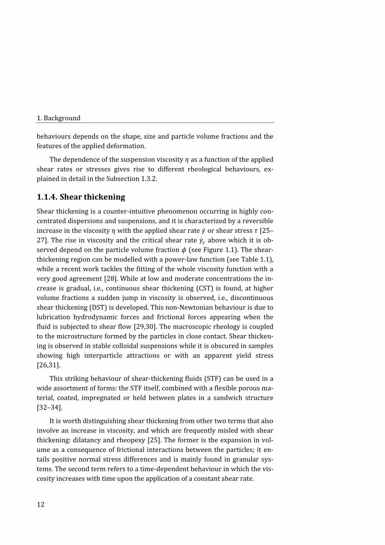
increase in the viscosity 휂 with the applied shear rate �̇� or shear stress 𝜏 [25–
27]. The rise in viscosity and the critical shear rate �̇�𝑐 above which it is ob-
served depend on the particle volume fraction 𝜙 (see Figure 1.1). The shear-
thickening region can be modelled with a power-law function (see Table 1.1),
while a recent work tackles the fitting of the whole viscosity function with a
very good agreement [28]. While at low and moderate concentrations the in-
crease is gradual, i.e., continuous shear thickening (CST) is found, at higher
volume fractions a sudden jump in viscosity is observed, i.e., discontinuous
shear thickening (DST) is developed. This non-Newtonian behaviour is due to
lubrication hydrodynamic forces and frictional forces appearing when the
fluid is subjected to shear flow [29,30]. The macroscopic rheology is coupled
to the microstructure formed by the particles in close contact. Shear thicken-
ing is observed in stable colloidal suspensions while it is obscured in samples
showing high interparticle attractions or with an apparent yield stress
[26,31].
This striking behaviour of shear-thickening fluids (STF) can be used in a
wide assortment of forms: the STF itself, combined with a flexible porous ma-
terial, coated, impregnated or held between plates in a sandwich structure
[32–34].
It is worth distinguishing shear thickening from other two terms that also
involve an increase in viscosity, and which are frequently misled with shear
thickening: dilatancy and rheopexy [25]. The former is the expansion in vol-
ume as a consequence of frictional interactions between the particles; it en-
tails positive normal stress differences and is mainly found in granular sys-
tems. The second term refers to a time-dependent behaviour in which the vis-
cosity increases with time upon the application of a constant shear rate.
1.1. Complex fluids
13
Figure 1.1: Schematics of the rheological behaviour of a concentrated suspension as a function of the volume fraction. The shear-thickening region appears at high shear rates, after shear-thinning and Newtonian regions. Significant shear-thickening parameters are
shown in the flow curve.
Different mechanisms have been proposed over the last decades to de-
scribe this unusual response to applied stresses occurring in densely packed
suspensions. In early works [35] shear thickening (mainly DST) was observed
together with dilatancy, and both concepts were used as synonyms. However,
dilatancy is just one of the necessary conditions to find the DST response.
Other mechanism developed by Hoffman [36,37] associated the DTS transi-
tion with an order-disorder transition. later, other scientists proposed the
formation of transient aggregates [38] as a consequence of the shear, labelled
hydroclusters, which are responsible for the viscosity increase. Hydrocluster
theory quantitatively agrees with the moderate increase in viscosity with the
shear rate (i.e., CST), but is insufficient to reproduce the large stresses found
during DST. In recent years, simulations have demonstrated that the use of
frictional forces along with hydrodynamic interactions adequately reproduce
DST curves as well as the transition from CST to DST when volume fraction
increases [29,39]. This demonstrates the intimate connection between rheo-
logical and tribological properties in densely-packed systems.
Systems developing this astonishing increase in the flow resistance and
energy dissipation are by far less known that shear-thinning materials, for
which the viscosity decreases with the shear rate. In spite of this peculiar re-
sponse to shear stresses or shear rates, it is interesting that one of the most
representative suspensions showing this behaviour is based on a widely-used
household product: cornstarch [40–43]. Dense suspensions of starch in water
1. Background
14
are perhaps the best known shear-thickening fluid exhibiting a dramatic in-
crease in viscosity when sheared or subjected to. It is fascinating how this be-
haviour arises from such a simple system and the fact that the main features
of shear thickening can be exhibited also by non-attractive hard spheres sus-
pended in a Newtonian liquid. This support the suggestion that shear thicken-
ing could be observed in all suspensions if the right conditions exist.
This thesis is primarily devoted to the study of dense cornstarch-based
suspensions and their rheological and tribological behaviour, as well as the
effect of adding magnetic particles to the systems to become thus in field con-
trolled suspensions.
Basis on magnetism 1.2.
Natural iron minerals found in the proximities of the ancient city of Magnesia
were the first mysterious stones in which magnetic phenomena were ob-
served, and their magnetic properties gave rise to the term magnetism.
Nowadays it is known that magnetic phenomena appears not only in
permanent magnets but also arises from forces between electric charges in
movement. During electron motion around the atomic nucleus each electron
has an additional moment (spin magnetic moment) apart of the orbital mag-
netic moment, which is induced from the electron rotation around its own
axis. Both contribute to the magnetic atomic moment, and influence the type
of magnetism. Àmpere proposed that the magnetic properties of a material
come from a great number of tiny and closed circuit within the material. In
this sense, the total magnetic induction 𝑩 in a material is the sum of the ex-
ternal field intensity 𝑯 and an additional field caused from these microscopic
currents, i.e., due to the intrinsic magnetization of the material. The general
relationship between them is given by:
𝑩 = 𝜇0(𝑯 + 𝑴) , (1.1)
where 𝜇0 = 4𝜋 · 10−7 N/A2 is the magnetic permeability of the free space and
𝑴 is a vector field called magnetization, that quantifies the density of magnet-
ic moments 𝒎𝒊, 𝑴 =∑ 𝒎𝒊
𝑛𝑖
𝑉, and is related to the extent to which a given mate-
rial is influenced by a magnetic field. Null magnetization is obtained in the
case of having randomly oriented magnetic moments or if they do not exist.
Magnetic materials can exhibit a linear behaviour under certain condi-
tions as at constant temperature and low values of magnetic field, i.e., the
1.2. Basis on magnetism
15
three vector fields 𝑯, 𝑴 and 𝑩 are proportional. The coefficients of propor-
tionality are the magnetic susceptibility 𝜒 = 𝑴/𝑯 and the magnetic permea-
bility 𝜇 = 𝑩/𝑯 of the material. The former coefficient is dimensionless while
the other has the same units as 𝜇0, and the ratio between magnetic permea-
bilities of the material and the free space is called relative magnetic permea-
bility 𝜇𝑟 = 1 + 𝜒. With this, Equation 1.1 can also be written as:
𝑩 = 𝜇0(1 + 𝜒)𝑯 = 𝜇0𝜇𝑟𝑯 = 𝜇𝑯 . (1.2)
Both the magnetic induction (also called magnetic flux density) and the
magnetic field intensity (or strength) can be represented through field lines.
In the free space, both sets of lines have the same form as the magnetization is
zero and so the magnetic susceptibility.
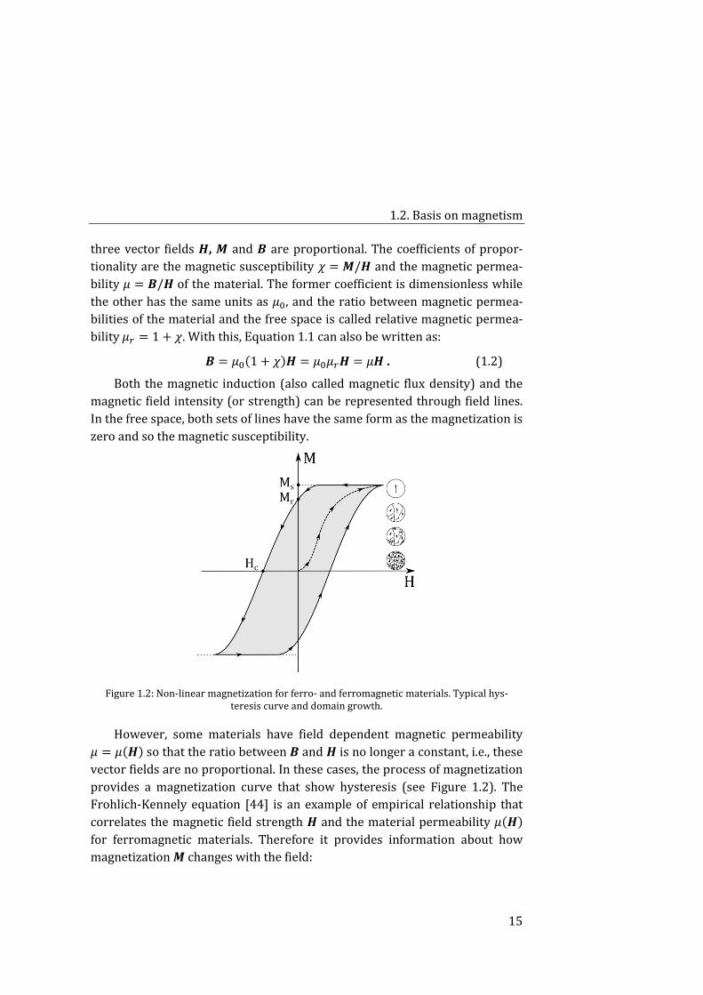
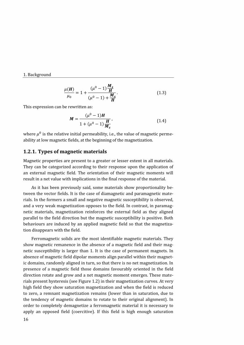
Figure 1.2: Non-linear magnetization for ferro- and ferromagnetic materials. Typical hys-teresis curve and domain growth.
However, some materials have field dependent magnetic permeability
𝜇 = 𝜇(𝑯) so that the ratio between 𝑩 and 𝑯 is no longer a constant, i.e., these
vector fields are no proportional. In these cases, the process of magnetization
provides a magnetization curve that show hysteresis (see Figure 1.2). The
Frohlich-Kennely equation [44] is an example of empirical relationship that
correlates the magnetic field strength 𝑯 and the material permeability 𝜇(𝑯)
for ferromagnetic materials. Therefore it provides information about how
magnetization 𝑴 changes with the field:
1. Background
16
𝜇(𝑯)
𝜇0= 1 +
(𝜇0 − 1)𝑴𝒔𝑯
(𝜇0 − 1) +𝑴𝒔𝑯
. (1.3)
This expression can be rewritten as:
𝑴 =(𝜇0 − 1)𝑯
1 + (𝜇0 − 1)𝑯
𝑴𝒔
, (1.4)
where 𝜇0 is the relative initial permeability, i.e., the value of magnetic perme-
ability at low magnetic fields, at the beginning of the magnetization.
Types of magnetic materials 1.2.1.
Magnetic properties are present to a greater or lesser extent in all materials.
They can be categorized according to their response upon the application of
an external magnetic field. The orientation of their magnetic moments will
result in a net value with implications in the final response of the material.
As it has been previously said, some materials show proportionality be-
tween the vector fields. It is the case of diamagnetic and paramagnetic mate-
rials. In the formers a small and negative magnetic susceptibility is observed,
and a very weak magnetization opposes to the field. In contrast, in paramag-
netic materials, magnetization reinforces the external field as they aligned
parallel to the field direction but the magnetic susceptibility is positive. Both
behaviours are induced by an applied magnetic field so that the magnetiza-
tion disappears with the field.
Ferromagnetic solids are the most identifiable magnetic materials. They
show magnetic remanence in the absence of a magnetic field and their mag-
netic susceptibility is larger than 1. It is the case of permanent magnets. In
absence of magnetic field dipolar moments align parallel within their magnet-
ic domains, randomly aligned in turn, so that there is no net magnetization. In
presence of a magnetic field those domains favourably oriented in the field
direction rotate and grow and a net magnetic moment emerges. These mate-
rials present hysteresis (see Figure 1.2) in their magnetization curves. At very
high field they show saturation magnetization and when the field is reduced
to zero, a remnant magnetization remains (lower than in saturation, due to
the tendency of magnetic domains to rotate to their original alignment). In
order to completely demagnetize a ferromagnetic material it is necessary to
apply an opposed field (coercitive). If this field is high enough saturation
1.2. Basis on magnetism
17
again reappears. As a function of the value of the coercitive field and the area
of the hysteresis loop, ferromagnetic materials can be soft or hard. For low
values of coercivity, tipically less than 1000 A/m, the material is magnetically
soft, and for values above 10000 A/m it is considered a hard material [44].
Besides, soft magnetic materials have low anisotropy and wide domain walls
while hard magnetic materials present opposite features. Ferromagnetic sys-
tems become paramagnetic, i.e., their hysteresis loops vanish as both coercivi-
ty and remanence go to zero, above the Curie temperature of the materials as
the parallel alignment of magnetic moments becomes disordered because of
thermal energy. In magnetorheological fluids it is desirable to have particles
with small coercivity and remnant magnetization (i.e., magnetically soft mate-
rials) so that the magnetizing/demagnetizing process to be carried out at
lower field strengths (easy process), as well as large saturation magnetization
for the applied field.
Other types of magnetic materials include antiferromagnet, ferrimagnets,
and superparamagnet. They share the magnetic order with ferromagnets. In
presence of a magnetic field antiferromagnetic dipoles display antiparallel
(aligned in opposite directions) resulting in zero net moment. A particular
case of antiferromagnetism appears in ferrimagnetic materials. They have
similar macroscopic trends to ferromagnets in response to a magnetic field as
a net magnetic moment is obtained during the antiparallel alignment, due to
different magnitude of magnetic moments, but show lower electric conductiv-
ity. They also exhibit hysteresis and saturation. Ferrimagnetic materials are
called ferrites, like magnetite Fe3O4. Finally, superparamagnetism occurs in
sufficiently small (single-domain) ferromagnetic or ferrimagnetic nanoparti-
cles with no long-range order between particles. In this form of magnetism
temperature randomly affect the direction of the magnetization. This behav-
iour is found in colloidal magnetic fluids, i.e., ferrofluids.
Rheology 1.3.
Rheology is the study of the deformation and flow of matter. This term was
coined in 1928 by Eugene C. Bingham, from the Greek words ρέω and λόγοσ
(meaning flow and study, respectively). This concept was investigated by
Robert Hook and Isaac Newton, who stablished concepts and laws related to
plasticity and body deformations. The Hookean elastic solid just like the New-
tonian viscous fluid are ideal substances that constitute the true limits of the
1. Background
18
rheological behaviour. However, most materials exhibit both elastic and vis-
cous features, they are viscoelastic.
Types of materials and their rheological response 1.3.1.
Hooke’s law (1678) of elasticity is a constitutive equation describing the be-
haviour of a perfect elastic solid. This empirical law states that in an elastic
body the deformation is proportional to the applied force (or stress) that
produces this deformation:
𝜎 = 𝐺𝛾 , (1.5)
where 𝜎 is the stress, 𝐺 is the elastic modulus and 𝛾 the strain. The rheologi-
cal behaviour is independent of time and there is no lag between the applica-
tion of the load and the deformation. It implies that deformation completely
disappears when the load is retired and the body recovers its initial shape.
Although it is referred to a theoretical solid, in practice, many substances can
be considered as ideally elastic.
Newton’s law, for its part, is the constitutive law applying to viscous flu-
ids. The dynamic viscosity 휂 is defined as the ratio between the tangential
tension 𝜏 = 𝐹/𝐴 (shear stress, i.e., the shear force per surface area) and the
velocity gradient �̇� = 𝜈/ℎ (shear rate), which is in turn the ratio between fluid
velocity and the height of the volume element, so that
𝜏 = 휂 �̇� . (1.6)
A fluid obeying this linear relation is called Newtonian, it is, 휂 is inde-
pendent of �̇�. Newtonian behaviour is then characterized by a constant vis-
cosity, which is also independent of the time of shearing and a permanent de-
formation. Analogously to the elastic solid, the Newtonian liquid is irreal but
many liquids are considered to be Newtonian in a broad range of shear
stresses. Water, honey and silicone oils are typical examples of Newtonian
liquids.
With this, most fluids exhibit non-Newtonian behaviours, i.e., the rela-
tionship between shear stress and shear rate is not linear. Thus viscosity may
depend on shear rate, time or present partial recovery. Non-linear fluids can
be classified as time-independent, time-dependent and viscoelastic fluids. In
Figure 1.3 the rheological behaviour of different types of fluids subjected to
shear flow are schematically shown.
1.3. Rheology
19
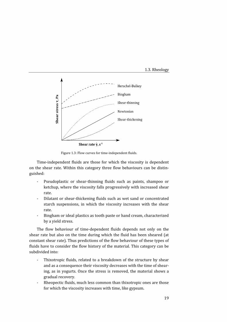
Figure 1.3: Flow curves for time-independent fluids.
Time-independent fluids are those for which the viscosity is dependent
on the shear rate. Within this category three flow behaviours can be distin-
guished:
- Pseudoplastic or shear-thinning fluids such as paints, shampoo or
ketchup, where the viscosity falls progressively with increased shear
rate.
- Dilatant or shear-thickening fluids such as wet sand or concentrated
starch suspensions, in which the viscosity increases with the shear
rate.
- Bingham or ideal plastics as tooth paste or hand cream, characterized
by a yield stress.
The flow behaviour of time-dependent fluids depends not only on the
shear rate but also on the time during which the fluid has been sheared (at
constant shear rate). Thus predictions of the flow behaviour of these types of
fluids have to consider the flow history of the material. This category can be
subdivided into:
- Thixotropic fluids, related to a breakdown of the structure by shear
and as a consequence their viscosity decreases with the time of shear-
ing, as in yogurts. Once the stress is removed, the material shows a
gradual recovery.
- Rheopectic fluids, much less common than thixotropic ones are those
for which the viscosity increases with time, like gypsum.
1. Background
20
Most materials are viscoelastic, it is, they show both fluid-like or solid-
like properties on different timescales, so that the solid and fluid parts are not
pure elastic nor pure viscous, respectively. Moreover they exhibit partial re-
covery after deformation. Viscoelasticity is then related to the materials’ abil-
ity to store (elastic) or dissipate (visco) energy. One well-known example of
viscoelastic material is the classic Silly Putty, whose main ingredient is poly-
dimethylsiloxane (a silicone-based polymer) mixed with boric acid. This
paste, which has no practical application other than as a toy, was discovered
in 1943 by the engineer James Wright while searching for inexpensive substi-
tutes for synthetic rubber. At rest it spread like a viscous liquid because the
material has time to adapt to the change in the applied stresses or defor-
mations, compared to the time scale of the process, but it bounces when
throw against the soil.
The response of the viscoelastic materials to an applied load is then a
matter of characteristic time scales, as Reiner pointed out. The well-known
Déborah number [45] was defined to quantify the ratio between the relaxa-
tion time of the material 𝑡𝑟 and the observation time 𝑡𝑜(for linear viscoelastic-
ity):
𝐷𝑒 = 𝑡𝑟/𝑡𝑜 . (1.7)
This number highlights the relative importance of elastic phenomena. In
this sense, for values of this dimensionless number well below the unity the
system behaves like more viscous, whereas it show elastic solid-like features
at higher Deborah numbers and the material behaviour changes to a non-
Newtonian regime.
Constitutive equations and material functions 1.3.2.
Constitutive equations are relationships that describe the response of a mate-
rial to stress or to deformation. Mass and momentum balance equations [46]
enables us, together with the constitutive equation, to solve flow problems.
Continuity equation:
0 =𝜕𝜌
𝜕𝑡+ ∇ · (𝜌�̅�) . (1.8)
Equation of motion:
𝜌𝐷�̅�
𝐷𝑡= 𝜌 (
𝜕�̅�
𝜕𝑡+ �̅� · ∇�̅�) = −∇ · Π̿ + 𝜌�̅� . (1.9)
1.3. Rheology
21
The total stress tensor Π̿ = p I̿ + τ̿ has two main contributions: the ther-
modynamic pressure, which is isotropic, and the contribution depending on
the flow field, originated from the fluid deformation. The equation that ex-
presses the so-called extra stress tensor τ̿ as a function of the flow field is the
stress constitutive equation. This equation must be valid for any kind of flow.
Once this expression is known, the total stress tensor is inserted in the equa-
tion of motion and, considering the continuity equation and the boundary
conditions of the systems, the solution of the velocity field can be obtained.
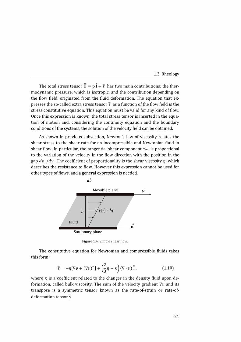
As shown in previous subsection, Newton’s law of viscosity relates the
shear stress to the shear rate for an incompressible and Newtonian fluid in
shear flow. In particular, the tangential shear component τ21 is proportional
to the variation of the velocity in the flow direction with the position in the
gap 𝑑𝑣𝑥/𝑑𝑦 . The coefficient of proportionality is the shear viscosity 휂, which
describes the resistance to flow. However this expression cannot be used for
other types of flows, and a general expression is needed.
Figure 1.4: Simple shear flow.
The constitutive equation for Newtonian and compressible fluids takes
this form:
τ̿ = −휂[∇�̅� + (∇�̅�)𝑇] + (2
3휂 − 𝜅) (∇ · �̅�) I ̿, (1.10)
where 𝜅 is a coefficient related to the changes in the density fluid upon de-
formation, called bulk viscosity. The sum of the velocity gradient ∇�̅� and its
transpose is a symmetric tensor known as the rate-of-strain or rate-of-
deformation tensor γ̿̇.
1. Background
22
In the case of incompressible (i.e., fluid density is constant) Newtonian
fluids, the constitutive equation simplifies as
τ̿ = −휂 γ̿̇ , (1.11)
and substituting Equation 1.11 into the equation of motion the well-known
Navier-Stokes equation for incompressible Newtonian fluid results:
𝜌𝐷�̅�
𝐷𝑡= −∇𝑝 + 휂∇2�̅� + 𝜌�̅� . (1.12)
However, the description of the flow of non-Newtonian fluids, i.e., its
changes with position and time, is more complex. Equation 1.11 and 1.12 do
not apply for these materials and other non-linear constitutive equations
have to be developed to model their behaviour. A constitutive equation that
predict some experimentally observed non-Newtonian behaviours is the gen-
eralized Newtonian fluid (GNF) model [47]. It stands out for being a first and
simple approach that matches steady shearing data very well (although it is
unclear its validity in non-shear flows) and that is useful for predicting pres-
sure-drop relationships and flow-rate information. This stress-deformation
law is alike to that for incompressible Newtonian fluids, but instead the fluid
viscosity is taken as a shear rate dependent viscosity:
τ̿ = −휂(γ̇)γ̿̇ , (1.13)
where γ̇ = |γ̿̇|.
This expression comply the physical and mathematical constrains that
guarantee the mathematical sense of the tensorial equation. The viscosity de-
pendence 휂(γ̇) can take multiple forms [47,48]. Among them, we can high-
light power-law models, Carreau-Yasuda or Cross model, and yield stress
models. Their expressions are shown in Table 1.1.
The power-law (or Ostwald-de Waele) model provides an empirical and
simple relationship between viscosity and shear rate with two parameters
that can fit reasonably well for shear thinning or shear thickening fluids in
limited ranges of shear rates.
The Carreau-Yasuda model accounts better the shape of viscosity curves
as it considers five parameters. Specifically, constant viscosity values (plat-
eaus) at zero 휂0 and infinite shear rate 휂∞ are predicted, a critical shear rate
�̇�𝑐 determines the transition from one value to another, and the curvature and
slope of the transition is modelled with 𝑎 and 𝑛, respectively.
1.3. Rheology
23
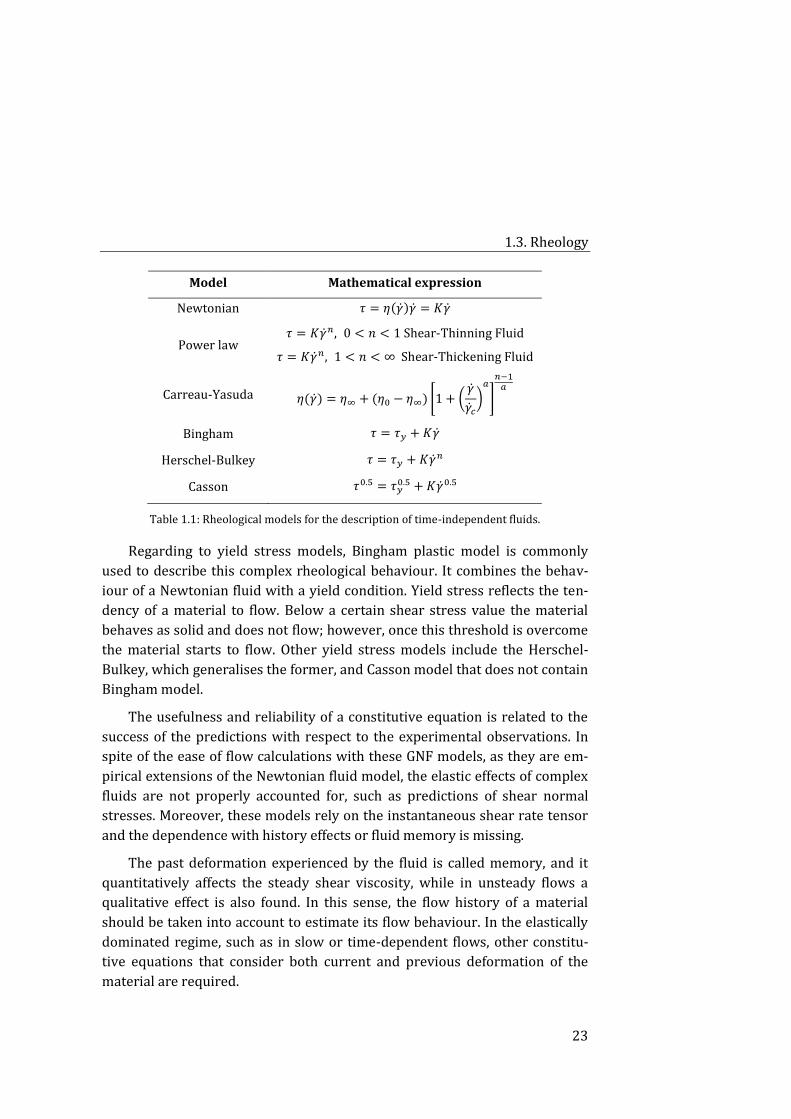
Model Mathematical expression
Newtonian 𝜏 = 휂(�̇�)�̇� = 𝐾�̇�
Power law 𝜏 = 𝐾�̇�𝑛, 0 < 𝑛 < 1 Shear-Thinning Fluid
𝜏 = 𝐾�̇�𝑛, 1 < 𝑛 < ∞ Shear-Thickening Fluid
Carreau-Yasuda 휂(�̇�) = 휂∞ + (휂0 − 휂∞) [1 + (�̇�
�̇�𝑐
)𝑎
]
𝑛−1𝑎
Bingham 𝜏 = 𝜏𝑦 + 𝐾�̇�
Herschel-Bulkey 𝜏 = 𝜏𝑦 + 𝐾�̇�𝑛
Casson 𝜏0.5 = 𝜏𝑦0.5 + 𝐾�̇�0.5
Table 1.1: Rheological models for the description of time-independent fluids.
Regarding to yield stress models, Bingham plastic model is commonly
used to describe this complex rheological behaviour. It combines the behav-
iour of a Newtonian fluid with a yield condition. Yield stress reflects the ten-
dency of a material to flow. Below a certain shear stress value the material
behaves as solid and does not flow; however, once this threshold is overcome
the material starts to flow. Other yield stress models include the Herschel-
Bulkey, which generalises the former, and Casson model that does not contain
Bingham model.
The usefulness and reliability of a constitutive equation is related to the
success of the predictions with respect to the experimental observations. In
spite of the ease of flow calculations with these GNF models, as they are em-
pirical extensions of the Newtonian fluid model, the elastic effects of complex
fluids are not properly accounted for, such as predictions of shear normal
stresses. Moreover, these models rely on the instantaneous shear rate tensor
and the dependence with history effects or fluid memory is missing.
The past deformation experienced by the fluid is called memory, and it
quantitatively affects the steady shear viscosity, while in unsteady flows a
qualitative effect is also found. In this sense, the flow history of a material
should be taken into account to estimate its flow behaviour. In the elastically
dominated regime, such as in slow or time-dependent flows, other constitu-
tive equations that consider both current and previous deformation of the
material are required.
1. Background
24
An example of constitutive equation for shear flows that incorporates
some elastic effects was proposed by James Clerk Maxwell in 1867. In its sca-
lar form Maxwell equation is given by:
𝜏21 +휂
𝐺
𝜕𝜏21
𝜕𝑡 = −휂�̇�21 , (1.14)
which converts into Newton’s law when temporal effects are insignificant and
into Hook’s law for rapid motions at short times, as the derivative term great-
ly exceed the stress.
In steady simple shear flow (see Figure 1.4), the flow is generated as a
consequence of the relative motion of one flat plate relative to another. These
plates are parallel and the gap between them is constant. Due to the sym-
metry of the stress tensor, only four components are nonzero in this type of
flow: normal stress components (i.e., diagonal elements: 𝜏11, 𝜏22, 𝜏33) and the
shear stress 𝜏21 = 𝜏12. The differences between normal components can gen-
erate deformation and they have more rheological interest than the magni-
tude of these components. This lead to the definition of two stress-related
quantities, the first and second normal stress differences, as follows:
𝑁1(�̇�) = 𝜏11 − 𝜏22; 𝑁2(�̇�) = 𝜏22 − 𝜏33 . (1.15)
In the case of Newtonian fluids, the shear stress is proportional to the
shear rate 𝜏(�̇�) = 𝜏21 = 휂�̇�, and normal stress differences are zero. The state
of stress of a fluid in viscometric flow is fully described with three shear-rate-
dependent material functions, which are related to 𝜏, 𝑁1, and 𝑁2. They are
called viscosity, first normal stress coefficient and second normal stress coef-
ficient, respectively:
휂(�̇�) =𝜏
�̇�; 𝜓1(�̇�) =
𝑁1
�̇�2; 𝜓2(�̇�) =
𝑁2
�̇�2 . (1.16)
Material functions have the same values whatever the viscometric flow
used, and can be predicted once the constitutive equations are known and the
stress responses are measured.
Effect of volume fraction in viscosity 1.3.3.
In the ideal case of hard spheres, one of the simplest cases of non-interacting
systems, the apparent viscosity 휂𝑎𝑝𝑝 in the case of dilute systems (below a
concentration of 5 %) can be calculated through the well-known Einstein
equation [49,50]. It is a linear function of the particle volume fraction
1.3. Rheology
25
𝜙 =𝑉𝑝
𝑉𝑝+𝑉𝑓, i.e., the ratio between the particle 𝑉𝑝 and total system volume
𝑉 = 𝑉𝑝 + 𝑉𝑓 (for a suspension containing 𝑁 spheres with radius 𝑎,
𝜙 =4
3𝜋𝑎3 𝑁
𝑉 ), as follows:
휂𝑟 =휂𝑎𝑝𝑝
휂𝑠= (1 + 2.5𝜙) . (1.17)
This expression is valid when there is no internal dissipation but only
that from the fluid, so that this relation is useful for emulsions as particles in
these systems are liquid. The linearity with the concentration appears as a
consequence of particles not interacting each other and so the deformation of
the flow due to each particle is additive. Moreover, as can be observed, this
expression is independent of the size, shape, polydispersity, and density of
the particles. So that for two different systems the suspension viscosity would
be the same if the carrier fluid and the particle concentration coincide.
In the semi-dilute regime (0.05<𝜙<0.15) the distance between particles is
comparable to the particle size and interactions of nearby particles provoke a
higher energy dissipation. Again, the suspension viscosity depends on the
volume fraction and viscosity of the medium. Both the effects of hydrodynam-
ic interactions in the suspension viscosity and the Brownian motion were
considered by Batchelor [51] by including a term of order 𝜙2:
휂𝑟 = 1 + 2.5𝜙 + 6.2𝜙2 . (1.18)
Polydispersity comes into play in this regime because hydrodynamic
forces are affected by the distance between particles compared to their size. A
higher polydispersity reduces the system viscosity as for a given volume frac-
tion polydispersity results in more free space to flow (better packing), but
this effect competes with the increase in viscosity caused by the increase in
particle-particle interactions when the particle size decreases.
In concentrated systems, the viscosity rapidly increases due to the fact
that multi-particle interactions become decisive, and near the maximum
packing fraction it diverges. This is a problem in theoretical methods, and alt-
hough a determining method is lacking particle level simulations can be help-
ful in the determination of the suspension viscosity if the employed time steps
are low enough.
In practice, viscosity models for more concentrated suspensions often use
semi-empirical expressions with an adjustable parameter, the maximum vol-
1. Background
26
ume fraction 𝜙𝑚, before which the viscosity would become infinite in the
equation relating the relative viscosity and the particle concentration. This
parameter depends on the shape and size distribution of suspended particles.
A great number of viscosity relations take the form of 휂𝑟 = 휂𝑟(𝜙, 𝜙𝑚). In the
case of monodisperse hard spheres the maximum packing fraction capable to
flow is 𝜙𝑟𝑐𝑝 = 0.64, that corresponds with a random close packing. Quemada
[52] included this parameter within his model as follows:
휂𝑟 = (1 −𝜙
𝜙𝑚)
−2
. (1.19)
Suspensions with higher polydispersity can better densify the packing, as
smaller particles occupy holes between big particles. As it has been previous-
ly said this provokes a decrease in viscosity for a given volume fraction. The
maximum packing depends on the size distribution and particle shape but not
on particle size.
The model developed by Irvin Krieger and Thomas Dougherty [53] con-
siders a different exponent:
휂𝑟 = (1 −𝜙
𝜙𝑚)
−𝜂1𝜙𝑚
, (1.20)
where 휂1 is an intrinsic viscosity dependent on the particle shape, that takes
the value of 2.5 for spheres. If the suspension show non-Newtonian behaviour
(see Subsection 1.3.1), the predictive models of the suspension viscosity
should include a shear-rate dependent term. If not included in the model, the
viscosity could be estimated only in tight regions (low or high shear rate
Newtonian regions).
Tribology 1.4.
Generalities 1.4.1.
Tribology is defined as the science that deals with the design, friction, wear,
and lubrication of interacting surfaces in relative motion. This word also de-
rives from the Greek and the literal translation would be the “science of rub-
bing”. The term tribology was coined by Hans Peter Jost, who in 1966 pub-
lished a landmark report on the costs of friction, wear and corrosion to the
UK economy, titled “Lubrication (Tribology), Education and Research: A Report
on the Present Position and Industry’s Needs” [54]. In fact, the analysis of tribo-
1.4. Tribology
27
logical behaviour in technical equipment tackles remarkable economic prob-
lems, ranging from spacecraft to household applications. In this sense, the
successful in machine elements design (and durability), and the minimization
of losses (i.e., energy efficiency) from friction and wear greatly depends on
the understanding of tribological principles. However, tribology not only af-
fects industrial applications but also our daily life, like in the process of writ-
ing (pencil/paper contact), walking (shoes/ground contact) or in many joints
in the human body.
The relative motion between two surfaces entails the appearance of dis-
sipative phenomena that produces heat and resists to this movement, i.e., fric-
tion. Indeed, the origin of friction comes from the deformation of the contact-
ing surface roughness or asperities, as a consequence of the relative move-
ment and the load. Two types of friction are distinguished: static friction oc-
curring between quiet surfaces in contact and dynamic friction which
concerns the resistance to relative motion between the surfaces after the
movement starts. This distinction was made by Coulomb, and each type of
friction can be quantified with dimensionless parameters called static 𝜇 and
dynamic 𝑘 friction coefficients. They are given by the ratio of the frictional
force 𝐹 to the applied load 𝑊.
Observations of the physicist Guillaume Amontons (1699) and years later
by Charles-Augustin Coulomb (1785) resulted in three laws governing fric-
tion:
- First law (Amontons): the friction force is directly proportional to the
normal load, so that 𝐹 = 𝜇𝑊.
- Second law (Amontons): the friction force is independent of the ap-
parent area of contact.
- Third law (Coulomb): the dynamic friction is independent of velocity
once motion starts.
Wear is the progressive removal of material from a surface in relative
motion with other surface or with a fluid. It plays a fundamental role in tri-
bology as it causes damage or changes in the shape of the components. These
changes are comparable to elastic deformation and have to be considered in
the distribution of stresses or in the dimensions of contacting areas. However,
wear is not always seen as an unwanted consequence of friction since it is of-
ten used to reduce the roughness or eliminate asperities in some materials.
There are distinct types of wear such as adhesive, abrasive, fatigue, or corro-
1. Background
28
sive wear. Contrarily to what could be thought a larger friction may not entail
a larger wear. The true is that the relationship between these phenomena is
not necessarily proportional but rather the frictional energy distribution var-
ies in different tribosystems.
In order to control friction and wear a proper lubrication between the
components is required and with this purpose some materials, coatings or
surface treatments are used. In this sense, lubricants are materials (liquids,
solids or gases) characterized by their viscosity that contributes to reduce
friction between surfaces, as they avoid the direct contact between surfaces
and thus restrict the wear.
The lubrication behaviour is measured with a tribometer and can be un-
derstood with the Stribeck curve. It is a plot that relates the coefficient of fric-
tion and a parameter that combines the fluid viscosity, the relative speed of
surface movement and the applied load. The unit of this combined parameter
has unit of a length and is somehow seen as the lubricant film thickness be-
tween the surfaces in movement. Stribeck curve tipically contains three lubri-
cation regimes as can be observed in Figure 1.5. The lubrication conditions
are affected by the applied load, speed, and properties of the fluid lubricant
and the contacting surfaces:
- At small relative motion between surfaces the lubricant hardly enters
the contact, so that the separation is small, the surface asperities are
in direct contact and they are the main responsible for supporting the
applied load. This is called boundary lubrication regime and reflects a
scenario where the friction force is highly related to the surface
roughness. This region is characterized by a high value of the friction
coefficient, which is governed by the physicochemical properties of
both the fluid film and surfaces.
- A higher lubricant entrainment is induced at moderate speeds, where
the surface separation increases. This produces a decreasing trend in
friction coefficient with increasing the speed in the Stribeck curve.
This regime, known as mixed lubrication regime, is driven by the bulk
properties of the lubricant and the surface topography, where only
large asperities contribute to friction.
- The last part in the Stribeck curve is the hydrodynamic lubrication or
full-film regime. Higher entrainment speeds permit the lubricant ful-
ly enters the contact and this thick film completely separates the solid
surfaces. In this regime, the load is fully supported by the lubricant so
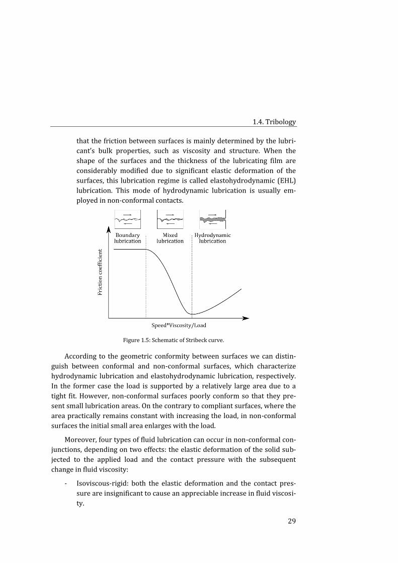
1.4. Tribology
29
that the friction between surfaces is mainly determined by the lubri-
cant’s bulk properties, such as viscosity and structure. When the
shape of the surfaces and the thickness of the lubricating film are
considerably modified due to significant elastic deformation of the
surfaces, this lubrication regime is called elastohydrodynamic (EHL)
lubrication. This mode of hydrodynamic lubrication is usually em-
ployed in non-conformal contacts.
Figure 1.5: Schematic of Stribeck curve.
According to the geometric conformity between surfaces we can distin-
guish between conformal and non-conformal surfaces, which characterize
hydrodynamic lubrication and elastohydrodynamic lubrication, respectively.
In the former case the load is supported by a relatively large area due to a
tight fit. However, non-conformal surfaces poorly conform so that they pre-
sent small lubrication areas. On the contrary to compliant surfaces, where the
area practically remains constant with increasing the load, in non-conformal
surfaces the initial small area enlarges with the load.
Moreover, four types of fluid lubrication can occur in non-conformal con-
junctions, depending on two effects: the elastic deformation of the solid sub-
jected to the applied load and the contact pressure with the subsequent
change in fluid viscosity:
- Isoviscous-rigid: both the elastic deformation and the contact pres-
sure are insignificant to cause an appreciable increase in fluid viscosi-
ty.
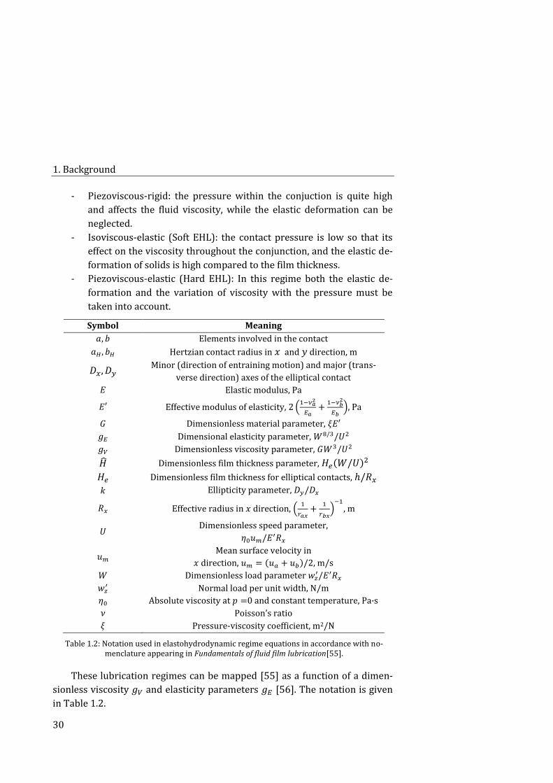
1. Background
30
- Piezoviscous-rigid: the pressure within the conjuction is quite high
and affects the fluid viscosity, while the elastic deformation can be
neglected.
- Isoviscous-elastic (Soft EHL): the contact pressure is low so that its
effect on the viscosity throughout the conjunction, and the elastic de-
formation of solids is high compared to the film thickness.
- Piezoviscous-elastic (Hard EHL): In this regime both the elastic de-
formation and the variation of viscosity with the pressure must be
taken into account.
Symbol Meaning
𝑎, 𝑏 Elements involved in the contact
𝑎𝐻 , 𝑏𝐻 Hertzian contact radius in 𝑥 and 𝑦 direction, m
𝐷𝑥, 𝐷𝑦 Minor (direction of entraining motion) and major (trans-
verse direction) axes of the elliptical contact
𝐸 Elastic modulus, Pa
𝐸′ Effective modulus of elasticity, 2 (1−𝜈𝑎
2
𝐸𝑎+
1−𝜈𝑏2
𝐸𝑏), Pa
𝐺 Dimensionless material parameter, 𝜉𝐸′
𝑔𝐸 Dimensional elasticity parameter, 𝑊8/3/𝑈2
𝑔𝑉 Dimensionless viscosity parameter, 𝐺𝑊3/𝑈2
�̂� Dimensionless film thickness parameter, 𝐻𝑒(𝑊/𝑈)2
𝐻𝑒 Dimensionless film thickness for elliptical contacts, ℎ/𝑅𝑥
𝑘 Ellipticity parameter, 𝐷𝑦/𝐷𝑥
𝑅𝑥 Effective radius in 𝑥 direction, (1
𝑟𝑎𝑥+
1
𝑟𝑏𝑥)
−1
, m
𝑈 Dimensionless speed parameter,
휂0𝑢𝑚/𝐸′𝑅𝑥
𝑢𝑚 Mean surface velocity in
𝑥 direction, 𝑢𝑚 = (𝑢𝑎 + 𝑢𝑏)/2, m/s
𝑊 Dimensionless load parameter 𝑤𝑧′/𝐸′𝑅𝑥
𝑤𝑧′ Normal load per unit width, N/m
휂0 Absolute viscosity at 𝑝 =0 and constant temperature, Pa·s
𝜈 Poisson’s ratio
𝜉 Pressure-viscosity coefficient, m2/N
Table 1.2: Notation used in elastohydrodynamic regime equations in accordance with no-menclature appearing in Fundamentals of fluid film lubrication[55].
These lubrication regimes can be mapped [55] as a function of a dimen-
sionless viscosity 𝑔𝑉 and elasticity parameters 𝑔𝐸 [56]. The notation is given
in Table 1.2.
1.4. Tribology
31
In compliant contacts both rolling and sliding frictions have to be taken
into account, while in non-conformal ones, rolling friction can be neglected in
comparison with sliding friction. The ratio between sliding speed (the relative
velocity difference between the contacting surfaces) and entraining speeds
(the mean of rolling speeds of two surfaces relative to the contact) is ex-
pressed by the slide-to-roll ratio 𝑆, which will be further developed. In this
sense, in pure rolling conditions 𝑆 = 0.
When two elastic bodies approach, a contact area appears whose form
depends on the type of surfaces and the applied load involved in the contact.
Among them, point (sphere-sphere) and line contacts (cylinder-plane) are the
most commonly encountered. However, elliptical contacts [57] cover a wider
range of deformations occurring in practice, according to the radius ratio,
from the circular point contact to near line contact
Reynolds equation 1.4.2.
In fluid film lubrication problems the predominant terms of Navier-Stokes
equations belong to pressure and viscous terms so that they are indeed slow
viscous motion problems. The pressure distribution in fluid film lubrication,
assumed to behave as a Newtonian fluid, was determined by a differential
equation derived from the Navier-Stokes equations by Osborne Reynolds in
1886 [58]. In its general form it becomes:
𝜕
𝜕𝑥(
𝜌ℎ3
12휂
𝜕𝑝
𝜕𝑥) +
𝜕
𝜕𝑦(
𝜌ℎ3
12휂
𝜕𝑝
𝜕𝑦) =
=𝑢𝑎 + 𝑢𝑏
2
𝜕
𝜕𝑥(𝜌ℎ) +
𝑣𝑎 + 𝑣𝑏
2
𝜕
𝜕𝑦(𝜌ℎ) +
+𝜌(𝑤𝑎 − 𝑤𝑏) − 𝜌𝑢𝑎
𝜕ℎ
𝜕𝑥− 𝜌𝑣𝑎
𝜕ℎ
𝜕𝑦+
𝜕
𝜕𝑡(𝜌ℎ) ,
(1.21)
where 𝑝, ℎ, 𝜌, and 휂 are the pressure, film thickness, density and viscosity of
the lubricant, and 𝑢𝑖, 𝑣𝑖, and 𝑤𝑖 denote the components of the velocity surfac-
es of an 𝑖-body in 𝑥, 𝑦 and 𝑧 directions, respectively.
The Reynolds equation cover four terms, whose physical meaning [55]
are exposed below:
- Poiseuille terms, in the left side of the equation, describe the net flow
rates due to pressure gradients within the lubricated area.
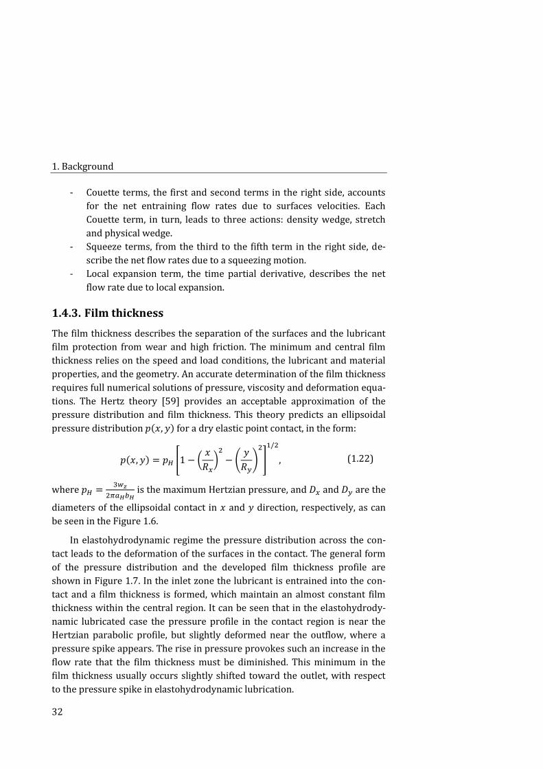
1. Background
32
- Couette terms, the first and second terms in the right side, accounts
for the net entraining flow rates due to surfaces velocities. Each
Couette term, in turn, leads to three actions: density wedge, stretch
and physical wedge.
- Squeeze terms, from the third to the fifth term in the right side, de-
scribe the net flow rates due to a squeezing motion.
- Local expansion term, the time partial derivative, describes the net
flow rate due to local expansion.
Film thickness 1.4.3.
The film thickness describes the separation of the surfaces and the lubricant
film protection from wear and high friction. The minimum and central film
thickness relies on the speed and load conditions, the lubricant and material
properties, and the geometry. An accurate determination of the film thickness
requires full numerical solutions of pressure, viscosity and deformation equa-
tions. The Hertz theory [59] provides an acceptable approximation of the
pressure distribution and film thickness. This theory predicts an ellipsoidal
pressure distribution 𝑝(𝑥, 𝑦) for a dry elastic point contact, in the form:
𝑝(𝑥, 𝑦) = 𝑝𝐻 [1 − (𝑥
𝑅𝑥)
2
− (𝑦
𝑅𝑦)
2
]
1/2
, (1.22)
where 𝑝𝐻 =3𝑤𝑧
2𝜋𝑎𝐻𝑏𝐻 is the maximum Hertzian pressure, and 𝐷𝑥 and 𝐷𝑦 are the
diameters of the ellipsoidal contact in 𝑥 and 𝑦 direction, respectively, as can
be seen in the Figure 1.6.
In elastohydrodynamic regime the pressure distribution across the con-
tact leads to the deformation of the surfaces in the contact. The general form
of the pressure distribution and the developed film thickness profile are
shown in Figure 1.7. In the inlet zone the lubricant is entrained into the con-
tact and a film thickness is formed, which maintain an almost constant film
thickness within the central region. It can be seen that in the elastohydrody-
namic lubricated case the pressure profile in the contact region is near the
Hertzian parabolic profile, but slightly deformed near the outflow, where a
pressure spike appears. The rise in pressure provokes such an increase in the
flow rate that the film thickness must be diminished. This minimum in the
film thickness usually occurs slightly shifted toward the outlet, with respect
to the pressure spike in elastohydrodynamic lubrication.
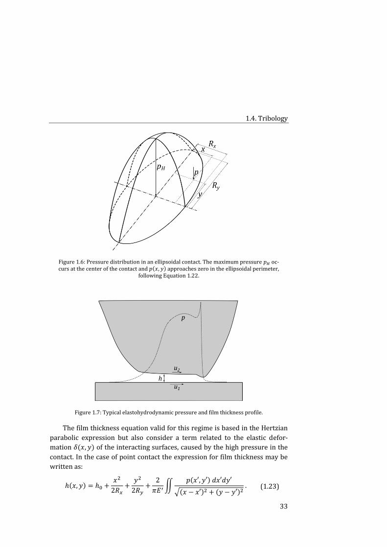
1.4. Tribology
33
Figure 1.6: Pressure distribution in an ellipsoidal contact. The maximum pressure 𝑝𝐻 oc-curs at the center of the contact and 𝑝(𝑥, 𝑦) approaches zero in the ellipsoidal perimeter,
following Equation 1.22.
Figure 1.7: Typical elastohydrodynamic pressure and film thickness profile.
The film thickness equation valid for this regime is based in the Hertzian
parabolic expression but also consider a term related to the elastic defor-
mation 𝛿(𝑥, 𝑦) of the interacting surfaces, caused by the high pressure in the
contact. In the case of point contact the expression for film thickness may be
written as:
ℎ(𝑥, 𝑦) = ℎ0 +𝑥2
2𝑅𝑥+
𝑦2
2𝑅𝑦+
2
𝜋𝐸′∬
𝑝(𝑥′, 𝑦′) 𝑑𝑥′𝑑𝑦′
√(𝑥 − 𝑥′)2 + (𝑦 − 𝑦′)2 . (1.23)
1. Background
34
A general expression for the dimensionless film thickness parameter �̂�
appears below. The dimensionless central and minimum film thicknesses
vary for different film lubrication regions, and this set of film thickness equa-
tions are based on two dimensionless parameter, 𝑈 and 𝑊:
�̂� = 𝐻𝑒 (𝑊
𝑈)
2
. (1.24)
The applied load must be balanced with the pressure generated in the flu-
id film. In this sense, the integral of the pressure distribution over the contact
area must fit the value of the load:
𝑤𝑧 = ∬ 𝑝(𝑥, 𝑦)𝑑𝑥𝑑𝑦 . (1.25)
Although most lubricants are Newtonian others may present Non-
Newtonian behaviour. They exhibit a nonlinear relationship between shear
stress and shear rate, so that the expression of viscosity that has to be insert-
ed in Reynolds equation becomes more complex. For example, the shear-
thinning behaviour of polymer melts is accurately predicted with the Car-
reau-Yasuda model, where the fit at both low and high shear rates is better
than with the power-law model. Carreau-Yasuda model predicts two Newto-
nian plateaus at low and high shear rates, and the transition between these
states can be adjusted through variations in its parameters. In this sense this
model would not be only restricted to shear thinning fluids, and could be ap-
plicable to shear-thickening fluids if the Newtonian plateau at low shear rates
is lower than that at high shear rates, as it will be shown in Chapters 6 and 7.
Thus, in the elastohydrodynamic regime the change in the lubrication
viscosity of a non-Newtonian fluid comes from its nonlinear behaviour but
also from the effect of the high hydrodynamic pressure in non-conformal con-
tacts, which also influences the elastic deformation of surfaces.
In this thesis predictions of the pressure distribution, film thickness and
friction coefficient for non-Newtonian fluids are tackled with numerical
modelling methods. The governing equations are first written in their nondi-
mensional forms, and secondly discretized at each pressure point. The nu-
merical solution for pressure and film thickness is then obtained after select-
ing an appropriate numerical method.
1.5. Simulation methods for colloidal suspensions
35
Simulation methods for colloidal suspensions 1.5.
Numerical simulation is a powerful tool that allows for the modelling of pro-
cesses in very distinct scientific areas. The development in computers’ effi-
ciency and computational methods offer the chance of replicating experi-
ments and explore other scenarios by easily tuning the system features, thus
saving time and money. The computational costs (in terms of simulation
time) rely on the required level of detail and accuracy in the results. In this
sense, approaches usually provide acceptable results that complement theory
and experimental observations, even if some interaction in the system has
been simplified or directly neglected. Although simulations are limited by
computational requirements they enable the prediction of macroscopic in-
formation of the system such as the effective viscosity or the temporal evolu-
tion in the microstructure.
Of particular interest in this thesis is the motion of particles suspended in
a fluid, their effect on the flow field and the resultant macroscopic behaviour.
Suspension dynamics can be properly addressed with molecular simulations,
which can be divided into four main categories [60]: Monte Carlo [61], Molec-
ular Dynamics [62], Stokesian Dynamics [63] and Brownian Dynamics meth-
ods [64,65]. Monte Carlo simulations analyse the energy of microscopic states
(particle configurations) randomly generated with a frequency proportional
to the equilibrium probability distribution. This is a non-deterministic meth-
od that is used to simulate physical phenomena for systems in thermodynam-
ic equilibrium. Molecular dynamics methods provide the temporal evolution
of the particle position and velocity by solving Newton’s motion equations.
They are deterministic and applicable to dilute systems as hydrodynamic in-
teractions among particles are neglected and so Brownian motion. Stokesian
dynamics by its part tackle the suspension dynamics in non-dilute systems,
where multi-body hydrodynamic interactions are relevant, while Brownian
motion is not taken into account. Finally, Brownian dynamics methods con-
sider Brownian motion through a random and stochastic force. Molecules of
the carrier fluid are generally much smaller than Brownian particles in dis-
persions, so that these particles are regarded as a continuum in Brownian dy-
namics. They are based on the Langevin equation for the motion of particles
in dilute dispersions, while other more complex Brownian dynamic methods
are employed when hydrodynamic interactions between particles are taken
into account (case of non-dilute systems).
1. Background
36
In Section 3.3 a detailed description of simulations employed throughout
this thesis is addressed. The rheological behaviour of suspensions of mixtures
of particles as well as squeeze simulations under constant-volume and con-
stant-area conditions will be studied through particle-level simulations. On
the other hand, the solution of the fluid film lubrication of non-Newtonian
fluids in elastohydrodynamic lubrication regime is tackled numerically.
References 1.6.
[1] Vitelli V and Hecke M van 2011 Marginal matters Nature 480 325–326
[2] Hołyst R 2005 Some features of soft matter systems Soft Matter 1 329
[3] van der Gucht J 2018 Grand challenges in soft matter physics Front. Phys. 6
[4] Nagel S R 2017 Experimental soft-matter science Rev. Mod. Phys. 89
[5] Gennes P-G de and Badoz J 1997 Fragile objects: soft matter, hard sci-ence, and the thrill of discovery Choice Rev. Online 34 34–3369–34–3369
[6] Babick F 2016 Suspensions of colloidal particles and aggregates (Springer International Publishing)
[7] Bajpai P 2018 Colloid and surface chemistry Biermann’s Handbook of Pulp and Paper (Elsevier) pp 381–400
[8] Derjaguin B V and Landau L 1941 Theory of the stability of strongly charged lyophobic sols and of the adhesion of strongly charged particles in solutions of electrolytes Acta Physicochim. URSS 14 633–622
[9] Verwey E J W and Overbeek J T G 1948 Theory of the stability of lyo-phobic colloids (Amsterdam: Elsevier)
[10] Derjaguin B V, Churaev N V and Muller V M 1987 The Derjaguin—Landau—Verwey—Overbeek (DLVO) Theory of Stability of Lyophobic Col-loids Surface Forces (Boston, MA: Springer US) pp 293–310
[11] Israelachvili J N 2011 Intermolecular and surface forces (San Diego: Academic Press)
[12] Rankin P J, Ginder J M and Klingenberg D J 1998 Electro- and magne-to-rheology Curr. Opin. Colloid Interface Sci. 3 373–381
[13] Rabinow J 1948 The magnetic fluid clutch Trans. Am. Inst. Electr. Eng. 67 1308–1315
1.6. References
37
[14] Winslow W M 1949 Induced fibration of suspensions J. Appl. Phys. 20 1137–40
[15] Ginder J 2003 Rheology controlled by magnetic fields Digit. Encycl. Appl. Phys.
[16] Odenbach S 2002 Ferrofluids vol 594 (Berlin, Heidelberg: Springer Berlin Heidelberg)
[17] Bossis G, Volkova O, Lacis S and Meunier A 2002 Magnetorheology: fluids, structures and rheology Ferrofluids (Springer Berlin Heidelberg) pp 202–230
[18] Park B J, Fang F F and Choi H J 2010 Magnetorheology: materials and application Soft Matter 6 5246
[19] Ramos J, Klingenberg D J, Hidalgo-Álvarez R and Vicente J de 2011 Steady shear magnetorheology of inverse ferrofluids J. Rheol. 55 127–152
[20] Ramos J, Vicente J de and Hidalgo-Álvarez R 2010 Small-amplitude os-cillatory shear magnetorheology of inverse ferrofluids Langmuir 26 9334–9341
[21] Salomon Stephen Papell 1965 Low viscosity magnetic fluid obtained by the colloidal suspension of magnetic particles
[22] Rosensweig R E 1997 Ferrohydrodynamics (Mineola, N.Y: Dover Publi-cations)
[23] Klingenberg D J 2001 Magnetorheology: Applications and challenges AIChE J. 47 246–249
[24] Boyer F, Guazzelli É and Pouliquen O 2011 Unifying suspension and granular rheology Phys. Rev. Lett. 107
[25] Barnes H A 1989 Shear-thickening (“Dilatancy”) in suspensions of nonaggregating solid particles dispersed in Newtonian liquids J. Rheol. 33 329–366
[26] Brown E, Forman N A, Orellana C S, Zhang H, Maynor B W, Betts D E, DeSimone J M and Jaeger H M 2010 Generality of shear thickening in dense suspensions Nat. Mater. 9 220–224
[27] Brown E and Jaeger H M 2014 Shear thickening in concentrated sus-pensions: phenomenology, mechanisms and relations to jamming Rep. Prog. Phys. 77 046602
[28] Galindo-Rosales F J, Rubio-Hernández F J and Sevilla A 2011 An ap-parent viscosity function for shear thickening fluids J. Non-Newton. Fluid Mech. 166 321–325
1. Background
38
[29] Seto R, Mari R, Morris J F and Denn M M 2013 Discontinuous shear thickening of frictional hard-sphere suspensions Phys. Rev. Lett. 111
[30] Gurnon A K and Wagner N J 2015 Microstructure and rheology rela-tionships for shear thickening colloidal dispersions J. Fluid Mech. 769 242–276
[31] Gopalakrishnan V and Zukoski C F 2004 Effect of attractions on shear thickening in dense suspensions J. Rheol. 48 1321–1344
[32] Lee Y S, Wetzel E D and Wagner N J 2003 The ballistic impact charac-teristics of Kevlar® woven fabrics impregnated with a colloidal shear thick-ening fluid J. Mater. Sci. 38 2825–2833
[33] Dawson M A, McKinley G H and Gibson L J 2009 The dynamic com-pressive response of an open-cell foam impregnated with a non-Newtonian fluid J. Appl. Mech. 76 061011
[34] Tan Z H, Zuo L, Li W H, Liu L S and Zhai P C 2016 Dynamic response of symmetrical and asymmetrical sandwich plates with shear thickening fluid core subjected to penetration loading Mater. Des. 94 105–10
[35] Metzner A B and Whitlock M 1958 Flow behavior of concentrated (di-latant) suspensions Trans. Soc. Rheol. 2 239–254
[36] Hoffman R L 1974 Discontinuous and dilatant viscosity behavior in concentrated suspensions. II. Theory and experimental tests J. Colloid Inter-face Sci. 46 491–506
[37] Hoffman R L 1982 Discontinuous and dilatant viscosity behavior in concentrated suspensions III. Necessary conditions for their occurrence in viscometric flows Adv. Colloid Interface Sci. 17 161–184
[38] Brady J F and Bossis G 1985 The rheology of concentrated suspen-sions of spheres in simple shear flow by numerical simulation J. Fluid Mech. 155 105
[39] Fernandez N, Mani R, Rinaldi D, Kadau D, Mosquet M, Lombois-Burger H, Cayer-Barrioz J, Herrmann H J, Spencer N D and Isa L 2013 Microscopic mechanism for shear thickening of non-Brownian suspensions Phys. Rev. Lett. 111
[40] Merkt F S, Deegan R D, Goldman D I, Rericha E C and Swinney H L 2004 Persistent holes in a fluid Phys. Rev. Lett. 92
[41] Waitukaitis S R and Jaeger H M 2012 Impact-activated solidification of dense suspensions via dynamic jamming fronts Nature 487 205–209
1.6. References
39
[42] Fall A, Bertrand F, Hautemayou D, Mezière C, Moucheront P, Lemaître A and Ovarlez G 2015 Macroscopic discontinuous shear thickening versus lo-cal shear jamming in cornstarch Phys. Rev. Lett. 114
[43] Gálvez L O, Beer S de, Meer D van der and Pons A 2017 Dramatic effect of fluid chemistry on cornstarch suspensions: Linking particle interactions to macroscopic rheology Phys. Rev. E 95
[44 ]Jiles D 1991 Introduction to Magnetism and Magnetic Materials (Bos-ton, MA: Springer US)
[45] Reiner M 1964 The Deborah Number Phys. Today 17 62–62
[46] Bird R B, Armstrong R C and Hassager O 1987 Dynamics of polymeric liquids. Volume 1: Fluid mechanics
[47] Morrison F 2001 Understanding rheology (New York: Oxford Universi-ty Press)
[48] Steffe J F 1996 Rheological methods in food process engineering (East Lansing, MI: Freeman Press)
[49] Einstein A 1905 Über die von der molekularkinetischen. Theorie der Wärme geforderte Bewegung von in ruhenden Flüssigkeiten suspendierten Teilchen. Ann. Phys. 322 549–560
[50] Oliver D R and Ward S G 1954 The Einstein relation between relative viscosity and volume concentration of suspensions of spheres Nature 173 1090–1090
[51] Batchelor G K 1977 The effect of Brownian motion on the bulk stress in a suspension of spherical particles J. Fluid Mech. 83 97–117
[52] Quemada D 1977 Rheology of concentrated disperse systems and minimum energy dissipation principle Rheol. Acta 16 82–94
[53] Krieger I M and Dougherty T J 1959 A mechanism for non-Newtonian flow in suspensions of rigid spheres Trans. Soc. Rheol. 3 137–152
[54] Jost H P 1966 Lubrication (Tribology) - A report on the present position and industry’s needs (London, UK: Department of Education and Science, H. M Stationary Office)
[55] Hamrock B, Schmid S and Jacobson B 2004 Fundamentals of fluid film lubrication (CRC Press)
[56] Johnson K L 1970 Regimes of elastohydrodynamic lubrication J. Mech. Eng. Sci. 12 9–16
[57] Hamrock B J and Brewe D 1983 Simplified solution for stresses and deformations J. Lubr. Technol. 105 171
1. Background
40
[58] Reynolds O 1886 On the theory of lubrication and its application to Mr. Beauchamp Tower’s experiments, including an experimental determina-tion of the viscosity of olive oil Philos. Trans. R. Soc. Lond. 177 157–234
[59] Heinrich Hertz 1881 Ueber die Berührung fester elastischer Körper. J. Für Reine Angew. Math. Crelles J. 156–71
[60] Satoh A 2003 Introduction to molecular-microsimulation of colloidal dispersions (Amsterdam ; Boston: Elsevier)
[61] Metropolis N and Ulam S 1949 The Monte Carlo method J. Am. Stat. Assoc. 44 335–41
[62] Alder B J and Wainwright T E 1959 Studies in molecular dynamics. I. General method J. Chem. Phys. 31 459–66
[63] Brady J F and Bossis G 1988 Stokesian dynamics Annu. Rev. Fluid Mech. 20 111–157
[64] Deutch J M and Oppenheim I 1971 Molecular theory of Brownian mo-tion for several particles J. Chem. Phys. 54 3547–55
[65] Ermak D L and McCammon J A 1978 Brownian dynamics with hydro-dynamic interactions J. Chem. Phys. 69 1352–60
41
2. Justification
Colloidal systems have a great importance in our daily life. They are present
in foodstuffs as milk, in personal care products as toothpaste, in paints, foams
or fog, for example. These systems are basically constituted by a particulate
phase that is dispersed in a continuous phase. The rheological behaviour of
these systems, i.e., their ease to flow upon certain shear stress, is not only de-
pendent on the way the stress is applied, but also on the physical and chemi-
cal features of the components of the colloidal system (the disperse phase and
the dispersion medium).
In this sense, a colloidal system may display a Newtonian behaviour, may
flow from a given yield stress onwards, or exhibit shear-thinning or shear-
thickening phenomena, depending on the shear rate or stress the fluid is sub-
jected to or on the time during which they are applied (in the case of time-
dependent fluids). Their rheological performance is described successfully in
model systems, but most suspensions present a combination of these behav-
iours, and their theoretical analysis is much more complex.
The increase in the viscosity of a system subjected to stress is a fascinat-
ing and counter-intuitive phenomenon. Far from what it could be thought, we
can have this behaviour at home, in a rapid and cheap way, if we prepare a
concentrated suspension of cornstarch in water. Starch is one of the most
2. Justification
42
abundant, easy to obtain and thus cheap, natural polymers. It is so simple,
and, at the same time, so complex.
Apart from this model suspension, the shear-thickening behaviour can be
found in other combinations of particles and dispersing mediums. In fact,
“under the right circumstances, all suspensions of solid particles will show the
phenomenon”, according to H. A. Barnes (1989). With right circumstances, we
refer, for instance, to the level of attraction between particles suspended in a
given fluid, roughness, concentration, shear rate range in which the system is
observed or the time of observation, among others. Keeping in mind these
aspects it is possible to tune and control the rheological response of these
complex fluids to our liking, thus offering new opportunities to the progress
in colloidal science.
Moreover, in systems with high particle concentration, the role of lubrica-
tion and friction is essential. Hence, a thorough insight of this behaviour re-
quires both the understanding of the macroscopic bulk rheology and the close
linking with the tribological properties of dense suspensions.
On the other hand, other type of complex fluids which is receiving a great
interest are field-responsive materials, as their properties can be controlled
in presence of an external field. Within this category we focus on magne-
torheological (MR) fluids, which are characterized by a reversible and quick
transition from liquid-like to solid-like state at high magnetic fields, due to the
anisotropic particle structuration in the field direction that provokes a strong
increase in the apparent viscosity. At sufficiently large values of field strength
and particle concentration, a stress threshold may be required for the sus-
pension to flow, known as yield stress.
It is desired in commercial applications of MR fluids a remarkable re-
sponse to the field, i.e., a strong MR effect with a high yield stress. Further-
more, in order to reduce the cost and weight of the device, if the required par-
ticle concentration for reaching a given value of yield stress is lower, so much
the better. Besides, the operational mode also affects the fluid performance.
In this sense the study of the rheological properties of MR fluids under com-
pression is a topic of current interest in the field, as higher yield stresses in
MR fluids under field have been found when they are subjected to slow com-
pression prior to imposing a shear flow mode. This reinforcement in compar-
ison with the shearing without previous compression for a given particle con-
centration is the so-called squeeze-strengthening effect.
2.1. Objectives
43
Objectives 2.1.
The former considerations prompted us to study the rheological and tribolog-
ical behaviour of concentrated suspensions of very different nature, as well as
the rheological performance of diluted MR fluids under constant-volume and
constant-area compression. These three matters are carried out by means of
experiments and simulations. In more detail, the main goals of this thesis may
be summarized as follows:
Evaluate the effect of particle and suspending medium features in the
rheological response of unimodal and bimodal concentrated suspen-
sions displaying shear thickening, as well as flow conditions or exter-
nal field.
Understand the main forces involved in the motion of particles sus-
pended in a Newtonian fluid when subjected to both absence and
presence of flow and magnetic field.
Incorporate local field theory and hydrodynamic lubrication in parti-
cle-level simulations, in order to develop a rigorous simulation code
that faithfully may reproduce experimental results in mixtures of
magnetic and non-magnetic particles.
Study the thin film and frictional properties of inelastic non-
Newtonian fluids in the elastohydrodynamic lubrication regime by
means of numerical simulations, and intend to provide a master curve
where film thickness and friction coefficient of these fluids collapse.
Investigate the influence of the concentration of particles, polarity
and carrier viscosity in the tribological response of cornstarch-based
shear-thickening suspensions.
Check the tribological simulation results by comparison with experi-
ments of model shear-thinning and shear-thickening suspensions.
Study, in terms of micromechanical models, the rheological behaviour
of diluted MR fluids in squeeze flow and in presence of a magnetic
field, as a function of compressive deformations, initial gap and carri-
er fluid.
2. Justification
44
Compare constant-volume and constant-area conditions, and deter-
mine the significance of the densification effect occurring during con-
stant-area experiments regarding the yield stress.
Perform particle-level simulations in both squeeze conditions and
compare the tendencies with experiments.
Outline of the thesis 2.2.
This thesis is structured in three parts. As approach, the first one is devoted
to the rheology of dense suspensions, the second one to the tribological be-
haviour of inelastic non-Newtonian fluids, and the last part corresponds to
the rheology of diluted MR fluids under squeeze flow.
Rheology in dense suspensions 2.2.1.
This contents block, composed of Chapter 4 and Chapter 5, is intended for
the rheological characterization of non-Brownian concentrated suspensions.
Chapter 4 is dedicated to dense unimodal suspensions, i.e., those in
which only one type of particle constitutes the particulate phase of the sys-
tem. The starting point was the investigation of model shear-thickening sus-
pensions based on cornstarch and fumed silica in steady shear flow condi-
tions. We identified critical parameters from shear viscosity in the shear-
thickening region and also from normal stress generated as a consequence of
the shear-induced anisotropy and dilation. Then, we investigated this non-
Newtonian behaviour in field responsive fluids by exploring the effect of sus-
pending fluid, magnetic field and, in general, attractions in the appearance of
shear thickening.
The two-way response of the previous magnetorheological fluids display-
ing shear-thickening behaviour under certain conditions awakened our inter-
est and encouraged us to formulate other types of hybrid suspensions. These
bimodal systems could open the possibility of controlling their rheological
behaviour, well passively, by doing changes in the formulation, or actively, by
regulating the magnetic field. In Chapter 5 we addressed the study of dense
bimodal suspensions, where both magnetic and non-magnetic particles are
part of the dispersed phase. Two routes of preparing these hybrid suspen-
sions were followed. On the one hand, we prepared suspensions of mixtures
of particles, and determined the effect of the addition of magnetic particles
and the field intensity in the shear-thickening response at high shear rates.
2.2. Outline of the thesis
45
On the other hand, several methods were employed to coat carbonyl iron par-
ticles with starch. These core-shell particles were used in the formulation of
the second type of hybrid suspension, and were rheologically characterized.
Finally, we performed particle-level simulations on mixtures of monodisperse
and polydisperse particles with distinct magnetic response, and analysed the
effect of the partial substitution of magnetic particles by non-magnetic ones in
the yield stress of the systems.
Tribology in inelastic non-Newtonian fluids 2.2.2.
Recent progress in the understanding of the counter-intuitive shear-
thickening phenomenon highlights the critical role of friction in dense sys-
tems, where particles are very near to others, mainly in the development of
discontinuous shear thickening. It is in close contact conditions where the
fields of rheology and tribology are connected, as the local friction determines
the microstructure that give rise to certain rheological response. This part,
that comprises Chapter 6 and Chapter 7, accounts for experiments and nu-
merical simulations of non-Newtonian fluids, both shear-thinning and shear
thickening, in the elastohydrodynamic regime.
Chapter 6 is dedicated to the development of numerical simulations that
could reproduce the pressure distribution, film thickness and frictional prop-
erties of flow-dependent systems in the isoviscous elastohydrodynamic lubri-
cation regime. In this sense, in the so-called full solution approach, regression
formulas for friction coefficient and film thickness are provided for both
shear-thinning and shear-thickening fluids. Moreover, an effective lubricant
viscosity is also defined and a master curve is proposed and tested with some
experimental tribological results of these kinds of fluids.
Chapter 7, with an eminently experimental nature, tackles the rheologi-
cal and tribological characterization of starch-based concentrated suspen-
sions. In particular, the effect of particle concentration, type of suspending
fluid and its wettability in relation with the tribopairs’ material was analysed
in the three parts of Stribeck curves. Finally, experimental results in the iso-
viscous elastohydrodynamic regime were compared to numerical simulations
developed in the previous chapter.
2. Justification
46
Rheology of diluted MR fluids under squeeze flow 2.2.3.
The last chapter of results is Chapter 8, focused on the squeeze-
strengthening effect of diluted MR fluids. The slow compression was carried
out in constant-volume and constant-area experiments, and measurements of
normal force acting on the plate surface as a function of compressive strains
are compared with a micromechanical model. We identified yield stresses
within the shearing step for both cases and analysed the effect of the densifi-
cation in constant-area measurements, as a consequence of the retention of
particles between the parallel plates due to the presence of magnetic field
during the compression. Regarding constant-volume measurements, the in-
fluence of the continuum medium and the field gradient is evaluated. Finally,
particle-level simulations for both types of squeeze are carried out in an at-
tempt to compare them with the experimental findings on normal and yield
stress.
47
3. Methodology
Materials 3.1.
Starch 3.1.1.
Starch is the major energy store in plants, mainly found in stems, roots or tu-
bers. It is the most important carbohydrate in human diet and can be found in
different foodstuff such as potato, corn, wheat, rice and other cereals. Its main
applications reside in food industry due to its nutritional value, its use as
thickener, stabiliser, additive to improve food textures, and as a raw material
for other products. For instance, sugars as glucose syrup, dextrose, fructose or
caramel are produced from the starch industry. However starches are also
employed in the production of paper, in pharmaceutical products as filler or
in coatings, in construction industry, as well as in textile finishing and sizing,
among others. Starch is thus a versatile product and, together with their nu-
merous by-products, their use and utility are widely expanded around the
world.
This natural polymer basically consists in a mixture of two polysaccha-
rides, amylose and amylopectin, that arrange in semi-crystalline granular
morphology. Amylose is a linear or slightly branched polysaccharide that
usually represents between 15 and 30% [1,2] by weight in naturally occur-
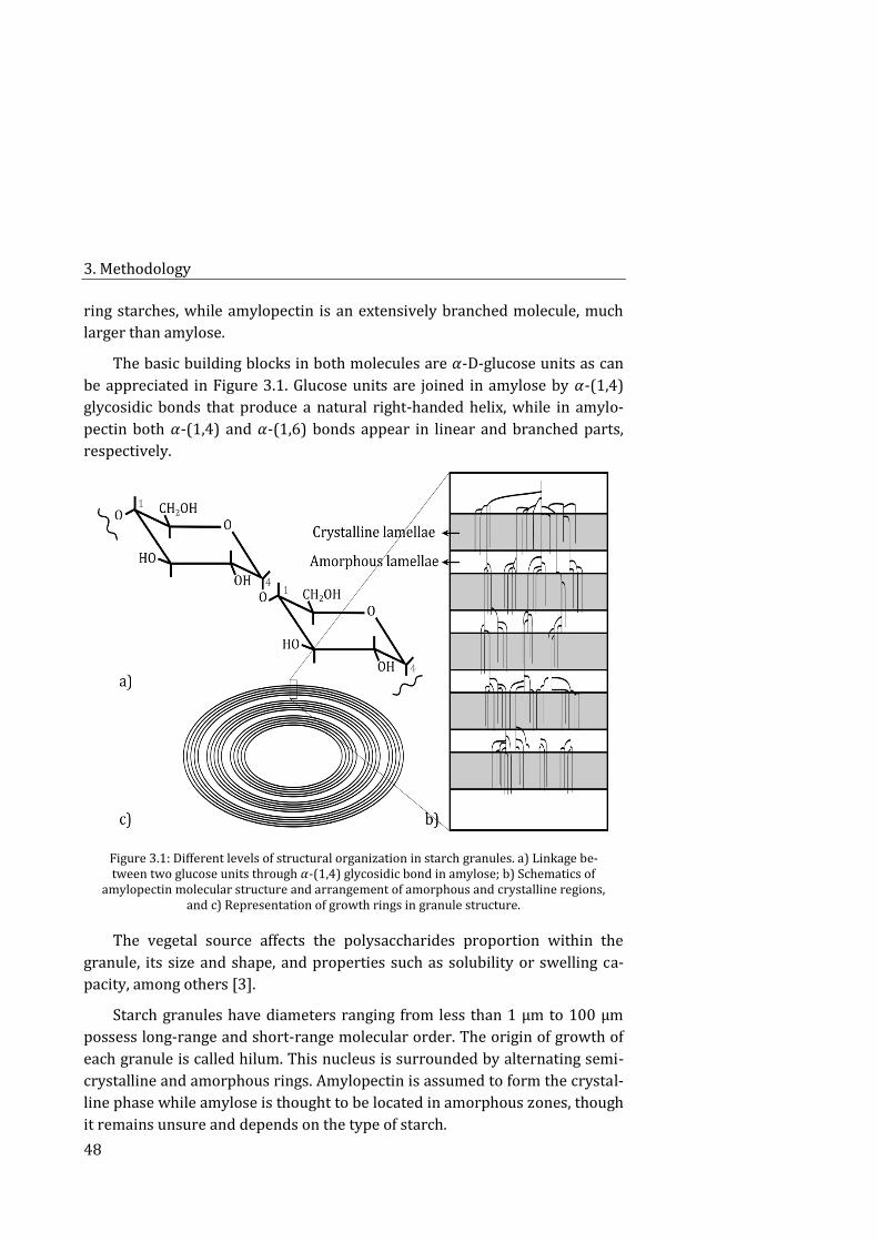
3. Methodology
48
ring starches, while amylopectin is an extensively branched molecule, much
larger than amylose.
The basic building blocks in both molecules are 𝛼-D-glucose units as can
be appreciated in Figure 3.1. Glucose units are joined in amylose by 𝛼-(1,4)
glycosidic bonds that produce a natural right-handed helix, while in amylo-
pectin both 𝛼-(1,4) and 𝛼-(1,6) bonds appear in linear and branched parts,
respectively.
Figure 3.1: Different levels of structural organization in starch granules. a) Linkage be-tween two glucose units through 𝛼-(1,4) glycosidic bond in amylose; b) Schematics of
amylopectin molecular structure and arrangement of amorphous and crystalline regions, and c) Representation of growth rings in granule structure.
The vegetal source affects the polysaccharides proportion within the
granule, its size and shape, and properties such as solubility or swelling ca-
pacity, among others [3].
Starch granules have diameters ranging from less than 1 µm to 100 µm
possess long-range and short-range molecular order. The origin of growth of
each granule is called hilum. This nucleus is surrounded by alternating semi-
crystalline and amorphous rings. Amylopectin is assumed to form the crystal-
line phase while amylose is thought to be located in amorphous zones, though
it remains unsure and depends on the type of starch.
3.1. Materials
49
The granule structure provides information on its swelling capacity.
When granules are heated in excess of water, they expand their volume as a
consequence of water absorption. This swelling process mainly takes place in
the amorphous zones of the granule, so that a part of the amylose molecules is
released into the medium increasing the viscosity. This irreversible loss in the
granular/molecular order is called gelatinization, which is marked by the dis-
appearance of birefringence and in native starches occurs at a range of tem-
perature between 55 and 80 ˚C depending on the botanical source [1]. More-
over, if the sample is subjected to shear the swollen starch granules disinte-
grate forming a paste. When this paste is cooled retrogradation takes place,
i.e., amylose molecules associate again and a three-dimensional network is
formed.
Physically or chemically modified starches appeared in order to improve
their native performance in diverse applications. Their functionalization ena-
bles for example a better stability or change the solubility in cold water. The
first modified starches of which there is evidence were produced by Kirchoff
in 1811 when performed the hydrolysis of potato starch with acid, transform-
ing starch into a sweet substance [4]. An extensive description of modified
starches can be found elsewhere [1,4].
Although most applications of starches involve their heating in presence
of water, where the granular structure is destroyed, it is very conspicuous
their behaviour in water at room temperature and at high concentrations.
These concentrated suspensions are one common example of the counter-
intuitive shear-thickening phenomenon, basically characterized by an in-
crease in viscosity under shear stress or shear rate.
Cornstarch particles have been used along this thesis within several types
of suspensions:
- Concentrated suspensions in water (Chapter 4): the study of the rheo-
logical behaviour is carried out in several geometries as well as the evolu-
tion of normal forces during the shear-thickening range.
- As part of the carrier fluid in the formulation of magnetorheological
shear-thickening fluids (Chapter 5): the addition of starch particles to the
MR fluid permits a considerable reduction in weight for a given volume
fraction, and under the application of a magnetic field the appearance of
the shear-thickening behaviour can be easily tuned.
3. Methodology
50
- Cornstarch was also used as organic coating for carbonyl iron particles
(Chapter 5). The effect of the coating in the rheological behaviour of sus-
pensions formulated with these core-shell particles was studied.
- Suspensions in several carrier fluids (Chapters 6 and 7), to study their
effect in the shear-thickening response and their tribological behaviour.
In these sense, the physical and chemical interactions among particles
and carrier fluid play an important role in the appearance or inhibition of
the shear-thickening phenomenon.
Fumed silica 3.1.2.
Fumed silica (FS) is a white powder with a very high fineness that is obtained
through continuous flame hydrolysis [5,6]. In this synthesis process evapo-
rated silicon tetrachloride SiCl4 reacts with hydrogen H2 and oxygen O2 to be
converted into amorphous silicon dioxide SiO2, and the only by-product being
hydrogen chloride HCl.
Silica, especially fumed silica, is well known for its ability to increase the
viscosity of suspensions in organic media [7–10]. When this material is dis-
persed in the carrier fluid their silanol groups (Si-OH) interact with other si-
lanol groups through hydrogen bonding, both directly and by means of the
solvent molecules. It causes the formation of a three-dimensional network
that upon certain conditions gives rise to the appearance of shear thickening.
This material was used in the formulation of ethylene glycol-based con-
centrated suspensions, and their rheological behaviour will be studied in
Chapter 4 as complement to unimodal suspensions showing shear-thickening
response under certain circumstances. Moreover, dispersions of FS were pre-
pared as model shear-thickening fluids and tribologically characterized in
Chapter 6.
Carbonyl iron 3.1.3.
Carbonyl iron (CI) is produced by thermal decomposition of iron pentacar-
bonyl (Fe(CO)5). The synthesis conditions employed during this process con-
trol the particle properties and so determine the type of powder grade. A
broad spectrum of carbonyl iron grades are commercialized; they are charac-
terized by a given particle size distribution, a particular coating or not, and
different properties according to the requirements of each final application.
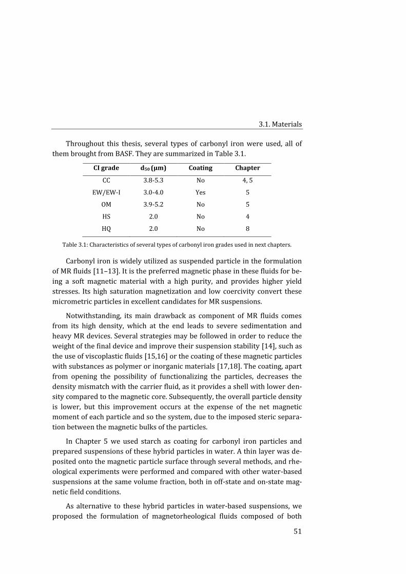
3.1. Materials
51
Throughout this thesis, several types of carbonyl iron were used, all of
them brought from BASF. They are summarized in Table 3.1.
CI grade d50 (μm) Coating Chapter
CC 3.8-5.3 No 4, 5
EW/EW-I 3.0-4.0 Yes 5
OM 3.9-5.2 No 5
HS 2.0 No 4
HQ 2.0 No 8
Table 3.1: Characteristics of several types of carbonyl iron grades used in next chapters.
Carbonyl iron is widely utilized as suspended particle in the formulation
of MR fluids [11–13]. It is the preferred magnetic phase in these fluids for be-
ing a soft magnetic material with a high purity, and provides higher yield
stresses. Its high saturation magnetization and low coercivity convert these
micrometric particles in excellent candidates for MR suspensions.
Notwithstanding, its main drawback as component of MR fluids comes
from its high density, which at the end leads to severe sedimentation and
heavy MR devices. Several strategies may be followed in order to reduce the
weight of the final device and improve their suspension stability [14], such as
the use of viscoplastic fluids [15,16] or the coating of these magnetic particles
with substances as polymer or inorganic materials [17,18]. The coating, apart
from opening the possibility of functionalizing the particles, decreases the
density mismatch with the carrier fluid, as it provides a shell with lower den-
sity compared to the magnetic core. Subsequently, the overall particle density
is lower, but this improvement occurs at the expense of the net magnetic
moment of each particle and so the system, due to the imposed steric separa-
tion between the magnetic bulks of the particles.
In Chapter 5 we used starch as coating for carbonyl iron particles and
prepared suspensions of these hybrid particles in water. A thin layer was de-
posited onto the magnetic particle surface through several methods, and rhe-
ological experiments were performed and compared with other water-based
suspensions at the same volume fraction, both in off-state and on-state mag-
netic field conditions.
As alternative to these hybrid particles in water-based suspensions, we
proposed the formulation of magnetorheological fluids composed of both
3. Methodology
52
magnetic and non-magnetic particles. The idea of this hybrid system is based
on recent works [19–21] where it has been shown that the partial substitu-
tion of magnetic particles by non-magnetic ones results in an improved mag-
netic response, i.e., a higher yield stress for the same volume fraction com-
pared to the unimodal case of a conventional MR fluid.
If these non-magnetic particles form part of the carrier fluid, its viscosity
would be a function of the particle concentration. Moreover, a higher viscosity
would inhibit particle sedimentation and magnetic aggregation in no-field
conditions. In this manner, a required yield stress for a specific application
could be obtained in a suspension with a lower concentration of carbonyl
iron, with the subsequent reduction in weight and cost, and improved particle
stability.
We selected starch as non-magnetic particle so that the carrier fluid may
show shear-thickening response under adequate circumstances. In this sense,
the addition of carbonyl iron particles to a shear-thickening suspension re-
sults in a fluid with both shear-thickening and magnetic characteristics. Thus,
the appearance of shear-thickening behaviour will depend on the applied
magnetic field, particle concentration, range of shear rates and the interac-
tions between starch and the fluid. These types of suspensions are called
magnetorheological shear-thickening (MRST) fluids.
Sample preparation 3.1.4.
Starch suspensions
In these experiments starch from corn (S4126, containing a 27% of amylose
and a 73% of amylopectin) from Sigma Aldrich was used, and suspended at
the required volume fractions in distinct carrier fluids, whose properties are
shown in Table 3.2. Native starch granules have irregular faceted shape as can
be observed onwards in the ESEM micrographs (see Subsection 3.2.3). The
mean particle diameter was 10.7 μm.
Suspensions were prepared in plastic containers by weighting the re-
quired amount of cornstarch and carrier fluid. Then, both components were
carefully and manually mixed with a spatula to ensure a homogeneous distri-
bution of particles within the sample. This procedure was of special im-
portance when working at high particle concentrations, for which rapid
movements (high stresses) would entail the thickening of the sample and the
development of normal stresses, so that some time would be needed for their
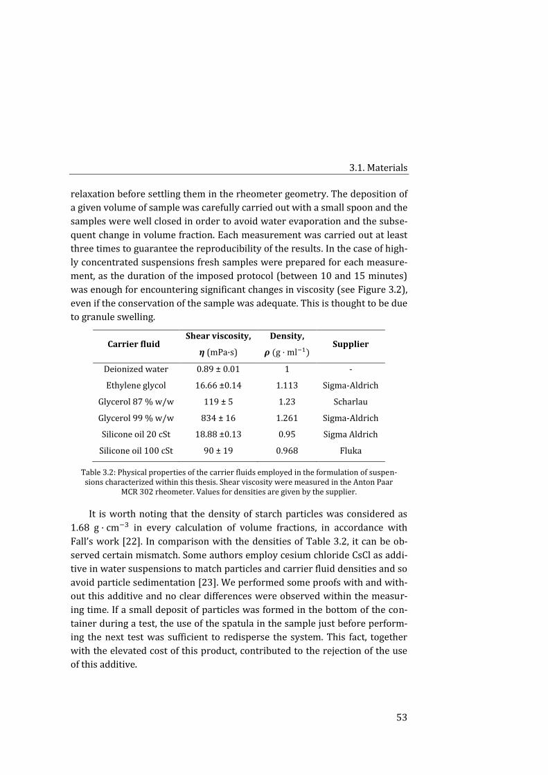
3.1. Materials
53
relaxation before settling them in the rheometer geometry. The deposition of
a given volume of sample was carefully carried out with a small spoon and the
samples were well closed in order to avoid water evaporation and the subse-
quent change in volume fraction. Each measurement was carried out at least
three times to guarantee the reproducibility of the results. In the case of high-
ly concentrated suspensions fresh samples were prepared for each measure-
ment, as the duration of the imposed protocol (between 10 and 15 minutes)
was enough for encountering significant changes in viscosity (see Figure 3.2),
even if the conservation of the sample was adequate. This is thought to be due
to granule swelling.
Carrier fluid Shear viscosity,
𝜼 (mPa·s)
Density,
𝝆 (g · ml−1) Supplier
Deionized water 0.89 ± 0.01 1 -
Ethylene glycol 16.66 ±0.14 1.113 Sigma-Aldrich
Glycerol 87 % w/w 119 ± 5 1.23 Scharlau
Glycerol 99 % w/w 834 ± 16 1.261 Sigma-Aldrich
Silicone oil 20 cSt 18.88 ±0.13 0.95 Sigma Aldrich
Silicone oil 100 cSt 90 ± 19 0.968 Fluka
Table 3.2: Physical properties of the carrier fluids employed in the formulation of suspen-sions characterized within this thesis. Shear viscosity were measured in the Anton Paar
MCR 302 rheometer. Values for densities are given by the supplier.
It is worth noting that the density of starch particles was considered as
1.68 g · cm−3 in every calculation of volume fractions, in accordance with
Fall’s work [22]. In comparison with the densities of Table 3.2, it can be ob-
served certain mismatch. Some authors employ cesium chloride CsCl as addi-
tive in water suspensions to match particles and carrier fluid densities and so
avoid particle sedimentation [23]. We performed some proofs with and with-
out this additive and no clear differences were observed within the measur-
ing time. If a small deposit of particles was formed in the bottom of the con-
tainer during a test, the use of the spatula in the sample just before perform-
ing the next test was sufficient to redisperse the system. This fact, together
with the elevated cost of this product, contributed to the rejection of the use
of this additive.
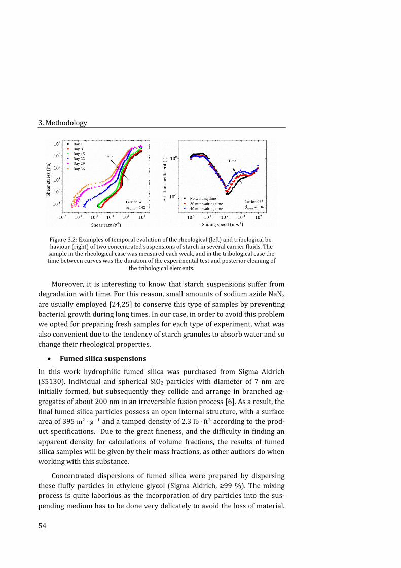
3. Methodology
54
Figure 3.2: Examples of temporal evolution of the rheological (left) and tribological be-haviour (right) of two concentrated suspensions of starch in several carrier fluids. The
sample in the rheological case was measured each weak, and in the tribological case the time between curves was the duration of the experimental test and posterior cleaning of
the tribological elements.
Moreover, it is interesting to know that starch suspensions suffer from
degradation with time. For this reason, small amounts of sodium azide NaN3
are usually employed [24,25] to conserve this type of samples by preventing
bacterial growth during long times. In our case, in order to avoid this problem
we opted for preparing fresh samples for each type of experiment, what was
also convenient due to the tendency of starch granules to absorb water and so
change their rheological properties.
Fumed silica suspensions
In this work hydrophilic fumed silica was purchased from Sigma Aldrich
(S5130). Individual and spherical SiO2 particles with diameter of 7 nm are
initially formed, but subsequently they collide and arrange in branched ag-
gregates of about 200 nm in an irreversible fusion process [6]. As a result, the
final fumed silica particles possess an open internal structure, with a surface
area of 395 m2 · g−1 and a tamped density of 2.3 lb · ft3 according to the prod-
uct specifications. Due to the great fineness, and the difficulty in finding an
apparent density for calculations of volume fractions, the results of fumed
silica samples will be given by their mass fractions, as other authors do when
working with this substance.
Concentrated dispersions of fumed silica were prepared by dispersing
these fluffy particles in ethylene glycol (Sigma Aldrich, ≥99 %). The mixing
process is quite laborious as the incorporation of dry particles into the sus-
pending medium has to be done very delicately to avoid the loss of material.
3.1. Materials
55
The shear-thickening behaviour of these samples was studied in wide range
of concentrations.
On the other hand, fumed silica was employed in dispersions with differ-
ent mixtures of water and glycerol in order to study the effect of the carrier
fluid in their shear-thickening and tribological response.
MR suspensions
In Chapter 4 concentrated MR suspensions were investigated. They were
prepared by dispersing carbonyl iron (EW grade, from BASF SE, Germany) in
four carrier fluids, namely ethylene glycol, glycerol 87 %w/w, and silicone oil
with viscosities of 20 cSt and 100 cSt (see Table 3.2). These suspensions
combine a magnetic response upon the application of a given magnetic field
strength and certain shear-thickening character, due to their high particle
concentration, which depends on the physicochemical properties of the carri-
er fluid.
However, in squeeze experiments conventional MR suspensions of car-
bonyl iron (grade HQ, from BASF SE, Germany) in silicone oil were studied
(Chapter 8). The concentration was a 5 % in order to compare with previous
squeeze results on diluted samples [26].
The preparation of these types of samples involved the simple mixing of
both components with the spatula, the use of ultrasounds in order to disrupt
magnetic aggregates as well as the planetary mixer, where the particles be-
come homogeneously distributed within the suspension. These two steps
were carried out before each measurement due to particle sedimentation.
MRST suspensions
In Chapter 5 we studied the rheological behaviour of hybrid suspensions with
magnetic and shear-thickening character. Two approaches were performed:
by means of suspending a mixture of magnetic (carbonyl iron, CC grade) and
non-magnetic particles (starch) in water, and on the other hand by using
starch-coated carbonyl iron particles (EW and HS grades) suspended in wa-
ter.
These MRST suspensions were easily prepared as for MR suspensions.
3. Methodology
56
Experimental methods 3.2.
Rheometry 3.2.1.
The measurement of the rheological material functions is called rheometry.
Rheological experiments provide the relationship between applied stresses
and deformations in a material and can be performed in shear or extensional
rheometers [27]. Most rheological measurements are carried out in shear ge-
ometries where experimentation is easier. However, the generation and
measurement of homogeneous extensional flows have many practical difficul-
ties and thus extensional rheometers are less developed. Shear flow is typical-
ly used when the viscosity is the main material property. Other classification
of flows is by the use of small or large strains, as well as by transient or steady
flows.
The stress responses of a given material under study depend both on the
nature of the material and the type of flow imposed to it. Shear rheometers
can be divided into two groups: drag flows and driven flows. In drag flow the
shear is generated between a moving and a fixed solid surface. Sliding plates,
concentric cylinders (Couette flow), cone and plate, and parallel disks are ge-
ometries belonging to drag flows. Rotational instruments may be operated in
the steady shear (constant angular velocity) or oscillatory (dynamic) mode.
On the other hand, capillary geometry (Poiseuille flow), slit flow and axial an-
nular flow are types of pressure flows, where a pressure difference over a
close channel, through which the material flows, is responsible for generating
the shear. Other popular pressure-driven flow can also be produced by means
of the squeezing flow between parallel plates.
Extensional flows by their part, exhibit very sensitive variations in struc-
ture and this type of deformation play a significant role in some industrial
processes as fibre spinning flows. When a given material is subjected to ex-
tensional flows the material is stretched along streamlines. In fact, stretching
occurs with all deformations but stretching in shear is only observed between
particles in different streamlines.
The choice of a measuring system depends on the nature of the studied
sample and determines the shear stress and shear rate ranges. The most
commonly used devices within this thesis are cone-plate and plate-plate ge-
ometries. The main characteristics of each geometry are shown below:
3.2. Experimental methods
57
- In cone-plate geometry the shear rate and stress are homogeneous in
the whole gap, so that the viscosity is independent of the measuring
point. For this assertion to be valid the angle of the cone has to be
very small as it will be explained later in conversion of data. It re-
quires small volumes of samples and is used in normal force meas-
urements. The cone is truncated and the gap is fixed at a distance
from the plate, and this fact restricts the type of sample that can be
used within this geometry. In this sense, the particle diameter has to
be below a tenth of the gap.
- Parallel plates enable the variation of the gap size and so the attaina-
ble shear rates the sample is subjected to. In the same manner the
larger the plate radius, the larger the feasible shear rates. Moreover
serrated plates can be used to avoid slippage.
In next sections, the rheological characterization of our complex fluids,
which were carried out in torsional and squeeze modes in an Anton Paar
magnetorheometer (MCR 501, MRD70-SN81112937), is described. Then the
equations relating the raw data from the rheometer and shear stresses and
strains are exposed. After that attention will also be paid to the quantification
of normal stresses that may appear in our systems during the rheological
measurements. At the end of this subsection we will take into account some
considerations in the determination of yield stresses and the correction of a
very important experimental artefact as wall slip.
Torsional experiments
Small-angle cone-plate and plate-plate geometries have been employed in
torsional experiments. Both geometries are traditionally used in rheological
measurements of complex fluids.
The rheological characterization of concentrated starch (or silica) sus-
pensions was principally performed with parallel plates, except for the de-
termination of the normal force, for which the cone-plate measuring system
was used. In the case of mixtures of magnetic and non-magnetic particles as
well as for concentrated MR suspensions of carbonyl iron, the rheological
measurements were carried out in parallel plates, as they allow for the appli-
cation of an external magnetic field and a uniform distribution within the gap.
Squeeze experiments
Squeeze experiments were used in Chapter 8 to study the squeeze strength-
ening effect in MR suspensions of carbonyl iron in silicone oil. Squeeze con-
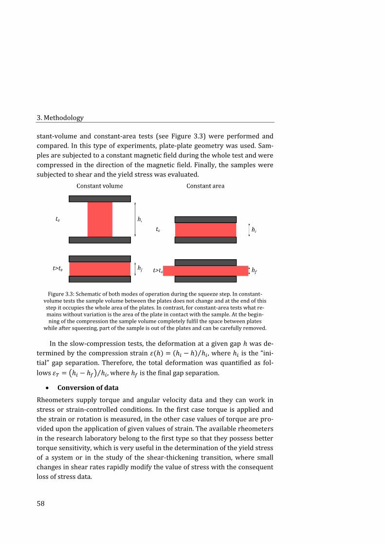
3. Methodology
58
stant-volume and constant-area tests (see Figure 3.3) were performed and
compared. In this type of experiments, plate-plate geometry was used. Sam-
ples are subjected to a constant magnetic field during the whole test and were
compressed in the direction of the magnetic field. Finally, the samples were
subjected to shear and the yield stress was evaluated.
Figure 3.3: Schematic of both modes of operation during the squeeze step. In constant-volume tests the sample volume between the plates does not change and at the end of this step it occupies the whole area of the plates. In contrast, for constant-area tests what re-mains without variation is the area of the plate in contact with the sample. At the begin-ning of the compression the sample volume completely fulfil the space between plates
while after squeezing, part of the sample is out of the plates and can be carefully removed.
In the slow-compression tests, the deformation at a given gap ℎ was de-
termined by the compression strain 휀(ℎ) = (ℎ𝑖 − ℎ) ℎ𝑖⁄ , where ℎ𝑖 is the “ini-
tial” gap separation. Therefore, the total deformation was quantified as fol-
lows 휀𝑇 = (ℎ𝑖 − ℎ𝑓) ℎ𝑖⁄ , where ℎ𝑓 is the final gap separation.
Conversion of data
Rheometers supply torque and angular velocity data and they can work in
stress or strain-controlled conditions. In the first case torque is applied and
the strain or rotation is measured, in the other case values of torque are pro-
vided upon the application of given values of strain. The available rheometers
in the research laboratory belong to the first type so that they possess better
torque sensitivity, which is very useful in the determination of the yield stress
of a system or in the study of the shear-thickening transition, where small
changes in shear rates rapidly modify the value of stress with the consequent
loss of stress data.
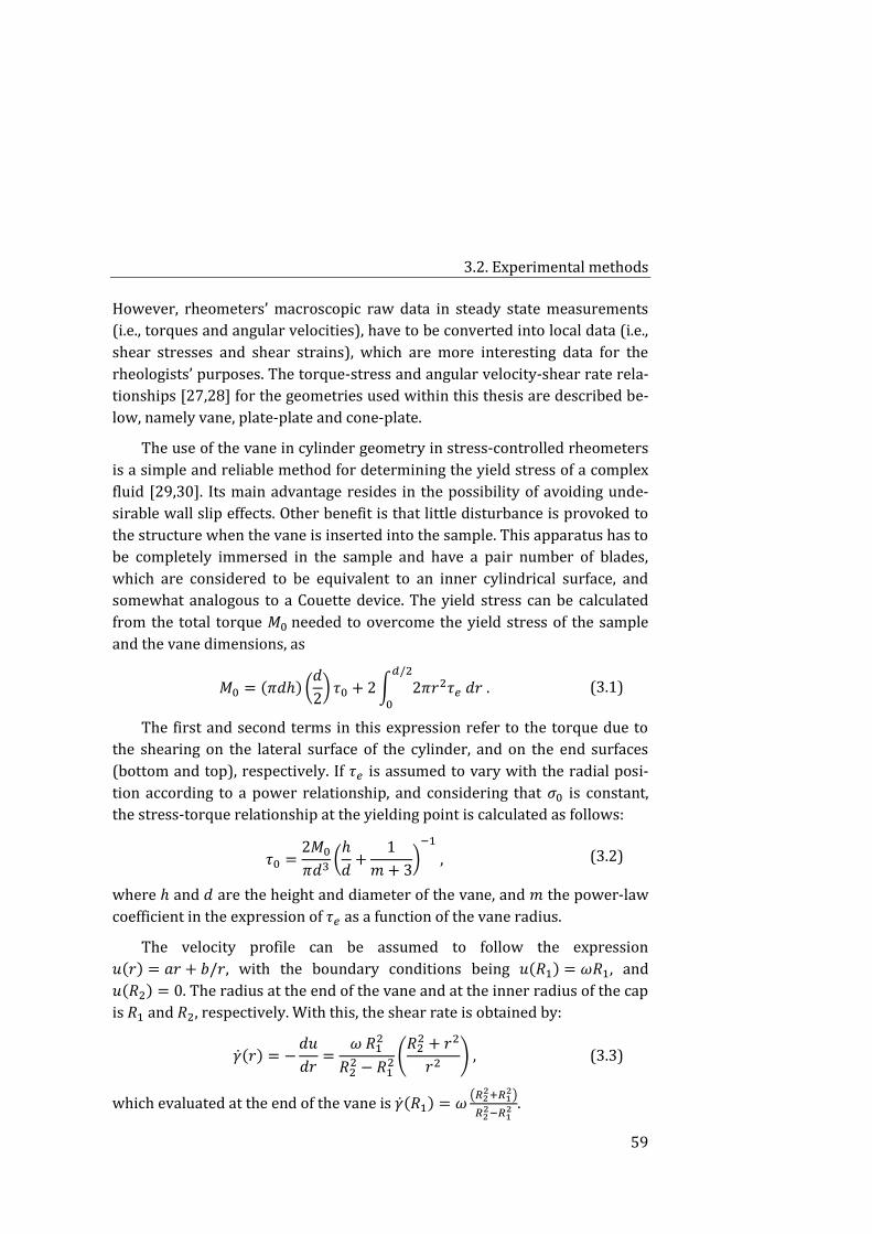
3.2. Experimental methods
59
However, rheometers’ macroscopic raw data in steady state measurements
(i.e., torques and angular velocities), have to be converted into local data (i.e.,
shear stresses and shear strains), which are more interesting data for the
rheologists’ purposes. The torque-stress and angular velocity-shear rate rela-
tionships [27,28] for the geometries used within this thesis are described be-
low, namely vane, plate-plate and cone-plate.
The use of the vane in cylinder geometry in stress-controlled rheometers
is a simple and reliable method for determining the yield stress of a complex
fluid [29,30]. Its main advantage resides in the possibility of avoiding unde-
sirable wall slip effects. Other benefit is that little disturbance is provoked to
the structure when the vane is inserted into the sample. This apparatus has to
be completely immersed in the sample and have a pair number of blades,
which are considered to be equivalent to an inner cylindrical surface, and
somewhat analogous to a Couette device. The yield stress can be calculated
from the total torque 𝑀0 needed to overcome the yield stress of the sample
and the vane dimensions, as
𝑀0 = (𝜋𝑑ℎ) (𝑑
2) 𝜏0 + 2 ∫ 2𝜋𝑟2𝜏𝑒 𝑑𝑟
𝑑/2
0
. (3.1)
The first and second terms in this expression refer to the torque due to
the shearing on the lateral surface of the cylinder, and on the end surfaces
(bottom and top), respectively. If 𝜏𝑒 is assumed to vary with the radial posi-
tion according to a power relationship, and considering that 𝜎0 is constant,
the stress-torque relationship at the yielding point is calculated as follows:
𝜏0 =2𝑀0
𝜋𝑑3(
ℎ
𝑑+
1
𝑚 + 3)
−1
, (3.2)
where ℎ and 𝑑 are the height and diameter of the vane, and 𝑚 the power-law
coefficient in the expression of 𝜏𝑒 as a function of the vane radius.
The velocity profile can be assumed to follow the expression
𝑢(𝑟) = 𝑎𝑟 + 𝑏/𝑟, with the boundary conditions being 𝑢(𝑅1) = 𝜔𝑅1, and
𝑢(𝑅2) = 0. The radius at the end of the vane and at the inner radius of the cap
is 𝑅1 and 𝑅2, respectively. With this, the shear rate is obtained by:
�̇�(𝑟) = −𝑑𝑢
𝑑𝑟=
𝜔 𝑅12
𝑅22 − 𝑅1
2 (𝑅2
2 + 𝑟2
𝑟2 ) , (3.3)
which evaluated at the end of the vane is �̇�(𝑅1) = 𝜔(𝑅2
2+𝑅12)
𝑅22−𝑅1
2 .
3. Methodology
60
In parallel plates geometry, the shear rate is again proportional to the an-
gular velocity 𝜔 at which the upper plate moves as a consequence of the ap-
plied torque, and a function of the radius:
�̇� = 𝑓(𝑟) =𝜔𝑟
ℎ , �̇�𝑅 =
𝜔𝑅
ℎ , (3.4)
where 𝑅 is the radius of the plate and ℎ the gap between plates.
Shear stress in parallel plates, in contrast to the cone-plate geometry, is a
function of the radius (𝜏 = 𝑓(�̇�)) and has to be determined by integrating a
force balance equation over the radius:
∫ 𝑑𝑀 = 𝑀
0
2𝜋 ∫ (𝑟2𝜏)𝑅
0
𝑑𝑟 . (3.5)
Changing the limits of integration, substituting the radius by the expres-
sion of shear rate, and since the shear stress is function of shear rate, the
equation can be written as
𝑀(�̇�𝑅)3
2𝜋𝑅3= ∫ (�̇�)2𝑓
�̇�𝑅
0
(�̇�)𝑑�̇� . (3.6)
If the equation is differentiated with respect to the shear rate at the rim
the Leibnitz’ rule may be applied. It allows the integral in the right term (with
the form of 𝑑
𝑑𝑧′[∫ 𝑧2𝑓
𝑧′
0(𝑧)𝑑𝑧]) to be written as �̇�𝑅
2𝑓(�̇�𝑅). The expression for
the shear stress at the rim of the plate is thus obtained as follows:
𝜏𝑅 = 𝑓(�̇�) =𝑀
2𝜋𝑅3(3 +
𝑑 ln 𝑀
𝑑 ln �̇�) . (3.7)
This equation is similar to Rabinowitsch-Mooney equation, where the
shear rate is expressed as a function of the shear stress, �̇� = 𝑓(𝜏). If the law
relating shear rate and stress is known, which depends on the type of fluid
behaviour, the relationship between torque and the angular velocity can be
easily obtained. The derivative in the right side of the equation can be calcu-
lated by data analysis software and the calculation of shear stress at the rim is
thus straightforward.
When cone-plate geometry is used the transformation of raw data from
the rheometer into shear stress and rate in the sample is simple:
𝜏 =3𝑀
2𝜋𝑅3 . (3.8)
3.2. Experimental methods
61
The expression for the shear rate in cone-plate geometry is similar to(3.4,
the analogous in plate-plate geometry:
ℎ
𝑅= tan 𝛼𝑟𝑎𝑑 ≈ 𝛼𝑟𝑎𝑑 → �̇�𝑅 ≈
𝜔
𝛼𝑟𝑎𝑑 . (3.9)
The angle of the cone tool 𝛼𝑟𝑎𝑑 is usually very small, and from trigonome-
try, the ratio between the gap ℎ and the radius of the cone 𝑅 coincides with
the tangent of this angle. For angles tending to zero this tangent can be ap-
proximated, with an acceptable accuracy, to the angle expressed in radians.
Normal stress differences
Differences between normal components (𝜏𝑥𝑥, 𝜏𝑦𝑦, 𝜏𝑧𝑧) are consequences of
microstructure anisotropy, and result in deformation when they are distinct
from zero. The first normal stress difference (𝑁1 = 𝜏𝑥𝑥 − 𝜏𝑦𝑦) can be directly
obtained in rheological measurements when the test is performed with a
cone-plate geometry. The total thrust 𝐹𝑁 in cone-plate geometry (a normal
force acting on the upper tool, the cone) can be easily transformed in this pa-
rameter (𝑁1 =2𝐹𝑁
𝜋𝑅2). Once the value of 𝑁1 is known the second normal stress
difference (𝑁2 = 𝜏𝑦𝑦 − 𝜏𝑧𝑧) can be calculated from plate-plate measurements.
The thrust measured in this geometry can be related with the difference be-
tween both quantities in this form [31]:
𝑁1(�̇�𝑅) − 𝑁2(�̇�𝑅) =𝐹𝑁
𝜋𝑅2(2 +
𝑑 ln 𝐹𝑁
𝑑 ln �̇�𝑅) . (3.10)
The normal stress determined from parallel plates data is generally a
good approximation of the first normal stress difference, as the second one is
usually very small compared to the former.
Thus, changes in normal stress differences during a rheological test in-
volve changes in the sample microstructure and provide useful information
about the sample behaviour. For instance, Royer et al. [10] studied concen-
trated non-colloidal suspensions formulated with silica particles under shear
and observed a clear transition of 𝑁1 from negative to positive values devel-
oped by the sample, as the particle concentration increase. For diluted sam-
ples the first normal stress difference remains negative as a consequence of
the prevalence of hydrodynamic forces due to shear compared to Brownian
ones. However, for higher concentrations at low values of shear stress hydro-
dynamic forces again dominate over other forces, while at higher shear
stresses contact forces and frictional interactions prevail over hydrodynamic
3. Methodology
62
ones, resulting in positive first normal stress differences. From the macro-
scopic point of view, these positive values reflect dilatancy, a volume expan-
sion that in a confined system give rise to the appearance of shear-thickening
behaviour.
Yield stress measurements
Many complex fluids are characterized by an apparent yield stress, a rheolog-
ical property by which a material flows when the applied stress exceeds a
particular value, and below this stress the material elastically deforms. Con-
centrated suspensions with strong interparticle interactions often exhibit this
yielding behaviour. These fluids have a structural skeleton which breaks in
the yield stress. It is the case of many shear thinning fluids as daily products
(toothpaste and ketchup), and of relevance within this thesis in MR fluids,
where field induced yield stress is found [32–34].
In the classical description given by Bingham the critical value separates
a region in the rheogram with infinite viscosity from other where the stress
monotonically increases with the shear rate, so that the transition from solid
to liquid state would occur at a unique value of stress. Years later Barnes and
Walters [35] asserted that the yield stress was an artefact and that fluids ca-
pable of flowing at high stresses would also flow at all lower values, for which
viscosity would be very high but not infinite. This work brought many reac-
tions from other colleges and nowadays there is still controversy about the
existence of a true yield stress [36–38]. Despite this, it is undeniable the use-
fulness of the concept of yield stress and yield-stress equations in numerous
applications.
In practice, there is no a reliable method for determining the yield stress,
which often results affected by the technique employed and thixotropic ef-
fects of the sample. Experimentalists observe small shear rates variations up-
on the application of small values of stress, instead of a completely static situ-
ation below the apparent yield stress. For many fluids there is a competition
between aging and rejuvenation processes, two phenomena describing the
spontaneous build-up occurring in the microstructure at rest and the break-
age in flow conditions, respectively.
Yield stress fluids can be categorized into simple yield stress fluids and
thixotropic yield stress fluids [39,40]. The former type corresponds to fluids
for which the shear stress is only dependent on the shear rate and not on the
shear history of the sample. Nevertheless, in thixotropic yield stress fluids the
3.2. Experimental methods
63
flow history is very important: if an up-and-down stress ramp is performed
with these fluids, the static and dynamic yield stresses will differ as the vis-
cosity of the sample is reduced with time. Static yield stress is defined then as
the stress above which the material starts to flow when starting from rest and
the dynamic one is the stress at which the transition from liquid to solid takes
place, so that the sample is subjected to a diminishing stress ramp up to it
completely ceases its flow. However, for simple yield stress fluids the deter-
mination of the yield stress is easier as both static and dynamic yield stresses
coincide. As an example of the rheological behaviour of these two types of
yielding fluids subjected to consecutive up and down stress ramps, the work
of Ovarlez et al. [41] can be consulted, namely in their Figure 2.
Although the determination of yield stress [42] is usually accompanied by
experimental difficulties, it can be performed through several approaches. In
order to obtain reliable yield stress measurements the test type has to be
carefully selected. Among them stress ramp, stress growth, oscillation ampli-
tude sweep and multiple creep are the easiest methods to perform the yield
stress measurements. The choice of the measurement system is also im-
portant as wall slip effects should be avoided. In this sense, the use of rough-
ened surfaces is recommended. When working with a cone-plate geometry
with small cone angle the shear stress can be considered to be homogenously
distributed, so that if the material exhibits yielding flow behaviour, this yield-
ing would be homogeneous whatever the sample radius. Thus, in this case the
cone measuring system would be preferable to parallel plates. However, alt-
hough roughened cones are also available, the last geometry is used if the
suspension is formed by large particles (remember the limitation that the
particle diameter should not be above a tenth of the gap) and when the slip-
page is significant, and serrated plates are used in order to minimize it. More-
over, the vane geometry is a common tool for measuring the yield stress of
structured systems, as this apparatus slightly disturbs the initial structure
when it is inserted into the sample.
Once the rheological measurement has been carried out the value of the
yield stress can be obtained by fitting the data to traditional yield models
such as Bingham, Herschel-Bulkey or Casson equations, and extrapolating the
data to zero shear rate. If the fit is not good enough, a tangent analysis can be
used to extract the yield stress value from the data.
It will be seen in Chapter 8 that the yield stress determination may result
greatly affected by the wall slip phenomenon. Corrections described below
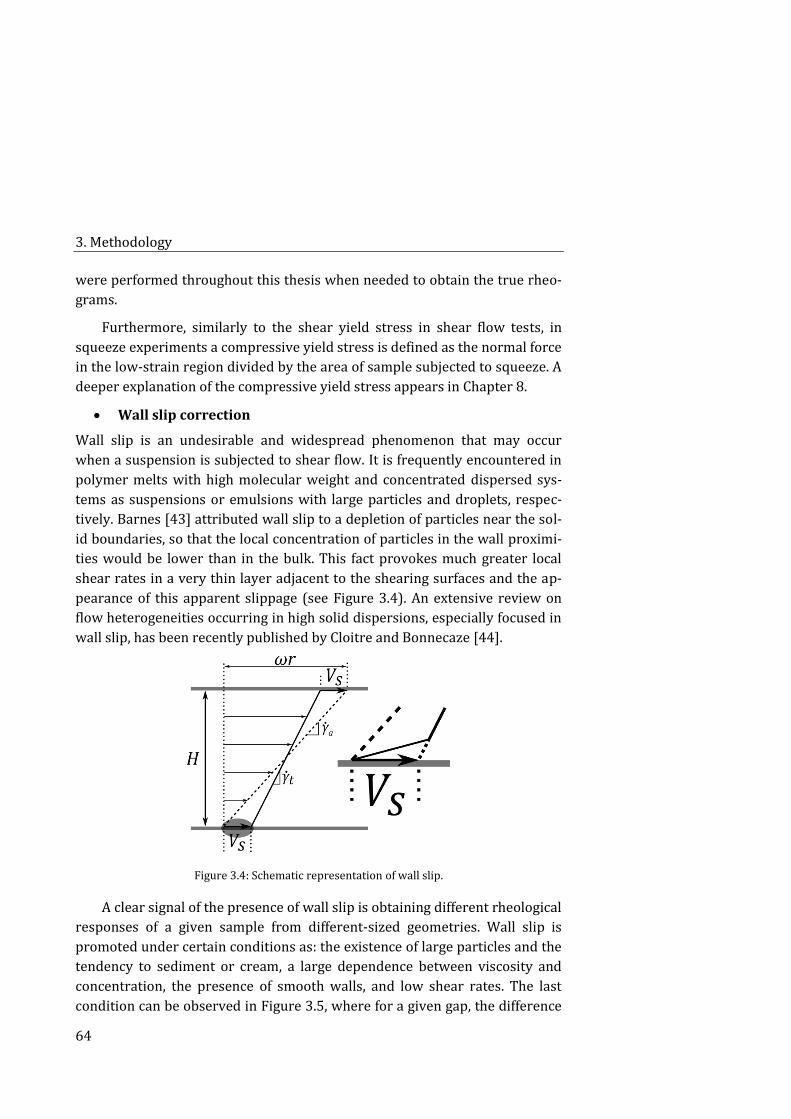
3. Methodology
64
were performed throughout this thesis when needed to obtain the true rheo-
grams.
Furthermore, similarly to the shear yield stress in shear flow tests, in
squeeze experiments a compressive yield stress is defined as the normal force
in the low-strain region divided by the area of sample subjected to squeeze. A
deeper explanation of the compressive yield stress appears in Chapter 8.
Wall slip correction
Wall slip is an undesirable and widespread phenomenon that may occur
when a suspension is subjected to shear flow. It is frequently encountered in
polymer melts with high molecular weight and concentrated dispersed sys-
tems as suspensions or emulsions with large particles and droplets, respec-
tively. Barnes [43] attributed wall slip to a depletion of particles near the sol-
id boundaries, so that the local concentration of particles in the wall proximi-
ties would be lower than in the bulk. This fact provokes much greater local
shear rates in a very thin layer adjacent to the shearing surfaces and the ap-
pearance of this apparent slippage (see Figure 3.4). An extensive review on
flow heterogeneities occurring in high solid dispersions, especially focused in
wall slip, has been recently published by Cloitre and Bonnecaze [44].
Figure 3.4: Schematic representation of wall slip.
A clear signal of the presence of wall slip is obtaining different rheological
responses of a given sample from different-sized geometries. Wall slip is
promoted under certain conditions as: the existence of large particles and the
tendency to sediment or cream, a large dependence between viscosity and
concentration, the presence of smooth walls, and low shear rates. The last
condition can be observed in Figure 3.5, where for a given gap, the difference
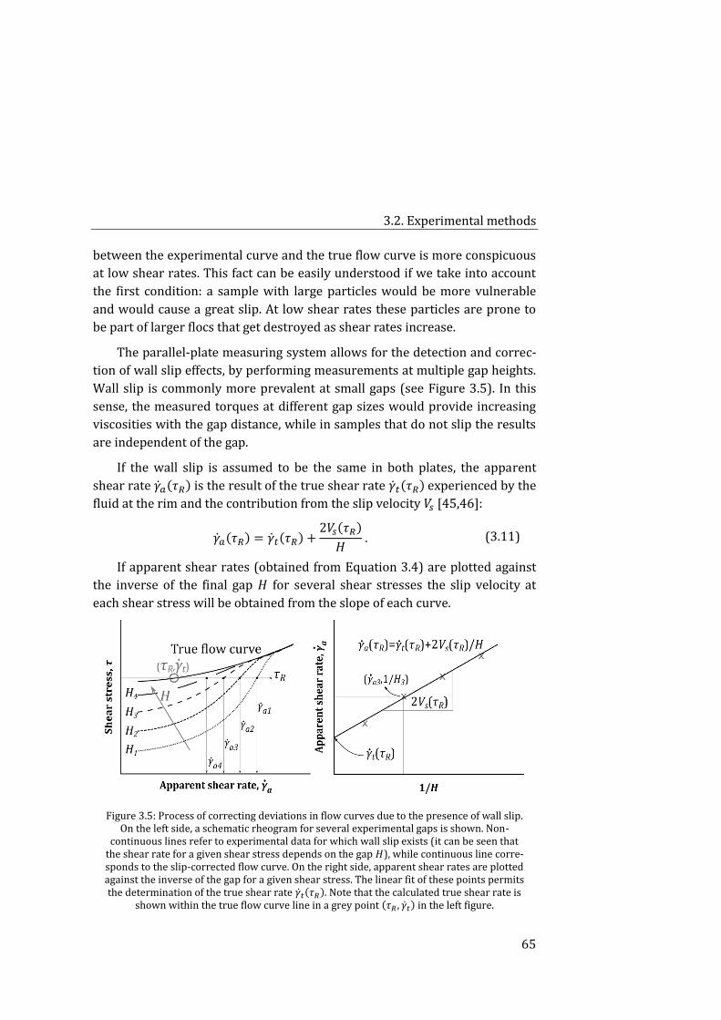
3.2. Experimental methods
65
between the experimental curve and the true flow curve is more conspicuous
at low shear rates. This fact can be easily understood if we take into account
the first condition: a sample with large particles would be more vulnerable
and would cause a great slip. At low shear rates these particles are prone to
be part of larger flocs that get destroyed as shear rates increase.
The parallel-plate measuring system allows for the detection and correc-
tion of wall slip effects, by performing measurements at multiple gap heights.
Wall slip is commonly more prevalent at small gaps (see Figure 3.5). In this
sense, the measured torques at different gap sizes would provide increasing
viscosities with the gap distance, while in samples that do not slip the results
are independent of the gap.
If the wall slip is assumed to be the same in both plates, the apparent
shear rate �̇�𝑎(𝜏𝑅) is the result of the true shear rate �̇�𝑡(𝜏𝑅) experienced by the
fluid at the rim and the contribution from the slip velocity 𝑉𝑠 [45,46]:
�̇�𝑎(𝜏𝑅) = �̇�𝑡(𝜏𝑅) +2𝑉𝑠(𝜏𝑅)
𝐻 . (3.11)
If apparent shear rates (obtained from Equation 3.4) are plotted against
the inverse of the final gap 𝐻 for several shear stresses the slip velocity at
each shear stress will be obtained from the slope of each curve.
Figure 3.5: Process of correcting deviations in flow curves due to the presence of wall slip. On the left side, a schematic rheogram for several experimental gaps is shown. Non-
continuous lines refer to experimental data for which wall slip exists (it can be seen that the shear rate for a given shear stress depends on the gap 𝐻), while continuous line corre-sponds to the slip-corrected flow curve. On the right side, apparent shear rates are plotted against the inverse of the gap for a given shear stress. The linear fit of these points permits the determination of the true shear rate �̇�𝑡(𝜏𝑅). Note that the calculated true shear rate is
shown within the true flow curve line in a grey point (𝜏𝑅 , �̇�𝑡) in the left figure.
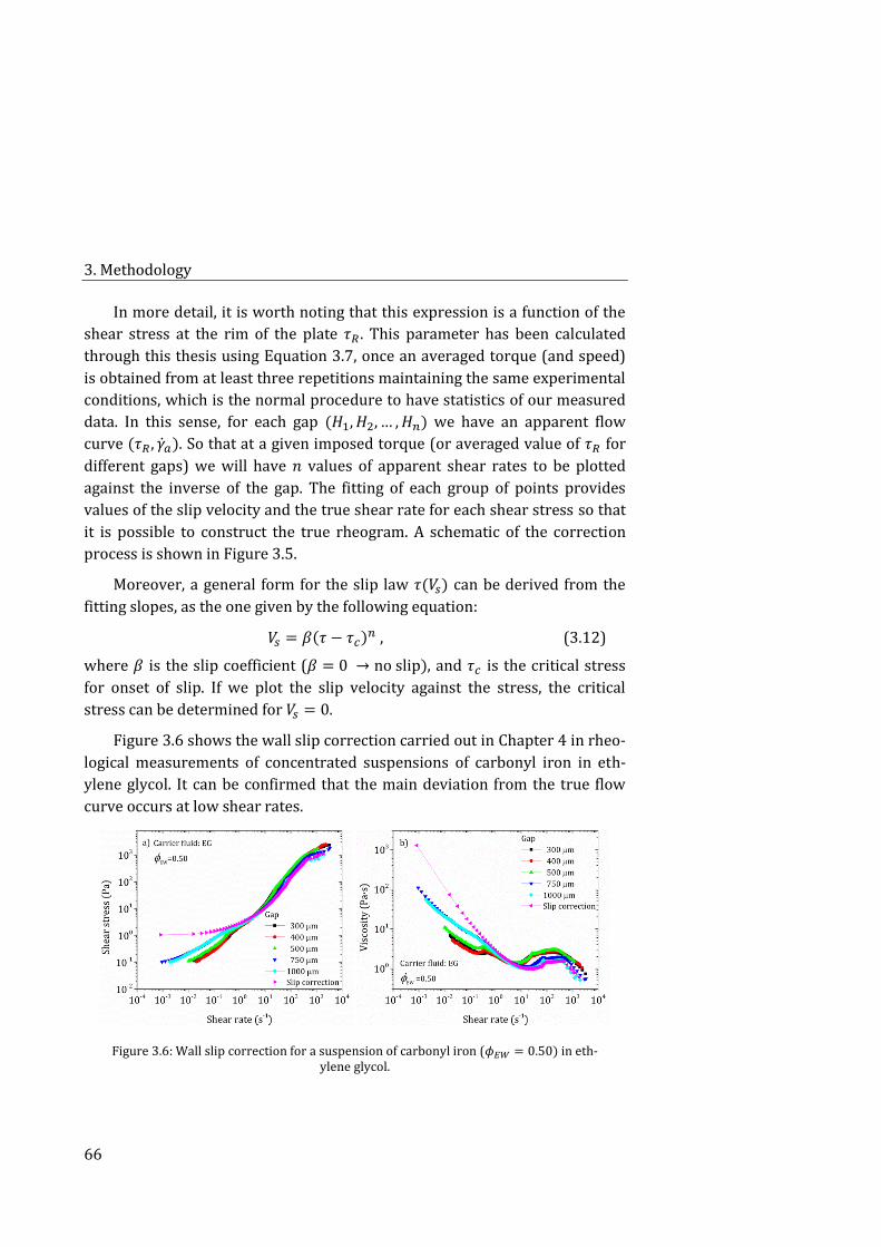
3. Methodology
66
In more detail, it is worth noting that this expression is a function of the
shear stress at the rim of the plate 𝜏𝑅 . This parameter has been calculated
through this thesis using Equation 3.7, once an averaged torque (and speed)
is obtained from at least three repetitions maintaining the same experimental
conditions, which is the normal procedure to have statistics of our measured
data. In this sense, for each gap (𝐻1, 𝐻2, … , 𝐻𝑛) we have an apparent flow
curve (𝜏𝑅 , �̇�𝑎). So that at a given imposed torque (or averaged value of 𝜏𝑅 for
different gaps) we will have 𝑛 values of apparent shear rates to be plotted
against the inverse of the gap. The fitting of each group of points provides
values of the slip velocity and the true shear rate for each shear stress so that
it is possible to construct the true rheogram. A schematic of the correction
process is shown in Figure 3.5.
Moreover, a general form for the slip law 𝜏(𝑉𝑠) can be derived from the
fitting slopes, as the one given by the following equation:
𝑉𝑠 = 𝛽(𝜏 − 𝜏𝑐)𝑛 , (3.12)
where 𝛽 is the slip coefficient (𝛽 = 0 → no slip), and 𝜏𝑐 is the critical stress
for onset of slip. If we plot the slip velocity against the stress, the critical
stress can be determined for 𝑉𝑠 = 0.
Figure 3.6 shows the wall slip correction carried out in Chapter 4 in rheo-
logical measurements of concentrated suspensions of carbonyl iron in eth-
ylene glycol. It can be confirmed that the main deviation from the true flow
curve occurs at low shear rates.
Figure 3.6: Wall slip correction for a suspension of carbonyl iron (𝜙𝐸𝑊 = 0.50) in eth-ylene glycol.
3.2. Experimental methods
67
Tribometry 3.2.2.
The term tribometer was first used in writings of Goldsmith in the 1700s to
refer an instrument for measuring the friction force developed between sur-
faces in relative motion. Nowadays, it is also extended to measurements of
wear of the materials. These devices are intended to reproduce all the condi-
tions around a given application (mainly in the field of engineering) entailing
friction and wear.
A wide variety of commercial tribometers exists; however, the design and
fabrication of specific tribometers still continues by manufacturers to account
for particular situations. Some of the most common tribometers are: pin- or
ball-on-disc, four ball tester, ball-on-three-plates, reciprocating pin, vacuum
tribometer, and micro/nano tribometers, among others. In other cases spe-
cific friction attachments are coupled to rheometers to perform friction and
lubrication measurements and capture the tribological properties of the sys-
tem.
The choice among these tribometers will depend on the required envi-
ronment to mimic. In this sense, several parameters can vary from one to oth-
er device, such as the range of speeds and loads to which the surface is sub-
jected, the material of the surfaces in contact and its surface roughness and
hydrophobicity.
Ball-on-three-plates geometry
All tribological measurements of shear-thickening and shear-thinning fluids
shown in Chapters 6 and 7 were carried out in a tribological device mounted
in a MCR 302 Anton Paar rheometer. The set up consisted of a ball coupled in
the rheometer shaft, and of three plates evenly distributed within the conical
surface (with an inclination of 45 degrees with respect to the shaft) of a mov-
able holder (see Figure 3.7). In this arrangement, the normal surface of the
mounted plates is in tetrahedral coordination with the rotation axis, what en-
sures an equal distribution of the applied load.
The non-conformal tribopairs were made of polydimethylsiloxane
(PDMS). They were fabricated with a two-component silicone elastomer kit
(SilgardTM 184, from Dow). The liquid components are thoroughly mixed in a
mass ratio of base and curing agent of 10:1. Then, PDMS is poured into
moulds and cured during 8 h at 70 ºC, taking care of minimizing the trapped
air in a vacuum chamber. This process results in a flexible and transparent
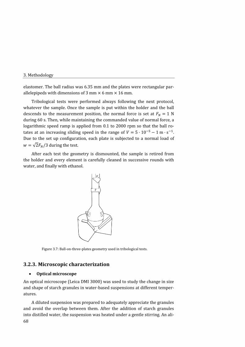
3. Methodology
68
elastomer. The ball radius was 6.35 mm and the plates were rectangular par-
allelepipeds with dimensions of 3 mm × 6 mm × 16 mm.
Tribological tests were performed always following the next protocol,
whatever the sample. Once the sample is put within the holder and the ball
descends to the measurement position, the normal force is set at 𝐹𝑁 = 1 N
during 60 s. Then, while maintaining the commanded value of normal force, a
logarithmic speed ramp is applied from 0.1 to 2000 rpm so that the ball ro-
tates at an increasing sliding speed in the range of 𝑉 = 5 · 10−5 − 1 m · s−1.
Due to the set up configuration, each plate is subjected to a normal load of
𝑤 = √2𝐹𝑁/3 during the test.
After each test the geometry is dismounted, the sample is retired from
the holder and every element is carefully cleaned in successive rounds with
water, and finally with ethanol.
Figure 3.7: Ball-on-three-plates geometry used in tribological tests.
Microscopic characterization 3.2.3.
Optical microscope
An optical microscope (Leica DMI 3000) was used to study the change in size
and shape of starch granules in water-based suspensions at different temper-
atures.
A diluted suspension was prepared to adequately appreciate the granules
and avoid the overlap between them. After the addition of starch granules
into distilled water, the suspension was heated under a gentle stirring. An ali-
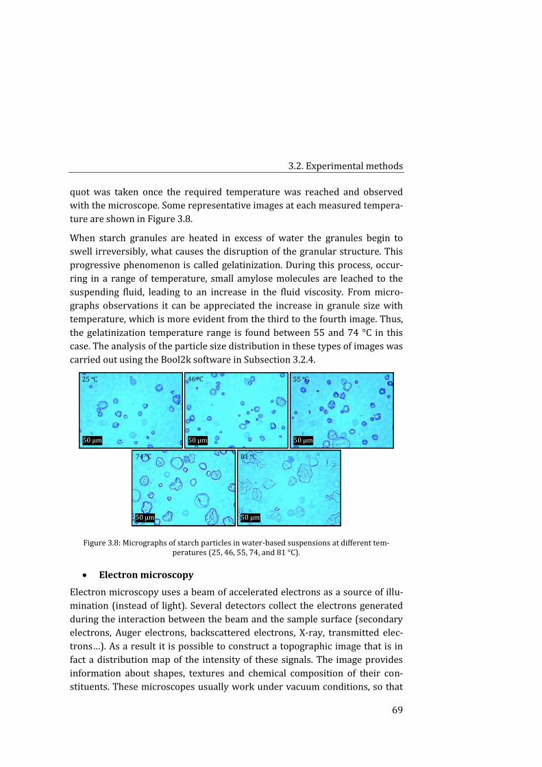
3.2. Experimental methods
69
quot was taken once the required temperature was reached and observed
with the microscope. Some representative images at each measured tempera-
ture are shown in Figure 3.8.
When starch granules are heated in excess of water the granules begin to
swell irreversibly, what causes the disruption of the granular structure. This
progressive phenomenon is called gelatinization. During this process, occur-
ring in a range of temperature, small amylose molecules are leached to the
suspending fluid, leading to an increase in the fluid viscosity. From micro-
graphs observations it can be appreciated the increase in granule size with
temperature, which is more evident from the third to the fourth image. Thus,
the gelatinization temperature range is found between 55 and 74 °C in this
case. The analysis of the particle size distribution in these types of images was
carried out using the Bool2k software in Subsection 3.2.4.
Figure 3.8: Micrographs of starch particles in water-based suspensions at different tem-peratures (25, 46, 55, 74, and 81 °C).
Electron microscopy
Electron microscopy uses a beam of accelerated electrons as a source of illu-
mination (instead of light). Several detectors collect the electrons generated
during the interaction between the beam and the sample surface (secondary
electrons, Auger electrons, backscattered electrons, X-ray, transmitted elec-
trons…). As a result it is possible to construct a topographic image that is in
fact a distribution map of the intensity of these signals. The image provides
information about shapes, textures and chemical composition of their con-
stituents. These microscopes usually work under vacuum conditions, so that
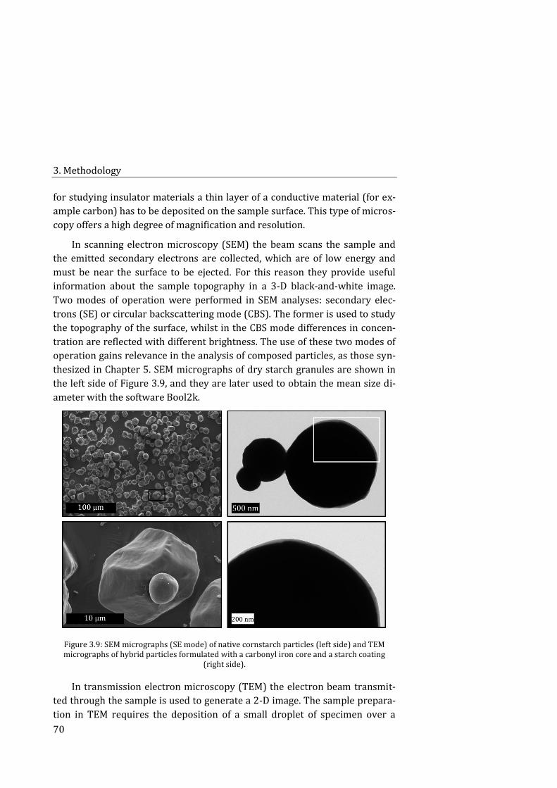
3. Methodology
70
for studying insulator materials a thin layer of a conductive material (for ex-
ample carbon) has to be deposited on the sample surface. This type of micros-
copy offers a high degree of magnification and resolution.
In scanning electron microscopy (SEM) the beam scans the sample and
the emitted secondary electrons are collected, which are of low energy and
must be near the surface to be ejected. For this reason they provide useful
information about the sample topography in a 3-D black-and-white image.
Two modes of operation were performed in SEM analyses: secondary elec-
trons (SE) or circular backscattering mode (CBS). The former is used to study
the topography of the surface, whilst in the CBS mode differences in concen-
tration are reflected with different brightness. The use of these two modes of
operation gains relevance in the analysis of composed particles, as those syn-
thesized in Chapter 5. SEM micrographs of dry starch granules are shown in
the left side of Figure 3.9, and they are later used to obtain the mean size di-
ameter with the software Bool2k.
Figure 3.9: SEM micrographs (SE mode) of native cornstarch particles (left side) and TEM micrographs of hybrid particles formulated with a carbonyl iron core and a starch coating
(right side).
In transmission electron microscopy (TEM) the electron beam transmit-
ted through the sample is used to generate a 2-D image. The sample prepara-
tion in TEM requires the deposition of a small droplet of specimen over a
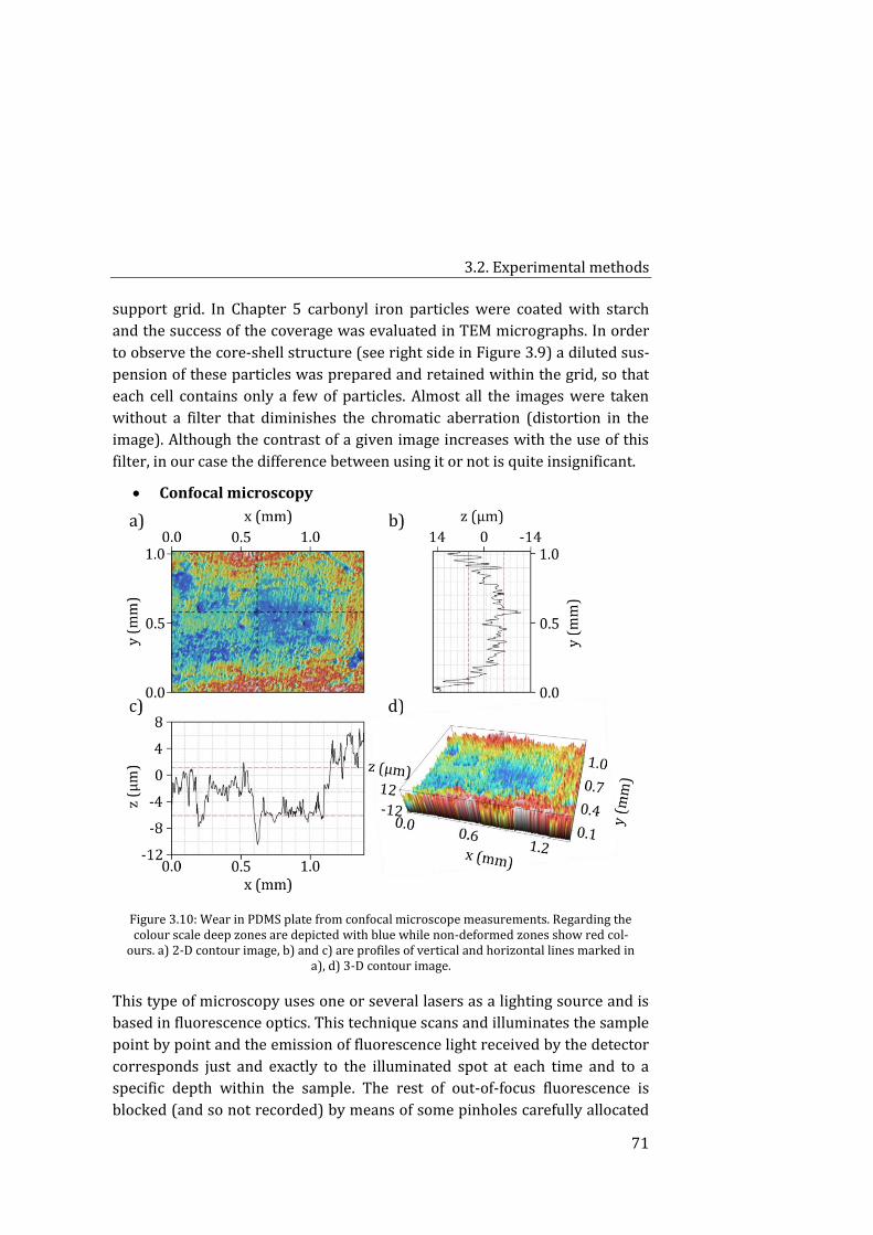
3.2. Experimental methods
71
support grid. In Chapter 5 carbonyl iron particles were coated with starch
and the success of the coverage was evaluated in TEM micrographs. In order
to observe the core-shell structure (see right side in Figure 3.9) a diluted sus-
pension of these particles was prepared and retained within the grid, so that
each cell contains only a few of particles. Almost all the images were taken
without a filter that diminishes the chromatic aberration (distortion in the
image). Although the contrast of a given image increases with the use of this
filter, in our case the difference between using it or not is quite insignificant.
Confocal microscopy
Figure 3.10: Wear in PDMS plate from confocal microscope measurements. Regarding the colour scale deep zones are depicted with blue while non-deformed zones show red col-
ours. a) 2-D contour image, b) and c) are profiles of vertical and horizontal lines marked in a), d) 3-D contour image.
This type of microscopy uses one or several lasers as a lighting source and is
based in fluorescence optics. This technique scans and illuminates the sample
point by point and the emission of fluorescence light received by the detector
corresponds just and exactly to the illuminated spot at each time and to a
specific depth within the sample. The rest of out-of-focus fluorescence is
blocked (and so not recorded) by means of some pinholes carefully allocated
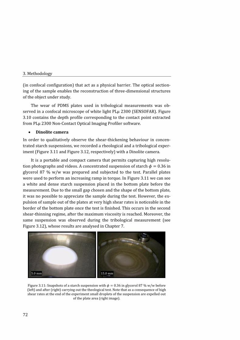
3. Methodology
72
(in confocal configuration) that act as a physical barrier. The optical section-
ing of the sample enables the reconstruction of three-dimensional structures
of the object under study.
The wear of PDMS plates used in tribological measurements was ob-
served in a confocal microscope of white light PLμ 2300 (SENSOFAR). Figure
3.10 contains the depth profile corresponding to the contact point extracted
from PLμ 2300 Non-Contact Optical Imaging Profiler software.
Dinolite camera
In order to qualitatively observe the shear-thickening behaviour in concen-
trated starch suspensions, we recorded a rheological and a tribological exper-
iment (Figure 3.11 and Figure 3.12, respectively) with a Dinolite camera.
It is a portable and compact camera that permits capturing high resolu-
tion photographs and videos. A concentrated suspension of starch 𝜙 = 0.36 in
glycerol 87 % w/w was prepared and subjected to the test. Parallel plates
were used to perform an increasing ramp in torque. In Figure 3.11 we can see
a white and dense starch suspension placed in the bottom plate before the
measurement. Due to the small gap chosen and the shape of the bottom plate,
it was no possible to appreciate the sample during the test. However, the ex-
pulsion of sample out of the plates at very high shear rates is noticeable in the
border of the bottom plate once the test is finished. This occurs in the second
shear-thinning regime, after the maximum viscosity is reached. Moreover, the
same suspension was observed during the tribological measurement (see
Figure 3.12), whose results are analysed in Chapter 7.
Figure 3.11: Snapshots of a starch suspension with 𝜙 = 0.36 in glycerol 87 % w/w before (left) and after (right) carrying out the theological test. Note that as a consequence of high shear rates at the end of the experiment small droplets of the suspension are expelled out
of the plate area (right image).
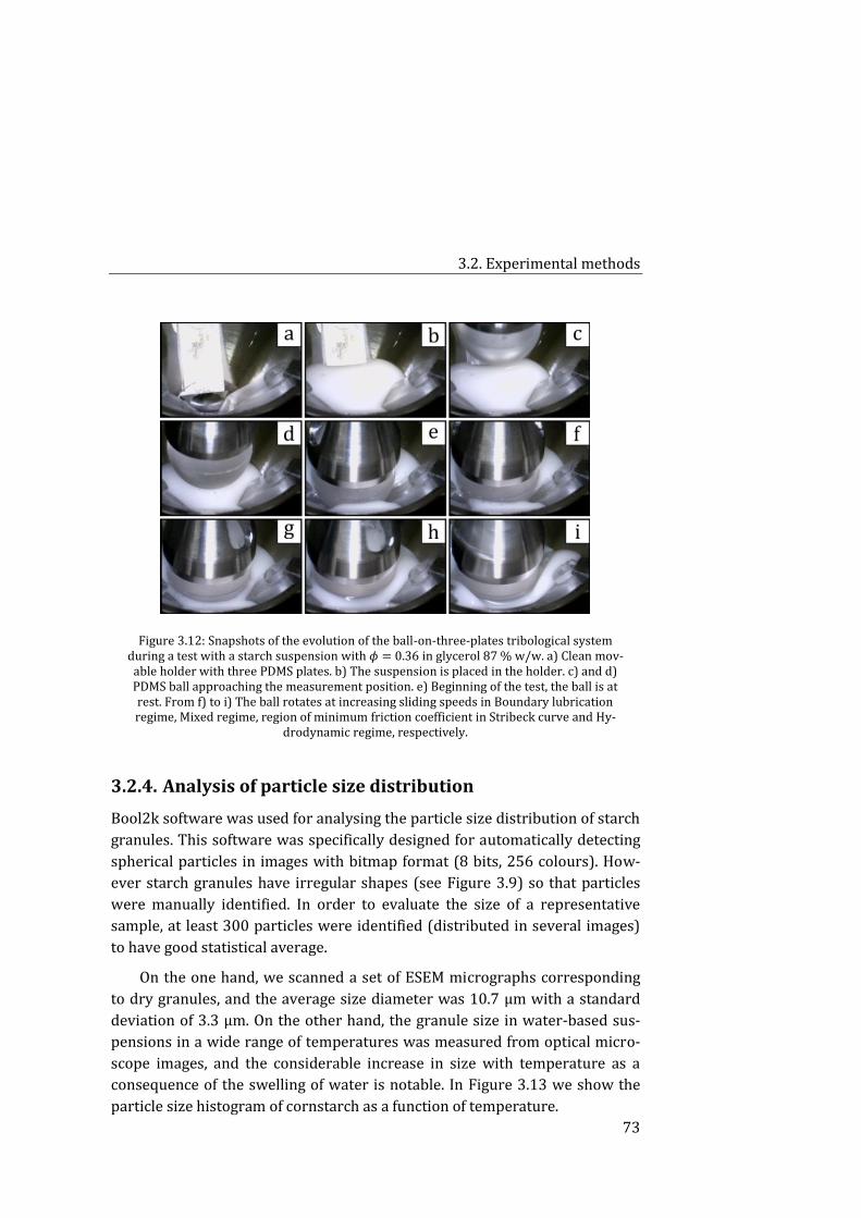
3.2. Experimental methods
73
Figure 3.12: Snapshots of the evolution of the ball-on-three-plates tribological system during a test with a starch suspension with 𝜙 = 0.36 in glycerol 87 % w/w. a) Clean mov-
able holder with three PDMS plates. b) The suspension is placed in the holder. c) and d) PDMS ball approaching the measurement position. e) Beginning of the test, the ball is at rest. From f) to i) The ball rotates at increasing sliding speeds in Boundary lubrication regime, Mixed regime, region of minimum friction coefficient in Stribeck curve and Hy-
drodynamic regime, respectively.
Analysis of particle size distribution 3.2.4.
Bool2k software was used for analysing the particle size distribution of starch
granules. This software was specifically designed for automatically detecting
spherical particles in images with bitmap format (8 bits, 256 colours). How-
ever starch granules have irregular shapes (see Figure 3.9) so that particles
were manually identified. In order to evaluate the size of a representative
sample, at least 300 particles were identified (distributed in several images)
to have good statistical average.
On the one hand, we scanned a set of ESEM micrographs corresponding
to dry granules, and the average size diameter was 10.7 μm with a standard
deviation of 3.3 μm. On the other hand, the granule size in water-based sus-
pensions in a wide range of temperatures was measured from optical micro-
scope images, and the considerable increase in size with temperature as a
consequence of the swelling of water is notable. In Figure 3.13 we show the
particle size histogram of cornstarch as a function of temperature.
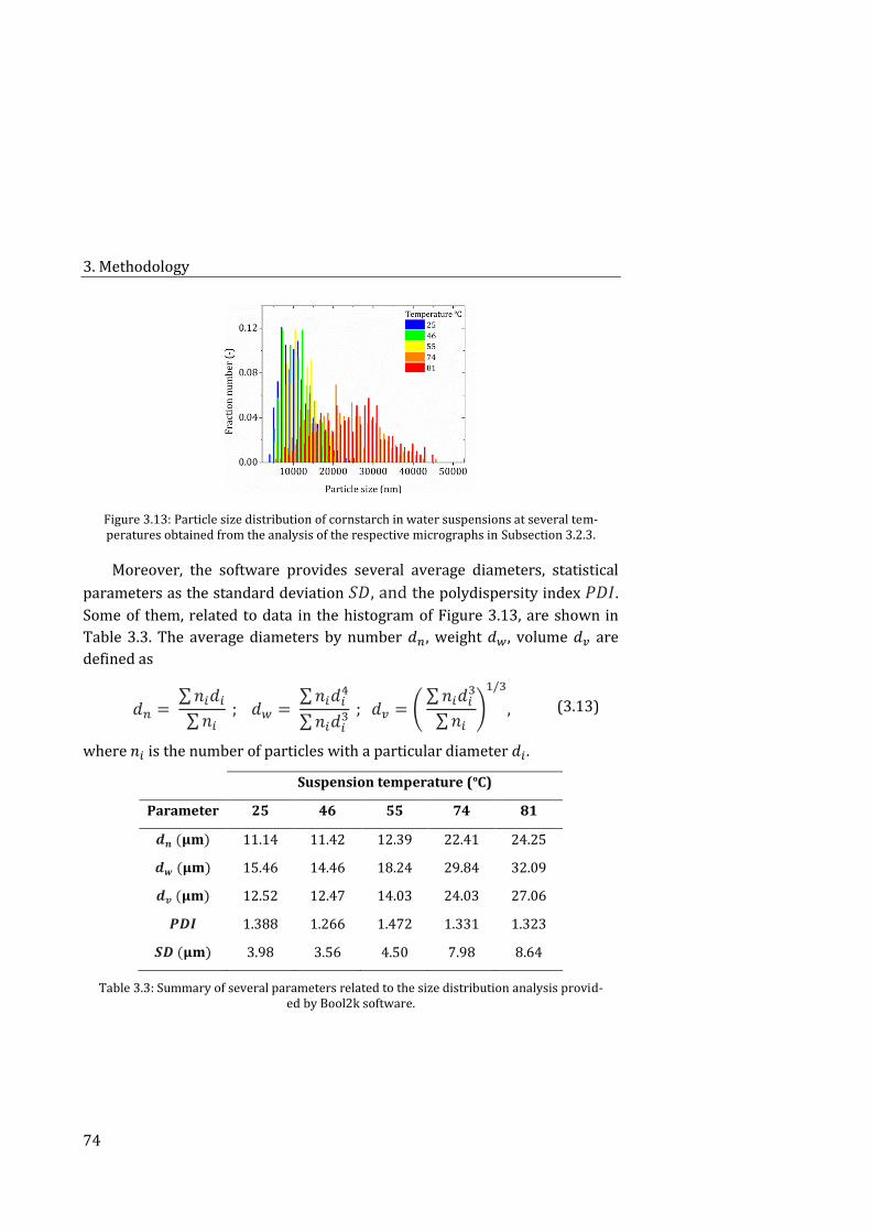
3. Methodology
74
Figure 3.13: Particle size distribution of cornstarch in water suspensions at several tem-peratures obtained from the analysis of the respective micrographs in Subsection 3.2.3.
Moreover, the software provides several average diameters, statistical
parameters as the standard deviation 𝑆𝐷, and the polydispersity index 𝑃𝐷𝐼.
Some of them, related to data in the histogram of Figure 3.13, are shown in
Table 3.3. The average diameters by number 𝑑𝑛, weight 𝑑𝑤, volume 𝑑𝑣 are
defined as
𝑑𝑛 = ∑ 𝑛𝑖𝑑𝑖
∑ 𝑛𝑖 ; 𝑑𝑤 =
∑ 𝑛𝑖𝑑𝑖4
∑ 𝑛𝑖𝑑𝑖3 ; 𝑑𝑣 = (
∑ 𝑛𝑖𝑑𝑖3
∑ 𝑛𝑖)
1/3
, (3.13)
where 𝑛𝑖 is the number of particles with a particular diameter 𝑑𝑖 .
Suspension temperature (ºC)
Parameter 25 46 55 74 81
𝒅𝒏 (𝛍𝐦) 11.14 11.42 12.39 22.41 24.25
𝒅𝒘 (𝛍𝐦) 15.46 14.46 18.24 29.84 32.09
𝒅𝒗 (𝛍𝐦) 12.52 12.47 14.03 24.03 27.06
𝑷𝑫𝑰 1.388 1.266 1.472 1.331 1.323
𝑺𝑫 (𝛍𝐦) 3.98 3.56 4.50 7.98 8.64
Table 3.3: Summary of several parameters related to the size distribution analysis provid-ed by Bool2k software.
3.2. Experimental methods
75
Colloidal stability 3.2.5.
Zetasizer Nano Z
In Chapter 5 we prepared mixed suspensions of starch and carbonyl iron par-
ticles in water. Before the addition of carbonyl iron particles to the shear-
thickening fluid, it is important to determine if both types of particles would
interact due to their charges. For this reason we performed measurements of
electrophoretic mobility of starch and carbonyl iron particles in a Zetasizer
Nano Z device (Malvern Instruments). Size measurements of starch suspen-
sions were also carried out in this apparatus.
This instrument is based on Dynamic Light Scattering (DLS) for size
measurements. The scattering of light produced in all directions when a laser
beam collides with suspended particles fluctuates with time due to the ran-
dom Brownian motion of the particles. In this sense, reliable measurements
depend on the sample concentration; if it is too low the light scattering may
be insufficient, while if the sample is too concentrated multiple scattering
phenomena may be produced and the free diffusion of the particles may com-
plicate. Moreover, it is known that large particles move slowly than small
ones. The Stokes-Einstein equation [47] relates the particle size and its speed,
expressed in terms of the hydrodynamic diameter 𝐷ℎ and the diffusion coeffi-
cient 𝐷, respectively:
𝐷 =𝑘𝐵𝑇
3𝜋휂𝐷ℎ , (3.14)
where 𝑘𝐵 is the Boltzmann’s constant, 𝑇 the absolute temperature and 휂 the
solvent viscosity.
When a charged particle is suspended in a liquid ions with an opposite
charge become attracted to the particle surface forming a region of strongly
bound ions called Stern layer. Then a diffuse layer of ions is distributed
around this inner one. Both layers, Stern and diffuse, define the so-called elec-
trical double layer and the potential existing at the end of the diffuse layer is
called zeta potential 휁. It is worth noting that 휁 cannot be directly measured in
Zetasizer Nano Z system but instead the electrophoretic mobility. When an
electric field 𝐸 is applied to a suspension containing charged particles they
then move with a constant velocity, called electrophoretic velocity 𝑈, towards
the electrode of opposite charge. This velocity is the result of a balance be-
tween the applied electric field and the viscous resistance of the solvent to the

3. Methodology
76
movement of the particles. If 𝐸 is weak enough, 𝑈 = 𝜇𝑒𝐸, being the constant
of proportionality the electrophoretic mobility 𝜇𝑒 . At this time the incident
beams shot the sample and the scattered light undergoes a fluctuating inten-
sity signal that is proportional to the speed of the particles. The calculation of
𝜇𝑒 is carried out by LDV (Laser Doppler Velocimetry) combined with a laser
interferometric technique called M3-PALS (Phase analysis Light Scattering
[48]. The application of Henry equation [49] permits relating the electropho-
retic mobility to the zeta potential through this expression:
𝜇𝑒 =2휀휁𝑓(𝜅𝑎)
3휂 , (3.15)
where 휀 is the dielectric constant of the medium, 𝑓(𝜅𝑎) is the Henry’s func-
tion and depends on the particle shape, 𝜅 is the Debye length (somehow the
inverse of the thickness of the double layer), and 𝑎 is the particle radius.
The main factor influencing zeta potential is pH. The 휁-pH curve of a sys-
tem of charged particles usually moves from positive values at low pH to neg-
ative values at high pH, and the transition point at which 휁 = 0 is called the
isoelectric point. The value of 휁 is related to the system stability; from
휁 ∈ (−30, 30) mV the system is considered as unstable because there is no
force preventing the particle attraction and flocculation, while outside this
interval repulsion exists and there is no tendency to flocculate.
A model sample (AJ13) has to be prepared, inserted in the measuring cell,
and measured in the device in order to evaluate the correct calibration of the
apparatus and the well operation of the cell. After that, regular measurements
can be performed. We used a folded capillary cell (DTS1070) to carry out both
size and electrokinetic measurements. An important aspect to consider
(mainly in electrophoretic measurements) is that the minimum volume of
sample to be introduced in the cell for it to be in contact with the electrodes is
0.75 ml. Ultrasonication is frequently used during the sample preparation to
remove air bubbles or to breakup particle aggregates, which can lead to erro-
neous results. In this sense, a careful filling with a syringe is desirable to avoid
air bubbles in the cell.
In spite of the limitations in size (particle sizes above 6000 nm provide
error messages) we performed size measurements at 25 °C of two diluted
suspensions of starch in water, with volume fractions 𝜙𝑆𝑡𝑎𝑟𝑐ℎ = 0.001 and
0.01. Granule size reported in the former case was 5835 ± 2068 nm, and 4727
± 833 nm for the suspension with 𝜙𝑆𝑡𝑎𝑟𝑐ℎ = 0.01. It is noticeable that in both
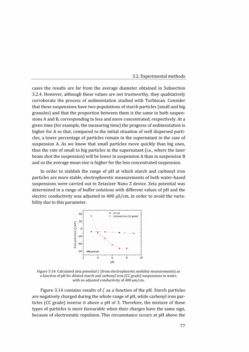
3.2. Experimental methods
77
cases the results are far from the average diameter obtained in Subsection
3.2.4. However, although these values are not trustworthy, they qualitatively
corroborate the process of sedimentation studied with Turbiscan. Consider
that these suspensions have two populations of starch particles (small and big
granules) and that the proportion between them is the same in both suspen-
sions A and B, corresponding to less and more concentrated, respectively. At a
given time (for example, the measuring time) the progress of sedimentation is
higher for A so that, compared to the initial situation of well dispersed parti-
cles, a lower percentage of particles remain in the supernatant in the case of
suspension A. As we know that small particles move quickly than big ones,
thus the rate of small to big particles in the supernatant (i.e., where the laser
beam shot the suspension) will be lower in suspension A than in suspension B
and so the average mean size is higher for the less concentrated suspension.
In order to stablish the range of pH at which starch and carbonyl iron
particles are more stable, electrophoretic measurements of both water-based
suspensions were carried out in Zetasizer Nano Z device. Zeta potential was
determined in a range of buffer solutions with different values of pH and the
electric conductivity was adjusted to 400 μS/cm, in order to avoid the varia-
bility due to this parameter.
Figure 3.14: Calculated zeta potential 휁 (from electrophoretic mobility measurements) as a function of pH for diluted starch and carbonyl iron (CC grade) suspensions in water,
with an adjusted conductivity of 400 μm/cm.
Figure 3.14 contains results of 휁 as a function of the pH. Starch particles
are negatively charged during the whole range of pH, while carbonyl iron par-
ticles (CC grade) inverse it above a pH of 3. Therefore, the mixture of these
types of particles is more favourable when their charges have the same sign,
because of electrostatic repulsion. This circumstance occurs at pH above the
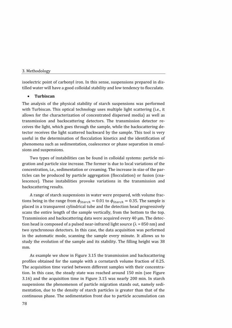
3. Methodology
78
isoelectric point of carbonyl iron. In this sense, suspensions prepared in dis-
tilled water will have a good colloidal stability and low tendency to flocculate.
Turbiscan
The analysis of the physical stability of starch suspensions was performed
with Turbiscan. This optical technology uses multiple light scattering (i.e., it
allows for the characterization of concentrated dispersed media) as well as
transmission and backscattering detectors. The transmission detector re-
ceives the light, which goes through the sample, while the backscattering de-
tector receives the light scattered backward by the sample. This tool is very
useful in the determination of flocculation kinetics and the identification of
phenomena such as sedimentation, coalescence or phase separation in emul-
sions and suspensions.
Two types of instabilities can be found in colloidal systems: particle mi-
gration and particle size increase. The former is due to local variations of the
concentration, i.e., sedimentation or creaming. The increase in size of the par-
ticles can be produced by particle aggregation (flocculation) or fusion (coa-
lescence). These instabilities provoke variations in the transmission and
backscattering results.
A range of starch suspensions in water were prepared, with volume frac-
tions being in the range from 𝜙𝑆𝑡𝑎𝑟𝑐ℎ = 0.01 to 𝜙𝑆𝑡𝑎𝑟𝑐ℎ = 0.35. The sample is
placed in a transparent cylindrical tube and the detection head progressively
scans the entire length of the sample vertically, from the bottom to the top.
Transmission and backscattering data were acquired every 40 μm. The detec-
tion head is composed of a pulsed near-infrared light source ( = 850 nm) and
two synchronous detectors. In this case, the data acquisition was performed
in the automatic mode, scanning the sample every minute. It allows us to
study the evolution of the sample and its stability. The filling height was 38
mm.
As example we show in Figure 3.15 the transmission and backscattering
profiles obtained for the sample with a cornstarch volume fraction of 0.25.
The acquisition time varied between different samples with their concentra-
tion. In this case, the steady state was reached around 150 min (see Figure
3.16) and the acquisition time in Figure 3.15 was nearly 200 min. In starch
suspensions the phenomenon of particle migration stands out, namely sedi-
mentation, due to the density of starch particles is greater than that of the
continuous phase. The sedimentation front due to particle accumulation can
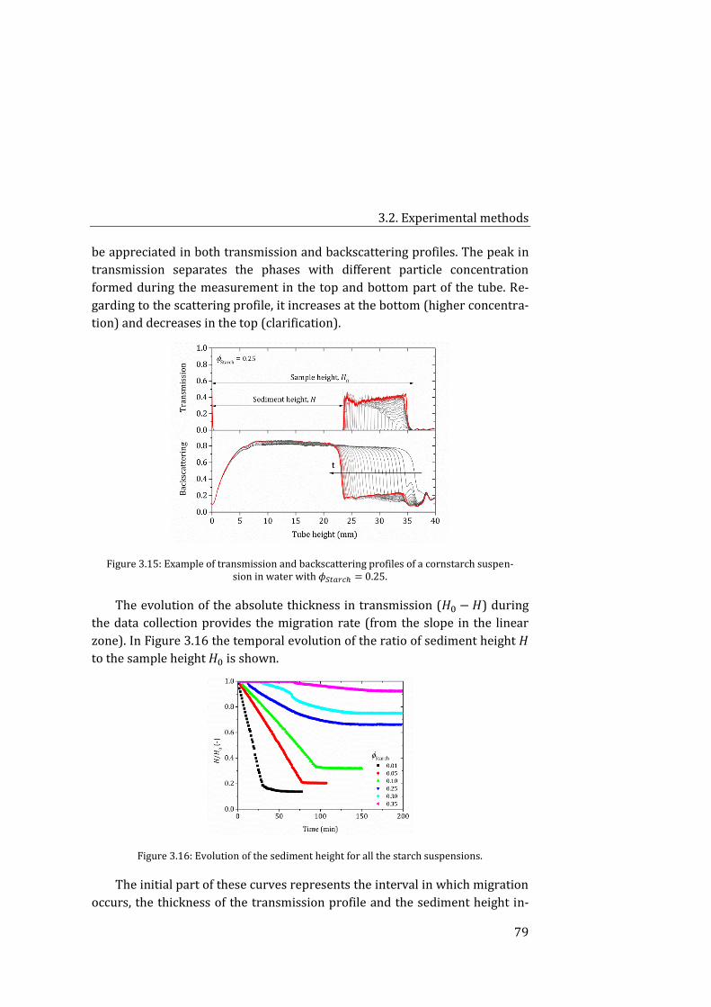
3.2. Experimental methods
79
be appreciated in both transmission and backscattering profiles. The peak in
transmission separates the phases with different particle concentration
formed during the measurement in the top and bottom part of the tube. Re-
garding to the scattering profile, it increases at the bottom (higher concentra-
tion) and decreases in the top (clarification).
Figure 3.15: Example of transmission and backscattering profiles of a cornstarch suspen-sion in water with 𝜙𝑆𝑡𝑎𝑟𝑐ℎ = 0.25.
The evolution of the absolute thickness in transmission (𝐻0 − 𝐻) during
the data collection provides the migration rate (from the slope in the linear
zone). In Figure 3.16 the temporal evolution of the ratio of sediment height 𝐻
to the sample height 𝐻0 is shown.
Figure 3.16: Evolution of the sediment height for all the starch suspensions.
The initial part of these curves represents the interval in which migration
occurs, the thickness of the transmission profile and the sediment height in-
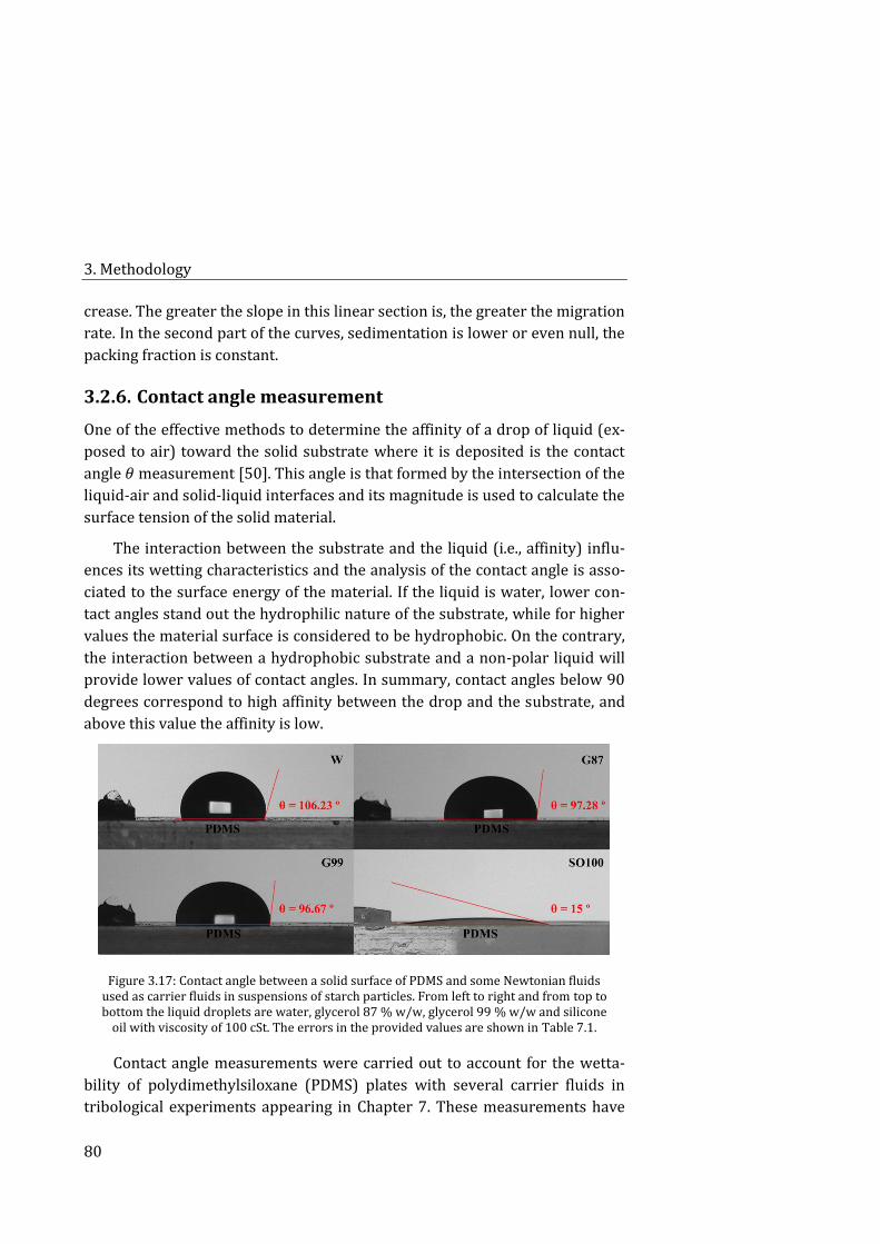
3. Methodology
80
crease. The greater the slope in this linear section is, the greater the migration
rate. In the second part of the curves, sedimentation is lower or even null, the
packing fraction is constant.
Contact angle measurement 3.2.6.
One of the effective methods to determine the affinity of a drop of liquid (ex-
posed to air) toward the solid substrate where it is deposited is the contact
angle 휃 measurement [50]. This angle is that formed by the intersection of the
liquid-air and solid-liquid interfaces and its magnitude is used to calculate the
surface tension of the solid material.
The interaction between the substrate and the liquid (i.e., affinity) influ-
ences its wetting characteristics and the analysis of the contact angle is asso-
ciated to the surface energy of the material. If the liquid is water, lower con-
tact angles stand out the hydrophilic nature of the substrate, while for higher
values the material surface is considered to be hydrophobic. On the contrary,
the interaction between a hydrophobic substrate and a non-polar liquid will
provide lower values of contact angles. In summary, contact angles below 90
degrees correspond to high affinity between the drop and the substrate, and
above this value the affinity is low.
Figure 3.17: Contact angle between a solid surface of PDMS and some Newtonian fluids used as carrier fluids in suspensions of starch particles. From left to right and from top to bottom the liquid droplets are water, glycerol 87 % w/w, glycerol 99 % w/w and silicone
oil with viscosity of 100 cSt. The errors in the provided values are shown in Table 7.1.
Contact angle measurements were carried out to account for the wetta-
bility of polydimethylsiloxane (PDMS) plates with several carrier fluids in
tribological experiments appearing in Chapter 7. These measurements have
3.2. Experimental methods
81
to be carried out under very controlled and clean conditions as contact angle
is extremely sensitive to impurities.
We performed direct measurement of contact angles using the static ses-
sile drop method at 25 °C. A contact angle goniometer is coupled with a cam-
era that captures the profile of a drop placed over the horizontal surface, and
the tangent angle to the drop at the three-phase equilibrium interfacial point
is measured with an own software called Contacto. This method is character-
ized by its simplicity and the small amount of surface area of solid substrates
and liquid volume needed to perform the measurement. The program is ca-
pable of providing information about the surface tension, drop volume and
contact radius.
Figure 3.17 shows the droplet profiles captured during the static sessile
drop method carried out with PDMS substrates and several fluids. The value
of the measured contact angle appears in the images, and the hydrophobicity
of the substrate is confirmed. It is worth noting the low contact angle in the
case of the drop of silicone oil (SO100). This value is an approximation and
was calculated geometrically, as for such low values the software is not able
to measure it accurately. In this case no value was provided by Contacto due
to the uncertainty of locating the tangent line in such a flat drop profile.
Calibration of the magnetic field applied by a solenoid 3.2.7.
In most measurements in squeeze experiments the magnetic field is applied
by the magnetorheological cell. However, in order to determine if a field gra-
dient was affecting the strengthening effect in Subsection 8.5.5. we compared
the results using a solenoid with those carried out within the magnetorheo-
logical cell, both at low magnetic field (15 mT).
The solenoid employed in these measurements had inner and outer radii
of 9 cm and 15.6 cm, respectively, a ring thickness of 3 cm, and the height of
turns was 4.5 cm. The use of this coil allows us to work at low magnetic in-
ductions, from 0 to 20 mT. For the calibration of the solenoid a transverse
probe has to be placed in the last loop of the magnetic coil, so that the meas-
uring part (there is a mark in the correct position) to be in the centre of the
solenoid, where the value of the magnetic field is maximum. First of all, the
probe is introduced in a zero flux chamber. Then, the probe is fixed in the
suitable position and we measure the magnetic induction as the voltage or
intensity is tuned in the power supply.
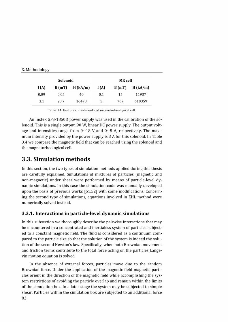
3. Methodology
82
Solenoid MR cell
I (A) B (mT) H (kA/m) I (A) B (mT) H (kA/m)
0.09 0.05 40 0.1 15 11937
3.1 20.7 16473 5 767 610359
Table 3.4: Features of solenoid and magnetorheological cell.
An Instek GPS-1850D power supply was used in the calibration of the so-
lenoid. This is a single output, 90 W, linear DC power supply. The output volt-
age and intensities range from 0~18 V and 0~5 A, respectively. The maxi-
mum intensity provided by the power supply is 3 A for this solenoid. In Table
3.4 we compare the magnetic field that can be reached using the solenoid and
the magnetorheological cell.
Simulation methods 3.3.
In this section, the two types of simulation methods applied during this thesis
are carefully explained. Simulations of mixtures of particles (magnetic and
non-magnetic) under shear were performed by means of particle-level dy-
namic simulations. In this case the simulation code was manually developed
upon the basis of previous works [51,52] with some modifications. Concern-
ing the second type of simulations, equations involved in EHL method were
numerically solved instead.
Interactions in particle-level dynamic simulations 3.3.1.
In this subsection we thoroughly describe the pairwise interactions that may
be encountered in a concentrated and inertialess system of particles subject-
ed to a constant magnetic field. The fluid is considered as a continuum com-
pared to the particle size so that the solution of the system is indeed the solu-
tion of the second Newton’s law. Specifically, when both Brownian movement
and friction terms contribute to the total force acting on the particles Lange-
vin motion equation is solved.
In the absence of external forces, particles move due to the random
Brownian force. Under the application of the magnetic field magnetic parti-
cles orient in the direction of the magnetic field while accomplishing the sys-
tem restrictions of avoiding the particle overlap and remain within the limits
of the simulation box. In a later stage the system may be subjected to simple
shear. Particles within the simulation box are subjected to an additional force
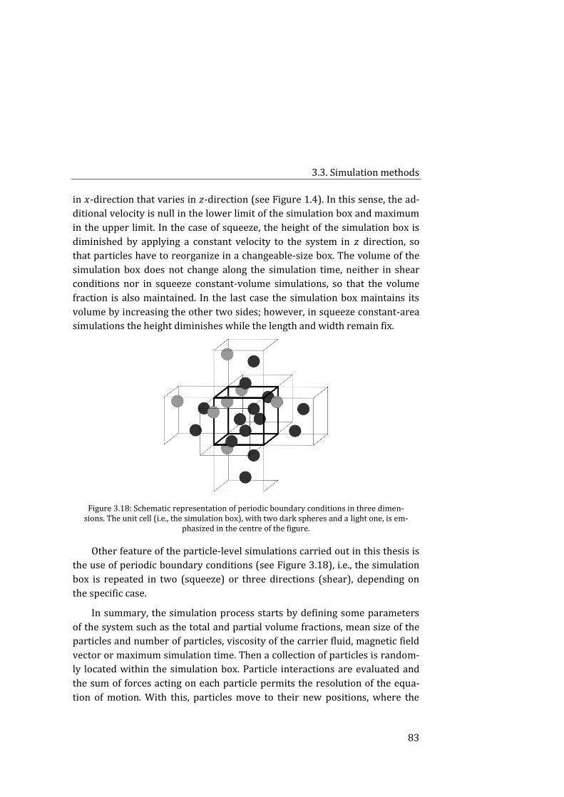
3.3. Simulation methods
83
in 𝑥-direction that varies in 𝑧-direction (see Figure 1.4). In this sense, the ad-
ditional velocity is null in the lower limit of the simulation box and maximum
in the upper limit. In the case of squeeze, the height of the simulation box is
diminished by applying a constant velocity to the system in 𝑧 direction, so
that particles have to reorganize in a changeable-size box. The volume of the
simulation box does not change along the simulation time, neither in shear
conditions nor in squeeze constant-volume simulations, so that the volume
fraction is also maintained. In the last case the simulation box maintains its
volume by increasing the other two sides; however, in squeeze constant-area
simulations the height diminishes while the length and width remain fix.
Figure 3.18: Schematic representation of periodic boundary conditions in three dimen-sions. The unit cell (i.e., the simulation box), with two dark spheres and a light one, is em-
phasized in the centre of the figure.
Other feature of the particle-level simulations carried out in this thesis is
the use of periodic boundary conditions (see Figure 3.18), i.e., the simulation
box is repeated in two (squeeze) or three directions (shear), depending on
the specific case.
In summary, the simulation process starts by defining some parameters
of the system such as the total and partial volume fractions, mean size of the
particles and number of particles, viscosity of the carrier fluid, magnetic field
vector or maximum simulation time. Then a collection of particles is random-
ly located within the simulation box. Particle interactions are evaluated and
the sum of forces acting on each particle permits the resolution of the equa-
tion of motion. With this, particles move to their new positions, where the
3. Methodology
84
forces acting on the system are again evaluated in the new time step. The pro-
cess is iterated up to the energy of the system reaches a steady value.
Equation of motion
The understanding of the interactions occurring between particles in close
proximity is essential in the interpretation of the suspension behaviour. The
equation of motion which better describes the interactions between Browni-
an particles is the Langevin equation. It incorporates the deterministic motion
of the particles and additional stochastic forces:
𝑚𝑖
𝑑2𝒓𝒊
𝑑𝑡2= ∑ 𝑭𝒊
𝒆 + 𝑭𝒊𝒉 + 𝑭𝒊
𝒃 , (3.16)
where 𝑚𝑖 is the mass of the particle and 𝒓𝒊 the vector from the origin of coor-
dinates to the position of the particle. 𝑭𝒊𝒆 accounts for interparticle and exter-
nal forces, namely three contributions are considered: magnetic force be-
tween magnetic particles 𝑭𝒊𝒋𝒎, Hertzian repulsive force 𝑭𝒊𝒋
𝒓 and an exponential
wall normal force 𝑭𝒊𝒘 that prevent particle overlap and particle motion be-
yond the walls, respectively. A cut-off radius is had into account to calculate
𝑭𝒊𝒋𝒎 and 𝑭𝒊
𝒘 in order to only consider interactions from particles that really
contribute to the motion of a given particle 𝑖. In the case of the repulsive
force, it is only activated when the particle overlap occurs. Hydrodynamic in-
teractions 𝑭𝒉 comprise the drag force 𝑭𝒊𝑺, consequence of the relative motion
of the particles in the surrounding fluid and approximated by the Stokes’ law,
and lubrication forces 𝑭𝒊𝒍. The pairwise hydrodynamic lubrication interactions
arise between two particles in close contact separated by a small film of fluid,
such as it is found in concentrated suspensions, and can be calculated from
resistance matrices. The random motion of particles within the fluid due to
thermal fluctuations is considered in Brownian force 𝑭𝒃.
If inertia is neglected, Equation 3.16 can be written as
𝜉𝑖
𝑑𝒓𝒊
𝑑𝑡= 𝜉𝑖𝒖𝒊
∞ + 𝑭𝒊𝒍 + 𝑭𝒊
𝒎 + 𝑭𝒊𝒓 + 𝑭𝒊
𝒘 + 𝑭𝒃 , (3.17)
where 𝜉𝑖 = 3𝜋휂𝜎𝑖 is the friction coefficient of particle 𝑖, 휂 is the fluid viscosity
and 𝜎𝑖 is the particle diameter. In order to solve Equation 3.17 it is convenient
to make it dimensionless by means of scaling parameters in Table 3.5:
𝜎𝑖∗ 𝑑𝒓𝒊
∗
𝑑𝑡∗= 𝜎𝑖
∗𝒖𝒊∞∗
+ 𝑭𝒊𝒍∗ + 𝑭𝒊
𝒎∗ + 𝑭𝒊𝒓∗ + 𝑭𝒊
𝒘∗ + 𝑭𝒃∗ . (3.18)
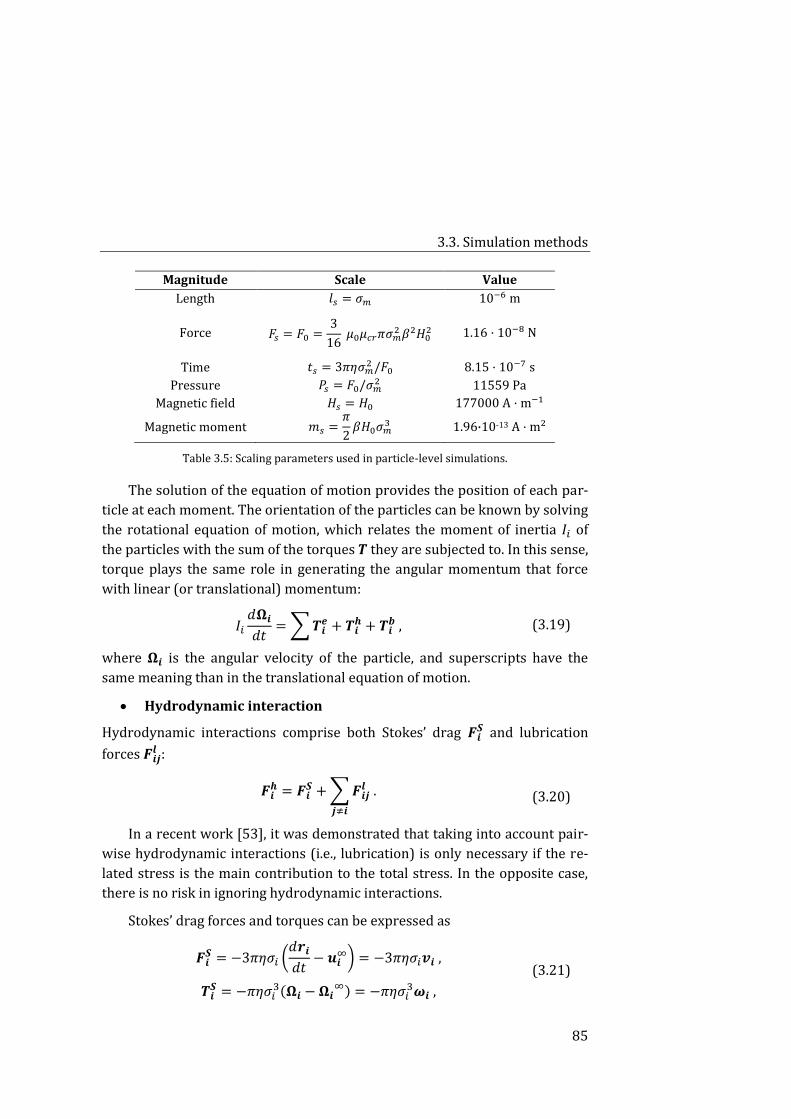
3.3. Simulation methods
85
Magnitude Scale Value
Length 𝑙𝑠 = 𝜎𝑚 10−6 m
Force 𝐹𝑠 = 𝐹0 =3
16 𝜇0𝜇𝑐𝑟𝜋𝜎𝑚
2 𝛽2𝐻02 1.16 · 10−8 N
Time 𝑡𝑠 = 3𝜋휂𝜎𝑚2 /𝐹0 8.15 · 10−7 s
Pressure 𝑃𝑠 = 𝐹0/𝜎𝑚2 11559 Pa
Magnetic field 𝐻𝑠 = 𝐻0 177000 A · m−1
Magnetic moment 𝑚𝑠 =𝜋
2𝛽𝐻0𝜎𝑚
3 1.96·10-13 A · m2
Table 3.5: Scaling parameters used in particle-level simulations.
The solution of the equation of motion provides the position of each par-
ticle at each moment. The orientation of the particles can be known by solving
the rotational equation of motion, which relates the moment of inertia 𝐼𝑖 of
the particles with the sum of the torques 𝑻 they are subjected to. In this sense,
torque plays the same role in generating the angular momentum that force
with linear (or translational) momentum:
𝐼𝑖
𝑑𝛀𝒊
𝑑𝑡= ∑ 𝑻𝒊
𝒆 + 𝑻𝒊𝒉 + 𝑻𝒊
𝒃 , (3.19)
where 𝛀𝒊 is the angular velocity of the particle, and superscripts have the
same meaning than in the translational equation of motion.
Hydrodynamic interaction
Hydrodynamic interactions comprise both Stokes’ drag 𝑭𝒊𝑺 and lubrication
forces 𝑭𝒊𝒋𝒍 :
𝑭𝒊𝒉 = 𝑭𝒊
𝑺 + ∑ 𝑭𝒊𝒋𝒍
𝒋≠𝒊
. (3.20)
In a recent work [53], it was demonstrated that taking into account pair-
wise hydrodynamic interactions (i.e., lubrication) is only necessary if the re-
lated stress is the main contribution to the total stress. In the opposite case,
there is no risk in ignoring hydrodynamic interactions.
Stokes’ drag forces and torques can be expressed as
𝑭𝒊𝑺 = −3𝜋휂𝜎𝑖 (
𝑑𝒓𝒊
𝑑𝑡− 𝒖𝒊
∞) = −3𝜋휂𝜎𝑖𝒗𝒊 ,
𝑻𝒊𝑺 = −𝜋휂𝜎𝑖
3(𝛀𝒊 − 𝛀𝒊∞) = −𝜋휂𝜎𝑖
3𝝎𝒊 ,
(3.21)
3. Methodology
86
with 𝑑𝒓𝒊
𝑑𝑡 being the velocity of the particle, 𝒖𝒊
∞ the velocity of the carrier fluid
at the centre of the particle 𝑖 in the absence of particles, and 𝒗𝒊 is the vector of
the difference. Analogously, 𝝎𝒊 is the difference between the angular velocity
of the particle 𝛀𝒊 and the vorticity of the fluid in the position of the particle
𝛀𝒊∞.
The description of the lubrication forces between two bodies is thorough-
ly explained by Kim and Karrila [55]. Lubrication forces are expressed as a
linear combination of translational motion, rotational motion and shearing
flow (first, second and third term, respectively), each contribution multiplied
by its related resistance matrix:
(𝑭𝒊𝒋
𝒍
𝑭𝒋𝒊𝒍
) = −휂 (𝑨𝒊𝒊 𝑨𝒊𝒋
𝑨𝒋𝒊 𝑨𝒋𝒋) (
𝒗𝒊
𝒗𝒋) − 휂 (
�̃�𝒊𝒊 �̃�𝒊𝒋
�̃�𝒋𝒊 �̃�𝒋𝒋
) (𝝎𝒊
𝝎𝒋)
+ 휂 (�̃�𝒊𝒊 �̃�𝒊𝒋
�̃�𝒋𝒊 �̃�𝒋𝒋
) : (𝑬∞
𝑬∞) .
(3.22)
In the last expression 𝑬∞ is the rate-of strain tensor, and the components
𝐴 and �̃� of the resistance matrices are tensors of rank 2, while �̃� has rank 3.
For the case of particles with axisymmetric geometry, as spheres, the compo-
nents of these tensors are defined [55] as
𝐴𝛼𝛽𝑖𝑗
= 𝑋𝑖𝑗𝐴�̂�𝛼�̂�𝛽 + 𝑌𝑖𝑗
𝐴(𝛿𝛼𝛽 − �̂�𝛼�̂�𝛽) ,
𝐵𝛼𝛽𝑖𝑗
= −𝑌𝑖𝑗𝐵휀𝛼𝛽𝛾�̂�𝛾 ,
𝐺𝛼𝛽𝛾𝑖𝑗
= −𝑋𝑖𝑗𝐺 (�̂�𝛼�̂�𝛽 −
1
3𝛿𝛼𝛽) �̂�𝛾 − 𝑌𝑖𝑗
𝐺(�̂�𝛼𝛿𝛽𝛾 + �̂�𝛽𝛿𝛼𝛾 − 2�̂�𝛼�̂�𝛽�̂�𝛾) .
(3.23)
It is worth noting that indices 𝑖 and 𝑗 refer to particles, while 𝛼, 𝛽 and 𝛾
refer to the component of the tensors. The unitary vector of the relative posi-
tion of particle 𝑖 with respect to particle 𝑗 is �̂� =𝒓𝒊−𝒓𝒋
|𝒓𝒊−𝒓𝒋|=
𝒓𝒊𝒋
|𝒓𝒊𝒋|. Besides, the el-
ements of the resistance matrix obey the following symmetric relationships:
𝐴𝛼𝛽𝑖𝑗
= 𝐴𝛽𝛼𝑗𝑖
, 𝐵𝛼𝛽𝑖𝑗
= �̃�𝛽𝛼𝑗𝑖
, and 𝐺𝛼𝛽𝛾𝑖𝑗
= �̃�𝛾𝛼𝛽𝑗𝑖
. The near field forms of the re-
sistance functions for translation, rotation and shear are expressed as
Translation:
𝑋𝑖𝑖𝐴 = 12𝜋𝑎𝑖
𝜆2
(1 + 𝜆)3
1
휀 , 𝑋𝑗𝑗
𝐴 = 𝑋𝑖𝑖𝐴(𝜆−1) ,
(3.24)

3.3. Simulation methods
87
𝑋𝑖𝑗𝐴 = −12𝜋𝑎𝑖
𝜆2
(1 + 𝜆)3
1
휀 , 𝑋𝑗𝑖
𝐴 = 𝑋𝑖𝑗𝐴(𝜆−1) ,
𝑌𝑖𝑖𝐴 =
8
5𝜋𝑎𝑖
𝜆(2 + 𝜆 + 2𝜆2)
(1 + 𝜆)3ln
1
휀 , 𝑌𝑗𝑗
𝐴 = 𝑌𝑖𝑖𝐴(𝜆−1) ,
𝑌𝑖𝑗𝐴 = −
8
5𝜋𝑎𝑖
𝜆(2 + 𝜆 + 2𝜆2)
(1 + 𝜆)3ln
1
휀 , 𝑌𝑗𝑖
𝐴 = 𝑌𝑖𝑗𝐴(𝜆−1) ;
(3.25)
Rotation:
𝑌𝑖𝑖𝐵 = −
4
5𝜋𝑎𝑖
2 𝜆(4 + 𝜆)
(1 + 𝜆)2ln
1
휀 , 𝑌𝑗𝑗
𝐵 = −𝑌𝑖𝑖𝐵(𝜆−1) ,
𝑌𝑖𝑗𝐵 =
4
5𝜋𝑎𝑖
2 𝜆(4 + 𝜆)
(1 + 𝜆)2ln
1
휀 , 𝑌𝑗𝑖
𝐵 = −𝑌𝑖𝑗𝐵(𝜆−1) ;
(3.26)
Shear:
𝑋𝑖𝑖𝐺 = 12𝜋𝑎𝑖
2 𝜆2
(1 + 𝜆)3
1
휀 , 𝑋𝑗𝑗
𝐺 = −𝑋𝑖𝑖𝐺(𝜆−1) ,
𝑋𝑖𝑗𝐺 = −12𝜋𝑎𝑖
2 𝜆2
(1 + 𝜆)3
1
휀 , 𝑋𝑗𝑖
𝐺 = −𝑋𝑖𝑗𝐺(𝜆−1) ,
𝑌𝑖𝑖𝐺 =
2
5𝜋𝑎𝑖
2 𝜆(4 − 𝜆 + 7𝜆2)
(1 + 𝜆)3ln
1
휀 , 𝑌𝑗𝑗
𝐺 = −𝑌𝑖𝑖𝐺(𝜆−1) ,
𝑌𝑖𝑗𝐺 = −
2
5𝜋𝑎𝑖
2 𝜆(4 − 𝜆 + 7𝜆2)
(1 + 𝜆)3ln
1
휀 , 𝑌𝑗𝑖
𝐺 = −𝑌𝑖𝑗𝐺(𝜆−1) .
(3.27)
The distance between the surfaces of two interacting particles is given by
a normalized parameter 휀 =|𝒓𝒊𝒋|−𝑎𝑖−𝑎𝑗
(𝑎𝑖−𝑎𝑗)/2, 𝑎𝑖 and 𝑎𝑗 accounts for the particle ra-
dius, and 𝜆 = 𝜎𝑗/𝜎𝑖 is the ratio between diameters of the involved particles.
Note that only the leading terms in previous expressions were considered
(i.e., 휀−1 and ln 휀−1), as in the case of concentrated suspensions 휀 will be very
small.
From now on the lubrication force 𝑭𝒊𝒋𝒍 acting on particle 𝑖 due to particle 𝑗
is exposed, after combining Equations from 3.22 to 3.26. Translational 𝑭𝒊𝒋𝒍,𝒕,
rotational 𝑭𝒊𝒋𝒍,𝒓 and shear 𝑭𝒊𝒋
𝒍,𝒔 terms are separately described below:
𝑭𝒊𝒋𝒍,𝒕 = −휂𝑋𝑖𝑖
𝐴𝒗𝒊⊥ − 휂𝑋𝑖𝑗𝐴𝒗𝒋⊥ − 휂𝑌𝑖𝑖
𝐴𝒗𝒊∥ − 휂𝑌𝑖𝑗𝐴𝒗𝒋∥ = (3.28)
3. Methodology
88
= 6𝜋휂𝜎𝑖
𝜆2
(1 + 𝜆)3
1
휀(𝒗𝒋⊥ − 𝒗𝒊⊥) +
+4
5𝜋휂𝜎𝑖
𝜆(2 + 𝜆 + 2𝜆2)
(1 + 𝜆)3ln
1
휀(𝒗𝒋∥ − 𝒗𝒊∥) ;
𝑭𝒊𝒋𝒍,𝒓 = −휂𝑌𝑖𝑖
𝐵(𝝎𝒊 ∧ �̂�) − 휂𝑌𝑗𝑖𝐵(𝝎𝒋 ∧ �̂�) =
=𝜋
5휂𝜎𝑖
2 𝜆(4 + 𝜆)
(1 + 𝜆)2ln
1
휀(𝝎𝒊 ∧ �̂�) +
𝜋
5휂𝜎𝑖
2 𝜆2(4 + 𝜆)
(1 + 𝜆)2ln
1
휀(𝝎𝒋 ∧ �̂�) ;
𝑭𝒊𝒋𝒍,𝒔 = −휂�̇�(𝑋𝑖𝑖
𝐺 + 𝑋𝑗𝑖𝐺)𝑬𝟏 − 휂�̇�(𝑌𝑖𝑖
𝐺 + 𝑌𝑗𝑖𝐺)𝑬𝟐 =
= −3𝜋휂𝜎𝑖2�̇�
𝜆2
(1 + 𝜆)2
1
휀𝑬𝟏 −
𝜋
5휂𝜎𝑖
2�̇�𝜆(2 + 𝜆 + 2𝜆2)
(1 + 𝜆)2ln
1
휀𝑬𝟐 ;
where 𝑬𝟏 =𝟏
�̇�(�̂��̂�: 𝑬∞)�̂� =
𝒙𝒊𝒋𝒛𝒊𝒋
𝒓𝒊𝒋𝟐 �̂� , and 𝑬𝟐 =
𝟐
�̇�(𝑬∞ · �̂� − (�̂��̂�: 𝑬∞)�̂�).
These equations can be normalized by considering the scales of Table 3.5:
𝑭𝒊𝒋𝒍,𝒕∗ = −2𝜎𝑖
∗ 𝜆2
(1 + 𝜆)3
1
휀𝒗𝒊𝒋⊥
∗ −4
15𝜎𝑖
∗ 𝜆(2 + 𝜆 + 2𝜆2)
(1 + 𝜆)3ln
1
휀𝒗𝒊𝒋∥
∗ ;
𝑭𝒊𝒋𝒍,𝒓∗ =
𝜎𝑖∗2
15
𝜆(4 + 𝜆)
(1 + 𝜆)2ln
1
휀(𝝎𝒊
∗ ∧ �̂�) +
+𝜎𝑖
∗2
15
𝜆2(4 + 𝜆)
(1 + 𝜆)2ln
1
휀(𝝎𝒋
∗ ∧ �̂�) ;
𝑭𝒊𝒋𝒍,𝒔∗ = −𝜎𝑖
∗2�̇�∗𝜆2
(1 + 𝜆)2
1
휀𝑬𝟏 −
𝜎𝑖∗2
15�̇�∗
𝜆(2 + 𝜆 + 2𝜆2)
(1 + 𝜆)2ln
1
휀𝑬𝟐 ;
𝑭𝒊𝒋𝒍∗ = 𝑭𝒊𝒋
𝒍,𝒕∗ + 𝑭𝒊𝒋𝒍,𝒓∗ + 𝑭𝒊𝒋
𝒍,𝒔∗ ,
(3.29)
where 𝒗𝒊𝒋⊥ = 𝒗𝒊⊥ − 𝒗𝒋⊥.
It can be demonstrated that the lubrication force on particle 𝑗 due to par-
ticle 𝑖 is 𝑭𝒋𝒊𝒍∗ = −𝑭𝒊𝒋
𝒍∗, and that lubrication forces diverge for particles in con-
tact, i.e., for 휀 = 0.
Similarly to the development of the lubrication force, the torque on parti-
cles of the system can be obtained from the linear combination of analogous
resistance matrices. After some algebra and using 𝐹0𝜎𝑚 as the torque scale,
the total torque that particle 𝑗 exerts to the particle 𝑖, and vice versa are, is
given by:
3.3. Simulation methods
89
𝑻𝒊𝒋𝒍∗ =
𝜎𝑖∗
15
𝜆(4 + 𝜆)
1 + 𝜆[
1
1 + 𝜆�̂� ∧ 𝒗𝒊𝒋
∗ −2𝜎𝑖
∗
4 + 𝜆𝝎𝒊∥
∗ −𝜆𝜎𝑖
∗
2(4 + 𝜆)𝝎𝒋∥
∗ +
+𝜎𝑖
∗�̇�∗
4(2�̂� ∧ 𝑬𝟐)] ln
1
휀 ;
𝑻𝒋𝒊𝒍∗ =
𝜎𝑖∗
15
𝜆2(4 + 𝜆)
1 + 𝜆[
1
1 + 𝜆�̂� ∧ 𝒗𝒊𝒋
∗ −𝜎𝑖
∗
2(4𝜆 + 1)𝝎𝒊∥
∗ −
−2𝜆𝜎𝑖
∗
4𝜆 + 1𝝎𝒋∥
∗ +𝜎𝑖
∗�̇�∗
4(2�̂� ∧ 𝑬𝟐)] ln
1
휀 .
(3.30)
Now we focus on the translational equation of motion for the case of two
particles and resolve the values of velocities of each particle. The interaction
force 𝑭𝒊𝒏𝒕, due to the sum of magnetic, repulsive, wall and Brownian forces, is
balanced to the negative sum of hydrodynamic forces:
𝑭𝟏𝟐𝒊𝒏𝒕 = 3𝜋휂𝜎1𝒗𝟏 + 휂𝑋11
𝐴 (𝒗𝟏⊥ − 𝒗𝟐⊥) + 휂𝑌11𝐴 (𝒗𝟏∥ − 𝒗𝟐∥) ,
𝑭𝟐𝟏𝒊𝒏𝒕 = 3𝜋휂𝜎2𝒗𝟐 + 휂𝑋22
𝐴 (𝒗𝟐⊥ − 𝒗𝟏⊥) + 휂𝑌22𝐴 (𝒗𝟐∥ − 𝒗𝟏∥) ,
𝑭𝟐𝟏𝒊𝒏𝒕 = −𝑭𝟏𝟐
𝒊𝒏𝒕 .
(3.31)
The normal and tangential parts of these forces, divided by 3𝜋휂𝜎1, are
given by:
𝑭𝟏𝟐𝒉⊥̅̅ ̅̅ ̅ = 𝒗𝟏⊥(1 + 𝑋11
𝐴̅̅ ̅̅̅) − 𝒗𝟐⊥𝑋11𝐴̅̅ ̅̅̅ ,
−𝑭𝟏𝟐𝒉⊥̅̅ ̅̅ ̅ = −𝒗𝟏⊥𝑋22
𝐴̅̅ ̅̅ ̅ + 𝒗𝟐⊥(𝜆 + 𝑋22𝐴̅̅ ̅̅ ̅) ,
𝑭𝟏𝟐𝒉∥̅̅ ̅̅ ̅ = 𝒗𝟏∥(1 + 𝑌11
𝐴̅̅ ̅̅ ) − 𝒗𝟐∥𝑌11𝐴̅̅ ̅̅ ,
−𝑭𝟏𝟐𝒉∥̅̅ ̅̅ ̅ = 𝒗𝟏∥𝑌22
𝐴̅̅ ̅̅ − 𝒗𝟐∥(𝜆 + 𝑌22𝐴̅̅ ̅̅ ) ,
(3.32)
where the dimensionless parameters �̅�and �̅� are defined as �̅� = 𝑋/3𝜋𝜎1 and
likewise �̅� = 𝑌/3𝜋𝜎1. This system of four equations with four unknowns can
be straightforward solved as
𝒗𝟏⊥ =𝜆𝑭𝟏𝟐
𝒉⊥̅̅ ̅̅ ̅
𝜆 + 𝑋11𝐴̅̅ ̅̅̅(𝜆 + 1)
, 𝒗𝟐⊥ = −𝑭𝟏𝟐
𝒉⊥̅̅ ̅̅ ̅
𝜆 + 𝑋11𝐴̅̅ ̅̅̅(𝜆 + 1)
,
𝒗𝟏∥ =𝜆𝑭𝟏𝟐
𝒉∥̅̅ ̅̅ ̅
𝜆 + 𝑌11𝐴̅̅ ̅̅ (𝜆 + 1)
, 𝒗𝟐∥ =𝑭𝟏𝟐
𝒉∥̅̅ ̅̅ ̅
𝜆 + 𝑌11𝐴̅̅ ̅̅ (𝜆 + 1)
.
(3.33)
Similarly, the particle velocities can be solved for systems with more than
two particles. In this case the particle velocity is the sum of the velocity of the
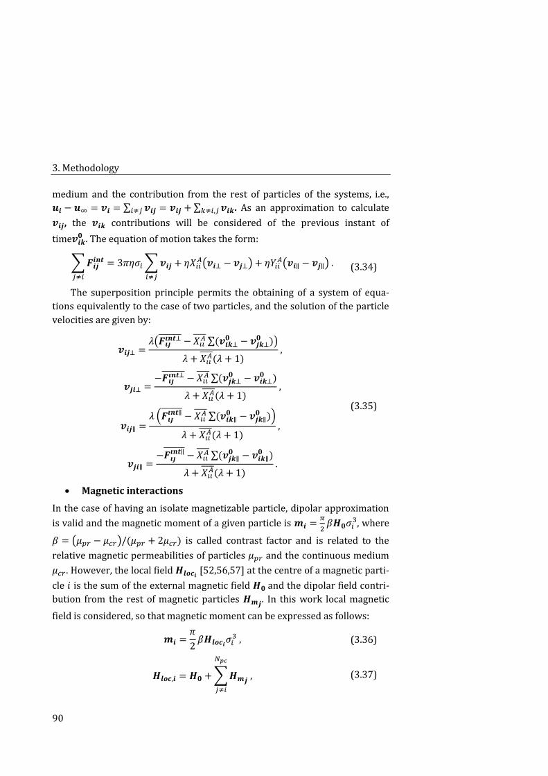
3. Methodology
90
medium and the contribution from the rest of particles of the systems, i.e.,
𝒖𝒊 − 𝒖∞ = 𝒗𝒊 = ∑ 𝒗𝒊𝒋𝑖≠𝑗 = 𝒗𝒊𝒋 + ∑ 𝒗𝒊𝒌𝑘≠𝑖,𝑗 . As an approximation to calculate
𝒗𝒊𝒋, the 𝒗𝒊𝒌 contributions will be considered of the previous instant of
time𝒗𝒊𝒌𝟎 . The equation of motion takes the form:
∑ 𝑭𝒊𝒋𝒊𝒏𝒕
𝑗≠𝑖
= 3𝜋휂𝜎𝑖 ∑ 𝒗𝒊𝒋
𝑖≠𝑗
+ 휂𝑋𝑖𝑖𝐴(𝒗𝒊⊥ − 𝒗𝒋⊥) + 휂𝑌𝑖𝑖
𝐴(𝒗𝒊∥ − 𝒗𝒋∥) . (3.34)
The superposition principle permits the obtaining of a system of equa-
tions equivalently to the case of two particles, and the solution of the particle
velocities are given by:
𝒗𝒊𝒋⊥ =𝜆(𝑭𝒊𝒋
𝒊𝒏𝒕⊥̅̅ ̅̅ ̅̅ ̅ − 𝑋𝑖𝑖𝐴̅̅ ̅̅ ∑(𝒗𝒊𝒌⊥
𝟎 − 𝒗𝒋𝒌⊥𝟎 ))
𝜆 + 𝑋𝑖𝑖𝐴̅̅ ̅̅ (𝜆 + 1)
,
𝒗𝒋𝒊⊥ =−𝑭𝒊𝒋
𝒊𝒏𝒕⊥̅̅ ̅̅ ̅̅ ̅ − 𝑋𝑖𝑖𝐴̅̅ ̅̅ ∑(𝒗𝒋𝒌⊥
𝟎 − 𝒗𝒊𝒌⊥𝟎 )
𝜆 + 𝑋𝑖𝑖𝐴̅̅ ̅̅ (𝜆 + 1)
,
𝒗𝒊𝒋∥ =𝜆 (𝑭𝒊𝒋
𝒊𝒏𝒕∥̅̅ ̅̅ ̅̅ − 𝑋𝑖𝑖𝐴̅̅ ̅̅ ∑(𝒗𝒊𝒌∥
𝟎 − 𝒗𝒋𝒌∥𝟎 ))
𝜆 + 𝑋𝑖𝑖𝐴̅̅ ̅̅ (𝜆 + 1)
,
𝒗𝒋𝒊∥ =−𝑭𝒊𝒋
𝒊𝒏𝒕∥̅̅ ̅̅ ̅̅ − 𝑋𝑖𝑖𝐴̅̅ ̅̅ ∑(𝒗𝒋𝒌∥
𝟎 − 𝒗𝒊𝒌∥𝟎 )
𝜆 + 𝑋𝑖𝑖𝐴̅̅ ̅̅ (𝜆 + 1)
.
(3.35)
Magnetic interactions
In the case of having an isolate magnetizable particle, dipolar approximation
is valid and the magnetic moment of a given particle is 𝒎𝒊 =𝜋
2𝛽𝑯𝟎𝜎𝑖
3, where
𝛽 = (𝜇𝑝𝑟 − 𝜇𝑐𝑟)/(𝜇𝑝𝑟 + 2𝜇𝑐𝑟) is called contrast factor and is related to the
relative magnetic permeabilities of particles 𝜇𝑝𝑟 and the continuous medium
𝜇𝑐𝑟. However, the local field 𝑯𝒍𝒐𝒄𝒊 [52,56,57] at the centre of a magnetic parti-
cle 𝑖 is the sum of the external magnetic field 𝑯𝟎 and the dipolar field contri-
bution from the rest of magnetic particles 𝑯𝒎𝒋. In this work local magnetic
field is considered, so that magnetic moment can be expressed as follows:
𝒎𝒊 =𝜋
2𝛽𝑯𝒍𝒐𝒄𝒊
𝜎𝑖3 , (3.36)
𝑯𝒍𝒐𝒄,𝒊 = 𝑯𝟎 + ∑ 𝑯𝒎𝒋
𝑁𝑝𝑐
𝑗≠𝑖
, (3.37)
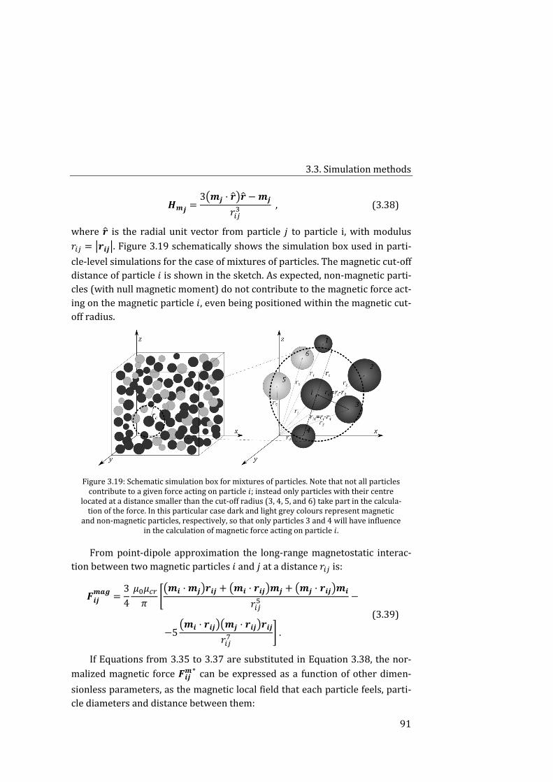
3.3. Simulation methods
91
𝑯𝒎𝒋=
3(𝒎𝒋 · �̂�)�̂� − 𝒎𝒋
𝑟𝑖𝑗3 , (3.38)
where �̂� is the radial unit vector from particle 𝑗 to particle i, with modulus
𝑟𝑖𝑗 = |𝒓𝒊𝒋|. Figure 3.19 schematically shows the simulation box used in parti-
cle-level simulations for the case of mixtures of particles. The magnetic cut-off
distance of particle 𝑖 is shown in the sketch. As expected, non-magnetic parti-
cles (with null magnetic moment) do not contribute to the magnetic force act-
ing on the magnetic particle 𝑖, even being positioned within the magnetic cut-
off radius.
Figure 3.19: Schematic simulation box for mixtures of particles. Note that not all particles contribute to a given force acting on particle 𝑖; instead only particles with their centre
located at a distance smaller than the cut-off radius (3, 4, 5, and 6) take part in the calcula-tion of the force. In this particular case dark and light grey colours represent magnetic
and non-magnetic particles, respectively, so that only particles 3 and 4 will have influence in the calculation of magnetic force acting on particle 𝑖.
From point-dipole approximation the long-range magnetostatic interac-
tion between two magnetic particles 𝑖 and 𝑗 at a distance 𝑟𝑖𝑗 is:
𝑭𝒊𝒋𝒎𝒂𝒈
=3
4
𝜇0𝜇𝑐𝑟
𝜋[(𝒎𝒊 · 𝒎𝒋)𝒓𝒊𝒋 + (𝒎𝒊 · 𝒓𝒊𝒋)𝒎𝒋 + (𝒎𝒋 · 𝒓𝒊𝒋)𝒎𝒊
𝑟𝑖𝑗5 −
−5(𝒎𝒊 · 𝒓𝒊𝒋)(𝒎𝒋 · 𝒓𝒊𝒋)𝒓𝒊𝒋
𝑟𝑖𝑗7 ] .
(3.39)
If Equations from 3.35 to 3.37 are substituted in Equation 3.38, the nor-
malized magnetic force 𝑭𝒊𝒋𝒎∗
can be expressed as a function of other dimen-
sionless parameters, as the magnetic local field that each particle feels, parti-
cle diameters and distance between them:
3. Methodology
92
𝑭𝒊𝒋𝒎∗
= 𝜎𝑖∗3
𝜎𝑗∗3
[(𝑯𝒍𝒐𝒄𝒊
∗ · 𝑯𝒍𝒐𝒄𝒋
∗ ) 𝒓𝒊𝒋∗ + (𝑯𝒍𝒐𝒄𝒊
∗ · 𝒓𝒊𝒋∗ )𝑯𝒍𝒐𝒄𝒋
∗
𝑟𝑖𝑗∗5 +
+(𝑯𝒍𝒐𝒄𝒋
∗ · 𝒓𝒊𝒋∗ ) 𝑯𝒍𝒐𝒄𝒊
∗
𝑟𝑖𝑗∗5 −5
(𝑯𝒍𝒐𝒄𝒊
∗ · 𝒓𝒊𝒋∗ ) (𝑯𝒍𝒐𝒄𝒋
∗ · 𝒓𝒊𝒋∗ ) 𝒓𝒊𝒋
∗
𝑟𝑖𝑗∗7 ] .
(3.40)
Repulsive interactions
In order to prevent particle overlap a repulsive Hertzian contact force is used
[57]. It considers mechanical properties of particles that take part in the con-
tact (Young’s modulus 𝐸 and Poisson’s ratio 𝜈) and it is calculated when there
exists particle overlap, i.e., when the distance between two particles
ℎ𝑖𝑗 = 𝑅𝑖 + 𝑅𝑗 − |𝒓𝒊𝒋| < 0. The radius of 𝑖 and 𝑗 particle are 𝑅𝑖 and 𝑅𝑗, respec-
tively. The Hertzian interaction is given by this expression:
𝑭𝒊𝒋𝒓 = (
4
3𝐸𝑒𝑓𝑓√𝑅𝑒𝑓𝑓ℎ
𝑖𝑗
32 ) �̂�𝒊𝒋 , (3.41)
where 𝐸𝑒𝑓𝑓 = ((1−𝜈𝑖
2)
𝐸𝑖+
(1−𝜈𝑗2)
𝐸𝑗)
−1
, 𝑅𝑒𝑓𝑓 =𝑅𝑖𝑅𝑗
𝑅𝑖+𝑅𝑗 and �̂�𝒊𝒋 =
𝒓𝒊𝒋
𝑟𝑖𝑗 is the unitary
vector in direction of 𝒓𝒊𝒋. In its dimensionless form, Equation 3.40 changes to:
𝑭𝒊𝒋𝒓 ∗
=1
3𝐸𝑒𝑓𝑓
∗√𝑅𝑒𝑓𝑓
∗ ℎ𝑖𝑗∗
32
𝒓𝒊𝒋∗
𝑟𝑖𝑗∗ . (3.42)
Wall interaction
The short-range wall force avoid particles to leave the simulation box in 𝑧-
direction as it simulates the upper and bottom plates that confine the sample
in experiments in parallel-plate configuration. This repulsive force has an ex-
ponential decay with particle separation as it is shown in next equation:
𝑭𝒊𝒘∗
= 𝑒−𝑘∗(ℎ𝑖∗−𝜎𝑖
∗/2) �̂� . (3.43)
Brownian force
The last contribution to the net force comes from Brownian motion, as
𝒇𝑩∗ ∝ √
𝑘𝐵𝑇
𝜎𝑚𝐹0
√𝜎𝑖
∗
∆𝑡∗ , (3.44)
where 𝑘𝐵 = 1.381 · 10−23 J · K−1 is the Boltzmann constant and 𝑇 the abso-
lute temperature expressed in kelvin.
3.3. Simulation methods
93
Simulation of mixtures of particles 3.3.2.
General description of the simulated system
Magnetorheological suspensions are treated as a mixture of monodisperse
(particle diameter of 𝜎 = 1 μm) magnetizable and non-magnetizable spheres
in a continuous phase with Newtonian viscosity 휂 = 1 mPa · s. 3D particle-
level simulations were carried out over a total number of particles of
𝑁 = 1000. The spheres are confined in a simulation box (see Figure 3.18) of
volume 𝑉 = 𝐿𝑥∗ × 𝐿𝑦
∗ × 𝐿𝑧∗ , which has a vertex coinciding with the origin of the
coordinate system. The total number of particles is related to this volume
through the particle volume fraction 𝜙𝑇 =𝜋𝜎3𝑁
6𝑉. Periodic boundary condi-
tions are used in 𝑥 and 𝑦-direction but not in 𝑧 as in the experimental case the
system is bounded by solid surfaces. Sticky boundary conditions are em-
ployed to mimic these surfaces, and the height of the simulation box in all
simulations was 𝐿𝑧∗ = 20. Asterisks denote dimensionless quantities, in this
case the length scale is the particle mean diameter 𝜎𝑚. Parameters used to
normalize each magnitude involved in this section are defined in Table 3.5.
Four total particle volume fractions were studied, namely 𝜙𝑇 = 0.05, 0.10,
0.20 and 0.30, so that dimensions 𝐿𝑥∗ and 𝐿𝑦
∗ of the simulation box change in
accordance to the total volume fraction in each case, as 𝐿𝑧∗ is fixed. The total
volume fraction is the sum of the magnetic 𝜙𝑀 and non-magnetic 𝜙𝑁 particle
volume fractions. Volume fractions of magnetic and nonmagnetic phases used
along this work are referred to the total volume fraction, so that they are in-
deed relative volume fractions 𝜙𝑖′, i.e., 𝜙𝑀
′ = 𝜙𝑀/𝜙𝑇, 𝜙𝑁′ = 𝜙𝑁/𝜙𝑇, and
𝜙𝑀′ + 𝜙𝑁
′ = 1. The number of magnetic particle in the simulation box was var-
ied between 50 and 1000 (i.e., 𝜙𝑀′ = 0.05 − 1). Simulation parameters are
shown in Table 3.6.
Each initial configuration of particles is generated by randomly placing
the 𝑁 particles in the simulation box (note that a smaller number of particles
𝑁 provided statistically irrelevant results with noisy data). Forces acting on
each particle are evaluated considering cut-off distances. At each simulation
time net forces are evaluated for each particle and the equation of motion is
solved. Then the particles are moved to their new positions and the process is
repeated for the next time steps. Five initial configurations were generated
for each mixture of particles (given by 𝜙𝑇 and 𝜙𝑀′ ) and averages of these runs
were performed.
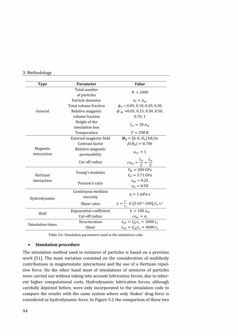
3. Methodology
94
Type Parameter Value
General
Total number
of particles 𝑁 = 1000
Particle diameter 𝜎𝑖 = 𝜎𝑚
Total volume fraction 𝜙𝑇 = 0.05, 0.10, 0.20, 0.30
Relative magnetic
volume fraction
𝜙′𝑀 =0.05, 0.15, 0.30, 0.50,
0.70, 1
Height of the
simulation box 𝐿𝑧 = 20 𝜎𝑚
Temperature 𝑇 = 298 K
Magnetic
interaction
External magnetic field 𝑯𝟎 = [0, 0, 𝐻0] kA/m
Contrast factor 𝛽(𝐻0) = 0.706
Relative magnetic
permeability 𝜇𝑐𝑟 = 1
Cut-off radius 𝑐𝑜𝑚 =𝐿𝑥
2=
𝐿𝑦
2
Hertzian
interaction
Young’s modulus
Poisson’s ratio
𝑌𝑀 = 200 GPa
𝑌𝑁 = 3.71 GPa
𝜈𝑀 = 0.25
𝜈𝑁 = 0.50
Hydrodynamic
Continuous medium
viscosity 휂 = 1 mPa·s
Shear rates �̇� =�̇�∗
𝑡𝑠 ∈ [3·10-3-100]/𝑡𝑠 s-1
Wall Exponential coefficient 𝑘 = 100 𝜎𝑚
Cut-off radius 𝑐𝑜𝑤 = 𝜎𝑖
Simulation times Structuration 𝑡𝑆𝑇 = 𝑡𝑆𝑇
∗ 𝑡𝑠 = 1000 𝑡𝑠
Shear 𝑡𝑆𝐻 = 𝑡𝑆𝐻∗ 𝑡𝑠 = 4000 𝑡𝑠
Table 3.6: Simulation parameters used in the simulation code.
Simulation procedure
The simulation method used in mixtures of particles is based on a previous
work [51]. The main variation consisted on the consideration of multibody
contributions in magnetostatic interactions and the use of a Hertzian repul-
sive force. On the other hand most of simulations of mixtures of particles
were carried out without taking into account lubrication forces, due to inher-
ent higher computational costs. Hydrodynamic lubrication forces, although
carefully depicted before, were only incorporated to the simulation code to
compare the results with the same system where only Stokes’ drag force is
considered as hydrodynamic force. In Figure 5.2 the comparison of these two
3.3. Simulation methods
95
cases is shown. In this sense, we considered that there was no risk in avoiding
the pairwise hydrodynamic interactions as magnetic forces prevail.
The simulation procedure consisted in two stages: structuration at rest
followed by a stage at constant shear, both in presence of an uniform magnet-
ic field 𝑯𝟎. The simulation time in the structuration step 𝑡𝑆𝑇∗ was long enough
for the system to show a steady state and magnetic particles to be arranged in
columnar aggregates. Once this simulation is completed the suspension is
subjected to several dimensionless shear rates �̇�∗ (in the range of 3 · 10−3 to
100) by means of considering a no null velocity field 𝒖𝒊∞∗
= �̇�∗𝑧𝑖∗�̂�, that is
added to the particle velocity due to the net force. The dimensionless shear
stress can be monitored with time in this stress growth test. The time evolu-
tion of stress in a start-up test provides a first region where the stress contin-
uously increases, as a consequence of an elastic deformation of the material,
up to a critical strain where a peak in the shear stress value is shown. It is the
so-called static yield stress. Then the shear stress reaches an equilibrium val-
ue at high strain deformations. The main contribution to the dimensionless
shear stress comes from the magnetic force, which is calculated following the
next expression:
𝜏𝑥𝑧𝑚∗ = −
1
𝑉∗∑ 𝑧𝑖
∗𝐹𝑥,𝑖𝑚∗
𝑁
𝑗≠𝑖
. (3.45)
For simplicity, the rest of non-hydrodynamic interactions acting on the
particles (repulsive, wall and Brownian forces) were not considered in the
calculation of the total stress, as their relative relevance compared to magne-
tostatic interactions was quite low. The total stress was obtained by adding
the hydrodynamic contribution from the applied shear to the static magnetic
stress. This option was preferred to adding the hydrodynamic contribution to
the equilibrium value of the magnetic stress as for low shear rates it takes
very long times to achieve the steady state value. However, the maximum is
well developed for each dimensionless shear rate in the range of selected
simulation times.
Yield stress has been calculated by fitting the curves in rheogram to Cas-
son model (√𝜏 = √𝜏𝑦 + √휂𝑝�̇�) and this value is compared to the yield stress
obtained by averaging shear stresses at lower shear rates.
3. Methodology
96
Squeeze simulations 3.3.3.
Brownian dynamics simulations were carried out to simulate systems of 1000
monodisperse spherical magnetic particles. The simulation code contains
three steps that are equivalent to the experimental protocol: particle structu-
ration, squeeze and shear, while considering a constant magnetic field of
𝐻0 = 177 kA · m−1 during the whole protocol. Both constant-volume and con-
stant-area squeeze tests were simulated.
The volume fraction was varied among 𝜙 = 0.05 and 0.30. We used peri-
odic boundary conditions in 𝑥 and 𝑦 directions, and two initial gaps ℎ𝑖∗ were
studied, namely 20 and 30 times the mean diameter 𝜎𝑚, which is employed as
a length scale. So that, depending on the initial gap and the volume fraction,
the other two dimensions of the simulation box can be easily determined. Par-
ticles are randomly distributed in the simulation box and overlap is forbid-
den. The magnetic dipoles of the particles are supposed to be equal at the on-
set of the simulation and oriented with the magnetic field, it is, in 𝑧 axis.
Local magnetic field (Equations from 3.35 to 3.39) is considered in the
calculation of the magnetic force between pairs of particles. In this sense, for a
given particle its magnetic force is due both to the external magnetic field and
the rest of contributions from other particles that surround it at distances
lower than a stablished cut-off. Apart from magnetic interactions, Stoke’s drag
(Equation 3.21) and Brownian forces (Equation 3.43) are taken into account,
as well as an exponential repulsive force (Equation 3.45) that decays with
particle separation as expressed below:
𝑭𝒊𝒋𝒓 = 𝐹0𝑒−𝑘(𝑟𝑖𝑗−(𝑑𝑖+𝑑𝑗)/2)�̂�𝒊𝒋 , (3.46)
where 𝐹0 is the force scale (see Table 3.5), 𝑘 = 100 and 𝑟𝑖𝑗is the center-to-
center distance between particles 𝑖 and 𝑗. Besides, all forces are not consid-
ered in squeeze simulations.
The Langevin equation if inertia is neglected (Equation 3.17) is solved at
each time step and the new particle positions are considered in the next time
step. In the structuration step the main contribution to the particle move-
ments comes from magnetic interactions. The normalized time for structu-
ration is sufficient to obtain steady states in the magnetic energy, normal
stress, normal force and number of neighbours. After that, the particle config-
uration is subjected to the squeeze step, in which the gap is steadily forced to
diminish at a given velocity, and so the height of the simulation box. The time
3.3. Simulation methods
97
during which the gap diminishes depends on the required level of defor-
mation. In constant-volume simulations it provokes an enlargement in the
other dimensions of the simulation box, so that particles have to fit in a modi-
fied simulation box that keeps the initial volume and, as a consequence, the
volume fraction does not vary. On the contrary, in constant-area simulations
the gap is diminished, while the other two dimensions preserve their initial
lengths so that the simulation box is smaller. As it occurs in the experimental
case, particles are confined in the area subjected to the magnetic field and
cannot abandon the new simulation box, so that the volume fraction increases
with 휀 in constant-area conditions. Once a given deformation is achieved, the
shear flow is activated at constant shear rates. The effect of the compression
of the magnetic structures in the static yield stress under shear is compared
for both types of simulations.
EHL simulations 3.3.4.
We followed two methods to calculate the friction coefficient using numerical
simulations: i) a “simplified” solution approach and ii) a “full” solution ap-
proach. The notation of dimensional and dimensionless parameters used in
EHL simulations is shown in Table 3.7 and Table 3.8, respectively.
In the simplified solution approach the lubricant was considered to be a
Newtonian fluid, at a local scale, and regression formulas were used to predict
the friction coefficient. In the contact, an effective shear viscosity was esti-
mated using an iterative procedure from the lubricant’s rheogram under
steady shear. In the full solution approach, by a means of the finite-difference
method, we solved the generalized Reynolds equation coupled with the load
balance equation and the surface elastic deformation equation. From the full
solution, regression equations are proposed for the prediction of the film
thickness and friction coefficients for both shear-thinning and shear-
thickening fluids.
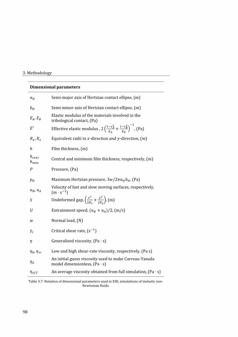
3. Methodology
98
Dimensional parameters
𝑎𝐻 Semi-major axis of Hertzian contact ellipse, (m)
𝑏𝐻 Semi-minor axis of Hertzian contact ellipse, (m)
𝐸𝐴, 𝐸𝐵 Elastic modulus of the materials involved in the tribological contact, (Pa)
𝐸′ Effective elastic modulus , 2 (1−𝜈𝐴
2
𝐸𝐴+
1−𝜈𝐵2
𝐸𝐵)
−1
, (Pa)
𝑅𝑥 , 𝑅𝑥 Equivalent radii in 𝑥-direction and 𝑦-direction, (m)
ℎ Film thickness, (m)
ℎ𝑐𝑒𝑛, ℎ𝑚𝑖𝑛
Central and minimum film thickness, respectively, (m)
𝑃 Pressure, (Pa)
𝑝𝐻 Maximum Hertzian pressure, 3𝑤/2𝜋𝑎𝐻𝑏𝐻, (Pa)
𝑢𝐵, 𝑢𝐴 Velocity of fast and slow moving surfaces, respectively, (m · s−1)
𝑆 Undeformed gap, (𝑥2
2𝑅𝑥+
𝑦2
2𝑅𝑦), (m)
𝑈 Entrainment speed, (𝑢𝐵 + 𝑢𝐴)/2, (m/s)
𝑤 Normal load, (N)
�̇�𝑐 Critical shear rate, (s−1)
휂 Generalized viscosity, (Pa · s)
휂0, 휂∞ Low and high shear-rate viscosity, respectively, (Pa s)
휂𝐺 An initial guess viscosity used to make Carreau-Yasuda model dimensionless, (Pa · s)
휂𝑒𝑓𝑓 An average viscosity obtained from full simulation, (Pa · s)
Table 3.7: Notation of dimensional parameters used in EHL simulations of inelastic non-Newtonian fluids.
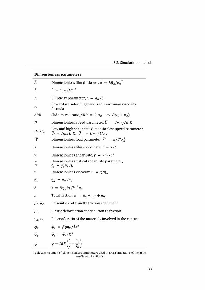
3.3. Simulation methods
99
Dimensionless parameters
ℎ̅ Dimensionless film thickness, ℎ̅ = ℎ𝑅𝑥/𝑏𝐻2
𝐼�̅� 𝐼�̅� = 𝐼𝑛휂𝐺 ℎ𝑛+1⁄
𝐾 Ellipticity parameter, 𝐾 = 𝑎𝐻 𝑏𝐻⁄
𝑛 Power-law index in generalized Newtonian viscosity formula
𝑆𝑅𝑅 Slide-to-roll ratio, 𝑆𝑅𝑅 = 2|𝑢𝐵 − 𝑢𝐴|/(𝑢B + 𝑢A)
�̅� Dimensionless speed parameter, �̅� = 𝑈휂𝑒𝑓𝑓 𝐸′𝑅𝑥⁄
�̅�0, �̅�∞ Low and high shear rate dimensionless speed parameter, �̅�0 = 𝑈휂0 𝐸′𝑅𝑥⁄ , �̅�∞ = 𝑈휂∞ 𝐸′𝑅𝑥⁄
�̅� Dimensionless load parameter, �̅� = 𝑤/𝐸′𝑅𝑥2
𝑧̅ Dimensionless film coordinate, 𝑧̅ = 𝑧 ℎ⁄
�̅̇� Dimensionless shear rate, �̇� ̅ = �̇�휂𝐺/𝐸′
�̅̇�𝑐 Dimensionless critical shear rate parameter, �̅̇�𝑐 = �̇�𝑐𝑅𝑥 𝑈⁄
휂̅ Dimensionless viscosity, 휂̅ = 휂/휂𝐺
휂̅𝑅 휂̅𝑅 = 휂∞ 휂0⁄
�̅� λ̅ = 𝑈휂𝐺𝑅𝑥2/𝑏𝐻
3𝑝𝐻
𝜇 Total friction, 𝜇 = 𝜇𝑃 + 𝜇𝐶 + 𝜇𝐷
𝜇𝑃 , 𝜇𝐶 Poiseuille and Couette friction coefficient
𝜇𝐷 Elastic deformation contribution to friction
𝜈𝐴, 𝜈𝐵 Poisson’s ratio of the materials involved in the contact
�̅�𝑥 �̅�𝑥 = �̅�𝜙휂𝐺 �̅�ℎ3⁄
�̅�𝑦 �̅�𝑦 = �̅�𝑥 𝐾2⁄
�̅� �̅� = 𝑆𝑅𝑅 (1
2−
Π̅1
𝐼0̅)
Table 3.8: Notation of dimensionless parameters used in EHL simulations of inelastic non-Newtonian fluids.
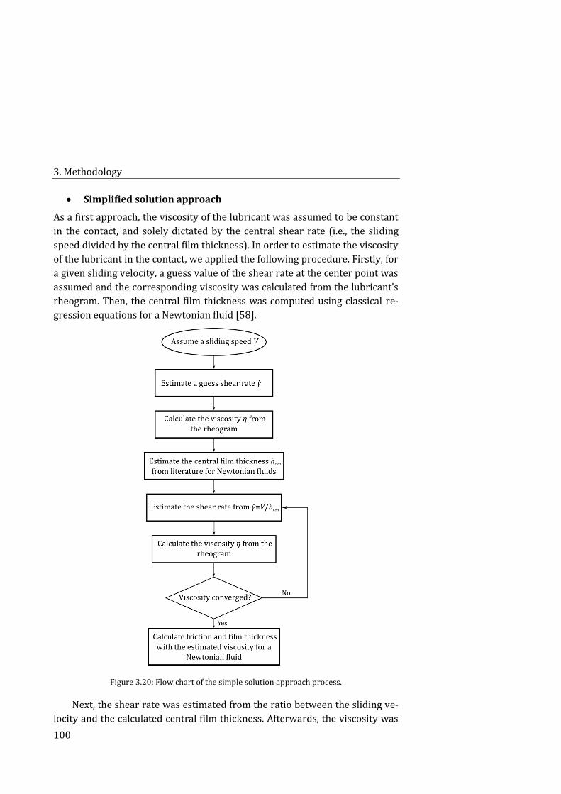
3. Methodology
100
Simplified solution approach
As a first approach, the viscosity of the lubricant was assumed to be constant
in the contact, and solely dictated by the central shear rate (i.e., the sliding
speed divided by the central film thickness). In order to estimate the viscosity
of the lubricant in the contact, we applied the following procedure. Firstly, for
a given sliding velocity, a guess value of the shear rate at the center point was
assumed and the corresponding viscosity was calculated from the lubricant’s
rheogram. Then, the central film thickness was computed using classical re-
gression equations for a Newtonian fluid [58].
Figure 3.20: Flow chart of the simple solution approach process.
Next, the shear rate was estimated from the ratio between the sliding ve-
locity and the calculated central film thickness. Afterwards, the viscosity was
3.3. Simulation methods
101
computed for the calculated shear rate from the prescribed rheogram. In the
next step, the calculated viscosity was compared to the initial guess viscosity.
If the difference was small, the viscosity was accepted as the final value. Oth-
erwise, the viscosity obtained from the rheogram was considered as a new
guess value and the iteration was repeated until convergence reached. Finally,
the viscosity obtained from this simple approach was used to estimate both
Couette and Poiseuille friction terms using regression formulas [59] for a
Newtonian fluid (see Equations from 3.52 to 3.54 below). The flow chart cor-
responding to this simple solution approach is shown in Figure 3.20:
Full solution approach
The generalized Reynolds equation for the case of an I-EHL point contact lu-
bricated by an inelastic incompressible non-Newtonian fluid at steady-state is
given by [60,61]:
𝜕
𝜕𝑥(𝜙
𝜕𝑝
𝜕𝑥) +
𝜕
𝜕𝑦(𝜙
𝜕𝑝
𝜕𝑦) = 𝑈
𝜕
𝜕𝑥[ℎ(1 + 𝜓)] . (3.47)
The lubricant flow is contained in the 𝑥𝑦 plane and the film thickness
points along the 𝑧-direction. 𝑈 = (𝑢𝐵 + 𝑢𝐴)/2 is the entrainment speed in the
flow direction and 𝑢𝐵 and 𝑢𝐴 denotes the velocity of the two shearing surfaces
in the 𝑥-direction for the fast and slow moving surfaces, respectively. The en-
trainment speed in 𝑦-direction is zero (𝑣𝐵 = 𝑣𝐴 = 0). The integral functions
in Equation 3.46 are given by 𝜙 = ∫𝑧
𝜂(𝑧 −
𝐼1
𝐼0) 𝑑𝑧
ℎ
0 and 𝜓 = 𝑆𝑅𝑅 (
1
2−
Π1
𝐼0
1
ℎ),
where Π1 = ∫𝑧
𝜂𝑑𝑧
ℎ
0 and 𝐼𝑛 = ∫
𝑧𝑛
𝜂𝑑𝑧
ℎ
0. Here, 𝑆𝑅𝑅 is the slide-to-roll ratio. For
a Newtonian fluid Π1
𝐼0=
𝐼1
𝐼0=
ℎ
2, 𝜓 = 0, and 𝜙 =
ℎ3
12𝜂. Hence, for a Newtonian flu-
id (seeEquation 3.46) reduces to the classical Reynolds equation.
The generalized Reynolds equation has to be solved simultaneously with
the elastic deformation equation
𝐷(𝑥, 𝑦) =2
𝜋𝐸′∫ ∫
𝑝𝑑𝑥′𝑑𝑦′
√(𝑥′ − 𝑥)2 + (𝑦′ − 𝑦)2 , (3.48)
and the force balance equation over the solution domain Ω
∬ 𝑝𝑑𝑥𝑑𝑦 = 𝑤Ω
. (3.49)
The film thickness is given by summation of the undeformed gap between
the surfaces and the elastic deformation as follows:
3. Methodology
102
ℎ(𝑥, 𝑦) = ℎ0 + 𝑆(𝑥, 𝑦) + 𝐷(𝑥, 𝑦) , (3.50)
where ℎ0 is a constant that determines the distance between two remote
points in the solids and 𝑆(𝑥, 𝑦) is the parabolic approximation of the unde-
formed gap. The Reynolds equation (Equation 3.46) was transformed into a
dimensionless form using the parameters given in Table 3.8 as follows:
𝜕
𝜕�̅�(�̅�𝑥
𝜕�̅�
𝜕�̅�) +
𝜕
𝜕�̅�(�̅�𝑦
𝜕𝑝
𝜕𝑦) =
𝜕
𝜕�̅�(�̅�ℎ̅(1 + �̅�)) +
𝜕
𝜕𝑡̅(�̅�ℎ̅) . (3.51)
Rheological constitutive equation of the lubricant
In the I-EHL regime, the elastic deformation of the solids is substantial if
compared to the film thickness of the lubricant separating the surfaces. How-
ever, the contact pressure is low enough to invoke any significant change in
the lubricant viscosity. Therefore, the effect of pressure on the lubricant vis-
cosity is negligible. Nevertheless, in the case of inelastic non-Newtonian fluids
it is necessary to take into account the shear rate dependence of the viscosity
to adequately predict the film thickness and the pressure distribution in the
contact. Here, the viscosity of the lubricant was modelled using the double-
Newtonian Carreau-Yasuda expression:
휂 = 휂∞ +휂0 − 휂∞
[1 + (�̇��̇�𝑐
)2
]
1−𝑛2
, (3.52)
where 휂0 and 휂∞ denote the low and high shear viscosity plateau, respective-
ly. �̇� = ‖𝑑𝑢
𝑑𝑧‖ is the magnitude of the shear rate tensor; note that
𝑑𝑣
𝑑𝑧 is zero.
The velocity gradient across the film thickness is 𝑑𝑢
𝑑𝑧=
1
𝜂[
𝜕𝑝
𝜕𝑥(𝑧 −
𝐼1
𝐼0) +
𝑈∙𝑆𝑅𝑅
𝐼0].
�̇�𝑐 is a critical shear rate that defines the departure from the low-shear viscos-
ity region and the onset of the power-law region. 𝑛 is the viscosity index and
determines the slope of the viscosity in the transition region. For the special
case of a zero second Newtonian viscosity, the slope of power-law is given
by 𝑛 − 1.
According to Equation 3.50, either 𝑛 = 1 or 휂0 = 휂∞ denote Newtonian
fluids. For 𝑛 ≠ 1, the fluid is shear thinning if 휂∞ < 휂0, and shear-thickening
if 휂0 < 휂∞. A lower value of the viscosity index 𝑛, i.e., higher slope, implies a
sharper change from the low shear to the high shear viscosity regions, which
means a stronger shear-thickening/thinning behaviour.
3.3. Simulation methods
103
Numerical procedure
In order to numerically solve Equation 3.49 we used a hybrid line relaxation
method [62], with a central second order discretization for the Poiseuille
term and an upstream second order discretization for the wedge/squeeze
term. The integration was performed across the film thickness using Simp-
son’s rule with 18 mesh points. The simulation began with an initial guess for
the pressure 𝑝𝐺 (in particular, a Hertzian dry contact distribution with
us 𝑎𝐻), approaching distance ℎ0 and viscosity guess 휂𝐺 . 𝑝𝐺 and ℎ0 were up-
dated during relaxation but 휂𝐺 was only used for transforming Reynolds
equation into dimensionless form and was kept constant. Independently of
the initial 휂𝐺 , the procedure converged to a unique solution. However, a good
guess value, close to the final viscosity solution at the central point, accelerat-
ed the convergence.
The numerical procedure was as follows. (i) At each mesh point in the
computational domain, an average viscosity was obtained by iteration at 18
nodes across the film thickness using Simpson’s rule. Then, the integral func-
tions 𝐼0̅, 𝐼1̅, and 𝛱1 were evaluated at each mesh point in the computational
domain. The parameters �̅�𝑥, �̅�𝑦, �̅� were computed and the pressure was up-
dated iteratively using a hybrid line relaxation scheme until the relative error
in pressure was below 10−4. (ii) Next, the relative error in the normal load
was calculated and the load equilibrium equation (Equation 3.47) was used to
correct the approaching distance. (iii) The loops (i) and (ii) were repeated
until reaching a relative error less than 10−4 in both pressure and load. To
ensure fully-flooded conditions with a uniform mesh, the computational do-
main had a size of 4𝑎𝐻 in the inlet and 2𝑎𝐻 in the outlet region.
Simulations were carried out at different values of viscosity index (𝑛),
low-shear-rate viscosity (휂0), high-shear-rate viscosity (휂∞), critical shear
rate (�̇�𝑐), slide-to-roll ratio (𝑆𝑅𝑅), entrainment speed (𝑈), and normal load
(𝑤) for each lubricant.
Friction coefficient calculation
Rolling and sliding are two mechanisms that are responsible for the transfer
of frictional stresses between two contacting lubricated surfaces [63]. Adhe-
sion of the contacting asperities at low velocities and the Couette flow of the
lubricant film in the contact at large velocities are the two main sources of
sliding friction. Furthermore, the rolling friction has two main components,
one contribution arising from deformation/elastic hysteresis [64], and the
3. Methodology
104
other one coming from Poiseuille flow of the lubricant in the contact at large
velocities. Since interfacial adhesion is negligible when surfaces are separated
by fluid film, Couette 𝜇𝐶 , Poiseuille 𝜇𝑃 , and elastic hysteresis 𝜇𝐷 terms are the
only three contributions that are needed to determine the total friction coeffi-
cient 𝜇 in the hydrodynamic regime.
From the solution of the generalized Reynolds equations and the elastic
deformation equations (Equation 3.46 and 3.47, respectively), both Couette
𝜏𝐶 and Poiseuille 𝜏𝑃 contributions to the shear stress, over the fast moving
surface, can be obtained as follows:
𝜏𝐶 = −𝑆𝑅𝑅 ∙ 𝑈
𝐼0 , (3.53)
𝜏𝑃 = −𝜕𝑝
𝜕𝑥(ℎ −
𝐼1
𝐼0) . (3.54)
Furthermore, in the particular case of a sphere-on-flat contact, the fric-
tion coefficient contribution coming from elastic hysteresis (i.e., deformation
energy losses) can be estimated as follows [63]:
𝜇𝐷 = 𝛼3
16
𝑎𝐻
𝑅 , (3.55)
where 𝑅 is the sphere radius and 𝛼 is the loss factor. The loss factor is given
by 𝛼 = 𝑘𝜋tan(𝛿) where 𝑘 is a constant in the range of 1-3 and the loss tangent
tan(𝛿) is reported to be 0.11 for PDMS tribopairs [64].
In the particular case of Newtonian fluids, regression equations were ob-
tained in [59] for both Couette and Poiseuille contributions to the friction co-
efficient. The regression equations are:
𝜇C = 𝑆𝑅𝑅(3.8�̅�0.71�̅�−0.76 + 0.96�̅�0.36�̅�−0.11) , (3.56)
𝜇P = 1.46�̅�0.65�̅�−0.70 . (3.57)
These two equations together with Equation 3.54 were used in the sim-
plified solution approach to predict the friction coefficient.
References 3.4.
[1] BeMiller J N and Huber K C 2011 Starch Ullmann’s Encyclopedia of In-dustrial Chemistry (Wiley-VCH Verlag GmbH & Co. KGaA)
[2] Bertoft E 2017 Understanding starch structure: recent progress Agronomy 7 56
3.4. References
105
[3] Vamadevan V and Bertoft E 2014 Structure-function relationships of starch components Starch - Stärke 67 55–68
[4] BeMiller J N and Whistler R L 2009 Starch: chemistry and technology (London: Academic Press)
[5] Pratsinis S E 1998 Flame aerosol synthesis of ceramic powders Prog. Energy Combust. Sci. 24 197–219
[6] Flörke O W, Graetsch H A, Brunk F, Benda L, Paschen S, Bergna H E, Roberts W O, Welsh W A, Libanati C, Ettlinger M, Kerner D, Maier M, Meon W, Schmoll R, Gies H and Schiffmann D 2008 Silica Ullmann’s Encyclopedia of In-dustrial Chemistry ed Wiley-VCH Verlag GmbH & Co. KGaA (Weinheim, Ger-many: Wiley-VCH Verlag GmbH & Co. KGaA)
[7] Raghavan S R and Khan S A 1997 Shear-thickening response of fumed silica suspensions under steady and oscillatory shear J. Colloid Interface Sci. 185 57–67
[8] Raghavan S R, Walls H J and Khan S A 2000 Rheology of silica disper-sions in organic liquids: new evidence for solvation forces dictated by hydro-gen bonding Langmuir 16 7920–7930
[9] Warren J, Offenberger S, Toghiani H, Pittman C U, Lacy T E and Kundu S 2015 Effect of temperature on the shear-thickening behavior of fumed sili-ca suspensions ACS Appl. Mater. Interfaces 7 18650–18661
[10] Royer J R, Blair D L and Hudson S D 2016 Rheological signature of fric-tional interactions in shear thickening suspensions Phys. Rev. Lett. 116
[11] de Vicente J, Klingenberg D J and Hidalgo-Álvarez R 2011 Magne-torheological fluids: a review Soft Matter 7 3701
[12] Ashour O, Rogers C A and Kordonsky W 1996 Magnetorheological flu-ids: materials, characterization, and devices J. Intell. Mater. Syst. Struct. 7 123–30
[13] Bombard A J F, Knobel M, Alcantara M R and Joekes I 2002 Evaluation of magnetorheological suspensions based on carbonyl iron powders J. Intell. Mater. Syst. Struct. 13 471–478
[14] Ashtiani M, Hashemabadi S H and Ghaffari A 2015 A review on the magnetorheological fluid preparation and stabilization J. Magn. Magn. Mater. 374 716–730
[15] Boczkowska A, Awietjan S F, Pietrzko S and Kurzydłowski K J 2012 Mechanical properties of magnetorheological elastomers under shear defor-mation Compos. Part B Eng. 43 636–40
3. Methodology
106
[16] Jolly M R, Carlson J D, Muñoz B C and Bullions T A 1996 The magne-toviscoelastic response of elastomer composites consisting of ferrous parti-cles embedded in a polymer matrix J. Intell. Mater. Syst. Struct. 7 613–622
[17] Choi H J, Park B J, Cho M S and You J L 2007 Core-shell structured poly(methyl methacrylate) coated carbonyl iron particles and their magne-torheological characteristics J. Magn. Magn. Mater. 310 2835–7
[18] Fang F F and Choi H J 2007 Polymeric nanobead coated carbonyl iron particles and their magnetic property Phys. Status Solidi A 204 4190–3
[19] Ulicny J C, Snavely K S, Golden M A and Klingenberg D J 2010 Enhanc-ing magnetorheology with nonmagnetizable particles Appl. Phys. Lett. 96 231903
[20] Klingenberg D J and Ulicny J C 2011 Enhancing magnetorheology Int. J. Mod. Phys. B 25 911–917
[21] Powell L A, Wereley N M and Ulicny J 2012 Magnetorheological fluids employing substitution of nonmagnetic for magnetic particles to increase yield stress IEEE Trans. Magn. 48 3764–3767
[22] Abdoulaye Fall 2008 Rhéophysique des fluides complexes: Ecoulement et Blocage de suspensions concentrées (Université Paris 7)
[23] Merkt F S, Deegan R D, Goldman D I, Rericha E C and Swinney H L 2004 Persistent holes in a fluid Phys. Rev. Lett. 92
[24] de Vicente J, Stokes J R and Spikes H A 2005 Lubrication properties of non-adsorbing polymer solutions in soft elastohydrodynamic (EHD) contacts Tribol. Int. 38 515–26
[25] Garrec D A and Norton I T 2012 The influence of hydrocolloid hydro-dynamics on lubrication Food Hydrocoll. 26 389–397
[26] Ruiz-López J A, Hidalgo-Alvarez R and de Vicente J 2016 A microme-chanical model for magnetorheological fluids under slow compression Rheol. Acta 55 215–21
[27] Macosko C W 1994 Rheology: principles, measurements, and applica-tions (New York: VCH)
[28] Steffe J F 1992 Rheological methods in food process engineering (East Lansing, Mich. USA: Freeman Press)
[29] Dzuy N Q and Boger D V 1985 Direct yield stress measurement with the vane method J. Rheol. 29 335–47
[30] Rabia A, Yahiaoui S, Djabourov M, Feuillebois F and Lasuye T 2014 Optimization of the vane geometry Rheol. Acta 53 357–371
3.4. References
107
[31] R. J. Poole 2016 Measuring normal-stresses in torsional rheometers: a practical guide. Rheol. Bull. 57 (2) 36–46
[32] López-López M T, Kuzhir P, Caballero-Hernández J, Rodríguez-Arco L, Duran J D G and Bossis G 2012 Yield stress in magnetorheological suspen-sions near the limit of maximum-packing fraction J. Rheol. 56 1209
[33] Vagberg D and Tighe B P 2017 On the apparent yield stress in non-Brownian magnetorheological fluids Soft Matter 13 7207–7221
[34] Morillas J R and de Vicente J 2019 Yielding behavior of model magne-torheological fluids Soft Matter 15 3330–42
[35] Barnes H A and Walters K 1985 The yield stress myth? Rheol. Acta 24 323–6
[36] Barnes H A 1999 The yield stress—a review or "παντα ρει"—everything flows? J. Non-Newton. Fluid Mech. 81 133–178
[37] Bonn D and Denn M M 2009 Yield stress fluids slowly yield to analysis Science 324 1401–2
[38] Dinkgreve M, Denn M M and Bonn D 2017 “Everything flows?”: elastic effects on startup flows of yield-stress fluids Rheol. Acta 56 189–194
[39] Moller P, Fall A, Chikkadi V, Derks D and Bonn D 2009 An attempt to categorize yield stress fluid behaviour Philos. Trans. R. Soc. Math. Phys. Eng. Sci. 367 5139–55
[40] Coussot P 2014 Yield stress fluid flows: A review of experimental data J. Non-Newton. Fluid Mech. 211 31–49
[41] Ovarlez G, Cohen-Addad S, Krishan K, Goyon J and Coussot P 2013 On the existence of a simple yield stress fluid behavior J. Non-Newton. Fluid Mech. 193 68–79
[42] Dinkgreve M, Paredes J, Denn M M and Bonn D 2016 On different ways of measuring “the” yield stress J. Non-Newton. Fluid Mech. 238 233–241
[43] Barnes H 1996 A review of the slip (wall depletion) of polymer solu-tions, emulsions and particle suspensions in viscometers: its cause, character, and cure Int. J. Multiph. Flow 22 132
[44] Cloitre M and Bonnecaze R T 2017 A review on wall slip in high solid dispersions Rheol. Acta 56 283–305
[45] Yoshimura A and Prud’homme R K 1988 Wall slip corrections for Couette and parallel disk viscometers J. Rheol. 32 53–67
[46] Ahmed H. Helal 2016 Designing devices using electro-active yield stress fluids (Massachusetts Institute of Technology)
3. Methodology
108
[47] Babick F 2016 Suspensions of colloidal particles and aggregates (Springer International Publishing)
[48] Malvern Instruments 2003 Zetasizer Nano Series: User Manual (MAN0317)
[49] Hunter R J 1981 The calculation of zeta potential Zeta Potential in Col-loid Science (Elsevier) pp 59–124
[50] Hebbar R S, Isloor A M and Ismail A F 2017 Contact angle measure-ments Membrane Characterization (Elsevier) pp 219–255
[51] Fernández-Toledano J C, Ruiz-López J A, Hidalgo-Álvarez R and de Vi-cente J 2015 Simulations of polydisperse magnetorheological fluids: A struc-tural and kinetic investigation J. Rheol. 59 475–98
[52] Ruiz-López J A, Hidalgo-Álvarez R and Vicente J de 2016 A microme-chanical model for magnetorheological fluids under slow compression Rheol. Acta 55 215–221
[53] Lagger H G, Breinlinger T, Korvink J G, Moseler M, Renzo A D, Maio F D and Bierwisch C 2015 Influence of hydrodynamic drag model on shear stress in the simulation of magnetorheological fluids J. Non-Newton. Fluid Mech. 218 16–26
[54] Lagger H G, Breinlinger T, Korvink J G, Moseler M, Di A, Di F and Bier-wisch C 2015 Influence of hydrodynamic drag model on shear stress in the simulation of magnetorheological fluids J. NON-Newton. FLUID Mech. 218 16–26
[55] Sangtae Kim S J K 1991 Microhydrodynamics (Elsevier)
[56] Martin J E and Anderson R A 1996 Chain model of electrorheology J. Chem. Phys. 104 4814–4827
[57] Lagger H G, Bierwisch C, Korvink J G and Moseler M 2014 Discrete el-ement study of viscous flow in magnetorheological fluids Rheol. Acta 53 417–43
[58] Hamrock B, Schmid S and Jacobson B 2004 Fundamentals of fluid film lubrication (CRC Press)
[59] de Vicente J, Stokes J R and Spikes H A 2005 The frictional properties of Newtonian fluids in rolling–sliding soft-EHL contact Tribol. Lett. 20 273–86
[60] Katyal P and Kumar P 2014 On the role of second Newtonian viscosity in EHL point contacts using double Newtonian shear-thinning model Tribol. Int. 71 140–148
[61] Dowson D 1962 A generalized Reynolds equation for fluid-film lubri-cation Int. J. Mech. Sci. 4 159–170
3.4. References
109
[62] Shahrivar K and de Vicente J 2014 Ferrofluid lubrication of compliant polymeric contacts: effect of non-homogeneous magnetic fields Tribol. Lett. 56 281–92
[63] Myant C, Spikes H A and Stokes J R 2010 Influence of load and elastic properties on the rolling and sliding friction of lubricated compliant contacts Tribol. Int. 43 55–63
[64] Timm K, Myant C, Spikes H A and Grunze M 2011 Particulate lubri-cants in cosmetic applications Tribol. Int. 44 1695–1703


II Results and discussion

113
4. Shear thickening in unimodal
suspensions
Introduction 4.1.
Suspensions of solid particles present a non-linear behaviour, which is de-
pendent on many factors such as the chemical and physical particle features,
their interactions with the fluid, the total and relative volume fraction in case
of hybrid systems, or external fields. The majority of these suspensions pre-
sent a shear-thinning behaviour, in which their resistance to flow decreases
with the shear rate. However, in the case of highly concentrated systems the
suspensions can exhibit shear thickening (ST), which is an increase in viscosi-
ty with the applied shear rate or stress [1–3], so that ST fluids are a type of
non-Newtonian fluid. These counter-intuitive fluids are commonly prepared
in Newtonian carriers where colloidal and nonaggregating particles are dis-
persed or suspended at moderate or high concentrations, such as cornstarch,
silica or calcium carbonate, among others [4]. Apart from these simple formu-
lations, some additives can be incorporated to obtain a smart fluid with a
combined response [5–9]. Among them, the use of magnetic particles leads to
a multi-phase system that is called magnetorheological shear-thickening fluid
(MRSTF) [10,11], which may exhibit both shear-thickening and magnetorheo-
logical effects. Thus, the rheological behaviour of these bimodal smart mate-
4. Shear thickening in unimodal suspensions
114
rials can be modulated by means of the applied magnetic field and the loading
conditions. However, to the authors’ knowledge the formulation of shear-
thickening fluids uniquely fabricated with unimodal magnetic particles has
been scarcely studied [12]. Moreover, this concentrated magnetorheological
fluid could, a priori, be modelled easily compared to mixtures of particles.
The phenomenon of shear thickening is an important concern in indus-
trial processes and the applications of these complex fluids are related to en-
ergy dissipation systems, such as dampers, sandwich structures and body
armour [13]. The amount of energy that can be dissipated in form of heat
through the fluid is proportional to its viscosity, so that a higher viscosity (ei-
ther by passive or field-active fluids) implies a better selectivity. Both the on-
set and intensity of this regime can be tuned with the precise knowledge in
suspension rheology. This fact would help us to adapt the fluid conditions to
our necessities for each practical application.
One of the earliest works on the shear-thickening behaviour correspond
to Metzner and Whitlock [14], who compiled all the available quantitative da-
ta on dilatancy (volume expansion). For his part, Barnes [15] concluded in his
review that in the appropriate range of shear rate a concentrated suspension
of nonaggregating solid particles would always result in reversible shear-
thickening behaviour. Although the terms shear thickening and dilatancy are
connected and were used as synonyms, dilatancy is necessary but not suffi-
cient for observing a strong shear thickening.
Scientists have been trying to understand the mechanisms which lead the
shear-thickening phenomenon for decades. Hoffman [16] developed a mi-
cromechanical model of ST as a flow-induced order-disorder transition,
which involves particles of the suspensions being in a layered orientation that
is disrupted as a consequence of increasing hydrodynamic forces acting on
the particles. Other researchers supported the concept of the formation of
transient arrangements of particles, called hydroclusters, that develop at
strong flow conditions and lead to increased lubrication drag forces between
particles [17]. Other mechanism that could lead shear thickening is dilation,
as it appeared in the pioneering works of Metzner and Whitlock, in which
both phenomena were thought as only one. Dilation recovered attention
again after the work of Brown and Jaeger [18]. They established that in con-
ditions of confinement that may frustrate the dilation of the suspension, a re-
storing force is transmitted along the system by means of frictional interac-
tions which would enable a dramatic increase in viscosity. Among these
4.1. Introduction
115
mechanisms, the hydroclusters theory was broadly though to be the main re-
sponsible for the occurrence of this phenomenon up to the recent idea of a
transition from hydrodynamically lubricated to frictional contacts. In fact, a
purely hydrodynamic effect provokes a mild ST (known as continuous, CST)
in less densely packed systems, but it is not sufficient to give rise to the strong
or discontinuous shear thickening (DST) occurring when the volume fraction
approaches the maximum packing fraction. Nowadays, new advances and im-
provements in computational methods are permitting very good agreements
with experimental results when considering friction as an important ingredi-
ent in the appearance of shear thickening. Thanks to that, both continuous
and discontinuous shear thickening are being reproduced in a satisfactory
manner [19–22].
The arrangement of particles in a suspension evolves when it is subjected
to shear, according to the predominant contributions to the stress at each
stage. At rest, particles will move randomly as Brownian motion dominates
the total force on the colloid, resulting in an isotropic microstructure. When
the suspension is subjected to shear flow, hydrodynamic forces gain rele-
vance and microstructural changes occur in the suspension, which becomes
anisotropic. However, if concentration and shear rates are high enough, fric-
tional contact networks are formed because of a predominant frictional con-
tribution [19,23,24], compared to the hydrodynamic interactions. In terms of
the first normal stress difference 𝑁1 (see Subsection 3.2.1), moderate shear
rates result in negative values of this parameter, while when the role played
by friction is significant enough, this leads to a transition in the sign of 𝑁1,
from negative to positive, which means that dilation is taking place.
In this work we address the study of the rheological behaviour of concen-
trated suspensions subjected to shear flow. The first approach to the shear-
thickening behaviour was carried out by considering model shear-thickening
colloids based on starch or fumed silica particles. Due to the strong coupling
with shear stress, special attention will be paid to the normal force evolution
in the shear-thickening region. The evolution of the viscosity and normal
force behaviour, as well as the differences found between both types of sys-
tems, is explained in terms of the type of particle involved in each suspension,
its deformability and roughness. The second part is devoted to the shear-
thickening response in concentrated magnetorheological suspensions. In this
sense, several volume fractions, carrier fluids and magnetic field strengths
were explored. These features play important roles in the onset of the shear-

4. Shear thickening in unimodal suspensions
116
thickening region and the appearance of dilation when frictional contacts
overcome the hydrodynamic contribution.
Materials and methods 4.2.
Materials 4.2.1.
We studied two prototypical shear-thickening systems, it is, cornstarch in wa-
ter and fumed silica in ethylene glycol. Later, magnetorheological suspensions
were prepared in several carrier fluids and characterized on the rheometer
under different applied magnetic fields.
In the case of the starch suspensions, starch from corn particles (73 %
amylopectin and 27 % amylose from Sigma Aldrich, density = 1.68 g · cm−3,
mean particle diameter around 10.7 μm) were suspended in distilled water.
The density mismatch was not corrected as no sedimentation was observed
during the measurements, and the samples were well re-dispersed and ho-
mogenized before carrying out the tests. The range of particle volume frac-
tions studied was 𝜙𝑆𝑡𝑎𝑟𝑐ℎ = 0.30 − 0.44.
Hydrophilic fumed silica from Sigma Aldrich was used (size of aggregates
0.2-0.3 μm, surface area 200 ± 25 m2/g) and suspended in ethylene glycol
(Sigma Aldrich, density 1.113 g cm-3). We estimated the density of this solid as
1.80 g · cm−3 in the calculations of the volume fraction of the samples. Fumed
silica is obtained from the burning of silicon tetrachloride in a flame of hydro-
gen and oxygen. It consists of branched aggregates formed by 10 to 30 fused
spherical particles of SiO2. In presence of polar liquids, their molecules inter-
act via hydrogen bonds with the surface hydroxyls groups in the silica aggre-
gates. The concentration of fumed silica suspensions varied from 𝜙𝐹𝑆 = 0.032
to 0.171. Above the upper limit, corresponding to a 25 % w/w, the manual
mixing become very complicated.
In the preparation of the MR suspensions we used carbonyl iron particles
obtained from BASF SE Germany (EW grade). The effect of the concentration
of particles was explored in a moderate-high range, i.e., 𝜙𝐸𝑊 = 0.30 − 0.50.
These particles have a thin silica coating that provides them improved stabil-
ity characteristics in dispersion. The coating contributes to prevent a close
interparticle approach and therefore the aggregation in a primary minimum.
For comparative purposes we used HS grade particles in concentrated MR
suspensions that, in spite of being similar in size to EW grade particles, do not
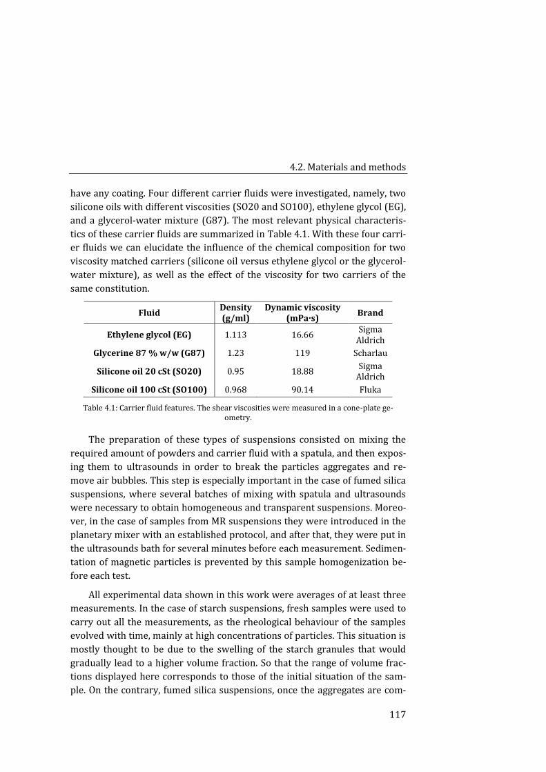
4.2. Materials and methods
117
have any coating. Four different carrier fluids were investigated, namely, two
silicone oils with different viscosities (SO20 and SO100), ethylene glycol (EG),
and a glycerol-water mixture (G87). The most relevant physical characteris-
tics of these carrier fluids are summarized in Table 4.1. With these four carri-
er fluids we can elucidate the influence of the chemical composition for two
viscosity matched carriers (silicone oil versus ethylene glycol or the glycerol-
water mixture), as well as the effect of the viscosity for two carriers of the
same constitution.
Fluid Density (g/ml)
Dynamic viscosity (mPa·s)
Brand
Ethylene glycol (EG) 1.113 16.66 Sigma
Aldrich
Glycerine 87 % w/w (G87) 1.23 119 Scharlau
Silicone oil 20 cSt (SO20) 0.95 18.88 Sigma
Aldrich
Silicone oil 100 cSt (SO100) 0.968 90.14 Fluka
Table 4.1: Carrier fluid features. The shear viscosities were measured in a cone-plate ge-ometry.
The preparation of these types of suspensions consisted on mixing the
required amount of powders and carrier fluid with a spatula, and then expos-
ing them to ultrasounds in order to break the particles aggregates and re-
move air bubbles. This step is especially important in the case of fumed silica
suspensions, where several batches of mixing with spatula and ultrasounds
were necessary to obtain homogeneous and transparent suspensions. Moreo-
ver, in the case of samples from MR suspensions they were introduced in the
planetary mixer with an established protocol, and after that, they were put in
the ultrasounds bath for several minutes before each measurement. Sedimen-
tation of magnetic particles is prevented by this sample homogenization be-
fore each test.
All experimental data shown in this work were averages of at least three
measurements. In the case of starch suspensions, fresh samples were used to
carry out all the measurements, as the rheological behaviour of the samples
evolved with time, mainly at high concentrations of particles. This situation is
mostly thought to be due to the swelling of the starch granules that would
gradually lead to a higher volume fraction. So that the range of volume frac-
tions displayed here corresponds to those of the initial situation of the sam-
ple. On the contrary, fumed silica suspensions, once the aggregates are com-
4. Shear thickening in unimodal suspensions
118
pletely dissolved, are more stable in time. We carried out these measure-
ments the day after the sample preparation. MR suspensions presented a
much better stability, and their rheological behaviour does not change among
measurements carried out in different days if a previous and a correct ho-
mogenization process is followed.
Rheometry 4.2.2.
All rheological tests were carried out in a MCR501 stress-controlled rheome-
ter from Anton Paar at 25 ºC.
For conventional ST suspensions, i.e., those with cornstarch and fumed
silica particles, the geometry used was cone-plate (20 mm diameter, 2º angle,
truncation 0.084 mm). The use of this geometry provides a straightforward
conversion from torque and rotational speed into shear stress and shear rate.
Moreover, it allows to obtain the first normal stress difference (𝑁1 = 𝜎𝑥𝑥 −
𝜎𝑦𝑦) from the normal force acting on the cone (𝑁1 = 2𝐹𝑁/𝜋𝑅2). The protocol
used in these measurements consisted of four steps. The sample was initially
subjected to a preshear at a shear rate of �̇� = 1 s−1 to homogenize it. After
that, rest is imposed by setting a null shear rate and so the normal force. It
helps the sample not to develop normal stresses, by this manner ensuring the
sample to be isotropic at the start of the last step. It consisted in applying a
logarithmic increase in the torque value from 10−4 to 102 mNm. Normal force
data is also registered during this step.
In the case of the carbonyl iron based ST suspensions, the parallel-plate
configuration was used (20 mm diameter, 0.3 mm gap). As a consequence,
raw data from the rheometer was converted into shear rates and stresses by
means of the Weissenberg-Rabinowitch correction, previously explained in
Subsection 3.2.1. The sample volume employed in these tests was 110 µL. The
magnetic field was generated with the aid of an external coil that is capable to
apply uniform magnetic fields up to 15 mT. The protocol was as follows: first,
the sample was loaded onto the geometry. Next, the magnetic field was sud-
denly applied and the sample was left at rest during 60 s. Then, a logarithmic
ramp in shear stress was applied from 0.1 to 10 kPa.
Wall slip corrections were performed for MR samples, as described in
Subsection 3.2.1, although this phenomenon mainly affected the rheological
behaviour of these samples at low shear rates, and few changes appeared at
high shear rates, where the shear thickening may occur.
4.3. Results and discussion
119
Results and discussion 4.3.
In this section the shear-thickening response of two model suspensions is an-
alysed, as a first insight into this phenomenon. Then, we study this behaviour
in concentrated MR fluids, the effect of the composition of the suspending flu-
id and the magnetic field strength.
Starch and fumed silica-based suspensions 4.3.1.
The rheological behaviour of a suspension displaying shear thickening is dis-
played in Figure 1.1. In the typical case [1], an initial plateau is found when
the particles are in equilibrium and can randomly collide and move at low
shear rate or stress. Instead of finding this initial plateau it is possible to have
high viscosity at low shear conditions if interparticle attractions are strong,
what may indicate a yield stress. Then, we observe a shear-thinning region in
which the viscosity of the suspension diminishes as a consequence of the
alignment of particles with the flow. This zone is followed by a Newtonian
plateau with a nearly constant viscosity. A critical point marks the transition
from the Newtonian to the shear-thickening behaviour. It depends on volume
fraction in the case of the critical shear rate but not in the related critical
shear stress. The increase in viscosity at high shear rate or stress can be mild
or more abrupt depending on the volume fraction. In this zone the hydrody-
namic contribution leads to the formation of transient particle aggregates
(hydroclusters) that prevails at moderate concentrations, while the contribu-
tion of contact friction to the shear thickening is more relevant at high volume
fractions. Once the system has reached its maximum value of viscosity, a
Newtonian plateau or a second shear-thinning region is found.
Effect of concentration, particle size and roughness
Shear viscosity as a function of the shear stress for starch and fumed silica
suspensions at several volume fractions is shown in Figure 4.1. The viscosity
curves of these model suspensions slightly vary. At low shear rates, starch
suspensions show an intense shear-thinning region while in the case of fumed
silica the decrease in viscosity is much more moderate and a near Newtonian
behaviour is observed within a great interval of shear stresses.
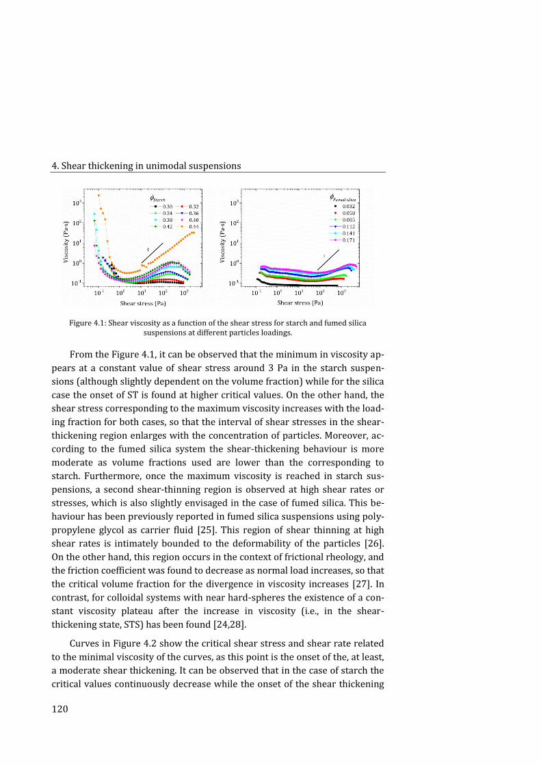
4. Shear thickening in unimodal suspensions
120
Figure 4.1: Shear viscosity as a function of the shear stress for starch and fumed silica suspensions at different particles loadings.
From the Figure 4.1, it can be observed that the minimum in viscosity ap-
pears at a constant value of shear stress around 3 Pa in the starch suspen-
sions (although slightly dependent on the volume fraction) while for the silica
case the onset of ST is found at higher critical values. On the other hand, the
shear stress corresponding to the maximum viscosity increases with the load-
ing fraction for both cases, so that the interval of shear stresses in the shear-
thickening region enlarges with the concentration of particles. Moreover, ac-
cording to the fumed silica system the shear-thickening behaviour is more
moderate as volume fractions used are lower than the corresponding to
starch. Furthermore, once the maximum viscosity is reached in starch sus-
pensions, a second shear-thinning region is observed at high shear rates or
stresses, which is also slightly envisaged in the case of fumed silica. This be-
haviour has been previously reported in fumed silica suspensions using poly-
propylene glycol as carrier fluid [25]. This region of shear thinning at high
shear rates is intimately bounded to the deformability of the particles [26].
On the other hand, this region occurs in the context of frictional rheology, and
the friction coefficient was found to decrease as normal load increases, so that
the critical volume fraction for the divergence in viscosity increases [27]. In
contrast, for colloidal systems with near hard-spheres the existence of a con-
stant viscosity plateau after the increase in viscosity (i.e., in the shear-
thickening state, STS) has been found [24,28].
Curves in Figure 4.2 show the critical shear stress and shear rate related
to the minimal viscosity of the curves, as this point is the onset of the, at least,
a moderate shear thickening. It can be observed that in the case of starch the
critical values continuously decrease while the onset of the shear thickening
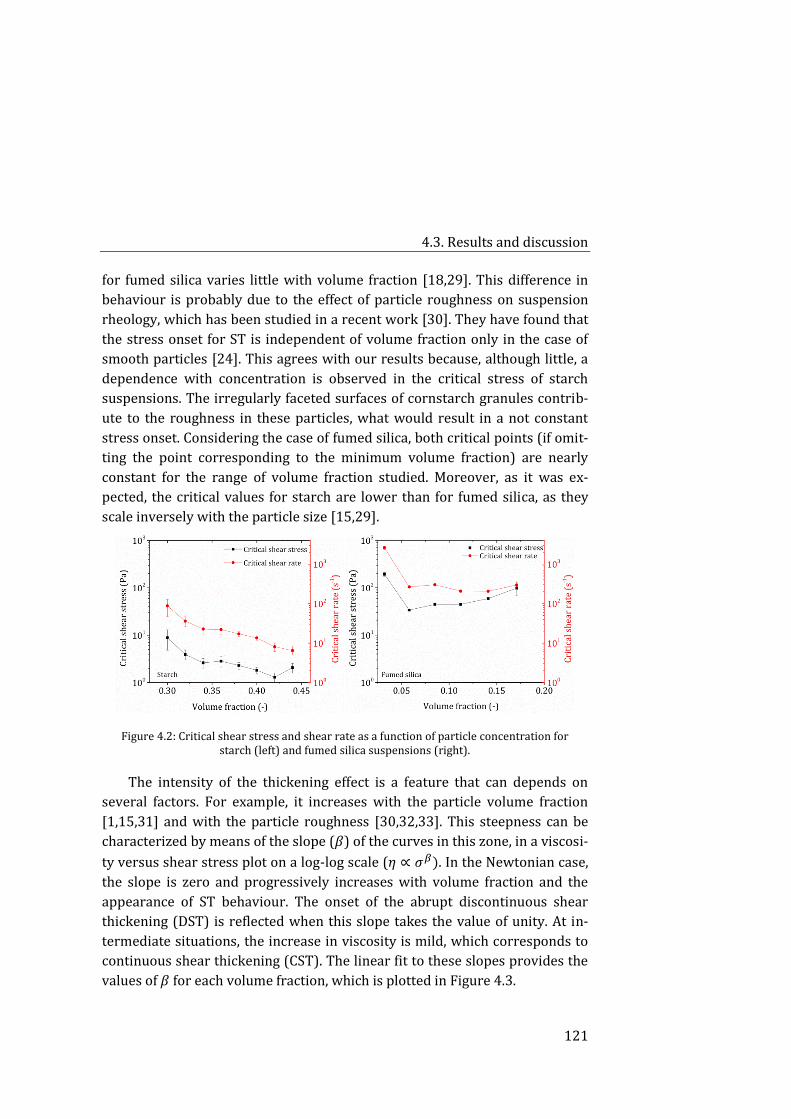
4.3. Results and discussion
121
for fumed silica varies little with volume fraction [18,29]. This difference in
behaviour is probably due to the effect of particle roughness on suspension
rheology, which has been studied in a recent work [30]. They have found that
the stress onset for ST is independent of volume fraction only in the case of
smooth particles [24]. This agrees with our results because, although little, a
dependence with concentration is observed in the critical stress of starch
suspensions. The irregularly faceted surfaces of cornstarch granules contrib-
ute to the roughness in these particles, what would result in a not constant
stress onset. Considering the case of fumed silica, both critical points (if omit-
ting the point corresponding to the minimum volume fraction) are nearly
constant for the range of volume fraction studied. Moreover, as it was ex-
pected, the critical values for starch are lower than for fumed silica, as they
scale inversely with the particle size [15,29].
Figure 4.2: Critical shear stress and shear rate as a function of particle concentration for starch (left) and fumed silica suspensions (right).
The intensity of the thickening effect is a feature that can depends on
several factors. For example, it increases with the particle volume fraction
[1,15,31] and with the particle roughness [30,32,33]. This steepness can be
characterized by means of the slope (𝛽) of the curves in this zone, in a viscosi-
ty versus shear stress plot on a log-log scale (휂 ∝ 𝜎𝛽). In the Newtonian case,
the slope is zero and progressively increases with volume fraction and the
appearance of ST behaviour. The onset of the abrupt discontinuous shear
thickening (DST) is reflected when this slope takes the value of unity. At in-
termediate situations, the increase in viscosity is mild, which corresponds to
continuous shear thickening (CST). The linear fit to these slopes provides the
values of 𝛽 for each volume fraction, which is plotted in Figure 4.3.
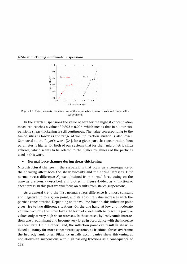
4. Shear thickening in unimodal suspensions
122
Figure 4.3: Beta parameter as a function of the volume fraction for starch and fumed silica suspensions.
In the starch suspensions the value of beta for the highest concentration
measured reaches a value of 0.802 ± 0.006, which means that in all our sus-
pensions shear thickening is still continuous. The value corresponding to the
fumed silica is lower as the range of volume fraction studied is also lower.
Compared to the Royer’s work [24], for a given particle concentration, beta
parameter is higher for both of our systems that for their micrometric silica
spheres, which seems to be related to the higher roughness of the particles
used in this work.
Normal force changes during shear-thickening
Microstructural changes in the suspensions that occur as a consequence of
the shearing affect both the shear viscosity and the normal stresses. First
normal stress difference 𝑁1 was obtained from normal force acting on the
cone as previously described, and plotted in Figure 4.4-left as a function of
shear stress. In this part we will focus on results from starch suspensions.
As a general trend the first normal stress difference is almost constant
and negative up to a given point, and its absolute value increases with the
particle concentration. Depending on the volume fraction, this inflection point
gives rise to two different situations. On the one hand, at low and moderate
volume fractions, the curve takes the form of a well, with 𝑁1 reaching positive
values only at very high shear stresses. In these cases, hydrodynamic interac-
tions are predominant and become very large in accordance with the increase
in shear rate. On the other hand, the inflection point can result in shear in-
duced dilatancy for more concentrated systems, as frictional forces overcome
the hydrodynamic ones. Dilatancy usually accompanies shear thickening at
non-Brownian suspensions with high packing fractions as a consequence of
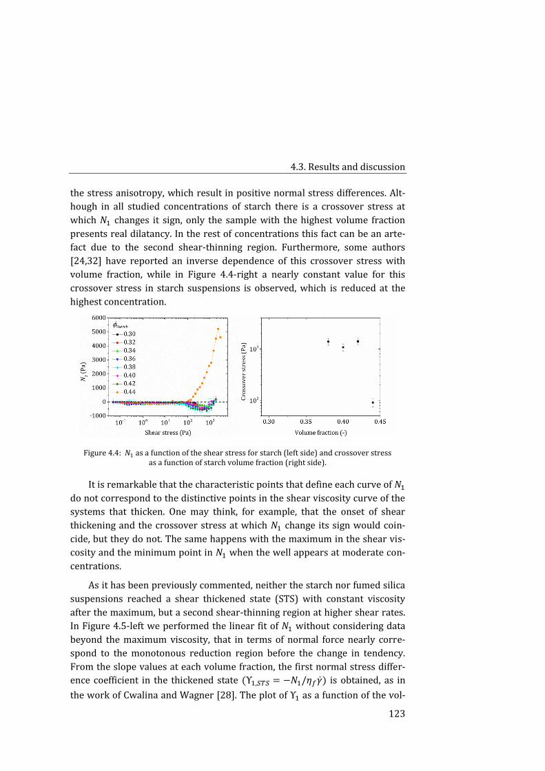
4.3. Results and discussion
123
the stress anisotropy, which result in positive normal stress differences. Alt-
hough in all studied concentrations of starch there is a crossover stress at
which 𝑁1 changes it sign, only the sample with the highest volume fraction
presents real dilatancy. In the rest of concentrations this fact can be an arte-
fact due to the second shear-thinning region. Furthermore, some authors
[24,32] have reported an inverse dependence of this crossover stress with
volume fraction, while in Figure 4.4-right a nearly constant value for this
crossover stress in starch suspensions is observed, which is reduced at the
highest concentration.
Figure 4.4: 𝑁1 as a function of the shear stress for starch (left side) and crossover stress as a function of starch volume fraction (right side).
It is remarkable that the characteristic points that define each curve of 𝑁1
do not correspond to the distinctive points in the shear viscosity curve of the
systems that thicken. One may think, for example, that the onset of shear
thickening and the crossover stress at which 𝑁1 change its sign would coin-
cide, but they do not. The same happens with the maximum in the shear vis-
cosity and the minimum point in 𝑁1 when the well appears at moderate con-
centrations.
As it has been previously commented, neither the starch nor fumed silica
suspensions reached a shear thickened state (STS) with constant viscosity
after the maximum, but a second shear-thinning region at higher shear rates.
In Figure 4.5-left we performed the linear fit of 𝑁1 without considering data
beyond the maximum viscosity, that in terms of normal force nearly corre-
spond to the monotonous reduction region before the change in tendency.
From the slope values at each volume fraction, the first normal stress differ-
ence coefficient in the thickened state (Υ1,𝑆𝑇𝑆 = −𝑁1/휂𝑓�̇�) is obtained, as in
the work of Cwalina and Wagner [28]. The plot of Υ1 as a function of the vol-
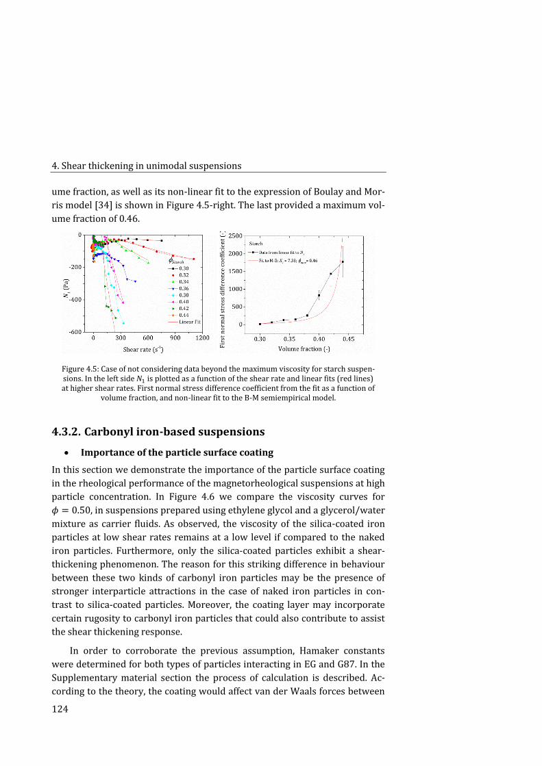
4. Shear thickening in unimodal suspensions
124
ume fraction, as well as its non-linear fit to the expression of Boulay and Mor-
ris model [34] is shown in Figure 4.5-right. The last provided a maximum vol-
ume fraction of 0.46.
Figure 4.5: Case of not considering data beyond the maximum viscosity for starch suspen-sions. In the left side 𝑁1 is plotted as a function of the shear rate and linear fits (red lines) at higher shear rates. First normal stress difference coefficient from the fit as a function of
volume fraction, and non-linear fit to the B-M semiempirical model.
Carbonyl iron-based suspensions 4.3.2.
Importance of the particle surface coating
In this section we demonstrate the importance of the particle surface coating
in the rheological performance of the magnetorheological suspensions at high
particle concentration. In Figure 4.6 we compare the viscosity curves for
𝜙 = 0.50, in suspensions prepared using ethylene glycol and a glycerol/water
mixture as carrier fluids. As observed, the viscosity of the silica-coated iron
particles at low shear rates remains at a low level if compared to the naked
iron particles. Furthermore, only the silica-coated particles exhibit a shear-
thickening phenomenon. The reason for this striking difference in behaviour
between these two kinds of carbonyl iron particles may be the presence of
stronger interparticle attractions in the case of naked iron particles in con-
trast to silica-coated particles. Moreover, the coating layer may incorporate
certain rugosity to carbonyl iron particles that could also contribute to assist
the shear thickening response.
In order to corroborate the previous assumption, Hamaker constants
were determined for both types of particles interacting in EG and G87. In the
Supplementary material section the process of calculation is described. Ac-
cording to the theory, the coating would affect van der Waals forces between
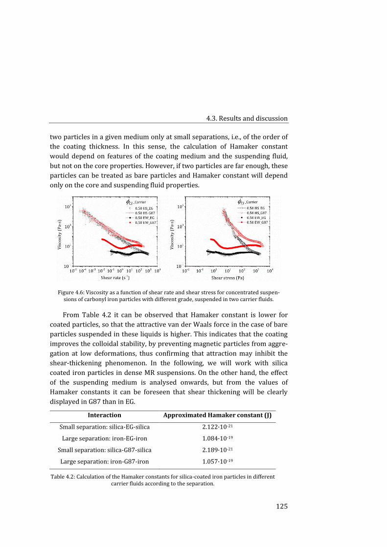
4.3. Results and discussion
125
two particles in a given medium only at small separations, i.e., of the order of
the coating thickness. In this sense, the calculation of Hamaker constant
would depend on features of the coating medium and the suspending fluid,
but not on the core properties. However, if two particles are far enough, these
particles can be treated as bare particles and Hamaker constant will depend
only on the core and suspending fluid properties.
Figure 4.6: Viscosity as a function of shear rate and shear stress for concentrated suspen-sions of carbonyl iron particles with different grade, suspended in two carrier fluids.
From Table 4.2 it can be observed that Hamaker constant is lower for
coated particles, so that the attractive van der Waals force in the case of bare
particles suspended in these liquids is higher. This indicates that the coating
improves the colloidal stability, by preventing magnetic particles from aggre-
gation at low deformations, thus confirming that attraction may inhibit the
shear-thickening phenomenon. In the following, we will work with silica
coated iron particles in dense MR suspensions. On the other hand, the effect
of the suspending medium is analysed onwards, but from the values of
Hamaker constants it can be foreseen that shear thickening will be clearly
displayed in G87 than in EG.
Interaction Approximated Hamaker constant (J)
Small separation: silica-EG-silica 2.122·10-21
Large separation: iron-EG-iron 1.084·10-19
Small separation: silica-G87-silica 2.189·10-21
Large separation: iron-G87-iron 1.057·10-19
Table 4.2: Calculation of the Hamaker constants for silica-coated iron particles in different carrier fluids according to the separation.
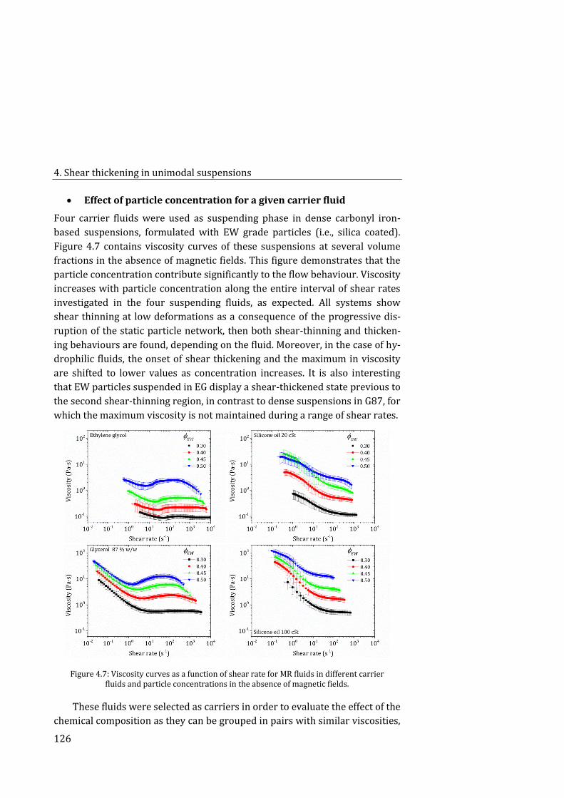
4. Shear thickening in unimodal suspensions
126
Effect of particle concentration for a given carrier fluid
Four carrier fluids were used as suspending phase in dense carbonyl iron-
based suspensions, formulated with EW grade particles (i.e., silica coated).
Figure 4.7 contains viscosity curves of these suspensions at several volume
fractions in the absence of magnetic fields. This figure demonstrates that the
particle concentration contribute significantly to the flow behaviour. Viscosity
increases with particle concentration along the entire interval of shear rates
investigated in the four suspending fluids, as expected. All systems show
shear thinning at low deformations as a consequence of the progressive dis-
ruption of the static particle network, then both shear-thinning and thicken-
ing behaviours are found, depending on the fluid. Moreover, in the case of hy-
drophilic fluids, the onset of shear thickening and the maximum in viscosity
are shifted to lower values as concentration increases. It is also interesting
that EW particles suspended in EG display a shear-thickened state previous to
the second shear-thinning region, in contrast to dense suspensions in G87, for
which the maximum viscosity is not maintained during a range of shear rates.
Figure 4.7: Viscosity curves as a function of shear rate for MR fluids in different carrier fluids and particle concentrations in the absence of magnetic fields.
These fluids were selected as carriers in order to evaluate the effect of the
chemical composition as they can be grouped in pairs with similar viscosities,
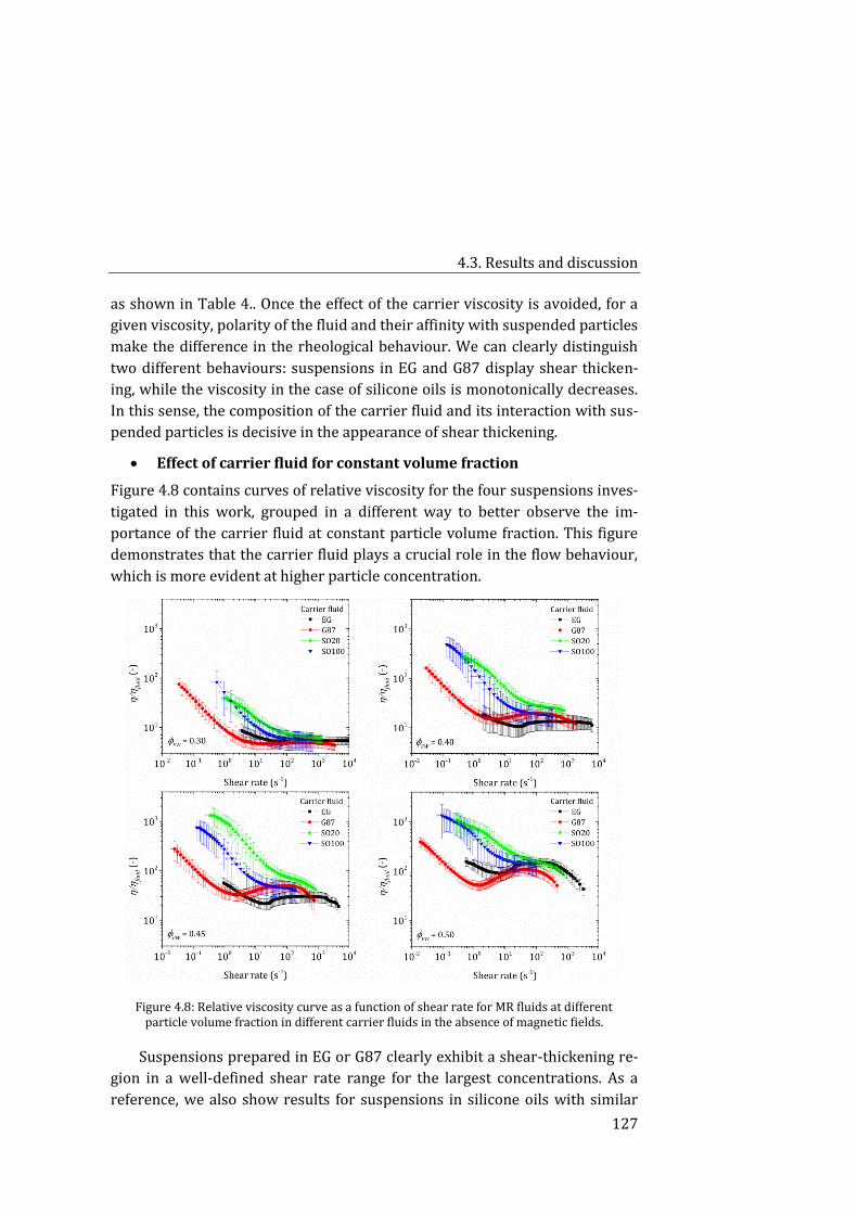
4.3. Results and discussion
127
as shown in Table 4.. Once the effect of the carrier viscosity is avoided, for a
given viscosity, polarity of the fluid and their affinity with suspended particles
make the difference in the rheological behaviour. We can clearly distinguish
two different behaviours: suspensions in EG and G87 display shear thicken-
ing, while the viscosity in the case of silicone oils is monotonically decreases.
In this sense, the composition of the carrier fluid and its interaction with sus-
pended particles is decisive in the appearance of shear thickening.
Effect of carrier fluid for constant volume fraction
Figure 4.8 contains curves of relative viscosity for the four suspensions inves-
tigated in this work, grouped in a different way to better observe the im-
portance of the carrier fluid at constant particle volume fraction. This figure
demonstrates that the carrier fluid plays a crucial role in the flow behaviour,
which is more evident at higher particle concentration.
Figure 4.8: Relative viscosity curve as a function of shear rate for MR fluids at different particle volume fraction in different carrier fluids in the absence of magnetic fields.
Suspensions prepared in EG or G87 clearly exhibit a shear-thickening re-
gion in a well-defined shear rate range for the largest concentrations. As a
reference, we also show results for suspensions in silicone oils with similar
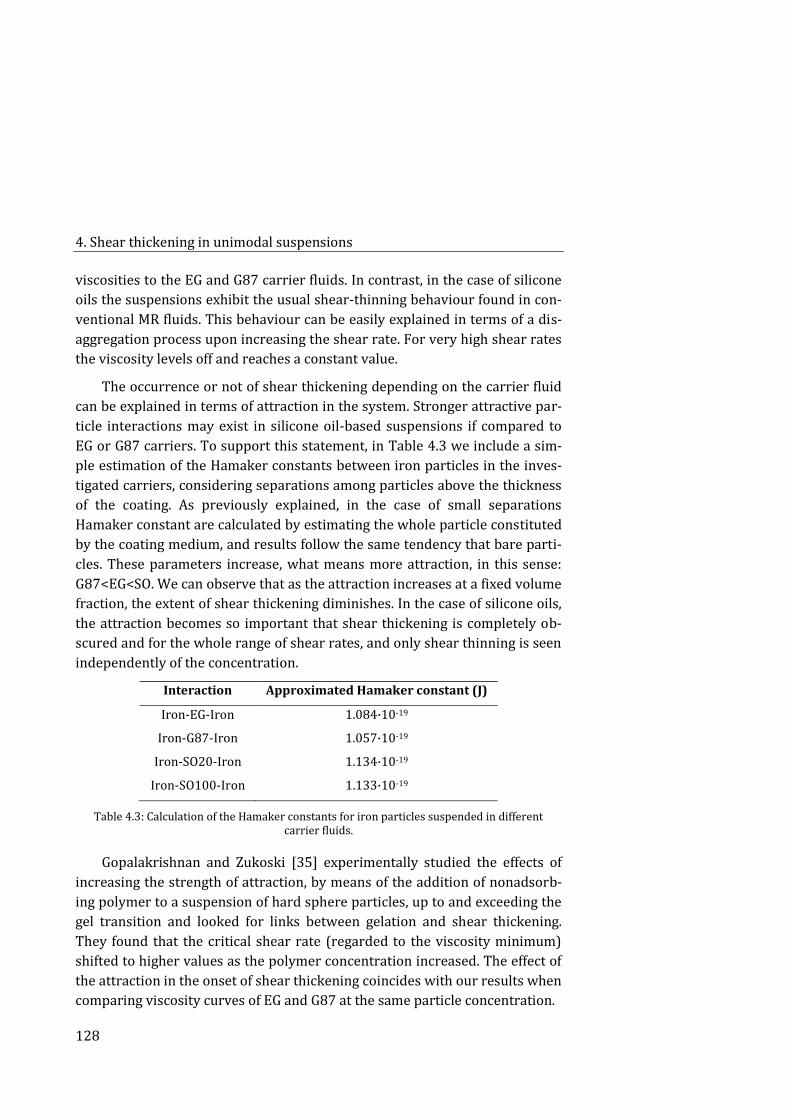
4. Shear thickening in unimodal suspensions
128
viscosities to the EG and G87 carrier fluids. In contrast, in the case of silicone
oils the suspensions exhibit the usual shear-thinning behaviour found in con-
ventional MR fluids. This behaviour can be easily explained in terms of a dis-
aggregation process upon increasing the shear rate. For very high shear rates
the viscosity levels off and reaches a constant value.
The occurrence or not of shear thickening depending on the carrier fluid
can be explained in terms of attraction in the system. Stronger attractive par-
ticle interactions may exist in silicone oil-based suspensions if compared to
EG or G87 carriers. To support this statement, in Table 4.3 we include a sim-
ple estimation of the Hamaker constants between iron particles in the inves-
tigated carriers, considering separations among particles above the thickness
of the coating. As previously explained, in the case of small separations
Hamaker constant are calculated by estimating the whole particle constituted
by the coating medium, and results follow the same tendency that bare parti-
cles. These parameters increase, what means more attraction, in this sense:
G87<EG<SO. We can observe that as the attraction increases at a fixed volume
fraction, the extent of shear thickening diminishes. In the case of silicone oils,
the attraction becomes so important that shear thickening is completely ob-
scured and for the whole range of shear rates, and only shear thinning is seen
independently of the concentration.
Interaction Approximated Hamaker constant (J)
Iron-EG-Iron 1.084·10-19
Iron-G87-Iron 1.057·10-19
Iron-SO20-Iron 1.134·10-19
Iron-SO100-Iron 1.133·10-19
Table 4.3: Calculation of the Hamaker constants for iron particles suspended in different carrier fluids.
Gopalakrishnan and Zukoski [35] experimentally studied the effects of
increasing the strength of attraction, by means of the addition of nonadsorb-
ing polymer to a suspension of hard sphere particles, up to and exceeding the
gel transition and looked for links between gelation and shear thickening.
They found that the critical shear rate (regarded to the viscosity minimum)
shifted to higher values as the polymer concentration increased. The effect of
the attraction in the onset of shear thickening coincides with our results when
comparing viscosity curves of EG and G87 at the same particle concentration.
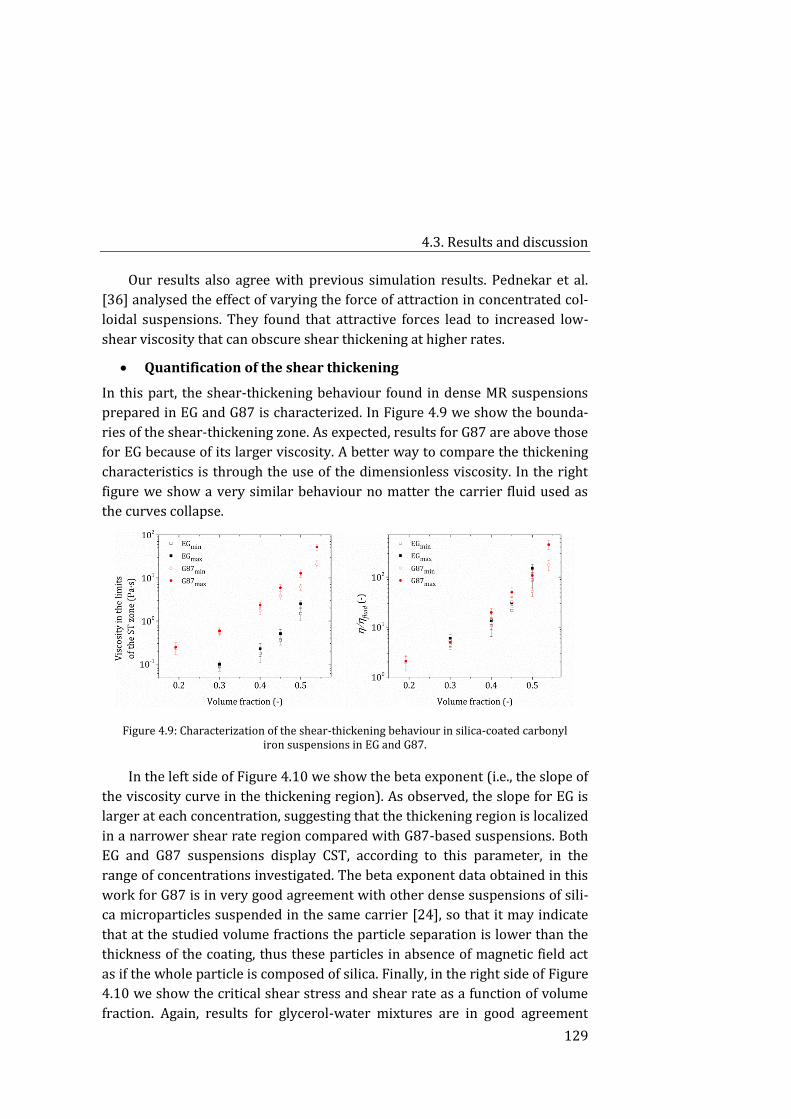
4.3. Results and discussion
129
Our results also agree with previous simulation results. Pednekar et al.
[36] analysed the effect of varying the force of attraction in concentrated col-
loidal suspensions. They found that attractive forces lead to increased low-
shear viscosity that can obscure shear thickening at higher rates.
Quantification of the shear thickening
In this part, the shear-thickening behaviour found in dense MR suspensions
prepared in EG and G87 is characterized. In Figure 4.9 we show the bounda-
ries of the shear-thickening zone. As expected, results for G87 are above those
for EG because of its larger viscosity. A better way to compare the thickening
characteristics is through the use of the dimensionless viscosity. In the right
figure we show a very similar behaviour no matter the carrier fluid used as
the curves collapse.
Figure 4.9: Characterization of the shear-thickening behaviour in silica-coated carbonyl iron suspensions in EG and G87.
In the left side of Figure 4.10 we show the beta exponent (i.e., the slope of
the viscosity curve in the thickening region). As observed, the slope for EG is
larger at each concentration, suggesting that the thickening region is localized
in a narrower shear rate region compared with G87-based suspensions. Both
EG and G87 suspensions display CST, according to this parameter, in the
range of concentrations investigated. The beta exponent data obtained in this
work for G87 is in very good agreement with other dense suspensions of sili-
ca microparticles suspended in the same carrier [24], so that it may indicate
that at the studied volume fractions the particle separation is lower than the
thickness of the coating, thus these particles in absence of magnetic field act
as if the whole particle is composed of silica. Finally, in the right side of Figure
4.10 we show the critical shear stress and shear rate as a function of volume
fraction. Again, results for glycerol-water mixtures are in good agreement
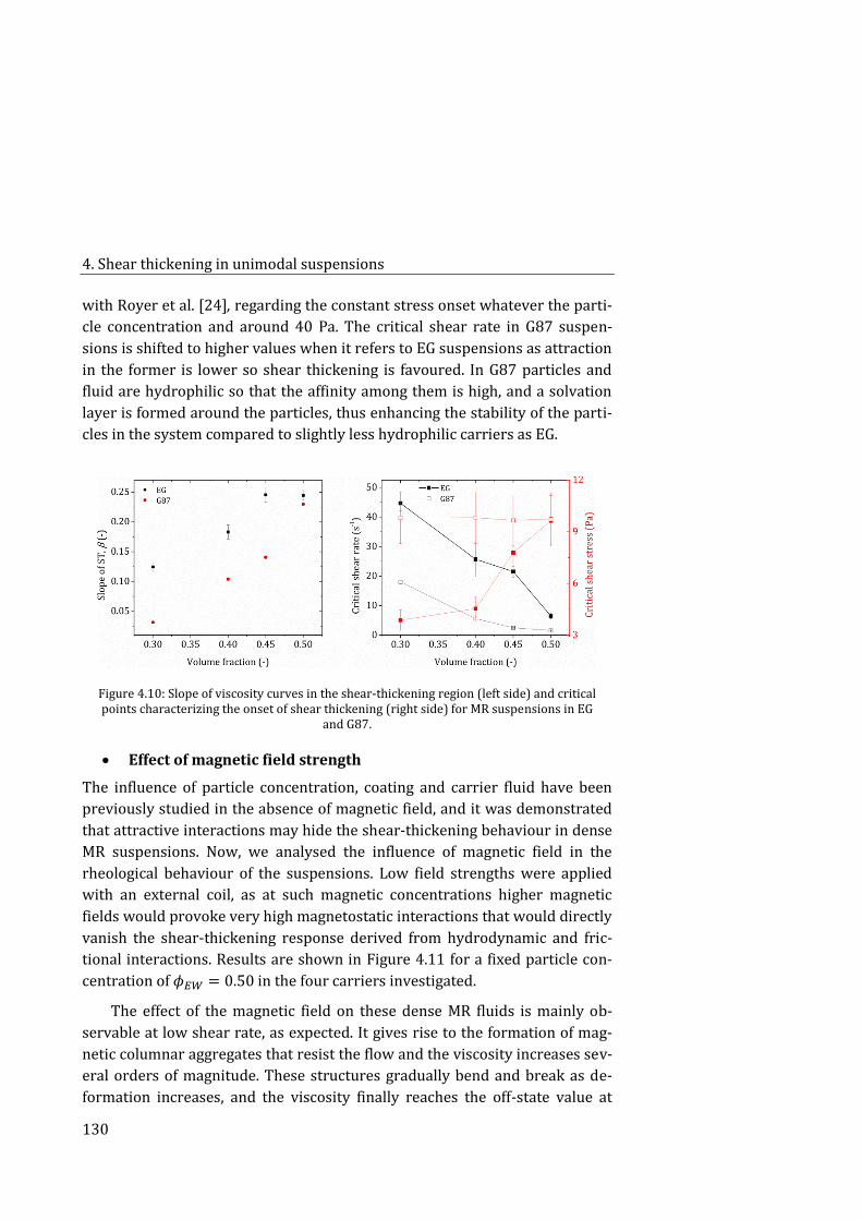
4. Shear thickening in unimodal suspensions
130
with Royer et al. [24], regarding the constant stress onset whatever the parti-
cle concentration and around 40 Pa. The critical shear rate in G87 suspen-
sions is shifted to higher values when it refers to EG suspensions as attraction
in the former is lower so shear thickening is favoured. In G87 particles and
fluid are hydrophilic so that the affinity among them is high, and a solvation
layer is formed around the particles, thus enhancing the stability of the parti-
cles in the system compared to slightly less hydrophilic carriers as EG.
Figure 4.10: Slope of viscosity curves in the shear-thickening region (left side) and critical points characterizing the onset of shear thickening (right side) for MR suspensions in EG
and G87.
Effect of magnetic field strength
The influence of particle concentration, coating and carrier fluid have been
previously studied in the absence of magnetic field, and it was demonstrated
that attractive interactions may hide the shear-thickening behaviour in dense
MR suspensions. Now, we analysed the influence of magnetic field in the
rheological behaviour of the suspensions. Low field strengths were applied
with an external coil, as at such magnetic concentrations higher magnetic
fields would provoke very high magnetostatic interactions that would directly
vanish the shear-thickening response derived from hydrodynamic and fric-
tional interactions. Results are shown in Figure 4.11 for a fixed particle con-
centration of 𝜙𝐸𝑊 = 0.50 in the four carriers investigated.
The effect of the magnetic field on these dense MR fluids is mainly ob-
servable at low shear rate, as expected. It gives rise to the formation of mag-
netic columnar aggregates that resist the flow and the viscosity increases sev-
eral orders of magnitude. These structures gradually bend and break as de-
formation increases, and the viscosity finally reaches the off-state value at
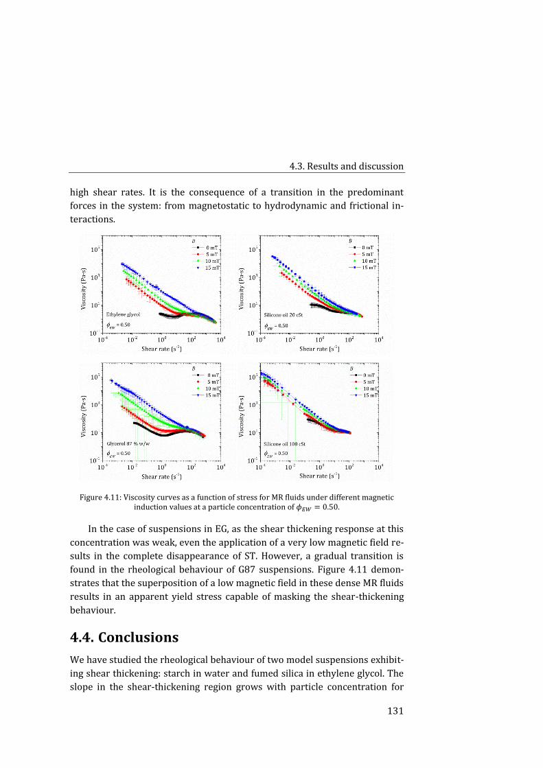
4.3. Results and discussion
131
high shear rates. It is the consequence of a transition in the predominant
forces in the system: from magnetostatic to hydrodynamic and frictional in-
teractions.
Figure 4.11: Viscosity curves as a function of stress for MR fluids under different magnetic induction values at a particle concentration of 𝜙𝐸𝑊 = 0.50.
In the case of suspensions in EG, as the shear thickening response at this
concentration was weak, even the application of a very low magnetic field re-
sults in the complete disappearance of ST. However, a gradual transition is
found in the rheological behaviour of G87 suspensions. Figure 4.11 demon-
strates that the superposition of a low magnetic field in these dense MR fluids
results in an apparent yield stress capable of masking the shear-thickening
behaviour.
Conclusions 4.4.
We have studied the rheological behaviour of two model suspensions exhibit-
ing shear thickening: starch in water and fumed silica in ethylene glycol. The
slope in the shear-thickening region grows with particle concentration for
4. Shear thickening in unimodal suspensions
132
both systems, as expected, but beta is always below the unity, meaning CST in
all the experiments. Differences in the viscous response of starch and fumed
silica suspensions can be explained in terms of particle features, as at very
high concentrations friction between them is the largest contribution. In this
sense, the onset of the shear thickening shifts to lower shear rates in the case
of starch that may be due to a combination of higher friction of irregularly
faceted surfaces of starch granules and a higher particle diameter, compared
to fumed silica aggregates. On the other hand, both systems exhibit a second
shear-thinning region above the shear stress of the maximum viscosity, as a
consequence of the particle deformability. Regarding measurements on nor-
mal force in starch suspensions, negative values of 𝑁1 at low shear rates cor-
respond to a predominant contribution of hydrodynamic forces when the
suspension is subjected to increasing shear rates. In this sense, 𝑁1 scales line-
arly with the shear rate around the shear-thickening zone. On the contrary, at
higher shear rates particles are pushed closer, which causes 𝑁1 to become
positive when frictional interactions overcome those coming from hydrody-
namics. Dilation is observed at shear stresses above the onset stress of shear
thickening. A characteristic well in the 𝑁1 profile appears just before the tran-
sition in 𝑁1 for CST situations but not at volume fractions near DST. At higher
stresses, the analysis of parameters derived from normal force measurement
provides a diverging volume fraction of 0.46.
On the other hand, dense MR fluids were selected for further studying
shear thickening and the possibility of tuning this response. It is demonstrat-
ed that the chemical properties of particles and suspending fluids affect the
appearance of shear thickening in dense suspensions. In this way, carbonyl
iron particles with different grades display different rheological behaviours.
Indeed, dense suspensions of carbonyl iron particles EW in silicone oil display
shear thinning in the whole range of shear rates, while those formulated in EG
and G87 provide shear-thickening behaviour. In this sense, a higher affinity
between particles and carrier, reflected in Hamaker constant values, pro-
motes the formation of a solvation layer that could reduce the attraction be-
tween particles, thus enhancing shear thickening. Finally, when magnetic field
is applied, great magnetostatic interactions dominate the flow behaviour at
low shear rates and progressively inhibit the shear-thickening response in EG
and G87 suspensions.
4.5. Supplementary material
133
Supplementary material 4.5.
Van der Waals interactions
Electrostatic repulsion together with Van der Waals interactions (attractive)
are the main contributions to the colloidal stability of a suspension, according
to the DLVO theory. Thus, the simplest way to minimize interactions between
colloidal particles is by means of reducing the van der Waals attraction. In the
common situation involving two spheres or macromolecules of radii 𝑅1 and
𝑅2, Van der Waals interaction energy 𝑊 and force 𝐹 are given by [37]:
𝑊 = −𝐴
6𝐷(
𝑅1𝑅2
𝑅1 + 𝑅2) , 𝐹 = −
𝐴
6𝐷2(
𝑅1𝑅2
𝑅1 + 𝑅2), (4.1)
being 𝐴 the Hamaker constant, and 𝐷 the separation between the surfaces of
the particles.
Hamaker constants calculation
In the particular case of two identical phases (1 and 2) interacting across me-
dium 3, the Hamaker constant can be written as:
𝐴 = 𝐴131 ≈3
4𝑘𝑇 (
휀1 − 휀3
휀1 + 휀3)
2
+3ℎ𝜈𝑒
16√2
(𝑛12 − 𝑛3
2)2
(𝑛12 + 𝑛3
2) 3/2 , (4.2)
where ℎ = 6.626 · 10−34 J/s is the Planck’s constant, 𝑘 = 1.381 · 10−34 J/K is
the Boltzmann’s constant, 𝜈𝑒 is the absorption frequency, 휀 the medium
permittivity, 𝑛 the refractive index, and 𝑇 the temperature. In the absence of
the real values of the absorption frequency for each component, we used
𝜈𝑒 = 1015 s−1 as a typical value from literature [37]. This parameter was as-
sumed as constant for the three media involved in the calculation of the ap-
proximated Hamaker constants. The form of the equation indicates that 𝐴 is
always positive, so that Van der Waals force is always attractive.
In order to estimate the Hamaker constant we need to know the values of
permittivity and refractive index of all the components of the suspensions.
Refractive indices of carrier fluids were experimentally measured, and the
rest of data were gathered from literature. In the absence of neither of these
parameters for carbonyl iron particles, 휀 and 𝑛 of iron were used instead in
the calculation of the VdW interactions. They are listed in Table 4.4.
In the case of particles (medium 1) coated by an adsorbed layer (medium
2) with thickness 𝑇, the Hamaker constant used in van der Waals interaction
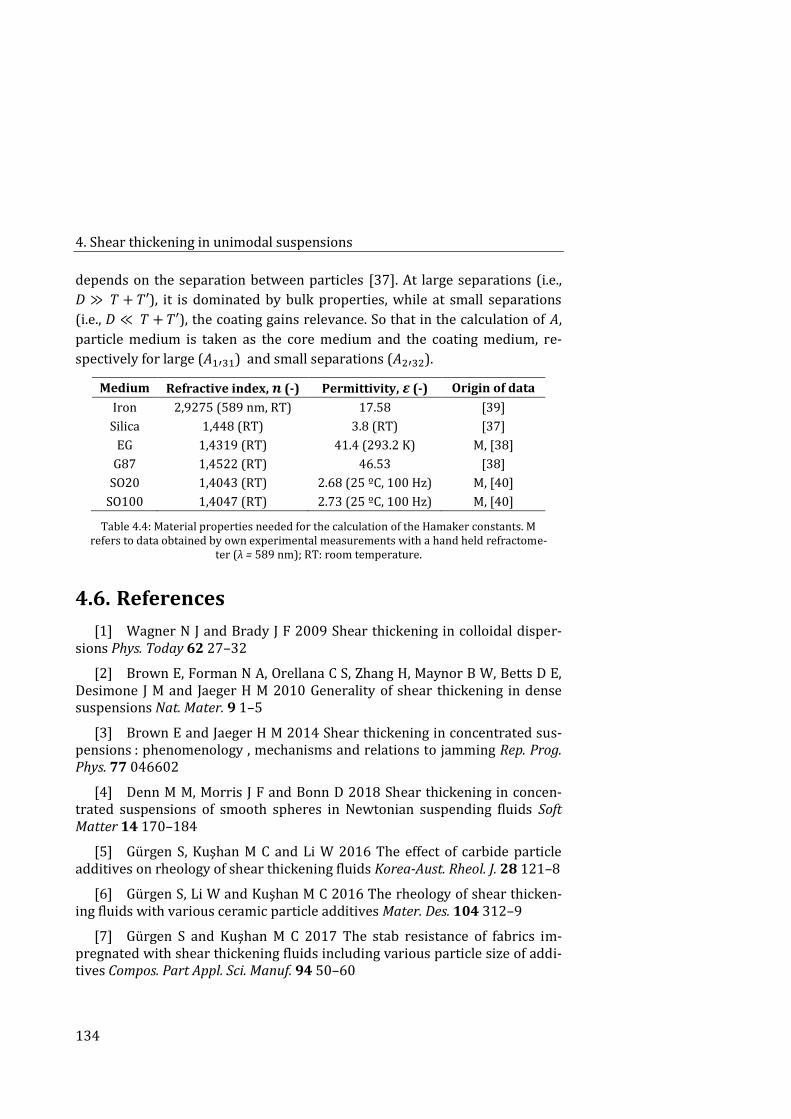
4. Shear thickening in unimodal suspensions
134
depends on the separation between particles [37]. At large separations (i.e.,
𝐷 ≫ 𝑇 + 𝑇′), it is dominated by bulk properties, while at small separations
(i.e., 𝐷 ≪ 𝑇 + 𝑇′), the coating gains relevance. So that in the calculation of 𝐴,
particle medium is taken as the core medium and the coating medium, re-
spectively for large (𝐴1′31) and small separations (𝐴2′32).
Medium Refractive index, 𝒏 (-) Permittivity, 𝜺 (-) Origin of data
Iron 2,9275 (589 nm, RT) 17.58 [39]
Silica 1,448 (RT) 3.8 (RT) [37]
EG 1,4319 (RT) 41.4 (293.2 K) M, [38]
G87 1,4522 (RT) 46.53 [38]
SO20 1,4043 (RT) 2.68 (25 ºC, 100 Hz) M, [40]
SO100 1,4047 (RT) 2.73 (25 ºC, 100 Hz) M, [40]
Table 4.4: Material properties needed for the calculation of the Hamaker constants. M refers to data obtained by own experimental measurements with a hand held refractome-
ter (λ = 589 nm); RT: room temperature.
References 4.6.
[1] Wagner N J and Brady J F 2009 Shear thickening in colloidal disper-sions Phys. Today 62 27–32
[2] Brown E, Forman N A, Orellana C S, Zhang H, Maynor B W, Betts D E, Desimone J M and Jaeger H M 2010 Generality of shear thickening in dense suspensions Nat. Mater. 9 1–5
[3] Brown E and Jaeger H M 2014 Shear thickening in concentrated sus-pensions : phenomenology , mechanisms and relations to jamming Rep. Prog. Phys. 77 046602
[4] Denn M M, Morris J F and Bonn D 2018 Shear thickening in concen-trated suspensions of smooth spheres in Newtonian suspending fluids Soft Matter 14 170–184
[5] Gürgen S, Kuşhan M C and Li W 2016 The effect of carbide particle additives on rheology of shear thickening fluids Korea-Aust. Rheol. J. 28 121–8
[6] Gürgen S, Li W and Kuşhan M C 2016 The rheology of shear thicken-ing fluids with various ceramic particle additives Mater. Des. 104 312–9
[7] Gürgen S and Kuşhan M C 2017 The stab resistance of fabrics im-pregnated with shear thickening fluids including various particle size of addi-tives Compos. Part Appl. Sci. Manuf. 94 50–60
4.6. References
135
[8] Li D, Wang R, Liu X, Fang S and Sun Y 2018 Shear-thickening fluid us-ing oxygen-plasma-modified multi-walled carbon nanotubes to improve the quasi-static stab resistance of Kevlar fabrics Polymers 10 1356
[9] Gürgen S, Sofuoğlu M A and Kuşhan M C 2019 Rheological compatibil-ity of multi-phase shear thickening fluid with a phenomenological model Smart Mater. Struct. 28 035027
[10] Zhang X, Li W and Gong X L 2008 Study on magnetorheological shear thickening fluid Smart Mater. Struct. 17 015051
[11] Peng G R, Li W, Tian T F, Ding J and Nakano M 2014 Experimental and modeling study of viscoelastic behaviors of magneto-rheological shear thick-ening fluids Korea-Aust. Rheol. J. 26 149–158
[12] Bossis G, Grasselli Y, Meunier A and Volkova O 2016 Outstanding magnetorheological effect based on discontinuous shear thickening in the presence of a superplastifier molecule Appl. Phys. Lett. 109 111902
[13] Galindo-Rosales F 2016 Complex fluids in energy dissipating systems Appl. Sci. 6 206
[14] Metzner A B and Whitlock M 1958 Flow behavior of concentrated (di-latant) suspensions Trans. Soc. Rheol. 2 239–54
[15] Barnes H A 1989 Shear-thickening (“Dilatancy”) in suspensions of nonaggregating solid particles dispersed in Newtonian liquids J. Rheol. 33 329–366
[16] Hoffman R L 1974 Discontinuous and dilatant viscosity behavior in concentrated suspensions. II. Theory and experimental tests J. Colloid Inter-face Sci. 46 491–506
[17] Brady J F and Bossis G 1985 The rheology of concentrated suspen-sions of spheres in simple shear flow by numerical simulation J. Fluid Mech. 155 105
[18] Brown E and Jaeger H M 2012 The role of dilation and confining stresses in shear thickening of dense suspensions J. Rheol. 56 875–923
[19] Seto R, Mari R, Morris J F and Denn M M 2013 Discontinuous shear thickening of frictional hard-sphere suspensions Phys. Rev. Lett. 111 1–5
[20] Fernandez N, Mani R, Rinaldi D, Kadau D, Mosquet M, Lombois-Burger H, Cayer-Barrioz J, Herrmann H J, Spencer N D and Isa L 2013 Micro-scopic mechanism for shear thickening of non-brownian suspensions Phys. Rev. Lett. 111 1–5
[21] Mari R, Seto R, Morris J F and Denn M M 2014 Shear thickening, fric-tionless and frictional rheologies in non-Brownian suspensions J. Rheol. 58 32
4. Shear thickening in unimodal suspensions
136
[22] Singh A, Mari R, Denn M M and Morris J F 2018 A constitutive model for simple shear of dense frictional suspensions J. Rheol. 62 457–68
[23] Lin N Y C, Guy B M, Hermes M, Ness C, Sun J, Poon W C K and Cohen I 2015 Hydrodynamic and contact contributions to continuous shear thicken-ing in colloidal suspensions Phys. Rev. Lett. 115
[24] Royer J R, Blair D L and Hudson S D 2016 Rheological signature of frictional interactions in shear thickening suspensions Phys. Rev. Lett. 116
[25] Raghavan S R and Khan S A 1997 Shear-thickening response of fumed silica suspensions under steady and oscillatory shear J. Colloid Interface Sci. 185 57–67
[26] Kalman D P, Rosen B A, Wagner N J, Co A, Leal G L, Colby R H and Giacomin A J 2008 Effects of Particle Hardness on Shear Thickening Colloidal Suspension Rheology AIP Conference Proceedings (AIP)
[27] Chatté G, Comtet J, Niguès A, Bocquet L, Siria A, Ducouret G, Lequeux F, Lenoir N, Ovarlez G and Colin A 2018 Shear thinning in non-Brownian sus-pensions Soft Matter 14 879–893
[28] Cwalina C D and Wagner N J 2014 Material properties of the shear-thickened state in concentrated near hard-sphere colloidal dispersions J. Rhe-ol. 58 949–67
[29] Maranzano B J and Wagner N J 2001 The effects of particle size on re-versible shear thickening of concentrated colloidal dispersions J. Chem. Phys. 114 10514
[30] Hsiao L C, Jamali S, Glynos E, Green P F, Larson R G and Solomon M J 2017 Rheological state diagrams for rough colloids in shear flow Phys. Rev. Lett. 119
[31] Brown E and Jaeger H M 2009 Dynamic jamming point for shear thickening suspensions Phys. Rev. Lett. 103
[32] Lootens D, Van Damme H, Hémar Y and Hebraud P 2005 Dilatant flow of concentrated suspensions of rough particles Phys. Rev. Lett. 95 1–4
[33] Hsu C-P, Ramakrishna S N, Zanini M, Spencer N D and Isa L 2018 Roughness-dependent tribology effects on discontinuous shear thickening Proc. Natl. Acad. Sci. 1–6
[34] Morris J F and Boulay F 1999 Curvilinear flows of noncolloidal sus-pensions: The role of normal stresses J. Rheol. 43 1213–1237
[35] Gopalakrishnan V and Zukoski C F 2004 Effect of attractions on shear thickening in dense suspensions J. Rheol. 48 1321–1344
4.6. References
137
[36] Pednekar S, Chun J and Morris J F 2017 Simulation of shear thicken-ing in attractive colloidal suspensions Soft Matter 13 1773–1779
[37] Israelachvili J N 2011 Intermolecular and surface forces (San Diego: Academic Press)
[38] Lide D R 2012 CRC Handbook of Chemistry and Physics (CRC Boca Ra-ton)
[39] M. N. Polyanskiy, "Refractive index database," https://refractiveindex.info. Accessed on 2020-02-13.
[40] Clearco Products Co., Inc., “Dielectric properties of pure silicone flu-ids”, http://www.clearcoproducts.com/pdf/pure-silicone/Dielectric_Proper-ties_Pure_Silicone_Fluids.pdf. Accessed on 2020-02-13.

139
5. Shear thickening in bimodal
suspensions
Introduction 5.1.
Suspension rheology [1–3] is capturing a great interest in recent years due to
the importance of complex suspensions in multitude of industrial applica-
tions. The desired performance of this kind of materials is affected by many
factors that can be classified into those related to the particle properties [4–7]
(e.g., size, form, size distribution, composition, concentration, electrical
charge…), suspending medium (such as viscosity) and flow conditions im-
posed to the suspension.
Unimodal suspensions, i.e., suspensions formulated with a unique type of
particle as suspended phase, are extensively investigated in literature. Among
them, in this thesis special attention is paid to two remarkable types of uni-
modal suspensions for their ability of readily tuning their rheological behav-
iour, well passively by shear or actively by external fields: shear-thickening
(ST) and magnetorheological (MR) fluids, both used in energy dissipating sys-
tems [8]. The formers are used as impact-resistant materials or shock ab-
sorbers in protective applications while MR fluids are very valued materials
in devices for torque transfer, as clutches or dampers.
5. Shear thickening in bimodal suspensions
140
Briefly, the counter-intuitive phenomenon of shear thickening [9,10] dis-
plays a reversible increase in viscosity (continuous or discontinuous) under
applied shear rates or stresses. Despite the complexity of this shear-induced
response due to the substantial amount of particles involved within the sys-
tem, and after several decades of debate about the physical mechanism [11–
15] that originates this response, nowadays scientific community broadly
agrees that ST is due to a transition from a hydrodynamically lubricated re-
gime to a friction dominated situation [16–20]. This non-Newtonian behav-
iour exists above a critical volume fraction and shear rate, in systems where
attraction is negligible. Indeed Barnes [21] reviewed this behaviour and stat-
ed that “given the right circumstances, all suspensions of solid particles will
show the phenomenon”. The possibility of controlling these critical parame-
ters or the severity of the shear thickening poses a great challenge to scien-
tists. In literature we can found several strategies to tune the thickening fea-
tures, such as altering some properties during the formulation [15,22–24]
(e.g., particle or fluid characteristics, like size, shape, polydispersity or rough-
ness) or introducing flow disturbances [25]. In fact, shear thickening can even
be completely obscured by tuning these particle features or destabilizing the
system by introducing net attractive forces [26]. Dense suspensions of corn-
starch in water are the typical model systems that show this dramatic change
in viscosity.
On the other hand, as in the case of ST fluids, the rheological properties of
MR fluids can also be varied. They are suspensions of magnetic micronsized
particles suspended in a non-magnetic Newtonian fluid. When subjected to an
external magnetic field these particles become polarized and aggregate in
chains or columnar structures that orientate along magnetic field lines. As a
result of this field-induced assembly, the suspension experiences a reversible
liquid-to-solid transition as the viscosity of MR fluids rapidly increases sever-
al orders of magnitude, what is known as magnetorheological effect [27]. Un-
der certain external fields and particle volume fractions the increase in flow
resistance may develop a field-depended yield stress, thus the flow of the
suspension is achieved at stresses above this value. It should be noted that
some drawbacks related to the density of iron particles appear in MR fluids
applications such as particle sedimentation, which is generally improved by
the incorporation of additives into the carrier that decrease the density mis-
match between particles and fluid. Because of the high particle density and
required particle loadings to obtain large magnetic performances, devices are
5.1. Introduction
141
quite heavy. The weight of MR devices can be reduced by partially substitut-
ing the dense carbonyl iron particles by others with lower density, but com-
promising the magnetic response as less as possible.
Currently, there is a great interest in understanding the rheological be-
haviour of hybrid suspensions. The choice of using different types of particles
in bimodal suspensions has an unavoidable effect in the viscosity of concen-
trated suspensions.
In relation to the appearance of shear-thickening phenomenon several
generalities can be asseverated: particle anisotropy [28,29] (i.e., aspect ratios
above unity) causes this behaviour at lower volume fractions than isotropic
or spherical particles; for a fixed concentration smaller particles, as well as a
higher roughness, imply more particle-particle interactions, as they increase
the total surface area, so that the viscosity increases [15,30], and the onset
stress reduces with the square of particle diameter (𝜎∗ ∝ 𝑑−2) [31]; polydis-
persity (i.e., a broader size distribution) reduces the viscosity of the suspen-
sion as the suspension flow easily, thus the critical shear rate delays [32]; the
ST response may improve by changing the surface properties of the particles
[33–35] or by addition of particles with other shapes and compositions. For
instance, the addition of small amounts of nanofibers or nanowires produced
a reinforcement in ST response [36,37], and large polymethyl methacrylate
(PMMA) particles were found to facilitate the DST transition in cornstarch
suspensions [38].
On the other part, magnetorheological fluids prepared by mixing magnet-
ic and non-magnetic particles in the formulation also appeal to scientific
community. In a pioneering paper [39], the authors demonstrated that the
partial substitution of magnetic particles by non-magnetic ones resulted in an
unexpected increase in the MR performance of the suspensions. In particular,
the yield stress increased by approximately a 50 % in a concentrated and
monodisperse system with a total volume fraction 𝜙𝑇 of 0.45 when a third of
magnetic particles were substituted by non-magnetic ones. Besides, the par-
tial substitution of magnetic particles by non-magnetic ones has been ex-
plored in other systems such as dimorphic MR fluids [40] or MR elastomers
[41], among others. Recently, particle-level simulations of monolayer and
three-dimensional magnetorheological suspensions were explored [42]. The
authors observed that the addition of non-magnetisable particles provoked
small changes in the microstructure, but these changes were thought not to
lead to the yield stress enhancement. Later, they showed that the non-
5. Shear thickening in bimodal suspensions
142
magnetisable spheres are involved in repulsive-force clusters that are re-
sponsible for enhancing the stress.
The meeting point between ST and MR systems are magnetorheological
shear-thickening (MRST) suspensions, i.e., concentrated suspensions of, at
least, two particulate phases, whose rheological behaviour can be easily
tuned, well passively with a given flow deformation or actively through an
applied magnetic field strength. These suspensions are still scarcely studied
[43–45], but these and previous examples gathered from literature highlight
the easiness of these hybrid systems to be tuned and to display a combined
behaviour, as a consequence of the distinct features of the involved particles.
Particularly, in this chapter we aim to provide a deeper understanding in
the rheological behaviour of dense MRST suspensions formulated with mix-
tures of magnetic and non-magnetic particles. In this sense, through experi-
mental and simulation approaches we will obtain actively controlled shear-
thickening fluids, so that these systems will react to changes both in the type
of deformation to which the fluid is subjected and to the applied field. On the
experimental hand, the effect of adding magnetic particles into model shear-
thickening suspensions is explored in presence and absence of external mag-
netic fields. Moreover, we contemplate the possibility of having a hybrid sys-
tem with a unique type of particle, i.e., being formulated with iron-coated
starch particles, so that they could show both the magnetic and thickening
responses. A small part is devoted to the performance of these hybrid core-
shell particles. Furthermore, in the last part of this manuscript particle-level
simulations are carried out in systems of mixtures of magnetic and non-
magnetic particles, and two scenarios are evaluated. On the one hand, simula-
tions of mixtures of monodisperse particles are used to check the positive ef-
fect of substituting part of magnetic particles by non-magnetic ones concern-
ing the yield stress. On the other hand, last simulations consider polydisperse
systems in order to reach higher concentrations that make possible the ap-
pearance of shear thickening in simulations, when considering conditions
similar to experiments.
5.2. Experimental
143
Experimental 5.2.
Materials 5.2.1.
In the experimental part, we prepared two types of hybrid MRST systems:
suspensions of mixtures of magnetic and non-magnetic particles, and suspen-
sions formulated by hand-made core-shell (non-magnetic and magnetic) par-
ticles. For the sake of clarity, the terms hybrid and bimodal are used indistinc-
tively when referring to our MRST suspensions, as two types of particles are
employed, with differences in size, form, composition and magnetic response.
The non-magnetic particulate phase used in the formulation of both types
of systems corresponds to starch from corn (73 % amylopectin and 27 % am-
ylose from Sigma Aldrich, density = 1.68 g · cm−3, mean particle diameter
around 10.7 μm), while the magnetic one is carbonyl iron (CC grade, density
7.874 g · cm−3, average particle diameter 3.8-5.3 μm) obtained from BASF
(Germany). It is noteworthy the difference in particle size and density be-
tween starch and carbonyl iron particles. The sample preparation consisted
on mixing the powders (starch and carbonyl iron) with a spatula, then adding
the required amount of distilled water as suspending medium and mixing
thoroughly again with the spatula.
Prior each measurement, the sample was introduced in the planetary
mixer with the established protocol and, after that, it was put in the ultra-
sounds bath for several minutes to ensure uniform suspensions. In spite of
the density mismatch among the elements of the suspensions, this re-
dispersion and homogenization before carrying out the tests did not allow
sedimentation of the samples during the measurements.
At this point it was important to determine the range of pH at which both
particles (starch and carbonyl iron) are more stable in the fluid in order to
discern their interactions (i.e., attractive or repulsive) and colloidal stability.
It was performed in a Zetasizer Nano Z device (Malvern Instruments). The
mixture of these particles, in terms of stability, is preferable when there exists
electrostatic repulsion among them, i.e., when both particles share the same
sign in their charges. This was found to occur at pH values above 3 (see Figure
3.14 in Subsection 3.2.5), so that we decided to prepare the MRST suspen-
sions in distilled water (pH~7), what facilitates the process. Thus, the sus-
pensions should have good colloidal stability and flocculation should be low.
5. Shear thickening in bimodal suspensions
144
Regarding the first type of MRST suspensions, three key concentrations
of starch were selected, namely 𝜙𝑆𝑡𝑎𝑟𝑐ℎ = 0.30, 0.36, and 0.40. These values
were selected from Figure 4.1, because they correspond to suspensions that
display no ST, mild ST, and strong ST, respectively. The volume fraction of
carbonyl iron was 0.05 for the lowest concentration of starch and 0.001 for
the other two cases. The addition of a small amount of magnetic particles to
model concentrated suspensions that exhibit shear thickening allows the tun-
ing of their rheological response by means of an external magnetic field. The
idea was, on the one hand, having a total concentration of particles for which
a moderate ST to be expected (from unimodal suspensions of starch) in ab-
sence of magnetic field and, on the other hand, preserving this ST in field con-
ditions by utilizing low enough volume fractions of carbonyl iron particles. In
this sense, the magnetostatic effect due to the application of a series of mag-
netic field strengths to the suspension would lead to different thickening be-
haviours that even can be obscured if the magnetic phase or the applied field
is too high.
In the second type of hybrid suspensions, the particulate phase consisted
on carbonyl iron particles (OM and CC grades, from BASF) coated with starch
and was again suspended in deionized water. The procedure of obtaining the
hand-made core-shell particles is described in Subsection 5.2.3. We per-
formed rheological experiments with suspensions with a magnetic particle
concentration of 0.05 and 0.36.
Rheometry 5.2.2.
A stress controlled rheometer from Anton Paar (MCR501) was used in the
rheological measurements, both in parallel-plates (PP-20, 20 mm diameter, 1
mm gap) and in cone-plate (CP-20, 20 mm diameter, 2º angle, truncation
0.084 mm) configuration. The first geometry is preferable when magnetic
fields are present, as it permits having a uniform field on the sample despite
the gradient in shear rate with the plate radii. For its part, cone-plate geome-
try provided trustworthy normal force measurements during the tests. Plate-
plate geometry was employed in both MRST systems (mixtures of particles
and core-shell particles), while cone-plate geometry was only used in the case
of suspensions of mixtures of particles.
The reset of normal force is carried out before setting the zero gap, and
again once the sample is set in the geometry and the upper part of the geome-
try is in the measure position (before starting the test). The protocol consist-
5.2. Experimental
145
ed in four steps, and a constant value of the magnetic field is used in the last
two steps. First, the sample was preconditioned at 100 s−1 during 60 s, in or-
der to homogenize it and remove its history effects. Then, during other mi-
nute no shear was applied, and normal force is reset. After that, a strain am-
plitude of 0.01% at 1Hz was applied during 60 s in presence of magnetic field.
The last step corresponds to a logarithmic torque ramp from 10−4 to 100
mN·m for 300 s at the same magnetic field intensity than in the oscillatory
shear step. So that when the magnetic field is applied, normal force is positive
due to the aggregation of particles that tends to push the upper plate.
Coating of carbonyl iron particles 5.2.3.
In this subsection we describe in detail the procedure carried out to recover
magnetic particles of carbonyl oil with starch. The interest in this combina-
tion of ingredients resides in obtaining magnetic microparticles whose coat-
ing (if it is successful), apart from reducing the total density of the particle
and so the sedimentation rate due to the mismatch between particles and
medium, could influence the rheology of the suspension, as starch is well
known by its shear-thickening behaviour.
There are a lot of publications and research about the coating of magnetic
particles [46], mainly due to their use in biomedical applications. Materials
employed in the coating can be magnetic or non-magnetic. We are focused in
non-magnetic coatings, which can be inorganic or organic. The most interest-
ing inorganic shell is silica because an inert layer can easily coat magnetic na-
noparticles, so promoting them as drug-delivery vehicles in biological sys-
tems. The layer avoids electrostatic agglomeration by displaying a negative
charge in the particle surface. Moreover, it improves the mechanical and
thermal stability and prevents oxidation of magnetic particles. The coating
can be carried out by sol-gel methods [47,48], direct silicon oxidation [49], or
micelle methods [50]. Regarding to organic shells, polysaccharides can inter-
act strongly with these magnetic particles through their multiple hydroxyl
groups, carboxylic or amino acids. The nature of the mechanism of polysac-
charide adsorption with iron is of acid-base type [51,52]. Moreover, solvation
energy plays a significant role in these interactions [53]. These organic coat-
ings can be achieved through in situ or post-synthesis methods.
We found in literature magnetic particles (different from carbonyl iron)
coated by starch [54–56], as well as carbonyl iron particles coated with other
polysaccharides different from starch [57,58]. However, to the best of our
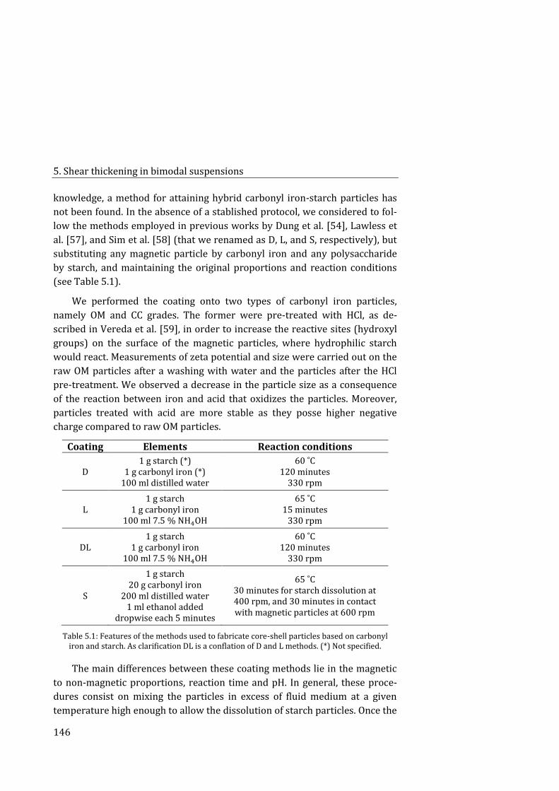
5. Shear thickening in bimodal suspensions
146
knowledge, a method for attaining hybrid carbonyl iron-starch particles has
not been found. In the absence of a stablished protocol, we considered to fol-
low the methods employed in previous works by Dung et al. [54], Lawless et
al. [57], and Sim et al. [58] (that we renamed as D, L, and S, respectively), but
substituting any magnetic particle by carbonyl iron and any polysaccharide
by starch, and maintaining the original proportions and reaction conditions
(see Table 5.1).
We performed the coating onto two types of carbonyl iron particles,
namely OM and CC grades. The former were pre-treated with HCl, as de-
scribed in Vereda et al. [59], in order to increase the reactive sites (hydroxyl
groups) on the surface of the magnetic particles, where hydrophilic starch
would react. Measurements of zeta potential and size were carried out on the
raw OM particles after a washing with water and the particles after the HCl
pre-treatment. We observed a decrease in the particle size as a consequence
of the reaction between iron and acid that oxidizes the particles. Moreover,
particles treated with acid are more stable as they posse higher negative
charge compared to raw OM particles.
Coating Elements Reaction conditions
D 1 g starch (*)
1 g carbonyl iron (*) 100 ml distilled water
60 ˚C 120 minutes
330 rpm
L 1 g starch
1 g carbonyl iron 100 ml 7.5 % NH4OH
65 ˚C 15 minutes
330 rpm
DL 1 g starch
1 g carbonyl iron 100 ml 7.5 % NH4OH
60 ˚C 120 minutes
330 rpm
S
1 g starch 20 g carbonyl iron
200 ml distilled water 1 ml ethanol added
dropwise each 5 minutes
65 ˚C 30 minutes for starch dissolution at 400 rpm, and 30 minutes in contact with magnetic particles at 600 rpm
Table 5.1: Features of the methods used to fabricate core-shell particles based on carbonyl iron and starch. As clarification DL is a conflation of D and L methods. (*) Not specified.
The main differences between these coating methods lie in the magnetic
to non-magnetic proportions, reaction time and pH. In general, these proce-
dures consist on mixing the particles in excess of fluid medium at a given
temperature high enough to allow the dissolution of starch particles. Once the
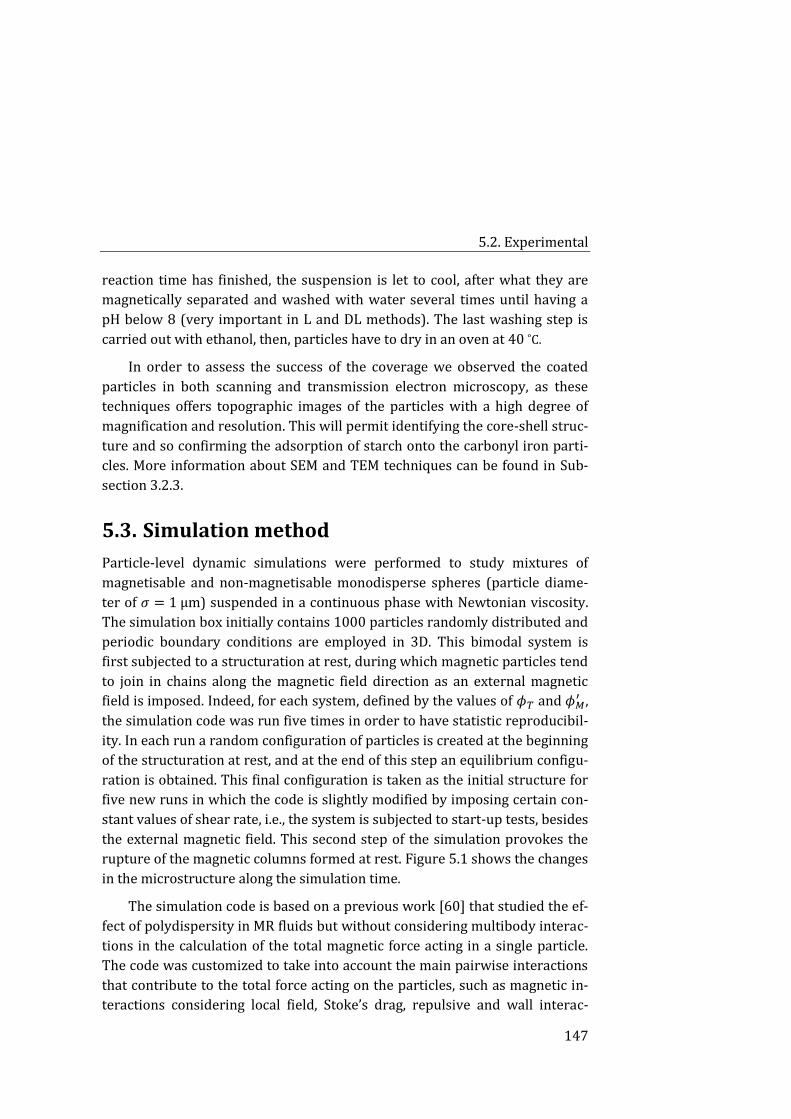
5.2. Experimental
147
reaction time has finished, the suspension is let to cool, after what they are
magnetically separated and washed with water several times until having a
pH below 8 (very important in L and DL methods). The last washing step is
carried out with ethanol, then, particles have to dry in an oven at 40 ˚C.
In order to assess the success of the coverage we observed the coated
particles in both scanning and transmission electron microscopy, as these
techniques offers topographic images of the particles with a high degree of
magnification and resolution. This will permit identifying the core-shell struc-
ture and so confirming the adsorption of starch onto the carbonyl iron parti-
cles. More information about SEM and TEM techniques can be found in Sub-
section 3.2.3.
Simulation method 5.3.
Particle-level dynamic simulations were performed to study mixtures of
magnetisable and non-magnetisable monodisperse spheres (particle diame-
ter of 𝜎 = 1 μm) suspended in a continuous phase with Newtonian viscosity.
The simulation box initially contains 1000 particles randomly distributed and
periodic boundary conditions are employed in 3D. This bimodal system is
first subjected to a structuration at rest, during which magnetic particles tend
to join in chains along the magnetic field direction as an external magnetic
field is imposed. Indeed, for each system, defined by the values of 𝜙𝑇 and 𝜙𝑀′ ,
the simulation code was run five times in order to have statistic reproducibil-
ity. In each run a random configuration of particles is created at the beginning
of the structuration at rest, and at the end of this step an equilibrium configu-
ration is obtained. This final configuration is taken as the initial structure for
five new runs in which the code is slightly modified by imposing certain con-
stant values of shear rate, i.e., the system is subjected to start-up tests, besides
the external magnetic field. This second step of the simulation provokes the
rupture of the magnetic columns formed at rest. Figure 5.1 shows the changes
in the microstructure along the simulation time.
The simulation code is based on a previous work [60] that studied the ef-
fect of polydispersity in MR fluids but without considering multibody interac-
tions in the calculation of the total magnetic force acting in a single particle.
The code was customized to take into account the main pairwise interactions
that contribute to the total force acting on the particles, such as magnetic in-
teractions considering local field, Stoke’s drag, repulsive and wall interac-
5. Shear thickening in bimodal suspensions
148
tions, as well as stochastic forces related to the motion of Brownian particles.
The Langevin equation of motion Equation 5.1 is solved at each simulation
time and particles move to their new positions. These interactions are de-
scribed in detail in Subsection 3.3.1.
𝑚𝑖
𝑑2𝒓𝒊
𝑑𝑡2= ∑ 𝑭𝒊
𝒆 + 𝑭𝒊𝒉 + 𝑭𝒊
𝒃 , (5.1)
It is worth saying that in a first approximation lubrication forces were not
introduced into the simulation code because of their complexity. Then, they
were fully defined, as it is shown in Subsection 3.3.1, as we considered they
should have a relevant role in the behaviour of concentrated systems. How-
ever, the maximum total concentration achievable in these monodisperse sys-
tems was low to observe shear thickening, so that the fact of avoiding hydro-
dynamic lubrication did not imply great change in the evolution of the system.
Figure 5.1: Simulation box for a system of 1000 monodisperse particles with 𝜙𝑇 = 0.20 and 𝜙𝑀
′ = 0.30 at different simulation times. White and grey spheres represent non-magnetic and magnetic particles, respectively. a) Start of the simulation process, where
particles are randomly located, b) Evolution of particle structuration at rest in the form of magnetic columnar aggregates under the presence of the magnetic field, and c) Shear
stage under application of magnetic field.
In order to compare the effect of considering or not lubrication forces we
ran two programs at the same time, one with the full simulation code and
other taking into account only Stokes’ drag. Due to the high computational
cost derived from the complexity of lubrication interactions, we chose a rela-
tively low total volume fraction. The normalized total magnetic energy during
structuration is shown in Figure 5.2.
As can be observed, the incorporation of lubrication forces supposes a
decrease in the absolute value of the magnetic energy at each simulation time,
which indicates that magnetic structures are less stable. The delay in black
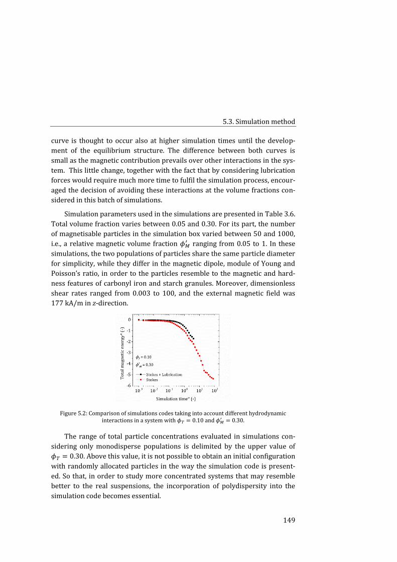
5.3. Simulation method
149
curve is thought to occur also at higher simulation times until the develop-
ment of the equilibrium structure. The difference between both curves is
small as the magnetic contribution prevails over other interactions in the sys-
tem. This little change, together with the fact that by considering lubrication
forces would require much more time to fulfil the simulation process, encour-
aged the decision of avoiding these interactions at the volume fractions con-
sidered in this batch of simulations.
Simulation parameters used in the simulations are presented in Table 3.6.
Total volume fraction varies between 0.05 and 0.30. For its part, the number
of magnetisable particles in the simulation box varied between 50 and 1000,
i.e., a relative magnetic volume fraction 𝜙𝑀′ ranging from 0.05 to 1. In these
simulations, the two populations of particles share the same particle diameter
for simplicity, while they differ in the magnetic dipole, module of Young and
Poisson’s ratio, in order to the particles resemble to the magnetic and hard-
ness features of carbonyl iron and starch granules. Moreover, dimensionless
shear rates ranged from 0.003 to 100, and the external magnetic field was
177 kA/m in z-direction.
Figure 5.2: Comparison of simulations codes taking into account different hydrodynamic interactions in a system with 𝜙𝑇 = 0.10 and 𝜙𝑀
′ = 0.30.
The range of total particle concentrations evaluated in simulations con-
sidering only monodisperse populations is delimited by the upper value of
𝜙𝑇 = 0.30. Above this value, it is not possible to obtain an initial configuration
with randomly allocated particles in the way the simulation code is present-
ed. So that, in order to study more concentrated systems that may resemble
better to the real suspensions, the incorporation of polydispersity into the
simulation code becomes essential.
5. Shear thickening in bimodal suspensions
150
In this sense, a second scenario of particle-level dynamic simulations is
carried out by considering polydispersity in both magnetic and non-magnetic
populations, while the rest of the simulation code is maintained. Polydispersi-
ty index (PDI) is a parameter related to the standard deviation 𝜈 through the
expression 𝑃𝐷𝐼 = 3𝜈2 + 1. According to the size distribution analysis of corn-
starch used in experiments, 𝑃𝐷𝐼𝑆𝑡𝑎𝑟𝑐ℎ,25°𝐶 = 1.388 (see Table 3.3), so that
= 0.36 . For the sake of simplicity, standard deviation of both particle popula-
tions will take this value. Moreover, it is imposed in the simulation code that
the ratio between non-magnetic and magnetic mean particle diameters is 10,
similarly to the experimental case, namely 𝜎𝑁 = 10 μm, and 𝜎𝑀 = 1 μm.
The use of this value of standard PDI allows for having more concentrat-
ed initial configurations. Comparably to the first scenario, at this point we
study the rheological behaviour of hybrid systems composed of magnetisable
and non-magnetisable spherical and polydisperse particles, both at rest and
under shear flow, subjected to a constant magnetic field.
Results and discussion 5.4.
Rheological results of bimodal suspensions are presented in this section.
First, we explore the effect of the addition of magnetic particles to a model ST
fluid in Subsection 5.4.1. Then, in Subsection 5.4.2the rheological behaviour of
MRST fluids was investigated using core-shell particles of carbonyl iron coat-
ed with starch in the formulation of concentrated hybrid suspensions. After
that, we compare rheological results of unimodal and these two types of hy-
brid suspensions in Subsection 5.4.3. Final subsections are devoted to the
particle-level simulation results of bimodal systems, i.e., composed by mag-
netisable and non-magnetisable populations. The effects of magnetic field,
particle concentration and volume fraction ratios are evaluated for monodis-
perse and polydisperse systems, in Subsection 5.4.4 and Subsection 5.4.5, re-
spectively.
Bimodal MRST suspensions 5.4.1.
In this subsection we study the rheological properties of bimodal suspensions
in water. The disperse phase is constituted by two types of particles: starch
and carbonyl iron (CC grade). The effect of the iron concentration and mag-
netic field on the rheological response of these MRST fluids is investigated.
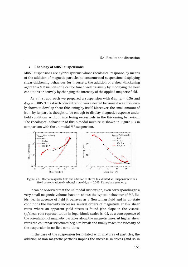
5.4. Results and discussion
151
Rheology of MRST suspensions
MRST suspensions are hybrid systems whose rheological response, by means
of the addition of magnetic particles to concentrated suspensions displaying
shear-thickening behaviour (or inversely, the addition of a shear-thickening
agent to a MR suspension), can be tuned well passively by modifying the flow
conditions or actively by changing the intensity of the applied magnetic field.
As a first approach we prepared a suspension with 𝜙𝑆𝑡𝑎𝑟𝑐ℎ = 0.36 and
𝜙𝐶𝐶 = 0.005. This starch concentration was selected because it was previous-
ly shown to develop shear thickening by itself. Moreover, the small amount of
iron, by its part, is thought to be enough to display magnetic response under
field conditions without interfering excessively in the thickening behaviour.
The rheological behaviour of this bimodal mixture is shown in Figure 5.3 in
comparison with the unimodal MR suspension.
Figure 5.3: Effect of magnetic field and addition of starch to a diluted MR suspension with a fixed concentration of carbonyl iron of 𝜙𝐶𝐶 = 0.005. Plate-plate geometry.
It can be observed that the unimodal suspension, even corresponding to a
very small magnetic volume fraction, shows the typical behaviour of MR flu-
ids, i.e., in absence of field it behaves as a Newtonian fluid and in on-state
conditions the viscosity increases several orders of magnitude at low shear
rates, where an apparent yield stress is found (the slope in the viscosi-
ty/shear rate representation in logarithmic scales is -1), as a consequence of
the orientation of magnetic particles along the magnetic lines. At higher shear
rates the columnar structures begin to break and finally reach the viscosity of
the suspension in no-field conditions.
In the case of the suspension formulated with mixtures of particles, the
addition of non-magnetic particles implies the increase in stress (and so in
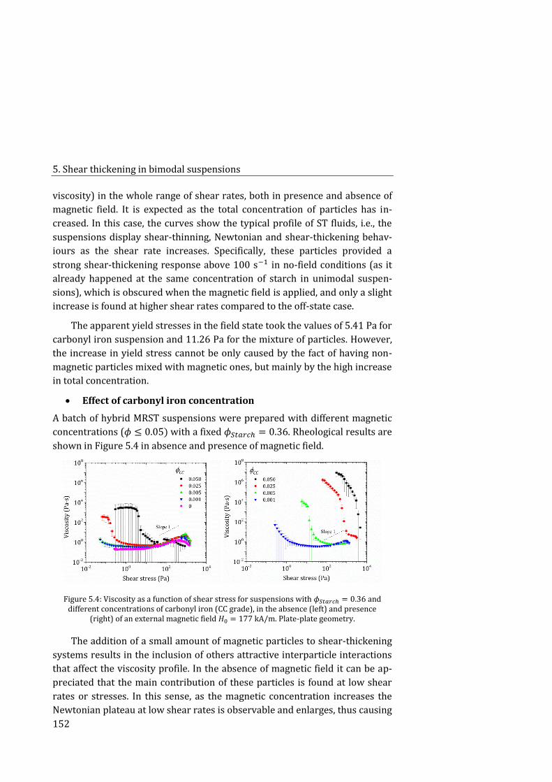
5. Shear thickening in bimodal suspensions
152
viscosity) in the whole range of shear rates, both in presence and absence of
magnetic field. It is expected as the total concentration of particles has in-
creased. In this case, the curves show the typical profile of ST fluids, i.e., the
suspensions display shear-thinning, Newtonian and shear-thickening behav-
iours as the shear rate increases. Specifically, these particles provided a
strong shear-thickening response above 100 s−1 in no-field conditions (as it
already happened at the same concentration of starch in unimodal suspen-
sions), which is obscured when the magnetic field is applied, and only a slight
increase is found at higher shear rates compared to the off-state case.
The apparent yield stresses in the field state took the values of 5.41 Pa for
carbonyl iron suspension and 11.26 Pa for the mixture of particles. However,
the increase in yield stress cannot be only caused by the fact of having non-
magnetic particles mixed with magnetic ones, but mainly by the high increase
in total concentration.
Effect of carbonyl iron concentration
A batch of hybrid MRST suspensions were prepared with different magnetic
concentrations (𝜙 ≤ 0.05) with a fixed 𝜙𝑆𝑡𝑎𝑟𝑐ℎ = 0.36. Rheological results are
shown in Figure 5.4 in absence and presence of magnetic field.
Figure 5.4: Viscosity as a function of shear stress for suspensions with 𝜙𝑆𝑡𝑎𝑟𝑐ℎ = 0.36 and different concentrations of carbonyl iron (CC grade), in the absence (left) and presence
(right) of an external magnetic field 𝐻0 = 177 kA/m. Plate-plate geometry.
The addition of a small amount of magnetic particles to shear-thickening
systems results in the inclusion of others attractive interparticle interactions
that affect the viscosity profile. In the absence of magnetic field it can be ap-
preciated that the main contribution of these particles is found at low shear
rates or stresses. In this sense, as the magnetic concentration increases the
Newtonian plateau at low shear rates is observable and enlarges, thus causing
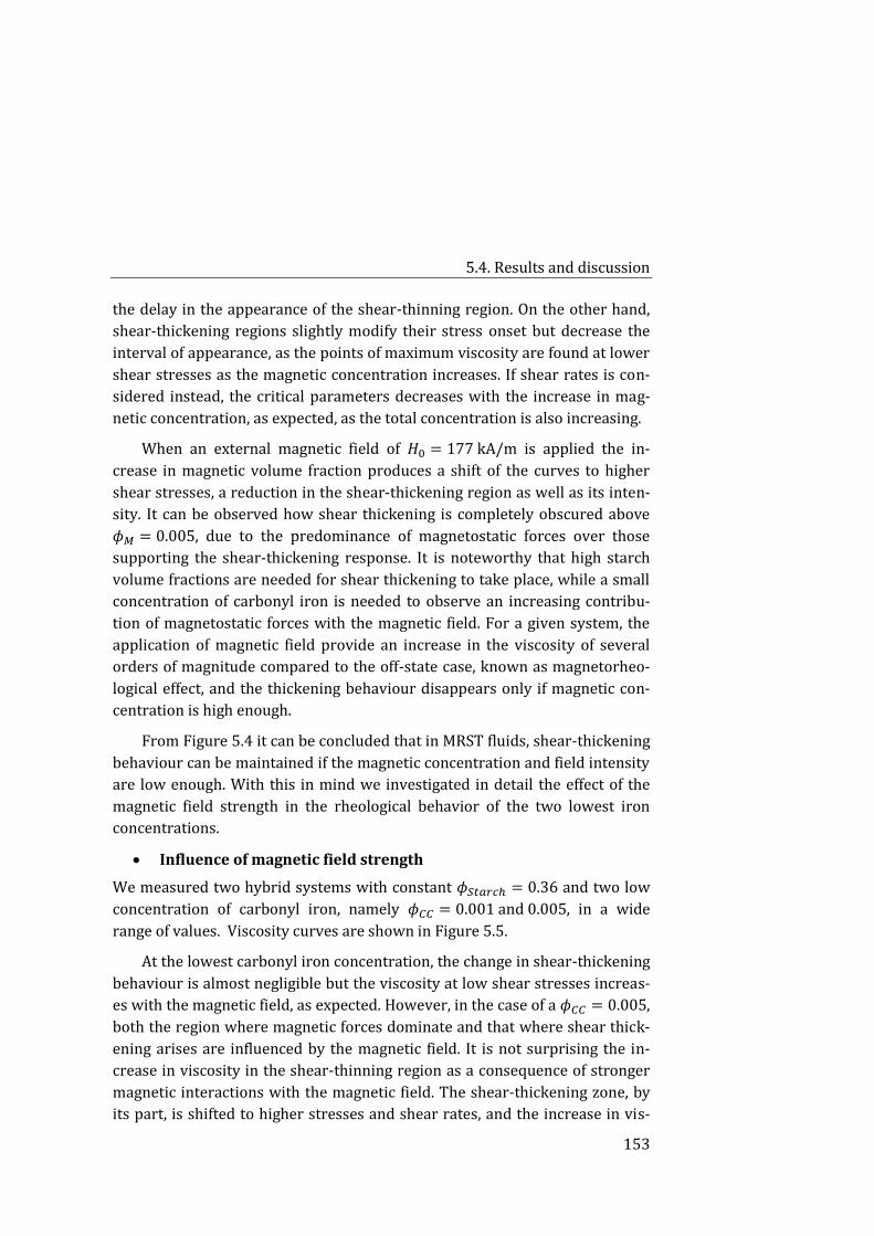
5.4. Results and discussion
153
the delay in the appearance of the shear-thinning region. On the other hand,
shear-thickening regions slightly modify their stress onset but decrease the
interval of appearance, as the points of maximum viscosity are found at lower
shear stresses as the magnetic concentration increases. If shear rates is con-
sidered instead, the critical parameters decreases with the increase in mag-
netic concentration, as expected, as the total concentration is also increasing.
When an external magnetic field of 𝐻0 = 177 kA/m is applied the in-
crease in magnetic volume fraction produces a shift of the curves to higher
shear stresses, a reduction in the shear-thickening region as well as its inten-
sity. It can be observed how shear thickening is completely obscured above
𝜙𝑀 = 0.005, due to the predominance of magnetostatic forces over those
supporting the shear-thickening response. It is noteworthy that high starch
volume fractions are needed for shear thickening to take place, while a small
concentration of carbonyl iron is needed to observe an increasing contribu-
tion of magnetostatic forces with the magnetic field. For a given system, the
application of magnetic field provide an increase in the viscosity of several
orders of magnitude compared to the off-state case, known as magnetorheo-
logical effect, and the thickening behaviour disappears only if magnetic con-
centration is high enough.
From Figure 5.4 it can be concluded that in MRST fluids, shear-thickening
behaviour can be maintained if the magnetic concentration and field intensity
are low enough. With this in mind we investigated in detail the effect of the
magnetic field strength in the rheological behavior of the two lowest iron
concentrations.
Influence of magnetic field strength
We measured two hybrid systems with constant 𝜙𝑆𝑡𝑎𝑟𝑐ℎ = 0.36 and two low
concentration of carbonyl iron, namely 𝜙𝐶𝐶 = 0.001 and 0.005, in a wide
range of values. Viscosity curves are shown in Figure 5.5.
At the lowest carbonyl iron concentration, the change in shear-thickening
behaviour is almost negligible but the viscosity at low shear stresses increas-
es with the magnetic field, as expected. However, in the case of a 𝜙𝐶𝐶 = 0.005,
both the region where magnetic forces dominate and that where shear thick-
ening arises are influenced by the magnetic field. It is not surprising the in-
crease in viscosity in the shear-thinning region as a consequence of stronger
magnetic interactions with the magnetic field. The shear-thickening zone, by
its part, is shifted to higher stresses and shear rates, and the increase in vis-
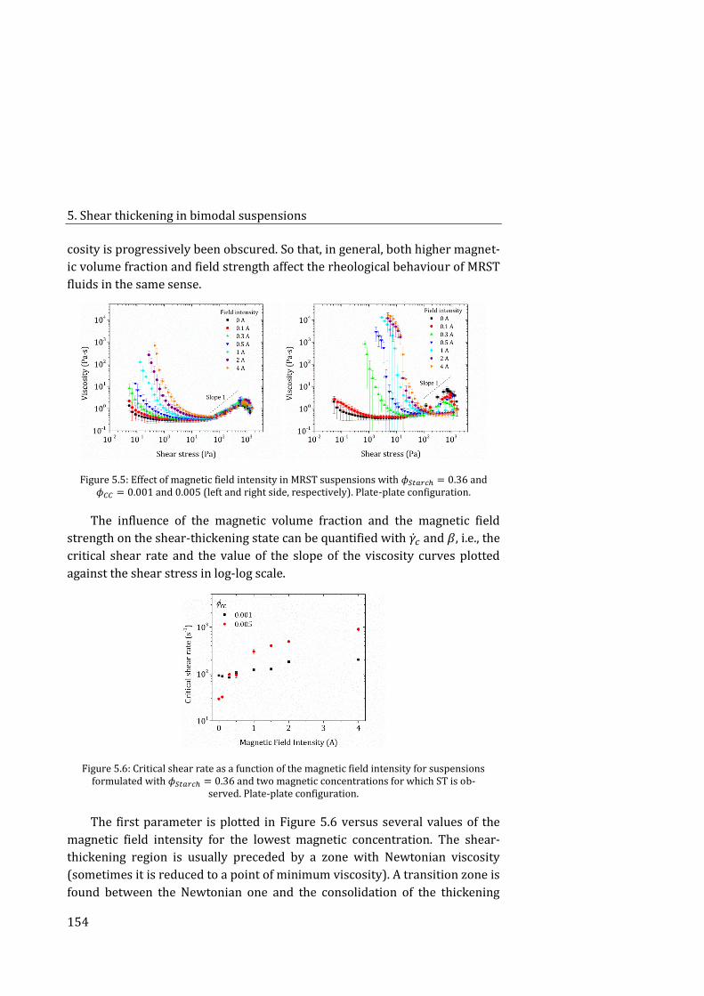
5. Shear thickening in bimodal suspensions
154
cosity is progressively been obscured. So that, in general, both higher magnet-
ic volume fraction and field strength affect the rheological behaviour of MRST
fluids in the same sense.
Figure 5.5: Effect of magnetic field intensity in MRST suspensions with 𝜙𝑆𝑡𝑎𝑟𝑐ℎ = 0.36 and 𝜙𝐶𝐶 = 0.001 and 0.005 (left and right side, respectively). Plate-plate configuration.
The influence of the magnetic volume fraction and the magnetic field
strength on the shear-thickening state can be quantified with �̇�𝑐 and 𝛽, i.e., the
critical shear rate and the value of the slope of the viscosity curves plotted
against the shear stress in log-log scale.
Figure 5.6: Critical shear rate as a function of the magnetic field intensity for suspensions formulated with 𝜙𝑆𝑡𝑎𝑟𝑐ℎ = 0.36 and two magnetic concentrations for which ST is ob-
served. Plate-plate configuration.
The first parameter is plotted in Figure 5.6 versus several values of the
magnetic field intensity for the lowest magnetic concentration. The shear-
thickening region is usually preceded by a zone with Newtonian viscosity
(sometimes it is reduced to a point of minimum viscosity). A transition zone is
found between the Newtonian one and the consolidation of the thickening
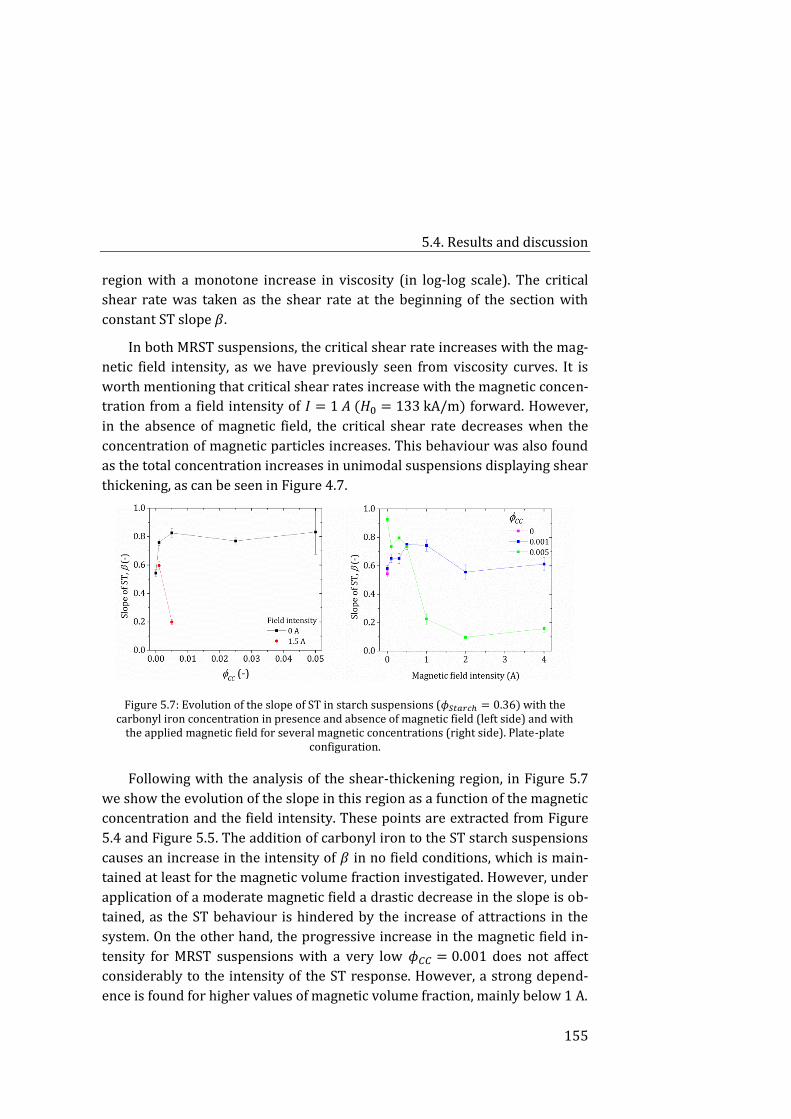
5.4. Results and discussion
155
region with a monotone increase in viscosity (in log-log scale). The critical
shear rate was taken as the shear rate at the beginning of the section with
constant ST slope 𝛽.
In both MRST suspensions, the critical shear rate increases with the mag-
netic field intensity, as we have previously seen from viscosity curves. It is
worth mentioning that critical shear rates increase with the magnetic concen-
tration from a field intensity of 𝐼 = 1 𝐴 (𝐻0 = 133 kA/m) forward. However,
in the absence of magnetic field, the critical shear rate decreases when the
concentration of magnetic particles increases. This behaviour was also found
as the total concentration increases in unimodal suspensions displaying shear
thickening, as can be seen in Figure 4.7.
Figure 5.7: Evolution of the slope of ST in starch suspensions (𝜙𝑆𝑡𝑎𝑟𝑐ℎ = 0.36) with the carbonyl iron concentration in presence and absence of magnetic field (left side) and with
the applied magnetic field for several magnetic concentrations (right side). Plate-plate configuration.
Following with the analysis of the shear-thickening region, in Figure 5.7
we show the evolution of the slope in this region as a function of the magnetic
concentration and the field intensity. These points are extracted from Figure
5.4 and Figure 5.5. The addition of carbonyl iron to the ST starch suspensions
causes an increase in the intensity of 𝛽 in no field conditions, which is main-
tained at least for the magnetic volume fraction investigated. However, under
application of a moderate magnetic field a drastic decrease in the slope is ob-
tained, as the ST behaviour is hindered by the increase of attractions in the
system. On the other hand, the progressive increase in the magnetic field in-
tensity for MRST suspensions with a very low 𝜙𝐶𝐶 = 0.001 does not affect
considerably to the intensity of the ST response. However, a strong depend-
ence is found for higher values of magnetic volume fraction, mainly below 1 A.
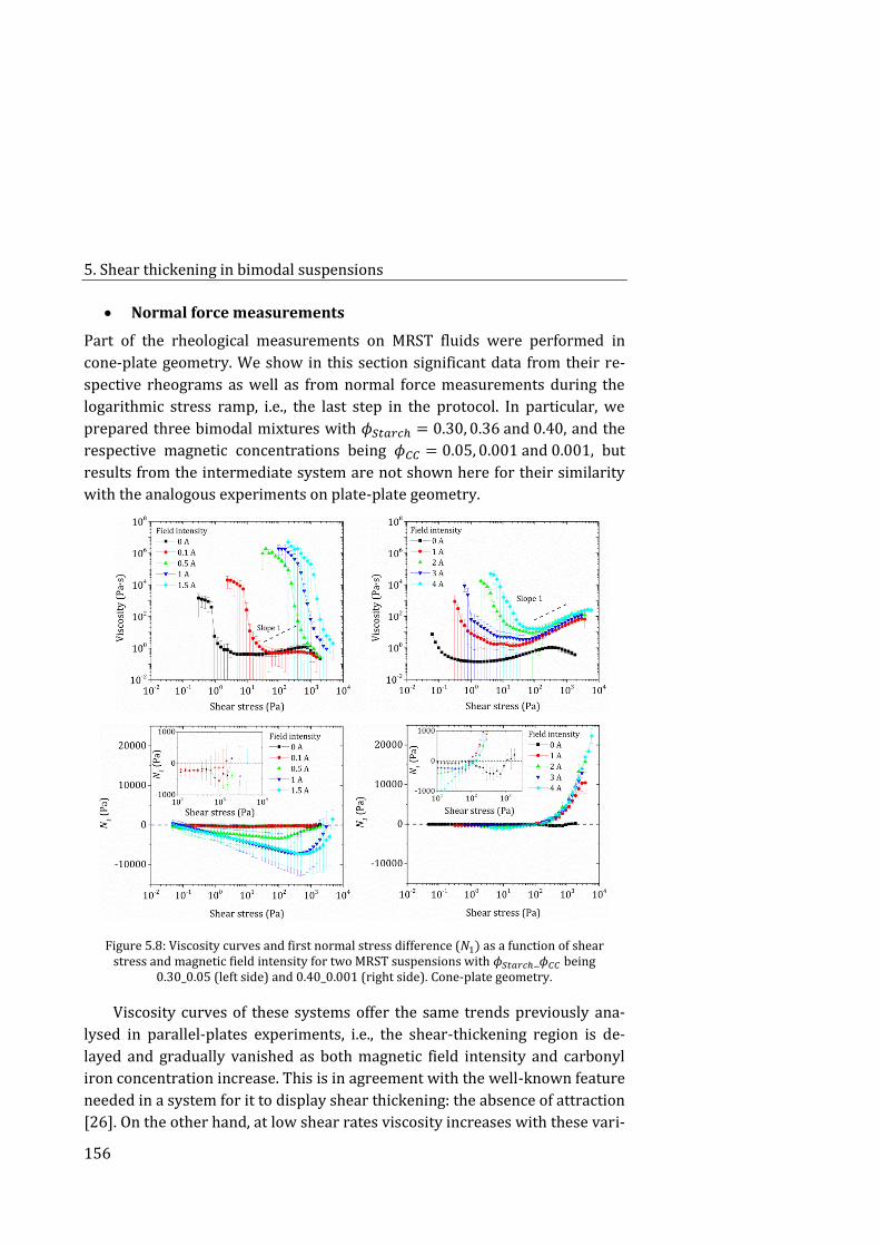
5. Shear thickening in bimodal suspensions
156
Normal force measurements
Part of the rheological measurements on MRST fluids were performed in
cone-plate geometry. We show in this section significant data from their re-
spective rheograms as well as from normal force measurements during the
logarithmic stress ramp, i.e., the last step in the protocol. In particular, we
prepared three bimodal mixtures with 𝜙𝑆𝑡𝑎𝑟𝑐ℎ = 0.30, 0.36 and 0.40, and the
respective magnetic concentrations being 𝜙𝐶𝐶 = 0.05, 0.001 and 0.001, but
results from the intermediate system are not shown here for their similarity
with the analogous experiments on plate-plate geometry.
Figure 5.8: Viscosity curves and first normal stress difference (𝑁1) as a function of shear stress and magnetic field intensity for two MRST suspensions with 𝜙𝑆𝑡𝑎𝑟𝑐ℎ_𝜙𝐶𝐶 being
0.30_0.05 (left side) and 0.40_0.001 (right side). Cone-plate geometry.
Viscosity curves of these systems offer the same trends previously ana-
lysed in parallel-plates experiments, i.e., the shear-thickening region is de-
layed and gradually vanished as both magnetic field intensity and carbonyl
iron concentration increase. This is in agreement with the well-known feature
needed in a system for it to display shear thickening: the absence of attraction
[26]. On the other hand, at low shear rates viscosity increases with these vari-
5.4. Results and discussion
157
ables due to the formation of magnetic columnar aggregates as a consequence
of the induced magnetic dipolar interactions among carbonyl iron particles,
which may lead to yield stress, and break as shear rate progresses.
The effect of the applied magnetic field on the normal force depends a lot
on the concentration of magnetic particles in these hybrid suspensions. In the
left side, where 𝜙𝐶𝐶 = 0.05, the normal force (and so 𝑁1) continuously de-
creases with the applied field up to a minimum at a given shear stress. After
this minimum, the response is reversed. This characteristic stress seems to
coincide to the onset of the steep diminishing in viscosity in the graph above,
corresponding to the yield stress. A similar behaviour was previously ob-
served [61]. They prepared MR suspensions at a higher concentration (10 %)
for which the solid phase was only composed by micronsized magnetic parti-
cles. These unimodal suspensions showed a normal force dependence with
particle concentration and magnetic field, as expected. Moreover, the normal
force, developed as a consequence of the application of the magnetic field,
was always positive in the whole interval of shear rates. They found two plat-
eaus at low and high shear rates, while at intermediate values the normal
force reached a minimum, which was independent of the magnetic field and
was related to the pre-yield regime.
In our system with starch (0.30_0.05) we also have this minimum in
normal force and observe that after this minimum the suspension also start to
flow, but the related shear stress varies with the field, as yield stress does.
The main difference with this work in literature comes from the sign in nor-
mal force, which in the case of our bimodal suspensions is negative. This fact
may be due to the great contribution of the non-magnetic particles. Although
a crossover stress is not observed in the five curves (the tests have to be
aborted when the sample is ejected out of the geometry), it seems to be prox-
imately the same for a given ratio of magnetic and non-magnetic particles,
regarding the tendency of the curves, as it occurs with the system with a dif-
ferent ratio of starch to carbonyl iron (case of 0.36_0.001).
On the other hand, in the case of highly concentrated MR suspensions, de
Vicente et al. [62] found positive values of the normal force upon the applica-
tion of high enough magnetic fields as a consequence of the gap spanning oc-
curring by the formation of magnetic chains. During shearing these structures
bend and, because of such a high concentration, chains join in stronger struc-
tures that also provoke the system expansion. However the curve profile of
normal force against shear stress reaches a maximum (instead of a minimum)
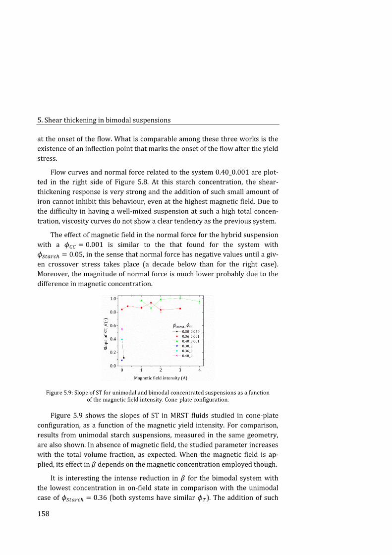
5. Shear thickening in bimodal suspensions
158
at the onset of the flow. What is comparable among these three works is the
existence of an inflection point that marks the onset of the flow after the yield
stress.
Flow curves and normal force related to the system 0.40_0.001 are plot-
ted in the right side of Figure 5.8. At this starch concentration, the shear-
thickening response is very strong and the addition of such small amount of
iron cannot inhibit this behaviour, even at the highest magnetic field. Due to
the difficulty in having a well-mixed suspension at such a high total concen-
tration, viscosity curves do not show a clear tendency as the previous system.
The effect of magnetic field in the normal force for the hybrid suspension
with a 𝜙𝐶𝐶 = 0.001 is similar to the that found for the system with
𝜙𝑆𝑡𝑎𝑟𝑐ℎ = 0.05, in the sense that normal force has negative values until a giv-
en crossover stress takes place (a decade below than for the right case).
Moreover, the magnitude of normal force is much lower probably due to the
difference in magnetic concentration.
Figure 5.9: Slope of ST for unimodal and bimodal concentrated suspensions as a function of the magnetic field intensity. Cone-plate configuration.
Figure 5.9 shows the slopes of ST in MRST fluids studied in cone-plate
configuration, as a function of the magnetic yield intensity. For comparison,
results from unimodal starch suspensions, measured in the same geometry,
are also shown. In absence of magnetic field, the studied parameter increases
with the total volume fraction, as expected. When the magnetic field is ap-
plied, its effect in 𝛽 depends on the magnetic concentration employed though.
It is interesting the intense reduction in 𝛽 for the bimodal system with
the lowest concentration in on-field state in comparison with the unimodal
case of 𝜙𝑆𝑡𝑎𝑟𝑐ℎ = 0.36 (both systems have similar 𝜙𝑇). The addition of such
5.4. Results and discussion
159
amount of carbonyl iron greatly increases the attraction in the suspension,
and so the ST behaviour is weakened in on-state field conditions. However, it
is striking the noticeable increment in the ST response for MRST suspensions
with a 𝜙𝐶𝐶 = 0.001, with a value of 𝛽 that is nearly independent of the mag-
netic field and very close to unity, mainly in the most concentrated case. It is
reasonable to think that these rheological measurements are slightly overes-
timated, as cone-plate geometry is not the most adequate configuration when
the magnetic field is applied. However, both Figure 5.7 and Figure 5.9 agree
on the great dependence of the slope of the ST on the magnetic concentration
when the magnetic field is applied. This suggests that there is a critical vol-
ume fraction of carbonyl iron that somehow reinforces the microstructure of
the system in the range of shear stresses where the shear thickening occurs.
So that, besides the possibility of tuning the rheological behaviour of this sys-
tem by means of the application of an external magnetic field (which mainly
affects the low shear rate region and the onset of the thickening), a transition
from continuous to near discontinuous shear thickening is simply achieved by
the addition of a small amount of non-magnetic particles to the system.
Suspensions of hybrid core-shell particles 5.4.2.
Environmental scanning electron microscopy (ESEM)
We performed analysis in secondary electrons (SE) and circular backscatter-
ing (CBS) modes; the first shows the topography of the surface and the other
highlights differences in concentration. The resolution in ESEM depends on
the intensity of the incident primary electron beam. All images in the SE mode
were taken at 5 kV. However, in the CBS mode the beam is set at 5 kV but the
slide is set at 2 kV. With this trick, the beam reaches the sample decelerated,
and the landing velocity of the electrons in the surface of the sample is actual-
ly 3 kV. This reduction is necessary because we expect a narrow thickness of
starch coating the carbonyl iron particles (of several nanometres). A higher
intensity of the incident beam involves more penetration, and micrographs
would show only iron. In this sense, the micrographs obtained in SE mode
have a better resolution than in the other mode, but with this last, changes in
composition can be better observed with different brightness (compare im-
ages in Figure 5.10 with lower magnification).
In Figure 5.10 we show some micrographs of bimodal core-shell particles
obtained following the methods of Table 5.1. Each image will be named ac-
cording the type of particle and coating method employed, e.g., OM/D (a) and
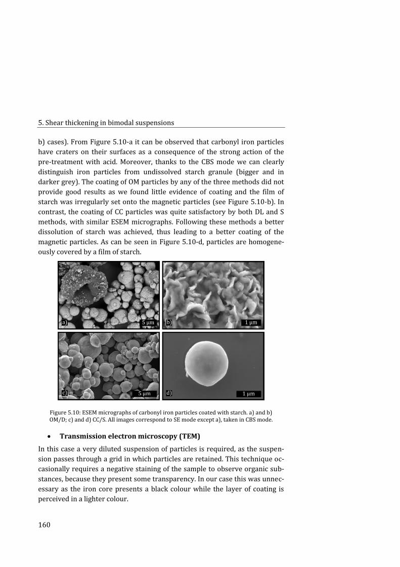
5. Shear thickening in bimodal suspensions
160
b) cases). From Figure 5.10-a it can be observed that carbonyl iron particles
have craters on their surfaces as a consequence of the strong action of the
pre-treatment with acid. Moreover, thanks to the CBS mode we can clearly
distinguish iron particles from undissolved starch granule (bigger and in
darker grey). The coating of OM particles by any of the three methods did not
provide good results as we found little evidence of coating and the film of
starch was irregularly set onto the magnetic particles (see Figure 5.10-b). In
contrast, the coating of CC particles was quite satisfactory by both DL and S
methods, with similar ESEM micrographs. Following these methods a better
dissolution of starch was achieved, thus leading to a better coating of the
magnetic particles. As can be seen in Figure 5.10-d, particles are homogene-
ously covered by a film of starch.
Figure 5.10: ESEM micrographs of carbonyl iron particles coated with starch. a) and b) OM/D; c) and d) CC/S. All images correspond to SE mode except a), taken in CBS mode.
Transmission electron microscopy (TEM)
In this case a very diluted suspension of particles is required, as the suspen-
sion passes through a grid in which particles are retained. This technique oc-
casionally requires a negative staining of the sample to observe organic sub-
stances, because they present some transparency. In our case this was unnec-
essary as the iron core presents a black colour while the layer of coating is
perceived in a lighter colour.
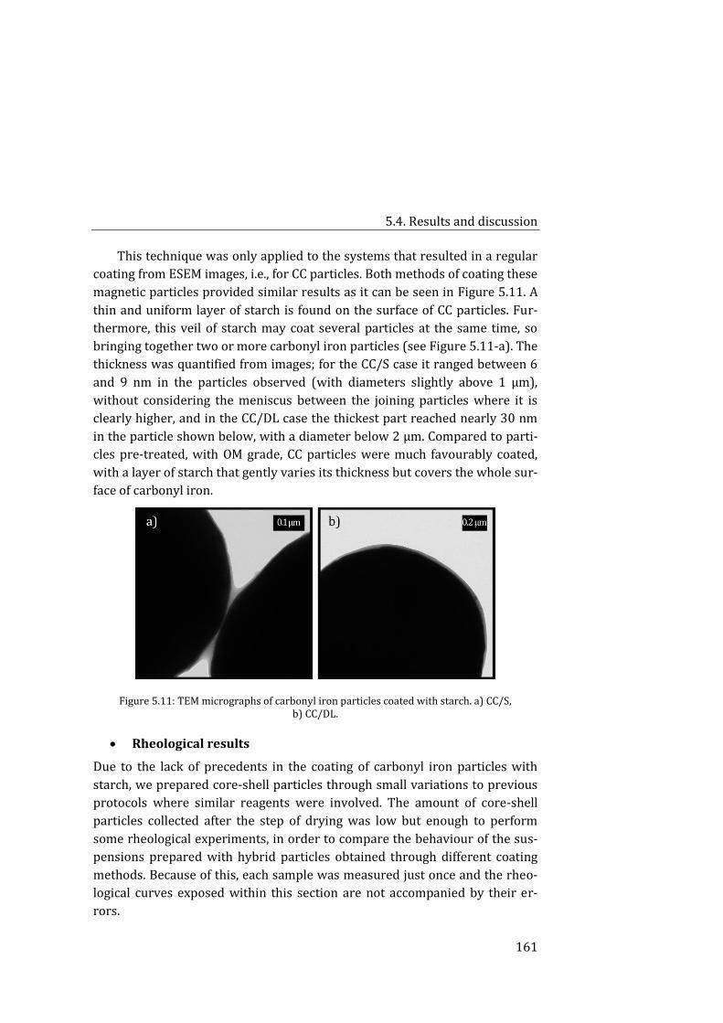
5.4. Results and discussion
161
This technique was only applied to the systems that resulted in a regular
coating from ESEM images, i.e., for CC particles. Both methods of coating these
magnetic particles provided similar results as it can be seen in Figure 5.11. A
thin and uniform layer of starch is found on the surface of CC particles. Fur-
thermore, this veil of starch may coat several particles at the same time, so
bringing together two or more carbonyl iron particles (see Figure 5.11-a). The
thickness was quantified from images; for the CC/S case it ranged between 6
and 9 nm in the particles observed (with diameters slightly above 1 µm),
without considering the meniscus between the joining particles where it is
clearly higher, and in the CC/DL case the thickest part reached nearly 30 nm
in the particle shown below, with a diameter below 2 µm. Compared to parti-
cles pre-treated, with OM grade, CC particles were much favourably coated,
with a layer of starch that gently varies its thickness but covers the whole sur-
face of carbonyl iron.
Figure 5.11: TEM micrographs of carbonyl iron particles coated with starch. a) CC/S, b) CC/DL.
Rheological results
Due to the lack of precedents in the coating of carbonyl iron particles with
starch, we prepared core-shell particles through small variations to previous
protocols where similar reagents were involved. The amount of core-shell
particles collected after the step of drying was low but enough to perform
some rheological experiments, in order to compare the behaviour of the sus-
pensions prepared with hybrid particles obtained through different coating
methods. Because of this, each sample was measured just once and the rheo-
logical curves exposed within this section are not accompanied by their er-
rors.
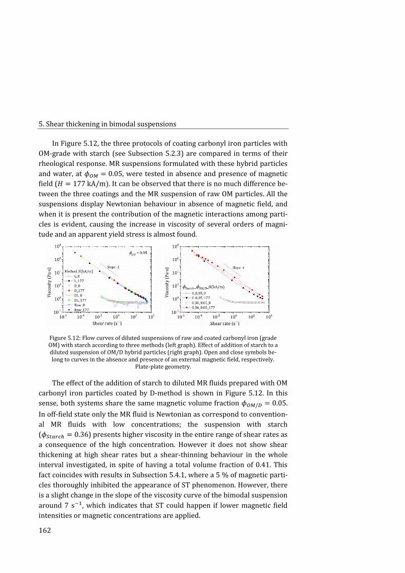
5. Shear thickening in bimodal suspensions
162
In Figure 5.12, the three protocols of coating carbonyl iron particles with
OM-grade with starch (see Subsection 5.2.3) are compared in terms of their
rheological response. MR suspensions formulated with these hybrid particles
and water, at 𝜙𝑂𝑀 = 0.05, were tested in absence and presence of magnetic
field (𝐻 = 177 kA/m). It can be observed that there is no much difference be-
tween the three coatings and the MR suspension of raw OM particles. All the
suspensions display Newtonian behaviour in absence of magnetic field, and
when it is present the contribution of the magnetic interactions among parti-
cles is evident, causing the increase in viscosity of several orders of magni-
tude and an apparent yield stress is almost found.
Figure 5.12: Flow curves of diluted suspensions of raw and coated carbonyl iron (grade OM) with starch according to three methods (left graph). Effect of addition of starch to a diluted suspension of OM/D hybrid particles (right graph). Open and close symbols be-long to curves in the absence and presence of an external magnetic field, respectively.
Plate-plate geometry.
The effect of the addition of starch to diluted MR fluids prepared with OM
carbonyl iron particles coated by D-method is shown in Figure 5.12. In this
sense, both systems share the same magnetic volume fraction 𝜙𝑂𝑀/𝐷 = 0.05.
In off-field state only the MR fluid is Newtonian as correspond to convention-
al MR fluids with low concentrations; the suspension with starch
(𝜙𝑆𝑡𝑎𝑟𝑐ℎ = 0.36) presents higher viscosity in the entire range of shear rates as
a consequence of the high concentration. However it does not show shear
thickening at high shear rates but a shear-thinning behaviour in the whole
interval investigated, in spite of having a total volume fraction of 0.41. This
fact coincides with results in Subsection 5.4.1, where a 5 % of magnetic parti-
cles thoroughly inhibited the appearance of ST phenomenon. However, there
is a slight change in the slope of the viscosity curve of the bimodal suspension
around 7 s−1, which indicates that ST could happen if lower magnetic field
intensities or magnetic concentrations are applied.
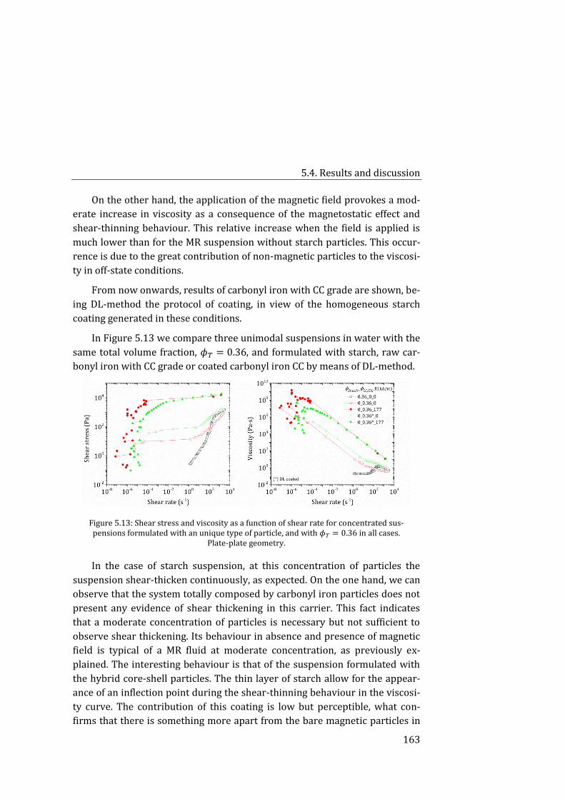
5.4. Results and discussion
163
On the other hand, the application of the magnetic field provokes a mod-
erate increase in viscosity as a consequence of the magnetostatic effect and
shear-thinning behaviour. This relative increase when the field is applied is
much lower than for the MR suspension without starch particles. This occur-
rence is due to the great contribution of non-magnetic particles to the viscosi-
ty in off-state conditions.
From now onwards, results of carbonyl iron with CC grade are shown, be-
ing DL-method the protocol of coating, in view of the homogeneous starch
coating generated in these conditions.
In Figure 5.13 we compare three unimodal suspensions in water with the
same total volume fraction, 𝜙𝑇 = 0.36, and formulated with starch, raw car-
bonyl iron with CC grade or coated carbonyl iron CC by means of DL-method.
Figure 5.13: Shear stress and viscosity as a function of shear rate for concentrated sus-pensions formulated with an unique type of particle, and with 𝜙𝑇 = 0.36 in all cases.
Plate-plate geometry.
In the case of starch suspension, at this concentration of particles the
suspension shear-thicken continuously, as expected. On the one hand, we can
observe that the system totally composed by carbonyl iron particles does not
present any evidence of shear thickening in this carrier. This fact indicates
that a moderate concentration of particles is necessary but not sufficient to
observe shear thickening. Its behaviour in absence and presence of magnetic
field is typical of a MR fluid at moderate concentration, as previously ex-
plained. The interesting behaviour is that of the suspension formulated with
the hybrid core-shell particles. The thin layer of starch allow for the appear-
ance of an inflection point during the shear-thinning behaviour in the viscosi-
ty curve. The contribution of this coating is low but perceptible, what con-
firms that there is something more apart from the bare magnetic particles in
5. Shear thickening in bimodal suspensions
164
the system. The suspensions of magnetic particles, well starch-coated or not,
are very similar in terms of particle size and sedimentation rates. The differ-
ence in viscosity curves in the absence of magnetic field can come from the
fact that the layer of starch results in particles with higher roughness. Thus, in
the core-shell suspension strong interactions between rough surfaces are tak-
ing place, in accordance with [63]. Apart from higher roughness, the shear-
induced particle network is reinforced by hydrogen bonding between termi-
nal hydroxyl groups from the layer of starch.
The coating in on-state field conditions mainly affects the rheogram at
low shear rates. The non-coated concentrated suspension displays a clear
yield stress while in the coated suspension the transition from low to inter-
mediate shear rates is moderate in terms of shear stresses, as a consequence
of a reduce magnetic particle-particle interaction.
Comparison between bimodal suspensions and formu-5.4.3.
lated with hybrid core-shell particles
In this subsection we revisit the experimental rheological results of concen-
trated suspensions in water formulated by combination of two elements:
starch and carbonyl iron. We consider unimodal and bimodal suspensions
with a 𝜙𝑇 ≥ 0.35, well formulated with hybrid magnetic-non magnetic core-
shell particles or with mixtures of these particles, respectively.
Figure 5.14 show the viscosity curves of these suspensions in absence
and presence of magnetic field. From these graphs we can summarize several
aspects. In the absence of magnetic field, suspensions with a 𝜙𝑆𝑡𝑎𝑟𝑐ℎ = 0.36
provide shear thickening whatever the magnetic concentration. The intensity
of this behaviour decreases as magnetic concentration increases, although the
viscosity is higher, due to a higher total concentration. The fact that magnetic
particles have a smoother particle surface compared to that of starch gran-
ules, may be the reason for this reduction. The shear-induced particle net-
work in the shear-thickening regime may flow easily when a portion of parti-
cles are smooth spheres.
However, the fact of having a 𝜙𝑇 = 0.36 does not guarantee the exhibi-
tion of ST. The magnetic unimodal suspensions at this concentration do not
display ST but a shear-thinning region in the entire range of shear rates eval-
uated. At low shear rates the viscosity of the magnetic suspensions is higher
than for starch suspensions. It can be explained due to the difference in parti-
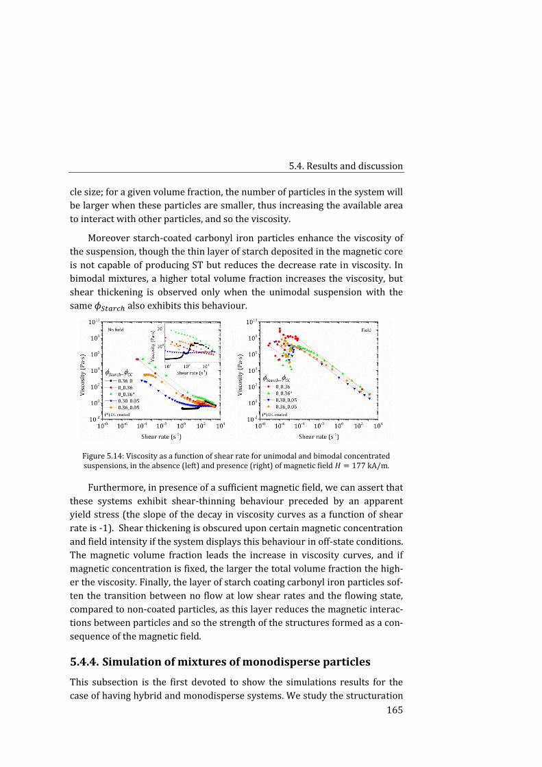
5.4. Results and discussion
165
cle size; for a given volume fraction, the number of particles in the system will
be larger when these particles are smaller, thus increasing the available area
to interact with other particles, and so the viscosity.
Moreover starch-coated carbonyl iron particles enhance the viscosity of
the suspension, though the thin layer of starch deposited in the magnetic core
is not capable of producing ST but reduces the decrease rate in viscosity. In
bimodal mixtures, a higher total volume fraction increases the viscosity, but
shear thickening is observed only when the unimodal suspension with the
same 𝜙𝑆𝑡𝑎𝑟𝑐ℎ also exhibits this behaviour.
Figure 5.14: Viscosity as a function of shear rate for unimodal and bimodal concentrated suspensions, in the absence (left) and presence (right) of magnetic field 𝐻 = 177 kA/m.
Furthermore, in presence of a sufficient magnetic field, we can assert that
these systems exhibit shear-thinning behaviour preceded by an apparent
yield stress (the slope of the decay in viscosity curves as a function of shear
rate is -1). Shear thickening is obscured upon certain magnetic concentration
and field intensity if the system displays this behaviour in off-state conditions.
The magnetic volume fraction leads the increase in viscosity curves, and if
magnetic concentration is fixed, the larger the total volume fraction the high-
er the viscosity. Finally, the layer of starch coating carbonyl iron particles sof-
ten the transition between no flow at low shear rates and the flowing state,
compared to non-coated particles, as this layer reduces the magnetic interac-
tions between particles and so the strength of the structures formed as a con-
sequence of the magnetic field.
Simulation of mixtures of monodisperse particles 5.4.4.
This subsection is the first devoted to show the simulations results for the
case of having hybrid and monodisperse systems. We study the structuration
5. Shear thickening in bimodal suspensions
166
of mixtures of magnetic and non-magnetic spherical particles subjected to an
external magnetic field, both at rest and under distinct values of shear rates.
The final objective is to determine whether the partial substitution of magnet-
ic particles by non-magnetic ones may enhance the yield stress in these simu-
lations, as it is found in experimental works. Moreover, we are interested in
the curves of the final rheogram, in relation to the possible appearance of
shear thickening in the systems with a higher particle concentration and in
the range of shear rates evaluated.
During structuration at rest, we followed the evolution of the total mag-
netic energy, the z-component of the magnetic moment and the average num-
ber of particles surrounding a given particle. In the start-up tests we payed
attention to the evolution of the dimensionless magnetic stress during the
simulation time, and the static magnetic stress was obtained from the peak of
this stress growth test. The total shear stress was then calculated as the sum
of this static magnetic stress and the hydrodynamic contribution from the
applied shear. For simplicity, other contributions to the shear stress coming
from the rest of non-hydrodynamic forces were neglected in comparison with
the magnetic contribution to the stress. With this, a rheogram was construct-
ed for each system considered, and its related yield stress was obtained.
It is noteworthy to point out that all these parameters exposed in this
subsection refer to dimensionless magnitudes, and are averaged over five
runs at least.
Structuration at rest
In the first step of the simulation code Equation 5.1 is employed to solve the
motion of particles, being the main contribution that coming from the exter-
nal magnetic field, and the fluid field velocity is null. In this sense, at rest, par-
ticle aggregation and structuration takes place. Only results for 𝜙𝑀′ = 1 and
𝜙𝑇 = 0.30 are shown in this part, as their behaviour is representative for the
rest of concentrations evaluated.
In Figure 5.15 we show the time evolution of the dimensionless total
magnetic energy for some bimodal mixtures investigated. As it was expected,
at the beginning of the simulation all systems share the same total magnetic
energy (null) as magnetic and non-magnetic particles are randomly distribut-
ed in the simulation box. The total magnetic energy continuously decreases
with time until each system reaches a plateau with small oscillations when it
stabilizes. It is noteworthy that the simulation time imposed in this step is
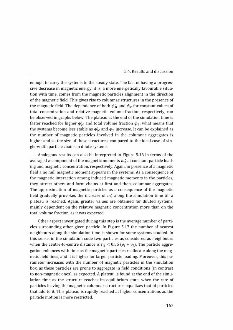
5.4. Results and discussion
167
enough to carry the systems to the steady state. The fact of having a progres-
sive decrease in magnetic energy, it is, a more energetically favourable situa-
tion with time, comes from the magnetic particles alignment in the direction
of the magnetic field. This gives rise to columnar structures in the presence of
the magnetic field. The dependence of both 𝜙𝑀′ and 𝜙𝑇 for constant values of
total concentration and relative magnetic volume fraction, respectively, can
be observed in graphs below. The plateau at the end of the simulation time is
faster reached for higher 𝜙𝑀′ and total volume fraction 𝜙𝑇 , what means that
the systems become less stable as 𝜙𝑀′ and 𝜙𝑇 increase. It can be explained as
the number of magnetic particles involved in the columnar aggregates is
higher and so the size of these structures, compared to the ideal case of sin-
gle-width particle chains in dilute systems.
Analogous results can also be interpreted in Figure 5.16 in terms of the
averaged 𝑧-component of the magnetic moments 𝑚𝑧∗ at constant particle load-
ing and magnetic concentration, respectively. Again, in presence of a magnetic
field a no null magnetic moment appears in the systems. As a consequence of
the magnetic interaction among induced magnetic moments in the particles,
they attract others and form chains at first and then, columnar aggregates.
The approximation of magnetic particles as a consequence of the magnetic
field gradually provokes the increase of 𝑚𝑧∗ along the simulation time till a
plateau is reached. Again, greater values are obtained for diluted systems,
mainly dependent on the relative magnetic concentration more than on the
total volume fraction, as it was expected.
Other aspect investigated during this step is the average number of parti-
cles surrounding other given particle. In Figure 5.17 the number of nearest
neighbours along the simulation time is shown for some systems studied. In
this sense, in the simulation code two particles as considered as neighbours
when the centre-to-centre distance is 𝑟𝑖𝑗 < 0.55 (𝜎𝑖 + 𝜎𝑗). The particle aggre-
gation enhances with time as the magnetic particles reallocate along the mag-
netic field lines, and it is higher for larger particle loading. Moreover, this pa-
rameter increases with the number of magnetic particles in the simulation
box, as these particles are prone to aggregate in field conditions (in contrast
to non-magnetic ones), as expected. A plateau is found at the end of the simu-
lation time as the structure reaches its equilibrium state, when the rate of
particles leaving the magnetic columnar structures equalizes that of particles
that add to it. This plateau is rapidly reached at higher concentrations as the
particle motion is more restricted.
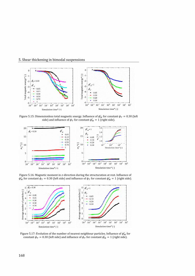
5. Shear thickening in bimodal suspensions
168
Figure 5.15: Dimensionless total magnetic energy. Influence of 𝜙𝑀′ for constant 𝜙𝑇 = 0.30 (left
side) and influence of 𝜙𝑇 for constant 𝜙𝑀′ = 1 (right side).
Figure 5.16: Magnetic moment in z-direction during the structuration at rest. Influence of 𝜙𝑀
′ for constant 𝜙𝑇 = 0.30 (left side) and influence of 𝜙𝑇 for constant 𝜙𝑀′ = 1 (right side).
Figure 5.17: Evolution of the number of nearest neighbour particles. Influence of 𝜙𝑀′ for
constant 𝜙𝑇 = 0.30 (left side) and influence of 𝜙𝑇 for constant 𝜙𝑀′ = 1 (right side).
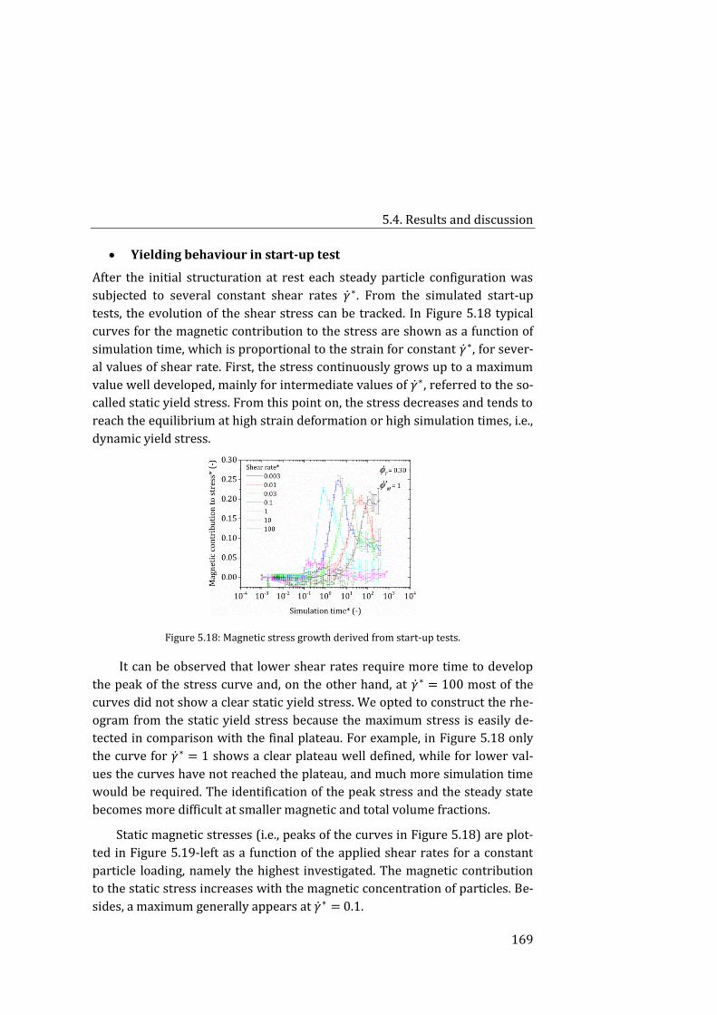
5.4. Results and discussion
169
Yielding behaviour in start-up test
After the initial structuration at rest each steady particle configuration was
subjected to several constant shear rates �̇�∗. From the simulated start-up
tests, the evolution of the shear stress can be tracked. In Figure 5.18 typical
curves for the magnetic contribution to the stress are shown as a function of
simulation time, which is proportional to the strain for constant �̇�∗, for sever-
al values of shear rate. First, the stress continuously grows up to a maximum
value well developed, mainly for intermediate values of �̇�∗, referred to the so-
called static yield stress. From this point on, the stress decreases and tends to
reach the equilibrium at high strain deformation or high simulation times, i.e.,
dynamic yield stress.
Figure 5.18: Magnetic stress growth derived from start-up tests.
It can be observed that lower shear rates require more time to develop
the peak of the stress curve and, on the other hand, at �̇�∗ = 100 most of the
curves did not show a clear static yield stress. We opted to construct the rhe-
ogram from the static yield stress because the maximum stress is easily de-
tected in comparison with the final plateau. For example, in Figure 5.18 only
the curve for �̇�∗ = 1 shows a clear plateau well defined, while for lower val-
ues the curves have not reached the plateau, and much more simulation time
would be required. The identification of the peak stress and the steady state
becomes more difficult at smaller magnetic and total volume fractions.
Static magnetic stresses (i.e., peaks of the curves in Figure 5.18) are plot-
ted in Figure 5.19-left as a function of the applied shear rates for a constant
particle loading, namely the highest investigated. The magnetic contribution
to the static stress increases with the magnetic concentration of particles. Be-
sides, a maximum generally appears at �̇�∗ = 0.1.
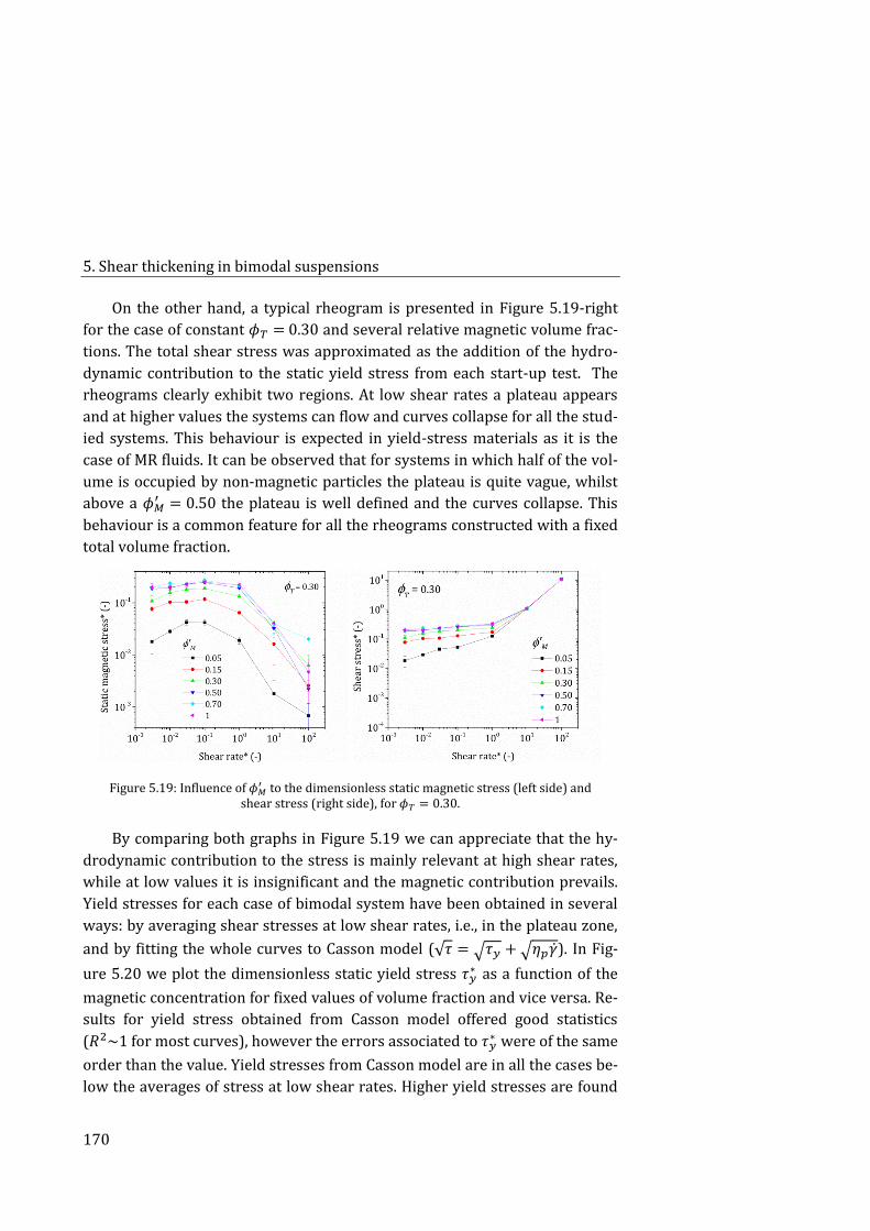
5. Shear thickening in bimodal suspensions
170
On the other hand, a typical rheogram is presented in Figure 5.19-right
for the case of constant 𝜙𝑇 = 0.30 and several relative magnetic volume frac-
tions. The total shear stress was approximated as the addition of the hydro-
dynamic contribution to the static yield stress from each start-up test. The
rheograms clearly exhibit two regions. At low shear rates a plateau appears
and at higher values the systems can flow and curves collapse for all the stud-
ied systems. This behaviour is expected in yield-stress materials as it is the
case of MR fluids. It can be observed that for systems in which half of the vol-
ume is occupied by non-magnetic particles the plateau is quite vague, whilst
above a 𝜙𝑀′ = 0.50 the plateau is well defined and the curves collapse. This
behaviour is a common feature for all the rheograms constructed with a fixed
total volume fraction.
Figure 5.19: Influence of 𝜙𝑀′ to the dimensionless static magnetic stress (left side) and
shear stress (right side), for 𝜙𝑇 = 0.30.
By comparing both graphs in Figure 5.19 we can appreciate that the hy-
drodynamic contribution to the stress is mainly relevant at high shear rates,
while at low values it is insignificant and the magnetic contribution prevails.
Yield stresses for each case of bimodal system have been obtained in several
ways: by averaging shear stresses at low shear rates, i.e., in the plateau zone,
and by fitting the whole curves to Casson model (√𝜏 = √𝜏𝑦 + √휂𝑝�̇�). In Fig-
ure 5.20 we plot the dimensionless static yield stress 𝜏𝑦∗ as a function of the
magnetic concentration for fixed values of volume fraction and vice versa. Re-
sults for yield stress obtained from Casson model offered good statistics
(𝑅2~1 for most curves), however the errors associated to 𝜏𝑦∗ were of the same
order than the value. Yield stresses from Casson model are in all the cases be-
low the averages of stress at low shear rates. Higher yield stresses are found
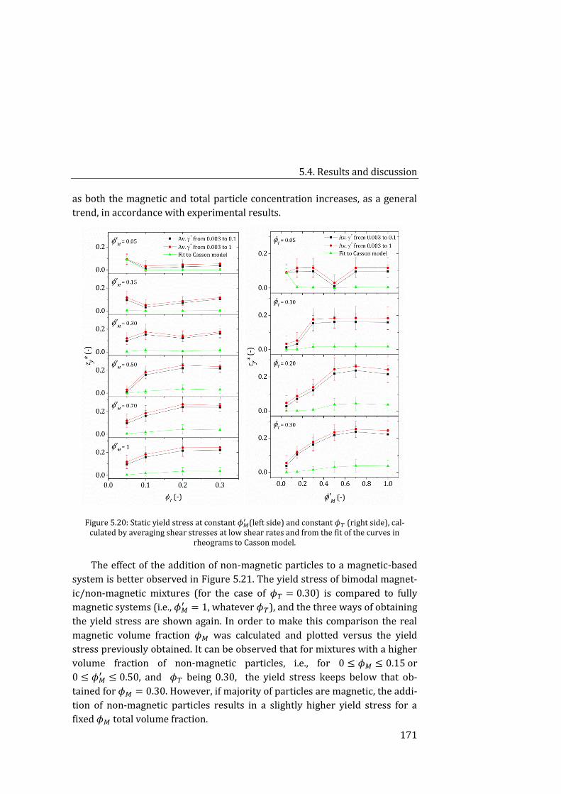
5.4. Results and discussion
171
as both the magnetic and total particle concentration increases, as a general
trend, in accordance with experimental results.
Figure 5.20: Static yield stress at constant 𝜙𝑀′ (left side) and constant 𝜙𝑇 (right side), cal-
culated by averaging shear stresses at low shear rates and from the fit of the curves in rheograms to Casson model.
The effect of the addition of non-magnetic particles to a magnetic-based
system is better observed in Figure 5.21. The yield stress of bimodal magnet-
ic/non-magnetic mixtures (for the case of 𝜙𝑇 = 0.30) is compared to fully
magnetic systems (i.e., 𝜙𝑀′ = 1, whatever 𝜙𝑇), and the three ways of obtaining
the yield stress are shown again. In order to make this comparison the real
magnetic volume fraction 𝜙𝑀 was calculated and plotted versus the yield
stress previously obtained. It can be observed that for mixtures with a higher
volume fraction of non-magnetic particles, i.e., for 0 ≤ 𝜙𝑀 ≤ 0.15 or
0 ≤ 𝜙𝑀′ ≤ 0.50, and 𝜙𝑇 being 0.30, the yield stress keeps below that ob-
tained for 𝜙𝑀 = 0.30. However, if majority of particles are magnetic, the addi-
tion of non-magnetic particles results in a slightly higher yield stress for a
fixed 𝜙𝑀 total volume fraction.
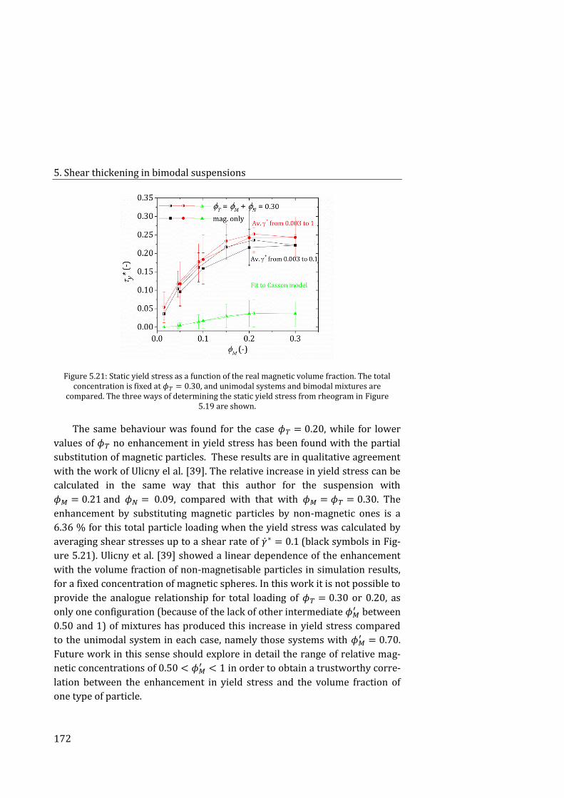
5. Shear thickening in bimodal suspensions
172
Figure 5.21: Static yield stress as a function of the real magnetic volume fraction. The total concentration is fixed at 𝜙𝑇 = 0.30, and unimodal systems and bimodal mixtures are
compared. The three ways of determining the static yield stress from rheogram in Figure 5.19 are shown.
The same behaviour was found for the case 𝜙𝑇 = 0.20, while for lower
values of 𝜙𝑇 no enhancement in yield stress has been found with the partial
substitution of magnetic particles. These results are in qualitative agreement
with the work of Ulicny el al. [39]. The relative increase in yield stress can be
calculated in the same way that this author for the suspension with
𝜙𝑀 = 0.21 and 𝜙𝑁 = 0.09, compared with that with 𝜙𝑀 = 𝜙𝑇 = 0.30. The
enhancement by substituting magnetic particles by non-magnetic ones is a
6.36 % for this total particle loading when the yield stress was calculated by
averaging shear stresses up to a shear rate of �̇�∗ = 0.1 (black symbols in Fig-
ure 5.21). Ulicny et al. [39] showed a linear dependence of the enhancement
with the volume fraction of non-magnetisable particles in simulation results,
for a fixed concentration of magnetic spheres. In this work it is not possible to
provide the analogue relationship for total loading of 𝜙𝑇 = 0.30 or 0.20, as
only one configuration (because of the lack of other intermediate 𝜙𝑀′ between
0.50 and 1) of mixtures has produced this increase in yield stress compared
to the unimodal system in each case, namely those systems with 𝜙𝑀′ = 0.70.
Future work in this sense should explore in detail the range of relative mag-
netic concentrations of 0.50 < 𝜙𝑀′ < 1 in order to obtain a trustworthy corre-
lation between the enhancement in yield stress and the volume fraction of
one type of particle.
5.4. Results and discussion
173
Simulation of mixtures of polydisperse particles 5.4.5.
The rheological behaviour of MRST fluids was experimentally studied in pre-
vious subsections. From these results it was concluded that it is possible for
these hybrid systems to show both magnetic and shear-thickening responses
if the concentration of magnetic particles or the field intensity were kept low
enough. Moreover, shear-thickening behaviour requires large concentrations
of particles to occur.
Although monodisperse particles were used in Subsection 5.4.4., and
these simulations agree with other authors that found a beneficial effect in
the yield stress when substituting part of magnetic particles by non-magnetic
ones, the second objective of observing the shear-thickening response in the
constructed rheograms was not achieved. It is due to the maximum total vol-
ume fraction that could be allocated in the simulation box with monodisperse
particles was 𝜙𝑇 = 0.30. With this intention in mind higher total volume frac-
tions are necessary, so that we performed new simulations of mixtures of par-
ticles in which both populations present polydispersity.
These simulations follow the same procedure that in the monodisperse
case, i.e., structuration at rest and under constant shear flows, being the sys-
tems subjected to a constant external magnetic field in both steps. Although
some results of intermediate steps are shown in this subsection, the final rhe-
ograms will be the focus of our attention. From now on, rheograms presented
here are constructed by adding the hydrodynamic contribution to the total
static stress, which accounts for magnetic, repulsive, wall and Brownian in-
teractions. This is in contrast to Subsection 5.4.4., where only the magnetic
contribution was taken into account in the static stress, as it was by far the
main contribution to the total stress. The incorporation of polydispersity is
firstly studied in bimodal systems, and then in the unimodal case, for which
𝜙𝑁 = 0.
Bimodal case
In these simulations non-magnetic volume fractions are studied in the inter-
val 𝜙𝑁 = 0.30 − 0.50, while magnetic volume fractions used are very low, in
the range from 𝜙𝑀 = 0.0002 to 0.0005. These values have been chosen below
the experimental magnetic volume fractions in order not to obscure the ap-
pearance of shear thickening. Regarding the magnetic field intensity the mix-
tures are subjected to, we consider the case of the value employed in experi-
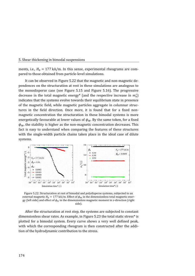
5. Shear thickening in bimodal suspensions
174
ments, i.e., 𝐻0 = 177 kA/m. In this sense, experimental rheograms are com-
pared to those obtained from particle-level simulations.
It can be observed in Figure 5.22 that the magnetic and non-magnetic de-
pendences on the structuration at rest in these simulations are analogous to
the monodisperse case (see Figure 5.15 and Figure 5.16). The progressive
decrease in the total magnetic energy* (and the respective increase in 𝑚𝑧∗)
indicates that the systems evolve towards their equilibrium state in presence
of the magnetic field, while magnetic particles aggregate in columnar struc-
tures in the field direction. Once more, it is found that for a fixed non-
magnetic concentration the structuration in these bimodal systems is more
energetically favourable at lower values of 𝜙𝑀. By the same token, for a fixed
𝜙𝑀, the stability is higher as the non-magnetic concentration decreases. This
fact is easy to understand when comparing the features of these structures
with the single-width particle chains taken place in the ideal case of dilute
systems.
Figure 5.22: Structuration at rest of bimodal and polydisperse systems, subjected to an external magnetic 𝐻0 = 177 kA/m. Effect of 𝜙𝑀 in the dimensionless total magnetic ener-gy (left side) and effect of 𝜙𝑁 in the dimensionless magnetic moment in z-direction (right
side).
After the structuration at rest step, the systems are subjected to constant
dimensionless shear rates. As example, in Figure 5.23 the total static stress* is
plotted for a bimodal system. Every curve shows a very well defined peak,
with which the corresponding rheogram is then constructed after the addi-
tion of the hydrodynamic contribution to the stress.
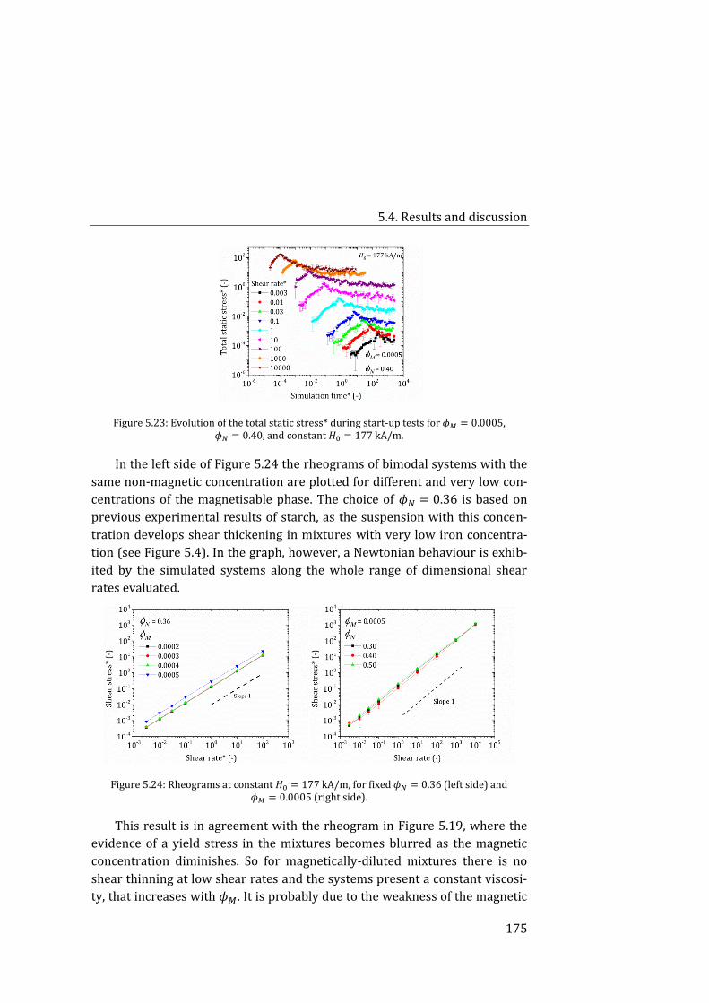
5.4. Results and discussion
175
Figure 5.23: Evolution of the total static stress* during start-up tests for 𝜙𝑀 = 0.0005, 𝜙𝑁 = 0.40, and constant 𝐻0 = 177 kA/m.
In the left side of Figure 5.24 the rheograms of bimodal systems with the
same non-magnetic concentration are plotted for different and very low con-
centrations of the magnetisable phase. The choice of 𝜙𝑁 = 0.36 is based on
previous experimental results of starch, as the suspension with this concen-
tration develops shear thickening in mixtures with very low iron concentra-
tion (see Figure 5.4). In the graph, however, a Newtonian behaviour is exhib-
ited by the simulated systems along the whole range of dimensional shear
rates evaluated.
Figure 5.24: Rheograms at constant 𝐻0 = 177 kA/m, for fixed 𝜙𝑁 = 0.36 (left side) and 𝜙𝑀 = 0.0005 (right side).
This result is in agreement with the rheogram in Figure 5.19, where the
evidence of a yield stress in the mixtures becomes blurred as the magnetic
concentration diminishes. So for magnetically-diluted mixtures there is no
shear thinning at low shear rates and the systems present a constant viscosi-
ty, that increases with 𝜙𝑀. It is probably due to the weakness of the magnetic
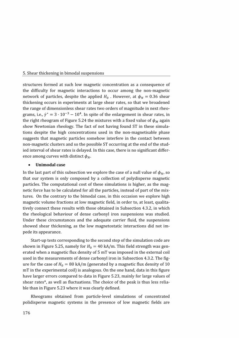
5. Shear thickening in bimodal suspensions
176
structures formed at such low magnetic concentration as a consequence of
the difficulty for magnetic interactions to occur among the non-magnetic
network of particles, despite the applied 𝐻0 . However, at 𝜙𝑁 = 0.36 shear
thickening occurs in experiments at large shear rates, so that we broadened
the range of dimensionless shear rates two orders of magnitude in next rheo-
grams, i.e., �̇�∗ = 3 · 10−3 − 104. In spite of the enlargement in shear rates, in
the right rheogram of Figure 5.24 the mixtures with a fixed value of 𝜙𝑀 again
show Newtonian rheology. The fact of not having found ST in these simula-
tions despite the high concentrations used in the non-magnetisable phase
suggests that magnetic particles somehow interfere in the contact between
non-magnetic clusters and so the possible ST occurring at the end of the stud-
ied interval of shear rates is delayed. In this case, there is no significant differ-
ence among curves with distinct 𝜙𝑁.
Unimodal case
In the last part of this subsection we explore the case of a null value of 𝜙𝑁, so
that our system is only composed by a collection of polydisperse magnetic
particles. The computational cost of these simulations is higher, as the mag-
netic force has to be calculated for all the particles, instead of part of the mix-
tures. On the contrary to the bimodal case, in this occasion we explore high
magnetic volume fractions at low magnetic field, in order to, at least, qualita-
tively connect these results with those obtained in Subsection 4.3.2, in which
the rheological behaviour of dense carbonyl iron suspensions was studied.
Under these circumstances and the adequate carrier fluid, the suspensions
showed shear thickening, as the low magnetostatic interactions did not im-
pede its appearance.
Start-up tests corresponding to the second step of the simulation code are
shown in Figure 5.25, namely for 𝐻0 = 40 kA/m. This field strength was gen-
erated when a magnetic flux density of 5 mT was imposed in the external coil
used in the measurements of dense carbonyl iron in Subsection 4.3.2. The fig-
ure for the case of 𝐻0 = 80 kA/m (generated by a magnetic flux density of 10
mT in the experimental coil) is analogous. On the one hand, data in this figure
have larger errors compared to data in Figure 5.23, mainly for large values of
shear rates*, as well as fluctuations. The choice of the peak is thus less relia-
ble than in Figure 5.23 where it was clearly defined.
Rheograms obtained from particle-level simulations of concentrated
polidisperse magnetic systems in the presence of low magnetic fields are
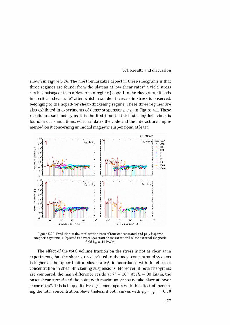
5.4. Results and discussion
177
shown in Figure 5.26. The most remarkable aspect in these rheograms is that
three regimes are found: from the plateau at low shear rates* a yield stress
can be envisaged; then a Newtonian regime (slope 1 in the rheogram); it ends
in a critical shear rate* after which a sudden increase in stress is observed,
belonging to the hoped-for shear-thickening regime. These three regimes are
also exhibited in experiments of dense suspensions, e.g., in Figure 4.1. These
results are satisfactory as it is the first time that this striking behaviour is
found in our simulations, what validates the code and the interactions imple-
mented on it concerning unimodal magnetic suspensions, at least.
Figure 5.25: Evolution of the total static stress of four concentrated and polydisperse magnetic systems, subjected to several constant shear rates* and a low external magnetic
field 𝐻0 = 40 kA/m.
The effect of the total volume fraction on the stress is not as clear as in
experiments, but the shear stress* related to the most concentrated systems
is higher at the upper limit of shear rates*, in accordance with the effect of
concentration in shear-thickening suspensions. Moreover, if both rheograms
are compared, the main difference reside at �̇�∗ = 103. At 𝐻0 = 80 kA/m, the
onset shear stress* and the point with maximum viscosity take place at lower
shear rates*. This is in qualitative agreement again with the effect of increas-
ing the total concentration. Nevertheless, if both curves with 𝜙𝑁 = 𝜙𝑇 = 0.50
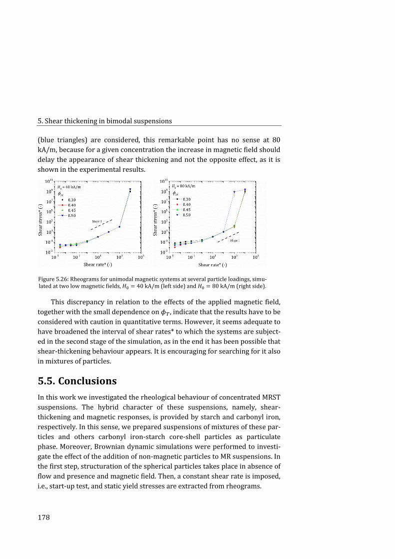
5. Shear thickening in bimodal suspensions
178
(blue triangles) are considered, this remarkable point has no sense at 80
kA/m, because for a given concentration the increase in magnetic field should
delay the appearance of shear thickening and not the opposite effect, as it is
shown in the experimental results.
Figure 5.26: Rheograms for unimodal magnetic systems at several particle loadings, simu-lated at two low magnetic fields, 𝐻0 = 40 kA/m (left side) and 𝐻0 = 80 kA/m (right side).
This discrepancy in relation to the effects of the applied magnetic field,
together with the small dependence on 𝜙𝑇 , indicate that the results have to be
considered with caution in quantitative terms. However, it seems adequate to
have broadened the interval of shear rates* to which the systems are subject-
ed in the second stage of the simulation, as in the end it has been possible that
shear-thickening behaviour appears. It is encouraging for searching for it also
in mixtures of particles.
Conclusions 5.5.
In this work we investigated the rheological behaviour of concentrated MRST
suspensions. The hybrid character of these suspensions, namely, shear-
thickening and magnetic responses, is provided by starch and carbonyl iron,
respectively. In this sense, we prepared suspensions of mixtures of these par-
ticles and others carbonyl iron-starch core-shell particles as particulate
phase. Moreover, Brownian dynamic simulations were performed to investi-
gate the effect of the addition of non-magnetic particles to MR suspensions. In
the first step, structuration of the spherical particles takes place in absence of
flow and presence and magnetic field. Then, a constant shear rate is imposed,
i.e., start-up test, and static yield stresses are extracted from rheograms.
5.5. Conclusions
179
The inclusion of attractive interparticle interactions, through the addition
of magnetic particles, in a shear-thickening system progressively delays this
phenomenon and reduces the relative increase of viscosity. In absence of
magnetic field carbonyl iron particles enhance the viscosity in the entire
range of shear stresses as the total concentration increases. In on-state condi-
tions magnetostatic interactions prevails at low shear rates, so that the sus-
pensions show shear-thinning, that may be preceded by an apparent yield
stress under certain conditions. This behaviour can exist in the whole viscosi-
ty curve if the magnetic particle concentration or field intensity are high
enough to completely weaken or inhibit the shear-thickening behaviour
found in absence of magnetic field. In this sense, a drastic reduction in the
slope of shear thickening is found for increasing magnetic fields when the
magnetic volume fraction is above a critical value of 0.001. Furthermore,
there is a significant effect of magnetic field in the minimum value of 𝑁1,
which is coincident to the yield stress, however this field dependence is not
clear in relation to the crossover stress.
Regarding core-shell particles, several methods of coating were em-
ployed, and some of them provided a homogeneous layer of starch onto car-
bonyl iron particles. At moderate concentration, 𝜙𝑇 = 0.36, coated particles
increase the viscosity compared to non-coated ones, probably due to certain
roughness from starch coating, that also contribute to hydrogen bonds within
shear-induced particle networks. Under field conditions, the effect of the thin
layer of starch is mainly appreciated at low shear rates, as the suspension
gradually changes its viscosity, instead of showing a clear yield stress, which
is the case of the analogue suspension with raw magnetic particles.
The simulation code adequately corroborates the formation of field-
induced columnar aggregates that break during shear. As expected, a higher
total and magnetic volume fraction produces thicker structures that result in
a less favourable energy state if compared with the ideal diluted suspensions
where single-width chains are formed. Regarding the second stage, a wide
range of dimensionless shear rates was used in the growth tests to construct
the rheograms. The initial plateau at low shear rates supports experimental
results of magnetorheological suspensions, and the yield stress grows with
both magnetic and total concentration. In agreement with other authors, an
enhancement in yield stress is found when magnetic particles are partially
substituted by non-magnetic ones in this type of fluids, for 𝜙𝑇 = 0.20 and
0.30. However, there is no evidence of shear thickening when considering
5. Shear thickening in bimodal suspensions
180
these total concentrations in monodisperse mixtures (the maximum achieva-
ble is 𝜙𝑇 = 0.30), whatever the ratio of magnetic and non-magnetic volume
fractions used, in agreement with experimental results up to this value.
The incorporation of certain polydispersity and different mean diameters
for each population of particles enhances the total volume fraction in the sim-
ulation box and so it allows a more realistic approach to the rheological be-
haviour of these dense systems. As a consequence, shear-thickening behav-
iour finally appeared in the simulations of dense systems formulated only
with magnetisable particles. However, this viscosity enhancement has not
been observed yet in our bimodal systems with similar values of volume frac-
tions and external field compared to the experiments, probably conditioned
by an insufficient limit in the upper shear rate evaluated in the second stage
of the simulation code through the growth tests.
In summary, the rheological behaviour of concentrated MRST suspen-
sions can be easily tuned by modifying the elements of the suspension. On the
one hand, by minimizing particle-fluid chemical and physical interactions, the
colloidal suspension stabilizes and shear thickening may be observed under
adequate circumstances. On the other hand, the connection between friction
at higher concentrations and particle surface features is clear. In this sense,
particles can be tailored in type, size, shape, deformability and roughness to
control the appearance of shear thickening and its strength.
References 5.6.
[1] Stickel J J and Powell R L 2005 Fluid mechanics and rheology of dense suspensions Annu. Rev. Fluid Mech. 37 129–149
[2] Mewis J and Wagner N J 2009 Current trends in suspension rheol-ogy J. Non-Newton. Fluid Mech. 157 147–50
[3] Denn M M and Morris J F 2014 Rheology of non-Brownian suspen-sions Annu. Rev. Chem. Biomol. Eng. 5 203–228
[4] Tanner R I 2018 Review Article: Aspects of non-colloidal suspen-sion rheology Phys. Fluids 30 101301
[5] Gallier S, Lemaire E, Peters F and Lobry L 2014 Rheology of sheared suspensions of rough frictional particles J. Fluid Mech. 757 514–549
5.6. References
181
[6] Rastogi S R, Wagner N J and Lustig S R 1996 Microstructure and rhe-ology of polydisperse, charged suspensions J. Chem. Phys. 104 9249–9258
[7] van der Vaart K, Rahmani Y, Zargar R, Hu Z, Bonn D and Schall P 2013 Rheology of concentrated soft and hard-sphere suspensions J. Rheol. 57 1195–209
[8] Galindo-Rosales F 2016 Complex fluids in energy dissipating systems Appl. Sci. 6 206
[9] Wagner N J and Brady J F 2009 Shear thickening in colloidal disper-sions Phys. Today 62 27–32
[10] Denn M M, Morris J F and Bonn D 2018 Shear thickening in concen-trated suspensions of smooth spheres in Newtonian suspending fluids Soft Matter 14 170–184
[11] Metzner A B and Whitlock M 1958 Flow behavior of concentrated (di-latant) suspensions Trans. Soc. Rheol. 2 239–54
[12] Hoffman R L 1972 Discontinuous and dilatant viscosity behavior in concentrated suspensions. I. Observation of a flow instability Trans. Soc. Rhe-ol. 16 155–173
[13] Hoffman R L 1974 Discontinuous and dilatant viscosity behavior in concentrated suspensions. II. Theory and experimental tests J. Colloid Inter-face Sci. 46 491–506
[14] Brady J F and Bossis G 1985 The rheology of concentrated suspen-sions of spheres in simple shear flow by numerical simulation J. Fluid Mech. 155 105
[15] Maranzano B J and Wagner N J 2001 The effects of particle size on re-versible shear thickening of concentrated colloidal dispersions J. Chem. Phys. 114 10514–27
[16] Seto R, Mari R, Morris J F and Denn M M 2013 Discontinuous shear thickening of frictional hard-sphere suspensions Phys. Rev. Lett. 111
[17] Fernandez N, Mani R, Rinaldi D, Kadau D, Mosquet M, Lombois-Burger H, Cayer-Barrioz J, Herrmann H J, Spencer N D and Isa L 2013 Micro-scopic mechanism for shear thickening of non-Brownian suspensions Phys. Rev. Lett. 111
[18] Mari R, Seto R, Morris J F and Denn M M 2014 Shear thickening, fric-tionless and frictional rheologies in non-Brownian suspensions J. Rheol. 58 1693–1724
5. Shear thickening in bimodal suspensions
182
[19] Lin N Y C, Guy B M, Hermes M, Ness C, Sun J, Poon W C K and Cohen I 2015 Hydrodynamic and contact contributions to continuous shear thick-ening in colloidal suspensions Phys. Rev. Lett. 115
[20] Clavaud C, Bérut A, Metzger B and Forterre Y 2017 Revealing the frictional transition in shear-thickening suspensions Proc. Natl. Acad. Sci. 114 5147–5152
[21] Barnes H A 1989 Shear-thickening (“Dilatancy”) in suspensions of nonaggregating solid particles dispersed in Newtonian liquids J. Rheol. 33 329–366
[22] Frith W J, d’Haene P, Buscall R and Mewis J 1996 Shear thickening in model suspensions of sterically stabilized particles J. Rheol. 40 531–548
[23] Egres R G and Wagner N J 2005 The rheology and microstructure of acicular precipitated calcium carbonate colloidal suspensions through the shear thickening transition J. Rheol. 49 719–746
[24] Lootens D, Damme H van, Hémar Y and Hébraud P 2005 Dilatant flow of concentrated suspensions of rough particles Phys. Rev. Lett. 95
[25] Lin N Y C, Ness C, Cates M E, Sun J and Cohen I 2016 Tunable shear thickening in suspensions Proc. Natl. Acad. Sci. 113 10774–10778
[26] Brown E, Forman N A, Orellana C S, Zhang H, Maynor B W, Betts D E, Desimone J M and Jaeger H M 2010 Generality of shear thickening in dense suspensions Nat. Mater. 9 1–5
[27] de Vicente J, Klingenberg D J and Hidalgo-Álvarez R 2011 Magne-torheological fluids: a review Soft Matter 7 3701
[28] James N M, Xue H, Goyal M and Jaeger H M 2019 Controlling shear jamming in dense suspensions via the particle aspect ratio Soft Matter 15 3649–54
[29] Brown E, Zhang H, Forman N A, Maynor B W, Betts D E, DeSimone J M and Jaeger H M 2011 Shear thickening and jamming in densely packed suspensions of different particle shapes Phys. Rev. E 84
[30] Hsiao L C and Pradeep S 2019 Experimental synthesis and charac-terization of rough particles for colloidal and granular rheology Curr. Opin. Colloid Interface Sci. 43 94–112
[31] Guy B M, Hermes M and Poon W C K 2015 Towards a unified de-scription of the rheology of hard-particle suspensions Phys. Rev. Lett. 115
[32] Pednekar S, Chun J and Morris J F 2018 Bidisperse and polydisperse suspension rheology at large solid fraction J. Rheol. 62 513–526
5.6. References
183
[33] Krishnamurthy L-N, Wagner N J and Mewis J 2005 Shear thickening in polymer stabilized colloidal dispersions J. Rheol. 49 1347–1360
[34] James N M, Han E, de la Cruz R A L, Jureller J and Jaeger H M 2018 In-terparticle hydrogen bonding can elicit shear jamming in dense suspensions Nat. Mater. 17 965–70
[35] Chen Y, Zhou Y, Pi H and Zeng G 2019 Controlling the shear thicken-ing behavior of suspensions by changing the surface properties of dispersed microspheres RSC Adv. 9 3469–78
[36] Ghosh A, Chauhan I, Majumdar A and Butola B S 2017 Influence of cel-lulose nanofibers on the rheological behavior of silica-based shear-thickening fluid Cellulose 24 4163–71
[37] Tan Z, Ge J, Zhang H, Zhai P and Li W 2017 Dynamic response of shear thickening fluid reinforced with SiC nanowires under high strain rates Appl. Phys. Lett. 111 031902
[38] Madraki Y, Hormozi S, Ovarlez G, Guazzelli É and Pouliquen O 2017 Enhancing shear thickening Phys. Rev. Fluids 2
[39] Ulicny J C, Snavely K S, Golden M A and Klingenberg D J 2010 Enhanc-ing magnetorheology with nonmagnetizable particles Appl. Phys. Lett. 96 1–4
[40] Bombard A J F, Gonçalves F R, Morillas J R and Vicente J de 2014 Magnetorheology of dimorphic magnetorheological fluids based on nano-fibers Smart Mater. Struct. 23 125013
[41] Boczkowska A and Awietj S 2012 Microstructure and Properties of Magnetorheological Elastomers Advanced Elastomers - Technology, Properties and Applications ed A Boczkowska (InTech)
[42] Wilson B T and Klingenberg D J 2016 Effects of nonmagnetizable par-ticles on the structure of magnetorheological fluids Curr. Smart Mater. 1 35–48
[43] Li W H and Zhang X Z 2008 Rheology of magnetorheological shear thickening fluids Adv. Mater. Res. 32 161–4
[44] Zhang X, Li W and Gong X L 2008 Study on magnetorheological shear thickening fluid Smart Mater. Struct. 17 015051
[45] Tian Y, Jiang J, Meng Y and Wen S 2010 A shear thickening phenome-non in magnetic field controlled-dipolar suspensions Appl. Phys. Lett. 97 151904
[46] Lu A-H, Salabas E L and Schüth F 2007 Magnetic nanoparticles: syn-thesis, protection, functionalization, and application Angew. Chem. Int. Ed. 46 1222–44
5. Shear thickening in bimodal suspensions
184
[47] Bruncková H, Kabátová M and Dudrová E 2009 The effect of iron phosphate, alumina and silica coatings on the morphology of carbonyl iron particles Surf. Interface Anal.
[48] Malecki P, Kolman K, Piglowski J, Kaleta J and Krzak J 2015 Sol-gel method as a way of carbonyl iron powder surface modification for interac-tion improvement J. Solid State Chem. 226 224–30
[49] Wang S, Tang J, Zhao H, Wan J and Chen K 2014 Synthesis of mag-netite–silica core–shell nanoparticles via direct silicon oxidation J. Colloid Interface Sci. 432 43–46
[50] Narita A, Naka K and Chujo Y 2009 Facile control of silica shell layer thickness on hydrophilic iron oxide nanoparticles via reverse micelle meth-od Colloids Surf. Physicochem. Eng. Asp. 336 46–56
[51] Liu Q, Zhang Y and Laskowski J S 2000 The adsorption of polysac-charides onto mineral surfaces: an acid/base interaction Int. J. Miner. Pro-cess. 60 229–45
[52] Laskowski J S, Liu Q and O\textquotesingleConnor C T 2007 Current understanding of the mechanism of polysaccharide adsorption at the min-eral/aqueous solution interface Int. J. Miner. Process. 84 59–68
[53] Ma X 2008 Role of solvation energy in starch adsorption on oxide surfaces Colloids Surf. Physicochem. Eng. Asp. 320 36–42
[54] Dung T T, Danh T M, Hoa L T M, Chien D M and Duc N H 2009 Struc-tural and magnetic properties of starch-coated magnetite nanoparticles J. Exp. Nanosci. 4 259–267
[55] Subramanian S and Natarajan K A 1989 Adsorption behaviour of an oxidised starch onto haematite in the presence of calcium Miner. Eng. 2 55–64
[56] Jiang J-S, Gan Z-F, Yang Y, Du B, Qian M and Zhang P 2008 A novel magnetic fluid based on starch-coated magnetite nanoparticles functional-ized with homing peptide J. Nanoparticle Res. 11 1321–1330
[57] Lawless B D and Williams J 1993 Carbonyl iron particles in magnet-ic cell sorting Sep. Sci. Technol. 28 1939–45
[58] Sim H H, Kwon S H and Choi H J 2012 Xanthan gum-coated soft magnetic carbonyl iron composite particles and their magnetorheology Col-loid Polym. Sci. 291 963–969
[59] Vereda F, Segovia-Gutiérrez J P, Vicente J de and Hidalgo-Álvarez R 2014 Particle roughness in magnetorheology: effect on the strength of the field-induced structures J. Phys. Appl. Phys. 48 015309
5.6. References
185
[60] Fernández-Toledano J C, Ruiz-López J A, Hidalgo-Álvarez R and de Vi-cente J 2015 Simulations of polydisperse magnetorheological fluids: A struc-tural and kinetic investigation J. Rheol. 59 475–98
[61] López-López M T, Kuzhir P, Durán J D G and Bossis G 2010 Normal stresses in a shear flow of magnetorheological suspensions: Viscoelastic ver-sus Maxwell stresses J. Rheol. 54 1119–36
[62] de Vicente J, González-Caballero F, Bossis G and Volkova O 2002 Normal force study in concentrated carbonyl iron magnetorheological sus-pensions J. Rheol. 46 1295–303
[63] Hsu C-P, Ramakrishna S N, Zanini M, Spencer N D and Isa L 2018 Roughness-dependent tribology effects on discontinuous shear thickening Proc. Natl. Acad. Sci. 1–6

187
6. Isoviscous elastohydrodynamic
lubrication of inelastic
non-Newtonian fluids
K. Shahrivar, E.M. Ortigosa-Moya, R. Hidalgo-Álvarez, J. de Vicente
The content of this chapter is published in: Tribology International,
2019, 140, 105707.
https://doi.org/10.1016/j.triboint.2019.03.065
Abstract
We simulate the thin-film and frictional properties of shear-thinning and
shear-thickening fluids in the isoviscous elastohydrodynamic (I-EHL) regime
in point contacts. A double-Newtonian Carreau-Yasuda viscosity model is
employed to incorporate the shear rate dependence of the viscosity. Regres-
sion formulas for the film thickness and friction coefficient are proposed for
both non-Newtonian fluids. A master curve is proposed by using the product
between the entrainment speed and the effective viscosity in the contact.
Numerical results are satisfactorily compared with experimental data in xan-
tham gum solutions and fumed silica suspensions in the form of Stribeck
curves.
6. IEHL of inelastic non-Newtonian fluids
188
6.1. Introduction
The understanding of the tribological properties of inelastic non-Newtonian
fluids in compliant isoviscous elastohydrodynamic lubrication (I-EHL) is a hot
topic today [1–4]. On the one hand, inelastic non-Newtonian fluids are purely
dissipative fluids with a shear rate dependent viscosity. On the other hand,
the I-EHL occurs when either the tribopair has a small-reduced elastic modu-
lus or the lubricant has a very low pressure-viscosity index [5]. In the I-EHL
regime the pressure is high enough to cause elastic deformation but not suffi-
cient to produce a substantial change in viscosity.
Many biotribological contacts operate in the I-EHL. Some examples con-
cern the microcirculation of red blood cells in capillaries, blinking of eyes,
contact lenses, respiratory motion between pleural surfaces, synovial joints
and food products in mouth [4,6]. On the one hand, biological lubricants ex-
hibit non-Newtonian characteristics. Blood is an example that shows a strong
shear-thinning behaviour at the physiological concentration of 50 % red
blood cells. On the other hand, biological bearing surfaces often involve com-
plex structures and large deformations. These characteristics in compliant
biological tissues are responsible for the major contribution of fluid film ac-
tion to the lubrication at both tissue and cellular levels [7].
Reynolds presented the differential equation that governs the pressure
distribution in the full-film lubrication regime in his classical paper in 1886
[8]. Reynolds neglected inertia and gravitational effects in relation to viscous
action, and the analysis was restricted to an isoviscous and incompressible
fluid. Since then, many researchers tried to explain the full-film lubrication in
gears and mechanical components based on Reynolds theory, however, with
little success. In 1949, Grubin [9] incorporated the pressure-viscosity coeffi-
cient of the lubricant and the elastic deformation of the surfaces in the analy-
sis. This work resulted in the emergence of the EHL theory. Using numerical
calculations, Dowson and Higginson [10,11] developed a regression formula
for the prediction of the film thickness in line contacts. The most widely used
film thickness formula that is currently employed in EHL was introduced by
Hamrock and Dowson [12,13] for oil lubrication in circular contacts. Later
researchers further improved the method and extended the operating condi-
tions range, in particular, to achieve higher loads [14]. In 1987, Lubrecht [15]
introduced multilevel techniques. With this methodology it was possible to
numerically solve the partial differential equations at a lower computational
6.1. Introduction
189
cost with very dense meshes. Nijenbanning et al. [16] developed new film
thickness equations using this technique. More recently, Venner and Lubrecht
wrote a comprehensive book on this topic [17].
With regards to the friction characteristics, major efforts in developing
EHL theory were devoted in the past to study the full-film lubrication behav-
iour of Newtonian fluids despite the fact that there are many applications
where the lubricant is non-Newtonian. Hooke [18] and Ehret et al. [19] pro-
posed approximate methods to describe the flow of non-Newtonian lubri-
cants. Later, Greenwood [20,21] compared those two methods with non-
Newtonian fluid models where an exact solution existed. Following Green-
wood’s approach [20] for coupling Carreau model to Reynolds equation, Liu
et al. [22] simulated the two-dimensional generalized Reynolds equation. The
dependence of the lubricant’s viscosity with pressure and shear was obtained
from experimental data. Their results showed a good agreement for the fric-
tion coefficient and the film thickness. Jang et al. [23] investigated the use of
sinh-law and Carreau model for treating shear-thinning fluids. They found the
sinh-law model failed to capture the behaviour of EHL line contacts while the
Carreau model showed a good agreement with the experiments. Bair and
Qureshi [24] also reported similar conclusions on the suitability of the Car-
reau viscosity model for the prediction of the friction coefficient and the film
thickness. The modified Reynolds-Carreau equation was also used to develop
thermal-EHL prediction formulas for fluid film formation [25,26].
With regards to the film thickness, Jang et al. [23] and Bair [27] per-
formed numerical calculations on shear-thinning lubricants in line contacts
and proposed a film thickness correction factor that included the slide-to-roll
ratio. Kumar and Khonsari [28] introduced correction factors to account for
the shear-thinning behaviour on the central and the minimum film thickness
in pure rolling, circular contacts. Katyal and Kumar [29] developed a central
film thickness formula under pure rolling. They used a Doolittle’s free volume
based pressure-viscosity model and a Carreau-type constitutive equation for
treating the shear-thinning effect. Later, similar prediction formulas were
proposed under sliding/rolling conditions [30]. Habchi et al. [31] fitted nu-
merical results for different ultra-low viscosity fluids and presented a central
film thickness formula for I-EHL contacts. It is worth mentioning that most of
the experimental and numerical investigations addressed cases with zero
value of the second Newtonian viscosity plateau [23–32]. More recently, some
researchers [33–35] have studied the importance of the second-Newtonian
6. IEHL of inelastic non-Newtonian fluids
190
viscosity plateau in the Carreau-Yasuda model. Interestingly, Katyal and Ku-
mar [34] concluded that with a non-zero second Newtonian viscosity plateau,
the film thickness approaches to the Newtonian values. The effect of shear-
thinning parameters, i.e., power-law index and Newtonian limit on the EHL
film thickness became less noticeable with increasing the second Newtonian
viscosity plateau level.
In most of the previous works the emphasis was given to the calculation
of the film thickness in non-Newtonian fluids, mostly shear-thinning fluids, at
very high pressures by incorporating a pressure-viscosity model. Significant-
ly, less attention was paid to predict the friction coefficient. An example is
that of de Vicente et. al. [36] who employed numerical simulations in the I-
EHL regime to derive predictive formulas for Couette and Poiseuille friction in
a point contact. In this chapter we simulate the frictional properties of both
shear-thinning and shear-thickening fluids in the I-EHL regime. We employ a
double-Newtonian Carreau-Yasuda viscosity model to incorporate the shear
rate dependence of the viscosity. Finally, the numerical results are compared
with experiments.
6.2. Experimental and simulations
Inelastic non-Newtonian fluids were prepared by dissolving biopolymers and
dispersing nanoparticles in a Newtonian carrier liquid. The Newtonian liquid
employed in this work was a glycerol/water mixture with a shear viscosity of
119 mPa · s (87 wt%, purchased from Sigma-Aldrich).
As a model shear-thinning fluid, we employed biopolymer solutions
based on xanthan gum (XG, Sigma-Aldrich). These biopolymer solutions ex-
hibit a very strong shear-thinning character that can be easily tuned through
the polymer concentration. They were prepared by slow addition of XG to the
carrier fluid at 25 °C under continuous stirring to facilitate the dissolution of
the polymer [37]. On the other hand, as a model shear-thickening fluid we
used fumed silica (FS, Sigma-Aldrich) dispersions. These suspensions are well
known to exhibit a strong shear thickening response [38]. They were careful-
ly prepared, removing the air bubbles, with alternating steps that involve
mixing with a spatula and using ultrasounds to completely disintegrate FS
agglomerates.
Rheological tests were carried out using a cone-plate geometry (radius 25
mm, angle 1°) in a torsional MCR501 rheometer from Anton Paar. Rheological
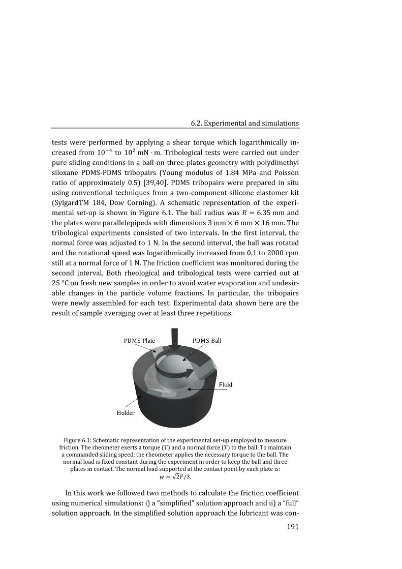
6.2. Experimental and simulations
191
tests were performed by applying a shear torque which logarithmically in-
creased from 10−4 to 102 mN · m. Tribological tests were carried out under
pure sliding conditions in a ball-on-three-plates geometry with polydimethyl
siloxane PDMS-PDMS tribopairs (Young modulus of 1.84 MPa and Poisson
ratio of approximately 0.5) [39,40]. PDMS tribopairs were prepared in situ
using conventional techniques from a two-component silicone elastomer kit
(SylgardTM 184, Dow Corning). A schematic representation of the experi-
mental set-up is shown in Figure 6.1. The ball radius was 𝑅 = 6.35 mm and
the plates were parallelepipeds with dimensions 3 mm × 6 mm × 16 mm. The
tribological experiments consisted of two intervals. In the first interval, the
normal force was adjusted to 1 N. In the second interval, the ball was rotated
and the rotational speed was logarithmically increased from 0.1 to 2000 rpm
still at a normal force of 1 N. The friction coefficient was monitored during the
second interval. Both rheological and tribological tests were carried out at
25 °C on fresh new samples in order to avoid water evaporation and undesir-
able changes in the particle volume fractions. In particular, the tribopairs
were newly assembled for each test. Experimental data shown here are the
result of sample averaging over at least three repetitions.
Figure 6.1: Schematic representation of the experimental set-up employed to measure friction. The rheometer exerts a torque (𝑇) and a normal force (𝑇) to the ball. To maintain a commanded sliding speed, the rheometer applies the necessary torque to the ball. The normal load is fixed constant during the experiment in order to keep the ball and three
plates in contact. The normal load supported at the contact point by each plate is:
𝑤 = √2𝐹/3.
In this work we followed two methods to calculate the friction coefficient
using numerical simulations: i) a “simplified” solution approach and ii) a “full”
solution approach. In the simplified solution approach the lubricant was con-
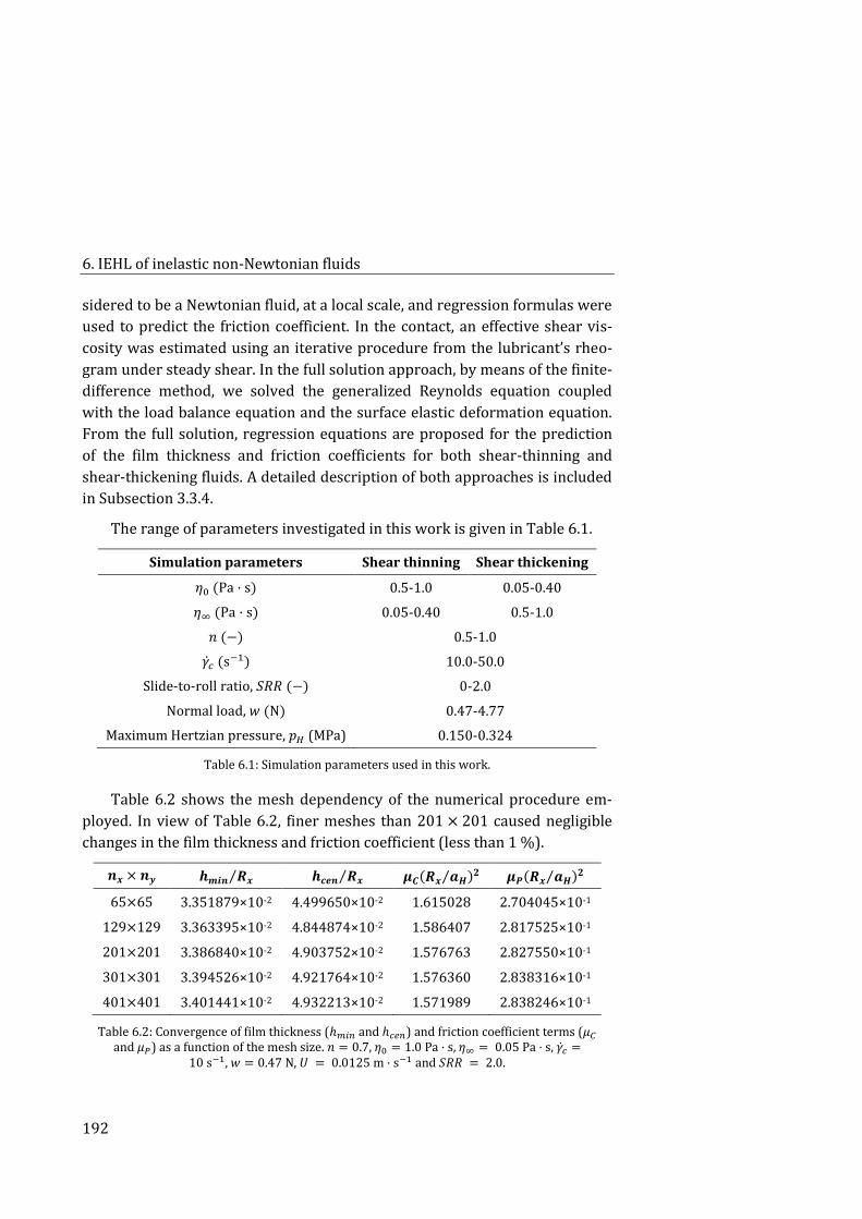
6. IEHL of inelastic non-Newtonian fluids
192
sidered to be a Newtonian fluid, at a local scale, and regression formulas were
used to predict the friction coefficient. In the contact, an effective shear vis-
cosity was estimated using an iterative procedure from the lubricant’s rheo-
gram under steady shear. In the full solution approach, by means of the finite-
difference method, we solved the generalized Reynolds equation coupled
with the load balance equation and the surface elastic deformation equation.
From the full solution, regression equations are proposed for the prediction
of the film thickness and friction coefficients for both shear-thinning and
shear-thickening fluids. A detailed description of both approaches is included
in Subsection 3.3.4.
The range of parameters investigated in this work is given in Table 6.1.
Simulation parameters Shear thinning Shear thickening
휂0 (Pa · s) 0.5-1.0 0.05-0.40
휂∞ (Pa · s) 0.05-0.40 0.5-1.0
𝑛 (−) 0.5-1.0
�̇�𝑐 (s−1) 10.0-50.0
Slide-to-roll ratio, 𝑆𝑅𝑅 (−) 0-2.0
Normal load, 𝑤 (N) 0.47-4.77
Maximum Hertzian pressure, 𝑝𝐻 (MPa) 0.150-0.324
Table 6.1: Simulation parameters used in this work.
Table 6.2 shows the mesh dependency of the numerical procedure em-
ployed. In view of Table 6.2, finer meshes than 201 × 201 caused negligible
changes in the film thickness and friction coefficient (less than 1 %).
𝒏𝒙 × 𝒏𝒚 𝒉𝒎𝒊𝒏 𝑹𝒙⁄ 𝒉𝒄𝒆𝒏 𝑹𝒙⁄ 𝝁𝑪(𝑹𝒙 𝒂𝑯⁄ )𝟐 𝝁𝑷(𝑹𝒙 𝒂𝑯⁄ )𝟐
65×65 3.351879×10⁻² 4.499650×10⁻² 1.615028 2.704045×10⁻¹
129×129 3.363395×10⁻² 4.844874×10⁻² 1.586407 2.817525×10⁻¹
201×201 3.386840×10⁻² 4.903752×10⁻² 1.576763 2.827550×10⁻¹
301×301 3.394526×10⁻² 4.921764×10⁻² 1.576360 2.838316×10⁻¹
401×401 3.401441×10⁻² 4.932213×10⁻² 1.571989 2.838246×10⁻¹
Table 6.2: Convergence of film thickness (ℎ𝑚𝑖𝑛 and ℎ𝑐𝑒𝑛) and friction coefficient terms (𝜇𝐶 and 𝜇𝑃) as a function of the mesh size. 𝑛 = 0.7, 휂0 = 1.0 Pa · s, 휂∞ = 0.05 Pa · s, �̇�𝑐 =
10 s−1, 𝑤 = 0.47 N, 𝑈 = 0.0125 m · s−1 and 𝑆𝑅𝑅 = 2.0.
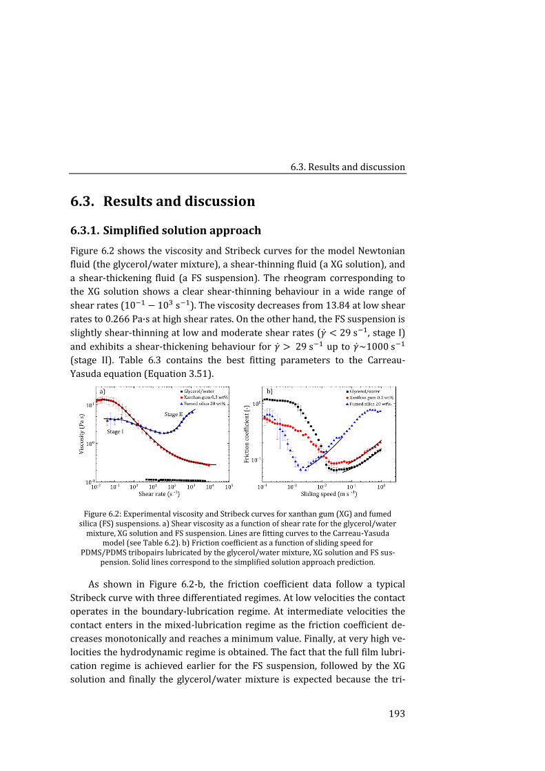
6.3. Results and discussion
193
6.3. Results and discussion
6.3.1. Simplified solution approach
Figure 6.2 shows the viscosity and Stribeck curves for the model Newtonian
fluid (the glycerol/water mixture), a shear-thinning fluid (a XG solution), and
a shear-thickening fluid (a FS suspension). The rheogram corresponding to
the XG solution shows a clear shear-thinning behaviour in a wide range of
shear rates (10−1 − 103 s−1). The viscosity decreases from 13.84 at low shear
rates to 0.266 Pa·s at high shear rates. On the other hand, the FS suspension is
slightly shear-thinning at low and moderate shear rates (�̇� < 29 s−1, stage I)
and exhibits a shear-thickening behaviour for �̇� > 29 s−1 up to �̇�~1000 s−1
(stage II). Table 6.3 contains the best fitting parameters to the Carreau-
Yasuda equation (Equation 3.51).
Figure 6.2: Experimental viscosity and Stribeck curves for xanthan gum (XG) and fumed silica (FS) suspensions. a) Shear viscosity as a function of shear rate for the glycerol/water
mixture, XG solution and FS suspension. Lines are fitting curves to the Carreau-Yasuda model (see Table 6.2). b) Friction coefficient as a function of sliding speed for
PDMS/PDMS tribopairs lubricated by the glycerol/water mixture, XG solution and FS sus-pension. Solid lines correspond to the simplified solution approach prediction.
As shown in Figure 6.2-b, the friction coefficient data follow a typical
Stribeck curve with three differentiated regimes. At low velocities the contact
operates in the boundary-lubrication regime. At intermediate velocities the
contact enters in the mixed-lubrication regime as the friction coefficient de-
creases monotonically and reaches a minimum value. Finally, at very high ve-
locities the hydrodynamic regime is obtained. The fact that the full film lubri-
cation regime is achieved earlier for the FS suspension, followed by the XG
solution and finally the glycerol/water mixture is expected because the tri-
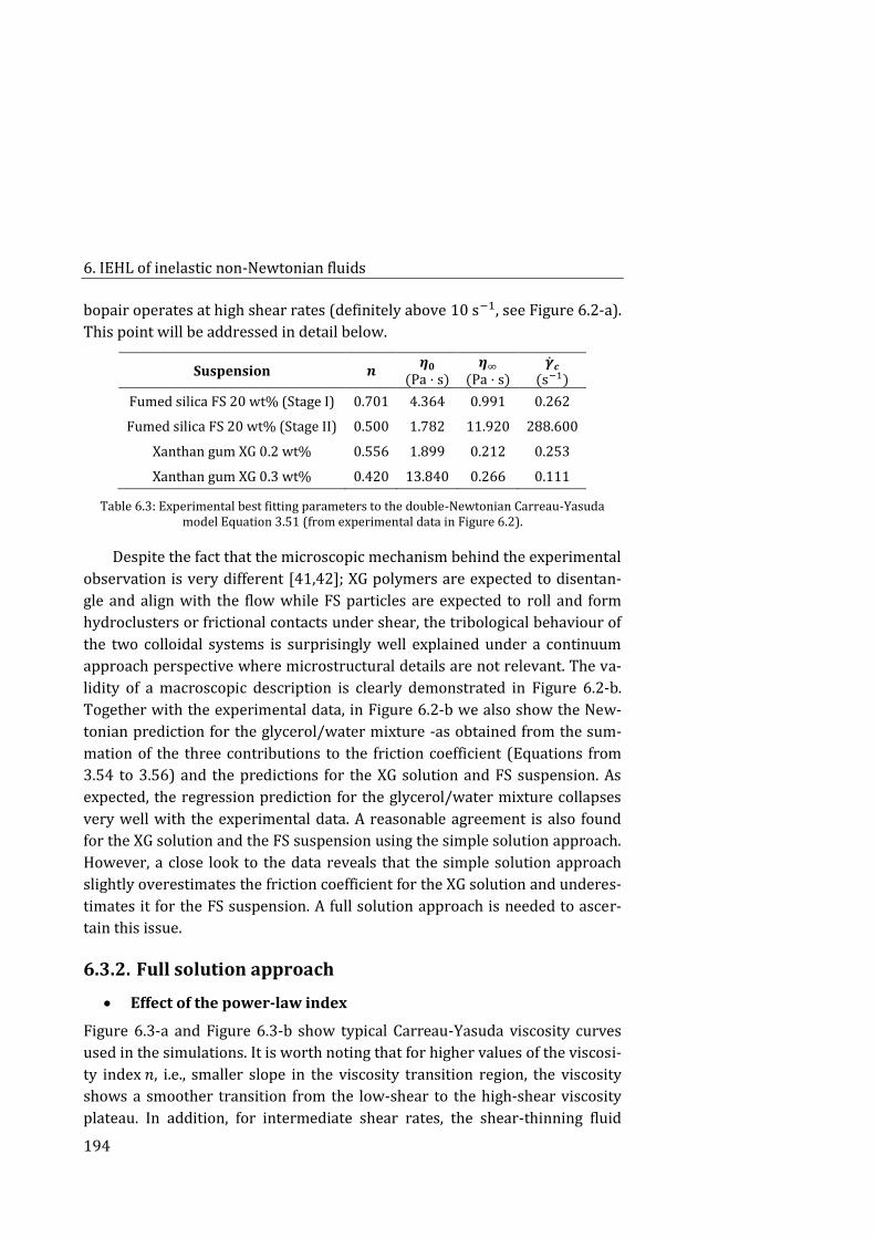
6. IEHL of inelastic non-Newtonian fluids
194
bopair operates at high shear rates (definitely above 10 s−1, see Figure 6.2-a).
This point will be addressed in detail below.
Suspension 𝒏 𝜼𝟎
(Pa · s) 𝜼∞
(Pa · s) �̇�𝒄
(s−1)
Fumed silica FS 20 wt% (Stage I) 0.701 4.364 0.991 0.262
Fumed silica FS 20 wt% (Stage II) 0.500 1.782 11.920 288.600
Xanthan gum XG 0.2 wt% 0.556 1.899 0.212 0.253
Xanthan gum XG 0.3 wt% 0.420 13.840 0.266 0.111
Table 6.3: Experimental best fitting parameters to the double-Newtonian Carreau-Yasuda model Equation 3.51 (from experimental data in Figure 6.2).
Despite the fact that the microscopic mechanism behind the experimental
observation is very different [41,42]; XG polymers are expected to disentan-
gle and align with the flow while FS particles are expected to roll and form
hydroclusters or frictional contacts under shear, the tribological behaviour of
the two colloidal systems is surprisingly well explained under a continuum
approach perspective where microstructural details are not relevant. The va-
lidity of a macroscopic description is clearly demonstrated in Figure 6.2-b.
Together with the experimental data, in Figure 6.2-b we also show the New-
tonian prediction for the glycerol/water mixture -as obtained from the sum-
mation of the three contributions to the friction coefficient (Equations from
3.54 to 3.56) and the predictions for the XG solution and FS suspension. As
expected, the regression prediction for the glycerol/water mixture collapses
very well with the experimental data. A reasonable agreement is also found
for the XG solution and the FS suspension using the simple solution approach.
However, a close look to the data reveals that the simple solution approach
slightly overestimates the friction coefficient for the XG solution and underes-
timates it for the FS suspension. A full solution approach is needed to ascer-
tain this issue.
6.3.2. Full solution approach
Effect of the power-law index
Figure 6.3-a and Figure 6.3-b show typical Carreau-Yasuda viscosity curves
used in the simulations. It is worth noting that for higher values of the viscosi-
ty index 𝑛, i.e., smaller slope in the viscosity transition region, the viscosity
shows a smoother transition from the low-shear to the high-shear viscosity
plateau. In addition, for intermediate shear rates, the shear-thinning fluid
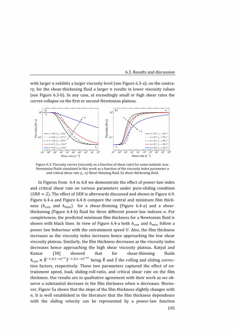
6.3. Results and discussion
195
with larger 𝑛 exhibits a larger viscosity level (see Figure 6.3-a); on the contra-
ry, for the shear-thickening fluid a larger 𝑛 results in lower viscosity values
(see Figure 6.3-b). In any case, at exceedingly small or high shear rates the
curves collapse on the first or second-Newtonian plateau.
Figure 6.3: Viscosity curves (viscosity as a function of shear rate) for some inelastic non-Newtonian fluids simulated in this work as a function of the viscosity index parameter 𝑛
and critical shear rate �̇�𝑐 . a) Shear-thinning fluid, b) shear-thickening fluid.
In Figures from 6.4 to 6.8 we demonstrate the effect of power-law index
and critical shear rate on various parameters under pure-sliding condition
(𝑆𝑅𝑅 = 2). The effect of 𝑆𝑅𝑅 is afterwards discussed and shown in Figure 6.9.
Figure 6.4-a and Figure 6.4-b compare the central and minimum film thick-
ness (ℎ𝑐𝑒𝑛 and ℎ𝑚𝑖𝑛) for a shear-thinning (Figure 6.4-a) and a shear-
thickening (Figure 6.4-b) fluid for three different power-law indexes 𝑛. For
completeness, the predicted minimum film thickness for a Newtonian fluid is
shown with black lines. In view of Figure 6.4-a both ℎ𝑐𝑒𝑛 and ℎ𝑚𝑖𝑛 follow a
power law behaviour with the entrainment speed 𝑈. Also, the film thickness
increases as the viscosity index increases hence approaching the low shear
viscosity plateau. Similarly, the film thickness decreases as the viscosity index
decreases hence approaching the high shear viscosity plateau. Katyal and
Kumar [30] showed that for shear-thinning fluids
ℎ𝑐𝑒𝑛 ∝ �̅�−1.3(1−𝑛)1.3𝑆̅−1.2(1−𝑛)1.92
being �̅� and 𝑆̅ the rolling and sliding correc-
tion factors, respectively. These two parameters captured the effect of en-
trainment speed, load, sliding-roll-ratio, and critical shear rate on the film
thickness. Our results are in qualitative agreement with their work as we ob-
serve a substantial decrease in the film thickness when 𝑛 decreases. Moreo-
ver, Figure 5a shows that the slope of the film thickness slightly changes with
𝑛. It is well established in the literature that the film thickness dependence
with the sliding velocity can be represented by a power-law function
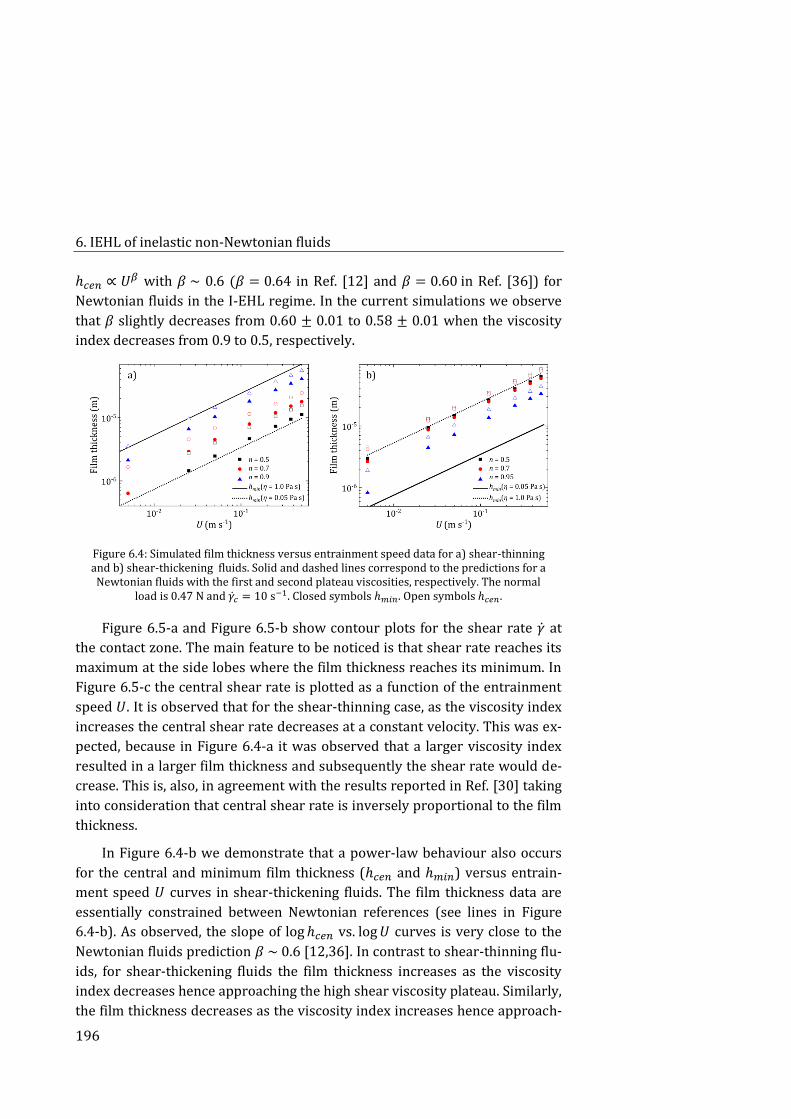
6. IEHL of inelastic non-Newtonian fluids
196
ℎ𝑐𝑒𝑛 ∝ 𝑈𝛽 with 𝛽 ~ 0.6 (𝛽 = 0.64 in Ref. [12] and 𝛽 = 0.60 in Ref. [36]) for
Newtonian fluids in the I-EHL regime. In the current simulations we observe
that 𝛽 slightly decreases from 0.60 ± 0.01 to 0.58 ± 0.01 when the viscosity
index decreases from 0.9 to 0.5, respectively.
Figure 6.4: Simulated film thickness versus entrainment speed data for a) shear-thinning and b) shear-thickening fluids. Solid and dashed lines correspond to the predictions for a Newtonian fluids with the first and second plateau viscosities, respectively. The normal
load is 0.47 N and �̇�𝑐 = 10 s−1. Closed symbols ℎ𝑚𝑖𝑛. Open symbols ℎ𝑐𝑒𝑛.
Figure 6.5-a and Figure 6.5-b show contour plots for the shear rate �̇� at
the contact zone. The main feature to be noticed is that shear rate reaches its
maximum at the side lobes where the film thickness reaches its minimum. In
Figure 6.5-c the central shear rate is plotted as a function of the entrainment
speed 𝑈. It is observed that for the shear-thinning case, as the viscosity index
increases the central shear rate decreases at a constant velocity. This was ex-
pected, because in Figure 6.4-a it was observed that a larger viscosity index
resulted in a larger film thickness and subsequently the shear rate would de-
crease. This is, also, in agreement with the results reported in Ref. [30] taking
into consideration that central shear rate is inversely proportional to the film
thickness.
In Figure 6.4-b we demonstrate that a power-law behaviour also occurs
for the central and minimum film thickness (ℎ𝑐𝑒𝑛 and ℎ𝑚𝑖𝑛) versus entrain-
ment speed 𝑈 curves in shear-thickening fluids. The film thickness data are
essentially constrained between Newtonian references (see lines in Figure
6.4-b). As observed, the slope of log ℎ𝑐𝑒𝑛 vs. log 𝑈 curves is very close to the
Newtonian fluids prediction 𝛽 ~ 0.6 [12,36]. In contrast to shear-thinning flu-
ids, for shear-thickening fluids the film thickness increases as the viscosity
index decreases hence approaching the high shear viscosity plateau. Similarly,
the film thickness decreases as the viscosity index increases hence approach-
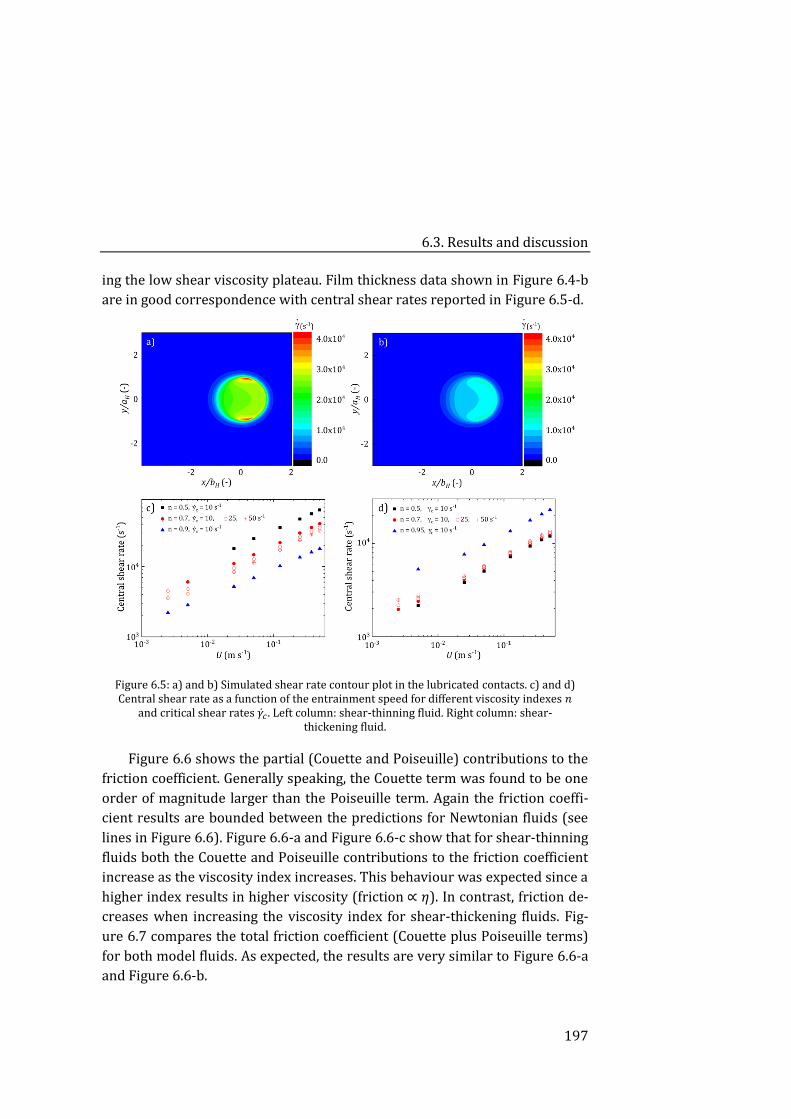
6.3. Results and discussion
197
ing the low shear viscosity plateau. Film thickness data shown in Figure 6.4-b
are in good correspondence with central shear rates reported in Figure 6.5-d.
Figure 6.5: a) and b) Simulated shear rate contour plot in the lubricated contacts. c) and d) Central shear rate as a function of the entrainment speed for different viscosity indexes 𝑛
and critical shear rates �̇�𝑐 . Left column: shear-thinning fluid. Right column: shear-thickening fluid.
Figure 6.6 shows the partial (Couette and Poiseuille) contributions to the
friction coefficient. Generally speaking, the Couette term was found to be one
order of magnitude larger than the Poiseuille term. Again the friction coeffi-
cient results are bounded between the predictions for Newtonian fluids (see
lines in Figure 6.6). Figure 6.6-a and Figure 6.6-c show that for shear-thinning
fluids both the Couette and Poiseuille contributions to the friction coefficient
increase as the viscosity index increases. This behaviour was expected since a
higher index results in higher viscosity (friction ∝ 휂). In contrast, friction de-
creases when increasing the viscosity index for shear-thickening fluids. Fig-
ure 6.7 compares the total friction coefficient (Couette plus Poiseuille terms)
for both model fluids. As expected, the results are very similar to Figure 6.6-a
and Figure 6.6-b.
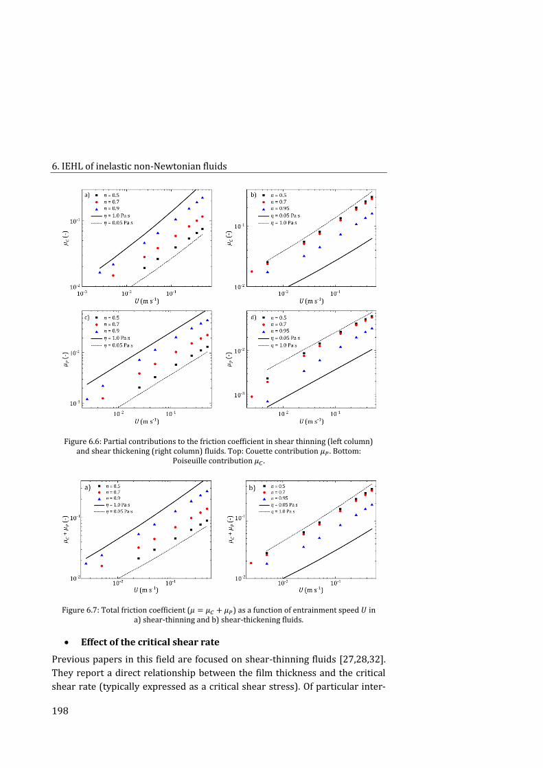
6. IEHL of inelastic non-Newtonian fluids
198
Figure 6.6: Partial contributions to the friction coefficient in shear thinning (left column) and shear thickening (right column) fluids. Top: Couette contribution 𝜇𝑃 . Bottom:
Poiseuille contribution 𝜇𝐶 .
Figure 6.7: Total friction coefficient (𝜇 = 𝜇𝐶 + 𝜇𝑃) as a function of entrainment speed 𝑈 in a) shear-thinning and b) shear-thickening fluids.
Effect of the critical shear rate
Previous papers in this field are focused on shear-thinning fluids [27,28,32].
They report a direct relationship between the film thickness and the critical
shear rate (typically expressed as a critical shear stress). Of particular inter-
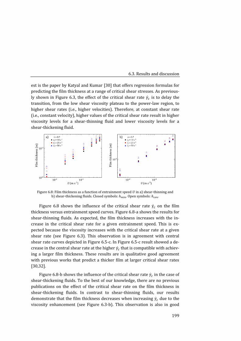
6.3. Results and discussion
199
est is the paper by Katyal and Kumar [30] that offers regression formulas for
predicting the film thickness at a range of critical shear stresses. As previous-
ly shown in Figure 6.3, the effect of the critical shear rate �̇�𝑐 is to delay the
transition, from the low shear viscosity plateau to the power-law region, to
higher shear rates (i.e., higher velocities). Therefore, at constant shear rate
(i.e., constant velocity), higher values of the critical shear rate result in higher
viscosity levels for a shear-thinning fluid and lower viscosity levels for a
shear-thickening fluid.
Figure 6.8: Film thickness as a function of entrainment speed 𝑈 in a) shear-thinning and b) shear-thickening fluids. Closed symbols: ℎ𝑚𝑖𝑛. Open symbols: ℎ𝑐𝑒𝑛.
Figure 6.8 shows the influence of the critical shear rate �̇�𝑐 on the film
thickness versus entrainment speed curves. Figure 6.8-a shows the results for
shear-thinning fluids. As expected, the film thickness increases with the in-
crease in the critical shear rate for a given entrainment speed. This is ex-
pected because the viscosity increases with the critical shear rate at a given
shear rate (see Figure 6.3). This observation is in agreement with central
shear rate curves depicted in Figure 6.5-c. In Figure 6.5-c result showed a de-
crease in the central shear rate at the higher �̇�𝑐 that is compatible with achiev-
ing a larger film thickness. These results are in qualitative good agreement
with previous works that predict a thicker film at larger critical shear rates
[30,32].
Figure 6.8-b shows the influence of the critical shear rate �̇�𝑐 in the case of
shear-thickening fluids. To the best of our knowledge, there are no previous
publications on the effect of the critical shear rate on the film thickness in
shear-thickening fluids. In contrast to shear-thinning fluids, our results
demonstrate that the film thickness decreases when increasing �̇�𝑐 due to the
viscosity enhancement (see Figure 6.3-b). This observation is also in good
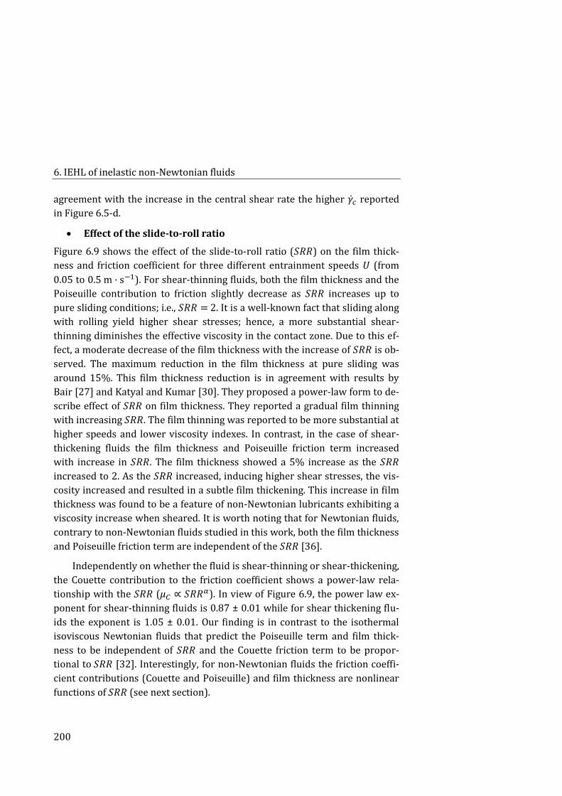
6. IEHL of inelastic non-Newtonian fluids
200
agreement with the increase in the central shear rate the higher �̇�𝑐 reported
in Figure 6.5-d.
Effect of the slide-to-roll ratio
Figure 6.9 shows the effect of the slide-to-roll ratio (𝑆𝑅𝑅) on the film thick-
ness and friction coefficient for three different entrainment speeds 𝑈 (from
0.05 to 0.5 m · s−1). For shear-thinning fluids, both the film thickness and the
Poiseuille contribution to friction slightly decrease as 𝑆𝑅𝑅 increases up to
pure sliding conditions; i.e., 𝑆𝑅𝑅 = 2. It is a well-known fact that sliding along
with rolling yield higher shear stresses; hence, a more substantial shear-
thinning diminishes the effective viscosity in the contact zone. Due to this ef-
fect, a moderate decrease of the film thickness with the increase of 𝑆𝑅𝑅 is ob-
served. The maximum reduction in the film thickness at pure sliding was
around 15%. This film thickness reduction is in agreement with results by
Bair [27] and Katyal and Kumar [30]. They proposed a power-law form to de-
scribe effect of 𝑆𝑅𝑅 on film thickness. They reported a gradual film thinning
with increasing 𝑆𝑅𝑅. The film thinning was reported to be more substantial at
higher speeds and lower viscosity indexes. In contrast, in the case of shear-
thickening fluids the film thickness and Poiseuille friction term increased
with increase in 𝑆𝑅𝑅. The film thickness showed a 5% increase as the 𝑆𝑅𝑅
increased to 2. As the 𝑆𝑅𝑅 increased, inducing higher shear stresses, the vis-
cosity increased and resulted in a subtle film thickening. This increase in film
thickness was found to be a feature of non-Newtonian lubricants exhibiting a
viscosity increase when sheared. It is worth noting that for Newtonian fluids,
contrary to non-Newtonian fluids studied in this work, both the film thickness
and Poiseuille friction term are independent of the 𝑆𝑅𝑅 [36].
Independently on whether the fluid is shear-thinning or shear-thickening,
the Couette contribution to the friction coefficient shows a power-law rela-
tionship with the 𝑆𝑅𝑅 (𝜇𝐶 ∝ 𝑆𝑅𝑅𝛼). In view of Figure 6.9, the power law ex-
ponent for shear-thinning fluids is 0.87 ± 0.01 while for shear thickening flu-
ids the exponent is 1.05 ± 0.01. Our finding is in contrast to the isothermal
isoviscous Newtonian fluids that predict the Poiseuille term and film thick-
ness to be independent of 𝑆𝑅𝑅 and the Couette friction term to be propor-
tional to 𝑆𝑅𝑅 [32]. Interestingly, for non-Newtonian fluids the friction coeffi-
cient contributions (Couette and Poiseuille) and film thickness are nonlinear
functions of 𝑆𝑅𝑅 (see next section).
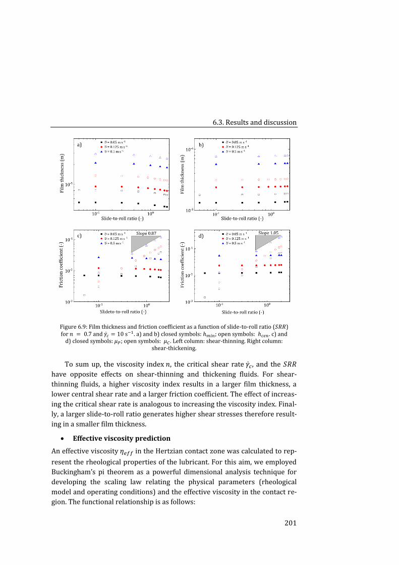
6.3. Results and discussion
201
Figure 6.9: Film thickness and friction coefficient as a function of slide-to-roll ratio (𝑆𝑅𝑅) for 𝑛 = 0.7 and �̇�𝑐 = 10 s−1. a) and b) closed symbols: ℎ𝑚𝑖𝑛; open symbols: ℎ𝑐𝑒𝑛. c) and
d) closed symbols: 𝜇𝑃; open symbols: 𝜇𝐶 . Left column: shear-thinning. Right column: shear-thickening.
To sum up, the viscosity index 𝑛, the critical shear rate �̇�𝑐, and the 𝑆𝑅𝑅
have opposite effects on shear-thinning and thickening fluids. For shear-
thinning fluids, a higher viscosity index results in a larger film thickness, a
lower central shear rate and a larger friction coefficient. The effect of increas-
ing the critical shear rate is analogous to increasing the viscosity index. Final-
ly, a larger slide-to-roll ratio generates higher shear stresses therefore result-
ing in a smaller film thickness.
Effective viscosity prediction
An effective viscosity 휂𝑒𝑓𝑓 in the Hertzian contact zone was calculated to rep-
resent the rheological properties of the lubricant. For this aim, we employed
Buckingham’s pi theorem as a powerful dimensional analysis technique for
developing the scaling law relating the physical parameters (rheological
model and operating conditions) and the effective viscosity in the contact re-
gion. The functional relationship is as follows:
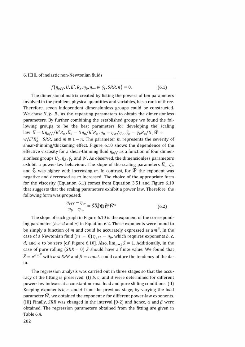
6. IEHL of inelastic non-Newtonian fluids
202
𝑓(휂𝑒𝑓𝑓, 𝑈, 𝐸′, 𝑅𝑥 , 휂0, 휂∞, 𝑤, �̇�𝑐 , 𝑆𝑅𝑅, 𝑛) = 0. (6.1)
The dimensional matrix created by listing the powers of ten parameters
involved in the problem, physical quantities and variables, has a rank of three.
Therefore, seven independent dimensionless groups could be constructed.
We chose 𝑈, �̇�𝑐, 𝑅𝑥 as the repeating parameters to obtain the dimensionless
parameters. By further combining the established groups we found the fol-
lowing groups to be the best parameters for developing the scaling
law: �̅� = 𝑈휂𝑒𝑓𝑓 𝐸′𝑅𝑥⁄ , �̅�0 = 𝑈휂0 𝐸′𝑅𝑥⁄ , 휂̅𝑅 = 휂∞ 휂0⁄ , �̅̇�𝑐 = �̇�𝑐𝑅𝑥 𝑈⁄ , �̅� =
𝑤/𝐸′𝑅𝑥2 , 𝑆𝑅𝑅, and 𝑚 ≡ 1 − 𝑛. The parameter 𝑚 represents the severity of
shear-thinning/thickening effect. Figure 6.10 shows the dependence of the
effective viscosity for a shear-thinning fluid 휂𝑒𝑓𝑓 as a function of four dimen-
sionless groups �̅�0, 휂̅𝑅 , �̅̇�𝑐 and �̅�. As observed, the dimensionless parameters
exhibit a power-law behaviour. The slope of the scaling parameters �̅�0, 휂̅𝑅
and �̅̇�𝑐 was higher with increasing 𝑚. In contrast, for �̅� the exponent was
negative and decreased as 𝑚 increased. The choice of the appropriate form
for the viscosity (Equation 6.1) comes from Equation 3.51 and Figure 6.10
that suggests that the scaling parameters exhibit a power law. Therefore, the
following form was proposed:
휂𝑒𝑓𝑓 − 휂∞
휂0 − 휂∞= 𝑆̅�̅�0
𝑏휂̅𝑅𝑐 �̅̇�𝑐
𝑑�̅�𝑒 (6.2)
The slope of each graph in Figure 6.10 is the exponent of the correspond-
ing parameter (𝑏, 𝑐, 𝑑 and 𝑒) in Equation 6.2. These exponents were found to
be simply a function of 𝑚 and could be accurately expressed as 𝛼𝑚𝛽. In the
case of a Newtonian fluid (𝑚 = 0) 휂𝑒𝑓𝑓 = 휂0, which requires exponents 𝑏, 𝑐,
𝑑, and 𝑒 to be zero [c.f. Figure 6.10]. Also, lim𝑛→1 𝑆̅ = 1. Additionally, in the
case of pure rolling (𝑆𝑅𝑅 = 0) 𝑆̅ should have a finite value. We found that
𝑆̅ = 𝑒𝛼𝑚𝛽 with 𝛼 ∝ 𝑆𝑅𝑅 and 𝛽 = 𝑐𝑜𝑛𝑠𝑡. could capture the tendency of the da-
ta.
The regression analysis was carried out in three stages so that the accu-
racy of the fitting is preserved: (I) 𝑏, 𝑐, and 𝑑 were determined for different
power-law indexes at a constant normal load and pure sliding conditions. (II)
Keeping exponents 𝑏, 𝑐, and 𝑑 from the previous stage, by varying the load
parameter �̅�, we obtained the exponent 𝑒 for different power-law exponents.
(III) Finally, 𝑆𝑅𝑅 was changed in the interval [0-2] and hence, 𝛼 and 𝛽 were
obtained. The regression parameters obtained from the fitting are given in
Table 6.4.
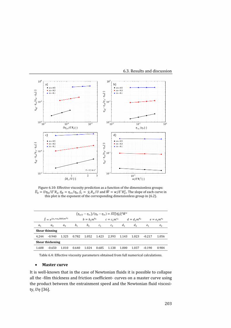
6.3. Results and discussion
203
Figure 6.10: Effective viscosity prediction as a function of the dimensionless groups: �̅�0 = 𝑈휂0 𝐸′𝑅𝑥⁄ , 휂̅𝑅 = 휂∞ 휂0⁄ , �̅̇�𝑐 = �̇�𝑐𝑅𝑥 𝑈⁄ and �̅� = 𝑤/𝐸′𝑅𝑥
2,. The slope of each curve in this plot is the exponent of the corresponding dimensionless group in (6.2).
(휂𝑒𝑓𝑓 − 휂∞) (휂0 − 휂∞)⁄ = 𝑆̅�̅�0𝑏휂̅𝑅
𝑐 �̅̇�𝑐𝑑�̅�𝑒
𝑆̅ = 𝑒 (𝑎1+𝑎2𝑆𝑅𝑅)𝑚𝑎3 𝑏 = 𝑏1𝑚𝑏2 𝑐 = 𝑐1𝑚𝑐2 𝑑 = 𝑑1𝑚𝑑2 𝑒 = 𝑒1𝑚𝑒2
𝑎1 𝑎2 𝑎3 𝑏1 𝑏2 𝑐1 𝑐2 𝑑1 𝑑2 𝑒1 𝑒2
Shear thinning
4.244 -0.940 1.325 0.782 1.052 1.423 2.393 1.143 1.023 -0.217 1.056
Shear thickening
1.608 -0.650 1.010 0.640 1.024 0.685 1.138 1.000 1.037 -0.190 0.984
Table 6.4: Effective viscosity parameters obtained from full numerical calculations.
Master curve
It is well-known that in the case of Newtonian fluids it is possible to collapse
all the -film thickness and friction coefficient- curves on a master curve using
the product between the entrainment speed and the Newtonian fluid viscosi-
ty, 𝑈휂 [36].
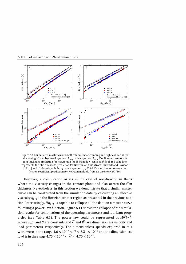
6. IEHL of inelastic non-Newtonian fluids
204
Figure 6.11: Simulated master curves. Left column shear-thinning and right column shear thickening. a) and b) closed symbols: ℎ𝑚𝑖𝑛; open symbols: ℎ𝑐𝑒𝑛 . Dot line represents the film thickness prediction for Newtonian fluids from de Vicente et al. [36] and solid line
represents the film thickness prediction for Newtonian fluids from Hamrock and Dowson [12]. c) and d) closed symbols: 𝜇𝑃; open symbols: 𝜇𝐶/𝑆𝑅𝑅. Dashed line represents the
friction coefficient prediction for Newtonian fluids from de Vicente et al. [36].
However, a complication arises in the case of non-Newtonian fluids
where the viscosity changes in the contact plane and also across the film
thickness. Nevertheless, in this section we demonstrate that a similar master
curve can be constructed from the simulation data by calculating an effective
viscosity 휂𝑒𝑓𝑓 in the Hertzian contact region as presented in the previous sec-
tion. Interestingly, 𝑈휂𝑒𝑓𝑓 is capable to collapse all the data on a master curve
following a power-law function. Figure 6.11 shows the collapse of the simula-
tion results for combinations of the operating parameters and lubricant prop-
erties (see Table 6.1). The power law could be represented as 𝛼�̅�𝛽�̅�𝜃,
where 𝛼, 𝛽, and 휃 are constants and �̅� and �̅� are dimensionless velocity and
load parameters, respectively. The dimensionless speeds explored in this
work were in the range 1.6 × 10⁻⁷ < �̅� < 3.21 × 10⁻⁵ and the dimensionless
load is in the range 4.75 × 10⁻³ < �̅� < 4.75 × 10⁻².
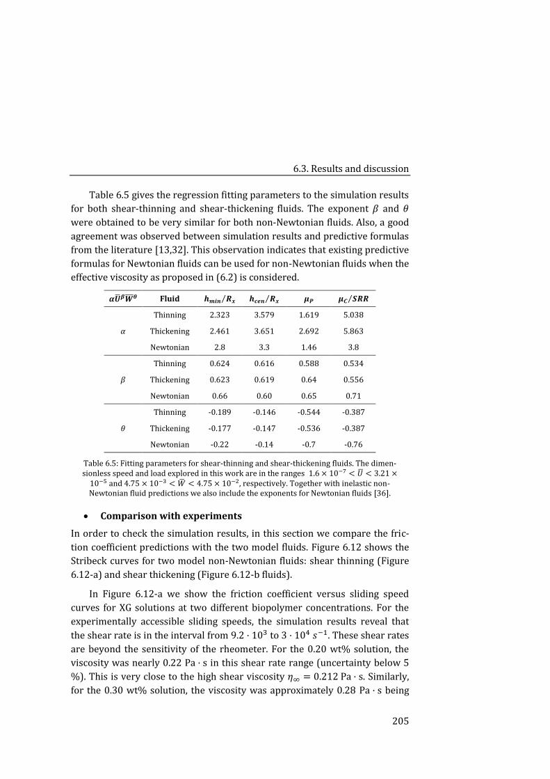
6.3. Results and discussion
205
Table 6.5 gives the regression fitting parameters to the simulation results
for both shear-thinning and shear-thickening fluids. The exponent 𝛽 and 휃
were obtained to be very similar for both non-Newtonian fluids. Also, a good
agreement was observed between simulation results and predictive formulas
from the literature [13,32]. This observation indicates that existing predictive
formulas for Newtonian fluids can be used for non-Newtonian fluids when the
effective viscosity as proposed in (6.2) is considered.
𝜶�̅�𝜷�̅̅̅�𝜽 Fluid 𝒉𝒎𝒊𝒏 𝑹𝒙⁄ 𝒉𝒄𝒆𝒏 𝑹𝒙⁄ 𝝁𝑷 𝝁𝑪 𝑺𝑹𝑹⁄
𝛼
Thinning 2.323 3.579 1.619 5.038
Thickening 2.461 3.651 2.692 5.863
Newtonian 2.8 3.3 1.46 3.8
𝛽
Thinning 0.624 0.616 0.588 0.534
Thickening 0.623 0.619 0.64 0.556
Newtonian 0.66 0.60 0.65 0.71
휃
Thinning -0.189 -0.146 -0.544 -0.387
Thickening -0.177 -0.147 -0.536 -0.387
Newtonian -0.22 -0.14 -0.7 -0.76
Table 6.5: Fitting parameters for shear-thinning and shear-thickening fluids. The dimen-sionless speed and load explored in this work are in the ranges 1.6 × 10⁻⁷ < �̅� < 3.21 ×
10−5 and 4.75 × 10⁻³ < �̅� < 4.75 × 10⁻², respectively. Together with inelastic non-Newtonian fluid predictions we also include the exponents for Newtonian fluids [36].
Comparison with experiments
In order to check the simulation results, in this section we compare the fric-
tion coefficient predictions with the two model fluids. Figure 6.12 shows the
Stribeck curves for two model non-Newtonian fluids: shear thinning (Figure
6.12-a) and shear thickening (Figure 6.12-b fluids).
In Figure 6.12-a we show the friction coefficient versus sliding speed
curves for XG solutions at two different biopolymer concentrations. For the
experimentally accessible sliding speeds, the simulation results reveal that
the shear rate is in the interval from 9.2 · 103 to 3 · 104 𝑠−1. These shear rates
are beyond the sensitivity of the rheometer. For the 0.20 wt% solution, the
viscosity was nearly 0.22 Pa · s in this shear rate range (uncertainty below 5
%). This is very close to the high shear viscosity 휂∞ = 0.212 Pa · s. Similarly,
for the 0.30 wt% solution, the viscosity was approximately 0.28 Pa · s being
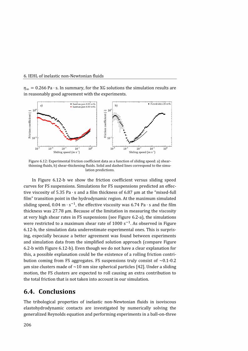
6. IEHL of inelastic non-Newtonian fluids
206
휂∞ = 0.266 Pa · s. In summary, for the XG solutions the simulation results are
in reasonably good agreement with the experiments.
Figure 6.12: Experimental friction coefficient data as a function of sliding speed: a) shear-thinning fluids, b) shear-thickening fluids. Solid and dashed lines correspond to the simu-
lation predictions.
In Figure 6.12-b we show the friction coefficient versus sliding speed
curves for FS suspensions. Simulations for FS suspensions predicted an effec-
tive viscosity of 5.35 Pa · s and a film thickness of 6.87 μm at the “mixed-full
film” transition point in the hydrodynamic region. At the maximum simulated
sliding speed, 0.04 m · s−1, the effective viscosity was 6.74 Pa · s and the film
thickness was 27.78 μm. Because of the limitation in measuring the viscosity
at very high shear rates in FS suspensions (see Figure 6.2-a), the simulations
were restricted to a maximum shear rate of 1000 s−1. As observed in Figure
6.12-b, the simulation data underestimate experimental ones. This is surpris-
ing, especially because a better agreement was found between experiments
and simulation data from the simplified solution approach (compare Figure
6.2-b with Figure 6.12-b). Even though we do not have a clear explanation for
this, a possible explanation could be the existence of a rolling friction contri-
bution coming from FS aggregates. FS suspensions truly consist of ~0.1-0.2
μm size clusters made of ~10 nm size spherical particles [42]. Under a sliding
motion, the FS clusters are expected to roll causing an extra contribution to
the total friction that is not taken into account in our simulation.
6.4. Conclusions
The tribological properties of inelastic non-Newtonian fluids in isoviscous
elastohydrodynamic contacts are investigated by numerically solving the
generalized Reynolds equation and performing experiments in a ball-on-three
6.4. Conclusions
207
plates tribometer. Two particular lubricants are investigated: shear-thinning
and shear-thickening fluids.
A double-Newtonian Carreau-Yasuda model is used to describe the vis-
cosity thinning and thickening under increasing shear rates. First, a simplified
solution approach is proposed to estimate the film thickness and the friction
coefficient. In this approach, the fluid viscosity is estimated, using an iterative
procedure, from the experimental viscosity curve as a function of the shear
rate. Second, a full solution approach is described where the generalized
Reynolds equation is numerically solved. Regression formulas are presented
to define an effective lubricant viscosity. Interestingly, this effective viscosity
is capable to collapse all the simulation data on a master curve where the fric-
tion coefficient is plotted as function of the entrainment speed multiplied by
the effective viscosity. Regression formulas are also proposed for the film
thickness.
A reasonably good agreement is obtained when comparing the simulation
predictions and experimental data on model inelastic non-Newtonian fluids:
xanthan gum solutions and fumed silica suspensions.
6.5. References
[1] Timm K, Myant C, Spikes H A and Grunze M 2011 Particulate lubri-cants in cosmetic applications Tribol. Int. 44 1695–1703
[2] Yakubov G E, Branfield T E, Bongaerts J H H and Stokes J R 2015 Tri-bology of particle suspensions in rolling-sliding soft contacts Biotribology 3 1–10
[3] Zhang B, Selway N, Shelat K J, Dhital S, Stokes J R and Gidley M J 2017 Tribology of swollen starch granule suspensions from maize and potato Car-bohydr. Polym. 155 128–135
[4] Olivares M L, Shahrivar K and Vicente J de 2019 Soft lubrication char-acteristics of microparticulated whey proteins used as fat replacers in dairy systems J. Food Eng. 245 157–165
[5] Esfahanian M and Hamrock B J 1991 Fluid-film lubrication regimes revisited Tribol. Trans. 34 628–632
[6] Pradal C and Stokes J R 2016 Oral tribology: bridging the gap between physical measurements and sensory experience Curr. Opin. Food Sci. 9 34–41
[7] Jin Z and Dowson D 2005 Elastohydrodynamic lubrication in biologi-cal systems Proc. Inst. Mech. Eng. Part J J. Eng. Tribol. 219 367–380
6. IEHL of inelastic non-Newtonian fluids
208
[8] Reynolds O 1886 On the theory of lubrication and its application to Mr. Beauchamp Tower’s experiments, including an experimental determina-tion of the viscosity of olive oil Philos. Trans. R. Soc. Lond. 177 157–234
[9] Grubin A N 1949 Investigation of the contact of machine components Cent. Sci. Res. Inst Tech Mech Eng
[10] Dowson D and Higginson G R 1959 A numerical solution to the elasto-hydrodynamic problem J. Mech. Eng. Sci. 1 6–15
[11] Dowson D 1966 Elastohydrodynamic lubrication Fundam. Roll. Gear Lubr.
[12] Hamrock B J and Dowson D 1976 Isothermal elastohydrodynamic lu-brication of point contacts: Part 1—Theoretical formulation J. Lubr. Technol. 98 223
[13] Hamrock B, Schmid S and Jacobson B 2004 Fundamentals of Fluid Film Lubrication (CRC Press)
[14] Lugt P M and Morales-Espejel G E 2011 A Review of Elasto-Hydrodynamic Lubrication Theory Tribol. Trans. 54 470–496
[15] Lubrecht A A, Napel W E ten and Bosma R 1987 Multigrid, an alterna-tive method of solution for two-dimensional elastohydrodynamically lubri-cated point contact calculations J. Tribol. 109 437
[16] Nijenbanning G, Venner C H and Moes H 1994 Film thickness in elas-tohydrodynamically lubricated elliptic contacts Wear 176 217–229
[17] Venner C H and Lubrecht A A 2000 Multilevel methods in lubrication (Amsterdam ; New York: Elsevier)
[18] Hooke C J 2000 The behaviour of low-amplitude surface roughness under line contacts: Non-Newtonian fluids Proc. Inst. Mech. Eng. Part J J. Eng. Tribol. 214 253–265
[19] Ehret P, Dowson D and Taylor C M 1998 On lubricant transport condi-tions in elastohydrodynamic conjuctions Proc. R. Soc. Lond. Ser. Math. Phys. Eng. Sci. 454 763–787
[20] Greenwood J A and Kauzlarich J J 1998 Elastohydrodynamic film thickness for shear-thinning lubricants Proc. Inst. Mech. Eng. Part J J. Eng. Tri-bol. 212 179–191
[21] Greenwood J A 2000 Two-dimensional flow of a non-Newtonian lubri-cant Proc. Inst. Mech. Eng. Part J J. Eng. Tribol. 214 29–41
[22] Liu Y, Wang Q J, Bair S and Vergne P 2007 A quantitative solution for the full shear-thinning EHL point contact problem including traction Tribol. Lett. 28 171–181
6.5. References
209
[23] Jang J Y, Khonsari M M and Bair S 2007 On the elastohydrodynamic analysis of shear-thinning fluids Proc. R. Soc. Math. Phys. Eng. Sci. 463 3271–3290
[24] Bair S and Qureshi F 2003 The generalized Newtonian fluid model and elastohydrodynamic film thickness J. Tribol. 125 70
[25] de la Guerra Ochoa E, Echávarri Otero J, Chacón Tanarro E and del Río López B 2018 A thermal resistances-based approach for thermal-elastohydrodynamic calculations in point contacts Proc. Inst. Mech. Eng. Part C J. Mech. Eng. Sci. 232 2088–102
[26] de la Guerra Ochoa E, Echávarri Otero J, Sánchez López A, Chacón Tanarro E and del Río López B 2018 Film thickness formula for thermal EHL line contact considering a new Reynolds–Carreau equation Tribol. Lett. 66
[27] Bair S 2005 Shear thinning correction for rolling/sliding elastohydro-dynamic film thickness Proc. Inst. Mech. Eng. Part J J. Eng. Tribol. 219 69–74
[28] Kumar P and Khonsari M M 2008 EHL circular contact film thickness correction factor for shear-thinning fluids J. Tribol. 130 041506
[29] Katyal P and Kumar P 2012 Central film thickness formula for shear thinning lubricants in EHL point contacts under pure rolling Tribol. Int. 48 113–121
[30] Katyal P and Kumar P 2014 New central film thickness equation for shear thinning lubricants in elastohydrodynamic lubricated rolling/sliding point contact conditions J. Tribol. 136 041504
[31] Habchi W, Vergne P, Eyheramendy D and Morales-Espejel G E 2011 Numerical investigation of the use of machinery low-viscosity working fluids as lubricants in elastohydrodynamic lubricated point contacts Proc. Inst. Mech. Eng. Part J J. Eng. Tribol. 225 465–477
[32] Jang J Y, Khonsari M M and Bair S 2008 Correction factor formula to predict the central and minimum film thickness for shear-thinning fluids in EHL J. Tribol. 130 024501
[33] Habchi W, Bair S, Qureshi F and Covitch M 2013 A film thickness cor-rection formula for double-Newtonian shear-thinning in rolling EHL circular contacts Tribol. Lett. 50 59–66
[34] Katyal P and Kumar P 2014 On the role of second Newtonian viscosity in EHL point contacts using double Newtonian shear-thinning model Tribol. Int. 71 140–148
[35] Bair S 2018 Generalized Newtonian viscosity functions for hydrody-namic lubrication Tribol. Int. 117 15–23
6. IEHL of inelastic non-Newtonian fluids
210
[36] de Vicente J, Stokes J R and Spikes H A 2005 The frictional properties of Newtonian fluids in rolling–sliding soft-EHL contact Tribol. Lett. 20 273–86
[37] de Vicente J, Stokes J R and Spikes H A 2006 Soft lubrication of model hydrocolloids Food Hydrocoll. 20 483–91
[38] Raghavan S R and Khan S A 1997 Shear-thickening response of fumed silica suspensions under steady and oscillatory shear J. Colloid Interface Sci. 185 57–67
[39] Shahrivar K and de Vicente J 2014 Ferrofluid lubrication of compliant polymeric contacts: effect of non-homogeneous magnetic fields Tribol. Lett. 56 281–92
[40] Bombard A J F and de Vicente J 2012 Boundary lubrication of magne-torheological fluids in PTFE/steel point contacts Wear 296 484–90
[41] de Vicente J, Stokes J R and Spikes H A 2005 Lubrication properties of non-adsorbing polymer solutions in soft elastohydrodynamic (EHD) contacts Tribol. Int. 38 515–26
[42] Raghavan S R, Walls H J and Khan S A 2000 Rheology of silica disper-sions in organic liquids: new evidence for solvation forces dictated by hydro-gen bonding Langmuir 16 7920–7930
211
7. Soft lubrication of cornstarch-based
shear-thickening fluids
E.M. Ortigosa-Moya, K. Shahrivar, R. Hidalgo-Álvarez, J. de Vicente
The content of this chapter is published in: Smart Materials and Struc-
tures, 2019, 28, 085044 (12 pp).
https://doi.org/10.1088/1361-665X/ab22e5
Abstract
The behaviour of complex fluids in thin films under the isoviscous elastohy-
drodynamic lubrication regime is a topic of current interest. A vast majority
of the materials used to lubricate compliant contacts are shear-thinning fluids
and, in comparison, very little is known about the lubrication properties of
shear-thickening (ST) fluids. In this work we carried out both rheological and
tribological experiments on ST fluids based on cornstarch suspensions. We
investigated the influence of the polarity and viscosity of the carrier fluid and
the cornstarch particles’ concentration. From a rheological perspective, the
ST response is diminished (as the shear-thinning region enlarges) when non-
polar carriers are used (e.g., silicone oil) while a marked thickening is ob-
served for polar carriers (e.g., glycerol-water mixtures). From a tribological
perspective, the friction coefficient at slow sliding speeds is strongly affected
7. Soft lubrication of cornstarch-based shear-thickening fluids
212
by the nature of the carrier fluid, and in particular its wettability in contact
with hydrophobic PDMS tribopairs. We demonstrate that experimental data,
plotted in terms of Stribeck curves, provide useful information on the en-
trainment of particles/fluid through the contact. Finally, experimental results
are also compared with numerical solutions of the Reynolds equation for ine-
lastic non-Newtonian fluids in the isoviscous elastohydrodynamic regime. A
Carreau–Yasuda constitutive equation for the viscosity-shear rate relation-
ship is used.
7.1. Introduction
Shear-thickening (ST) fluids are inelastic materials whose viscosity (or stress)
increases when sheared [1,2]. Such materials are of practical interest in
dampers and shock absorbers [3,4], as well as in mechanical polishing appli-
cations [5]. Shear-thickening characteristics rely on several factors, namely:
particle volume fraction [6], interparticle attraction [7–9], polydispersity [10],
size [11,12], shape [13], roughness [14–17], and particle interactions with the
carrier fluid [18,19].
Several mechanisms and theories have been proposed to be at the origin
of the shear-thickening behaviour [20]. Early in the seventies, an order-
disorder transition mechanism was proposed by Hoffman [21] to explain the
continuous shear-thickening transition (CST) exhibited by monodisperse
suspensions of polymeric resins (i.e., a slight increase in viscosity when in-
creasing the shear rate). Another mechanism is dilatancy [22]. Here, the sus-
pension volume increases under shear, resulting in additional stresses from
solid-solid friction. Other researchers [23] support a mechanism based on the
formation of transient particle aggregates (i.e., hydroclusters). The hydroclus-
ters develop at strong flow conditions and lead to increased lubrication drag
forces between particles. Nowadays, it is well known that the appearance of
one mechanism does not exclude or require the presence of another, and this
complicates the analysis of the CST.
Apart from the CST, a reversible and dramatic shear stress jump (of sev-
eral orders of magnitude) when increasing the shear rate has been docu-
mented in the literature. This is referred to as discontinuous shear thickening
(DST). For the DST to occur, the particle loading fraction has to be extraordi-
narily large (close to the maximum packing fraction) and it is well-known to-
day that hydrodynamic forces are not sufficient to explain and/or predict the
DST reported in experiments [24]. Instead, the rheological behaviour of these
7.1. Introduction
213
suspensions is intimately related to frictional mechanisms [25] occurring at
the microscale rather than viscous dissipation. This is so because at high load-
ings the thickness of the fluid layer surrounding the particles is very small
compared to the characteristic particle length and tribological phenomena
come into play. Nowadays, the DST behaviour is thought to be based on fric-
tional interactions [26] occurring among the particle asperities at high vol-
ume fractions and high shear rates. It is worth noting here that the occur-
rence of shear thickening at low shear rates has also been reported for field-
responsive dipolar suspensions, when particles interact under the application
of high electric or magnetic field strengths [27,28]. In DST conditions, the
suspension develops a contact network and positive normal stresses appear,
which result in suspension dilation. Among the many suspensions exhibiting
DST, water-based concentrated starch suspensions are probably the most
frequently investigated despite the fact that they are not the simplest ones
[24,29,30]. In this chapter we investigate concentrated cornstarch suspen-
sions as model ST fluids.
The field of tribology deals with friction, wear and lubrication phenome-
na between surfaces in relative motion. It may be considered as the border-
line between bulk and interfacial rheology, since the friction coefficient al-
ready contains information on the rheological properties of the fluid and the
physico-chemical characteristics of the bounding surfaces. In this context, a
particular subcategory of tribology -Biotribology- is attracting a lot of interest
today. For instance, biotribological contacts are present during the oral pro-
cessing of food and in-use of personal care products [31,32]. In particular,
studies mimicking oral tribological performance have attracted interest in
Food Science researchers that aim to find a link between frictional and tex-
ture performances. In this context, starch is a significant contributor to the
commercial food industry; starch is typically isolated or processed commer-
cially from maize, wheat, rice potato, and cassava [33]. As stated in the para-
graph above, cornstarch has been a well characterized ST material from a
rheological point of view. However, very little is known about the tribological
behaviour of these suspensions.
Traditionally, the tribological behaviour of a lubricated tribopair is well
described by the so-called Stribeck curve. In this representation, the friction
coefficient 𝜇 is plotted as a function of the Gumbel ratio 𝑈휂𝑓 𝑤⁄ being 𝑈 the
entrainment speed, 휂𝑓 the viscosity of the lubricant, and 𝑤 the applied load
per unit of length. Three regimes are identified: boundary, mixed, and hydro-
7. Soft lubrication of cornstarch-based shear-thickening fluids
214
dynamic lubrication. The boundary lubrication regime is found at low ratios,
where the separation between the surfaces is so small that there is no lubri-
cant separating the surfaces. When the ratio increases the fluid is capable to
enter the gap, hence separating the surfaces and reducing the number of as-
perity contact points; this is the so-called mixed lubrication regime. For very
large ratios a thin film of lubricant forms and the contacting surfaces sepa-
rate, entering in the hydrodynamic lubrication regime. The isoviscous elasto-
hydrodynamic lubrication (IEHL) regime is a particular case within the hy-
drodynamic regime where where significant elastic deformation occurs in the
surfaces and the contact pressure is not sufficient to cause any substantial
increase in the lubricant viscosity (i.e., compliant contacts). The IEHL regime
applies in many biotribological contacts (e.g., human body joints and oral food
processing) as well as in other engineering applications (e.g., wet tires and
elastomeric joints) [34].
Generally speaking, the behaviour of complex fluids in thin films under
the IEHL regime is a topic of current interest. Most frequently, the lubricants
are assumed to behave as Newtonian fluids in the contact with a constant
shear viscosity. However, a vast majority of the materials used to lubricate
compliant contacts are shear-thinning fluids [35,36]; in the case of polymer
solutions a very good agreement was found between experiments and simula-
tions if the lubricant was assumed to be Newtonian with a high shear viscosi-
ty [35]. Surprisingly, very little is known about the lubrication properties of
shear-thickening fluids in compliant contacts [37–39]. In this context, in this
manuscript we investigate the tribological properties of concentrated corn-
starch suspensions in compliant polydimethylsiloxane (PDMS) contacts that
are widely used to mimic oral lubrication [40].
7.2. Experimental and simulations
Shear-thickening fluids were prepared by dispersing cornstarch particles in
water, glycerol 87 %w/w (Scharlau, density 1.23 g · cm−3), glycerol 99 %w/w
(Sigma Aldrich, density 1.25 g · cm−3), and silicone oil with a nominal viscosi-
ty of 90.14 mPa · s (Sigma Aldrich, density 0.968 g · cm−3). The nomenclature
from now on will be the one in Table 7.1. Starch from corn particles was pur-
chased from Sigma Aldrich (73 % amylopectin and 27 % amylose) with densi-
ty of 1.68 g · cm−3 and mean particle diameter ca. 10.7 μm (see Figure S1 in
the Supplementary material section). Rheological tests were carried out at 25
ºC using an Anton Paar MCR 501 rheometer in cone-plate configuration. The
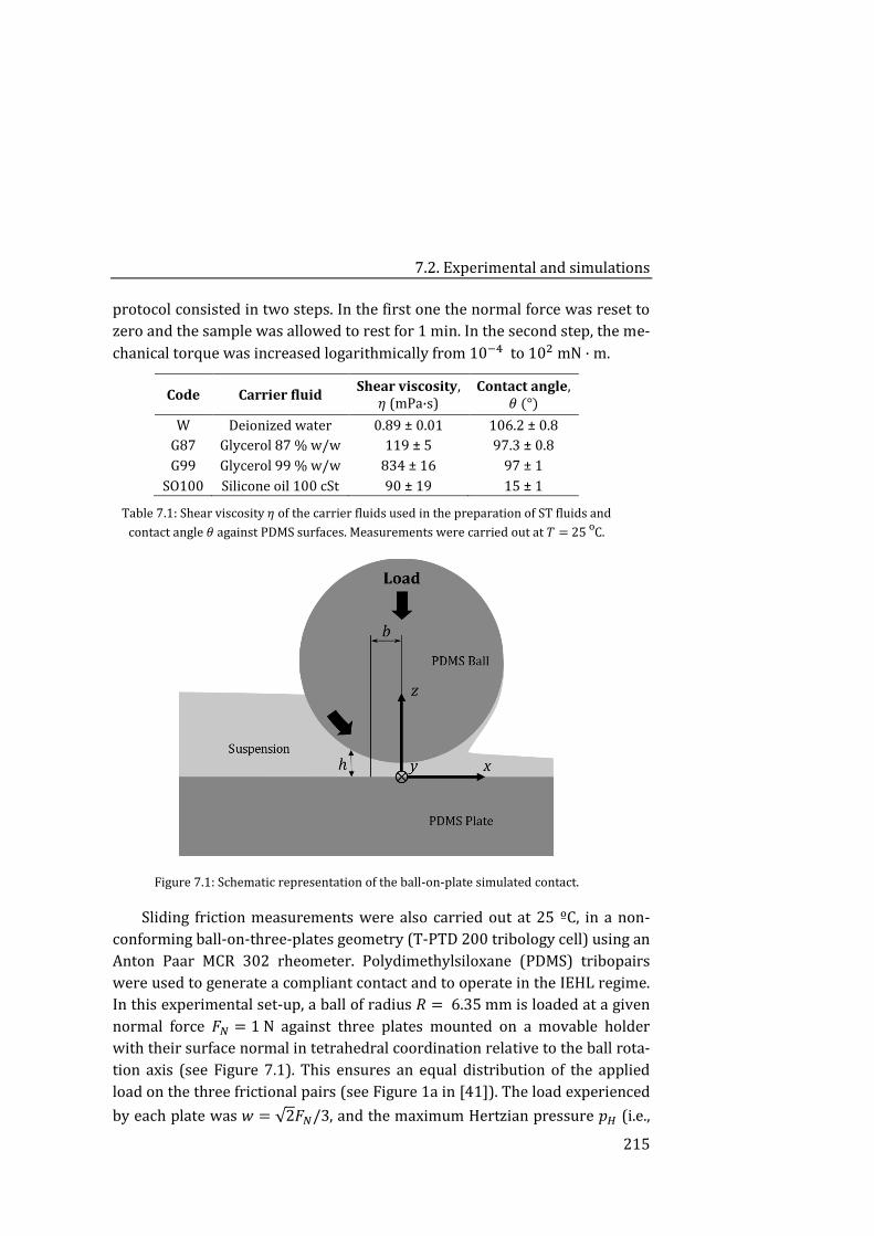
7.2. Experimental and simulations
215
protocol consisted in two steps. In the first one the normal force was reset to
zero and the sample was allowed to rest for 1 min. In the second step, the me-
chanical torque was increased logarithmically from 10−4 to 102 mN · m.
Code Carrier fluid Shear viscosity,
휂 (mPa·s) Contact angle,
휃 (°)
W Deionized water 0.89 ± 0.01 106.2 ± 0.8
G87 Glycerol 87 % w/w 119 ± 5 97.3 ± 0.8
G99 Glycerol 99 % w/w 834 ± 16 97 ± 1
SO100 Silicone oil 100 cSt 90 ± 19 15 ± 1
Table 7.1: Shear viscosity 휂 of the carrier fluids used in the preparation of ST fluids and
contact angle 휃 against PDMS surfaces. Measurements were carried out at 𝑇 = 25 ºC.
Figure 7.1: Schematic representation of the ball-on-plate simulated contact.
Sliding friction measurements were also carried out at 25 ºC, in a non-
conforming ball-on-three-plates geometry (T-PTD 200 tribology cell) using an
Anton Paar MCR 302 rheometer. Polydimethylsiloxane (PDMS) tribopairs
were used to generate a compliant contact and to operate in the IEHL regime.
In this experimental set-up, a ball of radius 𝑅 = 6.35 mm is loaded at a given
normal force 𝐹𝑁 = 1 N against three plates mounted on a movable holder
with their surface normal in tetrahedral coordination relative to the ball rota-
tion axis (see Figure 7.1). This ensures an equal distribution of the applied
load on the three frictional pairs (see Figure 1a in [41]). The load experienced
by each plate was 𝑤 = √2𝐹𝑁/3, and the maximum Hertzian pressure 𝑝𝐻 (i.e.,
7. Soft lubrication of cornstarch-based shear-thickening fluids
216
at the contact center) was 0.15 MPa [41]. It is obtained as 𝑝𝐻 =3𝑤
2𝜋𝑎𝑏 , where 𝑎
and 𝑏 are the major and minor axis in the Hertzian elliptical contact [42]. The
balls and plates were prepared in situ using conventional techniques from a
two-component silicone elastomer kit (SylgardTM 184, Dow Corning). PDMS
components have a Young’s modulus of 1.84 MPa, Poisson’s ratio of 0.5
[41,43] and hardness (Shore A) of 46.68 [44]. Once the sample was added in-
to the geometry, the ball was lowered to the measurement position. Then, the
normal force was adjusted to the commanded value during 1 min. In a second
step, the normal force was kept at the desired value and the ball was rotated
at a logarithmically increasing sliding speed (𝑉) from 5 · 10−4 to 1 m · s−1
during 5 minutes.
In order to get reproducible results a thorough cleaning procedure was
implemented. After every test, the sample was removed with paper and de-
ionized water, and all the pieces (ball, plates and holder) were dismounted
and carefully cleaned with ethanol. The PDMS ball and three plates were re-
placed when a different batch of samples had to be measured, i.e., when a dif-
ferent carrier fluid was employed. Also, after every test, the plates were care-
fully inspected for worn spots. The plates were also replaced when a worn
spot appeared on the surfaces. Both rheological and tribological tests were
carried out with fresh new samples in order to avoid water evaporation and
changes in the particle volume fraction. As it will be shown later this was es-
pecially important in the case of the G87-based suspensions (see Figure S2).
Experimental data reported here were obtained from sample averaging over
at least two repetitions.
Simulations were also performed to calculate the friction coefficient in
the IEHL regime. A detailed explanation of the simulation approach is given in
Subsection 3.3.4. The generalized Reynolds equation (Equation 3.46) governs
the flow behaviour in thin lubricated films [45–47]. Its numerical solution in-
volves the determination of the pressure distribution 𝑝(𝑥, 𝑦) and the film
thickness ℎ(𝑥, 𝑦) in the contact. In shear thickening fluids the viscosity in-
creases with the shear rate, and this dependency is well captured by the Car-
reau-Yasuda model (Equation 3.51) as constitutive equation. In a typical sim-
ulation the gap profile and pressure distribution are not uniform. As a result,
at a given sliding velocity, the shear rate at each point within the contact re-
gion changes, and so does the viscosity. Hence, at each node within the solu-
tion domain, the viscosity was obtained iteratively across the fluid film using
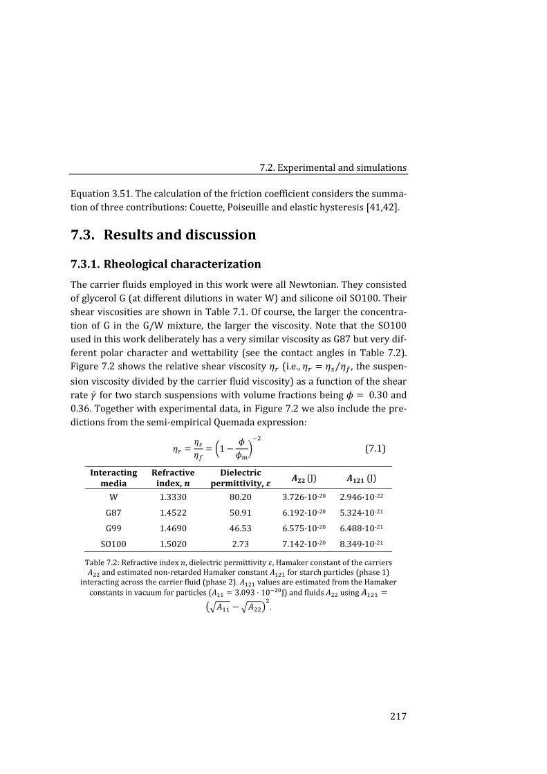
7.2. Experimental and simulations
217
Equation 3.51. The calculation of the friction coefficient considers the summa-
tion of three contributions: Couette, Poiseuille and elastic hysteresis [41,42].
7.3. Results and discussion
7.3.1. Rheological characterization
The carrier fluids employed in this work were all Newtonian. They consisted
of glycerol G (at different dilutions in water W) and silicone oil SO100. Their
shear viscosities are shown in Table 7.1. Of course, the larger the concentra-
tion of G in the G/W mixture, the larger the viscosity. Note that the SO100
used in this work deliberately has a very similar viscosity as G87 but very dif-
ferent polar character and wettability (see the contact angles in Table 7.2).
Figure 7.2 shows the relative shear viscosity 휂𝑟 (i.e., 휂𝑟 = 휂𝑠 휂𝑓⁄ , the suspen-
sion viscosity divided by the carrier fluid viscosity) as a function of the shear
rate �̇� for two starch suspensions with volume fractions being 𝜙 = 0.30 and
0.36. Together with experimental data, in Figure 7.2 we also include the pre-
dictions from the semi-empirical Quemada expression:
휂𝑟 =휂𝑠
휂𝑓
= (1 −𝜙
𝜙𝑚
)−2
(7.1)
Interacting media
Refractive index, 𝒏
Dielectric permittivity, 𝜺
𝑨𝟐𝟐 (J) 𝑨𝟏𝟐𝟏 (J)
W 1.3330 80.20 3.726·10-20 2.946·10-22
G87 1.4522 50.91 6.192·10-20 5.324·10-21
G99 1.4690 46.53 6.575·10-20 6.488·10-21
SO100 1.5020 2.73 7.142·10-20 8.349·10-21
Table 7.2: Refractive index 𝑛, dielectric permittivity 휀, Hamaker constant of the carriers 𝐴22 and estimated non-retarded Hamaker constant 𝐴121 for starch particles (phase 1)
interacting across the carrier fluid (phase 2). 𝐴121 values are estimated from the Hamaker
constants in vacuum for particles (𝐴11 = 3.093 · 10−20J) and fluids 𝐴22 using 𝐴121 =
(√𝐴11 − √𝐴22)2
.
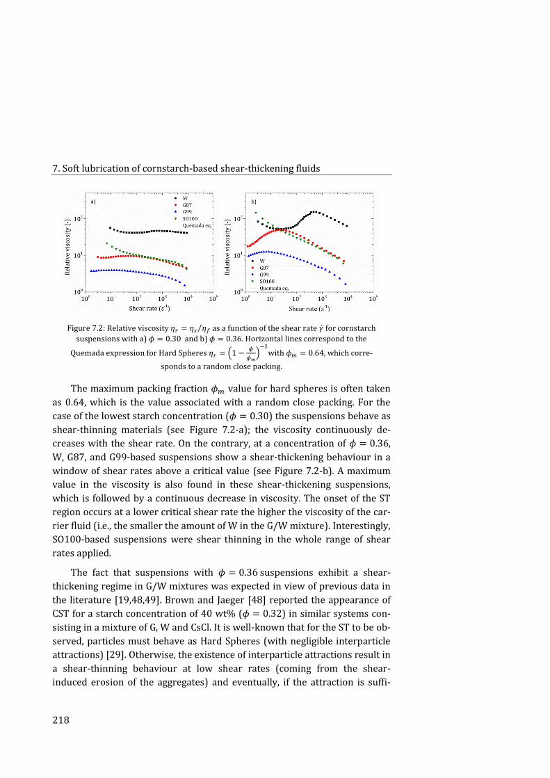
7. Soft lubrication of cornstarch-based shear-thickening fluids
218
Figure 7.2: Relative viscosity 휂𝑟 = 휂𝑠 휂𝑓⁄ as a function of the shear rate �̇� for cornstarch
suspensions with a) 𝜙 = 0.30 and b) 𝜙 = 0.36. Horizontal lines correspond to the
Quemada expression for Hard Spheres 휂𝑟 = (1 −𝜙
𝜙𝑚)
−2with 𝜙𝑚 = 0.64, which corre-
sponds to a random close packing.
The maximum packing fraction 𝜙𝑚 value for hard spheres is often taken
as 0.64, which is the value associated with a random close packing. For the
case of the lowest starch concentration (𝜙 = 0.30) the suspensions behave as
shear-thinning materials (see Figure 7.2-a); the viscosity continuously de-
creases with the shear rate. On the contrary, at a concentration of 𝜙 = 0.36,
W, G87, and G99-based suspensions show a shear-thickening behaviour in a
window of shear rates above a critical value (see Figure 7.2-b). A maximum
value in the viscosity is also found in these shear-thickening suspensions,
which is followed by a continuous decrease in viscosity. The onset of the ST
region occurs at a lower critical shear rate the higher the viscosity of the car-
rier fluid (i.e., the smaller the amount of W in the G/W mixture). Interestingly,
SO100-based suspensions were shear thinning in the whole range of shear
rates applied.
The fact that suspensions with 𝜙 = 0.36 suspensions exhibit a shear-
thickening regime in G/W mixtures was expected in view of previous data in
the literature [19,48,49]. Brown and Jaeger [48] reported the appearance of
CST for a starch concentration of 40 wt% (𝜙 = 0.32) in similar systems con-
sisting in a mixture of G, W and CsCl. It is well-known that for the ST to be ob-
served, particles must behave as Hard Spheres (with negligible interparticle
attractions) [29]. Otherwise, the existence of interparticle attractions result in
a shear-thinning behaviour at low shear rates (coming from the shear-
induced erosion of the aggregates) and eventually, if the attraction is suffi-
7.3. Results and discussion
219
ciently large, to the appearance of a yield stress that may hide the shear
thickening phenomenon [6,7,9,29].
In the systems investigated in this work, interparticle attractions are nec-
essarily present as a result of van der Waals forces that, in their turn, depend
on the non-retarded Hamaker constant. Estimations of the non-retarded
Hamaker constant 𝐴121 for two cornstarch particles (phase 1) separated by a
carrier fluid (phase 2) are shown in Table 7.2. The value of the Hamaker con-
stant for cornstarch in vacuum 𝐴11 = 3.093 · 10−20 J was obtained from
measurements of adhesive forces [50], while the values for the carrier fluids
𝐴22 were calculated from the refractive indexes and dielectric permittivities
of the carriers found in the literature [51]. The non-retarded Hamaker con-
stant is then obtained from 𝐴121 = (√𝐴11 − √𝐴22)2
. Differences observed in
the shear-thickening response between the carrier fluids employed in this
work can be explained in terms of interparticle interactions. In brief, pure wa-
ter based suspensions exhibit the smaller 𝐴121 values and concomitantly the
stronger shear thickening effect. This is in agreement with the hydrocluster
mechanism proposed by Brady and coworkers. Upon the addition of glycerol,
interparticle attractions are promoted (i.e., 𝐴121 increases) and the critical
rate for shear thickening is shifted to lower values (see Figure 7.2-b). Finally,
SO100-based suspensions exhibit the stronger interparticle attractions (larg-
er 𝐴121 values). In these particular suspensions the viscosity diverges at low
shear rates (i.e., a slope of -1 is envisaged in Figure 7.2-b at low shear rates) in
agreement with the appearance of a yield stress that overcomes the critical
stress for shear thickening. As a result the shear thickening is masked. Apart
from this qualitative explanation in terms of the hydrocluster mechanism, it is
important to remark that a more efficient electrostatic stabilization in G/W
mixtures is also expected since hydroxyl groups available onto the starch par-
ticles could form hydrogen bonds with polar molecules in G/W carriers
[52,53].
7.3.2. Tribological characterization
Figure 7.3-a shows the friction coefficient 𝜇 as a function of the sliding speed
𝑉 for the four different carrier fluids investigated (without particles). Regard-
less the nature of each particular liquid, three regions are identified. At low
speed, the friction is essentially constant and originates from the interaction
between the two surfaces (boundary friction). With increasing speed the fluid
partially fills the space between both surfaces so that they are pushed apart
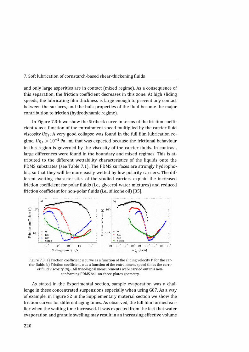
7. Soft lubrication of cornstarch-based shear-thickening fluids
220
and only large asperities are in contact (mixed regime). As a consequence of
this separation, the friction coefficient decreases in this zone. At high sliding
speeds, the lubricating film thickness is large enough to prevent any contact
between the surfaces, and the bulk properties of the fluid become the major
contribution to friction (hydrodynamic regime).
In Figure 7.3-b we show the Stribeck curve in terms of the friction coeffi-
cient 𝜇 as a function of the entrainment speed multiplied by the carrier fluid
viscosity 𝑈휂𝑓 . A very good collapse was found in the full film lubrication re-
gime, 𝑈휂𝑓 > 10−2 Pa · m, that was expected because the frictional behaviour
in this region is governed by the viscosity of the carrier fluids. In contrast,
large differences were found in the boundary and mixed regimes. This is at-
tributed to the different wettability characteristics of the liquids onto the
PDMS substrates (see Table 7.1). The PDMS surfaces are strongly hydropho-
bic, so that they will be more easily wetted by low polarity carriers. The dif-
ferent wetting characteristics of the studied carriers explain the increased
friction coefficient for polar fluids (i.e., glycerol-water mixtures) and reduced
friction coefficient for non-polar fluids (i.e., silicone oil) [35].
Figure 7.3: a) Friction coefficient 𝜇 curve as a function of the sliding velocity 𝑉 for the car-rier fluids. b) Friction coefficient 𝜇 as a function of the entrainment speed times the carri-
er fluid viscosity 𝑈휂𝑓 . All tribological measurements were carried out in a non-
conforming PDMS ball-on-three-plates geometry.
As stated in the Experimental section, sample evaporation was a chal-
lenge in these concentrated suspensions especially when using G87. As a way
of example, in Figure S2 in the Supplementary material section we show the
friction curves for different aging times. As observed, the full film formed ear-
lier when the waiting time increased. It was expected from the fact that water
evaporation and granule swelling may result in an increasing effective volume
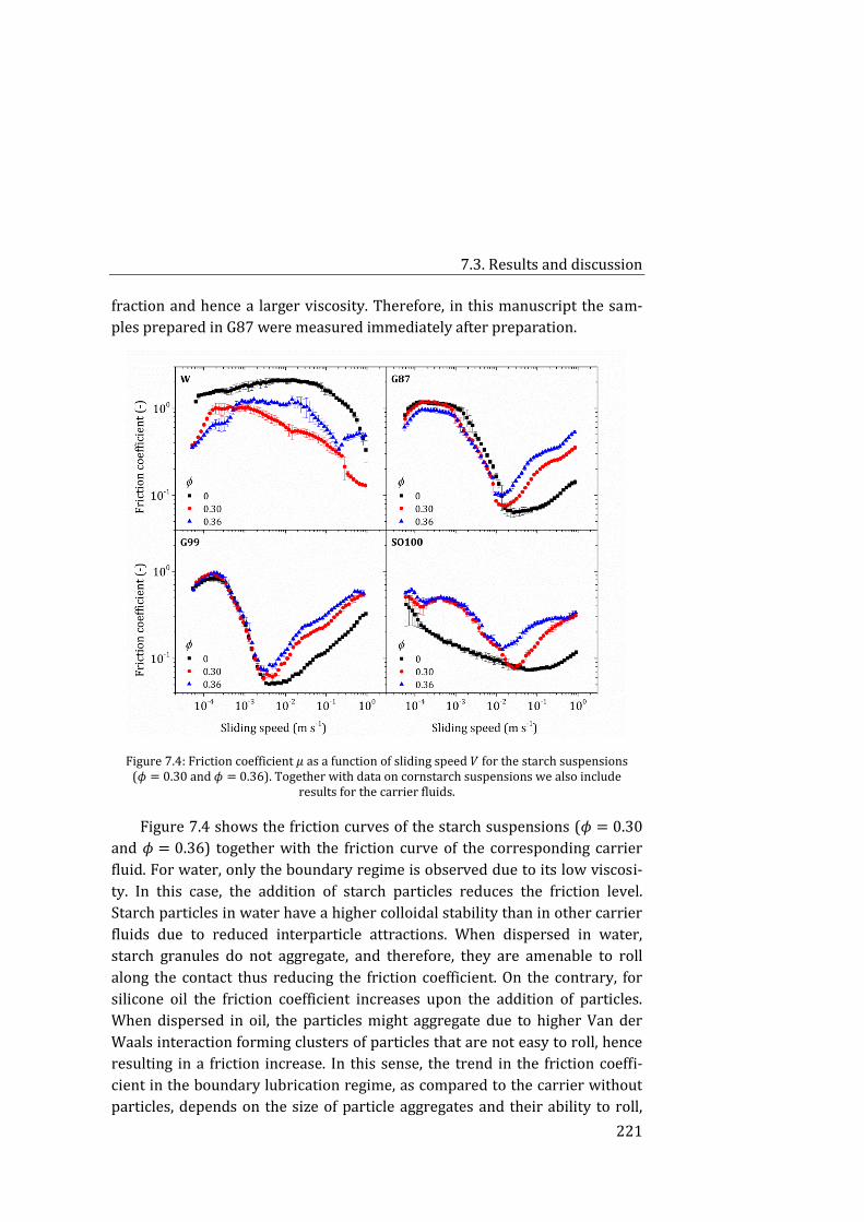
7.3. Results and discussion
221
fraction and hence a larger viscosity. Therefore, in this manuscript the sam-
ples prepared in G87 were measured immediately after preparation.
Figure 7.4: Friction coefficient 𝜇 as a function of sliding speed 𝑉 for the starch suspensions (𝜙 = 0.30 and 𝜙 = 0.36). Together with data on cornstarch suspensions we also include
results for the carrier fluids.
Figure 7.4 shows the friction curves of the starch suspensions (𝜙 = 0.30
and 𝜙 = 0.36) together with the friction curve of the corresponding carrier
fluid. For water, only the boundary regime is observed due to its low viscosi-
ty. In this case, the addition of starch particles reduces the friction level.
Starch particles in water have a higher colloidal stability than in other carrier
fluids due to reduced interparticle attractions. When dispersed in water,
starch granules do not aggregate, and therefore, they are amenable to roll
along the contact thus reducing the friction coefficient. On the contrary, for
silicone oil the friction coefficient increases upon the addition of particles.
When dispersed in oil, the particles might aggregate due to higher Van der
Waals interaction forming clusters of particles that are not easy to roll, hence
resulting in a friction increase. In this sense, the trend in the friction coeffi-
cient in the boundary lubrication regime, as compared to the carrier without
particles, depends on the size of particle aggregates and their ability to roll,
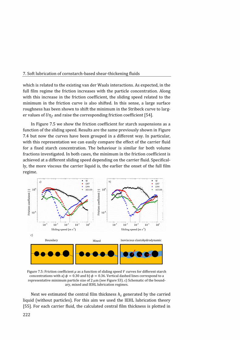
7. Soft lubrication of cornstarch-based shear-thickening fluids
222
which is related to the existing van der Waals interactions. As expected, in the
full film regime the friction increases with the particle concentration. Along
with this increase in the friction coefficient, the sliding speed related to the
minimum in the friction curve is also shifted. In this sense, a large surface
roughness has been shown to shift the minimum in the Stribeck curve to larg-
er values of 𝑈휂𝑓 and raise the corresponding friction coefficient [54].
In Figure 7.5 we show the friction coefficient for starch suspensions as a
function of the sliding speed. Results are the same previously shown in Figure
7.4 but now the curves have been grouped in a different way. In particular,
with this representation we can easily compare the effect of the carrier fluid
for a fixed starch concentration. The behaviour is similar for both volume
fractions investigated. In both cases, the minimum in the friction coefficient is
achieved at a different sliding speed depending on the carrier fluid. Specifical-
ly, the more viscous the carrier liquid is, the earlier the onset of the full film
regime.
Figure 7.5: Friction coefficient 𝜇 as a function of sliding speed 𝑉 curves for different starch concentrations with a) 𝜙 = 0.30 and b) 𝜙 = 0.36. Vertical dashed lines correspond to a
representative minimum particle size of 2 m (see Figure S3). c) Schematic of the bound-ary, mixed and IEHL lubrication regimes.
Next we estimated the central film thickness ℎ𝑐 generated by the carried
liquid (without particles). For this aim we used the IEHL lubrication theory
[55]. For each carrier fluid, the calculated central film thickness is plotted in
7.3. Results and discussion
223
Figure S3 in the Supplementary material section as a function of the sliding
speed. Horizontal/vertical lines in Figure S3 correspond to representative
film thicknesses (2, 5 and 8 μm)/sliding speeds. The vertical lines in Figure
7.5 correspond to the critical speeds identified in Figure S3 for a central film
thickness of 2 µm. It can be observed that the speeds corresponding to a cen-
tral film thickness of 2 µm are very close to the critical sliding speeds corre-
sponding to the minimum in the friction curves. This suggests that, as a first
approximation, the minimum in the friction coefficient is correlated with the
viscosity of the carrier fluid. Later, in subsection 7.3.3 we will see that a more
appropriate description is given by the suspension viscosity instead of the
carrier fluid viscosity.
In an attempt to rationalize the central film thickness associated to the
minimum in the Stribeck curve, we performed a thorough particle size analy-
sis. Starch particles used in this work are highly polydisperse as shown in
Figure S1 in the Supplementary material section. If a normal distribution is
considered, the minimum particle diameter is approximately given by
𝜇𝑚 − 3𝜎𝑚, being 𝜇𝑚 = 10.7 μm the average diameter and 𝜎𝑚 = 3.3 μm the
standard deviation. With this, the minimum particle diameter is approximate-
ly 1-2 μm, which is very close to that obtained from IEHL lubrication calcula-
tions. As a result, the minimum in Figure 7.5 can be interpreted as follows:
below the critical speed, associated to the minimum in the friction coefficient,
particles are not allowed to pass through the contact. However, above the
critical speed the gap is sufficiently large for most of the particles to pass
through (see Subsection 7.2.4). This suggests that the corresponding sliding
speed to the minimum in the friction coefficient is associated to the (mini-
mum) particle size. This explanation is summarized in the schematic in Figure
7.5.
Next, we constructed the Stribeck curves by multiplying the entrainment
speed by the shear viscosity of the carrier fluid (without particles) -and not
by that of the particular suspension that changes with the shear rate-. These
results are shown in Figure 7.6. The fact that the curves collapse in the mixed
lubrication regime demonstrates that the transition from the boundary to the
mixed regime is dictated by the viscosity of the carrier liquid, hence suggest-
ing that in the boundary regime the particles simply roll when the ball slides
above the plates, and that in the transition to the mixed regime the carrier
liquid is capable to be entrained in the contact (see schematics in Figure 7.5).
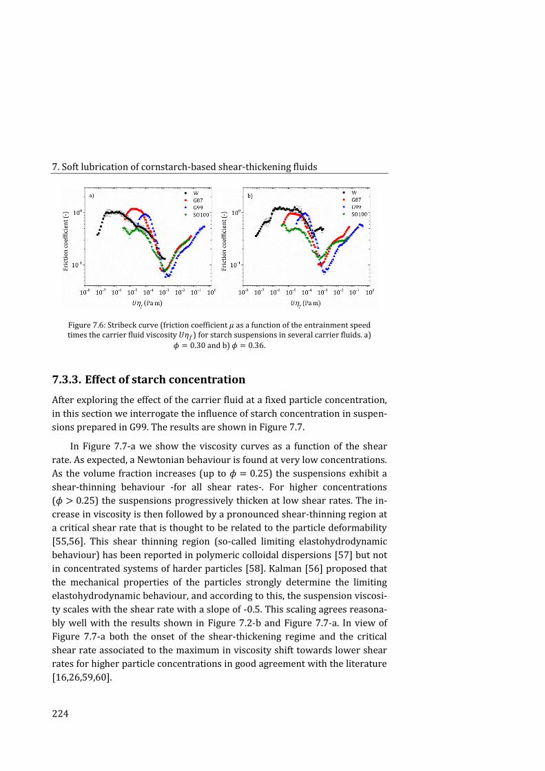
7. Soft lubrication of cornstarch-based shear-thickening fluids
224
Figure 7.6: Stribeck curve (friction coefficient 𝜇 as a function of the entrainment speed times the carrier fluid viscosity 𝑈휂𝑓) for starch suspensions in several carrier fluids. a)
𝜙 = 0.30 and b) 𝜙 = 0.36.
7.3.3. Effect of starch concentration
After exploring the effect of the carrier fluid at a fixed particle concentration,
in this section we interrogate the influence of starch concentration in suspen-
sions prepared in G99. The results are shown in Figure 7.7.
In Figure 7.7-a we show the viscosity curves as a function of the shear
rate. As expected, a Newtonian behaviour is found at very low concentrations.
As the volume fraction increases (up to 𝜙 = 0.25) the suspensions exhibit a
shear-thinning behaviour -for all shear rates-. For higher concentrations
(𝜙 > 0.25) the suspensions progressively thicken at low shear rates. The in-
crease in viscosity is then followed by a pronounced shear-thinning region at
a critical shear rate that is thought to be related to the particle deformability
[55,56]. This shear thinning region (so-called limiting elastohydrodynamic
behaviour) has been reported in polymeric colloidal dispersions [57] but not
in concentrated systems of harder particles [58]. Kalman [56] proposed that
the mechanical properties of the particles strongly determine the limiting
elastohydrodynamic behaviour, and according to this, the suspension viscosi-
ty scales with the shear rate with a slope of -0.5. This scaling agrees reasona-
bly well with the results shown in Figure 7.2-b and Figure 7.7-a. In view of
Figure 7.7-a both the onset of the shear-thickening regime and the critical
shear rate associated to the maximum in viscosity shift towards lower shear
rates for higher particle concentrations in good agreement with the literature
[16,26,59,60].
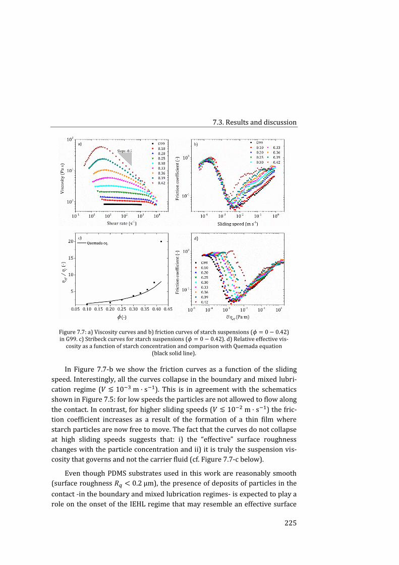
7.3. Results and discussion
225
Figure 7.7: a) Viscosity curves and b) friction curves of starch suspensions (𝜙 = 0 − 0.42) in G99. c) Stribeck curves for starch suspensions (𝜙 = 0 − 0.42). d) Relative effective vis-
cosity as a function of starch concentration and comparison with Quemada equation (black solid line).
In Figure 7.7-b we show the friction curves as a function of the sliding
speed. Interestingly, all the curves collapse in the boundary and mixed lubri-
cation regime (𝑉 ≲ 10−3 m · s−1). This is in agreement with the schematics
shown in Figure 7.5: for low speeds the particles are not allowed to flow along
the contact. In contrast, for higher sliding speeds (𝑉 ≲ 10−2 m · s−1) the fric-
tion coefficient increases as a result of the formation of a thin film where
starch particles are now free to move. The fact that the curves do not collapse
at high sliding speeds suggests that: i) the “effective” surface roughness
changes with the particle concentration and ii) it is truly the suspension vis-
cosity that governs and not the carrier fluid (cf. Figure 7.7-c below).
Even though PDMS substrates used in this work are reasonably smooth
(surface roughness 𝑅𝑞 < 0.2 μm), the presence of deposits of particles in the
contact -in the boundary and mixed lubrication regimes- is expected to play a
role on the onset of the IEHL regime that may resemble an effective surface
7. Soft lubrication of cornstarch-based shear-thickening fluids
226
roughness. The influence of surface roughness in soft tribology has been de-
scribed in the literature [54]. In the case of rough surfaces, the transition from
the mixed to the IEHL regime occurs for lower values of the film thickness
parameter at smaller sliding speeds. A rougher contact is generated in this
work by simply increasing the particle concentration. As a result, it is not sur-
prising that the onset of the IEHL regime occurs at smaller sliding speeds in
good agreement with Figure 7.7-b.
The literature demonstrates that the entrainment of particles in suspen-
sion play a crucial role in the IEHL regime. Dwyer-Joyce and Heymcr [61] and
Yakubov et al. [37] showed how particles of different size behaved in and
around EHL contacts. In rolling motion, the friction forces on the particles in
the inlet zone provokes its drag through the contact, whereas in sliding mo-
tion the particles tends to rotate as a consequence of a friction couple [62].
For pure sliding, most particles tend to accumulate in the inlet to cause star-
vation. Timm et al. [63] found that in fully flooded contacts, the addition of
particles to a carrier liquid had no significant effect on the friction level be-
cause very few particles could pass through the contact (only particles close
to central streamline would enter the contact). However, for partially lubri-
cated contacts particles appeared to concentrate around the contact region. In
summary, the dependence of the hydrodynamic transition speed with concen-
tration suggests that a layer of deformed starch particles is likely to form at
the contact hence modifying the effective surface roughness.
To obtain an estimate of the effective viscosity of the suspension being
entrained in the contact, values have been calculated by forcing the Stribeck
curves to collapse within the hydrodynamic regime on a master curve. The
master curve is shown in Figure 7.7-c. These effective viscosity values, denot-
ed as 휂𝑒𝑓𝑓, were compared to Quemada equation in Figure 7.7-d. The calcu-
lated viscosity and theoretical predictions are in a good agreement up to
𝜙 = 0.39. Only for 𝜙 = 0.42 a large deviation was observed from the theoreti-
cal prediction. This suggests that the rheological response of the thin film
formed between the PDMS surfaces could be assimilated as a suspension of
hard spheres.
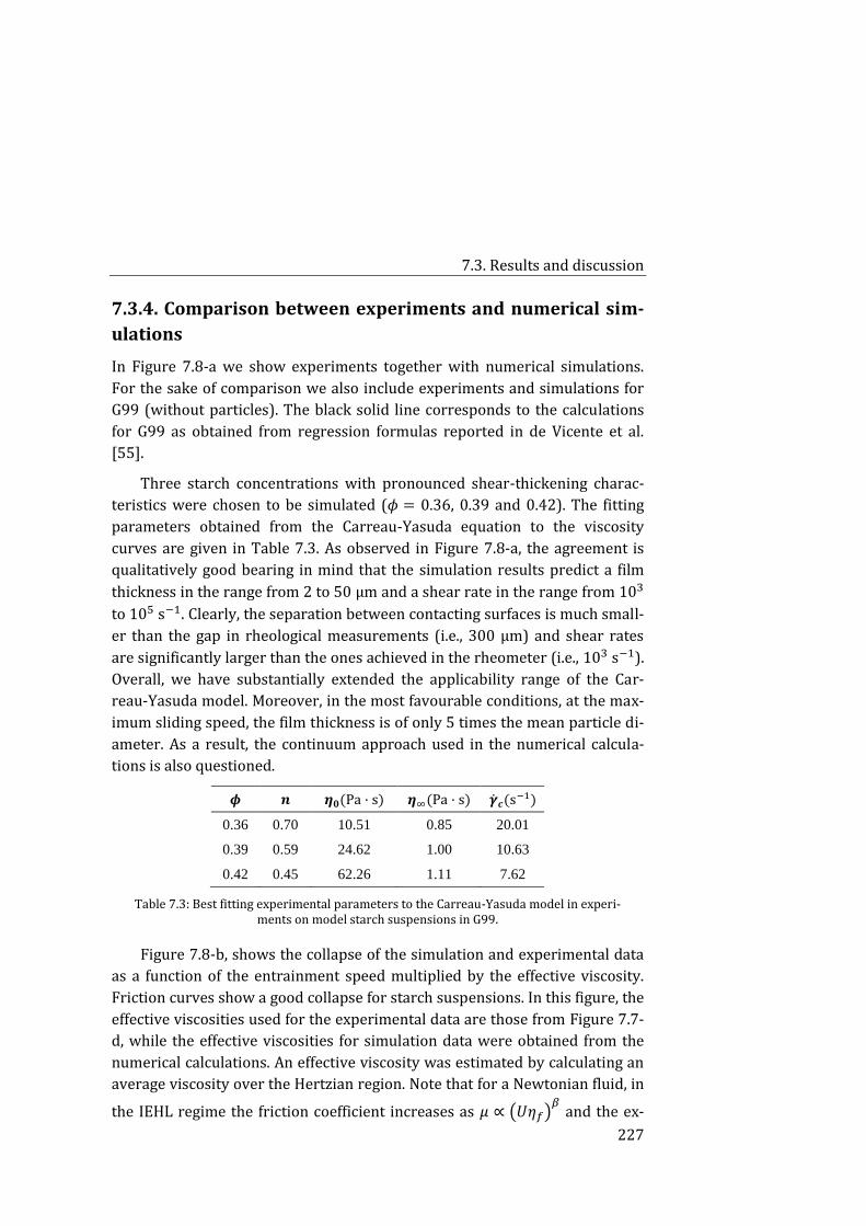
7.3. Results and discussion
227
7.3.4. Comparison between experiments and numerical sim-
ulations
In Figure 7.8-a we show experiments together with numerical simulations.
For the sake of comparison we also include experiments and simulations for
G99 (without particles). The black solid line corresponds to the calculations
for G99 as obtained from regression formulas reported in de Vicente et al.
[55].
Three starch concentrations with pronounced shear-thickening charac-
teristics were chosen to be simulated (𝜙 = 0.36, 0.39 and 0.42). The fitting
parameters obtained from the Carreau-Yasuda equation to the viscosity
curves are given in Table 7.3. As observed in Figure 7.8-a, the agreement is
qualitatively good bearing in mind that the simulation results predict a film
thickness in the range from 2 to 50 μm and a shear rate in the range from 103
to 105 s−1. Clearly, the separation between contacting surfaces is much small-
er than the gap in rheological measurements (i.e., 300 μm) and shear rates
are significantly larger than the ones achieved in the rheometer (i.e., 103 s−1).
Overall, we have substantially extended the applicability range of the Car-
reau-Yasuda model. Moreover, in the most favourable conditions, at the max-
imum sliding speed, the film thickness is of only 5 times the mean particle di-
ameter. As a result, the continuum approach used in the numerical calcula-
tions is also questioned.
𝝓 𝒏 𝜼𝟎(Pa · s) 𝜼∞(Pa · s) �̇�𝒄(s−1)
0.36 0.70 10.51 0.85 20.01
0.39 0.59 24.62 1.00 10.63
0.42 0.45 62.26 1.11 7.62
Table 7.3: Best fitting experimental parameters to the Carreau-Yasuda model in experi-ments on model starch suspensions in G99.
Figure 7.8-b, shows the collapse of the simulation and experimental data
as a function of the entrainment speed multiplied by the effective viscosity.
Friction curves show a good collapse for starch suspensions. In this figure, the
effective viscosities used for the experimental data are those from Figure 7.7-
d, while the effective viscosities for simulation data were obtained from the
numerical calculations. An effective viscosity was estimated by calculating an
average viscosity over the Hertzian region. Note that for a Newtonian fluid, in
the IEHL regime the friction coefficient increases as 𝜇 ∝ (𝑈휂𝑓)𝛽
and the ex-
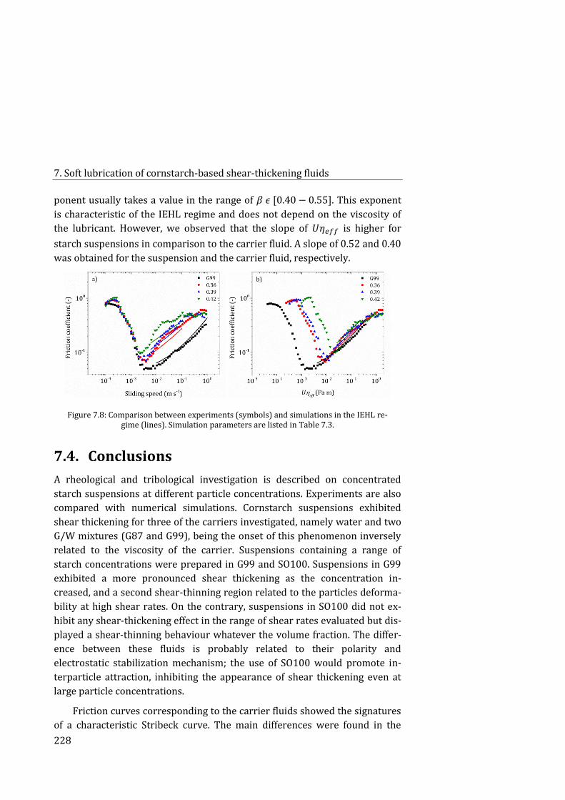
7. Soft lubrication of cornstarch-based shear-thickening fluids
228
ponent usually takes a value in the range of 𝛽 𝜖 [0.40 − 0.55]. This exponent
is characteristic of the IEHL regime and does not depend on the viscosity of
the lubricant. However, we observed that the slope of 𝑈휂𝑒𝑓𝑓 is higher for
starch suspensions in comparison to the carrier fluid. A slope of 0.52 and 0.40
was obtained for the suspension and the carrier fluid, respectively.
Figure 7.8: Comparison between experiments (symbols) and simulations in the IEHL re-gime (lines). Simulation parameters are listed in Table 7.3.
7.4. Conclusions
A rheological and tribological investigation is described on concentrated
starch suspensions at different particle concentrations. Experiments are also
compared with numerical simulations. Cornstarch suspensions exhibited
shear thickening for three of the carriers investigated, namely water and two
G/W mixtures (G87 and G99), being the onset of this phenomenon inversely
related to the viscosity of the carrier. Suspensions containing a range of
starch concentrations were prepared in G99 and SO100. Suspensions in G99
exhibited a more pronounced shear thickening as the concentration in-
creased, and a second shear-thinning region related to the particles deforma-
bility at high shear rates. On the contrary, suspensions in SO100 did not ex-
hibit any shear-thickening effect in the range of shear rates evaluated but dis-
played a shear-thinning behaviour whatever the volume fraction. The differ-
ence between these fluids is probably related to their polarity and
electrostatic stabilization mechanism; the use of SO100 would promote in-
terparticle attraction, inhibiting the appearance of shear thickening even at
large particle concentrations.
Friction curves corresponding to the carrier fluids showed the signatures
of a characteristic Stribeck curve. The main differences were found in the
7.4. Conclusions
229
boundary region, where friction increased with the carrier polarity, as it pro-
vides a different wettability on the hydrophobic PDMS plates. The critical slid-
ing speed at the minimum friction coefficient evolved as expected; it shifted to
lower values with increasing the fluid viscosity. The addition of cornstarch
particles showed an increase in friction in the hydrodynamic region for all the
carriers. However, the effect of the addition of particles in the boundary fric-
tion coefficient differs for each carrier, due to different van der Waals interac-
tions. In the case of water (a highly polar carrier), the addition of particles
reduced friction as compared to the friction curve of the carrier, while for
SO100 (a non-polar carrier) their tribological behaviour was opposed and
friction coefficient increased. This suggests that the particle-fluid interactions
greatly affect the response; in water, starch particles would simply roll, while
in SO100, the interparticle attraction would lead to the formation of aggre-
gates. These aggregates would act as asperities in such small contact, leading
to a friction increase with particle concentration in this region. For G99-based
suspensions, friction curves collapse in the boundary lubrication and mixed
regimes whatever the concentration, what suggests that only the carrier fluid
goes through the contact at slow sliding speeds. On the other hand, if Stribeck
curves are constructed and forced to collapse in the IEHL regime, the critical
friction increases and shifts to higher values of 𝑈휂𝑒𝑓𝑓 with the suspension
concentration. This shift was also observed to happen when the surface
roughness is modified. In the present work it is attributed to a layer of de-
formed starch particles at the contact, hence effectively roughening the PDMS
surfaces. Numerical simulations in the IEHL regime were compared with
tribological experiments of G99-based starch suspensions. The agreement
was not as good for suspensions as for the Newtonian carrier fluids without
particles. This discrepancy is thought to be due to the formation of a different
microstructure in rheological and tribological tests.
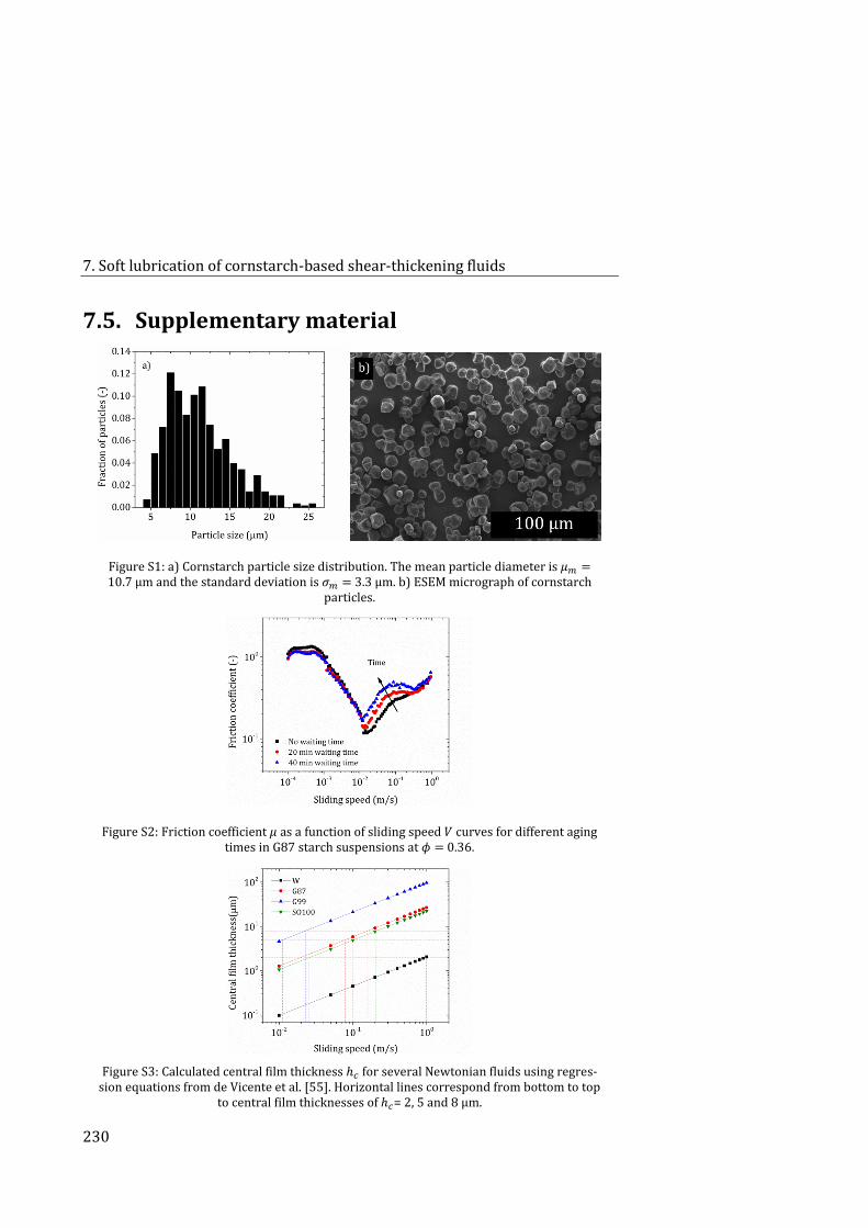
7. Soft lubrication of cornstarch-based shear-thickening fluids
230
7.5. Supplementary material
Figure S1: a) Cornstarch particle size distribution. The mean particle diameter is 𝜇𝑚 = 10.7 μm and the standard deviation is 𝜎𝑚 = 3.3 μm. b) ESEM micrograph of cornstarch
particles.
Figure S2: Friction coefficient 𝜇 as a function of sliding speed 𝑉 curves for different aging times in G87 starch suspensions at 𝜙 = 0.36.
Figure S3: Calculated central film thickness ℎ𝑐 for several Newtonian fluids using regres-sion equations from de Vicente et al. [55]. Horizontal lines correspond from bottom to top
to central film thicknesses of ℎ𝑐= 2, 5 and 8 μm.
7.6. References
231
7.6. References
[1] Macosko C W 1994 Rheology: principles, measurements, and applica-tions (New York: VCH)
[2] Denn M M, Morris J F and Bonn D 2018 Shear thickening in concen-trated suspensions of smooth spheres in Newtonian suspending fluids Soft Matter 14 170–184
[3] Shenoy S S, Wagner N J and Bender J W 2003 E-FiRST: Electric field responsive shear thickening fluids Rheol. Acta 42 287–294
[4] Lee Y S, Wetzel E D and Wagner N J 2003 The ballistic impact charac-teristics of Kevlar® woven fabrics impregnated with a colloidal shear thick-ening fluid J. Mater. Sci. 38 2825–2833
[5] Crawford N C, Williams S K R, Boldridge D and Liberatore M W 2012 Shear thickening of chemical mechanical polishing slurries under high shear Rheol. Acta 51 637–647
[6] Barnes H A 1989 Shear-thickening (“Dilatancy”) in suspensions of nonaggregating solid particles dispersed in Newtonian liquids J. Rheol. 33 329–366
[7] Gopalakrishnan V and Zukoski C F 2004 Effect of attractions on shear thickening in dense suspensions J. Rheol. 48 1321–1344
[8] Melrose J R and Ball R C 2004 Continuous shear thickening transi-tions in model concentrated colloids—The role of interparticle forces J. Rheol. 48 937–960
[9] Pednekar S, Chun J and Morris J F 2017 Simulation of shear thicken-ing in attractive colloidal suspensions Soft Matter 13 1773–1779
[10] Gamonpilas C, Morris J F and Denn M M 2016 Shear and normal stress measurements in non-Brownian monodisperse and bidisperse suspen-sions J. Rheol. 60 289–296
[11] Maranzano B J and Wagner N J 2001 The effects of particle size on re-versible shear thickening of concentrated colloidal dispersions J. Chem. Phys. 114 10514–10527
[12] Guy B M, Hermes M and Poon W C K 2015 Towards a unified descrip-tion of the rheology of hard-particle suspensions Phys. Rev. Lett. 115
[13] Brown E, Zhang H, Forman N A, Maynor B W, Betts D E, DeSimone J M and Jaeger H M 2011 Shear thickening and jamming in densely packed sus-pensions of different particle shapes Phys. Rev. E 84
7. Soft lubrication of cornstarch-based shear-thickening fluids
232
[14] Lootens D, Damme H van, Hémar Y and Hébraud P 2005 Dilatant flow of concentrated suspensions of rough particles Phys. Rev. Lett. 95
[15] Jamali S, Boromand A, Wagner N and Maia J 2015 Microstructure and rheology of soft to rigid shear-thickening colloidal suspensions J. Rheol. 59 1377–1395
[16] Hsiao L C, Jamali S, Glynos E, Green P F, Larson R G and Solomon M J 2017 Rheological state diagrams for rough colloids in shear flow Phys. Rev. Lett. 119
[17] Hsu C-P, Ramakrishna S N, Zanini M, Spencer N D and Isa L 2018 Roughness-dependent tribology effects on discontinuous shear thickening Proc. Natl. Acad. Sci. 115 5117–5122
[18] Antosik A, Gluszek M, Zurowski R and Szafran M 2017 Influence of carrier fluid on the electrokinetic and rheological properties of shear thicken-ing fluids Ceram. Int. 43 12293–12301
[19] Swarna, Pattanayek S K and Ghosh A K 2017 Role of hydrogen bond interactions in water–polyol medium in the thickening behavior of cornstarch suspensions Colloid Polym. Sci. 295 1117–1129
[20] Brown E and Jaeger H M 2014 Shear thickening in concentrated sus-pensions: phenomenology, mechanisms and relations to jamming Rep. Prog. Phys. 77 046602
[21] Hoffman R L 1974 Discontinuous and dilatant viscosity behavior in concentrated suspensions. II. Theory and experimental tests J. Colloid Inter-face Sci. 46 491–506
[22] Fall A, Huang N, Bertrand F, Ovarlez G and Bonn D 2008 Shear thick-ening of cornstarch suspensions as a reentrant jamming transition Phys. Rev. Lett. 100
[23] Brady J F and Bossis G 1985 The rheology of concentrated suspen-sions of spheres in simple shear flow by numerical simulation J. Fluid Mech. 155 105
[24] Fall A, Bertrand F, Hautemayou D, Mezière C, Moucheront P, Lemaître A and Ovarlez G 2015 Macroscopic discontinuous shear thickening versus lo-cal shear jamming in cornstarch Phys. Rev. Lett. 114
[25] Fernandez N, Mani R, Rinaldi D, Kadau D, Mosquet M, Lombois-Burger H, Cayer-Barrioz J, Herrmann H J, Spencer N D and Isa L 2013 Micro-scopic mechanism for shear thickening of non-Brownian suspensions Phys. Rev. Lett. 111
7.6. References
233
[26] Mari R, Seto R, Morris J F and Denn M M 2014 Shear thickening, fric-tionless and frictional rheologies in non-Brownian suspensions J. Rheol. 58 1693–1724
[27] Tian Y, Jiang J, Meng Y and Wen S 2010 A shear thickening phenome-non in magnetic field controlled-dipolar suspensions Appl. Phys. Lett. 97 151904
[28] Tian Y, Zhang M, Jiang J, Pesika N, Zeng H, Israelachvili J, Meng Y and Wen S 2011 Reversible shear thickening at low shear rates of electrorheologi-cal fluids under electric fields Phys. Rev. E 83
[29] Brown E, Forman N A, Orellana C S, Zhang H, Maynor B W, Betts D E, DeSimone J M and Jaeger H M 2010 Generality of shear thickening in dense suspensions Nat. Mater. 9 220–224
[30] Fall A, Bertrand F, Ovarlez G and Bonn D 2012 Shear thickening of cornstarch suspensions J. Rheol. 56 575–591
[31] Stokes J R, Boehm M W and Baier S K 2013 Oral processing, texture and mouthfeel: From rheology to tribology and beyond Curr. Opin. Colloid In-terface Sci. 18 349–359
[32] Chen J 2009 Food oral processing—A review Food Hydrocoll. 23 1–25
[33] Eliasson A-C 2004 Starch in food structure, function and applications (Cambridge: Woodhead Pub.)
[34] Myant C, Spikes H A and Stokes J R 2010 Influence of load and elastic properties on the rolling and sliding friction of lubricated compliant contacts Tribol. Int. 43 55–63
[35] de Vicente J, Stokes J R and Spikes H A 2006 Soft lubrication of model hydrocolloids Food Hydrocoll. 20 483–91
[36] Stokes J R, Macakova L, Chojnicka-Paszun A, Kruif C G de and Jongh H H J de 2011 Lubrication, adsorption, and rheology of aqueous polysaccharide solutions Langmuir 27 3474–3484
[37] Yakubov G E, Branfield T E, Bongaerts J H H and Stokes J R 2015 Tri-bology of particle suspensions in rolling-sliding soft contacts Biotribology 3 1–10
[38] Yakubov G E, Zhong L, Li M, Boehm M W, Xie F, Beattie D A, Halley P J and Stokes J R 2015 Lubrication of starch in ionic liquid–water mixtures: Sol-uble carbohydrate polymers form a boundary film on hydrophobic surfaces Carbohydr. Polym. 133 507–516
7. Soft lubrication of cornstarch-based shear-thickening fluids
234
[39] Morell P, Chen J and Fiszman S 2017 The role of starch and saliva in tribology studies and the sensory perception of protein-added yogurts Food Funct. 8 545–553
[40] Olivares M L, Shahrivar K and Vicente J de 2019 Soft lubrication char-acteristics of microparticulated whey proteins used as fat replacers in dairy systems J. Food Eng. 245 157–165
[41] Shahrivar K and de Vicente J 2014 Ferrofluid lubrication of compliant polymeric contacts: effect of non-homogeneous magnetic fields Tribol. Lett. 56 281–92
[42] Hamrock B, Schmid S and Jacobson B 2004 Fundamentals of fluid film lubrication (CRC Press)
[43] Bombard A J F, Gonçalves F R, Shahrivar K, Ortiz A L and Vicente J de 2015 Tribological behavior of ionic liquid-based magnetorheological fluids in steel and polymeric point contacts Tribol. Int. 81 309–320
[44] Johnston I D, McCluskey D K, Tan C K L and Tracey M C 2014 Mechan-ical characterization of bulk Sylgard 184 for microfluidics and microengineer-ing J. Micromechanics Microengineering 24 035017
[45] Dowson D 1962 A generalized Reynolds equation for fluid-film lubri-cation Int. J. Mech. Sci. 4 159–170
[46] Katyal P and Kumar P 2012 Central film thickness formula for shear thinning lubricants in EHL point contacts under pure rolling Tribol. Int. 48 113–121
[47] Katyal P and Kumar P 2014 New central film thickness equation for shear thinning lubricants in elastohydrodynamic lubricated rolling/sliding point contact conditions J. Tribol. 136 041504
[48] Brown E and Jaeger H M 2012 The role of dilation and confining stresses in shear thickening of dense suspensions J. Rheol. 56 875–923
[49] Hermes M, Guy B M, Poon W C K, Poy G, Cates M E and Wyart M 2016 Unsteady flow and particle migration in dense, non-Brownian suspensions J. Rheol. 60 905–916
[50] Shimada Y, Yonezawa Y, Sunada H, Nonaka R, Katou K and Morishita H 2000 The development of an apparatus for measuring the adhesive force between fine particles. J. Soc. Powder Technol. Jpn. 37 658–664
[51] Haynes W M 2014 Handbook of Chemistry and Physics (CRC Boca Ra-ton)
7.6. References
235
[52] Raghavan S R, Walls H J and Khan S A 2000 Rheology of silica disper-sions in organic liquids: new evidence for solvation forces dictated by hydro-gen bonding Langmuir 16 7920–7930
[53] Taylor S E 2013 Rheology and structure of cornstarch suspensions in water-poly(propylene glycol) mixtures J. Dispers. Sci. Technol. 34 887–897
[54] Bongaerts J H H, Fourtouni K and Stokes J R 2007 Soft-tribology: Lu-brication in a compliant PDMS–PDMS contact Tribol. Int. 40 1531–1542
[55] de Vicente J, Stokes J R and Spikes H A 2005 The frictional properties of Newtonian fluids in rolling–sliding soft-EHL contact Tribol. Lett. 20 273–86
[56] Dennis P. Kalman 2010 Microstructure and rheology of concentrated suspensions of near hard-sphere colloids (University of Delaware)
[57] Chatté G, Comtet J, Niguès A, Bocquet L, Siria A, Ducouret G, Lequeux F, Lenoir N, Ovarlez G and Colin A 2018 Shear thinning in non-Brownian sus-pensions Soft Matter 14 879–893
[58] Hoffman R L 1972 Discontinuous and dilatant viscosity behavior in concentrated suspensions. I. Observation of a flow instability Trans. Soc. Rhe-ol. 16 155–173
[59] Egres R G and Wagner N J 2005 The rheology and microstructure of acicular precipitated calcium carbonate colloidal suspensions through the shear thickening transition J. Rheol. 49 719–746
[60] Cwalina C D and Wagner N J 2014 Material properties of the shear-thickened state in concentrated near hard-sphere colloidal dispersions J. Rhe-ol. 58 949–967
[61] Dwyer-Joyce R S and Heymcr J 1996 The entrainment of solid parti-cles into rolling elastohydrodynamic contacts Tribology Series (Elsevier) pp 135–140
[62] Wan G T Y and Spikes H A 1988 The behavior of suspended solid par-ticles in rolling and sliding elastohydrodynamic contacts Tribol. Trans. 31 12–21
[63] Timm K, Myant C, Spikes H A and Grunze M 2011 Particulate lubri-cants in cosmetic applications Tribol. Int. 44 1695–1703

237
8. On the squeeze-strengthening effect
in magnetorheology
8.1. Introduction
Magnetorheological (MR) fluids are field-responsive materials composed of
magnetizable particles suspended in a non-magnetic carrier fluid. Soft mag-
netic materials with a high saturation magnetization and low coercivity (i.e.,
easily magnetized and demagnetized) are commonly used in the formulation
of MR fluids, as carbonyl iron particles [1–4]. Particles in MR suspensions
have micrometric size so that they present magnetic multi-domains. In the
absence of an applied external magnetic field the fluid displays a Newtonian
behaviour, while under the application of a magnetic field these domains
align, and dipolar interactions give rise to particle aggregation in the field di-
rection. The chains or columns of magnetic particles restrict the flow, result-
ing in a drastic increase in the viscosity of the suspension. Under these condi-
tions rheological properties of MR fluids are generally assumed to obey a
Bingham law. This process produces a reversible and quick transition from
liquid to solid state which can be accompanied by an apparent yield stress 𝜏𝑦,
which is a field-dependent parameter.
MR suspensions have one of their main applications [2,3] in stress trans-
fer devices, such as automotive brakes and clutches, thereby the yield stress
obtained from these suspensions under a magnetic field is a key factor for
8. On the squeeze-strengthening effect in magnetorheology
238
these purposes. In this sense, large values of yield stress are preferred, and it
is desirable a great change in viscosity with a reduced particle concentration
and magnetic field strength. In comparison with electro-rheological (ER) flu-
ids, MR suspensions have improved functionality and require a lower electri-
cal power input to attain yield stresses (typical value being 𝜏𝑦,𝑀𝑅𝐹~100 kPa)
about tenfold higher than in ER fluids [1,5]. This fact made MR fluids prefera-
ble to ER fluids in many applications.
These fluids can be employed in several operational modes [6,7], namely
valve or flow mode [8,9], shear or torsional mode [10,11], squeeze mode
[12,13], and combinations of these modes [14–16]. Among them, squeeze
mode is the less understood but it has been proved to provide higher yield
stresses compared to shear and valve modes. In squeeze flow the sample is
usually set between parallel plates, one stationary and other movable, that
approach at a constant speed, or at a given frequency and axial displacement
in oscillatory squeeze [17], narrowing the gap. In any case, this compression
provokes the appearance of a normal force that can be measured. The
squeeze mode undoubtedly affects the final microstructure of the magnetic
aggregates and so the MR performance of the material.
The squeeze flow can be applied in constant-area and constant-volume
modes [18,19]. In the former, part of the sample is forced to abandon the
plate area as the compression progresses. The compression of ER fluids was
first and broadly investigated than in the case of their analogous MR fluids
[20–22]. Moreover, the main consequences of this type of flow acting on ER
fluids can be also applicable to MR fluids. In the case of ER fluids, if the elec-
tric field is applied during compression, particles remain in the gap while the
carrier fluid is squeezed out of the gap [23,24]. This is called sealing or con-
densation effect and gives rise to higher concentrations within the plates,
what could interfere in the apparent squeeze-strengthening effect. Moreover,
some particles might leave the gap together with the fluid even if the field is
applied, so that the volume fraction is unfortunately undetermined. This
problem is avoided in the constant-volume mode as the sample is always be-
low the limits of the plates. During compression the contact area between the
sample and the plates increases, but the sample volume is constant, so that
the volume fraction does not change in this stage [25–27].
The study of rheological properties of MR fluids under compression is a
topic of current interest in the field. In view of the squeeze-strengthening ef-
fect, the material becomes stronger when it is compressed under field. Tang
8.1. Introduction
239
et al. [28] first ascribed the super-strong behaviour of MR fluids after a com-
pression-assisted-aggregation (in the field direction) to the restructuring of
particles into shorter, thicker and stronger magnetic columns. The yield
stress obtained in squeeze mode was one order of magnitude higher than the
analogous without compression (i.e., in direct-shear or valve modes). Other
experimental works also confirm the increase in yield stress [12,17,27,29,30],
while some authors have found no change in the magnetorheological re-
sponse upon compression [7,14]. While the compressive flow of these fluids
has been broadly studied in experimental works, squeeze flow theoretical
modelling and simulations are instead limited. Ghaffari et al. [31] reviewed
the simulation models used to study the behaviour of MR fluids under differ-
ent flow modes, and classified them into continuum or discrete approaches.
While the former approach considers the fluid as homogeneous, discrete
models are more realistic as they differentiate between particles and fluids. In
this sense, particle-level simulations require a higher computational cost
compared to continuum approaches, but offer more reliable results to apply
to the design of devices using MR fluids. Continuum approaches make use of
appropriate rheological models [32] (being the Bingham plastic and Her-
schel-Bulkley models the most commonly used) or structural ones [33,34], for
which the characteristics of the suspension (e.g., volume fraction, particle size
or magnetic field) affect the yield stress and viscosity. Ruiz-López et al. [35]
proposed a micromechanical model to predict the response of magnetorheo-
logical suspensions under slow compression, and validated it with experi-
ments at small deformations and low particle concentrations. Later, they per-
formed particle-level simulations of model MR fluids subjected to squeeze
mode [36], and found discrepancies at high concentrations with the yield
compressive stress/concentration dependence obtained from experiments.
In this work we studied MR fluids subjected to squeeze tests followed by
shear stress ramps. The yield stress was obtained for several compressive
strains and both constant-volume and constant-area conditions were ex-
plored. Differences in the squeeze strengthening effect between both opera-
tion modes are ascribed to the densification occurring in the constant-area
mode. Moreover, we explored the effect of the carrier fluid and the signifi-
cance of the field gradient during compression of MR fluids in constant-
volume tests. Experimental results were complemented with particle-level
simulations, where the compression (and later shear) of randomly distribut-
ed magnetic particles under constant volume and area was conducted.
8. On the squeeze-strengthening effect in magnetorheology
240
8.2. Materials and Methods
8.2.1. Materials
MR fluids investigated in this work were prepared by dispersion of carbonyl
iron microparticles in silicone oil at a particle volume fraction of 𝜙 = 0.05.
The carbonyl iron particles were a gift from BASF SE (Germany). In particular,
we used HQ grade particles with mean particle size of 1.5 μm and density
7.874 g · cm−3. The silicone oil was purchased from Sigma-Aldrich. It has a
viscosity of 20 mPa · s, and a density of 0.95 g · cm−3.
In the preparation of the MR fluids, the particles were first dispersed in
the silicone oil using a spatula. Then, the suspension was subjected to ultra-
sounds for several minutes. Next, a centrifugal mixer was used to completely
homogenize the MR suspension, and finally ultrasounds were again em-
ployed. This preparation protocol was repeated before each experiment with
fresh new samples, because this system destabilizes as a consequence of par-
ticle sedimentation.
In a second part of this work we used glycerol, instead of silicone oil, to
study the effect of surface tension in the compression behaviour of MR fluids.
Glycerol was purchased from Sigma-Aldrich (99 % w/w; viscosity 0.58 Pa · s;
density 1.261 g · cm−3) and used without further purification. The sample
preparation is the same than that used in the preparation of MR fluids in sili-
cone oil.
8.2.2. Rheological tests
An Anton Paar magnetorheometer (MCR 501, MRD70-SN81112937) was
used in plate-plate configuration (radius 𝑅 = 10 mm) using sandblasted
plates to prevent wall slip. Plates used in this study were non-magnetic and
this is the reason why we worked with the external magnetic field instead of
the internal one. The testing temperature was set at 25 °C. First, the sample
was loaded onto the lower plate. Next, the upper plate was displaced down-
wards to reach the measurement position at an “initial” gap separation ℎ𝑖.
Once the sample was loaded onto the rheometer base, the magnetic field
was suddenly applied (𝐻0 = 133 kA · m−1 for most measurements except in
Subsection 8.5.5., where 𝐻0 = 11.9 kA · m−1) and the test started. The proto-
col involved three steps during which the magnetic field is maintained at the
8.2. Materials and Methods
241
value previously established. i) First, the sample was left to rest between the
plates in the absence of shear during 60 s. During this step the particles be-
came magnetized and interacted to form elongated structures in the field di-
rection. ii) Second, in the compression step, the upper plate was displaced at a
commanded speed of 1 μm · s−1 up to the desired “final” gap ℎ𝑓 , thus reaching
a total compression strain that can be calculated as 휀𝑇 = (ℎ𝑖 − ℎ𝑓) ℎ𝑖⁄ . During
this step the field-induced structures were squeezed. iii) Finally, a steady
shear flow test was performed in the last step by steeply increasing the stress
from 1 to 10000 Pa in order to break the field-induced structures and deter-
mine the yield stress 𝜏𝑦 of the MR fluid. The error bar of the measured 𝜏𝑦 was
significantly reduced by increasing the density of stress points. Preliminary
tests demonstrated that the yielding region was approximately in the stress
range of 250-800 Pa whatever the level of compression. The experimental
data reported in this chapter are the average of three repetitions with fresh
new samples.
In the slow-compression tests, the deformation at a given gap ℎ was de-
termined by the compression strain 휀(ℎ) = (ℎ𝑖 − ℎ) ℎ𝑖⁄ , where ℎ𝑖 is the “ini-
tial” gap separation. Therefore, the total deformation was quantified as fol-
lows 휀𝑇 = (ℎ𝑖 − ℎ𝑓) ℎ𝑖⁄ , where ℎ𝑓 is the final gap separation. In this work, the
compression step was carried out in both constant-area and constant-volume
modes described below (see Figure 3.3).
Experiments under constant volume (𝑉 = 110 µL) were performed by
squeezing the MR fluid at a constant approaching speed of 1 μm · s−1 from a
given initial gap ℎ𝑖 to a final gap of ℎ𝑓 = 300 µm. Note that in the final posi-
tion the sample volume completely fulfils the space between both plates. By
changing the initial gap ℎ𝑖, different total strains 휀𝑇 were achieved (see Table
8.1). The maximum ℎ𝑖 value investigated in this work was ℎ𝑖 = 1000 µm, that
corresponds to a total strain of 휀𝑇 = 0.7.
Experiments under constant area (𝑆 = 𝜋 · 10−4 m2, i.e., the plate area)
were performed by squeezing the MR fluid from an initial gap of ℎ𝑖 = 300 µm
up to a given final gap ℎ𝑓 . During compression the plate area in contact with
the sample does not vary, and part of the sample volume is forced to abandon
the gap between the plates. Note that measurements with smaller sample
volumes were not reproducible. By changing the final gap ℎ𝑓 , different total
strains 휀𝑇 were achieved. The minimum ℎ𝑓 value investigated in this work
was ℎ𝑓 = 60 µm, which corresponds to 휀𝑇 = 0.8.
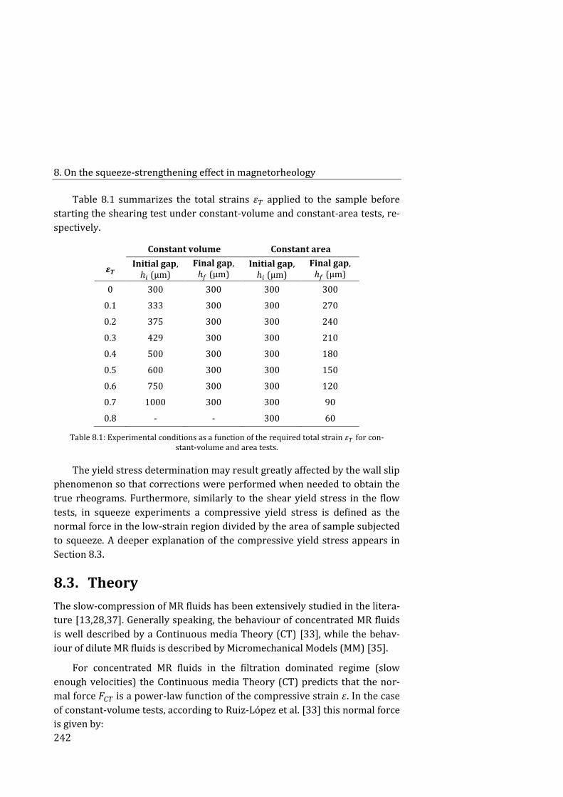
8. On the squeeze-strengthening effect in magnetorheology
242
Table 8.1 summarizes the total strains 휀𝑇 applied to the sample before
starting the shearing test under constant-volume and constant-area tests, re-
spectively.
Constant volume Constant area
𝜺𝑻 Initial gap,
ℎ𝑖 (μm) Final gap,
ℎ𝑓 (μm) Initial gap,
ℎ𝑖 (μm) Final gap,
ℎ𝑓 (μm)
0 300 300 300 300
0.1 333 300 300 270
0.2 375 300 300 240
0.3 429 300 300 210
0.4 500 300 300 180
0.5 600 300 300 150
0.6 750 300 300 120
0.7 1000 300 300 90
0.8 - - 300 60
Table 8.1: Experimental conditions as a function of the required total strain 휀𝑇 for con-stant-volume and area tests.
The yield stress determination may result greatly affected by the wall slip
phenomenon so that corrections were performed when needed to obtain the
true rheograms. Furthermore, similarly to the shear yield stress in the flow
tests, in squeeze experiments a compressive yield stress is defined as the
normal force in the low-strain region divided by the area of sample subjected
to squeeze. A deeper explanation of the compressive yield stress appears in
Section 8.3.
8.3. Theory
The slow-compression of MR fluids has been extensively studied in the litera-
ture [13,28,37]. Generally speaking, the behaviour of concentrated MR fluids
is well described by a Continuous media Theory (CT) [33], while the behav-
iour of dilute MR fluids is described by Micromechanical Models (MM) [35].
For concentrated MR fluids in the filtration dominated regime (slow
enough velocities) the Continuous media Theory (CT) predicts that the nor-
mal force 𝐹𝐶𝑇 is a power-law function of the compressive strain 휀. In the case
of constant-volume tests, according to Ruiz-López et al. [33] this normal force
is given by:
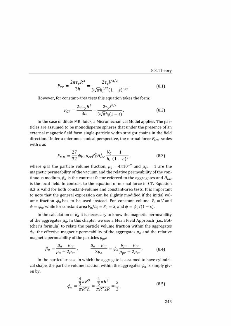
8.3. Theory
243
𝐹𝐶𝑇 =2𝜋𝜏𝑦𝑅3
3ℎ=
2𝜏𝑦𝑉3 2⁄
3√𝜋ℎ𝑖5 2⁄ (1 − 휀)5 2⁄
. (8.1)
However, for constant-area tests this equation takes the form:
𝐹𝐶𝑇 =2𝜋𝜏𝑦𝑅3
3ℎ=
2𝜏𝑦𝑆3/2
3√𝜋ℎ𝑖(1 − 휀) . (8.2)
In the case of dilute MR fluids, a Micromechanical Model applies. The par-
ticles are assumed to be monodisperse spheres that under the presence of an
external magnetic field form single-particle width straight chains in the field
direction. Under a micromechanical perspective, the normal force 𝐹𝑀𝑀 scales
with 휀 as
𝐹𝑀𝑀 =27
32𝜙𝜇0𝜇𝑐𝑟𝛽𝑎
2𝐻𝑙𝑜𝑐2
𝑉0
ℎ𝑖
1
(1 − 휀)2 , (8.3)
where 𝜙 is the particle volume fraction, 𝜇0 = 4𝜋10−7 and 𝜇𝑐𝑟 = 1 are the
magnetic permeability of the vacuum and the relative permeability of the con-
tinuous medium, 𝛽𝑎 is the contrast factor referred to the aggregates and 𝐻𝑙𝑜𝑐
is the local field. In contrast to the equation of normal force in CT, Equation
8.3 is valid for both constant-volume and constant-area tests. It is important
to note that the general expression can be slightly modified if the initial vol-
ume fraction 𝜙0 has to be used instead. For constant volume 𝑉0 = 𝑉 and
𝜙 = 𝜙0, while for constant area 𝑉0/ℎ𝑖 = 𝑆0 = 𝑆, and 𝜙 = 𝜙0/(1 − 휀).
In the calculation of 𝛽𝑎 it is necessary to know the magnetic permeability
of the aggregates 𝜇𝑎. In this chapter we use a Mean Field Approach (i.e., Böt-
tcher’s formula) to relate the particle volume fraction within the aggregates
𝜙𝑎, the effective magnetic permeability of the aggregates 𝜇𝑎 and the relative
magnetic permeability of the particles 𝜇𝑝𝑟:
𝛽𝑎 =𝜇𝑎 − 𝜇𝑐𝑟
𝜇𝑎 + 2𝜇𝑐𝑟 ,
𝜇𝑎 − 𝜇𝑐𝑟
3𝜇𝑎= 𝜙𝑎
𝜇𝑝𝑟 − 𝜇𝑐𝑟
𝜇𝑝𝑟 + 2𝜇𝑐𝑟 . (8.4)
In the particular case in which the aggregate is assumed to have cylindri-
cal shape, the particle volume fraction within the aggregates 𝜙𝑎 is simply giv-
en by:
𝜙𝑎 =
43 𝜋𝑅3
𝜋𝑅2ℎ=
43 𝜋𝑅3
𝜋𝑅22𝑅=
2
3 . (8.5)
8. On the squeeze-strengthening effect in magnetorheology
244
The relative magnetic permeability of the particles 𝜇𝑝𝑟 is calculated here
using the Fröhlich-Kennelly equation [38]:
𝜇𝑝𝑟(𝐻0) = 1 +(𝜇0 − 1)
𝑀𝑠
𝐻0
(𝜇0 − 1) +𝑀𝑠
𝐻0 . (8.6)
The relative initial magnetic permeability and the saturation magnetiza-
tion were taken as 𝜇0 = 40 and 𝑀𝑠 = 1550 kA · m−1, respectively [39]. The
relative magnetic permeability of the particles at the external magnetic field
used in the experiments was 𝜇𝑝𝑟 = 9.97. By solving the Böttcher’s equation,
𝜇𝑎 = 5.84, and 𝛽𝑎 = 0.617.
At this stage it is very important to note that Equation 8.3 is valid for both
constant-volume and constant-area operation modes. In both CT and MM
models, the normal force can be normalized by a pre-factor 𝐴, that corre-
sponds to the low-strain normal force plateau: 𝐹 = 𝐴 (1 − 휀)𝐵⁄ . In summary,
while for CT the normal force scales with (1 − 휀)−5/2 , in MM it scales accord-
ing to (1 − 휀)−2. In the following section we will compare experimental data
with MM predictions.
8.4. Squeeze simulations
Similarly to the experimental case, squeeze simulations were performed in
constant-area and constant-volume modes. Particle-level simulations were
employed and Langevin equation (Equation 3.16) was solved at each time
step. It is the equation of motion that better describes the interactions be-
tween Brownian particles, as it contains terms accounting for the determinis-
tic motion of the particles but also additional stochastic forces. The simulation
code contains three steps that are equivalent to the experimental protocol:
particle structuration, squeeze and shear, while considering a constant mag-
netic field of 𝐻0 = 177 kA · m−1 during the whole protocol.
Brownian dynamics simulations were carried out to simulate systems of
1000 monodisperse spherical magnetic particles. The volume fraction was
varied among 𝜙 = 0.05 and 0.30. We used periodic boundary conditions in 𝑥
and 𝑦 directions, and two initial gaps ℎ𝑖 were studied, namely 20 and 30 times
the mean diameter 𝜎𝑚 (i.e., ℎ𝑖 = 20 𝜎𝑚, 30 𝜎𝑚), which is employed as a length
scale. So that, depending on the initial gap and the volume fraction, the other
two dimensions of the simulation box can be easily determined. Particles are
8.4. Squeeze simulations
245
randomly distributed in the simulation box and overlap is forbidden. The
magnetic dipoles of the particles are supposed to be equal at the onset of the
simulation and oriented with the magnetic field, it is, in 𝑧 axis.
Local magnetic field 𝑯𝒍𝒐𝒄𝒊 is considered in the calculation of the magnetic
force between pairs of particles (see Equations from 8.7 to 8.10). In this
sense, for a given particle its magnetic force is due both to the external mag-
netic field 𝑯𝟎 and the rest of dipolar contributions from other particles 𝑯𝒎𝒋
that surround it at distances lower than a stablished cut-off.
𝒎𝒊 =𝜋
2𝛽𝑯𝒍𝒐𝒄𝒊
𝜎𝑖3 , (8.7)
𝑯𝒍𝒐𝒄,𝒊 = 𝑯𝟎 + ∑ 𝑯𝒎𝒋
𝑁𝑝𝑐
𝑗≠𝑖
, (8.8)
𝑯𝒎𝒋=
3(𝒎𝒋 · �̂�)�̂� − 𝒎𝒋
𝑟𝑖𝑗3 , (8.9)
𝑭𝒊𝒋𝒎 =
3
4
𝜇0𝜇𝑐𝑟
𝜋[(𝒎𝒊 · 𝒎𝒋)𝒓𝒊𝒋 + (𝒎𝒊 · 𝒓𝒊𝒋)𝒎𝒋 + (𝒎𝒋 · 𝒓𝒊𝒋)𝒎𝒊
𝑟𝑖𝑗5 −
−5(𝒎𝒊 · 𝒓𝒊𝒋)(𝒎𝒋 · 𝒓𝒊𝒋)𝒓𝒊𝒋
𝑟𝑖𝑗7 ]
(8.10)
Apart from magnetic interactions, Stoke’s drag (Equation 8.11) and
Brownian forces (Equation 8.12) are taken into account, as well as an expo-
nential repulsive force that decays with particle separation (Equation 8.13) as
expressed below:
𝑭𝒊𝑺 = −𝜉𝑖 (
𝑑𝒓𝒊
𝑑𝑡− 𝒖𝒊
∞) = −3𝜋휂𝜎𝑖𝒗𝒊 , (8.11)
𝒇𝑩∗ ∝ √
𝑘𝐵𝑇
𝜎𝑚𝐹0
√𝜎𝑖
∗
∆𝑡∗ , (8.12)
𝑭𝒊𝒋𝒓 = 𝐹0𝑒−𝑘(𝑟𝑖𝑗−(𝜎𝑖+𝜎𝑗)/2)�̂�𝒊𝒋 , (8.13)
where 𝜉𝑖 = 3𝜋휂𝜎𝑖 is the friction coefficient of particle 𝑖, 휂 is the fluid viscosity
and 𝜎𝑖 is the particle diameter; 𝑘𝐵 = 1.381 · 10−23 J · K−1 is the Boltzmann
constant and 𝑇 the absolute temperature expressed in kelvin; 𝐹0 is the force
8. On the squeeze-strengthening effect in magnetorheology
246
scale, 𝑘 = 100 and 𝑟𝑖𝑗is the center-to-center distance between particles 𝑖 and
𝑗.
Langevin equation used within the simulation code neglects inertia so
that it takes the form of
𝜉𝑖
𝑑𝒓𝒊
𝑑𝑡= 𝜉𝑖𝒖𝒊
∞ + 𝑭𝒊𝒎 + 𝑭𝒊
𝒓 + 𝑭𝒃 . (8.14)
In order to solve Equation 8.14 it is convenient to make it dimensionless
by means of scaling parameters showed in Table 3.5.
The inertialess Langevin equation (Equation 8.14) is solved at each time
step and the new particle positions are considered in the next time step. In
the structuration step the main contribution to the particle movements comes
from magnetic interactions. The normalized time for structuration is suffi-
cient to obtain steady states in the magnetic energy, normal stress, normal
force and number of neighbours. After that, the particle configuration is sub-
jected to the squeeze step, in which the gap is steadily forced to diminish at a
given velocity, and so the height of the simulation box. The time during which
the gap diminishes depends on the required level of deformation. In constant-
volume simulations it provokes an enlargement in the other dimensions of
the simulation box, so that particles have to fit in a modified simulation box
that keeps the initial volume and, as a consequence, the volume fraction does
not vary. On the contrary, in constant-area simulations the gap is diminished,
while the other two dimensions preserve their initial lengths so that the simu-
lation box is smaller. As it occurs in the experimental case, particles are con-
fined in the area subjected to the magnetic field and cannot abandon the new
simulation box, so that the volume fraction increases with 휀 in constant-area
conditions. Once a given deformation is achieved, the shear flow is activated
at constant shear rates. The effect of the compression of the magnetic struc-
tures in the static yield stress under shear is compared for both types of simu-
lations.
8.5. Results and Discussion
8.5.1. Squeeze flow behaviour of MR fluids
The compression curves for constant-volume tests (𝑉 = 110 μL) are shown in
Figure 8.9-a. Accordingly with the equation of normal force in micromechani-
cal models (Equation 8.3), for a given 휀𝑇 , the experimental normal force 𝐹𝑁
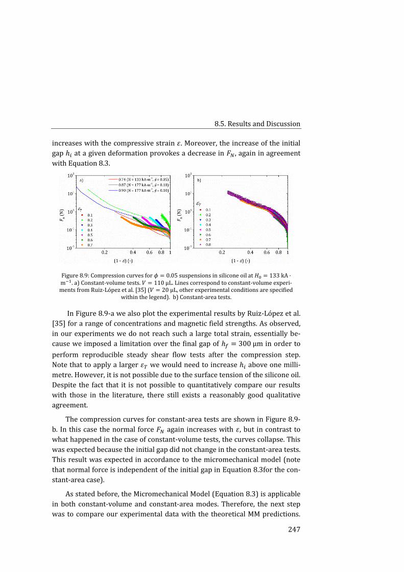
8.5. Results and Discussion
247
increases with the compressive strain 휀. Moreover, the increase of the initial
gap ℎ𝑖 at a given deformation provokes a decrease in 𝐹𝑁, again in agreement
with Equation 8.3.
Figure 8.9: Compression curves for 𝜙 = 0.05 suspensions in silicone oil at 𝐻0 = 133 kA ·m−1. a) Constant-volume tests. 𝑉 = 110 μL. Lines correspond to constant-volume experi-ments from Ruiz-López et al. [35] (𝑉 = 20 μL, other experimental conditions are specified
within the legend). b) Constant-area tests.
In Figure 8.9-a we also plot the experimental results by Ruiz-López et al.
[35] for a range of concentrations and magnetic field strengths. As observed,
in our experiments we do not reach such a large total strain, essentially be-
cause we imposed a limitation over the final gap of ℎ𝑓 = 300 µm in order to
perform reproducible steady shear flow tests after the compression step.
Note that to apply a larger 휀𝑇 we would need to increase ℎ𝑖 above one milli-
metre. However, it is not possible due to the surface tension of the silicone oil.
Despite the fact that it is not possible to quantitatively compare our results
with those in the literature, there still exists a reasonably good qualitative
agreement.
The compression curves for constant-area tests are shown in Figure 8.9-
b. In this case the normal force 𝐹𝑁 again increases with 휀, but in contrast to
what happened in the case of constant-volume tests, the curves collapse. This
was expected because the initial gap did not change in the constant-area tests.
This result was expected in accordance to the micromechanical model (note
that normal force is independent of the initial gap in Equation 8.3for the con-
stant-area case).
As stated before, the Micromechanical Model (Equation 8.3) is applicable
in both constant-volume and constant-area modes. Therefore, the next step
was to compare our experimental data with the theoretical MM predictions.
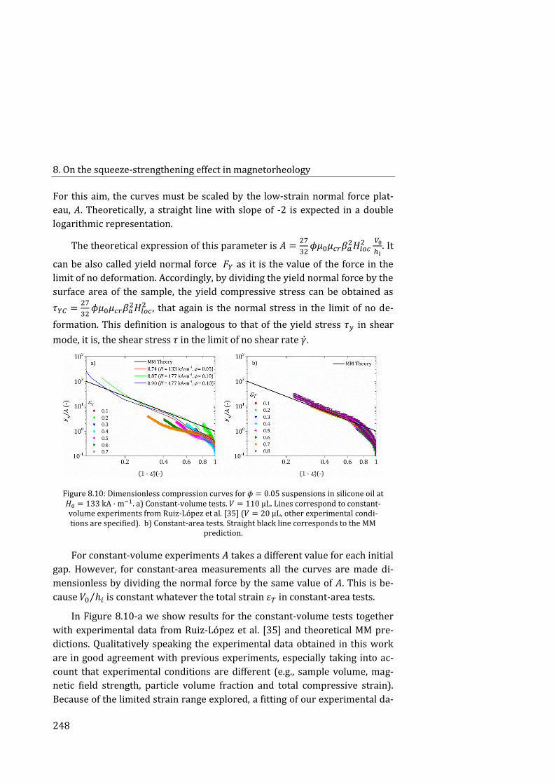
8. On the squeeze-strengthening effect in magnetorheology
248
For this aim, the curves must be scaled by the low-strain normal force plat-
eau, 𝐴. Theoretically, a straight line with slope of -2 is expected in a double
logarithmic representation.
The theoretical expression of this parameter is 𝐴 =27
32𝜙𝜇0𝜇𝑐𝑟𝛽𝑎
2𝐻𝑙𝑜𝑐2 𝑉0
ℎ𝑖. It
can be also called yield normal force 𝐹𝑌 as it is the value of the force in the
limit of no deformation. Accordingly, by dividing the yield normal force by the
surface area of the sample, the yield compressive stress can be obtained as
𝜏𝑌𝐶 =27
32𝜙𝜇0𝜇𝑐𝑟𝛽𝑎
2𝐻𝑙𝑜𝑐2 , that again is the normal stress in the limit of no de-
formation. This definition is analogous to that of the yield stress 𝜏𝑦 in shear
mode, it is, the shear stress 𝜏 in the limit of no shear rate �̇�.
Figure 8.10: Dimensionless compression curves for 𝜙 = 0.05 suspensions in silicone oil at 𝐻0 = 133 kA · m−1. a) Constant-volume tests. 𝑉 = 110 μL. Lines correspond to constant-volume experiments from Ruiz-López et al. [35] (𝑉 = 20 μL, other experimental condi-tions are specified). b) Constant-area tests. Straight black line corresponds to the MM
prediction.
For constant-volume experiments 𝐴 takes a different value for each initial
gap. However, for constant-area measurements all the curves are made di-
mensionless by dividing the normal force by the same value of 𝐴. This is be-
cause 𝑉0 ℎ𝑖⁄ is constant whatever the total strain 휀𝑇 in constant-area tests.
In Figure 8.10-a we show results for the constant-volume tests together
with experimental data from Ruiz-López et al. [35] and theoretical MM pre-
dictions. Qualitatively speaking the experimental data obtained in this work
are in good agreement with previous experiments, especially taking into ac-
count that experimental conditions are different (e.g., sample volume, mag-
netic field strength, particle volume fraction and total compressive strain).
Because of the limited strain range explored, a fitting of our experimental da-
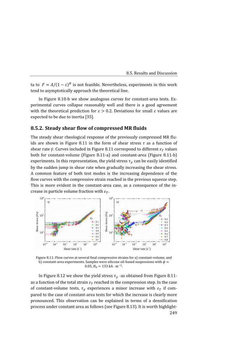
8.5. Results and Discussion
249
ta to 𝐹 = 𝐴/(1 − 휀)𝐵 is not feasible. Nevertheless, experiments in this work
tend to asymptotically approach the theoretical line.
In Figure 8.10-b we show analogous curves for constant-area tests. Ex-
perimental curves collapse reasonably well and there is a good agreement
with the theoretical prediction for 휀 > 0.2. Deviations for small 휀 values are
expected to be due to inertia [35].
8.5.2. Steady shear flow of compressed MR fluids
The steady shear rheological response of the previously compressed MR flu-
ids are shown in Figure 8.11 in the form of shear stress 𝜏 as a function of
shear rate �̇�. Curves included in Figure 8.11 correspond to different 휀𝑇 values
both for constant-volume (Figure 8.11-a) and constant-area (Figure 8.11-b)
experiments. In this representation, the yield stress 𝜏𝑦 can be easily identified
by the sudden jump in shear rate when gradually increasing the shear stress.
A common feature of both test modes is the increasing dependence of the
flow curves with the compressive strain reached in the previous squeeze step.
This is more evident in the constant-area case, as a consequence of the in-
crease in particle volume fraction with 휀𝑇 .
Figure 8.11: Flow curves at several final compressive strains for a) constant-volume, and b) constant-area experiments. Samples were silicone oil-based suspensions with 𝜙 =
0.05, 𝐻0 = 133 kA · m−1.
In Figure 8.12 we show the yield stress 𝜏𝑦 -as obtained from Figure 8.11-
as a function of the total strain 휀𝑇 reached in the compression step. In the case
of constant-volume tests, 𝜏𝑦 experiences a minor increase with 휀𝑇 if com-
pared to the case of constant-area tests for which the increase is clearly more
pronounced. This observation can be explained in terms of a densification
process under constant area as follows (see Figure 8.13). It is worth highlight-
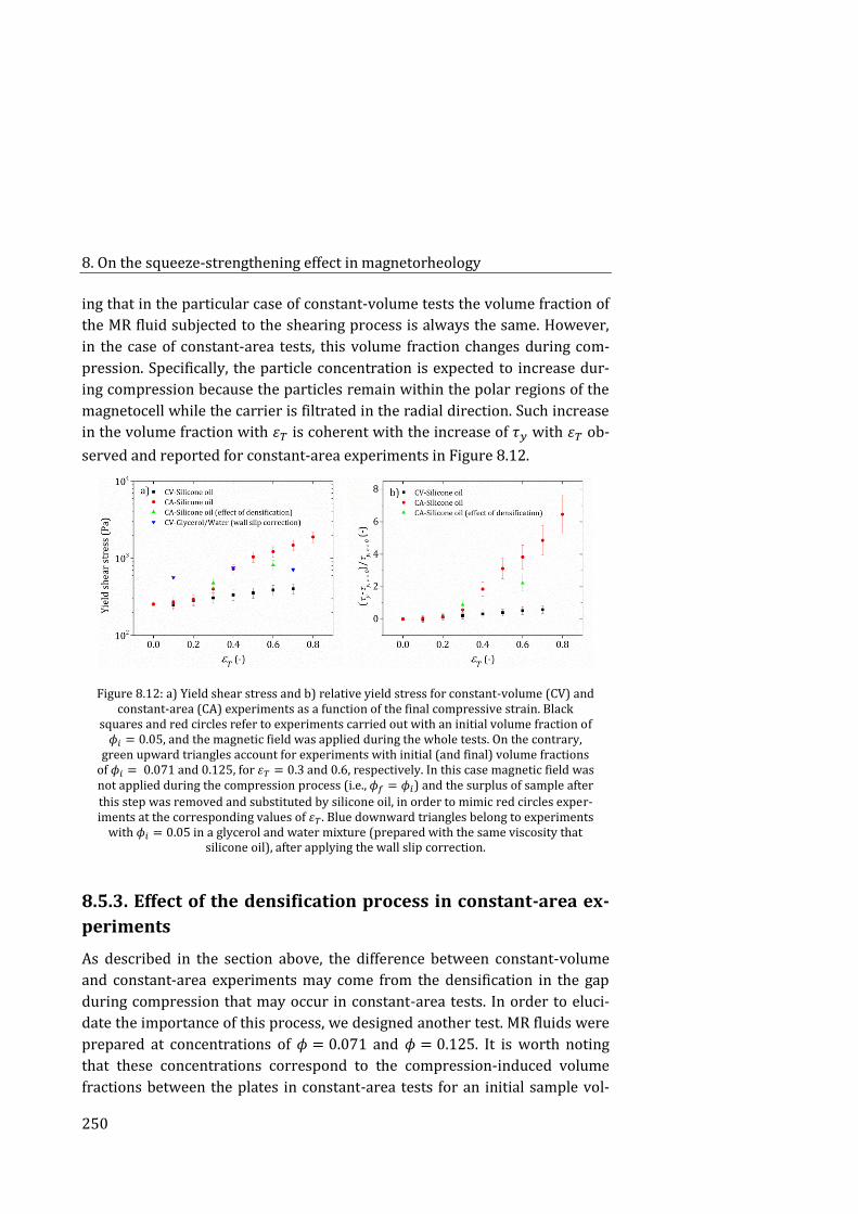
8. On the squeeze-strengthening effect in magnetorheology
250
ing that in the particular case of constant-volume tests the volume fraction of
the MR fluid subjected to the shearing process is always the same. However,
in the case of constant-area tests, this volume fraction changes during com-
pression. Specifically, the particle concentration is expected to increase dur-
ing compression because the particles remain within the polar regions of the
magnetocell while the carrier is filtrated in the radial direction. Such increase
in the volume fraction with 휀𝑇 is coherent with the increase of 𝜏𝑦 with 휀𝑇 ob-
served and reported for constant-area experiments in Figure 8.12.
Figure 8.12: a) Yield shear stress and b) relative yield stress for constant-volume (CV) and constant-area (CA) experiments as a function of the final compressive strain. Black
squares and red circles refer to experiments carried out with an initial volume fraction of 𝜙𝑖 = 0.05, and the magnetic field was applied during the whole tests. On the contrary,
green upward triangles account for experiments with initial (and final) volume fractions of 𝜙𝑖 = 0.071 and 0.125, for 휀𝑇 = 0.3 and 0.6, respectively. In this case magnetic field was not applied during the compression process (i.e., 𝜙𝑓 = 𝜙𝑖) and the surplus of sample after
this step was removed and substituted by silicone oil, in order to mimic red circles exper-iments at the corresponding values of 휀𝑇. Blue downward triangles belong to experiments
with 𝜙𝑖 = 0.05 in a glycerol and water mixture (prepared with the same viscosity that silicone oil), after applying the wall slip correction.
8.5.3. Effect of the densification process in constant-area ex-
periments
As described in the section above, the difference between constant-volume
and constant-area experiments may come from the densification in the gap
during compression that may occur in constant-area tests. In order to eluci-
date the importance of this process, we designed another test. MR fluids were
prepared at concentrations of 𝜙 = 0.071 and 𝜙 = 0.125. It is worth noting
that these concentrations correspond to the compression-induced volume
fractions between the plates in constant-area tests for an initial sample vol-
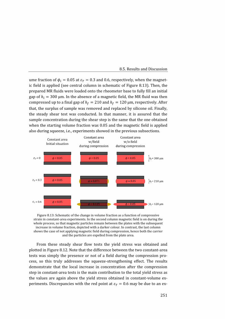
8.5. Results and Discussion
251
ume fraction of 𝜙𝑖 = 0.05 at 휀𝑇 = 0.3 and 0.6, respectively, when the magnet-
ic field is applied (see central column in schematic of Figure 8.13). Then, the
prepared MR fluids were loaded onto the rheometer base to fully fill an initial
gap of ℎ𝑖 = 300 µm. In the absence of a magnetic field, the MR fluid was then
compressed up to a final gap of ℎ𝑓 = 210 and ℎ𝑓 = 120 µm, respectively. After
that, the surplus of sample was removed and replaced by silicone oil. Finally,
the steady shear test was conducted. In that manner, it is assured that the
sample concentration during the shear step is the same that the one obtained
when the starting volume fraction was 0.05 and the magnetic field is applied
also during squeeze, i.e., experiments showed in the previous subsections.
Figure 8.13: Schematic of the change in volume fraction as a function of compressive strain in constant-area experiments. In the second column magnetic field is on during the whole process, so that magnetic particles remain between the plates with the subsequent
increase in volume fraction, depicted with a darker colour. In contrast, the last column shows the case of not applying magnetic field during compression, hence both the carrier
and the particles are expelled from the plate area.
From these steady shear flow tests the yield stress was obtained and
plotted in Figure 8.12. Note that the difference between the two constant-area
tests was simply the presence or not of a field during the compression pro-
cess, so this truly addresses the squeeze-strengthening effect. The results
demonstrate that the local increase in concentration after the compression
step in constant-area tests is the main contribution to the total yield stress as
the values are again above the yield stress obtained in constant-volume ex-
periments. Discrepancies with the red point at 휀𝑇 = 0.6 may be due to an ex-
8. On the squeeze-strengthening effect in magnetorheology
252
cessive removal of sample at the end of the squeeze step, that would mean a
lower magnetic particle concentration and would explain the lower 𝜏𝑦.
8.5.4. Influence of the carrier fluid in the compression
behaviour of MR fluids in constant-volume tests
As observed in Figure 8.10-a, corresponding to constant-volume experiments
with silicone oil, there is a shoulder in most of the curves at small defor-
mations, which could be associated to surface tension effects, wall slip, wetta-
bility or sedimentation. In order to evaluate the importance of the carrier flu-
id employed in the compression process we decided to prepare a new set of
MR fluids based on glycerol.
In Figure 8.14-a we show the normalized normal force as a function of the
compressive strain in constant-volume essays. All the curves are above the
theoretical MM prediction. This is in contrast to the case of silicone oil sus-
pensions and can be related to higher surface tension in glycerol. The curve
corresponding to the highest compressive strains (i.e., the largest initial gap)
is closer to the theoretical line, maybe because edge effects are reduced in
comparison with lower gaps. In Figure 8.14-b we show the rheograms of the
compressed glycerol-based MR fluids. As observed, there is a clear shoulder
evidencing wall slip. In this case the breaking process is smoother if com-
pared to silicone oil-based MR fluids.
In order to give a better insight we decided to prepare MR fluids in glyc-
erol (87 % w/w, Scharlau)-water mixtures (80.59:19.41 % w:w) with exactly
the same viscosity as the silicone oil employed before (19 mPa). By doing
this, the influence of viscosity can be discarded. In Figure 8.15-a we present
the normal force curves for three different total compressive strains (휀𝑇 =
0.1, 0.4 and 0.7) at four different final gaps (ℎ𝑓 = 0.1, 0.2, 0.3 and 0.4 mm). In
this sense, the volume of sample was varied proportionally to the final gap in
order to the sample completely fill the volume between plates at the begin-
ning of the shear step. Four different gaps where tested in order to correct the
wall slip in the steady shear process [40]. As expected, there is not a differ-
ence for the ℎ𝑓 studied. It can be explained from Equation 8.3 as the volume of
sample is proportional to the final gap, so that at a given 휀𝑇 the ratio 𝑉0/ℎ𝑓 is
the same for each measurement condition and the normal force does not
change. For the same reason, higher final compressive strains result in lower
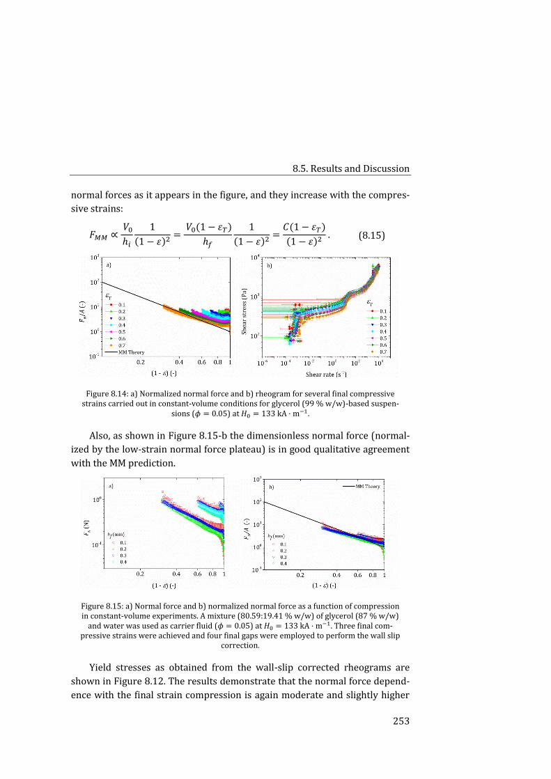
8.5. Results and Discussion
253
normal forces as it appears in the figure, and they increase with the compres-
sive strains:
𝐹𝑀𝑀 ∝ 𝑉0
ℎ𝑖
1
(1 − 휀)2=
𝑉0(1 − 휀𝑇)
ℎ𝑓
1
(1 − 휀)2=
𝐶(1 − 휀𝑇)
(1 − 휀)2 . (8.15)
Figure 8.14: a) Normalized normal force and b) rheogram for several final compressive strains carried out in constant-volume conditions for glycerol (99 % w/w)-based suspen-
sions (𝜙 = 0.05) at 𝐻0 = 133 kA · m−1.
Also, as shown in Figure 8.15-b the dimensionless normal force (normal-
ized by the low-strain normal force plateau) is in good qualitative agreement
with the MM prediction.
Figure 8.15: a) Normal force and b) normalized normal force as a function of compression in constant-volume experiments. A mixture (80.59:19.41 % w/w) of glycerol (87 % w/w)
and water was used as carrier fluid (𝜙 = 0.05) at 𝐻0 = 133 kA · m−1. Three final com-pressive strains were achieved and four final gaps were employed to perform the wall slip
correction.
Yield stresses as obtained from the wall-slip corrected rheograms are
shown in Figure 8.12. The results demonstrate that the normal force depend-
ence with the final strain compression is again moderate and slightly higher
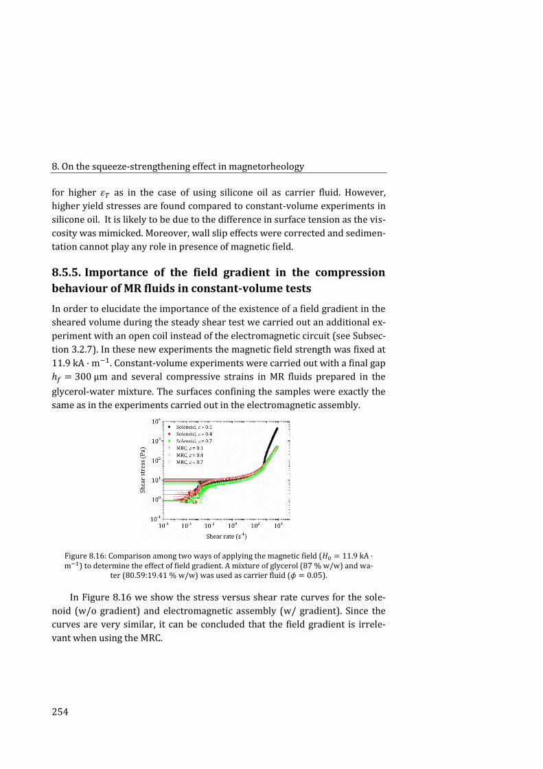
8. On the squeeze-strengthening effect in magnetorheology
254
for higher 휀𝑇 as in the case of using silicone oil as carrier fluid. However,
higher yield stresses are found compared to constant-volume experiments in
silicone oil. It is likely to be due to the difference in surface tension as the vis-
cosity was mimicked. Moreover, wall slip effects were corrected and sedimen-
tation cannot play any role in presence of magnetic field.
8.5.5. Importance of the field gradient in the compression
behaviour of MR fluids in constant-volume tests
In order to elucidate the importance of the existence of a field gradient in the
sheared volume during the steady shear test we carried out an additional ex-
periment with an open coil instead of the electromagnetic circuit (see Subsec-
tion 3.2.7). In these new experiments the magnetic field strength was fixed at
11.9 kA · m−1. Constant-volume experiments were carried out with a final gap
ℎ𝑓 = 300 µm and several compressive strains in MR fluids prepared in the
glycerol-water mixture. The surfaces confining the samples were exactly the
same as in the experiments carried out in the electromagnetic assembly.
Figure 8.16: Comparison among two ways of applying the magnetic field (𝐻0 = 11.9 kA ·m−1) to determine the effect of field gradient. A mixture of glycerol (87 % w/w) and wa-
ter (80.59:19.41 % w/w) was used as carrier fluid (𝜙 = 0.05).
In Figure 8.16 we show the stress versus shear rate curves for the sole-
noid (w/o gradient) and electromagnetic assembly (w/ gradient). Since the
curves are very similar, it can be concluded that the field gradient is irrele-
vant when using the MRC.
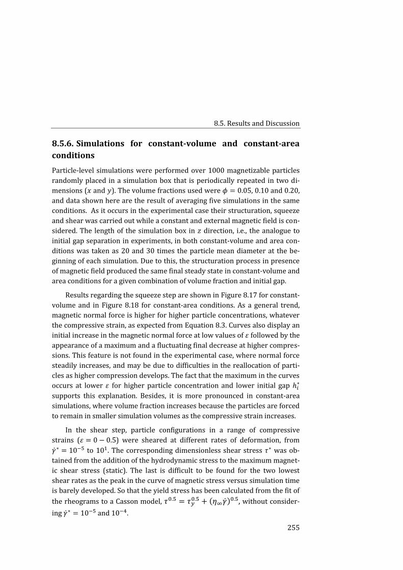
8.5. Results and Discussion
255
8.5.6. Simulations for constant-volume and constant-area
conditions
Particle-level simulations were performed over 1000 magnetizable particles
randomly placed in a simulation box that is periodically repeated in two di-
mensions (𝑥 and 𝑦). The volume fractions used were 𝜙 = 0.05, 0.10 and 0.20,
and data shown here are the result of averaging five simulations in the same
conditions. As it occurs in the experimental case their structuration, squeeze
and shear was carried out while a constant and external magnetic field is con-
sidered. The length of the simulation box in 𝑧 direction, i.e., the analogue to
initial gap separation in experiments, in both constant-volume and area con-
ditions was taken as 20 and 30 times the particle mean diameter at the be-
ginning of each simulation. Due to this, the structuration process in presence
of magnetic field produced the same final steady state in constant-volume and
area conditions for a given combination of volume fraction and initial gap.
Results regarding the squeeze step are shown in Figure 8.17 for constant-
volume and in Figure 8.18 for constant-area conditions. As a general trend,
magnetic normal force is higher for higher particle concentrations, whatever
the compressive strain, as expected from Equation 8.3. Curves also display an
initial increase in the magnetic normal force at low values of 휀 followed by the
appearance of a maximum and a fluctuating final decrease at higher compres-
sions. This feature is not found in the experimental case, where normal force
steadily increases, and may be due to difficulties in the reallocation of parti-
cles as higher compression develops. The fact that the maximum in the curves
occurs at lower 휀 for higher particle concentration and lower initial gap ℎ𝑖∗
supports this explanation. Besides, it is more pronounced in constant-area
simulations, where volume fraction increases because the particles are forced
to remain in smaller simulation volumes as the compressive strain increases.
In the shear step, particle configurations in a range of compressive
strains (휀 = 0 − 0.5) were sheared at different rates of deformation, from
�̇�∗ = 10−5 to 101. The corresponding dimensionless shear stress 𝜏∗ was ob-
tained from the addition of the hydrodynamic stress to the maximum magnet-
ic shear stress (static). The last is difficult to be found for the two lowest
shear rates as the peak in the curve of magnetic stress versus simulation time
is barely developed. So that the yield stress has been calculated from the fit of
the rheograms to a Casson model, 𝜏0.5 = 𝜏𝑦0.5 + (휂∞�̇�)0.5, without consider-
ing �̇�∗ = 10−5 and 10−4.
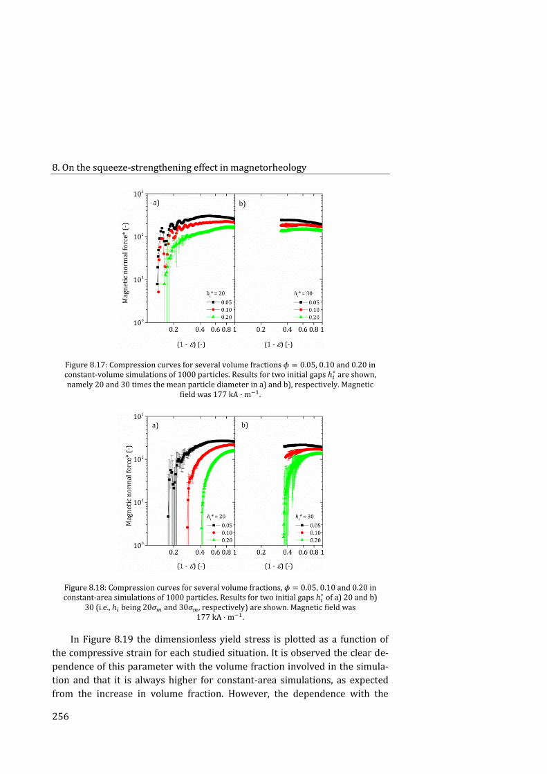
8. On the squeeze-strengthening effect in magnetorheology
256
Figure 8.17: Compression curves for several volume fractions 𝜙 = 0.05, 0.10 and 0.20 in constant-volume simulations of 1000 particles. Results for two initial gaps ℎ𝑖
∗ are shown, namely 20 and 30 times the mean particle diameter in a) and b), respectively. Magnetic
field was 177 kA · m−1.
Figure 8.18: Compression curves for several volume fractions, 𝜙 = 0.05, 0.10 and 0.20 in constant-area simulations of 1000 particles. Results for two initial gaps ℎ𝑖
∗ of a) 20 and b) 30 (i.e., ℎ𝑖 being 20𝜎𝑚 and 30𝜎𝑚, respectively) are shown. Magnetic field was
177 kA · m−1.
In Figure 8.19 the dimensionless yield stress is plotted as a function of
the compressive strain for each studied situation. It is observed the clear de-
pendence of this parameter with the volume fraction involved in the simula-
tion and that it is always higher for constant-area simulations, as expected
from the increase in volume fraction. However, the dependence with the
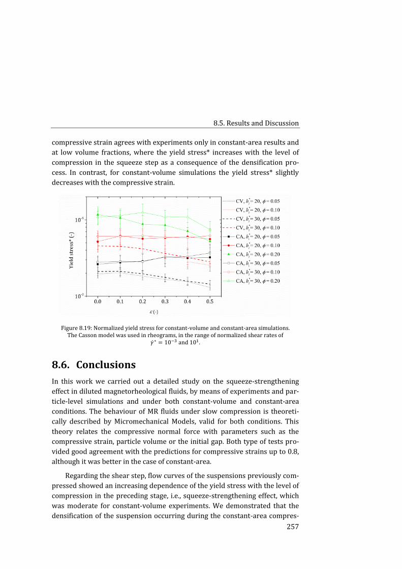
8.5. Results and Discussion
257
compressive strain agrees with experiments only in constant-area results and
at low volume fractions, where the yield stress* increases with the level of
compression in the squeeze step as a consequence of the densification pro-
cess. In contrast, for constant-volume simulations the yield stress* slightly
decreases with the compressive strain.
Figure 8.19: Normalized yield stress for constant-volume and constant-area simulations. The Casson model was used in rheograms, in the range of normalized shear rates of
�̇�∗ = 10−3 and 101.
8.6. Conclusions
In this work we carried out a detailed study on the squeeze-strengthening
effect in diluted magnetorheological fluids, by means of experiments and par-
ticle-level simulations and under both constant-volume and constant-area
conditions. The behaviour of MR fluids under slow compression is theoreti-
cally described by Micromechanical Models, valid for both conditions. This
theory relates the compressive normal force with parameters such as the
compressive strain, particle volume or the initial gap. Both type of tests pro-
vided good agreement with the predictions for compressive strains up to 0.8,
although it was better in the case of constant-area.
Regarding the shear step, flow curves of the suspensions previously com-
pressed showed an increasing dependence of the yield stress with the level of
compression in the preceding stage, i.e., squeeze-strengthening effect, which
was moderate for constant-volume experiments. We demonstrated that the
densification of the suspension occurring during the constant-area compres-
8. On the squeeze-strengthening effect in magnetorheology
258
sion is responsible to a large extent of the higher values of yield stress com-
pared to constant-volume tests. Moreover constant-volume squeeze experi-
ments were carried out in silicone oil and glycerol/water mixtures with the
same particle loading. In this sense, we observed for each compressive strain
an increasing effect in the yield stress that may be uniquely due to the surface
tension in the yield stress, as the viscosities were matched. Additionally, we
compared experiments carried out using a coil and a magnetorheological cell
and evidenced an insignificant effect of the field gradient.
Particle-level simulations mimicked the experimental stages, i.e., structu-
ration at rest, compression and shear, and the effect of volume fraction, total
compressive strains up to 0.5, and initial gap under constant-volume and con-
stant-area conditions were studied. In these simulations we found a depend-
ence of yield stress with the compressive strain, and although both positive
and negative tendencies are shown, yield stress values from constant-area
simulations are always above those from the constant-volume case as a con-
sequence of the densification process, in agreement with experiments.
8.7. References
[1] Rankin P J, Ginder J M and Klingenberg D J 1998 Electro- and magne-
to-rheology Curr. Opin. Colloid Interface Sci. 3 373–381
[2] Klingenberg D J 2001 Magnetorheology: Applications and challenges
AIChE J. 47 246–249
[3] Ginder J M 2003 Rheology Controlled by Magnetic Fields Digital Ency-
clopedia of Applied Physics ed Wiley-VCH Verlag GmbH & Co. KGaA (Wein-
heim, Germany: Wiley-VCH Verlag GmbH & Co. KGaA)
[4] de Vicente J, Klingenberg D J and Hidalgo-Álvarez R 2011 Magne-
torheological fluids: a review Soft Matter 7 3701
[5] Carlson J D and Jolly M R 2000 MR fluid, foam and elastomer devices
Mechatronics 10 555–569
[6] Olabi A G and Grunwald A 2007 Design and application of magneto-
rheological fluid Mater. Des. 28 2658–2664
[7] Kulkarni P, Ciocanel C, Vieira S L and Naganathan N 2003 Study of the
Behavior of MR Fluids in Squeeze, Torsional and Valve Modes J. Intell. Mater.
Syst. Struct. 14 99–104
8.7. References
259
[8] Wang X and Gordaninejad F 2006 Study of magnetorheological fluids
at high shear rates Rheol. Acta 45 899–908
[9] Rodríguez-Arco L, Kuzhir P, López-López M T, Bossis G and Durán J D
G 2013 Instabilities of a pressure-driven flow of magnetorheological fluids J.
Rheol. 57 1121–46
[10] de Vicente J, López-López M T, Durán J D G and González-Caballero F
2004 Shear flow behavior of confined magnetorheological fluids at low mag-
netic field strengths Rheol. Acta 44 94–103
[11] Ramos J, Klingenberg D J, Hidalgo-Alvarez R and Vicente J de 2011
Steady shear magnetorheology of inverse ferrofluids J. Rheol. 55 127–152
[12] Zhang X Z, Gong X L, Zhang P Q and Wang Q M 2004 Study on the
mechanism of the squeeze-strengthen effect in magnetorheological fluids J.
Appl. Phys. 96 2359–2364
[13] de Vicente J, Ruiz-lópez J A, Andablo-reyes E, Segovia-gutiérrez J P
and Hidalgo-alvarez R 2011 Squeeze flow magnetorheology J. Rheol. 55 753–
79
[14] See H, Mackenzie S and Chua B T 2006 Effect of compression on the
response of a magneto-rheological suspension Korea-Aust. Rheol. J. 18 121–
126
[15] Bigué J-P L, Charron F and Plante J-S 2015 Understanding the super-
strong behavior of magnetorheological fluid in simultaneous squeeze-shear
with the Péclet number J. Intell. Mater. Syst. Struct. 26 1844–1855
[16] Becnel A C, Sherman S G, Hu W and Wereley N M 2015 Squeeze
strengthening of magnetorheological fluids using mixed mode operation J.
Appl. Phys. 117 17C708
[17] Vieira S L, Ciocanel C, Kulkarni P, Agrawal A and Naganathan N 2003
Behaviour of MR fluids in squeeze mode Int. J. Veh. Des. 33 36
[18] Dienes G J and Klemm H F 1946 Theory and Application of the Paral-
lel Plate Plastometer J. Appl. Phys. 17 458–71
[19] Covey G H and Stanmore B R 1981 Use of the parallel-plate plastome-
ter for the characterisation of viscous fluids with a yield stress J. Non-Newton.
Fluid Mech. 8 249–260
8. On the squeeze-strengthening effect in magnetorheology
260
[20] Williams E W, Rigby S G, Sproston J L and Stanway R 1993 Electro-
rheological fluids applied to an automotive engine mount J. Non-Newton. Fluid
Mech. 47 221–38
[21] Monkman G J 1995 The electrorheological effect under compressive
stress J. Phys. Appl. Phys. 28 588–93
[22] Vieira S L and de Arruda A C F 1998 Electrorheological Fluids Re-
sponse under Mechanical Testing J. Intell. Mater. Syst. Struct. 9 44–52
[23] Chu S-H, Lee S J and Ahn K H 2000 An experimental study on the
squeezing flow of electrorheological suspensions J. Rheol. 44 105–120
[24] Meng Y and Filisko F E 2005 Unidirectional compression of electro-
rheological fluids in electric fields J. Appl. Phys. 98 074901
[25] McIntyre E C and Filisko F E 2007 Squeeze Flow of Electrorheological
Fluids Under Constant Volume J. Intell. Mater. Syst. Struct. 18 1217–1220
[26] Guo C, Gong X, Xuan S, Yan Q and Ruan X 2013 Squeeze behavior of
magnetorheological fluids under constant volume and uniform magnetic field
Smart Mater. Struct. 22 045020
[27] Yangguang Xu, Xinglong Gong, Taixiang Liu and Shouhu Xuan 2014
Squeeze flow behaviors of magnetorheological plastomers under constant
volume J. Rheol. 58 659–79
[28] Tang X, Zhang X, Tao R and Rong Y 2000 Structure-enhanced Yield
Stress of Magnetorheological Fluids J. Appl. Phys. 87 2634
[29] Tang X, Zhang X and Tao R 2001 Enhance the Yield Shear Stress of
Magnetorheological Fluids Int. J. Mod. Phys. B 15 549–56
[30] Hegger C and Maas J 2016 Investigation of the squeeze strengthening
effect in shear mode J. Intell. Mater. Syst. Struct. 27 1895–1907
[31] Ghaffari A, Hashemabadi S H and Ashtiani M 2014 A review on the
simulation and modeling of magnetorheological fluids J. Intell. Mater. Syst.
Struct. 26 881–904
[32] Farjoud A, Ahmadian M, Mahmoodi N, Zhang X and Craft M 2011 Non-
linear modeling and testing of magneto-rheological fluids in low shear rate
squeezing flows Smart Mater. Struct. 20 085013
8.7. References
261
[33] Ruiz-López J A, Hidalgo-Alvarez R and de Vicente J 2012 On the validi-
ty of continuous media theory for plastic materials in magnetorheological flu-
ids under slow compression Rheol. Acta 51 595–602
[34] Guo C, Gong X, Xuan S, Qin L and Yan Q 2013 Compression behaviors
of magnetorheological fluids under nonuniform magnetic field Rheol. Acta 52
165–76
[35] Ruiz-López J A, Hidalgo-Alvarez R and de Vicente J 2016 A microme-
chanical model for magnetorheological fluids under slow compression Rheol.
Acta 55 215–21
[36] Ruiz-López J A, Wang Z W, Hidalgo-Alvarez R and de Vicente J 2017
Simulations of model magnetorheological fluids in squeeze flow mode J. Rhe-
ol. 61 871–81
[37] See H 2003 Field dependence of the response of a magnetorheologi-
cal suspension under steady shear flow and squeezing flow Rheol. Acta 42
86–92
[38] Jiles D 1991 Introduction to Magnetism and Magnetic Materials
(Springer-Science+Business Media, B.V.)
[39] de Vicente J, Vereda F, Segovia-Gutiérrez J P, del Puerto Morales M
and Hidalgo-Álvarez R 2010 Effect of particle shape in magnetorheology J.
Rheol. 54 1337–62
[40] Mooney M 1931 Explicit Formulas for Slip and Fluidity J. Rheol. 2
210–22


III Conclusions

265
9. Conclusions
In this dissertation we delved into several aspects entailing the appearance of
shear thickening in unimodal and bimodal concentrated suspensions, and
their relation to the frictional properties of these systems. Moreover we stud-
ied diluted MR fluids under slow compression. The aim of this chapter is to
summarize the main conclusions found along the research work. According to
the classification made in the outline of the thesis, conclusions can be gath-
ered in three topics, as follows:
Rheology in dense suspensions
As introduction to shear-thickening behaviour, concentrated model
systems based on starch and fumed silica were studied, and displayed
the typical features of this phenomenon:
- At low shear, the flow produces a decrease in the viscosity of the
suspension because it induces the break of the initial static parti-
cle network. At intermediate values, the suspension shows a New-
tonian behaviour. Lastly, at high shear rates the system exhibit
shear thickening.
- The intensity of this growth in viscosity increases with the con-
centration of particles. It was quantified in both unimodal sys-
tems and their behaviour is identified as continuous shear thick-
ening in the range of concentrations considered. Moreover, the
9. Conclusions
266
onset of the fluid-like to solid-like transition occurs at lower shear
rates when the concentration increases.
- Both types of suspensions show a second shear-thinning region
after the maximum viscosity, related to the particle deformability,
in contrast to a shear-thickened state found in near hard-sphere
particles.
Along with changes in viscosity, shear flow generates stress anisotro-
py at high concentrations. In this sense, at high enough volume frac-
tions, a transition from negative to positive first normal stress differ-
ence is obtained from normal force measurements. Dilation is found
to occur at crossover stresses above the onset stress of shear thicken-
ing, when hydrodynamic interactions are surmounted by frictional
ones.
Regarding dense unimodal suspensions formulated with magnetic
particles, it is remarkable the influence of the type of suspending fluid
in the appearance of the shear-thickening regime. While ethylene gly-
col and diluted glycerol assist this behaviour, silicone oil completely
inhibited it. This situation is explained in terms of attraction in the
systems: the Hamaker constant for two iron particles suspended in
silicone oil is higher than in the rests of fluids. So that attraction can
entirely obscures shear-thickening. This is also the reason of the van-
ishing of shear thickening when an externally applied magnetic field
increases. Furthermore, rheological measurements with silica-coated
and bare carbonyl iron particles pointed a promoting effect of the sili-
ca layer in the appearance of shear-thickening when they are sus-
pended in adequate liquids.
Considering dense bimodal suspensions formulated with mixtures of
both magnetic and non-magnetic particles, the inclusion of attractive
interparticle interactions, through the addition of magnetic particles
or the increase in magnetic field in a shear-thickening system, pro-
gressively delays this behaviour. Especifically, at 𝜙𝐶𝐶 = 0.005, shear
thickening is completely inhibited for a 𝜙𝑆𝑡𝑎𝑟𝑐ℎ = 0.36 above a field
intensity of 1 A, and shear thinning is observed instead.
Hybrid core-shell particles were prepared by coating carbonyl iron
particles with starch. The coating was successful for two methods (S
and DL) with starch surrounding magnetic particles in a uniform lay-
er. This thin coating increased the viscosity of the suspension and was
9. Conclusions
267
capable of destroying the yield stress when compared with a concen-
trated suspension of raw magnetic particles in presence of magnetic
field, probably associated with a higher particle roughness.
Particle-level simulations of monodisperse mixtures of magnetisable
and non-magnetisable particles show an increasing yield stress with
volume fraction as a consequence of thicker magnetic columnar ag-
gregates, and up to 𝜙𝑇 = 0.30 only shear thinning and Newtonian re-
gimes are found. However, from the calculation of yield stresses it is
demonstrated that above 𝜙𝑇 = 0.20 it enhances when a magnetic sys-
tem is partially substituted by non-magnetic particles is observed.
Higher total concentrations were obtained by introducing polydis-
persity in the simulation box, and shear-thickening behaviour was fi-
nally observed in the case of concentrated unimodal suspensions of
magnetic particles at very low magnetic fields.
The rheological behaviour of concentrated MRST suspensions de-
pends on multiple factors, such as volume fraction, particle-particle
interactions within the carrier fluid, shape and roughness of particles,
and shear flow conditions, but under the correct combination of fac-
tors it is possible to observe shear-thickening behaviour.
Tribology in inelastic non-Newtonian fluids
Numerical simulations on the tribological properties of shear-
thinning and shear-thickening fluids have provided regression formu-
las for the film thickness and friction coefficient within the isoviscous
elastohydrodynamic lubrication (IEHL) regime.
From the full solution approach an effective lubricant viscosity is ex-
pressed in a regression formula that is able to collapse all the simula-
tion data on a master curve. Predictions from numerical simulations
show a good agreement with experimental data.
Concentrated suspensions of starch in several carrier fluids showed
very distinct rheological behaviour, from shear thickening in polar
carriers to shear thinning in non-polar ones that would promote in-
terparticle attraction.
In relation to friction curves, friction coefficient is strongly affected in
the boundary region by the nature of the carrier fluid, in particular its
wettability in contact with the hydrophobic PDMS. Besides, the parti-
9. Conclusions
268
cle-fluid interactions greatly affect the particle loading tendencies in
this region. In this sense, relevant information on the entrainment of
particles/fluid through the contact can be extracted from the Stribeck
curves.
Carreau-Yasuda constitutive equation was used for the calculation of
the viscosity-shear rate relationship of G99-based starch suspensions,
and numerical simulations in the IEHL regime showed certain dis-
crepancies between simulations and experiments with suspensions,
however a better agreement was found for the Newtonian carrier flu-
id.
Rheology of diluted MR fluids under squeeze flow
Experiments under constant-volume and constant-area conditions
provided good agreement with the predictions of micromechanical
models for diluted MR fluids under slow compression.
The comparison of yield stresses obtained for two suspensions with
different carrier fluids evinced the effect of surface tension in the
yield stress. Moreover the effect of the field gradient within squeeze
experiments because of the magnetorheological cell was insignificant.
Compression under constant-area conditions apparently gives rise to
an enhanced squeeze-strengthening effect in comparison with con-
stant-volume conditions. However, it was demonstrated that these
higher yield stresses found in the first case were due to a densifica-
tion effect, both in experiments and in particle-level simulations.
Related Documents