On the potential of extrasolar planet transit surveys

A&A 442, 731–744 (2005)DOI: 10.1051/0004-6361:20053030c© ESO 2005

Astronomy&

Astrophysics

On the potential of extrasolar planet transit surveys

M. Gillon1, F. Courbin2, P. Magain1, and B. Borguet1

1 Institut d’Astrophysique et de Géophysique, Université de Liège, Allée du 6 Août, 17, Bat. B5C, Liège 1, Belgiume-mail: [email protected]

2 Laboratoire d’Astrophysique, École Polytechnique Fédérale de Lausanne (EPFL), Observatoire, 1290 Sauverny, Switzerland

Received 9 March 2005 / Accepted 20 July 2005

ABSTRACT

We analyse the respective benefits and drawbacks of ground-based and space-based transit surveys for extrasolar planets. Based on simple butrealistic assumptions about the fraction of lower main sequence stars harboring telluric and giant planets within the outer limit of the habitablezone, we predict the harvests of fictitious surveys with three existing wide field optical and near-IR cameras: the CFHT-Megacam, SUBARU-Suprime and VISTA-IR. An additional promising instrument is considered, VISTA-Vis, currently under development. The results are comparedwith the harvests predicted under exactly the same assumptions, for the space missions COROT and KEPLER. We show that ground-basedwide field surveys may discover more giant planets than space missions. However, space surveys seem to constitute the best strategy to searchfor telluric planets. In this respect, the KEPLER mission appears 50 times more efficient than any of the ground-based surveys considered here.KEPLER might even discover telluric planets in the habitable zone of their host star.

Key words. astrobiology – surveys – techniques: photometric – stars: planetary systems

1. Introduction

More than 160 extrasolar planets have been discovered1 sincethe first detection of a “Hot Jupiter” around the main-sequencestar 51 Peg (Mayor & Queloz 1995). Most of these discover-ies are the results of radial velocity (RV) searches. However,while RV searches are very efficient at detecting massive plan-ets, they do not allow, on their own, to characterize completelythe orbit of the planet. Due to the degeneracy between themass of the planet and the inclination of its orbit with respectto the line of sight (see, e.g., Perryman 2000, for a review),M sin i is the only measurable quantity using the RV tech-nique alone, where M is the mass of the planet and i, theinclination of its orbit. At the end of 1999, a significant ad-vance was accomplished by the observation of the first tran-sit of an extrasolar planet discovered through the RV method(Henry et al. 2000; Charbonneau et al. 2000). With simultane-ous spectroscopic and photometric observations of the star dur-ing the transit, both the mass and the radius of the companionobject could be determined, confirming beautifully its plane-tary nature, and demonstrating the great interest of combiningRV and transit observations.

Transit photometry is not only of interest as a followup of RV searches, but also as a way to find new planets.It may prove even more sensitive to low mass planets thanRVs. In fact, the method is considered as one of the most

1 See Extrasolar Planets Catalog,http://www.obspm.fr/encycl/catalog.html

promising ways of finding earth-class planets (Sackett 1999;Schneider 2000). The OGLE survey (Optical GravitationalLensing Experiment, Udalski et al. 2002a,b), a ground-basedexperiment initially devoted to stellar microlensing in thegalactic bulge, has been extended to the search for plane-tary transits. In 2003, Konacki et al. (2003a,b) announcedthe characterization of the first exoplanet discovered by tran-sit photometry, orbiting the star OGLE-TR-56. The surpris-ingly short period of 1.2 day of the companion object wasconfirmed by RV follow-up, a value much below the lowerend of the period distribution of planets detected by RVsurveys (Udry et al. 2003). This important discovery demon-strated the effectiveness of transit photometry at detecting ex-trasolar planets, and was soon followed by four other discov-eries by the same team (Bouchy et al. 2004; Pont et al. 2004;Konacki et al. 2005). Other surveys have started, such as TrES(Trans-Atlantic Exoplanet Survey) multisite transit survey, andits first discovery of an exoplanet, TrES-1 (Alonso et al. 2004).Very recently, transits of a saturnian size planet discoveredthrough the RV method have been observed by the N2KConsortium (Sato et al. 2005) around the star HD 149026,leading to a total of eight stars known to experience planetarytransits.

With the potential of the transit method now well estab-lished, space missions have been proposed in the hope to dis-cover dozens of new planets. Among them are the COROT(Rouan et al. 2000) and KEPLER (Koch et al. 1998) missions,designed to perform high precision photometry of selected

Article published by EDP Sciences and available at http://www.edpsciences.org/aa or http://dx.doi.org/10.1051/0004-6361:20053030

732 M. Gillon et al.: On the potential of extrasolar planet transit surveys

fields over several years. In parallel, wide field cameras arebecoming available on large ground-based telescopes, mak-ing it possible to survey, from the ground, large numbers ofstars simultaneously. The aim of the present paper is to weightthe relative benefits and drawbacks of ground-based and spacesurveys, by carrying out a comparative study of their effi-ciency based on simple simulations. In particular, we investi-gate whether a large dedicated ground-based survey could be acompetitive alternative to a high-cost space mission, or whetherboth approaches are complementary.

On the basis of realistic assumptions, we estimate the har-vest in extrasolar planets for each type of survey. Our main goalis to compare the merits of each survey type, rather than pre-dicting absolute discovery rates. Such absolute predictions arefar too sensitive to the assumptions about the physical proper-ties and about the formation process of planetary systems. Weconsider only simple distributions of planets around main se-quence stars, in terms of radii and orbital distances. These arethe only relevant quantities needed to carry out a comparativestudy, along with estimates of the density of stars in the simu-lated stellar fields.

The method used to estimate the harvests in planets is de-scribed in Sect. 2. The surveys considered and the results ofour simulations are presented in Sect. 3, while the results andconclusions are summarized in Sect. 4.

2. Description of the method

2.1. Strategy and field selection

Planetary transits are rare and the eclipse seen in their host starsis extremely shallow: around 10−2 mag for a Jupiter-size planetand 10−4 mag for an Earth-size planet in orbit around of a solar-type star. The question of the compromise that inevitably hasto be made between field and depth is then a critical issue forany transit search. In addition, the time scales involved, i.e. the(expected) duration of the transits, is limiting the range of suit-able exposure times, as soon as the goal is to properly samplethe light curves during the transit phase. The maximum expo-sure for a given telescope is therefore mainly dictated by thesize of the planets one wished to discover with respect to thesize of its host star. Clearly, large telescopes are required in or-der to apply as short as possible exposure times and to samplethe light curves at best. Wide field is also of major importanceto observe many stars simultaneously and to compensate forthe scarcity of transit events (e.g., Mallén-Ornelas et al. 2003).Being aware of this general line to design surveys, we describein the following the simulations used in order to estimate theharvests of fictitious and real planetary transit surveys.

2.2. Suitable host stars

2.2.1. Density and spectral types

For a given planetary radius, the transit depth is inversely pro-portional to the square of the stellar radius. Thus, planetarytransits will be more easily detected in cool dwarf stars. In thispaper, we only consider the main-sequence stars with spectral

0

0.005

0.01

G0 K0 M0F0 F5 G5 K5 M5

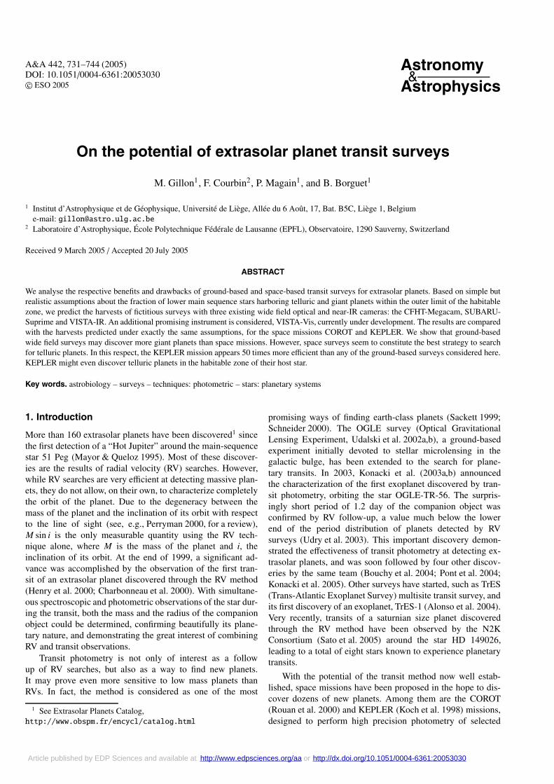
Fig. 1. Density of Lower Main Sequence Stars (LMSS) spectral sub-types in the solar neighborhood, estimated from the Gliese (1991) andZakhozhaj (1979) nearby stars catalogues.

subtypes from F0 to M9 as suitable candidates. We refer tothem as Lower Main-Sequence Stars (LMSS).

The galactic plane is the obvious place to look at, in orderto observe simultaneously many LMSS. It is, indeed, the strat-egy adopted in the pioneering work by Mallén-Ornelas et al.(2003). Since the highest possible Signal-to-Noise Ratio (SNR)per exposure is required, fields with minimal reddening areprefered. A best choice consists of fields close to, but not rightin, the galactic plane, with galactic latitudes between 2◦ and 6◦.We have chosen to carry out all our computations for fields witha mean latitude of 4◦, where a representative extinction coeffi-cient is AV = 0.7 mag/kpc (Schlegel et al. 1998).

The projected densities of LMSS at low galactic latitude areestimated from the Gliese & Jarheiss (1991) and the Zakhozhaj(1979) catalogues of stars in the solar neighborhood (seeFig. 1). We assume that these stellar densities also apply to therest of the galactic plane. This is probably a fair approximationas long as the galactic bulge is avoided. The fields we are mod-eling here mainly contain stars belonging to the spiral arms ofour Galaxy.

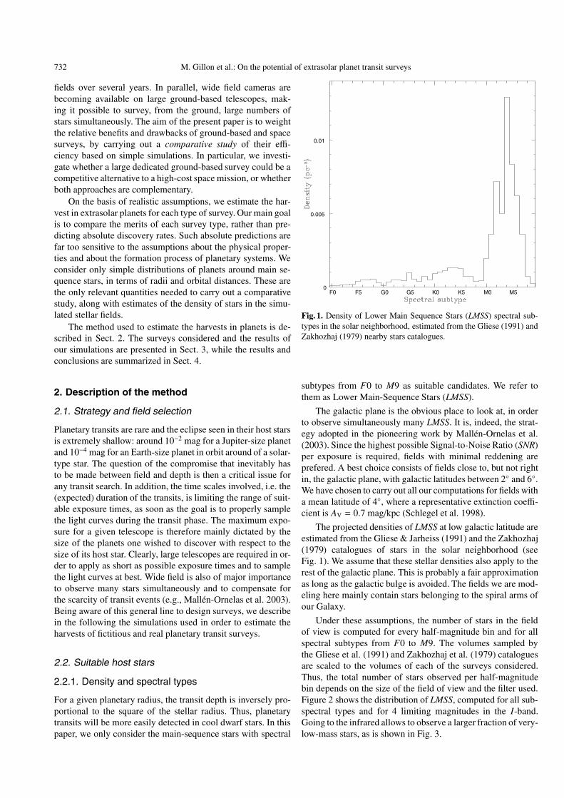
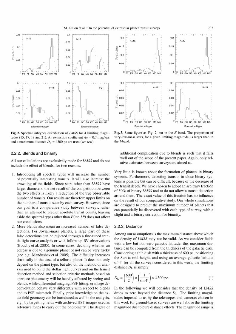
Under these assumptions, the number of stars in the fieldof view is computed for every half-magnitude bin and for allspectral subtypes from F0 to M9. The volumes sampled bythe Gliese et al. (1991) and Zakhozhaj et al. (1979) cataloguesare scaled to the volumes of each of the surveys considered.Thus, the total number of stars observed per half-magnitudebin depends on the size of the field of view and the filter used.Figure 2 shows the distribution of LMSS, computed for all sub-spectral types and for 4 limiting magnitudes in the I-band.Going to the infrared allows to observe a larger fraction of very-low-mass stars, as is shown in Fig. 3.

M. Gillon et al.: On the potential of extrasolar planet transit surveys 733

0

0.05

0.1

0.15

G0 K0 M0F0 F5 G5 K5 M5

I=15

0

0.02

0.04

0.06

0.08

0.1

G0 K0 M0F0 F5 G5 K5 M5

I=17

0

0.02

0.04

0.06

0.08

0.1

G0 K0 M0F0 F5 G5 K5 M5

I=19

Spectral subtype

0

0.02

0.04

0.06

0.08

0.1

G0 K0 M0F0 F5 G5 K5 M5

I=21

Spectral subtype

Fig. 2. Spectral subtypes distribution of LMSS for 4 limiting magni-tudes (15, 17, 19 and 21). An extinction coefficient AV = 0.7 mag/kpcand a maximum distance DL = 4300 pc are used (see text).

2.2.2. Blends and binarity

All our calculations are exclusively made for LMSS and do notinclude the effect of blends, for two reasons:

1. Introducing all spectral types will increase the numberof potentially interesting transits. It will also increase thecrowding of the fields. Since stars other than LMSS havelarger diameters, the net result of the competition betweenthe two effects is likely a reduction of the true observablenumber of transits. Our results are therefore upper limits onthe number of transits seen by each survey. However, sinceour goal is a comparative study between surveys, ratherthan an attempt to predict absolute transit counts, leavingaside the spectral types other than F0 to M9 does not affectour conclusions.

2. More blends also mean an increased number of false de-tections. For Jovian-mass planets, a large part of thesefalse detections can be rejected through a fine-tuned tran-sit light-curve analysis or with follow-up RV observations(Bouchy et al. 2005). In some cases, deciding whether aneclipse is due to a genuine planet or not can be very tricky(see e.g. Mandushev et al. 2005). The difficulty increasesdrastically in the case of a telluric planet. It does not onlydepend on the planet type, but also on the method of anal-ysis used to build the stellar light curves and on the transitdetection method and selection criteria: methods based onaperture photometry will be heavily affected by seeing andblends, while differential imaging, PSF fitting, or image de-convolution behave very differently with respect to blendsand to PSF mismatch. Finally, prior knowledge on the ex-act field geometry can be introduced as well in the analysis,e.g., by targetting fields with archived HST images used asreference maps to carry out the photometry. The degree of

0

0.05

0.1

0.15

0.2

G0 K0 M0F0 F5 G5 K5 M5

K=15

0

0.05

0.1

0.15

0.2

G0 K0 M0F0 F5 G5 K5 M5

K=17

0

0.02

0.04

0.06

0.08

0.1

G0 K0 M0F0 F5 G5 K5 M5

K=19

Spectral subtype

0

0.02

0.04

0.06

0.08

0.1

G0 K0 M0F0 F5 G5 K5 M5

K=21

Spectral subtype

Fig. 3. Same figure as Fig. 2, but in the K-band. The proportion ofvery-low-mass stars, for a given limiting magnitude, is larger than inthe I-band.

additional complication due to blends is such that it fallswell out of the scope of the present paper. Again, only rel-ative estimates between surveys are aimed at.

Very little is known about the formation of planets in binarysystems. Furthermore, detecting transits in close binary sys-tems is possible but can be difficult, because of the decrease ofthe transit depth. We have chosen to adopt an arbitrary fractionof 50% of binary LMSS and to do not allow a transit detectionaround them. The exact value of this fraction has no influenceon the result of our comparative study. Our whole simulationsare designed to predict the maximum number of planets thatcan potentially be discovered with each type of survey, with aslight and arbitrary correction for binarity.

2.2.3. Distance

Among our assumptions is the maximum distance above whichthe density of LMSS may not be valid. As we consider fieldswith a low but non-zero galactic latitude, this maximum dis-tance can be computed from the thickness of the galactic disk.Considering a thin disk with a thickness of 600 pc, positioningthe Sun at mid height, and using an average galactic latitudeof 4◦ for all the surveys considered in this work, the limitingdistance DL is simply:

DL =

(6002

)×(

1sin 4◦

)≈ 4300 pc. (1)

In the following we will consider that the density of LMSSdrops to zero beyond the distance DL. The limiting magni-tudes imposed to us by the telescopes and cameras chosen inthis work for ground-based surveys are well above the limitingmagnitude due to pure distance effects. The magnitude range is

734 M. Gillon et al.: On the potential of extrasolar planet transit surveys

0 5 10 15 200

0.2

0.4

0.6

0.8

1

Radius (Earth radii)

0 0.5 1 1.5 20

0.2

0.4

0.6

0.8

1

Radius (Earth radii)

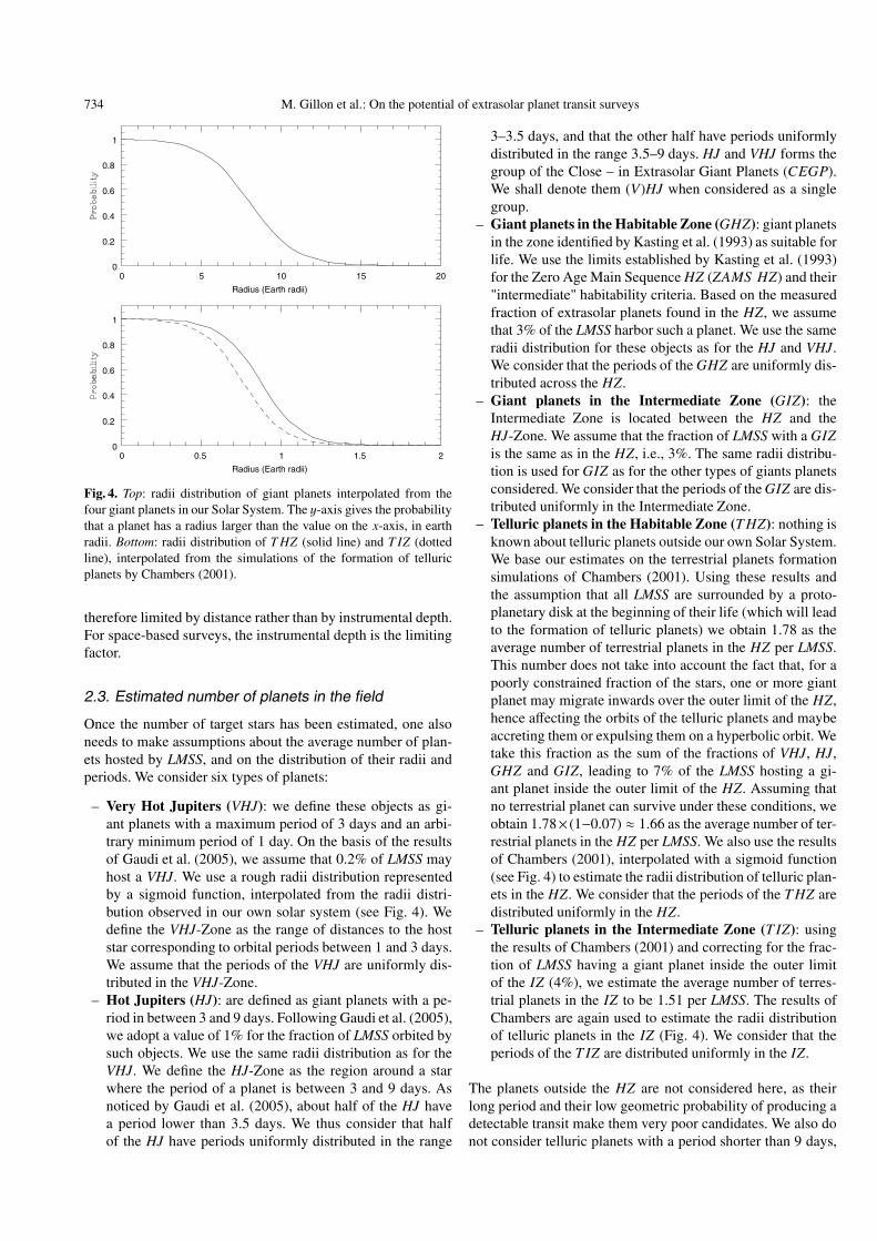
Fig. 4. Top: radii distribution of giant planets interpolated from thefour giant planets in our Solar System. The y-axis gives the probabilitythat a planet has a radius larger than the value on the x-axis, in earthradii. Bottom: radii distribution of T HZ (solid line) and T IZ (dottedline), interpolated from the simulations of the formation of telluricplanets by Chambers (2001).

therefore limited by distance rather than by instrumental depth.For space-based surveys, the instrumental depth is the limitingfactor.

2.3. Estimated number of planets in the field

Once the number of target stars has been estimated, one alsoneeds to make assumptions about the average number of plan-ets hosted by LMSS, and on the distribution of their radii andperiods. We consider six types of planets:

– Very Hot Jupiters (VHJ): we define these objects as gi-ant planets with a maximum period of 3 days and an arbi-trary minimum period of 1 day. On the basis of the resultsof Gaudi et al. (2005), we assume that 0.2% of LMSS mayhost a VHJ. We use a rough radii distribution representedby a sigmoid function, interpolated from the radii distri-bution observed in our own solar system (see Fig. 4). Wedefine the VHJ-Zone as the range of distances to the hoststar corresponding to orbital periods between 1 and 3 days.We assume that the periods of the VHJ are uniformly dis-tributed in the VHJ-Zone.

– Hot Jupiters (HJ): are defined as giant planets with a pe-riod in between 3 and 9 days. Following Gaudi et al. (2005),we adopt a value of 1% for the fraction of LMSS orbited bysuch objects. We use the same radii distribution as for theVHJ. We define the HJ-Zone as the region around a starwhere the period of a planet is between 3 and 9 days. Asnoticed by Gaudi et al. (2005), about half of the HJ havea period lower than 3.5 days. We thus consider that halfof the HJ have periods uniformly distributed in the range

3–3.5 days, and that the other half have periods uniformlydistributed in the range 3.5–9 days. HJ and VHJ forms thegroup of the Close – in Extrasolar Giant Planets (CEGP).We shall denote them (V)HJ when considered as a singlegroup.

– Giant planets in the Habitable Zone (GHZ): giant planetsin the zone identified by Kasting et al. (1993) as suitable forlife. We use the limits established by Kasting et al. (1993)for the Zero Age Main Sequence HZ (ZAMS HZ) and their"intermediate" habitability criteria. Based on the measuredfraction of extrasolar planets found in the HZ, we assumethat 3% of the LMSS harbor such a planet. We use the sameradii distribution for these objects as for the HJ and VHJ.We consider that the periods of the GHZ are uniformly dis-tributed across the HZ.

– Giant planets in the Intermediate Zone (GIZ): theIntermediate Zone is located between the HZ and theHJ-Zone. We assume that the fraction of LMSS with a GIZis the same as in the HZ, i.e., 3%. The same radii distribu-tion is used for GIZ as for the other types of giants planetsconsidered. We consider that the periods of the GIZ are dis-tributed uniformly in the Intermediate Zone.

– Telluric planets in the Habitable Zone (T HZ): nothing isknown about telluric planets outside our own Solar System.We base our estimates on the terrestrial planets formationsimulations of Chambers (2001). Using these results andthe assumption that all LMSS are surrounded by a proto-planetary disk at the beginning of their life (which will leadto the formation of telluric planets) we obtain 1.78 as theaverage number of terrestrial planets in the HZ per LMSS.This number does not take into account the fact that, for apoorly constrained fraction of the stars, one or more giantplanet may migrate inwards over the outer limit of the HZ,hence affecting the orbits of the telluric planets and maybeaccreting them or expulsing them on a hyperbolic orbit. Wetake this fraction as the sum of the fractions of VHJ, HJ,GHZ and GIZ, leading to 7% of the LMSS hosting a gi-ant planet inside the outer limit of the HZ. Assuming thatno terrestrial planet can survive under these conditions, weobtain 1.78× (1−0.07) ≈ 1.66 as the average number of ter-restrial planets in the HZ per LMSS. We also use the resultsof Chambers (2001), interpolated with a sigmoid function(see Fig. 4) to estimate the radii distribution of telluric plan-ets in the HZ. We consider that the periods of the T HZ aredistributed uniformly in the HZ.

– Telluric planets in the Intermediate Zone (T IZ): usingthe results of Chambers (2001) and correcting for the frac-tion of LMSS having a giant planet inside the outer limitof the IZ (4%), we estimate the average number of terres-trial planets in the IZ to be 1.51 per LMSS. The results ofChambers are again used to estimate the radii distributionof telluric planets in the IZ (Fig. 4). We consider that theperiods of the T IZ are distributed uniformly in the IZ.

The planets outside the HZ are not considered here, as theirlong period and their low geometric probability of producing adetectable transit make them very poor candidates. We also donot consider telluric planets with a period shorter than 9 days,

M. Gillon et al.: On the potential of extrasolar planet transit surveys 735

Table 1. Instruments considered in our fictitious ground-based sur-veys.

Instr. Telescope Field Locationdiameter (sq. degrees)

Megacam 3.6 m 0.90 Hawaii (CFHT)Suprime 8.3 m 0.26 Hawaii (Subaru)Vista-IR 4.0 m 1.00 Chile (VLT)Vista-Vis 4.0 m 2.25 Chile (VLT)

because they are not predicted by the simulations of Chambersand because there is no such planet in our own solar system.

Our assumptions about giant planets are empirical, andbased on previous surveys that are certainly biased towards agiven type of planet and orbit and still suffer from low numberstatistics. Furthermore, we assume that the average expectednumber of planets for the four zones we defined earlier are thesame for all spectral subtypes from F0 to M9. This assumptiondoes not have a strong influence on the results given our alreadyrough knowledge of planetary formation, although a metallic-ity dependence on exoplanets population has been emphasized(see e.g. Santos et al. 2004) and low-mass stars tend to be olderon average and have a lower metallicity. The predicted harvestsshould nevertheless be of the right order of magnitude and arecertainly adequate for comparison purposes.

The assumptions made on telluric planets are based on apurely theoretical work. We do not take into account the possi-ble existence of giant planet cores formed in the outer region ofthe disk and that later migrated inwards. These objects, withouta massive primary atmosphere, could consist of large planets ofpure rock and ice. We prefer to remain conservative and to con-sider exclusively planets formed in the more standard scenariothought to be responsible for the formation of planetary sys-tems such our own.

The known weaknesses of the assumptions used in our sim-ulations are not a critical issue for our purpose, which is to com-pare the relative strengths and weaknesses of different transitsurveys rather than to predict actual discovery rates for a givensurvey. Our results may be scaled up and down, but we believethat they remain correct as long as the aim is to carry out com-parative studies.

2.4. Parameters of the instruments chosenfor the fictitious ground-based surveys

Transit searches must combine large field of view, depthand good temporal sampling. Although the range of pos-sible telescope/camera combinations is broad, we have se-lected four instruments that can be considered as representa-tive of the present or soon available astronomical facilities.Three of these instruments are already in use: CFHT-Megacam,Subaru-Suprime, and Vista-IR. The latter one is only proposed:Vista-Vis2 (see Table 1).

For each instrument, we have estimated the SNR and thesaturation magnitude for a range of exposure times, for a fixed

2 See VISTA web site,http://www.vista.ac.uk

airmass (1.6) and typical seeing (1 arcsec). These parametersare computed for different filters, using the Exposure TimeCalculators (ETC) available for Subaru and the CFHT. Thebright cut applied to the magnitude distribution of host starscorresponds to saturation time. The faint cut corresponds to themagnitude of stars that have a SNR < 10, where a shallow tran-sit would not be detected.

For Vista-Vis, we used the information given in the onlineETC of the EMMI camera. This ESO instrument is mounted onthe 3.5 m NTT at La Silla (Chile) and has a throughput similarto Vista, which will also be a 4 m-class telescope. For Vista-IR,we use the information given on the online ETC of the SOFIIR camera of the ESO 3.5 m NTT.

All our estimated SNR are corrected for the extra source ofnoise introduced by stellar variability, following the formula:

SNR2 =SNR1√

1 + (σ∗SNR1)2, (2)

where SNR1 and SNR2 are the SNR before and after taking σ∗into account, the standard deviation of the stellar variability.We adopt σ∗ = 100 ppm as estimated from the solar variabilitywithin a frequency interval that matches our adopted range oftransit durations (Bordé 2003). We consider this same value forevery LMSS spectral subtypes.

2.5. Computation of the harvests and detection criteria

Under all the above assumptions, the expected numbers of tran-sit detections are estimated as follows.

For every spectral subtype F0 to M9, we compute 100 cir-cular orbits for each of the four zones considered, distributedas mentioned in Sect. 2.3. The geometric transit probability foran orbit is given by

Ptr =R∗a, (3)

where R∗ is the radius of the star and a the semi-major axis ofthe planet orbit. For every orbit and for a range of inclinationsand planetary radii, we compute the total crossing-time of thetransit and the duration of the flat part of the light curve, follow-ing the calculation by Mallén-Ornelas et al. (2001). The resultsare then averaged on the inclinations and radii.

A window function is computed for each survey, based onthe total number of nights in the campaign and the visibil-ity of the field each night, in the case of ground-based sur-veys. To take weather effects into account, we assume that for1 night out of 10, no observations are taken at all. In addition,10 chunks of 1 h are randomly removed from the 9 remainingnights to account for technical problem, clouds, or unexpectedoverheads.

We then compute a probability PvisN that a transit is ob-served N times for a specific orbit and a specific LMSS. Wecompute this probability for N varying from 1 to X, where X isthe maximum number of transits we could observe for the samestar during the whole observing season. As the shortest periodconsidered is 1 day, X is simply the duration of the survey indays.

736 M. Gillon et al.: On the potential of extrasolar planet transit surveys

For a specific spectral type and a specific distance, the prob-ability PobsN that a transit occurs N times during the survey andis observable is PobsN = Ptr × PvisN .

We then consider that the observed dimming of a lightcurve can be attributed to a genuine planet only if at least threeeclipses are detected. We define k as the number of transits ob-served during the survey and impose that the SNR of the lightcurve, integrated on the duration of the flat part of the k transitsis at least β time greater than the inverse of transit depth, i.e.

SNR ≥ β√k

(R∗Rp

)2, (4)

where Rp is the planetary radius and R∗ the radius of the hoststar.

In other words, the significance of planetary transits in astellar light curve is β × σ.

We have chosen to adopt β = 9. This value is high enoughto reject the majority of the statistical artifacts. Is is also theone adopted by the OGLE-III team (Udalski, private commu-nication). The value β = 7 is also tested, as it is used in othertransit studies such as in Bordé et al. (2003) for the COROTmission.

For a specific planet transiting k times during the survey,and for a star of a given magnitude and a given radius R∗,Eq. (4) allows a computation of the minimum planetary radiusneeded to get a SNR high enough to allow a statistically signif-icant detection. The relevant radii distribution then leads to adetermination of the probability that the planet has a radius atleast equal to the minimum radius of detection, i.e. the fractionof planets which would produce a dimming strong enough tobe detected.

For every half magnitude bin and for every zone consid-ered, the results are averaged over 100 orbits and multiplied bythe number of stars of each spectral type present in each half-magnitude bin. We then multiply by the fraction of stars ex-pected to host a planet (giant or telluric) in the zone considered,leading to the expected number of planet detections. As a finalstep, we sum the numbers of planets for each half-magnitudebin and spectral subtype, and obtain the total number of detec-tions for each planet type.

3. Results

3.1. Analysis of existing surveys: OGLE-IIIand EXPLORE-I

We have tested our simulations on two existing ground-based surveys, EXPLORE-I (Mallén-Ornelas et al. 2003) andOGLE-III (Udalski et al. 2002a,b, 2004). The goal was to com-pare our predictions to the actual results of these surveys and tocheck the validity of our assumptions. Our main goal remainsthe comparison of existing ground-based surveys to future fic-titious ground-based surveys and to space missions.

3.2. EXPLORE-I

The Extrasolar Planet Occultation Research search lasted11 nights, at the CTIO 4 m telescope, in the I-band with the

Table 2. Results predicted for EXPLORE-I. In the first line, we adoptPvis2 = 0.1 for (V)HJ and Pvis2 = 0 for the other types of planets.The second and third lines involve a PvisN computed assuming goodweather conditions (see text). The values in brackets are for β = 7, andthe others correspond to β = 9.

Weather conditions VHJ HJReal conditions (k = 2) 0.4 (0.5) 1.2 (1.5)Good weather (k ≥ 2) 3.4 (4.2) 2.8 (3.4)Good weather (k ≥ 3) 2.2 (2.7) 0.7 (0.9)

mosaic II camera. It concentrated on one single 0.36 deg2 fieldnear the galactic plane (l = −27.8 ◦, b = −2.7 ◦) containing∼100 000 stars down to I = 18.2 and ∼350 000 stars down toI = 21.0. Poor weather conditions led to a degraded windowfunction, affecting the probability Pvis2 to detect two transits ofthe same planet. Pvis2 was estimated as 0.1 for (V)HJ by theEXPLORE team (Mallén-Ornelas, private communication).

The typical exposure time was 60 s, and the detector readtime plus overhead amounted to 101 s. The analysis of the datais not completed, and no final detection criterion has been de-cided up to now (Mallén-Ornelas, private communication). Noexoplanet transit has been discovered so far.

Following the simulations presented in this paper, withPvis2 = 0.1 for (V)HJ (and PvisN>2 set to 0, i.e. assuming thatthe probability to detect three transits of the same planet isnegligible), we compute the expected harvest for EXPLORE-I,given its true weather conditions. We also compute the harvestfor good weather conditions, i.e. without fixing PvisN but esti-mating it according to the method described in Sect. 2.5. Ourresults for the two detection criteria (β = 9 and β = 7) arepresented in Table 2.

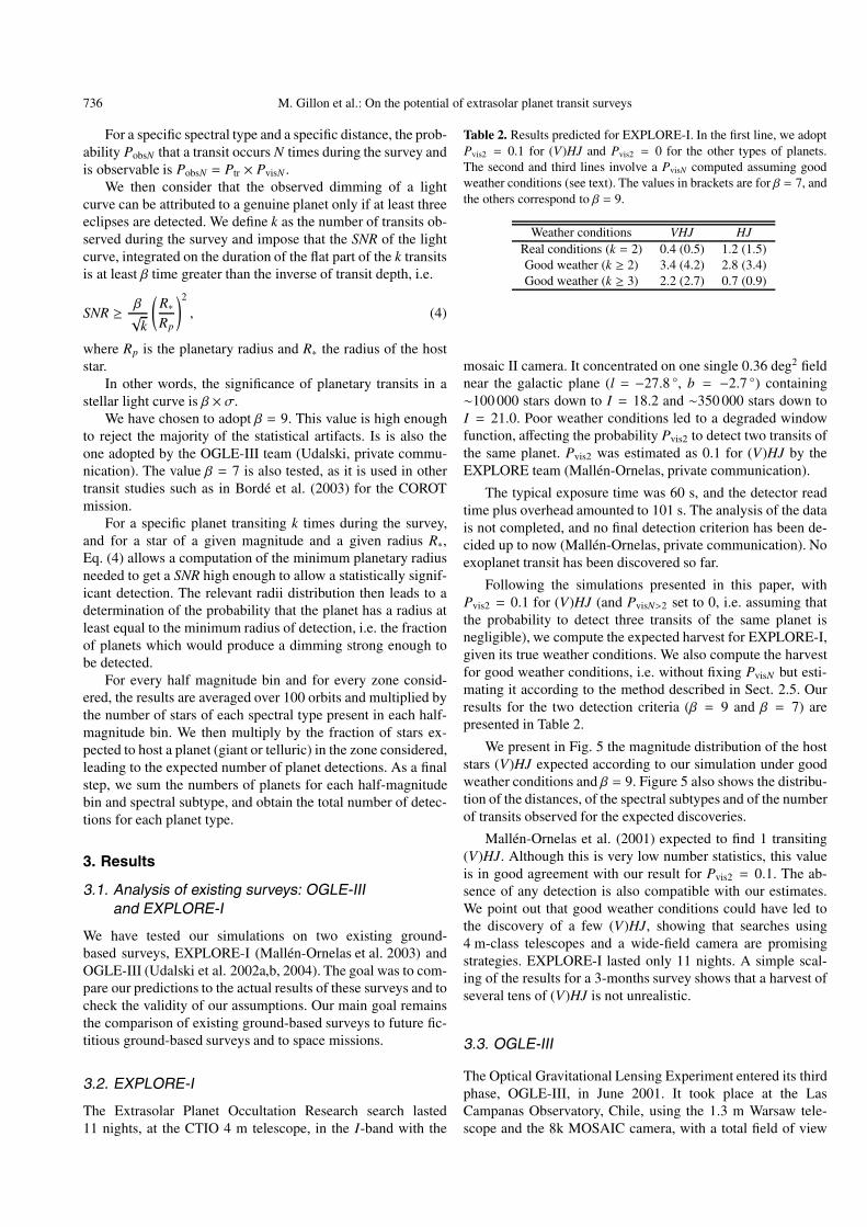
We present in Fig. 5 the magnitude distribution of the hoststars (V)HJ expected according to our simulation under goodweather conditions and β = 9. Figure 5 also shows the distribu-tion of the distances, of the spectral subtypes and of the numberof transits observed for the expected discoveries.

Mallén-Ornelas et al. (2001) expected to find 1 transiting(V)HJ. Although this is very low number statistics, this valueis in good agreement with our result for Pvis2 = 0.1. The ab-sence of any detection is also compatible with our estimates.We point out that good weather conditions could have led tothe discovery of a few (V)HJ, showing that searches using4 m-class telescopes and a wide-field camera are promisingstrategies. EXPLORE-I lasted only 11 nights. A simple scal-ing of the results for a 3-months survey shows that a harvest ofseveral tens of (V)HJ is not unrealistic.

3.3. OGLE-III

The Optical Gravitational Lensing Experiment entered its thirdphase, OGLE-III, in June 2001. It took place at the LasCampanas Observatory, Chile, using the 1.3 m Warsaw tele-scope and the 8k MOSAIC camera, with a total field of view

M. Gillon et al.: On the potential of extrasolar planet transit surveys 737

4 6 8 10 120

0.5

1

1.5

2

Number of transits

Total = 2.92

0 1000 2000 3000 40000

0.1

0.2

0.3

0.4

0.5

Distance (pc)

Total = 2.92

16 18 20 220

0.1

0.2

0.3

0.4

0.5

I

Total = 2.92

0

0.05

0.1

0.15

0.2Total = 2.92

Spectral subtype

Fig. 5. Distribution of the expected number of (V)HJ for EXPLORE-I(with good weather conditions) as a function of the number of tran-sits observed (upper left), of the distance (upper right), the magnitude(bottom left) and the spectral subtype (bottom right) of the host star.The irregular shape of the histogram as a function of distance is anartificial effect caused by the rounding off of the stellar magnitudes tothe nearest integer or half-integer.

of 0.34 deg2. All observations were made through the I filter.Four surveys have been carried out so far:

– OGLE-III-1 (June 12 to July 28, 2001). More than 800 im-ages of three fields in the direction of the galactic bulgewere collected within 32 nights. The exposure time was120 s, and each field was observed every 12 min.

– OGLE-III-2 (February 17 to May 22, 2002). More than1100 images of three fields located in the Carina regionof the galactic disk were collected in 76 nights. The expo-sure time was 180 s, and the temporal resolution was about15 min.

– OGLE-III-3 (February 12 to March 26, 2003). The photo-metric data were collected during 39 nights spanning the43 days of the survey. Three fields of the galactic disk wereobserved with a time resolution of about 15 min. The expo-sure time was 180 s.

– OGLE-III-4. Starting on March 25, 2003, this survey col-lected its main photometric material until middle May2003, but observations were also collected until July 25,2003 with sparse temporal sampling. Three fields of thegalactic disk were observed with the same exposure timeand resolution as the two previous surveys.

Using the observation windows and instrumental parametersof these 4 surveys (A. Udalski, private communication), wehave computed the expected harvests for the two detection cri-teria (see Table 3). OGLE-III-1 and OGLE-III-2 have yield 5genuine extrasolar planets so far. OGLE-III-3 and OGLE-III-4have discovered 40 transiting companions, but follow-up

4 6 8 10 120

0.5

1

1.5

Number of transits

Total = 4.14

0 1000 2000 3000 40000

0.05

0.1

0.15

0.2

0.25

Distance (pc)

Total = 4.14

14 16 18 200

0.2

0.4

0.6

0.8

I

Total = 4.14

0

0.1

0.2

0.3Total = 4.14

Spectral subtype

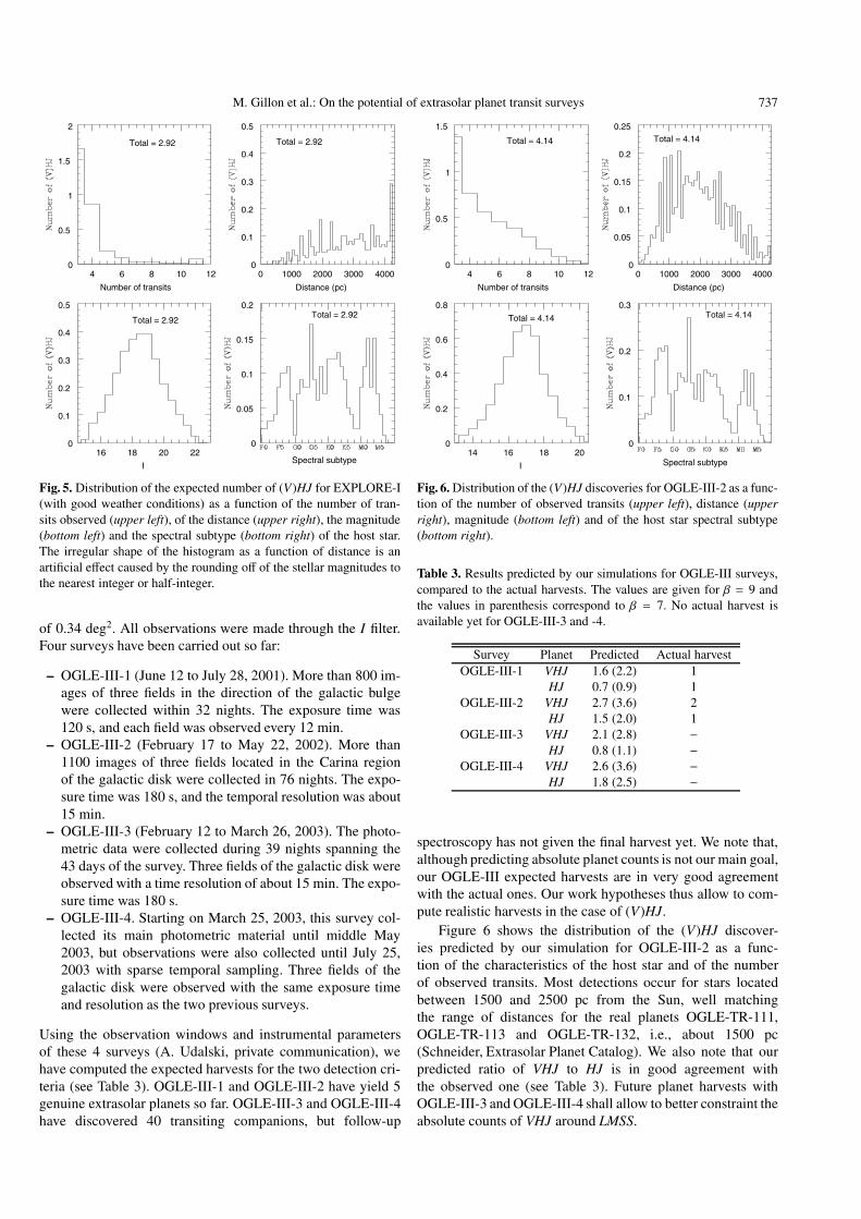
Fig. 6. Distribution of the (V)HJ discoveries for OGLE-III-2 as a func-tion of the number of observed transits (upper left), distance (upperright), magnitude (bottom left) and of the host star spectral subtype(bottom right).

Table 3. Results predicted by our simulations for OGLE-III surveys,compared to the actual harvests. The values are given for β = 9 andthe values in parenthesis correspond to β = 7. No actual harvest isavailable yet for OGLE-III-3 and -4.

Survey Planet Predicted Actual harvestOGLE-III-1 VHJ 1.6 (2.2) 1

HJ 0.7 (0.9) 1OGLE-III-2 VHJ 2.7 (3.6) 2

HJ 1.5 (2.0) 1OGLE-III-3 VHJ 2.1 (2.8) −

HJ 0.8 (1.1) −OGLE-III-4 VHJ 2.6 (3.6) −

HJ 1.8 (2.5) −

spectroscopy has not given the final harvest yet. We note that,although predicting absolute planet counts is not our main goal,our OGLE-III expected harvests are in very good agreementwith the actual ones. Our work hypotheses thus allow to com-pute realistic harvests in the case of (V)HJ.

Figure 6 shows the distribution of the (V)HJ discover-ies predicted by our simulation for OGLE-III-2 as a func-tion of the characteristics of the host star and of the numberof observed transits. Most detections occur for stars locatedbetween 1500 and 2500 pc from the Sun, well matchingthe range of distances for the real planets OGLE-TR-111,OGLE-TR-113 and OGLE-TR-132, i.e., about 1500 pc(Schneider, Extrasolar Planet Catalog). We also note that ourpredicted ratio of VHJ to HJ is in good agreement withthe observed one (see Table 3). Future planet harvests withOGLE-III-3 and OGLE-III-4 shall allow to better constraint theabsolute counts of VHJ around LMSS.

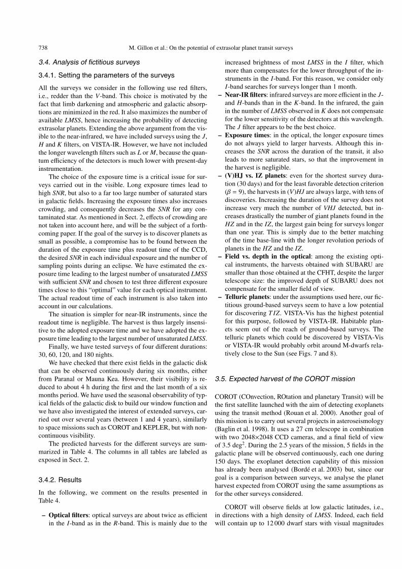
738 M. Gillon et al.: On the potential of extrasolar planet transit surveys

3.4. Analysis of fictitious surveys

3.4.1. Setting the parameters of the surveys

All the surveys we consider in the following use red filters,i.e., redder than the V-band. This choice is motivated by thefact that limb darkening and atmospheric and galactic absorp-tions are minimized in the red. It also maximizes the number ofavailable LMSS, hence increasing the probability of detectingextrasolar planets. Extending the above argument from the vis-ible to the near-infrared, we have included surveys using the J,H and K filters, on VISTA-IR. However, we have not includedthe longer wavelength filters such as L or M, because the quan-tum efficiency of the detectors is much lower with present-dayinstrumentation.

The choice of the exposure time is a critical issue for sur-veys carried out in the visible. Long exposure times lead tohigh SNR, but also to a far too large number of saturated starsin galactic fields. Increasing the exposure times also increasescrowding, and consequently decreases the SNR for any con-taminated star. As mentioned in Sect. 2, effects of crowding arenot taken into account here, and will be the subject of a forth-coming paper. If the goal of the survey is to discover planets assmall as possible, a compromise has to be found between theduration of the exposure time plus readout time of the CCD,the desired SNR in each individual exposure and the number ofsampling points during an eclipse. We have estimated the ex-posure time leading to the largest number of unsaturated LMSSwith sufficient SNR and chosen to test three different exposuretimes close to this “optimal” value for each optical instrument.The actual readout time of each instrument is also taken intoaccount in our calculations.

The situation is simpler for near-IR instruments, since thereadout time is negligible. The harvest is thus largely insensi-tive to the adopted exposure time and we have adopted the ex-posure time leading to the largest number of unsaturated LMSS.

Finally, we have tested surveys of four different durations:30, 60, 120, and 180 nights.

We have checked that there exist fields in the galactic diskthat can be observed continuously during six months, eitherfrom Paranal or Mauna Kea. However, their visibility is re-duced to about 4 h during the first and the last month of a sixmonths period. We have used the seasonal observability of typ-ical fields of the galactic disk to build our window function andwe have also investigated the interest of extended surveys, car-ried out over several years (between 1 and 4 years), similarlyto space missions such as COROT and KEPLER, but with non-continuous visibility.

The predicted harvests for the different surveys are sum-marized in Table 4. The columns in all tables are labeled asexposed in Sect. 2.

3.4.2. Results

In the following, we comment on the results presented inTable 4.

– Optical filters: optical surveys are about twice as efficientin the I-band as in the R-band. This is mainly due to the

increased brightness of most LMSS in the I filter, whichmore than compensates for the lower throughput of the in-struments in the I-band. For this reason, we consider onlyI-band searches for surveys longer than 1 month.

– Near-IR filters: infrared surveys are more efficient in the J-and H-bands than in the K-band. In the infrared, the gainin the number of LMSS observed in K does not compensatefor the lower sensitivity of the detectors at this wavelength.The J filter appears to be the best choice.

– Exposure times: in the optical, the longer exposure timesdo not always yield to larger harvests. Although this in-creases the SNR across the duration of the transit, it alsoleads to more saturated stars, so that the improvement inthe harvest is negligible.

– (V)HJ vs. IZ planets: even for the shortest survey dura-tion (30 days) and for the least favorable detection criterion(β = 9), the harvests in (V)HJ are always large, with tens ofdiscoveries. Increasing the duration of the survey does notincrease very much the number of VHJ detected, but in-creases drastically the number of giant planets found in theHZ and in the IZ, the largest gain being for surveys longerthan one year. This is simply due to the better matchingof the time base-line with the longer revolution periods ofplanets in the HZ and the IZ.

– Field vs. depth in the optical: among the existing opti-cal instruments, the harvests obtained with SUBARU aresmaller than those obtained at the CFHT, despite the largertelescope size: the improved depth of SUBARU does notcompensate for the smaller field of view.

– Telluric planets: under the assumptions used here, our fic-titious ground-based surveys seem to have a low potentialfor discovering T IZ. VISTA-Vis has the highest potentialfor this purpose, followed by VISTA-IR. Habitable plan-ets seem out of the reach of ground-based surveys. Thetelluric planets which could be discovered by VISTA-Visor VISTA-IR would probably orbit around M-dwarfs rela-tively close to the Sun (see Figs. 7 and 8).

3.5. Expected harvest of the COROT mission

COROT (COnvection, ROtation and planetary Transit) will bethe first satellite launched with the aim of detecting exoplanetsusing the transit method (Rouan et al. 2000). Another goal ofthis mission is to carry out several projects in asteroseismology(Baglin et al. 1998). It uses a 27 cm telescope in combinationwith two 2048×2048 CCD cameras, and a final field of viewof 3.5 deg2. During the 2.5 years of the mission, 5 fields in thegalactic plane will be observed continuously, each one during150 days. The exoplanet detection capability of this missionhas already been analysed (Bordé et al. 2003) but, since ourgoal is a comparison between surveys, we analyse the planetharvest expected from COROT using the same assumptions asfor the other surveys considered.

COROT will observe fields at low galactic latitudes, i.e.,in directions with a high density of LMSS. Indeed, each fieldwill contain up to 12 000 dwarf stars with visual magnitudes

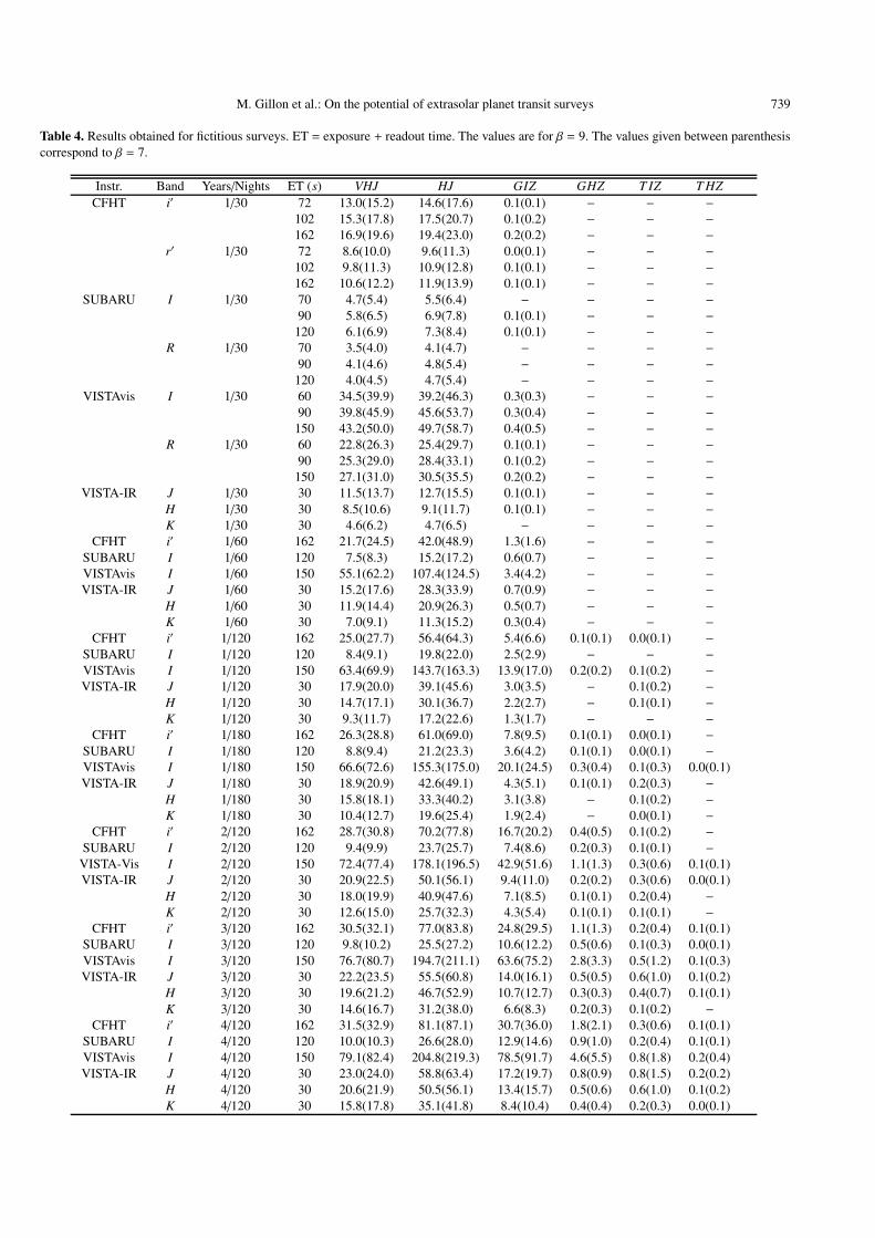
M. Gillon et al.: On the potential of extrasolar planet transit surveys 739

Table 4. Results obtained for fictitious surveys. ET = exposure + readout time. The values are for β = 9. The values given between parenthesiscorrespond to β = 7.

Instr. Band Years/Nights ET (s) VHJ HJ GIZ GHZ T IZ T HZCFHT i′ 1/30 72 13.0(15.2) 14.6(17.6) 0.1(0.1) − − −

102 15.3(17.8) 17.5(20.7) 0.1(0.2) − − −162 16.9(19.6) 19.4(23.0) 0.2(0.2) − − −

r′ 1/30 72 8.6(10.0) 9.6(11.3) 0.0(0.1) − − −102 9.8(11.3) 10.9(12.8) 0.1(0.1) − − −162 10.6(12.2) 11.9(13.9) 0.1(0.1) − − −

SUBARU I 1/30 70 4.7(5.4) 5.5(6.4) − − − −90 5.8(6.5) 6.9(7.8) 0.1(0.1) − − −

120 6.1(6.9) 7.3(8.4) 0.1(0.1) − − −R 1/30 70 3.5(4.0) 4.1(4.7) − − − −

90 4.1(4.6) 4.8(5.4) − − − −120 4.0(4.5) 4.7(5.4) − − − −

VISTAvis I 1/30 60 34.5(39.9) 39.2(46.3) 0.3(0.3) − − −90 39.8(45.9) 45.6(53.7) 0.3(0.4) − − −

150 43.2(50.0) 49.7(58.7) 0.4(0.5) − − −R 1/30 60 22.8(26.3) 25.4(29.7) 0.1(0.1) − − −

90 25.3(29.0) 28.4(33.1) 0.1(0.2) − − −150 27.1(31.0) 30.5(35.5) 0.2(0.2) − − −

VISTA-IR J 1/30 30 11.5(13.7) 12.7(15.5) 0.1(0.1) − − −H 1/30 30 8.5(10.6) 9.1(11.7) 0.1(0.1) − − −K 1/30 30 4.6(6.2) 4.7(6.5) − − − −

CFHT i′ 1/60 162 21.7(24.5) 42.0(48.9) 1.3(1.6) − − −SUBARU I 1/60 120 7.5(8.3) 15.2(17.2) 0.6(0.7) − − −VISTAvis I 1/60 150 55.1(62.2) 107.4(124.5) 3.4(4.2) − − −VISTA-IR J 1/60 30 15.2(17.6) 28.3(33.9) 0.7(0.9) − − −

H 1/60 30 11.9(14.4) 20.9(26.3) 0.5(0.7) − − −K 1/60 30 7.0(9.1) 11.3(15.2) 0.3(0.4) − − −

CFHT i′ 1/120 162 25.0(27.7) 56.4(64.3) 5.4(6.6) 0.1(0.1) 0.0(0.1) −SUBARU I 1/120 120 8.4(9.1) 19.8(22.0) 2.5(2.9) − − −VISTAvis I 1/120 150 63.4(69.9) 143.7(163.3) 13.9(17.0) 0.2(0.2) 0.1(0.2) −VISTA-IR J 1/120 30 17.9(20.0) 39.1(45.6) 3.0(3.5) − 0.1(0.2) −

H 1/120 30 14.7(17.1) 30.1(36.7) 2.2(2.7) − 0.1(0.1) −K 1/120 30 9.3(11.7) 17.2(22.6) 1.3(1.7) − − −

CFHT i′ 1/180 162 26.3(28.8) 61.0(69.0) 7.8(9.5) 0.1(0.1) 0.0(0.1) −SUBARU I 1/180 120 8.8(9.4) 21.2(23.3) 3.6(4.2) 0.1(0.1) 0.0(0.1) −VISTAvis I 1/180 150 66.6(72.6) 155.3(175.0) 20.1(24.5) 0.3(0.4) 0.1(0.3) 0.0(0.1)VISTA-IR J 1/180 30 18.9(20.9) 42.6(49.1) 4.3(5.1) 0.1(0.1) 0.2(0.3) −

H 1/180 30 15.8(18.1) 33.3(40.2) 3.1(3.8) − 0.1(0.2) −K 1/180 30 10.4(12.7) 19.6(25.4) 1.9(2.4) − 0.0(0.1) −

CFHT i′ 2/120 162 28.7(30.8) 70.2(77.8) 16.7(20.2) 0.4(0.5) 0.1(0.2) −SUBARU I 2/120 120 9.4(9.9) 23.7(25.7) 7.4(8.6) 0.2(0.3) 0.1(0.1) −

VISTA-Vis I 2/120 150 72.4(77.4) 178.1(196.5) 42.9(51.6) 1.1(1.3) 0.3(0.6) 0.1(0.1)VISTA-IR J 2/120 30 20.9(22.5) 50.1(56.1) 9.4(11.0) 0.2(0.2) 0.3(0.6) 0.0(0.1)

H 2/120 30 18.0(19.9) 40.9(47.6) 7.1(8.5) 0.1(0.1) 0.2(0.4) −K 2/120 30 12.6(15.0) 25.7(32.3) 4.3(5.4) 0.1(0.1) 0.1(0.1) −

CFHT i′ 3/120 162 30.5(32.1) 77.0(83.8) 24.8(29.5) 1.1(1.3) 0.2(0.4) 0.1(0.1)SUBARU I 3/120 120 9.8(10.2) 25.5(27.2) 10.6(12.2) 0.5(0.6) 0.1(0.3) 0.0(0.1)VISTAvis I 3/120 150 76.7(80.7) 194.7(211.1) 63.6(75.2) 2.8(3.3) 0.5(1.2) 0.1(0.3)VISTA-IR J 3/120 30 22.2(23.5) 55.5(60.8) 14.0(16.1) 0.5(0.5) 0.6(1.0) 0.1(0.2)

H 3/120 30 19.6(21.2) 46.7(52.9) 10.7(12.7) 0.3(0.3) 0.4(0.7) 0.1(0.1)K 3/120 30 14.6(16.7) 31.2(38.0) 6.6(8.3) 0.2(0.3) 0.1(0.2) −

CFHT i′ 4/120 162 31.5(32.9) 81.1(87.1) 30.7(36.0) 1.8(2.1) 0.3(0.6) 0.1(0.1)SUBARU I 4/120 120 10.0(10.3) 26.6(28.0) 12.9(14.6) 0.9(1.0) 0.2(0.4) 0.1(0.1)VISTAvis I 4/120 150 79.1(82.4) 204.8(219.3) 78.5(91.7) 4.6(5.5) 0.8(1.8) 0.2(0.4)VISTA-IR J 4/120 30 23.0(24.0) 58.8(63.4) 17.2(19.7) 0.8(0.9) 0.8(1.5) 0.2(0.2)

H 4/120 30 20.6(21.9) 50.5(56.1) 13.4(15.7) 0.5(0.6) 0.6(1.0) 0.1(0.2)K 4/120 30 15.8(17.8) 35.1(41.8) 8.4(10.4) 0.4(0.4) 0.2(0.3) 0.0(0.1)

740 M. Gillon et al.: On the potential of extrasolar planet transit surveys

12 14 16 18 200

0.1

0.2

0.3

0.4

J

Ntot = 1.7

0

0.1

0.2

0.3

0.4

G0 K0 M0F0 F5 G5 K5 M5Spectral subtype

Ntot = 1.7

0 500 1000 15000

0.1

0.2

0.3

0.4

0.5

Distance (pc)

Ntot = 1.7

0 10 20 30 400

0.05

0.1

0.15

0.2

Number of transits

Ntot = 1.7

Fig. 7. Distribution of predicted telluric planet discoveries (β = 7) forVISTA-IR and the 4-years J-band survey, as a function of the num-ber of observed transits (upper left), distance (upper right), magnitude(bottom left) and of the host star spectral subtype (bottom right).

16 18 20 220

0.1

0.2

0.3

0.4

I

Ntot = 2.2

0

0.1

0.2

0.3

0.4

0.5

G0 K0 M0F0 F5 G5 K5 M5Spectral subtype

Ntot = 2.2

0 500 1000 15000

0.2

0.4

0.6

Distance (pc)

Ntot = 2.2

0 10 20 30 400

0.05

0.1

0.15

0.2

0.25

Number of transits

Ntot = 2.2

Fig. 8. Same as Fig. 7 but for VISTA-Vis and 4 years of observationthrough the I filter.

between V = 11 and V = 16.5. The exposure time will be31.7 s, without any filter.

We use the expected number of photoelectrons per expo-sure for every magnitude bin between V = 11 and V = 16.5 aswell as the different noise contributions given on the COROTweb site3 and in Bordé (2003) to compute the theoretical SNRper exposure. Using in addition the duration of one field obser-vation (150 days continuously), and multiplying the obtained

3 http://www.astrsp-mrs.fr/projets/exoplan/corot/

0 50 100 1500

1

2

3

Number of transits

Total = 47.19

0 500 1000 1500 2000 25000

1

2

3

4

Distance (pc)

Total = 47.19

12 14 160

5

10

15

V

Total = 47.19

0

1

2

3

4

5

Total = 47.19

Spectral subtype

Fig. 9. Distribution of predicted planets (all types included) discover-ies using β = 7 for the COROT mission, as a function of the number ofobserved transits (upper left), distance (upper right), magnitude (bot-tom left) and of the host spectral subtype (bottom right).

0 5 10 150

0.005

0.01

0.015

0.02

0.025

Number of transits

Total = 0.14

0 200 400 6000

0.02

0.04

0.06

Distance (pc)

Total = 0.14

12 14 160

0.01

0.02

0.03

0.04

V

Total = 0.14

0

0.005

0.01

0.015

Total = 0.14

Spectral subtype

Fig. 10. Same as Fig. 9 but for telluric planets.

harvest by 5 to take into account the 5 fields that will be mon-itored, we compute the harvests presented in Table 5. The dis-tributions of the total number of planets detected for β = 7as a function of the characteristics of the host stars and of thenumber of transits observed are shown in Figs. 9 and 10 (T IZ).Figure 11 shows the distribution of the LMSS as a function oftheir magnitude in the V-band, for a typical field observed byCOROT.

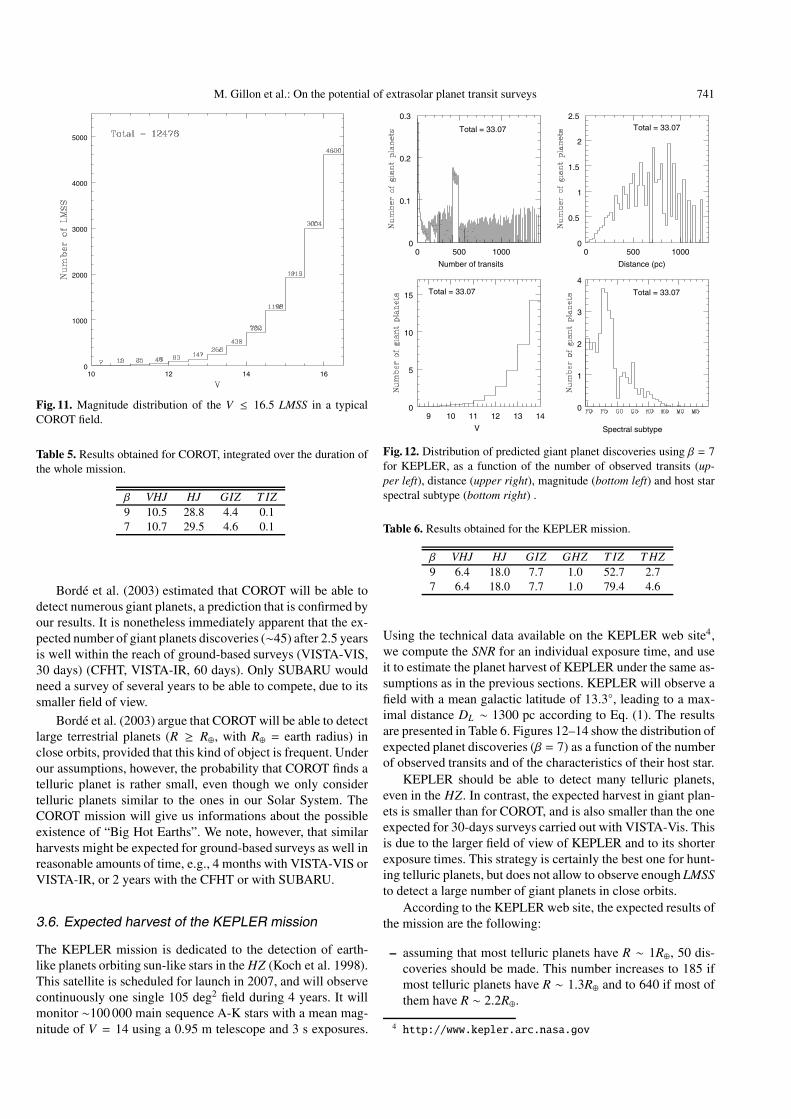
M. Gillon et al.: On the potential of extrasolar planet transit surveys 741

10 12 14 160

1000

2000

3000

4000

5000

Fig. 11. Magnitude distribution of the V ≤ 16.5 LMSS in a typicalCOROT field.

Table 5. Results obtained for COROT, integrated over the duration ofthe whole mission.

β VHJ HJ GIZ T IZ9 10.5 28.8 4.4 0.17 10.7 29.5 4.6 0.1

Bordé et al. (2003) estimated that COROT will be able todetect numerous giant planets, a prediction that is confirmed byour results. It is nonetheless immediately apparent that the ex-pected number of giant planets discoveries (∼45) after 2.5 yearsis well within the reach of ground-based surveys (VISTA-VIS,30 days) (CFHT, VISTA-IR, 60 days). Only SUBARU wouldneed a survey of several years to be able to compete, due to itssmaller field of view.

Bordé et al. (2003) argue that COROT will be able to detectlarge terrestrial planets (R ≥ R⊕, with R⊕ = earth radius) inclose orbits, provided that this kind of object is frequent. Underour assumptions, however, the probability that COROT finds atelluric planet is rather small, even though we only considertelluric planets similar to the ones in our Solar System. TheCOROT mission will give us informations about the possibleexistence of “Big Hot Earths”. We note, however, that similarharvests might be expected for ground-based surveys as well inreasonable amounts of time, e.g., 4 months with VISTA-VIS orVISTA-IR, or 2 years with the CFHT or with SUBARU.

3.6. Expected harvest of the KEPLER mission

The KEPLER mission is dedicated to the detection of earth-like planets orbiting sun-like stars in the HZ (Koch et al. 1998).This satellite is scheduled for launch in 2007, and will observecontinuously one single 105 deg2 field during 4 years. It willmonitor ∼100 000 main sequence A-K stars with a mean mag-nitude of V = 14 using a 0.95 m telescope and 3 s exposures.

0 500 10000

0.1

0.2

0.3

Number of transits

Total = 33.07

0 500 10000

0.5

1

1.5

2

2.5

Distance (pc)

Total = 33.07

9 10 11 12 13 140

5

10

15

V

Total = 33.07

0

1

2

3

4

Total = 33.07

Spectral subtype

Fig. 12. Distribution of predicted giant planet discoveries using β = 7for KEPLER, as a function of the number of observed transits (up-per left), distance (upper right), magnitude (bottom left) and host starspectral subtype (bottom right) .

Table 6. Results obtained for the KEPLER mission.

β VHJ HJ GIZ GHZ T IZ T HZ9 6.4 18.0 7.7 1.0 52.7 2.77 6.4 18.0 7.7 1.0 79.4 4.6

Using the technical data available on the KEPLER web site4,we compute the SNR for an individual exposure time, and useit to estimate the planet harvest of KEPLER under the same as-sumptions as in the previous sections. KEPLER will observe afield with a mean galactic latitude of 13.3◦, leading to a max-imal distance DL ∼ 1300 pc according to Eq. (1). The resultsare presented in Table 6. Figures 12–14 show the distribution ofexpected planet discoveries (β = 7) as a function of the numberof observed transits and of the characteristics of their host star.

KEPLER should be able to detect many telluric planets,even in the HZ. In contrast, the expected harvest in giant plan-ets is smaller than for COROT, and is also smaller than the oneexpected for 30-days surveys carried out with VISTA-Vis. Thisis due to the larger field of view of KEPLER and to its shorterexposure times. This strategy is certainly the best one for hunt-ing telluric planets, but does not allow to observe enough LMSSto detect a large number of giant planets in close orbits.

According to the KEPLER web site, the expected results ofthe mission are the following:

– assuming that most telluric planets have R ∼ 1R⊕, 50 dis-coveries should be made. This number increases to 185 ifmost telluric planets have R ∼ 1.3R⊕ and to 640 if most ofthem have R ∼ 2.2R⊕.

4 http://www.kepler.arc.nasa.gov

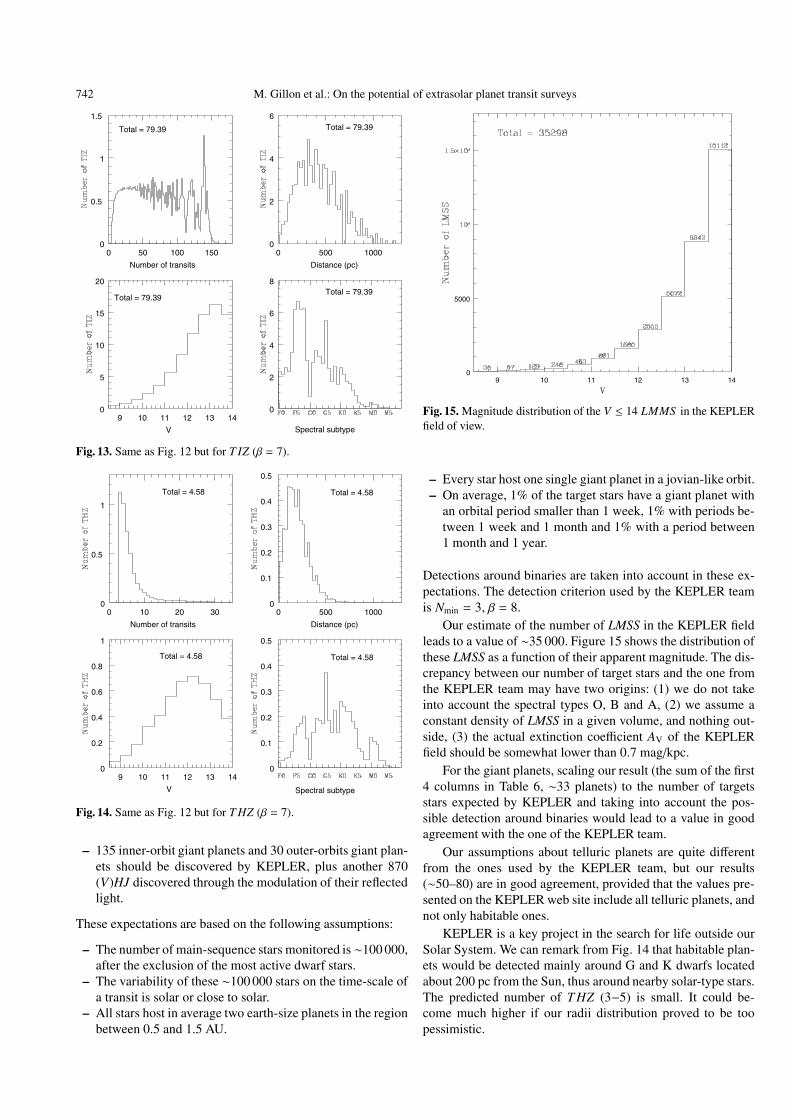
742 M. Gillon et al.: On the potential of extrasolar planet transit surveys

0 50 100 1500

0.5

1

1.5

Number of transits

Total = 79.39

0 500 10000

2

4

6

Distance (pc)

Total = 79.39

9 10 11 12 13 140

5

10

15

20

V

Total = 79.39

0

2

4

6

8Total = 79.39

Spectral subtype

Fig. 13. Same as Fig. 12 but for T IZ (β = 7).

0 10 20 300

0.5

1

Number of transits

Total = 4.58

0 500 10000

0.1

0.2

0.3

0.4

0.5

Distance (pc)

Total = 4.58

9 10 11 12 13 140

0.2

0.4

0.6

0.8

1

V

Total = 4.58

0

0.1

0.2

0.3

0.4

0.5

Total = 4.58

Spectral subtype

Fig. 14. Same as Fig. 12 but for T HZ (β = 7).

– 135 inner-orbit giant planets and 30 outer-orbits giant plan-ets should be discovered by KEPLER, plus another 870(V)HJ discovered through the modulation of their reflectedlight.

These expectations are based on the following assumptions:

– The number of main-sequence stars monitored is ∼100 000,after the exclusion of the most active dwarf stars.

– The variability of these ∼100 000 stars on the time-scale ofa transit is solar or close to solar.

– All stars host in average two earth-size planets in the regionbetween 0.5 and 1.5 AU.

9 10 11 12 13 140

5000

Fig. 15. Magnitude distribution of the V ≤ 14 LMMS in the KEPLERfield of view.

– Every star host one single giant planet in a jovian-like orbit.– On average, 1% of the target stars have a giant planet with

an orbital period smaller than 1 week, 1% with periods be-tween 1 week and 1 month and 1% with a period between1 month and 1 year.

Detections around binaries are taken into account in these ex-pectations. The detection criterion used by the KEPLER teamis Nmin = 3, β = 8.

Our estimate of the number of LMSS in the KEPLER fieldleads to a value of ∼35 000. Figure 15 shows the distribution ofthese LMSS as a function of their apparent magnitude. The dis-crepancy between our number of target stars and the one fromthe KEPLER team may have two origins: (1) we do not takeinto account the spectral types O, B and A, (2) we assume aconstant density of LMSS in a given volume, and nothing out-side, (3) the actual extinction coefficient AV of the KEPLERfield should be somewhat lower than 0.7 mag/kpc.

For the giant planets, scaling our result (the sum of the first4 columns in Table 6, ∼33 planets) to the number of targetsstars expected by KEPLER and taking into account the pos-sible detection around binaries would lead to a value in goodagreement with the one of the KEPLER team.

Our assumptions about telluric planets are quite differentfrom the ones used by the KEPLER team, but our results(∼50–80) are in good agreement, provided that the values pre-sented on the KEPLER web site include all telluric planets, andnot only habitable ones.

KEPLER is a key project in the search for life outside ourSolar System. We can remark from Fig. 14 that habitable plan-ets would be detected mainly around G and K dwarfs locatedabout 200 pc from the Sun, thus around nearby solar-type stars.The predicted number of T HZ (3−5) is small. It could be-come much higher if our radii distribution proved to be toopessimistic.

M. Gillon et al.: On the potential of extrasolar planet transit surveys 743

4. Discussion – conclusions

The main purpose of our simulations was to weight the advan-tages and disadvantages of various ground– and space-basedsearches for exoplanets using the transit method. Tables 2 to 6summarize our results and provide the expected harvest in ex-oplanets for a broad variety of telescope/instrument combina-tions. Our main conclusions are the following:

1. As far as telluric planets in the Habitable Zone are con-cerned, space-based surveys are the only viable option.Such searches remain extremely difficult. They not only re-quire a space instrument, but also a very wide field of view.From space, only the KEPLER mission should be able tofind telluric planets in the Habitable Zone.

2. Telluric planets in the Intermediate Zone are much eas-ier to discover. KEPLER could detect more than 50 ofthem during its four years of observations. Only a few(1–2) TIZ might be discovered from ground-based surveysof the same duration, using VISTA-Vis.

3. Ground-based searches are better than space searches atfinding giant planets. While KEPLER is about as efficientas CFHT at finding giant planets in the Habitable Zone(with 1 expected discovery vs 2), a CFHT search is 4 timesbetter than KEPLER at finding the same planets in theIntermediate Zone, and 5 times better for (V)HJ. This isdue to the much deeper exposures.

Ground-based and space-based transit searches are comple-mentary. Because they go deeper, ground-based searches eas-ily find large planets with a short period, such as (V)HJ.Space searches remain mandatory for telluric planets. AlthoughCOROT might find a few telluric planets, we shall have to waitfor KEPLER to obtain a significant harvest of such objects,provided that they are not significantly less common than ex-pected.

The above results give orders of magnitude estimates forthe expected harvests and allow to emphasize the relative mer-its and drawbacks of the different searches. However, a wordof caution should be given, to avoid over-interpretation of theresults. One need to be aware that:

– Space missions like COROT or KEPLER will defocus theimages, increasing drastically the size of the Point SpreadFunction (PSF). While this will minimize saturation ofbright objects and increase the SNR per image, it might re-sult in severe image blending. The corresponding loss ofefficiency in transit detection will depend on the methodused to post-process the data, as do the effects of blends.This is why we have deliberately chosen not to take PSFconvolution into consideration and to leave it for a futurework. All our estimates are therefore upper limits on theexpected harvests.

– The weather simulations used are very simple, and could besomewhat optimistic. Real weather conditions could lead tolower harvests for ground – based surveys.

– The photometric techniques required for the analysis ofground-based surveys are very efficient in the optical (e.g.,PSF fitting, image subtraction, image deconvolution), but

may be less efficient for near-IR data, where the sky sub-traction is more critical. We therefore expect our near-IRharvest estimates to be slightly more optimistic than the op-tical estimates.

– In the near-IR, second-order extinction effects can have alarge impact on the photometric accuracy (Bailer-Jones &Lamm 2003). Time dependent atmospheric extinction de-pends on the spectral energy distribution of the target. Thismay imply the need to use reference objects of the samespectral type as the target stars and complicate further theanalysis of near-IR data.

Acknowledgements. The authors would like to thank G. Mallén-Ornelas for useful discussions and suggestions, and A. Udalski forproviding informations about OGLE-III. We acknowledge financialsupport from the Prodex-ESA Contract 15448/01/NL/Sfe(IC).

References

Alonso, R., Brown, T. M., Torres, G. et al. 2004, ApJ, 613, L153Baglin, A., et al. 1998, Asteroseismology from space – The COROT

experiment, in New Eyes to See Inside the Sun and Stars, IAU,185, 301

Bailer-Jones, C. A. L., & Lamm, M. 2003, MNRAS, 339, 477Binney, J., & Merrifield, M. 1998, galactic Astronomy (Princeton

University Press)Bordé, P. 2003, Ph.D. Thesis, École doctorale Astronomie &

Astrophysique d’Ile-de-France, Observatoire de Paris, UniversitéPierre et Marie Curie

Bordé, P., Rouan, D., & Léger, A. 2003, A&A, 405, 1137Bouchy, F., Pont, F., Santos, N. C., et al. 2004, A&A, 421, L13Bouchy, F., Pont, F., Melo, C., et al. 2005, A&A, 431, 1105Butler, R. P., et al. 2000, in Planetary Systems in the Universe:

Observation, Formation, and Evolution, ed. A. Penny, P.Artymowicz, A.-M. Lagrange, & S. Russell (San Fransisco: ASP),IAU Symp., 202, in press

Chambers, J. E. 2001, Icarus, 152, 205Charbonneau, D., Brown, T. M., Latham, D. W., & Mayor, M. 2000,

ApJ, 529, L45Gaudi, B. S., Seager, S., & Mallén–Ornelas, G. 2005, ApJ, 623, 472Gliese, W., & Jarheiss, H. 1991, Preliminary Version of the Third

Catalogue of Nearby Stars, Astron. Rechen-Institut, HeidelbergHenry, G. W., Marcy, G. W., Butler, R. P., & Vogt, S. S. 2000, ApJ,

529, L41Kasting, J. F., Whitmire, D. P., & Reynolds, R. T. 1993, Icarus, 101,

108Koch, D., et al. 1998, SPIE Conference 3356, Space Telescope and

Instruments V, 599Konacki, M., Torres, G., Jha, S., & Sasselov, D. D. 2003a, Nature,

421, 507Konacki, M., Torres, G., Sasselov, D. D., & Jha, S. 2003b, ApJ, 597,

1076Konacki, M., Torres, G., Sasselov, D. D., & Jha, S. 2005, ApJ, in pressMallén-Ornelas, G., Seager, S., Yee, H. K. C., et al. 2003, ApJ, 582,

1123Mandushev, G., Torres, G., Latham, D. W., et al. 2005, ApJ, 621, 1061Marcy, G. W., Butler, R. P., Fischer, D. A., & Vogt S. S. 2003, ASP

Conf. Ser., 294Mayor, M., & Queloz, D. 1995, Nature, 378, 355Perryman, M. A. C. 2000, Rep. Prog. Phys., 63, 1209Pont, F., Bouchy, F., Queloz, D., et al. 2004, A&A, 426, 15

744 M. Gillon et al.: On the potential of extrasolar planet transit surveys

Rouan, et al. 2000, Detecting Earth-Uranus class planets with thespace mission COROT. In Darwin and Astronomy – The InfraredSpace Interferometer, ESA SP-451, 221

Santos, N. C., Israelian, G., & Mayor, M. 2004, A&A, 415, 1153Sackett, P. D., 1999, in Planets outside the Solar System: Theory

and Observations (NATO-ASI), ed. J. M. Mariotti & D’Alloin(Dordrecht: Kluwer), 189

Sato, B., et al. 2005, ApJ, acceptedSchlegel, D. J., Finkbeiner, D. P., & Davis, M. 1998, ApJ, 500, 525Schneider, J. 2000, in VLT Opening Ceremony Symposium, ed. F.

Paresce (Berlin: Springer)

Schneider, J. 1996, Extrasolar Planet EncyclopaediaUdalski, A., Paczynski, B., Zebrun, K., et al. 2002a, Acta Astron., 52,

1Udalski, A., Zebrun, K., Szymanski, M., et al. 2002b, Acta Astron.,

52, 115Udalski, A., Szymanski, M. K., Kubiak, M., et al. 2004, Acta Astron.,

54, 313Udry, S., Mayor, M. Clausen, J. V., et al. 2003, A&A, 407, 679Zakhozhaj, V. A., 1979, Catalogue of nearest stars until 10 pc, Vestnik

Khar’kovskogo Universiteta 190, 52