On the performance of early packet discard

ON THE PERFORMANCE OFEARLY PACKET DISCARDMaurizio Casoni and Jonathan S. TurnerComputer Science DepartmentWashington UniversityCampus Box 1045St. Louis, MO [email protected]: +1-314-935-7302Appears in IEEE Journal on Selected Areas of Communications, June 1997, Copyright heldby IEEE. AbstractIn a previous paper [3], one of the authors, gave a worst-case analysis for the Early PacketDiscard (EPD) technique for maintaining packet integrity during overload in ATM switches.This analysis showed that to ensure 100% goodput during overload under worst-case con-ditions, requires a bu�er with enough storage for one maximum length packet from everyactive virtual circuit. This paper re�nes that analysis, using assumptions that are closerto what we expect to see in practice and examines how EPD performs when the bu�er isnot large enough to achieve 100% goodput. We show that 100% goodput can be achievedwith substantially smaller bu�ers than predicted by the worst-case analysis, although therequired bu�er space can be signi�cant when the link speed is substantially higher than therate of the individual virtual circuits. We also show that high goodputs can be achievedwith more modest bu�er sizes, but that EPD exhibits anomalies with respect to bu�ercapacity, in that there are situations in which increasing the amount of bu�ering can causethe goodput to decrease. These results are validated by comparison with simulation.0This work was supported by the ARPA Computing Systems Technology O�ce, NEC, NTT, Samsung, South-western Bell, Sun Microsystems, Tektronix and University of Bologna (I).1

1. IntroductionATM networks carry many di�erent types of tra�c with diverse bandwidth requirements. At oneextreme, there are continuous applications which transmit steadily at �xed rates. At the otherextreme, there are highly bursty applications that transmit large blocks of information at highpeak rates but whose long-term average rates are relatively low. The existence of bursty tra�cmeans that one must either accept low network utilization or the possibility of overload periodsduring which the tra�c sent to some network links exceeds their capacity. In addition, the factthat end-to-end transport protocols send information in packets containing many ATM cells makesthe impact of overload periods worse because the loss of a single cell can lead to the loss andretransmission of the entire transport-level packet. This means that during overload periods, ATMnetworks can experience congestion collapse with the throughput dropping to zero as the loadincreases.It is clear that overload periods will occur in ATM network from time-to-time and so it isimportant to improve their performance during these overload periods. In this paper we focus on amechanism that accepts that cell loss will occur, but attempts to ensure that the available networkcapacity is e�ectively utilized by preserving the integrity of transport level packets during overloadperiods.Early packet discard (EPD) [1] is an ATM bu�er management technique designed ensure highend-to-end throughputs for bursty data applications during overload periods. EPD achieves thisby observing the packet-level structure of each cell stream and discarding entire packets, whenoverload makes it necessary to do so. EPD is only one of several mechanisms that have beenproposed for handling congestion in ATM networks. In particular, rate-based ow control has nowbeen standardized by the ATM Forum to manage congestion for Available Bit Rate (ABR) tra�cstreams [2]. While the use of rate-based ow control reduces the need for techniques like EPD, itdoes not eliminate them, since bu�ers using ABR ow control can still experience overloads duringtransient periods, before rate adjustment mechanisms can react to tra�c changes, and since thesemechanisms will not be applied to Unspeci�ed Bit Rate (UBR) streams. In addition, the expenseof explicit rate control (in terms of memory and control complexity) is likely to limit its applicationto bottleneck points where bandwidth is expensive and scarce (such as at the interface between acampus network and a wide-area network).A previous paper [3] analyzes several packet level discard mechanisms including EPD. Thatanalysis is based on worst-case assumptions that over-state the amount of bu�ering required forhigh e�ective throughputs. In this paper, we re�ne that analysis, using more realistic assumptionsand use this to determine the amount of bu�ering required to achieve 100% goodput (here, wede�ne goodput to be the fraction of the link's capacity that is used to carry complete transportlevel packets). As an example of our results, the worst-case analysis in [3] requires a 120 Kbytebu�er to ensure 100% goodput, for an OC-3 link experiencing a �ve-to-one overload as a result of 15virtual circuits sending 8 Kbyte packets at a rate of 50 Mb/s each. The new analysis shows that a 20Kbyte bu�er is su�cient to ensure 100% goodput in this case. At the same time, our analysis alsoshows that large bu�ers are needed for 100% goodput if the individual virtual circuits contributingto the overload are sending data at low rates. So for example, if the �ve-to-one overload in theexample is the result of tra�c from virtual circuits sending at a rate of 1 Mb/s each, then a bu�erof almost 1 Mbyte is needed to ensure 100% goodput. (Of course, when individual virtual circuitshave such small peak rates, the probability of such a large overload is extremely small.)We also study how EPD behaves when the bu�er is not large enough to ensure 100% goodput.2

We �nd that di�erent choices of the bu�er size and threshold placement lead to very di�erent be-haviors. In general, EPD can provide reasonably high goodput even when the bu�ers are relativelysmall, but the behavior is not always intuitively obvious. In particular, we show that increasingbu�er sizes for a �xed o�ered load can result in reducing the goodput, rather than increasing it.As discussed more fully in section 2, the analysis is based on an idealized assumption aboutthe \phase relationships" of packets on di�erent virtual circuits. While the analysis is not exact,comparisons to simulation results (included below) show that it is surprisingly accurate. Theprincipal virtue of our approach is its simplicity and the qualitative insight it provides into thebehavior of EPD. The analysis naturally divides into two distinct cases. The �rst applies whenthe o�ered load is less than twice the link rate, and the second when the o�ered load is more thantwice the link rate. The analyses for the two cases are given in sections 3 and 4, respectively. Insection 5, we give numerical results.2. De�nitions and AssumptionsIn EPD, whenever a virtual circuit begins the transmission of a new packet, the queue controllerdecides whether to accept the packet or to discard it. In particular, if the number of cells in thequeue exceeds a speci�ed threshold, then the packet is not propagated into the queue. If the numberof cells is below the threshold, the packet is propagated. In addition, if any cell of the packet mustbe discarded due to queue over ow, the remainder of that packet is discarded.We consider a homogeneous situation in which r virtual circuits transmit data continually at anormalized rate of � (that is, � is the fraction of the link bandwidth required by a single virtualcircuit), and de�ne the overbooking ratio as r�. For an overloaded link r� > 1. We also assumethat all packets contain ` cells and let k = b1=�c be the maximum number of virtual circuits thatthe link can handle without loss. For simplicity, we will also assume that 1=� is an integer; althoughextension to non-integral values is straightforward, it adds little new information and obscures thekey issues. We let B denote the number of cells the bu�er can contain, and let b denote the thresholdlevel. The values of b and B � b largely determine the goodput that it is possible to achieve on alink that has a bu�er managed by EPD. If both values are large enough, we have 100% goodput.If one or both is too small, we may have bu�er over ow (that is, the bu�er becomes full, causing acell to be discarded), and/or bu�er under ow (the bu�er becomes empty leaving some of the linkbandwidth unused).We de�ne a given virtual circuit to be active if cells from that virtual circuit are being placedin the queue on arrival. Similarly, we de�ne a virtual circuit to be inactive if its cells are beingdiscarded. We assume that the ow of cells on a given virtual circuit is smooth, ignoring thee�ects of jitter caused by variable delays upstream of the bu�er under consideration. Under thisassumption, the bu�er level rises or falls in a predictable way, depending only on the number ofactive virtual circuits.If we observe the number of cells in a queue managed using EPD as a function of time, we willobserve a cyclic behavior in which the number of cells in the queue rises above the threshold, thenas various virtual circuits become inactive (either because they've completed their packets or hadcells discarded), the number of cells stops increasing and drops back down. When it falls belowthreshold, and new packets start arriving at the queue, the bu�er level stops falling and begins torise again. 3

Our prior analysis of early packet discard was based on the worst-case assumption that justbefore every threshold crossing, the �rst cell of a packet arrived on every virtual circuit, meaningthat the next packet boundary was delayed as long as possible after the threshold crossing, leadingto wide excursions around the threshold level. While such worst-case synchronization of packetboundaries is possible, it is hardly likely, and would certainly not be expected to persist over anextended period of time. Hence, in this paper we analyze the queue behavior under another simpleassumption that more closely re ects what might be expected to happen in practice. In particular,we consider the case in which packet boundaries on di�erent virtual circuits are o�set from oneanother by an equal amount, leading to the occurrence of a packet boundary every `=r� cell times.This even o�set assumption is clearly an idealization. In truth, di�erent virtual circuits will haverandom phase relationships relative to one another, leading to uneven spacing of packet boundaries.Consequently, the even o�set assumption is a bit optimistic, but when the number of virtual circuitsis moderately large, this simple model predicts the behavior of EPD with surprising accuracy.3. Performance With Small Overbooking RatiosIn this section we analyze the performance of EPD when r� � 2. There are various di�erentbehaviors that we can observe based on the values of b and B � b. Figure 1 provides a map of thedi�erent regions of operation. In this section we will explore these regions and determine wherethe boundaries are. For now, simply notice that when b (on the horizontal axis) and B � b (on thevertical axis) are large enough, a goodput of 1 (100%) is achieved. If we reduce B � b su�ciently,the bu�er will over ow. Alternatively, if we leave B�b large but reduce b, the bu�er will under ow.If we reduce both su�ciently, we can experience both over ow and under ow. The numbers withinvarious regions of the map are the section numbers where that portion of the map is analyzed.3.1. Bu�ering Needed for 100% GoodputWe start by exploring the upper right region of the goodput map. In particular, we want todetermine for what values of b and B � b the bu�er will never over ow or under ow. To do this,we simply assume that b and B � b are both very large and determine the maximum excursionabove and below the threshold. When r� � 2, the maximum excursion around the thresholdoccurs when, at each upward threshold crossing, all r virtual circuits are active. Packet boundariesoccur at regular intervals following the threshold crossing. For simplicity, we assume that thresholdcrossings fall half-way between successive packet boundaries, meaning that packet boundaries willfollow threshold crossings by `=2r�, 3`=2r�, 5`=2r� and so forth. Figure 2 illustrates how the bu�eroscillates around the threshold when k = 4 and r = 6. The lines at the top indicate the packets owing on the six virtual circuits. Heavy lines indicate packets that are accepted for transmission,while blank spaces indicate packets discarded by the bu�er controller.At each packet boundary following an upward threshold crossing, the rate at which the bu�erlevel rises gets smaller. As shown in Figure 2, the slope of the curve is r� � 1 at the time thethreshold is crossed, and each successive packet boundary decreases the slope by �. When thereare exactly k active virtual circuits, the slope is zero and there is no further rise in the bu�er level.From this discussion, we can see that the maximum excursion above the threshold is�U = 12 r̀�(r�� 1) + r̀� r�k�1Xi=1 (r� k � i)� = (1=2)(r� k)2(`=r)4

Note that this implies �U � (k=4)`. By the worst-case analysis given in [3], the maximum excursionabove the threshold can be (r�k)`, which is always at least four times larger than the \even o�set"analysis predicts.To determine the excursion below the threshold, we need to know the number of active virtualcircuits at the downward threshold crossing. This can be determined by inspection from Figure 2and noting that the even o�set assumption on the packet boundaries implies that at the downwardthreshold crossing, the slope of the bu�er occupancy curve has the same absolute magnitude as atthe upward threshold crossing. That is, the slope is 1�r� and the number of active virtual circuitsis 2k � r. After crossing the threshold, the bu�er level continues to drop until all 2k � r activevirtual circuits complete their packets and new packets start on the inactive virtual circuits. Atthis point, packet boundaries occur on the inactive virtual circuits at intervals of `=r�, causing theslope of the bu�er occupancy curve to increase, reaching zero when exactly k virtual circuits areactive. From the threshold crossing to the �rst packet boundary at which the slope changes, thebu�er level drops by(2k� r+ 1=2)(r�� 1)(`=r�) = (2k� r + 1=2)(r� k)(`=r)From the point where the slope �rst changes until the bu�er reaches its lowest point, the drop inthe bu�er level is r̀� r�k�1Xi=1 i� = (1=2)(r� k � 1)(r� k)(`=r)So, �u = (1=2)(3k� r)(r� k)(`=r)Note that as r increases, �u rises initially and then falls, reaching a maximum when r = p3k. Themaximum value of �u is thus (2�p3)k` � :27k`. The worst-case analysis in [3] gives a maximumexcursion below threshold of k`. The total bu�er range is thus,�U + �u = k(r � k)(`=r)and since k < r < 2k, the bu�er range is � k2̀ . It's interesting to note that the time duration of acycle is exactly 2`=� which is the time it takes for exactly two packets to arrive. This means thatunder our assumptions, the same virtual circuits have packets discarded on every cycle. So thelucky virtual circuits (the top and bottom ones in Figure 2) are able to send every packet, whilethe unlucky ones are able to transmit only half their packets. While in practice, we would expectdi�erences in packet lengths and virtual circuit rates to prevent this pattern from persisting overlong periods of time, it can be an issue in at least some situations.3.2. Bu�er Over ow Without Under owIf we reduce B � b su�ciently (speci�cally, if we let B � b < (1=2)(r � k)2(`=r)), the bu�er canover ow, causing cells to be discarded from some active virtual circuits and causing the goodputto drop below 100%. The bu�er occupancy still oscillates around the threshold level, but now thetop end is constrained by the limited bu�er size. The goodput is determined by two things; thenumber of packets that are able to complete during a cycle and the time duration of the cycle.Referring to Figure 3, let p be the number of active virtual circuits at the time of an upwardthreshold crossing. To obtain the most conservative estimate for the goodput, we assume that the�rst r � p packet boundaries following the threshold crossing belong to inactive virtual circuits,5

meaning that the bu�er occupancy curve maintains a constant slope initially. After r � p packetboundaries have occurred, the next packet boundaries belong to the p virtual circuits that wereactive at the threshold crossing. Under our modeling assumptions, exactly k of the virtual circuitsthat are still active when the bu�er over ows, will remain active and complete their packets. Thegoodput is a�ected by which virtual circuits are selected for discarding. Again, to obtain the mostconservative estimate of the goodput, we assume that the virtual circuits selected for discardingare those whose packet boundaries come �rst after the bu�er �lls. This delays the falling of thebu�er level as long as possible, maximizing the period.Note that the bu�er may over ow while some of the r � p initially inactive virtual circuits arestill completing their packets. If r�p > 0, then in this case, exactly k packets are completed in eachcycle. If the bu�er over ow occurs only after the r � p initially inactive virtual circuits completetheir packets, then we obtain one additional packet per cycle for each initially active virtual circuitthat is able to complete its packet before the bu�er �lls.As the k virtual circuits that remain active after the bu�er �lls, come to the ends of theirpackets, the bu�er level starts to drop with an initial slope of ��, then �2� and so forth. Duringthe time period between the �rst two packet boundaries belonging to these k virtual circuits, thebu�er drops by `=r. During the time period between the next two packet boundaries, it drops 2`=r,and so forth. If we let q be the number of active virtual circuits at the time of the next downwardthreshold crossing, we �nd(1 + 2 + � � �+ (k � q � 1))(`=r)� B � b < (1 + 2+ � � �+ (k � q))(`=r)(The validity of this observation depends on the fact that because the bu�er does over ow, B � bcan be no larger than (1 + 2 + � � �+ k)(`=r).) If we de�ne n(z) to be the integer i that satis�es1 + 2 + � � �+ (i� 1) � z < 1 + 2 + � � �+ iwe can write q = k � n��U`=r �where �U is the maximum excursion above threshold and is equal to B � b in this case. If wede�ne �y� to be the amount that the bu�er level drops between the downward threshold crossingand the �rst packet boundary following the downward threshold crossing, then�y� = (1=2)(k� q)(k� q + 1)(`=r)��UFollowing the threshold crossing, the �rst q packet boundaries belong to virtual circuits that wereactive at the threshold crossing, meaning that the slope stays constant initially, until the packetsbelonging to the active virtual circuits start ending. The bu�er level reaches its lowest point whenexactly k virtual circuits remain active. Thus, the maximum excursion below threshold is given bythe following equation.�u = �y� + (k � q)q(`=r) + (1=2)(k� q � 1)(k� q)(`=r) = �y� + (1=2)(k� q)(k + q � 1)(`=r)This expression for �u de�nes the \left" boundary of the over ow only region in the goodput mapof Figure 1. We now want to determine the shape of the bu�er occupancy curve during the periodin which it rises from its lowest point until the next threshold crossing. There are two di�erentcases that can occur, depending on the magnitude of �u. First, if �u � (1=2)(r�k)(r�k�1)(`=r)then p = k + n��u`=r�6

(Note that the value of p in each cycle does not depend on its value in previous cycles, hence there isno ambiguity here.) In addition, if we de�ne �y+ to be the amount that the bu�er rises between theupward threshold crossing and the next packet boundary following the upward threshold crossing,we �nd �y+ = (1=2)(p� k)(p� k + 1)(`=r)��uWe next want to determine the time duration of the cycle in the case when �u � (1=2)(r�k)(r�k�1)(`=r). First, note that under our assumptions, the virtual circuit whose packet starts immediatelyafter an upward threshold crossing is also the virtual circuit whose next packet start causes the �rstincrease in slope following the subsequent downward threshold crossing. Thus, the time betweenthese two packet boundaries is `=� (see Figure 3). Thus, the time duration of a cycle is given byT = �̀ + (k � q) r̀� + n��u`=r� r̀� = (`=�)(1+ (p� q)=r)Now, let pok denote the number of packets that are able to complete during a cycle. As mentionedearlier, if the bu�er over ows before any of the virtual circuits which are active at the upwardthreshold crossing are able to complete their packets, exactly k packets are completed per cycle.That is, if �U < �y+ + (r � p)(p� k)(`=r), then pok = k. If �U � �y+ + (r � p)(p� k)(`=r) letw denote the number of packets belonging to active virtual circuits that complete before the bu�erover ows and note that[((p� k)� 1) + � � �+ ((p� k)� (w� 1))] (`=r) � �U � (�y+ + (r � p)(p� k)(`=r))< [((p� k)� 1) + � � �+ ((p� k)� w)] (`=r)Also, note that pok = k + w. De�ne nx(z) to be the integer i that satis�es(x� 1) + � � �+ (x� (i� 1)) � z < (x� 1) + � � �+ (x� i)for all x and z that satisfy 1 < x � 1 � z < 1 + � � �+ (x � 1). For z � 0, let nx(z) = 0 and for0 � z < x� 1, let nx(z) = 1. With this de�nition, we can writepok = k + np�k �U � (�y+ + (r � p)(p� k)(`=r))`=r !Note that the de�nition of nx(z) allows us to use this expression for pok even when �U < �y+ +(r � p)(p� k)(`=r).We now turn to the case where �u > (1=2)(r � k)(r � k � 1)(`=r). In this case, when thebu�er reaches its lowest point, there are r � k virtual circuits that remain inactive, and all r � kbecome active before the bu�er rises above threshold. Thus, p = r in this case. To determine�y+, note that after all virtual circuits become active, the bu�er level rises in a straight line,increasing by (r� k)(`=r) between each successive pair of packet boundaries. So �y+ is between 0and (r � k)(`=r), and is given by�y+ = (r� k)(`=r)� ���u� 12(r � k)(r � k � 1)(`=r)�mod (r� k)(`=r)�where x mod y is the remainder when x is divided by y. The duration of the cycle in this case isgiven byT = �̀ + (k� q) r̀� + (r � k) r̀� + ��u� (1=2)(r� k � 1)(r� k)(`=r)(r� k)(`=r) � (`=r�)= (`=�)(1+ (p� q)=r) + ��u� (1=2)(r� k � 1)(r� k)(`=r)(r � k)(`=r) � (`=r�)7

The last term is the length of the time period from when the last virtual circuit becomes activeuntil the �rst packet boundary following the upward threshold crossing. When �u > (1=2)(r �k)(r � k � 1)(`=r), some packets are able to complete during the period when the bu�er is belowthreshold. In particular, during the period when all virtual circuits are active, and the bu�er level isrising but below threshold, each packet boundary corresponds marks the end of a packet belongingto an active virtual circuit. Thus,pok = k + np�k �U � (�y+ + (r� p)(p� k)(`=r))`=r !+ ��u� (1=2)(r� k � 1)(r� k)(`=r)(r� k)(`=r) �Now, the goodput is the ratio of the number of packets that complete in a cycle, to the maximumnumber of packets that could complete in a cycle if no packets were discarded. Since, in a timeperiod of length T (where the time unit is the time to send a single cell), we can send T=` packetson the link, the goodput is given by goodput = pokT=`Notice that as B � b is decreased, q increases, causing �u to decrease. That is, the excursionbelow threshold decreases as the amount of bu�ering above the threshold decreases. Later in thepaper we will plot the results of the analysis and we will note that the goodput exhibits anomalousbehavior with respect to the amount of bu�ering and we'll observe that while decreasing B � bfrom the point at which no loss occurs, initially leads to lower goodput, as we continue to decreaseit, we reach a minimum goodput after which further decreases in B� b lead to increasing goodput.The explanation for this behavior is that once B� b becomes small enough so that pok = k, furtherdecreases in B � b do not cause any further reduction in pok but do reduce T , causing the goodputto rise. We shall observe similar anomalies in other cases as well.Let's consider an example to illustrate the use of the equations. Suppose k = 4, r = 8 andB � b = 3:5(`=r). Applying the various equations, we �nd q = 1, �y� = 2:5(`=r), and �u =8:5(`=r). Since �u � (1=2)(4)(5)(`=r), we apply the equations for the \small" �u case, givingp = 8, �y+ = 1:5(`=r), T = 4(15=8)` and pok = 5. This yields a goodput of 2/3, as illustrated inFigure 3.3.3. Bu�er Under ow without Over owWe now consider what happens when the threshold level is small enough to cause the bu�er tounder ow, but the bu�er is large enough so that over ow does not occur. Note that the maximumexcursion below the threshold �u = b. To obtain the most conservative goodput assumption, weassume that the �rst r � p packet boundaries immediately following an upward threshold crossingbelong to inactive virtual circuits. This yields�U = �y+ + (r � p)(p� k)(`=r) + (1=2)(p� k � 1)(p� k)(`=r)= �y+ + (1=2)(2r� p� k � 1)(p� k)(`=r)(This expression for �U , together with the equations for p and �y+ below, de�ne the \bottom"boundary of the over ow only region of the goodput map in Figure 1.) Using this and the factthat r � 2k, it's easy to show that �U < (1=2)k(k + 1)(`=r). Consequently, as the bu�er level8

falls from it's maximum value down to the threshold, every packet boundary belongs to an activevirtual circuit, meaning that the slope changes at each packet boundary. Consequently,q = k � n��U`=r ��y� = (1=2)(k� q)(k� q + 1))(`=r)��UNow, consider the situation following the downward threshold crossing. To obtain the mostconservative estimate of the goodput, we assume that the �rst q packet boundaries following thethreshold crossing belong to the initially active virtual circuits, meaning that the bu�er level willstart to rise only after k + 1 packet boundaries have occurred during the below threshold interval.If �u < (1=2)(r�k�1)(r�k)(`=r) not all the virtual circuits become active before the upwardthreshold crossing and we �nd thatp = k + n��u`=r��y+ = (1=2)(p� k)(p� k + 1)(`=r)��uT = �̀ + (p� k) r̀� + n��u`=r� r̀� = (`=�)(1+ (p� q)=r)pok = k + n��u`=r� = pThe equation for pok is based on the observation that since there is no over ow, every packetboundary during the below threshold period corresponds to a packet that is successfully sent onthe link.If �u � (1=2)(r� k � 1)(r � k)(`=r), all the virtual circuits become active before the upwardthreshold crossing and consequentlyp = r�y+ = (r � k)(`=r)� [(�u� (1=2)(r� k � 1)(r� k)(`=r)) mod (r� k)(`=r)]T = (`=�)(1+ (p� q)=r) + ��u� (1=2)(r� k � 1)(r� k)(`=r)(r � k)(`=r) � (`=r�)pok = p+ ��u� (1=2)(r� k � 1)(r� k)(`=r)(r� k)(`=r) �Finally, the goodput is again given by pok=(T=`).3.4. Bu�er Under ow and Over owWe now consider the case where both b and B�b are both small enough that over ow and under owoccur together. We �rst note that �u = b and �U = B � b and that �U � (1=2)k(k + 1)(`=r)since otherwise we could not have over ow. Consequently, as the bu�er level drops down to thethreshold, each packet boundary belongs to an active virtual circuit, givingq = k � n��U`=r ��y� = (1=2)(k� q)(k� q + 1)(`=r)��U9

If �u < (1=2)(r�k�1)(r�k) not all the virtual circuits become active before the upward thresholdcrossing and we �nd thatp = k + n��u`=r��y+ = (1=2)(p� k)(p� k + 1)(`=r)��uT = (`=�)(1+ (p� q)=r)pok = k + np�k �U � (�y+ + (r � p)(p� k)(`=r))`=r !If �u � (1=2)(r� k � 1)(r � k)(`=r) all the virtual circuits become active before the upwardthreshold crossing, givingp = r�y+ = (r� k)(`=r)� ���u� 12(r � k)(r � k � 1)(`=r)�mod (r � k)(`=r)�T = (`=�)(1+ (p� q)=r) + ��u� (1=2)(r� k � 1)(r� k)(`=r)(r � k)(`=r) � r̀�pok = k + np�k �U � (�y+ + (r� p)(p� k)(`=r))`=r !+ ��u� (1=2)(r� k � 1)(r� k)(`=r)(r� k)(l=r) �4. Performance With Large Overbooking RatiosWe now consider the case of overbooking ratios greater than two. As in the last section, we will �rstdetermine the maximum excursion around the threshold when bu�ers are large enough to avoidover ow and under ow and then consider what happens when we decrease the amount of bu�eringabove and below the threshold. Figure 4 is a map of the various performance regions.4.1. Bu�ering Needed for 100% GoodputWhen the overbooking ratio is larger than two, the queue behavior changes qualitatively. Inparticular, the largest bu�er excursion occurs in this case when no virtual circuits remain active ata downward threshold crossing. Thus, following such a threshold crossing, the slope of the bu�eroccupancy curve is initially �1, and at successive packet boundaries, the slope increases until, whenk virtual circuits have become active, the slope is zero and the bu�er level drops no further. We candetermine the excursion below the threshold using an analysis much like that in the last section.We �nd �u = 12 r̀� + r̀� k�1Xi=1(1� i�) = (1=2)k2(`=r)Note that when r!1, �u! 0 so that �u is in the range h0; k4̀ i.After the bu�er level reaches its lowest level, it starts to rise as packet boundaries occur onadditional virtual circuits. The time interval during which the bu�er occupancy is below thethreshold is 2k(`=r�). Packet boundaries occurring after the bu�er rises above the threshold donot immediately cause new virtual circuits to become active, so the slope of the bu�er occupancy10

curve remains constant until the �rst virtual circuit that became active following the previousdownward threshold crossing comes to an end of its packet. This occurs `=� cell times after itbegan. At this point the slope changes to (2k� 1)�� 1 and as additional packet boundaries occurit drops to zero. Thus, the total excursion above the threshold is:�U = �̀ � (2k � 1=2) r̀� + r̀� k�1Xi=1 [(2k� i)�� 1] = (1=2)(2r� 3k)k(`=r)When r ! 1, �U ! k` so �U lies within the range hk4̀ ; k`i. Adding �u and �U gives a totalbu�er range of (r� k)k(`=r). The worst-case analysis of [3] gives a maximum bu�er range of r`.4.2. Bu�er Over ow Without Under owWhen we have large overbooking ratios, we observe somewhat di�erent behavior than with smalloverbooking ratios. In particular, we �nd that with large overbooking ratios, the portion of thecycle during which the bu�er is rising from its low point to the threshold contains packet boundariesonly for inactive virtual circuits, meaning that each packet boundary during this part of the cycleis accompanied by an increase in the slope. On the other hand, during the part of the cycle inwhich the bu�er level is dropping from its maximum to the threshold, we can have all active virtualcircuits turn o� and subsequent packet boundaries then belong to virtual circuits that are alreadyinactive, meaning that the bu�er level drops with constant slope during this period.In the case of overload only, we have �U = B�b. If �U < (1=2)(k�1)k(`=r) then each packetboundary during the part of the cycle where the bu�er level is dropping to the threshold belongsto an active virtual circuit. Consequentlyq = k � n��U`=r ��y� = (1=2)(k� q)(k� q + 1)(`=r)��UT = (`=�) + (k � q)(`=r�) + n��u`=r� (`=r�) = (1 + (p� q)=r)(`=r)If, on the other hand �U > (1=2)(k� 1)k(`=r) then we can have packet boundaries belonging toinactive virtual circuits during the period when the bu�er level is dropping toward the threshold,giving q = 0�y� = k(`=r)� [(�U � (1=2)(k� 1)k(`=r)) mod k(`=r)]T = (1 + (p� q)=r)(`=�)+ ��U � (1=2)(k� 1)k(`=r)k(`=r) � (`=r�)In either case, we have�u = �y� + (k � q)q(`=r) + (1=2)(k� q � 1)(k � q)(`=r)= �y� + (1=2)(k� q)(k+ q � 1)(`=r)p = k + n��u`=r��y+ = (1=2)(p� k)(p� k + 1)(`=r)��upok = k + np�k �U � (�y+ + (r� p)(p� k)(`=r))`=r !11

Finally, of course the goodput is pok=(T=`).4.3. Bu�er Under ow Without Over owIn this case �u = bp = k + n��u`=r��y+ = (1=2)(p� k)(p� k + 1)(`=r)��u�U = �y+ + (r� p)(p� k)(`=r) + (1=2)(p� k � 1)(p� k)(`=r)= �y+ + (1=2)(2r� p� k � 1)(p� k)(`=r)pok = k + n��u`=r� = pIf �U < (1=2)(k� 1)k(`=r)q = k � n��U`=r ��y� = (1=2)(k� q)(k� q + 1)(`=r)��UT = (`=�) + (p� k)(`=r�) + n��U`=r � (`=r�) = (1 + (p� q)=r)(`=�)If, on the other hand �U > (1=2)(k� 1)k(`=r),q = 0�y� = k(`=r)� [(�U � (1=2)(k� 1)k(`=r)) mod k(`=r)]T = (1 + (p� q)=r)(`=�)+ ��U � (1=2)(k� 1)k(`=r)k(`=r) � (`=r�)As usual, the goodput is pok=(T=`).4.4. Bu�er Under ow and Over owIn this case �u = b �U = B � bp = k + n��u`=r��y+ = (1=2)(p� k)(p� k + 1)(`=r)��upok = k + np�k �U � (�y+ + (r � p)(p� k)(`=r))`=r !If �U < (1=2)(k� 1)k(`=r)q = k � n��U`=r ��y� = (1=2)(k� q)(k� q + 1)(`=r)��UT = (1 + (p� q)=r)(`=�)12

If, on the other hand �U > (1=2)(k� 1)k(`=r),q = 0�y� = k(`=r)� [(�U � (1=2)(k� 1)k(`=r)) mod k(`=r)]T = (1 + (p� q)=r)(`=�)+ ��U � (1=2)(k� 1)k(`=r)(k(`=r) � (`=r�)Finally, the goodput is pok=(T=`).5. Numerical ResultsFigure 5 shows results from the analysis from sections 3.1 and 4.1. Two cases are shown, one withk = 4 and one with k = 16. In the simulations, packet lengths are �xed, as in the analysis, butthe relative phases of the packets in di�erent virtual circuits were randomized at the start of eachsimulation run and the maximum excursion above and below threshold over the entire run wasrecorded. The values plotted are the average values from multiple simulation runs (more than 100runs per data point).Notice that when the overbooking ratio is � 2, the maximum excursion above the threshold isalways smaller than the excursion below the threshold and that when r� � 2 this is reversed. Alsonotice that the analysis tracks the simulation results most closely when k is large. This is to beexpected, since for small k, there is a greater likelihood that randomly selected phase o�sets willdi�er substantially from the idealized even o�set assumption of the analysis.The analysis reported here gives much better estimates of the required bu�er size than theworst-case analysis, allowing the bu�ers and the required threshold to be more closely tailored tothe real needs. For the two cases shown, the worst-case analysis requires a total bu�er size of 20and 80 when the overbooking ratio is �ve. Notice however that when k is large (meaning that thepeak virtual circuit rate is much smaller than the link rate), the amount of bu�ering required canstill be substantial. This can be problematical for high speed links, for which cell bu�ers can be anexpensive resource.We now consider the goodput that results when the bu�er is too small to ensure no over ow orunder ow. Figures 6 and 7 are three-dimensional plots showing how the goodput varies with b andB � b for small and large overbooking ratios, respectively. In each �gure, the left-hand plot showsthe goodput with approximately the same orientation as the goodput maps in Figure 1 and 4. Theregions in the goodput maps are clearly identi�able in the plots. The right-hand plot in each �gureshows the same data, but from a di�erent viewpoint which more clearly shows how the goodputvaries with b and B � b. The non-monotonic behavior of the goodput with respect to the amountof unavailable bu�ering is a somewhat unexpected but characteristic behavior of the early packetdiscard technique.Figure 8 shows how the goodput varies as a function of the overbooking ratio, r�. Two setsof analytical results are given. The one labeled worst-case corresponds to the analysis developedearlier. The one labeled best-case is a variation in which, when the bu�er over ows, we assume thatthe k virtual circuits that remain active are those that have the earliest upcoming packet boundaries,rather than the latest, as assumed in sections 3 and 4. For these results, the packet was taken tobe 8 Kbytes long or 171 cells, while b and B � b were �xed at 128 and 64 cells in the left andright-hand plots, respectively. Note that as the overbooking ratio is increased from 1, the goodput13

�rst decreases due to under ow, reaching a minimum when the overbooking ratio is between 1.5and 2. As the overbooking ratio increases further, the bu�er swings above threshold become larger,and the swings below threshold shrink leading to bu�er over ow. Once the overbooking ratio hasincreased to the point where k packets are propagated each cycle, further increases simply a�ectthe duration of the cyclic variation in the bu�er occupancy.If we �x b and B with B� b � k`, the asymptotic goodput is simply 1=(1+ (B� b)=k`). This isbased on the observation that if r !1 while b and B � b are held �xed, then the excursion belowthreshold approaches zero and so the over ow-only analysis of Section 4.2 is applicable. Notice thatthe asymptotic goodput can't drop below 1=2 since B � b � k` (with a larger bu�er, there wouldbe no over ow). Also note that the largest asymptotic goodput is obtained when B � b is small.However, this \advantage" of small bu�ers is o�set by the fact that larger bu�ers can achieve 100%goodput for larger overbooking ratios than can small bu�ers. Using the analysis of Section 3.1 onecan show that if b = B � b and b � (2� p3)k` � :27k`, then 100% goodput is achieved whenr� � 2� (b=k`)�q1 + (b=k`)2 � 4(b=k`)Similarly, using the analysis of Section 4.1, one can show that if (2� p3)k` < b < k`, then 100%goodput results so long as r� � 32(1� b=k`)Thus, we can characterize the goodput as having three distinct regions, as a function of o�eredload. In the small overload region a goodput of 100% is achieved, in the large overload regionthe goodput approaches the asymptotic value and in the transition region it moves between thesetwo levels. If the small overload region ends when the overbooking ratio is < 2, the transitionregion is characterized by a dip below the asymptotic goodput (as in Figure 8), while if the smalloverload region extends to overbooking ratios > 2, the goodput simply decays to its asymptoticvalue in the transition region. Figure 9 tabulates the extent of the small overload region and theasymptotic goodput using the equations above. Notice that decreasing k, like increasing the bu�ersize, increases the extent of the small overload region while reducing the asymptotic goodput.6. Closing RemarksIn this paper we have re�ned the analysis of the well-known Early Packet Discard technique formaintaining high throughput in overloaded ATM switches. The analysis is easy to apply, providesinsight into the performance of Early Packet Discard in a wide variety of situations and agrees wellwith simulation results, especially when k and r are large. The results show that EPD requireslarge bu�ers for 100% goodput when the ratio of the line rate to the virtual circuit rate is large,but can achieve acceptable goodputs even for small bu�ers. With smaller bu�ers, it is subject todegraded goodput at small to medium overloads, but for heavy overloads, the goodput rises toan asymptotic value ensuring that congestion collapse is avoided. Reference [3] describes variantsof EPD that provide both better performance and provide more nearly fair treatment of di�erentvirtual circuits.References[1] Floyd, Sally and Allyn Romanow. \Dynamics of TCP Tra�c over ATM Networks," IEEEJournal on Selected Areas in Communications, 5/95.14

[2] Jain, Raj. \Congestion Control and Tra�c Management in ATM Networks: Recent Advancesand a Survey," Computer Networks and ISDN Systems, 10/96.[3] Turner, Jonathan S. \Maintaining High Throughput During Overload in ATM Switches",Proceedings of Infocom, 3/96.

15

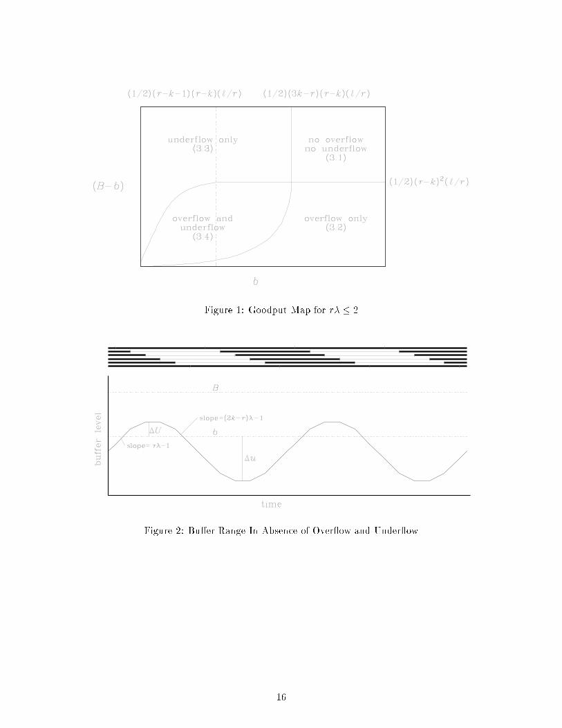
Figure 1: Goodput Map for r� � 2Figure 2: Bu�er Range In Absence of Over ow and Under ow

16

Figure 3: Bu�er Over ow Without Under ow

Figure 4: Goodput Map for r� � 217

0.5

1

1.5

2

2.5

3

3.5

4

4.5

1 1.5 2 2.5 3 3.5 4 4.5 5

Exc

ursi

on /

Pack

et L

engt

h

Overbooking Ratio

simulation: below

analysis: above

simulation: above

analysis: sumsimulation: sum

analysis: sumanalysis: sum

analysis: below 123456789

101112131415

1 1.5 2 2.5 3 3.5 4 4.5 5

Exc

ursi

on /

Pack

et L

engt

h

Overbooking Ratio

simulation: belowanalysis: below

analysis: above

simulation: aboveanalysis: sum

simulation: sum

(a) k = 4 (b) k = 16Figure 5: Normalized excursion above and below the threshold18

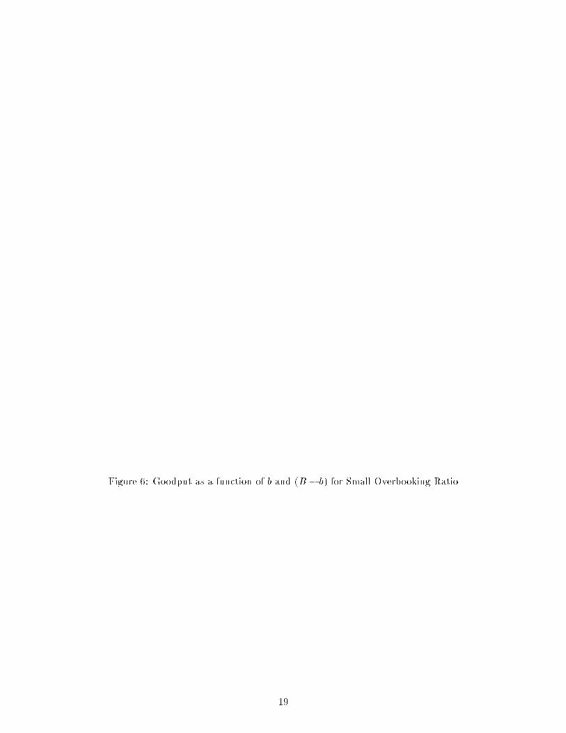
Figure 6: Goodput as a function of b and (B � b) for Small Overbooking Ratio19

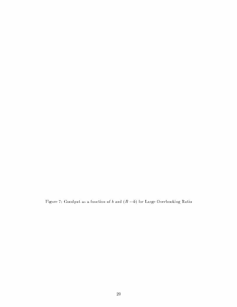
Figure 7: Goodput as a function of b and (B � b) for Large Overbooking Ratio20

0.6

0.65

0.7

0.75

0.8

0.85

0.9

0.95

1

5 10 15 20 25 30

Goo

dput

Overbooking ratio

analysis:worst case analysis:best case

simulation

0.6

0.65

0.7

0.75

0.8

0.85

0.9

0.95

1

5 10 15 20 25 30

Goo

dput

Overbooking ratio

analysis: worst case analysis: best case

simulationFigure 8: Goodput as a function of overbooking ratio (k = 12, ` = 171)max r� for 100% goodput asymptotic goodputb=` b=`.5 1 2 3 4 5 .5 1 2 3 4 51 3 1 1 1 1 1 .67 1 1 1 1 12 1.5 3 1 1 1 1 .80 .67 1 1 1 13 1.23 2.25 4.5 1 1 1 .86 .75 .60 1 1 1k 4 1.16 1.5 3 6 1 1 .89 .80 .67 .57 1 15 1.12 1.3 2.5 3.75 7.5 1 .91 .83 .71 .63 .56 16 1.1 1.23 2.25 3 4.5 9 .92 .86 .75 .67 .60 .558 1.07 1.16 1.5 2.4 3 4 .94 .89 .80 .73 .67 .6210 1.05 1.12 1.3 2.14 2.5 3 .95 .91 .83 .78 .71 .67Figure 9: Extent of Small Overload Region and Asymptotic Throughput21