ON THE OPTIMUM CHECKPOINT SELECTION PROBLEM

ON THE OPTIMUM CHECKPOINT SELECTION PROBLEM*

SAM TOUEG† AND O..

ZALP BABAOGLU†

Abstract. We consider a model of computation consisting of a sequence of n tasks. In the absence of failures,each task i has a known completion time ti . Checkpoints can be placed between any two consecutive tasks. At acheckpoint, the state of the computation is saved on a reliable storage medium. Establishing a checkpoint immedi-ately before task i is known to cost si . This is the time spent in saving the state of the computation. When a failure isdetected, the computation is restarted at the most recent checkpoint. Restarting the computation at checkpoint irequires restoring the state to the previously saved value. The time necessary for this action is given by ri . We derivean O(n3) algorithm to select out of the n − 1 potential checkpoint locations those that result in the smallest expectedtime to complete all the tasks. An O(n2) algorithm is described for the reasonable case where si > s j implies ri ≥ r j .These algorithms are applied to two models of failure. In the first one, each task i has a given probability pi of com-pleting without a failure, i.e., in time ti . Furthermore, failures occur independently and are detected at the end of thetask during which they occur. The second model admits a continuous time failure mode where the failure intervalsare independent and identically distributed random variables drawn from any giv en distribution. In this model, fail-ures are detected immediately. In both models, the algorithm also gives the expected value of the overall completiontime and we show how to derive all the other moments.

Key words. fault-tolerance, checkpoint, rollback-recovery, discrete optimization, renewal process

1. Introduction. A variety of hardware and software techniques have been proposed toincrease the reliability of computing systems that are inherently unreliable. One such soft-ware technique is rollback-recovery. In this scheme, the program is checkpointed from timeto time by saving its state on secondary storage and the computation is restarted at the mostrecent checkpoint after the detection of a failure [6]. Between the times when the failure isdetected and the computation is restarted, the computation must be rolled back to the mostrecent checkpoint by restoring its state to the saved value. Obviously, rollback-recovery is aneffective method only against transient failures. Examples of such failures are temporaryhardware malfunctions, deadlocks due to resource contention, incorrect human interactionswith the computation, and other external factors that can corrupt the computation’s state. Per-sisting failures will block the computation no matter how many times it is rolled back. Theability to detect failures is an essential part of any fault-tolerance method including rollback-recovery. Examples of such failure detection methods are integrity assertion checking [8] andfail-stop processors [10].

In the absence of checkpoints, the computation has to be restated from the beginningwhenever a failure is detected. It is clear that with respect to many objectives such as mini-mum completion time, minimum recovery overhead, maximum throughput, etc., the position-ing of the checkpoints involves certain tradeoffs. A survey of an analytical framework forresolving some of these tradeoffs is presented by Chandy [1]. Young [11] and Chandy et al[3] addressed the problem of finding the checkpoint interval so as to minimize the time lostdue to recovery for a never-ending program subject to failures constituting a Poisson process.Gelenbe and Derochette [5] and Gelenbe [4] have generalized this result to allow the possibil-ity of external requests arriving during the establishment of a checkpoint or rollback-recovery.

* Received by the editors March 9, 1983, and in revised form September 13, 1983. This article was typeset bythe authors at Cornell University on a UNIXTM system. Final copy was produced on November 3, 1983.

† Department of Computer Science, Cornell University, Ithaca, New York 14853. This research was supportedin part by the National Science Foundation under Grants MCS 81-03605 and MCS 82-10356.

These requests are queued and serviced later. Consequently, these results for the optimumcheckpoint intervals with respect to maximizing system availability and minimizing responsetime reflect the dependence on the rate of requests. More recently, Koren et al [7] havederived expressions for optimum parameters in a system employing a combination of instruc-tion retry and rollback-recovery.

In the previous work described above, expressions for the optimum checkpoint intervalwere derived with the assumption that checkpoints could be placed at arbitrary points in theprogram at a cost (as measured in units of time) that is independent of their position. Recallthat establishing a checkpoint implies the saving of the current program state on secondarystorage. As the minimum amount of data required to specify the state of a program can varygreatly over time, it is unrealistic to assume that the time necessary to write it to secondarystorage is a constant. Furthermore, some programs cannot be blocked to create a checkpointduring the execution of certain intervals. The transaction processing periods of a databasesystem are examples of such intervals. Whether due to prohibitive costs or other practicalconsiderations, most computations display only a discrete set of points where checkpoints canbe placed. Informally, we will view these computations as a sequence of tasks such that theprogram state between two consecutive tasks is ‘‘compact’’ (i.e., incurs a reasonable cost tosave). In other words, task boundaries define potential checkpoint locations. Statically, sucha computation can be represented as a directed graph where the vertices denote the tasks andan edge (i, j) exists if and only if task i may be followed by task j in some execution. Thiscomputation model was used by Chandy and Ramamoorthy in the optimum checkpoint selec-tion problem where the objective was to minimize the maximum and expected time spent insaving states [2].

In this paper, we model the execution of a program as a linear sequence of tasks and con-sider the optimum checkpoint selection problem with respect to minimizing the expected totalexecution time of the program subject to failures. In the next section, we introduce the formalprogram model along with the input parameters to the problem. § 3 describes an algorithmbased on dynamic programming that generates the set of checkpoint locations so as to mini-mize the expected completion time. § 4 giv es an improved version of this algorithm that isapplicable when there is a certain relation between the costs for establishing checkpoints andthe costs of rolling back the computation. In § 5, we present two possible failure models towhich the algorithm could be applied. Solutions to some extensions of the original problemare presented in § 6. A discussion of the results concludes the paper.

2. The model of computation. Assume that a computation consists of the sequentialexecution of n tasks where a task may be a program, procedure, function, block, transaction,etc. depending on the environment. For our purposes, any point in the execution where thecomputation is allowed to block and where its state can be represented by a reasonableamount of information can delimit a task. Clearly, the decomposition of the computation intotasks is not unique -- any convenient one will suffice.

Let ti denote the time required to complete task i in the absence of failures. We assumethat these times are deterministic quantities and are known for all of the tasks. The boundarybetween two consecutive tasks i − 1 and i determines the ith candidate checkpoint location.The setup cost, si , is defined to be the time required to establish a checkpoint at location i.This is the time necessary to save the state of the computation on secondary storage as itexists just before task i is executed. After a failure is detected, the state of the computation isrestored to that of the most recent checkpoint. The rollback cost, ri , is defined to be the timerequired to roll back the computation to the checkpoint at location i. After the rollback, the

computation resumes with the execution of task i. We assume that a checkpoint is alwaysestablished just before task 1. Initially, we also assume that the checkpoint setups and roll-backs are failure-free. We relax these last assumptions in § 6.

The optimization problem can now be stated as follows: Given ti , si and ri fori = 1, 2, . . . , n and a suitable failure model, select the subset of the n − 1 potential checkpointlocations such that the resulting expected total completion time (including the checkpointsetup and the rollback-recovery times) for the computation is minimized. The objective func-tion we have selected is a reasonable one for computations that govern time-critical applica-tions such as chemical process control, air traffic control, etc., in the presence of failures.

The following definitions will be used in the subsequent sections. Let [i, j] denote thesequence of tasks i, i + 1, . . . , j where j ≥ i. Note that [1, n] is the entire computation. LetT m

i, j denote the minimum expected execution time for [i, j] over all the possible checkpointselections in [i, j] with m or fewer checkpoints. Clearly, T 0

i, j is the expected execution time of[i, j] without any checkpoints. Among all the checkpoint selections in [i, j] that achieve T m

i, j ,we consider those with the minimum number of checkpoints. These selections are called m-optimal solutions for [i, j], and we denote them by Lm

i, j . Note that a m-optimal solution Lmi, j

for [i, j] contains at most m checkpoints. If Lmi, j contains no checkpoints (i.e., it is the empty

selection of checkpoints), it is written as Lmi, j = < >. If Lm

i, j contains k checkpoints(1 ≤ k ≤ m), we represent it as the ordered sequence of the selected checkpoint locationsLm

i, j = < u1, u2 , . . . , uk >, where i < u1 < u2 < . . . < uk ≤ j. The rightmost checkpoint loca-tion of Lm

i, j = < u1, u2 , . . . , uk > is uk , and the rightmost checkpoint location of Lmi, j = < > is

i . There may be more than one m-optimal solution for [i, j]. From now on, we will consideronly those m-optimal solutions Lm

i, j that satisfy the following additional requirement: EitherLm

i, j = < > or the rightmost checkpoint location of Lmi, j is greater than or equal to the rightmost

checkpoint location of any other m-optimal solution for [i, j]. Henceforth, we reserve thenotation Lm

i, j to denote only those m-optimal solutions for [i, j] that satisfy this additionalrequirement.

The next section describes an algorithm to determine an optimum checkpoint selectionLn−1

1,n and the corresponding minimum expected execution time T n−11,n for a given problem.

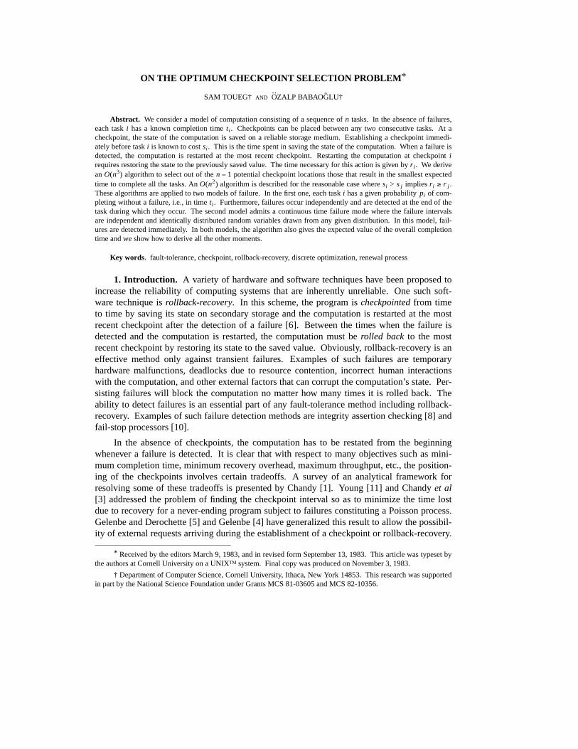
3. The basic algorithm. Consider T k1, j and T k−1

1, j for some k and j such that k ≥ 1 andj ≥ 2. Note that either T k

1, j = T k−11, j or T k

1, j < T k−11, j . Suppose T k

1, j < T k−11, j . In this case, any k-

optimal solution for [1, j] must contain exactly k checkpoints. Let h be the location of therightmost checkpoint of a k-optimal solution for [1, j]. We must have

T k1, j = T k−1

1,h−1 + T 0h, j + sh .

That is, up to k − 1 checkpoints are optimally established in [1, h − 1] and a checkpoint isestablished at location h. No checkpoints are established in [h, j]. Let Lk−1

1,h−1 be any(k − 1)-optimal solution for [1, h − 1]. Then

Lk1, j = Lk−1

1,h−1 || < h >

must be a k-optimal solution [1, j] (the || operator denotes concatenation of sequences, i.e.,< u1, . . . , un > || < v > = < u1, . . . , un, v >).

From these observations, it is clear that we can compute T k1, j and Lk

1, j as follows. Let

T =1<i≤ jMIN (T k−1

1,i−1 + T 0i, j + si)

and let h be the largest index such that T = T k−11,h−1 + T 0

h, j + sh. We must have

for i ← 1 until n dofor j ← i until n do compute T 0

i, j ;

for k ← 1 until n − 1 dobegin

T k1,1 ← T 0

1,1

Lk1,1 ← < >

end;

for k ← 1 until n − 1 do

for j ← n step −1 until 2 do

begin

T ←1<i≤ jMIN (T k−1

1,i−1 + T 0i, j + si)

Let h be the largest minimizing index above

if T < T k−1i, j then do

begin

T k1, j ← T

Lk1, j ← Lk−1

1,h−1 || < h >

end

else do

begin

T k1, j ← T k−1

1, j

Lk1, j ← Lk−1

1, jend;

end;

FIG. 1. Dynamic programming algorithm for computing the optimum checkpoint selection (and thecorresponding expected execution time) for a n-task computation.

T k1, j = MIN(T , T k−1

1, j ). If T k1, j = T k−1

1, j then we have Lk1, j = Lk−1

1, j ; otherwiseLk

1, j = Lk−11,h−1 || < h >.

We just showed that if T 0i, j , T k−1

1,i and Lk−11,i are computed first (for all i’s and j’s such that

1 ≤ i ≤ j), then we can also derive T k1, j and Lk

1, j . This suggests a dynamic programming algo-rithm to compute T n−1

1,n and Ln−11,n . The algorithm is described in detail (in ‘‘Pidgin Algol’’) in

Fig. 1.

Note that the underlying probabilistic failure model does not explicitly appear in thealgorithm. It is implicitly used only during the initialization of the algorithm, when the T 0

i, j’sare computed (for all i’s and j’s such that 1 ≤ i ≤ j ≤ n). Therefore, the same algorithm canbe applied to any underlying failure model such that the T 0

i, j’s can be computed.

If we exclude the computation of the T 0i, j’s, the time complexity of this algorithm is

O(n3). In fact, the inner loop is executed O(n2) times, and the most time-consuming opera-tion in this inner loop is the MIN1<i≤ j operation. Since j = O(n), this operation requires

O(n)-time.

If we assume that the setup costs and the rollback costs are related as described in thenext section, then we can reduce the complexity of the algorithm to O(n2).

We finally note that computing all the T 0i, j’s takes O(n2)-time in the two failure models

that we consider in § 5. Therefore, with these models, the overall complexity of the algo-rithms described in Fig. 1 and in the next section is O(n3) and O(n2), respectively.

4. An improved algorithm for a restricted model. We assume the following relationbetween the setup costs and the rollback costs:

For any two checkpoint locations i and j, if si > s j then ri ≥ r j .

Note that if there is a non-decreasing function f relating all the rollback costs to the setupcosts, i.e., ri = f (si) , then the above relation is satisfied. In particular, it is satisfied if for all iwe have ri = α si + β , for some constant α ≥ 0 and β ≥ 0 . It is also satisfied if all the setupcosts or all the rollback costs are equal.

We further assume that the failure model is such that augmenting any segment cannotdecrease the probability of a failure occurring in that segment. Formally, for all i, j and ksuch that 1 ≤ i ≤ j ≤ k < n, we hav e pi, j ≥ pi,k , where pi, j denotes the probability that nofailures occur during the execution of [i, j]. With these assumptions, we can prove the fol-lowing two theorems.

THEOREM 1. Suppose the m-optimal solutions for [i, j] are such that their rightmostcheckpoint location is k, i ≤ k ≤ j. Then, for any p > j the m-optimal solutions for [i, p] aresuch that their rightmost checkpoint location is some h, h ≥ k.

THEOREM 2. Suppose the m-optimal solutions for [i, j] are such that their rightmostcheckpoint location is k, i ≤ k ≤ j. Then the (m + 1)-optimal solutions for [i, j] are such thattheir rightmost checkpoint location is some h, h ≥ k.

The proofs of these two theorems can be found in the Appendix. From these two theoremswe can immediately derive the following corollary.

COROLLARY. Let a, b, and c be the rightmost checkpoint locations of the (k − 1)-optimalsolutions for [1, j], the k-optimal solutions for [1, j], and the k-optimal solutions for[1, j + 1], respectively (1 < j, k < n). We have a ≤ b ≤ c.

Using this corollary, we can speed up the basic algorithm described in Fig. 1 by a factorof O(n). The main idea is to restrict the range of indexes scanned by the MIN operation in thealgorithm’s inner loop. Suppose we want to compute T k

1, j and we already know some Lk−11, j

and Lk1, j+1. Let lk−1

1, j and lk1, j+1 be the rightmost checkpoint locations of Lk−1

1, j and Lk1, j+1,

respectively. From the corollary, we know that the rightmost checkpoint location i of any k-optimal solution of [1, j] is such that lk−1

1, j ≤ i ≤ lk1, j+1. Therefore, we can compute T k

1, j as fol-lows:

T ←lk−11, j ≤i≤lk

1, j+1

MIN (T k−11,i−1 + T 0

i, j) ,

T ← MIN(T , T k−11, j ) .

Note that, in the algorithm described in Fig. 1, when T k1, j is computed, Lk−1

1, j and Lk1, j+1 have

already been derived in some earlier steps of the algorithm. Therefore, lk−11, j and lk

1, j+1 areknown at that point and they can be used to compute T k

1, j as shown above; Lk1, j is then derived

as in the basic algorithm.

In the basic algorithm of Fig. 1, the range of indexes scanned by the MIN operation tocompute T k

1, j was 1 < i ≤ j. With the algorithm modification that we just described, the range

is lk−11, j ≤ i ≤ lk

1, j+1. We now show that this modification results in an O(n2) algorithm1. Notefirst that a MINa≤i≤b operation in this algorithm takes b − a + 1 steps, i.e., O(b − a) time. Letq, 0 ≤ q ≤ n − 1, be a fixed positive constant. Let T (q) be the following set

T (q) = {T k1, j | 2 ≤ j ≤ n, 1 ≤ k ≤ n − 1, and j − k = q}.

Consider the time taken by all the MIN operations performed while computing all the ele-ments of T (q).

When T 11,q+1 is computed, the range of indexes is 1 ≤ i ≤ l1

1,q+2.

When T 21,q+2 is computed, the range of indexes is l1

1,q+2 ≤ i ≤ l21,q+3.

When T 31,q+3 is computed, the range of indexes is l2

1,q+3 ≤ i ≤ l31,q+4.

...

When T n−q−11,n−1 is computed, the range of indexes is ln−q−2

1,n−1 ≤ i ≤ ln−q−11,n .

When T n−q1,n is computed, the range of indexes is ln−q−1

1,n ≤ i ≤ n.

By summing up the number of computation steps needed by all these MIN operations, we geta total of n + (n − q) steps. Therefore, for any fixed q (0 ≤ q ≤ n − 1), the MIN operationsperformed while computing all the elements of T (q) take a total of O(n) time. By consideringall the n possible values of q, we conclude that the MIN operations performed while comput-ing all the T k

1, j’s such that j − k ≥ 0 take a total of O(n2) time. Similarly, we can show thatthe MIN operations performed while computing all the T k

1, j’s such that j − k < 0 take O(n2)time. Therefore, during the execution of the algorithm the total time taken by MIN is O(n2),and the algorithm’s complexity is also O(n2).

5. Models of failure.

5.1. Discrete case. Our first failure model is discrete where failures occur indepen-dently. In the absence of failures each task i has a known completion time ti and a givenprobability pi of completing without failures (i.e., in time ti). Failures occurring during theexecution of task i are detected only at the end of task i. For example, failure detection couldbe done by checking if an integrity assertion about the state holds at the conclusion of thetask. In this model we also assume that the ti and the rollback times ri are integers.

To use the algorithms of § 3 and § 4 with this failure model, we need to compute all theT 0

i, j’s. Consider a segment [i, j]. Let the random variable Yi, j denote the time required toexecute [i, j] in the presence of failures and no checkpoints. Note that T 0

i, j = E[Yi, j]. Letqt = Prob[Yi, j = t]. The moment generating function Φ(z) = Σ∞t=0 qt z

t of this distribution canbe derived as follows. The execution of [i, j] takes at least ti, j = Σ j

k=i tk units of time. There-fore,

q0 = q1 = . . . = qti, j−1 = 0 .

The execution of [i, j] takes exactly ti, j units of time only if no failures occur. Then we have

1 We exclude the time taken to compute all the T 0i, j’s during the initialization of the algorithm. This time de-

pends on the underlying failure model. We consider two failure models in § 5, and with both models it takes O(n2)time to compute all the T 0

i, j’s.

qti, j= pi pi+1

. . . p j .

The execution of [i, j] takes more than ti, j units of time only if there is at least one failure dur-ing the execution. Consider the first failure that occurs after the computation is started. Byconditioning on all the possible tasks where this failure could occur, we derive the followingrecurrence relation for qt :

qt = (1 − pi)qt−(ti+ri) + pi(1 − pi+1)qt−(ti+ti+1+ri) + . . .

+ pi pi+1. . . p j−1(1 − p j)qt−(ti+ti+1+...+t j+ri)

for all t such that t > ti, j . Multiplying both sides of this equation by zt and summing over allt, t > ti, j , we get

Φ(z) − pi pi+1. . . p j zti+ti+1+...+t j

= (1 − pi) zti+riΦ(z) + pi(1 − pi+1) zti+ti+1+riΦ(z) + . . .

+ pi pi+1. . . p j−1(1 − p j) zti+...+t j+riΦ(z) .

Therefore,

Φ(z) =

pi pi+1. . . p j zti+ti+1+...+t j

1 − (1 − pi)zti+ri − pi(1 − pi+1)zti+ti+1+ri − . . . − pi pi+1. . . p j−1(1 − p j)zti+...+t j+ri

By taking the derivatives of Φ(z) and setting z to one, we can find all the moments of the ran-dom variable Yi, j and, in particular, we can obtain T 0

i, j = E[Yi, j]. It is then easy to verify thatthe following recurrence relation holds

T 0i,i =

ti

pi+ (

1

pi− 1) ri

T 0i, j =

1

p j(T 0

i, j−1 + t j) + (1

p j− 1) ri for all j, j > i .

Using these recurrence relations, we can compute all the T 0i, j’s (for i and j, 1 ≤ i ≤ j ≤ n) in

O(n2)-time.

5.2. Continuous case. Rather than assuming the task executions to constitute indepen-dent Bernoulli trials as we have done in the previous section, let us consider the case wherefailures occur according to a stationary renewal process throughout the computation. In otherwords, the inter-failure times are independent and identically distributed random variables.We assume the existence of a mechanism to detect failures as soon as they occur. As before,when a failure is detected, the computation is rolled back to the most recent checkpoint beforeit can be resumed. We assume that the checkpoint setups and rollbacks constitute renewalpoints.

Let the random variable X denote the time until the next failure after a renewal.F(x) = Prob[X ≤ x] denotes the distribution function of X which is assumed known. Asbefore, let the random variable Yi, j denote the time required to execute [i, j] in the presence offailures and no checkpoints. Let V (t) = Prob[Yi, j ≤ t]. We proceed as follows in order to

derive an expression for this distribution.

As before, ti, j = Σ jk=i tk be the time required to execute [i, j] without any failures.

Clearly, the execution time in the presence of failures cannot be less than this time; that is,V (t) = 0 for t < ti, j . Conditioning on the time until the first failure after a renewal, we have

V (t) =∞

0∫ Prob[Yi, j < t |X = x]dF(x), t ≥ ti, j .

If the length of the first failure-free interval is greater than ti, j , the computation completes inexactly ti, j time units. Consequently, the above equation can be written as

V (t) =

ti, j

0∫ Prob[Yi, j < t |X = x]dF(x) + (1 − F(ti, j)), t ≥ ti, j .

If, however, X = x < ti, j , the computation must be rolled back at least once. Since resumingthe computation after a rollback constitutes a renewal point, the probability that the totalexecution time for [i, j] will be at most t time units after having expended x time units due tothe failure and ri time units for the rollback is simply given by V (t − x − ri). This observationallows us to write V (t) as a renewal equation [9]

V (t) =

ti, j

0∫ V (t − x − ri)dF(x) + (1 − F(ti, j)).

Making the change of variable y = x + ri and the substitutions

z(x) =

0 ,

1 − F(ti, j) ,

x < ti, j ,

x ≥ ti, j

and

G(x) =

0 ,

F(x − ri) ,

F(ti, j) ,

x < ri ,

ri ≤ x ≤ ti, j + ri ,

x > ti, j + ri ,

we obtain

V (t) =t

0∫ V (t − y)dG(y) + z(t), for all t.

Note that the integral represents the convolution of the functions V and g whereg(x) = dG(x)/dx. Taking Laplace transforms yields

V (s) = V (s)g(s) + z(s)

where f (s) = ∫∞

0e−s x f (x)dx denotes the Laplace transform of the function f (x). Finally,

the transform of the distribution we are interested is given by

V (s) =z(s)

1 − g(s)

where z(s) = e−s ti, j (1 − F(ti, j)) / s and g(s) = e−s ri ∫ti, j

0e−s x dF(x).

Whether the inverse transform of V (s) has a closed form solution depends on the natureof F(x). Note that the probability density function of Yi, j , v(t) = dV (t) / dt, has the transform

v(s) = sV (s) =e−s ti, j (1 − F(ti, j))

1 − g(s).

Since the algorithms given in the previous sections need only the values for T 0i, j (by definition,

this is the first moment of Yi, j) for all 1 ≤ i ≤ n and i ≤ j ≤ n, we do not have to obtain theinverse transform of v(s). All of the moments of Yi, j can be obtained by differentiating thetransform of its density. In particular, the first moment is given by

(5.2.1)T 0i, j = E[Yi, j] = −

d

dsv(s)

s=0

= ti, j −

d

dsg(s)|s=0

1 − g(0)

= ti, j +

ri F(ti, j) +

ti, j

0∫ tdF(t)

1 − F(ti, j).

As an example, we will derive an expression for E[Yi, j] in the presence of Poisson fail-ures (i.e., F(x) = 1 − e−λ x and dF(x) = λe−λ x dx where λ is the failure rate). It is important tonote that the above derivation of E[Yi, j] does not rely on the inter-failure times being expo-nentially distributed. We hav e selected the example simply to define one possible form ofF(x). Substituting the expressions for F(x) and dF(x) into equation (5.2.1) and simplifying,we obtain

T 0i, j = E[Yi, j] =

(eλ ti, j − 1)(λri + 1)

λ.

6. Extensions. Up to this point, we have assumed that the checkpoint setups and roll-backs are failure-free. We now discuss how each one of these assumptions can be easilyrelaxed.

Let the checkpoint setups be subject to the same failure model as the normal tasks. Con-sider [i, j] and our computation of T 0

i, j for this segment. Recall that in the algorithm, T 0i, j

denotes the expected execution time of [i, j] giv en that a checkpoint is established at the endof task j. We consider this checkpoint setup to be a new task of length s j+1 which augmentssegment [i, j]. (Obviously, if j = n, the completion of the computation, rather than a check-point, marks the end of the segment. For notational convenience, we define sn+1 = 0.) Theexecution time of the augmented segment without any failures becomes ti, j = Σ j

k=i tk + s j+1 .Following this change, the expected execution time T 0

i, j of the augmented segment can becomputed as shown in § 5. Clearly, since the checkpoint setup costs are now included in theT 0

i, j’s, the minimization step in the algorithm of Fig. 1 becomes

T ←1<i≤ jMIN (T k−1

1,i−1 + T 0i, j) .

Suppose now that checkpoint setups are failure-free but the rollbacks are subject to fail-ures. We can apply the algorithm of Fig. 1 provided that the T 0

i, j’s are computed appropri-ately. For example, in our discrete model of failure, let ρ i be the probability that a rollback tolocation i is failure-free. Proceeding in a similar fashion to § 5.1, we can derive the following

recurrence relation for the new T 0i, j’s:

T 0i,i =

ti

pi+ (

1

pi− 1)

ri

ρ i,

T 0i, j =

1

p j(T 0

i, j−1 + t j) + (1

p j− 1)

ri

ρ ifor all j, j > i.

This extension can be similarly incorporated into the continuous failure model analysis.

Finally, since the necessary modifications for the above extensions to the problem areorthogonal, both of them could be present in the basic algorithm.

7. Discussion and conclusions. We hav e presented an algorithm to select a set of check-point locations out of the n − 1 candidate locations such that the resulting expected executiontime for the computation is minimized. The algorithm can be applied to any failure modelsuch that the expected execution time can be computed for any segment with no checkpoints.The time complexity of this algorithm was shown to be O(n3) where n is the number of tasksmaking up the computation. We also described an O(n2) algorithm for the case that, for all iand j, si > s j implies ri ≥ r j . In most applications, this is a reasonable assumption sincerolling back the state involves loading the same state information which was saved at thecheckpoint.

The objective function we have selected for the optimization problem is the expectedexecution time. For certain time-critical applications, we may be interested in knowing theprobability with which the computation will complete in less than some given time. Notethat, given the optimum checkpoint locations, the computation can be viewed as a sequence ofsegments rather than tasks where each segment is delimited by a checkpoint. The executiontimes for these segments are independent and we have derived their moment generating func-tions (in the two failure models that we considered). The moment generating function for thetotal execution time of the computation is simply the product of the individual segmentmoment generating functions. In principle, this function can be inverted to obtain the distri-bution of the total execution time. Given this distribution, confidence bounds for the totalexecution time can be derived. If inverting the moment generating function is not possible,we can use it to derive the mean, the variance, and any higher moments of the total executiontime (note that the mean is already part of the algorithm’s output). Given these values, we canderive the probability with which the computation completes within a given interval about theknown mean by an application of Chebyshev’s Inequality.

If the static structure of a computation is not simple, its dynamic characterization as asequence of tasks may be difficult to obtain. Given this observation, a generalization of ourwork would represent the static computation as a Directed Acyclic Graph (DAG) where thevertices are tasks and an edge (i, j) denotes a possible execution where task j follows task i.Here we may want to position the checkpoints on this DAG in a way that minimizes the maxi-mum expected execution time over all the possible execution paths. If we augment the DAGby associating probabilities with each edge such that the two tasks connected by the edgeappear in succession with that probability, we can pose the problem of selecting checkpointlocations such that the total expected execution time for the computation is minimized.

Appendix. We introduce some definitions to be used in the following proofs leading tothose of Theorems 1 and 2 of § 4. Consider segment [i, j] for some i ≤ j . Let pi, j be the

probability that no failures occur during the execution of [i, j], α i, j be 1/pi, j and ti, j be theexecution time of [i, j] when no failures occur. Giv en that a failure occurs during the execu-tion of [i, j], li, j denotes the expected time interval from the beginning of task i to the time thefailure is detected.

LEMMA 1. For all i and j such that i ≤ j we have

T 0i, j = ti, j + (α i, j − 1) (li, j + ri) .

For all i, j and k such that i < k ≤ j we have

T 0i, j = α k, j T 0

i,k−1 + tk, j + (α k, j − 1) (lk, j + ri) .

Proof. We present the proofs for the case where the failure times are discrete randomvariables. The continuous case proofs follow simply by replacing the sums with integrals anddiscrete probabilities with density functions.

The first equality can be proven as follows. Let the random variable X denote the timeuntil the first failure is detected after the beginning of [i, j]. Conditioning on this time, wehave

T 0i, j = ti, j ⋅ Prob[X > ti, j] +

x≤ti, j

Σ (x + ri + T 0i, j) ⋅ Prob[X = x].

By definition, pi, j = Prob[X > ti, j]. Consequently,

T 0i, j = ti, j pi, j + (ri + T 0

i, j) (1 − pi, j) +x≤ti, j

Σ xProb[X = x].

Noting that, by definition, li, j = Σx≤ti, jxProb[X = x]/(1 − pi, j), and solving for T 0

i, j we have

pi, j T 0i, j = pi, j ti, j + (1 − pi, j) (li, j + ri) . Dividing both sides by pi, j results in the desired

expression.

To prove the second equality, we condition on the time until the first failure is detectedafter the beginning of [k, j]. Letting X denote this time, we have

T 0i, j = T 0

i,k−1 + tk, j ⋅ Prob[X > tk, j] +x≤tk, j

Σ (x + ri + T 0i, j) ⋅ Prob[X = x].

As before, rewriting this equation in terms of lk, j , and solving for T 0i, j we obtain

pk, j T 0i, j = T 0

i,k−1 + pk, j tk, j + (1 − pk, j) (lk, j + ri) .

Dividing the equation by pk, j completes the proof.

LEMMA 2. For all i, j and k such that i < k ≤ j and α k, j ≠ 1 we have

T 0i,k−1 + T 0

k, j + sk ≤ T 0i, j if and only if sk ≤ (α k, j − 1) (ri + T 0

i,k−1 − rk) .

Furthermore, the equality holds in the left expression if and only if it holds in the right one.

Proof. From Lemma 1 we have

T 0i, j = α k, j T 0

i,k−1 + tk, j + (α k, j − 1) (lk, j + ri)

and

T 0k, j = tk, j + (ak, j − 1) (lk, j + rk) .

Therefore T 0i,k−1 + T 0

k, j + sk ≤ T 0i, j if and only if

T 0i,k−1 + tk, j + (α k, j − 1) (lk, j + rk) + sk ≤α k, j T 0

i,k−1 + tk, j + (α k, j − 1) (lk, j + ri)

This inequality holds if and only if

(α k, j − 1) (lk, j + rk) + sk ≤ (α k, j − 1) (lk, j + ri + T 0i,k−1) .

Since α k, j > 1 , this is satisfied if and only if

lk, j + rk + sk (α k, j − 1)−1 ≤ lk, j + ri + T 0i,k−1 .

This last inequality holds if and only if sk ≤ (α k, j − 1) (ri + T 0i,k−1 − rk) . It is also easy to

check that T 0i,k−1 + T 0

k, j + sk = T 0i, j if and only if sk = (α k, j − 1) (ri + T 0

i,k−1 − rk ) .

LEMMA 3. Suppose the m-optimal solutions for [i, j] are such that their rightmost check-point location is k , i < k ≤ j . Then we have α k, j > 1 and sk < (α k, j − 1) (ri + T 0

i,k−1 − rk) .

Proof. The proof is by induction on m (note that by hypothesis m ≥ 1).

Suppose m = 1 . By hypothesis we have

(L3.1)T 1i, j = T 0

i,k−1 + T 0k, j + sk < T 0

i, j .

If we show that α k, j ≠ 1 then Lemma 3 follows directly from Lemma 2. Suppose α k, j = 1 .From Lemma 1 we have T 0

i, j = T 0i,k−1 + tk, j and T 0

k, j = tk, j . Therefore, T 0i, j = T 0

i,k−1 + T 0k, j

and this contradicts (L3.1). So α k, j > 1 and Lemma 3 follows.

Now assume Lemma 3 holds for all m , 1 ≤ m < r , for some r > 1 . We show that itmust also hold for m = r . Suppose the r-optimal solutions for [i, j] are such that their right-most checkpoint location is k , i < k ≤ j . Let Lr−1

i,k−1 be a (r − 1)-optimal solution for[i, k − 1] . We consider Lr

i, j = Lr−1i,k−1 || < k > . Note that this must be a r-optimal solution for

[i, j] . Let h be the rightmost checkpoint location of Lr−1i,k−1 . We hav e i ≤ h < k ≤ j .

Assume first that i < h . By induction hypothesis we havesh < (α h,k−1 − 1) (ri + T 0

i,h−1 − rh) , and α h,k−1 > 1 . Note that sh ≥ 0 , and therefore

(L3.2)rh < ri + T 0i,h−1 .

Since L1h, j = < k > is a 1-optimal solution for [h, j] then, by induction hypothesis, we have

α k, j > 1 and sk < (α k, j − 1) (rh + T 0h,k−1 − rk) . Suppose, for contradiction, that

sk ≥ (α k, j − 1) (ri + T 0i,k−1 − rk) . Combining the last two inequalities we have

ri + T 0i,k−1 < rh + T 0

h,k−1 . From Lemma 1 we have

ri + [α h,k−1 T 0i,h−1 + th,k−1 + (α h,k−1 − 1) (lh,k−1 + ri) ]

< rh + [ th,k−1 + (α h,k−1 − 1) (lh,k−1 + rh) ] .

So (ri + T 0i,h−1)α h,k−1 < rh α h,k−1 , and ri + T 0

i,h−1 < rh contradicting (L3.2). Therefore wemust have sk < (α k, j − 1) (ri + T 0

i,k−1 − rk) .

Suppose now that i = h . In this case it is clear that Lr−1i,k−1 = < > and Lr

i, j = < k > , there-fore L1

i, j = < k > , i.e., < k > is the 1-optimal checkpoint selection for [i, j]. Then, by induc-tion hypothesis, we have α k, j > 1 and sk < (α k, j − 1) (ri + T 0

i,k−1 − rk).

LEMMA 4. Suppose the m-optimal solutions for [i, j] are such that the rightmost check-point location is k , i < k ≤ j . Then for all h , i < h < k , we have

sk − sh ≤ (α k, j − 1) (rh + T 0h,k−1 − rk) .

Proof. We prove the lemma by induction on m (note that by hypothesis m ≥ 1).

Assume first that m = 1 . Suppose, for contradiction, that for some h , i < h < k , wehave

(L4.1)sk − sh > (α k, j − 1) (rh + T 0h,k−1 − rk).

From Lemma 3 we have sk < (α k, j − 1) (ri + T 0i,k−1 − rk) , and α k, j > 1 . Therefore,

rh + T 0h,k−1 < ri + T 0

i,k−1 , and from Lemma 1 we have

rh + [ th,k−1 + (α h,k−1 − 1) (lh,k−1 + rh) ]

< ri + [α h,k−1 T 0i,h−1 + th,k−1 + (α h,k−1 − 1) (lh,k−1 + ri) ]

so, α h,k−1 rh < α h,k−1 (ri + T 0i,h−1) , and

(L4.2)rh < ri + T 0i,h−1.

Since < k > is the 1-optimal solution for [i, j] we hav e

T 1i, j = T 0

i,k−1 + T 0k, j + sk ≤ T 0

i,h−1 + T 0h, j + sh

and therefore T 0i,k−1 − T 0

i,h−1 + sk ≤ T 0h, j − T 0

k, j + sh . We define ∆1 = T 0i,k−1 − T 0

i,h−1 and∆2 = T 0

h, j − T 0k, j , and we write the last inequality as

(L4.3)∆1 + sk ≤ ∆2 + sh .

Applying Lemma 1 we have

∆1 = [α h,k−1 T 0i,h−1 + th,k−1 + (α h,k−1 − 1) (lh,k−1 + ri) ] − T 0

i,h−1

so

∆1 = th,k−1 + (α h,k−1 − 1) (lh,k−1 + ri + T 0i,h−1) .

We also have

∆2 = [α k, jT0h,k−1 + tk, j + (α k, j − 1) (lk, j + rh) ] − [ tk, j + (α k, j − 1) (lk, j + rk) ]

and therefore

∆2 = α k, jT0h,k−1 + (α k, j − 1) (rh − rk) .

From (L4.1) we have rh − rk < −T 0h,k−1 + (sk − sh) (α k, j − 1)−1 . Therefore,

∆2 < α k, j T 0h,k−1 − (α k, j − 1) T 0

h,k−1 + sk − sh , that is

(L4.4)∆2 < T 0h,k−1 + sk − sh .

From (L4.3) and (L4.4) we obtain

(L4.5)∆1 < T 0h,k−1 ,

that is, th,k−1 + (α h,k−1 − 1) (lh,k−1 + ri + T 0i,h−1) < T 0

h,k−1 . By Lemma 1 we have

th,k−1 + (α h,k−1 − 1) (lh,k−1 + ri + T 0i,h−1) < th,k−1 + (α h,k−1 − 1) (lh,k−1 + rh)

so (α h,k−1 − 1) (ri + T 0i,h−1) < (α h,k−1 − 1) rh . Suppose α h,k−1 = 1 . Then ∆1 = th,k−1 and

T 0h,k−1 = th,k−1 , a contradiction to (L4.5). So we must have α h,k−1 > 1 and ri + T 0

i,h−1 < rh .But this contradicts (L4.2) and therefore sk − sh ≤ (α k, j − 1) (rh + T 0

h,k−1 − rk) for all h,i < h < k .

Now assume the lemma holds for all m, 1 ≤ m < r, for some r > 1. We show that it mustalso hold for m = r . Suppose the r-optimal solutions for [i, j] are such that their rightmostcheckpoint location is k, i < k ≤ j . Let Lr−1

i,k−1 be a (r − 1)-optimal solution for [i, k − 1] . Weconsider Lr

i, j = Lr−1i,k−1 || < k > . Note that this must be a r-optimal solution for [i, j] . Let p

be the location of the rightmost checkpoint of Lr−1i,k−1 . Note that i ≤ p < k ≤ j .

Assume first that i < p . Consider some h such that i < h < k . There are two possiblecases, either p < h or h ≤ p . We show that in both casessk − sh ≤ (α k, j − 1) (rh + T 0

h,k−1 − rk) .

(i) Suppose i < p < h < k ≤ j . Since k must be the (rightmost) checkpoint location of the1-optimal solution for [p, j] then, by induction hypothesis, we havesk − sh ≤ (α k, j − 1) (rh + T 0

h,k−1 − rk) .

(ii) We now consider h such that i < h ≤ p < k ≤ j . Suppose, for contradiction, thatsk − sh > (α k, j − 1) (rh + T 0

h,k−1 − rk) . Since L1p, j = < k > is a 1-optimal solution for [p, j]

then, by Lemma 3, we have sk < (α k, j − 1) (r p + T 0p,k−1 − rk) , and α k, j > 1 . Combining the

last two inequalities we have rh + T 0h,k−1 < r p + T 0

p,k−1 . Therefore h ≠ p (i.e., h < p), andfrom Lemma 1 we have

rh + [α p,k−1 T 0h,p−1 + t p,k−1 + (α p,k−1 − 1) (l p,k−1 + rh) ]

< r p + [ t p,k−1 + (α p,k−1 − 1)(l p,k−1 + r p) ] .

By simplifying we obtain

(L4.6)rh + T 0h,p−1 < r p .

Since the rightmost checkpoint location of the (r − 1)-optimal solutions for [i, k − 1] is p,and i < h < p ≤ k − 1 , then, by induction hypothesis, we have

(L4.7)s p − sh ≤ (α p,k−1 − 1) (rh + T 0h,p−1 − r p) .

From Lemma 3 we also have α p,k−1 > 1 . From (L4.6) and (L4.7) we obtain s p − sh < 0 .From our assumption about checkpointing costs either s p = sh, a contradiction, or r p ≤ rh

which contradicts (L4.6). So we must have sk − sh ≤ (α k, j − 1) (rh + T 0h,k−1 − rk) .

Suppose now that i = p . In this case it is clear that Lr−1i,k−1 = < > and Lr

i, j = < k >, andtherefore L1

i, j = < k > , i.e., < k > is the 1-optimal checkpoint selection for [i, j]. Then, byinduction hypothesis, we have sk − sh ≤ (α k, j − 1) (rh + T 0

h,k−1 − rk) , for all h, i ≤ h < k .

LEMMA 5. Suppose the m-optimal solutions for [i, j] are such that their rightmost check-point location is k, i ≤ k ≤ j . Consider h and p such that i ≤ h ≤ k ≤ j ≤ p . If i = h orsh ≤ sk then we have T 0

k,p − T 0k, j ≤ T 0

h,p − T 0h, j .

Proof. The result is obvious for i = k, or h = k, or j = p. Otherwise, suppose that forcontradiction

(L5.1)T 0k,p − T 0

k, j > T 0h,p − T 0

h, j

for some i ≤ h < k ≤ j < p such that i = h or sh ≤ sk . From Lemma 1 we have

T 0k,p = α j+1,p T 0

k, j + t j+1,p + (α j+1,p − 1) (l j+1,p + rk)

and therefore

(L5.2)T 0k,p − T 0

k, j = t j+1,p + (α j+1,p − 1) (T 0k, j + l j+1,p + rk) .

Similarly we have

(L5.3)T 0h,p − T 0

h, j = t j+1,p + (α j+1,p − 1) (T 0h, j + l j+1,p + rh) .

From (L5.1), (L5.2) and (L5.3) we have

(α j+1,p − 1) (T 0k, j + l j+1,p + rk) > (α j+1,p − 1) (T 0

h, j + l j+1,p + rh) .

Suppose α j+1,p = 1 . In this case, from (L5.2) and (L5.3) we haveT 0

k,p − T 0k, j = T 0

h,p − T 0h, j = t j+1,p which contradicts (L5.1). Therefore α j+1,p > 1 , and we have

(L5.4)rk + T 0k, j > rh + T 0

h, j .

Note that h < k ≤ j and by applying Lemma 1 we derive

rk + [ tk, j + (α k, j − 1) (lk, j + rk) ] > rh + [α k, j T 0h,k−1 + tk, j + (α k, j − 1) (lk, j + rh) ] .

Then we have α k, j rk > α k, j (rh + T 0h,k−1) and

(L5.5)rk > rh + T 0h,k−1 .

From Lemma 3, we have sk < (α k, j − 1) (ri + T 0i,k−1 − rk) , and α k, j > 1 , therefore

(L5.6)rk < ri + T 0i,k−1 .

If i = h then (L5.6) contradicts (L5.5). Suppose i < h . From Lemma 4, we havesk − sh ≤ (α k, j − 1) (rh + T 0

h,k−1 − rk) . Therefore, if sh ≤ sk , then rk ≤ rh + T 0h,k−1 which

also contradicts (L5.5). Then neither i = h nor sh ≤ sk and the proof is complete.

LEMMA 6. If i ≤ h ≤ k ≤ j and rk ≤ rh then T 0k, j ≤ T 0

h, j .

Proof. The lemma is obvious for h = k . We now assume i ≤ h < k ≤ j . From Lemma1 we hav e

T 0h, j = α k, j T 0

h,k−1 + tk, j + (α k, j − 1) (lk, j + rh)

and T 0k, j = tk, j + (α k, j − 1) (lk, j + rk) . Therefore we have

T 0h, j − T 0

k, j = α k, j T 0h,k−1 + (α k, j − 1) (rh − rk)

and since rk ≤ rh then T 0h, j − T 0

k, j ≥ 0 .

LEMMA 7. If i ≤ h ≤ k ≤ j ≤ p and rk ≤ rh then T 0h, j − T 0

k, j ≤ T 0h,p − T 0

k,p .

Proof. The lemma is obvious if h = k or j = p . We now assume thati ≤ h < k ≤ j < p . In the proof of Lemma 6 we showed that

T 0h, j − T 0

k, j = α k, j T 0h,k−1 + (α k, j − 1) (rh − rk)

and similarly we have

T 0h,p − T 0

k,p = α k,p T 0h,k−1 + (α k,p − 1) (rh − rk) .

Since p > j it is clear that α k,p ≥ α k, j . By hypothesis we also have rh − rk ≥ 0 and thereforeT 0

h, j − T 0k, j ≤ T 0

h,p − T 0k,p .

THEOREM 1. Suppose the m-optimal solutions for [i, j] are such that their rightmostcheckpoint location is k, i ≤ k ≤ j . Then for any p > j the m-optimal solutions for [i, p] aresuch that their rightmost checkpoint location is some h, h ≥ k .

Proof. If i = k, the theorem is obvious. Assume i < k and therefore m ≥ 1 . Suppose,for contradiction, that the rightmost checkpoint location of the m-optimal solutions for [i, p]is h, i ≤ h < k .

Assume first that i < h . By hypothesis we must have

(T1.1)T m−1i,k−1 + T 0

k, j + sk ≤ T m−1i,h−1 + T 0

h, j + sh .

From our definition of h we also have

(T1.2)T m−1i,k−1 + T 0

k,p + sk ≥ T m−1i,h−1 + T 0

h,p + sh .

Suppose equality holds in (T1.1). Then the (m − 1)-optimal solutions for [i, h − 1] cannotinclude fewer checkpoints than the (m − 1)-optimal solutions for [i, k − 1] . Therefore equal-ity cannot also hold in (T1.2), otherwise k would be the rightmost checkpoint location of them-optimal solutions for [i, p] contradicting our definition of h. So equality cannot holdsimultaneously in (T1.1) and in (T1.2). Then, subtracting (T1.1) from (T1.2) we obtain

(T1.3)T 0k,p − T 0

k, j > T 0h,p − T 0

h, j .

If sh ≤ sk then (T1.3) contradicts Lemma 5; therefore sk < sh . From our assumption aboutcheckpointing costs we have rk ≤ rh . Then, from Lemma 6, we also have T 0

k, j ≤ T 0h, j , so

(T1.4)rk + T 0k, j ≤ rh + T 0

h, j .

However, in the proof of Lemma 5 we showed that (T1.3) implies rk + T 0k, j > rh + T 0

h, j whichcontradicts (T1.4).

Suppose now that i = h , i.e., the m-optimal solutions for [i, p] contain no checkpoints(Lm

i,p = < > ). In this case we must have

(T1.5)T m−1i,k−1 + T 0

k, j + sk < T 0i, j .

Since Lmi,p = < > then

(T1.6)T m−1i,k−1 + T 0

k,p + sk ≥ T 0i,p .

Subtracting (T1.5) from (T1.6) we obtain (T1.3). From (T1.3) we can also derive a contradic-tion exactly as before, and the proof is complete.

THEOREM 2. Suppose the m-optimal solutions for [i, j] are such that their rightmostcheckpoint location is k, i ≤ k ≤ j . Then the (m + 1)-optimal solutions for [i, j] are such thattheir rightmost checkpoint location is some h, h ≥ k .

Proof. If i = k, the theorem is obvious. Assume i < k and therefore m ≥ 1 . IfT m+1

i, j = T mi, j then m-optimal solutions for [i, j] are also (m + 1)-optimal solutions for [i, j] and

the theorem clearly holds. We now assume T m+1i, j < T m

i, j . Note that in this case (m + 1)-opti-mal solutions for [i, j] hav e exactly m + 1 checkpoints. Let g be the number of checkpoints inthe m-optimal solutions for [i, j]. Note that 1 ≤ g ≤ m . We form a particular m-optimal solu-tion Lm

i, j = < ug, ug−1 , . . . , u1 > for [i, j] as follows. Let u1 be the rightmost checkpoint loca-tion of the m-optimal solutions for [i, j] , let u2 be the rightmost checkpoint location of the(m − 1)-optimal solutions for [i, u1 − 1] , . . . , and let ug be the rightmost checkpoint locationof the [(m + 1) − g]-optimal solutions for [i, ug−1 − 1] . Note that with this construction< ug, ug−1 , . . . , u f > is a [(m + 1) − f ]-optimal solution for [i, u f −1 − 1] , for all f ,2 ≤ f ≤ g . By hypothesis we have u1 = k . We also form in a similar way a particular(m + 1)-solution Lm+1

i, j = < vm+1, vm , . . . , v1 > for [i, j] . We define v1 = h . Suppose, forcontradiction, that h < k (i.e., v1 < u1). There are two possible cases. We show that each oneleads to a contradiction.

I. Suppose first that vm ≤ ug . Note that vm+1 < vm and therefore vm+1 < ug . SinceLm

i, j = < ug, ug−1 , . . . , u1 > is a m-optimal solution for [i, j] we hav e

T mi, j = T 0

i,ug − 1 +1

l=g−1Σ T 0

ul+1,ul − 1 + T 0u1, j +

1

l=gΣ sul

and

T mi, j ≤ T 0

i,vm − 1 +1

l=m−1Σ T 0

vl+1,vl − 1 + T 0v1, j +

1

l=mΣ svl

where the indexes of the summations scan the segments from left to right, and the summationb

l=aΣ ... is defined to be zero if a < b .

Therefore,

(T2.1)T 0i,ug − 1 − T 0

i,vm − 1 + F ≤ 0

where

F =1

l=g−1Σ T 0

ul+1,ul − 1 −1

l=m−1Σ T 0

vl+1,vl − 1 + T 0u1, j − T 0

v1, j +1

l=gΣ sul

−1

l=mΣ svl

.

Since Lm+1i, j = < vm+1, vm , . . . , v1 > is a (m + 1)-optimal solution for [i, j] we hav e

T m+1i, j = T 0

i,vm+1 − 1 + T 0vm+1,vm − 1 +

1

l=m−1Σ T 0

vl+1,vl − 1 + T 0v1, j + svm+1

+1

l=mΣ svl

.

(T2.2)

Note that if the < vm+1, ug, ug−1 , . . . , u1 > selection of checkpoints achieved the time T m+1i, j

(or less) this would contradict our assumption that the rightmost checkpoint location of the(m + 1)-optimal solutions for [i, j] is v1 < u1 . Therefore we must have

T m+1i, j < T 0

i,vm+1 − 1 + T 0vm+1,ug − 1 +

1

l=g−1Σ T 0

ul+1,ul − 1 + T 0u1, j + svm+1

+1

l=gΣ sul

.

(T2.3)

Subtracting (T2.2) from (T2.3) we get

(T2.4)0 < T 0vm+1,ug − 1 − T 0

vm+1,vm − 1 + F .

From (T2.1) and (T2.4) we have

(T2.5)T 0vm+1,ug − 1 − T 0

vm+1,vm − 1 > T 0i,ug − 1 − T 0

i,vm − 1 .

Note that i < vm+1 ≤ vm − 1 ≤ ug − 1 and < vm+1 > is the 1-optimal solution for [i, vm − 1] .By Lemma 5 we have

T 0vm+1,ug − 1 − T 0

vm+1,vm − 1 ≤ T 0i,ug − 1 − T 0

i,vm − 1

which contradicts (T2.5).

II. Suppose now that vm > ug . Let k be the minimum r such that v1 ≤ u1 , v2 ≤ u2 , . . . ,vr−1 ≤ ur−1 , and vr > ur . Note that such k exists because vm > ug (and therefore vg > ug ).There are two possible cases.

(i) Suppose vk+1 ≤ uk . In this case we have vk+1 ≤ uk < vk < vk−1 ≤ uk−1 . SinceLm

i, j = < ug , . . . , u1 > is a m-optimal solution for [i, j] we hav e

T mi, j =T 0

i,ug − 1 +k

l=g−1Σ T 0

ul+1,ul − 1 + T 0uk ,uk−1 − 1 +

1

l=k−2Σ T 0

ul+1,ul − 1 + T 0u1, j +

1

l=gΣ sul

.

(T2.6)

The checkpoint selection < ug , . . . , uk , vk−1 , . . . , v1 > cannot achieve a smaller time than T mi, j

for [i, j] . Therefore we have

(T2.7)T mi, j ≤ T (u, v)

where T (u, v) is defined as

T (u, v) = T 0i,ug − 1 +

k

l=g−1Σ T 0

ul+1,ul − 1 +T 0uk ,vk−1 − 1

+1

l=k−2Σ T 0

vl+1,vl − 1 +T 0v1, j +

k

l=gΣ sul

+1

l=k−1Σ svl

.

From (T2.6) and (T2.7) we have

(T2.8)T 0uk ,uk−1 − 1 − T 0

uk ,vk−1 − 1 + G ≤ 0

where

G =1

l=k−2Σ (T 0

ul+1,ul − 1 − T 0vl+1,vl − 1 ) + T 0

u1, j − T 0v1, j +

1

l=k−1Σ (sul

− svl) .

Since Lm+1i, j = < vm+1 , . . . , vk , vk−1 , . . . , v1 > is a (m + 1)-optimal solution for [i, j] we hav e

T m+1i, j =T 0

i,vm+1 − 1 +k

l=mΣ T 0

vl+1,vl − 1 +T 0vk ,vk−1 − 1 +

1

l=k−2Σ T 0

vl+1,vl − 1 +T 0v1, j +

1

l=m+1Σ svl

.

(T2.9)Since with u1 > v1 then the < vm+1 , . . . , vk , uk−1 , . . . , u1 > checkpoint selection cannotachieve the time T m+1

i, j (or less) for [i, j] without contradicting the optimality of Lm+1i, j .

Therefore we have

(T2.10)T m+1i, j < T (v, u)

where T (v, u) is defined as

T (v, u) = T 0i,vm+1 − 1 +

k

l=mΣ T 0

vl+1,vl − 1 +T 0vk ,uk−1 − 1

+1

l=k−2Σ T 0

ul+1,ul − 1 +T 0u1, j +

k

l=m+1Σ svl

+1

l=k−1Σ sul

.

Subtracting (T2.9) from (T2.10) we have

(T2.11)0 < T 0vk ,uk−1 − 1 − T 0

vk ,vk−1 − 1 + G .

From (T2.8) and (T2.11) we have

(T2.12)T 0vk ,uk−1 − 1 − T 0

vk ,vk−1 − 1 > T 0uk ,uk−1 − 1 − T 0

uk ,vk−1 − 1 .

Note that we have vk+1 ≤ uk < vk ≤ vk−1 − 1 ≤ uk−1 − 1 and < vk > is the 1-optimal solutionfor [vk+1, vk−1 − 1] . By Lemma 5 we know that if svk

≥ sukthen

(T2.13)T 0vk ,uk−1 − 1 − T 0

vk ,vk−1 − 1 ≤ T 0uk ,uk−1 − 1 − T 0

uk ,vk−1 − 1

which contradicts (T2.12); therefore svk< suk

. From our assumption about checkpointingcosts we have rvk

≤ ruk.

From (T2.7) and (T2.10) we have T (u, v) − T m+1i, j > T m

i, j − T (v, u) , that is

(T2.14)T 0uk ,vk−1 − 1 − T 0

vk ,vk−1 − 1 > T 0uk ,uk−1 − 1 − T 0

vk ,uk−1 − 1 .

But since vk+1 ≤ uk < vk ≤ vk−1 − 1 ≤ uk−1 − 1 , and rvk≤ ruk

then we can apply Lemma 7and obtain T 0

uk ,vk−1 − 1 − T 0vk ,vk−1 − 1 ≤ T 0

uk ,uk−1 − 1 − T 0vk ,uk−1 − 1 . This contradicts (T2.14) and there-

fore we cannot have vk+1 ≤ uk .

(ii) Suppose vk+1 > uk . In this case we have uk < vk+1 < vk < vk−1 ≤ uk−1 . We show that thisis not possible. Observe that < ug , . . . , uk > is a [(m + 1) − k]-optimal solution for[i, uk−1 − 1]; its rightmost checkpoint location is uk , uk < vk+1 . We also note that< vm+1 , . . . , vk+1 > is a [(m + 1) − k]-optimal solution for [i, vk − 1] . Since uk−1 − 1 > vk − 1then, by Theorem 1, the rightmost checkpoint location of the [(m + 1) − k]-optimal solutionsfor [i, uk−1 − 1] is some u such that u ≥ vk+1 . Since uk < vk+1, this contradicts the optimalityof < ug , . . . , uk > for [i, uk−1 − 1] , and the proof is complete.

REFERENCES

[1] K. M. CHANDY, A survey of analytic models of rollback and recovery strategies, Com-puter, 5 (1975), pp. 40-47.

[2] K. M. CHANDY AND C.V. RAMAMOORTHY, Rollback and recovery strategies for computerprograms, IEEE Trans. on Comput., 6 (1972), pp. 546-556.

[3] K. M. CHANDY, J. C. BRO WNE, C. W. DISSLY AND W. R. UHRIG, Analytic models for roll-back and recovery strategies in data base systems, IEEE Trans. on Soft. Engr., 1(1975), pp. 100-110.

[4] E. GELENBE, On the optimum checkpoint interval, J. Assoc. Comput. Mach., 2 (1979),pp. 259-270.

[5] E. GELENBE AND D. DEROCHETTE, Performance of rollback recovery systems under inter-mittent failures, Comm. Assoc. Comput. Mach., 6 (1978), pp. 493-499.

[6] J. GRAY, P. MCJONES, M. BLASGEN, B. LINSAY, R. LORIE, T. PRICE, F. PUTZOLU AND I.TRAIGER, The recovery manager of the System R database manager, Comput. Surveys,2 (1981), pp. 223-242.

[7] I. KOREN, Z. KOREN AND S. SU, Analysis of a recovery procedure, Tech. Report, Tech-nion-Israel Institute of Technology, (1983). To appear in IEEE Trans. on Comput.

[8] B. RANDELL, P. LEE AND P. TRELEAVEN, Reliability issues in computing system design,Comput. Surveys, 2 (1978), pp. 123-166.

[9] S. M. ROSS, Applied probability models with optimization applications, Holden-Day,San Francisco, CA, 1970.

[10] R. D. SCHLICHTING, AND F.B. SCHNEIDER, Fail-stop processors: an approach to designingfault-tolerant computing systems, ACM Trans. on Computer Systems, 3 (1983), pp.222-238.

[11] J. W. YOUNG, A first order approximation to the optimum checkpoint interval, Comm.Assoc. Comput. Mach., 9 (1974), pp. 530-531.