On the Numerical Computation of Enzyme Kinetic Parameters

Article Biomath Communications 1 (2014)

Biomath Communications

www.biomathforum.org/biomath/index.php/conference

On the Numerical Computation of EnzymeKinetic Parameters 1

Stanko Dimitrov1, Gergana Velikova1, Venko Beschkov2, SvetoslavMarkov3

1 University of Sofia, Faculty of Mathematics and Informatics,[email protected]

2 Institute of Chemical Engineering, Bulgarian Academy of Sciences3 Institute of Mathematics and Informatics, Bulgarian Academy of

Sciences

Abstract

We consider the enzyme kinetic reaction scheme originally pro-posed by V. Henri of single enzyme-substrate dynamics where twofractions of the enzyme—free and bound—are involved. Henri’s schemeinvolves four concentrations and three rate constants and via themass action law it is translated into a system of four ODEs. In twocase studies we demonstrate how the rate constants can be computedwhenever time course experimental data are available. The obtainedresults are compared with analogous results implied by the classicalMichaelis-Menten model. Our approach focuses on the uncertaintiesin the experimental data, as well as on the use of contemporary com-putational tools such as CAS Mathematica.

Keywords: enzyme kinetics, biomass-substrate-product dynamics, computa-tion of rate constants, ODE systems, uncertainties, interval methods, veri-fication methods, CAS Mathematica

1 Citation: S. Dimitrov, G. Velikova, V. Beshkov, S. Markov, On the NumericalComputation of Enzyme Kinetic Parameters. Biomath Communications 1/2 (2014)http://dx.doi.org/10.11145/j.bmc.2015.02.201

1

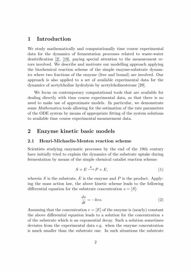
1 Introduction

We study mathematically and computationally time course experimentaldata for the dynamics of fermentation processes related to waste-waterdenitrification [2], [19], paying special attention to the measurement er-rors involved. We describe and motivate our modelling approach applyingthe biochemical reaction scheme of the simple enzyme-substrate dynam-ics where two fractions of the enzyme (free and bound) are involved. Ourapproach is also applied to a set of available experimental data for thedynamics of acetylcholine hydrolysis by acetylcholinesterase [29].

We focus on contemporary computational tools that are available fordealing directly with time course experimental data, so that there is noneed to make use of approximate models. In particular, we demonstratesome Mathematica tools allowing for the estimation of the rate parametersof the ODE system by means of appropriate fitting of the system solutionsto available time course experimental measurement data.

2 Enzyme kinetic basic models

2.1 Henri-Michaelis-Menten reaction scheme

Scientists studying enzymatic processes by the end of the 19th centuryhave initially tried to explain the dynamics of the substrate uptake duringfermentation by means of the simple chemical catalist reaction scheme:

S + Ek−→P + E, (1)

wherein S is the substrate, E is the enzyme and P is the product. Apply-ing the mass action law, the above kinetic scheme leads to the followingdifferential equation for the substrate concentration s = [S]:

ds

dt= −kes. (2)

Assuming that the concentration e = [E] of the enzyme is (nearly) constantthe above differential equation leads to a solution for the concentration sof the substrate which is an exponential decay. Such a solution sometimesdeviates from the experimental data e.g. when the enzyme concentrationis much smaller than the substrate one. In such situations the substrate

2

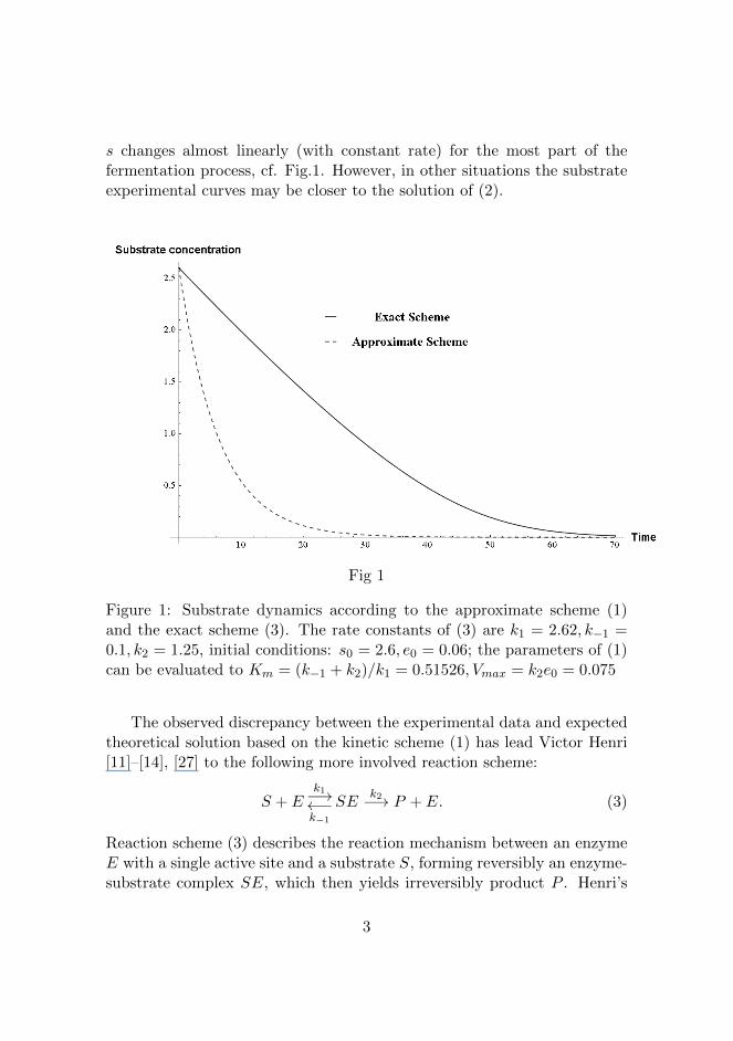
s changes almost linearly (with constant rate) for the most part of thefermentation process, cf. Fig.1. However, in other situations the substrateexperimental curves may be closer to the solution of (2).

Fig 1

Figure 1: Substrate dynamics according to the approximate scheme (1)and the exact scheme (3). The rate constants of (3) are k1 = 2.62, k−1 =0.1, k2 = 1.25, initial conditions: s0 = 2.6, e0 = 0.06; the parameters of (1)can be evaluated to Km = (k−1 + k2)/k1 = 0.51526, Vmax = k2e0 = 0.075

The observed discrepancy between the experimental data and expectedtheoretical solution based on the kinetic scheme (1) has lead Victor Henri[11]–[14], [27] to the following more involved reaction scheme:

S + Ek1−→←−k−1

SEk2−→ P + E. (3)

Reaction scheme (3) describes the reaction mechanism between an enzymeE with a single active site and a substrate S, forming reversibly an enzyme-substrate complex SE, which then yields irreversibly product P . Henri’s

3

reaction scheme (3) says that during the transition of the substrate S intoproduct P the enzyme E bounds the substrate into a complex SE havingdifferent properties than the free enzyme and thus necessarily consideredas a separate substance.

2.2 Michaelis-Menten equation

Applying the mass action law to Henri’s reaction scheme (3) one obtainsa general dynamical system, which under the so-called quasi-steady-stateassumption [18], [20], [21], [22] leads to the following reaction equation forthe substrate rate ds/dt:

ds

dt= − Vmaxs

Km + s. (4)

The quasi-steady-state assumption is applied whenever the ratio [E]/[S] issmall so that the fermentation process has a considerably long time intervalduring which the concentration [ES] of the bound enzyme is constant [28].

In their seminal paper Michaelis and Menten discussed in detail Henri’sreaction scheme and equation (4) which became known as the Michaelis-Menten equation (MM-equation) [17], see also [15]. In addition Michaelisand Menten discussed at length the meaning of the rate constants in Henri’sreaction scheme and proposed a protocol for the practical calculation of theconstant Km in (4). The constant Km is known as Michaelis constant (forthe history of these investigations see [5], [26].

The MM-equation (4) can be written in the form

ds

dt= − Vmaxs

Km + s= − Vmax

Km/s+ 1,

showing that for large values of s the right-hand side is close to the constant−Vmax; hence the uptake rate is almost constant (zero-order kinetic).

Michaelis-Menten equation (4) is simple, can be easily used by non-mathematicians; the protocol for calculation of the Michaelis constant Km

suggested in [17] has been later modified [16] and is still used in practice.

However, the MM-equation (4) gives good approximation only undercertain conditions [9], [28]. Thus the condition e0 << s0 assures goodapproximation and is ubiquitous for many fermentation processes, but is

4

not present e.g. in living cells [25]. Next we propose methods and tools forthe computation of the Michaelis constant based on the general system ofdifferential equations induced by Henri’s reaction scheme (3).

2.3 Enzyme kinetics induced by Henri’s reaction scheme

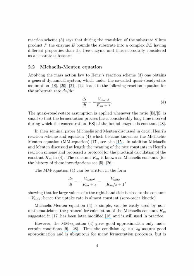
Figure 2: Graphics of the solutions of system (5)

Denote the concentrations s = [S], e = [E], c = [SE], p = [P ].Applying the Mass Action Law to Henri’s reaction scheme (3) we obtainthe general ODEs system:

ds

dt= −k1es+ k−1c,

de

dt= −k1es+ (k−1 + k2)c,

dc

dt= k1es− (k−1 + k2)c,

dp

dt= k2c,

(5)

to be further briefly denoted as HMM-system in tribute to the pioneeringwork of Henri [11]–[14] and Michaelis and Menten [17].

Remark. Note that the Mass Action Law applied to any reactionscheme induces an ODE system in an unique way. For example, in the caseof system (5) the first equation for s says that the rate of change of theconcentration [S] is made up of a loss rate proportional to se = [S][E] anda gain rate proportional to c = [SE].

5

If the rate constants k′s are known, then the HMM-system (5) can betreated as an initial ODE problem with initial conditions s(0) = s0 >0, e(0) = e0 > 0, c(0) = 0, p(0) = 0. However, in practice these constantsare not known and have to be found. The contemporary approach to thistask is to consider the rate constants as parameters in the HMM-system (5)and to compute them by fitting the solutions of the system to available timecourse experimental data, a problem to be considered in the next section.

The graphics of the solutions of the HMM-system (5) for a particularset of initial values and rate constants are presented in Fig. 2.

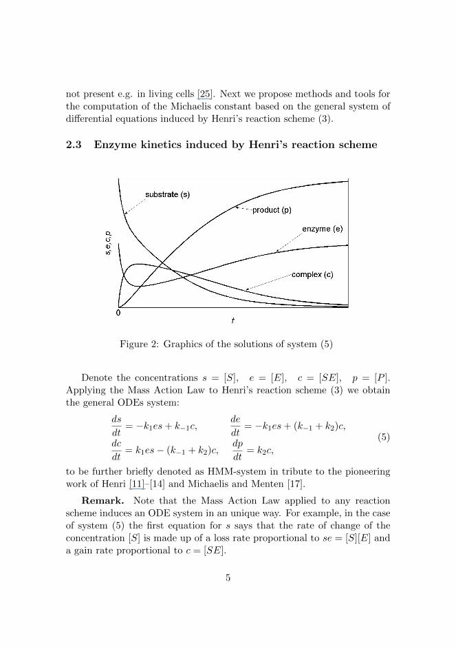
Figure 3: Graphics of the substrate dynamics according to MM-model (4)and HMM-system (5). The rate constants of (5) are k1 = 2.62, k−1 =0.1, k2 = 1.25, initial conditions: s0 = 1, e0 = 1.5; the parameters of (4)can be evaluated to Km = (k−1 + k2)/k1 = 0.51526, Vmax = k2e0 = 1.875

In Fig.3 the substrate uptake s is presented in two different ways. Thetwo graphics present the approximate solution for s to MM-model (4):ds/dt = −Vmaxs/(Km + s) as well as the “true” solution of the HMM-system (5).

6

In order to correctly compare the two solutions one has to establishcertain consistency relations between the parameters in the MM-equationand the HMM-system. The presented solutions in Fig. 3 make use of thefamiliar relations:

Vmax = k2e0Km = (k−1 + k2)/k1,

(6)

induced by the derivation of the MM-equation from the HMM-system usingthe quasi-steady-state assumption, cf. e.g [18].

The following numerical computations show how different the approxi-mate substrate concentration solution s to the MM-equation may look likedepending on the value of the ratio of the initial values of the substrate(s0) and the enzyme (e0).

2.4 Numerical computations of enzyme kinetic models withvarious values for the ratio e0/s0

In this subsection we present the computational results of three numericalexamples for the comparison of the substrate dynamics of the two models(4), (5) for different values of the ratio e0/s0. The values of the initialconditions and the values of the rate constants ki, i = −1, 1, 2 in (5) arechosen to be the same for all three examples. The initial values and therate parameters in (4) are consistent with those in (5); the relations (6):Vmax = k2e0,Km = (k−1 + k2)/k1 have been used.

For completeness we also include the graphics of the solution of simpledecay equation (2). The rate constant k in the decay equation is chosento be equal to k1 and the enzyme concentration e in the right-hand side isfixed as e = e0.

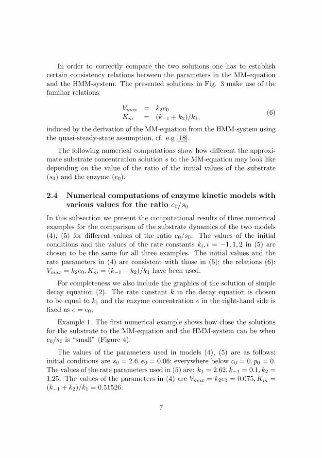
Example 1. The first numerical example shows how close the solutionsfor the substrate to the MM-equation and the HMM-system can be whene0/s0 is “small” (Figure 4).

The values of the parameters used in models (4), (5) are as follows:initial conditions are s0 = 2.6, e0 = 0.06; everywhere below c0 = 0, p0 = 0.The values of the rate parameters used in (5) are: k1 = 2.62, k−1 = 0.1, k2 =1.25. The values of the parameters in (4) are Vmax = k2e0 = 0.075,Km =(k−1 + k2)/k1 = 0.51526.

7

10 20 30 40 50 60 70Time

0.2

0.4

0.6

0.8

1.0

Substrate concentration

First Order Reaction Kinetics ModelEnzyme Kinetics Model - Henri-Michaelis-Menten

Michaelis-Menten Model

Figure 4: The substrate solutions of (4), (5) for e0 << s0

From this numerical example we conclude that when the conditione0 << s0 holds then the MM-model (4) can be a good approximation of the“true” HMM-model (5). The form of the solutions for the substrate con-centrations suggest the hypothesis that whenever the condition e0 << s0holds then the uniform distance between the two solutions is of the orderof the ratio ε = e0/s0. As we know the MM-equation has been derivedfrom the HMM-system under the quasi-steady-state assumption involvingthe condition ε close to zero.

Note that in this example the Michaelis constant Km used for the com-putation of the approximate MM-solution is derived from the coefficientski in the exact HMM-model. This means that both models describe theprocess dynamics using equivalent rate constants and, since we consider theHMM-model to be true, this implies the approximate model is also valid

8

under the assumption e0 << s0. Our next two numerical examples aim todemonstrate what happens whenever this assumption does not hold.

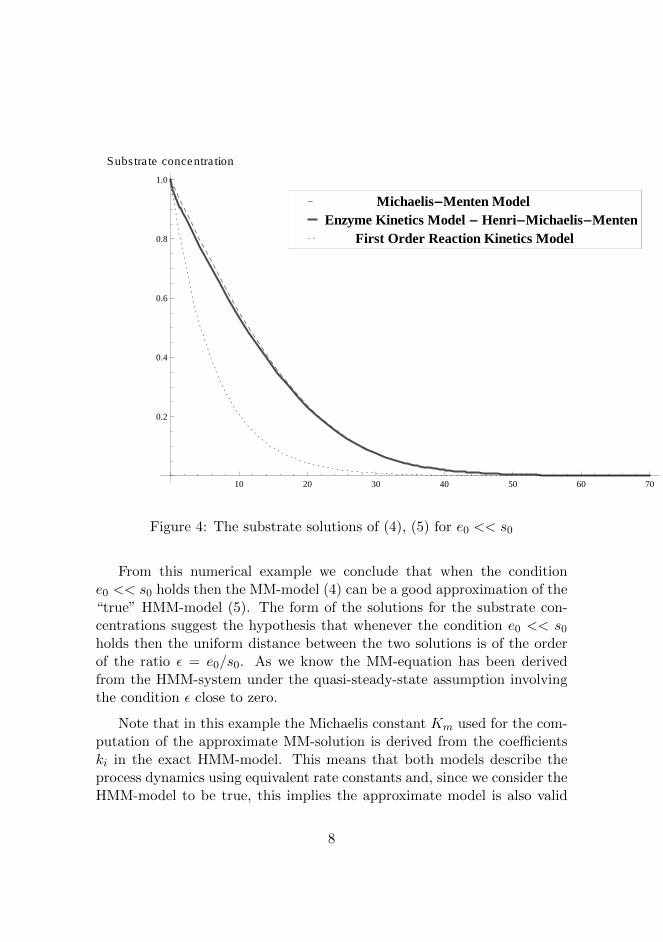
Example 2. Our second numerical example shows how the substratesolutions start to deviate when s0 and e0 are close to each other (Figure 5).

1 2 3 4Time

0.2

0.4

0.6

0.8

1.0

Substrate concentration

First Order Reaction Kinetics ModelEnzyme Kinetics Model - Henri-Michaelis-Menten

Michaelis-Menten Model

Figure 5: The substrate solutions of (4), (5) for e0 ∼ s0.

The values of the parameters used for this example are as follows: s0 =1, e0 = 0.6, k1 = 2.62, k−1 = 0.1, k2 = 1.25. As before, using using (6) weobtain: Vmax = k2e0 = 0.75,Km(k−1 + k2)/k1 = 0.51526.

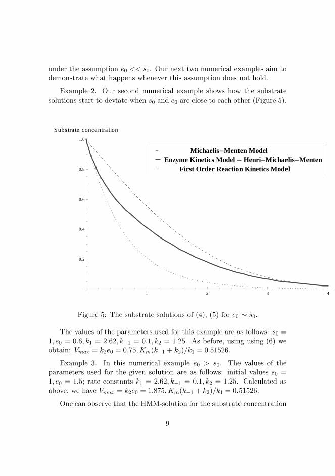
Example 3. In this numerical example e0 > s0. The values of theparameters used for the given solution are as follows: initial values s0 =1, e0 = 1.5; rate constants k1 = 2.62, k−1 = 0.1, k2 = 1.25. Calculated asabove, we have Vmax = k2e0 = 1.875,Km(k−1 + k2)/k1 = 0.51526.

One can observe that the HMM-solution for the substrate concentration

9

is even closer to the exponential decay solution (Figure 6).

0.5 1.0 1.5 2.0Time

0.2

0.4

0.6

0.8

1.0

Substrate concentration

First Order Reaction Kinetics ModelEnzyme Kinetics Model - Henri-Michaelis-Menten

Michaelis-Menten Model

Figure 6: The substrate solutions of (4), (5) for e0 > s0

Examples 2 and 3 clearly show that the MM-model’s solutions are farfrom those of the exact HMM-system despite taking care of the consistencyof the parameters used in (4) and (5). Such a discrepancy between thetwo solutions can be expected as the condition ε close to zero used for thederivation of the approximate MM-model has been violated.

In order to study the dynamics of the fermentation processes, we nextfocus on the HMM-system. Our goal is to obtain a good fit of the HMM-system to available time course experimental data keeping in mind themeasurement errors contained in the data. The model parameters obtainedfrom the fit of the experimental data are then compared to rate constantsfrom the literature corresponding to the same physical processes. This

10

allows us to also verify the correctness of the dynamics suggested by themodel.

Out[4]=

T 16.5

e0 0.46

s0 2.17

k0 0.1

k1 2.62

k2 1.25

XMIN 0

YMIN 0

XMAX 14.

YMAX 2.222380 2 4 6 8 10 12 14

0.0

0.5

1.0

1.5

2.0

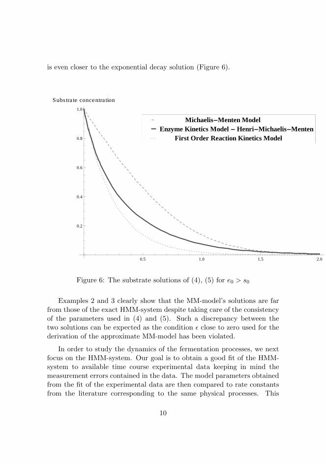
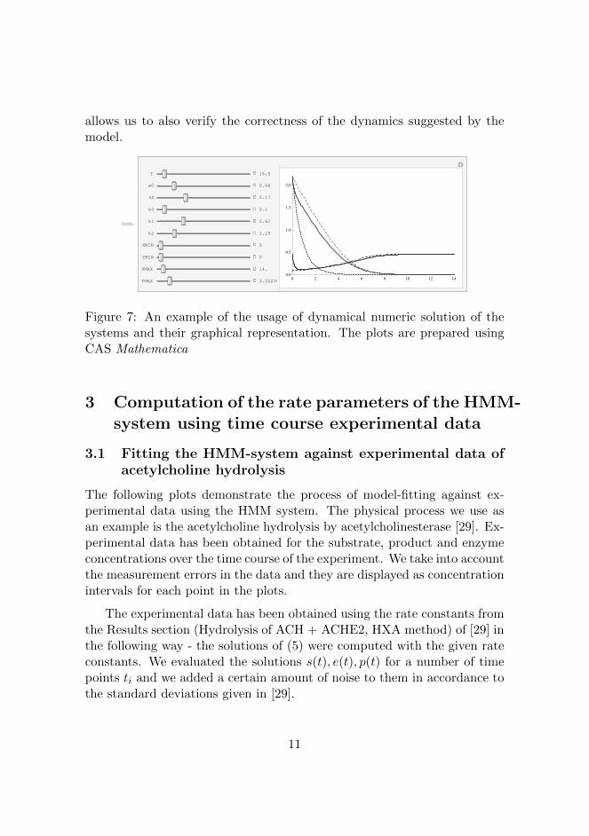
Figure 7: An example of the usage of dynamical numeric solution of thesystems and their graphical representation. The plots are prepared usingCAS Mathematica

3 Computation of the rate parameters of the HMM-system using time course experimental data

3.1 Fitting the HMM-system against experimental data ofacetylcholine hydrolysis

The following plots demonstrate the process of model-fitting against ex-perimental data using the HMM system. The physical process we use asan example is the acetylcholine hydrolysis by acetylcholinesterase [29]. Ex-perimental data has been obtained for the substrate, product and enzymeconcentrations over the time course of the experiment. We take into accountthe measurement errors in the data and they are displayed as concentrationintervals for each point in the plots.

The experimental data has been obtained using the rate constants fromthe Results section (Hydrolysis of ACH + ACHE2, HXA method) of [29] inthe following way - the solutions of (5) were computed with the given rateconstants. We evaluated the solutions s(t), e(t), p(t) for a number of timepoints ti and we added a certain amount of noise to them in accordance tothe standard deviations given in [29].

11

Our computational problem can be formulated as follows. Given timecourse experimental data (together with measurement errors) for the sub-strate, enzyme and product concentrations find values for the parametersk−1, k1, k2 and initial values E0, s0 such that the solution of the HMM sys-tem (5) fit well against the experimental data and possibly fit into themeasurement intervals. Our procedure for solving this problem passes intwo stages: first we find an initial rough “guess” for the parameter values,then we consecutively improve the parameter set, resp. the solutions, usingsome optimization possibilities of the numerical computing environmentMATLAB. More precisely, we’ve used MATLAB’s lsqnonlin procedure (op-timization algorithm defaults to Trust-Region-Reflective Algorithm), wherethe minimized function 1) computes the enzyme kinetics model solutions(using ode23 or ode23s solvers) for a given set of rate constants and initialconditions (optimization procedure parameters), 2) evaluates the solutionsfor the time points ti corresponding to the observations and 3) subtractsthe experimental data from them.

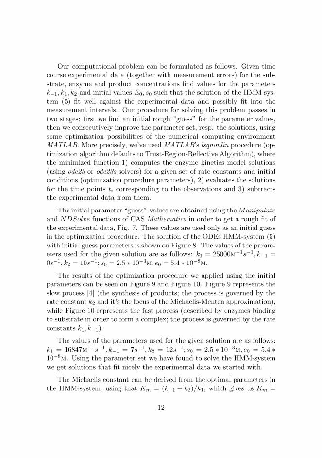
The initial parameter “guess”-values are obtained using the Manipulateand NDSolve functions of CAS Mathematica in order to get a rough fit ofthe experimental data, Fig. 7. These values are used only as an initial guessin the optimization procedure. The solution of the ODEs HMM-system (5)with initial guess parameters is shown on Figure 8. The values of the param-eters used for the given solution are as follows: k1 = 25000m−1s−1, k−1 =0s−1, k2 = 10s−1; s0 = 2.5 ∗ 10−3m, e0 = 5.4 ∗ 10−8m.

The results of the optimization procedure we applied using the initialparameters can be seen on Figure 9 and Figure 10. Figure 9 represents theslow process [4] (the synthesis of products; the process is governed by therate constant k2 and it’s the focus of the Michaelis-Menten approximation),while Figure 10 represents the fast process (described by enzymes bindingto substrate in order to form a complex; the process is governed by the rateconstants k1, k−1).

The values of the parameters used for the given solution are as follows:k1 = 16847m−1s−1, k−1 = 7s−1, k2 = 12s−1; s0 = 2.5 ∗ 10−3m, e0 = 5.4 ∗10−8m. Using the parameter set we have found to solve the HMM-systemwe get solutions that fit nicely the experimental data we started with.

The Michaelis constant can be derived from the optimal parameters inthe HMM-system, using that Km = (k−1 + k2)/k1, which gives us Km =

12

0 2000 4000 6000 8000 10000 12000 140000

1

2

3

x 10−3

Reaction time [seconds]

Concentr

ation (

substr

ate

, pro

duct [m

M])

Enzyme Kinetics Model

0 2000 4000 6000 8000 10000 12000 140000

0.2

0.4

0.6

x 10−7

Concentr

ation −

enzym

e, com

ple

x [m

M]

substrate − s

product − p

experimental data − s

experimental data − p

enzyme e

complex c

experimental data − e

errors

Figure 8: The numerical solution of the HMM-system with an initial pa-rameter “guess” set of the unknown parameters

13

0 2000 4000 6000 8000 10000 12000 140000

0.5

1

1.5

2

2.5

x 10−3

Reaction time [seconds]

Concentr

ation (

substr

ate

, pro

duct [m

M])

Enzyme Kinetics Model

0 2000 4000 6000 8000 10000 12000 14000

0.1

0.2

0.3

0.4

0.5

0.6

x 10−7

Concentr

ation −

enzym

e, com

ple

x [m

M]

substrate − s

product − p

experimental data − s

experimental data − p

enzyme e

complex c

experimental data − e

errors

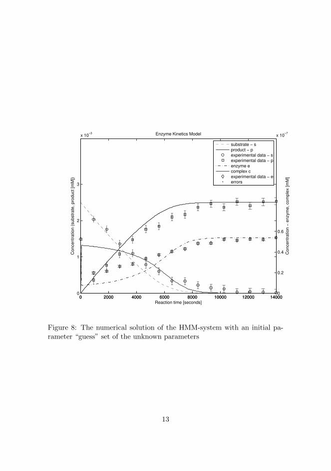
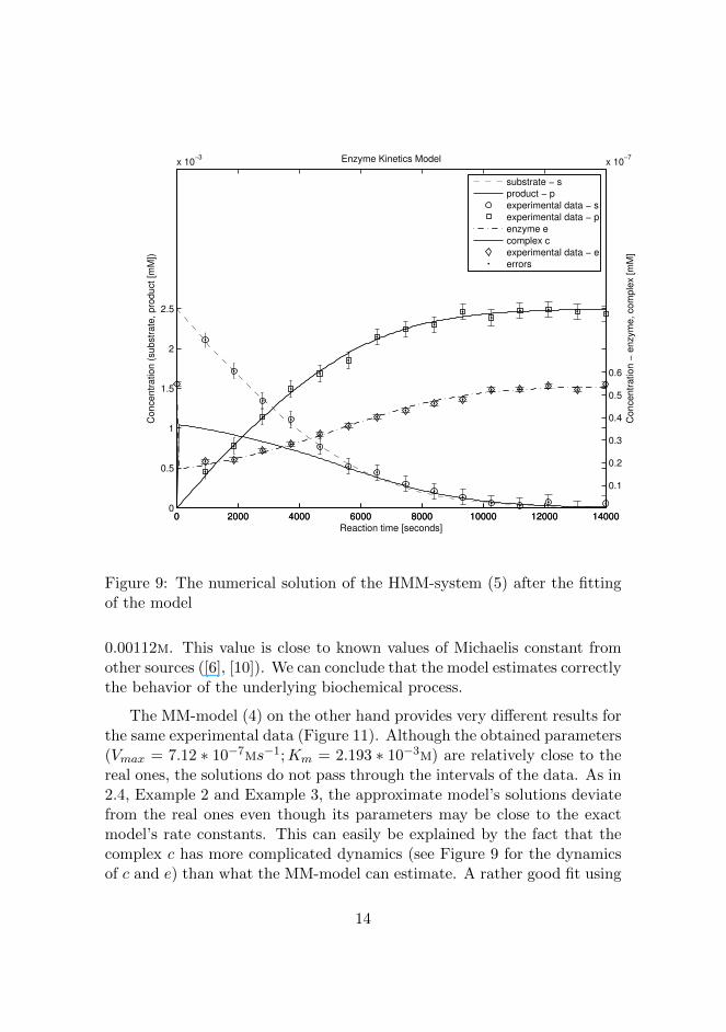
Figure 9: The numerical solution of the HMM-system (5) after the fittingof the model

0.00112m. This value is close to known values of Michaelis constant fromother sources ([6], [10]). We can conclude that the model estimates correctlythe behavior of the underlying biochemical process.

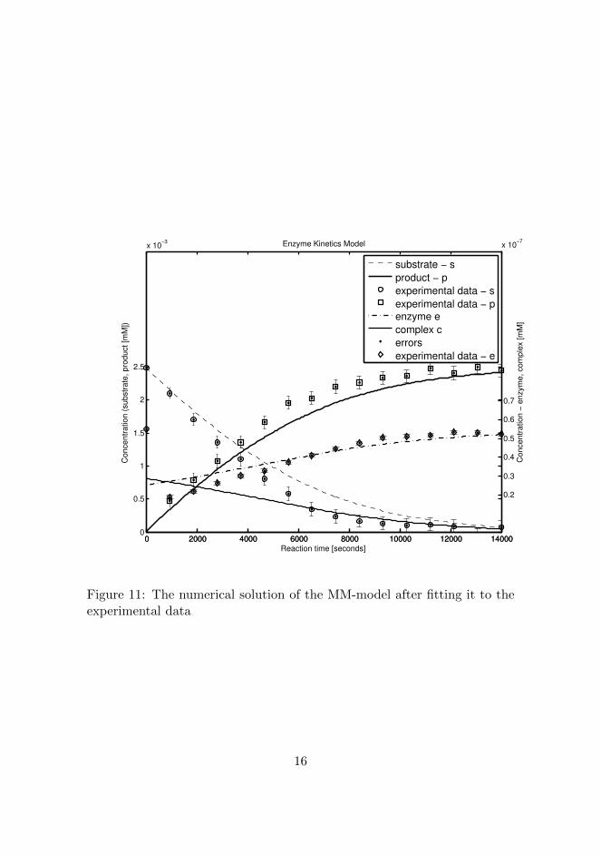
The MM-model (4) on the other hand provides very different results forthe same experimental data (Figure 11). Although the obtained parameters(Vmax = 7.12 ∗ 10−7ms−1;Km = 2.193 ∗ 10−3m) are relatively close to thereal ones, the solutions do not pass through the intervals of the data. As in2.4, Example 2 and Example 3, the approximate model’s solutions deviatefrom the real ones even though its parameters may be close to the exactmodel’s rate constants. This can easily be explained by the fact that thecomplex c has more complicated dynamics (see Figure 9 for the dynamicsof c and e) than what the MM-model can estimate. A rather good fit using

14

0 10 20 30 40 50 60 70 800

2.4425x 10

−3

Reaction time [seconds]

Concentr

ation (

substr

ate

, pro

duct [m

M])

Enzyme Kinetics Model

0 10 20 30 40 50 60 70 80

0.1

0.2

0.3

0.4

0.5

0.6

x 10−7

Concentr

ation −

enzym

e, com

ple

x [m

M]

substrate − s

product − p

enzyme e

complex c

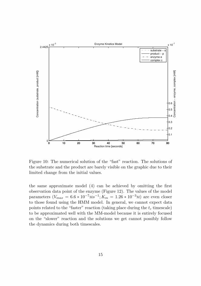
Figure 10: The numerical solution of the “fast” reaction. The solutions ofthe substrate and the product are barely visible on the graphic due to theirlimited change from the initial values.

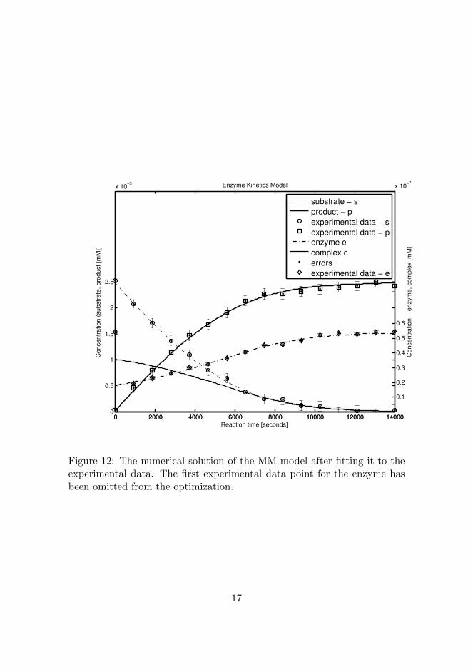
the same approximate model (4) can be achieved by omitting the firstobservation data point of the enzyme (Figure 12). The values of the modelparameters (Vmax = 6.6 ∗ 10−7ms−1;Km = 1.26 ∗ 10−3m) are even closerto those found using the HMM model. In general, we cannot expect datapoints related to the “faster” reaction (taking place during the tc timescale)to be approximated well with the MM-model because it is entirely focusedon the “slower” reaction and the solutions we get cannot possibly followthe dynamics during both timescales.

15

0 2000 4000 6000 8000 10000 12000 140000

0.5

1

1.5

2

2.5

x 10−3

Reaction time [seconds]

Concentr

ation (

substr

ate

, pro

duct [m

M])

Enzyme Kinetics Model

0 2000 4000 6000 8000 10000 12000 14000

0.2

0.3

0.4

0.5

0.6

0.7

x 10−7

Concentr

ation −

enzym

e, com

ple

x [m

M]

substrate − s

product − p

experimental data − s

experimental data − p

enzyme e

complex c

errors

experimental data − e

Figure 11: The numerical solution of the MM-model after fitting it to theexperimental data

16

0 2000 4000 6000 8000 10000 12000 140000

0.5

1

1.5

2

2.5

x 10−3

Reaction time [seconds]

Concentr

ation (

substr

ate

, pro

duct [m

M])

Enzyme Kinetics Model

0 2000 4000 6000 8000 10000 12000 14000

0.1

0.2

0.3

0.4

0.5

0.6

x 10−7

Concentr

ation −

enzym

e, com

ple

x [m

M]

substrate − s

product − p

experimental data − s

experimental data − p

enzyme e

complex c

errors

experimental data − e

Figure 12: The numerical solution of the MM-model after fitting it to theexperimental data. The first experimental data point for the enzyme hasbeen omitted from the optimization.

17

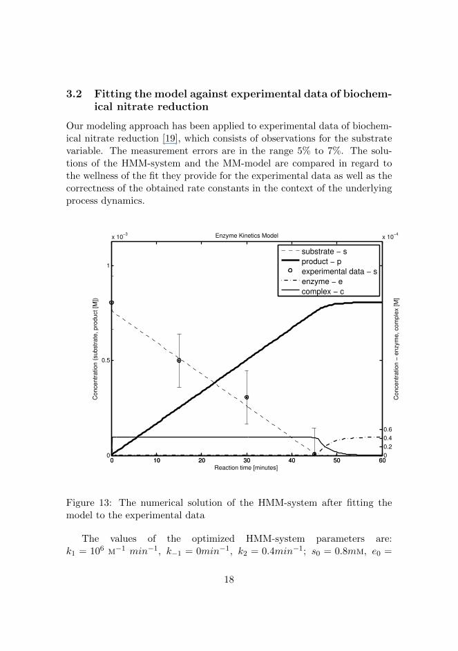
3.2 Fitting the model against experimental data of biochem-ical nitrate reduction

Our modeling approach has been applied to experimental data of biochem-ical nitrate reduction [19], which consists of observations for the substratevariable. The measurement errors are in the range 5% to 7%. The solu-tions of the HMM-system and the MM-model are compared in regard tothe wellness of the fit they provide for the experimental data as well as thecorrectness of the obtained rate constants in the context of the underlyingprocess dynamics.

0 10 20 30 40 50 600

0.5

1

x 10−3

Reaction time [minutes]

Concentr

ation (

substr

ate

, pro

duct [M

])

Enzyme Kinetics Model

0 10 20 30 40 50 600

0.2

0.4

0.6

x 10−4

Concentr

ation −

enzym

e, com

ple

x [M

]

substrate − s

product − p

experimental data − s

enzyme − e

complex − c

Figure 13: The numerical solution of the HMM-system after fitting themodel to the experimental data

The values of the optimized HMM-system parameters are:k1 = 106 m−1 min−1, k−1 = 0min−1, k2 = 0.4min−1; s0 = 0.8mm, e0 =

18

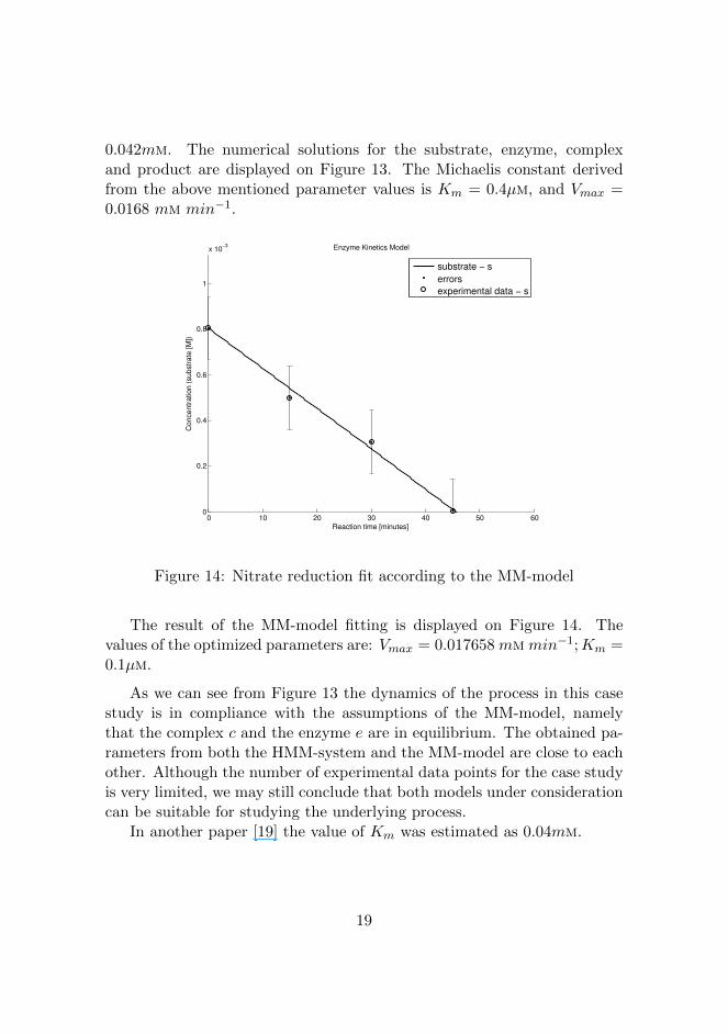
0.042mm. The numerical solutions for the substrate, enzyme, complexand product are displayed on Figure 13. The Michaelis constant derivedfrom the above mentioned parameter values is Km = 0.4µm, and Vmax =0.0168 mm min−1.

0 10 20 30 40 50 600

0.2

0.4

0.6

0.8

1

x 10−3

Reaction time [minutes]

Concentr

ation (

su

bstr

ate

[M

])

Enzyme Kinetics Model

substrate − s

errors

experimental data − s

Figure 14: Nitrate reduction fit according to the MM-model

The result of the MM-model fitting is displayed on Figure 14. Thevalues of the optimized parameters are: Vmax = 0.017658 mmmin−1;Km =0.1µm.

As we can see from Figure 13 the dynamics of the process in this casestudy is in compliance with the assumptions of the MM-model, namelythat the complex c and the enzyme e are in equilibrium. The obtained pa-rameters from both the HMM-system and the MM-model are close to eachother. Although the number of experimental data points for the case studyis very limited, we may still conclude that both models under considerationcan be suitable for studying the underlying process.

In another paper [19] the value of Km was estimated as 0.04mm.

19

4 Concluding remarks

The present paper is devoted to computational experiments for the clas-sic Henri-Michaelis-Menten enzyme kinetic scheme and the approximateMichaelis-Menten model, derived under the quasi-steady-state assumption.A comparison of the results from the two models with experimental datais also shown. The given examples demonstrate the advantages of the ex-act model in comparison to the approximate models. The topic has beenthoroughly analyzed by other authors [31] in terms of the magnitude of theerror of the approximate models and the conditions under which they areadequate. In this paper we present an approach of numerical analysis ap-plying the model proposed by V. Henri, while using contemporary softwaretools.

There are many benefits of using the Henri’s reaction scheme whenstudying biological processes. Even complex systems (e.g. metabolic net-works) with many reactants or consisting of several interconnected Michaelis-Menten reactions can be modeled accurately in contrast to simpler modelswhere many approximations may contradict with the behavior of the wholesystem. Working with models that follow directly from physical/chemicallaws allows for deeper, more serious analysis of the process due to the levelof detail they provide over the reactions that take part in it. For example,all rate constants ki have been obtained for the considered models partof our case studies which could be essential to subsequent analysis. Fur-thermore, the parameters of the approximate model can also be obtainedfrom these rate constants, allowing us to validate our results against knownvalues of the classic Michaelis constant.

Such approximate models may have been used with more care in thepast since they are computationally intensive when it comes to numericalexperiments, but this should hardly be considered an issue nowadays. Thereare also very rich software products which provide powerful tools for thenumerical experiments and analysis of complex physical processes.

A topic worth further analysis as a potential future direction would bewhether we could fit a time series using Calder’s sigma-isocline [30] insteadof the QSSA.

20

5 Acknowledgements

This work was accomplished within the project HYSULFCEL supportedby the programme BS-ERA.NET (FP7 of the European Union), grantDNS7FP 01/32 of the Ministry of Education and Science, Republic of Bul-garia.

References

[1] Berberan-Santos, Mario, N., A General Treatment of Henri-Michaelis-Menten Enzyme Kinetics: Exact Series Solution and Approximate An-alytical Solutions, MATCH Commun. Math. Comput. Chem. 63, 283–318, 2010.

[2] Beschkov, V., S. Velizarov, S. N. Agathos, V. Lukova, Bacterial deni-trification of wastewater stimulated by constant electric field, The Bio-chemical Engineering Journal 17 (2), 141–145 (2004).

[3] Cermak, Nate, Fundamentals of Enzyme Kinetics: Michaelis-Mentenand Deviations, 2009http://cermak.scripts.mit.edu/papers/

383final cermak enzymekinetics 20090312.pdf

[4] Chen, William W., Mario Niepel, Peter K. Sorger, Classic and contem-porary approaches to modeling biochemical reactions, Genes Dev 24:1861–1875 (2010).

[5] Deichmann, U., S. Schuster, J.-P. Mazat, A. Cornish-Bowden, Commemorating the 1913 Michaelis-Menten paperDie Kinetik der Invertinwirkung: three perspectives, FEBSJournal 281 (2014), 435–463. (see Part 3: before Michaelisand Menten: Victor Henris equation by Jean-Pierre Mazat)http://onlinelibrary.wiley.com/doi/10.1111/febs.12598/pdf

[6] Forsberg, Ake, Kinetics for the inhibition of acetylcholinesterase fromthe electric eel by some organophosphates and carbamates, Eur. J .Biochem. 140, 153–156 (1984).

21

[7] Goudar, C.T., J.R. Sonnad, R.G. Duggleby, Parameter estimation usinga direct solution of the integrated Michaelis-Menten equation, Biochim-ica et Biophysica Acta 1429 (1999), 377–383.

[8] Goudar, C.T., S.K. Harris, M.J. McInerney, J.M Suflita (2004). Progresscurve analysis for enzyme and microbial kinetic reactions using explicitsolutions based on the Lambert W-function. Journal of MicrobiologicalMethods 59, 317–326.

[9] Grima, R., N. G. Walter, S. Schnell, Single molecule enzymologya la Michaelis-Menten. FEBS Journal 281, (2014) 518–530. DOI:10.1111/febs.12663

[10] Hai, Aviad, et al., Acetylcholinesterase-ISFET based system for thedetection of acetylcholine and acetylcholinesterase inhibitors, Biosensorsand Bioelectronics 22 (2006), 605–612.

[11] Henri, V., Recherches sur la loi de laction de la sucrase. C. R. Hebd.Acad. Sci., 133, 891–899 (1901).

[12] Henri, V., Ueber das Gesetz der Wirkung des Invertins. Z. Phys.Chem., 39 (1901), 194–216.

[13] Henri ,V., (1902) Theorie generale de laction de quelques diastases. CR Hebd Seances Acad Sci 135, 916–919.

[14] Henri, V., (1903) Lois generales de laction des diastases. Hermann,Paris.

[15] Johnson, Kenneth A., Roger S. Goody, The Original Michaelis Con-stant: Translation of the 1913 Michaelis–Menten Paper, Biochemistry,50 (39): 8264–8269, 2011.doi:10.1021/bi201284u.

[16] Lineweaver, H., D. Burk, The Determination of Enzyme DissociationConstants, Journal of the American Chemical Society 56 (3): 658–666,1934. // doi:10.1021/ja01318a036.

[17] Michaelis, L., M. L. Menten. Die Kinetik der Invertinwirkung.Biochem. Z. 49, (1913), 333–369.

22

[18] Murray J. D., Mathematical Biology: I. An Introduction, Third Edi-tion, Springer, 2002.

[19] Parvanova-Mancheva Ts., V. Beschkov, Ts. Sapundzhiev, Modeling ofbiochemical nitrate reduction in constant electric field, Chemical andBiochemical Engineering Quarterly, 23 (1), 67-75 (2009)

[20] Pedersen, Morten Gram, Alberto M. Bersani, Enrico Bersani, Giu-liana Cortese, The total quasi-steady-state approximation for complexenzyme reactions, Mathematics and Computers in Simulation 79 (2008)1010–1019.

[21] Roussel, M.R., S.J. Fraser, Accurate steady-state approximations: Im-plications for kinetics experiments and mechanism, J. Phys. Chem. 95(1991) 8762–8770.

[22] Roussel, M.R., A rigorous approach to steady-state kinetics appliedto simple enzyme mechanisms, PhD thesis, Department of Chemistry,University of Toronto, 1994.

[23] Schnell, S., C. Mendoza, A closed form solution for time-dependentenzyme kinetics. Journal of theoretical Biology, 187 (1997): 207–212.http://dx.doi.org/10.1006/jtbi.1997.0425

[24] S. Schnell, C. Mendoza, Time-dependent closed form solution forfully competitive enzyme kinetics, Bulletin of Mathematical Biology62 (2000), 321–336.

[25] Schnell, S., P. K. Maini. 2000. Enzyme kinetics at high enzyme con-centration. Bull. Math. Biol. 62, 483–499.

[26] Schnell, S., P. K. Maini (2003). A century of enzyme kinetics: Relia-bility of the Km and vmax estimates. Comments on Theoretical Biology8, 169–187.

[27] Schnell, S., Chappell, M. J., Evans, N. D., M. R. Roussel, The mech-anism distinguishability problem in biochemical kinetics: The single-enzyme single-substrate reaction as a case study. C. R. Biologies 329,51–61 (2006).

23

[28] Schnell, S., Validity of the Michaelis-Menten equation - Steady-state,or reactant stationary assumption: that is the question. FEBS Journal281, (2014) 464–472. DOI: 10.1111/febs.12564

[29] Zdrazilova, P. et al., Kinetics of Total Enzymatic Hydrolysis of Acetyl-choline and Acetylthiocholine, Zeitschrift fur Naturforschung 61 (3–4),289–294, 2006.

[30] M. S. Calder, D. Siegel, Properties of the Michaelis-Menten mechanismin phase space, J. Math. Anal. Appl. 339 (2008) 1044-1064.

[31] R. F. Brown, M. T. Holtzapple, Parametric Analysis of the Errors As-sociated with the Michaelis-Menten Equation, Biotechnology and Bio-engineering. 36 (11) (1990) 1141-1150

24