on the inverse problem for finite dissipative jacobi matrices ...

Commun. Fac. Sci. Univ. Ank. Ser. A1 Math. Stat.Volume 68, Number 2, Pages 1273—1288 (2019)DOI: 10.31801/cfsuasmas.419098ISSN 1303—5991 E-ISSN 2618-6470

Available online: January 28, 2019

http://communications.science.ankara.edu.tr/index.php?series=A1

ON THE INVERSE PROBLEM FOR FINITE DISSIPATIVEJACOBI MATRICES WITH A RANK-ONE IMAGINARY PART

EBRU ERGUN

Abstract. This paper deals with the inverse spectral problem consisting inthe reconstruction of a finite dissipative Jacobi matrix with a rank-one imagi-nary part from its eigenvalues. Necessary and suffi cient conditions are formu-lated for a prescribed collection of complex numbers to be the spectrum of afinite dissipative Jacobi matrix with a rank-one imaginary part. Uniquenessof the matrix having prescribed eigenvalues is shown and an algorithm forreconstruction of the matrix from prescribed eigenvalues is given.

1. Introduction

An N ×N (real) Jacobi matrix is a tri-diagonal symmetric matrix of the form

J =

b0 a0 0 · · · 0 0 0a0 b1 a1 · · · 0 0 00 a1 b2 · · · 0 0 0...

......

. . ....

......

0 0 0 . . . bN−3 aN−3 00 0 0 · · · aN−3 bN−2 aN−20 0 0 · · · 0 aN−2 bN−1

, (1)

where for each n, an and bn are arbitrary real numbers such that an is positive:

an > 0, bn ∈ R. (2)

Quantities connected with the eigenvalues and eigenvectors of the matrix are calledthe spectral characteristics of the matrix. The general inverse spectral problem isto reconstruct the matrix given some of its spectral characteristics (spectral data).Many versions of the inverse spectral problem for finite and infinite Jacobi matriceshave been investigated in the literature and many procedures and algorithms for

Received by the editors: April 27, 2018; Accepted: August 07, 2018.2010 Mathematics Subject Classification. 15A29.Key words and phrases. Jacobi matrix, eigenvalue, normalizing number, dissipative, inverse

spectral problem.

c©2019 Ankara UniversityCommunications Facu lty of Sciences University of Ankara-Series A1 Mathematics and Statistics

1273

1274 EBRU ERGUN

their solution have been proposed (for some of them see [12, 13, 11, 7, 3, 2, 6, 15,8, 9, 10, 14, 16]).Note that, in general, one spectrum consisting of the eigenvalues of the Jacobi

matrix does not determine this matrix. It turns out that the eigenvalues togetherwith the normalizing numbers (a spectral measure) or the so-called two-spectra areenough to determine the Jacobi matrix uniquely.Now let us along with the matrix J given by (1), (2) consider also the matrix

J =

b0 a0 0 · · · 0 0 0a0 b1 a1 · · · 0 0 00 a1 b2 · · · 0 0 0...

......

. . ....

......

0 0 0 . . . bN−3 aN−3 00 0 0 · · · aN−3 bN−2 aN−20 0 0 · · · 0 aN−2 bN−1

(3)

in which all an and bn are the same as in J, except b0 which is replaced by b0 andwe will assume that

b0 = b0 + iω, ω > 0. (4)

Therefore J is a dissipative matrix with a rank-one imaginary part. It turns out thatthe matrix J has N, counting algebraic multiplicity, nonreal eigenvalues λ1, . . . , λNwith positive imaginary parts. These eigenvalues are determined by their N free,in general, real parts and N free positive imaginary parts. The matrix J alsocontains N free real parameters b0, b1, . . . , bN−1 and N free positive parametersa0, a1, . . . , aN−2 and ω. Therefore one may expect that the inverse problem fromthe eigenvalues λ1, . . . , λN to the matrix J is uniquely solvable. Such an inverseproblem was recently investigated and solved in the paper [1] by using the Livsiccharacteristic function of the matrix J and expansion into continuous fractions ofthe Weyl-Titchmarsh function of J , expressed in terms of the Livsic characteristicfunction.In the present paper, we revisit the reconstruction problem of a dissipative Jacobi

matrix with a rank-one imaginary part from its eigenvalues. Our approach to thisproblem in this paper differs from that in the paper [1] and is based on a known facton polynomials with roots in the open upper half-plane (Theorem 2 below in Section2) and on the reduction of the inverse problem for the dissipative Jacobi matrixJ of the form (3), (4) to the inverse problem from two-spectra for the associatedreal Jacobi matrix J defined by (1), (2). Besides, the latter problem we solve bythe discrete Gelfand-Levitan method instead of the continuous fraction expansion.We hope that the approach suggested in the present paper may contribute someadditional insights to the theory of inverse problems for dissipative Jacobi matricesand may be useful in related problems.

ON THE INVERSE PROBLEM FOR FINITE DISSIPATIVE JACOBI MATRICES 1275

The paper consists, besides this introductory section, of four sections. In Section2, we formulate a solution procedure of the inverse problem for real Jacobi matricesfrom the eigenvalues and normalizing numbers and also from the two-spectra, andpresent a known theorem on the polynomials with roots in the open upper half-plane. In Section 3, we deal with the inverse problem for dissipative Jacobi matriceswith a rank-one imaginary part from its eigenvalues and establish necessary andsuffi cient conditions for solvability of the inverse problem. In Section 4, we describethe reconstruction procedure and give an example. Finally, in Section 5, we makesome concluding remarks on the reconstruction procedure.

2. Auxiliary facts

In this section, we present briefly known solutions of the inverse problems withrespect to eigenvalues and normalizing numbers and with respect to two-spectra,for real finite Jacobi matrices. Also, we present a known theorem on complexpolynomials with zeros in the open upper half-plane. This knowledge is given herefor easy reference and they will be used in the subsequent sections.1. It is well known that any real Jacobi matrix of the form (1), (2) has precisely

N real and distinct eigenvalues λ1, . . . , λN , so

det(λI − J) = (λ− λ1) · · · (λ− λN ). (5)

The normalizing numbers of the matrix J can be introduced as follows. Let R(λ) =(J − λI)−1 be the resolvent of the matrix J (by I we denote the identity matrix ofneeded dimension) and e0 be theN -dimensional column vector with the components1, 0, . . . , 0. The rational function

w(λ) = −〈R(λ)e0, e0〉 =⟨(λI − J)−1e0, e0

⟩, (6)

introduced earlier in [13], is called the resolvent function of the matrix J, where〈·, ·〉 denotes the standard inner product in CN . This function is known also as theWeyl or Weyl-Titchmarsh function of J. The resolvent function w(λ) admits, by(6) and (5), the decomposition into partial fractions,

w(λ) =

N∑k=1

βkλ− λk

, (7)

where βk’s are some positive real numbers uniquely determined by the matrix Jand such that

N∑k=1

βk = 1. (8)

The number βk is called the normalizing number of the matrix J, associated withthe eigenvalue λk (it is related to the norm of the eigenvector of J, correspondingto the eigenvalue λk).The collection of the eigenvalues and normalizing numbers

{λk, βk (k = 1, . . . , N)} (9)

1276 EBRU ERGUN

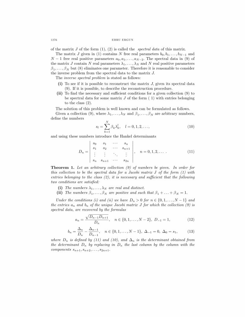
of the matrix J of the form (1), (2) is called the spectral data of this matrix.The matrix J given in (1) contains N free real parameters b0, b1, . . . , bN−1 and

N − 1 free real positive parameters a0, a1, . . . , aN−2. The spectral data in (9) ofthe matrix J contain N real parameters λ1, . . . , λN and N real positive parametersβ1, . . . , βN but (8) eliminates one parameter. Therefore it is reasonable to considerthe inverse problem from the spectral data to the matrix J.The inverse spectral problem is stated as follows:

(i) To see if it is possible to reconstruct the matrix J, given its spectral data(9). If it is possible, to describe the reconstruction procedure.

(ii) To find the necessary and suffi cient conditions for a given collection (9) tobe spectral data for some matrix J of the form ( 1) with entries belongingto the class (2).

The solution of this problem is well known and can be formulated as follows.Given a collection (9), where λ1, . . . , λN and β1, . . . , βN are arbitrary numbers,

define the numbers

sl =

N∑k=1

βkλlk, l = 0, 1, 2, . . . , (10)

and using these numbers introduce the Hankel determinants

Dn =

∣∣∣∣∣∣∣∣∣s0 s1 · · · sns1 s2 · · · sn+1...

.... . .

...sn sn+1 · · · s2n

∣∣∣∣∣∣∣∣∣ , n = 0, 1, 2, . . . . (11)

Theorem 1. Let an arbitrary collection (9) of numbers be given. In order forthis collection to be the spectral data for a Jacobi matrix J of the form (1) withentries belonging to the class (2), it is necessary and suffi cient that the followingtwo conditions are satisfied:

(i) The numbers λ1, . . . , λN are real and distinct.(ii) The numbers β1, . . . , βN are positive and such that β1 + . . .+ βN = 1.

Under the conditions (i) and (ii) we have Dn > 0 for n ∈ {0, 1, . . . , N − 1} andthe entries an and bn of the unique Jacobi matrix J for which the collection (9) isspectral data, are recovered by the formulas

an =

√Dn−1Dn+1

Dn, n ∈ {0, 1, . . . , N − 2}, D−1 = 1, (12)

bn =∆n

Dn− ∆n−1Dn−1

, n ∈ {0, 1, . . . , N − 1}, ∆−1 = 0, ∆0 = s1, (13)

where Dn is defined by (11) and (10), and ∆n is the determinant obtained fromthe determinant Dn by replacing in Dn the last column by the column with thecomponents sn+1, sn+2, . . . , s2n+1.


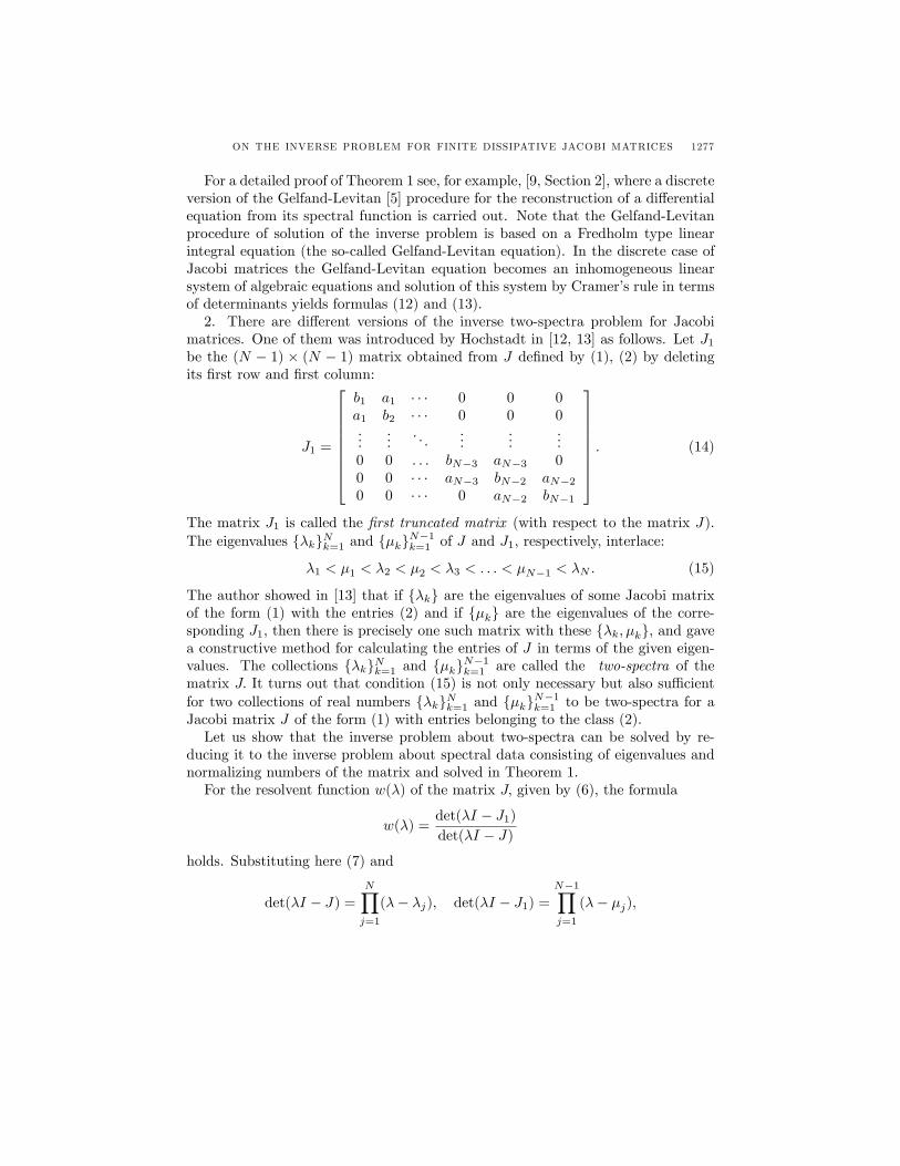
For a detailed proof of Theorem 1 see, for example, [9, Section 2], where a discreteversion of the Gelfand-Levitan [5] procedure for the reconstruction of a differentialequation from its spectral function is carried out. Note that the Gelfand-Levitanprocedure of solution of the inverse problem is based on a Fredholm type linearintegral equation (the so-called Gelfand-Levitan equation). In the discrete case ofJacobi matrices the Gelfand-Levitan equation becomes an inhomogeneous linearsystem of algebraic equations and solution of this system by Cramer’s rule in termsof determinants yields formulas (12) and (13).2. There are different versions of the inverse two-spectra problem for Jacobi

matrices. One of them was introduced by Hochstadt in [12, 13] as follows. Let J1be the (N − 1) × (N − 1) matrix obtained from J defined by (1), (2) by deletingits first row and first column:

J1 =

b1 a1 · · · 0 0 0a1 b2 · · · 0 0 0...

.... . .

......

...0 0 . . . bN−3 aN−3 00 0 · · · aN−3 bN−2 aN−20 0 · · · 0 aN−2 bN−1

. (14)

The matrix J1 is called the first truncated matrix (with respect to the matrix J).The eigenvalues {λk}Nk=1 and {µk}

N−1k=1 of J and J1, respectively, interlace:

λ1 < µ1 < λ2 < µ2 < λ3 < . . . < µN−1 < λN . (15)

The author showed in [13] that if {λk} are the eigenvalues of some Jacobi matrixof the form (1) with the entries (2) and if {µk} are the eigenvalues of the corre-sponding J1, then there is precisely one such matrix with these {λk, µk}, and gavea constructive method for calculating the entries of J in terms of the given eigen-values. The collections {λk}Nk=1 and {µk}

N−1k=1 are called the two-spectra of the

matrix J. It turns out that condition (15) is not only necessary but also suffi cientfor two collections of real numbers {λk}Nk=1 and {µk}

N−1k=1 to be two-spectra for a

Jacobi matrix J of the form (1) with entries belonging to the class (2).Let us show that the inverse problem about two-spectra can be solved by re-

ducing it to the inverse problem about spectral data consisting of eigenvalues andnormalizing numbers of the matrix and solved in Theorem 1.For the resolvent function w(λ) of the matrix J, given by (6), the formula

w(λ) =det(λI − J1)det(λI − J)

holds. Substituting here (7) and

det(λI − J) =

N∏j=1

(λ− λj), det(λI − J1) =

N−1∏j=1

(λ− µj),

1278 EBRU ERGUN

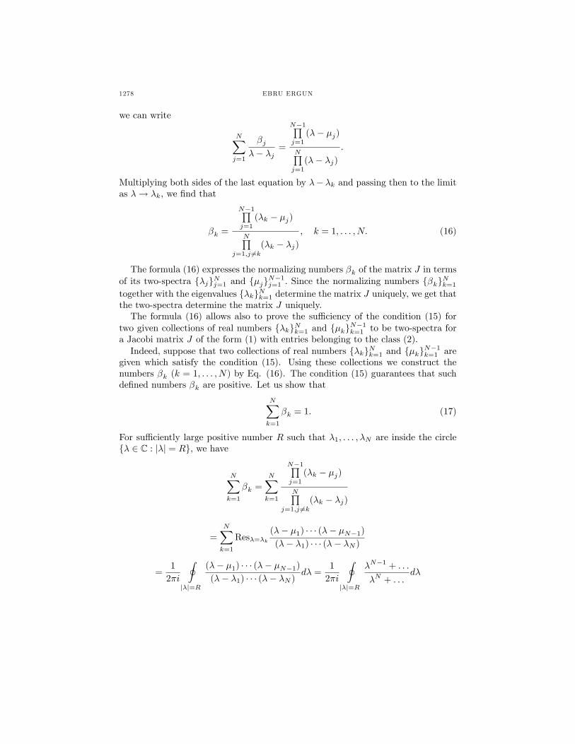
we can write

N∑j=1

βjλ− λj

=

N−1∏j=1

(λ− µj)

N∏j=1

(λ− λj).

Multiplying both sides of the last equation by λ− λk and passing then to the limitas λ→ λk, we find that

βk =

N−1∏j=1

(λk − µj)

N∏j=1,j 6=k

(λk − λj), k = 1, . . . , N. (16)

The formula (16) expresses the normalizing numbers βk of the matrix J in termsof its two-spectra {λj}Nj=1 and {µj}N−1j=1 . Since the normalizing numbers {βk}Nk=1together with the eigenvalues {λk}Nk=1 determine the matrix J uniquely, we get thatthe two-spectra determine the matrix J uniquely.The formula (16) allows also to prove the suffi ciency of the condition (15) for

two given collections of real numbers {λk}Nk=1 and {µk}N−1k=1 to be two-spectra for

a Jacobi matrix J of the form (1) with entries belonging to the class (2).Indeed, suppose that two collections of real numbers {λk}Nk=1 and {µk}

N−1k=1 are

given which satisfy the condition (15). Using these collections we construct thenumbers βk (k = 1, . . . , N) by Eq. (16). The condition (15) guarantees that suchdefined numbers βk are positive. Let us show that

N∑k=1

βk = 1. (17)

For suffi ciently large positive number R such that λ1, . . . , λN are inside the circle{λ ∈ C : |λ| = R}, we have

N∑k=1

βk =

N∑k=1

N−1∏j=1

(λk − µj)

N∏j=1,j 6=k

(λk − λj)

=

N∑k=1

Resλ=λk(λ− µ1) · · · (λ− µN−1)(λ− λ1) · · · (λ− λN )

=1

2πi

∮|λ|=R

(λ− µ1) · · · (λ− µN−1)(λ− λ1) · · · (λ− λN )

dλ =1

2πi

∮|λ|=R

λN−1 + . . .

λN + . . .dλ


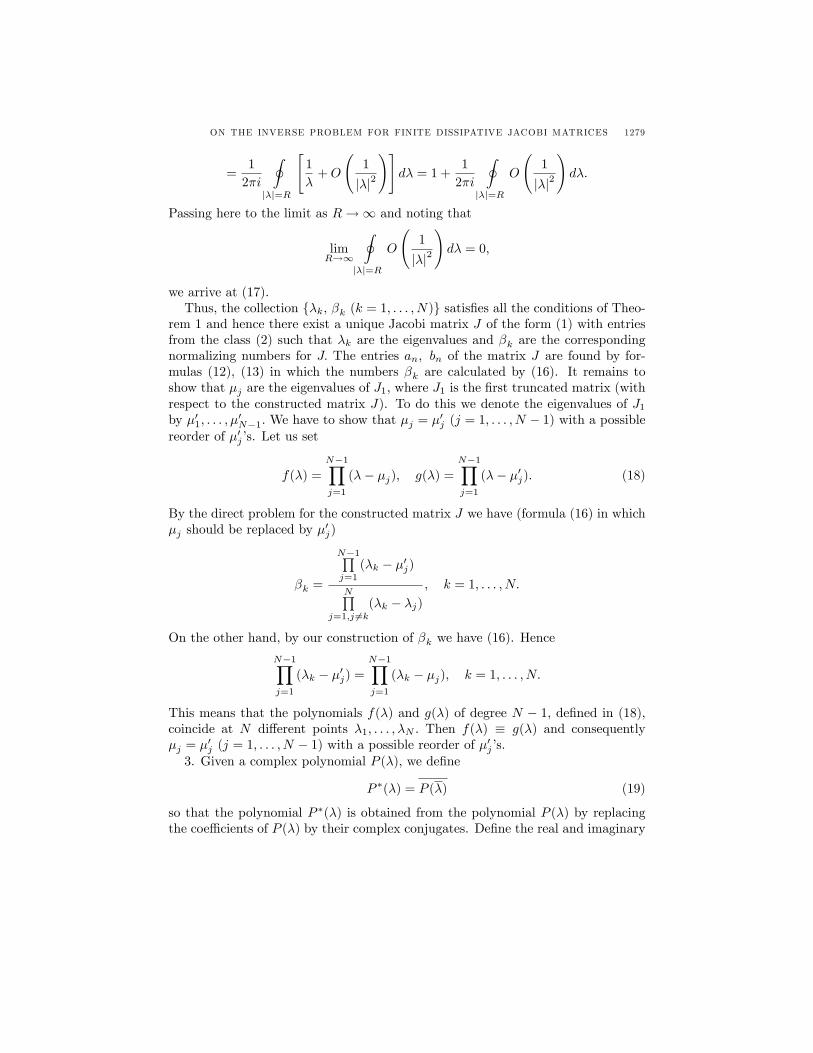
=1

2πi

∮|λ|=R

[1

λ+O

(1

|λ|2

)]dλ = 1 +

1

2πi

∮|λ|=R

O

(1

|λ|2

)dλ.

Passing here to the limit as R→∞ and noting that

limR→∞

∮|λ|=R

O

(1

|λ|2

)dλ = 0,

we arrive at (17).Thus, the collection {λk, βk (k = 1, . . . , N)} satisfies all the conditions of Theo-

rem 1 and hence there exist a unique Jacobi matrix J of the form (1) with entriesfrom the class (2) such that λk are the eigenvalues and βk are the correspondingnormalizing numbers for J. The entries an, bn of the matrix J are found by for-mulas (12), (13) in which the numbers βk are calculated by (16). It remains toshow that µj are the eigenvalues of J1, where J1 is the first truncated matrix (withrespect to the constructed matrix J). To do this we denote the eigenvalues of J1by µ′1, . . . , µ

′N−1. We have to show that µj = µ′j (j = 1, . . . , N − 1) with a possible

reorder of µ′j’s. Let us set

f(λ) =

N−1∏j=1

(λ− µj), g(λ) =

N−1∏j=1

(λ− µ′j). (18)

By the direct problem for the constructed matrix J we have (formula (16) in whichµj should be replaced by µ

′j)

βk =

N−1∏j=1

(λk − µ′j)

N∏j=1,j 6=k

(λk − λj), k = 1, . . . , N.

On the other hand, by our construction of βk we have (16). Hence

N−1∏j=1

(λk − µ′j) =

N−1∏j=1

(λk − µj), k = 1, . . . , N.

This means that the polynomials f(λ) and g(λ) of degree N − 1, defined in (18),coincide at N different points λ1, . . . , λN . Then f(λ) ≡ g(λ) and consequentlyµj = µ′j (j = 1, . . . , N − 1) with a possible reorder of µ′j’s.3. Given a complex polynomial P (λ), we define

P ∗(λ) = P (λ) (19)

so that the polynomial P ∗(λ) is obtained from the polynomial P (λ) by replacingthe coeffi cients of P (λ) by their complex conjugates. Define the real and imaginary

1280 EBRU ERGUN

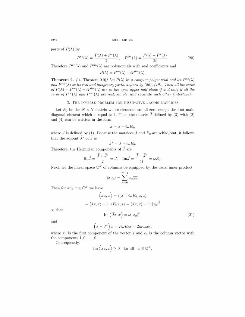
parts of P (λ) by

P re(λ) =P (λ) + P ∗(λ)

2, P im(λ) =

P (λ)− P ∗(λ)

2i. (20)

Therefore P re(λ) and P im(λ) are polynomials with real coeffi cients and

P (λ) = P re(λ) + iP im(λ).

Theorem 2. ([4, Theorem 9.9]) Let P (λ) be a complex polynomial and let P re(λ)and P im(λ) be its real and imaginary parts, defined by (20), (19). Then all the zerosof P (λ) = P re(λ) + iP im(λ) are in the open upper half-plane if and only if all thezeros of P re(λ) and P im(λ) are real, simple, and separate each other (interlace).

3. The inverse problem for dissipative Jacobi matrices

Let E0 be the N × N matrix whose elements are all zero except the first maindiagonal element which is equal to 1. Then the matrix J defined by (3) with (2)and (4) can be written in the form

J = J + iωE0,

where J is defined by (1). Because the matrices J and E0 are selfadjoint, it followsthat the adjoint J∗ of J is

J∗ = J − iωE0.Therefore, the Hermitian components of J are

ReJ =J + J∗

2= J, ImJ =

J − J∗

2I= ωE0.

Next, let the linear space CN of columns be equipped by the usual inner product

〈x, y〉 =

N−1∑n=0

xnyn.

Then for any x ∈ CN we have⟨Jx, x

⟩= 〈(J + iωE0)x, x〉

= 〈Jx, x〉+ iω 〈E0x, x〉 = 〈Jx, x〉+ iω |x0|2

so thatIm⟨Jx, x

⟩= ω |x0|2 , (21)

and (J − J∗

)x = 2iωE0x = 2iωx0e0,

where x0 is the first component of the vector x and e0 is the column vector withthe components 1, 0, . . . , 0.Consequently,

Im⟨Jx, x

⟩≥ 0 for all x ∈ CN ,


ran(J − J∗

)= {αe0 : α ∈ C},

so that, J is a dissipative Jacobi matrix with a rank-one imaginary part.

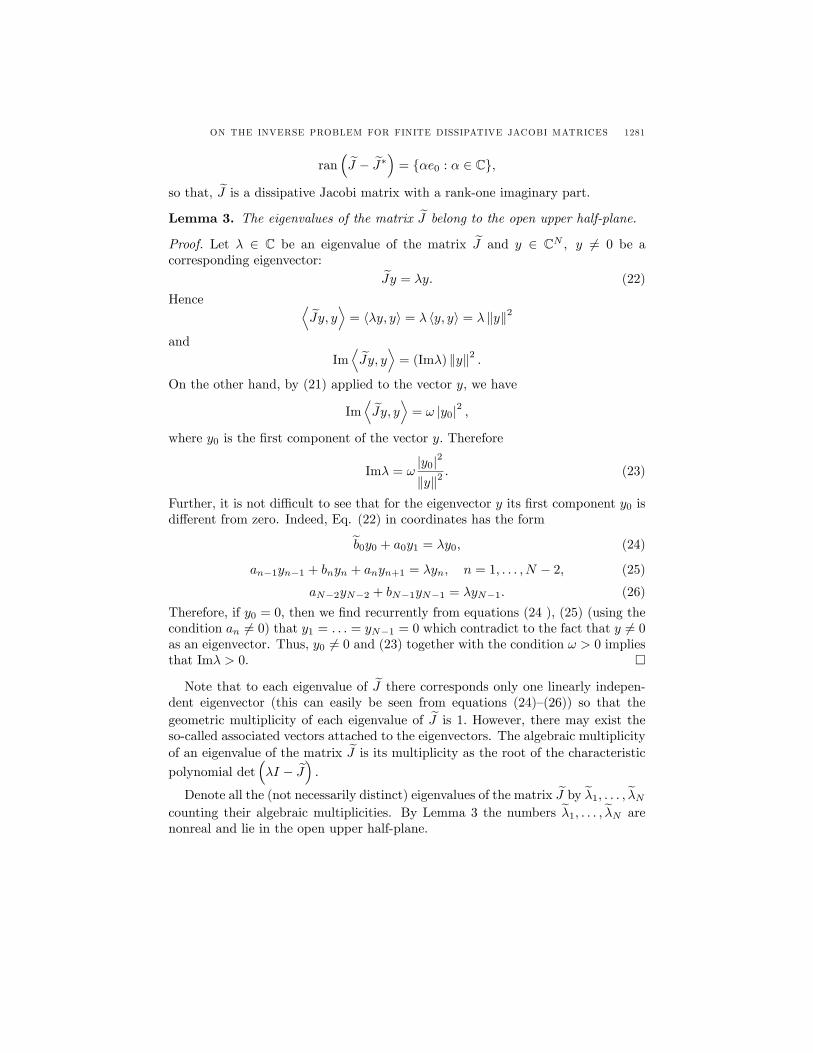
Lemma 3. The eigenvalues of the matrix J belong to the open upper half-plane.

Proof. Let λ ∈ C be an eigenvalue of the matrix J and y ∈ CN , y 6= 0 be acorresponding eigenvector:

Jy = λy. (22)

Hence ⟨Jy, y

⟩= 〈λy, y〉 = λ 〈y, y〉 = λ ‖y‖2

andIm⟨Jy, y

⟩= (Imλ) ‖y‖2 .

On the other hand, by (21) applied to the vector y, we have

Im⟨Jy, y

⟩= ω |y0|2 ,

where y0 is the first component of the vector y. Therefore

Imλ = ω|y0|2

‖y‖2. (23)

Further, it is not diffi cult to see that for the eigenvector y its first component y0 isdifferent from zero. Indeed, Eq. (22) in coordinates has the form

b0y0 + a0y1 = λy0, (24)

an−1yn−1 + bnyn + anyn+1 = λyn, n = 1, . . . , N − 2, (25)

aN−2yN−2 + bN−1yN−1 = λyN−1. (26)

Therefore, if y0 = 0, then we find recurrently from equations (24 ), (25) (using thecondition an 6= 0) that y1 = . . . = yN−1 = 0 which contradict to the fact that y 6= 0as an eigenvector. Thus, y0 6= 0 and (23) together with the condition ω > 0 impliesthat Imλ > 0. �

Note that to each eigenvalue of J there corresponds only one linearly indepen-dent eigenvector (this can easily be seen from equations (24)—(26)) so that thegeometric multiplicity of each eigenvalue of J is 1. However, there may exist theso-called associated vectors attached to the eigenvectors. The algebraic multiplicityof an eigenvalue of the matrix J is its multiplicity as the root of the characteristic

polynomial det(λI − J

).

Denote all the (not necessarily distinct) eigenvalues of the matrix J by λ1, . . . , λNcounting their algebraic multiplicities. By Lemma 3 the numbers λ1, . . . , λN arenonreal and lie in the open upper half-plane.

1282 EBRU ERGUN

Lemma 4. The equalityN∑j=1

Imλj = ω (27)

holds, where ω > 0 is taken from (4).

Proof. For any matrix A = [ajk]Nj,k=1 the spectral trace of A equals its matrix trace:If z1, . . . , zN are all the eigenvalues (counting their algebraic multiplicities) of A,then

N∑j=1

zj =

N∑j=1

ajj .

Therefore we can write, for the matrix J ,N∑j=1

λj = b0 + b1 + . . .+ bN−1,

where b0 has the form (4). Taking here the imaginary part we get (27). �

The following simple lemma is crucial in our solving the inverse spectral problemfor the matrix J .

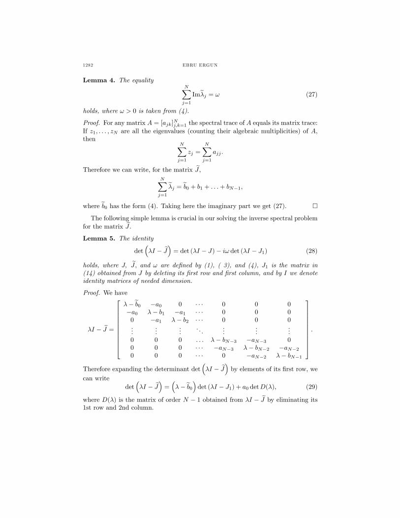
Lemma 5. The identity

det(λI − J

)= det (λI − J)− iω det (λI − J1) (28)

holds, where J, J , and ω are defined by (1), ( 3), and (4), J1 is the matrix in(14) obtained from J by deleting its first row and first column, and by I we denoteidentity matrices of needed dimension.

Proof. We have

λI − J =

λ− b0 −a0 0 · · · 0 0 0−a0 λ− b1 −a1 · · · 0 0 0

0 −a1 λ− b2 · · · 0 0 0...

......

. . ....

......

0 0 0 . . . λ− bN−3 −aN−3 00 0 0 · · · −aN−3 λ− bN−2 −aN−20 0 0 · · · 0 −aN−2 λ− bN−1

.

Therefore expanding the determinant det(λI − J

)by elements of its first row, we

can writedet(λI − J

)=(λ− b0

)det (λI − J1) + a0 detD(λ), (29)

where D(λ) is the matrix of order N − 1 obtained from λI − J by eliminating its1st row and 2nd column.


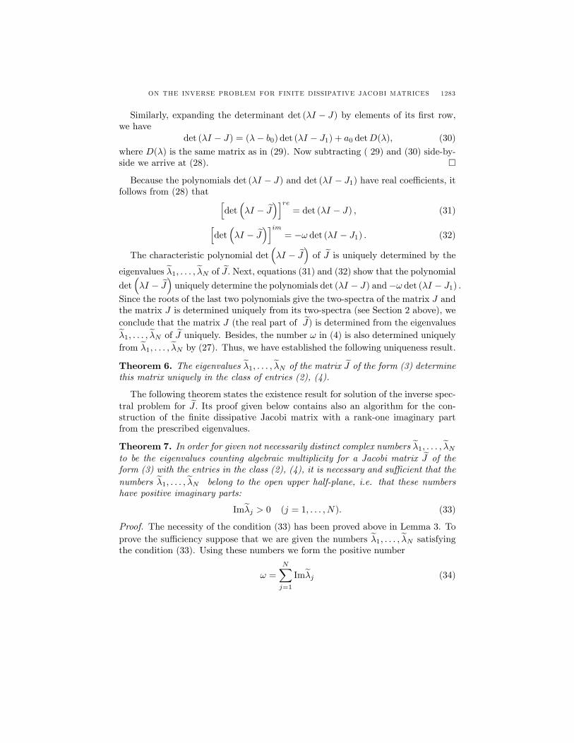
Similarly, expanding the determinant det (λI − J) by elements of its first row,we have

det (λI − J) = (λ− b0) det (λI − J1) + a0 detD(λ), (30)

where D(λ) is the same matrix as in (29). Now subtracting ( 29) and (30) side-by-side we arrive at (28). �

Because the polynomials det (λI − J) and det (λI − J1) have real coeffi cients, itfollows from (28) that [

det(λI − J

)]re= det (λI − J) , (31)[

det(λI − J

)]im= −ω det (λI − J1) . (32)

The characteristic polynomial det(λI − J

)of J is uniquely determined by the

eigenvalues λ1, . . . , λN of J . Next, equations (31) and (32) show that the polynomial

det(λI − J

)uniquely determine the polynomials det (λI − J) and−ω det (λI − J1) .

Since the roots of the last two polynomials give the two-spectra of the matrix J andthe matrix J is determined uniquely from its two-spectra (see Section 2 above), weconclude that the matrix J (the real part of J) is determined from the eigenvaluesλ1, . . . , λN of J uniquely. Besides, the number ω in (4) is also determined uniquelyfrom λ1, . . . , λN by (27). Thus, we have established the following uniqueness result.

Theorem 6. The eigenvalues λ1, . . . , λN of the matrix J of the form (3) determinethis matrix uniquely in the class of entries (2), (4).

The following theorem states the existence result for solution of the inverse spec-tral problem for J . Its proof given below contains also an algorithm for the con-struction of the finite dissipative Jacobi matrix with a rank-one imaginary partfrom the prescribed eigenvalues.

Theorem 7. In order for given not necessarily distinct complex numbers λ1, . . . , λNto be the eigenvalues counting algebraic multiplicity for a Jacobi matrix J of theform (3) with the entries in the class (2), (4), it is necessary and suffi cient that thenumbers λ1, . . . , λN belong to the open upper half-plane, i.e. that these numbershave positive imaginary parts:

Imλj > 0 (j = 1, . . . , N). (33)

Proof. The necessity of the condition (33) has been proved above in Lemma 3. Toprove the suffi ciency suppose that we are given the numbers λ1, . . . , λN satisfyingthe condition (33). Using these numbers we form the positive number

ω =

N∑j=1

Imλj (34)

1284 EBRU ERGUN

and the polynomial

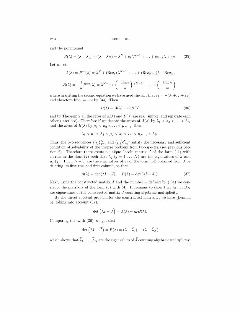
P (λ) = (λ− λ1) · · · (λ− λN ) = λN + c1λN−1 + . . .+ cN−1λ+ cN . (35)

Let us set

A(λ) = P re(λ) = λN + (Rec1)λN−1 + . . .+ (RecN−1)λ+ RecN ,

B(λ) = − 1

ωP im(λ) = λN−1 +

(− Imc2

ω

)λN−2 + . . .+

(− ImcN

ω

),

where in writing the second equation we have used the fact that c1 = −(λ1+. . .+λN )and therefore Imc1 = −ω by (34). Then

P (λ) = A(λ)− iωB(λ) (36)

and by Theorem 2 all the zeros of A(λ) and B(λ) are real, simple, and separate eachother (interlace). Therefore if we denote the zeros of A(λ) by λ1 < λ2 < . . . < λNand the zeros of B(λ) by µ1 < µ2 < . . . < µN−1, then

λ1 < µ1 < λ2 < µ2 < λ3 < . . . < µN−1 < λN .

Thus, the two sequences {λj}Nj=1 and {µj}N−1j=1 satisfy the necessary and suffi cientcondition of solvability of the inverse problem from two-spectra (see previous Sec-tion 2). Therefore there exists a unique Jacobi matrix J of the form ( 1) withentries in the class (2) such that λj (j = 1, . . . , N) are the eigenvalues of J andµj (j = 1, . . . , N − 1) are the eigenvalues of J1 of the form (14) obtained from J bydeleting its first row and first column, so that

A(λ) = det (λI − J) , B(λ) = det (λI − J1) . (37)

Next, using the constructed matrix J and the number ω defined by ( 34) we con-struct the matrix J of the form (3) with (4). It remains to show that λ1, . . . , λNare eigenvalues of the constructed matrix J counting algebraic multiplicity.By the direct spectral problem for the constructed matrix J , we have (Lemma

5), taking into account (37),

det(λI − J

)= A(λ)− iωB(λ).

Comparing this with (36), we get that

det(λI − J

)= P (λ) = (λ− λ1) · · · (λ− λN )

which shows that λ1, . . . , λN are the eigenvalues of J counting algebraic multiplicity.�


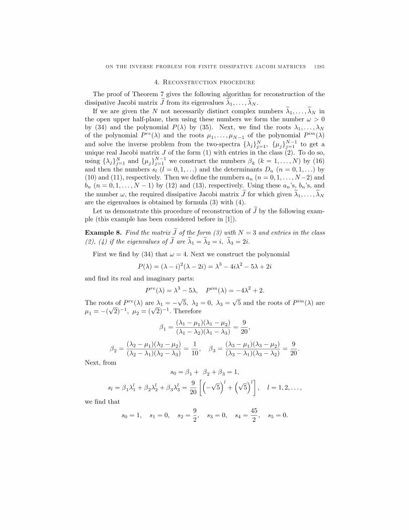
4. Reconstruction procedure

The proof of Theorem 7 gives the following algorithm for reconstruction of thedissipative Jacobi matrix J from its eigenvalues λ1, . . . , λN .If we are given the N not necessarily distinct complex numbers λ1, . . . , λN in

the open upper half-plane, then using these numbers we form the number ω > 0by (34) and the polynomial P (λ) by (35). Next, we find the roots λ1, . . . , λNof the polynomial P re(λ) and the roots µ1, . . . , µN−1 of the polynomial P

im(λ)

and solve the inverse problem from the two-spectra {λj}Nj=1, {µj}N−1j=1 to get aunique real Jacobi matrix J of the form (1) with entries in the class (2). To do so,using {λj}Nj=1 and {µj}N−1j=1 we construct the numbers βk (k = 1, . . . , N) by (16)and then the numbers sl (l = 0, 1, . . .) and the determinants Dn (n = 0, 1, . . .) by(10) and (11), respectively. Then we define the numbers an (n = 0, 1, . . . , N−2) andbn (n = 0, 1, . . . , N − 1) by (12) and (13), respectively. Using these an’s, bn’s, andthe number ω, the required dissipative Jacobi matrix J for which given λ1, . . . , λNare the eigenvalues is obtained by formula (3) with (4).Let us demonstrate this procedure of reconstruction of J by the following exam-

ple (this example has been considered before in [1]).

Example 8. Find the matrix J of the form (3) with N = 3 and entries in the class(2), (4) if the eigenvalues of J are λ1 = λ2 = i, λ3 = 2i.

First we find by (34) that ω = 4. Next we construct the polynomial

P (λ) = (λ− i)2(λ− 2i) = λ3 − 4iλ2 − 5λ+ 2i

and find its real and imaginary parts:

P re(λ) = λ3 − 5λ, P im(λ) = −4λ2 + 2.

The roots of P re(λ) are λ1 = −√

5, λ2 = 0, λ3 =√

5 and the roots of P im(λ) areµ1 = −(

√2)−1, µ2 = (

√2)−1. Therefore

β1 =(λ1 − µ1)(λ1 − µ2)(λ1 − λ2)(λ1 − λ3)

=9

20,

β2 =(λ2 − µ1)(λ2 − µ2)(λ2 − λ1)(λ2 − λ3)

=1

10, β3 =

(λ3 − µ1)(λ3 − µ2)(λ3 − λ1)(λ3 − λ2)

=9

20.

Next, froms0 = β1 + β2 + β3 = 1,

sl = β1λl1 + β2λ

l2 + β3λ

l3 =

9

20

[(−√

5)l

+(√

5)l]

, l = 1, 2, . . . ,

we find that

s0 = 1, s1 = 0, s2 =9

2, s3 = 0, s4 =

45

2, s5 = 0.

1286 EBRU ERGUN

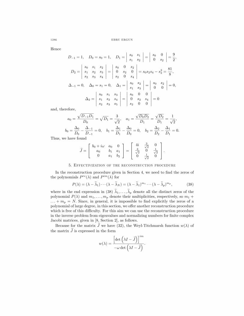
Hence

D−1 = 1, D0 = s0 = 1, D1 =

∣∣∣∣ s0 s1s1 s2

∣∣∣∣ =

∣∣∣∣ s0 00 s2

∣∣∣∣ =9

2,

D2 =

∣∣∣∣∣∣s0 s1 s2s1 s2 s3s2 s3 s4

∣∣∣∣∣∣ =

∣∣∣∣∣∣s0 0 s20 s2 0s2 0 s4

∣∣∣∣∣∣ = s0s2s4 − s32 =81

8,

∆−1 = 0, ∆0 = s1 = 0, ∆1 =

∣∣∣∣ s0 s2s1 s3

∣∣∣∣ =

∣∣∣∣ s0 s20 0

∣∣∣∣ = 0,

∆2 =

∣∣∣∣∣∣s0 s1 s3s1 s2 s4s2 s3 s5

∣∣∣∣∣∣ =

∣∣∣∣∣∣s0 0 00 s2 s4s2 0 0

∣∣∣∣∣∣ = 0

and, therefore,

a0 =

√D−1D1

D0=√D1 =

3√2, a1 =

√D0D2

D1=

√D2

D1=

1√2,

b0 =∆0

D0− ∆−1D−1

= 0, b1 =∆1

D1− ∆0

D0= 0, b2 =

∆2

D2− ∆1

D1= 0.

Thus, we have found

J =

b0 + iω a0 0a0 b1 a10 a1 b2

=

4i 3√2

03√2

0 1√2

0 1√2

0

.5. Effectivization of the reconstruction procedure

In the reconstruction procedure given in Section 4, we need to find the zeros ofthe polynomials P re(λ) and P im(λ) for

P (λ) = (λ− λ1) · · · (λ− λN ) = (λ− λ1)m1 · · · (λ− λp)mp , (38)

where in the end expression in (38) λ1, . . . , λp denote all the distinct zeros of thepolynomial P (λ) and m1, . . . ,mp denote their multiplicities, respectively, so m1 +. . . + mp = N. Since, in general, it is impossible to find explicitly the zeros of apolynomial of large degree, in this section, we offer another reconstruction procedurewhich is free of this diffi culty. For this aim we can use the reconstruction procedurein the inverse problem from eigenvalues and normalizing numbers for finite complexJacobi matrices, given in [8, Section 2], as follows.Because for the matrix J we have (32), the Weyl-Titchmarsh function w(λ) of

the matrix J is expressed in the form

w(λ) =

[det(λI − J

)]im−ω det

(λI − J

) .


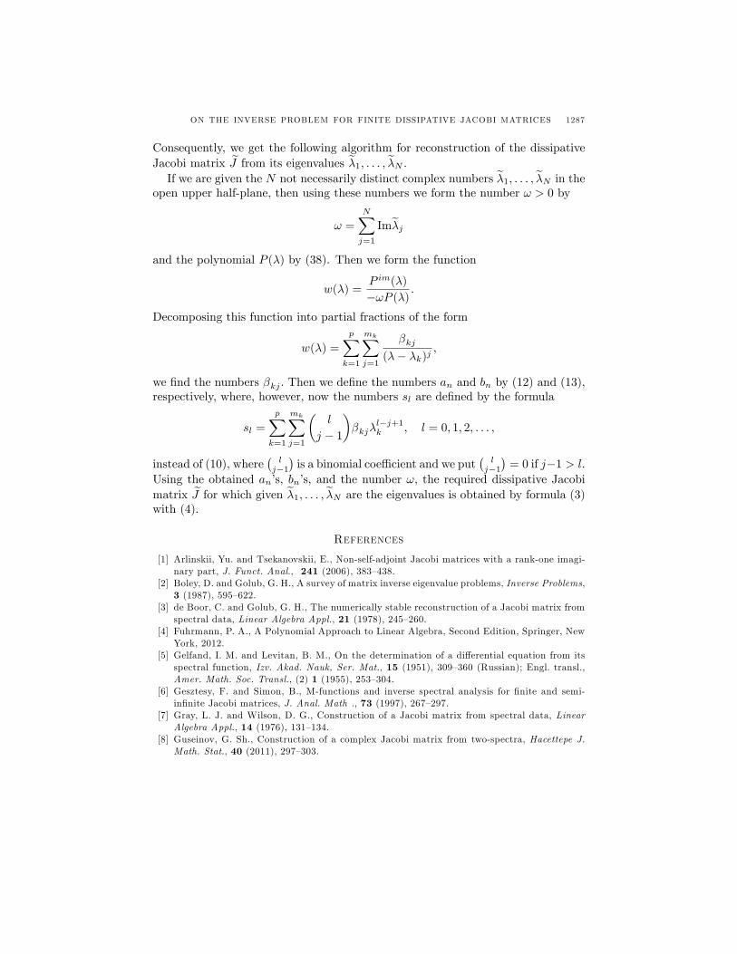
Consequently, we get the following algorithm for reconstruction of the dissipativeJacobi matrix J from its eigenvalues λ1, . . . , λN .If we are given the N not necessarily distinct complex numbers λ1, . . . , λN in the

open upper half-plane, then using these numbers we form the number ω > 0 by

ω =

N∑j=1

Imλj

and the polynomial P (λ) by (38). Then we form the function

w(λ) =P im(λ)

−ωP (λ).

Decomposing this function into partial fractions of the form

w(λ) =

p∑k=1

mk∑j=1

βkj(λ− λk)j

,

we find the numbers βkj . Then we define the numbers an and bn by (12) and (13),respectively, where, however, now the numbers sl are defined by the formula

sl =

p∑k=1

mk∑j=1

(l

j − 1

)βkjλ

l−j+1k , l = 0, 1, 2, . . . ,

instead of (10), where(l

j−1)is a binomial coeffi cient and we put

(l

j−1)

= 0 if j−1 > l.

Using the obtained an’s, bn’s, and the number ω, the required dissipative Jacobimatrix J for which given λ1, . . . , λN are the eigenvalues is obtained by formula (3)with (4).

References

[1] Arlinskii, Yu. and Tsekanovskii, E., Non-self-adjoint Jacobi matrices with a rank-one imagi-nary part, J. Funct. Anal., 241 (2006), 383—438.

[2] Boley, D. and Golub, G. H., A survey of matrix inverse eigenvalue problems, Inverse Problems,3 (1987), 595—622.

[3] de Boor, C. and Golub, G. H., The numerically stable reconstruction of a Jacobi matrix fromspectral data, Linear Algebra Appl., 21 (1978), 245—260.

[4] Fuhrmann, P. A., A Polynomial Approach to Linear Algebra, Second Edition, Springer, NewYork, 2012.

[5] Gelfand, I. M. and Levitan, B. M., On the determination of a differential equation from itsspectral function, Izv. Akad. Nauk, Ser. Mat., 15 (1951), 309—360 (Russian); Engl. transl.,Amer. Math. Soc. Transl., (2) 1 (1955), 253—304.

[6] Gesztesy, F. and Simon, B., M-functions and inverse spectral analysis for finite and semi-infinite Jacobi matrices, J. Anal. Math ., 73 (1997), 267—297.

[7] Gray, L. J. and Wilson, D. G., Construction of a Jacobi matrix from spectral data, LinearAlgebra Appl., 14 (1976), 131—134.

[8] Guseinov, G. Sh., Construction of a complex Jacobi matrix from two-spectra, Hacettepe J.Math. Stat., 40 (2011), 297—303.

1288 EBRU ERGUN

[9] Guseinov, G. Sh., On an inverse problem for two spectra of finite Jacobi matrices, Appl.Math. Comput., 218 (2012), 7573—7589.

[10] Guseinov, G. Sh., On a discrete inverse problem for two spectra, Discrete Dynamics in Natureand Society, 2012 (2012), Article ID 956407, 14 pages.

[11] Hald, O. H., Inverse eigenvalue problems for Jacobi matrices, Linear Algebra Appl., 14 (1976),63—85.

[12] Hochstadt, H., On some inverse problems in matrix theory, Arch. Math., 18 (1967), 201—207.[13] Hochstadt, H., On construction of a Jacobi matrix from spectral data, Linear Algebra Appl.,

8 (1974), 435—446.[14] Huseynov, A. and Guseinov, G. Sh., Solution of the finite complex Toda lattice by the method

of inverse spectral problem, Appl. Math. Comput., 219 (2013), 5550—5563.[15] Teschl, G., Jacobi Operators and Completely Integrable Nonlinear Lattices, vol. 72 of Math-

ematical Surveys and Monographs, American Mathematical Society, 2000.[16] Ergun, E. and Huseynov, A., On an Inverse Problem for a Quadratic Eigenvalue Problem,

Int. J. Difference Equ., vol. 12, 1 (2017), 13—26.

Current address : Ebru ERGUN: Department of Mathematics, Karabuk University, 78050Karabuk, TURKEY.

E-mail address : [email protected] Address: http://orcid.org/0000-0003-4873-6191

on the inverse problem for finite dissipative jacobi matrices ...

Documents