On the influence of cooling and heating processes on Parker ...

Mon. Not. R. Astron. Soc. 368, 759–768 (2006) doi:10.1111/j.1365-2966.2006.10142.x

On the influence of cooling and heating processes on Parker instability

R. Kosinski� and M. HanaszTorun Centre for Astronomy, Nicolaus Copernicus University, Piwnice/Torun, PL-87148, Poland

Accepted 2006 February 2. Received 2006 January 25; in original form 2005 October 19

ABSTRACT

We study Parker instability (PI) operating in a non-adiabatic, gravitationally stratified, in-terstellar medium. We discuss models with two kinds of heating mechanisms. The first oneresults from photoionization models. The other, relying on supplemental sources, has beenpostulated by Reynolds, Haffner & Tufte. The cooling rate, corresponding to radiative losses,is an approximation to the one given by Dalgarno & McCray. An unperturbed state of thesystem represents a magnetohydrostatic and thermal equilibrium. We perform linear stabilityanalysis by solving the boundary value problem. We find that the maximum growth rate of PIrises for increasing magnitudes of non-adiabatic effects. In the pure photoionization model,the maximum growth rate of the general non-adiabatic case coincides with the isothermallimit. Adding other sources of heat leads to a maximum growth rate that is larger than the onecorresponding to the isothermal limit. We find that the influence of the supplemental heatingon PI also leads to a decrease in temperature in magnetic valleys. Finally, we conclude that theinitial gas cooling due to the action of PI may promote a subsequent onset of thermal instabilityin magnetic valleys and formation of giant molecular clouds.

Key words: magnetic fields – MHD – ISM: kinematics and dynamics – galaxies: ISM.

1 I N T RO D U C T I O N

Parker instability (PI; Parker 1966, 1967a,b) is induced by the buoy-ancy of the magnetic field and cosmic rays. It is considered as aprocess significantly influencing the structure and dynamics of theinterstellar medium (ISM) and is supposed to play an importantrole in the formation of giant molecular cloud (GMC) complexes(Mouschovias, Shu & Woodward 1974; Blitz & Shu 1980).

Linear analysis of PI is usually performed for a simple model ofthe ISM, which initially remains in a state of magnetohydrostaticequilibrium in an external vertical gravitational field. The ISM isapproximated by a single gas phase, which is threaded by a regularmagnetic field, and penetrated by diffuse cosmic rays.

Numerous authors have investigated different modifications to thestandard set-up: the effects of linear and realistic gravitational fielddistributions (Giz & Shu 1993; Kim, Hong & Ryu 1997); rotationaland inertial forces (Shu 1974; Foglizzo & Tagger 1994; Hanasz,Otmianowska-Mazur & Lesch 2002); locally injected cosmic rays(Hanasz & Lesch 2000, 2003; Kuwabara, Nakamura & Ko 2004); themulticomponent nature of the ISM (Santillan et al. 2000); irregular,random components of the magnetic field (Parker & Jokipii 2000;Kim & Ryu 2001); and effects of spiral arms (Franco et al. 2002). Themain assumption made in these studies is an adiabatic or isothermalmagnetohydrodynamic (MHD) evolution of the interstellar gas.

�E-mail: [email protected]

Kim et al. (1998) investigated the issue of cloud formation by PIby means of numerical simulations. They found that ‘the maximumdensity enhancement factor in the scale of giant molecular clouds(GMC) is only ∼2’. They concluded that ‘it is difficult to regard PIalone as the formation mechanism of GMCs’.

In response to this statement, Parker & Jokipii (2000) suggestedthat one should ‘recognize the tendency of the interstellar gas tem-perature in thermal equilibrium to decline with increasing density,so that δ p/p � γ δρ/ρ, where γ < 1, introducing the thermal insta-bility (Parker 1953a,b) responsible for the enormous gas densitiesin the interstellar molecular clouds’.

Thermal instability (TI) has been investigated by Field (1965)who formulated the instability criteria for a wide variety of astro-physical circumstances. In order to relate the analysis of TI to theISM, one has to specify the relevant non-adiabatic (cooling andheating) processes.

Typical heating sources are O- and B-type stars, which interactwith the interstellar matter mainly by their dilute radiation field(Domgorgen & Mathis 1994). Ultraviolet (UV) photons from thesestars dissociate molecules on clouds surfaces, ionize atoms and si-multaneously heat up surrounding interstellar space to temperaturesof about 104 K in the galactic disc.

The pure photoionization models appeared to be insufficient to ex-plain the following observational fact: the gas temperature changesinversely with the density of the diffuse interstellar gas and risesfrom ∼7000 K at the galactic mid-plane to about 12 000 K at thealtitude of 2 kpc above the mid-plane. Thus, there must exist an addi-tional heat source that dominates ionization heating at low densities

C© 2006 The Authors. Journal compilation C© 2006 RAS

Dow

nloaded from https://academ

ic.oup.com/m

nras/article/368/2/759/985050 by guest on 22 June 2022

760 R. Kosinski and M. Hanasz

(Reynolds et al. 1999 and references therein). Such heat sources inthe warm ISM may include photoelectric heating by dust, the dis-sipation of interstellar turbulence, Coulomb collisions with cosmicrays, which are proportional to density in first power (Skibo, Ra-maty & Purcell 1996), and magnetic reconnection, which may benearly independent of density (Goncalves, Jatenco-Pereira & Opher1993).

On the other hand, the partially ionized gas cools down because ofthe conversion of the kinetic particle energy into radiation throughcollisional processes (Dalgarno & McCray 1972). The cooling canbe efficient, if gas is optically thin for radiated photons. In the inter-stellar matter with cosmic abundances, the cooling at high tempera-tures proceeds through excitation of neutral and ionized constituentsas a result of collisions with free electrons. At lower temperatures,the collisional excitation of fine levels is important. The coolingefficiency depends strongly on the chemical composition of the in-terstellar gas. An imbalance of heating and cooling may lead to TIin gas, a phenomenon described in detail by Field (1965).

The influence of non-adiabatic processes on PI was previouslyinvestigated by Ames (1973). The author concluded that addingthermal effects reduces the scale of unstable perturbations and in-creases the PI growth rate above the adiabatic limit.

In this paper, we present a linear analysis of PI influenced bythe additional heat sources proposed by Reynolds, Haffner & Tufte(1999). For simplicity, we neglect the cosmic ray component of theISM. We take into account two models of the magnetohydrostaticand thermal disc equilibrium. The first is based on photoionizationheating only, and the second incorporates supplemental heat sourcesfollowing Reynolds et al. (1999).

The plan of the paper is as follows. In Section 2, we describethe initial atmosphere incorporating the non-adiabatic processesand perform a linear analysis of PI under the influence of cool-ing and heating processes. We derive the dispersion relation for PI,which is generalized for the presence of non-adiabatic processes. InSection 3, we numerically analyse the dispersion relation for thetwo models mentioned above. We provide a physical interpretationof our results in Section 4 and conclude in Section 5.

2 L I N E A R S TA B I L I T Y A NA LY S I S

2.1 Basic equations

In the following considerations, we apply the standard non-adiabaticMHD equations together with the ideal gas equation of state:

∂ρ

∂t+ ∇ · (ρv) = 0, (1)

ργ

γ − 1

(∂

∂t+ v · ∇

)(Pργ

)= � − n2�(T ), (2)

∂v

∂t+ (v · ∇)v = g − 1

ρ∇

(P + B2

8π

)+ 1

4πρ(B · ∇)B, (3)

∂B

∂t= ∇ × (v× B), (4)

P = nkBT , (5)

where γ is the ratio of the specific heats, n ≡ ρ/mH is the numberdensity, � is the heating rate per unit volume, hereafter referred to asthe heating function, and � is the cooling function. Other symbolshave their usual meaning.

Figure 1. The Dalgarno–McCray cooling function (solid line) along withits analytic approximation (dashed line) and a modelled curve for higherfractional ionization, applied in the paper (dotted line). A circle on the dottedline marks the critical temperature T crit for the onset of TI in model M2.

2.2 Cooling and heating functions

The cooling function for a realistic ISM has been described byDalgarno & McCray (1972). In order to study the qualitative ef-fects of the non-adiabatic processes on PI, we apply the followinganalytic formula that approximates the Dalgarno–McCray coolingfunction in the temperature range 1000 K � T � 14 000 K, for frac-tional ionization (defined as the ratio of electron to proton numberdensities) � 0.1:

�(T ) = LC1T ε1 + LC2 exp

[− c

(T − 100)ε2

]. (6)

Values of constants in the above formula are L C1 = 4.4 × 10−67 ergcm3 s−1 K−10.73, ε1 = 10.73, L C2 = 7.2 × 10−25 erg cm3 s−1, ε2 =0.6, c = 40.0. In Fig. 1, we plot the original Dalgarno–McCray cool-ing function for fractional ionization ∼0.1 (full line) together withtwo variants of our own approximation: one for the same fractionalionization (dashed line) and one for a larger fractional ionization(dotted line). The value of L C2 controls the cooling curve plateaulevel. We adopt L C2 = 1.6 × 10−24 erg cm3 s−1 in order to model thethermal properties of the warm ionized medium in our calculations.In the present paper, we shall not involve the gas fraction warmerthan the mentioned 14 000 K; therefore, we neglect the differencesof our approximation with respect to the original Dalgarno–McCraycooling function at large temperatures.

Following Reynolds et al. (1999), we adopt the heating functionof the form

� = �UV + �1, (7)

where

�UV = n2G0, �1 = nG1, (8)

and G 0, G 1 are constants. As mentioned already, the supplemen-tal heat sources may result from photoelectric heating by dust, thedissipation of interstellar turbulence or Coulomb collisions with cos-mic rays. The corresponding additional source terms in the energyequation are proportional to n through �1. In this paper, we neglectanother heating term discussed by Reynolds et al. (1999), which isindependent of n.

We define the following two heating models that are to be exam-ined separately in the forthcoming analysis. Model M1 representsa pure photoionization heating defined by G 0 = �0 = �(T 0), for

C© 2006 The Authors. Journal compilation C© 2006 RAS, MNRAS 368, 759–768

Dow


ic.oup.com/m


Parker instability 761

the initial constant temperature T 0 and G 1 = 0. Model M2 repre-sents the photoionization together with supplemental heat sourcesspecified by constants G 0 = 1 × 10−24 erg cm3 s−1 and G 1 = 1 ×10−25 erg s−1, adopted from Reynolds et al. (1999).

2.3 Conditions for thermal instability

The presence of cooling and heating effects operating in a gaseousmedium may lead to TI (Parker 1953a,b; Field 1965). TI sets onwhen a negative temperature perturbation of a medium (in thermalequilibrium) leads to an excess of cooling over heating, or a positivetemperature perturbation leads to an excess of heating over cooling.This means that, in the first case, a blob of gas, displaced towardslower temperatures cools down and becomes denser and denser,under the pressure of the surrounding gas, until it reaches anotherstable thermal equilibrium state.

The criterion for TI derived by Field (1965) is(∂L∂S

)A

< 0, (9)

where

L = �

n− n� (10)

is defined as energy gain minus energy losses per gram of materialper second, S denotes entropy of the material and A is a thermody-namic variable, which remains constant while density and temper-ature undergo dynamical variations.

Field’s criterion for an isobaric perturbation can be written as

∂

∂T

(�

n− n�

)n

− n0

T0

∂

∂n

(�

n− n�

)T

> 0. (11)

In the present case of the cooling and heating given by equations(6) and (7) respectively, the criterion reduces to the following form:

F(T ) = Td�

dT− κ(� − G0) < 0, (12)

where κ = 0 for model M1 and κ = 1 for model M2.One can note that model M1 is thermally stable in the considered

temperature range, because the cooling function is monotonicallygrowing with T . On the other hand, model M2 appears to be ther-mally unstable for temperatures T lower than T crit, and stable aboveT crit, at which F(T crit) = 0. For the present choice of cooling andheating parameters of model M2, T crit � 5840 K.

2.4 Unperturbed equilibrium state

We first construct the unperturbed magnetohydrostatic and thermalequilibrium state. We assume that galactic disc permeated by thehorizontal magnetic field B0 = B 0(z) e y is stratified by a uniformvertical gravity g = −gz ez , where gz = 2.0 × 10−9 cm s−2. Follow-ing Parker (1966, 1967a,b), we assume that the equilibrium magneticand gas pressures fulfill the relation

Pmag = αP0, (13)

where α is a constant of the order of 1. In the present considerations,we adopt α = 1. The magnetohydrostatic equilibrium condition canbe written as

(1 + α)dP0

dz= −ρ0gz, (14)

where the vertical distributions of pressure P 0(z), density ρ 0(z) andtemperature T 0(z) are related by the equation of state

P0(z) = kBρ0(z)

mHT0(z). (15)

The thermal equilibrium means balance between heating andcooling

n20(z)�0(z) = �0(z), (16)

where �0(z) ≡ �[T 0(z)] (see equation 6) and �0(z) is specifiedbelow, separately for models M1 and M2.

In model M1, the heating and cooling balance implies

�0A(z) = n0(z)2G0 = n0(z)2�0(z), (17)

where �0(z) = const with assumed T 0(z) = T 0 = const as thetemperature of the disc. The magnetohydrostatic equilibrium equa-tion (14) implies an exponential stratification

n0(z)

n0(0)= P0(z)

P0(0)= B2

0 (z)

B20 (0)

= exp(− z

H

), (18)

where n0(0), P 0(0), B 0(0) are mid-plane (z = 0) density, pressureand magnetic induction, respectively, and H = kBT0(1+α)/(mHgz)is the density scaleheight.

In model M2, the heating rate of the unperturbed equilibrium is

�0B(z) = G0n20(z) + G1n0(z). (19)

In this model, the gas temperature depends on z. The magneto-hydrostatic and thermal equilibrium equations (14), (16) and theequation of state (15) lead to the following equation for the verticaltemperature profile:

dT0

dz= mHgz

kB(1 + α)

�0 − G0

[T0�′(T0) − �0 + G0]. (20)

For this model, Field’s instability criterion (12) can be rewritten as

T0�′(T0) − (�0 − G0) < 0. (21)

Due to the presence of additional heating sources, �0 � G 0 >

0. We note that the left-hand side of equation (21) contributes tothe denominator of the right-hand side of equation (20). If it isnegative, the equilibrium temperature T 0(z) would drop as z growsand vice versa. Interestingly, one cannot construct a disc in thermaland hydrostatic equilibrium, which is thermally marginally stable atsome finite z because, in this case, the vertical temperature profilewould become singular. Therefore, any equilibrium configurationshould be either thermally stable or thermally unstable for the wholerange of z.

We find the equilibrium temperature profile T 0(z) as a numericalsolution of equation (20) and then the density profile n0(z) resultsfrom equation (16),

n0(z)

n0(0)=

{�0[T0(0)] − G0

�[T0(z)] − G0

}, (22)

and subsequently B 0(z) and P 0(z) are given by equations (5) and(13),

P0(z)

P0(0)= B2

0 (z)

B20 (0)

= n0(z)

n0(0)

T0(0)

T0(z). (23)

In Fig. 2, we plot the initial profiles of temperature, number den-sity and thermal pressure for models M1 and M2. We assume themid-plane temperature and density are equal respectively to T 0(0) =6000 K and n0(0) � 0.3 cm−3 for both the considered models. Thesevalues are in compliance with observational data of the warm ISM(see, for example, Reynolds et al. 1999 and Haffner, Reynolds &Tufte 1999). We note, however, that the growth of temperature withgalactic altitude up to ∼12 000 K at z = 1 kpc [resulting in ourequilibrium model M2 from a particular choice of the heating coef-ficients estimated by Reynolds et al. (1999), and the approximated


Dow


ic.oup.com/m



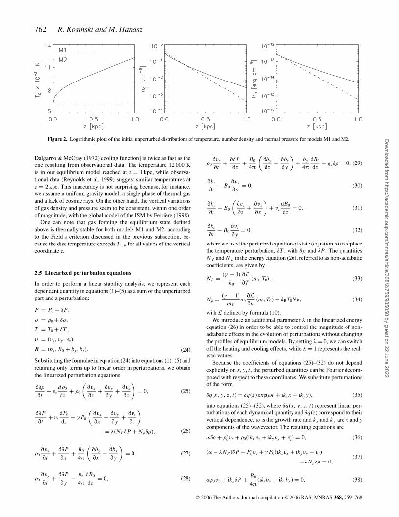
Figure 2. Logarithmic plots of the initial unperturbed distributions of temperature, number density and thermal pressure for models M1 and M2.

Dalgarno & McCray (1972) cooling function] is twice as fast as theone resulting from observational data. The temperature 12 000 Kis in our equilibrium model reached at z = 1 kpc, while observa-tional data (Reynolds et al. 1999) suggest similar temperatures atz = 2 kpc. This inaccuracy is not surprising because, for instance,we assume a uniform gravity model, a single phase of thermal gasand a lack of cosmic rays. On the other hand, the vertical variationsof gas density and pressure seem to be consistent, within one orderof magnitude, with the global model of the ISM by Ferriere (1998).

One can note that gas forming the equilibrium state definedabove is thermally stable for both models M1 and M2, accordingto the Field’s criterion discussed in the previous subsection, be-cause the disc temperature exceeds T crit for all values of the verticalcoordinate z.

2.5 Linearized perturbation equations

In order to perform a linear stability analysis, we represent eachdependent quantity in equations (1)–(5) as a sum of the unperturbedpart and a perturbation:

P = P0 + δP,

ρ = ρ0 + δρ,

T = T0 + δT ,

v = (vx , vy, vz),

B = (bx , B0 + by, bz). (24)

Substituting the formulae in equation (24) into equations (1)–(5) andretaining only terms up to linear order in perturbations, we obtainthe linearized perturbation equations

∂δρ

∂t+ vz

dρ0

dz+ ρ0

(∂vx

∂x+ ∂vy

∂y+ ∂vz

∂z

)= 0, (25)

∂δP∂t

+ vzdP0

dz+ γ P0

(∂vx

∂x+ ∂vy

∂y+ ∂vz

∂z

)= λ(NPδP + Nρδρ), (26)

ρ0∂vx

∂t+ ∂δP

∂x+ B0

4π

(∂by

∂x− ∂bx

∂y

)= 0, (27)

ρ0∂vy

∂t+ ∂δP

∂y− bz

4π

dB0

dz= 0, (28)

ρ0∂vz

∂t+ ∂δP

∂z+ B0

4π

(∂by

∂z− ∂bz

∂y

)+ by

4π

dB0

dz+ gzδρ = 0, (29)

∂bx

∂t− B0

∂vx

∂y= 0, (30)

∂by

∂t+ B0

(∂vz

∂z+ ∂vx

∂x

)+ vz

dB0

dz= 0, (31)

∂bz

∂t− B0

∂vz

∂y= 0, (32)

where we used the perturbed equation of state (equation 5) to replacethe temperature perturbation, δT , with δρ and δP . The quantitiesN P and N ρ in the energy equation (26), referred to as non-adiabaticcoefficients, are given by

NP = (γ − 1)

kB

∂L∂T

(n0, T0) , (33)

Nρ = (γ − 1)

mHn0

∂L∂n

(n0, T0) − kBT0 NP , (34)

with L defined by formula (10).We introduce an additional parameter λ in the linearized energy

equation (26) in order to be able to control the magnitude of non-adiabatic effects in the evolution of perturbations without changingthe profiles of equilibrium models. By setting λ = 0, we can switchoff the heating and cooling effects, while λ = 1 represents the real-istic values.

Because the coefficients of equations (25)–(32) do not dependexplicitly on x , y, t , the perturbed quantities can be Fourier decom-posed with respect to these coordinates. We substitute perturbationsof the form

δq(x, y, z, t) = δq(z) exp(ωt + ikx x + iky y), (35)

into equations (25)–(32), where δq(x , y, z, t) represent linear per-turbations of each dynamical quantity and δq(z) correspond to theirvertical dependence, ω is the growth rate and k x and k y are x and ycomponents of the wavevector. The resulting equations are

ωδρ + ρ ′0vz + ρ0(ikxvx + ikyvy + v′

z) = 0, (36)

(ω − λNP )δP + P ′0vz + γ P0(ikxvx + ikyvy + v′

z)

−λNρδρ = 0,(37)

ωρ0vx + ikxδP + B0

4π(ikx by − ikybx ) = 0, (38)


Dow


ic.oup.com/m



ωρ0vy + ikyδP − B ′0

4πbz = 0, (39)

ωρ0vz + δP ′ + B0

4π(b′

y − ikybz) + B ′0

4πby + gzδρ = 0, (40)

ωbx − iky B0vx = 0, (41)

ωby + B0(ikxvx + v′z) + B ′

0vz = 0, (42)

ωbz − iky B0vz = 0, (43)

where prime denotes the derivative with respect to the z coordinate.The above system of eight equations for eight unknown functions

of the z coordinate, δρ, δP , v x , v y , v z , bx , b y , bz , can be reduced toa single second-order differential equation for one unknown verticalvelocity component v z :

A1v′′z + A2v

′z + A3vz = 0. (44)

We describe the derivation of equation (44) from equations (36)–(43) in Appendix A. The coefficients A1, A2 and A3 depending onω, k x , k y and other parameters, as well as the coordinate z, aregiven in Appendix A. In the general case of z-dependent coefficients,equation (44) cannot be converted into an algebraic form. Therefore,the ordinary differential equation for the perturbation v z(z) shouldbe solved together with an appropriate set of boundary conditions.

2.6 Hot halo boundary conditions

In order to numerically solve the second-order ordinary differentialequation (44), one needs to specify two boundary conditions thatdeal with finite values of dynamical quantities on the vertical discboundaries.

A common disc equilibrium configuration considered in the liter-ature, in case of unstable astrophysical discs, is the disc–halo systemcomposed of two physically distinct components: the disc and hothalo. A physical justification for considering hot halos surroundingwarm discs follows from observations supported by theoretical mod-els. In real galaxies, the filling factor of hot gas grows up graduallywith height over the galactic mid-plane. In the present approach, wesimplify the configuration by assuming a sharp transition betweenthe warm disc and hot halo.

To follow this approach, we decompose the spatial domain intotwo regions: the disc in which solutions to equation (44) are con-structed with the aid of numerical integration, surrounded by semi-infinite upper and lower halo layers of different physical proper-ties, in which analytical solutions are available. By these means,boundary conditions for the disc extending in the range |z| � zb areimplied by a proper matching with external analytical solutions atthe disc–halo interface. Such an approach was originally applied byGoldreich & Lynden-Bell (1965) in studies of the gravitational in-stability of a rotating unmagnetized gaseous disc and then followedby Hanawa, Nakamura & Nakano (1992), Chou et al. (2000) andothers in studies of the Parker–Jeans instability of a magnetized,self-gravitating disc.

In forthcoming considerations, we implement the hot (adiabatic)halo solution of Hanawa et al. (1992) for the regions |z| � zb.

The general perturbations to the disc equilibrium can be decom-posed into symmetric and antisymmetric parts, referring to the gasdensity distribution with respect to the galactic mid-plane. However,for the uniform gravitational acceleration (utilized in our investiga-tion), which is discontinuous at z = 0, the unperturbed initial profile

possesses a cusp at z = 0, so the flow cannot move across the mid-plane. Thus, the only applicable solution in this case is the symmetricone. The boundary condition at the disc mid-plane (z = 0) is

vz(0) = 0. (45)

By considering the symmetric mode, we can restrict the physicaldomain to the upper half-space.

We assume that the hot halo extends above z > zb. To maintainvertical equilibrium, the total pressure must be continuous at thedisc–halo interface. We consider an asymptotic limit of the hot halowith temperature T h

0(z > zb) = ∞, density ρh0(z > zb) = 0 and

pressure Ph0(z > zb) = P 0(zb) = const, which fulfills equations (5)

and (14). We neglect cooling and heating in the hot halo (λ = 0) andseek solutions of equation (44) of the form

vz(x, y, z) = vhz (z) exp(ωt + ikx x + iky y), (46)

where

vhz (z) = V h

z exp(khz), (47)

kh is the spatial decay rate (in the z direction) of velocity pertur-bations in the halo and V h

z is a constant. From equation (44), weget

kh = ±√

k2x + k2

y . (48)

The requirement of vanishing perturbations at z = +∞ (Hanawaet al. 1992) implies that only the minus sign should be chosen in theupper halo, thus

vhz (z) = V h

z exp(−

√k2

x + k2y z

). (49)

Corresponding expressions for pressure and magnetic field pertur-bations in the halo region can be deduced with the aid of formulae(B1) and (B2) of Appendix B.

We note that the solution of equation (44), describing perturba-tions in the hot halo, differs formally from solutions of the sameequation in the disc (see Section 3.1), due to different propertiesof the unperturbed equilibrium in the disc and halo. One can notethat the amplitude of kinetic energy density perturbations is van-ishing for the halo linear solutions (due to vanishing gas density)and therefore it is bounded in the asymptotic limit of z → ∞, asrequired.

2.6.1 Matching conditions at the disc–halo interface

As we mentioned already, two boundary conditions are required tosolve equation (44). The analytical solutions corresponding to thehot halo make it possible to replace the boundary condition at z = ∞by a boundary condition at z = zb. The latter boundary condition canbe derived from the postulation of the continuity of the gas verticalvelocity component and the total (gas plus magnetic) pressure at thedisc–halo interface. These conditions can be formally expressed as

vz(zb + δz) = vhz (zb + δz), Ptot(zb + δz) = Ph

tot(zb + δz), (50)

where v z and Ptot denote the total pressure and velocity of the discgas and vh

z and Phtot denote the total pressure and velocity of the hot

halo gas. The original matching conditions are specified at z = zb

+ δz, because the contact surface between the disc and halo mediais subject to deformations by the gas motions.

We note that the temporal position of the contact surface atz = zb + δz is, in the linear regime, related to the vertical velocityperturbation by the relation

z = zb + vz(zb)/ω, (51)


Dow


ic.oup.com/m



where we utilized the fact that the linear vertical displacement δz isproportional to exp (ωt + i kxx + i kyy).

In order to implement the matching conditions in equation (50)in our considerations, we apply Taylor series expansion up to thelinear order and derive the corresponding conditions for linear per-turbations at z = zb. We obtain

vz(zb) = vhz (zb) (52)

for linear velocity perturbations and

P ′0(zb)δz + δP(zb) + B0(zb)B ′

0(zb)

4πδz + B0(zb)by(zb)

4π

= (Ph

0

)′(zb)δz + δPh(zb) + Bh

0 (zb)(

Bh0

)′(zb)

4πδz

+ Bh0 (zb)bh

y(zb)

4π

(53)

for the total pressure perturbations.The next step is to transform the latter condition (53) to the form

involving only the vertical velocity component and its derivativewith respect to the coordinate z. The final form of the matching con-dition for the vertical derivative of the vertical velocity componentis expressed in equation (B4) of Appendix B.

2.7 Numerical procedure and parameters

The full system of linearized MHD equations describing PI in thenon-adiabatic medium has been reduced to a single second-orderequation (44) that should be solved together with the boundary con-ditions: equation (45) at the mid-plane as well as equations (52) and(53) at the disc–halo interface.

Our present aim is to find the eigenvalues (the growth rate ω)and eigenstates of the system, i.e. such solutions of equation (44)that fulfill the set of boundary and matching conditions describedin previous subsections. Due to the complex z-dependence of thecoefficients A1, A2 and A3 of equation (44), we are going to constructnumerical solutions for the disc region and solve the resulting two-point boundary value problem with the aid of the shooting method(see e.g. Press et al. 1997). Refer to Appendix C for a detaileddescription of the method.

In the subsequent considerations, we examine the whole rangeof unstable azimuthal wavenumbers 0 � k y � 6 kpc−1 and fix theradial wavenumber to the plausible finite value k x = 10 kpc−1. Wecompared differences between cases k x = ∞ and k x = 10 kpc−1,finding that maximum growth rates are very similar in both casesand only a small change in ranges of azimuthal wavenumbers corre-sponding to unstable modes is noticeable. Therefore, the modes ofk x = 10 kpc−1 can be considered as representative for a wide rangeof radial wavenumbers.

We set the upper boundary at z = zb = 1 kpc. The remainingparameters, appearing in equation (44), are α, γ and λ. The valueof α = 1 is explained in Section 2.4. The choice of different valuesof γ makes it possible to investigate separately the adiabatic (γ =5/3) and isothermal (γ = 1) cases, when the non-adiabatic termsare switched off.

The parameter λ controls the magnitude of non-adiabatic ef-fects in the evolution of perturbations developing on top of the λ-independent equilibrium state: λ = 0 represents the adiabatic limit,and λ = 1 represents realistic rates of cooling and heating. We alsoconsider λ 1, in order to gain a better feeling of the influence ofnon-adiabatic effects on PI.

3 R E S U LT S

3.1 Classical case

First, we shall check if our perturbation equation (44) converges tothe classical dispersion relation after setting v z(z) = exp[ikzz +z/(2H )] and substituting expressions for A1, A2, A3 fromAppendix A. For a uniform temperature medium, in the absenceof heating and cooling (λ = 0) and in the limit k z = 0, we get

ω6 + ω4u20(2α + γ )

[k2

x + k2y

(4α + γ )

(2α + γ )+ 1

4H 2

]+ ω24u4

0α(α + γ )

{k4

y + k2x

[k2

y + (1 + α)(α + γ − 1)

4H 2α(α + γ )

]+ k2

y(1 + 2α)(γ − 1)

4H 2α(α + γ )

}+ 4k2

yu60α

2γ

{k4

y + k2x

[k2

y − (1 + α)(α − γ + 1)

2H 2αγ

]+ k2

y(2 + 3α)γ − 2(1 + α)2

4H 2αγ

}= 0, (54)

where u0 = √kB/mHT0 is the isothermal speed of sound and gz =

(1 + α)u20/H . This limiting case agrees with the result of Parker

(1967b). The dispersion relation (54) gives the maximum growthrates in the limit of infinite radial wavenumber k x .

We note finally that throughout the paper we plot and discussonly the lowest (fundamental) modes, i.e. the modes with the lowestnumber of nodes in the eigenstate, along the vertical direction, andthe largest growth rate among other modes. In the case of symmetricfundamental modes, there is only one node at z = 0 in the plot ofthe vertical component of velocity.

3.2 Model M1 (ΓUV)

We assume that the equilibrium temperature of model M1 does notdepend on z, and we consider eigenmodes of the system under thephotoionization heating (�UV) and the radiative cooling describedin previous sections.

In the following, we shall use the parameter λ for varying themagnitude of non-adiabatic effects in the evolution of perturbationswhile the unperturbed equilibrium remains fixed.

The equilibrium constructed in Section 2.4 can be applied forperturbations evolving with any value of λ.

In Fig. 3, we show the growth rate, ωR = Re(ω), versus theazimuthal wave number, k y , for γ = 5/3, α = 1, k x = 10 kpc−1

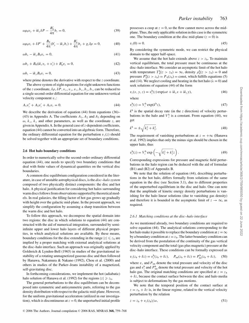
and zb = 1 kpc. Different curves are labelled with the magnitude ofthe parameter λ, which varies in the range [0, 102]. The adiabaticlimit is represented by λ = 0. We note that increasing the magnitudeof non-adiabatic effects (by rising the value of λ) results in greatergrowth rates and in larger ranges of unstable wavenumbers. The riseof the growth rate stops above λ = 1 (that curve appears slightlybelow the isothermal limit) and the curve for λ = 102 overlaps theisothermal limit (γ = 1).

The convergence of the non-adiabatic cases of model M1 to theisothermal limit can be understood because the presence of coolingand heating in the thermally stable system acts as an exchange ofthermal energy in-between different elements of gas.

Another issue is to understand why the isothermal limit admitshigher growth rates of PI than the adiabatic limit. The difference canbe explained by the fact that gas flow towards magnetic valleys isconvergent, therefore in the adiabatic limit it is subjected to heating


Dow


ic.oup.com/m



by the adiabatic compression. The rising temperature opposes thefurther compression and thereby the downflow of gas along mag-netic field lines is less efficient. Finally, the growth of the instabilityis limited. On the other hand, in the isothermal case where the com-pressed gas keeps the fixed temperature, the backreaction of thecompressed gas is weaker than in the adiabatic case. As it is appar-ent in Fig. 3, the rising magnitude of heating and cooling makes thesystem more and more similar to the isothermal case.

3.3 Model M2 (ΓUV+Γ1)

In this section, we incorporate the additional sources of heat postu-lated by Reynolds et al. (1999).

In Fig. 3, we display the growth rate ωR as a function of theazimuthal wavenumber k y for several different magnitudes of non-adiabatic effects λ. As before, the equilibrium configuration is com-mon for all presented cases for model M2. We note in Fig. 3 thesame tendency as in the case of model M1: the growth rate risesmonotonically as the magnitude of non-adiabatic effects rises up toλ = 1. The further growth of λ does not change the growth rate ofPI.

We note, however, differences between the adiabatic and isother-mal limits of models M2 and M1. The first difference appears inthe adiabatic limit. We find that model M2 is more stable in theadiabatic limit (λ = 0) than model M1. That difference can be at-tributed to different profiles of the equilibrium configuration. Thiscan be explained by referring to the stability criterion of the sys-tem of stratified gas and magnetic field (Lachieze-Rey et al. 1980),which for the adiabatic case can be written as

dT0

dz>

(γ − α − 1

1 + α

)T0

ρ0

dρ0

dz. (55)

In model M2, the vertical gradients of temperature are positive.Thus, this model tends to be more stable in the adiabatic limit thanmodel M1. For a sufficiently steep temperature profile, model M2can be completely stabilized in the adiabatic limit.

As it follows from Fig. 3, non-adiabatic processes intensify theinstability. The maximum growth rate is reached at the realisticcooling/heating rates (λ = 1).

Figure 3. Growth rates of PI in model M1 (left panel) and model M2 (right panel). The growth rate, computed with the assumption of hot halo boundaryconditions, is presented as a function of the wavenumber along the initial magnetic field direction. Each curve is labelled by the magnitude of non-adiabaticeffects λ (solid line). The curve labelled by λ = 0 represents the adiabatic case and γ = 1 represents the isothermal case (dashed line). The curve for λ = 102

coincides with the curve for γ = 1 in model M1 and with the curve for λ = 1 in model M2.

The basic difference between models M2 and M1 appears in theisothermal limit. As we noted already, the isothermal limit coincideswith the maximum growth rate reached for λ > 1 in model M1. Inmodel M2, the curve representing the non-adiabatic case (λ = 1)corresponds to a larger growth rate (by 20 per cent at maximum)and wider ranges of unstable wavenumbers than the ones obtainedfor the isothermal limit.

4 I N T E R P R E TAT I O N O F T H E R E S U LT S

We make the following test in order to find a reason for the addi-tional destabilization of model M2, above the isothermal limit, in thepresence of cooling and heating. We examine the three-dimensionalstructure of perturbations for selected dynamical quantities, accord-ing to formula (35), and find magnetic field lines by integration ofthe magnetic vector field.

In the presence of unstable Parker modes, magnetic field linesbecome undulatory. Their shape can be parametrized by the y coor-dinate. The vertical displacement amplitude z ≈ 0.5(zmax − zmin),determined for a single magnetic field line, grows proportionally toexp(ωt) and, in general, depends on the unperturbed position of thefield line z0. We compute temperature variations δT as a function ofposition along perturbed magnetic field lines. According to formula(24), the total temperature along magnetic field lines is, in the linearapproximation, given by

T [x(y), y, z(y), t] = T0[z(y)] + δT [x(y), y, z(y), t]. (56)

In Fig. 4, we show a plot of gas temperature along a single mag-netic field line for model M2. The line is chosen by varying itsstarting point in space, in order to find the line that is characterizedby the largest temperature variations along its length. We find that,for the vertical displacement amplitude of the order of 10 pc, thetotal temperature in magnetic valleys starts to decrease below thecritical value T crit, corresponding to the onset of TI. The loweredtemperature is associated with a lowered pressure in magnetic val-leys. The lowered pressure enables a faster downflow of gas towardsmagnetic valleys, a stronger buoyancy force acting on the tops ofmagnetic loops and thus a faster growth of PI.


Dow


ic.oup.com/m



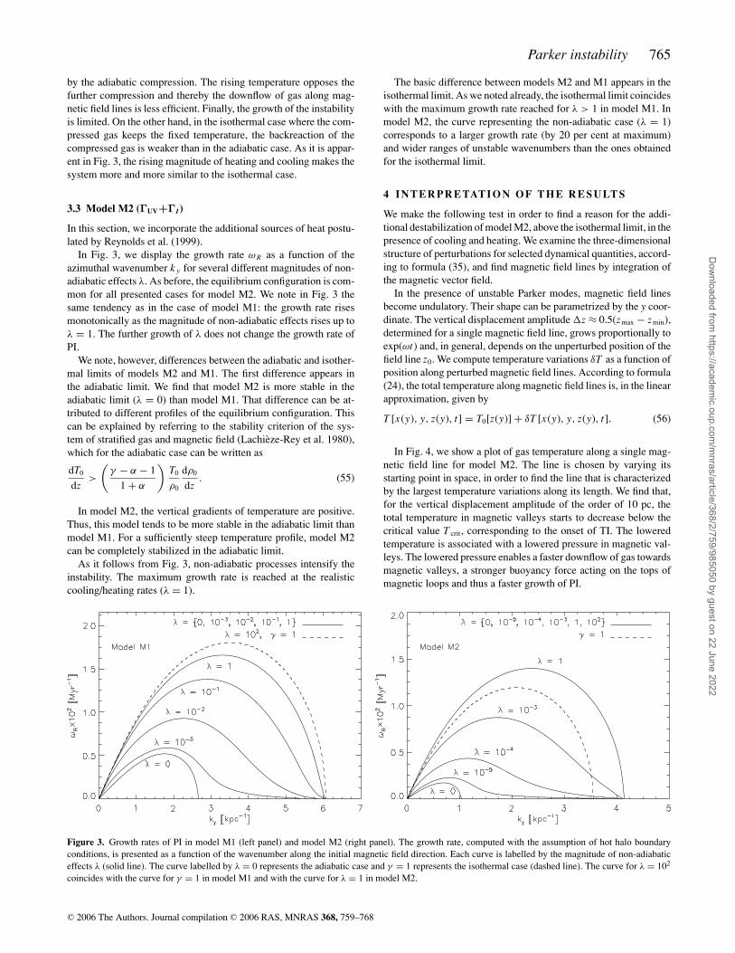
Figure 4. The distribution of gas temperature, along a magnetic field linefor the non-adiabatic case of model M2. The initially unperturbed magneticfield line placed at z = z0, with corresponding equilibrium gas tempera-ture T 0(z0), undulates due to the perturbation growth, so that temperaturebecomes lower in the magnetic valley and higher in the summit. The finaltemperature distribution (obtained through equation 56) along the perturbedfield line (solid line), gets steeper with respect to the unperturbed tempera-ture T 0(z) (obtained through equation 20) at the line position (dashed line).The displayed curves intersect at the point [z0, T 0(z0)].

Along with the declining temperature, a relatively small growthof density by factor 1.5 appears in the magnetic valleys of field linesdescribed above. The density variations due to PI itself, not includingthe possibility of the subsequent onset of TI, are consistent withprevious predictions by Kim et al. (1998). Therefore, TI followingPI in gas portions shifted below T crit is necessary to condense gassignificantly enough to form molecular clouds.

According to Fig. 4, the thermally stable gas above T min =T 0(0) = 6000 K can move in temperature space, due to linear PImodes, below T crit � 5840 K and thus may become thermally un-stable. Therefore, the development of PI modes may trigger TI assoon as the negative temperature perturbations reach a sufficientlylarge amplitude.

5 S U M M A RY A N D D I S C U S S I O N

In this paper, we have focused on the role of non-adiabatic effectson PI. We considered the radiative cooling approximated by theanalytic formula together with the heating effects of two kinds: (i)due to the background of UV stellar radiation (model M1); and (ii)supplemental sources of thermal energy (model M2) postulated byReynolds et al. (1999).

We performed a linear analysis of PI in the general three-dimensional case. In order to construct the unperturbed equilibria,we solved the magnetohydrostatic equilibrium equation along withthe thermal equilibrium equation. The latter equation appeared tosignificantly limit the space of available equilibrium states. We de-rived the second-order ordinary differential equation describing thevertical structure of eigenmodes of PI in the presence of cooling andheating. Subsequently, we showed that, in the limit of a vanishingmagnitude of non-adiabatic effects, equation (44) converges to theclassical dispersion relation derived by Parker (1967b). We numer-ically solved the two-point boundary value problem, consisting ofequation (44) and the hot halo boundary conditions.

Next, we examined the effects of two types of heat sources. Inthe case of model M1 (pure photoionization heating), the maximum

growth rate of the instability and the range of unstable modes growsmonotonically until the magnitude of non-adiabatic effects reachesrealistic values. Further increasing the magnitude of non-adiabaticeffects does not change the maximum growth rate. In model M1 (nosupplemental heat sources), the growth rate of PI in the presence ofnon-adiabatic effects appears to be comparable, although slightlylower than the isothermal limit. In model M2 (including supple-mental heat sources), the maximum growth rate of PI is larger thanthe one corresponding to the isothermal limit. The enlargement ofthe maximum growth rates, due to non-adiabatic effects, above theisothermal limit is rather minor (∼20 per cent).

We note that the previous study by Ames (1973) has shown onlya moderate enlargement of the growth rate above the adiabatic limit.The comparison of models M1 and M2 leads to the conclusion thatthe most essential modification of the properties of PI is due to sup-plemental heat sources, postulated by Reynolds et al. (1999), i.e.those terms that make the heating function different from photoion-ization heating.

We note that we were able to investigate the modifications causedby non-adiabatic effects only within each of the models M1 andM2. The comparison of maximum growth rates between these twomodels makes no sense because the underlying equilibrium config-urations are different. On the other hand, finding a common equi-librium for all models was not possible because the different heat-ing functions of models M1 and M2 impose different equilibriumtemperature profiles. Therefore, the adiabatic and isothermal limits,within each model, appear to be good reference solutions for thenon-adiabatic cases.

On the other hand, the non-adiabatic evolution of the density per-turbations of model M2 closely follows the isothermal evolution ofmodel M1, i.e. the magnitude of density perturbations is not sig-nificantly enhanced in the non-adiabatic case of model M2. Thislast statement would suggest that non-adiabatic effects do not im-prove conditions for the formation of molecular clouds by PI itself;however, at the same time, the temperature decreases in magneticvalleys, contrary to the adiabatic and isothermal cases.

This qualitatively new behaviour of the system may have impor-tant consequences for the subsequent evolution of the ISM, whichundergoes realistic heating and cooling processes. By realistic heat-ing, we mean photoionization heating by the UV radiation and thesupplemental heat sources postulated by Reynolds et al. (1999); byrealistic cooling, we mean the one represented by the Dalgarno &McCray (1972) cooling function. In those conditions, the tempera-ture decreasing mechanism implied by PI may shift large portionsof gas below the temperature T crit, which is slightly lower than theassumed minimum equilibrium gas temperature 6000 K. Therefore,the development of PI modes may trigger TI in magnetic valleys assoon as the temperature drops locally below T crit.

The above scenario differs from the one discussed by Ames(1973). The difference follows from the fact that the equilibriumconfiguration considered by Ames is thermally unstable, thus short-wavelength thermal modes are present among the unstable eigen-modes of the system. These modes enhance the formation of gasclumps, as a combined action of PIs and TIs only if the equi-librium configuration is thermally unstable. In our model, how-ever, the thermal gas occupying the temperature range 6000 K <

T < 12 000 K, representing the warm ionized medium, is thermallystable.

We predict therefore, on the basis of linear analysis of PI, that,in the presence of realistic cooling and heating, PI may transferthermally stable ionized gas to the thermally unstable regime. Inthis way, PI may trigger the formation of molecular clouds.


Dow


ic.oup.com/m



Although the growth rate of PI in the presence of non-adiabaticeffects is not drastically accelerated by non-adiabatic effects, wepoint out that the decrement of gas temperature in magnetic valleysand the possible subsequent onset of TI form a qualitatively newsituation as far as the formation of molecular clouds by means of PIis concerned.

Recently, Lee et al. (2004) and Lee & Hong (2005) stressed theimportance of self-gravity as a driving agent for PI. They performlinear stability analysis and two-dimensional numerical MHD sim-ulations of Parker–Jeans instability and suggest that the cooperationof the both instabilities can overcome major difficulties of PI con-sidered as a driver of GMCs.

We admit that the effects of self-gravity apparently help to over-come some of difficulties. However, we are inclined to formulate ahypothesis that the presence of non-adiabatic effects, leading finallyto the onset of TI, is essential for the formation of GMCs by PI. Therole of TI is to remove the excess of thermal energy: the major agentacting against condensation of clouds.

AC K N OW L E D G M E N T S

This work was supported by the Polish Committee for Scientific Re-search (KBN) through the grant PB 0656/P03/2004/26. We thankBoud Roukema for language corrections of the manuscript and ac-knowledge an anonymous referee for constructive comments.

R E F E R E N C E S

Ames S., 1973, ApJ, 182, 387Blitz L., Shu F. H., 1980, ApJ, 238, 148Chou W., Matsumoto R., Tajima T., Umekawa M., Shibata K., 2000, ApJ,

538, 710

Dalgarno A., McCray R. A., 1972, ARA&A, 10, 375Domgorgen H., Mathis J. S., 1994, ApJ, 428, 647Ferriere K., 1998, ApJ, 497, 759Field G. B., 1965, ApJ, 142, 531Foglizzo T., Tagger M., 1994, A&A, 287, 297Franco J., Kim J., Alfaro E. J., Hong S. S., 2002, ApJ, 570, 647Giz A. T., Shu F. H., 1993, ApJ, 404, 185Goldreich P., Lynden-Bell D., 1965, MNRAS, 130, 97Goncalves D. R., Jatenco-Pereira V., Opher R., 1993, ApJ, 414, 57Haffner L. M., Reynolds R. J., Tufte S. L., 1999, ApJ, 523, 223Hanasz M., Lesch H., 2000, ApJ, 543, 235Hanasz M., Lesch H., 2003, A&A, 412, 331Hanasz M., Otmianowska-Mazur K., Lesch H., 2002, A&A, 386, 347Hanawa T., Nakamura F., Nakano T., 1992, PASJ, 44, 509Kim J., Ryu D., 2001, ApJ, 561, L135Kim J., Hong S. S., Ryu D., 1997, ApJ, 485, 228Kim J., Hong S. S., Ryu D., Jones T. W., 1998, ApJ, 506, L139Kuwabara T., Nakamura K., Ko C. M., 2004, ApJ, 607, 828Lachieze-Rey M., Asseo E., Cesarsky C. J., Pellat R., 1980, ApJ, 238, 175Lee S. M., Hong S. S. 2005, astro-ph/0503013Lee S. M., Kim J., Franco J., Hong S. S., 2004, J. Korean Astron. Soc. 37,

249Mouschovias T. Ch., Shu F. H., Woodward P. R., 1974, A&A, 33, 73Parker E. N., 1953a, ApJ, 117, 169Parker E. N., 1953b, ApJ, 117, 431Parker E. N., 1966, ApJ, 145, 811Parker E. N., 1967a, ApJ, 149, 517Parker E. N., 1967b, ApJ, 149, 535Parker E. N., Jokipii J. R., 2000, ApJ, 536, 331Press W. H., Flannery B. P., Teukolsky S. A., Vetterling W. T., 1997, Nu-

merical recipes. Cambridge Univ. Press, CambridgeReynolds R. J., Haffner L. M., Tufte S. L., 1999, ApJ, 525, L21Santillan A., Kim J., Franco J., Martos M. A., Hong S. S., Ryu D., 2000,

ApJ, 545, 353Shu F. H., 1974, A&A, 33, 55Skibo J. G., Ramaty R., Purcell W. R., 1996, A&AS, 120, 403

A P P E N D I X A : T H E D E R I VAT I O N O F E QUAT I O N (44)

By algebraic transformations, we convert the set of linearized Fourier decomposed first-order differential equations (36)–(43) for eightunknown z functions, δρ, δP , v x , v y , v z , bx , b y , bz , into one second-order differential equation (44) for v z . With the equilibrium equations(13)–(16) in mind, the construction is as follows.

First, with the aid of equation (36), we replace δρ in equation (37) and get the equation for δP:

δP = I1(ikxvx + ikyvy + v′z) + I2vz . (A1)

Using equations (36), (41), (42), (43) and (A1) and differentiated equations (42) and (A1) with respect to z, variables δρ, bx , b y , bz and δPcan be eliminated in equations (38), (39) and (40) to give respectively

J1vx = kx ky I1vy − ikx (J2vz + J3v′z), (A2)

J4vy = kx ky I1vx − iky(J2vz + I1v′z), (A3)

J5vz + J6v′z + J3v

′′z = −ikx (J7vx + J3v

′x ) + iky(J8vy − I1v

′y). (A4)

We eliminate v y in equation (A2) using equation (A3):

vx = ikx (K1vz + K2v′z). (A5)

The same manipulation can be made to eliminate v x in equation (A3) through equation (A2):

vy = iky(K3vz + K4v′z). (A6)

The last operation is aimed to eliminate v x and v y along with their derivatives from equation (A4) by means of equations (A5) and (A6). Theresult is equation (44) with coefficients A1, A2 and A3 of the form

A1 = J3 − k2x J3 K2 − k2

y I1 K4,


Dow


ic.oup.com/m



A2 = J6 − k2x [J7 K2 + J3(K1 + K ′

2)] − k2y[I1(K3 + K ′

4) − J8 K4],

A3 = J5 − k2x (J7 K1 + J3 K ′

1) + k2y(J8 K3 − I1 K ′

3).(A7)

The coefficients I 1, I 2, J 1, J 2, J 3, J 4, J 5, J 6, J 7, J 8, K 1, K 2, K 3, K 4 are given by

I0 = ω(ω − λNP ),

I1 = −(λNρ + ωγ u2

0

)ρ0/I0,

I2 = −[(1 + α)λNρρ′0 − ωgzρ0]/[(1 + α)I0], (A8)

J1 = ωρ0 − k2x I1 + 2α

ω

(k2

x + k2y

)u2

0ρ0, J2 = gzα

(1 + α)ωρ0 + I2, J3 = I1 − 2α

ωu2

0ρ0,

J4 = ωρ0 − k2y I1, J5 = ωρ0 + 2α

ωk2

yu20ρ0 − gz

(1 + α)ωρ ′

0 + I ′2,

J6 = (2α − 1)gz

(1 + α)ωρ0 + I2 + I ′

1, J7 = (α − 1)gz

(1 + α)ωρ0 + I ′

1, J8 = gz

ωρ0 − I ′

1,(A9)

K0 = k2x k2

y I 21 − J1 J4, K1 = J2

(k2

y I1 + J4

)/K0, K2 = (

k2y I 2

1 + J3 J4

)/K0,

K3 = J2

(k2

x I1 + J1

)/K0, K4 = I1

(k2

x J3 + J1

)/K0.

(A10)

Prime denotes the z derivative, and u0 = √kB/mHT0 is the z-dependent speed of sound.

A P P E N D I X B : T H E D I S C – H A L O M AT C H I N G C O N D I T I O N

The matching condition for the z derivative of the vertical velocity component can be derived as follows.Quantities δP , δPh, b y , bh

y in equation (53) are to be expressed by velocities v z , vhz and their derivatives v′

z , (vhz )′. From equations (39), (43)

and (A6), we get

δP = (L1 − L2 K3)vz − L2 K4v′z . (B1)

Similarly, the equation for b y results from equations (42) and (A5):

by = 1

ω

(B0k2

x K1 − B ′0

)vz − B0

ω

(1 − k2

x K2

)v′

z . (B2)

We define coefficients K1 to K4 in Appendix A, and

L1 = − αgz

(1 + α)ωρ0, L2 = ωρ0. (B3)

After the substitution of equations (B1) and (B2) into the total pressure continuity condition (53), we obtain[B2

0

(K2k2

x − 1)

4πω− K4 L2

]v′

z(zb) +[(

Bh0

)2(K h

2 k2x −1

)4πω

− K h4 Lh

2

](vh

z

)′(zb) +

[B2

0 K1−(

Bh0

)2K h

1

]k2

x

4πωvh

z (zb)

+[

P ′0−

(Ph

0

)′

ω+ L1 − Lh

1 − K3 L2 + K h3 Lh

2

]vh

z (zb) = 0. (B4)

All quantities in these equations are evaluated in z = zb.

A P P E N D I X C : T H E S H O OT I N G M E T H O D

We compute iteratively the unknown growth rate ω, appearing explicitly in equation (44), for fixed values of k x and k y . We start with a guessedvalue ω = ωg, which may be equal to the growth rate corresponding to the isothermal case or to any other value. It should be noted, however,that not every choice of the ωg leads to a successful solution.

Next, we numerically integrate equation (44) from the upper disc boundary at z = zb towards the galactic mid-plane at z = 0 using thefourth-order Runge–Kutta method with a variable step. The starting values of v z(zb) and its vertical derivative v′

z(zb) are deduced from theanalytical halo solutions (49) (for which the constants V h

z and V hz can be chosen arbitrarily, because we deal with the linear problem) with

the aid of matching conditions (52) and (53). The latter condition is further replaced by equation (B4) in Appendix B, expressing the pressurematching in terms of v z(zb) and v′

z(zb).The boundary condition (45) at z = 0 is not fulfilled for an arbitrary initial guess ωg. The resulting value vz,ωg (0) obtained from the numerical

integration is in general different to the values of v z(0) required by the boundary condition at z = 0. In a series of iterations, we slightly correctωg by taking ωg + ωg and repeat the integration until F(ωg) = 0 is true to the required accuracy, where F(ωg) = vz,ωg (0) for symmetricmodes. In case of a convergent iteration, the limit of a series of ωg is considered as the eigenvalue ω. An efficient way of finding roots ofthe non-linear equation F(ω) = 0 is based on a numerical root-finder utilizing the secant method. In this way, we numerically find the lineargrowth rate, ω, as a function of radial k x and azimuthal k y components of the wavevector.

This paper has been typeset from a TEX/LATEX file prepared by the author.


Dow


ic.oup.com/m


On the influence of cooling and heating processes on Parker ...

Documents