On the Existence of Non-Supersymmetric Black Hole Attractors for Two-Parameter Calabi-Yau's and Attractor Equations

arX

iv:h

ep-t

h/06

0713

2v3

17

Sep

2006

hep-th/0607132

On the Existence of Non-Supersymmetric Black Hole Attractors forTwo-Parameter Calabi-Yau’s and Attractor Equations

Payal Kaura(a)1 and Aalok Misra(a),(b)2

(a) Indian Institute of Technology Roorkee, Roorkee - 247 667, Uttaranchal, India(b) Enrico Fermi Institute, University of Chicago, Chicago, IL 60637, USA

Abstract

We look for possible nonsupersymmetric black hole attractor solutions for type II compactification on(the mirror of) CY3(2, 128) expressed as a degree-12 hypersurface in WCP4[1, 1, 2, 2, 6]. In the process,(a) for points away from the conifold locus, we show that the existence of a non-supersymmetric attractoralong with a consistent choice of fluxes and extremum values of the complex structure moduli, couldbe connected to the existence of an elliptic curve fibered over C8 which may also be “arithmetic” (insome cases, it is possible to interpret the extremization conditions for the black-hole superpotential asan endomorphism involving complex multiplication of an arithmetic elliptic curve), and (b) for pointsnear the conifold locus, we show that existence of non-supersymmetric black-hole attractors corresponds

to a version of A1-singularity in the space Image(Z6 → R2

Z2(→ R3)) fibered over the complex structure

moduli space. The (derivatives of the) effective black hole potential can be thought of as a real (integer)projection in a suitable coordinate patch of the Veronese map: CP5 → CP20, fibered over the complexstructure moduli space. We also discuss application of Kallosh’s attractor equations (which are equivalentto the extremization of the effective black-hole potential) for nonsupersymmetric attractors and show that(a) for points away from the conifold locus, the attractor equations demand that the attractor solutionsbe independent of one of the two complex structure moduli, and (b) for points near the conifold locus,the attractor equations imply switching off of one of the six components of the fluxes. Both these featuresare more obvious using the atractor equations than the extremization of the black hole potential.

1email: [email protected]: [email protected]

1

1 Introduction

It has been shown that extremal black holes exhibit an interesting phenomenon - attractor mechanism [1]-the moduli are “attracted” to some fixed values determined by the charges of the black hole, independentof the asymptotic values of the moduli. Supersymmetric black holes at the attractor point, correspond tominimizing the central charge and the effective black hole potential, whereas nonsupersymmetric attractors[2], which have recently been (re)discussed [3], at the attractor point, correspond to minimizing only thepotential and not the central charge. Recently, attractor equations for (non) supersymmetric black holesand flux vacua were given by Kallosh [4] (For an earlier derivation, see [5]3), and some examples verifyingthe same were studied in [7] including IIB compactified on one-parameter Calabi-Yau’s - the attractorequations, however, are equivalent to extremizing the effective black hole potential (See [6] and referencestherein). In this paper, we discuss the existence of possible nonsupersymmetric attractor solutions to typeIIB compactified on a two-parameter Calabi-Yau, both, from the equivalent points of view of extremizing aneffective black-hole potential and also by using the attractor equations. We get some interesting connectionsbetween arithmetic and geometry and nonsupersymmetric black-hole attractors. We emphasize that westress more on the forms of the various equations rather than their numerical content.

The plan of the paper is as follows. Section 2 consists of the bulk of the calculations and results asregards the non-supersymmetric black hole attractors from minimizing the effective black-hole potential. Itis divided into two parts - 2.1 deals with points in the moduli space away from the singular conifold locus,and 2.2 deals with points near the same - 2.1 is further subdivided into two parts: 2.1.1 deals with positiveeigenvalues of the mass matrix and 2.1.2 deals with null eigenvalues of the mass matrix. Section 3 has adiscussion on the use of the new attractor equations of [4] to get non-supersymmetric attractors; it is dividedinto two (short) parts - 3.1 is for points in the moduli space away from the singular conifold locus and 3.2is for points close to the same. There are three appendices relevant to the calculations in sections 2 and 3.Section 4 has the conclusions and discussion on future directions.

2 The Black Hole Potential Extremization, the Mass Matrix and At-tractor Solutions

In this section we work out possible attractor solutions obtained by extremizing the effective black-holepotential for points in the moduli space, both away and near the conifold locus of the mirror to a two-parameter Calabi-Yau with h1,1 = 2, h2,1 = 128, expressed as a degree-12 hypersurface in WCP4[1, 1, 2, 2, 6].

2.1 Away from the Singular Conifold Locus

The defining hypersurface for the mirror to the aforementioned Calabi-Yau is:

x20 + x12

1 + x122 + x6

3 + x64 − 12ψx0x1x2x3x4 − 2φx6

1x62 = 0, (1)

with h1,1 = 128 and h2,1 = 2. Under the symplectic decomposition of the holomorphic three-form Ω canonicalhomology (Aa, B

a, a = 1, 2, 3) and cohomology bases (αa, βa), defining the periods as

∫

AaΩ = za,

∫

Ba Ω = Fa,

3We thank S.Ferrara for bringing [5] to our attention

2

such that Ω = zaαa−Faβa. Then, the Kahler potential K is given by: −ln(−i(τ − τ)− ln(−i

∫

CY Ω∧ Ω) =

ln(−i(τ − τ)) − ln(−iΠ†ΣΠ), Π being the six-component period vector and Σ =

(

0 13

−13 0

)

.

Expanding about a point in the moduli space away from the conifold locus, such as φ = 2 (or equivalentlyz = 0) and ψ = 0 (See [8, 9, 10]), one gets the following period vector:

Π = −i18 (−1 + (−1)

112 )π

72 (−576 2F1(

112 ,

712 , 1,

14) + 48 z 2F1(

112 ,

712 , 1,

14) + 7 z 2F1(

1312 ,

1912 , 2,

14 ))

213 Γ(5

6)3 ,

−i72

π (2

23 (3 + 2 i+ 4 (−1)

112 + (−1)

712 )π

52 (−576 2F1(

112 ,

712 , 1,

14 ) + 48 z 2F1(

112 ,

712 , 1,

14) + 7 z 2F1(

1312 ,

1912 , 2,

14))

Γ(56)

3

−108ψ2 (−128√

6EllipticK(2

3) + 32

√6 z EllipticK(

2

3) + 9π z 2F1(

5

4,7

4, 2,

1

4))),

( 118 − i

18 )π72 (−576 2F1(

112 ,

712 , 1,

14) + 48 z 2F1(

112 ,

712 , 1,

14) + 7 z 2F1(

1312 ,

1912 , 2,

14 ))

213 Γ(5

6 )3 ,

−i36

π (2

23 π

52 (−576 2F1(

112 ,

712 , 1,

14) + 48 z 2F1(

112 ,

712 , 1,

14 ) + 7 z 2F1(

1312 ,

1912 , 2,

14))

Γ(56)

3 −54ψ2 (−128√

6EllipticK(2

3)

+32√

6 z EllipticK(2

3) + 9π z 2F1(

5

4,7

4, 2,

1

4))),

i

72π (

223 π

52 (−576 2F1(

112 ,

712 , 1,

14 ) + 48 z 2F1(

112 ,

712 , 1,

14 ) + 7 z 2F1(

1312 ,

1912 , 2,

14))

Γ(56 )

3 −54ψ2 (−128√

6EllipticK(2

3)

+32√

6 z EllipticK(2

3) + 9π z 2F1(

5

4,7

4, 2,

1

4))),

−i72

π (2

23 (1 + (−1)

712 )π

52 (−576 2F1(

112 ,

712 , 1,

14) + 48 z 2F1(

112 ,

712 , 1,

14 ) + 7 z 2F1(

1312 ,

1912 , 2,

14))

Γ(56 )

3

−108ψ2 (−128√

6EllipticK(2

3) + 32

√6 z EllipticK(

2

3) + 9π z 2F1(

5

4,7

4, 2,

1

4))),

where the complete elliptic integral of the first kind EllipticK(ν) ≡∫

π2

0dφ√

1−νsin2φ. One then constructs the

superpotential:

W = fTΠ =1

72π (

−2 i 223 (−1 + (−1)

112 ) f1 π

52 (−576 2F1(

112 ,

712 , 1,

14) + 48 z 2F1(

112 ,

712 , 1,

14) + 7 z 2F1(

1312 ,

1912 , 2,

14 ))

Γ(56 )

3

+(2 − 2 i) 2

23 f3 π

52 (−576 2F1(

112 ,

712 , 1,

14 ) + 48 z 2F1(

112 ,

712 , 1,

14 ) + 7 z 2F1(

1312 ,

1912 , 2,

14))

Γ(56)

3

−i F6 (2

23 (1 + (−1)

712 )π

52 (−576 2F1(

112 ,

712 , 1,

14) + 48 z 2F1(

112 ,

712 , 1,

14 ) + 7 z 2F1(

1312 ,

1912 , 2,

14))

Γ(56 )

3

3

−108ψ2 (−128√

6EllipticK(2

3) + 32

√6 z EllipticK(

2

3) + 9π z 2F1(

5

4,7

4, 2,

1

4)))

−i f1 (2

23 (3 + 2 i+ 4 (−1)

112 + (−1)

712 )π

52 (−576 2F1(

112 ,

712 , 1,

14) + 48 z 2F1(

112 ,

712 , 1,

14) + 7 z 2F1(

1312 ,

1912 , 2,

14))

Γ(56 )

3

−108ψ2 (−128√

6EllipticK(2

3) + 32

√6 z EllipticK(

2

3) + 9π z 2F1(

5

4,7

4, 2,

1

4)))

−2 i f4 (2

23 π

52 (−576 2F1(

112 ,

712 , 1,

14) + 48 z 2F1(

112 ,

712 , 1,

14 ) + 7 z 2F1(

1312 ,

1912 , 2,

14))

Γ(56 )

3

−54ψ2 (−128√

6EllipticK(2

3) + 32

√6 z EllipticK(

2

3) + 9π z 2F1(

5

4,7

4, 2,

1

4)))

+i F5 (2

23 π

52 (−576 2F1(

112 ,

712 , 1,

14) + 48 z 2F1(

112 ,

712 , 1,

14 ) + 7 z 2F1(

1312 ,

1912 , 2,

14))

Γ(56 )

3

−54ψ2 (−128√

6EllipticK(2

3) + 32

√6 z EllipticK(

2

3) + 9π z 2F1(

5

4,7

4, 2,

1

4))))

The Kahler potential is given by:

K = − log

(

a+b ψ2+c z+dψ2 z+g z ψ2+b ψ2+c z+h z z+j ψ2 z z+ψ2 g z+d ψ2 z+z j ψ2 z+i k ψ2 ψ2 (−z+z))

,

from which one calculates the metric:

gij =

(

gzz gzψgψz gψψ

)

, (2)

where

gzz =c2 − ah+ h2 z z

(a+ c z + c z)2,

gψψ =4 |ψ|2 (g z + b+ d z) (b+ d z + g z)

(a+ c z + c z)2,

gzψ =2 ψ ((c+ h z) (g z + b+ d z) − (a+ c z + c z) (g + j z))

(a+ c z + c z)2.

The effective black hole potential in type II theories is given by:

V = eK(gijDiWDjW + |W |2), (3)

W being the superpotential, K the Kahler potential and the covariant derivative DiW ≡ ∂iW + ∂iKW .The first derivative of the potential is given by (See [11]):

∂iV = eK(gjkDiDjWDkW + ∂igjkDjWDkW + 2DiWW ). (4)

4

Using the results of the appendix A, one can see that for |z| << 1, |ψ| << 1, up to O(terms second orderin z and/or ψ and their complex conjugates) in the numerators and the denominators,

gijDzDiWDjW , ∂zgijDiWDjW ∼

∑

l

eiαlarg(y)

(

al + blz + clz

a′l + b′lz + c′lz

)

,

DzWW ∼ a+ bz + cz

a′ + b′z + c′z, (5)

and

gijDψDiWDjW , ∂zgijDiWDjW ∼ 1

|ψ|∑

l

eiαlarg(ψ)

(

al + blz + clz

a′l + b′lz + c′lz

)

,

DψWW ∼ ψ

(

a+ bz + cz

a′ + b′z + c′z

)

. (6)

where αi = 2,−2, 0. This implies that

∂zV ∼∑

i

eiαiarg(ψ)(

Ai +Biz + Ciz

A′i +B′

iz + C ′iz

)

,

∂ψV ∼ 1

|ψ|∑

i

eiαiarg(ψ)(

Ai +Biz + Ciz

A′i +B′

iz + C ′iz

)

. (7)

If one complexifies and projectivizes the fis, then the effective potential extremization conditions ∂zV =∂ψV = 0 could correspond to real integer projections of intersection of quadrics in a suitable patch ofCP5(f1 : ... : f6) fibered over C(z)×R(arg(y)), which correspond to four real non-linear constraints on thesix flux components fis and the two complex complex structure moduli z, ψ. It is interesting to note thatthe expression ∂iV , for a given extremum values of the complex structure moduli (for complex projective

space valued fis) would correspond to the Veronese map: CP5(f1 : ... : f6) → CP20(f21 : f1f2 : ... : f2

6 )(∼ C6

Z2

where the Z2 flips the signs of all the fis). Veronese surfaces and maps have been shown to have connectionwith moduli spaces relevant to MSSM (See [12]).

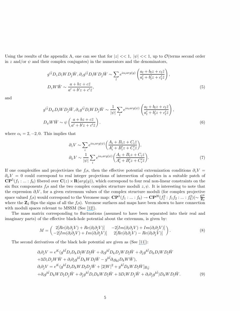
The mass matrix corresponding to fluctuations (assumed to have been separated into their real andimaginary parts) of the effective black-hole potential about the extremum, is given by:

M =

(

2[Re(∂i∂jV ) +Re(∂i∂jV )] −2[Im(∂i∂jV ) + Im(∂i∂jV )]−2[Im(∂i∂jV ) + Im(∂i∂jV )] 2[Re(∂i∂jV ) −Re(∂i∂jV )]

)

. (8)

The second derivatives of the black hole potential are given as (See [11]):

∂i∂jV = eK(gklDiDkDlWDlW + ∂igklDkDjWDlW + ∂jg

klDkDiWDlW

+3DiDjWW + ∂i∂jgklDkWDlW − gkl∂igklDkWW ),

∂i∂jV = eK(gklDiDkWDlDjW + [2|W |2 + gklDkWDlW ]gij

+∂igklDkWDlDjW + ∂jg

klDiDkWDlW + 3DiWDjW + ∂i∂jgkl)DkWDlW . (9)

5

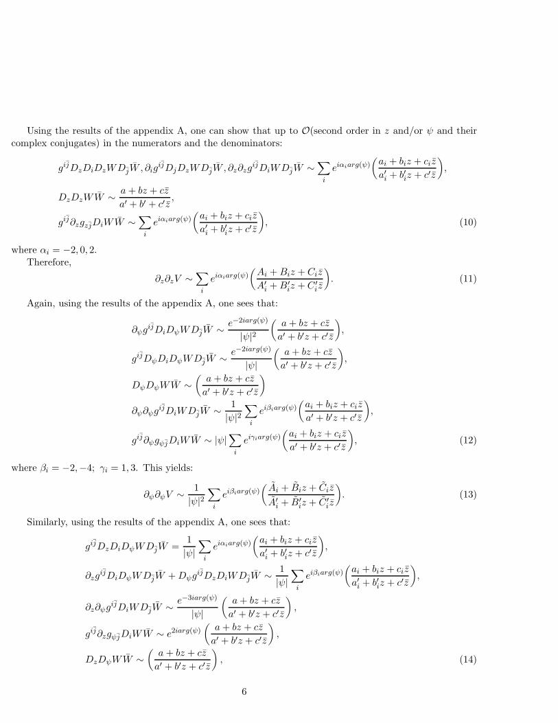
Using the results of the appendix A, one can show that up to O(second order in z and/or ψ and theircomplex conjugates) in the numerators and the denominators:

gijDzDiDzWDjW , ∂igijDjDzWDjW , ∂z∂zg

ijDiWDjW ∼∑

i

eiαiarg(ψ)(

ai + biz + ciz

a′i + b′iz + c′z

)

,

DzDzWW ∼ a+ bz + cz

a′ + b′ + c′z,

gij∂zgzjDiWW ∼∑

i

eiαiarg(ψ)(

ai + biz + ciz

a′i + b′iz + c′z

)

, (10)

where αi = −2, 0, 2.Therefore,

∂z∂zV ∼∑

i

eiαiarg(ψ)(

Ai +Biz + Ciz

A′i +B′

iz +C ′iz

)

. (11)

Again, using the results of the appendix A, one sees that:

∂ψgijDiDψWDjW ∼ e−2iarg(ψ)

|ψ|2(

a+ bz + cz

a′ + b′z + c′z

)

,

gijDψDiDψWDjW ∼ e−2iarg(ψ)

|ψ|

(

a+ bz + cz

a′ + b′z + c′z

)

,

DψDψWW ∼(

a+ bz + cz

a′ + b′z + c′z

)

∂ψ∂ψgijDiWDjW ∼ 1

|ψ|2∑

i

eiβiarg(ψ)(

ai + biz + ciz

a′ + b′z + c′z

)

,

gij∂ψgψjDiWW ∼ |ψ|∑

i

eiγiarg(ψ)(

ai + biz + ciz

a′ + b′z + c′z

)

, (12)

where βi = −2,−4; γi = 1, 3. This yields:

∂ψ∂ψV ∼ 1

|ψ|2∑

i

eiβiarg(ψ)(

Ai + Biz + Ciz

A′i + B′

iz + C ′iz

)

. (13)

Similarly, using the results of the appendix A, one sees that:

gijDzDiDψWDjW =1

|ψ|∑

i

eiαiarg(ψ)(

ai + biz + ciz

a′i + b′iz + c′z

)

,

∂zgijDiDψWDjW +Dψg

ijDzDiWDjW ∼ 1

|ψ|∑

i

eiβiarg(ψ)(

ai + biz + ciz

a′i + b′iz + c′z

)

,

∂z∂ψgijDiWDjW ∼ e−3iarg(ψ)

|ψ|

(

a+ bz + cz

a′ + b′z + c′z

)

,

gij∂zgψjDiWW ∼ e2iarg(ψ)(

a+ bz + cz

a′ + b′z + c′z

)

,

DzDψWW ∼(

a+ bz + cz

a′ + b′z + c′z

)

, (14)

6

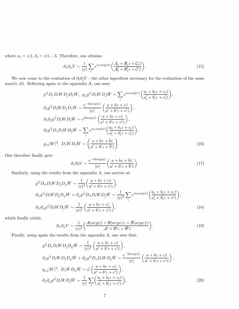
where αi = ±1, βi = ±1,−3. Therefore, one obtains:

∂z∂ψV ∼ 1

|ψ|∑

i

eiγiarg(ψ)(Ai + Biz + CizA′i + B′

iz + C′z

)

. (15)

We now come to the evaluation of ∂i∂jV - the other ingredient necessary for the evaluation of the massmatrix (8). Referring again to the appendix A, one sees:

gijDzDiWDjDzW , gijgijDiWDJW ∼

∑

i

eiαiarg(ψ)(

ai + biz + ciz

a′i + b′iz + c′iz

)

,

∂zgijDiWDjDzW ∼ e−3iarg(ψ)

|ψ|

(

a+ bz + cz

a′ + b′z + c′z

)

,

∂z∂zgijDiWDjW ∼ e2iarg(ψ)

(

a+ bz + cz

a′ + b′z + c′z

)

,

∂zgijDzDiWDjW ∼

∑

i

eiαiarg(ψ)(

ai + biz + ciz

a′i + b′iz + c′iz

)

,

gzz|W |2, DzWDzW ∼(

a+ bz + bz

a′ + b′z + b′z

)

. (16)

One therefore finally gets:

∂z∂zV ∼ e−3iarg(ψ)

|ψ|

(

a+ bz + bz

a′ + b′z + b′z

)

. (17)

Similarly, using the results from the appendix A, one arrives at:

gijDψDiWDjDψW ∼ 1

|ψ|2(

a+ bz + cz

a′ + b′z + c′z

)

,

∂ψgijDiWDjDψW + ∂ψg

ijDψDiWDjW ∼ 1

|ψ|2∑

i

eiαiarg(ψ)(

ai + biz + ciz

a′i + b′iz + c′z

)

,

∂ψ∂ψgijDiWDjW ∼ 1

|ψ|2(

a+ bz + cz

a′ + b′z + c′z

)

, (18)

which finally yields:

∂ψ∂ψV ∼ 1

|ψ|2(A(argψ) + B(argψ)z + B(argψ)z

A′ + B′z + B′z

)

. (19)

Finally, using again the results from the appendix A, one sees that:

gijDzDiWDjDψW ∼ 1

|ψ|2(

a+ bz + cz

a′ + b′z + c′z

)

,

∂zgijDiWDjDψW + ∂ψg

ijDzDiWDjW ∼ e−2iarg(ψ)

|ψ|

(

a+ bz + cz

a′ + b′z + c′z

)

,

gzψ|W |2, DzWDψW ∼ ψ

(

a+ bz + cz

a′ + b′z + c′z

)

,

∂z∂ψgijDiWDjW ∼ 1

|ψ|∑

i

(

ai + biz + ciz

a′i + b′iz + c′z

)

, (20)

7

which gives:

∂z∂ψV ∼ 1

|ψ|2(

a+ bz + cz

a′ + b′z + c′z

)

. (21)

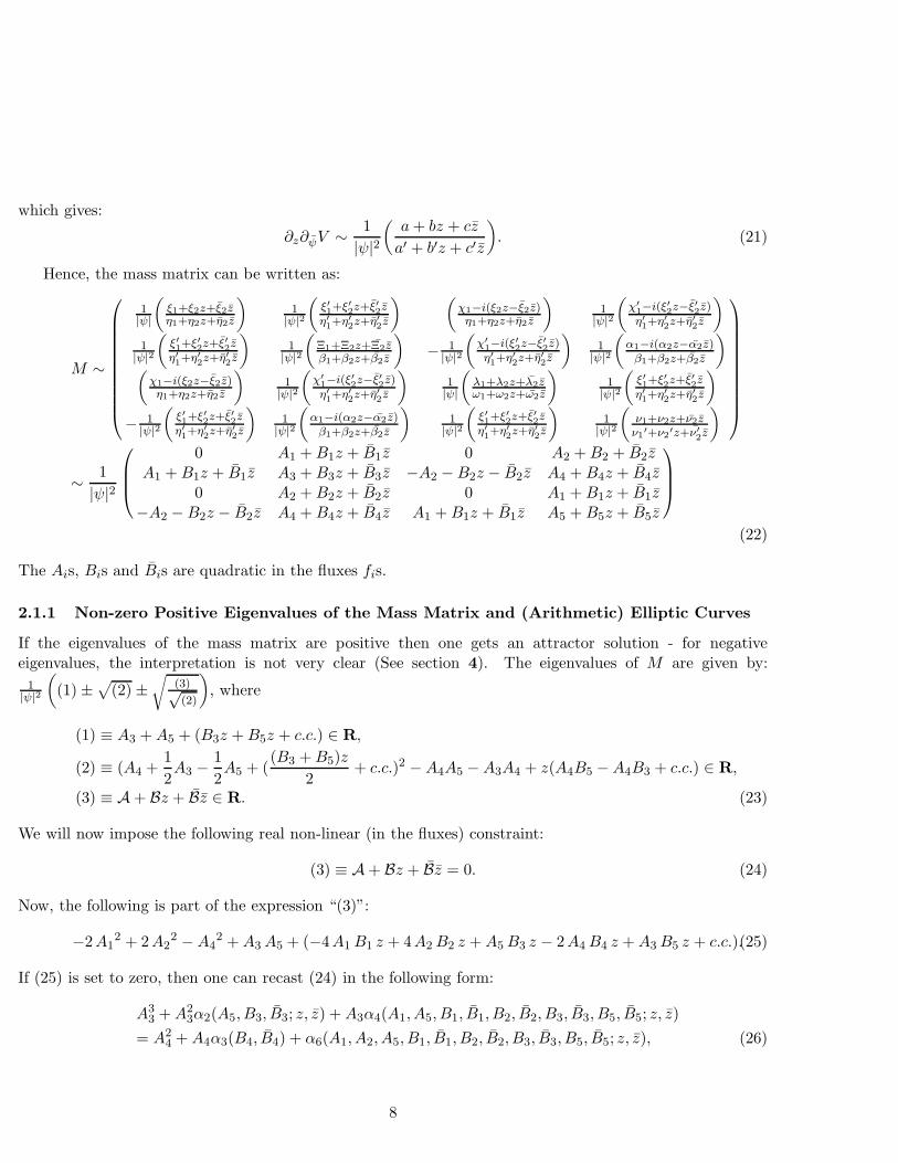
Hence, the mass matrix can be written as:

M ∼

1|ψ|

(

ξ1+ξ2z+ξ2zη1+η2z+η2z

)

1|ψ|2

(

ξ′1+ξ′2z+ξ′

2z

η′1+η′2z+η′

2z

) (

χ1−i(ξ2z−ξ2z)η1+η2z+η2z

)

1|ψ|2

(

χ′

1−i(ξ′

2z−ξ′

2z)η′1+η′2z+η

′

2z

)

1|ψ|2

(

ξ′1+ξ′2z+ξ′

2z

η′1+η′2z+η′

2z

)

1|ψ|2

(

Ξ1+Ξ2z+Ξ2zβ1+β2z+β2z

)

− 1|ψ|2

(

χ′

1−i(ξ′

2z−ξ′

2z)η′1+η′2z+η

′

2z

)

1|ψ|2

(

α1−i(α2z−α2z)β1+β2z+β2z

)

(

χ1−i(ξ2z−ξ2z)η1+η2z+η2z

)

1|ψ|2

(

χ′

1−i(ξ′

2z−ξ′

2z)η′1+η′2z+η

′

2z

)

1|ψ|

(

λ1+λ2z+λ2zω1+ω2z+ω2z

)

1|ψ|2

(

ξ′1+ξ′

2z+ξ′

2z

η′1+η′2z+η′

2z

)

− 1|ψ|2

(

ξ′1+ξ′2z+ξ′

2z

η′1+η′2z+η′

2z

)

1|ψ|2

(

α1−i(α2z−α2z)β1+β2z+β2z

)

1|ψ|2

(

ξ′1+ξ′2z+ξ′

2z

η′1+η′2z+η′

2z

)

1|ψ|2

(

ν1+ν2z+ν2zν1′+ν2′z+ν′2z

)

∼ 1

|ψ|2

0 A1 +B1z + B1z 0 A2 +B2 + B2zA1 +B1z + B1z A3 +B3z + B3z −A2 −B2z − B2z A4 +B4z + B4z

0 A2 +B2z + B2z 0 A1 +B1z + B1z−A2 −B2z − B2z A4 +B4z + B4z A1 +B1z + B1z A5 +B5z + B5z

(22)

The Ais, Bis and Bis are quadratic in the fluxes fis.

2.1.1 Non-zero Positive Eigenvalues of the Mass Matrix and (Arithmetic) Elliptic Curves

If the eigenvalues of the mass matrix are positive then one gets an attractor solution - for negativeeigenvalues, the interpretation is not very clear (See section 4). The eigenvalues of M are given by:

1|ψ|2

(

(1) ±√

(2) ±√

(3)√(2)

)

, where

(1) ≡ A3 +A5 + (B3z +B5z + c.c.) ∈ R,

(2) ≡ (A4 +1

2A3 −

1

2A5 + (

(B3 +B5)z

2+ c.c.)2 −A4A5 −A3A4 + z(A4B5 −A4B3 + c.c.) ∈ R,

(3) ≡ A + Bz + Bz ∈ R. (23)

We will now impose the following real non-linear (in the fluxes) constraint:

(3) ≡ A + Bz + Bz = 0. (24)

Now, the following is part of the expression “(3)”:

−2A12 + 2A2

2 −A42 +A3A5 + (−4A1 B1 z + 4A2B2 z +A5B3 z − 2A4B4 z +A3B5 z + c.c.).(25)

If (25) is set to zero, then one can recast (24) in the following form:

A33 +A2

3α2(A5, B3, B3; z, z) +A3α4(A1, A5, B1, B1, B2, B2, B3, B3, B5, B5; z, z)

= A24 +A4α3(B4, B4) + α6(A1, A2, A5, B1, B1, B2, B2, B3, B3, B5, B5; z, z), (26)

8

which, is an elliptic curve fibered over C8(A1 + iarg(y), A2 + iA5, B1, B2, B3, B4, B5, z). One can compare(26) with the following elliptic curve over any field:

y2 + a1xy + a3y = x3 + a2x2 + a4x+ a6, (27)

for which the j-invariant is defined as: j =(a21+4a2)2−24(a1a3+a4)

∆ where the discriminant ∆ ≡ −(a21 +

4a2)2(a2

1a6−a1a3a4 +a2a23 +4a2a6−a2

4)+9(a21 +4a2)(a1a3 +2a4)(a

23 +4a6)−8(a1a3 +2a4)

3−27(a23 +4a6)

2.Interestingly, the equations (7) can be rewritten as:

(

A1 −C1B1zC2

A2 −C1B2zC2

)

(

1−C2

C1

)

= −C1z

(

1−C2

C1

)

. (28)

If the 2 × 2 matrix in (28) is SL(2,Z)-valued, then (28) can be compared with following endomorphismE → E requiring λ(Z + τZ) ⊂ Z + τZ, λ ∈ C, for an elliptic curve E = C/(Z + τZ):

(

N A−C M

)

= λ

(

1τ

)

, (29)

implying a complex multiplication Z+ωZ represented as: m11+m2

( 12(d+ b) a

−c 12(D − b)

)

, where (A,N −M,C) = l(a, b, c) (l being the greater common factor) and D ≡ b2 − 4ac (See [14]). The modular parameterτ , which is supposed to satisfy: aτ2 + bτ + c = 0, gets identified with −C2

C1. It would be interesting to see if

one could further impose the condition that this value of τ satisfies the above definition of the j-invariantfunction where it is understood that j = j(τ = −C2

C1, Ai, Bi, Bi). Such an elliptic curve is what is

referred to as an “arithmetic elliptic curve” (See [14])4.To ensure that the eigenvalues are real, we now impose the following additional real and again non-

linear(in the fluxes) constraint:

−A4A5 −A3A4 + z(A4B5 −A4B3 + c.c.) = 0. (30)

Thus one is guaranteed to have two, doubly degenerate, real eigenvalues of M , 1|ψ|2

((1) ±√

2). One thus

sees the possibility of getting attractor as well as repeller (see section 4) solutions dependingon whether (1) >

√2 or (1) <

√2.

To summarize, from (7), one gets two complex, or four real constraints and then three additional realconstraints from (24), (30) and (25) on the six integer-valued fluxes fis, the complex structure moduli z, ψ.

4Related to complex multiplication, one can choose a Weierstrass model for E given by(See [15]):

y2 = 4x3 − c(x+ 1), c =

27j

j − (12)3, j 6= 0, (12)3,

y2 = x

3 = 1, j = 0,

y2 = x

3 + x, j = (12)3.

If gcd(a, b, c) = 1 and D is the fundamnetal discriminant (which means a discriminant of a quadratic imaginary field KD ≡Q[i√

|D|] = a + ib√

|D| : a, b ∈ Q), then j(τ ) is an algebraic integer of order equal to the number of equivalence classes of

integral binary forms

(

a b2

b2

c

)

using SL(2,Z)-valued matrices for similarity transformations. Also, KD(j(τi) is Galois over

KD and independent of τi, where each τi corresponds to the distinct ideal classes in the order O(KD).

9

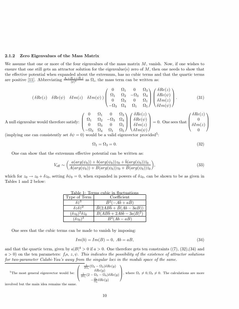
2.1.2 Zero Eigenvalues of the Mass Matrix

We assume that one or more of the four eigenvalues of the mass matrix M , vanish. Now, if one wishes toensure that one still gets an attractor solution for the eigenvalue(s) zero of M , then one needs to show thatthe effective potential when expanded about the extremum, has no cubic terms and that the quartic termsare positive [11]. Abbreviating Ai+Biz+Biz

|ψ|2 as Ωi, the mass term can be written as:

( δRe(z) δRe(ψ) δIm(z) δIm(ψ) )

0 Ω1 0 Ω3

Ω1 Ω2 −Ω3 Ω4

0 Ω3 0 Ω1

−Ω3 Ω4 Ω1 Ω5

δRe(z)δRe(ψ)δIm(z)δIm(ψ)

. (31)

A null eigenvalue would therefore satisfy:

0 Ω1 0 Ω3

Ω1 Ω2 −Ω3 Ω4

0 Ω3 0 Ω1

−Ω3 Ω4 Ω1 Ω5

δRe(z)δRe(ψ)δIm(z)δIm(ψ)

= 0. One sees that

δRe(z)0

δIm(z)0

(implying one can consistently set δψ = 0) would be a valid eigenvector provided5:

Ω1 = Ω3 = 0. (32)

One can show that the extremum effective potential can be written as:

Veff ∼(

a(arg(ψ0)) + b(arg(ψ0))z0 + b(arg(ψ0))z0A(arg(ψ0)) +B(arg(ψ0))z0 + B(arg(ψ0))z0

)

, (33)

which for z0 → z0 + δz0, setting δψ0 = 0, when expanded in powers of δz0, can be shown to be as given inTables 1 and 2 below:

Table 1: Terms cubic in fluctuationsType of Term Coefficient

δz3 B2(−Ab+ aB)

δzδz2 B(2ABb+ B(Ab− 3aB))

(δz0)2δz0 B(ABb+ 2Abb− 3a|B|2)

(δz0)3 B2(Ab− aB)

One sees that the cubic terms can be made to vanish by imposing:

Im(b) = Im(B) = 0, Ab = aB, (34)

and that the quartic term, given by a|B|4 > 0 if a > 0. One therefore gets ten constraints ((7), (32),(34) anda > 0) on the ten parameters: fis, z, ψ. This indicates the possibility of the existence of attractor solutionsfor two-parameter Calabi-Yau’s away from the singular loci in the moduli space of the same.

5The most general eigenvector would be:

12Ω1

(Ω4 − Ω2)δRe(y)δRe(y)

12Ω1

(2 − Ω3 − Ω4)δRe(y)

−Ω1Ω3δRe(y)

, where Ω1 6= 0,Ω3 6= 0. The calculations are more

involved but the main idea remains the same.

10

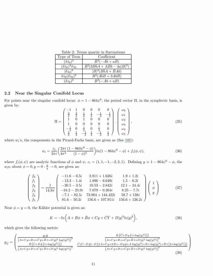
Table 2: Terms quartic in fluctuationsType of Term Coefficient

(δz0)4 B3(−Ab+ aB)

(δz0)3δz0 B2(3BbA+ABb− 4a|B|2)

|δz0|4 |B|2(BbA+ BAb)

δz0(δz0)3 B2(AbB + 3AbB)

(δz0)4 B3(−Ab+ aB)

2.2 Near the Singular Conifold Locus

For points near the singular conifold locus: φ = 1 − 864ψ6, the period vector Π, in the symplectic basis, isgiven by:

Π =

−1 1 0 0 0 032

32

12

12 −1

2 −12

1 0 1 0 0 01 0 0 0 0 0−1

2 0 12 0 1

2 012

12 −1

212 −1

212

.

ω0

ω1

ω2

ω3

ω4

ω5

, (35)

where wi’s, the components in the Picard-Fuchs basis, are given as (See [10]):

wi =ci

2πi

(

2πi

4π2

(1 − 864ψ6 − φ)

(1 − φ)2

)

ln(1 − 864ψ6 − φ) + fi(φ,ψ), (36)

where fi(φ,ψ) are analytic functions of φ and ψ, ci = (1, 1,−1,−2, 2, 1). Defining y ≡ 1 − 864ψ6 − φ, thewis, about φ = 0, y = 0 : φ

y→ 0, are given as:

f0

f1

f2

f3

f4

f5

=1

14.8π

−11.6 − 0.5i 2.811 + 1.626i 1.9 + 1.2i−13.3 − 1.4i 1.896 − 6.649i 1.5 − 6.2i−20.5 − 3.5i 10.53 − 2.842i 12.1 − 24.4i−34.2 − 25.9i 7.079 − 0.264i 8.25 − 7.7i−7.1 − 82.5i 73.904 + 144.422i 58.7 + 138i81.6 − 50.2i 156.6 + 107.911i 156.6 + 126.2i

1φy

(37)

Near φ = y = 0, the Kahler potential is given as:

K = −ln(

A+Bφ+ Bφ+ Cy + CY +D|y|2ln|y|2)

, (38)

which gives the following metric:

gij =

B B

(A+C y+B z+C y+B z+D |y|2 log(|y|2))2

B (C+D y (1+log(|y|2)))(A+C y+B z+C y+B z+D |y|2 log(|y|2))

2

B (C+D y (1+log(|y|2)))(A+C y+B z+C y+B z+D |y|2 log(|y|2))

2

C (C−D y)−D (2A+C y+2B z−Dy y+A log(|y|2)+B z log(|y|2)+B z (2+log(|y|2)))(A+C y+B z+C y+B z+D |y|2 log(|y|2))

2

(39)

11

Using the results of the appendices B and C, one can see that for |φ| << 1, |y| << 1,

gijDφDiWDjW , ∂φgijDiWDjW ,

∼ |ln(y)|2ln(|y|2)

(

a+ bφ+ cφ+ fy + gy + hy ln(y) + ky ln(y) + lyln(y) +myln(y) + n|y|2ln(|y|2)a′ + b′φ+ c′φ+ f ′y + g′y + n′|y|2ln(|y|2)

)

,

DφWW ∼(

a+ bφ+ cφ+ fy + gy + hy ln(y) + ky ln(y) + lyln(y) +myln(y) + n|y|2ln(|y|2)a′ + b′φ+ c′φ+ f ′y + g′y + n′|y|2ln(|y|2)

)

(40)

and

gijDyDiWDjW , ∂φgijDiWDjW ,DφWW

∼(

ln(y)

yln(|y|2) ,|ln(y)|2y(ln|y|2)2 , ln(y)

)

(

a+ bφ+ cφ+ fy + gy + hy ln(y) + ky ln(y) + lyln(y) +myln(y) + n|y|2ln(|y|2)a′ + b′φ+ c′φ+ f ′y + g′y + n′|y|2ln(|y|2)

)

.

(41)

In equations (40), (41) and other similar equations below, it is assumed that only the forms and not thedetails of the different terms, apart from the (ln|y|)α pieces, are the same. This implies that

∂φV ∼ ln|y|(

a+ bφ+ cφ+ fy + gy + hy ln(y) + ky ln(y) + lyln(y) +myln(y) + n|y|2ln(|y|2)a′ + b′φ+ c′φ+ f ′y + g′y + n′|y|2ln(|y|2)

)

,

∂ψV ∼ 1

|y|

(

a+ bφ+ cφ+ fy + gy + hy ln(y) + ky ln(y) + lyln(y) +myln(y) + n|y|2ln(|y|2)a′ + b′φ+ c′φ+ f ′y + g′y + n′|y|2ln(|y|2)

)

. (42)

For the purpose of constructing the mass matrix, one needs to evaluate second derivatives of the blackhole potential.

Using the results of the appendices B and C, one can show that up to O(second order terms in z and/ory and their complex conjugates) in the numerators and denominators:

gijDφDiDφWDjW , ∂igijDjDφWDjW , ∂φ∂φg

ijDiWDjW ,DφDφWW, gij∂φgφjDiWW

∼(

1 orln|y|ln|y|2 ,

ln|y|ln|y|2 , 1,

ln|y|ln|y|2

)

(

a+ bφ+ cφ+ fy + gy + hy ln(y) + ky ln(y) + lyln(y) +myln(y) + n|y|2ln(|y|2)a′ + b′φ+ c′φ+ f ′y + g′y + n′|y|2ln(|y|2)

)

.

(43)

Therefore,

∂φ∂φV ∼(

a+ bφ+ cφ+ fy + gy + hy ln(y) + ky ln(y) + lyln(y) +myln(y) + n|y|2ln(|y|2)a′ + b′φ+ c′φ+ f ′y + g′y + n′|y|2ln(|y|2)

)

. (44)

Again, using the results of the appendices B and C, one sees that:

∂ygijDiDyWDjW , DyDyWW, gij∂ygyjDiWW, gijDyDiDyWDjW , ∂ψ∂ψg

ijDiWDjW

∼( |ln(y)|2y(ln|y|2)2 ,

1

y,

1

|y| ,1

y2ln(y),

|ln(y)|2y2(ln|y|2)2 ,

)

×(

a+ bφ+ cφ+ fy + gy + hy ln(y) + ky ln(y) + lyln(y) +myln(y) + n|y|2ln(|y|2)a′ + b′φ+ c′φ+ f ′y + g′y + n′|y|2ln(|y|2)

)

. (45)

12

This yields:

∂y∂yV ∼ 1

|y|2(ln|y|)2

(

a+ bφ+ cφ+ fy + gy + hy ln(y) + ky ln(y) + lyln(y) +myln(y) + n|y|2ln(|y|2)a′ + b′φ+ c′φ+ f ′y + g′y + n′|y|2ln(|y|2)

)

.

(46)Similarly, using the results of the appendix B, one sees that:

gijDφDiDyWDjW , ∂zgijDiDψWDjW +Dψg

ijDzDiWDjW , ∂z∂ψgijDiWDjW , gij∂zgψjDiWW, DzDψWW

∼(

ln(y

y ln|y|2 ,1

|y| , ln(y),|ln(y)|2y(ln|y|2)2 , ln(y)

)

×(

a+ bφ+ cφ+ fy + gy + hy ln(y) + ky ln(y) + lyln(y) +myln(y) + n|y|2ln(|y|2)a′ + b′φ+ c′φ+ f ′y + g′y + n′|y|2ln(|y|2)

)

. (47)

Therefore, one obtains:

∂φ∂yV ∼ 1

|y|

(

a+ bφ+ cφ+ fy + gy + hy ln(y) + ky ln(y) + lyln(y) +myln(y) + n|y|2ln(|y|2)a′ + b′φ+ c′φ+ f ′y + g′y + n′|y|2ln(|y|2)

)

. (48)

We now come to the evaluation of ∂i∂jV - the other ingredient necessary for the evaluation of the massmatrix (8). Referring again to the appendix B, one sees:

gijDφDiWDjDφW , gijgijDiWDJW , ∂φg

ijDiWDjDφW , ∂φ∂φgijDiWDjW , ∂φg

ijDφDiWDjW , |W |2gφφ, DφWDφW

∼(

ln|y|, ln|y|, ln|y|, 1, ln|y|, 1, 1)

(

a+ bφ+ cφ+ fy + gy + hy ln(y) + ky ln(y) + lyln(y) +myln(y) + n|y|2ln(|y|2)a′ + b′φ+ c′φ+ f ′y + g′y + n′|y|2ln(|y|2)

)

.

(49)

One therefore finally gets:

∂φ∂φV ∼ ln|y|(

a+ bφ+ cφ+ fy + gy + hy ln(y) + ky ln(y) + lyln(y) +myln(y) + n|y|2ln(|y|2)a′ + b′φ+ c′φ+ f ′y + g′y + n′|y|2ln(|y|2)

)

. (50)

Similarly, using the results from the appendix B, one arrives at:

gijDyDiWDjDyW , ∂ygijDiWDjDyW + ∂yg

ijDyDiWDjW , ∂y∂ygijDiWDjW , DyWDyW , |W |2gyy

∼(

1

|y|2(ln|y|)2 ,1

|y|2ln|y| ,1

|y|2ln|y| , |ln(y)|2, ln|y|2)

×(

a+ bφ+ cφ+ fy + gy + hy ln(y) + ky ln(y) + lyln(y) +myln(y) + n|y|2ln(|y|2)a′ + b′φ+ c′φ+ f ′y + g′y + n′|y|2ln(|y|2)

)

(51)

which finally yields:

∂y∂yV ∼ 1

|y|2ln|y|

(

a+ bφ+ cφ+ fy + gy + hy ln(y) + ky ln(y) + lyln(y) +myln(y) + n|y|2ln(|y|2)a′ + b′φ+ c′φ+ f ′y + g′y + n′|y|2ln(|y|2)

)

.

(52)

13

Finally, using again the results from the appendices B and C, one sees that:

gijDzDiWDjDyW , ∂φgijDiWDjDyW + ∂yg

ijDφDiWDjW , ∂φ∂ygijDiWDjW , |W |2gφy, DφWDyW

∼(

ln(y)

yln|y|2 ,ln(y)

|y| ,1

|y| , ln|y|2, ln(y)

)

×(

a+ bφ+ cφ+ fy + gy + hy ln(y) + ky ln(y) + lyln(y) +myln(y) + n|y|2ln(|y|2)a′ + b′φ+ c′φ+ f ′y + g′y + n′|y|2ln(|y|2)

)

, (53)

which gives:

∂φ∂yV ∼ ln|y||y|

(

a+ bφ+ cφ+ fy + gy + hy ln(y) + ky ln(y) + lyln(y) +myln(y) + n|y|2ln(|y|2)a′ + b′φ+ c′φ+ f ′y + g′y + n′|y|2ln(|y|2)

)

. (54)

One thus sees that the mass matrix of (8) is given by (retaining again only the most dominant terms):

M ∼ 1

|y|2

0 0 0 00 Λ1 0 Λ2

0 0 0 00 Λ2 0 Λ3

, (55)

where Λi ≡(

ai+biφ+biφ+fiy+fiy+hiy ln(y)+hiy ln(y)+liyln(y)+liyln(y)+ni|y|2ln(|y|2)

a′i+b′

iφ+b′

iφ+f ′

iy+f ′

iy+n′

i|y|2ln(|y|2)

)

. Hence, M will have at least

one doubly degenerate null eigenvalue. One corresponding eigenvector of fluctuations in φ and y will be

given by:

δRe(φ)0

δIm(φ)0

, alongwith the constraint:

Λ22 = Λ1Λ3. (56)

Thus, from equations (34), (42), (56) and “a > 0”, one gets nine constraints on the six fluxes fis and thecomplex structure moduli φ, y.

One has to remember that the Λis are real-valued quantities constructed from the square of the fluxes andthe complex structure moduli at the extremum of the effective black-hole potential. This is very interesting- Λi ∈ R, which implies that one gets, for null eigenvalues of the mass matrix, for points in the moduli spacenear the singular conifold locus, a version of an A1-singularity wherein one gets the embedding: R

2

Z2→ R3,

which is the real projection of the familiar T ∗(S2) for C2

Z2→ C3 - in short, the singular conifold locus in the

moduli space of the two-parameter Calabi-Yau, corresponds to some version of A1-singularity in the spaceImage(Z6 → R

2

Z2(→ R3)) fibered over C2(φ, y), when looking for nonsupersymmetric black-hole attractor

solutions.

3 Attractor equations for non-supersymmetric Attractors

In this section, we now discuss getting non-supersymmetric attractor solutions using the “new attractor”equations of Kallosh [4], which are as follows:

Σ.f = 2eKIm

(

W Π − gijDiWDjΠ

)

. (57)

14

3.1 Away from the conifold locus

Using the results of appendix A, one can show that the RHS, up to terms linear in the complex structuremoduli, z, ψ is independent of ψ, and the attractor equations can be written as:

f4

f5

f6

−f1

−f2

−f3

=

a1+b1z+c1za′1+b′1z+c

′

1za2+b2z+c2za′2+b′2z+c

′

2za3+b3z+c3za′3+b′3z+c

′

3za4+b4z+c4za′4+b′4z+c

′

4za5+b5z+c5za′5+b′5z+c

′

5za6+b6z+c6za′6+b′6z+c

′

6z

, (58)

where ai, bi, ci depend on the fluxes fis. This is not in contradiction with the analysis of section 2, where itis shown that the results depend, at best, on the phase of ψ and not its modulus - the attractor equations goone step further in showing that the attractors are also independent of the phase. The attractor equations(58) bring out a feature, which would become apparent in the analysis of section 2 involving extremizationof the effective black-hole potential only after a complete numerical calculation, namely that for points awayfrom the conifold locus, the nonsupersymmetric attractors are independent of one of the complex structuremoduli (ψ).

3.2 Near the conifold locus

Using results of appendices B and C, one sees that

Im(W Π) ∼

Σ1

Σ2

Σ3

Σ4

Σ5

Σ6

and

Im(gijDiWDjΠ ∼ gyyDyWDyΠ) ∼ |ln(y)|2ln|y|2

000Σ4

00

,

where

Σ4, Σi ≡(

ai + biφ+ biφ+ fiy + fiy + hiy ln(y) + hiy ln(y) + liyln(y) + liyln(y) + ni|y|2ln(|y|2)a′i + b′iφ+ b′iφ+ f ′iy + f ′i y + n′i|y|2ln(|y|2)

)

.

The only way to satisfy the attractor equations (57) is to impose

f1 = Σ4 = 0. (59)

15

Thus, the attractor equations show that the attractor solutions of section 2 (obtained by extremization ofthe effective black hole potential and analysis of the eigenvalues of the mass matrix) must include switchingoff of one of the six components of the fluxes - this would become apparent only after a complete numericalanalysis of section 2.

4 Conclusion

We looked at an example of (the mirror to) a two-parameter Calabi-Yau (expressed as a hypersurface in aweighted complex projective space) and looked at possible non-supersymmetric black-hole attractor solutionsby extremization of an effective potential, for points away and close to the singular conifold locus. For theformer, we showed a connection between non-supersymmetric black hole attractors and an elliptic curve andfound a system of seven (for positive eigenvalues of the mass matrix for points in the moduli space awayfrom the conifold locus) or nine (for null eigenvalues of the mass matrix for points in the moduli space nearthe conifold locus) or ten (for null eigenvalues of the mass matrix for points in the moduli space away fromthe conifold locus) constraints on the six integer fluxes and the two complex structure moduli. It might bepossible to interpret the black-hole extremization as an endomorphism involving complex multiplication ofa possibly arithmetic elliptic curve. For points close to the conifold locus, we found a connection betweennon-supersymmetric black hole attractors and an A1 singularity. From the point of view of the attractorequations of [4], we saw that for the former case, the nonsupersymmetric attractor solutions are independentof one of the two complex structure moduli. For the latter, the attractor equations of [4] imply switchingoff of one of the six components of the fluxes. Both would become manifest only after a detailed numericalcomputation involving extremization of the effective potential and analysis of mass matrix eigenvalues andtherefore serve as good checks on the numerics involved in the analysis of section 2 - one must howevermake note of the fact that the black hole potential extremization analysis, even without doing any detailednumerical analysis, already tells us that the nonsupersymmetric attractors for points in the moduli spaceaway from the singular conifold locus, can have, at best, only a phase-factor dependence on ψ and areindependent of |ψ|, and the attractor equations analysis says that even the phase factor dependence isabsent. The mass matrix can take negative eigenvalues, in addition to positive and null - the eigenmodesfor the negative eigenvalues could perhaps be interpreted as non-supersymmetric repellers6, or might beinterpretable as a flop transition in the extended Kahler cone [13].

Using tools from computational algebraic geometry, one could hope to do a better job in actually doingthe numerical computations related to the present work on supersymmetric black-hole attractors (and also

6This was suggested by R.Kallosh to one of us(AM).

16

flux vacua ([16]) attractors) 7. Attractor basins ([7]) and area codes, is another aspect which could belooked into. Further, it would be nice to see whether the particular Calabi-Yau considered in this work isan “arithmetic attractor” (See [14])8.

Acknowledgements

One of us (AM) acknowledges the support from the Abdus Salam ICTP under the junior associateship schemeand the Enrico Fermi Institute, University of Chicago for its hospitality and financial support, where partof this work was completed. He also thanks the Department of Atomic Energy, India for a research grantrelated to the Department of Atomic Energy Young Scientist Award scheme. AM would also like to thankR.Kallosh for a useful correspondence. We gratefully acknowledge extremely useful correspondences withS.Ferrara which resulted in revision of the interpretations of the results in section 3 after the first versionwas submitted to the archive.

7The basic idea is to use the “splitting principle” in which for some positive integer l, the algebraic variety L corresponding tothe radical ideal

√I is expressed as: L(

√I) = L(

√

(I : f∞))∪L(√

〈I : f l〉) for some polynomial f and the ideal I = 〈f1, ..., fn〉,where the first term on the right hand side is the algebraic variety corresponding to the radical of “saturation” of the idealI , implying a subvariety for which f 6= 0. For the purposes of finding (non)supersymmetric attractors and/or flux vacua onechooses fis to be the numerators of DiW s and I to be 〈∂V 〉. Then (See [16])

L(〈∂V 〉) = L(〈∂V,D1W, ..., DnW 〉) ∪i L((〈V,D1W, ..., Di−1W,Di+1W, ..., DnW 〉 : DiW∞))

∪ ∪i,j L(((〈∂V,D1W, ..., Di−1W,Di+1W, ..., Dj−1W,Dj+1W, ..., DnW 〉) : DiW∞) : DjW

∞)...

∪L((...(∂V : D1W∞) : ...Dn−1W

∞) : DnW∞),

implying that one gets a SUSY vacuum from the first term, and non-SUSY vacua for the rest with, e.g., the second termimplying violation of one of the n F-flatness conditions and the last implying violation of all n F-flatness conditions. Stableisolated vacua are associated with the real roots of the zero-dimensional primary decomposition.

8In fact, as shown in [14], the two-parameter Calabi-Yau expressed as a degree-eight hypersurface in WCP4[1, 1, 2, 2, 2]:

x81 + x

82 + x

43 + x

44 = x

45 − 8ψ

5∏

i=1

xi − 2φx41x

42 = 0

is an arithmetic attractor for ψ = 0. The ratio of the the periods is related to a Schwarz triangle functions

(

sk(z) ≡ φ(1)

k(z)

φ(0)

k(z), k =

0, 1,∞ where corresponding to a given 2F1(a, b; c; z),

(

φ(00

φ(1)0

)

=

(

2F1(a, b; c; z)z1−c

2F1(a+ 1 − c, b+ 1 − c; 2 − c; z)

)

,

(

φ(0)1

φ(1)1

)

=

(

2F1(a, b; 1 − c+ a+ b; 1 − z)(1 − z)c−a−b

2F1(c− a, c− b; 1 + c− a− b; 1 − z)

)

,

(

φ(0)∞

φ(1)∞

)

=

(

z−a2F1(a, a+ 1 − c; 1 + a− b; 1

z)

z−b2F1(b, b+ 1 − c; 1 − a+ b; 1

z

)

) for the triangle arithmetic group (corresponding to reflections in the sides of a (curved) triangle with angles πl, π

m, π

n:

πl

+ πm

+ πn

= or > or < 1 for Euclidean or sperical or hyperbolic triangles respectively, l,m, n being positive integers greater

than or equal to two

)

(2, 4,∞)

17

A Covariant derivatives relevant to the calculations

In this appendix, we give analytic expressions for (almost) all covariant derivatives of the period vector andthe superpotential for points in the moduli space away from the conifold locus. It will be understood thatone has dropped terms quadratic in (complex conjugates of) z, ψ and their products in the numerators anddenominators of all expressions in this appendix - this is indicated by “∼”.

A.1 Covariant derivatives of Π

For the purpose of discussing the generalized attractor equations of [4] for non-supersymmetric attractors,one would need expressions for DiΠ which we give below:

(i) DzΠ ∼ 1

213 Γ(5

6 )3

i

18π

72 (−1 + Conjugate((−1)

112 )) (48 2F1(

1

12,

7

12, 1,

1

4) + 7 2F1(

13

12,19

12, 2,

1

4)

−(c+ h z) (−576 2F1(

112 ,

712 , 1,

14) + z (48 2F1(

112 ,

712 , 1,

14 ) + 7 2F1(

1312 ,

1912 , 2,

14 )))

a+ c z + cz),

1

213 Γ(5

6)3

i

36π

72 (3−2 i+4Conjugate((−1)

112 )+Conjugate((−1)

712 )) (48 2F1(

1

12,

7

12, 1,

1

4)+7 2F1(

13

12,19

12, 2,

1

4)

−(c+ h z) (−576 2F1(

112 ,

712 , 1,

14) + z (48 2F1(

112 ,

712 , 1,

14) + 7 2F1(

1312 ,

1912 , 2,

14)))

a+ c z + cz),

1

213 Γ(5

6 )3 (

1

18+

i

18)π

72 (48 2F1(

1

12,

7

12, 1,

1

4) + 7 2F1(

13

12,19

12, 2,

1

4)

−(c+ h z) (−576 2F1(

112 ,

712 , 1,

14) + z (48 2F1(

112 ,

712 , 1,

14 ) + 7 2F1(

1312 ,

1912 , 2,

14 )))

a+ c z + cz),

1

213 (a+ c z + cz) Γ(5

6 )3

i

18π

72 (48 a 2F1(

1

12,

7

12, 1,

1

4) + 576 c 2F1(

1

12,

7

12, 1,

1

4)

+48 c z 2F1(1

12,

7

12, 1,

1

4) + 576h z 2F1(

1

12,

7

12, 1,

1

4) + 7 a 2F1(

13

12,19

12, 2,

1

4) + 7 c z 2F1(

13

12,19

12, 2,

1

4)),

1

213 (a+ c z + cz) Γ(5

6)3

−i36

π72 (48 a 2F1(

1

12,

7

12, 1,

1

4) + 576 c 2F1(

1

12,

7

12, 1,

1

4)

+48 c z 2F1(1

12,

7

12, 1,

1

4) + 576h z 2F1(

1

12,

7

12, 1,

1

4) + 7 a 2F1(

13

12,19

12, 2,

1

4) + 7 c z 2F1(

13

12,19

12, 2,

1

4)),

1

213 Γ(5

6)3

i

36π

72 (1 + Conjugate((−1)

712 )) (48 2F1(

1

12,

7

12, 1,

1

4) + 7 2F1(

13

12,19

12, 2,

1

4)

−(c+ h z) (−576 2F1(

112 ,

712 , 1,

14) + z (48 2F1(

112 ,

712 , 1,

14 ) + 7 2F1(

1312 ,

1912 , 2,

14 )))

a+ c z + cz),

18

(ii) DψΠ ∼ 1

213 (a+ c z + cz) Γ(5

6 )3

[−i9π

72 (−1 + Conjugate((−1)

112 )) ψ (g z + b

+(d+ z Conjugate(j)) z) (−576 2F1(1

12,

7

12, 1,

1

4) + z (48 2F1(

1

12,

7

12, 1,

1

4) + 7 2F1(

13

12,19

12, 2,

1

4)))

]

−i36

π ψ (1

(a+ c z + cz) Γ(56 )

3

[

223 π

52 (3 − 2 i+ 4Conjugate((−1)

112 ) + Conjugate((−1)

712 ))

×(g z+ b+(d+ z Conjugate(j)) z) (−576 2F1(1

12,

7

12, 1,

1

4)+ z (48 2F1(

1

12,

7

12, 1,

1

4)+7 2F1(

13

12,19

12, 2,

1

4)))

+108 (−128√

6EllipticK(2

3) + z (32

√6EllipticK(

2

3) + 9π 2F1(

5

4,7

4, 2,

1

4))))

]

1

213 (a+ c z + cz) Γ(5

6 )3

[

(−(1

9) − i

9)π

72 ψ (g z + b+ (d+ z Conjugate(j)) z) (−576 2F1(

1

12,

7

12, 1,

1

4)

+z (48 2F1(1

12,

7

12, 1,

1

4) + 7 2F1(

13

12,19

12, 2,

1

4)))

]

−i18

π ψ (1

(a+ c z + cz) Γ(56 )

3

[

223 π

52 (g z + b+ (d+ z Conjugate(j)) z) (−576 2F1(

1

12,

7

12, 1,

1

4)

+z (48 2F1(1

12,

7

12, 1,

1

4)+7 2F1(

13

12,19

12, 2,

1

4)))+54 (−128

√6EllipticK(

2

3)+z (32

√6EllipticK(

2

3)+9π 2F1(

5

4,7

4, 2,

1

4)))

]

)

i

36π ψ (

1

(a+ c z + cz) Γ(56 )

3

[

223 π

52 (g z + b+ (d+ z Conjugate(j)) z) (−576 2F1(

1

12,

7

12, 1,

1

4)

z (48 2F1(1

12,

7

12, 1,

1

4)+7 2F1(

13

12,19

12, 2,

1

4)))+54 (−128

√6EllipticK(

2

3)+z (32

√6EllipticK(

2

3)+9π 2F1(

5

4,7

4, 2,

1

4))))

]

−i36

π ψ (1

(a+ c z + cz) Γ(56 )

3

[

223 π

52 (1+Conjugate((−1)

712 )) (g z+b+(d+z Conjugate(j)) z) (−576 2F1(

1

12,

7

12, 1,

1

4)

+z (48 2F1(1

12,

7

12, 1,

1

4) + 7 2F1(

13

12,19

12, 2,

1

4))) + 108 (−128

√6EllipticK(

2

3) + z (32

√6EllipticK(

2

3)

+9π 2F1(5

4,7

4, 2,

1

4))))

]

A.2 Covariant derivatives of W

In this subsection, we list the covariant derivatives of the superpotential. It is understood that all expressionsbelow are expressed as complex rational functions in the complex structure moduli z, ψ retaining terms onlylinear in the same in the numerators and denominators of the expressions.

19

A.2.1 DiW

We give below expressions for covariant derivatives of the superpotential which will be relevant to extremizingthe effective potential via equations (4) - (7), and also for studying the generalized attractor equations fornon-supersymmetric attractors.

(i)DzW ∼ 1

213 (a+ c z + cz) Γ(5

6 )3

[−i36

(2 (−1 + (−1)112 ) f1 + (3 + 2 i+ 4 (−1)

112 + (−1)

712 ) f1

+(2 + 2 i) f3 + 2 f4 − f5 + F6 + (−1)712 F6)π

72 (48 a 2F1(

1

12,

7

12, 1,

1

4) + 576 c 2F1(

1

12,

7

12, 1,

1

4)

+7 a 2F1(13

12,19

12, 2,

1

4) + z (48 c 2F1(

1

12,

7

12, 1,

1

4) + 576h 2F1(

1

12,

7

12, 1,

1

4) + 7 c 2F1(

13

12,19

12, 2,

1

4)))

]

,

(ii)DψW ∼ i

36π ψ

[

1

(a+ c z + cz) Γ(56 )

3

(

223 (2 (−1+(−1)

112 ) f1 +(3+2 i+4 (−1)

112 +(−1)

712 ) f2 +(2+2 i) f3

+2 f4−f5+f6+(−1)712 f6)π

52 (b+d z+(j z+g) z) (−576 2F1(

1

12,

7

12, 1,

1

4)+48 z 2F1(

1

12,

7

12, 1,

1

4)+7 z 2F1(

13

12,19

12, 2,

1

4))

)

+108 f1 (−128√

6EllipticK(2

3)+32

√6 z EllipticK(

2

3)+9π z 2F1(

5

4,7

4, 2,

1

4))+108 f4 (−128

√6EllipticK(

2

3)

+32√

6 z EllipticK(2

3) + 9π z 2F1(

5

4,7

4, 2,

1

4)) − 54 f5 (−128

√6EllipticK(

2

3) + 32

√6 z EllipticK(

2

3)

+9π z 2F1(5

4,7

4, 2,

1

4)) + 108 f6 (−128

√6EllipticK(

2

3) + 32

√6 z EllipticK(

2

3) + 9π z 2F1(

5

4,7

4, 2,

1

4))

]

A.2.2 DiDjW

We give below expressions for the double covariant derivatives of the superpotential that will be relevant toextremizing the superpotential (equations (4) - (7)) and for studying the mass matrix (equations (8) - (22)).

(i)DψDzW ∼ i

36π ψ

(

1

(a+ c z + cz) Γ(56 )

3 223

[

(2 (−1+(−1)112 ) f1+(3+2 i+4 (−1)

112 +(−1)

712 ) f2+(2+2 i) f3

+2 f4−f5+f6+(−1)712 f6)π

52 (d+j z) (−576 2F1(

1

12,

7

12, 1,

1

4)+48 z 2F1(

1

12,

7

12, 1,

1

4)+7 z 2F1(

13

12,19

12, 2,

1

4))

]

− 1

(a2 + 2a(c z + cz)) Γ(56 )

3

[

223 (2 (−1+(−1)

112 ) f1+(3+2 i+4 (−1)

112 +(−1)

712 ) f1+(2+2 i) f3+2 f4−f5+f6

+(−1)712 f6)π

52 (c+h z) (b+d z+(j z+g) z) (−576 2F1(

1

12,

7

12, 1,

1

4)+48 z 2F1(

1

12,

7

12, 1,

1

4)+7 z 2F1(

13

12,19

12, 2,

1

4))

]

+1

(a2 + 2a(c z + c z)) Γ(56)

3

[

223 (2 (−1+(−1)

112 ) f1+(3+2 i+4 (−1)

112 +(−1)

712 ) f1+(2+2 i) f3+2 f4−f5+f6

20

+(−1)712 f6)π

52 (b+d z+g z) (48 a 2F1(

1

12,

7

12, 1,

1

4)+576 c 2F1(

1

12,

7

12, 1,

1

4)+7 a 2F1(

13

12,19

12, 2,

1

4)+z (48 c 2F1(

1

12,

7

12, 1,

1

4)

+576h 2F1(1

12,

7

12, 1,

1

4)+7 c 2F1(

13

12,19

12, 2,

1

4)))+108 f1 (32

√6EllipticK(

2

3)+9π2F1(

5

4,7

4, 2,

1

4))+108f4 (32

√6EllipticK(

2

3)

+9π 2F1(5

4,7

4, 2,

1

4))−54 f5 (32

√6EllipticK(

2

3)+9π 2F1(

5

4,7

4, 2,

1

4))+108 f6 (32

√6EllipticK(

2

3)+9π 2F1(

5

4,7

4, 2,

1

4))

−54 (2 f1 + 2 f4 − f5 + 2 f6) (c + h z) (−128√

6EllipticK(23 ) + 32

√6 z EllipticK(2

3) + 9π z 2F1(54 ,

74 , 2,

14))

a+ c z + cz)

])

,

(ii)DzDzW ∼ 1

213 (a3 + 3a2(c z + c z)) Γ(5

6 )3

[

i

36(2 (−1 + (−1)

112 ) f1 + (3 + 2 i+ 4 (−1)

112 + (−1)

712 ) f2

+(2 + 2 i) f3 + 2 f4 − f5 + f6 + (−1)712 f6)π

72 (c+ h z) (2 (a + c z) + (2 c + h z) z) (48 a 2F1(

1

12,

7

12, 1,

1

4)

+576 c 2F1(1

12,

7

12, 1,

1

4)+7 a 2F1(

13

12,19

12, 2,

1

4)+z (48 c 2F1(

1

12,

7

12, 1,

1

4)+576h 2F1(

1

12,

7

12, 1,

1

4)+7 c 2F1(

13

12,19

12, 2,

1

4)))

]

,

(iii)DzDψW ∼ i

36π ψ

(

1

(a+ c z + cz) Γ(56 )

3

[

223 (2 (−1+(−1)

112 ) f1+(3+2 i+4 (−1)

112 +(−1)

712 ) f2+(2+2 i) f3+2 f4−f5+f6

+(−1)712 f6)π

52 (b+ d z + (j z + g) z) (48 2F1(

1

12,

7

12, 1,

1

4) + 7 2F1(

13

12,19

12, 2,

1

4))

]

+1

(a+ c z + cz) Γ(56 )

3 223

[

2 (−1 + (−1)112 ) f1 + (3 + 2 i+ 4 (−1)

112 + (−1)

712 ) f1 + (2 + 2 i) f3 + 2 f4 − f5

+f6 + (−1)712 f6)π

52 (d+ j z) (−576 2F1(

1

12,

7

12, 1,

1

4) + 48 z 2F1(

1

12,

7

12, 1,

1

4) + 7 z 2F1(

13

12,19

12, 2,

1

4)

]

− 1

(a2 + 2a(c z + cz)) Γ(56 )

3

[

223 (2 (−1+(−1)

112 ) f1+(3+2 i+4 (−1)

112 +(−1)

712 ) f1+(2+2 i) f3+2 f4−f5+f6

+(−1)712 f6)π

52 (c+h z) (b+d z+(j z+g) z) (−576 2F1(

1

12,

7

12, 1,

1

4)+48 z 2F1(

1

12,

7

12, 1,

1

4)+7 z 2F1(

13

12,19

12, 2,

1

4))

+108 f1 (32√

6EllipticK(2

3) + 9π 2F1(

5

4,7

4, 2,

1

4)) + 108 f4 (32

√6EllipticK(

2

3) + 9π 2F1(

5

4,7

4, 2,

1

4))

−54 f5 (32√

6EllipticK(2

3) + 9π 2F1(

5

4,7

4, 2,

1

4)) + 108 f6 (32

√6EllipticK(

2

3)

+9π 2F1(5

4,7

4, 2,

1

4)− (c+ h z)

a+ c z + c z

[

1

(a+ c z + cz) Γ(56 )

3

[

223 (2 (−1+(−1)

112 ) f1+(3+2 i+4 (−1)

112 +(−1)

712 ) f1

+(2 + 2 i) f3 + 2 f4 − f5 + f6 + (−1)712 f6)π

52 (b+ d z + (j z + g) z) (−576 2F1(

1

12,

7

12, 1,

1

4)

+48 z 2F1(1

12,

7

12, 1,

1

4) + 7 z 2F1(

13

12,19

12, 2,

1

4)) + 108 f1 (−128

√6EllipticK(

2

3) + 32

√6 z EllipticK(

2

3)

21

+9π z 2F1(5

4,7

4, 2,

1

4)) + 108 f4 (−128

√6EllipticK(

2

3) + 32

√6 z EllipticK(

2

3) + 9π z 2F1(

5

4,7

4, 2,

1

4))

−54 f5 (−128√

6EllipticK(2

3)+32

√6 z EllipticK(

2

3)+9π z 2F1(

5

4,7

4, 2,

1

4))+108 f6 (−128

√6EllipticK(

2

3)

+32√

6 z EllipticK(2

3) + 9π z 2F1(

5

4,7

4, 2,

1

4))

]])

,

(iv)DψDψW ∼ iπ

36(a + c z + cz) Γ(56 )

3

[

223 (2 (−1 + (−1)

112 ) f1 + (3 + 2 i+ 4 (−1)

112 + (−1)

712 ) f2 + (2 + 2 i) f3

+2 f4−f5+f6+(−1)712 f6)π

52 (b+d z+(j z+g) z) (−576 2F1(

1

12,

7

12, 1,

1

4)+48 z 2F1(

1

12,

7

12, 1,

1

4)+7 z 2F1(

13

12,19

12, 2,

1

4))

+108 f1 (−128√

6EllipticK(2

3)+32

√6 z EllipticK(

2

3)+9π z 2F1(

5

4,7

4, 2,

1

4))+108 f4 (−128

√6EllipticK(

2

3)

+32√

6 z EllipticK(2

3) + 9π z 2F1(

5

4,7

4, 2,

1

4)) − 54 f5 (−128

√6EllipticK(

2

3) + 32

√6 z EllipticK(

2

3)

+9π z 2F1(5

4,7

4, 2,

1

4)) + 108 f6 (−128

√6EllipticK(

2

3) + 32

√6 z EllipticK(

2

3) + 9π z 2F1(

5

4,7

4, 2,

1

4))

]

,

A.3 DiDjDkW

We give below expressions for the triple covariant derivatives of the superpotential which will be relevantto the calculation of the mass matrix (via equations (8) - (22)). For triple covariant derivatives of thesuperpotential, an example of a short expression is:

(i)DzDzDzW ∼ 1

213 (a3 + 3a2(c z + cz)) Γ(5

6 )3

[−i6

(2 (−1+(−1)112 ) f1+(3+2 i+4 (−1)

112 +(−1)

712 ) f2+(2+2 i) f3+2 f4−f5+f6

+(−1)712 f6)π

72 (c+ h z)2 (48 a 2F1(

1

12,

7

12, 1,

1

4)+576 c 2F1(

1

12,

7

12, 1,

1

4)+7 a 2F1(

13

12,19

12, 2,

1

4)+z (48 c 2F1(

1

12,

7

12, 1,

1

4)

+576h 2F1(1

12,

7

12, 1,

1

4) + 7 c 2F1(

13

12,19

12, 2,

1

4)))

]

,

and an example of a long expression is:

(ii)DzDzDψW ∼ 1

(a3 + 3a2(c z + cz))Γ(56 )

3 ×i

36π ψ

[

253

(

2 (−1+(−1)112 ) f1+(3+2 i+4 (−1)

112 +(−1)

712 ) f2

+(2+2 i) f3+2 f4−f5+f6+(−1)712 f6)π

52 (2da(cz+cz)+a2jz+a2d)(48 2F1(

1

12,

7

12, 1,

1

4)+7 2F1(

13

12,19

12, 2,

1

4))

)

− 1

Γ(56)

3

[

2 223 (2 (−1 + (−1)

112 ) f1 + (3 + 2 i+ 4 (−1)

112 + (−1)

712 ) f1 + (2 + 2 i) f3 + 2 f4 − f5 + f6

+(−1)712 f6)π

52 (ac2 + cadz + cagz + bc2(z + z) + achz)(48 2F1(

1

12,

7

12, 1,

1

4) + 7 2F1(

13

12,19

12, 2,

1

4))

]

22

− 1

Γ(56)

3

[

2 223 (2 (−1 + (−1)

112 ) f1 + (3 + 2 i+ 4 (−1)

112 + (−1)

712 ) f1 + (2 + 2 i) f3 + 2 f4 − f5 + f6

+(−1)712 f6)π

52 (dc2(z+z)+acjz+adhz+acd) (−576 2F1(

1

12,

7

12, 1,

1

4)+48 z 2F1(

1

12,

7

12, 1,

1

4)+7 z 2F1(

13

12,19

12, 2,

1

4))

]

+1

Γ(56)

3

[

2 223 (2 (−1 + (−1)

112 ) f1 + (3 + 2 i+ 4 (−1)

112 + (−1)

712 ) f1 + (2 + 2 i) f3 + 2 f4 − f5 + f6

+(−1)712 f6)π

52 (c2b+c2d z+c2g z+2bchz) (−576 2F1(

1

12,

7

12, 1,

1

4)+48 z 2F1(

1

12,

7

12, 1,

1

4)+7 z 2F1(

13

12,19

12, 2,

1

4))

−(a2c+ 2ac2(z + z + a2hz))

(

1

(a+ c z + cz) Γ(56 )

3

[

223 (2 (−1 + (−1)

112 ) f1 + (3 + 2 i+ 4 (−1)

112 + (−1)

712 ) f1

+(2 + 2 i) f3 + 2 f4 − f5 + f6 + (−1)712 f6)π

52 (b+ d z + g z) (48 2F1(

1

12,

7

12, 1,

1

4) + 7 2F1(

13

12,19

12, 2,

1

4))

]

+1

(a+ c z + cz) Γ(56 )

3

[

223 (2 (−1 + (−1)

112 ) f1 + (3 + 2 i+ 4 (−1)

112 + (−1)

712 ) f1 + (2 + 2 i) f3 + 2 f4 − f5 + f6

+(−1)712 f6)π

52 (d+ j z) (−576 2F1(

1

12,

7

12, 1,

1

4) + 48 z 2F1(

1

12,

7

12, 1,

1

4) + 7 z 2F1(

13

12,19

12, 2,

1

4))

]

− 1

(a+ c z + cz)2 Γ(56)

3

[

223 (2 (−1 + (−1)

112 ) f1 + (3 + 2 i+ 4 (−1)

112 + (−1)

712 ) f1 + (2 + 2 i) f3 + 2 f4 − f5 + f6

+(−1)712 f6)π

52 (bc+cdz+cgz+bhz) (−576 2F1(

1

12,

7

12, 1,

1

4)+48 z 2F1(

1

12,

7

12, 1,

1

4)+7 z 2F1(

13

12,19

12, 2,

1

4))

+108 f1 (32√

6EllipticK(2

3) + 9π 2F1(

5

4,7

4, 2,

1

4)) + 108 f4 (32

√6EllipticK(

2

3) + 9π 2F1(

5

4,7

4, 2,

1

4))

−54 f5 (32√

6EllipticK(2

3) + 9π 2F1(

5

4,7

4, 2,

1

4)) + 108 f6 (32

√6EllipticK(

2

3) + 9π 2F1(

5

4,7

4, 2,

1

4))

])

+(ac2+c3( z+z)+2achz)

(

1

(a+ c z + cz) Γ(56 )

3

[

223 (2 (−1+(−1)

112 ) f1+(3+2 i+4 (−1)

112 +(−1)

712 ) f1+(2+2 i) f3+2 f4−f5+f6

+(−1)712 f6)π

52 (b+ d z + g z) (−576 2F1(

1

12,

7

12, 1,

1

4) + 48 z 2F1(

1

12,

7

12, 1,

1

4) + 7 z 2F1(

13

12,19

12, 2,

1

4))

+108 f1 (−128√

6EllipticK(2

3)+32

√6 z EllipticK(

2

3)+9π z 2F1(

5

4,7

4, 2,

1

4))+108 f4 (−128

√6EllipticK(

2

3)

+32√

6 z EllipticK(2

3) + 9π z 2F1(

5

4,7

4, 2,

1

4)) − 54 f5 (−128

√6EllipticK(

2

3) + 32

√6 z EllipticK(

2

3)

+9π z 2F1(5

4,7

4, 2,

1

4))+108 f6 (−128

√6EllipticK(

2

3)+32

√6 z EllipticK(

2

3)+9π z 2F1(

5

4,7

4, 2,

1

4))

])

− (a2c+2ac2( z+z)+a2hz)

×(

1

(a+ c z + cz) Γ(56 )

3

[

223 (2 (−1+ (−1)

112 ) f1 +(3+2 i+4 (−1)

112 +(−1)

712 ) f1 +(2+2 i) f3 +2 f4 − f5 + f6

23

+(−1)712 f6)π

52 (b+d z+g z) (48 2F1(

1

12,

7

12, 1,

1

4)+7 2F1(

13

12,19

12, 2,

1

4))

]

+1

(a+ c z + cz) Γ(56 )

3

[

223 (2 (−1+(−1)

112 ) f1

+(3+2 i+4 (−1)112 +(−1)

712 ) f1 +(2+2 i) f3 +2 f4−f5 +f6+(−1)

712 f6)π

52 (d+ j z) (−576 2F1(

1

12,

7

12, 1,

1

4)

+48 z 2F1(1

12,

7

12, 1,

1

4)+7 z 2F1(

13

12,19

12, 2,

1

4))− 1

(a2 + 2ac( z + z)) Γ(56 )

3

[

223 (2 (−1+(−1)

112 ) f1+(3+2 i+4 (−1)

112 +(−1)

712 ) f1

+(2 + 2 i) f3 + 2 f4 − f5 + f6 + (−1)712 f6)π

52 (bc+ cd z + cg z + bhz) (−576 2F1(

1

12,

7

12, 1,

1

4)

+48 z 2F1(1

12,

7

12, 1,

1

4)+7 z 2F1(

13

12,19

12, 2,

1

4))+108 f1 (32

√6EllipticK(

2

3)+9π 2F1(

5

4,7

4, 2,

1

4))+108 f4 (32

√6EllipticK(

2

3)

]

+9π 2F1(5

4,7

4, 2,

1

4)) − 54 f5 (32

√6EllipticK(

2

3) + 9π 2F1(

5

4,7

4, 2,

1

4)) + 108 f6 (32

√6EllipticK(

2

3)

+9π 2F1(5

4,7

4, 2,

1

4))

)

− (c+ h z)

a+ c( z + z)

(

1

(a+ c z + cz) Γ(56 )

3

[

223 (2 (−1+(−1)

112 ) f1+(3+2 i+4 (−1)

112 +(−1)

712 ) f1+(2+2 i) f3+2 f4

−f5+f6+(−1)712 f6)π

52 (b+d z+g z) (−576 2F1(

1

12,

7

12, 1,

1

4)+48 z 2F1(

1

12,

7

12, 1,

1

4)+7 z 2F1(

13

12,19

12, 2,

1

4))

+108 f1 (−128√

6EllipticK(2

3)+32

√6 z EllipticK(

2

3)+9π z 2F1(

5

4,7

4, 2,

1

4))+108 f4 (−128

√6EllipticK(

2

3)

+32√

6 z EllipticK(2

3) + 9π z 2F1(

5

4,7

4, 2,

1

4)) − 54 f5 (−128

√6EllipticK(

2

3) + 32

√6 z EllipticK(

2

3)

+9π z 2F1(5

4,7

4, 2,

1

4)) + 108 f6 (−128

√6EllipticK(

2

3) + 32

√6 z EllipticK(

2

3) + 9π z 2F1(

5

4,7

4, 2,

1

4))

])]

,

Because of the length of the expressions involved, we do not give the explicit forms ofDzDψDzW ,DψDzDzW ,DψDψDψW , DψDzDψW , DψDψDzW , DzDψDψW .

B Covariant derivatives relevant to the calculations near the conifoldlocus

We first write down the expressions for the period vector in the symplectic basis:

Π =

b0 y + c0 φa1 + b1 y + c1 φa2 + b2 y + c2 φ

a3 + c3φ+ b3 y + f y ln(y)

(1−φ)2

a4 + b4 y + c4 φa5 + b5 y + c5 φ

,

and then the superpontential:

W = f1 (b0 y + c0 φ) + f2 (a1 + b1 y + c1 φ) + f3 (a2 + b2 y + c2 φ) + f5 (a4 + b4 y + c4 φ)

+f6 (a5 + b5 y + c5 φ) + f4 (a3 + c3φ+ b3 y +f y ln(y)

(−1 + φ)2).

24

Now, we give expressions for the covariant derivatives of the superpotential relevant to the calculations inthis paper. In all the following expressions, analogous to the results in appendix A, one retains terms linearin φ, y as well terms of O(|y|ln|y|, |y|2ln|y|, ln|y|2) in the numerators and denominators.

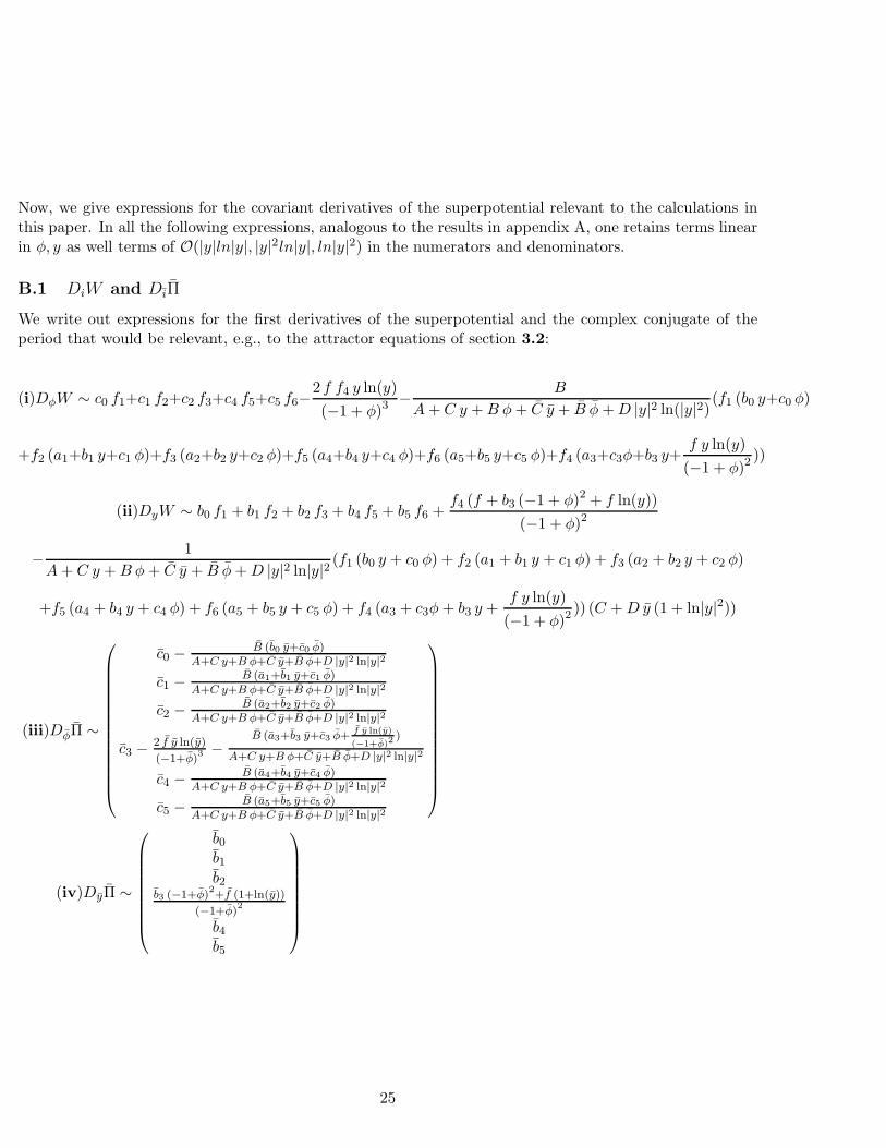
B.1 DiW and DiΠ

We write out expressions for the first derivatives of the superpotential and the complex conjugate of theperiod that would be relevant, e.g., to the attractor equations of section 3.2:

(i)DφW ∼ c0 f1+c1 f2+c2 f3+c4 f5+c5 f6−2 f f4 y ln(y)

(−1 + φ)3− B

A+C y +B φ+ C y + B φ+D |y|2 ln(|y|2) (f1 (b0 y+c0 φ)

+f2 (a1+b1 y+c1 φ)+f3 (a2+b2 y+c2 φ)+f5 (a4+b4 y+c4 φ)+f6 (a5+b5 y+c5 φ)+f4 (a3+c3φ+b3 y+f y ln(y)

(−1 + φ)2))

(ii)DyW ∼ b0 f1 + b1 f2 + b2 f3 + b4 f5 + b5 f6 +f4 (f + b3 (−1 + φ)2 + f ln(y))

(−1 + φ)2

− 1

A+ C y +B φ+ C y + B φ+D |y|2 ln|y|2 (f1 (b0 y + c0 φ) + f2 (a1 + b1 y + c1 φ) + f3 (a2 + b2 y + c2 φ)

+f5 (a4 + b4 y + c4 φ) + f6 (a5 + b5 y + c5 φ) + f4 (a3 + c3φ+ b3 y +f y ln(y)

(−1 + φ)2)) (C +D y (1 + ln|y|2))

(iii)DφΠ ∼

c0 − B (b0 y+c0 φ)A+C y+B φ+C y+B φ+D |y|2 ln|y|2

c1 − B (a1+b1 y+c1 φ)A+C y+B φ+C y+B φ+D |y|2 ln|y|2

c2 − B (a2+b2 y+c2 φ)A+C y+B φ+C y+B φ+D |y|2 ln|y|2

c3 − 2 f y ln(y)

(−1+φ)3 −

B (a3+b3 y+c3 φ+f y ln(y)

(−1+φ)2)

A+C y+B φ+C y+B φ+D |y|2 ln|y|2

c4 − B (a4+b4 y+c4 φ)A+C y+B φ+C y+B φ+D |y|2 ln|y|2

c5 − B (a5+b5 y+c5 φ)A+C y+B φ+C y+B φ+D |y|2 ln|y|2

(iv)DyΠ ∼

b0b1b2

b3 (−1+φ)2+f (1+ln(y))

(−1+φ)2

b4b5

25

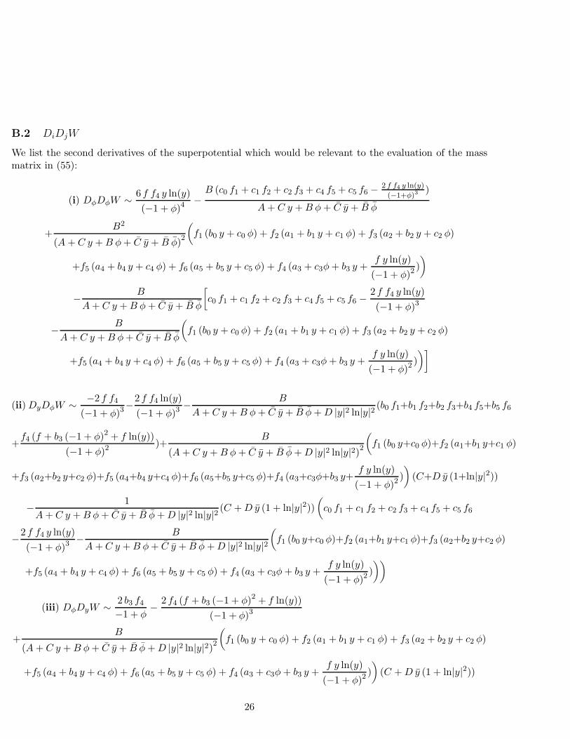
B.2 DiDjW

We list the second derivatives of the superpotential which would be relevant to the evaluation of the massmatrix in (55):

(i) DφDφW ∼ 6 f f4 y ln(y)

(−1 + φ)4−B (c0 f1 + c1 f2 + c2 f3 + c4 f5 + c5 f6 − 2 f f4 y ln(y)

(−1+φ)3)

A+ C y +B φ+ C y + B φ

+B2

(A+ C y +B φ+ C y + B φ)2

(

f1 (b0 y + c0 φ) + f2 (a1 + b1 y + c1 φ) + f3 (a2 + b2 y + c2 φ)

+f5 (a4 + b4 y + c4 φ) + f6 (a5 + b5 y + c5 φ) + f4 (a3 + c3φ+ b3 y +f y ln(y)

(−1 + φ)2)

)

− B

A+ C y +B φ+ C y + B φ

[

c0 f1 + c1 f2 + c2 f3 + c4 f5 + c5 f6 −2 f f4 y ln(y)

(−1 + φ)3

− B

A+ C y +B φ+ C y + B φ

(

f1 (b0 y + c0 φ) + f2 (a1 + b1 y + c1 φ) + f3 (a2 + b2 y + c2 φ)

+f5 (a4 + b4 y + c4 φ) + f6 (a5 + b5 y + c5 φ) + f4 (a3 + c3φ+ b3 y +f y ln(y)

(−1 + φ)2)

)]

(ii)DyDφW ∼ −2 f f4

(−1 + φ)3−2 f f4 ln(y)

(−1 + φ)3− B

A+ C y +B φ+ C y + B φ+D |y|2 ln|y|2 (b0 f1+b1 f2+b2 f3+b4 f5+b5 f6

+f4 (f + b3 (−1 + φ)2 + f ln(y))

(−1 + φ)2)+

B

(A+ C y +B φ+ C y + B φ+D |y|2 ln|y|2)2(

f1 (b0 y+c0 φ)+f2 (a1+b1 y+c1 φ)

+f3 (a2+b2 y+c2 φ)+f5 (a4+b4 y+c4 φ)+f6 (a5+b5 y+c5 φ)+f4 (a3+c3φ+b3 y+f y ln(y)

(−1 + φ)2)

)

(C+D y (1+ln|y|2))

− 1

A+ C y +B φ+ C y + B φ+D |y|2 ln|y|2 (C +D y (1 + ln|y|2))(

c0 f1 + c1 f2 + c2 f3 + c4 f5 + c5 f6

−2 f f4 y ln(y)

(−1 + φ)3− B

A+C y +B φ+ C y + B φ+D |y|2 ln|y|2(

f1 (b0 y+c0 φ)+f2 (a1+b1 y+c1 φ)+f3 (a2+b2 y+c2 φ)

+f5 (a4 + b4 y + c4 φ) + f6 (a5 + b5 y + c5 φ) + f4 (a3 + c3φ+ b3 y +f y ln(y)

(−1 + φ)2)

))

(iii) DφDyW ∼ 2 b3 f4

−1 + φ− 2 f4 (f + b3 (−1 + φ)2 + f ln(y))

(−1 + φ)3

+B

(A+ C y +B φ+ C y + B φ+D |y|2 ln|y|2)2(

f1 (b0 y + c0 φ) + f2 (a1 + b1 y + c1 φ) + f3 (a2 + b2 y + c2 φ)

+f5 (a4 + b4 y + c4 φ) + f6 (a5 + b5 y + c5 φ) + f4 (a3 + c3φ+ b3 y +f y ln(y)

(−1 + φ)2)

)

(C +D y (1 + ln|y|2))

26

− 1

(A+ C y +B φ+ C y + B φ+D |y|2 ln|y|2)2(

c0 f1+c1 f2+c2 f3+c4 f5+c5 f6−2 f f4 y ln(y)

(−1 + φ)3

)

(C+D y (1+ln|y|2))

− B

A+ C y +B φ+ C y + B φ+D |y|2 ln|y|2(

b0 f1+b1 f2+b2 f3+b4 f5+b5 f6+f4 (f + b3 (−1 + φ)2 + f ln(y))

(−1 + φ)2

− 1

A+ C y +B φ+ C y + B φ+D |y|2 ln|y|2(

f1 (b0 y + c0 φ) + f2 (a1 + b1 y + c1 φ) + f3 (a2 + b2 y + c2 φ)

+f5 (a4 + b4 y + c4 φ) + f6 (a5 + b5 y + c5 φ) + f4 (a3 + c3φ+ b3 y +f y ln(y)

(−1 + φ)2)

)

(C +D y (1 + ln|y|2)))

(iv)DyDyW ∼ f f4

y (−1 + φ)2− D

y (A+ C y +B φ+ C y + B φ+D |y|2 ln|y|2) y[

f1 (b0 y+c0 φ)+f2 (a1+b1 y+c1 φ)

+f3 (a2 + b2 y + c2 φ) + f5 (a4 + b4 y + c4 φ) + f6 (a5 + b5 y + c5 φ) + f4 (a3 + c3φ+ b3 y +f y ln(y)

(−1 + φ)2)

]

−(b0 f1 + b1 f2 + b2 f3 + b4 f5 + b5 f6 + f4 (f+b3 (−1+φ)2+f ln(y))

(−1+φ)2) (C +D y (1 + ln|y|2))

A+ C y +B φ+ C y + B φ+D |y|2 ln|y|2

+1

(A+ C y +B φ+ C y + B φ+D |y|2 ln|y|2)2[

f1 (b0 y + c0 φ) + f2 (a1 + b1 y + c1 φ) + f3 (a2 + b2 y + c2 φ

+f5 (a4 + b4 y + c4 φ) + f6 (a5 + b5 y + c5 φ) + f4 (a3 + c3φ+ b3 y +f y ln(y)

(−1 + φ)2)

]

(C +D y (1 + ln|y|2))2

− 1

A+ C y +B φ+ C y + B φ+D |y|2 ln|y|2 (C +D y (1 + ln|y|2))[

b0 f1 + b1 f2 + b2 f3 + b4 f5 + b5 f6

+f4 (f + b3 (−1 + φ)2 + f ln(y))

(−1 + φ)2− 1

A+ C y +B φ+ C y + B φ+D |y|2 ln|y|2(

f1 (b0 y+c0 φ)+f2 (a1+b1 y+c1 φ)

+f3 (a2+b2 y+c2 φ)+f5 (a4+b4 y+c4 φ)+f6 (a5+b5 y+c5 φ)+f4 (a3+c3φ+b3 y+f y ln(y)

(−1 + φ)2)

)

(C+D y (1+ln|y|2))]

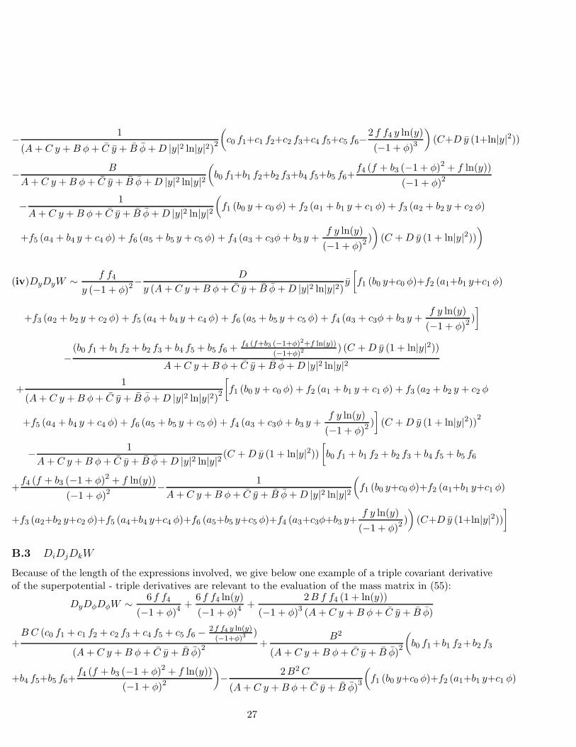
B.3 DiDjDkW

Because of the length of the expressions involved, we give below one example of a triple covariant derivativeof the superpotential - triple derivatives are relevant to the evaluation of the mass matrix in (55):

DyDφDφW ∼ 6 f f4

(−1 + φ)4+

6 f f4 ln(y)

(−1 + φ)4+

2B f f4 (1 + ln(y))

(−1 + φ)3 (A+ C y +B φ+ C y + B φ)

+BC (c0 f1 + c1 f2 + c2 f3 + c4 f5 + c5 f6 − 2 f f4 y ln(y)

(−1+φ)3)

(A+ C y +B φ+ C y + B φ)2 +

B2

(A+ C y +B φ+ C y + B φ)2

(

b0 f1 +b1 f2 +b2 f3

+b4 f5+b5 f6+f4 (f + b3 (−1 + φ)2 + f ln(y))

(−1 + φ)2

)

− 2B2C

(A+ C y +B φ+ C y + B φ)3

(

f1 (b0 y+c0 φ)+f2 (a1+b1 y+c1 φ)

27

+f3 (a2 + b2 y + c2 φ) + f5 (a4 + b4 y + c4 φ) + f6 (a5 + b5 y + c5 φ) + f4 (a3 + c3φ+ b3 y +f y ln(y)

(−1 + φ)2)

)

− B

A+ C y +B φ+ C y + B φ

( −2 f f4

(−1 + φ)3−2 f f4 ln(y)

(−1 + φ)3−B (b0 f1 + b1 f2 + b2 f3 + b4 f5 + b5 f6 + f4 (f+b3 (−1+φ)2+f ln(y))

(−1+φ)2)

A+ C y +B φ+ C y + B φ

+BC

(A+ C y +B φ+ C y + B φ)2

(

f1 (b0 y + c0 φ) + f2 (a1 + b1 y + c1 φ) + f3 (a2 + b2 y + c2 φ)

+f5 (a4 + b4 y + c4 φ) + f6 (a5 + b5 y + c5 φ) + f4 (a3 + c3φ+ b3 y +f y ln(y)

(−1 + φ)2)

)

)

+(C +D y (1 + ln|y|2))

A+ C y +B φ+ C y + B φ) (A +C y +B φ+ C y + B φ+D |y|2 ln|y|2)

(

BC (c0 f1+c1 f2+c2 f3+c4 f5+c5 f6

−2 f f4 y ln(y)

(−1 + φ)3− B

A+ C y +B φ+ C y + B φ+D|y|2ln|y|2(

f1 (b0 y + c0 φ) + f2 (a1 + b1 y + c1 φ)

+f3 (a2 + b2 y + c2 φ) + f5 (a4 + b4 y + c4 φ) + f6 (a5 + b5 y + c5 φ) + f4 (a3 + c3φ+ b3 y +f y ln(y)

(−1 + φ)2)

))

−[

6 f f4 y ln(y)

(−1 + φ)4−B (c0 f1 + c1 f2 + c2 f3 + c4 f5 + c5 f6 − 2 f f4 y ln(y)

(−1+φ)3)

A+ C y +B φ+ C y + B φ+

B2

(A+ C y +B φ+ C y + B φ)2

(

f1 (b0 y+c0 φ)

+f2 (a1+b1 y+c1 φ)+f3 (a2+b2 y+c2 φ)+f5 (a4+b4 y+c4 φ)+f6 (a5+b5 y+c5 φ)+f4 (a3+c3φ+b3 y+f y ln(y)

(−1 + φ)2)

)

−(B (c0 f1 + c1 f2 + c2 f3 + c4 f5 + c5 f6 −2 f f4 y ln(y)

(−1 + φ)3− B

A+ C y +B φ+ C y + B φ

(

f1 (b0 y + c0 φ)

+f2 (a1+b1 y+c1 φ)+f3 (a2+b2 y+c2 φ)+f5 (a4+b4 y+c4 φ)+f6 (a5+b5 y+c5 φ)+f4 (a3+c3φ+b3 y+f y ln(y)

(−1 + φ)2)

)]

C The Complex Structure Moduli Space Metric (Inverse) and Its Deriva-tives Near the Conifold Locus

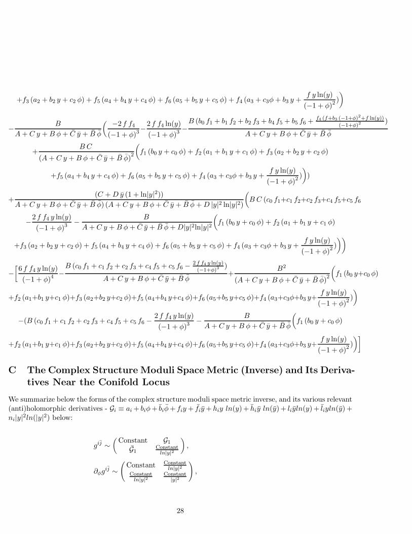
We summarize below the forms of the complex structure moduli space metric inverse, and its various relevant(anti)holomorphic derivatives - Gi ≡ ai + biφ+ biφ+ fiy+ fiy+ hiy ln(y) + hiy ln(y) + liyln(y) + liyln(y) +ni|y|2ln(|y|2) below:

gij ∼(

Constant G1

G1Constantln|y|2

)

,

∂φgij ∼

(

Constant Constantln|y|2

Constantln|y|2

Constant|y|2

)

,

28

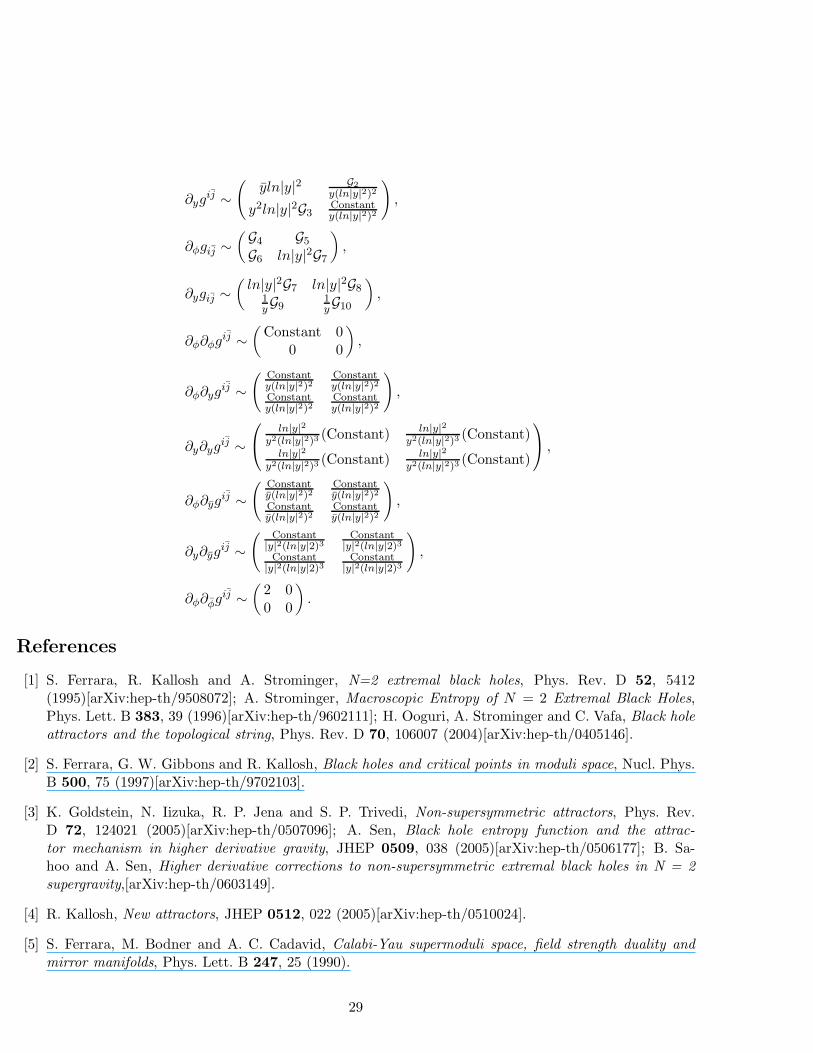
∂ygij ∼

(

yln|y|2 G2y(ln|y|2)2

y2ln|y|2G3Constanty(ln|y|2)2

)

,

∂φgij ∼(G4 G5

G6 ln|y|2G7

)

,

∂ygij ∼(

ln|y|2G7 ln|y|2G81yG9

1yG10

)

,

∂φ∂φgij ∼

(

Constant 00 0

)

,

∂φ∂ygij ∼

( Constanty(ln|y|2)2

Constanty(ln|y|2)2

Constanty(ln|y|2)2

Constanty(ln|y|2)2

)

,

∂y∂ygij ∼

ln|y|2

y2(ln|y|2)3(Constant) ln|y|2

y2(ln|y|2)3(Constant)

ln|y|2

y2(ln|y|2)3(Constant) ln|y|2

y2(ln|y|2)3(Constant)

,

∂φ∂ygij ∼

( Constanty(ln|y|2)2

Constanty(ln|y|2)2

Constanty(ln|y|2)2

Constanty(ln|y|2)2

)

,

∂y∂ygij ∼

( Constant|y|2(ln|y|2)3

Constant|y|2(ln|y|2)3

Constant|y|2(ln|y|2)3

Constant|y|2(ln|y|2)3

)

,

∂φ∂φgij ∼

(

2 00 0

)

.

References

[1] S. Ferrara, R. Kallosh and A. Strominger, N=2 extremal black holes, Phys. Rev. D 52, 5412(1995)[arXiv:hep-th/9508072]; A. Strominger, Macroscopic Entropy of N = 2 Extremal Black Holes,Phys. Lett. B 383, 39 (1996)[arXiv:hep-th/9602111]; H. Ooguri, A. Strominger and C. Vafa, Black holeattractors and the topological string, Phys. Rev. D 70, 106007 (2004)[arXiv:hep-th/0405146].

[2] S. Ferrara, G. W. Gibbons and R. Kallosh, Black holes and critical points in moduli space, Nucl. Phys.B 500, 75 (1997)[arXiv:hep-th/9702103].

[3] K. Goldstein, N. Iizuka, R. P. Jena and S. P. Trivedi, Non-supersymmetric attractors, Phys. Rev.D 72, 124021 (2005)[arXiv:hep-th/0507096]; A. Sen, Black hole entropy function and the attrac-tor mechanism in higher derivative gravity, JHEP 0509, 038 (2005)[arXiv:hep-th/0506177]; B. Sa-hoo and A. Sen, Higher derivative corrections to non-supersymmetric extremal black holes in N = 2supergravity,[arXiv:hep-th/0603149].

[4] R. Kallosh, New attractors, JHEP 0512, 022 (2005)[arXiv:hep-th/0510024].

[5] S. Ferrara, M. Bodner and A. C. Cadavid, Calabi-Yau supermoduli space, field strength duality andmirror manifolds, Phys. Lett. B 247, 25 (1990).

29

[6] M. Alishahiha and H. Ebrahim, New attractor, entropy function and black hole partition function,arXiv:hep-th/0605279.

[7] A. Giryavets, New attractors and area codes, JHEP 0603, 020 (2006)[arXiv:hep-th/0511215].

[8] P. Candelas, X. C. De La Ossa, P. S. Green and L. Parkes, A Pair Of Calabi-Yau Manifolds As AnExactly Soluble Superconformal Theory, Nucl. Phys. B 359, 21 (1991); P. Candelas, X. De La Ossa,A. Font, S. Katz and D. R. Morrison, Mirror symmetry for two parameter models. I, Nucl. Phys. B416, 481 (1994)[arXiv:hep-th/9308083].

[9] A. Giryavets, S. Kachru, P. K. Tripathy and S. P. Trivedi, Flux compactifications on Calabi-Yau three-folds, JHEP 0404, 003 (2004)[arXiv:hep-th/0312104].

[10] A. Misra and A. Nanda, Flux vacua statistics for two-parameter Calabi-Yau’s, Fortsch. Phys. 53, 246(2005) [arXiv:hep-th/0407252].

[11] P. K. Tripathy and S. P. Trivedi, Non-supersymmetric attractors in string theory, JHEP 0603, 022(2006) [arXiv:hep-th/0511117].

[12] J. Gray, Y. H. He, V. Jejjala and B. D. Nelson, Exploring the vacuum geometry of N = 1 gauge theories,[arXiv:hep-th/0604208].

[13] A. Chou, R. Kallosh, J. Rahmfeld, S. J. Rey, M. Shmakova and W. K. Wong, Critical points and phasetransitions in 5d compactifications of M-theory, Nucl. Phys. B 508 (1997) 147 [arXiv:hep-th/9704142].

[14] G. W. Moore, Arithmetic and attractors, arXiv:hep-th/9807087.

[15] G. W. Moore, Les Houches lectures on strings and arithmetic, arXiv:hep-th/0401049.

[16] J. Gray, Y. H. He and A. Lukas, Algorithmic algebraic geometry and flux vacua, arXiv:hep-th/0606122.

30