On the efficient calculation of van Rossum distances

On the efficient calculation of van Rossumdistances.

Conor Houghton1,2∗and Thomas Kreuz3†

1 School of Mathematics, Trinity College Dublin, Ireland.2 Department of Computer Science, University of Bristol, England.

3 Institute for complex systems - CNR, Sesto Fiorentino, Italy

March 3, 2012

Abstract

The van Rossum metric measures the distance between two spiketrains. Measuring a single van Rossum distance between one pair ofspike trains is not a computationally expensive task, however, manyapplications require a matrix of distances between all the spike trainsin a set or the calculation of a multi-neuron distance between twopopulations of spike trains. Moreover, often these calculations needto be repeated for many different parameter values. An algorithm ispresented here to render these calculation less computationally expen-sive, making the complexity linear in the number of spikes rather thanquadratic.

Introduction

The van Rossum metric is used to calculate a distance between two spiketrains (van Rossum, 2001). It has been shown to be a good metric in thesense that the distance between multiple responses to the same stimulus istypically smaller than the distance between responses to different stimuli

∗[email protected]†[email protected]

1

(Machens et al., 2003; Narayan et al., 2006). Like some other spike traindistances (Victor and Purpura, 1996), the van Rossum metric depends on aparameter τ which determines the time scale in the spike trains to which themetric is sensitive. In the τ → ∞ limit of the parameter range the metricmeasures the difference in spike numbers while in the other limit, whereτ = 0, it counts non-coincident spikes.

If the two spike trains have roughly the same number of spikes, n say,then the complexity of the calculation of the van Rossum metric is of or-der n2. Often an entire distance matrix is required containing the pairwisedistances between all the spike trains in a set. This is needed, for example,when calculating a preferred value of the time scale τ : the standard methodinvolves metric clustering and this requires the calculation of a distance ma-trix for multiple values of the time scale (Victor and Purpura, 1996; Machenset al., 2003; Wohlgemuth and Ronacher, 2007; Narayan et al., 2006; Toupset al., 2011). The optimal time scale is sometimes interpreted as indicativetime scale for the temporal precision in coding. Although this interpretationshould be treated with some caution (Chicharro et al., 2011), the optimaltime scale is nonetheless useful as a way of maximizing the performance ofthe metric in applications. If there are N spike trains in the set, calculatingthe van Rossum distance matrix is, at face value, an order N2n2 calculation.For large data sets this can be a considerable computational burden.

The same holds true for a number of variations of the van Rossum met-ric such as the synapse-like metric introduced in (Houghton, 2009) and themulti-neuron metric (Houghton and Sen, 2008). The latter is designed toestimate the distance between two sets of neuronal population responses andis particularly troublesome from the point of view of computational expense.

Here, a trick is presented to reduce the computational cost for all threeof these cases: For the regular van Rossum distance between two spike trainsof length n the cost is reduced from order n2 to order n and, hence, thecost of calculating a matrix of distances for N such spike trains from orderN2n2 to order N2n. The same speed-up is obtained for the van Rossum-like metrics. Similarly, in the multi-neuron case the cost of calculating thedistance between two populations of P spike trains each will be reduced fromorder P 2n2 to order P 2n.

2

Methods

The van Rossum metric

To describe the van Rossum distance it is useful to first define a map fromspike trains to functions: given a spike train

u = {u1, u2, · · · , un} (1)

it is mapped to f(t;u) by filtering it with a kernel h(t):

u 7→ f(t;u) =n∑

i=1

h(t− ui). (2)

The kernel function has to be specified, here, as in (van Rossum, 2001), thecausal exponential is used

h(t) =

{0 t < 0e−t/τ t ≥ 0

. (3)

The decay constant τ is the time scale which parameterizes the metric.The van Rossum metric is induced on the space of spike trains by the L2

metric on the space of functions. In other words, the distance between twospike trains u and v is given by

d(u,v; τ) =

√2

τ

∫ ∞

0

dt[f(t;u)− f(t;v)]2. (4)

where the normalizing factor of 2/τ is included so that there is a distance ofone between a spike train with a single spike and one with no spikes. In fact,for the causal exponential filter this integral can be done explicitly to give adistance (Schrauwen and Van Campenhout, 2007; Paiva et al., 2009)

[d(u,v; τ)]2 =∑i,j

e−|ui−uj |/τ +∑i,j

e−|vi−vj |/τ

−2∑i,j

e−|ui−vj |/τ . (5)

Now, the trick relies on the calculation of an extra vector for each spiketrain in the set; this extra vector will be called the markage vector. Given a

3

spike train u, the markage vectorm(u) will have the same number of elementas there are spikes, so #(m(u))=#(u). The entries in the markage vectorare defined recursively so that m1 = 0 and

mi = (mi−1 + 1)e−(ui−ui−1)/τ . (6)

This meansmi =

∑j|ui>uj

e−(ui−uj)/τ (7)

where j|ui > uj indicates that the sum is restricted to values of j whereuj < ui. In fact, it will be assumed here that the spike times are in ascendingorder, which in most real situations they will be; this means that j|ui >uj is actually equivalent to j < i. However, note that this notation forrestricted values of an index is used below in other contexts where it can notbe simplified in this way. Also, when needed for clarity the notation mi(u)will be used for the ith component of m(u), but in the above, the argumenthas been left out for brevity. The function f(t) is discontinuous and mi isequal to the left limit of f(t) at ui:

mi = f(ui−) = limt→ui−

f(t). (8)

The idea is to use the markage vector to reduce the double sums in theexpression for d(u,v), Eq. 5, to single sums. For convenience this equationis first rewritten to avoid the use of the absolute value

[d(u,v; τ)]2 =n1 + n2

2+∑i

∑j|ui>uj

e−(ui−uj)/τ +∑i

∑j|vi>vj

e−(vi−vj)/τ

−∑i

∑j|ui>vj

e−(ui−vj)/τ −∑i

∑j|vi>uj

e−(vi−uj)/τ (9)

where n1 = #(u) and n2 = #(v) are the number of spikes in the two spiketrains. This yields ∑

i

∑j|ui>uj

e−(ui−uj)/τ =∑i

mi(u). (10)

The cross-like terms are trickier, let J(i) denote the index of the last spiketime in v that is earlier than ui, hence

J(i) = max (j|ui > vj), (11)

4

which leads to∑i

∑j|ui>vj

e−(ui−vj)/τ =∑i

e−(ui−vJ(i))/τ∑

j|vJ(i)≥vj

e−(vJ(i)−vj)/τ

=∑i

e−(ui−vJ(i))/τ

1 +∑

j|vJ(i)>vj

e−(vJ(i)−vj)/τ

=

∑i

e−(ui−vJ(i))/τ[1 +mJ(i)(v)

]. (12)

Since the other two terms in the expression for d(u,v) are identical to thetwo above with u and v switched they can be calculated in the same way,so, for example,∑

i

∑j|vi>uj

e−(vi−uj)/τ =∑i

e−(vi−uK(i))/τ[1 +mK(i)(u)

]. (13)

where K(i) = max (j|vi > uj), the analog of J(i) with u and v switched.For time ordered spike trains, this reduces the calculation of all four

terms from n2 to n. The two cross terms, containing times from both uand v are the most important since when calculating a distance matrix theseare the most expensive, involving N2n2 calculations without markage, thetwo square terms need only be calculated once for each spike train and aretherefore linear in N .

Using the markage vector does introduce extra calculations. Along withthe calculation of the markage vector itself, there is the need to calculateJ(i), the index of the time on one spike train immediately prior to the ithtime in the other. If the spike trains were not time ordered this calculationwould be order n2; however, for the more biologically relevant case of timeordered spike trains, J(i) can be calculated iteratively by advancing it fromits previous value when necessary. It is seen below that the constant prefactorto N2n in the algorithm with markage is larger than the prefactor to N2n2 inthe traditional algorithm, but that it is worthwhile using the new algorithmeven for quite short spike trains.

Other van Rossum-like metrics

There are a number of variations of the van Rossum metrics. One generaliza-tion is to consider other kernels. In the standard formulation the kernel h(t)

5

is a causal exponential, Eq. 3, but other kernels can be used: a square pulseor normal curve are popular alternatives. It is also possible to regard theexponential factors in the integrated formula, Eq. 5 as kernels and replacethese with other functions (Schrauwen and Van Campenhout, 2007). Thealgorithm proposed here will not, in general, be useful for these other cases.It might be possible to generalize the sum formula for the markage, Eq. 7,but this is an order n2 calculation and would contribute Nn2 to the overallcalculation of a distance matrix. In the causal exponential case consideredhere there is also an iterative formula for the markage, Eq. 6. This will notwork for all choices of kernel.

There is, however, another generalization of the van Rossum metric inwhich the map from spike trains to functions is viewed as a differential equa-tion, rather than as a filtering. In this description, u is mapped to f(t;u)where

τdf

dt= −f (14)

with discontinuitiesf(ui+) = f(ui−) + 1 (15)

at the spikes. The synapse-like metric introduced in (Houghton, 2009) changesthe map from spike trains to functions in order that it mimics aspects of thesynaptic conductivity. Specifically, it accounts for the depletion of availablebinding sites by changing how much f is increased by each spike; f(t;u) isdefined as the solution to the differential equation

τd

dtf = −f

f(ui+) = (1− µ)f(ui−) + 1 (16)

at the spike times ui. The first parameter τ , as before, is a time scale,associated with the precision of spiking, while the second parameter µ reflectsa reduction of the significance of spike timing in spike clusters.

To calculate the integrated form of this distance it is convenient to firstdefine an increment vector δ(u), where δ1 = 1 and

δi = 1− µ∑

j|ui>uj

δie−(ui−uj)/τ . (17)

The quantity δi is equal to the increment in f(t;u) at ui. Now, letting

6

α = δ(u) and β = δ(v) the synapse distance is

d(u,v) =∑i,j

αiαje−|ui−uj |/τ +

∑i,j

βiβje−|vi−vj |/τ

−2∑i,j

αiβje−|ui−vj |/τ . (18)

Again, this calculation can be made more efficient using a markage vector;this time it will have the form

mi =∑

j|ui>uj

δie−(ui−uj)/τ . (19)

The markage and increment vector can be calculated iteratively in leap-frogfashion

mi = (mi−1 + δi−1)e−(ui−ui−1)/τ

δi = 1− µmi. (20)

For example,∑i,j

αiαje−|ui−uj |/τ =

∑i

α2i + 2

∑i

αi

∑j|ui>uj

αje−|ui−uj |/τ

=∑i

αi(αi + 2mi) (21)

with similar expressions for the other terms; in short, the formulae for theefficient calculation of the synapse metric only differ from formulae for theoriginal van Rossum metric in the inclusion of the components of the incre-ment vector.

The multi-neuron van Rossum metric

There is also a multi-neuron van Rossum metric (Houghton and Sen, 2008)which was proposed as tool for quantifying if and how populations of neuronscooperate to encode a sensory input. Here, computational expense is an evenmore acute problem but the same trick can be used.

In this setup there are two population responses, each with P spike trains:U = {u1,u2, . . . ,uP} and V = {u1,u2, . . . ,uP}. Spikes are represented as

7

upi and vqj with i = 1, .., np

u and j = 1, .., nqv where np

u and nqv denote the

numbers of spikes in the pth and qth spike train of the populations U and V ,respectively. By locating the P spike trains of the two population responsesU and V in a space of vector fields, with a different unit vector assigned toeach neuron, interpolation between the two extremes, the labeled line (LL)coding and the summed population (SP) coding, is achieved by varying theangle θ between unit vectors from zero (SP) to π/2 (LL) or, equivalently, theparameter c = cos θ from one to zero:

d(U ,V ; τ) =

√√√√2

τ

∑p

(∫ ∞

0

|δp|2dt+ c∑q =p

∫ ∞

0

δpδqdt

)(22)

with δp = f(t,up)− f(t,vp).In the original description in (Houghton and Sen, 2008) the metric is

described in terms of the unit vectors corresponding to each neuron in thepopulation. In the formula above the dot-products between the unit vectorshave already been performed, giving a simpler formula.

Similar to the single-neuron case (Schrauwen and Van Campenhout, 2007;Paiva et al., 2009) the multi-neuron van Rossum distance can also be esti-mated in a more efficient way by integrating analytically:

d(U ,V ; τ) =

√√√√∑p

(Rp + c

∑q =p

Rpq

)(23)

with

Rp =∑i,j

e−|upi−up

j |/τ +∑i,j

e−|vpi −vpj |/τ − 2∑i,j

e−|upi−vpj |/τ (24)

being the bivariate single neuron distance, as in Eq. 5, between the p-thspike trains of u and v and

Rpq =∑i,j

e−|upi−uq

j |/τ +∑i,j

e−|vpi −vqj |/τ −∑i,j

e−|upi−vqj |/τ −

∑i,j

e−|vpi −uqj |/τ (25)

representing the cross-neuron terms that are needed to fully capture theactivity of the pooled population. As in the estimate in Eq. 22 the variablec interpolates between the labeled line and the summed population distance.

8

These are the two equations for which the markage trick can be appliedsince all of these sums of exponentials can be rewritten using markage vectorsin the same way as it was done in Eqs. 9, 10, and 12, so, taking the firstterm in Rpq as an example∑

i,j

e−|upi−uq

j |/τ =∑i

e−(upi−uq

J(i))/τ [1 +mJ(i)(u

q)]

+∑i

e−(uqi−up

J(i))/τ [1 +mJ(i)(u

p)]

(26)

In case of τ = ∞ Eq. 23 remains still valid, however, the calculation ofthe contributing terms simplifies to

Rp = npu(n

pu − np

v) + npv(n

pv − np

u) (27)

and

Rpq = npu(n

qu − nq

v) + nqu(n

pu − np

v) + npv(n

qv − nq

u) + nqv(n

pv − np

u). (28)

If τ = ∞ and c = 1, the calculation of the population van Rossum distanceD simplifies even further:

D(u,v; τ) =√R (29)

with

R =P∑

p=1

npu

P∑p=1

(npu − np

v) +N∑p=1

npv

P∑p=1

(npv − np

u). (30)

There is a generalization of this metric in which there are many differentangles, or equivalently, many different c parameters; this allows each pairof neurons to lie on a different point in the interpolation between summedcoding and labeled coding (Houghton and Sen, 2008). The simplificationsdiscussed here can also be applied in this case.

Results

The algorithm of the regular van Rossum metric was tested using simulatedspike trains. The spike trains were generated as a homogeneous Poisson pro-cess with rate 30Hz. The algorithm (with the timescale set to τ = 12ms)

9

0

0.1

0.2

0.3

0.4

0.5

0.6

0 1 2 3 4 5 6 7 8

T[s]

L [s]

traditionalmarkage

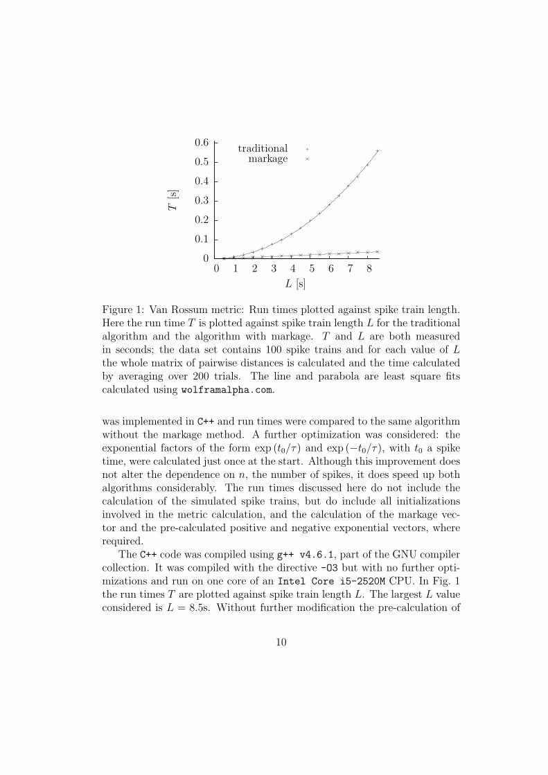
Figure 1: Van Rossum metric: Run times plotted against spike train length.Here the run time T is plotted against spike train length L for the traditionalalgorithm and the algorithm with markage. T and L are both measuredin seconds; the data set contains 100 spike trains and for each value of Lthe whole matrix of pairwise distances is calculated and the time calculatedby averaging over 200 trials. The line and parabola are least square fitscalculated using wolframalpha.com.

was implemented in C++ and run times were compared to the same algorithmwithout the markage method. A further optimization was considered: theexponential factors of the form exp (t0/τ) and exp (−t0/τ), with t0 a spiketime, were calculated just once at the start. Although this improvement doesnot alter the dependence on n, the number of spikes, it does speed up bothalgorithms considerably. The run times discussed here do not include thecalculation of the simulated spike trains, but do include all initializationsinvolved in the metric calculation, and the calculation of the markage vec-tor and the pre-calculated positive and negative exponential vectors, whererequired.

The C++ code was compiled using g++ v4.6.1, part of the GNU compilercollection. It was compiled with the directive -O3 but with no further opti-mizations and run on one core of an Intel Core i5-2520M CPU. In Fig. 1the run times T are plotted against spike train length L. The largest L valueconsidered is L = 8.5s. Without further modification the pre-calculation of

10

exponentials would be problematic for longer spike trains since exp (t0/τ)will be too large to store as a double.

The graph in Fig. 1 shows both the recorded run times and a least squaresfit to a parabola, for the traditional algorithm, and to a line for the algorithmwith markage. For the algorithms with exponential pre-calculation shown inthe graphs the best-fit curves are

T0(L) = 0.00738L2 + 0.00209L+ 0.00145 (31)

for the traditional algorithm and

T1(L) = 0.00432L− 0.00011 (32)

for the algorithm with markage. Of course, the run times depend on platform,hardware and implementation, but the ratio should give an approximateindication of how well the algorithm performs

T1 =0.58

LT0 +O(1) (33)

or, in terms of spike number, n,

T1 ≈17.4

nT0 (34)

for larger values of n. The factor 17.4 can be thought of as an overhead,so for a collection of spike trains with an average of 174 spikes in each, thespeed up will be tenfold. The implication for the equation is that that thenew algorithm is worth using when there are more than 17.4 spikes, in fact,for small values of n the quadratic is a poor fit and T0 = 0.00214 for L = 0.5s,equivalent to n = 15, while T1(0.5) = 0.00329, so the traditional algorithmis still considerably slower.

Exponential pre-calculation has a more substantial effect on the tradi-tional algorithm than on the algorithm with markage; the traditional algo-rithm requires many more exponential factors. Fitting curves to the runtimes without exponential pre-calculation gives

T0(L) = 0.219L2 + 0.00496L+ 0.00135 (35)

for the traditional algorithm and

T1(L) = 0.0185L− 0.000433 (36)

11

for the markage algorithm, so

T1 =0.084

LT0 +O(1) ≈ 2.5

nT0. (37)

The ratio between the markage algorithm with exponential pre-calculationand the traditional algorithm without is 0.6/n. Varying N , the number ofspike trains, verifies that the run times have an N2 dependence.

If the same analysis is applied to the synapse metric with exponentialpre-calculation and with µ = 0.5, we obtain

T1 ≈15.3

nT0. (38)

The multi-neuron metric was also studied; using P = 10, N = 20 and cos θ =0.5 yielded

T1 ≈18.0

nT0. (39)

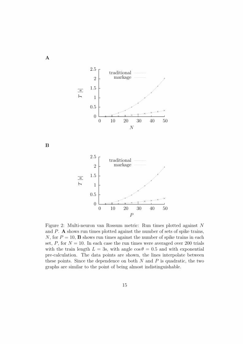
In Fig. 2 the running time for the multi-neuron metric is plotted against Nand P , the number of sets of spike trains and the number of spike trains ineach set. In each case, again considerably smaller run times are observed forthe algorithm with markage.

Discussion

The algorithms described here are more complicated to implement than themore straight-forward approaches; however, for large spike trains the speedup is considerable and may make practical an analysis technique that wouldnot otherwise be quick enough to be useful.

Although the method presented here is a computational trick, it is in-teresting to note that a biologically inspired quantity, like the van Rossummetric and its multi-neuron extension, might be expected to permit a trickof this sort. The trick works by replacing a sum over history by a runningtally; this sort of replacement is typical of biological systems.

Matlab1 and c++ 2 source codes for both the regular and the multi-neuronvan Rossum distances are available.

1http://www.fi.isc.cnr.it/users/thomas.kreuz/sourcecode.html2http://sourceforge.net/p/spikemetrics

12

Acknowledgements

We gratefully acknowledge useful discussions with Daniel Chicharro. CHis grateful to the James S McDonnell Foundation for a Scholar Award inUnderstanding Human Cognition. We thank one of the anonymous referee’sfor suggesting the pre-calculation of the exponentials.

References

Chicharro D, Kreuz T, Andrzejak RG. 2011. What can spike train distancestell us about the neural code? Journal of Neuroscience Methods 199:146–165.

Houghton C. 2009. Studying spike trains using a van Rossum metric with asynapses-like filter. Journal of Computational Neuroscience 26:149–155.

Houghton C, Sen K. 2008. A new multi-neuron spike-train metric. NeuralComputation 20:1495–1511.

Machens CK, Schutze H, Franz A, Kolesnikova O, Stemmler MB, RonacherB, Herz A. 2003. Single auditory neurons rapidly discriminate conspecificcommunication signals. Nature Neuroscience 6:341–2.

Narayan R, Grana G, Sen K. 2006. Distinct time scales in cortical dis-crimination of natural sounds in songbirds. Journal of Neurophysiology96:252–258.

Paiva ARC, Park I, Prıncipe JC. 2009. A reproducing kernel Hilbert spaceframework for spike train signal processing. Neural Computation 21:424–449.

Schrauwen B, Van Campenhout J. 2007 Linking non-binned spike trainkernels to several existing spike train metrics. Neurocomputing 70:1247–1253.

Toups JV, Fellous J-M, Thomas PJ, Sejnowski TJ, Tiesinga, PH. 2011. Find-ing the event structure of neuronal spike trains. Neural Computation23:2169–2208.

van Rossum M. 2001. A novel spike distance. Neural Computation 13:751–763.

Victor JD, Purpura KP. 1996. Nature and precision of temporal codingin visual cortex: a metric-space analysis. Journal of Neurophysiology76:1310–1326.

13

Wohlgemuth S, Ronacher B. 2007. Auditory discrimination of amplitudemodulations based on metric distances of spike trains. Journal of Neuro-physiology 97:3082–3092.

Declaration of interest

The authors report no conflicts of interest. The authors alone are responsiblefor the content and writing of the paper.

14

A

0

0.5

1

1.5

2

2.5

0 10 20 30 40 50

T[s]

N

traditionalmarkage

B

0

0.5

1

1.5

2

2.5

0 10 20 30 40 50

T[s]

P

traditionalmarkage

Figure 2: Multi-neuron van Rossum metric: Run times plotted against Nand P . A shows run times plotted against the number of sets of spike trains,N , for P = 10, B shows run times against the number of spike trains in eachset, P , for N = 10. In each case the run times were averaged over 200 trialswith the train length L = 3s, with angle cos θ = 0.5 and with exponentialpre-calculation. The data points are shown, the lines interpolate betweenthese points. Since the dependence on both N and P is quadratic, the twographs are similar to the point of being almost indistinguishable.

15