On the Causality Between Saving and Growth: Long- and ...128726/FULLTEXT01.pdf · On the Causality Between Saving and Growth: ... theory offers little guidance to the true nature

On the Causality Between Saving and Growth:

Long- and Short Run Dynamics and Country Heterogeneity∗

Björn Andersson�

Abstract

The temporal interdependence between saving and output has been in focus in a number ofrecent empirical studies. Results from these studies have compelled some authors to questionthe traditional notion of a causal chain where saving leads growth through capitalaccumulation. This paper contributes to this literature. As opposed to the previous studies,which have mainly utilised panel-estimation methods, the tests of causal chains here arecarried out in time-series settings. Saving and GDP are estimated in bivariate vectorautoregressive or vector error-correction models for Sweden, UK, and USA, and tests ofGranger non-causality are performed within the estimated systems. The main results show thatthe causal chains linking saving and output differ across countries, and also that causalityassociated with adjustments to long-run relations might go in different directions thancausality associated with short-term disturbances.

Keywords: saving; growth; Granger-causality; cointegration; VAR; VECMJEL classification: C32; E21; O40; O57

∗ This paper has benefitted greatly from comments and suggestions by Thomas Lindh, Sara Lindberg and seminarparticipants at the macroeconomic workshop at Uppsala University. Remaining errors are of course my own. I amalso indebted to Mikael Apel at the Swedish Central Bank for data provision.� Björn Andersson, Department of Economics, Uppsala University, P.O. Box 513, S-751 20 Uppsala, Sweden tel: +46 18 4717632, fax: +46 18 4711478, e-mail: [email protected]

1

1 Introduction

”…neither the proportion of income saved nor the rate of growth of productivity per man

(nor, of course, the rate of increase in population) are independent variables with respect to

the rate of increase in production;…” Kaldor (1960, p.259).

The close relationship between the saving rate of the economy and the growth rate is a stylised

feature which has been well documented in a number of empirical investigations. In fact, it is

one of the few, if not the only, relationship which can not be erased when other possible

growth influences are conditioned on1. This is a result which has been found in several

sensitivity analyses in the growth literature, e.g. Levine and Renelt (1992) and Sala-i-Martin

(1997). Although it is emphasised that no causality should be inferred from this positive

contemporaneous correlation, little is said about the causal links between the variables other

than that they most likely are jointly determined. The close connection between saving and

growth has also been a key finding in the empirical saving literature; the possibility that

country differences in saving rates could be explained by differences in growth rates was

recognised early.

Recently, a couple of articles have dealt with the question of the temporal interdependence

between the growth rate and the saving rate.2 These papers have looked more closely on what

theory predicts regarding the timing of movements of saving and growth, and to what extent

this is confirmed or rejected by empirical facts. The results from these studies have urged

some authors to call for a reinterpretation of the traditional notion of a growth-capital

accumulation relationship where capital accumulation supposedly leads growth. The present

paper is a contribution to this literature. Previous studies have mainly relied on cross-section

or panel data to examine the causal relationship. The point of departure here is to exploit time-

series features and the information contained in the long-run relationship between the

variables. Hence, saving and growth are modelled bivariately in vector autoregressive (VAR)

or vector error-correction (VEC) models for three countries - Sweden, UK, and USA - and

causality tests are then performed within these systems.

1 The saving rate and the investment rate are used almost interchangeably in this literature, often with reference tothe high degree of correlation between the variables. This paper focuses on the gross saving rate except whereindicated.2 See Carroll and Weil (1994), King and Levine (1994), Blomström, Lipsey, and Zejan (1996), Paxson (1996), Inand Doucouliagos (1997), Deaton (1997), Sinha and Sinha (1998), Vanhoudt (1998).

2

The main results are that the temporal relationship between saving and GDP differs across

countries. There is evidence of a causal chain linking higher saving to larger output but some

countries also have causality running in the opposite direction. Furthermore, there are

different channels through which the variables influence each other intertemporally. Dynamics

associated with adjustments to a long-run stationary relationship between the variables might

have different temporal dependencies than dynamics associated with other short-run stochastic

shocks. These results suggest that the complex mechanics determining output and saving will

aggregate differently for separate countries, and that the question of whether growth generates

saving or vice versa ultimately depends on the sources and magnitudes of the various shocks

and policies which influence different countries, as well as their history, institutions etc.

Whether it might be possible to find common growth/saving patterns for groups of countries,

which share economic, demographic, or institutional features, is an open question and one

worth exploring. At any rate, empirical work on the growth-saving nexus would benefit if this

heterogeneity were exploited instead of ignored.

The structure of the rest of the paper is the following; section 2 recapitulates some predictions

from theory regarding the dynamic relationship between saving and growth, and previous

empirical findings are reviewed shortly. Section 3 contains a brief description of Granger-

causality testing in VAR/VECMs. The empirical analysis is carried out in section 4, where

tests are performed in estimated VAR/VECMs of GDP and saving. These results are then

discussed in the fifth and final section.

2 Saving and growth in theory and practice

In theory

Although there are ample empirical evidence of the strong correlation between saving and

growth, theory offers little guidance to the true nature of this relationship. Intertemporal

consumption theory, for example, has always explored the relationship between income

growth and saving. Even though such models frequently are tested on aggregate data, they are

almost always partial-equilibrium by nature, which is a natural restriction while exploring

complex consumer behaviour. However, one of the drawbacks of leaving general-equilibrium

considerations aside is that some links between saving and growth, e.g. the ”mechanical” link

through capital accumulation, is neglected. Still, the direction of the relationship is ambiguous

even within the partial-equilibrium models.

3

For example, in the so-called stripped-down version of the life-cycle model of saving

(Modigliani and Brumberg, 1954, 1979) productivity growth will make younger, asset-

accumulating cohorts better off relative to the retired cohorts who consume out of their

wealth. Assuming the same saving rate across cohorts, there will be positive aggregate saving

in the economy since the saving of the young will outweigh the dissaving of the retired.3

Hence, a permanent increase in the growth rate will result in higher aggregate saving.4 On the

other hand, with the assumptions of the commonly used permanent income model (e.g. Flavin,

1981), saving will equal the expected present value of future declines in income.

Consequently, the prediction from the theory, with the income process treated as known, will

be that, to the extent that the expectations are realised, saving will temporally lead reductions

in actual income growth (Deaton, 1992).5

Moving to the general equilibrium, the basic neo-classical model of growth predicts that

steady-state growth will not depend on the saving rate, defined as the share of output used for

gross capital accumulation, even though the steady-state output level will. Although a much-

debated question, a large part of the growth dynamics might be of a transitional nature, and in

the transition there is a relationship between the saving rate and the growth rate. However,

Vanhoudt (1998) argues in a critique of the articles calling for a reinterpretation of the

saving/growth relationship that the fact that a positive exogenous shock to the saving rate will

result in an instantaneous jump in the growth rate does not necessarily mean a temporal

relationship where the saving rate leads the growth rate with a positive sign. After an

exogenous increase of the saving rate there will instead be a period of gradually falling growth

rates as the economy moves along a new transition path towards the steady state

corresponding to the new saving regime.

3 The ‘Bentzel effect‘ (Bentzel, 1959; Modigliani, 1986).4 Carroll and Weil (1994) point out that in a modified version where household income growth is equal to theaggregate plus a household-specific growth rate, exogenous increases in aggregate growth will actually makehouseholds save less under reasonable parameter values.5 Even though richer models including liquidity constraints, precautionary saving etc. generally leave therelationship between growth and saving dependent on the configuration of the specific model, Carroll and Weil

4

This argument might be valid as far as the neo-classical growth model of a Solow-Swan type

goes. Leaving the assumption of an exogenous saving rate and adding a demand side to the

growth model, as in a neo-classical model of a Ramsey-Cass-Koopmans type, makes the

relationship between the saving rate and the growth rate even less clear. This is emphasised in

a simulation by Carroll and Weil (1994), who show that the temporal relationship between the

saving rate and the growth rate will differ depending on parameter values, and which

parameters are changed.6 This point can easily be illustrated by a simple Ramsey model where

the technology is Cobb-Douglas and the utility function of the representative household

exhibit constant intertemporal elasticity of substitution. With this set-up, the following two

optimality conditions, together with the relevant transversality conditions, will govern the

development of the economy, where equation (2.1) is derived from the maximisation of a

representative household’s intertemporal utility and (2.2) is the resource constraint for the

economy:

( )( )�c c k x= − − −−1 1θ α δ ρ θα (2.1)

( )�k = − − + +k c x n kα δ (2.2)

The notation is the following: c and k are consumption and capital (per effective worker)

respectively, with a dot over the variable indicating a differentiation with respect to time,1 θ

is the elasticity of substitution,α αk −1 the marginal product of capital whereα is the capital

share,δ a depreciation factor, and ρ the rate of time preference. Exogenous growth rates of

technology and workforce are denoted x and n respectively. The intuition behind the

differential equations is that the household chooses a consumption profile which rises or falls

over time depending on whether the rate of return to saving,α δαk − −1 , is larger or smaller

than the effective rate time preference, ρ θ− x , with the willingness to substitute consumption

intertemporally,1 θ , determining the responsiveness to this difference. The second equation is

the resource constraint for the economy with the change in the capital stock, and thus output,

equal to output minus consumption and the effective rate of depreciation.

(1994) argue that, theoretically, higher income growth should decrease saving for young consumers, and that thisresult holds for a number of different extensions of the life-cycle model.6 This will also be the case in endogenous growth models. In the AK-type of models (e.g. Rebelo, 1991) output inequilibrium will grow at a constant rate determined by the underlying behavioural parameters, and the grosssaving rate will be constant and depend on the same parameters.

5

Figure 2.1 Transition paths for the saving rate in the Ramsey model for different θ

11.5

22.5 0

5

10

15

0.4

0.5

0.6

0.7

0.8

time

theta

savingrate

Notes: The setup of the Ramsey model, including parameter values, is the same as in Barro and Sala-i-Martin (1995) Ch.2. The transition paths are calculated using a MATLAB program provided by CaseyB Mulligan downloaded from http://www.spc.uchicago.edu/users/cbm4/ramsy.m. Calculations andgraph made in MATLAB 5.1.

With this set-up of the model, the saving rate will be constant, increase monotonically,

or decrease monotonically during the transition towards the steady state depending on

whether steady-state saving is equal to, larger than, or lower than the elasticity of

substitution. This is illustrated in figure 2.1 above, where transition paths for the

saving rate are plotted for different values ofθ , the inverse of the intertemporal

elasticity of substitution. For low values ofθ , where the steady-state saving rate is

lower than1 θ , the saving rate is decreasing, for high values ofθ it is increasing, and

when the steady-state saving rate is equal to1 θ it is constant. The results of policy

experiments in this model will therefore depend on the choice of initial parameter

values as well as the experiment type; experiments resulting in long-lasting increases

in steady-state values can be associated with increasing, constant, or decreasing saving

rates during the transition.

6

In earlier investigations

Thus theory offers no immediate answer to the question of what we should expect the real

causal relationship between saving and growth to be. It also shows that it is difficult to

interpret the model in terms of causal chains. Exogenous one-time shocks to fundamental

parameters will result in instantaneous changes of output and saving followed by gradual

adjustments to new equilibria during which one observes correlative, not causal, patterns over

time. Nevertheless, the strong connection between the two variables has been interpreted by

some as evidence of a causal chain from saving to growth. This has, for example, been the

‘capital fundamentalist‘ view, a notion described and criticised in King and Levine (1994),

according to which capital formation is the main driving force behind increased economic

growth. Other authors have also challenged this view using different angles. Recently a couple

of articles have focused on a particular prediction, namely the fact that for capital

accumulation to be growth promoting, the investment rate should increase before the growth

rate.

In the causality analysis by Blomström, Lipsey, and Zejan (1996), for example, the main

finding is that GDP growth induces subsequent capital formation more than capital formation

induces subsequent growth. This indicates a unidirectional temporal causality from higher

economic growth to a higher capital formation rate. Hence, the arrow of causality is the

opposite of what a capital fundamentalist would expect. In an extensive study, Carroll and

Weil (1994) examine the relationship between saving and growth both on the aggregate and

household level. In short, their results give more evidence in favour of a positive temporal

causality from growth to saving rather than the other way around, i.e. higher growth precedes

higher saving. Hence, their results also contradict the capital fundamentalist view on the

aggregate level.

7

3 VAR/VECMs and causality tests

As was mentioned in the introduction, most of the previous studies of the aggregate

saving/growth temporal relationship have utilised country panel data. This is the case in both

the study by Blomström et al (1996) and the causality analysis by Carroll and Weil (1994) for

example. Estimation of dynamic panel-data models with lags of the dependent variable

included in the regressor set is associated with certain problems, and there are estimation

procedures which deal with these (e.g. Baltagi, 1995). One of the major drawbacks in this

context is the necessity to instrument the lagged dependent variable. In causality tests this is a

severe limitation, since the timing of the variables is the main focus of the analysis. One

advantage of using a VAR approach is that the causality tests can be carried out in a setting

where variables are allowed to be determined simultaneously.

One important objection often raised to time-series studies of growth dynamics for individual

countries is that the use of annual or quarterly time series makes it hard to discern long or

medium-term transition dynamics since these data contain too much business-cycle noise.

Therefore, five-year averages of the variables are often relied on in panel estimations of

growth models to filter out the business cycles. Even though annual and quarterly data do

contain a lot of short-run noise, a VECM should be a better solution to differentiate between

long-term and short-term sources of fluctuations. Variations associated with adjustments to a

long-term relationship, for example a stable transition path, will be estimated by the error-

correction mechanism, while lagged changes of the variables pick up the short-term stochastic

noise. Leaving business cycles in the data might actually be preferable to the five-year-average

approach, since such a transformation might distort rather than eliminate business-cycle

dynamics if, for example, the periodicity of the cycles differ from five years.

Furthermore, common estimation procedures to deal with the bias due to included fixed

effects in dynamic panels involve transformations of the model, e.g. first differencing, which

will eliminate the long-run variation in the variables one would like to explain. Recently it has

also been suggested (e.g. Lee, Pesaran, and Smith, 1997) that the assumption of parameter

homogeneity across countries might be too restrictive. Here, parameter homogeneity would

imply that countries share a common temporal growth/saving relationship, something that is

clearly rejected by the results below. The remainder of this section contains a discussion of the

concept of Granger-causality in VAR/VECMs generally as well as in the approach used here.

8

Granger non-causality

Simplified, the concept of Granger non-causality can be described as when the past of a

variable X t contains no information about another variableYt , which is not already contained

in the past ofYt itself. Testing this is usually implemented by a test of the significance of lags

of X t in a regression ofYt on laggedYt and X t . Provided we are confident X t contains

information aboutYt which is not available in other variables, and assume that cause occurs

before effect, we can say thatYt is ‘Granger-caused‘ by X t if the coefficients on the lags of X t

in the regression are significantly non-zero.7

Tests of causality based on the concepts of Granger (1969) and Sims (1972) have been used

frequently in econometrics to test dynamic hypotheses in both single-equation and system

settings. The increasing use of cointegration testing and error-correction, or equilibrium-

correction, models (ECM) has modified the causality tests since cointegrating relationships, or

error-correction terms, open an additional channel through which variables might be

connected in a Granger-causal chain. With cointegrated variables, a system has a VECM

representation that makes the variables a function of the disequilibrium of the long-term

relationship between the levels. Consequently, some or all of the variables must be Granger-

caused by the disequilibrium term, and the current change in a Granger-caused variable will

partly be the result of its adjustment to the trend value of the other variables in the system

(Granger, 1988).

VAR/VEC-modelling

To fix ideas, let st denote the logarithm of saving and yt the logarithm of GDP. Then let

Z 't t t= ( , )s y , t = 1, …, T, define a vector of the time series which is generated by a pth order

VAR:

sy

a aa a

sy

a aa a

sy

t

t

t

t

p p

p pt p

t p

t

t� � =

�

��

���

��

��+ +

�

��

���

��

�� +

�

��

��

−

−

−

−

111

121

211

221

1

1

11 12

21 22

1

2...

εε

or

9

Z A Z A Zt t p t p t= + + +− −1 1 ... ε

or

Z Zt t-1 t= +A( )L ε , A Li(L) = Aii=1

p−1 (3.1)

where L is the lag operator and, for simplicity of the illustration, deterministic trends,

constant, seasonal and intervention dummies are ignored. The error term, εt, is assumed to be

iid (0, εε) with the covariance matrix εε positive definite. Equivalently, this model can be

rewritten as:

∆ ∆ −Z B L Z Zt t 1 t 1 t= − +−( ) Π ε (3.2)

where ∆ = 1 - L is the first-difference operator, and

B(L) Li= Bii=1

p-1−1 , B Ai = −

= +j

j i

p

1 i = 1, …, p-1, Π = I2 - A, A = A(1)

With the proper set of conditions (e.g. Toda and Phillips, 1994) for the stochastic properties of

Zt , equation (3.2) can be interpreted as a VECM. One of the assumptions is that Π has

reduced rank, so that I A− = =Π αβ ' , whereα and β are 2 × 1 vectors. If Zt is stationary,

then A must be invertible, since this is a condition for stationarity, and hence of full rank 2.

Hence, Π will also have full rank. Suppose on the other hand Zt is I(1), then ∆Zt is I(0) and

the term ΠZt determines whether specification (3.2) is balanced and only consists of stationary

terms. If there is no cointegration then ΠZt can only be stationary if Π is zero, i.e. has rank

zero, so that A I= . If Zt is I(1) but exhibit cointegration, then (3.2) will be balanced and a

VECM, Π will have the reduced rank 1, and we can write Π = αβ ' .

7 Granger (1988) suggests the term ‘prima facie‘ caused, since a test can not condition on all other informationavailable at time t. Note that this ”temporal” interpretation of causality is not uncontroversial. See for exampleZellner (1988), and that entire issue of Journal of Econometrics for discussions and alternative definitions.

10

With this assumption, the cointegrating relationship is proportional to the column of β ,

and β ' Zt −1 is a stationary variable. Note that we have a single cointegrating vector in this

bivariate case. The vectorα can be interpreted as a vector of adjustment coefficients, which

measure how strongly the deviation from equilibrium feed back into the system. Testing for

cointegration in the system (3.2) can be performed according to the Johansen (1988) approach

where ∆Zt and Zt −1 in (3.2) are first regressed on the other components of the VECM and the

coefficients are then estimated using maximum likelihood subject to the constraint

that Π = αβ ' for various assumptions of the column rank. Tests for cointegration are based

on the estimated eigenvalues of the Π -matrix, where the testing is done sequentially so that

the null of rank 0 is tested against the alternative of rank 1 first, and rank 1 against rank 2

next.

Causality-testing in VAR/VEC models

Since we are interested in testing whether GDP is Granger-caused by gross saving, let us first

rewrite (3.2) in a more explicit form where the assumption of cointegration has been added:

[ ]∆∆

∆∆

∆∆

sy

b bb b

sy

b bb b

sy

sy

t

t

t

t

p p

p pt p

t p

t

t

t

t� � =

�

��

���

��

��+ +

�

��

���

��

�� +

�

��

��

�

��

�� +

�

��

��

−

−

− −

− −− −

− −

−

−

111

121

211

221

1

1

111

121

211

221

1

1

1

21 2

1

1

1

2...

αα β β

εε (3.2’)

The null hypothesis of noncausality of s on y can be expressed as restrictions on the

parameters in the following way: b b p211

211

20 0= = = =−... , α . The two parts of the test have

somewhat misleadingly been labelled tests of ‘short-run‘ and ‘long-run‘ Granger-noncausality

in the literature. Long-run should not be interpreted in a temporal sense here - deviations from

equilibrium are of course partially corrected between each short period - but in a ”mechanical”

sense. If there is unidirectional causality, say from saving to GDP, then in the short term

deviations from the long-term equilibrium implied by the cointegrating relationship will feed

back on changes in GDP in order to re-establish the long-term equilibrium. If GDP is driven

directly by this equilibrium ”error”, then it is responding to this feedback. If not, it is

responding to short-term stochastic shocks. The test of the elements in B gives an indication of

the ”short-term” causal effects, whereas significance of the relevant element in Π indicates

”long-term” causal effects. (Masih and Masih, 1996)

11

Note however that no unambiguous statements can be made about the direction of the long-

run causality from the significance of the error-correction mechanism in the separate

equations. Since it is relative changes between the variables that result in disequilibria, a

positiveα -coefficient in the output equation is not direct evidence of a causal chain from

saving to output. This interpretation, that an increase in saving relative output causes output

growth, is consistent with the estimate, but output could also increase if saving in the previous

period decreased less than output did. A non-significantα -coefficient in the output equation

indicates lack of a relation. In this case, any changes in saving associated with adjustments to

the long-run relationship do not induce output changes, at least not directly through the ECM.

Modelling approach

The approach for causality analysis used here follows the sequential procedures suggested in

Toda and Phillips (1994)8. Given an estimated reduced rank of 1, which in this bivariate case

is a sufficient condition for standard asymptotic properties, long-run Granger non-causality is

first examined by a LR-test ofα i = 0 , the relevant element inα . Short-run non-causality is

then tested by a Wald-test of the non-significance of the elements in the short-run parameter

matrices Bi , i p= −1 1... . This procedure integrates naturally with the modelling strategy

outlined by Doornik and Hendry (1997), and implemented in the econometric package

PcFiml, which starts with the development of a data-congruent VAR by a general-to-specific

approach in which lag length, trends, and impulse dummies are determined. This model is

then used for cointegration tests, whereα and β are estimated by Johansen’s procedure.

Depending on the underlying economic hypotheses the modelling can then proceed with

further tests of restrictions on elements inα and β , and the short-run parameters of the model.

8 A number of other ways of performing Granger non-causality tests in VAR/VECMs have been suggestedrecently. Some involve Wald tests of coefficients in the A-matrix in (3.1) or the B and Π-matrices in (3.2).Generally, it has been shown that Wald tests on coefficients of both VARs in levels and VECMs may have non-standard asymptotic properties in case of integrated variables, but will be asymptotically valid given sufficientrank conditions on, in the VECM case, submatrices of both α and β (e.g. Toda and Phillips, 1993). In response tothis, a number of methods have been devised to take care of the problem and make the Wald test work. Amongthese are the ”augmented” VAR approach (e.g. Toda and Yamamoto, 1995), and the ”Fully Modified” VARapproach of Phillips (1995).

12

The disadvantage of this procedure is that the sequence itself is largely arbitrary; it is not clear

in which order the determination of lag length, deterministic trends, cointegrating rank etc.

should be carried out, and the results might vary depending on the sequence used.9 There is

also the risk of introducing pre-test bias in the estimations; for example the Granger-

noncausality test is performed conditional on estimation of cointegration rank and vectors

(Dolado and Lütkepohl, 1996). However, there are some studies based on Monte-Carlo

studies that advocate causality testing in VEC-settings rather than the usual VAR-approach

(Mosconi and Giannini, 1992; Toda and Phillips, 1994; Zapata and Rambaldi, 1997).

Finally, there is no claim that the model estimated below is of a structural type - there is no

assumption about a particular underlying economic model here. However, one testable

hypothesis is that the stationary combination of saving and output is st - yt , the logarithm of

the saving rate, so that the cointegrating vector will be β ' = −[ ]1 1 . This ”structural”

hypothesis has been tested in a number of investigations (e.g. King et al, 1991; Neusser,

1991), since it is the implication of a stochastic version of the neo-classical growth model

where the traditional deterministic model is modified to include technological progress which

evolves according to a random walk with drift. Given the particulars of this model output,

consumption, and investment in steady state will share the technological stochastic trend, i.e.

will be cointegrated, and the ‘great ratios‘ - the consumption share and investment share of

output - will be stationary. Another reason to test this hypothesis is that this cointegrating

vector, if accepted, also will allow a test of whether the saving rate Granger-causes GDP

growth in the VECM representation, while simultaneously considering the long-run features

of total gross saving and GDP.

9 Instead of the sequential procedure, Pesaran and Smith (1998) have suggested estimating a range ofspecifications combining all relevant combinations of lag length, deterministic trends, cointegration rank etc, and

13

4 Saving and growth - causality tests

This section will start with a brief description of the data, followed by cointegration tests

using the Johansen (1988) approach. The Granger non-causality tests are then carried out

conditional on the results of the cointegration analysis. Tests for long-run causality are

integrated with the cointegration analysis since this involves testing restrictions on the impact

coefficients, which are estimated together with the cointegration vector. The short-run tests

are then made in a stationary system, i.e. reduced to an I(0) representation by differencing and

using cointegrating combinations. Finally, some results from tests using alternative variables

and data are discussed.

Data

The estimations below are performed on annual data for real GDP and real gross saving for

three countries: USA (1950 - 1997), UK (1952 - 1996), and Sweden (1950 - 1996). The gross

saving measure is defined as fixed capital formation plus net exports, and is deflated using the

implicit GDP deflator.10 Estimations with a pure investment variable have also been made as a

comparison, and these results are discussed in the next section. The choice to use annual data

is admittedly open for criticism; even though we are only dealing with bivariate systems,

approximately 50 observations might not give a satisfactory number of degrees of freedom.

Unfortunately, quarterly data is not without problems either. First, using seasonally adjusted

data, which in many cases are the only quarterly data available, is undesirable since the

smoothing of seasonal filters could distort the temporal relationships between the variables.

Second, there are some studies which emphasise the importance of having a long time span

rather than a high frequency of observations (e.g. Hakkio and Rush, 1991). This is especially

relevant for Sweden, since quarterly data only are available from 1970 at best. In order to

investigate the sensitivity of the results with annual data estimations with quarterly data have

also been made. Those results are commented on in section 5.

then select the ”best” model according to some statistical information criterion in combination with economicjudgement of the models.10 Data for the US were collected from the NIPA tables and extracted from G 7.0 by Inforum, University ofMaryland (http://www.inform.umd.edu/EdRes/Topic/Economics/EconData/index.html). Note that governmentinvestment were separated from consumption expenditures and included in the gross saving measure. UK data arefrom the OECD National Accounts. The Swedish data were provided by Statistics Sweden (SCB) and theSwedish Central Bank.

14

The sample of countries is somewhat random, although the countries do have different enough

economic and institutional features to make comparisons of the growth/saving relationship

interesting. Comparing the UK and the US in this context is interesting because of the

countries’ dissimilar evolution of the personal saving rate in the post-war period (e.g.

Attanasio, 1997). The comparison between the US and the UK on the one hand, and Sweden

on the other hand can be regarded as the classical study of large vs. small open economies.

One can expect the saving/growth relationship to differ between more or less open economies;

in the textbook example of a closed economy, total saving will be identical to total

investment, whereas a small open economy, which has negligible influence on the world

economy, need not have any close correlation between the evolution of the capital stock and

total saving. Figure 4.1 below graphs the time series for GDP, gross saving, the growth rate of

GDP, and the saving rate for the three countries.

Figure 4.1Log of GDP and gross saving, GDP growth rate, log of saving rate for USA, UK and Sweden - post-war period.USA

1960 1980 2000

6

7

8

9s y

1960 1980 2000

0

.05

∆y

1960 1980 2000

-1.8

-1.7

-1.6

s-y

1960 1980 2000

11

12

13 s y

1960 1980 2000

0

.05∆y

1960 1980 2000

-2

-1.8

-1.6 s-y

1960 1980 2000

12

13

14 s y

1960 1980 2000

0

.05∆y

1960 1980 2000

-1.7

-1.6

-1.5

-1.4 s-y

UK

Sweden

Notes: Time-series plots for the US (1950-1997), the UK (1952-1996), and Sweden (1950-1996). As above, s isthe logarithm of gross saving, y is the logarithm of GDP. The growth rate of GDP is denoted ∆y, and s-y is thelogarithm of the gross saving share of GDP. All variables in national currencies.

15

Judging by a quick inspection of the first and second columns of the graph the countries’

output and growth rate experiences during the post-war period are quite similar. Particularly a

comparison of the growth rate of GDP across countries in the second column shows

fluctuations which appear to be rather well synchronised, even though the impact of shocks

differ across the three countries. There are, however, some periods when the Swedish

development lags the development of the other two countries. As a contrast, the third column

of the graph confirms the difference in the (logarithms) of the saving rates, which according to

the graph does not just apply to personal saving rates but total saving rates as well. It is also

apparent from the plots of the saving rates that this particular linear combination of gross

saving and GDP need not be a prime candidate for a cointegrating relationship for this period

as it seems unlikely that it can be considered a stationary variable, at least for the US and the

UK.

The choice to focus on total gross saving in the estimations below merits further comments

since the usual procedure in growth empirics, and in the causality analyses mentioned in the

introduction, is to focus on the gross saving rate. Whether or not it is meaningful to test a

share variable for unit roots is a question sometimes raised in the literature, but regardless of

position in that matter there is the question of balancing the regression, i.e. making sure the

growth rate and the saving rate have the same order of integration. Since the logarithm of the

saving rate is a linear combination of st and yt, both potentially non-stationary judging by

figure 4.1, the saving rate is stationary if the linear combination st - yt is stationary, and this is

ultimately an empirical question. So from a time-series perspective the natural point of

departure is to start with the totals of the variables, and test hypotheses on linear combinations

of them.

16

Cointegration analysis

Table 4.1 below shows the results from the cointegration analysis in the preferred VAR-model

for the different countries.11 We can see that the results are quite mixed. Somewhat

surprisingly, there does not seem to be a cointegrating relationship between yt and st in the US

for this particular time period. This means we can carry on with the causality analysis in a

VAR-setting using the first differences of GDP and gross saving; there is no information on a

long-run relationship between the level variables that is neglected by doing so. For the UK

and Sweden there is evidence of cointegration between the variables. However, a LR-test of

the hypothesis that it is the rate between the variables that is stationary is firmly rejected for

the UK; the cointegration relationship includes a time trend and a much larger (in absolute

terms) coefficient on GDP. For Sweden the saving rate is close to being a stationary variable.

However, a LR-test rejects the restriction of a zero trend coefficient, which means that the

stationary combination of saving and output also need to include a time trend.

Table 4.1 Cointegration analysisUSA UK Sweden

st yt trend st yt trend st yt trend

Est β ' - - - 1.0 -4.0 0.074 1.0 -1.0 -0.003

LRtrend 13.5* 6.5*

LRs - y 21.0* 0.4

Rank USA UK Sweden

L Trace-stat EV-stat L Trace-stat EV-stat L Trace-stat EV-stat

r = 0 353.9 18.0 15.4 326.6 32.6* 30.2* 319.0 38.6* 34.4*

r = 1 361.6 2.7 2.7 341.8 2.3 2.3 336.2 4.2 4.2

r = 2 362.9 342.9 338.3

Notes: Est β’ gives the restricted cointegrating vectors used in the VECM estimations. LRtrend is a likelihood-ratio test of the hypothesis that the trend coefficient is zero, while LRs-y tests the hypothesis that the coefficientson st and yt are 1 and -1. Superscript * indicates that the test is significant on the 5%-level. L is the likelihoodvalue with the rank assumption imposed. Trace-stat and EV-stat are the trace statistic and maximum eigenvaluestatistic of cointegration. The test of the null hypothesis of different ranks is made sequentially. First r = 0 istested and then r ≤ 1, so that a significant test of r = 0 and non-significant test of r = 1 means that the hypothesisof r = 1 is not rejected. As above, * indicates a significant test on the 5%-level. All multivariate estimationperformed in PcFiml 9.0 (Doornik and Hendry, 1997).

11 The preferred specification was chosen according to both high information criteria, using the Hannan-Quinnand Schwarz measures, and congruence of the residuals. This resulted in a lag length of 2 for the UK VAR-model, and 1 for the US and Swedish models. The trend was restricted to the cointegration space in the standardway. A number of impulse dummies were also included in the regressions in order to deal with residual outliers.More detailed output of the estimations are available from the author on request.

17

Long-run Granger non-causality

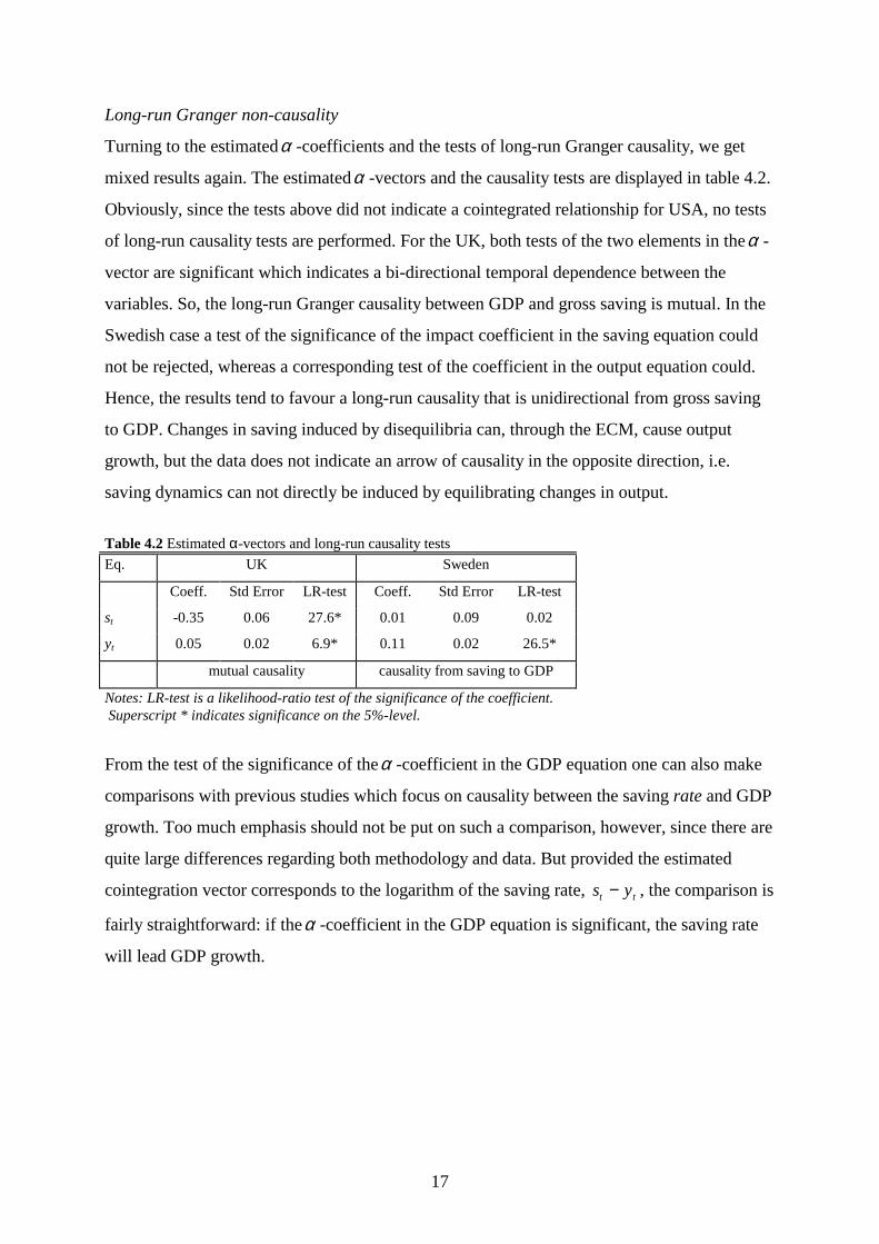
Turning to the estimatedα -coefficients and the tests of long-run Granger causality, we get

mixed results again. The estimatedα -vectors and the causality tests are displayed in table 4.2.

Obviously, since the tests above did not indicate a cointegrated relationship for USA, no tests

of long-run causality tests are performed. For the UK, both tests of the two elements in theα -

vector are significant which indicates a bi-directional temporal dependence between the

variables. So, the long-run Granger causality between GDP and gross saving is mutual. In the

Swedish case a test of the significance of the impact coefficient in the saving equation could

not be rejected, whereas a corresponding test of the coefficient in the output equation could.

Hence, the results tend to favour a long-run causality that is unidirectional from gross saving

to GDP. Changes in saving induced by disequilibria can, through the ECM, cause output

growth, but the data does not indicate an arrow of causality in the opposite direction, i.e.

saving dynamics can not directly be induced by equilibrating changes in output.

Table 4.2 Estimated α-vectors and long-run causality testsEq. UK Sweden

Coeff. Std Error LR-test Coeff. Std Error LR-test

st -0.35 0.06 27.6* 0.01 0.09 0.02

yt 0.05 0.02 6.9* 0.11 0.02 26.5*

mutual causality causality from saving to GDP

Notes: LR-test is a likelihood-ratio test of the significance of the coefficient. Superscript * indicates significance on the 5%-level.

From the test of the significance of theα -coefficient in the GDP equation one can also make

comparisons with previous studies which focus on causality between the saving rate and GDP

growth. Too much emphasis should not be put on such a comparison, however, since there are

quite large differences regarding both methodology and data. But provided the estimated

cointegration vector corresponds to the logarithm of the saving rate, s yt t− , the comparison is

fairly straightforward: if theα -coefficient in the GDP equation is significant, the saving rate

will lead GDP growth.

18

With another cointegrating vector a comparison is more far-fetched, and will have to be more

in terms of whether a long-run stationary relationship between output and saving will lead

output dynamics. Judging by the results from table 4.2 there is a temporal link from the

”saving rate” - for Sweden only modified to include a trend - to the growth rate, and in both

countries a higher saving rate precedes a higher growth rate. The fact that this link is positive

for both countries is at odds with some results in previous investigations (see section 2) but

allows a straight-forward interpretation that positive saving shocks disrupt the long-run

equilibrium upwards such that a higher growth rate is induced, at least temporarily.

Short-run Granger non-causality

Table 4.3 presents results from the VEC-regressions for the UK and Sweden, and the VAR-

regression in first-differences for the US. As it turns out, these causal chains are the only ones

that are statistically significant. The only fluctuations of output and saving which can be

explained by changes in the other variable in the system are changes stemming from error-

correction dynamics. Of course, this result is to some extent predetermined by the modelling

procedure. In the Swedish case for example, the specification search favoured a VAR(1),

which transforms into a VECM(0). Thus, short-run dynamics have already been rejected.

Table 4.3 Estimates from VAR/VEC regressionsRegressors USA UK Sweden

∆st ∆yt ∆st ∆yt ∆st ∆yt

constant 0.007

(0.012)

0.024*

(0.007)

-12.250*

(2.127)

1.695*

(0.744)

0.052

(0.141)

0.213*

(0.030)

ECMt-1 -0.320*

(0.056)

0.044*

(0.019)

0.013

(0.087)

0.115*

(0.019)

∆st-1 -0.302

(0.262)

-0.233

(0.142)

-0.166

(0.094)

-0.047

(0.033)

∆yt-1 0.764

(0.489)

0.391

(0.264)

0.257

(0.375)

0.433*

(0.131)

vec. Far5 0.43 1.42 0.94

vec. Fhet 0.77 0.49 0.45

vec. χ2norm 2.15 1.25 2.82

Notes: std errors in parenthesis. The order of the lag length is consistent with the preferred VAR-models foreach country, so that a VAR(p) is transformed to a VEC(p-1). ECM is the restricted estimated cointegratedrelationship. The last three tests are vector diagnostic tests of the residuals from the estimations: vec. Far5 is anF-test of up to 5th order residual vector serial correlation, vec. Fhet tests vector heteroscedasticity, and vec. χ2

normis a chi-square test of joint normality of the residuals. A * indicates significance on the 5%-level.

19

So, in neither of the three countries do the lagged first difference of saving have significant

explanatory power in the output equation and vice versa, at least using the traditional 5%

significance level. This does not necessarily mean a total absence of short-run causal chains

on the annual frequency. For both the US and the UK the lagged first-difference of saving do

have some explanatory power for output dynamics, and border on statistical significance on

the 10% level. This is also the case for lagged output growth in the saving equation in the US.

5 Discussion of results

There are two main results from the Granger non-causality tests above which have not

attracted much attention in previous studies. The first is that the Granger-causality between

saving and GDP is different across countries. For the UK and for Sweden, where standard

tests indicate a long-term relationship between the variables, the temporal interdependence

differs. In the UK, there is a bi-directional causality between GDP and gross saving in that

long-run equilibrating adjustments precede changes in both variables. In the Swedish case, the

temporal dependence is more unidirectional in its nature since saving dynamics can lead

output growth, but adjustments of output to correct a disequilibrium do not lead saving

dynamics. For the US there is no statistically significant long-run relationship between the

variables over the period studied here.

The second result is that the variables can be connected in Granger-causal chains through

different channels, in ‘long run‘ and ‘short run‘ chains, which might differ both regarding

direction and sign. As was emphasised above, the terminology is not to be taken in a temporal

sense but is meant to separate dynamics associated with adjustments to a long-run stationary

relationship from that of other stochastic shocks. Conditional on the presence of long-run

chains through the error-correction mechanism there are no statistically significant short-run

chains for Sweden. However, both for the US, where no long-run chain was found, and the

UK there are indications of short-run chains, even though they are not significant on

traditional significance levels; in the US the short-run causality runs in both directions while

the UK appears to have a unidirectional chain from saving to output.

20

Connecting back to the theoretical predictions in section 2 above, it is evident that the results

presented here are just as diverse as one would expect from that discussion. The fact that there

is a long-run stationary relation between gross saving and output for two of the countries

conforms to the most elementary of the predictions from growth theory. From the

cointegration tests it is clear that a variable close to the logarithm of the saving rate can be

considered a stationary variable for Sweden during this period, but not for the UK. The plot of

the saving rates for the countries in figure 4.1 may give some intuition for this result; the

Swedish saving rate appears to be fluctuating around a fairly constant level, while the

evolution of the saving rate in the UK is dominated by a positive trend during most of the

period.

One interpretation in terms of the Ramsey model presented in section 2 is that both results are

consistent with transitional dynamics toward steady states, but with different relations

between the underlying structural parameters in each country. In this context, the Swedish

transition path would correspond to the case where the saving rate is constant, or at least

randomly fluctuating around a certain level, implying a steady-state saving rate very close to

the intertemporal elasticity of substitution with the Cobb-Douglas parameterisation. The

evolution of the UK saving rate on the other hand would be more in line with a situation

where the steady-state saving rate is larger than the substitution elasticity, resulting in a

positively trended saving-rate transition path.

21

One possibility is that the steady-state saving rate is higher in the UK than in Sweden which

would make a trended transition path more likely for the UK. This explanation is supported by

the traditional arguments for differing saving rates across countries; the extension of the social

security system, the high female labour supply, and the high degree of ageing of the

population in Sweden, all point to a relatively lower Swedish saving rate. However, there

must be more to this story since the UK gross saving rate in fact has been below the Swedish

during the period, even during the first three decades when, except for the beginning of the

70s, the UK saving rate showed a clear positive trend. Another reason for the different

transitional patterns could be that UK households in the aggregate display a relatively lower

willingness to substitute consumption intertemporally. The same arguments that supported a

higher UK steady-state saving rate could be made to support this explanation. For example,

the female participation rate, which has been relatively higher in Sweden, has been found to

affect the intertemporal substitution elasticity positively (Blundell et al, 1994).

The fact that there is not much that points to a long-run relation between saving and output in

the US is harder to reconcile with traditional growth models.12 Intuitively, it is difficult to

combine a situation with no cointegration between saving and output with dynamics where the

variables follow stable transition paths. However, the plot of the saving rate for the US in

figure 4.1 might explain this result to some extent. Up to around 1980 the saving rate

fluctuated around a fairly stable level - perhaps with a slight negative trend. By 1980 there

was a very clear break in the series and from 1980 and on the saving rate dropped

dramatically. In view of the fact that unit root and cointegration tests are sensitive to trend

breaks, the inability to find a stationary relation between output and saving for the US should

not come as a complete surprise. Crude regressions using data up to the 1980s actually suggest

a stationary saving rate during the first three decades.

12 The specification used here might just be too simple, and detecting the true dynamics might be obscured by therather poor fit of the model. It is for example difficult to find a data congruent model of output and saving for theUS when the 1950s are included in regressions on quarterly data. Nonetheless, the fact that a joint model ofoutput and saving does not explain much of the dynamics of the two variables is an interesting result in itself.

22

Of course, the drop of the US saving rate, both on the national level and the household level,

in the 1980s has been the focus of numerous studies, but so far there has been no agreement

on one particular cause behind this phenomenon. This pronounced break naturally raises the

question of regime shifts, and a number of reasons for such a shift in the 1980s, e.g. financial

market developments, social security and health care extensions, changing demographic

structure, have been offered as explanations for the development of the US saving behaviour.

A deeper analysis of these matters has not been made here but could be taken into account

explicitly by estimation of Markov-switching VARs for example. This would, however, add

further complexity to the causality analysis since specific regimes and switches between

specific regimes might be associated with different causal relations.13

Admittedly, the discussion of the estimated cointegrated relations above is a rather intuitive

interpretation. The estimated model is not rigorously tied to any particular underlying theory.

Other interpretations of these results are of course possible.14 Still, even though the close

connection between saving and output is confirmed for two of the countries, the results also

show that the claim that saving is the driving force in this relationship clearly is too strong.

The notion may fit the Swedish results where the causality mainly runs from saving to output,

but it does not apply to the UK or US experience. For the UK deviations from the long-term

relationship will induce changes in both saving and output in order to re-establish the

equilibrium.

13 For an applied analysis of Granger-causality in MS-VARs see for example Jacobson, Lindh and Warne (1998)where focus is on saving, growth, and financial-market expansions in the US.14 As for example in the literature focused on testing neo-classical growth models with stochastic technologicalprogress (e.g. Neusser, 1991 - see discussion above).

23

Some clues to the propagation mechanisms behind these causal chains should be given by the

sign of the estimated coefficients. The long-run relation between saving and output is included

with a positive sign in the output equations for both UK and Sweden, so increases in saving

relative to output the previous period lead increases in output this period. This is consistent

with the ”mechanical” link through capital accumulation, i.e. the mechanism in focus of the

neo-classical growth models. Positive disequilibria, possibly resulting from higher saving, will

result in increased output. For the UK there is a mutual dependence where causality also runs

from output to saving. Since the error-correction mechanism is significant in the output

equation, positive adjustments to the ECM lead negative changes of gross saving. So,

increased output the previous period (relative to saving) will bring saving and output below

the stationary combination, which in turn will increase saving. Hence, relative increases in

output lead increased saving, a result that is in line with the traditional life-cycle model of

saving.

Even though the long-run causal chain is consistent with the mechanical capital accumulation

story behind growth, the short-run causality from saving to output for the UK and the US

shows the reversed sign; increases of saving precede output decreases. So here there is some

support for previous results that, to the extent that saving leads growth, it is with a negative

sign. A possible interpretation of this result is that of a traditional Keynesian aggregate-

demand effect; a positive shock to saving will reduce aggregate demand and therefore

temporarily dampen production increases.

Experiments with estimations of alternative specifications have been made to check the

robustness of the results above. These regressions have been of two types: estimations with a

pure investment variable and estimations with quarterly data instead of annual. Results from

these estimations are summarised in the appendix. On the whole, the results are consistent

across estimations with different variables, but differs somewhat depending on frequency of

the data. With annual data, there is a cointegrating combination of output and fixed

investment for the UK and Sweden which is close to the relationship for saving found above.

24

The long-run causal patterns between investment and GDP are also the same as for saving,

with the exception that UK error-correction dynamics is included in the investment equation

with a positive sign, indicating that increased output relative to investment will lead

investment decreases. However, as opposed to the case with gross saving, there are

statistically significant short-run causal chains, and for the UK there is a positive link from

output to investment via the short-run causal chain which is more in line with predictions

from accelerator-type models of investment. In the UK there is also a short-run link in the

other direction from investment to output, while Sweden has a unidirectional chain from

investment to output. The finding of no long-run relationship between a capital-accumulation

measure and output for the US is a surprisingly robust result. Virtually all experiments with

different variable definitions, dummy sets, and data frequencies fail to detect a cointegrating

relationship.

Results from estimations with quarterly data for the UK are similar for saving and investment,

but is somewhat different from the results with annual data; the cointegrating relationship

between output and saving/investment is similar, but the results from the long-run Granger

causality tests are not. The long-run causal chain in both cases is unidirectional from output to

gross saving or fixed investment, while the chain is bi-directional with annual data. This

suggests that the effect from saving/investment on output is a process that takes longer time to

be effective than the link in the other direction. There is a short-term link from saving to

output, but no statistically significant link in either direction for investment.

For Sweden the results with quarterly data are very different from the annual results; none of

the tests find evidence of a cointegrating relationship between saving/investment and output.

However, as mentioned above, the time span of the quarterly data for Sweden (1970:1 -

1998:3) is short and could be inadequate to detect long-run features. There is for example

some evidence from unit-root tests that both gross saving and fixed investment can be

considered I(0) series for this particular time period. Furthermore, since the quarterly data for

Sweden are seasonally unadjusted, dealing with integrated components of the seasonal

processes add additional considerations to the cointegration tests15.

15 More specifically, since seasonal unit roots might distort tests of cointegration between the non-seasonallyintegrated parts of the variables it is important to identify the seasonal processes. Here, tests of cointegration ”atthe zero frequency” between variables are made after seasonal differencing to remove any seasonal unit rootspresent according to HEGY-tests (Hylleberg et al, 1992). As it turns out seasonal roots might not be a problem,

25

In sum, the results confirm the findings in previous studies to some extent; there is more to the

saving/growth relationship than the ‘capital fundamentalist‘ view. On the other hand, a case

can be made for the argument that fluctuations of the saving rate, or another measure of the

long-run relationship between saving and output, precede positive growth. However, as

mentioned above, the point of the analysis here is that the causal chains are more complex

than this, and that the temporal dependence between output and gross saving will depend on

country characteristics and what type of dynamics one is studying.

Furthermore, focus really should not be on the saving rate - particularly if the purpose is to

interpret these causal chains in terms of policy recommendations. From a theoretical view the

relation between the saving rate and the growth rate is ambiguous, and from an empirical

view, since it is a combination of two non-stationary variables, the saving rate is at best a

long-run combination toward which output and saving tend to gravitate. To establish whether

incentives to increase saving really are growth promoting one should concentrate on

determining the causal chains linking total saving and output. As we have seen, there is indeed

evidence of such a positive link, but also of feed-back links.

Finally, from the estimations above it is clear that reliance on the mechanical link between

capital accumulation and growth as the major source of growth dynamics does not appear

promising; a large part of the changes in gross saving and GDP are left to explain when we

model these two variables bivariately. However, the goal here is not to explain saving or GDP

growth, but rather to investigate a temporal relationship between these variables. A more

realistic specification left for future research would include other potentially important

variables to test whether the information content of gross saving contained in GDP, and vice

versa, is stemming from a third underlying variable. The results from the exercise above

simply show the need for more careful theoretical and empirical modelling of the

determination of the saving rate and the dynamics of the saving/output relationship over time

and across countries, where country heterogeneity might be due to differences in demographic

structure, trade patterns, institutional or financial market features.

at least for fixed investment and output, since tests indicate different roots for these variables. The GDP seriesincludes an annual seasonal root, fixed investment a half-annual root, while the tests for gross saving indicateseasonal unit roots at all frequencies.

26

Appendix

Summary of results of cointegration tests and tests of long and short-run Granger non-causality with annual andquarterly data, and for gross saving and fixed investment.

USA UK Sweden

saving investment saving investment saving investment

Annual

ECM s y tt t− +4 0 07. i y tt t− +4 5 0 08. . s y tt t− −0 004. i y tt t− +2 0 03.

GC l-r s y+ →

s y+←

i y+ →

i y−←

s y+ → i y+ →

GC s-r s y?− →

s y?+←

s y?− → i y− →

i y+←

i y− →

Quart.

ECM s y tt t− +3 0 01. i y tt t− +35 0 01. .

GC l-r s y+← i y+←

GC s-r s y+ → i y+ → s y− → nc nc

Notes: the upper part of the table contains results from estimations with annual data, and the lower part resultswith quarterly data. ECM is the estimated restricted cointegrated relationship, GC l-r is the estimated long-runGranger causal chain between the variables, and GC s-r the estimated short-run chain. The sign above or belowthe ‘arrow of causality‘ indicates the sign of the causal chain. However, note the difficulty in interpreting thissign. The effect from saving on output, for example, refers to the effect from a positive deviation fromequilibrium, i.e. either a relative increase or relative decrease of saving compared to output. The effect fromoutput on saving, on the other hand, refers to a negative disequilibrium, i.e. either a relative increase or relativedecrease of output compared to saving. A blank field means that no statistically significant (on the 5%-level)relationship was found. The abbreviation nc means that a test was not calculated. Note the uncertainty(indicated by a ?) of some of the estimated relations for the US and the UK. These estimated short-run causalchains were not significant on traditional levels, but bordered on significance on the 10%-level. More detailedoutput of the estimations and tests are available on request.

27

References

Attanasio, O. (1997). ”Consumption and saving behaviour: modelling recent trends”. FiscalStudies. vol. 18, pp. 23-47.

Baltagi, B. H. (1995). Econometric Analysis of Panel Data. John Wiley & Sons. New York.

Barro, R. J., and Sala-i-Martin, X. (1995). Economic Growth. International Editions 1995.McGraw-Hill Inc. New York.

Bentzel, R. (1959). ”Några synpunkter på sparandets dynamik”. In Festskrift tillägnad HalvarSundberg. Uppsala Universitets Årsskrift 1959:9. Uppsala.

Blomström, M., Lipsey, R. E., and Zejan, M. (1996). ”Is fixed investment the key to economicgrowth?”. The Quarterly Journal of Economics. vol. 111, pp. 269-76.

Blundell, R., Browning, M., and Meghir, C. (1994). ”Consumer demand and the life-cycleallocation of household expenditures”. Review of Economic Studies. vol. 61, pp. 57-80.

Carroll, C. D., and Weil, D. N. (1994). ”Saving and growth: a reinterpretation”. Carnegie-Rochester Conference Series on Public Policy. vol. 40, pp. 133-192.

Campbell, J. Y. (1987). ”Does saving anticipate declining labor income? An alternative test ofthe permanent income hypothesis.” Econometrica. vol. 55, pp. 1249-1273.

Deaton, A. (1992). Understanding Consumption. Oxford University Press. Oxford.

Deaton, A. (1997). ”Saving and growth”. Working Paper. No 180. Research Program inDevelopment Studies. Princeton University.

Dolado, J. J., and Lütkepohl, H. (1996). ”Making Wald tests work for cointegrated VARsystems”. Econometric Reviews. vol. 15, pp. 369-386.

Doornik, J. A., and Hendry, D. F. (1997). Modelling Dynamic Systems Using PcFiml 9.0 forWindows. International Thomson Business Press. London.

Flavin, M. (1981). ”The adjustment of consumption to changing expectations about futureincome”. Journal of Political Economy. vol. 89, pp. 974-1009.

Granger, C. W. J. (1969). ”Investigating causal relations by econometric models and crossspectral methods”. Econometrica. vol. 37, pp. 424-438.

Granger, C. W. J. (1988). ”Some recent developments in a concept of causality”. Journal ofEconometrics. vol. 39, pp. 199-211.

Hakkio, C. S., and Rush, M. (1991). ”Cointegration: how short is the long run?”. Journal ofInternational Money and Finance. vol. 10, pp. 571-581.

28

Hylleberg, S. (ed). (1991). Modelling Seasonality. Oxford University Press. Oxford.

In, F., and Doucouliagos, C. (1997). ”Human capital formation and US economic growth: acausality analysis”. Applied Economics Letters. vol. 4, pp. 329-331.Jacobson, T., Lindh, T., and Warne, A. (1998). ”Growth, savings, financial markets andMarkov switching regimes”. Sveriges Riksbank Working Paper Series. No. 69.

Johansen, S. (1988). ”Statistical analysis of cointegration vectors”. Journal of EconomicDynamics and Control. vol. 12, pp. 231-254.

King, R. G., and Levine, R. (1994). ”Capital fundamentalism, economic development, andeconomic growth”. Carnegie-Rochester Conference Series on Public Policy. vol. 40, pp. 259-292.

King, R. G., Plosser, C. I., Stock, J. H., and Watson, M. W. (1991). ”Stochastic trends andeconomic fluctutations”. American Economic Review. vol. 81, pp. 819-840.

Lee, K., Pesaran, M. H., and Smith, R. (1997). ”Growth and convergence in a multi-countryempirical stochastic Solow model”. Journal of Applied Econometrics. vol. 12, pp. 357-392.

Levine, R., and Renelt, D. (1992). ”A sensitivity analysis of cross-country regressions”.American Economic Review. vol. 81, pp. 942-963.

Masih, R., and Masih, A. M. M. (1996). ”Macroeconomic activity dynamics and Grangercausality: new evidence from a small developing economy based on a vector error-correctionmodelling analysis”. Economic Modelling. vol. 13, pp. 407-426.

Modigliani, F. (1986). ”Life cycle, individual thrift, and the wealth of nations”. AmericanEconomic Review. vol. 76, pp. 297-313.

Modigliani, F., and Brumberg, R. (1954). ”Utility analysis and the consumption function: aninterpretation of cross-section data”. In K. Kurihara, (ed.). Post-Keynesian Economics.Rutgers University Press, New Brunswick.

Modigliani, F., and Brumberg, R. (1979). ”Utility analysis and the aggregate consumptionfunction: an attempt at integration”. In A. Abel, (ed.). Collected Papers of Franco Modigliani.Vol 2. MIT Press, Cambridge, Mass.

Mosconi, R., and Giannini, C. (1992). ”Non-causality in cointegrated systems: representationestimation and testing”. Oxford Bulletin of Economics and Statistics. vol. 54, pp. 399-417.

Neusser, K. (1991). ”Testing the long-run implications of the neoclassical growth model”.Journal of Monetary Economics. vol. 27, pp. 3-37.

Paxson, C. (1996). ”Saving and growth: evidence from micro data”. European EconomicReview. vol. 40, pp. 255-288.

Pesaran, M. H, and Smith, R. P. (1998). ”Structural analysis of cointegrating VARs”. DAEWorking Paper 9811. Department of Applied Economics. University of Cambridge.

29

Phillips, P. C. B. (1995). ”Fully modified least squares and vector autoregression”.Econometrica. vol. 63, pp. 1023-1078.

Rebelo, S. (1991). ”Long-run policy analysis and long-run growth”. Journal of PoliticalEconomy. vol. 99, pp. 500-521.

Sala-i-Martin, X. (1997). ”I just ran two million regressions”. American EconomicAssociation Papers and Proceedings. vol. 87, pp. 178-183.

Sims, C. (1972). ”Money, income, and causality”. American Economic Review. vol. 62, pp.540-552.

Sinha, D., and Sinha, T. (1998). ”Cart before the horse? The saving-growth nexus in Mexico”.Economics Letters. vol. 61, pp. 43-47.

Toda, H. Y., and Phillips, P. C. B. (1993). ”Vector autoregressions and causality”.Econometrica. vol. 61, pp. 1367-1393.

Toda, H. Y., and Phillips, P. C. B. (1994). ”Vector autoregressions and causality: a theoreticaloverview and simulation study”. Econometric Reviews. vol. 13, pp. 259-285.

Toda, H. Y., and Yamamoto, T. (1995). ”Statistical inference in vector autoregressions withpossibly integrated processes”. Journal of Econometrics. vol. 66, pp. 225-250.

Vanhoudt, P. (1998). ”A fallacy in causality research on growth and capital accumulation”.Economics Letters. vol. 60, pp. 77-81.

Zapata, H. O., and Rambaldi, A. N. (1997). ”Monte carlo evidence on cointegration andcausation”. Oxford Bulletin of Economics and Statistics. vol. 59, pp. 285-298.

Zellner, A. (1988). ”Causality and causal laws in economics”. Journal of Econometrics. vol.39, pp. 7-21.