On the Analysis of Public-Key Cryptologic Algorithms · Acknowledgements I would like to thank Arjen K. Lenstra for being a brilliant advisor. He gave me freedom to develop my ideas

POUR L'OBTENTION DU GRADE DE DOCTEUR ÈS SCIENCES

acceptée sur proposition du jury:

Prof. S. Vaudenay, président du juryProf. A. Lenstra, directeur de thèse

Dr J. W. Bos, rapporteur Dr P. C. Leyland, rapporteur

Prof. O. N. A. Svensson, rapporteur

On the Analysis of Public-Key Cryptologic Algorithms

THÈSE NO 6603 (2015)

ÉCOLE POLYTECHNIQUE FÉDÉRALE DE LAUSANNE

PRÉSENTÉE LE 7 MAI 2015

À LA FACULTÉ INFORMATIQUE ET COMMUNICATIONSLABORATOIRE DE CRYPTOLOGIE ALGORITHMIQUE

PROGRAMME DOCTORAL EN INFORMATIQUE ET COMMUNICATIONS

Suisse2015

PAR

Andrea MIELE

Alla mia famglia. . .

AcknowledgementsI would like to thank Arjen K. Lenstra for being a brilliant advisor. He gave me freedom to develop my

ideas and at the same time he constantly provided me with decisive advice. Being a part of LACAL

under his supervision made my research skills greatly improve.

I would like to thank present and former post-doctoral researchers from LACAL for their invaluable

help: Anja A. Becker, Robert Granger, Dimitar P. Jetchev, Marcelo E. Kaihara and Thorsten Kleinjung. A

special mention goes to Thorsten for continuously giving me useful feedback throughout all these years.

I would like to thank former and current PhD students from LACAL: Maxime Augier, Joppe W. Bos, Alina

Dudeanu, Seyyd Hasan Mirjalili, Onur Özen, Juraj Šarinay and Benjamin Wesolowski. Sharing thoughts

and ideas with you was great. Special thanks to Joppe for being an awesome work companion. Also, a big

thanks to our secretary Monique Amhof for her relentless help with administrative business. I am glad

I also had numerous chances to have fun with all of you outside of work, starting with our traditional

“movie-lunches”. Finally, I would like to thank Germana and my family for their unconditional and fair

support.

i

AbstractThe RSA cryptosystem introduced in 1977 by Ron Rivest, Adi Shamir and Len Adleman is the most

commonly deployed public-key cryptosystem. Elliptic curve cryptography (ECC) introduced in the mid

80’s by Neal Koblitz and Victor Miller is becoming an increasingly popular alternative to RSA offering

competitive performance due the use of smaller key sizes. Most recently hyperelliptic curve cryptogra-

phy (HECC) has been demonstrated to have comparable and in some cases better performance than

ECC. The security of RSA relies on the integer factorization problem whereas the security of (H)ECC is

based on the (hyper)elliptic curve discrete logarithm problem ((H)ECDLP). In this thesis the practical

performance of the best methods to solve these problems is analyzed and a method to generate secure

ephemeral ECC parameters is presented.

The best publicly known algorithm to solve the integer factorization problem is the number field

sieve (NFS). Its most time consuming step is the relation collection step. We investigate the use of

graphics processing units (GPUs) as accelerators for this step. In this context, methods to efficiently

implement modular arithmetic and several factoring algorithms on GPUs are presented and their

performance is analyzed in practice. In conclusion, it is shown that integrating state-of-the-art NFS

software packages with our GPU software can lead to a speed-up of 50%.

In the case of elliptic and hyperelliptic curves for cryptographic use, the best published method

to solve the (H)ECDLP is the Pollard rho algorithm. This method can be made faster using classes of

equivalence induced by curve automorphisms like the negation map. We present a practical analysis of

their use to speed up Pollard rho for elliptic curves and genus 2 hyperelliptic curves defined over prime

fields. As a case study, 4 curves at the 128-bit theoretical security level are analyzed in our software

framework for Pollard rho to estimate their practical security level.

In addition, we present a novel many-core architecture to solve the ECDLP using the Pollard rho

algorithm with the negation map on FPGAs. This architecture is used to estimate the cost of solving the

Certicom ECCp-131 challenge with a cluster of FPGAs. Our design achieves a speed-up factor of about

4 compared to the state-of-the-art.

Finally, we present an efficient method to generate unique, secure and unpredictable ephemeral

ECC parameters to be shared by a pair of authenticated users for a single communication. It provides

an alternative to the customary use of fixed ECC parameters obtained from publicly available standards

designed by untrusted third parties. The effectiveness of our method is demonstrated with a portable

implementation for regular PCs and Android smartphones. On a Samsung Galaxy S4 smartphone our

implementation generates unique 128-bit secure ECC parameters in 50 milliseconds on average.

Key words: cryptology, cryptanalysis, public-key cryptography, integer factorization, elliptic curves,

hyperelliptic curves, discrete logarithm problem, GPUs, FPGAs, complex multiplication method

iii

ZusammenfassungDas 1977 von Ron Rivest, Adi Shamir und Len Adleman entwickelte RSA Kryptosystem ist heutzutage

das am häufigsten verwendete. Mitte der 80er Jahre wurde die Elliptische-Kurven-Kryptographie

(ECC) entwickelt, die wegen ihrer vergleichsweise guten Leistung eine immer beliebtere Alternative

zu RSA geworden ist. Vor kurzem wurde gezeigt, dass Hyperelliptische-Kurven-Kryptographie (HECC)

vergleichbare und in einigen Fällen sogar bessere Leistung im Vergleich zu ECC bietet. Die Sicherheit

von RSA basiert auf dem Faktorisierungsproblem, wohingegen die Sicherheit von (H)ECC auf dem

Problem des diskreten Logarithmus für (hyper)elliptische Kurven ((H)ECDLP) beruht. In dieser Arbeit

werden die besten Methoden zur Lösung solcher Probleme auf ihre praktische Verwendbarkeit hin

untersucht. Ausserdem wird eine Methode zur Erzeugung von flüchtigen ECC Parametern vorgestellt.

Der beste bekannte Algorithmus zur Lösung des Faktorisierungsproblems für ganze Zahlen ist das

Zahlkörpersieb (NFS), dessen zeitintensivster Schritt das Suchen von Relationen ist. Wir untersuchen,

inwieweit Grafikprozessoren (GPUs) diesen Schritt beschleunigen können. Dafür werden Methoden

zur effizienten GPU-Implementierung von modularer Arithmetik sowie von diversen Faktorisierungsal-

gorithmen vorgestellt, und ihre Leistung wird analysiert. Ausserdem wird gezeigt, dass die Integration

unserer GPU-Software in ein aktuelles NFS-Softwarepaket einen Geschwindigkeitszuwachs von 50%

ergeben kann.

Zur Lösung von (H)ECDLP ist die beste bekannte Methode Pollards rho Algorithmus. Durch die

Verwendung von Äquivalenzklassen, die durch Automorphismen der Kurve induziert werden (wie

beispielsweise die Negationsabbildung), lässt sich diese Methode beschleunigen. Obwohl die Verwen-

dung der Negationsabbildung schon umfangreich untersucht wurde, ist den anderen Automorphismen

bisher wenig Aufmerksamkeit zuteil geworden. Inwieweit sich Pollard rho mit diesen Automorphismen

beschleunigen lässt, untersuchen wir sowohl für elliptische Kurven als auch für hyperelliptische Kurven

vom Geschlecht 2. Als Fallbeispiel analysieren wir 4 Kurven des 128-Bit Sicherheitsniveaus, um ihr

genaues Sicherheitsniveau zu bestimmen.

Zusätzlich stellen wir eine neuartige FPGA-Architektur zum Lösen von ECDLP durch Pollard rho mit

Negationsabbildung vor. Damit können die Kosten eines FPGA-Verbundes zum Lösen von Certicoms

ECCp-131 Herausforderung abgeschätzt werden. Sie sind um einen Faktor 4 niedriger als die der besten

bekannten Implementierung.

Zum Schluss präsentieren wir eine effiziente Methode, um eindeutige, sichere und unvorhersagbare

flüchtige ECC Parameter für eine einzige Kommunikation zwischen zwei authentifizierten Partnern

zu erzeugen. Dies stellt eine Alternative zu der gebräuchlichen Praxis von festen ECC Parametern aus

öffentlichen, von nicht vertrauenswürdigen Dritten erstellten Standards dar. Die Effektivität unserer

Methode wird durch eine portable Implementierung für PCs und Android Smartphones demonstriert.

Auf einem Samsung Galaxy S4 Smartphone erzeugt sie im Durchschnitt alle 50 Millisekunden einen

Satz eindeutiger ECC Parameter im 128-Bit Sicherheitsniveau.

Stichwörter: Kryptologie, Kryptoanalyse, Kryptographie mit öffentlichen Schlüsseln, Faktorisierung

ganzer Zahlen, elliptische Kurven, hyperelliptische Kurven, Problem des diskreten Logarithmus, GPUs,

v

Zusammenfassung

FPGAs, Methode der komplexen Multiplikation

vi

RésuméLe système de cryptage RSA introduit en 1977 par Ron Rivest, Adi Shamir et Len Adleman est le

système cryptographique à clé publique le plus souvent déployé. La cryptographie sur les courbes

elliptiques, ou ECC, introduite dans le milieu des années 80 par Neal Koblitz et Victor Miller devient

une alternative de plus en plus populaire pour RSA grâce à ses performances compétitives en raison

de l’utilisation de tailles de clés plus courtes. Plus récemment il a été démontré que la cryptographie

sur les courbes hyperelliptiques ou HECC offre des performances comparables et, dans certains cas,

meilleures que ECC. La sécurité de RSA repose sur le problème de factorisation d’entiers tandis que la

sécurité de (H)ECC est basée sur le problème du logarithme discret dans le groupe correspondant à la

courbe (hyper)elliptique, abrégé (H)ECDLP. Dans cette thèse les performances pratiques des meilleures

méthodes pour résoudre ces problèmes sur différentes plates-formes sont analysées et une méthode

pour générer des paramètres éphémères sécurisés pour ECC est étudié.

Le meilleur algorithme publiquement connu pour résoudre le problème de factorisation d’entiers

est le crible sur les corps de nombres, ou NFS. L’étape de NFS qui prend le plus de temps est l’étape de

collection de relations. Nous étudions l’utilisation de cartes graphiques ou GPU comme accélérateurs

pour cette étape. Dans ce contexte, des méthodes pour implémenter efficacement l’arithmétique

modulaire et plusieurs algorithmes de factorisation sur GPU sont présentées et les leurs performances

pratiques sont analysées. En conclusion, il est démontré que l’intégration des implémentations à l’état

de l’art de NFS pour CPU avec notre logiciel pour GPU peut conduire à une acc’el’eration de 50%.

Dans le case de courbes elliptiques et hyperelliptiques pour l’utilisation cryptographique la mé-

thode la plus rapide connue pour résoudre l’(H)ECDLP est l’algorithme du Rho de Pollard. Cette

méthode peut àtre accélérée en utilisant des classes d’équivalence induite par automorphismes d’une

courbe comme la négation. Nous présentons une analyse pratique de leur utilisation pour accélérer

l’algorithme du Rho de Pollard sur les courbes elliptiques et courbes hyperelliptiques de genre 2 et

nous analysons 4 courbes au niveau de sécurité théorique de 128 bit dans notre cadre logiciel pour

Pollard Rho pour estimer leur niveau de sécurité pratique.

En outre, nous présentons une nouvelle architecture multi-coeurs pour résoudre l’ECDLP en

utilisant l’algorithme du Rho de Pollard avec la négation sur FPGA. Cette architecture est utilisée pour

estimer le coût de résoudre le défi Certicom ECCp-131 avec un groupe de FPGA. Notre architecture

permet d’atteindre un facteur d’accélération de approximativement 4 par rapport à l’état de l’art.

Enfin, nous présentons une méthode efficace pour générer des paramètres éphémères uniques,

sécurisés et imprévisibles pour ECC destinés à être partagé par une paire d’utilisateurs authentifiés

pour une seule communication. Il offre une alternative à l’utilisation coutumière de paramètres pour

ECC fixés par des normes publiques conçues par des tiers non fiables. L’efficacité de notre méthode

est démontrée avec une implémentation portable pour PC et pour smartphones avec Android. Sur un

smartphone Samsung Galaxy S4 notre implémentation génère des paramètres uniques sécurisés à 128

bit de sécurité pour ECC en 50 millisecondes en moyenne.

Mots clefs : cryptologie, cryptanalyse, cryptographie à clé publique, factorisation d’entiers, courbes

vii

Résumé

elliptiques, courbes hyperelliptiques, problème du logarithme discret, GPU, FPGA, méthode de la

multiplication complexe

viii

SommarioL’algoritmo RSA introdotto nel 1977 da Ron Rivest, Adi Shamir et Len Adleman è il sistema di crittografia

a chiave pubblica maggiormente utilizzato. La crittografia basata su curve ellittiche, o ECC, introdotta

alla metà degli anni 80 da Neal Koblitz e Victor Miller sta diventando un’alternativa all’RSA sempre

più popolare grazie alle sue prestazioni competitive dovute all’utilizzo di chiavi di dimensione minore.

Recentemente è stato dimostrato che la crittografia basata su curve iperellittiche, o HECC, fornisce

prestazioni simili e in alcuni casi superiori ad ECC. In questa tesi la sicurezza dell’RSA è basata sul

problema della fattorizzazione di numeri interi mentre la sicurezza di (H)ECC è basata sul problema

del logaritmo discreto su curve (iper)ellittiche, o abbreviato (H)ECDLP. In questa tesi sono analizzate

le prestazioni dei migliori metodi per la risoluzione di questi problemi su diverse piattaforme ed è

proposto un metodo per generare parametri sicuri “monouso” per ECC.

Il miglior algoritmo per risolvere il problema della fattorizzazione di numeri interi è il crivello di

campi numeri, o NFS. La fase dell’NFS che richiede più tempo è la “collezione di relazioni”. È presentata

l’analisi dell’uso di schede grafiche o GPU come acceleratori per questa fase dell’algoritmo. In questo

contesto sono descritti metodi per l’implementazione efficiente dell’aritmetica modulare e di diversi

algoritmi di fattorizzazione di numeri interi su GPU e ne sono analizzate le prestazioni nella pratica.

In conclusione, è dimostrato che l’integrazione del nostro software per GPU con implementazioni

dell’NFS allo stato dell’arte risulta in uno speed-up fino al 50%.

Se si considerano curve ellittiche e iperellittiche per uso crittografico, Il miglior metodo per la riso-

luzione dell’(H)ECDLP è il metodo rho di Pollard. Questo metodo può essere accelerato utilizzando le

classi di equivalenza indotte dagli automorfismi delle curve come la mappa di negazione. È presentata

un’analisi pratica dell’uso di questi automorfismi per accelerare il metodo rho di Pollard sia nel caso

delle curve ellittiche che in quello delle curve iperellittiche e quattro curve al livello teorico di sicurezza

di 128 bit sono analizzate all’interno del nostro framework software per il metodo rho di Pollard al fine

di stimare il loro livello di sicurezza pratico.

È inoltre presentata un’architettura many-core innovativa per la risoluzione dell’ECDLP su FPGA

che implementa il metodo rho di Pollard con la mappa di negazione. Questa architettura è utilizzata

per stimate il costo monetario necessario per risolvere la challenge ECCp-131 pubblicata da Certicom

su un cluster di FPGA. Confrontata con lo stato dell’arte la nostra architettura ha prestazioni superiori

di circa 4 volte.

Infine, è presentato un metodo per generare parametri ECC monouso unici, sicuri e non predi-

cibili per l’utilizzo in un’unica sessione da parte di due utenti autenticati. Questo metodo fornisce

un’alternativa all’uso classico di parametri ECC fissi forniti da standard pubblici prodotti da terze parti

(non necessariamente affidabili). L’efficienza del nostro metodo è dimostrata con un’implementazione

portabile per PC e smartphone equipaggiati con il sistema operativo Android. Su un Samsung Galaxy

S4 il nostro software impiega in media 50 millisecondi per generare parametri ECC unici al livello di

sicurezza di 128 bit.

Parole chiave: crittologia, crittanalisi, crittografia a chiave pubblica, fattorizzazione di numeri

ix

Sommario

interi, curve ellittiche, curve iperellittiche, problema del logaritmo discreto, GPU, FPGA, metodo della

moltiplicazione complessa

x

ContentsAcknowledgements i

Abstract (English/Deutsch/Français/Italian) iii

List of figures xiii

List of tables xv

1 Introduction 1

2 Background 5

2.1 Large integer representation . . . . . . . . . . . . . . . . . . . . . . . . . . . . . . . . . . . . 5

2.2 Smooth positive integers . . . . . . . . . . . . . . . . . . . . . . . . . . . . . . . . . . . . . . . 5

2.3 L-notation . . . . . . . . . . . . . . . . . . . . . . . . . . . . . . . . . . . . . . . . . . . . . . . 5

2.4 Arithmetic . . . . . . . . . . . . . . . . . . . . . . . . . . . . . . . . . . . . . . . . . . . . . . . 5

2.4.1 Montgomery arithmetic . . . . . . . . . . . . . . . . . . . . . . . . . . . . . . . . . . . 6

2.4.2 Exact division . . . . . . . . . . . . . . . . . . . . . . . . . . . . . . . . . . . . . . . . . 8

2.4.3 A divisibility test . . . . . . . . . . . . . . . . . . . . . . . . . . . . . . . . . . . . . . . 8

2.4.4 A compositeness test: Miller-Rabin . . . . . . . . . . . . . . . . . . . . . . . . . . . . 9

2.5 Elliptic curves and genus 2 hyperelliptic curves . . . . . . . . . . . . . . . . . . . . . . . . . 11

2.5.1 Weierstrass curves . . . . . . . . . . . . . . . . . . . . . . . . . . . . . . . . . . . . . . 11

2.5.2 Montgomery curves . . . . . . . . . . . . . . . . . . . . . . . . . . . . . . . . . . . . . 12

2.5.3 Edwards curves . . . . . . . . . . . . . . . . . . . . . . . . . . . . . . . . . . . . . . . . 13

2.5.4 Genus 2 hyperelliptic curves . . . . . . . . . . . . . . . . . . . . . . . . . . . . . . . . 14

2.6 Integer factorization algorithms . . . . . . . . . . . . . . . . . . . . . . . . . . . . . . . . . . 15

2.6.1 Trial division . . . . . . . . . . . . . . . . . . . . . . . . . . . . . . . . . . . . . . . . . . 16

2.6.2 Pollard p −1 . . . . . . . . . . . . . . . . . . . . . . . . . . . . . . . . . . . . . . . . . . 16

2.6.3 ECM . . . . . . . . . . . . . . . . . . . . . . . . . . . . . . . . . . . . . . . . . . . . . . 18

2.6.4 The number field sieve (NFS) . . . . . . . . . . . . . . . . . . . . . . . . . . . . . . . . 20

2.7 The Pollard rho algorithm for discrete logarithms . . . . . . . . . . . . . . . . . . . . . . . . 22

2.7.1 The Pollard rho algorithm for ECDLP . . . . . . . . . . . . . . . . . . . . . . . . . . . 22

2.7.2 Parallel Pollard rho . . . . . . . . . . . . . . . . . . . . . . . . . . . . . . . . . . . . . . 24

2.7.3 Using automorphisms to speed up Pollard rho . . . . . . . . . . . . . . . . . . . . . . 25

2.7.4 Detecting and escaping Fruitless Cycles . . . . . . . . . . . . . . . . . . . . . . . . . . 26

2.7.5 Handling automorphisms in practice . . . . . . . . . . . . . . . . . . . . . . . . . . . 27

2.8 Compute Unified Device Architecture (CUDA) . . . . . . . . . . . . . . . . . . . . . . . . . . 27

2.9 FPGAs . . . . . . . . . . . . . . . . . . . . . . . . . . . . . . . . . . . . . . . . . . . . . . . . . . 29

xi

Contents

3 Cofactorization on GPUs 333.1 Preliminaries . . . . . . . . . . . . . . . . . . . . . . . . . . . . . . . . . . . . . . . . . . . . . 34

3.2 Cofactoring Steps . . . . . . . . . . . . . . . . . . . . . . . . . . . . . . . . . . . . . . . . . . . 34

3.3 GPU Implementation Details . . . . . . . . . . . . . . . . . . . . . . . . . . . . . . . . . . . . 36

3.3.1 Compute unified device architecture . . . . . . . . . . . . . . . . . . . . . . . . . . . 36

3.3.2 Modular arithmetic on GPUs . . . . . . . . . . . . . . . . . . . . . . . . . . . . . . . . 36

3.3.3 Elliptic curve arithmetic on GPUs . . . . . . . . . . . . . . . . . . . . . . . . . . . . . 39

3.4 Cofactorization on GPUs . . . . . . . . . . . . . . . . . . . . . . . . . . . . . . . . . . . . . . . 40

3.4.1 Cofactorization overview . . . . . . . . . . . . . . . . . . . . . . . . . . . . . . . . . . 40

3.4.2 Parameter selection . . . . . . . . . . . . . . . . . . . . . . . . . . . . . . . . . . . . . 42

3.4.3 Performance results . . . . . . . . . . . . . . . . . . . . . . . . . . . . . . . . . . . . . 44

3.5 Conclusion . . . . . . . . . . . . . . . . . . . . . . . . . . . . . . . . . . . . . . . . . . . . . . . 44

4 Elliptic and Hyperelliptic Curves: a Practical Security Analysis 474.1 Preliminaries . . . . . . . . . . . . . . . . . . . . . . . . . . . . . . . . . . . . . . . . . . . . . 48

4.1.1 Handling Fruitless Cycles in Practice . . . . . . . . . . . . . . . . . . . . . . . . . . . 49

4.2 Target Curves and their Automorphism Groups . . . . . . . . . . . . . . . . . . . . . . . . . 50

4.2.1 Target Curves in Genus 1 . . . . . . . . . . . . . . . . . . . . . . . . . . . . . . . . . . 51

4.2.2 Target Curves in Genus 2 . . . . . . . . . . . . . . . . . . . . . . . . . . . . . . . . . . 52

4.2.3 Other Curves of Interest . . . . . . . . . . . . . . . . . . . . . . . . . . . . . . . . . . . 53

4.3 Performance Results . . . . . . . . . . . . . . . . . . . . . . . . . . . . . . . . . . . . . . . . . 54

4.3.1 Correctness . . . . . . . . . . . . . . . . . . . . . . . . . . . . . . . . . . . . . . . . . . 54

4.3.2 Implementation Results . . . . . . . . . . . . . . . . . . . . . . . . . . . . . . . . . . . 56

4.4 Conclusion . . . . . . . . . . . . . . . . . . . . . . . . . . . . . . . . . . . . . . . . . . . . . . . 57

5 An Efficient Many-Core Architecture for ECC security assessment 595.1 Parallel Pollard rho for the ECDLP on FPGAs . . . . . . . . . . . . . . . . . . . . . . . . . . . 59

5.2 Proposed architecture . . . . . . . . . . . . . . . . . . . . . . . . . . . . . . . . . . . . . . . . 60

5.2.1 Prime field operations . . . . . . . . . . . . . . . . . . . . . . . . . . . . . . . . . . . . 60

5.2.2 Single pipeline multi walk core . . . . . . . . . . . . . . . . . . . . . . . . . . . . . . . 62

5.2.3 Pipeline unrolling . . . . . . . . . . . . . . . . . . . . . . . . . . . . . . . . . . . . . . . 66

5.2.4 System level architecture . . . . . . . . . . . . . . . . . . . . . . . . . . . . . . . . . . 70

5.3 Experimental results . . . . . . . . . . . . . . . . . . . . . . . . . . . . . . . . . . . . . . . . . 71

5.4 Conclusion and future work . . . . . . . . . . . . . . . . . . . . . . . . . . . . . . . . . . . . . 73

6 Efficient ephemeral elliptic curve cryptographic keys 756.1 Preliminaries . . . . . . . . . . . . . . . . . . . . . . . . . . . . . . . . . . . . . . . . . . . . . 76

6.2 Special cases of the complex multiplication method . . . . . . . . . . . . . . . . . . . . . . 80

6.2.1 The CM method . . . . . . . . . . . . . . . . . . . . . . . . . . . . . . . . . . . . . . . . 80

6.2.2 The CM method for class numbers at most three . . . . . . . . . . . . . . . . . . . . 81

6.2.3 The CM method for larger class numbers . . . . . . . . . . . . . . . . . . . . . . . . . 82

6.3 Ephemeral ECC parameter generation . . . . . . . . . . . . . . . . . . . . . . . . . . . . . . 84

6.4 Security criteria . . . . . . . . . . . . . . . . . . . . . . . . . . . . . . . . . . . . . . . . . . . . 87

6.5 Conclusion and future work . . . . . . . . . . . . . . . . . . . . . . . . . . . . . . . . . . . . . 91

Bibliography 105

Curriculum Vitae 107

xii

List of Figures2.1 Pictorial view of a Pollard rho walk. . . . . . . . . . . . . . . . . . . . . . . . . . . . . . . . . 23

2.2 A distinguished point collision in parallel Pollard rho. . . . . . . . . . . . . . . . . . . . . . 25

2.3 High-level overview of a CUDA GPU architecture. . . . . . . . . . . . . . . . . . . . . . . . . 28

2.4 Memory coalescing in CUDA. . . . . . . . . . . . . . . . . . . . . . . . . . . . . . . . . . . . . 29

2.5 Generic FPGA architecture [175]. . . . . . . . . . . . . . . . . . . . . . . . . . . . . . . . . . . 30

2.6 Configurable logic block architecture. [207]. . . . . . . . . . . . . . . . . . . . . . . . . . . . 30

3.1 An example of kernel execution flow where the values are assumed to be at most 160

bits. The height of the dashed rectangles is proportional to the number of values that are

processed at a given step. . . . . . . . . . . . . . . . . . . . . . . . . . . . . . . . . . . . . . . 41

3.2 Rational kernel cofactoring run times as a function of the Pollard p − 1 bounds with

desired yield 95%. . . . . . . . . . . . . . . . . . . . . . . . . . . . . . . . . . . . . . . . . . . 43

5.1 Montgomery multiplication module. . . . . . . . . . . . . . . . . . . . . . . . . . . . . . . . 62

5.2 Inversion module. . . . . . . . . . . . . . . . . . . . . . . . . . . . . . . . . . . . . . . . . . . . 64

5.3 High-level view of the SPMW core. . . . . . . . . . . . . . . . . . . . . . . . . . . . . . . . . . 64

5.4 Single-Pipe Multi-Walks approach. . . . . . . . . . . . . . . . . . . . . . . . . . . . . . . . . . 65

5.5 Inversion module with state pre-loading. . . . . . . . . . . . . . . . . . . . . . . . . . . . . . 68

5.6 Replicated inversion module. . . . . . . . . . . . . . . . . . . . . . . . . . . . . . . . . . . . . 69

5.7 Unrolled pipeline with T P = 1/(dk/2e+1). . . . . . . . . . . . . . . . . . . . . . . . . . . . . 69

5.8 Montgomery multiplier with state pre-loading. . . . . . . . . . . . . . . . . . . . . . . . . . 70

5.9 System level architecture. . . . . . . . . . . . . . . . . . . . . . . . . . . . . . . . . . . . . . . 71

xiii

List of Tables2.1 Addition and doubling in the Jacobian group of a hyperelliptic curve C defined over an

odd characteristic field K in Mumford affine coordinates. . . . . . . . . . . . . . . . . . . . 15

2.2 NVIDIA GPU comparison: Fermi, Kepler and Kepler Titan. . . . . . . . . . . . . . . . . . . 28

3.1 Pseudo-code notation for CUDA PTX assembly instructions [162] used in our implemen-

tation. Function parameters are 32-bit unsigned integers and the suffixes are analogous to

the actual CUDA PTX suffixes. We denote by f the single-bit carry flag set by instructions

with suffix “.cc”. . . . . . . . . . . . . . . . . . . . . . . . . . . . . . . . . . . . . . . . . . . . . 37

3.2 Benchmark results for the NVIDIA GTX 580 GPU for number of Montgomery multiplica-

tions per second and ECM trials per second for various modulus sizes. The Montgomery

multiplication throughput reported in [123] was scaled as explained in the text. The

estimated peak throughput based on an instruction count is also included together with

the total number of dispatched threads. ECM used bounds B1 = 256 and B2 = 16384 (for

a total of 2844+3368 = 6212 Montgomery multiplications per trial). . . . . . . . . . . . . . 39

3.3 Time in seconds to process a single special prime on all cores of a quad-core Intel i7-3770K

CPU. . . . . . . . . . . . . . . . . . . . . . . . . . . . . . . . . . . . . . . . . . . . . . . . . . . 42

3.4 Parameters choices for cofactoring. Later ECM attempts use larger bounds in the specified

ranges. . . . . . . . . . . . . . . . . . . . . . . . . . . . . . . . . . . . . . . . . . . . . . . . . . 42

3.5 Approximate timings in seconds of cofactoring steps to process approximately 50 mil-

lion (a,b) pairs, measured using the CUDA clock64 instruction. The wall clock time

(measured with the unix time utility) includes the kernel launch overhead the CPU/GPU

memory transfer and all CPU book-keeping operations. . . . . . . . . . . . . . . . . . . . . 43

3.6 GPU cofactoring for a single special prime. The number of quad-core CPUs that can be

served by a single GPU is given in the second to last column. . . . . . . . . . . . . . . . . . 44

3.7 Processing multiple special primes with desired yield 99%. . . . . . . . . . . . . . . . . . . 45

4.1 Cost of the Pollard rho iteration for the selected genus g curves, where m = #Aut and q is

the prime field characteristic. We denote modular multiplications, modular squarings

and modular additions/subtractions with m, s and a respectively. When updating the ai

and bi values, we compute modulo the appropriate n instead of modulo q . . . . . . . . . 53

4.2 Summary of the number of steps required when solving the DLP in a prime order sub-

group n (2N−1 < n < 2N ) on the four (modified) curves we consider in this work. We

computed 10 batches of 103 discrete logarithms and we display the minimum and maxi-

mum number of average steps out of these 10 batches, as well as the overall average. We

used a 32-adding walk and a distinguished point property with d = 8, which we expect to

occur once every 28 steps. The expected estimate is derived using Eq. (4.4). . . . . . . . . 55

xv

List of Tables

4.3 A comparison of the expected (exp.) and real number of fruitless steps (FS) and fruitful

steps when computing 10 batches of 103 discrete logarithms (as in Table 4.2) but using

the group automorphism optimization. The genus-g curves have m = #Aut(C ) and we

check for cycles up to length β every α steps. . . . . . . . . . . . . . . . . . . . . . . . . . . . 56

4.4 The performance of our implementations expressed in the number of cycles per step with-

out (32-adding walk) and with (1024-adding walk) the usage of the group automorphism

running 2048 walks concurrently. For each curve, the expected speedup (which takes into

account the additional cost of computing the equivalence class representative) and the

speedup found in practice are stated together with the expected number of single-core

years to solve a discrete logarithm. The security of each curve is given when taking NIST

CurveP-256 as the baseline for the 128-bit security level. . . . . . . . . . . . . . . . . . . . . 57

5.1 Latencies of the modules composing the pipeline. . . . . . . . . . . . . . . . . . . . . . . . 66

5.2 Optimization parameters for Virtex-7-xc7v2000t FPGAs. Area figures are in number of slices. 71

5.3 Solving ECCp-131 in one year on (a cluster of) different FPGAs. Number of points to

compute: ≈√qπ/4. . . . . . . . . . . . . . . . . . . . . . . . . . . . . . . . . . . . . . . . . . 72

5.4 Comparison with [106] on a single Xilinx Virtex-5 vsx240t. . . . . . . . . . . . . . . . . . . . . . . 73

5.5 Comparison with [90] on a single Xilinx Spartan-3 xc3s5000. . . . . . . . . . . . . . . . . . . . . . 73

6.1 Timings of random cryptographic parameter generation using MAGMA on a single 2.7GHz

Intel Core i7-3820QM, averaged over 100 parameter sets, for prime elliptic curve group

orders and 80-bit, 112-bit, and 128-bit security. For RSA these security levels correspond,

roughly but close enough, to 1024-bit, 2048-bit, and 3072-bit composite moduli, for DSA

to 1024-bit, 2048-bit, and 3072-bit prime fields with 160-bit, 224-bit, and 256-bit prime

order subgroups of the multiplicative group, respectively. . . . . . . . . . . . . . . . . . . . 77

6.2 Elliptic curves for fast ECC parameter selection. Each row contains a value d , the class

number h−d of the imaginary quadratic field Q(p−d) with discriminant −d , the root

used (commonly referred to as the j -invariant), the elliptic curve E = Ea,b , the constraints

on the prime p and the values u and v , the value s such that #E (Fp ) = p +1− su, and with

γ and γ denoting fixed factors of #E(Fp ) and #E(Fp ), respectively. . . . . . . . . . . . . . . 83

6.3 Polynomial representation of p = p(X ), #E(Fp ) = ord(X ) and #E(Fp ) = ord(X ) for the

discriminants in Table 6.2. . . . . . . . . . . . . . . . . . . . . . . . . . . . . . . . . . . . . . . 86

6.4 Performance results in milliseconds for parameter generation at the 128-bit security level,

with `, ˜, f , P , and I as above, the “MF”-column to indicate Montgomery friendliness,

and µ the average and σ the standard deviation. . . . . . . . . . . . . . . . . . . . . . . . . . 87

6.5 Summary of performance results in milliseconds for parameter generation at different

security levels: 80-bit, 112-bit, 128-bit, 160-bit, 192-bit and 256-bit, with `, ˜, f , P , and I

as above, the “MF”-column to indicate Montgomery friendliness, and µ the average. . . . 88

xvi

1 Introduction

Cryptology is the scientific study of cryptography and cryptanalysis.

Classical cryptography is the scientific study of secret codes providing confidentiality for messages

transmitted over an insecure communication channel (assurance that the information contained in

the message cannot be accessed by unauthorized parties). However, modern cryptography has a wider

connotation and includes other aspects of information protection like integrity (prevention of malicious

alteration of the information contained in the message) and authentication (assurance that the identity

of the communicating parties can be provably verified). In general the goal of modern cryptography is

to provide methods to protect information from unwanted alteration or use by malicious unauthorized

parties.

Confidentiality can be obtained using cryptographic tools like block ciphers or stream ciphers.

Integrity can be obtained using hash functions. Authentication can be obtained using message authen-

tication codes. Such tools belong to the domain of symmetric-key cryptography wherein it is assumed

that a secret key is shared by the communicating parties. Public-key cryptography, instead, deals with

secure communication when the communicating parties do not share a secret key. In this case each

party possesses a pair of related public key and private key. The first is published in the open as public

domain information, whereas the second is known only to the owning party. Public-key cryptography

has two main applications. One is the secure exchange of secret keys between communicating parties

for subsequent use in symmetric-key protocols. The second is authentication with the additional

requirement of non-repudiation (i.e., digital signature). Non-repudiation provides an undeniable proof

that a given party generated the message making it impossible for such party to claim otherwise.

Cryptanalysis is the science of security assessment of cryptographic methods and protocols by both

theoretical and practical means. Usually the goal of cryptanalysis is to assess how hard it is to achieve a

break of a given method, where a break is the violation of one or more of the security requirements

(e.g., confidentiality, integrity, authentication or non-repudiation). For instance recovering the secret

key from the public key is a severe break of a public-key method.

In this thesis problems in both public-key cryptanalysis and public-key cryptography are taken on.

The first practical algorithm to implement public-key cryptography was introduced by Ron Rivest, Adi

Shamir and Len Adleman in 1977 [178]. The algorithm they proposed, the RSA algorithm, has become

since the most widely used standardized tool [105] to instantiate key exchange and digital signature

protocols notwithstanding the advent of efficient alternatives in more recent years. In the case of RSA

the secret key can be recovered from the public key by solving the integer factorization problem [126]:

given a composite positive integer n find two positive integers u, v such that n = u ·v and u, v > 1. Thus,

the security of RSA is related to the hardness of this problem. Integer factorization is believed to be a

computationally hard problem, although this has never been proven. There are no known polynomial

time (in the size of the number to be factored) algorithms to solve the integer factorization problem

1

Chapter 1. Introduction

on regular (non-quantum) computers. However there exists a polynomial time algorithm to solve the

integer factorization problem on quantum computers [188]. The fastest known algorithm for regular

computers, the number field sieve (NFS) [128], has subexponential running time. After the advent of

the NFS no major cryptanalytic result has affected the security of RSA [31].

The most popular alternative to RSA is elliptic curve cryptography (ECC). ECC was introduced

independently by Koblitz and Miller in the mid 80’s [141], [115] and today it is a standardized and

deployed public-key method [200, 53]. As for RSA the main applications of ECC are key-exchange and

digital signatures [63, 68, 200]. The security of ECC is related to the hardness of the discrete logarithm

problem (DLP) in certain carefully selected finite groups [76, Definition 2.1.1]: let G be a finite group

written in multiplicative notation, then given g ,h ∈G find a ∈ Z, if it exists, such that g a = h.

As we will see in detail in this thesis, in the case of ECC, the finite group has a specific realization: a

(large) prime order subgroup of the group of points of an elliptic curve defined over a finite field. If

such a subgroup is carefully chosen then the best publicly known way to solve DLP is to use a generic

attack whose complexity grows as the square root of the cardinality of the subgroup (however, as in the

case of the integer factorization problem, there exists a polynomial time algorithm to solve the DLP on

quantum computers [188]). For this reason ECC keys can be selected to have size significantly lower

than RSA keys (for the same security level) [30] resulting in competitive performance in practice [61].

Hyperelliptic curve cryptography (HECC) [116] is an alternative to ECC having very similar security

properties. HECC enables the use of even smaller keys, but at the price of additional arithmetic

complexity. Recent works have demonstrated that its performance is comparable to and in some cases

better than the performance of ECC [34, 21].

Both DLP and integer factorization can be solved in polynomial time on a quantum computer [188].

There are alternatives to RSA and (H)ECC as coding based [136] or lattice based [85, 100] cryptographic

methods for which there is no known efficient attack for quantum computers.

The ability to solve the hard problems underlying public-key methods provides a direct mechanism

to obtain the secret key from the public key. Therefore, the theoretical study of algorithms to solve

such problems is key to evaluating the security of public-key methods. Estimating how difficult these

problems are to solve in practice reconciling the algorithmic state of the art with the current computing

technology is also a relevant research problem. Results in this field provide valuable insight to assess

security and set the parameters of the affected methods in the real world. This type of experimental

research requires studying the computational aspects of the algorithms and the details of the target

computing architecture to obtain an efficient implementation and collect sensible experimental results.

Other types of attacks can obtain the secret key without solving the underlying hard problems.

Usually they rely on flaws in the implementation of cryptographic methods. For instance side channel

attacks exploit the information related to the secret key that is leaked through alternative channels

(computation time, device power consumption and noise) or actively leverage the unsafe handling

of exceptions and faults [117, 118, 32, 48, 69, 82]. Another perspective on attacks has become recently

relevant to the research community after the revelations on the PRISM surveillance program of the

national security agency (NSA), namely the possibility that cryptographic standards may have a back-

door [91, 189] or that implementations may have been crafted by malicious designers to have flaws

they can exploit.

In this thesis, the difficulty of integer factoring in the case of RSA moduli and the difficulty of

DLP in the case of elliptic and hyperelliptic curves, are studied in practice. An efficient alternative to

the customary use of fixed ECC parameters is also studied. More precisely, the following four main

problems are addressed.

The first is the study of the impact of new massively parallel computing devices like many-core

graphics processing units (GPUs) [158, 159] on the hardness of integer factoring in practice. Our

contribution sheds light on how these popular computing devices can impact the factorization of RSA

2

moduli using NFS and provides insight on the limitations of modern many-core GPUs as accelerators for

parallel public-key cryptologic algorithms. Chapter 3 covers this work and is based on [137] (published

in CHES 2014) and [138] (full version on IACR Cryptology ePrint Archive).

The second is the analysis of the practical speed-up that can be obtained in practice when solving

the DLP in the case of different types of elliptic curves and hyperelliptic curves. This contribution

provides insight on the actual level of security of ECC or HECC when using these curves in all cases

where constant factor speed-ups are relevant. Chapter 4 covers this work and is based on [36] (published

in PKC 2014).

The third is the efficient design of Pollard’s rho algorithm to solve the ECDLP for elliptic curves

defined over prime fields using field programmable gate arrays (FPGAs). Our implementation is

significantly more efficient than the state of the art and we use it to estimate the cost of solving the

Certicom ECCp-131 DLP challenge [51]. Chapter 5 covers this work and is based on [101] (submitted to

FPL 2015).

The fourth problem is the real-time generation of ephemeral ECC parameters as opposed to the

customary use of fixed ECC (for instance defined by public standards designed by third parties) pa-

rameters. Building on a previous idea we propose a method to generate secure ECC parameters in

real time on constrained devices. The ECC parameters are generated on demand, used once and then

discarded. This contribution is a concrete attempt to provide an alternative to the use of fixed ECC

parameters, drastically reducing the effects of a potential attack on a specific set of parameters. The

performance of our method is demonstrated in practice with an implementation for x86 processors

and Android smartphones. We believe that our contribution may pave the way for innovative research

in this direction. Chapter 6 covers this work and is based on [139] (to appear at the NIST Workshop on

Elliptic Curve Cryptography Standards 2015).

3

2 Background

In this chapter we introduce the theoretical and practical background relevant to this thesis. We denote

by log the natural logarithm function and by & the bitwise and operation.

2.1 Large integer representationWe adopt the following notation for the representation of positive integers (we do not need notation for

signed integers as we never treat them formally):

• The bit-size or simply size if not specified differently of n ∈ Z≥0 is defined as blog2 nc+1 if n > 0

and 1 if n = 0.

• Given n ∈ Z≥0 we say that n is a k-bit integer with k ∈ Z≥0, if 2k−1 ≤ n < 2k .

• Given n ∈ Z≥0 and r ∈ Z≥2 with 0 ≤ n < r ` for some ` ∈ Z>0, a radix-r representation of n is a se-

quence (ti )`−1i=0 such that n =

`−1∑i=0

ti r i and ti ∈ Z≥0. If 0 ≤ ti < r for 0 ≤ i < ` then the representation

is unique.

2.2 Smooth positive integersIn this thesis we deal several times with the concept of “smooth” positive integers. This is captured by

the following two definitions:

• A positive integer is B-smooth with B ∈ Z≥2 if all its prime factors are at most B .

• A positive integer is B-powersmooth with B ∈ Z≥2 if all the prime powers dividing it are at most B .

2.3 L-notationDenote by Lx [r ;α] any function of x that equals

Lx [r ;α] = e(α+o(1))(log x)r (loglog x)1−r

where α,r ∈ R, 0 ≤ r ≤ 1 and o(1) is for x →∞. This expression is useful to get a concise asymptotic

notation (“L-notation”) for any function whose order of growth is between polynomial (Lx [0;α]) and

exponential (Lx [1;α]) in the length log x of the parameter x, namely subexponential.

2.4 ArithmeticThe fundamental building block of most public-key cryptologic algorithms is modular arithmetic.

Modular arithmetic in practice hinges on integer arithmetic. Due the large size of the integers involved,

5

Chapter 2. Background

multi-precision integer arithmetic is used, namely arithmetic defined for large integers given in radix-r

representation for a suitably chosen radix r ∈ Z≥2. Modular arithmetic can be informally thought of as

integer arithmetic where the result of any operation is reduced modulo M using least non-negative

residues modulo M . Formally this is the arithmetic in Z/MZ. The run time of most of the algorithms

described in the following chapters is determined by the run time of the modular multiplication

operation. Therefore, a fast implementation of the latter is crucial. In this section we describe the

Montgomery multiplication algorithm to compute modular multiplication. We also describe an exact

division algorithm and a divisibility test based on a similar idea, and a compositeness test. These

algorithms are used in the subsequent chapters. More information on large integer (and modular)

arithmetic can be found in [113], [46] and [60, Chapter 9]. In the following we denote the radix used to

represent the large integers by r with r ∈ Z≥2.

2.4.1 Montgomery arithmeticThe Montgomery multiplication method [143], due to Peter Montgomery, allows to compute modular

multiplication without divisions. This method is easy to implement and advantageous in all cases

where long sequences of arithmetic operations modulo a fixed M ∈ Z>0 need to be performed, e.g.,

modular exponentiation or elliptic curve arithmetic (see Section 2.5).

The classic modular multiplication Algorithm [192] interleaves the multiplication operation and the

modular reduction operation. The original formulation of Montgomery multiplication also interleaves

the multiplication operation with the reduction operation. We assume that M ∈ Z>0 is such that

gcd(M ,r ) = 1 (usually M is simply assumed to be odd as r is a power of 2 on computer systems). A

constant R is chosen such R = r ` and r `−1 ≤ M < r ` for some ` ∈ Z>0. Choosing R as a power of the

system radix r is key to the efficiency of the algorithm as it ensures that all the divisions performed are

just cheap divisions by the system radix (e.g., “shift” operations). The Montgomery representation of

X ∈ Z≥0 is defined as X = X ·R mod M . The Montgomery sum/difference of two transformed integers

X , Y is the Montgomery representation T of T = X ±Y mod M , namely T = (X ±Y ) ·R mod M =(X R ±Y R) mod M = X ± Y mod M . The Montgomery addition/subtraction of X , Y denoted by X ± Y

is thus equivalent to the modular addition/subtraction of X , Y . The Montgomery product of X , Y ,

is the Montgomery representation of the product Z = X Y mod M , namely Z = (X Y ) ·R mod M =X ·R ·Y ·R ·R−1 mod M = X ·Y ·R−1 mod M . Therefore the Montgomery multiplication of X , Y denoted

by X · Y is equivalent to the two following steps:

1. multiplication step: compute the regular product of X and Y

2. reduction step: divide the product by R modulo M .

An operand X ∈ Z>0 can be transformed into its Montgomery representation computing X = X ·R2

and the inverse transformation can be obtained computing X = X ·1. Assume R2 = r 2` = 22`h for

some h ∈ Z>0 and 2`′h < M < 2`h for some `′ ∈ Z≥0 with `′ < `, then the value R2 mod M can be

computed as follows: set Z0 ← 2`′h and then compute Z j with j = (2`− `′)h where Zi = Zi−1 +

Zi−1 mod M . As a result Montgomery arithmetic can be carried out without ever resorting to classic

modular multiplication.

In general the inverse of a unit modulo n with n ∈ Z>1 (e.g., modulo r as required below) can be

computed with the Extended Euclidean algorithm in time O(log2 n). In practice, computing an inverse

modulo a power of 2 can be done in a simpler way as shown in Algorithm 1 [65].

Radix-r Montgomery multiplication is shown in Algorithm 2. This algorithm interleaves the mul-

tiplication step and the reduction step of Montgomery multiplication. This strategy minimizes the

number of radix-r words utilized (only `+1 radix-r words are needed). The main trick of the algorithm is

the computation at line 4 where the value q is calculated such that Z +qM ≡ z0 − z0m0m−10 ≡ 0 mod r .

6

2.4. Arithmetic

Algorithm 1 Inverse modulo 2h with h ∈ Z>0.

Input: h ∈ Z>0, a ∈ Z odd such that 0 < a < 2h

Output: z = a−1 mod 2h

1: z ← 12: p ← a3: for i = 0 to h −2 do4: if (p&2i+1) = 1 then5: z ← z +2i+1 mod 2h

6: p ← p +2i a mod 2h

7: return z

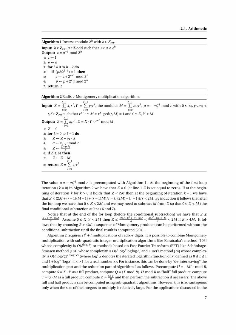
Algorithm 2 Radix-r Montgomery multiplication algorithm.

Input: X =`−1∑i=0

xi r i ,Y =`−1∑i=0

yi r i , the modulus M =`−1∑i=0

mi r i , µ = −m−10 mod r with 0 ≤ xi , yi ,mi <

r,` ∈ Z>0 such that r `−1 ≤ M < r `, gcd(r, M) = 1 and 0 ≤ X ,Y < M

Output: Z =`−1∑i=0

zi r i , Z = X ·Y · r−` mod M

1: Z ← 02: for k = 0 to `−1 do3: Z ← Z + yk ·X4: q ← z0 ·µ mod r

5: Z ← Z+q ·Mr

6: if Z ≥ M then7: Z ← Z −M

8: return Z =`−1∑i=0

zi r i

The value µ = −m−10 mod r is precomputed with Algorithm 1. At the beginning of the first loop

iteration (k = 0) in Algorithm 2 we have that Z = 0 (at line 1 Z is set equal to zero). If at the begin-

ning of iteration k for k > 0 it holds that Z < 2M then at the beginning of iteration k + 1 we have

that Z < (2M + (r −1)(M −1)+ (r −1)M)/r = (r (2M)− (r −1))/r < 2M . By induction it follows that after

the for loop we have that 0 ≤ Z < 2M and we may need to subtract M from Z so that 0 ≤ Z < M (the

final conditional subtraction at lines 6 and 7).

Notice that at the end of the for loop (before the conditional subtraction) we have that Z ≤X Y +(R−1)M

R . Assume 0 ≤ X ,Y < 2M then Z ≤ (2M−1)2+(R−1)MR < 4M 2+(R−1)M

R < 2M if R > 4M . It fol-

lows that by choosing R > 4M , a sequence of Montgomery products can be performed without the

conditional subtraction until the final result is computed [204].

Algorithm 2 requires 2l 2 + l multiplications of radix-r digits. It is possible to combine Montgomery

multiplication with sub-quadratic integer multiplication algorithms like Karatsuba’s method [108]

whose complexity is O(`log2 3) or methods based on Fast Fourier Transform (FFT) like Schönhage-

Strassen method [181] whose complexity is O(` log` loglog`) and Fürer’s method [74] whose complex-

ity is O(` log`)2O(log∗ `) (where log∗ x denotes the iterated logarithm function of x, defined as 0 if x ≤ 1

and 1+ log∗ (log x) if x > 1 for a real number x). For instance, this can be done by “de-interleaving” the

multiplication part and the reduction part of Algorithm 2 as follows. Precompute U =−M−1 mod R,

compute S = X · Y as a full product, compute Q = (T mod R) ·U mod R as “half” full product, compute

T =Q ·M as a full product, compute Z = S+TR and then perform the subtraction if necessary. The above

full and half products can be computed using sub-quadratic algorithms. However, this is advantageous

only when the size of the integers to multiply is relatively large. For the applications discussed in the

7


following chapters Algorithm 2 is the most efficient.

Algorithm 3 shows the binary left-to-right modular exponentiation method [113, 4.6.3] modified

to use Montgomery arithmetic (and Algorithm 2 as a sub-routine), which requiresΘ(k) Montgomery

multiplications for a k-bit exponent E ∈ Z>0. There exist other modular exponentiation techniques.

For instance the sliding window method [8, 9.1.3] reduces the number of modular multiplications

performed at the price of some pre-computation and memory storage and the Montgomery ladder [144]

provides resistance to some side-channel attacks [117].

Algorithm 3 Radix-r binary left-to-right “Montgomery” exponentiation.


xi r i , the modulus M =`−1∑i=0

mi r i and E =k−1∑j=0

e j 2 j with e j ∈ {0,1}, k ∈ Z>0, ek−1 = 1,

0 ≤ xi ,mi < r,` ∈ Z>0 such that r `−1 ≤ M < r `, gcd(r, M) = 1, R = r ` and 0 ≤ X < MOutput: Z = X E mod M

1: X ← X ·R2 mod M2: Z ← X3: for j = k −2 downto 0 do4: Z ← Z ·Z5: if e j = 1 then6: Z ← Z · X7: Z ← Z ·18: return Z =

`−1∑i=0

zi r i

2.4.2 Exact division

Algorithm 4 shows the exact division method originally proposed in [104] to compute Y /X with

X ∈ Z>0, Y ∈ Z≥0 and X | Y . The method avoids division using the fact that X | Y . If Z = Y /X then

Z X ≡ z0x0 ≡ y0 mod r so z0 can be computed as z0 = (x−10 · y0) mod r . The algorithm iteratively

computes the other digits of the quotient using the facts that if Tk = Y −k−1∑h=0

zh X r h and in radix-r

representation Tk =m−1∑i=0

ti with 0 ≤ k ≤ m −n then tk ≡ zk+1x0 mod r ⇒ zk+1 ≡ tk x−10 mod r and

that Tk ≡ 0 mod r k+1. Notice that computing Tm−n = Y −Z X = 0 is not needed so the computation of

zm−n is performed outside the for loop at line 5.

The similarity with the Montgomery multiplication algorithm (see Algorithm 2) is evident.

2.4.3 A divisibility test

Algorithm 5 illustrates a “division free” method to test the divisibility of a radix-r integer X by an integer

0 < d < r with gcd(d ,r ) = 1. This method can be thought of as a variant of the exact division method

described in 2.4.2. The main observation in this case is that if r |X then d |X if and only if d | Xr . The idea

of the algorithm is to use Montgomery multiplication’s trick (see subsection 2.4.1 for the details) to

iteratively add kd for some k ∈ Z≥0 to X (the result will still be equal to X modulo d) such that X +kd

is divisible by r (or equivalently X +kd ≡ 0 mod r ) and replace X with X+kdr until X < r . At this point it

is enough to check whether X = 0 or not to determine whether the input X is divisible by d .

8

2.4. Arithmetic

Algorithm 4 Radix-r exact division [104].

Input: X =n−1∑i=0

xi r i ,Y =m−1∑i=0

yi r i with 0 ≤ xi , yi < r,m ≥ n > 0 such that X | Y and gcd(x0,r ) = 1

Output: Z = Y /X =m−n∑i=0

zi r i with 0 ≤ zi < r

1: x ′ ← x−10 mod r

2: for k = 0 to m −n −1 do3: zk ← x ′ · y0 mod r

4: Y ← Y − zk ·X

r5: zm−n ← x ′ · y0 mod r

6: return Z =m−n∑i=0

zi r i

Algorithm 5 Radix-r divisibility test.


xi r i with 0 ≤ xi < r , an integer d < r with gcd(d ,r ) = 1 and ` ∈ Z>0

Output: Return T RU E if d |X and F ALSE otherwise1: µ←−d−1 mod r2: x ′ ← x0

3: xl ← 0 // “Pad” X with an extra 0 digit4: for i = 1 to l do5: k ← (x ′ ·µ) mod r

6: Z ← (x′+k·dr // Z < 2d

7: if Z ≥ d then8: Z ← Z −d9: Z ← (Z +xi ) // Z < r +d

10: if Z ≥ r then11: Z ← Z −d12: x ′ ← Z13: if x ′ = 0 then14: return T RU E15: else16: return F ALSE

2.4.4 A compositeness test: Miller-RabinTheorem 1 (Fermat’s little theorem). Given a, p ∈ Z with p prime and p 6 |a, we have that

ap−1 ≡ 1 mod p

or equivalently that ap−1 −1 is an integer multiple of p. If we do not impose p 6 |a, then we have that

ap ≡ a (mod p)

instead or equivalently that ap −a is an integer multiple of p.

Given positive integers n and a (base) such that gcd(a,n) = 1, compute b = an−1 mod n. If b 6=1 mod n then n fails the “Fermat test” and so it is composite by Theorem 1 (a is said to be a “witness” to

the compositeness of n). Otherwise we say that n is “pseudoprime” to the base a. From Fermat’s little

theorem we know that a prime n will be pseudoprime to all bases a (positive integers with gcd(a,n) = 1),

9


but unfortunately there exist also composite numbers pseudoprime to all bases a, the Carmichael

numbers [50]. There exist infinitely many Carmichael numbers [1], although as n grows, they occur

much less often than primes [172]. Abstractly, Theorem 1 states that if n is prime then a certain equality

is satisfied. Fermat’s test uses the contrapositive of this implication, namely if the equality is not

satisfied by n then n is not a prime. As a consequence it is not a primality test, but a compositeness test.

The Miller-Selfridge-Rabin pseudoprimality test [6, 140, 176] is based on Theorem 2, which follows

from Fermat’s little theorem and the fact that if n is prime then the equation x2 = 1 mod n has only two

solutions in Z/nZ: x = 1 and x =−1.

Theorem 2. If n is an odd prime such that n − 1 = 2s t with t odd and a is a positive integer with

gcd(a,n) = 1 then one of the two following conditions must hold:{at = 1 mod n

a2i t =−1 mod n for some i with 0 ≤ i ≤ s −1

If n fails the above test, i.e., none of the above conditions hold, then n is composite and a is a

witness to the compositeness of n. Otherwise if n passes the test we say that n is a “strong pseudoprime”

to the base a. Unlike Fermat’s test, there does not exist a composite n being a strong pseudoprime

to all bases a with gcd(a,n) = 1. It can be shown [142], [176] that for each composite integer n with

n > 9 the number of integers a with 0 < a < n such that n is a “strong pseudoprime” to the base a

is at most φ(n)4 . It follows that the probability that a uniformly random base a with 0 < a < n is a

witness to the compositeness of n is larger than (n − φ(n)4 )/n > (n − n

4 )/n = 3/4. This result gives rise

to Algorithm 6. On input an odd composite integer n > 9 and a positive integer k Algorithm 6 returns

strong pseudoprime with probability less than(1− 3

4

)k = 14k . The choice a = 2 allows to replace some

modular multiplications needed to computer the modular exponentiation on line 4 (e.g., Montgomery

multiplications computed at line 6 of Algorithm 3) with cheaper modular additions and in practice one

iteration (i.e., setting k = 1) suffices to recognize “most” composites quickly.

Algorithm 6 Miller-Selfridge-Rabin compositeness test

Input: An odd integer n to be tested such that n > 3 and a positive integer kOutput: Either composite or strong pseudoprime

1: Write n −1 as n −1 = 2s t where t is odd2: for i = 1 to k do3: Pick a random integer (base) a such that 1 < a < n −14: b ← at mod n5: if b 6≡ ±1 mod n then6: j ← 17: while ( j < s)∧ (b 6≡ −1 mod n) do8: b ← b2 mod n9: if b ≡ 1 mod n then

10: return composite11: j ← j +112: if b 6≡ −1 mod n then13: return composite14: return strong pseudoprime

10

2.5. Elliptic curves and genus 2 hyperelliptic curves

2.5 Elliptic curves and genus 2 hyperelliptic curvesIn this section we introduce the basic facts about elliptic curves and hyperelliptic curves that are needed

in this thesis.

2.5.1 Weierstrass curvesWe use an informal definition of elliptic curves for the sake of simplicity in line with [130] and we refer

the reader to [190, Chapter III] for a general and more formal introduction. We denote by K a field with

characteristic different from 2,3. An elliptic curve E over K is then defined by a short affine Weierstrass

equation (2.1)

y2 = x3 +ax +b (2.1)

with a,b ∈ K and 4a3 +27b2 6= 0. The set of points E(K ) of the elliptic curve E over K is defined as

E(K ) = {(x, y) ∈ K 2 such that y2 = x3 +ax +b}∪ {O(point at infinity)}. (2.2)

Such a set of points has the structure of an abelian group with the point at infinity O being the identity

element. The group law is defined as follows (in additive notation):

• Identity element: O +P = P +O = P for all P ∈ E(K ).

• Negative element: Given P = (x1, y1) 6=O and Q = (x2, y2) 6=O we have that P +Q =O if and only

if x1 = x2 and y1 =−y2; thus −(x, y) = (x,−y).

• Addition and doubling: Given λ ∈ K such that λ= (y1 − y2)/(x1 −x2) if P 6=Q (therefore x1 6= x2)

or λ= (3x21 +a)/(2y1) if P =Q, we have that P +Q = R, where R = (x3, y3) with x3 = λ2 − x1 − x2

and y3 =−λx3 − y1 +λx1.

We note that adding two distinct points and adding a point with “itself” (doubling) are different

operations and that the point at infinity has no concrete representation in this coordinate system. The

system of coordinates used above is usually referred to as affine Weierstrass coordinates. We use the

following abbreviations to express the cost of elliptic curve operations in terms of finite field operations:

a for field addition (or subtraction), m for field multiplication, s for field squaring, i for field inversion

and c for multiplication by a constant depending on the curve equation. The cost of addition in

Weierstrass affine coordinates is then 2m+1s+6a+1i and the cost of doubling is 2m+2s+7a+1i.It is possible to use different coordinate systems with faster addition and doubling formulae than

affine coordinates. For example, addition and doubling in Weierstrass projective coordinates require

more field operations but avoid the inversion [60, Chapter 7]. In software a field inversion is usually

significantly slower than field multiplication. When using projective coordinates the set of points E(K )

of E over K is defined by equation (2.3)

E(K ) = {(x : y : z) ∈P2(K ) : y2z = x3 +axz2 +bz3} (2.3)

where P2(K ) denotes the projective plane over K , i.e., the set of equivalence classes of triples (x, y, z) ∈K 3, (x, y, z) 6= (0,0,0); two triples (x, y, z) and (x ′, y ′, z ′) are equivalent if there exists c ∈ K ∗ such that

cx = x ′, c y = y ′ and cz = z ′. The equivalence class containing (x, y, z) is denoted by (x : y : z). Given

an elliptic curve E over K , the point (0 : 1 : 0) ∈ E(K ) is the point at infinity and it is the only point for

which z = 0. All the other points of E are of the form (x : y : 1), where x, y ∈ K satisfy equation (2.1).

In several cases the operation to optimize is scalar multiplication of a point P by a scalar k ∈ Z>0

defined as P +P +·· ·+P︸︷︷︸k

. The double-and-add method to perform scalar multiplication is shown in

11


Algorithm 7. This method performs Θ(k) elliptic curve operations for k-bit exponent K ∈ Z>0. It is

analogous to Algorithm 3 for modular exponentiation and methods like sliding-window exponentiation

or the Montgomery ladder mentioned in Section 2.4.1 can be easily adapted to scalar multiplication.

Algorithm 7 Double-and-add elliptic curve scalar multiplication.

Input: P ∈ E(Fp ) and K =`−1∑j=0

e j 2 j with e j ∈ {0,1}, e`−1 = 1, and ` ∈ Z>0

Output: Q = K ·P with Q ∈ E(Fp )1: Q ← P2: for j = l −2 downto 0 do3: Q ← 2Q4: if e j = 1 then5: Q ←Q +P6: return Q

In addition to varying the coordinate system, one can also use curve models defined by different

equations.

2.5.2 Montgomery curvesEquation (2.4) defines a Montgomery curve. This family of curves was introduced by Peter Mont-

gomery [144].

B y2 = x3 + Ax2 +x, (2.4)

with A2 6= 4 and B 6= 0. The set of points of a Montgomery curve over a field K and the notion of

projective coordinates are defined analogously to the case of Weierstrass curves. Montgomery curves

provide faster arithmetic than Weierstrass curves for all the applications in which the y coordinate of

points can be dropped. This is means that points are identified up to their sign, but despite that, it is

still possible to compute scalar multiplication.

For all nonzero λ ∈ K , the point (X : Y : Z ) = (λX : λY : λZ ) corresponds to the affine point

(X /Z ,Y /Z ) ∈ E (K ) with Z 6= 0, x = X /Z and y = Y /Z satisfying equation (2.4). Given two distinct points

in projective coordinates P = (X1 : Y1 : Z1),Q = (X2 : Y2 : Z2), and their difference P −Q = (X4 : Y4 : Z4), it

is possible to derive efficient formulae for computing the X and Z projective coordinates of their sum

R = P +Q = (XS : YS : ZS ), that do not involve Y coordinates:

XS = Z4 · [(X1 −Z1)(X2 +Z2)+ (X1 +Z1)(X2 −Z2)]2,

ZS = X4 · [(X1 −Z1)(X2 +Z2)− (X1 +Z1)(X2 −Z2)]2.

These addition formulae can be computed at the cost of 4m+2s+6a by caching some intermediate

values.

Similarly given P = (X1 : Y1 : Z1) and 2P = (XD : YD : ZD ) we have:

4X1Z1 = (X1 +Z1)2 − (X1 −Z1)2, XD = (X1 +Z1)2(X1 −Z1)2,

ZD = (4X1Z1)[(X1 −Z1)2 + ((A+2)/4)(4X1Z1)],

These doubling formulae can be computed at the cost of 3m+2s+4a+1c by caching some intermediate

values.

As the addition formulae require the difference of two input points, the scalar multiplication

(Q = kP for a positive integer k) is performed using a special case of addition chains called Lucas

12

2.5. Elliptic curves and genus 2 hyperelliptic curves

chains [145]. An addition chain for n ∈ Z>0 is a sequence of positive integer values v0 = 1, v1, . . . , vm = n

with m ∈ Z>0), where for each 0 < j ≤ m, v j = vh + vl for some 0 ≤ h, l < j .

2.5.3 Edwards curves

The curves providing the fastest scalar multiplication are, as of today, Edwards curves originally intro-

duced by Edwards in 2007 as a normal form for elliptic curves [67]. A more general version of these

curves was introduced by Bernstein and Lange together with the first algorithm to compute point

addition in projective coordinates whose cost is 10m+1s+7a+2c [23]. The latter curves are today

known as Edwards curves. Bernstein and Lange introduced also inverted Edwards coordinates resulting

in a point addition cost of 9 m+1s+7a+3c [24]. Later, Bernstein et al. introduced a generalization of

Edwards curves, namely twisted Edwards curves [14] and finally the fastest group arithmetic for twisted

Edwards was introduced by Hisil et al. [99] with the use of an additional coordinate, i.e., the extended

twisted Edwards coordinate system.

Let K be a field of odd characteristic, Edwards curves are defined by equation (2.5)

x2 + y2 = c2(1+d x2 y2) (2.5)

where c,d ∈ K with cd(1−dc4) 6= 0. This form is a special case of the more general twisted Edwards

curve form defined by equation (2.6)

ax2 + y2 = 1+d x2 y2 (2.6)

where a,d ∈ K with ad(a −d) 6= 0 (Edwards curves represent the special case where a can be rescaled

to 1). Group operation formulae for these curves can be found in [14]. The set of points of a twisted

Edwards curve over a field K and the notion of projective coordinates are defined analogously to the

case of Weierstrass curves. In projective coordinates the point at infinity is (0 : 1 : 1) and the negative

of (X : Y : Z ) is (−X : Y : Z ). For all λ 6= 0 ∈ K , (X : Y : Z ) = (λX : λY : λZ ). This projective coordinate

system for twisted Edwards curves is denoted by E .

In the extended coordinate system a new coordinate t = x y is introduced to represent a point

(x, y) in E(K ) where E is defined by equation (2.6) in extended affine coordinates as (x, y, t ). The map

(x, y, t) → (x : y : t : 1) allows to move to projective coordinates. For all nonzero λ ∈ K , the point (X :

Y : T : Z ) = (λX : λY : λT : λZ ) corresponds to the extended affine point (X /Z ,Y /Z ,T /Z ) ∈ E(K )

with Z 6= 0, x = X /Z and y = Y /Z satisfying equation (2.6). For the auxiliary coordinate T it holds

that T = X Y /Z . This system is called extended twisted Edwards coordinates and is denoted by E e .

The point at infinity is (0 : 1 : 0 : 1). The negative of (X : Y : T : Z ) is (−X : Y : −T : Z ). Given (X ,Y , Z )

in E , passing to E e costs 3m+1s by computing (X Z ,Y Z , X Y , Z 2) whereas given (X : Y : T : Z ) in E e

passing to E is cost-free by simply dropping T . Given two distinct points P = (X1 : Y1 : T1 : Z1),Q =(X2 : Y2 : T2 : Z2) ∈ E(K ) with E defined by equation (2.6) represented in E e with Z1 6= 0 and Z2 6= 0 their

sum R = P +Q = (XS : YS : TS : ZS ) is computed as:

XS = (X1Y2 −Y1X2)(T1Z2 +Z1T2),

YS = (Y1Y2 +aX1X2)(T1Z2 −Z1T2),

TS = (T1Z2 +Z1T2)(T1Z2 −Z1T2),

ZS = (Y1Y2 +aX1X2)(X1Y2 −Y1X2).

These addition formulae are independent of the curve constant d and can be computed at the cost

13


of 9m+7a+1c. Whereas 2P = (XD : YD : TD : ZD ) with P = (X1 : Y1 : T1 : Z1) ∈ E(K ) is computed as:

XD = 2X1Y1(2Z 21 −Y 2

1 −aX 21 ),

YD = (Y 21 +aX 2

1 )(Y 21 −aX 2

1 ),

TD = 2X1Y1(Y 21 −aX 2

1 ),

ZD = (Y 21 +aX 2

1 )(2Z 21 −Y 2

1 −aX 21 ).

These doubling formulae are also independent of the curve constant d and can be computed at the

cost of 4m+4s+8a+1c. Formulae for mixed addition, namely for adding a point in affine coordinate

to a point in projective coordinates can be derived setting Z2 = 1. If a =−1 then the multiplication by

the curve constant a can be saved and one further multiplication can be saved if Z2 = 1. The cost can

be reduced by mixing E e with E . Notice that the cost of these formulae is higher than the cost of the

formulae presented in [14] (i.e., 3m+4s+8a+1c).

Twisted Edwards curves are endowed also with unified and complete addition formulae. Unified

addition formulae compute R = P +Q correctly even if P = Q (i.e., they can be used for doubling).

Complete addition formulae are defined for all inputs, i.e., without exceptions for doubling, the neutral

element and negatives. This type of addition formulae are desirable in cryptography as they prevent

some side-channel attacks [103].

We now sketch the mixed scalar multiplication method presented in [99]. This elliptic curve scalar

multiplication method is to date the fastest known in literature. The basic idea is to mix E e and E and

use the fact that no consecutive additions are computed. As a result it is possible to replace slower

doublings in E e with faster doublings in E :

1. If a point doubling is followed by another point doubling, use E ← 2E .

2. If a point doubling is followed by a point addition, use

(a) E e ← 2E for the doubling step and then,

(b) E ← E e +E e for the point addition step.

E ← 2E is performed using the faster formulae (3m+4s+8a+1c) presented in [14]. The operation

E e ← 2E is obtained by simply using the doubling formulae in E e mentioned above as they do not

require the input coordinate T1 and result in a cost-free conversion to E e . The formulae for addition in

E e shown above are used for E ← E e +E e . The computation of TS can be avoided. This offsets the extra

field multiplication necessary to compute TD in E e ← 2E .

2.5.4 Genus 2 hyperelliptic curvesWe give a brief overview of genus 2 hyperelliptic curves describing the basic concepts used in Chapter 4.

A genus 2 hyperelliptic curve over a field of odd characteristic K is defined by an equation C : y2 = f (x)

where f (x) is a polynomial of degree 5 or 6 with no double roots. We assume for the remainder of this

thesis that a genus 2 hyperelliptic curve is defined by equation 2.7.

C : y2 = x5 + f3x3 + f2x2 + f1x + f0. (2.7)

The set of points C (K ) of C over K (defined in the same way as for elliptic curves, cf. equation (2.2)) is

not endowed with a group structure, however roughly speaking, a group structure can be constructed

by considering “pairs” of points as group elements. Formally we need to use the Jacobian of C , Jac(C ),

consisting of degree zero divisors on C modulo principal divisors (see [8, Chapter 4] for more details).

Points of the Jacobian group in this case are weight 2 divisors. Such divisors can be represented in

14

2.6. Integer factorization algorithms

Mumford representation [152] as (u(x), v(x)) = (x2 +u1x +u0, v1x + v0) ∈ K [x]×K [x], such that u(x1) =u(x2) = 0, v(x1) = y1 and v(x2) = y2, where (x1, y1) and (x2, y2) are two (not necessarily distinct) points

in the set C (K ), and y1 6= −y2. Formulae for both addition and doubling of points of Jac(C ) for C over

finite fields exist in different coordinate systems and are analogous to addition and doubling formulae

for elliptic curves. Addition and doubling formulae in affine coordinates are shown in Table 2.1 where a

point P ∈ Jac(C ) is represented in Mumford affine coordinates as P = (u1,u0, v1, v0,U1 = u21,U0 = u1u0).

Algorithm 7 can be used to compute kP for P ∈ Jac(C ) and a positive integer k.

Mumford affine additionInput: P1 = (u1,u0, v1, v0,U1 = u2

1,U0 = u1u0), P2 = (u′1,u′

0, v ′1, v ′

0,U ′1 = u′2

1 ,U ′0 = u′

1u′0),P1,P2 ∈ Jac(C )

σ1 ← u1 +u′1, ∆0 ← v0 − v ′

0, ∆1 ← v1 − v ′1, M1 ←U1 −u0 −U ′

1 +u′0, M2 ←U ′

0 −U0,

M3 ← u1 −u′1, M4 ← u′

0 −u0, t1 ← (M2 −∆0) · (∆1 −M1), t2 ← (−∆0 −M2) · (∆1 +M1),

t3 ← (−∆0 +M4) · (∆1 −M3), t4 ← (−∆0 −M4) · (∆1 +M3),

`2 ← t1 − t2 `3 ← t3 − t4, d ← t3 + t4 − t1 − t2 −2(M2 −M4) · (M1 +M3),

A ← 1/(d ·`3), B ← d · A, C ← d ·B , D ← `2 ·B , E ← `23 · A, CC ←C 2,

u′′1 ← 2D −CC −σ1, u′′

0 ← D2 +C · (v1 + v ′1)− ((u′′

1 −CC ) ·σ1 + (U1 +U ′1))/2,

U ′′1 ← u′′2

1 , U ′′0 ← u′′

1 ·u′′0 , v ′′

1 ← D · (u1 −u′′1 )+U ′′

1 −u′′0 −U1 +u0,

v ′′0 ← D · (u0 −u′′

0 )+U ′′0 −U0, v ′′

1 ← E · v ′′1 + v1 v ′′

0 ← E · v ′′0 + v0.

Output: R = P1 +P2 = (u′′1 ,u′′

0 , v ′′1 , v ′′

0 ,U ′′1 = u′′2

1 ,U ′′0 = u′′

1 u′′0 ),R ∈ Jac(C ).

Cost: i+17m+4s + 48a

Mumford affine doublingInput: P1 = (u1,u0, v1, v0,U1 = u2

1,U0 = u1u0), with constants f2, f3 ∈ K (see equation (2.7)), P1 ∈ Jac(C )

v v ← v21 , vu ← (v1 +u1)2 − v v −U1, M1 ← 2v0 −2vu, M2 ← 2v1 · (u0 +2U1),

M3 ←−2v1, M4 ← vu +2v0, z1 ← f2 +2U1 ·u1 +2U0 − v v, z2 ← f3 −2u0 +3U1,

t1 ← (M2 − z1) · (z2 −M1), t2 ← (−z1 −M2) · (z2 +M1),

t3 ← (M4 − z1) · (z2 −M3), t4 ← (−z1 −M4) · (z2 +M3),

`2 ← t1 − t2, `3 ← t3 − t4, d ← t3 + t4 − t1 − t2 −2(M2 −M4) · (M1 +M3),

A ← 1/(d ·`3), B ← d · A, C ← d ·B , D ← `2 ·B , E ← `23 · A,

u′′1 ← 2D −C 2 −2u1, u′′

0 ← (D −u1)2 +2C · (v1 +C ·u1), U ′′1 ← u′′2

1 , U ′′0 ← u′′

1 ·u′′0 ,

v ′′1 ← D · (u1 −u′′

1 )+U ′′1 −U1 −u′′

0 +u0, v ′′0 ← D · (u0 −u′′

0 )+U ′′0 −U0,

v ′′1 ← E · v ′′

1 + v1, v ′′0 ← E · v ′′

0 + v0.

Output: R = 2P1 = (u′′1 ,u′′

0 , v ′′1 , v ′′

0 ,U ′′1 = u′′2

1 ,U ′′0 = u′′

1 u′′0 ),R ∈ Jac(C ).

Cost: i+19m+6s + 52a

Table 2.1 – Addition and doubling in the Jacobian group of a hyperelliptic curve C defined over an oddcharacteristic field K in Mumford affine coordinates.

2.6 Integer factorization algorithmsIn this section we describe some of the integer factoring algorithms we use in the following chapters. In

particular we give details about the factoring algorithms used in the post-sieving phase of the number

15


field sieve (NFS) as they are used in Chapter 3. We also give a very high level overview of the structure

of the NFS. This structure is common to several simpler factoring algorithm like the quadratic sieve

(QS) and touch upon the aspects in which the NFS differs. For a comprehensive description of NFS we

refer the reader to [128]. We denote by n the positive composite integer we want to factor and assume

that n is not a prime power (this can be checked in polynomial time in logn).

2.6.1 Trial divisionThe most naive trial division method consists in simply trying to divide n by all d ∈ Z≥2 such that d ≤p

n,

or more in general d ≤ B ≤pn for a desired positive upper bound B (we might aim to detect factors

only up to a certain size). To find a factor of n (or declare it as prime), the number of trial divisions

required is aboutp

n in the worst case. It is trivial to do better: if the number is odd or the 2’s factors

are first removed, then it drops top

n2 by trial dividing for odd numbers only. This improvement can be

regarded as a trivial example of “prime wheel”. To use a prime wheel we first multiply together primes

pi not larger than a fixed positive integer bound Bw ≤ B , i.e., we compute M = ∏pi≤Bw

pi with pi prime.

Then we compute all mi ∈ Z>0 such that gcd(M ,mi ) = 1 and mi ≤ M , where 0 ≤ i <φ(M) with φ(M)

denoting the Euler’s totient function of M . For each consecutive pair mi+1,mi with 0 ≤ i <φ(M)−1 we

store the difference δi = mi+1 −mi and also δφ(M)−1 = m0 −mφ(m)−1 mod M in a table. After we trial

divide by the primes dividing M we set d = 1 and we iteratively trial divide by d ← d +δ(i ) mod φ(M) for

i = 0,1, . . . until d > B . By doing so we only trial divide by values not divisible by the primes dividing

M and avoid useless trial divisions. If we have enough memory we can do better by preparing a list of

primes p such that 2 ≤ p ≤ B (or just the difference of each pair of consecutive primes in the interval)

and then trial divide just by every prime in the list. If B =pn this requires π(

pn) ≈

pn

logp

nby the prime

number theorem. Each trial division can be performed in different ways, for instance:

1. Use a division algorithm computing both quotient and remainder, and check whether the latter

is 0 or not.

2. Take the gcd of n and the candidate divisor and if it is larger than 1 use an exact division algorithm.

3. Use a divisibility test and then use exact division algorithm if needed.

If we are interested in testing whether an integer n is prime or not, or which are the primes appearing

in its factorization we can directly use one of the above variations. If we need to find the full prime

factorization of n then every time we find a divisor d we have to repeatedly compute n ← n/d until

d 6 |n to find its multiplicity. Similarly we can check if the number n is B-smooth or B-powersmooth for

a positive integer bound B .

2.6.2 Pollard p −1Pollard’s p −1 method for integer factorization [169] is an application of Fermat’s little theorem (see

Theorem 1). On input a composite integer n, the method works as follows. Select an arbitrary integer

a such that a 6= ±1 and gcd(a,n) = 1 (otherwise, we can immediately factor n). Fix a positive integer

bound B1 and compute the value R = ∏pi≤B1

pblogpi

B1ci with pi prime, namely R is the product of all

prime powers less than B1. Calculate b = aR mod n and then g = gcd(b −1,n). The method succeeds if

1 < g < n, in which case g is a proper divisor of n.

Notice that R does not have to be calculated explicitly and the computation of b = aR mod n can be

carried out in O(logR) =O(B1) operations modulo n with classic modular exponentiation algorithms

(see Section 2.4.1). Assume p is a prime divisor of n, by Fermat’s little theorem it follows that if p −1|Rthen b ≡ 1 mod p and so p|gcd(b−1,n). Therefore, if for some prime divisor p of n the value p −1 (i.e.,

16


the order of the multiplicative group of residues modulo p, i.e., (Z/pZ)∗) is B1-powersmooth then g

will be larger than 1. As mentioned above, the method succeeds if 1 < g < n, whereas if g = n it is likely

that B1 is too large (for each prime factor p of n the value p −1 is B1-powersmooth) and we can reduce

it and retry with the resulting smaller R. If g = 1 then the method has failed and we can abandon it, or

increase B1 and retry, or perform the so called stage 2 [144]. In stage 2, we assume that for some prime

factor p of n the value p −1 is B1-powersmooth except for one prime s such that B1 < s < B2 where B2

is a second integer bound larger than B1. In other words, we assume that p −1 =Qs where Q|R and s

is the outlying prime. Since (p −1)|Rs it follows by Fermat’s little theorem that if cs = bs ≡ aRs mod n

then p|(cs −1) and p|gcd(cs −1,n). In stage 2 we look for such prime s.

Let s j denote the j -th prime. The standard stage 2 computes cs j for each B1 ≤ s j ≤ B2 and checks if

gcd(cs j ,n) > 1 for each cs j . The sequence of gcd computations can be avoided by multiplying together

the values cs j , i.e., calculating W =∏cs j , and then checking if gcd(W,n) > 1. In practice the difference

of consecutive primes is small and this can be used to compute each cs j as follows. For each pair of

consecutive primes (s j , s j+1) in [B1,B2] compute bs j+1−s j mod n and store it in a table. If the largest

difference is D, compute b2 j mod n for 1 ≤ j ≤ D/2 (the difference of two primes is even) and store

each value in a look-up table. This pre-computation requires D/2 multiplications and memory space

for D/2 values.

Then compute cs1 = bs1 mod n where s1 is the smallest prime in [B1,B2], with O(log s1) modular

multiplications. Finally for each prime B1 ≤ s j ≤ B2 compute cs j = bs j mod n as c j−1 ·bs j −s j−1 mod n,

namely as the product of the partial result corresponding to the current prime and the value in the

look-up table corresponding to the difference between the next and the current prime, and then W =∏cs j . For each prime, two multiplications are needed (one for the above computation and one for

accumulating the result if the gcd with n is computed at the end). As a result 2(π(B2)−π(B1)) ≈2(

B2logB2

− B1logB1

)+D/2 multiplications are performed in this last step.

We can do better using a different time-memory trade-off known as baby-step giant-step (BSGS).

The idea is to write each prime s such that B1 ≤ s ≤ B2 in radix w as s = t w −u where w ≈ pB2,

t1 ≤ t ≤ t2 with t1 =⌈

B1w

⌉, t2 =

⌈B2w

⌉. Now we precompute the values bu mod n, the “baby steps”, for

0 ≤ u < w and store them into a table. Then we can compute the values bt w mod n for t1 ≤ t ≤ t2,

the “giant steps”, and store them in a table or we can simply process primes in ascending order and

compute the values as they are needed. Notice that if s = t w −u, gcd(bs −1,n) = gcd(bt w −bu ,n). Thus,

for each prime s = t w −u in [B1,B2] we compute the value bt w −bu mod n and we can accumulate

it by multiplying with the previous ones as before and compute one gcd with n at the end. With this

approach we need aboutp

B2 multiplications to compute the baby steps, and O(log w+log t1+t2−t1) =O

(log

pB2 + log

⌈B1pB2

⌉+⌈p

B2⌉−⌈

B1pB2

⌉)= O(

pB2) multiplications to compute the giant steps.The

number of multiplications needed for the final step is π(B2)−π(B1) ≈(

B2logB2

− B1logB1

). If B2 and B1 are

large enough we can roughly halve the number of multiplications compared to the previous approach.

Advanced Pollard p−1 BSGS stage 2. We can offset some of the baby steps pre-computations (and con-

sequently stored values) not corresponding to any prime, if we consider only values of u with gcd(u, w) =1. It follows that choosing the radix w as the product of small primes close to

pB2 we can offset more

values. Smaller values of w can also be tried and in general the optimal choice has to be found

experimentally.

We can reduce the number of multiplications in the final step at the cost of some extra pre-

computations. Assume we can find values (t ,u) as before with the additional property that we can

represent pairs of primes B1 ≤ si , s j ≤ B2 as si = t w +u and s j = t w −u. We can check two primes

in one pair “at once” if we slightly modify the values computed in the final step. Namely, for each

prime pair we compute b(t w)2 −b(u)2mod n since if s is the outlying prime we are looking for and

s|t w ±u|(t w)2 − (u)2 then p|bs −1|b(t w)2 −b(u)2. To compute efficiently the baby steps and the giant

17


Algorithm 8 Evaluate b(x)2mod n at x = k + i h for i = 0,1,2, . . . , l with ` ∈ Z≥0.

Output: C = {ci = b(k+i h)2mod n for i = 0,1,2, . . . , l }

1: c0 ← b(k)2mod n, c1 ← b(k+h)2

mod n, c2 ← b(k+2h)2mod n

2: e0 ← c0

3: e1 ← c1 · (c0)−1 mod n = b(2kh+h2) mod n4: e2 ← c2 · (c1)−1 · (e1)−1 mod n = b(2h2) mod n5: c ← e0

6: C ← {e0}7: for i = 0 to l do8: c ← c ·e1 mod n9: e1 ← e1 ·e2 mod n

10: C ←C ∪ {c}11: return C

steps we observe that both the u values and the t w values are in an arithmetic progression. We can

efficiently evaluate b(k+i h)2mod n for i = 0,1,2, . . . where k is the first integer value of the arithmetic

progression and h is the positive integer difference of consecutive values.

As shown in Algorithm 8, after some extra pre-computations we can calculate the baby step and the

giant step values at the cost of only one additional multiplication per value with respect to the previous

approach. As far as the bounds for the u values and t values are concerned we have that t1 ≤ t ≤ t2

with t1 =⌊

B1w

⌋, t2 =

⌈B2w

⌉and u ≤ umax with umax ≥ w

2 . The cost of the algorithm is proportional to

the number of prime pairs to be checked. If π(B2)−π(B1) is much larger than t2 − t1 and umax , the

overall cost is mainly determined by the number of prime pairs to be checked, which is lower bounded

by π(B2)−π(B1)2 in the ideal case in which every prime is paired with another prime. A larger value for

umax allows to pair a larger number of primes and consequently reduce the number of pairs to be

checked, but the practical effect on the performance has to be verified because it may increase the

number of memory accesses.

Other flavors of stage 2 and optimization tricks for relatively large bounds B1 and B2 can be found

in [144, 148].

2.6.3 ECMThe elliptic curve method (ECM) for integer factorization was proposed by Hendrik Lenstra in 1985 [130].

ECM can be derived from Pollard’s (p −1)-method (see Section 2.6.2) conceptually “replacing” the

multiplicative group of residues modulo p ((Z/pZ)∗) with the group of points on a random elliptic

curve E defined over Z/pZ. We recall that p is an unknown prime divisor of the composite integer n we

want to factor. Fix a positive integer bound B1 and compute the value k = ∏pi≤B1

pblogpi

B1ci with pi prime

as in Pollard p −1. Select the coordinates of a point P at random (in Z /nZ) and then an elliptic curve E

defined over Z/nZ such that P ∈ E(Z/nZ), where n is the integer to factor. Next, compute the multiple

k ·P of P with a scalar multiplication. Notice that the algorithm works with elliptic curves defined over

the finite ring Z/nZ. The set of points of an elliptic curve defined over a finite ring is still endowed

with a group structure, but the addition law is different from the finite field case and requires special

addition and doubling formulae. ECM simply uses the formulae for the prime field case (see Section 2.5)

although they may fail in some cases. Such a failure is actually a success in ECM as it is very likely to

unveil a factor of n. In fact if for some prime divisor p of n, the point k ·P and the point at infinity O of

the curve become the same modulo p (but not modulo n) the algorithm succeeds. If affine coordinates

are used the group law failure is due to an attempt to compute the inverse modulo n of a value not

18


coprime to n and thus not invertible. This means that taking the greatest common divisor of this value

and n will yield a factor. If projective coordinates are used to avoid inversions with O = (0 : 1 : 0), one

must explicitly check for the above “failure” condition. This condition is equivalent to p dividing the z

(or x) coordinate of the result, calculating the greatest common divisor g = gcd(z,n) (or g = gcd(x,n)).

The conditions under which 1 < g < n or g = 1,n are the same as for Pollard p −1-method with the

only difference that order p −1 of (Z/pZ)∗ is replaced by the order of E(Z/pZ). Equation (2.3) with

K = Z/nZ defines the set of points ECM works on in projective coordinates. The difference with the

prime field case is that besides “affine” points of the form (x : y : 1), where x, y ∈ Z/nZ and the point

at infinity (0 : 1 : 0), there are also other projective points not corresponding to any affine point. If the

order of P in E(Z/pZ) is B1-powersmooth for all prime factors p of n, then kP will equal the point at

infinity (0 : 1 : 0) and the gcd of x (z) and n will be n. Whereas if there exists at least one factor p of n

such that the order of P in E(Z/pZ) is B1-powersmooth and at least one prime factor q 6= p of n such

that P in E(Z/qZ) is not B1-powersmooth, then kP will equal one of the other projective points we

mentioned above and the gcd of x (z) and n will be a non trivial-factor of n.

Hasse’s theorem (1934) [190, Chapter V, Theorem 1.1] states that the order of E (Z/pZ) is of the form

p +1− tp , where tp is an integer depending on E and p for which |tp | ≤ 2p

p (more details on this are

given in Chapter 6). If there exists a prime factor p of n such that the number p +1− tp is B1−smooth

(and so k is a multiple thereof), then ECM is likely to find a non-trivial divisor of n.

In [130] it is proven that if an elliptic curve over Fp , where p > 3 is prime, is chosen at random, then

its order is approximately1 uniformly distributed in the interval (p +1−2p

p, p +1+2p

p). It follows

that, if the algorithm fails, one can perform another run selecting a different elliptic curve. This will

likely yield a new tp value and so the number p +1− tp will have a a fresh chance to be B1−smooth.

The heuristic expected running time of ECM to factor a composite positive integer n depends on

p, the smallest prime divisor of n and is based on a conjecture on the smoothness of #E(Fp ) in the

interval (p +1−2p

p, p +1+2p

p). Its expression in L-notation is:

Lp

[1

2;p

2

]O(M(logn)),

where O(M(logn)) is the running time of a multiplication modulo n. The worst case occurs if n = pq

with p, q primes ≈ pn and the running time becomes Ln[ 1

2 ;1]. There are other algorithms whose

running time is given by the latter expression but independent of the size of the prime factors of n. For

example, the expected running time of the quadratic sieve (QS) [173] is the same as ECM in the worst

case. The advantage of ECM is that it is expected to be faster in presence of small prime factors.

In the event that one run of ECM fails it is possible to perform a stage 2 analogous to the stage 2 we

described for Pollard p −1. Let Q (i.e., Q = kP ) be the point computed by ECM algorithm as described

at the beginning of the current section. We refer to this algorithm as stage 1. If stage 1 fails, the point Q

is output. The number of curve operations required to compute Q is O(logk) =O(B1) using Algorithm 7.

Assume that sQ =O in E (Z/pZ) for some prime factor p of n (but not for all of them), where s is a prime

between B1 and a larger value B2. In other words assume that the order of Q in E(Z/pZ) is s (i.e., the

order of P in E (Z/pZ) is B1-powersmooth except for the prime s). Stage 2 of ECM looks for this prime s

the same way as for Pollard p −1. All the variants and improvements we discussed for Pollard p −1 in

Section 2.6.2 like BSGS apply to ECM (see also [146] and [44]) as well and some of them are seen “in

action” and more detail in Chapter 3.

ECM can be implemented with different types of curves like the ones we have described in Sec-

tion 2.5. In particular it is convenient to choose curves providing fast scalar multiplication like Edwards

curves (see [16, 39] and Chapter 3 for more details on their use in ECM) and having some known small

1This is in fact proven for the interval (p +1−pp, p +1+p

p) only.

19


factor in their group order to increase the probability of it being smooth. Recently there has been

renewed active research on finding families of curves having “good” group orders for ECM [15, 10].

In this thesis we see ECM at work in the context of “cofactorization” [111], [110] , a step of the

NFS (see 2.6.4) to factor relatively small auxiliary positive integers. Several works have explored this

application of the algorithm [62, 75, 191, 89, 133, 166, 214, 39]. However, ECM has also two applications

in the context of large integer factorization. One is the factorization of integers whose size is out of

reach for the NFS, and so one can only hope that these integers have a small prime factor that can be

discovered by ECM (see [41] for a practical application). The second one is the factorization of moduli

used in the RSA multiprime [178] or unbalanced [186] variants in which the modulus is the product of

more than two primes of about the same size and the product of a small and large prime respectively.

2.6.4 The number field sieve (NFS)The general number field sieve (GNFS) [128] is the asymptotically fastest publicly known algorithm to

factor RSA moduli [178]. An RSA modulus is the product of two large primes of roughly the same size.

The special number field sieve (SNFS) was developed by generalizing some prior ideas [58], [167]. The

SNFS [128] is tailored to factor numbers having a special form. The GNFS was developed later on as

generalization of the SNFS and is nowadays the best method to factor RSA moduli. The current RSA

factoring record was set in 2010 with the GNFS for a 768-bit RSA modulus [111], [112]. In the remainder

of this thesis we denote the GNFS simply by NFS.

The idea of the NFS is to find integer solutions x, y to x2 ≡ y2 mod n. If such integers are found, then

with probability at least 1/2 either gcd(x − y,n) or gcd(x + y,n) will yield a non-trivial factor of n [64].

Other algorithms like the quadratic sieve (QS) [173] or the continued fraction method [124] are based

on the same idea (see also [64] and [150]). These algorithms have running time Ln[ 12 ;1] whereas the

NFS has running time Ln[ 13 ; 3

√649 ]. See [57] for a variant of the NFS to factor multiple integers.

Several algorithms searching for a congruence of squares consists of two steps. A relation collection

step in which many auxiliary small integers of a particular form are generated and then checked for

smoothness with respect to some positive bound B (see Section 2.2). The smooth values are collected.

The relation collection is followed by a linear algebra phase in which a linear system is solved to find

subsets of the collected smooth integers whose products will yield a pair of integer squares x2, y2

modulo n. The bound B defines the factor base, namely the set of all primes less than or equal to B .

In both the QS and the NFS the candidate integer values are generated evaluating polynomials with

integer coefficients at integer values within a given range. The great advantage of generating values in

this fashion is that to determine which of these values are B-smooth one can use a sieving procedure

that processes all the values at once using a time-memory trade off. Sieving is significantly faster than

checking one value at the time with factoring algorithms.

Sieving. Assume we are given a polynomial with integer coefficients f (X ), an integer range [X1, X2] and

we want to find all the values X in this range such that f (X ) is B-smooth. We observe that for a prime p

we have that if p | f (X ) then p| f (X +kp)∀k ∈ Z. It follows that if we find the roots of f (X ) modulo p

then for each of such roots Xp we have that p | f (Xp +kp)∀k ∈ Z. Now, the values Xk in [X1, X2] such

that p | f (X ) are obtained as follows

X0 =(Xp − (X1 mod p)) mod p (2.8)

Xk =X1 +X0 +kp,∀k ∈ Z≥0 such that Xk ≤ X2, (2.9)

for each root Xp . The same reasoning is true if we look for polynomial values divisible by prime powers,

with the only difference that now we need to find polynomial roots modulo pα for a prime p andα ∈ Z>1.

Methods to find polynomial roots modulo primes and prime powers can be found in [60, 2.3.3].

20


Assume that the number of integers in the interval [X1, X2] is M > 0. If we initialize an array of M

integers with 1’s and then for each prime power pα < B with α ∈ Z>0 and for each value X in [X1, X2]

found as above we multiply the corresponding element in the array by p we have that the elements

X in [X1, X2] such that f (X ) is B-smooth are those whose corresponding value in the array at the

end of this procedure is exactly f (X ). We can replace multiplications with cheaper additions if in the

above procedure we initialize the array with 0’s instead of 1’s and replace each multiplication by p

with the addition of the value [log p]. In the end the values X for which f (X ) is B-smooth are those

whose corresponding value in the array is close to log f (X ). By using logarithms we may erroneously

declare some non B-smooth values as B-smooth, however this can be obviated to by performing some

post-sieving factoring to discard them. If M > B then after finding the polynomial roots the running

time of sieving is proportional to M loglogB +π(B)+O(M) [60, 3.2.1]. Sieving can also be used to

find prime values within an interval or to find the complete factorizations of the integer values within

an interval with small modifications. A comprehensive overview of sieving can be found in [60, 3.2].

An application of sieving to find prime values and practical optimizations thereof are presented in

Chapter 6.

QS and NFS. In the QS one looks (using sieving) for B-smooth values of the form Yi = f (Xi ) = X 2i −n

where Xi =p

n + i for i = 1,2, . . . where B determines the factor base. We assume that we sieve for

values Xi ≤⌈p

2n⌉

so that X 2i −n = X 2

i mod n. For each B-smooth Yi we have that Yi =π(B)∏j=1

pα j

j where

p j ≤ B is a prime and αi ∈ Z≥0, and we can define the exponent vector vi = (α0,α1, . . . ,απ(B)). The

vector vi establishes a relation between Yi and the primes pi in the factor base and relations can be

used to construct the congruence of squares modulo n as follows. If we find a subset S of the B-smooth

Yi values such that the components of the exponent vector of the product Y = ∏Yi∈S

Yi are all even, then

Y is a square and we obtain the congruence of squares Y ≡ X 2 mod n where X = ∏Xi and we can

attempt to factor n computing gcd(p

Y ± X ,n). The problem of finding a subset S as above can be

reduced to a linear algebra problem if we reduce the relation vectors vi modulo 2 component-wise

as it becomes equivalent to finding a subset of relation vectors whose sum is 0 modulo 2, or in other

words a subset of linearly dependent vectors. Then if we collect at least π(B)+1 relations (more if we

want increase the chance of finding a subset leading to a non-trivial congruence of squares) we can

use linear algebra tools like Gaussian elimination to find these subsets (as the resulting systems are

sparse, more efficient parallelizable algorithms for sparse systems like block Lanczos [147] or block

Wiedemann [203] are used in practice).

The NFS differs from the QS in the relation collection phase. The NFS relation collection produces

asymptotically smaller values than the QS relation collection (and therefore more likely to be smooth)

and this results in a significantly better running time. We provide an operational description of the

relation collection in the NFS in Chapter 3 and refer the reader to the literature [128], [174] for more

information.

We finally point out that in practice, in the relation collection, smooth values with respect to the

factor base except for one or more (e.g., 3 or 4) primes larger than the smoothness bound B are also

collected. Such values can be multiplied together so that in the factorization of their product the large

primes have even exponent, thus yielding useful extra relations [60, 6.1.4], [127]. The use of large

primes allows to choose a smaller smoothness bound B ′ < B (namely a smaller factor base) therefore

reducing the time spent on sieving. As the large primes lie outside the factor base, sieving is modified to

report B ′-smooth or B ′-smooth values except for a co-factor of reasonable size, so that there is a good

chance that it will be the product of one or more of the allowed large primes. This variation together

with the use of logarithms for sieving as described above, makes it necessary to add a post-sieving

phase (sometimes referred to as cofactorization if it involves only factoring the outlying co-factor) in

21


which a combination of the factoring algorithms described in the remainder of this section is used to

factor the reported values and discard false positives (practical details about cofactorization can be

found in [110], [119]). In Chapter 3 we describe the post-sieving phase and its full implementation on

GPUs.

2.7 The Pollard rho algorithm for discrete logarithmsLet ⟨g ⟩ be the finite cyclic group generated by the element g with group law written additively. If

h is an element of ⟨g ⟩ the discrete logarithm problem is the problem of finding an integer k ∈ Z≥0

such that h = kg . The Pollard rho algorithm [170] was originally proposed as a factoring method and

subsequently a variant to solve the discrete logarithm problem in finite cyclic groups was derived [171].

In the following we focus on prime order subgroups of the group of points E(Fp ) of an elliptic curve

E defined over the prime field Fp but the description is also valid for prime order subgroups of the

groups of points of the Jacobian of a hyperelliptic curve defined over Fp . We denote such a subgroup

having prime order q and generator P = (x, y) ∈ E(Fp ) by ⟨P⟩. Given some Q ∈ ⟨P⟩, the elliptic curve

discrete logarithm problem ECDLP is to find k ∈ Z/qZ such that Q = kP . If the elliptic curve does not

have special properties, generic (namely, designed to work in a generic finite group without exploiting

properties of a specific finite group representation) algorithms like Pollard rho are believed to be the

asymptotically fastest algorithms for solving the ECDLP.

2.7.1 The Pollard rho algorithm for ECDLPThe Pollard rho algorithm is based on the result known as the birthday paradox, i.e., if elements are

drawn uniformly at random with replacement from a finite set S the expected number of draws before

hitting the same element twice is√

π|S|2 [113, Exercise 3.1.12]. Given Q ∈ ⟨P⟩ as above, the idea of

the algorithm is to find a collision (two distinct elements mapped to the same image) in the function

M : Z×Z →⟨P⟩ defined as M(a,b) = aP +bQ with a,b ∈ Z. If such a collision is found, i.e., four integers

a,b, a′,b′ ∈ Z such that aP +bQ = a′P +b′Q and b′−b 6≡ 0 mod q (if the latter condition is not satisfied

we would have an unlikely “fruitless” collision) then the value (a −a′)/(b′−b) mod q is a solution of

the ECDLP.

An idealized version of the algorithm would use a truly random walk. At step 0 an initial point

P0 ∈G is selected as P0 = a0P where a0 is a positive integer chosen uniformly at random. At step i with

i ≥ 1 the walk selects a random point Pi ∈ ⟨P⟩ : as Pi = ai P +bi Q for uniformly random ai ,bi ∈ Z. The

expected number of steps before finding a collision between Pi and P j with j < i by looking up in a

hash table is√

πq2 .

The version of the algorithm described above needs storage for a number of points which is

exponential in the group size. To obviate this problem the actual Pollard rho algorithm uses an

approximation of a truly random walk. Two types of walk have been proposed and analyzed in

literature: mixed walks and additive walks. A mixed walk is defined as follows. Given two small

non negative integers r and s define a partition function ` : ⟨P⟩ → [0,r + s −1] such that ⟨P⟩ j = {R :

R ∈ ⟨P⟩ and `(R) = j } where the sets ⟨P⟩ j have approximately the same cardinality. Pre-compute

the points F j = c j P +d j Q for random integers c j ,d j ∈ [1, q −1] for all j ∈ [0,r −1] and store them in

a lookup table. The first point in the walk is selected as P0 = a0P for a random (but known) integer

a0 ∈ [1, q −1] and at step i ≥ 0 the next point is computed as Pi+1 = f (Pi ) using the following iteration

function:

f (Pi ) ={

Pi +F`(Pi ) if 0 ≤ `(Pi ) < r,

2Pi , if r ≤ `(Pi ) < r + s.(2.10)

22

2.7. The Pollard rho algorithm for discrete logarithms

An additive walk is simply a mixed walk where s = 0 and consequently the iteration function involves

point additions only. The walk defined by Pollard in the original version of the algorithm is a mixed

walk with r = 2 and s = 1 (see [171]). One can imagine a walk pictorially as having an initial “tail” part

followed by a “loop” part that closes on itself exactly at the first collision point as depicted in Figure 2.1.

A collision in the walk can be detected using Floyd’s cycle finding method [113, Exercise 3.1.6] that

consists in computing at each step the point P2i in addition to Pi for i = 0,1, . . . and check whether

P2i = Pi . Assume i = µ (see Figure 2.1) then Pi = Pµ and P2i = P2µ. The distance between the two

points is δ= 2i − i = 2µ−µ≡µ mod λ and if δ= 0 we find a collision. Otherwise after step i +1 we have

that δ= 2(i +1)− (i +1) = 2(µ+1)− (µ+1) ≡µ+1 mod λ. So the distance δ increases by 1 modulo λ

after each step. It follows that starting from i =µ, after at most λ−1 steps, δ becomes equal to 0 and a

collision is detected. Alternatively one can use a collision detection method that converges faster in

practice but requires a stack data structure whose size is logarithmic in the number of steps [157].

P0

P1

P2

P3

Pµ−1

Pµ

Pµ+1

Pµ+2 Pµ+3

Pµ+4

Pµ+5

Pµ+λ

µ = λ ≈ √πq8

µ + λ ≈ √πq2

+F`(P0)

+F`(P1)

+F`(P2)

+F`(Pµ−1)

+F`(Pµ)

+F`(Pµ+1)

+F`(Pµ+2)

+F`(Pµ+3)

+F`(Pµ+4)

+F`(Pµ+λ)

Figure 2.1 – Pictorial view of a Pollard rho walk.

Both parts have expected length√

πq8 [70]. At each iteration one elliptic curve addition is required

to compute the next point and two integer additions are needed to keep track of the integer multipliers

a and b such that Pi = aP +bQ, so that once a collision is found the value that solves the discrete

logarithm can be computed (if the collision is not fruitless cf. below).

23


Both mixed and additive walks do not behave as truly random walks. As shown in [45] and [9] the

average number of steps in an additive walk before a collision is larger than the expected number given

by the birthday paradox. A collision in the original mixed walk is expected with high probability after

Θ(p

q) steps, if the partitions are generated uniformly at random [109]. Teske showed experimentally

that additive walks with r ≥ 16 and mixed walks with r ≥ 16 and 1/4 ≤ s/r ≤ 1/2 reach closely the

performance of a truly random walk and mixed walks do not perform significantly better than additive

walks unless r = 3 [198]. More recently Teske’s results have been supported by experiments that

suggested an optimal ratio s/r close to zero [38] and it has been proven that a collision in an additive

walk occurs in O(√

q log q) steps with probability larger than 1/2 [37].

Another method that has the same asymptotic run time as Pollard rho is Shanks’ baby steps

giant steps (BSGS) [114, Exercise 5.25] (of which we have described a variant in section 2.6.2). The

idea of this method is to write the unknown integer solving the discrete logarithm in radix⌈p

q⌉

so

that Q = kP = (k1⌈p

q⌉+k0)P with 0 ≤ k1,k2 ≤ ⌈p

q⌉

. It works as follows. Pre-compute the values

i⌈p

q⌉

P for i = 0,1, . . . ,⌈p

q⌉

and store them in a hash table. Compute Q − j P for j = 0,1, . . . until

Q − j P = i⌈p

q⌉

P for some integer i , then the value j + i⌈p

q⌉

solves the discrete logarithm problem.

The method succeeds in O(⌈p

q⌉

) steps and requires O(⌈p

q⌉

) memory for the hash table. It is possible

to modify the algorithm to reduce both previous bounds to O(p

k). However, the Pollard rho algorithm

requires only O(log q) memory and when parallelized (see next paragraph) it requires significantly less

memory than Shanks’s method [76, Theorem 14.3.2].

2.7.2 Parallel Pollard rho

The Pollard rho algorithm can be naively parallelized by launching m instances on m processors each

running an independent walk and this would result in a speed-up factor ofp

m. It is possible to obtain

a factor of m speed-up by introducing distinguished points, namely points having a common property

that is easy to verify. For instance one can define the distinguished points as the points having the least

significant d bits of a given coordinate all equal to zero for a small positive integer d . In this case the

probability that a point chosen uniformly at random is distinguished is roughly 1/(2d ). The algorithm

needs to be modified as follows. Each processor starts a walk from a different random point but all

of them use the same precomputed points Fi and the same index function `. This choice implies

that once two independent walks reach the same point then they will be hitting the same points in

every subsequent step, namely the walks are deterministic. Therefore they will eventually hit the same

distinguished point as depicted in Figure 2.2 where 2d is the expected number of steps before a walk

hits a distinguished point.

If at step i ≥ 0 the walk running on a given processor hits a distinguished point Pi , the processor

reports Pi together with the integers a and b such that Pi = aP+bQ to a central processor. Alternatively,

if a and b are too large to be sent and stored efficiently, only the distinguished point Pi and some

compact information that enables the central processor to regenerate the walk (and compute a and b)

are reported [25]. The latter solution in practice requires the walks to be short, namely each processor

needs to start a fresh walk relatively often.

Once the central processor has received the same distinguished point twice it can compute the

solution to the discrete logarithm (if the collision is not fruitless). The approximate expected running

time of this parallel version of Pollard rho is√

πq2 + 2d−1 if 1/(2d ) is the probability that one out of 2d

points generated by a walk is distinguished. The choice of the distinguished point property gives rise to

a memory-time trade-off [201], [183]. In practice the property is tuned so that the number of expected

distinguished points to be collected before finding a collision is compatible with the communication

and memory constraints of the utilized system.

24

2.7. The Pollard rho algorithm for discrete logarithms

Pi,0

Pi,1

Pi,2

Pi,h

Pj,0

Pj,1

Pj,2

Pj,k

Pγ

Pγ+1

Pγ+2

Pγ+D

γ = max{h, k} ≈ √πq2 /m

Prob[Pi is dp] = 12d

D ≈ 2d−1

+F`(Pi,0)

+F`(Pi,1)

+F`(Pj,0)

+F`(Pj,1)

+F`(Pγ)

+F`(Pγ+1)

Figure 2.2 – A distinguished point collision in parallel Pollard rho.

2.7.3 Using automorphisms to speed up Pollard rho

Pollard rho can be modified to search for a collision of equivalence classes of points (rather than single

points) in ⟨P⟩ induced by the group of curve automorphism Aut [190, III.10] (notice that this is not the

group of automorphisms of ⟨P⟩). With this modification the search space is reduced from q to q/#Aut,

where #Aut is the size of the group of automorphisms on the curve, resulting in a speed-up factor

ofp

#Aut [206, 66]. Denote by ψ the generator of Aut and by m its order. For all R,R ′ ∈ ⟨P⟩, define an

equivalence relation ∼ on ⟨P⟩ by R ∼ R ′ if and only if R =ψi (R ′) for some 0 ≤ i < m. Note that there are

around q/m such equivalence classes in ⟨P⟩, and that m ≥ 2 since Aut contains (at least) the identity

map and the negation/involution map “−”. In practice the algorithm has to be modified to select a

representative of the equivalence class at each iteration in a well defined manner [66] so that parallel

walks are still deterministic (see Section 2.7.2), i.e., the iteration function is a function of the equivalence

class and not of a random point in it. We write R for the unique representative of the class containing

R, i.e. R1 = R2 if and only if R1 ∼ R2. An efficient way of choosing such representatives is imperative

to an optimized implementation of the Pollard rho algorithm, as described in fine-grained details for

several curves considered in Chapter 4. The important point is that each time the iteration function

25


computes a new group element Pi+1 via an addition, it now immediately computes the representative

element Pi+1, thereby accounting for m elements at a time. This effectively reduces the size of the set

on which we walk by a factor of m, which theoretically reduces the expected time to a collision by a

constant factorp

m. In practice however, computing these representatives incurs an overhead which

reduces the actual speedup obtained. This problem has been extensively studied in practice for elliptic

curves with #Aut = 2 and the main contribution of Chapter 4 is to optimize parameter selection in a

variety of scenarios (in the case of both elliptic curves and hyperelliptic curves) to see how close we can

get to this theoreticalp

m improvement.

Fruitless Cycles

It is well known that certain practical issues are encountered when exploiting the automorphism

optimization [206, 79, 66, 40, 25]. Walks will end up in fruitless cycles – endless small loops where many

fruitless collisions are found over-and-over again (the collisions are fruitless because they have the

same ai and bi ). At a high level, these collisions occur because the automorphism ψ, which generates

Aut, has a minimal polynomial of small degree; for all scenarios in this thesis, ψ satisfies∑d

i=0 eiψi = 0

for ei ∈ Z and where d ≤ 5. Since each step in a walk involves the addition of an element from a relatively

small fixed table, it is possible that the same table element (or a very small subset of it) is added multiple

times in succession, and that these contributions to the walk are annihilated by unfortunate linear

combinations of powers ofψ (which sum to zero). The simplest and most frequently occurring example

is when the negation map sends the walk into a fruitless 2-cycle (denoting the negation map by ψn we

have that∑1

i=0ψin = 0): the partition function will choose the same table element twice in a row (i.e.,

`(Pi ) = `(Pi+1) = `(Pi +F`(Pi ))) with probability 1/r , and the representative Pi+1 of the equivalence

class {Pi+1,−Pi+1} will be Pi+1 = −Pi+1 = −(Pi +F`(Pi )) with probability 1/2, meaning that Pi+2 = Pi

with probability 1/(2r ). This is analyzed in more detail for different cycle lengths and values of m = #Aut

in [66].

Cycle Reduction

In [206], a “look-ahead” technique is described to reduce the event of 2-cycles. This method starts

by computing a candidate point P for Pi+1 as usual, i.e. computing P = Pi +F`(Pi ); if `(P ) 6= `(Pi ),

then we set Pi+1 = P and continue, otherwise we discard the point P and compute another candidate

point by adding the next lookup table element F`(Pi )+1 mod r to Pi . Note that the probability that r

lookup elements result in invalid candidates is extremely low, i.e. r−r . As analyzed in [40], using this

look-ahead technique lowers the probability to enter a 2-cycle from 12r to 1

2r 3 +O( 1r 4 ). This technique

can be generalized to longer cycles as well [206, 40]. Note that if a point gets discarded, it means that

we have computed the group operation but did not take a step forward in our pseudo-random walk.

We refer to this event as a fruitless step due to cycle reduction. In Chapters 4 and 5 we use a 2-cycle

reduction technique that slightly modifies the above approach.

2.7.4 Detecting and escaping Fruitless CyclesEven if the probability of a fruitless cycle is lowered using the look-ahead strategy described in subsec-

tion 2.7.3, the walks will still eventually enter a fruitless cycle, which clearly must be dealt with. The first

step towards a remedy is to detect that a walk is trapped; the next step is to then escape the fruitless

cycle in a deterministic way, such that if any other walk encounters the same cycle, they both end up

exiting using the exact same point. The idea described in [79] is to occasionally store a sequence of

points and to check for repetitions by comparing new points to these stored points (more details on

cycle detection are given in Chapter 4). If a cycle has been detected, then one can escape by applying

a modified iteration function to a representative of the cycle; in [79], the point with smallest x- or

26

2.8. Compute Unified Device Architecture (CUDA)

y-coordinate is proposed to be the representative. In [40] it is observed that different iteration functions

used to escape the cycle are insufficient, and can result in the walk recurring to the same fruitless

cycle soon after it “escapes”. As observed in [66, 40], one example of how to properly escape cycles is

to double the representative of the fruitless cycle. Escape by doubling is effective as it is heuristically

shown to “break” the cycle structure. This approach is used in Chapter 4.

2.7.5 Handling automorphisms in practiceThe optimal combination of cycle reduction and detection/escape strategies and the optimal values

for the parameters thereof depend on the characteristics of the target computing platform (e.g., cache

sizes or programming model). For instance in [25] the Playstation 3 SIMD architecture is targeted and

it is shown that the best approach is to avoid cycle reduction and only perform detection of cycles

of different lengths with frequency inversely proportional to their length. In the implementation

described in Chapter 4, x64 processors are targeted (without exploiting SIMD instructions) and both

cycle reduction and cycle detection are performed (the latter is performed seldom). The FPGA imple-

mentation presented in Chapter 5 uses a very large value for r , performs cycle reduction and delegates

cycle detection and escape to the host system.

2.8 Compute Unified Device Architecture (CUDA)CUDA [161] is a computing platform, consisting in both a hardware and a software architecture, that

enables NVIDIA GPUs to support general purpose computing.

Programming modelAt the programming level CUDA consists of extensions to the C/C++ or Fortran languages, a set of

libraries and some specific data types that enable the programmer to compute on the GPU. CUDA

programs are very similar to C/C++ programs, for instance both normal and recursive functions can be

defined (a call mechanism exists) and several C++ constructs are supported. CUDA allows programmers

to define special functions that run on the GPU called kernels (very similar to C functions). A kernel is

executed in the form of multiple parallel instances corresponding to a set of parallel threads. Threads

are grouped in blocks and blocks are grouped in grids:

• thread: A thread executes one instance of the kernel, and it is uniquely identified inside its block

by a thread identifier. Each thread has its program counter, registers, per-thread private memory,

input, and output results.

• block: A block is a set of concurrently executing threads that can cooperate among themselves

through synchronization and shared memory. Each thread block has a private per-block shared

memory space used for communication between threads within the same block, data sharing,

and result sharing in parallel algorithms.

• grid: A grid is an array of thread blocks that execute the same kernel, read inputs from global

memory, write results to global memory, and synchronize between dependent kernel calls. The

GPU executes a kernel as a grid of parallel thread blocks.

This hierarchal grouping scheme allows CUDA applications to scale across different device models.

GPU architectureCUDA GPUs are throughput oriented computing devices featuring up to thousands of cores. A CUDA

core can execute a floating point or an integer instruction per clock cycle. CUDA cores are clustered in

streaming multiprocessors (SMs) that contain several resources shared by the cores inside them. For

27


CORE CORE CORE CORE

CORE CORE CORE CORE

CORE CORE CORE CORE

64 KB Shared Memory / L1 Cache

Register File (32-‐bit)

64 KB Uniform Cache

InstrucIon Cache

Warp Sched

Dispatch Unit

.

.

.

Streaming mulIprocessor (SM)

L2 Cache

...

HOST IF

SCHED

DRAM

SM

SM SM

SM

SM

SM

...

LD/ST

LD/ST

SFU

SFU

LD/ST SFU

Warp Sched

Dispatch Unit

Warp Sched

Dispatch Unit

.

.

.

.

.

.

.

.

.

.

.

.

.

.

.

...

...

DRAM

DRAM

DRAM

.

.

. . . .

DRAM

DRAM

Figure 2.3 – High-level overview of a CUDA GPU architecture.

example, each SM has its own register file, L1 cache, shared memory, load/store units and other special

functional units. All SMs share the GPU’s global memory (RAM), an L2 cache memory and a constant

memory (the latter has optimal performance when all cores access the same address). Figure 2.3 shows

a high-level overview of a CUDA GPU architecture and Table 2.2 shows the main features of high end

Fermi [158], Kepler and Kepler Titan [159] GPUs. The CUDA thread grouping hierarchy described in

Table 2.2 – NVIDIA GPU comparison: Fermi, Kepler and Kepler Titan.

Model GTX 580 GTX 680 Titan Black# cores 512 1536 2880

SMs 16 8 15Cores per SM 32 192 192

Frequency 1544 Mhz 1110 Mhz 980 MhzRAM 1.5 or 3 GB 2 or 4 GB 6 GB

RAM bandwidth 192 GB/s 192 GB/s 336 GB/sTDP 244 W 195 W 250 W

the previous subsection is mapped to hardware elements as follows. One GPU executes a kernel as a

grid of concurrent thread blocks. A global scheduler assigns each block to a given SM on which the

block is executed for its whole lifecycle. One SM schedules and issues batches of 32 threads, of the

28

2.9. FPGAs

blocks assigned to it, to its cores or other units. These batches are called warps. The concept of warp

is transparent to the programmer, although the performance is significantly better when threads in a

warp execute the same code paths and access memory locations that have adjacent addresses. The

practice of having threads in the same warp access adjacent global memory locations is usually referred

to as memory coalescing and is crucial to obtain good performance. As memory transactions have a

certain burst size (namely there is a minimum number of adjacent words that have to be transferred in

one transaction), if coalescing is enforced, the number of memory transactions to serve all threads in a

warp will be minimized (see Figure 2.4). Otherwise more memory transactions will be necessary as

Figure 2.4 – Memory coalescing in CUDA.

some words transferred in one transaction will be discarded wasting bandwidth. More information on

CUDA optimization techniques can be found in [160].

2.9 FPGAsField Programmable Gate Arrays (FPGAs) are integrated circuits that can be programmed after manu-

facturing to implement hardware functions (either combinational or sequential). The desired hardware

29


function is specified by the user through a hardware description language (VHDL or Verilog).

Nowadays FPGAs are not only used for application specific integrated circuits (ASIC) prototyping

as in the past, but also to implement hardware designs for final production in several application fields.

Due to their flexibility and low non-recurrent engineering costs, FPGAs are often preferred to custom

ASICs when the desired production volume is relatively small. Typical FPGA applications span from

packet processing in data-centers [43] to hardware acceleration in high-performance computing [97,

131]. The large capacity of their programmable parallel logic makes FPGAs suitable for implementing

highly parallel applications especially when such applications can benefit from a fine-grained tuning

of the computing resources. Figure 2.5 shows the architecture of an FPGA device [175].

Figure 2.5 – Generic FPGA architecture [175].

Figure 2.6 – Configurable logic block architecture. [207].

FPGAs are composed of a two-dimensional array of configurable logic blocks (see Figure 2.6 [207]),

also referred to as slices. Usually, each logic block contains one or more Look-Up Tables (LUTs), several

30

2.9. FPGAs

Flip-Flops (FFs), multiplexers, and dedicated connections to create carry-chains. These resources

can be configured to implement combinational or sequential functions. The dedicated carry-chain

connections between adjacent logic blocks are used to implement efficient large integer adders, ex-

ploiting the carry-lookahead technique [209]. A programmable interconnection matrix connects all the

logic blocks. Moreover, input/output signals are managed by dedicated I/O slices, usually supporting

multi-standard voltage levels.

Modern FPGAs include also embedded SRAM memory blocks (BRAMs) and dedicated Digital-

Signal-Processing (DSP) slices. The memory blocks provide a total storage space up to several tens

of MegaBytes on high-end devices [210] and are used to implement fast access large data structures.

The DSP slices usually include dedicated and configurable binary signed or unsigned multiply-and-

accumulate (MAC) units. The latter are used to implement arithmetic functions like parallel multi-

pliers [2]. As shown in Figure 2.5, embedded memory blocks and DSP slices are typically arranged in

columns and can be combined through dedicated interconnects to form larger components.

The FPGA design flow consists in three main steps:

• Implementation of the system in a high-level hardware description language (HDL) like VHDL or

Verilog.

• Synthesis of the HDL code into a netlist, namely a list of nets connecting the logic gates and FFs

implementing the HDL design. This step is performed by a synthesis tool [208]. The performance

of the system can be estimated through simulation of the netlist.

• Place and route: the process mapping the netlist to physical resources on the FPGA and producing

the final bitstream to program the device. This step is carried out by a place and route tool. A

common good practice is to use at most 90% of the available slices for the design. This is sufficient

to make sure that the place and route tool will be able to fit the design on the FPGA and that the

performance estimate obtained through simulation of the netlist will be met.

Typical FPGA design environments include several other tools like simulators or power analyzers.

31

3 Cofactorization on GPUs

Today, the asymptotically fastest publicly known integer factorization method is the number field sieve

(NFS) [168, 128]. Several integer factorization records have been set using the NFS, including a 768-bit

RSA modulus recently as described in [111]. As explained in Section 2.6.4 in the first of its two main

steps, pairs of integers called relations are collected. This is done by iterating a two-stage approach:

sieving to collect a large batch of promising pairs, followed by the identification of the relatively few

relations among them. Sieving requires a lot of memory and is commonly done on CPUs. The follow-up

stage requires little memory and can be parallelized in multiple ways. It may therefore be cost-effective

to offload this follow-up stage to a coprocessor. Most previous work in this direction focussed on

offloading the elliptic curve integer factoring (ECM, [130]), which is only part of this follow-up stage.

For graphics processing units (GPUs) this is considered in [19, 17, 39] and for reconfigurable hardware

such as field-programmable gate arrays in [191, 166, 75, 62, 89, 133, 214].

In this chapter we explore the possibility to offload the entire follow-up stage to GPUs to allow the

CPUs to keep sieving, thus optimally using their memory. We describe our approach, with a focus on

modular and elliptic curve arithmetic, to do so on the many-core, memory-constrained GPU platform.

Our results demonstrate that GPUs can be used as an efficient high-throughput co-processor for this

application.

Our design strategy exploits the inherent task parallelism of the stage that follows the actual sieving,

namely the fact that collected pairs can be processed independently in parallel. Because the integers

involved are relatively small (at most 384 bits for our target number), we have chosen not to parallelize

the integer arithmetic, thereby avoiding performance penalties due to inter-thread synchronization

while maximizing the compute-to-memory-access ratio [17]. We use a single thread to process a single

pair from the input batch, aiming to maximize the number of pairs processed per second. Because

this requires a large number of registers per thread and potentially reduces the GPU utilization, we

use integer arithmetic algorithms that minimize register usage and apply native multiply-and-add

instructions wherever possible.

For each pair the follow-up stage consists of checking if two integer values, obtained by evaluating

two bivariate integer polynomials at the point determined by the pair, are both smooth, i.e., divisible

by primes up to certain bounds. This is done sequentially: a first kernel filters the pairs for which the

first polynomial value is smooth, once enough pairs have been collected a second kernel does the

same for the second polynomial value, and pairs that pass both filters correspond to relations. Each

kernel first computes the relevant polynomial value and then subjects it to a sequence of occasional

compositeness tests and factorization attempts aimed at finding small factors.

We have determined good parameters for two different approaches: to find as many relations as

possible (≈ 99% in a batch) and a faster one to find most relations (≈ 95% in a batch). The effective-

ness of these approaches is demonstrated by integrating the GPU software with state-of-the-art NFS

33

Chapter 3. Cofactorization on GPUs

software [72] tuned for the factorization of the 768-bit modulus from [111]. A single GTX 580 GPU can

serve between 3 and 10 Intel i7-3770K quad-core CPUs.

Cryptologic applications of GPUs have been considered before: symmetric cryptography in [135,

94, 212, 95, 165, 42, 84], asymmetric cryptography in [151, 197, 96] for RSA and in [197, 3, 33] for ECC,

and enhancing symmetric [27] and asymmetric [19, 17, 18, 39] cryptanalysis.

The source code of this project is freely available.

This chapter is based on [137] (published at CHES 2014) and [138] (full version on IACR Cryptology

ePrint Archive).

3.1 PreliminariesThe Number Field Sieve. For details on how NFS works, see [128, 174] and Section 2.6.4. Its major

steps are polynomial selection, relation collection, and the matrix step. For this chapter, an operational

description of relation collection for numbers in the current range of interest suffices. For those

numbers relation collection is responsible for about 90% of the computational effort.

Relation collection uses smoothness bounds Br,Ba ∈ Z>0 and polynomials fr(X ), fa(X ) ∈ Z[X ] such

that fr is of degree one, fa is irreducible of (small) degree d > 1, and fr and fa have a common root

modulo the number to be factored. The polynomials fr and fa are commonly referred to as the rational

and the algebraic polynomial, respectively. A relation is a pair of coprime integers (a,b) with b > 0 such

that b fr(a/b) is Br-smooth and bd fa(a/b) is Ba-smooth.

Relations are determined by successively processing relatively large special primes until sufficiently

many relations have been found. A special prime q defines an index-q sublattice in Z2 of pairs (a,b)

such that q divides b fr(a/b)bd fa(a/b). Sieving in the sublattice results in a collection of pairs for which

b fr(a/b) and bd fa(a/b) have relatively many small factors. To identify the relations, for all collected

pairs the values b fr(a/b) and bd fa(a/b) are further inspected. This can be done by first simultaneously

resieving the b fr(a/b)-values to remove their small factors, then doing the same for the bd fa(a/b)-

values, after which any cofactors are dealt with on a pair-by-pair basis. Alternatively, cofactoring can be

preceded by a pair-by-pair search for the small factors in b fr(a/b) and bd fa(a/b), thus simplifying the

sieving step. The latter approach is adopted here, to offload as much as possible from the regular CPU

cores, including the calculation of the relevant b fr(a/b)- and bd fa(a/b)-values. The steps involved in

this extended (and thus somewhat misnomered) cofactoring are described in Section 3.2.

3.2 Cofactoring StepsThis section lists the steps used to identify the relations among a collection of pairs of integers (a,b)

that results from NFS sieving for one or more special primes. See [110] for related previous work. The

notation is as in Section 3.1.

For all collected pairs (a,b) the values b fr(a/b) and bd fa(a/b) can be calculated by observing that

bk f (a/b) = ∑ki=0 fi ai bk−i for f (X ) = ∑k

i=0 fi X i ∈ Z[X ]. The value z = bk f (a/b) is trivially calculated

in k(k −1) multiplications by initializing z as 0, and by replacing, for i = 0, 1, . . ., k in succession, z by

z + fi ai bk−i , or, at the cost of an additional memory location, in 3k −1 multiplications by initializing

z = f0 and t = a and by replacing, for i = 1, 2, . . ., k in succession, z by zb + fi t and, if i < k, t by t a.

Even with the most naive approach (as opposed to asymptotically faster methods), this is a negligible

part of the overall calculation. The resulting values need to be tested for smoothness, with bound Br for

the b fr(a/b)-values and bound Ba for the bd fa(a/b)-values.

For all pairs (a,b) both b fr(a/b) and bd fa(a/b) have relatively many small factors (because the

pairs are collected during NFS sieving). After shifting out all factors of two, other very small factors may

be found using trial division, somewhat larger ones by Pollard p −1 [169], and the largest ones using

34

3.2. Cofactoring Steps

ECM [130]. The use of these three methods is further described below. In our experiment (cf. 3.4.2) it

turned out to be best to skip trial division for b fr(a/b) and let Pollard p−1 and ECM take care of the very

small factors as well. Based on the findings reported in [119] or their GPU-incompatibility, other integer

factorization methods like Pollard rho [170] or quadratic sieve [173] are not considered. It is occasionally

useful to make sure that remaining cofactors are composite. An appropriate compositeness test is

therefore described first.

Compositeness test. We use the compositeness test described in Section 2.4.4. The test is used as

follows, to process an m-value that is found as an as yet unfactored part of a polynomial value b fr(a/b)

or bd fa(a/b). If 2 is a witness to m’s compositeness, then m is subjected to further factoring attempts;

if not, the polynomial value is declared fully factored and the corresponding pair (a,b) is cast aside if

m > Br for m | b fr(a/b) or m > Ba for m | bd fa(a/b). This carries the risk that a non-prime factor may

appear in a supposedly fully factored polynomial value, or that a pair (a,b) is wrongly discarded. With

a small probability to occur, either type of failure is of no concern in our cryptanalytic context.

Trial division. Given an odd integer n, all its prime factors up to some small trial division bound are

removed using trial division (see Section 2.6.1 for more details on trial division). For each small odd

prime p (possibly tabulated, if memory is available) we use the divisibility test described in Section 2.4.3

to check for the divisibility of n by p. If n results divisible by p, the divisibility test is repeated with n

replaced by np (computed using the exact division algorithm described in Section 2.4.2).

Pollard p −1. We use Pollard p − 1 stage 1 and the advanced BSGS stage 2 with the optimizations

described in 2.6.2. We improve the latter by preparing, for each giant step, a list of indices to another

list containing the baby steps such that each pair of giant step, indexed baby step actually corresponds

to a prime or prime pair. Using this two lists, only useful baby step values are fetched from the table,

saving useless memory accesses in the final step of the method.

Elliptic Curve Method. We describe ECM in detail in Section 2.6.3. The current best approach to imple-

ment ECM, as used here, is “a =−1” twisted Edwards curves (based on [67, 16, 99, 15]) with extended

twisted Edwards coordinates (improving on Montgomery curves [144] and methods from [213]). The

arithmetic of extended twisted Edwards coordinates is described in subsection 2.5.3. Applying the

additively written “group operation” requires a total of eight multiplications and squarings in Z/nZ.

With initial point P the point kP can thus be calculated in O(B1) multiplications in Z/nZ, after which

the gcd of n and the x-coordinate of kP is computed. Because the same k is often used, good addition-

subtraction chains can be prepared (cf. [39]): for B1 = 256, the point kP can be computed in 1400

multiplications and 1444 squarings modulo n. Due to the significant memory reduction this approach

is particularly efficient for memory constrained devices like GPUs. We also select curves for which 16

divides the group order, further enhancing the success probability of ECM (cf. [10, Thm. 3.4 and 3.6]

and [15]). More specifically we use “a =−1” twisted Edwards curve (E : −x2 + y2 = 1+d x2 y2) over Qwith d =−((g −1/g )/2)4 such that d(d +1) 6= 0 and g ∈ Q \ {±1,0}.

Related work on stage 1 of ECM for cofactoring on constrained devices can be found in [191, 166,

75, 62, 89, 133, 214, 19, 17, 39]. Unlike these publications, the GPU-implementation presented here

includes stage 2 of ECM, as it significantly improves the performance of ECM.

ECM Stage 2 on GPUs. The fastest known methods to implement stage 2 of ECM are FFT-based [44, 144,

146] and rather memory-hungry, which may explain why earlier constrained device ECM-cofactoring

work did not consider stage 2. These methods are also incompatible with the memory restrictions of

current GPUs. Below a baby-step giant-step approach [187] to stage 2 is described that is suitable for

GPUs. Let Q = kP be as above. Similar to the naive approach to stage 2 of Pollard’s p −1 method, the

points `Q for the primes ` in (B1,B2] can be computed and be compared to the zero point modulo a

prime p dividing n but not modulo n by computing the gcd of n and the product of the x-coordinates

of the points `Q. With N primes `, computing all points requires about 8N multiplications in Z/nZ,

35


assuming a few precomputed small even multiples of Q. Balancing the computational efforts of the

two stages with B1 = 256 as above, leads to B2 = 2803 (and N = 354).

The baby-step giant step approach from [144] speeds up the calculation at the cost of more memory,

while also exploiting that for Edwards curves and any point P it is the case that

Y (P )

Z (P )= Y (−P )

Z (−P ), (3.1)

with Y (P ) and Z (P ) the Y - and Z -coordinate, respectively, of P .

For a giant-step value w < B1, any ` as above can be written as v w ± u where u ∈ U ={u ∈ Z : 1 ≤ u ≤ w

2 , gcd(u, w) = 1}, and v ∈ V =

{v ∈ Z :

⌈B1w − 1

2

⌉≤ v ≤

⌊B2w + 1

2

⌋}. Comparing (v w −

u)Q to the zero point modulo p but not modulo n amounts to checking if gcd(Z (uQ)Y (v wQ) −Z (v wQ)Y (uQ),n) 6= 1. Because of (3.1), this compares (v w +u)Q to the zero point as well. Hence, com-

putation of gcd(m,n) for m =∏v∈V

∏u∈U (Z (uQ)Y (v wQ)−Z (v wQ)Y (uQ)) suffices to check if Q has

prime order in (B1,B2]. Optimal parameters balance the costs of the preparation of the ϕ(w)2 tabulated

baby-step values Y (uQ) and Z (uQ)) (where ϕ is Euler’s totient function) and on the fly computation

of the giant-step values Y (v wQ) and Z (v wQ). Suboptimal, smaller w-values may be used to reduce

storage requirements. For instance, the choice w = 2 ·3 ·5 ·7 and B2 = 7770 leads to 24 tabulated values

and a total of 2904 multiplications and squarings modulo n, which matches the computational effort

of stage 1 with B1 = 256. Although gcd(u, w) = 1 already avoids easy composites, the product can be

restricted to those u, v for which one of v w±u is prime if storage for about B2−B1w × ϕ(w)

2 bits is available.

With w and tabulated baby-step values as above, this increases B2 to 8925 for a similar computational

effort, but requires about 125 bytes of storage. A more substantial improvement is to define

Yv =( ∏

v∈V −{v}Z (v wQ)

)( ∏u∈U

Z (uQ))Y (v wQ) and Yu =

( ∏u∈U−{u}

Z (uQ))( ∏

v∈VZ (v wQ)

)Y (uQ),

and to replace m by∏

v∈V∏

u∈U (Yv −Yu). This saves 2|V ||U | of the 3|V ||U | multiplications in the

calculation of m at a cost that is linear in |U |+ |V | to tabulate the Yv and Yu values. For instance, it

allows usage of B2 = 16384 at an effort of 3368 modular multiplications.

3.3 GPU Implementation DetailsIn this section we outline our approach to implement the algorithms from Section 3.2 with a focus on

the many-core GPU architecture. We used a quad-core Intel i7-3770K CPU running at 3.5 GHz with 16

GB of memory and an NVIDIA GeForce GTX 580 GPU, with 512 CUDA cores running at 1544 MHz and

1.5 GB of global memory, as further described below.

3.3.1 Compute unified device architectureWe focus on the GeForce x-series families for x ∈ {8,9,100,200,400,500,600,700}, of the NVIDIA GPU

architecture with the compute unified device architecture (CUDA) [161]. Our NVIDIA GeForce GTX 580

GPU belongs to the GeForce 400- and 500-series ([158]) of the Fermi architecture family. These GPUs

support 32×32 → 32-bit multiplication instructions, for both the least and most significant 32 bits of

the result. See Section 2.8 for a detailed description of CUDA.

3.3.2 Modular arithmetic on GPUsWe used the parallel thread execution (PTX) instruction set and inline assembly wherever possible

to simplify (cf. carry-handling) and speed-up (cf. multiply-and-add) our code; Table 3.1 lists the

arithmetic assembly routines used. “Warp divergent” code was reduced to a minimum by converting

36

3.3. GPU Implementation Details

most branches into straight line code to avoid different execution paths within a warp: branch-free

code that executes both branches and uses a bit-mask to select the correct value was often found to

be more efficient than “if-else” statements. In the remainder of this chapter we will assume that the

system radix is r = 232.

Table 3.1 – Pseudo-code notation for CUDA PTX assembly instructions [162] used in our implementa-tion. Function parameters are 32-bit unsigned integers and the suffixes are analogous to the actualCUDA PTX suffixes. We denote by f the single-bit carry flag set by instructions with suffix “.cc”.

Pseudo-code notation Operation Carry flag effect

addc(c, a,b) c ← a +b + f mod raddc.cc(c, a,b) c ← a +b + f mod r f ←b(a +b + f )/r c

subc(c, a,b) c ← a −b − f mod rsubc.cc(c, a,b) c ← a −b − f mod r f ←b(a −b − f )/r cmul.lo(c, a,b) c ← a ·b mod rmul.hi(c, a,b) c ←b(a ·b)/r c

mad.lo.cc(d , a,b,c) d ← a ·b + c mod r f ←b((a ·b) mod r + c)/r cmadc.lo.cc(d , a,b,c) d ← a ·b + c + f mod r f ←b((a ·b) mod r + c + f )/r cmad.hi.cc(d , a,b,c) d ← (b(a ·b)/r c+ c) mod r f ←b(b(a ·b)/r c+c)/r c

madc.hi.cc(d , a,b,c) d ← (b(a ·b)/r c+ c + f ) mod r f ←b(b(a ·b)/r c+ c + f )/r c

Algorithm 9 Mul(Z , x,Y )

Input: Integers x and Y =∑n−1i=0 Yi r i such that 0 ≤ x,Yi < r for 0 ≤ i < n with n > 0.

Output: Z = x ·Y =∑ni=0 Zi r i .

mul.lo(Z0, x,Y0)mul.hi(Z1, x,Y0)mad.lo.cc(Z1, x,Y1, Z1)mul.hi(Z2, x,Y1)for i = 2 to n −2 do

madc.lo.cc(Zi , x,Yi , Zi )mul.hi(Zi+1, x,Yi )

madc.lo.cc(Zn−1, x,Yn−1, Zn−1)madc.hi(Zn , x,Yn−1,0)return Z (=∑n

i=0 Zi r i )

Algorithm 10 Sub(Z ,Y )

Input: Integers Z =∑ni=0 Zi r i and Y =∑n−1

j=0 Y j r j such that 0 ≤ Zi ,Y j < r for 0 ≤ i ≤ n, 0 ≤ j < n, and0 ≤ Z < 2Y .

Output: If Z ≥ Y then Z = Z −Y =∑ni=0 Zi r i with Zn = 0. Otherwise Z = r n+1 − (Y − Z ) mod r n+1 =∑n

i=0 Zi r i with Zn = r −1.sub.cc(Z0, Z0,Y0)for i = 1 to n −1 do

subc.cc(Zi , Zi ,Yi )subc(Zn , Zn ,0)return Z (=∑n

i=0 Zi r i )

Practical performance. Our decision not to use parallel integer arithmetic dictates the use of algo-

rithms with minimal register usage. For Montgomery multiplication, the most critical operation, we

37


Algorithm 11 PredicateAdd(Z ,Y , p) (where a ∧b computes the bitwise logical AND operation on eachpair of corresponding bits in a and b)

Input: Integers Z = ∑n−1i=0 Zi r i , Y = ∑n−1

i=0 Yi r i , and p ∈ {0,r −1} such that 0 ≤ Zi ,Yi < r for 0 ≤ i < n,and 0 ≤ Z < r n .

Output: Z = Z +0 if p = 0 and Z = Z +Y if p = r −1.add.cc(Z0, Z0,Y0 ∧p)for i = 1 to n −2 do

addc.cc(Zi , Zi ,Yi ∧p)addc(Zn−1, Zn−1,Yn−1 ∧p)return Z (=∑n−1

i=0 Zi r i )

Algorithm 12 MulAddShift(Z , x,Y ,c)

Input: Integers Z =∑ni=0 Zi r i , Y =∑n−1

j=0 Y j r j , x and c such that 0 ≤ x, Zi ,Y j < r for 0 ≤ i ≤ n, 0 ≤ j < nand c ∈ {0,1}.

Output: Z = b(Z +x ·Y + cr n+1)/r c =∑ni=0 Zi r i

mad.lo.cc(Z0, x,Y0, Z0)for i = 1 to n −1 do

madc.lo.cc(Zi , x,Yi , Zi )addc(Zn , Zn ,0)mad.hi.cc(Z0, x,Y0, Z1)for i = 2 to n do

madc.hi.cc(Zi−1, x,Yi−1, Zi )addc(Zn ,c,0)return Z (=∑n

i=0 Zi r i )

Algorithm 13 MulAdd(Z ,c, x,Y )

Input: Integers Z =∑ni=0 Zi r i , Y =∑n−1

j=0 Y j r j , and x such that 0 ≤ x, Zi ,Y j < r for 0 ≤ i ≤ n, 0 ≤ j < n,

and 0 ≤ Z < 2r n .Output: Z = (Z +x ·Y ) mod r n+1 =∑n

i=0 Zi r i , c = b(Z +x ·Y )/r n+1c (c ∈ {0,1}).mad.lo.cc(Z0, x,Y0, Z0)for i = 1 to n −1 do

madc.lo.cc(Zi , x,Yi , Zi )addc(Zn , Zn ,0)mad.hi.cc(Z1, x,Y0, Z1)for i = 2 to n −1 do

madc.hi.cc(Zi , x,Yi−1, Zi )c ← Zn

madc.hi.cc(Zn , x,Yn−1, Zn)c ← (c > Zn) // c ∈ {0,1}return Z (=∑n

i=0 Zi r i )

therefore preferred the plain interleaved schoolbook method to Karatsuba [108] (in addition the school-

book method makes a better use of multiply-and-add instructions [17]); Algorithm 14 gives the CUDA

pseudo-code for moduli of at least 96 bits.

Table 3.2 compares our results both with the state-of-the-art implementation from [123] bench-

marked on an NVIDIA GTX 480 card (480 cores, 1401Mhz) and with the ideal peak throughput attainable

on our GTX 580 GPU. Compared to [123] our throughput is up to twice better, especially for smaller

(128-bit) moduli, even after the figures from [123] are scaled by a factor of 512480 · 1544

1401 to account for our

38

3.3. GPU Implementation Details

Algorithm 14 Radix-232 interleaved Montgomery multiplication (we assume n > 2).

Input: Integers A,B , M ,µ such that A = ∑n−1i=0 Ai r i with 0 ≤ Ai < r , 0 ≤ B < M < r n , and µ =

(−M−1) mod r .Output: Integer C = A·B

rn

mod M =∑n−1i=0 Ci r i with 0 ≤Ci < r and 0 ≤C < M .

1: Mul(C , A0,B)2: mul.lo(q,C0,µ)3: MulAddShift(C , q, M)4: for i = 1 to n −1 do5: MulAdd(C ,c, Ai ,B) // c is a temporary unsigned integer variable6: mul.lo(q,C0,µ)7: MulAddShift(C , q, M ,c)8: Sub(C , M)9: PredicateAdd(C , M ,Cn) // Cn ∈ {0,r −1}

Table 3.2 – Benchmark results for the NVIDIA GTX 580 GPU for number of Montgomery multiplicationsper second and ECM trials per second for various modulus sizes. The Montgomery multiplicationthroughput reported in [123] was scaled as explained in the text. The estimated peak throughput basedon an instruction count is also included together with the total number of dispatched threads. ECMused bounds B1 = 256 and B2 = 16384 (for a total of 2844+3368 = 6212 Montgomery multiplicationsper trial).

Leboeuf [123] this workMontgomery multiplications ECM (8192 threads for all sizes)

moduli measured measured peak #threads trials Montgomery mulsbitsize (scaled, millions) (millions) (thousands) measured (millions)

96 10119 10135 16384 1078 6697128 2799 5805 5813 16384 674 4187160 2261 3760 3764 16384 453 2814192 1837 2631 2635 16384 309 1920224 1507 1943 1947 15360 243 1510256 1212 1493 1497 10240 180 1118320 828 962 964 10240 107 665384 600 671 672 9216 86 534

larger number of cores (512) and higher frequency (1544 MHz). For 32`-bit moduli, with ` ∈ [3,12]

(i.e. moduli ranging from 96 to 384 bits), we counted the total number of multiplication and multiply-

and-add instructions required by Algorithm 14 (including all calls to the auxiliary algorithms). The

throughput of those instructions on our GPU is 0.5 per clock cycle per core, whereas the throughput of

the addition instructions is 1 per clock cycle per core. Since we use fewer addition than multiplication

instructions, our throughput count considers only the latter. Thus, our estimate for the Montgomery

multiplication peak throughput is obtained as 1544·106·16·322m(`) where m(`) = `(4`+1) is the number of

multiplication instructions performed by Algorithm 14. In our benchmarks we transfer to the GPU two

(distinct) operands and a modulus for each thread, and then compute one million modular multiplica-

tions using Algorithm 14 (using each output as one of the next inputs) before transferring the results

back to the CPU. Our throughput turns out to be very close to the peak value.

3.3.3 Elliptic curve arithmetic on GPUsWhen running stage 1 of ECM on memory constrained devices like GPUs, the large number of pre-

computed points required for windowing methods cannot be stored in fast memory. Thus, one is

39


forced to settle for a (much) smaller window size, thereby reducing the advantage of using twisted

Edwards curves. For example, in [19] windowing is not used at all because, citing [19], “Besides the

base point, we cannot cache any other points”. Memory is also a problem in [17], where the faster curve

arithmetic from Hisil et al. [99] is not used since this requires storing a fourth coordinate per point.

These concerns were the motivation behind [39], the approach we adopted for stage 1 of ECM (as

indicated in Section 3.2). For stage 2 we use the baby-step giant-step approach, optimized as described

at the end of Section 3.2 for B2 ≤ 32768. Using bounds that balance the number of stage 1 and 2

multiplications does not necessarily balance the GPU running time of the two stages (this varies with

the modulus size), but it is a good starting point for further optimization.

Table 3.2 lists the resulting performance figures, in terms of thousands of trials per second for

various modulus sizes. Two jobs each consisting of 8192 threads were launched simultaneously, with

each job per thread doing an ECM trial with the bounds as indicated, and with at the start a unique

modulus per thread transferred to the GPU. The relatively high register usage of ECM reduces the

number of threads that can be launched per SM before running out of registers. Nevertheless, and

despite its large number of modular additions and subtractions, ECM manages to sustain a high

Montgomery multiplication throughput. Except for the comparison to the work reported in [123], we

have not been able to put our results in further perspective because we did not have access to other

multiplication or ECM results or implementations in a comparable context.

3.4 Cofactorization on GPUsThis section describes our GPU approach to cofactoring, i.e., recognizing among the pairs (a,b) re-

sulting from NFS sieving those pairs for which b fr(a/b) is Br-smooth and bd fa(a/b) is Ba-smooth.

Approaches common on regular cores (resieving followed by sequential processing of the remaining

candidates) allow pair-by-pair optimization with respect to the highest overall yield or yield per second

while exploiting the available memory, but are incompatible with the memory and SIMT restrictions of

current GPUs.

3.4.1 Cofactorization overviewGiven our application, where throughput is important but latency almost irrelevant, it is a natural

choice to process each pair in a single thread, eliminating the need for inter-thread communication,

minimizing synchronization overhead, and allowing the scheduler to maximize pipelining by inter-

leaving instructions from different warps. On the negative side, the large memory footprint per thread

reduces the number of simultaneously active threads per SM.

The cofactorization stage is split into two GPU kernel functions that receive pairs (a,b) as input:

the rational kernel outputs pairs for which b fr(a/b) is Br-smooth to the algebraic kernel that outputs

those pairs for which bd fa(a/b) is Ba-smooth as well. The two kernels have the same code structure:

all that distinguishes them is that the algebraic one usually has to handle larger values and a higher

degree polynomial. To make our implementation flexible with respect to the polynomial selection, the

maximum size of the polynomial values is a kernel parameter that is fixed at compile time and that can

easily be changed together with the polynomial degree and coefficient size and the size of the inputs.

Kernel structure. Given a pair (a,b), a kernel-thread first evaluates the relevant polynomial, storing

the odd part n of the resulting value along with identifying information i as a pair (i ,n); if applicable

the special prime is removed from n. The value n is then updated in the following sequence of steps,

with all parameters set at run-time using a configuration file. First trial division may be applied up to a

small bound. The resulting pairs (i ,n) are regrouped depending on their radix-232 sizes. The cost of the

resulting inter-thread communication and synchronization is outweighed by the advantage of being

able to run size-specific versions of the other steps. All threads in a warp then grab a pair (i ,n) of the

40

3.4. Cofactorization on GPUs

160-bitPoly eval

+��TD

64-bit��Bucket

96-bit��Bucket

128-bit��Bucket

160-bit��Bucket

GOOD��Bucket

(a,b)

96-bit P-1

Group

96-bit ECM

64-bit ECM

128-bit ECM

160-bit ECM

128-bit P-1

160-bit P-1

Group

STEPS

Group

1

…

Figure 3.1 – An example of kernel execution flow where the values are assumed to be at most 160 bits.The height of the dashed rectangles is proportional to the number of values that are processed at agiven step.

same size and each thread attempts to factor its n-value using Pollard’s p −1 method or ECM. If the

resulting n is at most the smoothness bound, the kernel outputs the i th pair (a,b). If n’s compositeness

cannot be established or if n is larger than some user-defined threshold, the i th pair (a,b) is discarded.

Pairs (i ,n) with small enough composite n are regrouped and reprocessed. Figure 3.1 shows a pictorial

example of a kernel execution flow. This approach treats every pair (i ,n) in the same group in the same

way, which makes it attractive for GPUs. However, unnecessary computations may be performed: for

instance, if a factoring attempt fails, compositeness does not need to be reascertained. Avoiding this

requires divergent code which, as it turned out, degrades the performance. Also, factoring attempts

may chance upon a factor larger than the smoothness bound, an event that goes by unnoticed as only

the unfactored part is reported back. We have verified that the CPU easily discards such mishaps at

negligible overhead.

Interaction between CPU and GPU. The CPU uses two programs to interact with the GPU. The first

one adds batches of (a,b) pairs produced by the siever (which may be running on the CPU too) to a

FIFO buffer and keeps track of special primes. The second program controls the GPU by iterating the

following steps (where the roles of the kernels may be reversed and the batch sizes depend on the GPU

memory constraints and the kernel):

1. copy a batch from the FIFO buffer to the GPU;

2. launch the rational kernel on the GPU;

3. store the pairs output by the rational kernel in an intermediate buffer;

4. if the intermediate buffer does not contain enough pairs, return to Step 1;

5. copy a batch from the intermediate buffer to the GPU;

6. launch the algebraic kernel on the GPU (providing it with the proper special primes);

41


Table 3.3 – Time in seconds to process a single special prime on all cores of a quad-core Intel i7-3770KCPU.

large number of pairs relations sieving cofactoring total % of time spent relationsprimes after sieving found time time time on cofactoring per second

3 ≈ 5 ·105 125 25.6 4.0 29.6 13.5 4.224 ≈ 106 137 25.9 6.1 32.0 19.1 4.28

Table 3.4 – Parameters choices for cofactoring. Later ECM attempts use larger bounds in the specifiedranges.

desiredalgorithm

rational kernel algebraic kernelyield attempts B1 B2 attempts B1 B2

95%Pollard p −1 1 [256,2048] [8192,16384] 1 [256,4096] [16384,32768]

ECM [5,10] 256 [4096,8192] 10 [256,512] [4096,32768]

99%Pollard p −1 1 [1024,4096] [8192,32768] 1 [256,2048] [8192,16384]

ECM [10,12] [256,512] [4096,32768] [10,20] [256,512] [4096,32768]

7. store the pairs output by the algebraic kernel in a file and return to Step 1.

Exploiting the GPU memory hierarchy. GPU performance strongly depends on where intermediate

values are stored. We use constant memory for fixed data precomputed by the CPU and accessed by all

threads at the same time: primes for trial division, polynomial coefficients, and baby-step giant-step

table-indices for the second stages of factoring attempts. To lower register pressure, the fast shared

memory per SM acts as a “user-defined cache” for the values most frequently accessed, such as the

moduli n to be factored and the values −n−1 mod 232. The slower but much larger global memory

stores the batch of (a,b) pairs along with their current n-values. To reduce memory overhead, the

n-values are moved back and forth to shared memory after regrouping.

3.4.2 Parameter selectionFor our experiments we applied the CPU NFS siever from [72] (obviously, with multi-threading enabled)

to produce relations for the 768-bit number from [111]. Except for the special prime, three so-called

large primes (i.e., primes not used for sieving but bounded by the applicable smoothness bound) are

allowed in the rational polynomial value, whereas on the algebraic side the number of large primes

is limited to three or four. Table 3.3 lists typical figures obtained when processing a single special

prime in either setting; the percentages are indicative for NFS factorizations in general. The relatively

small amount of time spent by the CPU on cofactoring suggests various ways to select optimal GPU

parameters. One approach is aiming for as many relations per second as possible. Another approach is

to aim for a certain fixed percentage of the relations among the pairs produced by NFS sieving, and

then to select parameters that minimize the GPU time (thus maximizing the number of CPUs that can

be served by a GPU). Although in general a fixed percentage cannot be ascertained, it can be done for

experimental runs covering a fixed set of special prime ranges, and the resulting parameters can be

used for production runs covering all special primes. Here we report on this latter approach in two

settings: aiming for all (denoted by “99%”) or for 95% of all relations.

Experiments. For a fixed set of special prime ranges and both large prime settings we determined all

(a,b) pairs generated by NFS sieving and counted all relations resulting from those (a,b) pairs. Next,

we processed the (a,b) pairs for either setting using our GPU cofactoring program, while widely varying

all possible choices and aiming for 95% or 99% of all relations. This led to the observations below.

42

3.4. Cofactorization on GPUs

0

500

1000

1500

2000

2500

3000 0 5000

10000 15000

20000 25000

30000 35000

40000

TIME, B1 B2 POLLARD P-1 RATIONAL SIDE (95% YIELD)

B1 B2

5.8

5.9

6

6.1

6.2

6.3

6.4

6.5

6.6

6.7

6.8

6.9

7

7.1

Seconds

Figure 3.2 – Rational kernel cofactoring run times as a function of the Pollard p −1 bounds with desiredyield 95%.

Table 3.5 – Approximate timings in seconds of cofactoring steps to process approximately 50 million(a,b) pairs, measured using the CUDA clock64 instruction. The wall clock time (measured with theunix time utility) includes the kernel launch overhead the CPU/GPU memory transfer and all CPUbook-keeping operations.

large desiredkernel

poly trial PollardECM regrouping total

wallprimes yield eval division p −1 clock

395%

rational 0.05 - 56.42 149.49 5.97 211.94263

algebraic 0.10 0.36 6.21 39.05 0.44 46.16

99%rational 0.05 - 79.19 213.15 7.75 300.16

367algebraic 0.10 0.36 10.84 48.93 0.68 60.91

495%

rational 0.06 - 57.50 122.66 7.22 187.45324

algebraic 0.18 0.88 15.75 110.75 1.11 128.68

99%rational 0.06 - 57.48 158.49 8.53 224.57

479algebraic 0.18 0.89 27.47 212.47 1.79 242.80

Although other input numbers (than our 768-bit modulus) may lead to other choices our results are

indicative for generic large composites.

We found that the rational kernel should be executed first, that it is best to skip trial division in the

rational kernel, and that a small trial division bound (say, 200) in the algebraic kernel leads to a slight

speed-up compared to not using algebraic trial division. For all other steps the two kernels behave

similarly, though with somewhat different parameters that also depend on the desired yield (but not

on the large prime setting). The details are listed in Table 3.4. Not shown there are the discarding

thresholds that slightly decrease with the number of ECM attempts. Actual run times of the cofactoring

steps are given in Table 3.5. Rational batches contain 3.5 times more pairs than algebraic ones (because

the algebraic kernel has to handle larger values). For 3 large primes the rational kernel is called 5 times

more often than the algebraic one, for 4 large primes 2.2 times more often.

Varying the bounds of the Pollard p −1 factoring attempt on the rational side within reasonable

ranges does not noticeably affect the yield because almost all missed prime factors are found by the

subsequent ECM attempts. However, early removal of small primes may reduce the sizes, thus reducing

the ECM run time and, if not too much time is spent on Pollard p −1, also the overall run time. This

43


is depicted in Figure 3.2. Note that in record breaking ECM work the number of trials is much larger;

however, according to [211] the empirically determined numbers reported in Table 3.4 are in the

theoretically optimal range.

3.4.3 Performance resultsTable 3.6 summarizes the results when the same special prime as in Table 3.3 is processed, but now

with GPU-assistance. The figures clearly show that farming out cofactoring to a GPU is advantageous

from an overall run time point of view and that, depending on the yield desired, a single GPU can

keep up with multiple quad-core CPUs. Remarkably, more relations may be found given the same

collection of (a,b) pairs: with an adequate number of GPUs each special prime can be processed faster

and produces more relations. Based on more extensive experiments the overall performance gain

measured in “relations per second” found with and without GPU assistance is 27% in the 3 large primes

case and 50% in the 4 large primes case (cf. Table 3.7).

Including equipment and power expenses in the analysis is much harder, as illustrated by (un-

related) experiments in [163]. Relative power and purchase costs vary constantly, and the power

consumption of a GPU running CUDA applications depends on the configuration and the operations

performed [56]. For instance, global memory accesses account for a large fraction of the power con-

sumption and the effect on the power consumption of arithmetic instructions depends more on their

throughput than on their type. We have not carried out actual power consumption measurements

comparing the settings from Table 3.7.

Preliminary experiments on NVIDIA Kepler GPUs. As shown in Table 2.2 the latest family of NVIDIA

Kepler GPUs features a larger number of computing cores, larger memory bandwidth, and twice as

many registers available per thread. However, each core works at a lower frequency and in addition

the per-core throughput of 32-bit multiplication and multiply-and-add instructions is lower on Kepler

GPUs than on Fermi GPUs (0.17 vs. 0.5 [161]). As a result our implementation is not expected to

perform better on this family unless it is modified to take advantage of the higher number of cores and

registers to the detriment of the frequency and the computing power of each core.

Preliminary experiments showed that the performance of our implementation on a high-end Kepler

GTX Titan Black is roughly the same as the performance on a Fermi GTX 580. The per-core throughput

of 32-bit floating point multiplication is relatively high on Kepler (namely 1 [161]) but at first glance the

use of floating point instructions to implement multi-precision integer arithmetic is not promising and

waiting for the next generation of CUDA GPUs (Maxwell) seems the best alternative.

3.5 ConclusionIt was shown that modern GPUs can be used to accelerate a compute-intensive part of the relation

collection step of the number field sieve integer factorization method. Strategies were outlined to

perform the entire cofactorization stage on a GPU. Integration with state-of-the-art lattice siever

Table 3.6 – GPU cofactoring for a single special prime. The number of quad-core CPUs that can beserved by a single GPU is given in the second to last column.

large number of pairs desiredseconds

CPU/GPU relationsprimes after sieving yield ratio found

3 ≈ 5 ·105 95% 2.6 9.8 13299% 3.7 6.9 136

4 ≈ 106 95% 6.5 4.0 15999% 9.6 2.7 165

44

3.5. Conclusion

Table 3.7 – Processing multiple special primes with desired yield 99%.

large special number of pairssetting

total relations relationsprimes primes after sieving seconds found per second

3 100 ≈ 5 ·107 CPU only 2961 12523 4.23CPU and GPU 2564 13761 5.37

4 50 ≈ 5 ·107 CPU only 1602 6855 4.28CPU and GPU 1300 8302 6.39

software indicates that a performance gain of up to 50% can be expected for the relation collection

step of factorization of numbers in the current range of interest, if a single GPU can assist a regular

multi-core CPU. Because relation collection for such numbers is responsible for about 90% of the total

factoring effort the overall gain may be close to 45%; we have no experience with other sizes yet.

It is a subject of further research if a speed-up can be obtained using other types of graphic cards

(to which we did not have access). In particular it would be interesting to explore if and how lower-end

CUDA enabled GPUs can still be used for the present application and if the larger memory of more

recent cards such as the GeForce GTX 780 Ti or GeForce GTX Titan can be exploited. Given our results

we consider it unlikely that it would be advantageous to combine multiple GPUs using NVIDIA’s scalable

link interface.

45

4 Elliptic and Hyperelliptic Curves: aPractical Security AnalysisIn the last couple of decades, the use of elliptic curves or genus 1 curves for public key cryptography

has become increasingly popular [115, 141]. The security of these cryptographic schemes relies on the

difficulty of the elliptic curve discrete logarithm problem (ECDLP). Currently, the best known algorithms

to solve this problem are the so-called “generic” attacks, such as the parallelized version [201] of the

Pollard rho algorithm [171], which has been used to solve large instances of the ECDLP (cf. [93, 52, 38, 9]).

The Pollard rho algorithm is described in detail in Section 2.7. It is well-known that this algorithm can

be optimized by a constant factor when the target curve comes equipped with an efficiently computable

group automorphism [206, 66]. For example, on elliptic curves computing the negative of a point is

very cheap and this negation map can be used to speed up the run-time by at most a factorp

2. When

the cardinality of the automorphism group is larger, such as for the elliptic curves proposed in [79], a

higher speedup is expected when solving the ECDLP.

Jacobians of hyperelliptic curves of genus 2 have also been considered for cryptographic applica-

tions [116] (also see [13, 122]). Just as with their elliptic curve counterpart, the best known algorithms

to solve the discrete logarithm in such groups are the generic ones. The practical potential of genus 2

curves in public-key cryptography has recently been highlighted by the fast performance numbers pre-

sented in [34]. For cryptographically interesting curves over large prime fields, it is possible to achieve

larger automorphism groups in genus 2 (see [66]). This not only aids the cryptographer (e.g. [77, 34]),

but also the cryptanalyst: one can expect a larger speed-up when computing the (H)ECDLP on curves

from these families [66].

In this chapter we investigate the practical speed-up of Pollard rho when exploiting the automor-

phism group. We use the methods presented in [40, 25] for situations where only the negation map is

available, and extend these techniques to curves with a larger group automorphism. As examples in

the elliptic case, we use two curves that target the 128-bit security level: the NIST Curve P-256 [200] and

a BN-curve [11] – the automorphism groups on these two curves are of size two and six respectively,

which are the minimum and maximum possible sizes for genus 1 curves over large prime fields. To

mimic these choices in the hyperelliptic case1, we use two curves from [34], where the automorphism

groups are of size two and ten – these are the minimum and maximum possible sizes for cryptograph-

ically interesting genus 2 curves over large prime fields. We implemented efficient field and curve

arithmetic that was optimized for each of these four curves, and derived the best parameters to make

use of the automorphism optimization.

We obtain security estimates for these four curves using parameters and implementations that were

devised to minimize the practical inconveniences arising from the group automorphism optimization.

1The fact that the BN curve is pairing-friendly, while our chosen genus 2 “analogue” is not, does not make a difference in thecontext of our ECDLP Pollard rho analysis. We wanted curves with large automorphism groups, and we choose the BN curve asone interesting example.

47

Chapter 4. Elliptic and Hyperelliptic Curves: a Practical Security Analysis

When taking the standardized NIST Curve P-256 as a baseline for the 128-bit security level, we show

that curves with a larger automorphism group (of cardinality m > 2) indeed sacrifice some security. The

constant-factor speedup, however, is lower in practice than the often citedp

m. Nevertheless, using

both theoretical and experimental analysis, we provide parameters which push the performance of the

Pollard rho algorithm close to what can be achieved in practice.

This chapter is based on [36] (published at PKC 2014).

4.1 Preliminaries

General group elements. We use Jac(C ) to denote the Jacobian group of a curve C over a finite field

Fq , where q > 3 is prime. For our purposes, C and Jac(C ) can be identified when C is an elliptic

curve, where our group elements are all points (x, y) ∈ Fq ×Fq satisfying C : y2 = x3 +ax +b over Fq ,

together with the identity element O . In genus 2, our curves are assumed to be of the form C : y2 =x5+ f3x3+ f2x2+ f1x+ f0 over Fq . In this case we write general elements of the Jacobian group (i.e. weight

2 divisors) in their Mumford representation as (u(x), v(x)) = (x2+u1x+u0, v1x+v0) ∈ Fq [x]×Fq [x], such

that u(x1) = u(x2) = 0, v(x1) = y1 and v(x2) = y2, where (x1, y1) and (x2, y2) are two (not necessarily

distinct) points in the set C (Fq ), and where y1 6= −y2 (see Section 2.5.4). The canonical embedding of

C into Jac(C ) maps (x1, y1) ∈C (Fq ) to the divisor with Mumford representation (x − x1, y1) – we call

such divisors degenerate. Since #C ≈ p and #Jac(C ) ≈ p2, the probability of encountering a degenerate

divisor randomly from Jac(C ) is O( 1p ); this is also the probability that the sum of two random elements

in Jac(C ) is a degenerate divisor [153, Lemma 1]. Combining these probabilities with standard Pollard

rho heuristics allows us to ignore the existence of degenerate divisors in practice – in all of the cases

considered in this work, it is straightforward to see that an optimized random walk is more likely to

solve the discrete logarithm problem than it is to walk into a degenerate divisor. Note that in the unlikely

event one encounters a degenerate divisor, such that our general-case formulas compute divisors

which are not on the Jacobian, this can be dealt with at almost no additional cost by performing a sanity

check on all active walks, once in a while. Another solution is to perform such a sanity check on the

distinguished elements only (see the description of the parallel Pollard rho algorithm in Section 2.7.2)

and to discard such incorrect elements.

Affine additions with amortized inversions. As mentioned in Section 2.7, each step of a random walk

requires the addition of two distinct Jacobian group elements. In the context of scalar multiplications,

additions on the Jacobian are usually performed in projective space, where all inversions are avoided

until the very end, at which point the result is normalized via a single inversion. In the context of

Pollard rho however, it is preferred to work in affine space for two main reasons. Firstly, we need a way

to suitably define and efficiently check a distinguished point criterion on every group element that is

computed; since there are many distinct tuples of projective coordinates corresponding to a unique

affine point, there is currently no known method to do this efficiently when working in projective space

without converting points to affine coordinates by using inversions.

The optimized versions of Pollard rho run many concurrent random walks. An effective way to

reduce the cost of inversions in affine coordinates is to take advantage of Montgomery’s simultaneous

inversion method [144]. If enough concurrent walks are used, then the amortized cost of each individual

field inversion becomes roughly 3 field multiplications – this makes affine Weierstrass coordinates the

fastest known coordinate system to work with for cryptanalysis. On elliptic curves, such amortized

point additions require 5 Fq multiplications, 1 Fq squaring and 6 Fq additions; on genus 2 curves,

these additions cost 20 Fq multiplications, 4 Fq squarings and 48 Fq additions [59] – see Table 4.1 in

Section 4.2.

48

4.1. Preliminaries

4.1.1 Handling Fruitless Cycles in PracticeThe problem of fruitless cycles due to use of automorphisms is detailed in Section 2.7.3. In this

subsection we compute a lower-bound on the number of fruitless steps we expect to perform in order

to state an upper-bound on the (theoretical) speedup. For this analysis, we measure the cost of the

additional (fruitless) computations we have to perform in order to deal with cycles. To analyze this cost,

we use a function c which expresses the cost of certain operations in terms of the number of modular

multiplications. We summarize which strategy we use in our implementation and outline how we

select the various parameters, based on our analysis, to perform cycle reduction and cycle escaping.

In [40], different scenarios and varied parameters for both cycle reduction and cycle escaping

techniques are implemented and compared. The recommendations are to use medium sized values

of r (since larger values might decrease the performance by introducing cache-misses), to reduce the

event of 2-cycles only (not any higher cycles), and to escape cycles by doubling the cycle’s representative.

This combination of choices was able to achieve a 1.29 times speedup over not using the negation map

on architectures supporting the x64 instruction set, while from a theoretical perspective a speedup of

1.38 should be possible (both speedups are slightly belowp

2). A follow-up paper [25] takes a different

approach on the single instruction, multiple data (SIMD) Cell processor. Since multiple walks are

processed by the same instructions, all of which must follow identical computational steps, the cycle

reduction technique is completely omitted. Instead, the walk is modified to occasionally check for

fruitless cycles – different cycle lengths are detected at different points in time, but if a cycle is detected,

this is resolved by escaping from it by again doubling the cycle’s representative.

We now analyze the maximum expected speedup in more detail. Assume we perform w > 0 steps,

and that at every step we can enter a cycle with probability p, if we are not in a cycle already. Once we

enter a cycle at step 0 < i ≤ w , all subsequent w − i steps are fruitless. Hence, after w steps we expect to

have computed W (w, p) fruitless steps where

W (w, p) =w−1∑i=0

p(1−p)i (w − i ) = (1−p)w+1 +p(w +1)−1

p. (4.1)

Using this simple analysis (which is similar to the analysis from [25]), one can compute the ratio

between the number of fruitful steps and the number of total steps. For example, the implementation

described in [25] uses r = 2048, checks for 2-cycles every 48 iterations, and checks for larger cycles

much less frequently. Since 2-cycles occur with probability 12r , the expected number of multiplications

due to fruitful steps (per 48 iterations) is c( f ) · (48−W (48, 12·2048 )), where c( f ) is the cost to compute the

iteration function expressed in multiplications, which in this setting is c( f ) = 6. The total number of

multiplications computed is then 48 ·c( f )+c(D), where the latter is the cost for point doubling in order

to escape the 2-cycle, which is c(D) = 7 in the elliptic curve case. Ignoring the various implementation

overheads, this analysis shows that a speedup of at most 0.97p

2 is expected when taking only 2-cycles

into account.

In our implementations, we choose to follow an approach closer to that which is described in [40]

as we target generic x64 processors with large caches and do not consider the use of SIMD instructions.

The reason is that we do want to use the cycle reduction technique to lower the probability for walks

to enter 2-cycles (at the price of occasionally computing fruitless cycles due to cycle reduction). We

remark that in a SIMD setting, such as that considered in [25], an approach without cycle reduction

might be more efficient in practice. We note that using the 2-cycle reduction technique also reduces the

event of 3-cycles, which can only occur if 3 | #Aut(C ), for which the BN curve is the only scenario in this

chapter. As shown in [66], 3-cycles occur only if we add representatives from the same partition three

times in a row – this repetition is exactly what we aim to avoid using the 2-cycle reduction technique.

We check for cycles every α steps by recording the β points {α,α+1, . . . ,α+β−1} (or an appropriate

49


subset of these points), and checking if the (α+β)th point occurs in the list of recorded points. If it

does, then we select a fruitless cycle representative and use this point to double out of this fruitless

cycle: this heuristically eliminates recurring cycles [40].

We modify the cycle reduction technique from [206, 40], as mentioned in Section 2.7.3. In order

to avoid, with probability r−r , the scenario where all of the r lookup table elements (denoted by F j

for 0 ≤ j < r as in Section 2.7.1) give rise to an invalid next point, we simply add a point from another

precomputed lookup table, containing points F ′j = c ′j P +d ′

j Q for random integers c ′j ,d ′j ∈ [1, q −1] for

all j ∈ [0,r −1], as follows:

Pi+1 ={

Pi +F`(Pi ) if `(Pi ) 6= `(Pi +F`(Pi )),

Pi +F ′`(Pi ) otherwise.

Following the analysis from [40], this reduces the probability to enter a 2-cycle from (mr )−1 to approxi-

mately 1mr 3 . For practical values of r , this makes 4-cycles the most likely event to occur, with probability

r−1m2r 3 ≈ (mr )−2 (assuming independence of the precomputed points F j ). Due to this cycle reduction

technique, we expect that one out of r steps is fruitless (since the probability that `(Pi ) = `(Pi +F`(Pi ))

is 1r ). Hence, the fraction of all steps that are fruitful is r−1

r .

4.2 Target Curves and their Automorphism GroupsIn this section we discuss our chosen target curves and the associated parameter choices and opti-

mizations in the context of Pollard rho. The computational costs for divisor addition, computing the

equivalence class representative, and updating the ai and bi values are summarized in the worst and

average case in Table 4.1 and explained below for each target curve. The average case costs are used

in our analysis (we allow branch instructions in our code), but we include the worst case costs for

settings (like parallel architectures) where all the walks must always perform the same (worst-case)

computational steps.

We choose to target two curves in genus 1 and two curves in genus 2. All four of these curves have a

prime order between 254 and 256 bits. The two elliptic curves have m = 2 and m = 6, which are the

respective minimum and maximum values of m = #Aut(C ) for cryptographically interesting genus 1

curves over prime fields; likewise, the two hyperelliptic curves have m = 2 and m = 10, which are the

respective minimum and maximum values of m = #Aut(C ) for genus 2 curves of cryptographic interest

over prime fields.

In each case we also outline our parameter choices for handling fruitless cycles. We follow the

analysis and notation as outlined in Section 5.1, with a primary goal that less than one percent of the

steps we compute are fruitless. We assume that the cost of a modular multiplication and modular

squaring are equivalent: if required, the analysis can be trivially adjusted to reflect any other cost ratio.

In order to sufficiently reduce the probability of cycles to occur, we always take r ≥ 1024 (we did not

use the idea from [25] to reduce the storage of the r precomputed points). Furthermore, in order to

detect much longer (and much less likely) cycles, we take β= 32, so that we can detect and deal with

cycles up to length 32. More precisely, given a probability p to enter a cycle at every step, and a value

for α (we check for cycles every α steps), we estimate the fraction of all computation that is fruitful

using Eq. (4.1), as

c( f ) · (α−W (α, p))

α · c( f )+ c(D)· r −1

r, (4.2)

where the first fraction is due to the cycle detection and escaping (we assume that we always compute a

doubling to escape), and the second fraction incorporates the fruitless steps due to the cycle reduction

50

4.2. Target Curves and their Automorphism Groups

technique. Although we give the costs of updating the ai and bi , we omit these from our analysis – the

correct ai and bi can be recovered when needed, when each path starts at a random point derived

from a random seed, as described in [9].

4.2.1 Target Curves in Genus 1

NIST CurveP-256. Let q = 2256 −2224 +2192 +296 −1, and define E : y2 = x3 −3x +b over Fq with

b = 0x5AC635D8AA3A93E7B3EBBD55769886BC651D06B0CC53B0F63BCE3C3E27D2604B.

This curve has a 256-bit prime order

n = 0xFFFFFFFF00000000FFFFFFFFFFFFFFFFBCE6FAADA7179E84F3B9CAC2FC632551,

and is defined in NIST’s Digital Signature Standard [200]. In this case Aut(E) = {i d ,−}, meaning that

(x, y) ∼ (x,−y), so we take the representative of each class to be the point with the odd y-coordinate

(when 0 ≤ y < q). In the worst case, the cost of computing this representative is a negation in Fq , and

updating the corresponding (ai ,bi ) pair costs two negations in Z/nZ. On average though, these costs

are halved, since we have already computed (and detected) the representative half of the time.

In order to derive parameters for the cycle detection, we use p = (2r )−2 as the probability to enter a

4-cycle, which (due to the cycle-reduction technique) is higher than the probability to enter a 2-cycle –

see Section 5.1. The elliptic curve group operation costs are taken as c( f ) = c(A) = 6 and c(D) = 7. Using

the parameters r = 1024, α= 7 ·104 and β= 32, we expect that around one percent of the computed

steps are fruitless: Eq.(4.2) evaluates to 0.9907.

BN254. Let q be the 254-bit prime obtained when u =−(262 +255 +1) is plugged into q(u) = 36u4 +36u3 +24u2 +6u +1. The Barreto-Naehrig (BN) curve [11] E : y2 = x3 +2 over Fq has a 254-bit prime

order

n = 0xFFFFFFFF00000000FFFFFFFFFFFFFFFE02DDCE61B2C8A36986F2326A05727043,

and has been used in several of the “speed-record” papers for pairing computations that target

the 128-bit security level (e.g. [5, 83]). Since q ≡ 1 mod 3, there exists ζ 6= 1 ∈ Fq such that ζ3 = 1,

meaning that E(Fq ) has additional automorphisms, e.g. φ : E → E , (x, y) 7→ (ζx, y). In fact, Aut(E) ={i d ,−,φ,−φ,φ2,−φ2}, so that the points (x, y), (x,−y), (ζx, y), (ζx,−y), (ζ2x, y) and (ζ2x,−y) are all

equivalent under ∼. We take the representative of each equivalence class to be the point whose x-

coordinate has least absolute value and whose y-coordinate is odd. In the worst case, computing

this representative costs one multiplication, two negations and one addition in Fq (we need to always

compute the x-coordinate of all possible representatives as shown below to select the one having

least absolute value, the worst case happens when y is even and so we need to compute −y), and

updating the corresponding (ai ,bi ) pair costs two multiplications in Z/nZ by either ζ′ or ζ′2 with ζ′

such that ζ′3 −1 ≡ 0 mod n; we exploit ζ2x =−(ζ+1)x to compute the x-coordinate of φ2(P ) from the

x-coordinates of φ(P ) and P without any further multiplications. On average however, we only need

the negation to get the odd y-coordinate half of the time; to update the (ai ,bi ), we compute two Z/nZmultiplications in 4 out of 6 cases (by ζ′ in 2 out of the 4 cases and ζ′2 in the other 2 out of 4 cases),

namely two thirds of the time, while in the remaining 2 out of 6 cases, namely one third of the time, we

need a single Z/nZ addition.

In order to derive parameters for the cycle detection, we use p = (6r )−2 as the adjusted probability

to enter a 4-cycle (taking the group automorphism into account). In this case the elliptic curve

group operation costs are taken as c( f ) = c(A) = 7 and c(D) = 8, where both costs incorporate the

51


additional multiplication to compute the representative. Using r = 1024 and β = 32, we find that a

corresponding α value (for which we expect that around one percent of the computed steps is fruitless)

as α= 6 ·105, which is almost an order of magnitude larger than in the NIST CurveP-256 setting: in this

case, evaluating Eq. (4.2) gives 0.9911.

4.2.2 Target Curves in Genus 2Generic1271. Let q = 2127 −1 and C : y2 = x5 +a3x2 +a2x2 +a1x +a0 over Fq with

a3 = 0x1A237F07B8BB79AEBA5011C3FA697D2D, a2 = 0x63D7B6834F8A4F3DBDBD141CE55EA675,

a1 = 0x44642D7B9E492BE2E3C4F8A36F0C4236, a0 = 0x504351F67810EFACF06E3A6E5C532F0.

This curve was recently used in [34] as a “generic” instance of a (degree 5) genus 2 curve, since it has no

special structure and the order of its Jacobian is a 254-bit prime

n = 0x3FFFFFFFFFFFFFFEC502D50A172915F8FF05D475CBE908E2F4F8F50B1D6C42E3.

Here Aut(C ) = {i d ,−}, which extends to Jac(C ) to give that the divisors (x2 +u1x +u0, v1x + v0) and

(x2 +u1x +u0,−v1x −v0) are equivalent under ∼. Thus, we take the representative of each class to be

the divisor whose v0-coordinate is odd. In the worst case, the cost of computing this representative

is two negations in Fq , and updating the corresponding (ai ,bi ) pair costs two negations in Z/nZ. On

average these costs are again halved since we already have the correct representative half of the time.

In order to derive parameters for the cycle detection, we use exactly the same parameters as in

the NIST CurveP-256 setting, since the automorphism groups are the same, and only the costs of the

group operations differ: c( f ) = c(A) = 24 and c(D) = 28 in this case: Eq.(4.2) evaluates to 0.9907 (when

α= 7 ·104, β= 32 and r = 1024).

4GLV127-BK. Let q = 264 · (263 −27443)+1. The Buhler-Koblitz [49] curve C : y2 = x5 +17 over Fq gives

rise to a Jacobian whose group order is a 254-bit prime

n = 0x3FFFFFFFFFFF94CD4661A0E5A59CB9080D244E988D519BA2A4239C9A8B868DEF.

Since q ≡ 1 mod 5, there exists ζ 6= 1 in Fq such that ζ5 = 1, which gives rise to additional automor-

phisms on C , e.g. φ : C →C , (x, y) 7→ (ζx, y). The map φ extends to weight-2 divisors as φ : Jac(C ) →Jac(C ), (x2+u1x+u0, v1x+v0) 7→ (x2+ζu1x+ζ2u0,ζ4v1x+v0). Here Aut(C ) = {i d ,−,φ,−φ, . . . ,φ4,−φ4},

so we take the representative of each class to be the divisor whose u1-coordinate has least absolute

value and whose v0-coordinate is odd. It takes three multiplications, three additions and a negation

(this time we use ζ4 =−(ζ3 +ζ2 +ζ+1) to save a multiplication) to first determine the minimum value

in {ζi u1} for 0 ≤ i ≤ 4, another two multiplications to compute the corresponding ζ2i u0 and ±ζ4i v1,

and finally one negation for the v0-coordinate. To comply with the formulas in [59], we must also

recompute the two extended coordinates u1u0 and u21, which additionally incurs a multiplication and

a squaring. In the worst case, the cost of finding this representative is six multiplications, one squaring,

three additions and two negations in Fq ; the worst case happens when we select {ζi u1} with i > 0 (so

we need to compute ζ2i u0 and ±ζ4i v1) and when v0 is even (we need to compute −v0). Updating the

(ai ,bi ) pair costs two multiplications in Z/nZ as ai and bi are multiplied by a power of ζ′ (at most a

fourth power) with ζ′ such that ζ′4 +ζ′3 +ζ′2 +ζ′+1 ≡ 0 mod n similarly to case of the BN254 curve.

On average though, we only need the three Fq multiplications and one Fq squaring for u0, v1, u1u0

and u21 in eight of the ten cases (one of the ten needs only one Fq negation, the other case needs no

computation), and we only need to negate v0 in five of the ten cases. For updating (ai ,bi ) on average,

we need two Z/nZ multiplications in eight of the ten cases (by ζ′, ζ′2, ζ′3 or ζ′4), two Z/nZ negations in

52

4.2. Target Curves and their Automorphism Groups

Table 4.1 – Cost of the Pollard rho iteration for the selected genus g curves, where m = #Aut and q isthe prime field characteristic. We denote modular multiplications, modular squarings and modularadditions/subtractions with m, s and a respectively. When updating the ai and bi values, we computemodulo the appropriate n instead of modulo q .

cost of one stepcurve g m divisor compute representative update ai , bi

addition worst average worst averageCurveP-256 1 2 5m+s+6a 1a 1

2 a 2an 1an

BN254 1 6 5m+s+6a 1m+3a 1m+ 52 a 2mn

43 mn + 1

3 an

Generic1271 2 2 20m+4s+48a 2a 1a 2an 1an

4GLV127-BK 2 10 20m+4s+48a 6m+1s+5a 275 m+ 4

5 s+ 35 a 2mn

85 mn + 1

5 an

one of them, while the remaining case leaves (ai ,bi ) unchanged.

Taking the size of the automorphism group into account gives p = (10r )−2 as the adjusted proba-

bility to enter a 4-cycle. Including the average number of additional multiplications to compute the

representative of the equivalence class in the iteration function, the costs become c( f ) = 30.2 and

c(D) = 34.2. An α value for which we expect that around one percent of the computed steps is fruitless

is α= 106: this is over an order of magnitude larger compared to the Generic1271 setting: evaluating

Eq.(4.2) gives 0.9943 in this case (when β= 32 and r = 1024).

4.2.3 Other Curves of InterestIn this subsection we briefly mention the application of the Pollard rho algorithm to other popular

curves that have appeared in the literature and that target the 128-bit security level.

Other genus 1 curves. Bernstein’s Curve25519 [12] and Hisil’s ecfp256e [98] both facilitate fast timings

for scalar multiplications without the existence of additional morphisms, so besides the faster modular

arithmetic that is possible over these pseudo-Mersenne primes, the application of Pollard rho to these

two curves is identical to the case of CurveP-256. There are other j -invariant zero curves (that are

not pairing-friendly) which have been put forward for fast ECC using the Gallant-Lambert-Vanstone

(GLV) technique [79]: the prime order curve E : y2 = x3 +2 over Fq with q = 2256 −11733 was used by

Longa and Sica [134], while the prime order curve E : y2 = x3 +7 over Fq with q = 2256 −232 −977 is

proposed in the SEC standard [54] and is subsequently used in Bitcoin [154]. In both of these cases, the

automorphism group is the same as that for BN254, so Pollard rho is optimized identically.

There exist numerous families of curves that come equipped with non-trivial morphisms which are

useful in the context of scalar multiplications, but which are not useful in the context of Pollard rho.

This is often the case for curves that contain efficiently computable endomorphisms which are not

automorphisms, like the families of Q-curves recently proposed by Smith [194]. On the other hand,

Galbraith-Lin-Scott (GLS) curves [77] do facilitate a constant-factor speedup in Pollard rho, since the

GLS endomorphism gives rise to small orbits and is typically much faster than a group operation (it

usually involves one multiplication by a fixed constant).

Other genus 2 curves. The authors of [34] recently used the Kummer surface found by Gaudry and

Schost [81] to achieve fast scalar multiplications in genus 2. Interestingly, there is no known way to

exploit the fast arithmetic on the Kummer surface in Pollard rho, since only pseudo-additions exist

there. Discrete logarithm instances must therefore be mapped back to the full Jacobian group, where,

besides the smaller prime subgroup resulting from the imposed cofactor of 16 on Kummer1271, the

optimal application of Pollard rho is identical to the case of Generic1271.

In addition to Buhler-Koblitz curves of the form y2 = x5 +b, the performance of 4-dimensional

scalar decompositions on curves of the form C : y2 = x5+ax over Fq was also recently investigated [34].

53


Similar to the BK curves, the endomorphisms on these curves are very efficient in comparison to a

group addition, so they facilitate significant speedups in Pollard rho. Here we have m = 8, so it would

be interesting to see how close we can get to ap

8 speedup in this case.

As is the case in the elliptic curve setting, there are several genus 2 families that possess maps which

are useful to the cryptographer, but which offer no known benefit to the cryptanalyst – see [80] for

some examples of endomorphisms which are not automorphisms. Thus, the application of Pollard rho

to these families is identical to the case of Generic1271.

4.3 Performance ResultsIn order to systematically compare the security of the genus 1 and genus 2 curves from the previous

section, we designed and implemented a software framework for 64-bit platforms supporting the x64instruction set. This modular design is capable of switching various features on or off: for example,

using the automorphism optimization, employing different techniques for handling fruitless cycles,

using different finite fields, or using different curve arithmetic. We implemented dedicated modular

arithmetic for the special prime fields considered in this work (see Section 4.2); for each curve, we

optimized the modular multiplication by hand in assembly, which resulted in a significant performance

speedup compared to compiling our native C-code. All of the experimental results presented in this

section have been obtained using an Intel Core i7-3520M (Ivy Bridge), running at 2893.484 MHz, and

with the so-called turbo boost and hyper-threading features disabled.

We do not claim that the performance numbers reported in this section are the best possible. In a

real attack, which focuses on a single curve target, the curve arithmetic and the arithmetic in the finite

field should be optimized even further in assembly – we spent a moderate amount of time per curve to

achieve good performance.

4.3.1 Correctness

In order to make sure that our software framework works correctly and behaves as expected, we

searched for curves defined over the same base fields as our target curves (as outlined in Section 4.2),

but with smaller (around 45-bit) prime-order subgroups (we note that ψ stabilizes these prime-order

subgroups in all cases). We ran our implementations and enabled all the “statistic-gathering” options:

this slows down the cost of a single step, but does not alter the behavior of the algorithm. We computed

10 batches of 103 Pollard rho computations for solving discrete logarithm instances in these subgroups,

both with and without the use of the automorphism optimization.

Pollard rho without the group automorphism optimization. Assume we use an r -adding walk with-

out the automorphism optimization (we take m = 1, where m is the cardinality of the group automor-

phism that is used). Experimental results from [198] suggest that using a larger r -value, such as r ≥ 16,

results in practical behavior that is closer to a truly random walk and gives a run-time that is close to

the expected√

πn2 . This is in agreement with the heuristic analysis from [9, Appendix B], which refines

the arguments from [45], where it is shown that the average number of pseudo-random group elements

required to find a collision (and solve the DLP) using an r -adding walk is√πn

2m(1− 1r )

, (4.3)

where n is the size of the prime order subgroup. We use the parallel (i.e. distinguished point) version of

Pollard rho, such that approximately one out of every 2d points is distinguished. When computing w

54

4.3. Performance Results

Table 4.2 – Summary of the number of steps required when solving the DLP in a prime order subgroupn (2N−1 < n < 2N ) on the four (modified) curves we consider in this work. We computed 10 batches of103 discrete logarithms and we display the minimum and maximum number of average steps out ofthese 10 batches, as well as the overall average. We used a 32-adding walk and a distinguished pointproperty with d = 8, which we expect to occur once every 28 steps. The expected estimate is derivedusing Eq. (4.4).

curve N min avg max expectedNIST CurveP-256 45 6 528 891 6 703 125 6 959 881 6 702 814BN254 47 12 766 948 13 130 659 13 353 056 13 114 481Generic1271 45 6 936 215 7 087 854 7 311 815 7 137 5874GLV127-BK 45 5 339 249 5 489 583 5 668 256 5 489 249

walks concurrently, Eq. (4.3) can be adjusted to√πn

2m(1− 1r )

+w ·2d−1. (4.4)

This is because after two walks collide we need to perform an additional w ·2d−1 steps after the two

walks arrive at the same point: on average, 2d−1 steps are required to reach the next distinguished

point, after which each of the two colliding walks will send the (same) distinguished point to the central

database and the collision will be detected. For each scenario, Table 4.2 summarizes the average

minimum, average and maximum steps of these 10 batches together with the theoretical number of

steps we expect to take to solve the DLP. In all four cases, the average number of steps observed in

practice matches the expected number of steps almost exactly: the difference is below one percent.

Pollard rho with the group automorphism optimization. When using the group automorphism with

m = #Aut(C ), we can encounter two types of fruitless steps: those due to the 2-cycle reduction technique

and those which are performed when a walk is trapped in fruitless cycles. Due to the cycle reduction

technique we use (see Section 5.1), the probability of 2-cycles and 3-cycles (if the latter can occur) have

been reduced significantly. In fact, the probability to enter a 4-cycle becomes the most likely event by

far, so we use the approximation p = 1/(mr )2 (see Section 5.1) for the probability of entering any cycle.

We check for cycles every α steps, where α depends on the curve (see Section 4.2), and we escape these

cycles if necessary. If s is the expected number of steps required to solve the DLP, then the expected

number of fruitless steps spent in fruitless cycles is

s

α·W (α, (mr )−2), (4.5)

where W is as in Eq. (4.1).

Table 4.3 summarizes the results of running Pollard rho with the group automorphism optimization,

where it is clear that the number of fruitful steps observed is very close to what we expect. Hence, we

can expect to achieve a speedup if the practical cost of the iteration function is not increased too much.

We note that the number of fruitless steps due to the 2-cycle reduction technique is also consistent

with the prediction.

Interestingly, for the two curves with a larger automorphism group (i.e. with m > 2), the number of

trapped fruitless cycles is lower than the expected value, which can be explained as follows. Since we

expect fruitless cycles to occur much less frequently, the α parameter has been chosen significantly

larger than for the curves with m = 2. In our benchmark runs, we solve the smaller DLP instances that

are outlined in Table 4.2; if one of the walks gets trapped in a fruitless cycle, then, with overwhelming

55


Table 4.3 – A comparison of the expected (exp.) and real number of fruitless steps (FS) and fruitfulsteps when computing 10 batches of 103 discrete logarithms (as in Table 4.2) but using the groupautomorphism optimization. The genus-g curves have m = #Aut(C ) and we check for cycles up tolength β every α steps.

NIST P-256 BN254 Generic1271 4GLV127-BK(g ,m) (1,2) (1,6) (2,2) (2,10)(α,β) (7 ·104,32) (6 ·105,32) (7 ·104,32) (106,32)

exp. # of fruitful steps (Eq.(4.4)) 4 668 485 5 274 669 4 971 221 1 712 170real # of fruitful steps (s) 4 643 787 5 271 219 5 010 354 1 723 756

exp. # of trapped FS (Eq. (4.5)) 38 537 41 671 41 538 8185real # of trapped FS 33 349 28 526 42 122 4835

exp. # of cycle reduction FS 4535 5148 4893 1683real # of cycle reduction FS 4582 5173 4911 1687

probability, one of the other concurrent walks will solve the DLP before this trapped walk has computed

all of the fruitless α+β steps that are required to escape from this fruitless cycle. This behavior is not

incorporated in our estimate for the total number of trapped fruitless steps. We ran larger instances of

the DLP and, as expected, the total number of trapped fruitless steps increased.

4.3.2 Implementation ResultsIn order to optimize performance, we conducted several experiments to find the best parameters for

instantiating the Pollard rho algorithm in practice: we varied the number of partitions in the adding

walks and the number of concurrent walks. For all four curves, we found that 2048 concurrent walks

resulted in low costs for amortized inversions and gave the best performance. Using 2048 concurrent

walks contradicts the advice from [40], which might be explained by the fact that our platform has a

large cache so that “cache-misses” will only occur for a much larger number of concurrent walks. In

regards to the optimal size of the lookup table, our benchmark runs showed that using 32-adding walks

are best when the automorphism optimization is not used, and that 1024-adding walks are best when

it is.

In Table 6.4 we state the performance numbers using the parameters above. We save computation

by exploiting the fact that one does not need to update the ai and bi values [9]: this is especially

significant for the curves with m > 2. Note that the number of computer cycles per step, when not

using the group automorphism optimization, is lower for the BN254 curve compared to CurveP-256.

This is surprising since the BN254 curve does not use a special prime. A partial explanation is that

the CurveP-256 arithmetic is relatively slow, especially compared to the other NIST curves, and the

addition of two residues might result in a carry occupying an additional word, which slows down the

computation. On the other hand, the BN254 curve is defined over a 254-bit prime field, such that

subtraction-less Montgomery multiplication [204] can be used to save a conditional subtraction in

every modular multiplication. Furthermore, the addition of two residues does not result in a carry

occupying another word, which saves instructions. We suspect, however, that a hand-tweaked assembly

implementation of NIST’s CurveP-256 can be made slightly more efficient than the subtraction-less

Montgomery arithmetic using the x64 instruction set.

Table 6.4 states the expected speedup of Pollard rho using the automorphism (which takes into

account the additional cost of choosing representatives), as well as the speedup we observed. This

experimental speedup is consistently five to seven percent lower than the expected one, except for

the 4GLV127-BK curve – such differences can be expected, as our analysis did not take extra modular

additions, subtractions and negations into account, nor did we consider various overheads due to the

56

4.4. Conclusion

Table 4.4 – The performance of our implementations expressed in the number of cycles per step without(32-adding walk) and with (1024-adding walk) the usage of the group automorphism running 2048walks concurrently. For each curve, the expected speedup (which takes into account the additionalcost of computing the equivalence class representative) and the speedup found in practice are statedtogether with the expected number of single-core years to solve a discrete logarithm. The security ofeach curve is given when taking NIST CurveP-256 as the baseline for the 128-bit security level.

curveperformance speedup core secwithout with exp. real years

NIST CurveP-256 1129 1185p

2 0.947p

2 3.946 ·1024 128.0BN254 1030 1296 6

7 ·p

6 ≈ 0.857p

6 0.790p

6 9.486 ·1023 125.9Generic1271 986 1043

p2 0.940

p2 1.736 ·1024 126.8

4GLV127-BK 1398 1765 120151 ·

p10 ≈ 0.795

p10 0.784

p10 1.309 ·1024 126.4

usage of additional memory latencies. In the case of the BK curve, these additional factors constitute a

much smaller fraction of the factors that were included in the analysis, which is why our experiment’s

results match the expected numbers even closer. For each curve, Table 6.4 also reports the expected

number of single Intel Core i7-3520M core years required to solve a discrete logarithm instance. This

estimate assumes that we use the group automorphism optimization and takes into account that we

have to perform slightly more steps, increasing the estimate from Eq. (4.3) such that we take fruitless

cycles into account, in line with the analysis from Section 4.2. Based on this estimate, we also give the

security level for each curve using the NIST CurveP-256 as the baseline for 128-bit security. Hence, this

security estimate takes into account the different available optimizations for each curve, as well as the

varying performance for the base field arithmetic.

4.4 ConclusionWe analyzed the practical security of elliptic curves and genus 2 hyperelliptic curves over prime fields

using the Pollard rho algorithm. We developed a software framework implementing the state-of-the-

art techniques to make use of the group automorphism optimization, which is targeted at 64-bit

architectures that support the x64 instruction set. We detailed optimized parameter selection when

dealing with practical issues, such as reducing, detecting and escaping fruitless cycles; in particular,

we analyzed these choices for curves with large automorphism groups, which have not yet received a

detailed analysis in the literature.

We studied the performance of the Pollard rho algorithm on two elliptic curves and two genus

2 curves of cryptographic interest, all of which are estimated to provide around 128 bits of security.

Curves having group automorphism of cardinality m cannot achieve a speedup ofp

m: one has to

pay a penalty for finding the representative of the equivalence class. Nevertheless, a constant-factor

improvement is possible when dealing with fruitless cycles, and our analysis shows how to optimize

this improvement in practice.

57

5 An Efficient Many-Core Architecturefor ECC security assessmentLarge instances of the ECDLP have been solved using the parallel version of Pollard rho [93, 52, 38, 9].

Analyzing the performance of Pollard rho in practice and solving large instances of the ECDLP is useful

to estimate the security of ECC and choose the parameters of deployed crypto-systems appropriately.

The Certicom challenges [51] have been published with the aim of providing a public litmus test for

assessing the performance of ECDLP attacks.

In this chapter we explore the use of Field Programmable Gate Arrays (FPGAs) (see Section 2.9) as

accelerators for the parallel version of Pollard rho. We focus on elliptic curves defined over “generic”

prime fields Fp where the prime p is assumed to have no special form.

Both hardware [90, 106] and software [38, 25] implementations of Pollard rho for the ECDLP

on prime fields have been proposed in the literature. The architecture proposed in [90] has been

implemented on Xilinx Spartan-3 FPGAs and elliptic curve prime group sizes ranging from 64 to 160

bits have been considered to assess its performance. The implementation proposed in [106] targets the

secp112r1 curve from Certicom defined over a prime field of a special form. The architecture is based

on a modular multiplication unit optimized to be efficiently mapped on embedded DSP resources of a

Xilinx Virtex-5 FPGA. These works have demonstrated that FPGAs are suitable accelerators for Pollard

rho.

We present a novel pipelined many-core architecture implementing the parallel version of Pollard

rho for elliptic curves over generic prime fields using the negation map speed-up and fruitless cycle

handling [201]. The size of the prime field is configurable at synthesis time and the implementation

does not rely on a specific target device architecture. We analyze the performance of our architecture

when implemented on different FPGA families. Compared to the state of the art we obtain a speed-up

of a factor of about 4. We also provide cost estimates for solving the Certicom challenge ECCp-131

using FPGA clusters. The VHDL code of this project will be made freely available.

This chapter is based on [101] (to be submitted to FPL 2015).

5.1 Parallel Pollard rho for the ECDLP on FPGAsElliptic curves and the Pollard rho algorithm are introduced in Section 2.5 and Section 2.7 respectively.

We focus on prime order subgroups of E (Fp ) denoted by ⟨P⟩. We use the parallel version of Pollard rho

with r -adding walks (where r is assumed to be a power of 2), distinguished points and the negation

map [201, 206, 66]. A distinguished point, is a point in ⟨P⟩ having the least significant d bits of the x

coordinate all equal to zero for a small positive integer d .

We use the negation map and the 2-cycle reduction technique adopted in Chapter 4, which requires

a second lookup table containing r points F ′j = c ′j P+d ′

j Q = (x ′j , y ′

j ) for random non-zero c ′j ,d ′j ∈ [1, q−1]

for all j ∈ [0,r −1]. This technique reduces the probability of entering a 2-cycle from 1/(2r ) to 1/(2r 3)

and this makes 4-cycles the most likely to occur with probability (r −1)/(4r 3) (i.e., a 4-cycle appears

59

Chapter 5. An Efficient Many-Core Architecture for ECC security assessment

on average every 4r 3/(r −1) steps) as explained in subsection . We do not implement cycle detection

and escape in our FPGA architecture as it would add significant architectural complexity. Instead we

assume that cycle detection and escape is performed periodically on the host system (for instance the

processor embedded in most FPGAs) every w iterations (see Section 5.3 for an explanation how the

value w is selected following the approach from [36]), after which the current point of each walk is

updated accordingly (see subsection 5.2.2 for the practical details). To avoid stalling the FPGAs until

the host system completes cycle detection/escape and updates the current point of each walk, we

alternate the execution of two sets of concurrent walks by using a buffer to store updated points. The

host is responsible for loading the buffer. Every w iterations we send the points of the current (set of)

walks to the host and we immediately re-start the other set of walks using the points stored in the buffer.

It follows that the host has a time frame of w iterations to perform cycle detection/escape and store

points from which the “suspended” set of walks will re-start.

The Pollard rho iteration we implement follows from the above description. Each walk repeats the

iteration composed of the following steps, until a collision is found:

1. Given Pi = (xi , yi ) and ` = xi mod r , set the point S = (xs , ys ) equal to F` = (x`, y`). Or set the

point S equal to F ′`= (x ′

`, y ′`

) if the second table was enabled at the previous iteration. Set

the values as and bs equal to c` and d` or c ′`

and d ′`

accordingly. Compute Pi+1 = Pi + S =(xi+1, yi+1) (addition formula in Section 2.5). Given the two integer multipliers a,b such that

Pi = aP +bQ, compute a ← a +as mod q and b ← b +bs mod q so that Pi+1 = aP +bQ (recall

that P0 = a0P +b0Q).

2. (negation map) if yi+1 is even set Pi+1 ←−Pi+1 = (xi+1, p − yi+1) and set a ←−a mod q and b ←−b mod q .

3. (reduction) If the second table is not enabled then if `(Pi ) = `(Pi+1) set Pi+1 ← Pi and enable the

second table for the next iteration. Otherwise if the second table is enabled the current step is

skipped.

4. If xi+1 mod 2d = 0 report the (distinguished) point Pi+1 to the central processor.

If w iterations have been performed report current point to central processor for cycle detection

and escape (starting from this point the central processor can perform the cycle detection and

escape technique described in subsection 5.1).

5.2 Proposed architectureThe proposed many-core architecture relies on a pipelined core implementing the parallel version of

Pollard rho. In this section we discuss design and implementation of a single core and of the final many-

core architecture. We refer the reader to [121] for the basics of modern digital design, the description

of standard combinational components such as multiplexers, comparators, adders and subtractors,

sequential elements like Flip-Flop’s, registers and shift registers and basic graphical notation for register

transfer level (RTL) design.

5.2.1 Prime field operationsTo implement the finite field operations required to build Weierstrass elliptic curve arithmetic (see

Section 2.5) we use Montgomery arithmetic (see Section 2.4). In this subsection we denote the k-bit

prime modulus by M . Montgomery addition and subtraction are implemented with a single simple

hardware module using two k-bit binary adders. The latency of the addition/subtraction module is 1

clock cycle.

60

5.2. Proposed architecture

Montgomery multiplication. We use the Montgomery multiplication algorithm described in Algo-

rithm 15 which follows from Algorithm 2 in a straightforward way by setting the radix r equal to 2.

Figure 5.1 shows the architecture of the Montgomery multiplication module.

Algorithm 15 Binary Montgomery multiplication algorithm.

Input: X =k−1∑i=0

xi 2i ,Y =k−1∑i=0

yi 2i , the modulus M =k−1∑i=0

mi 2i (−m−10 mod 2 = 1) with 0 ≤ xi , yi ,mi <

2,k ∈ Z>0 such that 2k−1 < M < 2k , gcd(2, M) = 1 and 0 ≤ X ,Y < M

Output: Z =k−1∑i=0

zi 2i with 0 ≤ zi < 2, Z = X ·Y ·2−k mod M

1: Pt ← 02: for i = 0 to k −1 do3: Pt ← Pt + ((−xi mod 2k )&Y )4: if Pt &1 = 0 then5: Pt ← Pt >> 16: else7: Pt ← (Pt +M) >> 18: if Pt ≥ M then9: P ← Pt −M

10: else11: P ← Pt

12: return P

As shown in Figure 5.1 the input Y is stored in a k-bit register, while X is stored in a k-bit shift

register (i.e., the value stored in the register undergoes a logical shift by one at each clock cycle). The

accumulation operation is performed using two k +2-bit binary adders and the k +2-bit register ACC

(as shown in Figure 5.1). The k-bit output P is available k clock cycles after X and Y are loaded in the

input registers.

Inversion. For modular inversion we implement a modified version of the Kaliski algorithm [88] as

illustrated in Algorithm 16. If the input a equals the Montgomery representation of the positive integer

X , i.e., a = X = X 2k mod M , Algorithm 16 computes r = a−122k mod M = X −12−k 22k = X −12k mod M .

The algorithm can be split in two main phases. The first phase (i.e., Algorithm 16 lines 1 to 23)

computes the almost Montgomery inverse [107, 88]. The while loop is executed z times with k ≤ z ≤2k [107, Theorem 2]. At each iteration either the value of u or the value of v is reduced by a factor of at

least 2 so the number of iterations z is at most twice the bit-size of M , namely 2k. Similarly, in the best

case, k iterations are performed. Moreover the following invariants are maintained [107]:

• 0 ≤ r, s,u, v ≤ 2M −1.

• gcd(a, M) = gcd(u, v), as ≡ v2z mod M and ar ≡ −u2z mod M . It follows that after the while

loop v = 0, gcd(a, M) = gcd(u, v) = u = 1 and r =−a−12z mod M .

The second phase corrects the result to obtain a valid Montgomery representation, iterating logical

shifts and reductions modulo M (lines 24-27). The total number of iterations required to compute

the result equals 2k. Figure 5.2 shows the architecture of the inversion module implementing Algo-

rithm 16. The architecture is composed of 4 k-bit registers, 3 k-bit 4-to-1 and one 3-to-1 multiplexers,

a combinational logic block and a finite-state machine (FSM) coordinating the operations [88]. The

input a is loaded in register v . On input the values stored in registers u, v , r and s, the combinational

logic block computes all values needed to update the four registers at the next clock cycle. The FSM

determines which values computed by the combinational logic are used to updated registers u, v , r and

61


Figure 5.1 – Montgomery multiplication module.

s depending on the values of u, v , r and s in the current clock cycle. More precisely the FSM implements

all the “if-then-else” blocks inside the while loop and the final for loop. Two states distinguish the first

phase (lines 1-23) of the algorithm from the second phase (lines 24-27).

The result of the inversion operation is available in register r in 2k clock cycles after the input is

loaded in register v .

5.2.2 Single pipeline multi walk coreThe architecture of a single pipeline multi walk (SPMW) core is depicted in Figure 5.3. Although each

walk exhibits an iterative behavior, the parallel version of Pollard’s rho algorithm runs independent

walks. We exploit this behavior by interleaving the execution of several independent walks in the same

hardware pipeline. As mentioned in subsection 5.1, cycle detection and escape are performed after w

iterations on the host system by sending the current points of each walk to the host system. As soon as

the points are sent the SPMW core switches the execution to the second set of walks by simply loading

updated points from a FIFO. In this way there is no performance loss due to the communication with

the host for cycle section and escape. After cycle detection and escape the host will load the appropriate

points into the FIFO to allow the suspended set of walks to re-start.

An SPMW core contains an arithmetic pipeline performing step 1 and the arithmetic operations for

62


Algorithm 16 Modified Kaliski inversion algorithm [88].

Input: a ∈ Z>0 where M is the k-bit modulus, gcd(a, M) = 1 and a < MOutput: r = a−122k mod M

1: z ← 02: u ← M3: v ← a4: r ← 05: s ← 16: while v > 0 do7: if u&1 = 0 then8: u ← u >> 19: s ← s << 1

10: else if v&1 = 0 then11: v ← v >> 112: r ← r << 113: else if u > v then14: u ← (u − v) >> 115: r ← r + s16: s ← s << 117: else18: v ← (v −u) >> 119: s ← r + s20: r ← r << 121: z ← z +122: if r ≥ M then23: r ← r −M24: for i = z to 2k do25: r ← r << 126: if r ≥ M then27: r ← r −M28: return r

step 2 from Section 5.1, an initial point FIFO (IP-FIFO) to hold the initial point P0 = (x0, y0) (2k bits) and

the multipliers a0,b0 (2k bits) for each walk, two lookup tables (4r k bits each), i.e., T-WALK defining

the r -adding walk and T-RED for the reduction technique, three 2-to-1 multiplexers and a comparator

implementing negation map (step 2) and reduction (step 3), and an output point dispatcher (ODP)

for step 4. The The arithmetic pipeline is composed of addition/subtraction modules, Montgomery

multiplication modules [143] and an inversion module implementing a modified Kaliski inversion

algorithm as in [90].

At the start-up the host loads the initial random points P0 = (x0, y0) and the multipliers a0,b0 for

each walk in the active set into the IP-FIFO. As mentioned above, we iteratively run two sets of walks,

with only one set active at a time. Before the execution of the current set of walks is suspended because

of cycle detection and escape, the host loads a fresh set of updated initial points P0 into the IP-FIFO.

A counter inside the OPD asserts the init signal in Figure 5.3 controlling the multiplexer that allows

one set of walks to start and also triggers the OPD itself to send the current point of each walk in the

active set to the host for cycle detection and escape. The pipeline can be fully filled by interleaving

the execution of multiple walks as shown in Figure 5.2.2, where we denote by walki , j the operation

performed by the i -th walk at the j -th iteration.

At the beginning, walk1,0 enters the pipeline. When the first stage completes, the output of walk1,0

63


Figure 5.2 – Inversion module.

Figure 5.3 – High-level view of the SPMW core.

is passed to the second stage. At the same time, a new walk (i.e., walk2,0) is started, filling the first stage.

New walks can be launched until all pipeline stages are filled (Figure 5.4c). Once a walk completes an

iteration, it re-enters the first stage to start the following iteration (e.g., walk1,1 in Figure 5.4d).

64


(a) First walk started. (b) Second walk started. (c) Pipeline filled with 7 parallel walks.

(d) Start of the second iteration of thefirst walk.

Figure 5.4 – Single-Pipe Multi-Walks approach.

The performance, i.e., the throughput measured for instance in terms of points generated per

second, is limited by the different latencies of pipeline stages. A walk can move forward only when

the stage having the highest latency finished its computation. Table 5.1 shows the latency in terms

of clock cycles of each module composing the pipeline as a function of k. We denote the highest

latency in the pipeline by tmax, the throughput by T P = 1tmax+1 (an additional clock cycle is required

65


Table 5.1 – Latencies of the modules composing the pipeline.

Add/Sub Montgomery multiplication Inversion1 k 2k

to pass the result to the next stage) and the number of stages composing the pipeline by Ns . In our

case Ns equals the number of active walks in one SPMW core, namely walks that can be interleaved in

a single pipeline. As shown in Table 5.1 the inversion module has the highest latency, i.e., tmax = 2k.

Therefore, T P = 1/(2k +1), whereas Ns = 7 as there are 7 stages as shown in Figure . The throughput

can be increased by splitting the computation of the most costly operations, namely inversion and

Montgomery multiplication, across multiple pipeline stages (pipeline unrolling).

5.2.3 Pipeline unrollingPipeline unrolling consists in splitting the computation performed by the stages having the highest

latency across multiple stages having lower latency. In our case we focus on the Montgomery multi-

plication module and the inversion module, with latencies equal to k and 2k respectively. We modify

inversion and Montgomery multiplication modules so their internal state (i.e., content of their registers)

can be pre-loaded (e.g., the state reached by another instance of the same module can be used as the

pre-loaded value). With this modification a module can perform just a subset of the steps required by

the entire operation and its state can be transferred to another instance of the same modulus. Several

identical modules can be combined (in a “cascade fashion”) to compute a full operation. Even though

this approach implies area penalty, each module “replica” in the chain can be assigned to a new pipeline

stage having lower latency with the result of increasing the number of walks concurrently running in

the pipeline.

As a first step we replicate the inversion unit to split inversion stage into two pipeline stages, each

one characterized by a latency of k clock-cycles, as shown in Figure 5.6. The throughput becomes T P =1/(k+1), however the hardware resources required to implement the inversion operation have doubled.

To further increase the throughput of the pipeline, the aforementioned approach can be recursively

applied to all stages currently having maximum latency tmax = k, namely all Montgomery multiplication

and inversion stages based on equations (5.1) and (5.2):

T P = 1⌈k/u

⌉+1, (5.1)

Ns = 3+5 ·u. (5.2)

Equation (5.1) models the SPMW core throughput with respect to k and the unrolling factor u.

The unrolling factor denotes how many times inversion and multiplication modules are replicated,

assuming as starting condition that the initial inversion stage has been already replicated as in Fig-

ure 5.6. Equation (5.2) computes the number of stages composing the pipeline after unrolling. The 3

addition/subtraction stages are not replicated because of their low latency, whereas the other 5 stages

(i.e., 2 inversion stages and 3 multiplication stages) are replicated u times. As the value Ns equals the

number of walks that can be interleaved and executed in parallel in a single pipeline, it also represents

the number of points to be stored in the IP-FIFO and thus determines its size. Figure 5.7 shows the

pipeline after applying further unrolling to Montgomery multiplication and inversion stages (u = 2) to

obtain tmax = dk/2e and T P = 1/(dk/2e)+1).

The unrolling factor is limited by the availability of hardware resources to accommodate the module

66


replicas. We combine two approaches to maximize the throughput under hardware resource (area and

memory) constraints:

1. Increase the unrolling factor until the area constraint is violated; this approach alone leads to

a single SPMW core that, in some cases, does not utilize the hardware resources in the most

efficient way. Incrementing the unrolling factor by one causes a δarea increase of the area (for

instance in our case 2 inversion units and 3 multipliers must be added). This may leave hardware

resources unused when the overall area is not a multiple of δarea.

2. Replicate SPMW cores to build a many-core architecture, as in Figure 5.9.

The total device area is denoted by Amax and the total device memory to accommodate look-up tables

and the IP-FIFO is denoted by Mmax. Incrementing the unrolling factor by one causes a δarea increase

of the area. We denote by A0 the area required to implement an SPMW core with u = 1. The values A0

and δarea depend both on the device technology and k. The area occupied by one SPMW core ASPMW is

defined by equation (5.3). The number of cores we can instantiate NSPMW is defined by equation (5.4).

The minimum number Ntables of pairs of look-up tables T-WALK and T-RED necessary to sustain

the bandwidth needed by NSPMW (see subsection for the details) is defined by equation (5.6). The

amount of memory needed by the IP-FIFO MFIFO is defined by equation (5.5). The maximum number

NMAXtables of pairs of T-WALK and T-RED look-up tables that can be fit on the device is defined by

equation (5.7).

The optimal values for the unrolling factor u and the number of SPMW cores NSPMW, given k, Amax,

Mmax and the current tmax, are found by maximizing the many-core throughput T PMC defined by

equation (5.8) under the constraints defined by equation (5.9). The first constraint is imposed to make

sure we can accommodate enough look-up table pairs to serve all cores (see subsection 5.2.4 for details

on how the look-up tables can be shared by multiple cores).

ASPMW = A0 + (u −1) ·δarea. (5.3)

NSPMW =⌊

Amax

ASPMW

⌋. (5.4)

MFIFO = NSPMW4kNs . (5.5)

Ntables = dNSPMW/(tmax +1)e. (5.6)

NMAXtables = b(Mmax −MIPFIFO)/(8kr )c. (5.7)

T PMC = NSPMW · 1⌈tmax/u

⌉+1. (5.8)

67


NSPMW ≤ NMAXtables · (tmax +1),

NSPMW · ASPMW < Amax.(5.9)

In the following we describe the architectural details of the inversion and Montgomery multiplication

modules with state pre-loading.

Inversion module with state pre-loading

The architecture of the inversion module with state pre-loading is depicted in Figure 5.5.

Figure 5.5 – Inversion module with state pre-loading.

We extend the input/output interface of the basic module with additional input signals (i.e.,

uin, vin,rin, sin and fin) and output signals (i.e., uout, vout,rout, sout and fout). We add 5 multiplexers

(controlled by the signal selin) to allow the internal state of the module (registers u, v,r, s and the FSM

in Figure 5.5) to be pre-loaded from an external source through the additional input signals. The

additional output signals propagate the state of the module.

Several inversion modules with state pre-loading can be connected sequentially by mapping the

additional output signals of one module to the additional input signals of the following one to perform

a full operation. For instance, Figure 5.6 shows how our pipeline changes by adding one replica of the

inversion module to reduce tmax from 2k to k.

The output signal rout of the last module will hold the final result. Notice that several input/output

signals are unused by some modules in the sequence, for instance the primary input signal a is used

only by the first module. This is not an issue as all the unused signals are automatically removed by

synthesis tools (see Section 2.9).

Montgomery multiplier with state pre-loading

The architecture of the Montgomery multiplication module with state pre-loading is depicted in

Figure 5.8.

68


Figure 5.6 – Replicated inversion module.

Figure 5.7 – Unrolled pipeline with T P = 1/(dk/2e+1).

We follow the same strategy used above. We add output and input signals (ACCin and ACCout) to

allow pre-loading and propagation of the state (i.e., the register ACC ). Additional input and output

69


Figure 5.8 – Montgomery multiplier with state pre-loading.

signals (Xin,Yin and Xout,Yout) are needed to pre-load and propagate the content of the registers

X and Y . We finally add a multiplexer (controlled by the signal selin) to allow the internal state of

the module (register ACC ) to be pre-loaded from an external source through the additional input

signals ACCin.

As for the inversion module several Montgomery multiplication modules with state pre-loading

can be connected sequentially to perform a full operation. The output signal P of the last module

will contain the final result P = X Y 2−k mod M . The right part of the module produces the final result

P (reducing Pt modulo M). As it is used only by the last module, it can be removed from the other

replicas.

5.2.4 System level architectureFigure 5.9 shows the system level architecture, where the host communicates with an FPGA on which

several instances of the SPMW core are implemented.

Each SPMW core has its IP-FIFO, whereas the lookup tables T-WALK and T-RED can be shared by

70

5.3. Experimental results

Figure 5.9 – System level architecture.

several cores as long as this is compatible with the bandwidth required by each core (as mentioned

at the end of Section 5.2.3). More precisely, an SPMW core accesses T-WALK (or T-RED) for one cycle

every tmax+1 cycles. Therefore, the lookup tables can be shared among tmax+1 SPMW cores by making

the execution of each core shifted by one clock cycle.

The architecture, denoted by multi-SPMW (MSPMW) in Figure 5.9, can be replicated if the total

bandwidth needed by all cores exceeds the maximum bandwidth sustainable by the lookup tables.

The hardware resources needed to implement the simple communication interface for data transfer

between the host and the FPGA are negligible and the overall required bandwidth is very limited.

We analyze bandwidth requirements and other implementation details in the next section where we

describe the implementation of our architecture on different FPGAs.

5.3 Experimental resultsIn this section we analyze the parameter choice for our implementation and show the experimental

results.

We have selected the Certicom ECCp-131 challenge as the case study. It defines an ECDLP instance

on a prime order elliptic curve over a 131-bit generic prime field and it is the smallest unsolved Certicom

challenge over prime fields [51]. We denote the prime order of the group of points by q .

We optimized our architecture for a Virtex 7-xc7v2000t FPGA [210] using the parameters reported

in Table 5.2 and obtained Ns = 78 (number of stages), Ntables = 2, NSPMW = 11 and tmax = 9 (see

Section 5.2.3). We have performed synthesis and place-and-route with Xilinx ISE Design Suite 14.7.

The resulting operating frequency is F = 192 Mhz. As mentioned in Section 5.1 a walk is expected to

Table 5.2 – Optimization parameters for Virtex-7-xc7v2000t FPGAs. Area figures are in number of slices.

k A0 δarea Amax Mmax r d

131 3121 1561287076 40.9Mbit

214 30(≈ 90%) 1188 BRAMs (≈ 90%)

get into a fruitless 4-cycle after roughly α= 4r 3/(r −1) ≈ 10.7 ·108 iterations. We run one set of walks

for w iterations before sending the current points to the host system for cycle detection/escape and

71


switching the execution to the second (suspended) set of walks (by reading updated points from the

IP-FIFO). Denote by w ′ ≤ w the number of fruitless iterations a walk performs due to fruitless cycles.

As in [36] we want w ′/w < 0.1 and this results in w =α/50 (using equation (1) in [36]).

We set d = 30, thus a walk is expected to hit a distinguished point every 230 iterations. To apply

Equation (5.8), we consider 90% of the available hardware resources to make sure the design will fit on

the FPGA after place and route (see Section 2.9).

We have run post place-and-route simulations using Modelsim SE 10.0c and used Xilinx XPower

Analyzer to estimate the power consumption, namely 26.9W.

The system generates D = 211.2·106 ·2−30 ≈ 0.2 distinguished points per second. Each distinguished

point consists of x and y coordinates and the two multipliers a and b, plus one bit to differentiate dis-

tinguished points and points sent to the host for cycle detection and escape. In total each distinguished

point is represented by an h-bit string with h = 4k +1 = 525. The current set of walks is suspended

after c = (w Ns (tmax +1))/F ≈ 87s (the current points are sent to the host for cycle detection/escape

and the second set of walks is re-started by reading points from the IP-FIFO) and the host has a time

frame of 87 seconds to generate and store the updated points for the suspended set of walks into the

IP-FIFO. A time frame of 87s is large enough to allow a regular CPU based host to serve several FPGAs.

The number of IP-FIFOs equals NSPMW (see Section 5.2.4). Each IP-FIFO contains Ns 4k-bit points.

Then the total required bandwidth is hD + (4kNs NSPMW)/c = 5.26 Kbits/s.

Look-up tables T-WALK and T-RED and IP-FIFOs are built from 36 Kbit BRAMs configured as

512x72-bit memory blocks. To read one point (four 131-bit values) from T-WALK or T-RED in one clock

cycle, each point is stored across 8 BRAMs connected in parallel, for a total of 1024 BRAMs (Ntables = 2)

out of the 1292 available. The IP-FIFOs are implemented with 88 BRAMs (8 BRAMs per IP-FIFO).

The correctness of the proposed architecture has been verified through simulations comparing its

output against the output produced by a software implementation first and then solving the ECDLP in

a 42-bit subgroup of an elliptic curve defined over a 131-bit prime.

Table 5.3 reports the overall equipment cost in dollars (the energy cost is relatively negligible) to

solve the ECCp-131 Certicom challenge in one year on various FPGAs. The equipment cost for the

Virtex UltraScale FPGA is not available yet. The Rivyera V7 is a computer hosting up to 40 Virtex-7

v2000t FPGAs [184].

We have estimated that the size of the hash table to store the distinguished points on the host

should be roughly√

2131π4

525230·8·240 ≈ 2.6 TB. It can be further reduced by increasing the value of d .

Table 5.3 – Solving ECCp-131 in one year on (a cluster of) different FPGAs. Number of points tocompute: ≈√

qπ/4.

Tech Device FPGA price Points/s Cost65 nm Virtex-5 vlx330t 8.4 K$ 20.5M 453 M$40 nm Virtex-6 vlx760 12.6 K$ 67.3M 207 M$28 nm Virtex-7 v2000t 17.4 K$ 211.2M 91 M$28 nm RIVYERA V7 500 K$ 8448M 65 M$20 nm Virtex UltraScale 440 - 738M -

Using the estimated power consumption of 26.9W for our implementation on a Virtex-7 v2000t

FPGA we can estimate the overall electricity cost in the case of the third row of Table 5.3, where the use

of 5238 devices is needed. Assuming that the electricity cost is 0.21$ per KWh we obtain 252K$ as the

overall cost for one year. We conclude that the latter is currently negligible compared to the equipment

cost. It is arguably unfeasible to solve the ECCp-131 challenge on FPGAs in reasonable time as shown

in Table 5.3, however the rapid technology scaling could make it possible in the near future.

We have implemented our solution on a Xilinx Virtex-5 (k = 112) and a Xilinx Spartan-3 FPGAs

(k = 160) to compare with the current state of the art [106] (Table 5.4), [90] (Table 5.5). We have

72

5.4. Conclusion and future work

implemented our solution using both the basic SPMW core with no unrolling and the SPMW core

optimized with pipeline unrolling (SPMWopt in Tables 5.4 and 5.5).

Table 5.4 – Comparison with [106] on a single Xilinx Virtex-5 vsx240t.

[106] SPMW SPMWoptFrequency 100 Mhz 125 Mhz 125 Mhz

Points/cycle 1/114 1/225 1/14Slices/core 5,229 (14.0%) 3,070 (8.2%) 16,386 (43.8%)DSPs/core 130 (12.3%) - -

BRAMs/core 8 (1.5%) 8 (1.5%) 8 (1.5%)BRAMs for

-256 (r = 213) 256 (r = 213)

T-WALK, T-RED (49.6%) (49.6%)#Cores/device 6 11 (Ns = 7) 2 (Ns = 48)

Prime type special form Any Anynegation map No Yes YesYears to solve

50.430.7 10.5

secp112r1 (112-bit) (1.64x) (4.80x)

Table 5.5 – Comparison with [90] on a single Xilinx Spartan-3 xc3s5000.

[90] SPMW SPMWoptFrequency 40 Mhz 51 Mhz 48 Mhz

Points/cycle 1/855 1/321 1/41Slices/core 3,230 (9.7%) 9,380 (28.2%) 29,390 (88.3%)DSPs/core - - -

BRAMs/core 15 (14.4%) 18 (17.3%) 18 (17.3%)BRAMs for

-36 (r = 29) 72 (r = 210)

T-WALK, T-RED (34.6%) (69.2%)#Cores/device 9 2 (Ns = 7) 1 (Ns = 23)

Prime type Any Any Anynegation map No Yes YesYears to solve

3.6 ·1018 3.6 ·1018 9.1 ·1017

ECDLP (160-bit) (1.01x) (3.93x)

Our solution requires more slices with respect to the one proposed in [106]. However unlike the

latter, it does not rely on DSP blocks and we achieve a speed-up of factor of 4.8. This is a pessimistic

comparison due to fact that the prime used in [106] has a special form allowing fast reduction.

With respect to the architecture from [90], which targets generic prime fields, we achieve a speed-up

factor of 3.93.

5.4 Conclusion and future workWe presented a many-core hardware architecture implementing the parallel version of Pollard’s rho

algorithm with the negation map for the ECDLP on elliptic curves defined over generic prime fields.

On FPGAs our architecture outperforms the state of the art by a factor of about 4. The optimization

methodology we presented can be applied to similar hardware designs implementing embarrassingly

parallel algorithms. As a case study we estimated the monetary cost to solve the Certicom ECCp-131.

In the near future we plan to compare our FPGA implementation with a software implementation of

Pollard rho for Intel Haswell processors and to explore the implementation of our architecture as an

application specific integrated circuit (ASIC). In addition we plan to study strategies to improve its

efficiency and optimize it for low-cost FPGAs.

73

6 Efficient ephemeral elliptic curvecryptographic keysDeployment of elliptic curve cryptography (ECC) [115, 141] is becoming more common. A variety of

ECC parameters has been proposed or standardized [200, 53, 54, 12, 4, 132, 35, 26], with or without

all kinds of properties that are felt to be desirable or undesirable, as further reviewed in this chapter.

All these proposals and standards contain a fixed number of possible ECC parameter choices. This

implies that many different users will have to share their choice, where either choice implies trust in

the party responsible for its construction. Notwithstanding a variety of design methods intended to

avoid trust issues (cf. [20]) and despite the fact that parameter sharing is generally accepted for discrete

logarithm cryptosystems, recent allegations [189, 91] raise questions. Relying on choices made by

others, parameter sharing, and long term usage of any type of cryptographic key material, may have to

be reconsidered.

In this chapter we suggest an approach that is diametrically different from current common practice,

namely personalized, short-lived ECC parameter selection. By personalized we mean that no party but

the party or parties owning or directly involved in the usage of parameters should be responsible for

their generation:

• for a certified public key, only the owner of the corresponding private key should be responsible

for the selection of all underlying parameters;

• in the Diffie-Hellman protocol, as there is no a priori reason for the parties to trust each others’

public key material other than for mutual authentication, both parties, and no other party, should

be equally responsible for the construction of the group to be used in the key agreement phase.

Personalization excludes parameter choice interference by third parties with unknown and possibly

contrary incentives. It also avoids the threats inherent in parameter sharing.

By short-lived, or ephemeral, we mean that parameters are refreshed (and possibly recertified) as

often as feasible and permitted by their application; for the Diffie-Hellman protocol it means that a

group is generated and used for just a single protocol execution and discarded after completion of

the key agreement phase. Ephemeral parameters minimize the attack-window before the parameters

are discarded. Attacks after use cannot be avoided for any type of public key system. But the least we

can do is to avoid using parameters that may have been exposed to cryptanalysis for an unknown and

possibly extended period of time before their usage.

In this chapter we discuss existing methods for personalized, short-lived ECC parameter generation.

Even with current technology, each end-user can in principle refresh and recertify his or her ECC

parameters on a daily basis (cf. Section 6.1): “in principle” because user-friendly interfaces to the

required software are not easily available to regular users. But it allows arbitrary, personalized choices –

within the restrictions of ECC of course – in such a way that no other party can control or predict any

of the newly selected parameters (including a curve parameterization and a finite field that together

75

Chapter 6. Efficient ephemeral elliptic curve cryptographic keys

define an elliptic curve group, cf. below). Personalization isolates each user from attacks against

other users, and using keys for a period of time that is as short as possible reduces the potential attack

pay-off. Once personalized, short-lived ECC (public, private) key pairs are adopted at the end-user

level, certifying parties may also rethink their sometimes decades-long key validities.

To satisfy the run time requirements of the Diffie-Hellman protocol, it should take at most a fraction

of a second (jointly on two consumer-devices) to construct a personalized elliptic curve group suitable

for the key agreement phase, that will be used for just that key agreement phase, and that will be

discarded right after its usage – never to be used or even met again. In full generality this is not yet

possible, as far as we know, and a subject of current research. However, for the moment the method

from [125] can be used if one is willing to settle for partially personalized parameters: the finite field

and thus the elliptic curve group cardinality are still fully personalized and unpredictable to any third

party, but not more than eight choices are available for the Weierstrass equation used for the curve

parameterization. Although the resulting parameters are not in compliance with the security criteria

adopted by [26] and implied by [132], we point out that there is no indication whatsoever that either of

these eight choices offers inadequate security: citing [26] “there is no evidence of serious problems”.

The choice is between being vulnerable to as yet unknown attacks – as virtually all cryptographic

systems are – or being vulnerable to attacks aimed at others by sharing parameters, on top of trusting

choices made by others. Given where the uncertainties lie these days, we opt for the former choice.

We introduce a new method for partially personalized ECC parameter generation that substantially

improves the one from [125] and that also allows generation of Montgomery friendly primes and,

at non-trivial overhead, of twist-secure curves. After surveying standard methods for elliptic curve

selection for ECC and complex multiplication we provide an explanation (in Section 6.2.2) how the

“class number one” Weierstrass equations proposed in [125] were derived and how that same method

generalizes to slightly larger class numbers. As a result we expand the table from [125] with eleven

more Weierstrass equations, thereby more than doubling the number of equations available. We also

show how our method can be further generalized, and why practical application of these ideas may

not be worthwhile. We demonstrate the effectiveness of our approach with an implementation on an

Android Samsung Galaxy S4 smartphone. It generates a unique 128-bit secure elliptic curve group in

50 milliseconds on average and thus allows efficient generation and ephemeral usage of such groups

during Diffie-Hellman key agreement. Finally we analyze the security issues of our method and briefly

discuss extension of our method to genus 2.

This chapter is based on [139] (to appear at the NIST Workshop on Elliptic Curve Cryptography

Standards 2015).

6.1 PreliminariesElliptic curves. We recall some facts about elliptic curves that are relevant for this chapter and refer the

reader to Section 2.5 for more details.

As explained in Section 2.7, for properly chosen E , the fastest published methods to solve the

ECDLP require on the order ofp

q operations in the group E(K ) (and thus in K ), where q is the largest

prime dividing the order of the group. If k ∈ Z is such that 2k−1 ≤ pq < 2k , the discrete logarithm

problem in E(K ) is said to offer k-bit security.

With K = Fp the finite field of cardinality p for a prime p > 3, and a randomly chosen elliptic curve E

over Fp , the order #E (Fp ) behaves as a random integer close to p+1 (see [130] for the precise statement)

with |#E (Fp )−p−1| ≤ 2p

p. For ECC at k-bit security level it therefore suffices to select a 2k-bit prime p

and an elliptic curve E for which #E(Fp ) is prime (or almost prime, i.e., up to an `-bit factor, at an`2 -bit security loss, for a small `), and to rely on the alleged hardness of the discrete logarithm with

respect to a generator (of a large prime order subgroup) of E(Fp ). How suitable p and E should be

76

6.1. Preliminaries

Table 6.1 – Timings of random cryptographic parameter generation using MAGMA on a single 2.7GHzIntel Core i7-3820QM, averaged over 100 parameter sets, for prime elliptic curve group orders and80-bit, 112-bit, and 128-bit security. For RSA these security levels correspond, roughly but close enough,to 1024-bit, 2048-bit, and 3072-bit composite moduli, for DSA to 1024-bit, 2048-bit, and 3072-bit primefields with 160-bit, 224-bit, and 256-bit prime order subgroups of the multiplicative group, respectively.

80-bit security 112-bit security 128-bit security

ECC 12 seconds 47 seconds 120 secondstwist-secure ECC 6 minutes 37 minutes 83 minutes

RSA 80 milliseconds 0.8 seconds 2.5 secondsDSA 0.2 seconds 1.8 seconds 8 seconds

constructed is the subject of this chapter. For reasons adequately argued elsewhere (cf. [22, Section

4.2]), for cryptographic purposes we explicitly exclude from consideration elliptic curves over extension

fields.

Depending on the application, twist-security may have to be enforced as well: not just #Ea,b(Fp ) =p +1− t must be (almost) prime (where |t | ≤ 2

pp), but also p +1+ t must be (almost) prime. This

number p +1+ t is the cardinality of the group of points of a (quadratic) twist E = Er 2a,r 3b of E = Ea,b ,

where r is any non-square in Fp .

Generating elliptic curves for ECC. The direct approach is to first select, for k-bit security, a random

2k-bit prime p and then to randomly select elliptic curves E over Fp until #E(Fp ) is (almost) prime.

Because of the random behavior of #E(Fp ), the expected number of elliptic curves to be selected is

linear in k and can be halved by considering #E(Fp ) as well (and replacing E by E if a prime #E(Fp ) is

found first). Because #E(Fp ) can be computed in time polynomial in k using the Schoof-Elkies-Atkin

algorithm (SEA) [182], the overall expected effort is polynomial in k. Generating twist-secure curves in

this way is slower by a factor linear in k.

Table 6.1 lists actual ECC parameter generation times, for k ∈ {80,112,128}. Using primes p with

special properties (such as being Montgomery friendly, i.e., p ≡ ±1 mod 232 or 264) has little or no

influence on the timings. For comparison, key generation times are included for traditional non-ECC

asymmetric cryptosystems at approximately the same security levels. The ECC parameter generation

timings – in particular the twist-secure ones – may explain why the direct approach to ECC parameter

generation is not considered to be a method that is suitable for the general public. Although this may

have to be reconsidered and end-users could in principle – given appropriate software – (re)generate

their ECC parameters and key material on a daily basis, the current state-of-the-art of the direct

approach does not allow fast enough on-the-fly ECC parameter generation in the course of the Diffie-

Hellman protocol.

Pre-selected elliptic curves. We briefly discuss some of the elliptic curves that have been proposed

or standardized for ECC. As mentioned above, we do not consider any of the proposals that involve

extension fields (most commonly of characteristic two).

With two notable exceptions that focus on ≈ 125-bit security, most proposals offer a range of

security levels. Although 90-bit security [29] is still adequate, it is unclear why parameters that offer less

than 112-bit security (the minimal security level recommended by NIST [155]) should currently still

be considered, given that the ≈ 125-bit security proposals offer excellent performance. With 128-bit

security more than sufficient for the foreseeable future, it is not clear either what purpose is served by

higher security levels, other than catering to “TOP SECRET” 192-bit security from [156]. In this context

it is interesting to note that 256-bit AES, also prescribed by [156] for “TOP SECRET”, was introduced

only to still have a 128-bit secure symmetric cipher in the post-quantum world (cf. [195]), and that

192-bit security was merely a side-effect that resulted from the calculation 128+2562 (cf. [195]). In that

77


world ECC is obsolete anyhow.

In [53] eleven different primes are given, all of a special form that makes modular arithmetic

somewhat easier than for generic primes of the same size, and ranging from 112 to 521 bits. They

are used to define fifteen elliptic curves of eight security levels from 56-bit to 260-bit, four with a = 0

and b small positive (“Koblitz curves”), the other eleven “verifiably at random” but nine of which

with a = p −3, and all except two with prime group order (two with cofactor 4 at security levels 56

and 64). Verifiability means that a standard pseudo random number generator when seeded with a

value that is provided, results in the parameters a (if a 6= p −3) and b. The arbitrary and non-uniform

choice for the seeds, however, does not exclude the possibility that parameters were aimed for that

have properties that are unknown to the users. This could easily have been avoided, but maybe this

was not a concern at the time when these curves were generated (i.e., before the fall of the year 2000).

Neither was twist-security a design criterion back then; indeed some curves have poor twist security

(particularly so the 96-bit secure curve), whereas the single 192-bit secure curve is perfectly twist-secure.

If one is willing to use pre-selected curves, there does not seem to be a valid argument, at this point

in time, to settle for anything less than optimal twist-security (if not that one selects curves from a

smaller subset): for general applications they are arguably preferable and their only disadvantage is

that they are relatively hard to find, but this is done just once and thus no concern. It is therefore

remarkable that more than a decade later the five curves of security level 96 or higher and with a = p−3

are “recommended elliptic curves for federal government use” in [200], the latest (2013) update of the

federal information processing standards (“FIPS”) for digital signatures, with just two of the five twisted

curves within the wide group-cardinality margins allowed by [200].

The use of special primes was understandable back in 2000, because at that time ECC was relatively

slow and any method to boost its performance was welcome, if not crucial, for the survival of ECC. The

trend to use special primes persists to the present day, in a seemingly unending competition for the

fastest ECC system. However, these days also regular primes without any special form offer more than

adequate ECC performance. This is reflected in the Brainpool proposal.

The seven Brainpool curves [132] at seven security levels from 80-bit to 256-bit revert to the verifiably

pseudo random approach from [53], while improving it and thereby making it harder to target specific

curve properties (but see [20]). The primes p have no special form (except that they are 3 mod 4) and

are deterministically determined as a function of a seed that is chosen in a uniform manner based

on the binary expansion of π = 3.14159. . .. The curves use a = p − 3 and a quadratic non-residue

b ∈ Fp (deterministically determined as a function of a different seed, similarly generated based on

e = 2.71828. . .) for which the orders of the groups of the curve and its twist are both prime. As an

additional precaution, curves are required to satisfy #Ea,b(Fp ) < p.

The proposals [12] and [22] each contain a single twist-secure curve of (approximately) 125-bit se-

curity, possibly based on the sensible argument that there is no need to settle for less if the performance

is adequate, and no need to require more (cf. above). All choices are deterministic given the design

criteria, easily verifiable, and have indeed been verified. For instance, the finite field in [12] is defined

by the largest 255-bit prime, where the choice 255 is arguably optimal given the clever field arithmetic.

The curve equation is the “first” one given the computationally advantageous curve parameterization

and various requirements on the group orders. Another, but similarly rigidly observed, design criterion

(beyond the scope of the this chapter) underlies the proposal in [22].

The curves from [12] and [22] are perfectly adequate from a security-level and design point of view.

If the issue of sharing pre-selected curves is disregarded they should suffice to cater to all conceivable

cryptographic applications (with the exception of pairing-based cryptography, cf. below). Nevertheless,

their design approach triggered two follow-up papers by others. In [4] they are complemented with their

counterparts at approximate security levels 112, 192, and 256. In [35] the scope of [22] is broadened by

allowing more curve parameterizations and more types of special primes, while handling exceptions

78

6.1. Preliminaries

more strictly. This leads to eight new twist-secure curves of (approximately) 128-bit security, in addition

to eight and ten twist-secure curves at approximate security levels 192 and 256, respectively.

The SafeCurves project [26] specifies a set of criteria to analyze elliptic curve parameters aiming

to ensure the security of ECC and not just the security (i.e., the difficulty) of the elliptic curve dis-

crete logarithm problem, and analyzes many proposed parameter choices, including many of those

presented above, with respect to those criteria. This effort represents a step forward towards better

security for ECC. For this chapter it is relevant to mention that the SafeCurves security criteria include

the requirement that the complex-multiplication field discriminant (cf. below) must be larger than

2100 in absolute value. Aside from the lack of argumentation for the bound, this requirement seems

to be unnecessarily severe (and considerably larger than the rough 240 requirement implied by [132]),

not just because it is not supported by theoretical evidence, but also because the requirement cannot

be met by pairing-based cryptography, considered by many as a legitimate and secure application of

elliptic curves. On the other hand, [26] does not express concerns about the trust problem inherent in

the usage of (shared) parameters pre-selected by third parties.

Attacking multiple keys. We conclude this section with a brief summary of results concerning the

security of multiple instances of the “same” asymmetric cryptographic system. Early successes cannot

be expected, or are sufficiently unlikely (third case).

1. Multiple RSA moduli of the same size. It is shown in [57, Section 4] that after a costly size-specific

precomputation (far exceeding the computation and storage cost of an individual factoring

effort), any RSA modulus of the proper size can be factored at cost substantially less than its

individual factoring effort. This is not a consequence of key-sharing (as RSA moduli should not

be shared), it is a consequence of the number field sieve method for integer factorization [128].

2. Multiple discrete logarithms all in the same multiplicative group of a prime field. Finding a single

discrete logarithm in the multiplicative group of a finite field is about as hard as finding any

number of discrete logarithms in the same multiplicative group. Sharing a group is common (cf.

DSA), but once a single discrete logarithm has been solved, subsequent ones in the same group

are relatively easy.

3. Multiple discrete logarithms all in the same elliptic curve group. Solving a single discrete logarithm

problem takes on the order ofp

q operations, if the group has prime order q , and solving k

discrete logarithm problems takes effort√

kq [120]. Thus, the average effort is reduced for each

subsequent key that uses the same group.

4. Multiple discrete logarithms in as many distinct, independent groups. Solving k distinct discrete

logarithm problems in k groups that have no relation to each other requires in general solving k

independent problems. With the proper choice of groups, no savings can be obtained.

The final two cases most concern us in this chapter. In the third case, with k users, an overall attack

effort√

kq leads to an average attack effort per user of “just”√

q/k. This may look disconcerting, but

if q is properly chosen in such a way that effortp

q is infeasible to begin with, there is arguably nothing

to be concerned about. Compared to the rather common second case (i.e., shared DSA parameters),

the situation is actually quite a bit better. Nevertheless, existing users cannot prevent that new users

may considerably affect the attack incentives. In the final case such considerations are of no concern.

However, given the figures from Table 6.1, realizing the final case for ECC with randomly chosen

parameters is not feasible yet for all applications. The next best approach that we are aware of is further

explored below.

79


6.2 Special cases of the complex multiplication methodOur approach is based on and extends [125]. It may be regarded as a special case, or a short-cut, of the

well known complex multiplication (CM) method. As no explanation is provided in [125], we first sketch

the CM method and describe how it leads to the method from [125]. We then use this description to get

a more general method, and indicate how further generalizations can be obtained.

6.2.1 The CM method

We refer to [8, Chapter 18], [179], and the references therein for all details of the method sketched here.

In the curve selection based on SEA point counting described in Section 6.1 one selects a prime field Fp

and then keeps selecting elliptic curves over Fp until the order of the elliptic curve group has a desirable

property. Checking the order is relatively cumbersome, making this type of ECC parameter selection a

slow process. Roughly speaking, the CM method switches around the order of some of the above steps,

making the process much faster at the expense of a much smaller variety of resulting elliptic curves:

first primes p are selected until a trivial to compute function of p satisfies a desirable property, and

only then an elliptic curve over Fp is determined that satisfies one’s needs.

The CM method arises from the theory of elliptic curves having complex multiplication. An elliptic

curve E over the complex numbers C is isomorphic to C/ΛE for some lattice ΛE . If E has complex

multiplication then the latticeΛE corresponds to an ideal I of an order O of an imaginary quadratic field

K . The curve E is said to have complex multiplication by O . The j -invariant of E is an algebraic integer

which is the root of a monic polynomial with integer coefficients and it is determined uniquely by the

ideal class of I in the ideal class group of O . In the case that O is the ring of integers OK of an imaginary

quadratic field K =Q(p−d) of discriminant −d where d > 0 is a square-free integer, then the minimal

polynomial of the j -invariant of E is the Hilbert class polynomial Hd (X ) = ∏hdi=1(X − ji ) where the

values ji for 1 ≤ i ≤ hd are the j -invariant’s of elliptic curves corresponding to each of the ideal classes

in the ideal class group of OK , whose order is the class number hd . If we choose a prime p properly,

we can compute the j -invariant’s of elliptic curves defined over Fp , that are reductions of a curve E

defined over the Hilbert class field H of K having complex multiplication by OK . Such j -invariant’s

are the roots of Hd (X ) modulo p. In addition, given an element π ∈ OK with norm ππ = p, we can

easily compute the order of such a curve E over Fp as p +1± (π+ π) where π and π are the eigenvalues

of the Frobenius endomorphism on the curve, namely the endomorphism sending (x, y) ∈ E(Fp ) to

(xp , y p ) ∈ E(Fp ). An elliptic curve over Fp with j -invariant determined by a given element j 6= 0,123 is

isomorphic to

E j : y2 = x3 − 27 j

4( j −123)x + 27 j

4( j −123)(6.1)

or to a quadratic twist E j of E j whose equation can be computed as

E j : y = x3 +d 2ax +d 3b if E j = x3 +ax +b (6.2)

where d ∈ Fp is a quadratic non-residue. Given an imaginary quadratic number field K =Q(p−d), a

prime p such that ∃π ∈OK with ππ= p must satisfy{4p = u2 +d v2 if d ≡ 3 mod 4

p = u2 +d v2 if d ≡ 1,2 mod 4.(6.3)

Moreover, given an elliptic curve E defined over Fp for a prime p having form (6.3) and η ∈ {1,−1} we

80

6.2. Special cases of the complex multiplication method

have that:{#E(Fp ) = p +1+ηu, #E(Fp ) = p +1−ηu if d ≡ 3 mod 4

#E(Fp ) = p +1+η2u, #E(Fp ) = p +1−η2u if d ≡ 1,2 mod 4.(6.4)

The standard CM method works as follows. Let d 6= 1,3 be a square-free positive integer and

let Hd (X ) be the Hilbert class polynomial of the imaginary quadratic field Q(p−d). If d ≡ 3 mod 4

let m = 4 and s = 1, else let m = 1 and s = 2. Find integers u, v such that u2 +d v2 equals mp for a

suitably large prime p and such that p +1± su satisfies the desired property (such as one of p +1± su

prime, or both prime for perfect twist security). Compute a root j of Hd (X ) modulo p, then the

pair( −27 j

4( j−123), 27 j

4( j−123)

) ∈ F2p defines an elliptic curve E over Fp such that #E(Fp ) = p + 1± su (and

#E(Fp ) = p +1∓ su). Finally, use scalar multiplications with a random element of E(Fp ) to resolve

the ambiguity. For d ≡ 3 mod 4 the case u = 1 should be excluded because it leads to anomalous

curves, namely elliptic curves with #E(Fp ) = p for which the ECDLP can be transferred to the additive

group of Fp and solved in linear time [180, 185, 193]. The method requires access to a table of Hilbert

class polynomials or their on-the-fly computation. Either way, this implies that only relatively small

d-values can be used, thereby limiting the resulting elliptic curves to those for which the “complex-

multiplication field discriminant” (namely, d) is small. The degree of Hd (X ) is the class number h−d of

Q(p−d). Because h−d = 1 precisely for d ∈ {1,2,3,7,11,19,43,67,163} (assuming square-freeness), for

those d-values the root computation and derivation of the elliptic curve become a straightforward one-

time precomputation that is independent of the p-values that may be used. This is what is exploited

in [125], as further explained, and extended to other d-values for which h−d is small, in the remainder

of this section.

6.2.2 The CM method for class numbers at most threeIn [125] a further simplification was used to avoid the ambiguity in p + 1±u. Here we follow the

description from [196, Theorem 1], restricting ourselves to d > 1 with gcd(d ,6) = 1, and leaving d ∈ {3,8}

from [125] as special cases. We assume that d ≡ 3 mod 4 and aim for primes p ≡ 3 mod 4 to facilitate

square root computation in Fp . It follows that(−1

p

)=−1.

Let Hd (X ) be as in Section 6.2.1. If d ≡ 3 mod 8 let s = 1, else let s = −1. As above, find integers

u > 1, v such that u2 +d v2 equals 4p for a (large) prime p ≡ 3 mod 4 for which the numbers p +1±u

are (almost) prime, and for which

a = 27d 3√

j and b = 54sd√

d(123 − j )

are well-defined in Fp , where j is a root of Hd (X ) modulo p. Then for any non-zero c ∈ Fp , the pair

(c4a,c6b) ∈ F2p defines an elliptic curve E over Fp such that #E(Fp ) = p + 1− ( 2u

d

)u (and #E(Fp ) =

p +1+ ( 2ud

)u).

As an example, let d = 7, so s =−1. The Hilbert class polynomial H7(X ) of Q(p−7) equals X +153,

which leads to j =−153, a =−34 ·5 ·7, and b =−54 ·7√

7(123 +153) =−2 ·36 ·72. With c = 13 we find that

the pair (a,b) = (−35,−98) defines an elliptic curve E over any prime field Fp with 4p = u2 +7v2 and

that #E(Fp ) = p +1− ( 2u7

)u.

Similarly, H11(X ) = X +215 for d = 11. With s = 1 this leads to j =−215, a =−25 ·23 ·11 =−9504, and

b = 2 ·33 ·11√

11(123 +215) = 365904. For any p ≡ 3 mod 4 the pair (−9504,365904) defines an elliptic

curve E over Fp for which #E(Fp ) = p +1− ( 2u11

)u, where 4p = u2 +11v2. This is the twist of the curve

for d = 11 in [125].

The elliptic curves corresponding to the four d-values with h−d = 1 and d > 11 are derived in a

similar way, and are listed in Table 6.2. The two remaining cases with h−d = 1 listed in Table 6.2 are

81


dealt with as described in [7, Theorem 8.2] for d = 3 and [177] for d = 8.

For d = 91, the class number h−91 of Q(p−91) equals two and H91(X ) = X 2+217 ·33 ·5 ·227 ·2579X −

230 ·36 ·173 has root j = (−24 ·3(227+32 ·7p13))3. It follows that a =−24 ·34 ·7·13(227+32 ·7p13) and b =

24 ·36 ·72 ·11·13(13·71+28p

13) so that with c = 13 we find that the pair (−330512−91728

p13,103479376+

28700672p

13) defines an elliptic curve E over any prime field Fp with p ≡ 3 mod 4 and( 13

p

)= 1, and

that #E(Fp ) = p +1− ( 2u91

)u where 4p = u2 +91v2.

Table 6.2 lists nine more d-values for which h−d = 2, all with d ≡ 3 mod 4: for those with gcd(d ,6) = 1

the construction of the elliptic curve goes as above for d = 91, the other three (all with gcd(d ,6) = 3) are

handled as shown in [102]. The other d-values for which h−d = 2 also have gcd(d ,6) 6= 1 and were not

considered (but see [102]). The example for h−d = 3 in the last row of Table 6.2 was taken from [102].

6.2.3 The CM method for larger class numbers

In this section we give three examples to illustrate how larger class numbers may be dealt with, still

using the approach from Section 6.2.2. For each applicable d with h−d < 5 a straightforward (but

possibly cumbersome) one-time precomputation suffices to express one of the roots of Hd (X ) in

radicals as a function of the coefficients of Hd (X ), and to restrict to primes p for which the root exists in

Fp .This first approach is limited to h−d < 5; for larger h−d there are in principle two obvious approaches

(other possibilities exist, but we do not explore them here). One approach would be to exploit the

solvability by radicals of the Hilbert class polynomial [92] for any d , to carry out the corresponding

one-time root calculation, and to restrict, as usual, to primes modulo which a root exists. The other

approach is to look up Hd (X ) for some appropriate d , to search for a prime p such that Hd (X ) has

a root modulo p, and to determine it. In our application, the first two approaches lead to relatively

lightweight online calculations, but for the last approach the online calculation quickly becomes more

involved. We give examples for all three approaches, with run times obtained on a 2.7GHz Intel Core

i7-3820QM.

For d = 203 we have h−203 = 4 and H203(X ) = X 4 +218 ·3 ·53 ·739 ·378577789X 3 −230 ·56 ·17 ·1499 ·194261303X 2 +254 ·59 ·116 ·4021X +266 ·512 ·116 with root −214 ·53 j ′ where

j ′ = 3357227832852+623421557759p

29+3367√

29(68565775894279681+12732344942060216p

29).

This precomputation takes an insignificant amount of time for any polynomial of degree at most

four. With c = 24 ·33 ·203 it follows that the pair(−5c 3

√4 j ′,c

√203(33 +28 ·53 j ′)

)defines an elliptic

curve E over any prime field Fp that contains the various roots, and that #E(Fp ) = p + 1− ( 2u203

)u

where 4p = u2 +203v2. The online calculation can be done very quickly if the choice of p is restricted

to primes for which square and cube roots can be computed using exponentiations modulo p.

As an example of the second approach, for d = 47 the polynomial H47(X ) has degree five and root25 j ′, with the following expression by radicals for j ′:

133(7453991996007968795256512−2406037696832339815p

5+ A(40891436090237416B −280953360772792427120048109055211p

5/B))/(23/5C )

−13(5364746311921861372−856800988085

p5− A(29162309591B −135009745365087109801596264

p5)

)/(2C 2)1/5

+(3861085845907−1237935p

5)/(2 ·133C 1/5)−18062673+13C 1/5/22/5,

where

A = 67206667

827296299281, B =

√47(119957963395745+21781710063898

p5)

and

C =−20713746281284251563127089881529+16655517449486339268909175p

5− D

B

82

6.2. Special cases of the complex multiplication method

Table 6.2 – Elliptic curves for fast ECC parameter selection. Each row contains a value d , the classnumber h−d of the imaginary quadratic field Q(

p−d) with discriminant −d , the root used (commonlyreferred to as the j -invariant), the elliptic curve E = Ea,b , the constraints on the prime p and the valuesu and v , the value s such that #E(Fp ) = p +1− su, and with γ and γ denoting fixed factors of #E(Fp )and #E(Fp ), respectively.

h−d d j -invariant a,b p,u, v ∈ Z>0 s {γ}∪ {γ}

1

3 0 0,16u2 +3v2 = 4p,p ≡ 1 mod 3,u ≡ 1 mod 3,v ≡ 0 mod 3

−1 {1,9}

8 203 −270,−1512u2 +2v2 = p,u ≡ 1 mod 4if p ≡ 3 mod 16,u ≡ 3 mod 4if p ≡ 11 mod 16

2 {2}

7 −153 −35,−98

u2 +d v2 = 4p,u > 1

( 2ud

)

{8}

11 −323 −9504,365904 {1,9}

19 −963 −608,5776

{1}

43 −9603 −13760,621264

67 −52803 −117920,15585808

163 −6403203 −34790720,78984748304

2

91 −483(227+63p

13)3 −330512−91728p

13,103479376+28700672

p13

115 −483(785+351p

5)3 −1444400−645840p

5,944794000+422522880

p5

187 −2403(3451+837p

17)3−51626960−12521520

p17,

+201921077072+48973056000p

17

235 −5283(8875+3969p

5)3−367070000−164157840

p5,

3828113058000+1711984189440p

5

403 −2403(2809615+779247p

13)3−90581987600−25122923280

p13,

1399216(10605743499+2941504000p

13)

427 −52803(236674+30303p

61)3−177865244480−22773310560

p61,

1099951(37121542375+4752926464p

61)

51 −483(4+p17)2(5+p

17)3−245616−59568

p17,

66257296+16069760p

17

{1,3}123 −4803(32+5p

41)2(8+p41)3

−580796160−90705120p

41,

7619012947280+1189889913856p

41

267 −2403(500+53p

89)2(625+53p

89)3−12015034710000−1273591132080

p89,

9968(2274273163768531+241072473215000p

89)

35 −163(15+7p

5)3 −226800−105840p

5,60858000+27095040

p5

{1,9}3 243

−1603(151022371885959

+104713064226304 3p3

−72603983653110 3p9)

−1560+720 3p9,

32258−11124 3p3−7704 3p9

( −2αp

)( 2u243

)α= 2− 3p9

83


for

D = 52 ·112 ·19 ·23 ·29 ·31 ·41 ·47(206968333412491708847−46149532702509158373845

p5).

This one-time precomputation took 0.005 seconds (using Maple 18). Elliptic curves and group orders

follow easily, for properly chosen primes. In principle such root-expressions can be tabulated for any

list of d-values one sees fit, but obtaining them, in general and for higher degrees, may be challenging.As an example of the final approach mentioned above, for d = 5923 the polynomial H5923(X ) has

degree seven and equals

X 7 +215 ·33 ·53 ·7 ·31 ·127 ·2429520931 ·136238689771578256215972490257607347497085841560925219572863881662960257476074094637X 6

−230 ·37 ·56 ·7 ·62983 ·1112240226499 ·19292428007338985647320491911265071 ·171556657076224699685934416851052653070777X 5

+245 ·39 ·59 ·7 ·53 ·97 ·769 ·259381 ·4437462560116423 ·97604219520630586719251956183 ·27147567165140472264577022190878351X 4

−260 ·312 ·512 ·7 ·31 ·99208777 ·34069172420656302782993334479869 ·2115819005901949373115573163942760496221424793X 3

+275 ·316 ·515 ·7 ·113 ·10477 ·47581 ·240853 ·104531840353 ·10353927562807 ·35530273517694879272275348898856662128831X 2

−290 ·318 ·518 ·7 ·116 ·473 ·727 ·7603931 ·88452227997949 ·1749307074347088305263628366419199311589957X

+(235 ·37 ·57 ·113 ·17 ·23 ·41 ·472 ·71 ·593 ·659 ·1103 ·1109)3.

Given H5923(X ) and 128-bit security, we look for 123-bit integers u and v such that 4p = u2 +5923v2

for a prime p for which H5923(X ) has a root j modulo p and such that 3√

j and√

j exist in Fp and can

easily be calculated. For the present case it took 0.11 seconds (using Mathematica 9) to find

u = 9798954896523297426122257220379636584,

v = 6794158457021689958168162443422271774

which leads to the 256-bit prime

p = 68376297247017003283970261221870401697343820120616991149309517708508634100051

andj = 5424365599110950567709761214027360693147818342174987232449996549675868443312.

Because p ≡ 2 mod 3 all elements of Fp have a cube root (in particular 3√

j = j2p−1

3 mod p),( j

p

) = 1

and p ≡ 3 mod 4. The elliptic curve and group order follow in the customary fashion.

From our results and run times it is clear that none of these approaches (one-time root precompu-

tations, or online root calculation) is compatible with the requirements on the class number (at least

106 in [132]) or the discriminant (at least 2100 in [26]). In the remainder of this chapter we focus on the

approach from Section 6.2.2. Our approach thus does not comply with the class number or discrimi-

nant requirements from [26, 132], security requirements that are, as far as we know, not supported by

published evidence.

6.3 Ephemeral ECC parameter generationWe describe how to use Table 6.2 to online generate ephemeral ECC parameters, improving the speed

of the search for a prime p and curve E over Fp compared to the method from [125, Section 3.2], and

while allowing an additional security requirement to the ones from [125] (without explicitly mentioning

the ones already in place in [125]; refer to Section 6.4 for details). In the first place, on top of the trivial

modifications to handle the extended table and determination of a base point as mentioned in [125,

Section 3.6], we introduce the following additional search criteria:

1. Efficiency considerations.

84

6.3. Ephemeral ECC parameter generation

(a) Montgomery friendly modulus. The prime p may be chosen as −1 modulo 264 or modulo

232 to allow somewhat faster modular arithmetic.

(b) Conversion friendly curve. A small positive factor f may be prescribed that must divide

#E(Fp ) (such as for instance f = 4 to allow conversion to a Montgomery curve).

2. Twist security. Writing #E(Fp ) = f cq and #E(Fp ) = c q , with f ∈ Z>0 as above, cofactors c, c ∈ Z>0,

and primes q and q , independent upper bounds ` and ˜ on the total security loss may be

specified such that f c < 2` and c < 2˜. The roles of E and E may be reversed to meet these

requirements faster (with f always a factor of the “new” #E(Fp ), which is automatically the case

if p ≡ 3 mod 4 and f = 4).

These new requirements still allow a search as in [125, Section 3.2] where, based on external parameters

and a random value (see Section 6.4), an initial pair (u0, v0) is chosen and the pairs (u, v) ∈ {(u0, v0 + i ) :

i ∈ [0,255]} are inspected on a one-by-one basis for each of the eight rows of [125, Table 1] until a pair

is found that corresponds to a satisfactory p and E . If the search is unsuccessful (after trying 256∗8

possibilities), the process is repeated with a fresh random value and new initial pair (u0, v0). With

m = 1, c = 32, and no restrictions on #E (Fp ), it required on average less than ten seconds on a 133MHz

Pentium processor to generate a satisfactory ECC parameter set at the 90-bit security level. Though

this performance was apparently acceptable at the time [125] was published, it does not bode well for

higher security levels and, in particular, when twist security is required as well. This is confirmed by

experiments (cf. runtimes reported in Table 6.4 below).

Sieving-based search. Secondly, we show how the performance of the search can be considerably

improved compared to [125]. Because, for a fixed d , the prime p and both group orders are quadratic

polynomials in u and v , sieving with a set P of small primes can be used to quickly identify (u, v) pairs

that do not correspond to a satisfactory p or E . The remaining pairs, for which the candidates for

the prime and for the group order(s) do not have factors in P , can then be subjected to more precise

inspection, similar to the search from [125]. We sketch our sieving-based search for ECC parameters as

in Table 6.2 where we assume that min(2`−1,2˜−1) = f and max(2`−1,2

˜−1) ∈ { f ,∞}, i.e., we settle

for perfect twist security (except for the factor f ) or no twist security at all.

Let (u0, v0) be chosen as above.If if the prime p must be Montgomery friendly we need to impose

that v0 =(−4−u2

0d

)1/2

mod 2r+2 with r = 64 or r = 32. To enable conversion to Montgomery curves we

impose the conditions specified in [149, Theorem 20] which make the curve order divisible by 4. We

found it most convenient to fix u0 and to sieve over regularly spaced (v0 + i )-values, again restricted to

certain residue classes for the same reasons (including divisibility of #E(Fp ) by f in case f > 1), but

using a much larger range of i -values than in [125]. Fixing u0, the first at most sixteen compatible

d-values from Table 6.2 are selected; only ten d-values may remain and depending on the parity of u0

the value d = 7 may or may not occur. Let d0, d1, . . ., dk−1 be the selected d-values, with 10 ≤ k ≤ 16.

With I the set of distinct i -values to be considered, we initialize for all i ∈ I the sieve-location si as

2k −1 (i.e., all “one”-bits in the k bit-positions indexed from 0 to k −1), while leaving the constant

difference between consecutive i -values unspecified for the present description. We mostly used

difference 16, using difference 4 only for d = 8, and using 2r+2 with r = 64 or r = 32 if the prime p must

be Montgomery friendly (so that v = (−4−u2

d )1/2 mod 2r+2).

For each d j and each sieving-prime ς ∈ P up to six roots r jς modulo ς of up to three quadratic

polynomials are determined (computing square roots using ς+14 -th powering for ς≡ 3 mod 4 and using

the Tonelli-Shanks algorithm [60, 2.3.8] otherwise); the polynomials, shown in Table 6.3, follow in a

straightforward fashion from Table 6.2. To sieve for d j the following is done for all ς ∈ P and for all roots

r jς: all sieve-locations si with i ∈ (r jς+ςZ)∩ I are replaced by si ∧2k −2 j −1 (thus setting a possible

85


Table 6.3 – Polynomial representation of p = p(X ), #E(Fp ) = ord(X ) and #E(Fp ) = ord(X ) for thediscriminants in Table 6.2.

−d p(X ) ord(X ) ord(X )

3 (3X 2 +u2)/4 (3X 2 + (u2 +4u +4))/4 (3X 2 + (u2 −4u +4))/4

8 2X 2 +u2 2X 2 + (u2 −2u +1) 2X 2 + (u2 +2u +1)

d 6= 3,8 (d X 2 +u2)/4 (d X 2 + (u2 +4( 2u

d

)u +4))/4 (d X 2 + (u2 −4

( 2ud

)u +4))/4

“one”-bit at bit-position j in si to a “zero”-bit, while not changing the bits at the other k−1 bit-positions

in si ).

A “one”-bit at bit-position j in si that is still “one” after the sieving (for all indices, all sieving primes,

and all roots) indicates that discriminant −d j and pair (u0, v0 + i ) warrants closer inspection because

all relevant related values are free of factors in P . If the search is unsuccessful (after considering k|I |possibilities), the process is repeated with a new sieve. If for all indices j and all ς ∈ P all last visited

sieve locations are kept (at most 6k|P | values), recomputation of the roots can be avoided if the same

(u0, v0) is re-used with the “next” interval of i -values.

Some savings may be obtained, in particular for small ς values, by combining the sieving for

identical roots modulo ς for distinct indices j . Or, one could make just a single sieving pass per ς-value

but simultaneously for all indices j and all roots r jς modulo ς, by gathering (using “∧”), for that ς, all

sieving information (for all indices and all roots) for a block of ς consecutive sieve locations, and using

that block for the sieving.

Parameter reconstruction. A successful search results in an index j and value i such that d j and

the prime corresponding to the (u, v)-pair (u0, v0 + i ) leads to ECC parameters that satisfy the aimed

for criteria. Any party that has the information required to construct (u0, v0) can use the pair ( j , i )

to instantaneously reconstruct (using Table 6.2) those same ECC parameters, without redoing the

search [125]. It is straightforward to arrange for an additional value that allows easy (re)construction of

a base point as described in [125]. For key exchange, the two parties can both perform the generation

process to produce the same parameters after agreeing on a common seed as explained in Section 6.4

when rigidity is discussed.

Implementation results. We implemented the basic search as used in [125] and the sieving based

approach sketched above for generic x86 processors and for ARM/Android devices. To make the code

easily portable to other platforms as well we used the GMP 6.0 library [73] for multi-precision integer

arithmetic after having verified that modular exponentiation (crucial for an efficient search) offers

good performance on ARM processors. Making the code substantially faster would require specific

ARM processor dependent optimization. We used the Java native interface [164] and the Android

native development kit [86] to allow the part of the application written in Java to call the GMP-based C-

routines that underlie the compute intensive core. To avoid making the user interface non-responsive

and avoid interruption by the Android run-time environment, a background service (IntentService

class) [87] is instantiated to run this core independently of the thread that handles the user interface.

Table 6.4 lists detailed results for the 128-bit security level, using empirically determined (and

close to optimal, given the platform) sieving bounds, lengths, etc. Table 6.5 shows average timings in

milliseconds for different security levels in two cases: prime order non twist-secure generation and

perfect twist security. The x86 platform is an Intel Core i7-3820QM, running at 2.7GHz under OS X

10.9.2 and with 16GB RAM. The ARM device is a Samsung Galaxy S4 smartphone with a Snapdragon

600 (ARM v7) running at 1.9GHz under Android 4.4 with 2GB RAM. It is evident the the running time is

86

6.4. Security criteria

significantly higher when the twist security option is enabled, as well as the advantage of using sieving.

The other options have little impact on the running time. Key reconstruction (see [125] for the details)

takes around 0.3 (x86) and 1.7 (ARM) milliseconds.

Table 6.4 – Performance results in milliseconds for parameter generation at the 128-bit security level,with `, ˜, f , P , and I as above, the “MF”-column to indicate Montgomery friendliness, and µ theaverage and σ the standard deviation.

x86, over 10000 runs ARM, over 3000 runsbasic sieving basic sieving

` ˜ {`}∪ { ˜} f MF µ σ µ σ |P | |I | µ σ µ σ |P | |I |not twist secure:

{6,∞} 8.2 4.8 7.8 3.6 100 210 64 47 50 30 150 212

6 9.6 6.2 8.6 3.8 200 210 72 58 59 35 250 212

{6,∞} X 8.3 5.0 7.8 3.7 100 210 64 44 49 29 200 212

6 X 9.7 6.4 8.7 3.8 200 210 71 55 60 33 250 212

{6,∞} 4 8.4 5.2 7.9 4.0 100 210 64 49 54 35 200 212

6 4 9.7 6.4 8.8 4.7 200 210 71 57 61 36 250 212

{6,∞} 4 X 8.6 5.2 7.9 3.8 100 210 62 48 50 29 200 212

6 4 X 9.7 6.4 8.6 3.7 200 210 72 58 56 35 250 212

{1,∞} 8.8 5.4 8.0 4.0 100 210 65 47 53 32 200 212

1 10.4 7.1 8.9 4.0 200 210 77 61 58 36 250 212

{1,∞} X 8.8 5.5 8.0 3.9 100 210 65 50 50 31 200 212

1 X 10.4 7.0 8.8 3.9 200 210 76 62 57 35 250 212

twist secure:

{6} 148 143 46 33 700 214 1280 1271 357 304 750 215

1 6 167 162 55 44 800 214 1432 1392 410 335 750 215

{1,6} 160 151 49 34 800 214 1350 1341 392 326 750 215

{1} 180 177 49 40 800 214 1433 1372 390 325 750 215

{6} X 143 139 50 36 700 214 1301 1270 390 311 750 215

1 6 X 165 161 51 38 800 214 1428 1321 409 315 750 215

{1,6} X 154 148 49 35 800 214 1327 1300 380 316 750 215

{1} X 172 168 48 36 800 214 1491 1428 378 326 750 215

{6} 4 162 158 49 34 700 214 1307 1245 390 319 750 215

{6} 4 X 165 159 50 38 700 214 1287 1253 385 318 750 215

6.4 Security criteriaIn this section we review security requirements that are relevant in the context of ECC. Most are taken

from [26], the order and keywords of which we roughly follow for ease of reference, and some are

from [69]. We discuss to what extent these requirements are met by the parameters generated by our

method. Generally speaking our approach is to focus on existing threats, as dealing with non-existing

ones only limits the parameter choice while not serving a published purpose.

87


Table 6.5 – Summary of performance results in milliseconds for parameter generation at differentsecurity levels: 80-bit, 112-bit, 128-bit, 160-bit, 192-bit and 256-bit, with `, ˜, f , P , and I as above, the“MF”-column to indicate Montgomery friendliness, and µ the average.

x86 ARMbasic sieving basic sieving

` ˜ {`}∪ { ˜} f MF µ µ |P | |I | µ µ |P | |I |80-bit security: (10000 runs) (100 runs)

{1,∞} 3 3 50 29 22 19 100 211

(1000 runs) (100 runs)

{1} 31 10 200 212 197 61 450 212

112-bit security: (10000 runs) (100 runs)

{1,∞} 6 6 100 29 47 38 200 210

(1000 runs) (100 runs)

{1} 114 30 800 214 981 214 650 214


{1,∞} 9 8 100 210 65 53 250 212

(10000 runs) (3000 runs)

{1} 180 49 800 214 1433 390 750 215


{1,∞} 19 16 300 211 143 87 200 210

(1000 runs) (50 runs)

{1} 474 85 800 214 5425 808 750 215


{1,∞} 36 25 400 212 265 169 20 210

(1000 runs) (20 runs)

{1} 1144 222 1200 216 10785 2231 900 217


{1,∞} 105 70 400 213 14543 575 450 211

(1000 runs) (10 runs)

{1} 4635 994 1200 216 50 sec 10 sec 1200 217

88

6.4. Security criteria

ECDLP security. For the security of ECC, the discrete logarithm problem in the group of points of the

elliptic curve must be hard. In this first category of security requirements one attempts to make sure

that elliptic curve groups are chosen in such a way that this requirement is met.

• Pollard rho attack becomes ineffective if the group is chosen in such a way that a sufficiently

large prime factor divides its order. This is a straightforward “key-length” issue (cf. [129]). Using

a 128-bit prime field cardinality with `≤ 5, as suggested by Table 6.4, is more than sufficient.

• Transfers refer to the possibility to embed the group into a group where the discrete logarithm

problem is easy, as would be the case for “anomalous curves” and for curves with a low “embed-

ding degree”. For the former, the elliptic curve group over the finite field Fp has cardinality p

and can be effectively embedded in the additive group Fp , allowing trivial solution of the elliptic

curve discrete logarithm problem (cf. [180, 185, 193]). By construction our method avoids these

curves.

For the latter, the group can be embedded in the multiplicative group F×pk of Fpk for a low

embedding degree k. To avoid those curves, we follow the approach from [125] which ties the

smallest permissible value for k to the published difficulty of finding discrete logarithms in F×pk .

It would be trivial, and would have negligible effect on our performance results, to adopt the

“overkill” approach favored by [26, 132, 35], but we see no good reason to do so.

• Complex-multiplication field discriminants refers to the concern that for small values of the

discriminant (−d in our case) there are endomorphism-based speedups for the Pollard rho at-

tack [206, 78]. For instance, the first row of Table 6.2 leads to groups with the same automorphism

group [190, Chapter III.10] as the pairing-friendly groups proposed in [11] and thereby to an

additional speedup of the Pollard rho attack by a factor ofp

3. We refer to [66, 36] for a discussion

of the practical implications and note that such speedups are of no concern for 128-bit prime

field cardinalities with `≤ 5.

Despite the fact that the authors of [26] agree with this observation (cf. their quotation cited in

the introduction), and as already mentioned in Section 6.1, [26] chooses a lower bound of 2100

for the absolute value of the complex-multiplication field discriminant while [132] settles for

roughly 240. Neither bound can be satisfied by out method, as amply illustrated in Section 6.2.3.

Until a valid concern is published, we see no reason to abandon our approach.

• Rigidity is the security requirement that the entire parameter generation process must be trans-

parent and exclude the possibility that malicious choices are targeted. Assuming a transparent

process to generate the initial pair (u0, v0) (for instance by following the approach described

in [125]) the process proposed here is fully deterministic, fully explained, and leaves no room for

trickery. If a single party needs to generate its parameters, that party can select its seed in any

way it sees fit; with two parties both simultaneously generating the same parameters, they may

both independently select a seed, exchange hash-commitments of their choices, after which they

exchange their seeds as well, and proceed (assuming the committed values are correct) with the

“exclusive-or” of the two seed values as final seed. Note also that a third party is excluded and

that the affected parties (the public key owner or the two communicating parties engaging in the

Diffie-Hellman protocol) are the only ones involved in the parameter generation process.

ECC security. Properly chosen groups can still be used in insecure ways. Here we discuss a number of

precautions that may be taken to avoid some attacks that are aimed at exploiting the way ECC may be

used.

89


• Constant-time single-coordinate scalar multiplication (“Ladders” in [26]) makes it harder to

exploit timing differences during the most important operation in ECC, the multiplication of a

group element by a scalar that usually needs to be kept secret, as such differences may reveal

information about the scalar (where it should be noted that the “single-coordinate” part is

just for efficiency and ease of implementation). For all Weierstrass curve parameterizations

used here constant-time single-coordinate scalar multiplication can be achieved using the

method from [47]. If efficiency is a bigger concern than freedom of choice, one may impose the

requirement that the group order is divisible by four (“ f = 4” in Table 6.4) as it allows conversion

to Montgomery form [149] and thereby a more efficient constant-time single-coordinate scalar

multiplication [144].

• Invalid-point attacks (“Twists” in [26]) refer to attempts to exploit a user’s omission to verify

properties of alleged group elements received. They are of no concern if the proper tests are

consistently performed (at the cost of some performance loss) or if a closed software environment

can be relied upon. Some are also thwarted if the curve’s twist satisfies the same ECDLP security

requirements as the curve itself, an approach that thus avoids implementation assumptions

while replacing recurring verification costs by one-time but more costly parameter generation:

for one-time parameter usage one-time verification is less costly (than relatively expensive

generation of twist secure parameters), for possibly repeated usage (as in certified keys) twist

secure parameters may be preferred. Our parameter selection method includes the twist security

option and thus caters to either scenario. Below we elaborate on the various attack possibilities.

Small-subgroup attacks. If the group order is not prime but has a relatively small factor h, an

attacker may send a group element of order h (as opposed to large prime order), learn the

residue class modulo h of the victim’s secret key, and thus obtain a speedup of the Pollard

rho attack by a factor ofp

h. It suffices to ascertain that group elements received do not

have order dividing h, or to generate the parameters such that the group order is prime

(one of our options).

Invalid-curve attacks. An attacker may send elements of different small prime orders belonging

to different appropriately selected elliptic curve groups, all distinct from the proper group.

Each time the targeted victim fails to check proper group membership of elements received

the attacker learns the residue class modulo a new small prime of the victim’s secret key,

ultimately enabling the attacker to use the Chinese remainder theorem to recover the

key [28]. This attack cannot be avoided at the parameter selection level, but is avoided by

checking that each element received belongs to the right group (at negligible cost). Also,

using parameters just once renders the attack ineffective.

Twist attacks against single-coordinate scalar multiplication. Usage of single coordinates goes

a long way to counter the above invalid-curve attacks, because each element that does not

belong to the group of the curve automatically belongs to the group of the twist of the curve.

Effective attacks can thus be avoided either by checking membership of the proper group

(i.e., not of the group of the twist) or by making sure that the group of the twist of the curve

satisfies the same security requirements as the group of the curve itself (at a one-time twist

secure parameter generation cost, avoiding the possibly recurring membership test). As

mentioned above, it depends on the usage scenario which method is preferred; for each

scenario our method offers a compatible option.

• Exceptions in scalar multiplication (“Completeness” in [26]). Depending on the curve parame-

terization, the implementation of the group law may distinguish between adding two distinct

points and doubling a point. Using addition where doubling should have been used may be

90

6.5. Conclusion and future work

leveraged by an attacker to learn information about the secret key [103]. Either a check must

be included (while maintaining constant-time execution, as in [35]) or a “complete” addition

formula must be used, i.e., one that works even if the two points are not distinct. This leads to

a somewhat slower group law for our Weierstrass curve parameterizations, but if they are used

along with f = 4 in Table 6.4 the parameterization can be converted to Edwards or Montgomery

form, which are both endowed with fast complete formulae for the group law [23], [12].

• Indistinguishability of group elements and uniform random strings is important for ECC appli-

cations such as censorship-circumvention protocols [26], but we are not aware of its importance

for the applications targeted in this chapter. We refer to [22, 71] for ways to achieve indistin-

guishability using families of curves in Montgomery, Edwards or Hessian form and to [199] for a

solution that applies to the Weierstrass curve parameterization (which, however, doubles the

lengths of the strings involved). Either way, our methods can be made to deal with this issue as

well.

• Strong Diffie-Hellman problem (not mentioned in [26]). In [55] it is shown that for protocols

relying on the ECC version of the strong Diffie-Hellman problem the large prime q dividing the

group order must be chosen such that q −1 and q +1 both have a large prime factor. Although

several arguments are presented in [54, Section B.1] why this attack is “unlikely to be feasible”, [54]

nevertheless continues with “as a precautionary measure, one may want to choose elliptic

curve domain parameters that resist Cheon’s attack by arranging that q −1 and q +1 have very

large prime factors”. Taking this precaution, however, would add considerable overhead to the

parameter generation process. Our methods can in principle be adapted to take this additional

requirement into account, but doing so will cause the parameter generation timings to skyrocket.

The attack is not considered in [26], and none of the standardized parameter choices that we

inspected take the precaution recommended in [54].

Side-channel attacks are physical attacks on the device executing the parameter generation process

or the cryptographic protocols. Most of these attacks require multiple runs of the ECC protocol with

the same private key (cf. [69, Table 1]) and are thus of no concern in an ephemeral key agreement

application. There are three attacks for which a single protocol execution suffices:

Simple power analysis (SPA) attacks are avoided when using a scalar multiplication algorithm ensur-

ing that the sequence of operations performed is independent of the scalar.

Fault induced invalid curve attacks can be expected to require several trials before a weak parameter

choice is hit, and can be prevented by enforcing more sanity checks in the scalar multiplica-

tion [69].

Template attacks may recover a small number of bits of the secret key and can be avoided using one

of the randomization techniques mentioned in [69].

6.5 Conclusion and future workWe showed how communicating parties can efficiently generate fresh ECC parameters every time

they need to agree on a session key, generalizing and improving the method from [125]. Our major

modifications consist of the use of sieving to speed up the generation process, a greater variety of

security and efficiency options, and the inclusion of eleven more curve equations. Furthermore, we

explained how to further generalize our method and showed that doing so may have limited practical

value. We demonstrated the practical potential of our method on constrained devices, presented

91


performance figures of an implementation on an ARM/Android platform, and discussed relevant

security issues.

Future work could include further efficiency enhancements by targeting specific ARM processors,

direct inclusion of Montgomery and Edwards forms, extension to genus 2 hyperelliptic curves and,

much more challenging and important, improving elliptic curve point counting methods to allow

on-the-fly generation of ephemeral random elliptic curves over prime fields. Unfortunately, we do not

know yet how to approach the latter problem, but genus 2 extension of our methods seems to be quite

within reach. We conclude with a few remarks on this issue.

Extension to genus 2 hyperelliptic curves. Jacobians of hyperelliptic curves of genus 2 allow crypto-

graphic applications similar to elliptic curves [116] and, as recently shown in [34], offer comparable or

even better performance. Genus 2 hyperelliptic curves may thus be a worthwhile alternative to elliptic

curves and, in particular given the lack of a reasonable variety of standardized genus 2 curves, general-

ization of our methods to the genus 2 case may have practical appeal. In [205] it is described how this

could work. The imaginary quadratic fields are replaced by quartic CM fields and the j -invariant (a root

of the Hilbert class polynomial) is replaced by three j -invariants which are usually referred to as Igusa’s

invariants. In [202] a table is given listing equations with integer coefficients of genus 2 hyperelliptic

curves having complex multiplication by class number one quartic CM fields and class number two

quartic CM fields. The three algorithms presented at the beginning of [205, Section 8] can then be used

to easily compute the orders of the Jacobians of these curves over suitably chosen prime fields. The

main remaining problem seems to be to resolve the ambiguity between the order of the Jacobian of the

hyperelliptic curve and of its quadratic twist other than by using scalar multiplication. We leave the

solution of this problem – and implementation of the resulting genus 2 parameter selection method –

as future work.

92

Bibliography[1] W. R. Alford, A. Granville, and C. Pomerance. There are infinitely many carmichael numbers.

Annals of Mathematics, 139(3):pp. 703–722, 1994.

[2] Altera Corporation. Enabling High-Performance DSP Applications with Stratix V Variable-

Precision DSP Blocks - WP-01131-1.1, 2011.

[3] S. Antao, J.-C. Bajard, and L. Sousa. Elliptic curve point multiplication on GPUs. In Application-

specific Systems Architectures and Processors (ASAP), 2010 21st IEEE International Conference on,

pages 192–199, 2010.

[4] D. F. Aranha, P. S. L. M. Barreto, C. C. F. P. Geovandro, and J. E. Ricardini. A note on high-security

general-purpose elliptic curves. IACR Cryptology ePrint Archive, 2013:647, 2013.

[5] D. F. Aranha, K. Karabina, P. Longa, C. H. Gebotys, and J. López. Faster explicit formulas for

computing pairings over ordinary curves. In K. G. Paterson, editor, EUROCRYPT, volume 6632 of

LNCS, pages 48–68. Springer, 2011.

[6] M. M. Artjuhov. Certain criteria for primality of numbers connected with the little Fermat

theorem. Acta Arithmetica, 12:355–364, 1966.

[7] A. O. L. Atkin and F. Morain. Elliptic curves and primality proving. Math. Comp, 61:29–68, 1993.

[8] R. M. Avanzi, H. Cohen, C. Doche, G. Frey, T. Lange, K. Nguyen, and F. Vercauteren. Handbook of

Elliptic and Hyperelliptic Curve Cryptography. Chapman & Hall/CRC, 2006.

[9] D. V. Bailey, L. Batina, D. J. Bernstein, P. Birkner, J. W. Bos, H.-C. Chen, C.-M. Cheng, G. van

Damme, G. de Meulenaer, L. J. D. Perez, J. Fan, T. Güneysu, F. Gurkaynak, T. Kleinjung, T. Lange,

N. Mentens, R. Niederhagen, C. Paar, F. Regazzoni, P. Schwabe, L. Uhsadel, A. V. Herrewege,

and B.-Y. Yang. Breaking ECC2K-130. Cryptology ePrint Archive, Report 2009/541, 2009. http:

//eprint.iacr.org/2009/541.

[10] R. Barbulescu, J. W. Bos, C. Bouvier, T. Kleinjung, and P. L. Montgomery. Finding ECM-friendly

curves through a study of Galois properties. In Algorithmic Number Theory – ANTS-X. Mathemat-

ical Science Publishers, 2012.

[11] P. S. L. M. Barreto and M. Naehrig. Pairing-friendly elliptic curves of prime order. In B. Preneel

and S. E. Tavares, editors, Selected Areas in Cryptography, volume 3897 of LNCS, pages 319–331.

Springer, 2005.

[12] D. J. Bernstein. Curve25519: New Diffie-Hellman speed records. In M. Yung, Y. Dodis, A. Kiayias,

and T. Malkin, editors, Public Key Cryptography – PKC 2006, volume 3958 of Lecture Notes in

Computer Science, pages 207–228. Springer, Heidelberg, 2006.

93

http://eprint.iacr.org/2009/541


Bibliography

[13] D. J. Bernstein. Elliptic vs. Hyperelliptic, part I. Talk at the ECC (slides at http://cr.yp.to/talks/

2006.09.20/slides.pdf), September 2006.

[14] D. J. Bernstein, P. Birkner, M. Joye, T. Lange, and C. Peters. Twisted Edwards curves. In S. Vaudenay,

editor, Africacrypt, volume 5023 of Lecture Notes in Computer Science, pages 389–405. Springer,

Heidelberg, 2008.

[15] D. J. Bernstein, P. Birkner, and T. Lange. Starfish on strike. In M. Abdalla and P. S. L. M. Barreto,

editors, Latincrypt, volume 6212 of Lecture Notes in Computer Science, pages 61–80. Springer,

Heidelberg, 2010.

[16] D. J. Bernstein, P. Birkner, T. Lange, and C. Peters. ECM using Edwards curves. Mathematics of

Computation, 82(282):1139–1179, 2013.

[17] D. J. Bernstein, H.-C. Chen, M.-S. Chen, C.-M. Cheng, C.-H. Hsiao, T. Lange, Z.-C. Lin, and

B.-Y. Yang. The billion-mulmod-per-second PC. In Special-purpose Hardware for Attacking

Cryptographic Systems – SHARCS 2009, pages 131–144, 2009.

[18] D. J. Bernstein, H.-C. Chen, C.-M. Cheng, T. Lange, R. Niederhagen, P. Schwabe, and B.-Y. Yang.

ECC2K-130 on NVIDIA GPUs. In G. Gong and K. C. Gupta, editors, Progress in Cryptology –

INDOCRYPT 2010, volume 6498 of Lecture Notes in Computer Science, pages 328–346. Springer-

Verlag Berlin Heidelberg, 2010.

[19] D. J. Bernstein, T.-R. Chen, C.-M. Cheng, T. Lange, and B.-Y. Yang. ECM on graphics cards. In

A. Joux, editor, Eurocrypt 2009, volume 5479 of Lecture Notes in Computer Science, pages 483–501.

Springer, Heidelberg, 2009.

[20] D. J. Bernstein, T. Chou, C. Chuengsatiansup, A. Hülsing, T. Lange, R. Niederhagen, and C. van

Vredendaal. How to manipulate curve standards: a white paper for the black hat. Cryptology

ePrint Archive, Report 2014/571, 2014. http://eprint.iacr.org/2014/571.

[21] D. J. Bernstein, C. Chuengsatiansup, T. Lange, and P. Schwabe. Kummer strikes back: new DH

speed records. IACR Cryptology ePrint Archive, 2014:134, 2014.

[22] D. J. Bernstein, M. Hamburg, A. Krasnova, and T. Lange. Elligator: elliptic-curve points indis-

tinguishable from uniform random strings. In Proceedings of the 2013 ACM SIGSAC conference

on Computer & communications security, CCS ’13, pages 967–980, New York, NY, USA, 2013.

ACM.

[23] D. J. Bernstein and T. Lange. Faster addition and doubling on elliptic curves. In K. Kurosawa,

editor, Asiacrypt, volume 4833 of Lecture Notes in Computer Science, pages 29–50. Springer,

Heidelberg, 2007.

[24] D. J. Bernstein and T. Lange. Inverted Edwards coordinates. In S. Boztas and H. feng Lu, editors,

Applied Algebra, Algebraic Algorithms and Error-Correcting Codes, volume 4851 of Lecture Notes

in Computer Science, pages 20–27. Springer, Heidelberg, 2007.

[25] D. J. Bernstein, T. Lange, and P. Schwabe. On the correct use of the negation map in the Pollard rho

method. In D. Catalano, N. Fazio, R. Gennaro, and A. Nicolosi, editors, Public Key Cryptography –

PKC 2011, volume 6571 of Lecture Notes in Computer Science, pages 128–146. Springer, Heidelberg,

2011.

[26] D. J. Bernstein and T. L. Lange. Safecurves: choosing safe curves for elliptic-curve cryptography.

94

http://cr.yp.to/talks/2006.09.20/slides.pdf

http://cr.yp.to/talks/2006.09.20/slides.pdf


Bibliography

[27] M. Bevand. MD5 Chosen-Prefix Collisions on GPUs. Black Hat, 2009. Whitepaper.

[28] I. Biehl, B. Meyer, V. Müller, U. K. D. Wacana, and J. D. Wahidin. Differential fault attacks on

elliptic curve cryptosystems. pages 131–146. Springer-Verlag, 2000.

[29] M. Blaze, W. Diffie, R. L. Rivest, B. Schneier, T. Shimomura, E. Thompson, and M. Wiener. Minimal

key lengths for symmetric ciphers to provide adequate commercial security. http://www.schneier.

com/paper-keylength.pdf, January 1996.

[30] BlueKrypt. http://www.keylength.com/en/.

[31] D. Boneh. Twenty years of attacks on the RSA cryptosystem. Notices of the American Mathematical

Society, 46(2):203–213, 1999.

[32] D. Boneh, R. A. Demillo, and R. J. Lipton. On the importance of eliminating errors in cryptographic

computations. Journal of Cryptology, 14:101–119, 2001.

[33] J. W. Bos. Low-latency elliptic curve scalar multiplication. International Journal of Parallel

Programming, 40(5):532–550, 2012.

[34] J. W. Bos, C. Costello, H. Hisil, and K. Lauter. Fast cryptography in genus 2. In T. Johansson and

P. Q. Nguyen, editors, EUROCRYPT, volume 7881 of LNCS, pages 194–210. Springer, 2013.

[35] J. W. Bos, C. Costello, P. Longa, and M. Naehrig. Selecting elliptic curves for cryptography:

An efficiency and security analysis. Cryptology ePrint Archive, Report 2014/130, 2014. http:

//eprint.iacr.org/.

[36] J. W. Bos, C. Costello, and A. Miele. Elliptic and hyperelliptic curves: A practical security analysis.

In H. Krawczyk, editor, Public Key Cryptography, volume 8383 of Lecture Notes in Computer

Science, pages 203–220. Springer, 2014.

[37] J. W. Bos, A. Dudeanu, and D. Jetchev. Collision bounds for the additive pollard rho algorithm for

solving discrete logarithms. J. Mathematical Cryptology, 8(1):71–92, 2014.

[38] J. W. Bos, M. E. Kaihara, T. Kleinjung, A. K. Lenstra, and P. L. Montgomery. Solving a 112-bit prime

elliptic curve discrete logarithm problem on game consoles using sloppy reduction. International

Journal of Applied Cryptography, 2(3):212–228, 2012.

[39] J. W. Bos and T. Kleinjung. ECM at work. In X. Wang and K. Sako, editors, Asiacrypt 2012, volume

7658 of Lecture Notes in Computer Science, pages 467–484. Springer Berlin Heidelberg, 2012.

[40] J. W. Bos, T. Kleinjung, and A. K. Lenstra. On the use of the negation map in the Pollard rho

method. In G. Hanrot, F. Morain, and E. Thomé, editors, Algorithmic Number Theory – ANTS-IX,

volume 6197 of Lecture Notes in Computer Science, pages 67–83. Springer, Heidelberg, 2010.

[41] J. W. Bos, T. Kleinjung, A. K. Lenstra, and P. L. Montgomery. Efficient SIMD arithmetic modulo

a Mersenne number. In IEEE Symposium on Computer Arithmetic – ARITH-20, pages 213–221.

IEEE Computer Society, 2011.

[42] J. W. Bos and D. Stefan. Performance analysis of the SHA-3 candidates on exotic multi-core

architectures. In S. Mangard and F.-X. Standaert, editors, Cryptographic Hardware and Embedded

Systems – CHES 2010, volume 6225 of Lecture Notes in Computer Science, pages 279–293. Springer,

Heidelberg, 2010.

95

http://www.schneier.com/paper-keylength.pdf

http://www.schneier.com/paper-keylength.pdf

http://eprint.iacr.org/

http://eprint.iacr.org/

Bibliography

[43] G. Brebner and W. Jiang. High-speed packet processing using reconfigurable computing. Micro,

IEEE, 34(1):8–18, 2014.

[44] R. P. Brent. Some integer factorization algorithms using elliptic curves. Australian Computer

Science Communications, 8:149–163, 1986.

[45] R. P. Brent and J. M. Pollard. Factorization of the eighth Fermat number. Mathematics of

Computation, 36(154):627–630, 1981.

[46] R. P. Brent and P. Zimmermann. Modern Computer Arithmetic. Cambridge University Press, 2010.

[47] E. Brier and M. Joye. Weierstraß elliptic curves and side-channel attacks. In D. Naccache and

P. Paillier, editors, Public Key Cryptography – PKC 2002, volume 2274 of Lecture Notes in Computer

Science, pages 335–345. Springer, Heidelberg, 2002.

[48] D. Brumley and D. Boneh. Remote timing attacks are practical. Comput. Netw., 48(5):701–716,

Aug. 2005.

[49] J. Buhler and N. Koblitz. Lattice basis reduction, Jacobi sums and hyperelliptic cryptosystems.

Bulletin of the Australian Mathematical Society, 58(1):147–154, 1998.

[50] R. D. Carmichael. Note on a new number theory function. Bull. Amer. Math. Soc., 16(5):232–238,

02 1910.

[51] Certicom. Certicom ECC Challenge. http://www.certicom.com/images/pdfs/cert_ecc_challenge.

pdf, 1997.

[52] Certicom. Press release: Certicom announces elliptic curve cryptosystem (ECC) challenge

winner. http://www.certicom.com/index.php/2002-press-releases/38-2002-press-releases/

340-notre-dame-mathematician-solves-eccp-109-encryption-key-problem-issued-in-1997,

2002.

[53] Certicom Research. Standards for efficient cryptography 2: Recommended elliptic curve domain

parameters. Standard SEC2, Certicom, 2000.

[54] Certicom Research. Standards for efficient cryptography 1: Elliptic curve cryptography (version

2.0). Standard SEC1, Certicom, 2009.

[55] J. H. Cheon. Security analysis of the strong Diffie-Hellman problem. In S. Vaudenay, editor, Euro-

crypt 2006, volume 4004 of Lecture Notes in Computer Science, pages 1–11. Springer, Heidelberg,

2006.

[56] S. Collange, D. Defour, and A. Tisserand. Power consumption of gpus from a software perspective.

In Proceedings of the 9th International Conference on Computational Science: Part I, ICCS ’09,

pages 914–923, Berlin, Heidelberg, 2009. Springer-Verlag.

[57] D. Coppersmith. Modifications to the number field sieve. Journal of Cryptology, 6(3):169–180,

1993.

[58] D. Coppersmith, A. M. Odlyzko, and R. Schroeppel. Discrete logarithms in GF(p). Algorithmica,

1(1):1–15, 1986.

[59] C. Costello and K. Lauter. Group law computations on Jacobians of hyperelliptic curves. In

A. Miri and S. Vaudenay, editors, Selected Areas in Cryptography, volume 7118 of LNCS, pages

92–117. Springer, 2011.

96

http://www.certicom.com/images/pdfs/cert_ecc_challenge.pdf

http://www.certicom.com/images/pdfs/cert_ecc_challenge.pdf

http://www.certicom.com/index.php/2002-press-releases/38-2002-press-releases/340-notre-dame-mathematician-solves-eccp-109-encryption-key-problem-issued-in-1997

http://www.certicom.com/index.php/2002-press-releases/38-2002-press-releases/340-notre-dame-mathematician-solves-eccp-109-encryption-key-problem-issued-in-1997

Bibliography

[60] R. Crandall and C. Pomerance. Prime Numbers: A Computational Perspective (second edition).

Lecture notes in statistics. Springer, 2005.

[61] W. Dai. Crypto++ library, 2014. http://www.cryptopp.com/benchmarks.html (accessed 2014-06-

11).

[62] G. de Meulenaer, F. Gosset, G. M. de Dormale, and J.-J. Quisquater. Integer factorization based

on elliptic curve method: Towards better exploitation of reconfigurable hardware. In Field-

Programmable Custom Computing Machines – FCCM 2007, pages 197–206. IEEE Computer

Society, 2007.

[63] W. Diffie and M. E. Hellman. New directions in cryptography, 1976.

[64] J. D. Dixon. Asymptotically fast factorization of integers. Mathematics of Computation, 36:255–

260, 1981.

[65] S. R. Dussé and B. S. K. Jr. A cryptographic library for the motorola dsp56000. In I. Damgård,

editor, EUROCRYPT, volume 473 of Lecture Notes in Computer Science, pages 230–244. Springer,

1990.

[66] I. M. Duursma, P. Gaudry, and F. Morain. Speeding up the discrete log computation on curves

with automorphisms. In K.-Y. Lam, E. Okamoto, and C. Xing, editors, Asiacrypt 1999, volume

1716 of Lecture Notes in Computer Science, pages 103–121. Springer, Heidelberg, 1999.

[67] H. M. Edwards. A normal form for elliptic curves. Bulletin of the American Mathematical Society,

44:393–422, July 2007.

[68] T. ElGamal. A public key cryptosystem and a signature scheme based on discrete logarithms. In

G. Blakley and D. Chaum, editors, Crypto 1984, volume 196 of Lecture Notes in Computer Science,

pages 10–18. Springer, Heidelberg, 1985.

[69] J. Fan and I. Verbauwhede. An updated survey on secure ecc implementations: Attacks, coun-

termeasures and cost. In D. Naccache, editor, Cryptography and Security: From Theory to

Applications, volume 6805 of Lecture Notes in Computer Science, pages 265–282. Springer Berlin

Heidelberg, 2012.

[70] P. Flajolet and A. M. Odlyzko. Random mapping statistics. In J.-J. Quisquater and J. Vande-

walle, editors, Eurocrypt 1989, volume 434 of Lecture Notes in Computer Science, pages 329–354.


[71] P.-A. Fouque, A. Joux, and M. Tibouchi. Injective encodings to elliptic curves. In C. Boyd and

L. Simpson, editors, Information Security and Privacy, volume 7959 of Lecture Notes in Computer

Science, pages 203–218. Springer Berlin Heidelberg, 2013.

[72] J. Franke and T. Kleinjung. GNFS for linux. Software, 2012.

[73] Free Software Foundation, Inc. GMP: The GNU Multiple Precision Arithmetic Library, 2014.

Available at http://www.gmplib.org/.

[74] M. Fürer. Faster integer multiplication. SIAM Journal on Computing, 39(3):979–1005, 2009.

[75] K. Gaj, S. Kwon, P. Baier, P. Kohlbrenner, H. Le, M. Khaleeluddin, and R. Bachimanchi. Imple-

menting the elliptic curve method of factoring in reconfigurable hardware. In L. Goubin and

M. Matsui, editors, Cryptographic Hardware and Embedded Systems – CHES 2006, volume 4249

of Lecture Notes in Computer Science, pages 119–133. Springer, Heidelberg, 2006.

97

http://www.cryptopp.com/benchmarks.html

http://www.gmplib.org/

Bibliography

[76] S. D. Galbraith. Mathematics of Public Key Cryptography. Cambridge University Press, 2012.

[77] S. D. Galbraith, X. Lin, and M. Scott. Endomorphisms for faster elliptic curve cryptography on a

large class of curves. J. Cryptology, 24(3):446–469, 2011.

[78] R. P. Gallant, R. J. Lambert, and S. A. Vanstone. Improving the parallelized Pollard lambda search

on anomalous binary curves. Mathematics of Computation, 69(232):1699–1705, 2000.

[79] R. P. Gallant, R. J. Lambert, and S. A. Vanstone. Faster point multiplication on elliptic curves with

efficient endomorphisms. In J. Kilian, editor, CRYPTO, volume 2139 of Lecture Notes in Computer

Science, pages 190–200. Springer, 2001.

[80] P. Gaudry, D. R. Kohel, and B. A. Smith. Counting points on genus 2 curves with real multiplication.

In D. H. Lee and X. Wang, editors, ASIACRYPT, volume 7073 of LNCS, pages 504–519. Springer,

2011.

[81] P. Gaudry and É. Schost. Genus 2 point counting over prime fields. J. Symb. Comput., 47(4):368–

400, 2012.

[82] D. Genkin, A. Shamir, and E. Tromer. RSA key extraction via low-bandwidth acoustic cryptanalysis.

In J. A. Garay and R. Gennaro, editors, Advances in Cryptology - CRYPTO 2014 - 34th Annual

Cryptology Conference, Santa Barbara, CA, USA, August 17-21, 2014, Proceedings, Part I, volume

8616 of Lecture Notes in Computer Science, pages 444–461. Springer, 2014.

[83] C. C. F. P. Geovandro, M. A. Simplício Jr., M. Naehrig, and P. S. L. M. Barreto. A family of

implementation-friendly BN elliptic curves. Journal of Systems and Software, 84(8):1319–1326,

2011.

[84] J. Gilger, J. Barnickel, and U. Meyer. GPU-acceleration of block ciphers in the OpenSSL crypto-

graphic library. In D. Gollmann and F. Freiling, editors, Information Security, volume 7483 of

Lecture Notes in Computer Science, pages 338–353. Springer Berlin Heidelberg, 2012.

[85] O. Goldreich, S. Goldwasser, and S. Halevi. Public-key cryptosystems from lattice reduction

problems. In B. S. Kaliski Jr., editor, Crypto 1997, volume 1294 of Lecture Notes in Computer


[86] Google. Android NDK. https://developer.android.com/tools/sdk/ndk/index.html.

[87] Google. Android SDK guide. http://developer.android.com/guide/index.html.

[88] T. Güneysu. Efficient hardware architectures for solving the discrete logarithm problem on elliptic

curves. PhD thesis, Horst Görtz Institute, Ruhr University of Bochum, 2006.

[89] T. Güneysu, T. Kasper, M. Novotny, C. Paar, and A. Rupp. Cryptanalysis with COPACOBANA. IEEE

Transactions on Computers, 57:1498–1513, 2008.

[90] T. Güneysu, C. Paar, and J. Pelzl. Special-purpose hardware for solving the elliptic curve discrete

logarithm problem. ACM Trans. Reconfigurable Technol. Syst., 1(2):8:1–8:21, June 2008.

[91] T. C. Hales. The NSA Back Door to NIST. Notices of the AMS, 61(2), 2013.

[92] G. Hanrot and F. Morain. Solvability by radicals from an algorithmic point of view. In Proceedings

of the 2001 International Symposium on Symbolic and Algebraic Computation, ISSAC ’01, pages

175–182, New York, NY, USA, 2001. ACM.

98

https://developer.android.com/tools/sdk/ndk/index.html

http://developer.android.com/guide/index.html

Bibliography

[93] R. Harley. Elliptic curve discrete logarithms project. http://pauillac.inria.fr/~harley/.

[94] O. Harrison and J. Waldron. AES encryption implementation and analysis on commodity graphics

processing units. In P. Paillier and I. Verbauwhede, editors, Cryptographic Hardware and Em-

bedded Systems – CHES 2007, volume 4727 of Lecture Notes in Computer Science, pages 209–226.


[95] O. Harrison and J. Waldron. Practical symmetric key cryptography on modern graphics hardware.

In Proceedings of the 17th conference on Security symposium, pages 195–209. USENIX Association,

2008.

[96] O. Harrison and J. Waldron. Efficient acceleration of asymmetric cryptography on graphics

hardware. In B. Preneel, editor, Africacrypt 2009, volume 5580 of Lecture Notes in Computer


[97] M. C. Herbordt, T. VanCourt, Y. Gu, B. Sukhwani, A. Conti, J. Model, and D. DiSabello. Achieving

high performance with fpga-based computing. Computer, 40(3):50, 2007.

[98] H. Hisil. Elliptic curves, group law, and efficient computation. PhD thesis, 2010.

[99] H. Hisil, K. K.-H. Wong, G. Carter, and E. Dawson. Twisted Edwards curves revisited. In J. Pieprzyk,

editor, Asiacrypt 2008, volume 5350 of Lecture Notes in Computer Science, pages 326–343. Springer,

Heidelberg, 2008.

[100] J. Hoffstein, J. Pipher, and J. H. Silverman. Ntru: A ring-based public key cryptosystem. In J. Buh-

ler, editor, Algorithmic Number Theory – ANTS-III, volume 1423 of Lecture Notes in Computer


[101] M. Indaco, F. Lauri, A. Miele, and P. Trotta. An efficient many-core architecture for elliptic curve

cryptography security assessment. Submitted to FPL 2015, 2015.

[102] N. Ishii. Trace of frobenius endomorphism of an elliptic curve with complex multiplication.

Bulletin of the Australian Mathematical Society, 70:125–142, 8 2004.

[103] T. Izu and T. Takagi. Exceptional procedure attack on elliptic curve cryptosystems. In Y. Desmedt,

editor, Public Key Cryptography — PKC 2003, volume 2567 of Lecture Notes in Computer Science,

pages 224–239. Springer Berlin Heidelberg, 2002.

[104] T. Jebelean. An algorithm for exact division. Journal of Symbolic Computation, 15(2):169–180,

1993.

[105] J. Jonsson and B. Kaliski. Public-Key Cryptography Standards (PKCS) 1: RSA Cryptography

Specifications Version 2.1. RFC 3447, RSA Laboratories, 2003.

[106] L. Judge, S. Mane, and P. Schaumont. A hardware-accelerated ecdlp with high-performance

modular multiplication. International Journal of Reconfigurable Computing, 2012:7, 2012.

[107] B. S. Kaliski Jr. The Montgomery inverse and its applications. IEEE Transactions on Computers,

44(8):1064–1065, 1995.

[108] A. A. Karatsuba and Y. Ofman. Multiplication of many-digital numbers by automatic computers.

Number 145 in Proceedings of the USSR Academy of Science, pages 293–294, 1962.

99

http://pauillac.inria.fr/~harley/

Bibliography

[109] J. H. Kim, R. Montenegro, Y. Peres, and P. Tetali. A birthday paradox for Markov chains, with an

optimal bound for collision in the Pollard rho algorithm for discrete logarithm. The Annals of

Applied Probability, 20(2):495–521, 2010.

[110] T. Kleinjung. Cofactorisation strategies for the number field sieve and an estimate for the sieving

step for factoring 1024-bit integers. In Special-purpose Hardware for Attacking Cryptographic

Systems – SHARCS 2006, 2006.

[111] T. Kleinjung, K. Aoki, J. Franke, A. K. Lenstra, E. Thomé, J. W. Bos, P. Gaudry, A. Kruppa, P. L.

Montgomery, D. A. Osvik, H. te Riele, A. Timofeev, and P. Zimmermann. Factorization of a 768-bit

RSA modulus. In T. Rabin, editor, Crypto 2010, volume 6223 of Lecture Notes in Computer Science,

pages 333–350. Springer, Heidelberg, 2010.

[112] T. Kleinjung, J. W. Bos, A. K. Lenstra, D. A. Osvik, K. Aoki, S. Contini, J. Franke, E. Thomé, P. Jermini,

M. Thiémard, P. Leyland, P. L. Montgomery, A. Timofeev, and H. Stockinger. A heterogeneous

computing environment to solve the 768-bit RSA challenge. Cluster Computing, pages 1–16,

2010.

[113] D. E. Knuth. Seminumerical Algorithms. The Art of Computer Programming. Addison-Wesley,

Reading, Massachusetts, USA, 3rd edition, 1997.

[114] D. E. Knuth. Sorting and Searching. The Art of Computer Programming. Addison-Wesley, Reading,

Massachusetts, USA, 2nd edition, 1998.

[115] N. Koblitz. Elliptic curve cryptosystems. Mathematics of Computation, 48(177):203–209, 1987.

[116] N. Koblitz. Hyperelliptic cryptosystems. Journal of cryptology, 1(3):139–150, 1989.

[117] P. C. Kocher. Timing attacks on implementations of Diffie-Hellman, RSA, DSS, and other systems.

In N. Koblitz, editor, Crypto 1996, volume 1109 of Lecture Notes in Computer Science, pages

104–113. Springer, Heidelberg, 1996.

[118] P. C. Kocher, J. Jaffe, and B. Jun. Differential power analysis. In M. J. Wiener, editor, Crypto 1999,


[119] A. Kruppa. A software implementation of ECM for NFS. Research Report RR-7041, INRIA, 2009.

http://hal.inria.fr/inria-00419094/PDF/RR-7041.pdf.

[120] F. Kuhn and R. Struik. Random walks revisited: Extensions of pollard’s rho algorithm for com-

puting multiple discrete logarithms. In S. Vaudenay and A. Youssef, editors, Selected Areas in

Cryptography, volume 2259 of Lecture Notes in Computer Science, pages 212–229. Springer Berlin

Heidelberg, 2001.

[121] P. Lala. Principles of Modern Digital Design. Wiley, 2007.

[122] T. Lange. Elliptic vs. Hyperelliptic, part II. Talk at the ECC (slides at http://www.hyperelliptic.

org/tanja/vortraege/ECC_06.ps), September 2006.

[123] K. Leboeuf, R. Muscedere, and M. Ahmadi. A gpu implementation of the montgomery multi-

plication algorithm for elliptic curve cryptography. In Circuits and Systems (ISCAS), 2013 IEEE

International Symposium on, pages 2593–2596, 2013.

[124] D. H. Lehmer and R. E. Powers. On factoring large numbers. Bulletin of the American Mathemati-

cal Society, 37(10):770–776, 1931.

100

http://hal.inria.fr/inria-00419094/PDF/RR-7041.pdf

http://www.hyperelliptic.org/tanja/vortraege/ECC_06.ps

http://www.hyperelliptic.org/tanja/vortraege/ECC_06.ps

Bibliography

[125] A. K. Lenstra. Efficient identity based parameter selection for elliptic curve cryptosystems. In

Proceedings of the 4th Australasian Conference on Information Security and Privacy, ACISP ’99,

pages 294–302, London, UK, UK, 1999. Springer-Verlag.

[126] A. K. Lenstra. Integer factoring. In N. Koblitz, editor, Towards a Quarter-Century of Public Key

Cryptography, pages 31–58. Springer US, 2000.

[127] A. K. Lenstra, H. W. Lenstra, M. S. Manasse, and J. M. Pollard. The number field sieve. pages

11–42 in [128].

[128] A. K. Lenstra and H. W. Lenstra, Jr. The Development of the Number Field Sieve, volume 1554 of

Lecture Notes in Mathematics. Springer-Verslag, 1993.

[129] A. K. Lenstra and E. R. Verheul. Selecting cryptographic key sizes. Journal of Cryptology, 14(4):255–

293, 2001.

[130] H. W. Lenstra Jr. Factoring integers with elliptic curves. Annals of Mathematics, 126(3):649–673,

1987.

[131] B. Liu, D. Zydek, H. Selvaraj, and L. Gewali. Accelerating high performance computing appli-

cations: Using cpus, gpus, hybrid cpu/gpu, and fpgas. In Parallel and Distributed Computing,

Applications and Technologies (PDCAT), 2012 13th International Conference on, pages 337–342.

IEEE, 2012.

[132] M. Lochter and J. Merkle. Elliptic curve cryptography (ECC) brainpool standard curves and curve

generation. RFC 5639, 2010.

[133] D. Loebenberger and J. Putzka. Optimization strategies for hardware-based cofactorization. In

M. J. Jacobson Jr., V. Rijmen, and R. Safavi-Naini, editors, Selected Areas in Cryptography – SAC,


[134] P. Longa and F. Sica. Four-dimensional Gallant-Lambert-Vanstone scalar multiplication. In

X. Wang and K. Sako, editors, ASIACRYPT, volume 7658 of LNCS, pages 718–739. Springer, 2012.

[135] S. Manavski. CUDA compatible GPU as an efficient hardware accelerator for AES cryptography.

In Signal Processing and Communications, 2007. ICSPC 2007. IEEE International Conference on,

pages 65–68, 2007.

[136] R. McEliece. A public-key cryptosystem based on algebraic coding theory. Deep Space Network

Progress Report, 44:114–116, 1978.

[137] A. Miele, J. W. Bos, T. Kleinjung, and A. K. Lenstra. Cofactorization on graphics processing units.

In L. Batina and M. Robshaw, editors, Cryptographic Hardware and Embedded Systems - CHES

2014 - 16th International Workshop, Busan, South Korea, September 23-26, 2014. Proceedings,

volume 8731 of Lecture Notes in Computer Science, pages 335–352. Springer, 2014.

[138] A. Miele, J. W. Bos, T. Kleinjung, and A. K. Lenstra. Cofactorization on graphics processing units.

IACR Cryptology ePrint Archive, 2014:397, 2014.

[139] A. Miele and A. K. Lenstra. Efficient ephemeral elliptic curve cryptographic keys. To appear at

the NIST Workshop on Elliptic Curve Cryptography Standards, 2015.

[140] G. L. Miller. Riemann’s hypothesis and tests for primality. In Proceedings of seventh annual ACM

symposium on Theory of computing, STOC ’75, pages 234–239. ACM, 1975.

101

Bibliography

[141] V. S. Miller. Use of elliptic curves in cryptography. In H. C. Williams, editor, Crypto 1985, volume

218 of Lecture Notes in Computer Science, pages 417–426. Springer, Heidelberg, 1986.

[142] L. Monier. Evaluation and comparison of two efficient probabilistic primality testing algorithms.

Theoretical Computer Science, 12(1):97 – 108, 1980.

[143] P. L. Montgomery. Modular multiplication without trial division. Mathematics of Computation,

44(170):519–521, April 1985.

[144] P. L. Montgomery. Speeding the Pollard and Elliptic Curve Methods of Factorization. Mathematics

of Computation, 48(177):243–264, 1987.

[145] P. L. Montgomery. Evaluating recurrences of form ... via Lucas chains. 1992.

[146] P. L. Montgomery. An FFT extension of the elliptic curve method of factorization. PhD thesis,

University of California, 1992.

[147] P. L. Montgomery. A Block Lanczos Algorithm for Finding Dependencies over GF(2). In Proceed-

ings of the 14th Annual International Conference on Theory and Application of Cryptographic

Techniques, EUROCRYPT’95, pages 106–120, Berlin, Heidelberg, 1995. Springer-Verlag.

[148] P. L. Montgomery and R. D. Silverman. An FFT extension to the p-1 factoring algorithm. Mathe-

matics of Computation, 54(190):839–854, 1990.

[149] F. Morain. Edwards curves and cm curves. Technical report, 2009.

[150] M. A. Morrison and J. Brillhart. A method of factoring and the factorization of F7. Mathematics of

Computation, 29(129):183–205, 1975.

[151] A. Moss, D. Page, and N. P. Smart. Toward acceleration of RSA using 3D graphics hardware. In

S. D. Galbraith, editor, Proceedings of the 11th IMA international conference on Cryptography and

coding, Cryptography and Coding 2007, pages 364–383. Springer-Verlag, 2007.

[152] D. Mumford. Tata Lectures on Theta. II. Birkhäuser Boston Inc., Boston, MA, 1984. Jacobian

theta functions and differential equations.

[153] K. Nagao. Improving group law algorithms for Jacobians of hyperelliptic curves. In W. Bosma,

editor, Algorithmic Number Theory, volume 1838 of LNCS, pages 439–448. Springer, 2000.

[154] S. Nakamoto. Bitcoin: A peer-to-peer electronic cash system. http://bitcoin.org/bitcoin.pdf,

2009.

[155] National Institute of Standards and Technology. Special publication 800-57: Recommendation for

key management part 1: General (revised). http://csrc.nist.gov/publications/nistpubs/800-57/

sp800-57-Part1-revised2_Mar08-2007.pdf.

[156] National Security Agency. Fact sheet NSA Suite B Cryptography. http://www.nsa.gov/ia/

programs/suiteb_cryptography/index.shtml, 2009.

[157] G. Nivasch. Cycle detection using a stack. Information Processing Letters, 90(3):135–140, 2004.

[158] NVIDIA. Fermi architecture whitepaper,

http://www.nvidia.com/content/. 2010.

[159] NVIDIA. Kepler architecture whitepaper,

http://www.nvidia.com/content/. 2013.

102

http://bitcoin.org/bitcoin.pdf

http://csrc.nist.gov/publications/nistpubs/800-57/sp800-57-Part1-revised2_Mar08-2007.pdf

http://csrc.nist.gov/publications/nistpubs/800-57/sp800-57-Part1-revised2_Mar08-2007.pdf

http://www.nsa.gov/ia/programs/suiteb_cryptography/index.shtml

http://www.nsa.gov/ia/programs/suiteb_cryptography/index.shtml

Bibliography

[160] NVIDIA. CUDA C Best Practices Guide,

http://docs.nvidia.com/cuda/cuda-c-best-practices-guide/. 2014.

[161] NVIDIA. CUDA Programming Guide,

http://docs.nvidia.com/cuda/cuda-c-programming-guide/index.html. 2014.

[162] NVIDIA. Parallel thread execution isa. 2014.

[163] NVIDIA Developer Zone. https://devtalk.nvidia.com/default/topic/491799/gtx-590-cuda-power-

tests/. 2011.

[164] Oracle. Java native interface. http://docs.oracle.com/javase/7/docs/technotes/guides/jni/.

[165] D. A. Osvik, J. W. Bos, D. Stefan, and D. Canright. Fast software AES encryption. In S. Hong and

T. Iwata, editors, Fast Software Encryption – FSE 2010, volume 6147 of Lecture Notes in Computer


[166] J. Pelzl, M. Šimka, T. Kleinjung, M. Drutarovský, V. Fischer, and C. Paar. Area-time efficient

hardware architecture for factoring integers with the elliptic curve method. Information Security,

IEE Proceedings on, 152(1):67–78, 2005.

[167] J. M. Pollard. Factoring with cubic integers. pages 4–10 in [128].

[168] J. M. Pollard. The lattice sieve. pages 43–49 in [128].

[169] J. M. Pollard. Theorems on factorization and primality testing. Proceedings of the Cambridge

Philosophical Society, 76:521–528, 1974.

[170] J. M. Pollard. A Monte Carlo method for factorization. BIT Numerical Mathematics, 15(3):331–334,

1975.

[171] J. M. Pollard. Monte Carlo methods for index computation (mod p). Mathematics of Computation,

32(143):918–924, 1978.

[172] C. Pomerance. On the distribution of pseudoprimes. Mathematics of Computation, 37(156):587–

593, 1981.

[173] C. Pomerance. The quadratic sieve factoring algorithm. In T. Beth, N. Cot, and I. Ingemarsson, ed-

itors, Eurocrypt 1984, volume 209 of Lecture Notes in Computer Science, pages 169–182. Springer,

Heidelberg, 1985.

[174] C. Pomerance. A tale of two sieves. Biscuits of Number Theory, 85, 2008.

[175] D. PROTOTYPES. Logic Analyzer core. http://dangerousprototypes.com/docs/Logic_Analyzer_

core:_Background.

[176] M. O. Rabin. Probabilistic algorithm for testing primality. Journal of Number Theory, 12(1):128–

138, 1980.

[177] A. R. Rajwade. Certain classical congruences via elliptic curves. J. London Math. Soc. (2), 8:60–62,

1974.

[178] R. L. Rivest, A. Shamir, and L. Adleman. A method for obtaining digital signatures and public-key

cryptosystems. Communications of the ACM, 21:120–126, 1978.

103

http://docs.oracle.com/javase/7/docs/technotes/guides/jni/

http://dangerousprototypes.com/docs/Logic_Analyzer_core:_Background

http://dangerousprototypes.com/docs/Logic_Analyzer_core:_Background

Bibliography

[179] K. Rubin and A. Silverberg. Choosing the correct elliptic curve in the cm method. Mathematics of

Computation, 79(269):545–561, 2010.

[180] T. Satoh and K. Araki. Fermat quotients and the polynomial time discrete log algorithm for

anomalous elliptic curves. Commentarii Mathematici Universitatis Sancti Pauli, 47(1):81–92,

1998. cited By (since 1996)50.

[181] A. Schönhage and V. Strassen. Schnelle Multiplikation großer Zahlen. Computing, 7(3-4):281–292,

1971.

[182] R. Schoof and P. R. E. Schoof. Counting points on elliptic curves over finite fields, 1995.

[183] E. Schulte-Geers. Collision search in a random mapping: some asymptotic results. Talk at ECC

2000, The Fourth Workshop on Elliptic Curve Cryptography, Essen, Germany, 2000, Slides avail-

able from http://www.cacr.math.uwaterloo.ca/conferences/2000/ecc2000/slides.html, 2000.

[184] SciEngines. Rivyera V7-2000T. http://www.sciengines.com/products/computers-and-clusters/

v72000t.html, 2014.

[185] I. A. Semaev. Evaluation of discrete logarithms in a group of p-torsion points of an elliptic curve

in characteristic p. Mathematics of Computation, 1998.

[186] A. Shamir. RSA for paranoids. CryptoBytes Technical Newsletter. ftp://ftp.rsasecurity.com/pub/

cryptobytes/crypto1n3.pdf.

[187] D. Shanks. Class number, a theory of factorization, and genera. In D. J. Lewis, editor, Symposia in

Pure Mathematics, volume 20, pages 415–440. American Mathematical Society, 1971.

[188] P. W. Shor. Polynomial-time algorithms for prime factorization and discrete logarithms on a

quantum computer. SIAM Journal on Computing, 26(5):1484–1509, 1997.

[189] D. Shumov and N. Ferguson. On the Possibility of a Back Door in the NIST SP800-90 Dual EC

PRNG. 2007.

[190] J. H. Silverman. The Arithmetic of Elliptic Curves, volume 106 of Gradute Texts in Mathematics.

Springer-Verlag, 1986.

[191] M. Šimka, J. Pelzl, T. Kleinjung, J. Franke, C. Priplata, C. Stahlke, M. Drutarovský, and V. Fischer.

Hardware factorization based on elliptic curve method. pages 107–116, 2005.

[192] J. Sloan, K.R. Comments on "A Computer Algorithm for Calculating the Product AB Modulo M".

Computers, IEEE Transactions on, C-34(3):290 –292, 1985.

[193] N. P. Smart. The discrete logarithm problem on elliptic curves of trace one. J. Cryptology,

12(3):193–196, 1999.

[194] B. A. Smith. Families of fast elliptic curves from Q-curves. In K. Sako and P. Sarkar, editors,

ASIACRYPT, volume 8269 of LNCS, pages 61–78. Springer, 2013.

[195] B. Snow, June 2014. Private communication.

[196] H. Stark. Counting points on cm elliptic curves. Rocky Mountain Journal of Mathematics,

26(3):1115–1138, 09 1996.

104

http://www.cacr.math.uwaterloo.ca/conferences/2000/ecc2000/slides.html

http://www.sciengines.com/products/computers-and-clusters/v72000t.html

http://www.sciengines.com/products/computers-and-clusters/v72000t.html

ftp://ftp.rsasecurity.com/pub/cryptobytes/crypto1n3.pdf

ftp://ftp.rsasecurity.com/pub/cryptobytes/crypto1n3.pdf

Bibliography

[197] R. Szerwinski and T. Güneysu. Exploiting the power of GPUs for asymmetric cryptography. In

E. Oswald and P. Rohatgi, editors, Cryptographic Hardware and Embedded Systems – CHES 2008,


[198] E. Teske. On random walks for Pollard’s rho method. Mathematics of Computation, 70(234):809–

825, 2001.

[199] M. Tibouchi. Elligator squared: Uniform points on elliptic curves of prime order as uniform

random strings. IACR Cryptology ePrint Archive, 2014:43, 2014.

[200] U.S. Department of Commerce/National Institute of Standards and Technology. Digital Signature

Standard (DSS). FIPS-186-4, 2013. http://nvlpubs.nist.gov/nistpubs/FIPS/NIST.FIPS.186-4.pdf.

[201] P. C. van Oorschot and M. J. Wiener. Parallel collision search with cryptanalytic applications.

Journal of Cryptology, 12(1):1–28, 1999.

[202] P. B. van Wamelen. Examples of genus two cm curves defined over the rationals. Math. Comput.,

68(225):307–320, 1999.

[203] G. Villard. A study of coppersmith’s block wiedemann algorithm using matrix polynomials.

Technical report, LMC-IMAG, REPORT 975 IM, 1997.

[204] C. D. Walter. Montgomery exponentiation needs no final subtractions. Electronics Letters,

35(21):1831–1832, 1999.

[205] A. Weng. Constructing hyperelliptic curves of genus 2 suitable for cryptography. Math. Comput.,

72(241):435–458, 2003.

[206] M. J. Wiener and R. J. Zuccherato. Faster attacks on elliptic curve cryptosystems. In S. Tavares

and H. Meijer, editors, Selected Areas in Cryptography – (SAC) 1998, volume 1556 of Lecture Notes

in Computer Science, pages 190–200. Springer New York, 1999.

[207] Wikibooks. Programmable logic/fpgas. http://en.wikibooks.org/wiki/Programmable_Logic/

FPGAs.

[208] Wikipedia. Logic synthesis. http://en.wikipedia.org/wiki/Logic_synthesis, 2014.

[209] Xilinx Corporation. 7 Series FPGAs Configurable Logic Block - UG474, 2014.

[210] Xilinx Corporation. 7 Series FPGAs Overview - DS180, 2014.

[211] G. Xin. Fast smoothness test. Semester project report, June 2013.

[212] J. Yang and J. Goodman. Symmetric key cryptography on modern graphics hardware. In

K. Kurosawa, editor, Asiacrypt, volume 4833 of Lecture Notes in Computer Science, pages 249–264.


[213] P. Zimmermann and B. Dodson. 20 years of ECM. In F. Hess, S. Pauli, and M. E. Pohst, editors,

Algorithmic Number Theory – ANTS-VII, volume 4076 of Lecture Notes in Computer Science, pages

525–542. Springer, Heidelberg, 2006.

[214] R. Zimmermann, T. Güneysu, and C. Paar. High-performance integer factoring with reconfig-

urable devices. In Field Programmable Logic and Applications – FPL 2010, pages 83–88. IEEE,

2010.

105

http://nvlpubs.nist.gov/nistpubs/FIPS/NIST.FIPS.186-4.pdf

http://en.wikibooks.org/wiki/Programmable_Logic/FPGAs

http://en.wikibooks.org/wiki/Programmable_Logic/FPGAs

http://en.wikipedia.org/wiki/Logic_synthesis

Andrea Miele 51, Avenue du mont d’or

Lausanne, 1007, Switzerland

Telephone +41787400516, +393332561435 Fax +390815548834

Date of birth 11.08.1984 Gender male

[email protected]

E X P E R I E N C E Intern, Crypto group, Microsoft Research, Redmond WA, USA — June 2013, September 2013 Elliptic and Hyperelliptic Curves: a Practical Security Analysis.

Intern, LSI EPFL, Lausanne. Switzerland — May 2010, July 2010 Implementation of a LEON3 processor interface for the OpenOCD debugger.

PhD student, TestGroup, Polytechnic University of Turin, Italy — January 2010, August 2010 Design of dependable reconfigurable systems on FPGAs.

Research assistant, TestGroup, Polytechnic University of Turin, Italy — September 2009, December 2009 Exploring partial reconfiguration capabilities of FPGAs for SoC dependability.

Software engineer, DITRON Software Group, Pozzuoli (Naples), Italy — April 2009, July 2009 Design of a distributed system for fault tolerant data synchronization. Implementation of a prototype in C#.

P R O J E C T S

LACAL, EPFL, Lausanne, Switzerland

PhD projects

Efficient update of encrypted files stored in the cloud — February 2015, ongoingGoal: devise efficient methods to allow the update of encrypted files stored in the cloudDescription: exploration of trade-offs between security, time and memory efficiency of methodsto encrypt files so that partial updates are possible without requiring full decryption/re-encryption. Design of prototypes in Java, performance and security analysis.

Efficient ephemeral hyperelliptic curve cryptographic keys — February 2015, ongoingGoal: implement real time generation of hyperelliptic curve cryptography parameters and keys.Description: extension of the method devised for elliptic curves (see below) to hyperelliptic curves.Implementation of a portable prototype in C using the GMP library.

Implementing Pollard rho for ECDLP on Intel Haswell processors — February 2015, ongoingGoal: estimate the cost of breaking the ECCp-131 ECDLP challenge using a cluster of Intel Haswell processors.Description: implementation of parallel Pollard rho attack for elliptic curves over prime fields on Intel Haswell processors and performance analysis to estimate the cost of solving the Certicom ECCp-131 challenge with a cluster thereof. Use of C, assembly and possibly AVX2 vector instructions.Buffer overflow vulnerabilities in CUDA— July 2014, October 2014

Goal: study of the exploitability of buffer overflow vulnerabilities in CUDA.Description: experimental study of buffer overflow vulnerabilities in CUDA software to understand how malicious users could exploit them to modify the execution flow or run arbitrary code.Use of CUDA-gdb and CUDA binary tools to debug and disassemble CUDA binaries.

Efficient ephemeral elliptic curve cryptographic keys — October 2013, February 2015Goal: implement real time generation of elliptic curve cryptography parameters and keys on smartphones.Description: study of the Complex Multiplication method to generate elliptic curve parameters for cryptographic use with focus on a variant suitable for real-time generation. Extension and improvement of this variant with sieving techniques, extra security requirements and additional curve models (also extension to hyperelliptic curves). Implementation of the devised algorithm on x64 CPUs in C and Android smartphones in Java/C and NDK/Java JNI using the GMP library.

In collaboration with TestGroup, Polytechnic University of Turin, Italy:Implementing Pollard rho for ECDLP on FPGAs, — January 2014, October 2014Goal: estimate the cost of breaking the ECCp-131 ECDLP challenge using FPGAs or ASICS.Description: implementation of parallel Pollard rho attack for elliptic curves over prime fields on FPGAs in VHDL and performance analysis to estimate the cost of solving the Certicom ECCp-131 challenge with a cluster of FPGAs or ASICS. Use of pipelining and hardware multithreading to exploit the parallelism of random walks and achieve high throughput.

As a research intern at Microsoft Research, Crypto group, Redmond, WA, USA:Elliptic and Hyperelliptic Curves: A Practical Security Analysis — June 2013, September 2013Goal: analyze the security level of certain types of elliptic curves and hyperelliptic curves studying the performance of the parallelized Pollard rho attack with the use of automorphisms.Description: development of a software framework (in C) implementing the parallel version of Pollard rho attack for both elliptic curves and hyperelliptic curves over prime fields with software moduli implementing automorphism acceleration, simultaneous inversion, several fruitless cycles handling techniques and performance counters. Analysis of two elliptic curves and two hyperelliptic curves having different automorphism groups using this framework to get a practical estimate of their security level.Accelerating the number field sieve with GPUs — March 2012, December 2013Goal: implement the post sieving phase of the Number Field Sieve (NFS) algorithm on CUDA GPUs and evaluate a heterogenous CPU-GPU computing platform for RSA security assessment.Description: parallel implementation of the whole post-sieving step of the NFS relation collection phase on GPUs using CUDA C and PTX assembly. Implementation of a multi-threaded (POSIX) wrapper application to integrate the GPU software with pre-existing state-of-the-art NFS software packages for regular CPUs. Evaluation the effectiveness of the new heterogenous solution experimenting with the NFS software used to set the current RSA factoring record (768 bits).

Elliptic curve method for factorization (ECM) on GPUs — February 2011, July 2011Goal: implement elliptic curve operations and scalar multiplication on CUDA GPUs for the acceleration of ECM.Description: implementation of elliptic curve operations and scalar multiplication on CUDA GPUs in CUDA C and PTX assembly. Exploration of strategies to integrate the produced code with the GMP-ECM software package and performance evaluation of GPU accelerated parallel ECM. High-throughput RSA on GPUs — September 2010, January 2011Goal: implement batch RSA decryption on CUDA GPUs and analyze the performance.Description: implementation of multi-precision Montgomery modular arithmetic and RSA CRT decryption on CUDA GPUs in CUDA C and PTX assembly. Analysis of latency and throughput.

As supervisor of student/intern projects Jelliptic, elliptic curve cryptanalysis with browsers — September 2014, January 2015Goal: evaluate the use of browsers of volunteers as a distributed platform for cryptanalysis.Description: implement the parallel version of Pollard rho attack for elliptic curves over prime fields in JavaScript and a prototype server infrastructure to evaluate the use of browsers as client applications for distributed cryptologic computations.In collaboration with Prof. Paolo Ienne, LAP, EPFL: CUDA GPUs arithmetic micro-benchmarking — September 2014, January 2015Goal: Understanding limitations of CUDA GPUs as accelerators for cryptologic algorithms. Description: Study of modern GPUs and integer arithmetic using both GPGPU-Sim and micro benchmarking on actual devices.Modular arithmetic with floating point instructions on GPUs — August 2014, September 2014Goal: implement and evaluate Montgomery modular arithmetic on Kepler GPUs using floating point instructions.Description: motivated by the significant drop in performance (throughput) of integer arithmetic instructions on the latest NVIDIA GPUs.Implementation of multi-precision Montgomery modular arithmetic using single and double precision floating point CUDA PTX assembly instructions on Kepler GTX Titan Black cards.Performance evaluation.

Fast elliptic curve key exchange on ARM— February 2014, July 2014Goal: implement and evaluate elliptic curve Diffie-Hellman key exchange on ARM to get an estimate of the relative speeds of key exchange and parameter generation. Description: in the context of the Efficient ephemeral elliptic curve cryptographic key project.Implementation of side-channel resistant elliptic curve Diffie-Hellman key exchange over large prime

fields with no special form in C on ARM processors using the GMP library.Celliptic: elliptic curve distributed cryptanalysis on cellphones — September 2013, October 2014Goal: build a client/server infrastructure to solve an instance of ECDLP using cellphones. Description: implementation of three main components. A Java NDK/Java JNI client application for Android smartphones acting as wrapper around the pre-existing native C code implementing the parallel version of Pollard Rho to solve ECDLP. A server collecting distinguished points from the clients and storing them in a database. A website displaying statistics about the users’ contribution to the overall computation. Implementing multi-precision modular arithmetic on CUDA GPUs — February 2013, June 2013Goal: implement a library for multi-precision modular arithmetic on CUDA GPUs.Description: efficient implementation of modular arithmetic in CUDA and PTX assembly as a multi-precision library.Fast arithmetic for elliptic curve Pollard rho with ARM NEON — September 2012, January 2013Goal: implement fast elliptic curve arithmetic for Pollard rho algorithm using NEON SIMD

instructions on ARM (BeagleBoard).Description: implementation in C and ARM assembly of Montgomery modular arithmetic and elliptic curve arithmetic using NEON SIMD instructions on a BeagleBoard. Evaluation of ARM development boards as an energy efficient cryptanalytic platform. Integrating a CUDA RSA implementation with OpenSSL — February 2012, July 2012Goal: investigate the use of a high-throughput RSA implementation for CUDA GPUs to accelerate OpenSSL.Description: analysis of OpenSSL code (or other cryptographic softwares like OpenDNSSEC) and

study of strategies to offload RSA decryption/signature operations to CUDA GPUs.

As a research intern at LSI, EPFL, Lausanne, Switzerland:Implementation of a LEON3 processor interface for the OpenOCD debugger — May 2010, June 2010Goal: implement a software module to allow the OpenOCD debugger to interface with a LEON3 processor through JTAG. Description: development of an extension (in C) of OpenOCD to interface the software with a LEON3 processor through a JTAG port. Testing with a USB to JTAG interface and a LEON3

evaluation board.

As a research assistant and PhD student at TestGroup, Polytechnic University of Turin, Italy:FPGA systems fault-tolerance using partial reconfiguration — September 2009, August 2010Goal: investigate the use of partial reconfiguration capabilities of FPGAs for fault tolerance.Description: development of a LEON3 based SoC prototype on Xilinx FPGAs (VHDL) with the capability of dynamically replacing a non-critical component with the bit-stream of a critical component in case the original critical component fails.

As a software engineer at DITRON Software Group, Pozzuoli (Naples), Italy:Design and implementation of a distributed system for fault tolerant data synchronization — April 2009, July 2009 Goal: design of a distributed system for data sharing between network nodes with resiliency to node crashes.Description: design of distributed system allowing network nodes to locally update a shared database and propagate the updates to the other remote nodes. Use of a leader election algorithm and keep-alive mechanism for database synchronization and recovery after node crashes. Implementation of a multi-threaded prototype in C# with connection to a Microsoft Access database.

E D U C AT I O N PhD, LACAL, EPFL, Lausanne, Switzerland — September 2010, May 2015EDIC “Fellowship” student 2010 Courses: Fall 2010 - Advanced algorithms, Algorithms in public key cryptography Spring 2011 - Advanced computer architecture, Programming massive parallel graphics processorsSemester projects at LACAL:Fall 2010 - High-throughput RSA on GPUsSpring 2011 - Elliptic curve method for factorization on GPUs

Engineer, Polytechnic University of Turin, Italy — February 2010 “Esame di stato per l'abilitazione alla professione di ingegnere” (Engineer professional qualification exam).

M.S. degree in computer engineering, Federico II University of Napoli — October 2006, June 2009Thesis: "Design of dependable NoC (Network on chip) switches" Level: 110/110 “magna cum laude”

B.S. degree in computer engineering, Federico II University of Napoli — September 2003, October 2006Level: 110/110

L A N G U A G E S Italian: Mother tongue

English: Reading - ExcellentWriting - ExcellentSpeaking - Excellent

French: Reading - IntermediateWriting - BasicSpeaking - Basic

Certificates:FCE (FIRST CERTIFICATE IN ENGLISH), University of Cambridge, Local Examinations Syndicate – June 2002

FRENCH A1 Intensive course, certificate of accomplishment, EPFL Lausanne – July 2010

S K I L L S Programming Languages:CUDA C, assembly (Intel x86, CUDA PTX), VHDL, JAVA, C#, C++, Python (SAGE), Perl, Scala, HTML, Magma, Matlab, Mathematica Middleware:Past experience in CORBAOperating Systems: Linux,Windows, Mac OS XNetworking: TCP/IP Stack, past experience in programming Berkeley socketsTools:Vim, Menthor Graphics ModelSim, Xilinx ISE and PlanAhead, Altera Quartus, Eclipse, OllyDbg, WebScarab, WireShark, Matlab, Excel, Powerpoint, Word, Visual Studio,GDBCompetences:GPU parallel programming, cryptography, computer arithmetic, computer architecture, computer security, digital hardware design (RTL)Background competences:Software engineering, computer system dependability, computer networks, operating systems

Certificates and training:PUMPS 2014 (NVIDIA) – UPC Barcelona, Spain, July 2014 Microsoft Azure for Research Training – ETH Zurich, Switzerland, November 2013Practical Computer Security, EPFL – January 2013 ECDL, European computer driving license – May 2001

Online courses: Software Security (Coursera, Michael Hicks, University of Maryland) - December 2014 Analyzing the Universe (Coursera, Terry A. Matilsky, Rutgers University) - December 2014Automata (Coursera, Jeff Ullman, Stanford) - October 2014 Functional Programming Principles in Scala (Coursera, Martin Oderski, EPFL) - September 2013Cryptography I (Coursera, Dan Boneh, Stanford) - March 2012 Algorithms: Design and Analysis, Part 1 (Coursera, Tim Roughgarden Stanford) - March 2012

P U B L I C AT I O N S

“Exploiting buffer overflow vulnerabilities in CUDA”Andrea MieleTO BE SUBMITTED TO USENIX’s WOOT 2015

“Efficient ephemeral elliptic curve cryptographic keys”Andrea Miele, Arjen LenstraTO APPEAR AT the NIST Workshop on Elliptic Curve Cryptography Standards 2015

“An Efficient Many-Core Architecture for Elliptic Curve Cryptography Security Assessment” Andrea Miele, Marco Indaco, Fabio Lauri, Pascal Trotta TO BE SUBMITTED TO FPL 2015

“Elliptic and Hyperelliptic Curves: A Practical Security Analysis” Joppe W. Bos, Craig Costello, Andrea Miele, Public Key Cryptography (PKC) 2014 Year: 2014, On pages(s): 203-220, Location: Buenos Aires, Argentina

“Automated synthesis of EDACs for FLASH Memories with User-Selectable Correction Capability” Maurizio Caramia, Michele Fabiano, Andrea Miele, Roberto Piazza, Paolo PrinettoHigh Level Design Validation and Test Workshop (HLDVT), IEEE International – 2010

”A software framework for dynamic self-repair in embedded SoCs exploiting reconfigurable devices” Andrea MieleAutomation Quality and Testing Robotics (AQTR), IEEE International Conference on – 2010

“Microprocessor fault-tolerance via on-the-fly partial reconfiguration” Stefano Di Carlo, Andrea Miele, Paolo Prinetto, Antonio Trapanese Test Symposium (ETS), 15th IEEE European – 2010

TA L K S

“Post-sieving on GPUs”INRIA, Nancy, France – 10.23.2014

“Cofactorization on GPUs” CHES 2014, Busan, South Korea – 9.25.2014

“Elliptic and Hyperelliptic Curves: A Practical Security Analysis”PKC 2014, Buenos Aires, Argentina – 3.26.2014

“Cofactorization on GPUs” Microsoft Research Crypto group lunch seminars, Redmond, USA – 6.20.2013

“Elliptic Curve Method for Integer Factorization on Parallel Architectures”EPFL, Lausanne, Switzerland – 12.15.2011

T E A C H I N G

Teaching assistant , EPFL, “Information, Computation and Communication” – Fall semester 2014Teaching assistant , EPFL, “Global issues” – Spring semester 2014 Teaching assistant , EPFL, “Information, Computation and Communication” – Fall semester 2013Teaching assistant , EPFL, “Discrete structures” – Spring semester 2013 Teaching assistant, EPFL, “Algorithms in public key cryptography" – Fall semester 2012Teaching assistant , EPFL, “Discrete structures” – Spring semester 2012

AWA R D S Best poster award: “Cofactorization on graphics processing units” – PUMPS 2014, Barcelona, SpainOutstanding teaching assistant award, EPFL Switzerland – 2013 Award for exemplary work as teaching assistant, EPFL, Switzerland – 2012

R E V I E W I N G IEEE International Symposium on Circuits and Systems (ISCAS) 2015 Design Automation and Test in Europe (DATE) 2015 Selected Areas in Cryptography (SAC) 2014 CRYPTO 2014EUROCRYPT 2013ASIACRYPT 2012ASIACRYPT 2011

H O B B I E S Sports: Basketball, played at competitive level for over 10 years. Fitness, soccer, boxing.CinemaReadingHistoryAstronomyElectric guitar playing

D R I V I N G L I C E N S E ( S ) A(motorbike), B(car)

R E F E R E N C E S Prof. Arjen Lenstra – EPFL Lausanne – [email protected]

Prof. Dimitar Jetchev – EPFL Lausanne – [email protected]

Prof. Paolo Prinetto – Politecnico di Torino – [email protected]

Prof. Alfredo Testa – SUN Napoli – [email protected]

Prof. Elvira Russo – Federico II University of Napoli – [email protected]

On the Analysis of Public-Key Cryptologic Algorithms · Acknowledgements I would like to thank Arjen K. Lenstra for being a brilliant advisor. He gave me freedom to develop my ideas

Documents