On the ambiguous treatment of the Schr ¨ odinger equation for the infinite potential well and an alternative via flat solutions: the one-dimensional case Jes´ us Ildefonso D´ ıaz Instituto de Matem´ atica Interdisciplinar, Universidad Complutense de Madrid, 28040 Madrid, Spain [email protected] Abstract An ambiguity in the mathematical treatment of the study of bound state solutions of the Schr¨ odinger equation for infinite well type potentials (studied for the first time in a pioneering article of 1928 by G. Gamow) is pointed out. An alternative to prove a similar ”localizing effect” is here offered ”in terms Hardy type potentials” with the distance to the boundary as a variable. The existence of flat solutions (with zero normal derivative at the boundary) and solutions with compact support is here obtained by first time in the literature for elliptic problems for this kind of linear equations. 2010 Mathematics Subject Classification: 81Q05, 35J60, 35R35, 34B15, 34C23, 35Q40 Keywords: Schr¨ odinger equation, infinite well potential, Hardy potentials, sublinear eigenvalue type problem, flat solution, solution with compact support. 1 On the ambiguity and statements of an alternative treatment In his 1928 pioneering article Gamow [27] proved, for the first time, the tunneling effect which, among many other applications lead to the construction of the electronic microscope and the cor- rect study of the alpha radioactivity. Most of his study was concerning with the bound states ψ(x, t)= e -iEt u(x) of the Schr ¨ odinger equation in R N , N ≥ 1, i} ∂ψ ∂t = - } 2 2m Δψ + V (x)ψ, in (0, ∞) × R N , 1

Welcome message from author
This document is posted to help you gain knowledge. Please leave a comment to let me know what you think about it! Share it to your friends and learn new things together.
Transcript
On the ambiguous treatment of the Schrodinger equationfor the infinite potential well and an alternative via flat
solutions: the one-dimensional case
Jesus Ildefonso DıazInstituto de Matematica Interdisciplinar,
Universidad Complutense de Madrid,28040 Madrid, Spain
Abstract
An ambiguity in the mathematical treatment of the study of bound state solutions of theSchrodinger equation for infinite well type potentials (studied for the first time in a pioneeringarticle of 1928 by G. Gamow) is pointed out. An alternative to prove a similar ”localizing effect”is here offered ”in terms Hardy type potentials” with the distance to the boundary as a variable.The existence of flat solutions (with zero normal derivative at the boundary) and solutions withcompact support is here obtained by first time in the literature for elliptic problems for this kindof linear equations.
2010 Mathematics Subject Classification: 81Q05, 35J60, 35R35, 34B15, 34C23, 35Q40Keywords: Schrodinger equation, infinite well potential, Hardy potentials, sublinear eigenvaluetype problem, flat solution, solution with compact support.
1 On the ambiguity and statements of an alternative treatment
In his 1928 pioneering article Gamow [27] proved, for the first time, the tunneling effect which,among many other applications lead to the construction of the electronic microscope and the cor-rect study of the alpha radioactivity. Most of his study was concerning with the bound statesψ(x, t) = e−iEtu(x) of the Schrodinger equation in RN , N ≥ 1,
i∂ψ
∂t= − 2
2m∆ψ + V (x)ψ, in (0,∞)× RN ,
1
2 J.I. Dıaz
associated to the potential V (x), for a single elementary particle of mass m and energy E (whichwe shall denote also by λ). Here i =
√−1 and is the renormalized Planck constant.
Gamow was specially interested in the Coulomb potential
V (x) =k
|x|x ∈ RN , (1.1)
for a suitable k > 0, but he offered some reasons to truncate such a potential when 0 < |x| < r′ forsome r′ > 0. Then he proposed to replace the resulting potential by a simple potential which keepsthe main properties of the original one: in this way he proposed, it seems that for the first time inthe literature, what today is usually called as the finite well potential
Vq(x : R, V0) =
V0 if x ∈ (−R,R),q if x /∈ (−R,R).
(1.2)
for a given R > 0 and for some V0, q > 0. For the present purposes, the exact values of m and arenot relevant and we can reformulate them in a different form. For instance assuming for simplicitym = 1 and = 1, we see that the spatial component u(x) of the bound states must solve thestationary equation
−∆u+ V (x)u = λu in RN , (1.3)
for a given potential V (x) (possibly discontinuous).In his article [27], Gamow consider the finite well potential by solving problem (1.3) in a weak
sense: the solution was not C2 but merely C1. The notion of ”solution” used by him was not ex-plicitely mentioned in the paper but it is coherent with the notion of weak solution introduced severalyears later by other
authors such as J. Leray, L. Sobolev and, L. Schwartz.In his paper he also made some comments on the study of the original (unbounded) Coulomb
potential (1.1) and probably that was the reason why, following the Gamow suggestion in order tosimplify the formulation, the case of the so called infinite well potential
V∞(x : R, V0) =
V0 if x ∈ (−R,R),
+∞ if x /∈ (−R,R),(1.4)
for some V0 ∈ R (without loss of generality we can assume V0 > 0) arises in the literature andstarted to be considered as a basic example in any text-book in Quantum Mechanics since then toour-days. In many textbooks this case is presented as a limit case of the associate finite well potential(1.2). In fact, there is an abuse of the notation in the above terminology. What is really true is thatwe can introduce as definition of solution u of the infinite well potential problem (i.e. problem(1.3) with V given by (1.4) to any function u = limq→∞ uq with uq solution of (1.3) associatedto the potential Vq(x : R, V0) given by (1.2) (see Remark 2.0 below). It is usually claimed thatu = limq→∞ uq satisfies (at least in a weak sense) equation (1.3) for the infinite well potential but,as we shall explain (see also Remark 2.0 below) this is not correct since some other terms appear inthe limit equation (which, in fact must be understood in distributional sense).
Schrodinger infinite potential well 3
As a matter of fact, after the work by Gamow, several authors considered some generalizationsof the infinite well potential corresponding to the case in which the constant value V0 is replaced bya general function V0(x) leading to the potential
V∞(x : R, V0(·)
)=
V0(x) if x ∈ (−R,R),+∞ if x /∈ (−R,R).
More in general, the N -dimensional infinite potential well problem is defined by taking
V∞(x : Ω, V0(·)
)=
V0(x) if x ∈ Ω,+∞ if x /∈ Ω,
where Ω is a regular open bounded set of RN . For instance, the case of V0 ∈ L1(−R,R) wasalready considered in the 1968 monograph by M.A. Naimark [32]. The more singular case in whichV0(x) = δ0(x), the Dirac delta applied to x = 0, related with the so called Quantum Dots, was alsoconsidered in the literature (see, e.g., Joglekar [29]).
In contrast with the case of the tunneling effect (corresponding to the treatment of the finitewell potential (1.2)) the usual study of the infinite well potential, such as it is presented in most ofthe textbooks, contains an ambiguity which, curiously enough, it seems unseen before: it is said inmany textbooks that to solve the equation in RN outside Ω it is necessary to impose that the solutionu(x) of (1.3) let u(x) ≡ 0 if x /∈ Ω (a better justification of this fact can be given through theapproximation of such potential by a sequence of truncated potentials Vq and passing to the limit onthe associated solutions uq as q → +∞: see Remark 2.0 below). Thus the study of problem (1.3)leads to solve the associated Dirichlet problem on Ω
DP (V, λ,Ω)
−∆u+ V (x)u = λu in Ω,u = 0 on ∂Ω.
This Dirichlet problem can be explicitly solved in many cases. For instance, for the one-dimensionalinfinite well potential, Ω = (−R,R) and V (x) ≡ V0 (see (1.4)) we get
un(x) =
C sin
nπ
2R(x+R) if x ∈ (−R,R),
0 if x 6∈ (−R,R),
λn − V0 =( π
2R
)2
n2, n = 1, 2, ...
(1.5)
In terms of the original value of the parameters m and and denoting again the energy by E we getthe discrete set of energies
En :=2
2mλn
(see, e.g. Strauss [35]).The ambiguity in this mathematical treatment arises because the derivatives of such un are dis-
continuous at the points x = ±R, and thus such un are not solutions of the equation in the wholedomain R in the sense of distributions
− 2
2m
d2undx2
+ V (x)un = Enun, in R,
4 J.I. Dıaz
but of the different equation
− 2
2m
d2undx2
+ V (x)un = Enun + kn(R)δR − kn(−R)δ−R, in R, (1.6)
since the second derivative develops two Dirac deltas (see Remark 2.0 below). Here
kn(−R) =2
2m
√2
R3/2nπ and kn(R) =
2
2m
√2
R3/2nπ(−1)n.
The presence of such discontinuities was noticed previously in the literature (see, e.g. [26, page140]) but, as far as we know, it seems that a careful analysis of this ambiguity, and the study ofsome alternative potential V (x) preventing it, was not considered before.
Besides pointing out such ambiguity (see a more detailed presentation in Remark 2.0 below), themain goal of this paper is to present a set of results offering some kind of alternative. In particular,here we shall deal merely with nonnegative solutions u ≥ 0 of DP (V, λ,Ω), and in fact in theone-dimensional case, Ω = (−R,R). Our purpose is to give an answer to the following inversefree boundary problem: can we find a potential V (x) and some values of the energy λ such that the
solution of −d2u
dx2+ V (x)u = λu in R, gives rise to a free boundary given by ∂Ω in the sense that
u ≡ 0 on R \ Ω anddu
dx(±R) = 0 ?
We comment now that the case of higher dimensions will be the object of a separated work bythis author [17] and that the case of nodal solutions (i.e, changing sign on Ω) is the main object ofthe paper Dıaz and Hernandez [21].
It is useful to introduce the following notation (already used in the literature):
Definition 1.1. We say that a function u ∈ H10 (Ω) is a (positive) “flat solution” of problem
DP (V, λ,Ω) if u satisfies DP (V, λ,Ω), u > 0 anddu
dx(±R) = 0.
We point out that this type of special solutions was called previously by other authors as ”freeboundary solutions” (see, e.g. [30]), nevertheless in our opinion the use of the expression “freeboundary” may be misleading: such terminology is more adequate in the context where the equationis set in the whole real line (as in (1.3)) and not in a given bounded interval.
Our main result of this paper (improving the presentation made by the author in a series oflectures [16]) is the following:
Theorem 1.2. Let Ω = (−R,R) and let V ∈ L1loc(Ω) be such that
C
d(x, ∂Ω)α≤ V (x) ≤ C
d(x, ∂Ω)αa.e. x ∈ Ω = (−R,R), (1.7)
for some α ∈ [0, 2] and some C > C > 0. Then:1. If α ∈ [0, 2) then no positive solution of DP (V, λ,Ω) may be a flat solution for any λ ≥ 0.
Schrodinger infinite potential well 5
2. If α = 2, for any value of C and C, there exists λ# = λ#(R) ≥( π
2R
)2
such that problem
DP (V, λ#,Ω) has a nonnegative solution u#.3. If α = 2, there exists two positive constants C∗ < C∗ such that if
C∗ ≤ C ≤ C < C∗ (1.8)
then problem DP (V, λ#,Ω) has a positive flat solution u#. Moreover there exists m ∈ [0, 1) suchthat u ∈ C2/(1−m)(Ω) and
Kd(x, ∂Ω)2/(1−m) ≤ u#(x) ≤ Kd(x, ∂Ω)2/(1−m) for any x ∈ Ω, (1.9)
for some constants K > K > 0.
Corollary 1.3. Let Ω = (−R,R) and V∞(x : R, V0(·)
)with V0(·) satisfying (1.7) and (1.8) with
α = 2. Then there exists λ# > 0 such that the Schrodinger equation (1.3), with N = 1, admits asolution u ∈ C2/(1−m)(R) satisfying (1.9), for suitable m ∈ (0, 1), K > K > 0, and such that u ≡ 0
on R \ Ω.
As far as we know, Theorem 1 is the first result in the literature showing the existence of a flatsolution for a linear elliptic problem. We recall that the first result in the literature on solutions withcompact support for elliptic problems was raised in the works Brezis and Stampacchia [13] and[14] related to an obstacle problem formulated for the study of subsonic flows. Later the existenceof solutions with compact support was extended to other semilinear (sublinear) problems in Brezis[12] and Benilan, Brezis and Crandall [11]. Many other results for nonlinear problems can be found,for instance, in the monograph [15]. Of course the existence of the flat solution is only possible whenthe strong maximum principle cannot be applied (see e.g. [33], [36] and [34]).
Remark 1.4. When C = C potentials V (x) satisfying (1.7), with α = 2, are called ”Hardy typepotentials” on the distance to the boundary variable. There is a long literature dealing with problemsinvolving such potentials. We emphasize that here we are considering the so called ”absorption case”and that, in contrast with other authors considering the formation of a free boundary (see, e.g., [4]),the main problem under consideration in this paper is linear.
After the above comments on the literature on solutions with compact support for nonlinearproblems perhaps it is not too strange to say that we use here some auxiliary nonlinear problem giv-ing rise to flat solutions in order to prove Theorem 1 . To be more precise, we shall start consideringthe nonlinear eigenvalue type problem
P (R,m, V0, λ) ≡
−d2v
dx2+ V0v
m = λv, v ≥ 0 in (−R,R),
v(±R) = 0,
for a given V0 > 0 and m ∈ (0, 1). We shall prove:

6 J.I. Dıaz
Proposition 1.5. For any λ ≥( π
2R
)2
there exists a unique nonnegative solution vm of P (R,m, V0, λ).
Moreover, there exists a λ∗(m) >( π
2R
)2
such that:
i) If λ ≥ λ∗(m) then
vm(x) ≤ Kd(x, ∂Ω)2/(1−m) for any x ∈ Ω = [−R,R], (1.10)
for some constant K. In particulardvmdx
(±R) = 0.
ii) If λ ≤ λ∗(m) then
Kd(x, ∂Ω)2/(1−m) ≤ vm(x) for any x ∈ Ω = [−R,R], (1.11)
for some constant K. In particular vm > 0 in Ω.
iii) If λ = λ∗(m) inequalities (1.10) and (1.11) hold for some K > K > 0.
Concerning the case of nodal solutions of the semilinear problem P (R,m, V0, λ) constructedin [21] we have:
Corollary 1.6. Estimates (1.10) and (1.11) also apply to the nodal solutions of the semilinear prob-lem P (R,m, V0, λ) corresponding to suitable values λ∗n(m) of the parameter λ in branches bifur-cating at the infinity from the simple eigenvalues λn for any n ∈ N.
As a particular consequence of Corollaries 1.3 and 1.6 it is possible to offer a correct alternativeto the ”localizing” process suggested by Gamow in his paper [27].
Corollary 1.7. For any R > 0, n ∈ N and m ∈ (0, 1) there exists a countable set of values ofthe parameter λ = λ∗n(m) (in branches bifurcating at the infinity from the simple eigenvalues λn,of the linear problem (2.2) below), and there exists a countable set of infinite well type potentialsVn,m(x) = V∞(x : R, V0,n,m(.)) such that the associated Schrodinger equation
−∆u+ Vn,m(x)u = λ∗n(m)u in R,
admits a solution un,m ∈ C2
1−m (R), changing sign n-times, such that un,m(x) = 0 for any x /∈(−R,R) (and in particular u′n,m(±R) = 0). Moreover V∞
(x : R, V0,n,m(x)
)un,m(x) = 0 for any
x /∈ (−R,R) (i.e. no Dirac delta is generated on the boundaries x = ±R).
The proof of Corollary 1.7 holds now simply by taking
V∞(x : R, V0,n,m(x)
)=
V0
∣∣vλ∗n(m)(x)∣∣m−1 if x ∈ (−R,R),
+∞ if x /∈ (−R,R),

Schrodinger infinite potential well 7
where vλ∗n(m) is the solution of the semilinear problem P (R,m, V0, λ) associated to λ = λ∗n(m).Some comments on the regularity un,m ∈ C
21−m (R) are offered in Remark 2.1 below. In fact, Theo-
rem 1.2 proves that there are many other potentials leading to the ”localizing” process suggested byGamow.
We shall end the paper by proving, in Section 2, that the existence of flat solutions also holdsfor other different linear problems in the presence of absorption potentials of Hardy type. Moreprecisely, we consider the nonhomogeneous problem
DP (V, f, R)
−∆u+ V (x)u = f(x) in (−R,R),u(±R) = 0.
We shall prove:
Theorem 1.8. Let Ω = (−R,R) and let V ∈ L1loc(Ω) satisfying (1.7) for α = 2. Let f ∈ L1(Ω),
f(x) ≥ 0, a.e. x ∈ (−R,R) such that
f(x) ≤ Kd(x, ∂Ω)(1+m)/(1−m) a.e. x ∈ (−R,R), (1.12)
for some suitablem ∈ (0, 1) andK > 0. Then the (unique) weak solution u ofDP (V, f,R) satisfies
0 ≤ u(x) ≤ Kd(x, ∂Ω)2/(1−m) for any x ∈ Ω = [−R,R] (1.13)
for some constant K. In particulardu
dx(±R) = 0.
2 Proofs and additional remarks
Let us present the details about the convergence of solutions uq of the problem in the whole space(1.3) when the potential V is replaced by a family of finite well potentials Vq(x : R, V0) (for a givenR > 0 and for some V0) and q → +∞. This fact is developed in many textbooks but usually theconvergence is not well indicated in the sense that it is not indicated the functional space in whichthe convergence of solutions uq takes place.
Lemma 2.1. Given q > 0 and Vq(x : R, V0) given by (1.2) problem (1.3), with N = 1, hasa noumerable sequence of eigenvalues λn(q) and eigenfunctions uq,n(x) (renormalized such that‖uq,n‖L2(R) = 1). Moreover, as q → +∞,
λn(q)→( π
2R
)2
n2, with n ∈ N,
and uq,n → un weakly in H1(R), with un given by (1.5). Finally, (un)xx generate two family ofDirac deltas (depending on n ∈ N): one at x = R and the other at x = −R.
8 J.I. Dıaz
Proof. We shall follow here some of the computations made in [31] (see Section 4.7). Without lostof generality we can assume V0 ≡ 0. The function uq can be written as
uq(x) =
Aeβx +Be−βx x < −R,Ceiαx +De−iαx −R < x < R,Feβx +Ge−βx R < x,
(2.1)
for suitable constants A,B,C,D, F,G and
α =√λ, β =
√q − λ.
Since we search solutions uq in H2(R) we get two kinds of necessary conditions: i) the integrabilityof |uq|2, |(uq)x|2 and |(uq)xx|2 on R\(−R,R) (which implies conditions B = F = 0), and ii) thecontinuity of uq and (uq)x at the matching points x = ±R (which implies the conditions C = ±D:as a matter of fact we also deduce that C = D implies A = G and that C = −D implies A = −G,i.e. the solutions uq(x) exhibit the even or odd symmetry, or parity, with respect to x). Moreover theidentity in the differential equation leads to the following conditions on λ:
cot√λ =
√λ√q−λ if C = D,
− tan√λ =
√λ√q−λ if C = −D.
It is not too difficult to show ([31]) that, given q ∈ (0,+∞), the above trascendent equations have adiscrete set of solutions λn(q) and that
λn(q)→( π
2R
)2
n2, as q → +∞, with n ∈ N.
Moreover, the above set of solutions uq,n(x) is renormalized such that
‖uq,n‖L2(R) = 1,
(since we want that the wave function represents a probability density). Then, by multiplying the dif-ferential equation by uq,n, using that Vq(x : R, V0) ≥ 0 and integrating we conclude that ‖uq,n‖H1(R)
is uniformly bounded (and thus ‖uq,n‖Lp(R) is uniformly bounded too for any p ∈ [1,+∞]). Thenuq,n → un weakly in H1(R) and strongly in L2(I) for any bounded open interval I ⊂ R. From theexpression (2.1) we deduce that uq,n(x)→ 0 if x /∈ (−R,R) and that uq,n(x)→ C∗n sin
nπ
2R(x+R)
if x ∈ (−R,R), as q → +∞, for a suitable constant C∗nsuch that∫ R
−R(C∗n)2(sin
nπ
2R(x+R))2dx = 1.
In other words, λn(q)→ λn =( π
2R
)2
n2 and un is the function given in (1.5). Obviously (uq,n)xx is
discontinuous (although it belongs to L2(R)) since Vq(x : R, V0)uq,n(x) is a discontinuous function.Moreover we have Vq(x : R, V0)uq,n(x) → 0 if x /∈ (−R,R). Thus un /∈ H2(R) since the first
Schrodinger infinite potential well 9
directional derivatives verify that (un)x(−R+) 6= 0 and (un)x(R−) 6= 0. Then, as indicated in theintroduction, there are two Dirac Deltas generated by (un)xx : one at x = R and other at x = −R(the ones appearing in the equation (1.6) when we assume 2/2m = 1).
As already mentioned, the key point in the proof of Theorem 1 is the set of estimates statedin Proposition 1.5 for the solutions of the auxiliary nonlinear problem P (R,m, V0, λ). To provesuch estimates we shall use some suitable transformations and plane phase methods of ordinarydifferential equations. These type of arguments were used in [19] (extended in [23] to the case ofm ∈ (−1, 1)) to a variation of the equation P (R,m, V0, λ). They have the advantage of providing acomplete description of the solution set for P (R,m, V0, λ), something that cannot be expected forthe N -dimensional problem. The existence of a branch of positive solutions for a bounded interval
of the parameter, λ ∈(λ1, λ
∗(m))
was proven in [21, Theorem 1]. We recall that λ1 =( π
2R
)2
isthe first eigenvalue of the linearized problem
−∆u = λu in Ωu = 0 on ∂Ω,
(2.2)
where Ω = (−R,R). Here λ∗(m) is a certain value of the parameter whose exact definition dependscrucially on the main assumption m ∈ (0, 1) :
λ∗(m) =1
2R2
(∫ (2/(1+m))1/(1−m)
0
dr
(F (µ)− F (r))1/2
)2
(2.3)
with
F (r) =r2
2− rm+1
m+ 1. (2.4)
It is shown in [21, Theorem 1] that the (unique) positive solution for λ = λ∗(m) has a peculiarbehaviour near the boundary: it is a ”flat positive solution” in the sense that u > 0 in Ω and
∂u
∂n(x) = 0 on ∂Ω.
The associated solution uλ∗(m),V0 (when extended by zero to the whole real line R) gives rise toa continuum of nonnegative solutions uλ,V0 for any λ > λ∗(m) through a double rescaling (inamplitude and in the argument of application). This type of solutions have compact support in thesense that
support (uλ,V0) ( Ω.
In [21, Theorem 2] we show a qualitatively similar result for the branches of nodal solutions chang-ing sign a finite number of times and emanating from the infinity from the simple eigenvalues λn,
10 J.I. Dıaz
for n > 1, of the linear problem (2.2). The main novelties of Proposition 1.5 are the estimates (1.10)and (1.11).Proof of Proposition 1.5. Let F (r) be diven by (2.4) and let
rF = (2/(1 +m))1/(1−m) (2.5)
For µ ∈ [rF ,+∞) we define
γ(µ) :=1√2
∫ µ
0
dr
(F (µ)− F (r))1/2. (2.6)
It is shown in [21, Theorem 1] that the mapping γ : [rF ,+∞) → R has the following properties:(i) γ ∈ C[rF ,∞) ∩ C1(rF ,∞); (ii) γ′(µ) → −∞ as µ ↓ rF ; (iii) For any µ > rF γ
′(µ) < 0, (iv)limµ→+∞ γ(µ) =
π
2. Moreover, it was also shown there that if we call
λ∗(m) =1
2R2
(∫ rF
0
dr
(−F (r))1/2
)2
(2.7)
then we know that:
a) if λ ∈(
0,( π
2R
)2)
there is no positive solution,
b) if λ ∈(( π
2R
)2
, λ∗(m)
)there is a unique positive solution vλ,V0 . Moreover
∂vλ,V0∂n
(±R) < 0
and ‖vλ,V0‖L∞(−R.R) =
(V0
λ
) 11−m
γ−1(√
λR),
c) if λ = λ∗(m) there is only one positive solution vλ∗(m),V0 . Moreover v′λ∗(m),V0(±R) = 0
∥∥vλ∗(m),V0
∥∥L∞(−R,R)
=
(2V0
λ∗(m)(1 +m)
) 11−m
,
d) if λ > λ∗(m), there is a family of nonnegative solutions which is generated by extendingby zero the function vλ∗(m),V0 outside (−R,R) (and which we label again as vλ∗(m),V0). Inparticular, if λ = λ∗(m)ω with ω > 1 we have a family S1(λ) of compact support nonnegativesolutions with connected support defined by
vλ,V0(x) =1
ω1
1−m
vλ∗(m),V0
(√ωx− z
)(2.8)
where the shifting argument z is arbitrary among the points z ∈ (−R,R) such that supportvλ,V0(·) ⊂ (−R,R). Moreover, for λ > λ∗(m) large enough we can build, similarly, a subsetof Sj(λ) of compact support nonnegative solutions with the support formed by j-components,

Schrodinger infinite potential well 11
with j ∈ 1, 2, ..., N, for some suitableN = N(λ) and then the set of nontrivial and nonneg-ative solutions of P (λ) is formed by S(λ) = ∪Nj=1Sj(λ). In any case these solutions satisfythat
‖vλ,V0‖L∞(−R,R) =1
ω1
1−m
∥∥vλ∗(m),V0
∥∥L∞(−R,R)
=1
ω1
1−m
(2V0
λ∗(m)(1 +m)
) 11−m
,
for any ω = λ/λ∗(m) > 1.
In order to prove the estimates (1.10) and (1.11) we need to reconstruct some of the arguments ofthe proof of Theorem 1 of [21]. We make the change of variables
vλ,V0(x) =
(V0
λ
) 11−m
v(√
λx)
(2.9)
where v is now the solution of the renormalized problem
P (L)
−v′′ = f(v) in (−L,L),v(±L) = 0,
(2.10)
with f(v) = v − vm and L =√λR. We introduce
F (r) =
∫ r
0
f(s)ds =r2
2− rm+1
m+ 1
and note that f(s) < 0 if 0 < s < 1 := rf and f(s) > 0 if 1 < s. On the other hand F (s) < 0 if0 < s < rF = (2/(1 +m))1/(1−m) and F (s) > 0 for s > rF .For µ > rF we define the mapping γ : [rF ,+∞) → R given by (2.6). Now we use the followingfact whose proof is exactly as in [19] and [23]: a function v is a positive solution of problem P (L)
if and only if1√2
∫ µ
v(x)
dr
(F (µ)− F (r))1/2= |x| , for |x| ≤ L,
where µ := ‖v‖L∞ (such that µ ∈ (rF ,∞)) and L > 0 are related by the equation γ(µ) = L. Inparticular, if µ > rF we get that
v′(±L) = ∓A−1(F (µ)) where A(r) :=r2
2. (2.11)
Thus|v′(±L)| =
∣∣A−1(F (µ))∣∣ > 0,
which proves part ii) of the Proposition 1.5 for the case of λ < λ∗(m) since we know that itcorresponds to the case in which the transformed function v by the change of variables (2.9) hasa maximum µ such that µ > rF . In the case of λ = λ∗(m) the associated function v is such thatµ = rF and in consequence v′(±L) = 0. Moreover, since
1
1 +mr1+m ≥ 1
1 +mr1+m − 1
2r2 ≥ (1−m)
2(1 +m)r1+m for r ∈ (0, 1),
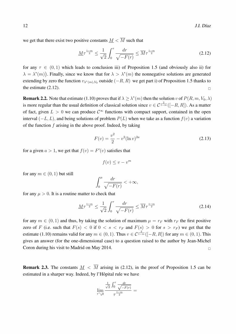
12 J.I. Dıaz
we get that there exist two positive constants M < M such that
Mτ1−m
2 ≤ 1√2
∫ τ
0
dr√−F (r)
≤Mτ1−m
2 (2.12)
for any τ ∈ (0, 1) which leads to conclusion iii) of Proposition 1.5 (and obviously also ii) forλ = λ∗(m)
). Finally, since we know that for λ > λ∗(m) the nonnegative solutions are generated
extending by zero the function vλ∗(m),V0 outside (−R,R) we get part i) of Proposition 1.5 thanks tothe estimate (2.12).
Remark 2.2. Note that estimate (1.10) proves that if λ ≥ λ∗(m) then the solution v of P (R,m, V0, λ)
is more regular than the usual definition of classical solution since v ∈ C2
1−m ([−R,R]). As a matterof fact, given L > 0 we can produce C∞ functions with compact support, contained in the openinterval (−L,L), and being solutions of problem P (L) when we take as a function f(v) a variationof the function f arising in the above proof. Indeed, by taking
F (v) =v2
2− v2(ln v)2a (2.13)
for a given a > 1, we get that f(v) = F ′(v) satisfies that
f(v) ≤ v − vm
for any m ∈ (0, 1) but still ∫ µ
0
dr√−F (r)
< +∞,
for any µ > 0. It is a routine matter to check that
Mτ1−m
2 ≤ 1√2
∫ τ
0
dr√−F (r)
≤Mτ1−m
2 (2.14)
for any m ∈ (0, 1) and thus, by taking the solution of maximum µ = rF with rF the first positivezero of F (i.e. such that F (s) < 0 if 0 < s < rF and F (s) > 0 for s > rF ) we get that theestimate (1.10) remains valid for any m ∈ (0, 1). Thus v ∈ C
21−m ([−R,R]) for any m ∈ (0, 1). This
gives an answer (for the one-dimensional case) to a question raised to the author by Jean-MichelCoron during his visit to Madrid on May 2014.
Remark 2.3. The constants M < M arising in (2.12), in the proof of Proposition 1.5 can beestimated in a sharper way. Indeed, by l’Hopital rule we have
limτ0
1√2
∫ τ0
dr√−F (r)
τ1−m
2
=

Schrodinger infinite potential well 13
Now we are in conditions to prove the main result of this paper:
Proof of Theorem 1. Part 1 holds since if α < 2 thendv
dx(−R) > 0 and
dv
dx(R) < 0. The proof is an
easy adaptation of the Hopf strong maximum principle: see, e.g. [33], [10] and [28].In order to prove Part 2 we shall start by arguing as in the proof of Theorem 3.2 of [24] (see also somefurther results in [22]). For any h ∈ L2(Ω) (Ω = (−R,R)) we define the operator Th = z ∈ H1
0 (Ω)
solution of the linear problem −∆z + V (x)z = h in Ω,z = 0 on ∂Ω.
(2.15)
This operator is well defined since problem (2.15) has a unique (weak) solution z ∈ H10 (Ω). This
follows from applying the Lax-Milgram Lemma to the associated bilinear form in H10 (Ω)
a(u, v) =
∫Ω
∇u · ∇vdx+
∫Ω
V (x)uv dx
which is well-defined, continuous and coercive. Indeed, taking into account that
V (x) ≤ C
d(x, ∂Ω)αa.e. x ∈ Ω,
(thanks to assumption (1.7)) Hardy’s inequality implies that
1
C
∫Ω
V (x)u2dx ≤∫
Ω
u2
d(x)2dx ≤ k
∫Ω
|∇u|2 dx
for some suitable constant k = k(Ω) and then
a(u, u) ≤ C ‖u‖2H1
0 (Ω)
for some C > 0, which implies that a is continuous (the coerciveness of a is a routine matter). Thus,for any h ∈ L2(Ω), there exists a unique Th ∈ H1
0 (Ω) solution of the above equation and it is easyto see that the composition with the (compact) embedding H1
0 (Ω) ⊂ L2(Ω) is a selfadjoint compactlinear operator T = i T : L2(Ω) → L2(Ω) for which we obtain in the usual way a sequence ofeigenvalues νn → +∞. If we call λ# = ν1 then, by well-known results we know that λ# > 0. In
fact, since V (x) ≥ 0, we know that λ# > λ1(R) =( π
2R
)2
.
The proof of Part 3 (i.e. the associated eigenfunctions have zero normal derivatives on the boundary)will result of the application of the iterative method of super and subsolutions (since the comparisonprinciple does not apply directly to solutions of the problem (DP )). We start by proving that if λ#
is the eigenvalue mentioned in Part 2 then we can chose m# ∈ [0, 1) such that
λ# = λ∗(m#) (2.16)
with λ∗(m) the critical eigenvalue of the nonlinear problem P (R,m, V0, λ) given in Proposition 1.5.Indeed, for any m ∈ [0, 1) we have

14 J.I. Dıaz
λ∗(m) =ϕ(m)
2R2
where ϕ(m) :=∫ µ(m)
0dr√
rm+1
m+1− r2
2
, with µ(m) :=(
21+m
) 1(1−m) . Obviously function ϕ(m) is continu-
ous, ϕ(m) > 0 for any m ∈ [0, 1) and
limm1 ϕ(m) = +∞.
Moreover, it is not difficult to check that∫ b
a
dr√r − r2
2
=√
2(arcsin(1− a)− arcsin(1− b)),
and thus
ϕ(0) =
∫ 2
0
dr√r − r2
2
=√
2π.
Then property (2.16) holds since we know that
λ# ≥( π
2R
)2
>
√2π
2R2= λ∗(0).
On the other hand the comparison principle holds, for solutions of the problem
DP (V, f)
−d2u
dx2+ V (x)u = f(x) in Ω,
u = 0 on ∂Ω,
in the sense that, sinceC
d(x, ∂Ω)2≤ V (x), if f, f ∈ H−1(Ω) and f ≤ f in H−1(Ω) then there
exist u, u ∈ H10 (Ω) solutions of DP (V, f) and DP (V, f), respectively, such that u(x) ≤ u(x) a.e.
x ∈ Ω . The proof of this follows by applying again the Hardy inequality (a different argument,when f, f ∈ L1(Ω, δ), can be found in Dıaz and Rakotoson [25]). Then we can apply the iterativemethod of super and subsolutions: we start by building the supersolution of DP (V, λ#,Ω) of theform u(x) = vλ∗(m#)(x : V 0) with vλ∗(m#)(x : V 0) the flat solution of P (R,m#, V 0, λ
∗(m#)).
Thanks to estimates (1.10) and (1.11) and assumption (1.7) for any x ∈ Ω we have
V 0∣∣vλ∗(m#)(x)∣∣1−m# ≤
V 0
(K#)1−m#
1
d(x, ∂Ω)2≤ V (x)
if the conditionV 0
(K#)1−m#≤ C, (2.17)
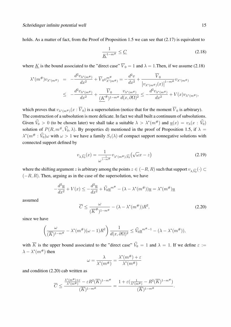
Schrodinger infinite potential well 15
holds. As a matter of fact, from the Proof of Proposition 1.5 we can see that (2.17) is equivalent to
1
K1−m# ≤ C (2.18)
where K is the bound associated to the ”direct case” V 0 = 1 and λ = 1.Then, if we assume (2.18)
λ∗(m#)vλ∗(m#) = −d2vλ∗(m#)
dx2+ V 0v
m#
λ∗(m#) = −d2v
dx2+
V 0∣∣vλ∗(m#)(x)∣∣1−m# vλ∗(m#)
≤ −d2vλ∗(m#)
dx2+
V 0
(K#)1−m#
vλ∗(m#)
d(x, ∂Ω)2≤ −
d2vλ∗(m#)
dx2+ V (x)vλ∗(m#),
which proves that vλ∗(m#)(x : V 0) is a supersolution (notice that for the moment V 0 is arbitrary).The construction of a subsolution is more delicate. In fact we shall built a continuum of subsolutions.Given V0 > 0 (to be chosen later) we shall take a suitable λ > λ∗(m#) and u(x) = vλ(x : V0)
solution of P (R,m#, V0, λ). By properties d) mentioned in the proof of Proposition 1.5, if λ =
λ∗(m# : V0)ω with ω > 1 we have a family S1(λ) of compact support nonnegative solutions withconnected support defined by
vλ,V0(x) =1
ω1
1−m#
vλ∗(m#),V0
(√ωx− z
)(2.19)
where the shifting argument z is arbitrary among the points z ∈ (−R,R) such that support vλ,V0(·) ⊂(−R,R). Then, arguing as in the case of the supersolution, we have
−d2u
dx2+ V (x) ≤ −d
2u
dx2+ V0u
m# − (λ− λ∗(m#))u = λ∗(m#)u
assumedC ≤ ω
(K#
)1−m#− (λ− λ∗(m#))R2, (2.20)
since we have(ω
(K)1−m#− λ∗(m#)(ω − 1)R2
)1
d(x, ∂Ω)2≤ V0u
m#−1 − (λ− λ∗(m#)),
with K is the upper bound associated to the ”direct case” V0 = 1 and λ = 1. If we define ε :=
λ− λ∗(m#) then
ω =λ
λ∗(m#)=λ∗(m#) + ε
λ∗(m#)
and condition (2.20) cab written as
C ≤λ∗(m#)+ελ∗(m#)
− εR2(K)1−m#
(K)1−m#=
1 + ε( 1λ∗(m#)
−R2(K)1−m#)
(K)1−m#.

16 J.I. Dıaz
and this implies that u is a subsolution.Finally, to apply the super and subsolution method we must check
u(x) ≤ u(x) for any x ∈ Ω. (2.21)
From the defintions of u(x) and u(x) we have that (2.21) holds if
V0
λ≤ V 0
λ∗(m#), (2.22)
or equivalently
λ∗(m#) + ε
λ∗(m#)≥ V0
V 0
. (2.23)
Thus we can proceed as follows; we assume
C <1
(K)1−m#. (2.24)
Then, if 1λ∗(m#)
− R2(K)1−m# ≥ 0 then we can take ε > 0 arbitrary and then V 0 and V0 such that
(2.23) holds. If by the contrary 1λ∗(m#)
−R2(K)1−m#< 0 ten we take
ε <1− C(K)1−m#
(R2(K)1−m# − 1λ∗(m#)
)
and again V 0 and V0 such that (2.23) holds.Then, by the super and subsolution method, we get the existence of a minimal u∗(x) and maximalu∗(x) solution of (DP ) such that
u(x) ≤ u∗(x) ≤ u∗(x) ≤ u(x) for any x ∈ Ω.
Since there is a continuum of subsolutions we can shift them in order to get that u∗(x) > 0 for anyx ∈ Ω. Moreover from the spectral theory necessarily Λu∗(x) = u# = Λu∗(x) for some Λ,Λ > 0
and the estimates (1.9) hold for the solutions of the linear problem holds thanks to Proposition 1.5.
Proof of Corollary 1.6. As it is shown in [21], the nodal solutions vλ∗n(m) of the semilinear problemP (R,m, V0, λ) corresponding to suitable values λ∗n(m) of the parameter λ bifurcating at the infinityfrom the simple eigenvalues λn, n ∈ N, are obtained by rescaling, gluing and translating the uniquepositive flat solution corresponding to λ∗(m). Thus the conclusion is an obvious consequence ofProposition 1.5.
Remark 2.4. Theorem 1.2 and Proposition 1.5 also hold to N > 1 for suitable convex regulardomains, for instance, satisfying the interior sphere condition (see [17]).
Schrodinger infinite potential well 17
Proof of Theorem 1.8. Now the comparison principle can be applied directly and so it suffices tofollow the same scheme of proof than in Theorem 1. The sub and supersolutions are obtained bysolving the associate sublinear problem
−∆v + V0vm = f(x) in (−R,R),
v(±R) = 0,
for suitable choices of m ∈ (0, 1) and V0 > 0. The boundary estimate similar to the given in (1.10)was obtained in Theorem 1.15 of [15] (see also [3]) thanks to the crucial assumption (1.12).
Remark 2.5. A different type of localizing results concerning the non-linear Schrodinger equation,arising in nonlinear optics,
i∂ψ
∂t= − 2
2m∆ψ + a|ψ|σψ, in (0,∞)× RN ,
were also presented in the series of lectures [16]. We recall that in most of the papers in the literatureit is assumed σ = 2, nevertheless there are many applications in which σ ∈ (−1, 0). In a series ofpapers in collaboration with P. Begout ([5], [6], [7], [8] and [9]) we prove precise estimates on thelocation of the support of ψ(x, t), whose boundary gives rise to a free boundary associated to theproblem. The techniques of proof are some extensions of the ones of [2] and are entirely differentto the ones used in the present paper.
Remark 2.6. Some of the ideas of this paper can be adapted to the study the existence of ”largesolutions” of the same type of linear equation
−∆u+ V (x)u = f(x) in Ω,u = +∞ on ∂Ω,
when the potential V satisfies (1.7) (see [18]). We recall (Theorem 2.10 of [25]) that given f ∈L1(Ω : δ), f(x) ≥ 0 a.e. x ∈ Ω, V0 > 0, the existence of a large solution of the semilinear problem
−∆v + V0vm = f(x) in Ω,
v = +∞ on ∂Ω,
requires now the key assumption m > 1 (compare this condition to assumption m ∈ (0, 1) used inthe proof of Theorem 1.8 for the existence of a flat solution).
Acknowledgments
The author thanks Th. Cazenave and J. Hernandez for several useful suggestions on a previous ver-sion of this paper. Partially supported by the project ref. MTM2011-26119 of the DGISPI (Spain),

18 J.I. Dıaz
the UCM Research Group MOMAT (Ref. 910480) and the ITN FIRST of the Seventh FrameworkProgram of the European Community’s (grant agreement number 238702).
———restosThen, by Proposition 1.5 and the change of variable (2.8) we know that
0 ≤ u(x) ≤
(V0
λ
) 1
1−m# (2
1 +m#
) 1
(1−m#)
. (2.25)
Then
−d2u
dx2+ V 0u
m# ≤ −d2u
dx2+ V0u
m# − (λ− λ∗(m#))u = λ∗(m#)u
assumedV 0u
m#
+ (λ− λ∗(m#))u ≤ V0um#
. (2.26)
But thanks to the estimate (2.25), the sufficient condition (2.26) holds once we assume
V0(1− (1− λ∗(m#)
λ)(
2
1 +m#)) ≥ V 0. (2.27)
———-restos
References
[1]
[2] ANTONTSEV, S. D IAZ, J. I. AND SHMAREV, S., Energy methods for free boundary problems.Applications to nonlinear PDEs and Fluid Mechanics, Series Progress in Nonlinear Differen-tial Equations and Their Applications, No. 48, Birkauser, Boston, 2002.
[3] ALVAREZ,L. AND D IAZ, J.I. On the retention of the interfaces in some elliptic and parabolicnonlinear problems, Discrete and Continuum Dynamical Systems, 25, (2009), 1-17.
[4] BANDLE, C. AND POZIO, M.A. Sublinear elliptic problems with a Hardy potential. To ap-pear.
[5] BEGOUT, P. AND DIAZ, J.I. On a nonlinear Schrodinger equation with a localizing effect.Comptes Rendus Acad. Sci. Paris, t. 342, Serie I, (2006), 459-463
[6] BEGOUT, P. AND DIAZ, J.I. Localizing Estimates of the Support of Solutions of Some Non-linear Schrodinger Equations: The Stationary Case. Annales de l’Institut Henri Poincare (C)Non Linear Analysis, 29, (2012), 35-58

Schrodinger infinite potential well 19
[7] BEGOUT, P. AND DIAZ, J.I. A sharper energy method for the localization of the support tosome stationary Schrodinger equations with a singular nonlinearity. Discrete and ContinuousDynamical System Series A, 34 (9) (2014), 3371-3382.
[8] BEGOUT, P. AND DIAZ, J.I. Self-similar solutions with compactly supported profile of somenonlinear Schrodinger equations. Electronic Journal Differential Equations. vol 2014 (2014),No. 90, 1-15.
[9] BEGOUT, P. AND DIAZ, J.I. Existence of weak solutions to some stationary Schrodingerequations with singular nonlinearity. Rev. R. Acad. Cien. Serie A. Mat. (RACSAM). To appear.
[10] BERSCH, M. AND ROSTAMIAN, R. The principle of linearized stability for a class of degen-erate diffusion equations. J. Differ. Equat, 57, (1985) 373–405.
[11] BENILAN, PH., BREZIS, H. AND M.G. CRANDALL, M.G. A semilinear equation in L1(RN ),Ann. Scuola Norm. Sup. Pisa 4, 2 (1975), 523–555.
[12] BREZIS, H. Solutions of variational inequalities with compact support. Uspekhi Mat. Nauk.,129, (1974) 103-108.
[13] BREZIS, H. AND STAMPACCHIA, G. Une nouvelle methode pour l’etude d’ecoulements sta-tionnaires,C.R. Acad. Sci., 276, 1973, 129-132.
[14] BREZIS, H. AND STAMPACCHIA, G. The hodograph method in Fluid-Dynamics in the lightof Variational Inequalities, Arch. Rat. Mech.Anal., 61, (1976), 1-18.
[15] D IAZ, J.I. Nonlinear Partial Differential Equations and Free Boundaries. Research Notes inMathematics, 106, Pitman, London 1985.
[16] D IAZ, J.I. Lectures on the Schrodinger equation for the ”infinite well potential. In the booksof abstracts of the congresses Quasilinear PDEs, Tours (France), June 4-6, 2012; NonlinearPartial Differential Equations, Valencia (Spain) July 1-5, 2013; Free Boundary Problems Pro-gramme”of the Newton Institute (January-July 2014), Cambridge (UK), May 22, 2014.
[17] D IAZ, J.I. On the ambiguous treatment of the Schrodinger equation for infinite potential welland an alternative via flat solutions: the multi-dimensional case. To appear.
[18] D IAZ, J.I. On the existence of large solutions for linear elliptic equations with a Hardy ab-sorption potential. To appear.
[19] D IAZ, J.I. AND HERNANDEZ, J. Global bifurcation and continua of nonnegative solutions fora quasilinear elliptic problem, Comptes Rendus Acad. Sci. Paris, 329, Serie I, (1999), 587-592.

20 J.I. Dıaz
[20] D IAZ, J.I. AND HERNANDEZ. J. On a countable set of branches bifurcating from theinfinity of nodal solutions for a singular semilinear equation. Proc. of the 5th Inter-national Conference on Approximation Methods and Numerical Modelling in Environ-ment and Natural Resources, MAMERN13, .B. Amaziane et al. eds., Editorial Universi-dad de Granada, Granada, Spain, 2013, p. 118 (see also the extended abstract version athttps://www.ugr.es/˜mamern/mamern13)
[21] D IAZ, J.I. AND HERNANDEZ, J. Positive and nodal solutions bifurcating from the infinity fora semilinear equation: solutions with compact support. To appear.
[22] D IAZ, J.I., HERNANDEZ, J. AND MAAGLI, H., to appear.
[23] D IAZ, J.I., HERNANDEZ, J, AND F.J. MANCEBO, F.J. Branches of positive and free bound-ary solutions for some singular quasilinear elliptic problems. J. Math. Anal. Appl. 352 (2009)449–474).
[24] D IAZ, J.I., HERNANDEZ, J. AND Y ILYASOV, Y. On the existence of positive solutions andsolutions with compact support for a spectral nonlinear elliptic problem with strong absorption.To appear in Nonlinear Analysis Series A: Theory, Mehods and Applications.
[25] D IAZ, J.I. AND RAKOTOSON, J.-M., On very weak solutions of semilinear elliptic equationswith right hand side data integrable with respect to the distance to the boundary, Discrete andContinuum Dynamical Systems, 27, (2010), 1037-1058.
[26] GALINDO, A. AND PASCUAL, P. Quantum Mechanics I, Springer-Verlag, Berlin, 1990.
[27] GAMOW, G., Zur Quantentheorie des Atomkernes, Zeitschrift fur Physik 51, 204 (1928), 204-212.
[28] HERNANDEZ,J., MANCEBO,F.J. AND VEGA, J.M. On the linearization of some singularnonlinear elliptic problems and applications, Ann. Inst. H. Poincare Anal., 19 (2002), 777-813.
[29] JOGLEKAR, Y.N. Particle in a box with a -function potential: Strong and weak coupling limits,Am. J. Phys. 77, (2009), 734–736.
[30] KAPER,H. AND KWONG,M., Free boundary problems for Emden-Fowler equation, Differen-tial and Integral Equations, 3, (1990), 353-362.
[31] LEIGHTON, R. B., Principles of Modern Physics-McGraw-Hill Inc., New York, 1959.
[32] NAIMARK, M.A. Linear Differential Operators, Ungr, New York, 1968.
Schrodinger infinite potential well 21
[33] PROTTER, M.H. AND WEIMBERGER, H.F., Maximum Principles in Differential Equations.New York, Springer-Verlag, 1984.
[34] PUCCI, P. AND SERRIN, J. The maximum principle, Progress in Nonlinear Differential Equa-tions and Their Applications, 73, Birkhauser Verlag, Basel, 2007.
[35] STRAUSS, W., Partial Differential Equations. An Introduction, John Wiley and Sons, NewYork, 1992.
[36] VAZQUEZ, J.V. A strong maximum principle for some quasilinear elliptic equations, Appl.Math. Optim. 12, (1984), 191-202.
Related Documents


