On Systematic Scan Thesis submitted in accordance with the requirements of the University of Liverpool for the degree of Doctor in Philosophy by Kasper Pedersen. First Supervisor: Prof. Leslie Ann Goldberg Second Supervisor: Dr. Paul W. Goldberg Department of Computer Science The University of Liverpool January, 2008

Welcome message from author
This document is posted to help you gain knowledge. Please leave a comment to let me know what you think about it! Share it to your friends and learn new things together.
Transcript

On Systematic Scan
Thesis submitted in accordance with therequirements of the University of Liverpoolfor the degree of Doctor in Philosophy by
Kasper Pedersen.
First Supervisor: Prof. Leslie Ann GoldbergSecond Supervisor: Dr. Paul W. Goldberg
Department of Computer ScienceThe University of Liverpool
January, 2008


Preface
This thesis is predominantly my own work and the sources from which material
is drawn are identified within. This is a brief summary of these.
Chapters 1 and 2 contain introductory material and a literature survey draw-
ing from the works of several different authors. Furthermore Chapter 2 contains
definitions used throughout this thesis, some of which are taken from Weitz [55].
Chapter 3 is based on a paper [47] published in MFCS 2007. The bibliograph-
ical details of the paper are:
• Kasper Pedersen. Dobrushin conditions for systematic scan with block dy-
namics. In Ludek Kucera and Antonın Kucera, editors, MFCS, volume 4708
of Lecture Notes in Computer Science, pages 264–275. Springer, Berlin,
2007.
Chapter 3 furthermore contains two proofs of theorems by Weitz which are out-
lined in Weitz [55].
Chapter 4 is based on a paper [48] submitted for publication. The biblio-
graphical details of the paper are:
• Kasper Pedersen. On systematic scan for sampling H-colourings of the
path. arXiv:0706.3794 (submitted), 2007.
Chapter 5 is based on a paper [38] submitted for publication. The paper is
joint work with Markus Jalseniuis and both authors made equal contributions to
the preparation of that paper. The bibliographical details of the paper are:
• Markus Jalsenius and Kasper Pedersen. A systematic scan for 7-colourings
of the grid. arXiv:0704.1625 (submitted), 2007.


Abstract
In this thesis we study the mixing time of systematic scan Markov chains on
finite spin systems. A systematic scan Markov chain is a Markov chain which
updates the sites in a deterministic order and this type of Markov chain is often
seen as intuitively appealing in terms of implementation to scientists conducting
experimental work. Until recently systematic scan Markov chains have largely
resisted analysis and a gap in the parameters that imply rapid mixing has de-
veloped between systematic scan Markov chains and the more frequently studied
random update Markov chains. We reduce this gap in this thesis by improving the
parameters for which systematic scan mixes when applied to several well-known
spin systems.
The main contribution of this thesis is the introduction of a new technique
for proving rapid mixing of systematic scan Markov chains. It is known that,
in a single-site setting, the mixing time of systematic scan can be bounded in
terms of the influence that sites have on each other. We generalise this technique
for bounding the mixing time of systematic scan to block dynamics, a setting in
which a (constant size) set of sites are updated simultaneously. In particular we
introduce a parameter corresponding to the maximum influence on any site and
show that if this parameter is sufficiently small, then the corresponding systematic
scan Markov chain mixes rapidly.
We present several applications of this new proof technique. In particular
we show that systematic scan mixes rapidly on spin systems corresponding to
proper q-colourings of (1) general graphs, (2) trees, and (3) the grid for improved
parameters than were previously known. We also obtain rapid mixing of sys-
tematic scan Markov chains for sampling H-colourings of the n-vertex path for a
restricted family of H using this technique. The H-colouring result is extended
to general graphs H by placing more restrictions on the scan and using path cou-
pling, a well-established technique for bounding mixing times of Markov chains.
Path coupling is also used to prove rapid mixing of a single-site systematic scan
for sampling proper q-colourings of bipartite graphs.


Acknowledgements
I would like to extend a particular debt of gratitude to my main supervisor Leslie
Ann Goldberg who has been an excellent supervisor both as a graduate and
undergraduate student. In my research I have befitted immensely from Leslie’s
technical insights, attention to detail and ability to explain ideas and concepts in a
clear and understandable fashion. Leslie has provided me with countless detailed
and useful suggestions for ways to improve drafts of the papers that form the
basis of this thesis. Furthermore, her friendly and enthusiastic personality has
helped to make my time as a PhD student highly enjoyable.
I would also like to thank my second supervisor whilst at Liverpool University,
Paul Goldberg, for useful conversations and suggestions.
I am grateful to both of my examiners, Mark Jerrum and Russell Martin, for
the time and effort they put into examining this thesis and for several very helpful
comments and suggestions for improvement during my viva.
I have been fortunate to have been part of two very good research groups
during my time as a PhD student. For that I would like to thank the members
of the Algorithms and Complexity research group at Warwick University and
the members of the Complexity Theory and Algorithmics Group at Liverpool
University. Both of these groups have formed an excellent environment in which to
conduct research. Special thanks go to my officemates and good friends: Markus
Jalsenius (with whom I had the pleasure of coauthoring a paper), Nick Palmer
and Pattarawit Polpinit (A).
Last, but by no means least, I would like to thank my family and friends,
especially my wife, my parents and my brother, for their support throughout my
entire academic career.
Kasper Pedersen

Contents
Notation Glossary ix
1 Introduction 1
1.1 Summary of Results . . . . . . . . . . . . . . . . . . . . . . . . . 10
1.2 Plan of Thesis and Biographical Notes . . . . . . . . . . . . . . . 11
2 Preliminaries 13
2.1 Spin Systems . . . . . . . . . . . . . . . . . . . . . . . . . . . . . 13
2.2 Markov Chains and Mixing Time . . . . . . . . . . . . . . . . . . 16
2.3 Coupling and Path Coupling . . . . . . . . . . . . . . . . . . . . . 18
2.4 Block Dynamics and Influence Parameters . . . . . . . . . . . . . 26
2.5 Statement of Results . . . . . . . . . . . . . . . . . . . . . . . . . 29
2.5.1 A Dobrushin Condition for Rapid Mixing of SystematicScan with Block Dynamics . . . . . . . . . . . . . . . . . . 29
2.5.2 Sampling H-colourings of the Path . . . . . . . . . . . . . 33
2.5.3 Sampling 7-colourings of the Grid . . . . . . . . . . . . . . 36
2.5.4 Single-site Systematic Scan for Bipartite Graphs . . . . . . 37
3 A Dobrushin Condition for Systematic Scan with Block Dynam-ics 39
3.1 Preliminaries . . . . . . . . . . . . . . . . . . . . . . . . . . . . . 40
3.2 Bounding the Mixing Time of Systematic Scan . . . . . . . . . . 43
3.3 Application: Edge Scan on an Arbitrary Graph . . . . . . . . . . 48
3.3.1 Overview of the Coupling . . . . . . . . . . . . . . . . . . 49
3.3.2 Details of Coupling and Proof of Mixing . . . . . . . . . . 51
3.4 Application: Colouring a Tree . . . . . . . . . . . . . . . . . . . . 68
3.4.1 A Single-site Systematic Scan . . . . . . . . . . . . . . . . 69
3.4.2 A Systematic Scan with Block Dynamics . . . . . . . . . 71
3.5 A Comparison of Influence Parameters . . . . . . . . . . . . . . . 80
4 Sampling H-colourings of the n-vertex Path 90
4.1 Preliminaries . . . . . . . . . . . . . . . . . . . . . . . . . . . . . 90
4.2 H-colourings of the Path for a Restricted Family of H . . . . . . . 95
4.3 H-colourings of the Path for any H . . . . . . . . . . . . . . . . . 102
4.4 H-colourings of the Path with a Random Update Markov Chain . 112
iv

Contents v
5 Sampling 7-colourings of the Grid 1145.1 Preliminaries . . . . . . . . . . . . . . . . . . . . . . . . . . . . . 1145.2 Bounding the Mixing Time of Systematic Scan . . . . . . . . . . . 1165.3 Constructing the Coupling by Machine . . . . . . . . . . . . . . . 120
5.3.1 Representing a Coupling as a Bipartite Graph . . . . . . . 1205.3.2 Proof of Lemma 71 . . . . . . . . . . . . . . . . . . . . . . 121
5.4 Partial Results for 6-colourings of the Grid . . . . . . . . . . . . 1235.4.1 Establishing Lower Bounds for 2×2 Blocks . . . . . . . . . 1245.4.2 Bigger Blocks . . . . . . . . . . . . . . . . . . . . . . . . . 125
6 Single-site Systematic Scan for Bipartite Graphs 1296.1 Preliminaries . . . . . . . . . . . . . . . . . . . . . . . . . . . . . 1296.2 Definition of the Coupling . . . . . . . . . . . . . . . . . . . . . . 1306.3 Proof of Mixing . . . . . . . . . . . . . . . . . . . . . . . . . . . . 132
7 Conclusion 141
Bibliography 145

List of Figures
2.1 The graph describing the independent sets model. Sites assignedcolour 0 are “unoccupied’ and sites assigned 1 are “occupied”. . . 15
2.2 The graph describing the Beach model. . . . . . . . . . . . . . . . 15
2.3 The graph describing the 4-particle Widom-Rowlinson model. . . 15
3.1 Case 1. Exactly one site in Θk is adjacent to i. Let this site belabeled j and let the other site in Θk be labeled j′. . . . . . . . . 50
3.2 Case 2. Both sites in Θk are adjacent to i and no other sites in∂Θk are coloured 1 or 2. The labeling of the sites in Θk is arbitrary. 50
3.3 Case 3. Both sites in Θk are adjacent to i. One of the sites in Θk
is adjacent to at least one site, other than i, coloured 1 (or 2). Letthis site be labeled j′. The other site in Θk is labeled j and it isnot adjacent to any site, other than i, coloured 1 or 2. . . . . . . . 50
3.4 Case 4. Both sites in Θk are adjacent to i. One of the sites in Θk isadjacent to at least one site, other than i, coloured 1 and no sitesthat are coloured 2. Let this site be labeled j′. The other site inΘk, labeled j, is adjacent to at least one site other than i coloured2 and no sites coloured 1. . . . . . . . . . . . . . . . . . . . . . . . 51
3.5 Case 5. Both sites in Θk are adjacent to i and at least one site,other than i coloured 1 (or 2). The labeling of the sites in Θk isarbitrary. . . . . . . . . . . . . . . . . . . . . . . . . . . . . . . . 51
3.6 Case 1 (repeat of Figure 3.1). Exactly one site in Θk is adjacent toi. Let this site be labeled j and let the other site in Θk be labeled j′. 52
3.7 Case 2 (repeat of Figure 3.2). Both sites in Θk are adjacent to iand no other sites in ∂Θk are coloured 1 or 2. The labeling of thesites in Θk is arbitrary. . . . . . . . . . . . . . . . . . . . . . . . . 55
3.8 Case 3 (repeat of Figure 3.3). Both sites in Θk are adjacent to i.One of the sites in Θk is adjacent to at least one site, other thani, coloured 1 (or 2). Let this site be labeled j′. The other site inΘk is labeled j and it is not adjacent to any site, other than i,coloured 1 or 2. . . . . . . . . . . . . . . . . . . . . . . . . . . . . 57
3.9 The pair of configurations after the colour of site j′ has been as-signed during the first step of the coupling. . . . . . . . . . . . . . 59
vi

List of Figures vii
3.10 Case 4 (repeat of Figure 3.4). Both sites in Θk are adjacent to i.One of the sites in Θk is adjacent to at least one site, other than i,coloured 1 and no sites that are coloured 2. Let this site be labeledj′. The other site in Θk, labeled j, is adjacent to at least one siteother than i coloured 2 and no sites coloured 1. . . . . . . . . . . 60
3.11 Case 5 (repeat of Figure 3.5). Both sites in Θk are adjacent to iand at least one site, other than i coloured 1 (or 2). The labelingof the sites in Θk is arbitrary. . . . . . . . . . . . . . . . . . . . . 62
3.12 The region defined in a boundary pair and the construction of thesubtrees. . . . . . . . . . . . . . . . . . . . . . . . . . . . . . . . 73
3.13 A block in the tree. A solid line indicates an edge and a dottedline the existence of a path. . . . . . . . . . . . . . . . . . . . . . 76
3.14 The influence on site j via the root. A line denotes an edge and adotted line the existence of a simple path. . . . . . . . . . . . . . 79
4.1 A block Θk of length l1. . . . . . . . . . . . . . . . . . . . . . . . 1004.2 Site i is on the boundary of Θa and is not contained in any block
Θa′ with a′ < a. . . . . . . . . . . . . . . . . . . . . . . . . . . . . 110
5.1 General labeling of the sites in a 2×2-block Θk and the sites ∂Θk
on the boundary of the block. . . . . . . . . . . . . . . . . . . . . 1175.2 A 2×2-block Θk showing all eight positions of a site i ∈ ∂Θk on
the boundary of the block in relation to a site j ∈ Θk in the block. 1185.3 (a) General labeling of the sites in a 2×3-block Θk and the sites
∂Θk on the boundary of the block. (b)–(c) All ten positions ofa site i ∈ ∂Θk on the boundary of the block in relation to a sitej ∈ Θk in the corner of the block. . . . . . . . . . . . . . . . . . . 126
5.4 (a)–(b) General labeling of the sites in a 3×3-block Θk and twodifferent labellings of the sites ∂Θk on the boundary of the block.The discrepancy site on the boundary has label z1. (b)–(c) Alltwelve positions of a site i ∈ ∂Θk on the boundary of the block inrelation to a site j ∈ Θk in the corner of the block. . . . . . . . . 127

List of Tables
2.1 Optimising the number of colours using blocks . . . . . . . . . . . 32
3.1 Optimising the number of colours using blocks . . . . . . . . . . . 42
viii

Notation Glossary
Basic Notation
Z The set of integers.
N The set of positive integers including zero.
R The set of real numbers.
R≥0 The set of positive real numbers including zero.
1a=b Indicator function taking value 1 if a = b and value 0 otherwise.
Spin Systems and Markov Chains
V The set of sites (V = 1, . . . , n).C The set of spins (C = 1, . . . , q).Ω+ The set of all configurations of a spin system (Ω+ = CV ).
π The Boltzmann distribution of a spin system.
Ω The set of legal configurations; configurations with positive measure
in π.
xi The spin assigned to site i under some configuration x ∈ Ω+.
Si A pair of configurations differing only on the spin assigned to site i.
dTV(·, ·) The total variation distance between two probability distributions.
MRU A random update Markov chain. A random update Markov chain
makes a transition by randomly selecting a subset of sites (from
some specified set of subsets of V ) and updating the spins assigned
to the sites in the selected subset.
M→ A systematic scan Markov chain. A systematic scan Markov chain
makes a transition updating the subsets of sites (for some specified
set of subsets of V ) one at the time in a deterministic order.
ix

x Notation Glossary
Block Dynamics and Influence Parameters
Θk A block with index k; Θk ⊆ V .
Θ covers V A set of blocks Θ covers the set of sites V if⋃
k Θk = V .
∂Θk The set of sites adjacent to Θk; ∂Θk is the boundary of Θk.
x = y off Θk The configurations x and y are assigned the same spin on
all sites in V \Θk.
x = y on Θk The configurations x and y are assigned the same spin on
all sites in Θk.
P [k] The transition matrix for updating block Θk.
P [k](x, ·) The distribution on configurations resulting from
applying P [k] to a configuration x.
Ψk(x, y) A coupling of the distributions P [k](x, ·) and P [k](y, ·).(x′, y′) ∈ Ψk(x, y) A pair of configurations (x′, y′) drawn from Ψk(x, y).
ρki,j The influence of site i on site j under the update of block
Θk; ρki,j = max(x,y)∈Si
Pr(x′,y′)∈Ψk(x,y)x′j 6= y′j.
α The maximum influence on any site in the graph;
α = maxk maxj∈Θk
∑i∈V ρk
i,jwi/wj where wi is a positive
weight assigned to site i for each i ∈ V .

Chapter 1
Introduction
This thesis is concerned with the study of finite spin systems. A finite spin sys-
tem is composed of a set of sites and a set of spins, both of which are finite.
The sites are vertices of an underlying graph whose edges specify the intercon-
nection between the sites. The underlying graph is assumed to be connected. A
configuration of the spin system is an assignment of a spin to each site. If there
are n sites and q available spins then this gives rise to qn possible configurations,
however some configurations may be illegal depending on the specification of the
spin system. The specification of the system determines how spins interact with
each other at a local level, such that different local configurations on a subset
of the graph may have different relative likelihoods. In particular, for spin sys-
tems with so-called hard-constraints the specification states which pairs of spins
are permitted to be assigned to adjacent sites and which pairs of spins are not.
This interaction between sites specifies a well-defined probability distribution π
(known as the Boltzmann distribution) on the set of all configurations of a spin
system. Configurations with positive measure in π are said to be legal.
Many models, often originating from the field of statistical physics, fall under
the general category of spin systems. As a simple, but important, example con-
sider a spin system in which no two adjacent sites are permitted to be assigned
the same spin. This spin system corresponds to the q-state anti-ferromagnetic
Potts model at zero temperature, a frequently studied model in statistical me-
chanics. This spin system is also well-known in the field of theoretical computer
science where a legal configuration of the system is commonly known as a proper
q-colouring of the underlying graph. Several of the results presented in this thesis
will be for this spin system, and when discussing proper q-colourings it is natural
to refer to the spins as colours.
Another well-known example of a spin system is the independent sets model.
1

2 1: Introduction
In the independent sets model each site is either “occupied” or “unoccupied” and
in a legal configuration no two adjacent sites are allowed to be occupied. It is usual
to assign a positive weight λ to each occupied site, and in this weighted setting
the spin system is known as the hard-core lattice gas model. This spin system has
been used as a model of gas in the field of statistical physics (Georgii [30] cited in
Weitz [54]) and has also been used in the modeling of communication networks
by Kelly [42].
A natural formalisation of spin systems with hard constraints is the H-colouring
model. An H-colouring of a graph G is a homomorphism from G to some fixed
graph H. The vertices of H correspond to spins and the edges of H specify which
spins are allowed to be adjacent in an H-colouring of G. The H-colouring model
is a natural generalisation of the proper colouring model since if H is the q-clique
then an H-colouring of a graph is a proper colouring. H-colouring problems have
attracted much interest from computer scientists and combinatorialists alike and
much progress has been made. In fact, Hell and Nesetril [37] gave a complete char-
acterisation of graphs H for which the decision problem of determining whether
a given graph has an H-colouring for a specific H is NP-complete. They showed
that if H has a loop or is bipartite then the problem is in P, and that the problem
is NP-complete for any other fixed H. A complete dichotomy is also known for the
problem of counting the number of H-colourings of a given graph. This counting
problem is of natural interest to combinatorialists, and we will be interested in
studying problems closely related to counting in this thesis. This dichotomy is
due to Dyer and Greenhill [24] who showed that if H has at least one nontrivial
component then the counting problem is complete for the complexity class #P.
Otherwise it is in P. A trivial component is a connected component which is either
a complete graph with all loops present, or a complete bipartite graph with no
loops present. The complexity class #P was introduced by Valiant [52] in 1979
and it contains enumeration problems. For a more detailed description of this
complexity class see Jerrum [40]. Dyer and Greenhill furthermore showed that
the same dichotomy holds even when the underlying graph is of bounded degree.
This is an interesting observation since in many physical applications the under-
lying graph tends to be of low degree. Interestingly the above characterisation
for the decision problem does not hold for bounded degree graphs as was shown
by Galluccio, Hell and Nesetril [29]. Despite the hardness of exactly counting the
number of H-colourings of a graph, it remains possible to approximately count
the number of H-colourings as we will discuss subsequently.
For a given spin system it is of interest to sample from the probability distri-

3
bution π, especially when π is uniform over the set of legal configurations Ω of
the spin system. In statistical physics this interest is due to the connection that
π has with various equilibrium properties of a spin system. In theoretical com-
puter science much of the reason for interest in the sampling problem is the, now
well-established, connection between (nearly) uniform sampling and approximate
counting established by Jerrum, Valiant and Vazirani [41]. They showed that the
(nearly) uniform sampling problem and the approximate counting problems are
equally hard for a subclass of counting problems which satisfy a property called
self-reducibility. This subclass contains many interesting instances of counting
problems, notably proper q-colourings. Specifically, the problem of uniform sam-
pling reduces to the problem of approximately counting the number of elements
in Ω and vice versa for all self-reducible counting problems. For an exposition
account of these developments see for example the book by Jerrum [40] or the sur-
vey paper by Dyer and Greenhill [23]. Both of these publications focus on some
of the most well-studied models in computer science, such as proper q-colourings
and independent sets, and many papers concerned with studying techniques for
sampling proper colourings or independent sets have been motivated by this ex-
plicit connection between sampling and counting. The first counting-to-sampling
reduction applicable to general H-colourings was due to Dyer, Goldberg and Jer-
rum [17] although currently no completely general sampling-to-counting reduction
is known. Hence, if there exists a polynomial time (in the number of sites of the
underlying graph) algorithm for sampling from the (near) uniform distribution
of H-colourings of a graph then there also exists a polynomial time algorithm
for approximately counting the number of H-colourings of that graph. With this
result in mind we will focus on the problem of sampling from π for a given spin
system.
Given a spin system, the problem of sampling from π is a challenging task.
Goldberg, Kelk and Paterson [32] studied the complexity of this sampling prob-
lem for H-colourings in the case when π is uniform over Ω and showed that
if H has no nontrivial components then the sampling problem is intractable in
a complexity-theoretic sense. That is, they prove that there is unlikely to be
any algorithm that can efficiently obtain a sample from π (this is known as a
Polynomial Almost Uniform Sampler) by reducing the problem of approximately
counting independent sets in bipartite graphs, which in turn is complete with
respect to approximation preserving reductions for a logically-defined subclass of
#P (see Dyer, Goldberg, Greenhill and Jerrum [15] for results about this com-
plexity class), to the problem of sampling from the (near) uniform distribution of
4 1: Introduction
H-colourings. This does, however, not rule out the possibility of sampling from
the uniform distribution of general H-colourings of more restricted graphs G.
As the task of sampling from π is computationally difficult it is often the
case that the only feasible method of carrying out this task is by simulating
some suitable random dynamics converging to π. Ensuring that such a dynamics
converges to π is generally straightforward, but obtaining good upper bounds on
the number of steps required for the dynamics to become sufficiently close to π
is a much more difficult problem. One of the most common type of dynamics
used is a Markov chain. A Markov chain is a stochastic process whose states
(in our case) are the set of configurations of the given spin system with positive
measure in π. By construction of the Markov chain it is generally straightforward
to ensure that it converges to π, however providing good upper bounds on the rate
of convergence, known as the mixing time of the Markov chain, is a much more
difficult task. For this sampling method to be feasible we need to ensure that the
Markov chain converges to π in a polynomial number of steps. Due to a lack of
theoretical convergence results, scientists conducting experiments by simulating
such dynamics are at times forced to “guess” (using some heuristic methods)
the number of steps required for their dynamics to be sufficiently close to the
desired distribution. Cowles and Carlin [9] give a comprehensive review of some
diagnostic tools used to empirically determine these convergence rates and include
some examples from applications in the field of bio-statistics. One immediate
problem, which is pointed out by Cowles and Carlin, with many convergence
diagnostics is that they might prematurely claim convergence of the dynamics
and another is that by continuously monitoring the dynamics one may implicitly
introduce a conditioning that can in turn create a bias in the sampling procedure
(see Cowles, Roberts and Rosenthal [10]). The negative effect these and other
issues have on the effectiveness of practical applications can be greatly reduced
using more sophisticated diagnostic tools, however the existence of good analytical
bounds on the convergence rates would eliminate the need for such techniques to
be employed in the first place. By establishing rigorous bounds on the mixing
time of these Markov chains, computer scientists can provide underpinnings for
this type of experimental work and also allow a more structured approach to be
taken.
Analysing the mixing time of Markov chains for sampling from π for various
spin systems is a well-studied area in theoretical computer science and as a result
of this interest there is a substantial body of literature concerned with inventing
Markov chains for sampling from π and providing upper bounds on their mixing

5
times. We now briefly survey some of the contributions made. When the spin
system corresponds to proper q-colourings of a graph with maximum vertex-
degree ∆ and π is uniform over the set of proper colourings then Jerrum [39], and
independently Salas and Sokal [50], showed that a simple Markov chain mixes
in O(n log n) updates when q > 2∆. This Markov chain makes transitions by
selecting a site v and a colour1 c uniformly at random, and then recolouring site
v to c if doing so results in a proper q-colouring of the graph. By considering a
more complicated Markov chain Vigoda [53] was able to weaken the restriction
on q to q > (11/6)∆ being sufficient for proving mixing in O(n log n) updates.
This remains the least number of colours required for rapid mixing of a Markov
chain for uniformly sampling q-colourings of general graphs, however the number
of colours can be further reduced for restricted families of graphs. For example, in
the important case when the underlying graph is the grid then Goldberg, Martin
and Paterson [33] gave a hand-proof that q = 7 colours are sufficient for mixing
in O(n log n) updates by establishing a condition called “strong spatial mixing”
which in turn implies rapid mixing (see Dyer, Sinclair, Vigoda and Weitz [26]).
Achlioptas, Molloy, Moore and van Bussel [1] further showed that q = 6 colours
are sufficient for a Markov chain for proper colourings of the grid to mix in
O(n log n) updates using a computer-assisted proof. As a final example for proper
q-colourings Martinelli, Sinclair and Weitz [46] showed that q = ∆+2 colours are
sufficient for O(n log n) mixing when the underlying graph is a tree, improving a
related result by Kenyon, Mossel and Peres [43].
When the spin system corresponds to independent set configurations with pa-
rameter λ then the condition λ < 2∆−2
is sufficient for O(n log n) mixing as shown
by Dyer and Greenhill [25] and independently Luby and Vigoda [45] (although
the latter result is restricted to triangle-free graphs). When ∆ ≤ 4 these results
include the λ = 1 case which is of special interest to computer scientists since it
corresponds to sampling from the uniform distribution on independent sets of the
graph. Weitz [56] has recently given a completely different algorithm, namely a
deterministic algorithm with polynomial running time, which improves the con-
dition on λ to λ < (∆−1)∆−1/(∆−2)∆. This notably includes the λ = 1 case for
∆ = 5. An interesting aspect of work carried out on the independent sets model
is that, as well as the aforementioned positive results regarding the mixing times
of various Markov chains, a number of negative results are known as we will now
discuss. When ∆ ≥ 6 and λ = 1 then Dyer, Frieze and Jerrum [14] have shown
1Recall that we use the term colour rather than spin when discussing spin systems corre-sponding to proper colourings.

6 1: Introduction
that there exists a bipartite graph G0 such that any so-called cautious Markov
chain on independent set configurations of G0 has (at least) exponential mixing
time (in the number of sites of G0). A Markov chain is said to be cautious if it is
only allowed to change the state of a constant fraction of sites at the time. This
negative result was generalised to H-colourings by Cooper, Dyer and Frieze [8].
Their result applies to graphs H that are either bipartite or have at least one
loop present, and is not a complete graph with all loops present (observe that for
such an H the decision problem is in P and the counting problem is in #P as
discussed above). In particular this result guarantees the existence of a ∆-regular
graph G0 (with ∆ depending on H) such that any cautious Markov chain on the
set of H-colourings of G0, and with uniform stationary distribution, has a mixing
time that is at least exponential in the number of sites of G0.
While much is understood about the mixing times of Markov chains for sam-
pling from π, the types of Markov chains frequently studied by computer scientists
do not always correspond to the types of dynamics used in experimental work.
Most of the Markov chains previously studied make transitions by randomly se-
lecting a set of sites (often just a single site) and updating the spins assigned to
those sites according to some well-defined distribution induced by π. We call this
type of chain a random update Markov chain and point out that all the positive
results described above are for random update Markov chains. The mixing time
of a random update Markov chain is measured in the number of updates required
in order for the Markov chain to mix. An alternative to random update Markov
chains is to construct a Markov chain that cycles through and updates the sites
(or subsets of sites) in a deterministic order. We call this a systematic scan
Markov chain (or systematic scan for short). The mixing time of a systematic
scan Markov chain is measured in the number of scans of the graph required to
mix and throughout this thesis it holds that one scan of the graph takes O(n)
updates. It is important to note that systematic scan remains a random process
since the method used to update the colour assigned to the selected set of sites
is a randomised procedure drawing from some well-defined distribution induced
by π. Systematic scan may be more intuitively appealing that random update
Markov chains in terms of implementation, however until recently this type of
dynamics has largely resisted analysis when applied to spins systems with hard
constraints. Dynamics that make deterministic choices about about the order in
which sites are updated have however been used in practical applications. In a
study of the effect the rules for selecting sites for update has on the convergence
rates Fishman [27] outlined five plans for selecting the update order, three of

7
which were deterministic rules, as well as giving some practical comparisons. A
practical comparison is also given by Roberts and Sahu [49] for the problem of
sampling from a Gaussian distribution with applications in image analysis. They
showed that for two classes of sampling problems a deterministic strategy is bet-
ter than a random update strategy. However they also gave examples of instances
from outside those classes where random update performs better. An example
that is more combinatorial in nature and as such is closer to the applications we
will consider in this thesis is Diaconis and Ram [11] who studied systematic scan
in the context of generating random elements of a finite group and successfully
bounded the number of scans required to mix. This thesis is concerned with
studying the problem of sampling from π for any given spin system by simulating
systematic scan Markov chains, and especially with bounding the mixing times
of these chains.
Only few results providing bounds on the mixing time of systematic scan
Markov chains for sampling from π exist in the literature and almost all of them
focus on proper q-colourings of bounded degree graphs. For general graphs, sys-
tematic scan is known to mix in O(log n) scans whenever q > 2∆ where ∆ is
the maximum vertex-degree of the graph. This result is obtained by studying
the influences that the sites have on each other and is due to Dyer, Goldberg
and Jerrum [18]. This approach also gives a mixing time of O(n2) scans in the
q = 2∆ case. In Chapter 3 we improve the mixing time of systematic scan for
general graphs in the q = 2∆ case to O(log n) scans. If the underlying graph
is bipartite then a systematic scan mixes in O(log n) scans whenever q > f(∆)
where f(∆) → β∆ as ∆ →∞ and β ≈ 1.76. This result is obtained by a careful
construction of the metric used in the path coupling construction and is due to
Bordewich, Dyer and Karpinski [4]. When considering tree graphs, it is known
that systematic scan mixes in O(log n) scans whenever q > ∆ + 2√
∆− 1 and in
O(n2 log n) scans whenever q = ∆ + 2√
∆− 1 is an integer; see e.g. Hayes [36]
or Dyer, Goldberg and Jerrum [19]. In Chapter 3 we will further reduce the
number of colours required to prove rapid mixing for systematic scan on trees.
Furthermore, Dyer, Goldberg and Jerrum [20] have shown that a systematic scan
for proper 3-colourings of the n-vertex path mixes in Θ(n2 log n) scans when con-
sidering a systematic scan that updates one site at the time using the Metropolis
update rule. In the same paper it is also proved that systematic scan for general
H-colourings of the n-vertex path mixes in O(n5) scans for any fixed H and that
a random update Markov chain for H-colourings of the n-vertex path mixes in
O(n5) updates. The authors suggest, however, that both of these bounds are un-

8 1: Introduction
likely to be tight and we will improve them to O(log n) and O(n log n) respectively
in Chapter 4.
A comparison between the known results for systematic scan and random
update Markov chains clearly reveals a gap between the parameters that imply
mixing in the two cases. When analysing the mixing time of random update
Markov chains one often only needs to study the effect of updating one randomly
selected site starting from two configurations that are identical except on the spin
assigned to a single site. This relatively simple situation is in contrast to the task
faced when analysing a systematic scan Markov chain in which case one needs
to study the effect of one entire scan of the graph and hence keep track of all
intermediate configurations of the chain. Analytically this is clearly a much more
difficult task. It is worth observing at this point that there is one spin system for
which systematic scan is known to mix faster than any random update Markov
chain. This is the relatively uninteresting case when considering q-colourings of
a graph with no edges. In this case it is known (see Dyer, Goldberg, Greenhill,
Jerrum and Mitzenmacher [16] for a simple proof of this fact) that Ω(n log n) is a
lower bound on the number of updates any random update Markov chain needs
to make before mixing, whereas a systematic scan clearly mixes in just one scan
which corresponds to n updates. In this thesis we reduce the gap between the
parameters that imply mixing of systematic scan and random update Markov
chains by weakening the conditions required for mixing of systematic scan for
several spin systems. We achieve this by introducing a new technique, based on
Dobrushin uniqueness, for proving rapid mixing of systematic scan for general
spin systems and applying this technique to specific spin systems such as proper
colourings of general graphs. We will also use path coupling on some restricted
families of graphs to improve the conditions for rapid mixing of systematic scan.
When analysing the mixing time of Markov chains it can be useful to consider
chains that make use of block dynamics. A block dynamics Markov chain is
permitted to change the spin at more than one site during each step of the
process, provided that the number of sites that are being updated at each step is
not “too large” in an appropriate sense. One reason for studying block dynamics
rather than single-site dynamics is that in some cases single-site chains do not
yield to analysis whilst block dynamics do, as we shall see. Block dynamics is not
a new concept and it was used in the mid 1980s by Dobrushin and Shlosman [13]
in their study of conditions that imply uniqueness of the Gibbs measure of a
spin system, a topic closely related to studying the mixing time of Markov chains
(see for example Weitz’s PhD thesis [54]). Roberts and Sahu [49] also considered

9
the concept of block updates in their (more practical) comparisons of various
update strategies for sampling from Gaussian distributions and concluded that
making use of block updates could often increase the convergence rate of such an
algorithms, however they also gave examples of block dynamics that converged
slower than their single-site counterparts. More recently, block dynamics has
been used by Weitz [55] when, in a generalisation of the work of Dobrushin and
Shlosman, studying the relationship between various influence parameters (also
in the context of Gibbs measures) within spin systems and using the influence
parameters to establish conditions that imply mixing. Dyer et al. [26] have also
used a block dynamics in the context of analysing the mixing time of a Markov
chain for proper colourings of the square lattice. Both of these papers consider a
random update Markov chain, however several of the ideas and techniques carry
over to the analysis of systematic scan as we shall see. We explore the analysis
of systematic scan Markov chains making use of block dynamics in this thesis.
In particular we give a new condition based on bounding the influence on a
site that implies O(log n) mixing of systematic scan Markov chains using block
dynamics on finite spin systems. Applications of this condition give rapid mixing
of systematic scan for proper q-colourings of (1) general graphs, (2) trees, and
(3) the grid for improved parameters than were previously known. We also apply
the condition to H-colourings of the n-vertex path and obtain rapid mixing of
systematic scan for a restricted family of graphs. We extend the H-colouring
result to general graphs H by placing more restrictions on the scan and using
a well-established technique for bounding mixing times of Markov chains called
path coupling [5].
While using block dynamics in order to facilitate a better analysis of sys-
tematic scan Markov chains is very much a central theme in this thesis we also
consider a few single-site dynamics. One of these chains is a chain for sampling
proper q-colourings of a tree and another is for sampling proper q-colourings of
general bipartite graphs. Both of these results have since been matched or im-
proved by new research in the field, although the single-site systematic scan for
sampling proper q-colourings of a bipartite graph that we present remains the
only single-site systematic scan Markov chain that mixes in O(log n) scans when
q = 2∆ in the ∆ = 3 and ∆ = 4 cases. Note that the grid, which is of significant
importance, is included in this result.

10 1: Introduction
1.1 Summary of Results
We now give a brief description of the results to be presented in this thesis.
A Dobrushin Condition for Rapid Mixing of Systematic
Scan with Block Dynamics
It is known that, in a single-site setting, the mixing time of systematic scan can
be bounded in terms of the influences sites have on each other (see for example
Dyer et al. [18]). Some known theorems are of the form: “If the influence on a
site is small then a systematic scan Markov chain mixes in O(log n) scans.” This
is similar to a condition proved by Dobrushin [12] (although not in the context of
studying the mixing time of Markov chains or systematic scan) and we refer to
a condition of this form as a Dobrushin condition. We generalise this technique
for bounding the mixing time of systematic scan to block dynamics, a setting
in which a (constant size) set of sites are updated simultaneously. In particular
we define an influence parameter α, corresponding to the maximum influence on
any site, and show that if α < 1 then the corresponding systematic scan Markov
chain mixes rapidly. In fact the condition will apply regardless of the specific
scan order as we will discuss in more details in due course. As applications of
this proof technique we prove O(log n) mixing of systematic scan (for any scan
order) for proper q-colourings of a general graph with maximum vertex-degree ∆
when q ≥ 2∆ by considering a chain making heat-bath updates of both endpoints
of a single edge at the time. We also apply the method to reduce the number of
colours required in order to obtain mixing in O(H) scans for systematic scan on
trees, with height H, using some suitable heat-bath block updates.
Sampling H-colourings of the Path
We then considerably widen the setting to general H-colourings but at the ex-
pense of restricting the underlying graph of the spin system to the path. We show
that systematic scan for sampling from the uniform distribution on H-colourings
of the n-vertex path mixes in O(log n) scans for any fixed H using some suitable
block updates. This is a significant improvement over the previous bound on
the mixing time which was O(n5) scans due to Dyer et al. [20]. Note, however,
that the Markov chain in Dyer et al. [20] is a single-site chain, whereas our chain
uses block dynamics. It is of special interest to observe that we can use block
updates to obtain a mixing time that is faster than a known lower bound for

1.2: Plan of Thesis and Biographical Notes 11
3-colourings of the path that applies to single-site chains. Furthermore we use
the influence parameter α to show that for a slightly more restricted family of
H (where any two vertices are connected by a 2-edge path) systematic scan also
mixes in O(log n) scans for any scan order. Finally, for completeness, we show
that a random update Markov chain mixes in O(n log n) updates for any fixed
H, improving the previous bound on the mixing time which was O(n5) updates.
Sampling 7-colourings of the Grid
An important problem is to sample from the uniform distribution of proper q-
colourings of the grid using as few colours as possible. We consider the q = 7 case
using systematic scan. The systematic scan Markov chain that we present cycles
through subsets consisting of 2×2 sub-grids and updates the colours assigned to
the sites using the heat-bath update rule. We give a computer-assisted proof
that this systematic scan Markov chain mixes in O(log n) scans, where n is the
size of the rectangular sub-grid. This is the first time that the mixing time of a
systematic scan Markov chain for proper colourings of the grid has been shown
to mix with less than 8 colours. We also give partial results that underline the
challenges of proving rapid mixing of a systematic scan Markov chain for sampling
6-colourings of the grid by considering the possibilities of updating 2×3 and 3×3
sub-grids.
Single-site Systematic Scan for Bipartite Graphs
It remains of natural interest to study Markov chains that make single-site up-
dates. We consider a systematic scan Markov chain that scans each colour class
of bipartite graph in turn and show, using path coupling, that it mixes in O(log n)
scans whenever q ≥ 2∆. This result has since been improved by Bordewich et
al. [4] for ∆ ≥ 9 and matched for 5 ≤ ∆ < 9. It remains, however, the only
single-site systematic scan that mixes in O(log n) scans whenever q = 2∆ and
∆ ∈ 3, 4.
1.2 Plan of Thesis and Biographical Notes
In Chapter 2 we give precise definitions of spin systems and the mixing time of
Markov chains. We go on to define the notation required state our conditions for
mixing as well as stating our results and placing them in the context of known
results in the field. Chapter 3 contains the proof of our condition for rapid mixing

12 1: Introduction
of systematic scan with block dynamics as well as two immediate applications to
spin systems corresponding to proper colourings of general graphs and trees. The
material from Chapter 3 is published in Pedersen [47]. In Chapter 4 we study
the mixing time of systematic scan for sampling from the uniform distribution
of H-colourings of the n-vertex path. The material from Chapter 4 has been
submitted for publication in Pedersen [48]. Chapter 5 is concerned with sampling
from the uniform distribution of 7-colourings of the square grid. The material
from Chapter 5 has been submitted for publication in Jalsenius and Pedersen [38]
and is joint work with Markus Jalsenius. Both authors made equal contributions
to the preparation of that paper. Chapter 6 is concerned with analysing the
mixing time of a single-site systematic scan for sampling proper colourings of
bipartite graphs. The material from Chapter 6 is unpublished.

Chapter 2
Preliminaries
In this chapter we set the basis for the work presented in this thesis. We give
a formal definition of a spin system as well as introducing examples of specific
spin systems that we will study in more detail. We go on to introduce important
concepts relating to Markov chains and their mixing times, one of the main topics
of this thesis. We then formally introduce the concepts of block dynamics and
influence parameters. We conclude this chapter by stating the results to be proved
in this thesis.
2.1 Spin Systems
Let C = 1, . . . , q be the set of spins and V = 1, . . . , n be the set of sites.
The sites are vertices of a connected graph G = (V,E) which is the underlying
graph of the spin system. Both of the sets C and V will be finite throughout
this thesis. We say that a pair of sites i, j ∈ V are adjacent in the spin system
if (i, j) ∈ E. A configuration of the spin system is an assignment of a spin to
each site. We let Ω+ = CV be the set of all configurations of a spin system. If
x ∈ Ω+ is a configuration and j ∈ V is a site then xj denotes the spin assigned
to site j in configuration x. Adjacent sites interact locally making some sub-
configurations more likely than others. In particular, the locality requirement is
that the spin assigned to a site j may only depend on the spins assigned at sites
adjacent to j. This interaction gives rise to a well-defined probability distribution
π on the set of all configurations. Let Ω = x ∈ Ω+ | π(x) > 0 ⊆ Ω+ be the
set of configurations with positive measure in π. We refer to Ω as the set of legal
configurations.
Example 1. The spin system we will consider in most of our applications is
13

14 2: Preliminaries
the q-state anti-ferromagnetic Potts model. This spin system has a set of q
distinct spins and interactions between adjacent sites is antiferromagnetic, i.e.,
configurations in which adjacent sites are assigned unequal spins are favored. In
particular the probability that the spin system is in a given configuration x ∈ Ω+
is given by
π(x) ∝ exp
−β
∑
(i,j)∈E
1xi=xj
where 0 ≤ β ≤ ∞ is the inverse temperature and 1xi=xj= 1 if and only if
xi = xj. A case of special interest is the zero-temperature case (i.e., β = ∞)
which introduces hard constraints, meaning that no configuration in which any
pair of adjacent sites are assigned the same spin has positive measure in π. In
theoretical computer science this spin system has been well-studied, as a legal
configuration corresponds to a proper q-colouring of the underlying graph. A
proper colouring of a graph is an assignment of a colour (spin) to each vertex
(site) such that no to adjacent vertices are assigned the same colour. We also note
that in the zero-temperature case π is uniform over the set of proper colourings
and zero elsewhere.
Example 2. Another famous example is the hard core model (independent sets)
which, in statistical physics, has been used as a model of lattice gasses [30]. This
spin system consists of two spins C = 0, 1 and we say that a site is “occupied”
if it is assigned spin 1 and “unoccupied” if it is assigned spin 0. The specification
of the system states that no occupied site may be adjacent to another occupied
site. In the computer science literature, a configuration for which this condition
holds is called an independent set of the underlying graph. If Ω ⊆ Ω+ is the set
of independent sets of the underlying graph for the given spin system then the
measure of a given independent set x ∈ Ω is given by
π(x) ∝ λ∑
i∈V xi
where λ > 0 is the activity parameter (sometimes called the fugacity). For all
remaining configurations x ∈ Ω+ \ Ω it holds that π(x) = 0. Observe that the
sum∑
i∈V xi is the number of sites in the independent set so if λ is big then
independent sets with many occupied sits are favoured. Of particular interest to
computer scientists is the λ = 1 case where π is uniform over all independent sets
i.e., each independent set is equally probable in π.
Example 3. A natural generalisation of both of the two previous examples is

2.1: Spin Systems 15
10
Figure 2.1. The graph describing the independent sets model. Sites assignedcolour 0 are “unoccupied’ and sites assigned 1 are “occupied”.
Figure 2.2. The graph describing the Beach model.
the H-colouring model. An H-colouring of a graph G is a homomorphism from
G to some fixed graph H. The vertices of H correspond to spins and the edges of
H specify which spins are allowed to be adjacent in an H-colouring of a graph. If
H is the q-clique then an H-colouring of a graph is a proper colouring. Similarly
H-colourings using the graph H from Figure 2.1 correspond to independent set
configurations of a graph. Other well-known examples of H-colouring problems
include the Beach model introduced by Burton and Steif [7] and the q-particle
Widom-Rowlinson due to Widom and Rowlinson [57]. The graph corresponding
to the Beach model is shown in Figure 2.2. The Beach model was originally intro-
duced as an example of a physical system, with underlying graph Zd, which ex-
hibits more than a single measure of maximal entropy when d > 1. The q-particle
Widom-Rowlinson model is a model of gas consisting of q types of particles that
are not allowed to be adjacent to each other. The graph corresponding to the
q = 4 case is shown in Figure 2.3 where the center vertex represents empty sites
and each remaining vertex represents a particle.
Figure 2.3. The graph describing the 4-particle Widom-Rowlinson model.

16 2: Preliminaries
2.2 Markov Chains and Mixing Time
We are interested in sampling from the probability distribution π, a task that can
be carried out by simulating a suitable (finite) Markov chain. A Markov chain Mwith state space S is a sequence of random variables X0, X1, . . . where Xt ∈ Sfor each t ≥ 0 and which satisfies the following equality
Pr(Xt+1 = y | Xt = xt, . . . X0 = x0) = Pr(Xt+1 = y | Xt = xt)
for all t ≥ 0 and x0, x1, . . . xt ∈ S. We consider the case when S is finite. For the
subsequent discussion we do not assume that S = Ω although this is our eventual
purpose.
The transitions of a Markov chain are defined by a transition matrix P . In
particular, P has the property that P (x, y) = Pr(Xt+1 = y | Xt = x) for all pairs
of states (x, y) ∈ S×S. The transition matrix denotes the transition probabilities
for a single step of the Markov chain. The t-step transition probabilities P t of Mare inductively defined by P t(x, y) =
∑x′∈S P t−1(x, x′)P (x′, y) for t > 0 where
we let P 0(x, y) = 1x=y. Hence P t(x, y) is the probability that the Markov chain
moves from state x to state y in exactly t transitions. We let P t(x, ·) be the
distribution of the state that the chain is in after making t transitions starting
from state X0 = x.
We are interested in the convergence properties of Markov chains. A stationary
distribution of a Markov chain is a probability distribution µ on S satisfying
µ(y) =∑x∈S
µ(x)P (x, y)
for each y ∈ S. Informally, we can say that once a Markov chain reaches its
stationary distribution no transition can change the distribution of the state that
the chain is in. A Markov chain that satisfies the following two properties
• irreducibility : for all pairs of states x, y ∈ S there exists a positive integer
t such that P t(x, y) > 0; and
• aperiodicity : for all states x ∈ S it holds that gcdt : P t(x, y) > 0 = 1
is said to be ergodic. It is a well-known result from classical Markov chain theory
(see for example Aldous [2]) that an ergodic Markov chain has a unique stationary
distribution. An ergodic Markov chain hence eventually “forgets” its initial state

2.2: Markov Chains and Mixing Time 17
and converges to its stationary distribution regardless of which state its starts
from.
Given a spin system we can use an ergodic Markov chain to obtain a sample
from π as follows. We construct an ergodic Markov chain M with state space Ω
(the set of all legal configurations of the given spin system) such that its (unique)
stationary distribution is π. Note that the set of states now corresponds to
the set of legal configurations. We simulate M until the distribution on states is
sufficiently close to π in an appropriate sense. Once the distribution on the states
of M is sufficiently close to π we stop the simulation and return the current state
of M as the sample. This type of algorithm is known as a Markov chain Monte
Carlo algorithm.
Example 4. Arguably the simplest Markov chain is the heat-bath Glauber dy-
namics. We consider the spin system corresponding to proper q-colourings of a
graph G = (V, E) with maximum vertex-degree ∆. Let Ω be the set of all proper
q-colourings of G. Recall from Example 1 that π is uniform over Ω in this case.
We let Ω be the state space of the heat-bath Glauber dynamics and a transition
from a configuration x ∈ Ω to x′ ∈ Ω is made according to the following three
step process
1. Select a site i ∈ V uniformly at random.
2. Select a colour c ∈ Ci uniformly at random where Ci = C \xj : (i, j) ∈ Eis the set of all colours that are not assigned to neighbours of site i.
3. Set x′i = c and x′j = xj for each j 6= i.
The heat-bath Glauber dynamics is known to be ergodic provided that q ≥ ∆+2
(Jerrum [39]) and furthermore π is the stationary distribution, which can be
verified by observing that π is invariant with respect to the transition matrix P
of the heat-bath Glauber dynamics. Since P (x, y) = P (y, x) we have
π(x)P (x, y) = π(y)P (y, x) (2.1)
and hence ∑x
π(x)P (x, y) =∑
x
π(y)P (y, x) = π(y)
for any configuration y ∈ Ω. Equation (2.1) is known as detailed balance and
holds for so-called time reversible Markov chains. Since the heat-bath Glauber
dynamics is ergodic it hence eventually converges to π regardless of its initial
state.

18 2: Preliminaries
As illustrated by the above example it is generally straight-forward to ensure,
via the construction of the chain, that a Markov chain is ergodic with the desired
stationary distribution. An important question that remains is how long we need
to simulate a Markov chain for before reaching a distribution that is sufficiently
close to stationary. In particular, for the Markov chain Monte Carlo method to be
effective we need to ensure that the Markov chain converges in a number of steps
that is polynomial in the size of the underlying graph. We call the number of
transitions required to become sufficiently close to the stationary distribution of
a Markov chain its mixing time. Recall that we denote the stationary distribution
of M by µ. Formally the mixing time of M from an initial state x ∈ S is defined,
as a function of the deviation ε from stationarity, by
Mixx(M, ε) = mint > 0 : dTV(P t(x, ·), µ) ≤ ε
where
dTV(θ1, θ2) =1
2
∑i
|θ1(i)− θ2(i)| = maxA⊆S
|θ1(A)− θ2(A)|
is the total variation distance between two distributions θ1 and θ2 on S. The
mixing time Mix(M, ε) of M is then obtained my maximising over all possible
initial states
Mix(M, ε) = maxx∈S
Mixx(M, ε).
We say that M is rapidly mixing if the mixing time of M is polynomial in n and
log(ε−1) and our goal is to establish rapid mixing of Markov chains for sampling
from π. We will mainly be concerned with providing good upper bounds on the
mixing time of Markov chains and we now go on to describe a classical method
for establishing such bounds.
2.3 Coupling and Path Coupling
A classical method for bounding the mixing time of a Markov chain is the coupling
method. A coupling of two distributions θ1 and θ2 is a joint distribution whose
marginal distributions are θ1 and θ2. We will discuss the precise requirements
in more detail subsequently. Coupling is a general probabilistic technique and it
can be applied to the study of the mixing time of Markov chains by considering
two copies of the same Markov chain, M. Let the state space of M be S and
its transition matrix be P . We denote the two copies of M by X = X0, X1, . . .
and Y = Y0, Y1, . . . . Viewed individually X and Y both behave exactly as M,

2.3: Coupling and Path Coupling 19
but when viewed as a coupled process their moves may be correlated. The aim of
the coupling is to bring copy X and copy Y together as quickly as possible; note
that if Xt = Yt then it is straightforward to arrange that Xt′ = Yt′ for t′ ≥ t.
In order to construct a coupling for M we need to define a coupling Ψ(x, y) of
the distributions P (x, ·) and P (y, ·) for each pair (x, y) ∈ S ×S. In particular in
order for the marginal distributions of Ψ(x, y) to be P (x, ·) and P (y, ·) we require
that
P (x, x′) =∑
y′∈SPr(σ,τ)∈Ψ(x,y)(σ = x′, τ = y′) ∀x′ ∈ S
and
P (y, y′) =∑
x′∈SPr(σ,τ)∈Ψ(x,y)(σ = x′, τ = y′) ∀y′ ∈ S
where we write (σ, τ) ∈ Ψ(x, y) when the pair of states (σ, τ) is drawn from
Ψ(x, y). Since the coupling Ψ(x, y) is defined for all pairs of states (x, y) ∈ S ×Sit is the transition matrix of a Markov chain with state space S ×S. This type of
coupling, which is the transition matrix of a Markov chain, is called Markovian.
The following lemma, known as the coupling lemma, bounds the mixing time of
a Markov chain using coupling (see for example Aldous [2]).
Lemma 5 (Coupling Lemma). Let (Xt, Yt) be a coupling for a Markov chain Mon S. Suppose that t(ε) : (0, 1) → N satisfies
Pr(Xt(ε) 6= Yt(ε)) ≤ ε
for all pairs of initial states X0 = x, Y0 = y ∈ S and ε > 0. Then the mixing
time of M satisfies
Mix(M, ε) ≤ t(ε).
Proof. Let P be the transition matrix of M and P t(x, ·) the t-step distribution
of M starting from state X0 = x. For any ε ∈ (0, 1) and some corresponding
t = t(ε) we have
dTV(P t(x, ·), P t(y, ·)) = maxA⊆S
|Pr(Xt ∈ A)− Pr(Yt ∈ A)|≤ max
A⊆S|Pr(Xt ∈ A, Yt 6∈ A)|
≤ Pr(Xt 6= Yt)
≤ ε
for any pair of states x, y ∈ S. Now suppose that Y0 has distribution µ, then
dTV(P t(x, ·), µ) ≤ ε for any initial state X0 = x ∈ S.

20 2: Preliminaries
The following lemma is useful for establishing the mixing time of a Markov
chain (see for example Dyer and Greenhill [22]).
Lemma 6. Let Φ be an integer valued metric defined on S×S which takes values
in 0, . . . , D. Let (Xt, Yt) be a coupling for a Markov chain M on S. Suppose
that there exists a constant 0 < β ≤ 1 such that E [Φ(Xt+1, Yt+1)] ≤ βΦ(Xt, Yt)
for all pairs (Xt, Yt) ∈ S × S. If β < 1 then the mixing time of M satisfies
Mix(M, ε) ≤ log(Dε−1)
1− β.
Furthermore if β = 1 and there exists a constant α > 0 such that
Pr(Φ(Xt+1, Yt+1) 6= Φ(Xt, Yt)) ≥ α
for all t then the mixing time of M satisfies
Mix(M, ε) ≤⌈
eD2
α
⌉dlog(ε−1)e.
Proof. The proof is based on Dyer and Greenhill [22]. Using the fact that Φ is
non-negative and only takes integer values we have
Pr(Xt 6= Yt) ≤ E [Φ(Xt, Yt)]
by Markov’s inequality. Furthermore,
E [Φ(Xt, Yt)] ≤ βtΦ(X0, Y0) ≤ βtD
which can be verified by induction on t. Hence if β < 1 then the coupling lemma
(Lemma 5) gives
Mix(M, ε) ≤ log(Dε−1)
log(β−1)≤ log(Dε−1)
1− β
since 1 − β ≤ | log(β)| = log(β−1) for 0 < β < 1 which can be verified by
considering the series expansion of log(1− x) where x = 1− β.
Dyer and Greenhill also give a proof of the β = 1 case, however as we will not
make use of that case in this thesis we omit the proof.
A difficulty arising in bounding the mixing time of a Markov chain using
coupling is that one needs to specify the coupling for all possible pairs of states.
Path coupling, introduced by Bubley and Dyer [5] is a method of reducing the

2.3: Coupling and Path Coupling 21
number of states for which the coupling needs to be specified. The key idea of
path coupling is to specify a suitable set of adjacent pairs of states that connects
the state space and then define a coupling for all pairs of adjacent states. The
path coupling machinery then extends the coupling to all pairs of states in the
state space. In particular, we need to define a relation S ⊆ S ×S which connects
the state space and which has the property that for all (Xt, Yt) ∈ S × S there
exists a path
Xt = Z0, Z1, . . . , Zl = Yt
such that (Zi, Zi+1) ∈ S for 0 ≤ i < l. Furthermore, for a metric Φ defined on all
pairs in S × S we require that
l−1∑i=0
Φ(Zi, Zi+1) = Φ(Xt, Yt).
for the given path between Xt and Yt. A coupling defined on pairs in S can then
be extended to a coupling defined for each pair in S × S by inductively coupling
and conditioning on the previous choice along the path of configurations in S.
Theorem 7 (Bubley, Dyer [5]). Let M be a Markov chain with state space S. Let
Φ be an integer valued metric defined on S ×S which takes values in 0, . . . , D.Let S ⊆ S × S be a relation with transitive closure S × S such that for all
(Xt, Yt) ∈ S × S there exists a path
Xt = Z0, Z1, . . . , Zl = Yt
such that (Zi, Zi+1) ∈ S for 0 ≤ i < l and also
l−1∑i=0
Φ(Zi, Zi+1) = Φ(Xt, Yt)
Suppose that (X,Y ) 7→ (X ′, Y ′) is a coupling of a Markov chain M defined for
all pairs (X, Y ) ∈ S. Then this coupling can be extended to a coupling (Xt, Yt) 7→(Xt+1, Yt+1) defined for all pairs (Xt, Yt) ∈ S × S such that if there exists a
constant 0 < β ≤ 1 such that E [Φ(X ′, Y ′)] ≤ βΦ(X, Y ) for all pairs (X, Y ) ∈ S
then
E [Φ(Xt+1, Yt+1) ≤ βΦ(Xt, Yt)] .
Proof. This proof is based on the account of path coupling in Dyer and Green-
hill [23]. We extend the existing coupling along the given path to all pairs

22 2: Preliminaries
(Xt, Yt) ∈ S × S as follows. We obtain a new path Z ′0, Z
′1, . . . , Z
′l by first se-
lecting Z ′0 from the distribution P (Z0, ·) where P is the transition matrix of
M. We then select Z ′1 according to the distribution induced by the transition
(Z0, Z1) 7→ (Z ′0, Z
′1) in the coupled process conditioned on the choice of Z ′
0. Con-
tinue to select the states from the distribution induced by the given transition in
the coupled process, conditioned on the previous choice. Then let Xt+1 = Z ′0 and
Yt+1 = Z ′l .
Then using the triangle inequality for metrics and linearity of expectation we
have
E [Φ(Xt+1, Yt+1] ≤ E
[l−1∑i=0
Φ(Z ′i, Z
′i+1)
]
=l−1∑i=0
E[Φ(Z ′
i, Z′i+1)
]
≤ β
l−1∑i=0
Φ(Zi, Zi+1)
= βΦ(Xt, Yt)
which completes the proof.
In order to take maximum advantage of the path coupling method we need
to make the set S as small as possible whilst continuing to satisfy the conditions
of Theorem 7. This leads to a trade off between the simplicity of the metric and
the relation S. It is often the case that one can define an ergodic Markov chain
M on S with the desired stationary distribution µ but that it is convenient for
technical reasons (such as being able to use a simple metric in a path coupling
construction) to extend M to a Markov chain Mext with state space S+ ⊇ Swhen bounding its mixing time. The state space S+ of the extended chain is
required to be finite which is generally straightforward to ensure. The extended
chain Mext acts just like the original chain M when the starting state of both
chains is in S and Mext will never make a move from a state in S to a state
in S+ \ S. Hence all states in S+ \ S are transient states with zero measure in
the stationary distribution µext of Mext. Intuitively, if Mext is rapidly mixing
then the original chain M is also rapidly mixing with at most the same mixing
time. Using this kind of extended chain is a standard technique, however for
completeness we present a proof that the mixing time of the extended chain is an
upper bound on the mixing time of the original chain.

2.3: Coupling and Path Coupling 23
Lemma 8. Let M be an ergodic Markov chain on the state space S and let
µ be the unique stationary distribution of M. Let P be the transition matrix
of M. Then let the Markov chain Mext be an extension of M to the (finite)
state space S+. In particular, the transition matrix Pext of Mext is given by
Pext(x, y) = P (x, y) for all pairs of states (x, y) ∈ S × S. Furthermore let
limt→∞
P text(x, y) = 0 (2.2)
for any states x ∈ S+ and y ∈ S+ \ S. Let µext be the probability distribution on
S+ given by
µext(x) =
µ(x) if x ∈ S0 if x ∈ S+ \ S.
Then µext is the unique stationary distribution of Mext and furthermore the mix-
ing time of M satisfies
Mix(M, ε) ≤ Mix(Mext, ε).
Proof. We begin by showing that µext is a stationary distribution of Mext. For
any state y ∈ S+
∑
x∈S+
µext(x)Pext(x, y) =∑x∈S
µ(x)Pext(x, y)
=
µ(y) if y ∈ S0 if y ∈ S+ \ S
since µ is a stationary distribution of M and Pext(x, y) = 0 whenever x ∈ S and
y ∈ S+ \ S.
Now suppose that µ′ is a stationary distribution of Mext. First for any y ∈S+ \ S we have
µ′(y) = limt→∞
∑
x∈S+
µ′(x)P text(x, y) =
∑
x∈S+
µ′(x) limt→∞
P text(x, y) = 0 (2.3)
since S+ is finite and using the limit from (2.2). Now suppose that y ∈ S. Then
using (2.3)
µ′(y) =∑x∈S
µ′(x)Pext(x, y) +∑
x∈S+\Sµ′(y)Pext(x, y) =
∑x∈S
µ′(x)P (x, y)

24 2: Preliminaries
and hence µ′(y) = µ(y) = µext(y) for each y ∈ S since µ is the unique stationary
distribution of M. Hence, µext is the unique stationary distribution of Mext.
Thus if the initial state of Mext is in S then the chain behaves exactly as Mand thus converges to µext. Otherwise the initial state of the chain is in S+ \ Sand it eventually makes a transition to a state in S after which it will converge
to µext as discussed above.
In order to relate the mixing times of the two chains we need to establish the
following fact
P text(x, y) =
P t(x, y) if y ∈ S0 if y ∈ S+ \ S
(2.4)
for every x ∈ S. We establish (2.4) by strong induction on t. The base case is
t = 1. When t = 1 then the y ∈ S case follows directly from the definition of Pext
and the case when y ∈ S+\S follows since∑
x′∈S Pext(x, x′) =∑
x′∈S P (x, x′) = 1
and thus Pext(x, y) = 0 for any y 6∈ S.
Now suppose that (2.4) holds for t− 1. Then
P text(x, y) =
∑
x′∈S+
P t−1ext (x, x′)Pext(x
′, y)
=∑
x′∈SP t−1
ext (x, x′)Pext(x′, y) +
∑
x′∈S+\SP t−1
ext (x, x′)Pext(x′, y)
=
∑x′∈S P t−1(x, x′)P (x′, y) if y ∈ S
0 if y ∈ S+ \ S
where the last equality uses the induction hypothesis. Note in particular that
Pext(x′, y) = 0 when x′ ∈ S and y ∈ S+ \ S and also that P t−1
ext (x, x′) = 0
whenever x′ ∈ S+ \ S.

2.3: Coupling and Path Coupling 25
Hence using (2.4) we have
Mix(M, ε) = maxx∈S
mint > 0 : dTV(P t(x, ·), µ) ≤ ε
= maxx∈S
min
t > 0 :
1
2
∑
x′∈S
∣∣P t(x, x′)− µ(x′)∣∣ ≤ ε
= maxx∈S
min
t > 0 :
1
2
∑
x′∈S
∣∣P text(x, x′)− µext(x
′)∣∣ ≤ ε
≤ maxx∈S+
min
t > 0 :
1
2
∑
x′∈S+
∣∣P text(x, x′)− µext(x
′)∣∣ ≤ ε
= Mix(Mext, ε)
where the inequality uses the fact that S ⊆ S+.
Remark. Although the requirements of (2.2) may seem limiting, this condition
is generally straightforward to arrange in practice. In particular, (2.2) holds
whenever all the states in S+ \ S are transient (see Corollary 6.2.5 in Grimmett
and Stirzaker [35]).
When working with Markov chains whose state space is the set of legal con-
figurations, Ω, of a spin system it is often desirable to use Hamming distance
as the metric and let S be the set of configurations that only differ on the spin
assigned to a single site. The Hamming distance between two configurations x
and y, denoted by Ham(x, y), is the number of sites that are assigned different
spins in x and y. However, for some spin systems it is the case that this choice
of metric and definition of S fails to satisfy the conditions of Theorem 7. This
is only a minor technical difficulty which is easily solved by extending the state
space of the Markov chain in question to Ω+ as discussed above.
From now on and throughout this thesis we let S =⋃
j∈V Sj where Sj ⊆Ω+×Ω+ is the set of pairs of configurations that differ only on the spin assigned
to site j. Hence S = (x, y) ∈ Ω+ × Ω+ : Ham(x, y) = 1 is the set of all pairs
of configurations that only differ on the spin assigned to a single site. For ease of
reference we state the following corollary of Theorem 7 and Lemmas 6 and 8.
Corollary 9. Let M be a Markov chain with state space Ω. Suppose that
(x, y) 7→ (x′, y′) is a coupling of M defined for all pairs (x, y) ∈ S and that
E [Ham(x′, y′)] = (1 − γ)Ham(x, y) for some 0 < γ < 1. Then Mix(M, ε) ≤log(nε−1)/γ.

26 2: Preliminaries
2.4 Block Dynamics and Influence Parameters
It is sometimes convenient to consider a Markov chain that updates a set of sites
simultaneously during each step rather than just one site. One reason for this
is that single-site update Markov chains may in some cases not yield to analysis
while a block dynamics may. We will give examples of this phenomena in due
course. Furthermore, the analysis of block dynamics is relevant to the study of
single-site update Markov chains since it is known that their mixing times are
similar, provided that the blocks used are of constant size. In particular, it is
possible to obtain a bound on the mixing time of a single-site chain from an
existing bound on the mixing time of a block dynamics chain by using some
Markov chain comparison techniques, although at the expense of a polynomial
factor in the mixing time. For details of the comparison method used to relate the
mixing times of these chains consult the survey paper by Dyer, Goldberg, Jerrum
and Martin [21]. We now formalise our notion for block dynamics and give some
definitions required to specify our conditions for rapid mixing of systematic scan
Markov chains that use block dynamics. We will make frequent use of these
definitions throughout the thesis. The notation for block dynamics is partly
based on notation in Weitz [55] and we also draw from definitions in Dyer et
al. [18] in order to define our influence parameters.
We consider a finite collection of m blocks Θ = Θ1, . . . , Θm such that each
block Θk ⊆ V and Θ covers V . We say that Θ covers V if⋃m
k=1 Θk = V . One
site may be contained in several blocks and the size of each block is not required
to be the same; we do however require that the size of each block is bounded
independently of n. This requirement is in order to ensure that a step of the chain
can be efficiently implemented. For any block Θk and a pair of configurations
x, y ∈ Ω+ we write “x = y on Θk” if xi = yi for each i ∈ Θk and similarly “x = y
off Θk” if xi = yi for each i ∈ V \Θk. We will sometimes saw that x and y “agree”
off Θk if x = y off Θk. We also let ∂Θk = i ∈ V \ Θk | ∃j ∈ Θk : (i, j) ∈ Edenote the set of sites adjacent to but not included in Θk; we will refer to ∂Θk as
the boundary of Θk.
With each block Θk, we associate a transition matrix P [k] on state space Ω+.
For ease of reference we say that P [k] is a valid update rule if it satisfies the
following two properties:
1. If P [k](x, y) > 0 then x = y off Θk, and also
2. π is invariant with respect to P [k].

2.4: Block Dynamics and Influence Parameters 27
We will always make sure to satisfy these two properties by construction of the
update rules. Property 1 ensures that an application of P [k] moves the state of
the system from from one configuration to another by only updating the sites
contained in the block Θk and Property 2 ensures that any dynamics composed
solely of transitions defined by P [k] converges to π. While the requirements of
Property 1 are clear we take a moment to discuss what we mean in Property 2.
Consider the following two step process in which some configuration x is initially
drawn from π and then a configuration y is drawn from P [k](x, ·) where P [k](x, ·) is
the distribution on configurations resulting from applying P [k] to a configuration
x. We say that π is invariant with respect to P [k] (i.e. y has distribution π) if
for each configuration σ ∈ Ω+ we have Pr(x = σ) = Pr(y = σ). That is the
distribution on configurations generated by the two-step process is the same as if
only the first step was executed. In terms of our dynamics this means that once
the distribution of the dynamics reaches π, π will continue be the distribution of
the dynamics even after applying P [k] to the state of the dynamics. Our main
result (Theorem 14) holds for any choice of update rule P [k] provided that it
satisfies these two properties.
The distribution P [k](x, ·), which specifies how the dynamics updates block
Θk, clearly depends on the specific update rule implemented as P [k]. In order
to make this idea more clear we give some concrete examples of possible update
rules.
Example 10. One of the most natural choices for P [k] is the heat-bath update
rule. Consider the spin system corresponding to proper q-colourings of a graph,
and recall that π is the uniform distribution on the set of all proper colourings.
The transition matrix P [k] for a heat-bath move makes the following transition
from a given configuration x. Let ΩΘk(x) ⊆ Ω+ be the set of configurations that
agree with x off Θk and where no edge containing a site in Θk is monochromatic.
An edge is said to be monochromatic if each endpoint is assigned the same colour.
If ΩΘk(x) is not empty then P [k] makes a transition to a uniformly chosen config-
uration in ΩΘk(x). Otherwise P [k] leaves the configuration unchanged. The two
required properties of P [k] hold for heat-bath updates since (1) only the assign-
ment of the spin to the sites in Θk are changed and (2) the new configuration is
drawn from an appropriate distribution induced by π. Hence an update rule that
performs heat-bath updates is a valid update rule.
Example 11. Another well-known choice for P [k] is the Metropolis update rule.
Again consider the spin system corresponding to proper q-colourings of a graph.

28 2: Preliminaries
In this case P [k] makes the following transition from a given configuration x. A
configuration x′ is chosen uniformly at random from the set of all configurations
that agree with x off Θk. If no edge containing a site in Θk is monochromatic
in the configuration x′, then the new configuration is x′. Otherwise the new
configuration is x.
Recall that throughout this thesis we distinguish between two types of Markov
chains namely random update Markov chains and systematic scan Markov chains.
We now give a definition for each type of Markov chain in the block setting.
Definition 12. Given a set of blocks Θ = Θ1, . . . , Θm) with associated valid
update rules P [1], . . . , P [m], a systematic scan Markov chain is a Markov chain
M→ with state space Ω+ and transition matrix P→ =∏m
k=1 P [k].
Definition 13. Given a set of blocks Θ = Θ1, . . . , Θm) with associated valid
update rules P [1], . . . , P [m], a random update Markov chain is a Markov chain
MRU with state space Ω+ and transition matrix PRU = (1/m)∑m
k=1 P [k].
Observe that π is a stationary distribution of bothM→ andMRU as discussed
above and if the chains are ergodic then π is unique. It is also worth pointing out
that the definition of M→ holds for any order on the set of blocks. We will refer
to one application of P→ (that is updating each block once) as one scan of M→.
One scan takes∑
k |Θk| updates and it is generally straightforward to ensure, via
the construction of the set of blocks, that this sum is of order O(n).
It is well-known that the mixing time of a Markov chain can be bounded
by studying the influence that the sites have on each other. This technique
arises in both path coupling and Dobrushin’s uniqueness criterion. Recently
Weitz [55] generalised two conditions namely “the influence on a site is small”
(originally attributed to Dobrushin [12]) and “the influence of a site is small”
(originally Dobrushin and Shlosman [13]) and showed that both imply mixing of
a corresponding random update Markov chain. We call a condition of the form
“if the influence on a site is small then the corresponding dynamics converges to
π quickly” a Dobrushin condition since Dobrushin was originally concerned with
establishing conditions that hold when the influence on as site is small. In the
context of single-site systematic scan, Dyer et al. [18] have pointed out that the
condition “the influence on a site is small” implies rapid mixing. Our condition
is a generalisation of this condition to block dynamics.
We will now formalise the notion of influence sites have on each other. Recall
that for each site j ∈ V we let Sj denote the set of pairs (x, y) ∈ Ω+ × Ω+ of

2.5: Statement of Results 29
configurations that only differ on the spin assigned to site j, that is xi = yi for all
i 6= j. For any pair of configurations (x, y) ∈ Ω+ × Ω+ let Ψk(x, y) be a coupling
of the distributions P [k](x, ·) and P [k](y, ·) which we will refer to as “updating
block Θk”. Recall that a coupling Ψk(x, y) of P [k](x, ·) and P [k](y, ·) is a joint
distribution on Ω+×Ω+ whose marginal distributions are P [k](x, ·) and P [k](y, ·)and that we write (x′, y′) ∈ Ψk(x, y) when the pair of configurations (x′, y′) is
drawn from Ψk(x, y). We define the influence of site i on site j under block Θk
as
ρki,j = max
(x,y)∈Si
Pr(x′,y′)∈Ψk(x,y)(x′j 6= y′j). (2.5)
The influence of i on j under Θk is hence the maximum probability that two
coupled Markov chains differ on the spin assigned to site j following an update
of block Θk starting from two configurations that only differ on the spin assigned
to site i. Using this definition of the influence of i on j it is natural to say that
the total influence on site j when updating block Θk is∑
i ρki,j. To make the
condition more general we assign a positive weight wi to each site i ∈ V . The
maximum (weighted) influence on a site, the influence parameter we will denote
by α, is then
α = maxk
maxj∈Θk
∑i∈V
ρki,j
wi
wj
. (2.6)
We point out that the weights are purely a proof construct and can be omitted
using uniform weights. We also observe at this point that our definition of ρki,j is
not the standard definition of ρ used in the literature (see for example Simon [51]
or Dyer et al. [18]) since the coupling Ψk(x, y) is explicitly included. In the block
setting it is, however, necessary to include the coupling directly in the definition
of ρ as we will discuss in Chapter 3.
2.5 Statement of Results
We now go on to formally state the results we will present in this thesis as well
as to discuss their relation to previous work in the field.
2.5.1 A Dobrushin Condition for Rapid Mixing of Sys-
tematic Scan with Block Dynamics
Chapter 3 will be concerned with the development of a new method of proving
rapid mixing of systematic scan Markov chains using block dynamics. Our main
theorem is concerned with using the influence parameter α (defined in (2.6)) to

30 2: Preliminaries
bound the mixing time of systematic scan. Informally, we will show that if the
weighted influence on any site of the underlying graph is sufficiently small then
systematic scan mixes rapidly regardless of the scan order. In particular, the
systematic scan Markov chain M→ mixes in O(log n) scans of the graph.
Theorem 14. Consider any spin system with underlying graph G = (V, E).
Let Θ = Θ1, . . . , Θm be any set of blocks covering V . For each block Θk
let P [k] be a valid update rule associated with block Θk. M→ is the system-
atic scan Markov chain which updates the blocks in the order Θ1, . . . , Θm. If
α = maxk maxj∈Θk
∑i∈V ρk
i,jwi/wj < 1 then M→ is ergodic and its mixing time
is at most
Mix(M→, ε) ≤ log(nγε−1)
1− α
scans of the graph where
γ =maxi∈V wi
minj∈V wj
is the maximum ratio between the weights.
Remark. The fact that Theorem 14 holds regardless of the order of the blocks
follows from the observation that the value of the parameter α is a maximum and
hence does not depend on the order in which the blocks are updated.
This result is a generalisation of a similar condition for single-site dynamics by
Dyer et al. [18] as we will discuss in more detail in Chapter 3. Even though we will
mainly be concerned with applying Theorem 14 to spin systems corresponding to
proper colourings of graphs we point out that it applies to any spin system.
Chapter 3 also contains two applications of Theorem 14 to spin systems corre-
sponding to proper q-colourings of graphs, both of which improve the parameters
for which systematic scan mixes. In these applications we restrict the state space
of the systematic scan Markov chains to the set of proper colourings, Ω, of the
underlying graph. First we allow the underlying graph to be any finite graph
with maximum vertex-degree ∆. Previously, the least number of colours for
which systematic scan was known to mix in O(log n) scans was q > 2∆ and when
q = 2∆ the best known bound on the mixing time was O(n2 log n) scans, both
due to Dyer et al. [18]. For completeness we pause to mention that the minimum
number of colours required for rapid mixing (in O(n log n) updates) of a random
update Markov chain is q > (11/6)∆ due to Vigoda [53]. We consider the follow-
ing Markov chain, edge scan denoted Medge, updating each endpoint of an edge
during each update. Let Θ = Θ1, . . . , Θm be a set of m edges in G such that
Θ covers V . In order for the scan to be as efficient as possible it is advantageous

2.5: Statement of Results 31
to make m as small as possible and it can always be ensured that m = O(n).
Note that it is P [k] is the transition matrix for performing a heat-bath move on
the endpoints of the edge Θk and it was shown in Example 10 that this choice
for P [k] is a valid update rule.
Definition 15. Let Medge be the systematic scan Markov chain with state space
Ω and transition matrix∏m
k=1 P [k].
We prove the following theorem, which improves the mixing time of systematic
scan by a factor of n2 for proper colourings of general graphs when q = 2∆ and
matches the existing bound when q > 2∆.
Theorem 16. Let G be a graph with maximum vertex-degree ∆. Consider the
systematic scan Markov chain Medge on Ω. If q ≥ 2∆ then the mixing time of
Medge is
Mix(Medge, ε) ≤ ∆2 log(nε−1)
scans. If m = O(n) then this corresponds to O(n log n) block updates.
Next we restrict the class of graphs to trees. It is known that a single-site
systematic scan mixes in O(log n) scans when q > ∆+2√
∆− 1 and in O(n2 log n)
scans when q = ∆+2√
∆− 1 is an integer; see e.g. Hayes [36] or Dyer et al. [19].
We present a proof of the first of these claims using our condition, although in
our case the mixing time will be O(H) where H is the height of the tree (the
maximum number of edges between the root and a leaf). We point out that our
proof preceded both of the cited results. We define the systematic scan Markov
chain tree scan, denoted Mtree, as follows. For each site k ∈ V we let Θk = k,so this is a single-site Markov chain. P [k] is the transition matrix for performing
a heat-bath move on block Θk so P [k] is a valid update rule.
Definition 17. Let Mtree be the systematic scan Markov chain with state space
Ω and transition matrix∏n
k=1 P [k].
We prove the following theorem.
Theorem 18. Let G be a tree with maximum vertex degree ∆ ≥ 3 and height H.
Consider the systematic scan Markov chain Mtree on Ω. If q ≥ ∆+2√
∆− 1 + δ
for δ > 0 then the mixing time of Mtree is
Mix(Mtree, ε) ≤ max
(2(∆− 1 + δ)
δ, 4
)(H log
(q −∆
2(∆− 1)
)+ log(nε−1)
)
scans of the tree. Since log n ≤ H ≤ n, this corresponds to O(nH) updates.

32 2: Preliminaries
Table 2.1. Optimising the number of colours using blocks∆ h f(∆) d∆ + 2
√∆− 1e
3 15 5 64 3 7 85 12 8 96 3 10 117 7 11 128 13 12 149 85 13 1510 5 15 1620 21 27 2930 117 38 4140 50 49 5350 150 60 6460 51 71 76100 45 115 120
For completeness we mention that the mixing time of a random update Markov
chain for proper colourings on a tree mixes in O(n log n) updates when q ≥ ∆+2, a
result due to Martinelli et al. [46], improving a related result by Kenyon et al. [43].
We will use a systematic scan with block updates to reduce the number of
colours required for mixing of systematic scan for proper colourings of trees.
We construct a set of m blocks, where the height h of each block is defined in
Table 2.1. Let a block Θk contain a site r along with all sites below r in the tree
that are at most h − 1 edges away from r. The set of blocks Θ must cover the
sites of the tree and no block has height less than h. Note that m = O(n). As
before P [k] is the transition matrix for performing a heat-bath move on block Θk
which is a valid update rule.
Definition 19. Let MBlockTree be the systematic scan Markov chain with state
space Ω and transition matrix∏m
k=1 P [k] where m is the number of blocks.
We prove the following theorem which improves the number of colours required
for rapid mixing of systematic scan for the stated values of ∆.
Theorem 20. Let G be a tree with maximum vertex-degree ∆ and height H.
Consider the systematic scan Markov chain MBlockTree on Ω. If q ≥ f(∆) where
f(∆) is specified in Table 2.1 for small ∆ then the mixing time of MBlockTree is
Mix(MBlockTree, ε) = O(H + log(ε−1))
scans of the tree. This corresponds to O(nH) block updates by the construction

2.5: Statement of Results 33
of the set of blocks.
2.5.2 Sampling H-colourings of the Path
In Chapter 4 we broaden the type of spin system we consider to general H-
colourings, although at the expense of limiting the underlying graph of the spin
system to the path. When discussing H-colourings it is again natural to refer
to elements of C as colours rather than spins. An H-colouring of a graph G
is a homomorphism from the graph of interest G to some fixed graph H. The
vertices of H correspond to colours and the edges of H specify which colours are
allowed to be adjacent in an H-colouring of G. If H = (C, EH) is any fixed graph
then an H-colouring of a graph G = (V, E) is a function h : V → C such that
(h(v), h(u)) ∈ EH for all edges (v, u) ∈ E of G. We will only consider the case
when G is the n-vertex path.
We study Markov chains that perform heat-bath moves on a constant number
of sites at the time. Like in our other applications we would normally let Ω (the
set of all H-colourings of G) be the state space of our Markov chains, however, if
H is bipartite then we encounter a minor technical difficulty because the Markov
chain may not be ergodic. We overcome this ergodicity issue by partitioning the
state space as follows. If C1 and C2 are the colour classes of H then Ω1 = x ∈Ω : x1 ∈ C1 is the set of H-colourings of the n-vertex path where the first site of
the path is assigned a colour from C1. We let V1 denote the set of odd-numbered
sites of the path and V2 the set of even-numbered sites. Observe that for each H-
colouring in Ω1 it holds that each site in V1 is assigned a colour from C1 and each
site in V2 is assigned a colour from C2. Similarly Ω2 = x ∈ Ω : x1 ∈ C2 is the
set of H-colourings where the first site is assigned a colour from C2. Intuitively,
Ω1 and Ω2 are the two connected components of Ω and we will show (Lemma 63)
that the constructed Markov chains are ergodic on both Ω1 and Ω2. To see that
Ω1∪Ω2 contain all H-colourings of the n-vertex path it is enough to observe that
if x ∈ Ω then any pair of adjacent sites of the n-vertex path must be assigned
colours from opposite colour classes of H in x. We let Ω∼ be the relevant state
space of the Markov chains in order to ensure ergodicity. In particular, if H is
non-bipartite then Ω∼ = Ω. Otherwise H is bipartite and we let Ω∼ be one of Ω1
and Ω2. This is the same partition used by Dyer et al. in [20]. See also Cooper
et al. [8] for a discussion of a similar issue.
We are now ready to define our systematic scan Markov chains for sampling H-
colourings of the n-vertex path and state our results. Let l1 = d∆2H log(∆2
H +1)e+

34 2: Preliminaries
1 where ∆H is the maximum vertex-degree of H. Then let Θ = Θ1, . . . , Θm1be any set of m1 = dn/l1e blocks such that each block consists of exactly l1
consecutive sites and Θ covers V . For each block Θk we define P [k] to be the
transition matrix on the state space Ω∼ for performing a heat-bath move on Θk.
As before observe that P [k] is a valid update rule as shown in Example 10.
Definition 21. Let MAnyOrder be the systematic scan Markov chain with state
space Ω∼ and transition matrix∏m1
k=1 P [k].
It is worth pointing out that the following result holds for any order of the
blocks, as is the case for all results obtained by Dobrushin uniqueness.
Theorem 22. Let H be a fixed connected graph with maximum vertex-degree ∆H
and consider the systematic scan Markov chain MAnyOrder on the state space Ω∼.
Suppose that H is a graph in which every two sites are connected by a 2-edge path.
Then the mixing time of MAnyOrder is
Mix(MAnyOrder, ε) ≤ ∆2H(∆2
H + 1) log(nε−1)
scans of the n-vertex path. This corresponds to O(n log n) block updates by the
construction of the set of blocks.
Remark. Note that each H for which Theorem 22 is valid is non-bipartite so
Ω∼ = Ω.
Remark. Several well known H-colouring problems satisfy the condition of The-
orem 22, for example Widom-Rowlinson configurations, independent set configu-
rations and proper q-colourings for q ≥ 3. The fact that an H corresponding to
3-colourings satisfies the condition of the theorem is particularly interesting since
a lower bound of Ω(n2 log n) scans for single-site systematic scan on the path is
proved in Dyer at al. [20]. This means that using a simple single-site coupling
cannot be sufficient to establishing Theorem 22 for any family of H including
3-colourings and hence we have to use block updates.
While many natural H-colouring problems belong to the family covered by
Theorem 22, others (e.g. Beach configurations) are not included. We go on to
show that systematic scan mixes in O(log n) scans for any fixed graph H by
placing more strict restrictions on the construction of the blocks and the order of
the scan. Let s = 4q + 1, β = dlog(2sqs + 1)eqs and l2 = 2βs. For any integer n
consider the following set of m2 + 1 = b2n/l2c blocks Θ = Θ0, . . . , Θm2 where
Θk = kβs + 1, . . . , min((k + 2)βs, n).

2.5: Statement of Results 35
We observe that Θ covers V by construction of the set of blocks. Furthermore
note that the size of Θm2 is at least βs and that the size of every other block is
exactly l2.
Definition 23. Let MFixedOrder be the systematic scan Markov chain, with state
space Ω∼, which performs a heat-bath move on each block in the order Θ0, . . . , Θm2.
We will use path coupling [5] to prove the following theorem, which improves
the mixing time from the corresponding result in Dyer et al. [20] from O(n5) scans
to O(log n) scans.
Theorem 24. Let H be any fixed connected graph and consider the system-
atic scan Markov chain MFixedOrder on the state space Ω∼. The mixing time
of MFixedOrder is
Mix(MFixedOrder, ε) ≤ (4sqs + 2) log(nε−1)
scans of the n-vertex path. This corresponds to O(n log n) block updates by the
construction of the set of blocks.
Remark. It is worth remarking at this point that Theorem 24 eclipses Theo-
rem 22 in the sense that it shows the existence of a systematic scan for a broader
family of H than Theorem 22 but with the same (asymptotic) mixing time. The
result stated as Theorem 22 however remains interesting in its own right since
it applies to any order of the scan. Following the proof of Theorem 22 we will
discuss (Observation 60) the obstacles one encounters when attempting to extend
Theorem 22 to a larger family of H using the same method of proof.
For completeness we conclude Chapter 4 by considering a random update
Markov chain for sampling H-colourings of the n-vertex path. Let γ = 2qs + 1,
where s = 4q + 1 as before, and define the following set of n + sγ − 1 blocks,
which is constructed such that each site is contained in exactly sγ blocks
Θk =
k, . . . , min(k + sγ − 1, n) when k ∈ 1, . . . , n1, . . . , n + sγ − k when k ∈ n + 1, . . . , n + sγ − 1.
Definition 25. Let MRND be the random update Markov chain, with state space
Ω∼, which at each step selects a block uniformly at random and performs a heat-
bath move on it.

36 2: Preliminaries
We will use path coupling [5] to prove the following theorem, which improves
the mixing time from the corresponding result in Dyer et al. [20] from O(n5)
updates to O(n log n) updates.
Theorem 26. Let H be any fixed connected graph and consider the random update
Markov chain MRND on the state space Ω∼. The mixing time of MRND is
Mix(MRND, ε) ≤ (n + 2sqs + s− 1) log(nε−1)
s
block updates.
2.5.3 Sampling 7-colourings of the Grid
In Chapter 5 we present a systematic scan Markov chain for sampling from the
uniform distribution of proper 7-colourings of the square grid. We let the under-
lying graph G = (V,E) be be a finite piece of the infinite square grid. In this
section Ω is the set of all proper 7-colourings of G. Let Θ = Θ1, . . . , Θm be
a set of m blocks such that each block Θk ⊆ V is a 2×2 sub-grid and Θ covers
V . As before it is advantageous to make m as small as possible in order for the
scan to be efficient. For each block Θk we let P [k] be the transition matrix for
performing a heat-bath move on Θk. Hence P [k] is a valid update rule.
Definition 27. Let Mgrid be the systematic scan Markov chain with state space
Ω and transition matrix Pgrid =∏m
k=1 P [k].
We will prove the following theorem and point out that this is the first proof
of rapid mixing of systematic scan for 7-colourings on the grid as it improves the
8-colouring result which is included in Theorem 16. The proof of this theorem is
computer-assisted.
Theorem 28. Let G be a finite and rectangular piece of the infinite square lattice.
Consider the systematic scan Markov chain Mgrid on Ω. The mixing time of
Mgrid is
Mix(Mgrid, ε) ≤ 63 log(nε−1)
scans of the grid. This corresponds to O(n log n) block updates since each block
is of size 4.
As before we wish to compare the systematic scan results to known results for
random update Markov chains. In the random update case, Achlioptas et al. [1]
gave a computer-assisted proof of mixing in O(n log n) updates when q = 6 by

2.5: Statement of Results 37
considering blocks consisting of 2×3 sub-grids. More recently Goldberg et al. [33]
gave a hand-proof of mixing in O(n log n) updates when q ≥ 7 by establishing
strong spatial mixing which in turn implies the stated bound on the mixing time.
Previously Salas and Sokal [50] gave a computer-assisted proof of the q = 7 case, a
result which was also implied by another computer-assisted result due to Bubley,
Dyer and Greenhill [6] that applies to 4-regular triangle-free graphs. Finally it
is worth pointing out that, in the special case when q = 3, two complementary
results of Luby, Randall and Sinclair [44] and Goldberg, Martin and Paterson [34]
give rapid mixing of a random update chain.
2.5.4 Single-site Systematic Scan for Bipartite Graphs
In Chapter 6 we study a single-site systematic scan Markov chain for sampling
from the uniform distribution of proper q-colourings of bipartite graphs. We let
G = (V,E) be any bipartite graph with maximum vertex-degree ∆. The colour
classes of G are denoted by L(V ) and R(V ). We let Ω be the set of proper q-
colourings of G. We study a Markov chain MLR, called left-right scan, that first
updates each site in L(V ) using a Metropolis move (see Example 11) and then
updates each site in R(V ) also using Metropolis.
Definition 29. Let MLR be the systematic scan Markov chain which state space
Ω which makes the following transitions:
1. for each i ∈ L(V ) make a Metropolis move on site i
2. for each i ∈ R(V ) make a Metropolis move on site i.
We assign weights to each site such that wi = ωl = q3−4 for each site i ∈ L(V )
and wi = ωr = 2ωl − 4 for each site i ∈ R(V ). For technical reasons we only
consider the case when ∆ ≥ 3, but note that tight bounds are given in Dyer et
al. [20] for the ∆ = 2 case.
Theorem 30. Let G be any bipartite graph with maximum vertex-degree ∆ ≥ 3.
Consider the systematic scan Markov chain MLR on the state space Ω. Let γ =
ωr
(1 + 1
q3
)− ∆ωl
q− ∆ωr
q− ∆2ωr
q2 where ωl = q3 − 4 and ωr = 2ωl − 4. If q ≥ 2∆
then γ > 0 and the mixing time of MLR is
Mix(MLR, ε) ≤ ωr log(nωrε−1)
γ
scans.

38 2: Preliminaries
We have previously pointed out that Theorem 30 has since been improved
by a result of Bordewich et al. [4] since been improved by a result of Bordewich
et al. [4] since been improved by a result of Bordewich et al. [4] when ∆ ≥ 9
and matched when 5 ≤ ∆ < 9. Theorem 30 remains, however, the only single-
site systematic scan that mixes in O(log n) scans when q = 2∆ and ∆ = 3 or
∆ = 4. It is particularly important to note that the ∆ = 4 case is included in
this result, since this class of graphs contains the grid which is considered an
important problem.
Remark. Note that the result from Theorem 16 also matches the result of The-
orem 30 as well as holding for general bounded degree graphs. Theorem 30
remains interesting in its own right since it bounds the mixing time of a single-
site systematic scan where as Theorem 16 uses a block dynamics. It is possible
to obtain rapid mixing of a single-site chain from the result in Theorem 16 by
using a comparison technique as previously discussed, however, at the expense of
a polynomial factor loss in the mixing time.

Chapter 3
A Dobrushin Condition for
Systematic Scan with Block
Dynamics
In this chapter we study the mixing time of systematic scan Markov chains on
finite spin systems in a general setting. It is known that, for single-site Markov
chains, the mixing time of systematic scan can be bounded in terms of the in-
fluences sites have on each other. We generalise this technique for bounding the
mixing time of systematic scan to block updates, a setting in which a (constant
size) set of sites are updated simultaneously. In particular we introduce a param-
eter α, corresponding to the maximum influence on any site in the system, and
show that if α < 1 then the corresponding systematic scan Markov chain mixes
in O(log n) scans.
As applications of this method we prove rapid mixing of two systematic scan
Markov chains on proper q-colourings of a graph for any scan order. The first
systematic scan that we consider performs heat-bath updates on edges of a general
graph with maximum vertex-degree ∆ and mixes in O(log n) scans when q ≥ 2∆.
The second systematic scan performs heat-bath updates on some suitable block
when the graph is a tree with height H. The number of colours required for O(H)
mixing of this chain is lower than previous bounds.
We conclude the chapter with a discussion of the influence parameter α and
how it relates to the corresponding parameters for the “influence on a site” in
Weitz [55] and Dyer et al. [18]. In particular we will show that the condition in
Weitz [55], which is for a random update Markov chain, does not imply mixing
of systematic scan. We also show that the condition in Dyer et al. [18], for a
single-site systematic scan, is a special case of our condition namely α < 1.
39

40 3: A Dobrushin Condition for Systematic Scan with Block Dynamics
3.1 Preliminaries
When analysing the mixing time of Markov chains it can be useful, and sometimes
necessary, to consider chains that make use of block updates. A block update is
a move of the chain that may change the spin assigned to more one site during
each step of the process, as long as the number of sites that are being updated
is constant. Block updates as a proof technique was used in the mid 1980s by
Dobrushin and Shlosman [13] in their study of conditions that imply uniqueness of
the Gibbs measure of a spin system, a topic closely related to studying the mixing
time of Markov chains. Recently Weitz [55] used block updates in a generalisation
of the work of Dobrushin and Shlosman, studying the relationship between two
key influence parameters within spin systems and using the influence parameters
to establish conditions that imply mixing. We will bound the mixing time of
a systematic scan Markov chain by studying one of these influence parameters,
although in a slightly different form. We will show that if “the influence on a site
is small” in an appropriate sense then we can obtain rapid mixing of a systematic
scan Markov chain. We call this a Dobrushin condition as it is similar to the
types of conditions originally considered by Dobrushin [12].
We begin by reminding the reader of some terms and definitions from Chap-
ter 2. First, recall from Definition 12 that M→ is a systematic scan Markov chain
with state space Ω+ and transition matrix P→ =∏m
k=1 P [k] where P [k] is any valid
update rule. Also recall from (2.5) that the influence of a site i on a site j under a
block Θk, denoted by ρki,j, is the maximum probability that two coupled Markov
chains differ at the spin of site j following an update of Θk starting from two
configurations that only differ at the spin on site i. That is
ρki,j = max
(x,y)∈Si
Pr(x′,y′)∈Ψk(x,y)(x′j 6= y′j).
The total (weighted) influence on any site in the graph site defined by
α = maxk
maxj∈Θk
∑i
wi
wj
ρki,j
where wi is a positive weight assigned to each site of the spin system. We will
use these definitions to prove Theorem 14 namely the following.
Theorem 14. Consider any spin system with underlying graph G = (V, E).
Let Θ = Θ1, . . . , Θm be any set of blocks covering V . For each block Θk
let P [k] be a valid update rule associated with block Θk. M→ is the system-

3.1: Preliminaries 41
atic scan Markov chain which updates the blocks in the order Θ1, . . . , Θm. If
α = maxk maxj∈Θk
∑i∈V ρk
i,jwi/wj < 1 then M→ is ergodic and its mixing time
is at most
Mix(M→, ε) ≤ log(nγε−1)
1− α
scans of the graph where
γ =maxi∈V wi
minj∈V wj
is the maximum ratio between the weights.
As previously stated we will apply Theorem 14 to two spin systems corre-
sponding to proper q-colourings of graphs in order to improve the parameters
for which systematic scan mixes. In both applications we restrict the state
space of the Markov chains to the set of proper colourings, Ω, of the underly-
ing graph. Firstly we allow the underlying graph to be any finite graph with
maximum vertex-degree ∆. Recall from Definition 15 that Medge is a systematic
scan Markov chain that updates each endpoint of an edge during each move. In
particular recall that Θ = Θ1, . . . , Θm is any set of m edges in G such that Θ
covers V and that P [k] is the transition matrix for performing a heat-bath move
on the endpoints of the edge Θk. The transition matrix of Medge is∏m
k=1 P [k].
We prove Theorem 16 which, we remind the reader, improves the mixing time of
systematic scan by a factor of n2 for proper colourings of general graphs when
q = 2∆ and matches an existing bound when q > 2∆.
Theorem 16. Let G be a graph with maximum vertex-degree ∆. Consider the
systematic scan Markov chain Medge on Ω. If q ≥ 2∆ then the mixing time of
Medge is
Mix(Medge, ε) ≤ ∆2 log(nε−1)
scans. If m = O(n) then this corresponds to O(n log n) block updates.
Next we restrict the class of graphs to trees. Recall from Definition 17 that
Mtree is the (single-site) systematic scan Markov chain with state space Ω and
transition matrix∏n
k=1 P [k] where P [k] is the transition matrix for performing
a heat-bath move on block Θk = k for each k ∈ V . We prove Theorem 18
and remind the reader that this theorem matches existing bounds as discussed
previously.
Theorem 18. Let G be a tree with maximum vertex degree ∆ ≥ 3 and height H.
Consider the systematic scan Markov chain Mtree on Ω. If q ≥ ∆+2√
∆− 1 + δ

42 3: A Dobrushin Condition for Systematic Scan with Block Dynamics
Table 3.1. Optimising the number of colours using blocks∆ h ξ f(∆) d∆ + 2
√∆− 1e
3 15 47
5 64 3 5
117 8
5 12 511
8 96 3 1
210 11
7 7 1023
11 128 13 1
312 14
9 85 519
13 1510 5 5
1915 16
20 21 320
27 2930 117 3
2038 41
40 50 57500
49 5350 150 101
100060 64
60 51 19200
71 76100 45 7
100115 120
for δ > 0 then the mixing time of Mtree is
Mix(Mtree, ε) ≤ max
(2(∆− 1 + δ)
δ, 4
)(H log
(q −∆
2(∆− 1)
)+ log(nε−1)
)
scans of the tree. Since log n ≤ H ≤ n, this corresponds to O(nH) updates.
The number of colours required for rapid mixing of systematic scan for sam-
pling proper colourings of trees can be reduced for individual values of ∆ by using
some suitable block updates. Recall from Definition 19 that MBlockTree is the sys-
tematic scan Markov chain with state space Ω and transition matrix∏m
k=1 P [k]
where P [k] is the transition matrix for performing a heat-bath move on block Θk.
The blocks are constructed as follows. We construct the following set of blocks
where the height h of the blocks is defined in Table 2.1 (repeated in Table 3.1).
Let a block Θk contain a site r along with all sites below r in the tree that are at
most h− 1 edges away from r. The values for h are given in Table 2.1 (repeated
in Table 3.1). The set of blocks Θ is constructed such that it covers the sites
of the tree and no block has height less than h. We prove Theorem 20 which
improves the number of colours required for rapid mixing of systematic scan for
the stated values of ∆.
Theorem 20. Let G be a tree with maximum vertex-degree ∆ and height H.
Consider the systematic scan Markov chain MBlockTree on Ω. If q ≥ f(∆) where
f(∆) is specified in Table 2.1 (repeated in Table 3.1) for small ∆ then the mixing

3.2: Bounding the Mixing Time of Systematic Scan 43
time of MBlockTree is
Mix(MBlockTree, ε) = O(H + log(ε−1))
scans of the tree. This corresponds to O(nH) block updates by the construction
of the set of blocks.
3.2 Bounding the Mixing Time of Systematic
Scan
This section contains the proof of Theorem 14. The proof follows the struc-
ture of the proof from the single-site setting in Dyer et al. [18], which follows
Follmer’s [28] account of Dobrushin’s proof presented in Simon’s book [51].
We will make use of the following definitions. For any function f : Ω+ →R≥0 let δi(f) = max(x,y)∈Si
|f(x) − f(y)| and ∆(f) =∑
i∈V wiδi(f). Also for
any transition matrix P define (Pf) as the function from Ω+ to R≥0 given by
(Pf)(x) =∑
x′ P (x, x′)f(x′). Finally let 1i6∈Θkbe the indicator function given by
1i6∈Θk=
1 if i 6∈ Θk
0 otherwise.
We can think of δi(f) as the deviation from constancy of f at site i and
∆(f) as the aggregated deviation from constancy of f . Now, Pf is a function
where (Pf)(x) gives the expected value of f after making a transition starting
from x. Intuitively, if t transitions are sufficient for mixing then P tf is a very
smooth function. An application of P [k] fixes the non-constancy of f at the sites
within Θk although possibly at the cost of increasing the non-constancy at sites
on the boundary of Θk. Our aim is then to show that one application of P→will on aggregate make f smoother i.e., decrease ∆(f). We will establish the
following lemma, which corresponds to Corollary 12 in Dyer et al. [18], from
which Section 3.3 of [18] implies Theorem 14.
Lemma 31. If α < 1 then
∆(P→f) ≤ α∆(f).
We begin by bounding the effect on f from one application of P [k]. The fol-
lowing lemma is a block-move generalisation of Proposition V.1.7 from Simon [51]

44 3: A Dobrushin Condition for Systematic Scan with Block Dynamics
and Lemma 10 from Dyer et al. [18].
Lemma 32. δi(P[k]f) ≤ 1i6∈Θk
δi(f) +∑
j∈Θkρk
i,jδj(f)
Proof. Take E(x′,y′)∈Ψk(x,y)) [f(x′)] to be the the expected value of f(x′) when a
pair of configurations (x′, y′) are drawn from Ψk(x, y). Since Ψk(x, y) is a coupling
of the distributions P [k](x, ·) and P [k](y, ·), the distribution P [k](x, ·) and the first
component of Ψk(x, y) are the same and hence
E(x′,y′)∈Ψk(x,y) [f(x′)] = Ex′∈P [k](x,·) [f(x′)] (3.1)
and the same fact holds for the distribution P [k](y, ·) so
E(x′,y′)∈Ψk(x,y) [f(y′)] = Ey′∈P [k](y,·) [f(y′)] . (3.2)
Using (3.1), (3.2) and linearity of expectation we have
δi(P[k]f) = max
(x,y)∈Si
∣∣(P [k]f)(x)− (P [k]f)(y)∣∣
= max(x,y)∈Si
∣∣∣∣∣∑
x′P [k](x, x′)f(x′)−
∑
y′P [k](y, y′)f(y′)
∣∣∣∣∣
= max(x,y)∈Si
∣∣Ex′∈P [k](x,·) [f(x′)]− Ey′∈P [k](y,·) [f(y′)]∣∣
= max(x,y)∈Si
∣∣E(x′,y′)∈Ψk(x,y)) [f(x′)]− E(x′,y′)∈Ψk(x,y) [f(y′)]∣∣
= max(x,y)∈Si
∣∣E(x′,y′)∈Ψk(x,y) [f(x′)− f(y′)]∣∣
≤ max(x,y)∈Si
E(x′,y′)∈Ψk(x,y) [|f(x′)− f(y′)|]
≤ max(x,y)∈Si
E(x′,y′)∈Ψk(x,y)
[∑j∈V
∣∣f(x′1 . . . x′jy′j+1 . . . y′n)− f(x′1 . . . x′j−1y
′j . . . y′n)
∣∣]
= max(x,y)∈Si
∑j∈V
E(x′,y′)∈Ψk(x,y)
[∣∣f(x′1 . . . x′jy′j+1 . . . y′n)− f(x′1 . . . x′j−1y
′j . . . y′n)
∣∣] .
Notice that x = x′ off Θk and y = y′ off Θk.
We need to bound the expectation
E(x′,y′)∈Ψk(x,y)
[∣∣f(x′1 . . . x′jy′j+1 . . . y′n)− f(x′1 . . . x′j−1y
′j . . . y′n)
∣∣]
for each site j ∈ V . First suppose that j ∈ Θk. By definition of ρki,j the coupling

3.2: Bounding the Mixing Time of Systematic Scan 45
will yield x′j 6= y′j with probability at most ρki,j and so
E(x′,y′)∈Ψk(x,y)
[∣∣f(x′1 . . . x′jy′j+1 . . . y′n)− f(x′1 . . . x′j−1y
′j . . . y′n)
∣∣]
≤ ρki,j max(σ,τ)∈Sj
|f(σ)− f(τ)| = ρki,jδj(f).
Otherwise j 6∈ Θk and we observe that xj = x′j since x = x′ off Θk and similarly
yj = y′j since y = y′ of Θk. Since (x, y) ∈ Si we can only have x′j 6= y′j when i = j
and hence
E(x′,y′)∈Ψk(x,y)
[∣∣f(x′1 . . . x′jy′j+1 . . . y′n)− f(x′1 . . . x′j−1y
′j . . . y′n)
∣∣] ≤ 1i=jδj(f).
Adding up the expectations up we get the statement of the lemma.
We will use Lemma 32 in conjunction with an inductive proof similar to
(V.1.16) in Simon [51] in order to establish the following lemma. It is impor-
tant to note at this point that the result in Simon is presented for single-site
heat-bath updates, whereas the following lemma applies to any block dynamics
(satisfying the stated assumptions) and weighted sites. This lemma is also a block
generalisation of Lemma 11 in Dyer et al. [18].
Lemma 33. For any k ∈ 1, . . . , m let Γ(k) =⋃k
l=1 Θl. If α < 1 then
∆(P [1] · · ·P [k]f) ≤ α∑
i∈Γ(k)
wiδi(f) +∑
i∈V \Γ(k)
wiδi(f).
Proof. Induction on k. Taking k = 0 as the base case, we get the definition of ∆.
Assume the statement holds for k − 1.
∆(P [1] · · ·P [k]f) ≤ α∑
i∈Γ(k−1)
wiδi(P[k]f) +
∑
i∈V \Γ(k−1)
wiδi(P[k]f)
≤ α∑
i∈Γ(k−1)
1i6∈Θkwiδi(f) + α
∑
i∈Γ(k−1)
∑j∈Θk
wiρki,jδj(f)
+∑
i∈V \Γ(k−1)
1i6∈Θkwiδi(f) +
∑
i∈V \Γ(k−1)
∑j∈Θk
wiρki,jδj(f)
by Lemma 32.

46 3: A Dobrushin Condition for Systematic Scan with Block Dynamics
Simplifying and using α < 1
∆(P [1] · · ·P [k]f) ≤ α∑
i∈Γ(k−1)\Θk
wiδi(f) +∑
i∈Γ(k−1)
∑j∈Θk
wiρki,jδj(f)
+∑
i∈V \Γ(k)
wiδi(f) +∑
i∈V \Γ(k−1)
∑j∈Θk
wiρki,jδj(f)
= α∑
i∈Γ(k−1)\Θk
wiδi(f) +∑
i∈V \Γ(k)
wiδi(f)
+∑j∈Θk
δj(f)
∑
i∈Γ(k−1)
wiρki,j +
∑
i∈V \Γ(k−1)
wiρki,j
= α∑
i∈Γ(k−1)\Θk
wiδi(f) +∑
i∈V \Γ(k)
wiδi(f) +∑j∈Θk
δj(f)∑i∈V
wiρki,j
≤ α∑
i∈Γ(k−1)\Θk
wiδi(f) +∑
i∈V \Γ(k)
wiδi(f) +∑j∈Θk
δj(f) maxl
∑i∈V
wiρli,j
≤ α∑
i∈Γ(k−1)\Θk
wiδi(f) +∑
i∈V \Γ(k)
wiδi(f) + α∑j∈Θk
wjδj(f)
= α∑
i∈Γ(k)
wiδi(f) +∑
i∈V \Γ(k)
wiδi(f)
by definition of α.
Lemma 31 is now a simple consequence of Lemma 33 since
∆(P→f) = ∆(P [1] · · ·P [m]f) ≤ α∑i∈V
wiδi(f) = α∆(f)
and Theorem 14 follows as discussed above. For completeness we do however give
a proof of Theorem 14. The following lemma is required for technical reasons in
that proof.
Lemma 34. maxω∈Ω+ f(ω)−minω∈Ω+ f(ω) ≤ ∆(f)/ minj∈V wj.
Proof. Let x, y ∈ Ω+ be such that maxω∈Ω+ f(ω) = f(x) and minω∈Ω+ f(ω) =
f(y). For each i ∈ 1, . . . , n let Θi = i. Construct a path of colourings

3.2: Bounding the Mixing Time of Systematic Scan 47
x = z0, . . . , zn = y where zi = zi−1 off Θi and zii = yi for all i ∈ 1, . . . , n. Then
maxω∈Ω+
f(ω)− minω∈Ω+
f(ω) = f(x)− f(y)
=n−1∑i=0
f(zi)− f(zi+1)
≤n∑
i=1
δi(f)
≤ 1
minj∈V wj
n∑i=1
wiδi(f)
=∆(f)
minj∈V wj
by definition of δ and ∆.
We are now in position to establish a proof of Theorem 14.
Theorem 14. Consider any spin system with underlying graph G = (V,E).
Let Θ = Θ1, . . . , Θm be any set of blocks covering V . For each block Θk
let P [k] be a valid update rule associated with block Θk. M→ is the system-
atic scan Markov chain which updates the blocks in the order Θ1, . . . , Θm. If
α = maxk maxj∈Θk
∑i∈V ρk
i,jwi/wj < 1 then M→ is ergodic and its mixing time
is at most
Mix(M→, ε) ≤ log(nγε−1)
1− α
scans of the graph where
γ =maxi∈V wi
minj∈V wj
is the maximum ratio between the weights.
Proof. For a test function f , let ft(x) =∑
ω∈Ω+ P t→(x, ω)f(ω) with the intention
ft = P [1] · · ·P [m]ft−1.
We use a lemma from Aldous and Fill [3] to deduce
maxx∈Ω+
dTV(P t→(x, ·), π) ≤ max
x,y∈Ω+dTV(P t
→(x, ·), P t→(y, ·))
= maxx,y∈Ω+
maxA⊆Ω+
|P t→(x, A)− P t
→(y, A)|
using the definition of total variation distance. Letting f be the indicator variable

48 3: A Dobrushin Condition for Systematic Scan with Block Dynamics
for being in some subset A of Ω+ we have
P t→(x,A)− P t
→(y, A) =∑
ω∈Ω+
P t→(x, ω)f(ω)−
∑
ω∈Ω+
P t→(y, ω)f(ω)
≤ maxω∈Ω+
ft(ω)− minω∈Ω+
ft(ω)
≤ ∆(ft)
minj∈V wj
by Lemma 34. Applying Lemma 31 t times gives
∆(ft)
minj∈V wj
≤ αt∆(f0)
minj∈V wj
≤ αtn maxi∈V wi
minj∈V wj
which is at most ε for t ≥ log(nγε−1)1−α
.
3.3 Application: Edge Scan on an Arbitrary Graph
In this section we prove Theorem 16. That is, we present a general version of a
systematic scan on edges and use Theorem 14 to prove that it mixes in O(log n)
scans whenever q ≥ 2∆. We use uniform weights for the sites and so omit all
weights throughout this section. Recall that Medge is the systematic scan Markov
chain with transition matrix∏m
k=1 P [k] where Θ = Θ1, . . . , Θm is an ordered
set of edges in G that covers V and P [k] is the transition matrix for performing
a heat-bath move on the endpoints of the edge Θk.
In order to apply Theorem 14 we extend the chain to the state space Ω+ such
that the extended chain is identical to Medge on configurations in Ω. Further-
more, the extended chain never makes a transition from a configuration in Ω to
a configuration outside Ω. Observe that for any given configuration it is possible
to update the endpoints of any edge in G in such a way that both endpoints of
that edge are coloured properly. Hence the configurations in Ω+ \Ω are transient
states of the extended chain and an upper bound on the mixing time of the ex-
tended chain is also an upper bound on the mixing time of Medge by Lemma 8.
As previously discussed, extending the state space of the chain in this way is a
standard technique.
We need to construct a coupling Ψk(x, y) of the distributions P [k](x, ·) and
P [k](y, ·) for each pair of configurations (x, y) ∈ Si that differ only at the colour
assigned to site i. Assume without loss of generality that xi = 1 and yi = 2 and
also let j and j′ be the endpoints of the edge Θk. Recall from Example 10 that,

3.3: Application: Edge Scan on an Arbitrary Graph 49
since the dynamics uses heat-bath updates, P [k](x, ·) is the uniform distribution
on configurations that agree with x off Θk and where no edge containing j or j′
is monochromatic. For ease of notation we let D1 = P [k](x, ·) and D2 = P [k](y, ·).We go on to make the following definitions for l ∈ 1, 2 and s ∈ Θk. Dl(s) is
the distribution of the colour assigned to site s induced by Dl, and [Dl | s = c]
is the uniform distribution on the set of colourings of the sites in Θk where site
s is assigned colour c. We also let dl denote the number of configurations with
positive measure in Dl and dl,s=c be the number of configurations that assign
colour c to site s and have positive measure in Dl.
Definition 35. For c1, c2 ∈ C we say that the choice c1c2 is “valid” for Dl if
there is a configuration with positive measure in Dl in which site j is coloured c1
and site j′ is coloured c2. Similarly a colour c ∈ C is “valid” on a site s in Dl if
there exists a valid choice for Dl where site s is coloured c.
3.3.1 Overview of the Coupling
We begin the construction of the coupling Ψk(x, y) by giving an overview of the
cases we will need to consider and show that they are mutually exclusive and
exhaustive of all configurations. It is important to note that, by definition of ρki,j,
the coupling we define may depend on the initial configurations x and y in the
sense that if two pairs of configurations (x1, y1) and (x2, y2) can be distinguished
then the couplings Ψk(x1, y1) and Ψk(x2, y2) may be defined differently.
We consider two simple cases in the coupling construction. First, if i 6∈ ∂Θk
then Ψk(x, y) is the identity coupling where the same choice is made in both
distributions. Hence, for i 6∈ ∂Θk and j ∈ Θk we have ρki,j = 0. In particular,
observe that this case includes the situation when i ∈ Θk.
Now suppose that i is adjacent to at least one site in Θk, that is i ∈ ∂Θk.
In order to construct a sufficiently good coupling we consider the following five
sub-cases, which by construction are exhaustive of all possible configurations and
mutually exclusive. In the diagrams that relate to these cases a dotted line
between a site j ∈ Θk and a colour 1, say, denotes that no site adjacent to j on
the boundary of Θk (other than possibly i) is coloured 1. A full line denotes that
some site adjacent to j on the boundary of Θk (other than possibly i) is coloured
1. The full details of each case of the coupling will be given in Section 3.3.2 along
with bounds on ρki,j and ρk
i,j′ where j and j′ are the sites included in Θk.
1. Exactly one site in Θk is adjacent to i. Let this site be labeled j and let
the other site in Θk be labeled j′. This is shown in Figure 3.1.

50 3: A Dobrushin Condition for Systematic Scan with Block Dynamics
Θk
i = 1/2
j j′
Figure 3.1. Case 1. Exactly one site in Θk is adjacent to i. Let this sitebe labeled j and let the other site in Θk be labeled j′.
Θk
i = 1/2
j j′1
2
1
2
Figure 3.2. Case 2. Both sites in Θk are adjacent to i and no other sitesin ∂Θk are coloured 1 or 2. The labeling of the sites in Θk is arbitrary.
2. Both sites in Θk are adjacent to i and no other sites in ∂Θk are coloured 1 or
2. The labeling of the sites in Θk is arbitrary. This is shown in Figure 3.2.
3. Both sites in Θk are adjacent to i. One of the sites in Θk is adjacent to at
least one site, other than i, coloured 1 (or 2). Let this site be labeled j′.
The other site in Θk is labeled j and it is not adjacent to any site, other
than i, coloured 1 or 2. This is shown in Figure 3.3.
4. Both sites in Θk are adjacent to i. One of the sites in Θk is adjacent to
at least one site, other than i, coloured 1 and no sites that are coloured 2.
Let this site be labeled j′. The other site in Θk, labeled j, is adjacent to at
least one site other than i coloured 2 and no sites coloured 1. This is shown
in Figure 3.4.
5. Both sites in Θk are adjacent to i and at least one site, other than i coloured
1 (or 2). The labeling of the sites in Θk is arbitrary. This is shown in
Θk
i = 1/2
1
2
1
j j′
Figure 3.3. Case 3. Both sites in Θk are adjacent to i. One of the sitesin Θk is adjacent to at least one site, other than i, coloured 1 (or 2). Letthis site be labeled j′. The other site in Θk is labeled j and it is notadjacent to any site, other than i, coloured 1 or 2.

3.3: Application: Edge Scan on an Arbitrary Graph 51
Θk
i = 1/2
j j′2
1
1
2
Figure 3.4. Case 4. Both sites in Θk are adjacent to i. One of the sitesin Θk is adjacent to at least one site, other than i, coloured 1 and no sitesthat are coloured 2. Let this site be labeled j′. The other site in Θk,labeled j, is adjacent to at least one site other than i coloured 2 and nosites coloured 1.
Θk
i = 1/2
j j′1 1
Figure 3.5. Case 5. Both sites in Θk are adjacent to i and at least onesite, other than i coloured 1 (or 2). The labeling of the sites in Θk isarbitrary.
Figure 3.5.
3.3.2 Details of Coupling and Proof of Mixing
We will now give the full details of each case of the coupling and establish the
required bounds on the influence of site i on sites j and j′. The following lemma
is required to establish the coupling for all the stated cases.
Lemma 36. Let j and j′ be the endpoints of an edge Θk and suppose that (i, j) ∈E. Then for each pair of colours c1, c2 ∈ C \ 1, 2 the choice c1c2 is valid for D1
if and only if c1c2 is valid for D2.
Proof. We start with the if direction. Suppose c1c2 is valid in D2 then no site
adjacent to j has colour c1 in D2 and since c1 6= 1 no site adjacent to j has colour
c1 in D1. Also no site adjacent to j′ has colour c2 in D2 hence no site adjacent to
j′ has colour c2 in D1 since c2 6= 1. Since c1c2 is valid in D2 c1 6= c2 and so c1c2
is valid in D1.
The only if direction is similar. Suppose c1c2 is valid in D1 then no site
adjacent to j has colour c1 in D1 and since c1 6= 2 no site adjacent to j has colour
c1 in D2. Also no site adjacent to j′ has colour c2 in D1 hence no site adjacent
to j′ has colour c2 in D2 again since c2 6= 2. Since c1c2 is valid in D1 c1 6= c2 and
so c1c2 is valid in D2.

52 3: A Dobrushin Condition for Systematic Scan with Block Dynamics
Θk
i = 1/2
j j′
Figure 3.6. Case 1 (repeat of Figure 3.1). Exactly one site in Θk is adjacentto i. Let this site be labeled j and let the other site in Θk be labeled j′.
Details of case 1. (Repeated in Figure 3.6.) We construct a coupling
Ψk(x, y) of the distributions D1 and D2 using the following two step process. Let
ψj be a coupling of D1(j) and D2(j) which greedily maximises the probability
of assigning the same colour to site j in each distribution. Then, for each pair
of colours (c, c′) drawn from ψj, Ψk(x, y) is a coupling, minimising Hamming
distance, of the conditional distributions D1 | j = c and D2 | j = c′.
Remark. The reason for defining the coupling Ψk(x, y) recursively is that this
particular coupling construction lets us upper bound the probability of a discrep-
ancy at site j in a pair of configurations drawn from the coupling Ψk(x, y) by
assuming that j′ is assigned the worst case colour. This is due to Lemma 13
of Goldberg et al. [33]. For completeness we state a special case of this lemma,
which is sufficient for our needs, although we point out that the original lemma
is stated for a more general case.
Lemma (Special case of Lemma 13 in Goldberg et al. [33]). Let Ψk(x, y) be the
above coupling. For any (σ, τ) ∈ Si, let µj be a coupling, minimising Hamming
distance at j, of the distributions obtained by performing a heat-bath move on site
j starting from configuration σ and τ respectively. Then for any (x, y) ∈ Si
Pr(x′,y′)∈Ψk(x,y)(x′j 6= y′j) ≤ max
(σ,τ)∈Si
Pr(σ′,τ ′)∈µj(σ′j 6= τ ′j).
Lemma 37. Let j and j′ be the endpoints of an edge Θk. If (i, j) ∈ E and
(i, j′) 6∈ E then
ρki,j ≤
1
q −∆and ρk
i,j′ ≤1
(q −∆)2.
Proof. Assume without loss of generality that d1 ≥ d2, i.e that there are at least
as many valid choices for D1 as for D2. Since the only site in Θk that is adjacent to
site i is j, Lemma 13 of Goldberg et al. [33] lets us upper bound the probability
of a discrepancy at site j in a pair of configurations drawn from the coupling
Ψk(x, y) by assuming that j′ is assigned the worst case colour. Observe that site

3.3: Application: Edge Scan on an Arbitrary Graph 53
j has at most ∆− 1 neighbours (excluding j′) and each of them could invalidate
one colour choice for site j in both distributions. If j′ is assigned a (worst case)
colour not already adjacent to j then site j is adjacent to at most ∆ sites each
assigned a different colour. This leaves at least q −∆ valid colours for j in D1.
Since 1 is not valid for j in D1, Lemma 36 implies that colour 2 is the only valid
choice for j in D1 which would cause a discrepancy at site j since the first step
of the coupling is greedy. This establishes the stated bound on ρki,j
ρki,j = max
(x,y)∈Si
Pr(x′,y′)∈Ψk(x,y)(x′j 6= y′j) ≤
1
q −∆.
Now from the definition of the coupling it follows easily that if the same
colour, c, is assigned to site j in each distribution during the first step of the
coupling then the colour assigned to site j′ in the second step will be the same
in each distribution since the conditional distributions D1 | j = c and D2 | j = c
are the same. If different colours are assigned to j in each distribution then
the second step of the coupling is simply the case of colouring one site adjacent
to exactly one discrepancy. The argument from above says that at most one
colour assigned to j′ in D1 will cause a discrepancy at site j′ in the coupling
and also that there are at least q −∆ valid choices for j′ in D1. Hence we have
max(x,y)∈SiPr(x′,y′)∈Ψk(x,y)(x
′j′ 6= y′j′ | x′j = c, y′j = c′) ≤ 1
q−∆and so
ρki,j′ = max
(x,y)∈Si
Pr(x′,y′)∈Ψk(x,y)(x′j′ 6= y′j′)
= max(x,y)∈Si
∑
c,c′c6=c′
Pr(x′,y′)∈Ψk(x,y)(x′j′ 6= y′j′ | x′j = c, y′j = c′)
× Pr(x′,y′)∈Ψk(x,y)(x′j = c, y′j = c′)
≤ 1
q −∆max
(x,y)∈Si
∑
c,c′c 6=c′
Pr(x′,y′)∈Ψk(x,y)(x′j = c, y′j = c′)
≤ 1
(q −∆)2
using the bound from ρki,j which completes the proof.
The following lemmas are required to define the coupling and bound the in-
fluence of a site i ∈ ∂Θk on sites j and j′ when i is adjacent to both sites j and

54 3: A Dobrushin Condition for Systematic Scan with Block Dynamics
j′.
Lemma 38. Let j and j′ be the endpoints of an edge and suppose that (i, j) ∈ E
and (i, j′) ∈ E. If 1 is valid for j in D2 and 2 is valid for j in D1 then the choice
2c2 is valid in D1 if and only if 1c2 is valid in D2.
Proof. Suppose that 2c2 is valid in D1 then c2 ∈ C \ 1, 2 since i is adjacent to
j′ (and xi = 1). Since 1 is valid for j in D2 it follows that 1c2 is valid in D2 since
the only colour adjacent to j′ in D2 that is (possibly) not adjacent to j′ in D1 is
2, but c2 6= 2.
For the reverse direction suppose that 1c2 is valid in D2. Then c2 ∈ C \ 1, 2since i is adjacent to j′. Since 2 is valid for j in D1 it follows that 2c2 is valid in
D1 since the only colour adjacent to j′ in D1 that is (possibly) not adjacent to j′
in D2 is 1, but c2 6= 1.
Lemma 39. Let j and j′ be the endpoints of an edge Θk and suppose that (i, j) ∈E and (i, j′) ∈ E. If 1 is valid for j′ in D2 and 2 is valid for j′ in D1 then the
choice c12 is valid in D1 if and only if c11 is valid in D2.
Proof. Suppose that c12 is valid in D1 then c1 ∈ C \ 1, 2 since i is adjacent to
j′. Since 1 is valid for j′ in D2 c11 is valid in D2 since the only colour adjacent
to j in D2 that is (possibly) not adjacent to j in D1 is 2, but c1 6= 2.
Also, suppose that c11 is valid in D2 then c1 ∈ C \ 1, 2 since i is adjacent
to j′. Since 2 is valid for j′ in D1 c12 is valid in D1 since the only colour adjacent
to j in D1 that is (possibly) not adjacent to j in D2 is 1, but c1 6= 1.
Lemma 40. Let j and j′ be the endpoints of an edge Θk and suppose that (i, j) ∈E and (i, j′) ∈ E.
(i) Suppose that 1 is valid for j in D2. For all c ∈ C where c is valid for j in
D2, if 1 is valid for j′ in D2 then
d2,j=1 ≤ d2,j=c ≤ d2,j=1 + 1
else
d2,j=1 − 1 ≤ d2,j=c ≤ d2,j=1.
(ii) Suppose that 2 is valid for j in D1. For all c ∈ C where c is valid for j in
D1, if 2 is valid for j′ in D1 then
d1,j=2 ≤ d1,j=c ≤ d1,j=2 + 1

3.3: Application: Edge Scan on an Arbitrary Graph 55
Θk
i = 1/2
j j′1
2
1
2
Figure 3.7. Case 2 (repeat of Figure 3.2). Both sites in Θk are adjacent to iand no other sites in ∂Θk are coloured 1 or 2. The labeling of the sites in Θk isarbitrary.
else
d1,j=2 − 1 ≤ d1,j=c ≤ d1,j=2.
Proof. Part (i). Consider some valid colour c other than 1 for j in D2. For each
valid choice 1c2 for D2 the choice cc2 is also valid for D2 except when c = c2. If
1 is valid for j′ in D2 then the choice c1 is also valid for D2.
Now consider some invalid choice 1c2 for D2 where c2 6= 1. Since 1c2 is not
valid for D2 it follows that c2 is not valid for j′ in D2 and hence no more choices
can be valid for D2, which guarantees the upper bounds.
Part (ii) is similar. Consider some valid colour c other than 2 for j in D1. For
each valid choice 2c2 for D1 the choice cc2 is also valid for D1 except when c = c2.
If 2 is valid for j′ in D1 then the choice c2 is also valid for D1.
Finally consider some invalid choice 2c2 for D1 where c2 6= 2. Since 2c2 is not
valid for D1 it follows that c2 is not valid for j′ in D1 and hence no more choices
can be valid for D1, which guarantees the upper bounds.
We are now ready to define the coupling for the remaining cases.
Details of case 2. (Repeated in Figure 3.7.) We construct the Ψk(x, y) of
the distributions D1 and D2 as follows. For each valid choice of the form c1c2 for
D1 where c1 6= 2 and c2 6= 2 Lemma 36 guarantees that c1c2 is valid for D2 so we
let
Pr(x′,y′)∈Ψk(x,y)(x′ = y′ = c1c2) =
1
d1
.
For each valid choice of the form 2c2 in D1 the choice 1c2 is valid in D2 by
Lemma 38 so we let
Pr(x′,y′)∈Ψk(x,y)(x′ = 2c2, y
′ = 1c2) =1
d1
. (3.3)
Lemma 38 also guarantees that there are no remaining valid choices for D2 of the
form 1c2. Finally for each valid choice c12 for D1 the choice c11 is valid in D2 by

56 3: A Dobrushin Condition for Systematic Scan with Block Dynamics
Lemma 39 so let
Pr(x′,y′)∈Ψk(x,y)(x′ = c12, y
′ = c11) =1
d1
(3.4)
which completes the coupling since d1 = d2 and all the probability in both D1
and D2 has hence been used.
Lemma 41. Let j and j′ be the endpoints of an edge Θk and suppose that (i, j) ∈E and (i, j′) ∈ E. If 2 is valid for both j and j′ in D1 and 1 is valid for both j
and j′ in D2 then
ρki,j ≤
1
q −∆ + 1and ρk
i,j′ ≤1
q −∆.
Proof. This is case 2 of the coupling. Note from Lemma 38 that d1,j=2 = d2,j=1
so for ease of reference let d = d1,j=2 = d2,j=1 and let d′ = d1,j′=2 = d2,j′=1 (using
Lemma 39). Also let s =∑
c d2,j=c − d− d′ which is the number of valid choices
for D2 other than choices of the form 1c2 and c11. Note that the number of valid
choices for D1 is d1 = s + d + d′.
As there are no restrictions on colours assigned to the sites in ∂Θk \ i each
of the neighbours of j could be assigned a different colour, and the same is true
for the neighbours of j′. Hence we get the following lower-bounds on d and d′:
q −∆ ≤ d and q −∆ ≤ d′.
To lower bound bound s observe that s =∑
c d2,j=c − d − d′ =∑
c 6=1 d2,j=c − d′.
Let J ⊆ C \ 1 be the set of colours, excluding 1, that are valid for j in D2. By
definition of d′, at least d′ colours other than 1 must be valid for site j in D2 so
the size of J is at least d′. Since 1 is valid for j′ in D2 we use the lower bound on
d2,j=c from Lemma 40 (i) and hence
s =∑c∈J
d2,j=c − d′
≥ d′ minc∈J
d2,j=c − d′
≥ d′d− d′.
From the coupling, j will be assigned a different colour in each distribution when-
ever a choice of the form 2c2 is made for D1. From (3.3) this happens with prob-
ability dd1
= dd+d′+s
since d is the number of valid choices for D1 of the form 2c2.
Similarly from (3.4), j′ will become a discrepancy in the coupling whenever a
choice of the form c12 is made for D1, which happens with probability d′d+d′+s
.

3.3: Application: Edge Scan on an Arbitrary Graph 57
Θk
i = 1/2
1
2
1
j j′
Figure 3.8. Case 3 (repeat of Figure 3.3). Both sites in Θk are adjacent to i.One of the sites in Θk is adjacent to at least one site, other than i, coloured 1(or 2). Let this site be labeled j′. The other site in Θk is labeled j and it is notadjacent to any site, other than i, coloured 1 or 2.
Hence
ρki,j ≤
d
d + d′ + sand ρk
i,j′ ≤d′
d + d′ + s.
Starting with ρki,j
ρki,j ≤
d
d + d′ + s≤ d
d + dd′≤ 1
d′ + 1≤ 1
q −∆ + 1
using the lower bounds of s and d′. Similarly using the lower bounds of s and d
ρki,j′ ≤
d′
d + d′ + s≤ d′
d + dd′≤ 1
d≤ 1
q −∆
which implies the statement of the lemma.
Details of case 3. (Repeated in Figure 3.8.) We construct the coupling
Ψk(x, y) of D1 and D2 using the following two step process. Let Ψj be a coupling of
D1(j′) and D2(j
′) which greedily maximises the probability of assigning the same
colour to site j′ in each distribution. Then for each pair of colours (c, c′) drawn
from Ψj we complete Ψk(x, y) by letting it be the coupling, greedily minimising
Hamming distance, of the conditional distributions D1 | j′ = c and D2 | j′ = c′ .
Lemma 42. Let j and j′ be the endpoints of an edge Θk and suppose that (i, j) ∈E and (i, j′) ∈ E. Suppose that 2 is valid for j in D1, 1 is valid for j in D2 and
1 is not valid for j′ in D2. Then
ρki,j′ ≤
1
q −∆ + 1and ρk
i,j ≤1
q −∆.
Proof. This is case 3 of the coupling. Note from Lemma 38 that d1,j=2 = d2,j=1
and let s =∑
c d2,j=c − d2,j=1 =∑
c 6=1 d2,j=c denote the number of valid choices
for D2 other than choices of the form 1c2. The number of valid choices for D1 is
then d1 = s + d1,j=2 + d1,j′=2.

58 3: A Dobrushin Condition for Systematic Scan with Block Dynamics
Since 1 is not valid for j′ in D2 at least one site other than i on the boundary
of Θk must be coloured 1 in D1 and in particular this site is adjacent to j′ (we
say that some site v on the boundary of Θk is coloured c in D1 if there exists
a configuration with positive measure in D1 in which site v is coloured c). As
there are no restrictions on the neighbourhood of j each neighbour of j may be
assigned a different colour in D1. Hence we get the following lower bounds on
d1,j=2 and d1,j′=2
q −∆ + 1 ≤ d1,j=2 and q −∆ ≤ d1,j′=2. (3.5)
Next we need to establish a lower bound on s. Let J be the set of colours,
excluding 1, that are valid for j in D2 with the intention that s =∑
c∈J d2,j=c.
Now observe that there are exactly d1,j′=2 colours c ∈ J for which d2,j=c > 0 and
hence
s =∑c∈J
d2,j=c ≥ d1,j′=2 minc′∈J
d2,j=c′.
We then use Lemma 40 (i), since 1 is not valid for j′ in D2, to obtain the bound
d2,j=1 − 1 ≤ d2,j=c′ for c′ ∈ J which gives the following lower bound on s
s ≥ d1,j′=2 minc′∈J
d2,j=c′ ≥ d1,j′=2 (d2,j=1 − 1) = d1,j′=2 (d1,j=2 − 1) (3.6)
since d2,j=1 = d1,j=2 by Lemma 38 as we have previously noted.
We are now ready to bound the influence of i on j and j′. We consider ρki,j′
first. Suppose that a choice of the form c1c2 is valid for D2, in which case c1 6= 2
and c2 6∈ 1, 2 by the conditions of case 3 of the coupling. Firstly if c1 6= 1 then
c1c2 is also valid for D1 by Lemma 36. If c1 = 1 then the choice 2c2 is valid for D1
by Lemma 38 and hence d1 ≥ d2. Note in particular that if a choice c1c2 where
c2 6= 2 is valid for D1 then it is also valid for D2. Therefore, a different colour
will only be assigned to site j′ in each distribution if j′ is coloured 2 in D1 during
the first step of the coupling since the Hamming distance at site j′ is minimised
greedily. There are d1,j′=2 colourings assigning 2 to j′ in D1 and hence
ρki,j′ ≤
d1,j′=2
d1,j=2 + d1,j′=2 + s≤ d1,j′=2
d1,j=2 (1 + d1,j′=2)<
1
d1,j=2
≤ 1
q −∆ + 1
where the second inequality uses the lower bound on s from (3.6) and the final
inequality uses the lower bound on d1,j=2 from (3.5).
Now consider ρki,j. Suppose that (c′1, c
′2) is the pair of colours drawn for site
j′ in the first step of the coupling. The second step of Ψk(x, y) then couples

3.3: Application: Edge Scan on an Arbitrary Graph 59
i = 1/2
2
1
j j′ = 2/c′2
Figure 3.9. The pair of configurations after the colour of site j′ has beenassigned during the first step of the coupling.
the conditional distributions D1 | j′ = c′1 and D2 | j′ = c′2 greedily to minimise
Hamming distance. First suppose that c′1 6= c′2. It was pointed out in the analysis
above that if c′1 6= c′2 then c′1 = 2 and the resulting configuration is shown in
Figure 3.9. We make the following observations about the resulting conditional
distributions D1 | j′ = 2 and D2 | j′ = c′2.
• The colour 2 is not valid for j in either D1 | j′ = 2 or D2 | j′ = c′2.
• The colour 1 is not valid for j in distribution D1 | j′ = 2 but could be valid
for j in distribution D2 | j′ = c′2.
• The colour c′2 could be valid for j in distribution D1 | j′ = 2 but is not valid
for j in distribution D2 | j′ = c′2.
• For each c ∈ C\1, 2, c′2 the colour c is valid for j in distribution D1 | j′ = 2
if and only if c is valid for j in distribution D2 | j′ = c′2.
These observations show that this case is a single-site disagreement sub prob-
lem. Furthermore there must be at least (q − 3) − (∆ − 2) = q −∆ − 1 colours
that are valid for j in both conditional distributions since j has at most ∆ − 2
neighbours other than i and j′. Finally, there is at most one colour which is
valid for j in one distribution but not in the other and since the coupling greedily
maximises Hamming distance this implies
Pr(x′,y′)∈Ψk(x,y)(x′j 6= y′j | x′j′ 6= y′j′) ≤
1
q −∆.
Now suppose that the same colour c, say, is drawn for site j′ in both distribu-
tions during the first step of the coupling. Then the only site adjacent to i that
is coloured differently in the conditional distributions D1 | j′ = c and D2 | j′ = c
is site i, so using a similar reasoning to above we find
Pr(x′,y′)∈Ψk(x,y)(x′j 6= y′j | x′j′ = y′j′) ≤
1
q −∆

60 3: A Dobrushin Condition for Systematic Scan with Block Dynamics
Θk
i = 1/2
j j′2
1
1
2
Figure 3.10. Case 4 (repeat of Figure 3.4). Both sites in Θk are adjacent toi. One of the sites in Θk is adjacent to at least one site, other than i, coloured1 and no sites that are coloured 2. Let this site be labeled j′. The other sitein Θk, labeled j, is adjacent to at least one site other than i coloured 2 and nosites coloured 1.
and thus
ρki,j = max
(x,y)∈Si
Pr(x′,y′)∈Ψk(x,y)(x
′j 6= y′j)
= max(x,y)∈Si
Pr(x′,y′)∈Ψk(x,y)(x′j 6= y′j | x′j′ 6= y′j′)Pr(x′,y′)∈Ψk(x,y)(x
′j′ 6= y′j′)
+ Pr(x′,y′)∈Ψk(x,y)(x′j 6= y′j | x′j′ = y′j′)Pr(x′,y′)∈Ψk(x,y)(x
′j′ = y′j′)
≤ max(x,y)∈Si
1
q −∆Pr(x′,y′)∈Ψk(x,y)(x
′j′ 6= y′j′) +
1
q −∆Pr(x′,y′)∈Ψk(x,y)(x
′j′ = y′j′)
=1
q −∆max
(x,y)∈Si
Pr(x′,y′)∈Ψk(x,y)(x
′j′ 6= y′j′) + Pr(x′,y′)∈Ψk(x,y)(x
′j′ = y′j′)
=1
q −∆
which completes the proof.
Details of case 4. (Repeated in Figure 3.10.) We assume without loss of
generality that d1 ≥ d2 and construct the coupling Ψk(x, y) of D1 and D2 as
follows. For each valid choice of the form c1c2 for D1 where c1 6= 1 and c2 6= 2
Lemma 36 guarantees that c1c2 is also valid for D2 so we construct Ψk(x, y) such
that
Pr(x′,y′)∈Ψk(x,y)(x′ = y′ = c1c2) =
1
d1
.
This leaves the set Z1 = c12 | c12 valid in D1 of valid choices for D1 and
Z2 = 1c2 | 1c2 valid in D2 ⊆ D2 for D2. Observe that z1 ≥ z2 where z1 and z2
denote the size of Z1 and Z2 respectively. Let Z1(t) denote the t-th element of
Z1 and similarly for Z2. Then for 1 ≤ t ≤ z2 let
Pr(x′,y′)∈Ψk(x,y)(x′ = Z1(t), y
′ = Z2(t)) =1
d1

3.3: Application: Edge Scan on an Arbitrary Graph 61
and for each pair z2 + 1 ≤ t ≤ z1 and h ∈ D2 let
Pr(x′,y′)∈Ψk(x,y)(x′ = Z1(t), y
′ = h) =1
d1d2
.
It is straightforward to verify that each valid colouring has the correct weight in
Ψk(x, y) so this completes the coupling.
Lemma 43. Let j and j′ be the endpoints of an edge Θk and suppose that (i, j) ∈E and (i, j′) ∈ E. If 1 is valid for j in D2, 1 is not valid for j′ in D2, 2 is valid
for j′ in D1, and 2 is not valid for j in D1 then
ρki,j ≤ ρk
i,j′ ≤1
q −∆.
Proof. This is case 4 of the coupling. Let s =∑
c d2,j=c − d2,j=1 be the number
of valid choices for D2 other than choices of the form 1c2. Observe that d1 =
s + d1,j′=2 and note that d1,j′=2 ≥ d2,j=1 since we have assumed d1 ≥ d2 in the
construction of the coupling. At least one neighbour of j′, other than i, on the
boundary of Θk is coloured 1 in D1 and we get the following lower-bound on
d2,j=1 since all other neighbours of j′ may be assigned a different colour
q −∆ + 1 ≤ d2,j=1.
We obtain a lower bound on s using an argument similar to the one in the proof
of Lemma 42. Let J be the set of colours, excluding 1, that are valid for j in
D2 with the intention that s =∑
c∈J d2,j=c. Now observe that there are exactly
d1,j′=2 colours c ∈ J for which d2,j=c > 0 and hence
s =∑c∈J
d2,j=c ≥ d1,j′=2 minc′∈J
d2,j=c′.
We then use Lemma 40 (i), since 1 is not valid for j′ in D2, to obtain the bound
d2,j=1 − 1 ≤ d2,j=c′ for c′ ∈ J which gives the following lower bound on s
s ≥ d1,j′=2 minc′∈J
d2,j=c′ ≥ d1,j′=2 (d2,j=1 − 1) .
We now go on to bound the influence of site i on sites j and j′. Since 2 is not
valid for j in D1 the first d2,j=1 choices of the form c12 for D1 are matched with
some choice of the form 1c1 for D2 with probability 1/d1 resulting in a different
colour being assigned to both sites j and j′ in each distribution. Each of the
d1,j′=2 − d2,j=1 remaining valid choices for D1 is matched with each valid choice

62 3: A Dobrushin Condition for Systematic Scan with Block Dynamics
Θk
i = 1/2
j j′1 1
Figure 3.11. Case 5 (repeat of Figure 3.5). Both sites in Θk are adjacent toi and at least one site, other than i coloured 1 (or 2). The labeling of the sitesin Θk is arbitrary.
for D2 with probability 1d1d2
resulting in a disagreement at j′ (since 2 is not valid
for j′ in D2) and potentially also at j so ρki,j ≤ ρk
i,j′ . Hence the probability of
making a choice of the form c12 for D1
Pr(x′,y′)∈Ψk(x,y)(x′j′ = 2) =
d1,j′=2
d1
is an upper bound on the disagreement probabilities at both sites j and j′. Using
the lower bounds on s and d2,j=1 we have
ρki,j ≤ ρk
i,j′ ≤d1,j′=2
d1
=d1,j′=2
d1,j′=2 + s≤ d1,j′=2
d1,j′=2 + (d2,j=1 − 1)d1,j′=2
≤ 1
q −∆
which completes the proof.
Details of case 5. (Repeated in Figure 3.11.) First observe that 1 is not
valid for neither j nor j′ so d1 = d2 +d1,j=2 +d1,j′=2 ≥ d2 by Lemma 36, since any
choice valid for D2 does not assign colour 2 to any site in Θk. Let Z1 and Z2 be
the sets of colourings valid for D1 and D2 respectively. We define the following
mutually exclusive subsets of Z1. Zj = 2c2 | 2c2 ∈ Z1, Zj′ = c12 | c12 ∈ Z1and Z = Z1 \ (Zj ∪ Zj′) = Z2. By construction, the union of these three subsets
is Z1 and note that the size of Zj is d1,j=2, the size of Zj′ is d1,j′=2 and the size of
Z is d2.
First we consider choices from Z for D1. For each choice h ∈ Z we have
h ∈ Z2 by construction of Z and so we use the identity coupling and let
Pr(x′,y′)∈Ψk(x,y)(x′ = y′ = h) =
1
d1
.
We let the remainder of the coupling minimise Hamming distance. First consider
the choices for D1 in Zj. We construct Ψk(x, y) such that it minimises Hamming
distance and assigns probability 1/d1 to each choice for D1 in Zj whilst ensuring

3.3: Application: Edge Scan on an Arbitrary Graph 63
that for each choice g ∈ Z2 for D2
∑
h∈Zj
Pr(x′,y′)∈Ψk(x,y)(x′ = h, y′ = g) =
d1,j=2
d1d2
.
Similarly we assign probability 1/d1 to each choice for D1 in Zj′ whilst also
requiring that for each choice g ∈ Z2 for D2
∑
h∈Zj′
Pr(x′,y′)∈Ψk(x,y)(x′ = h, y′ = g) =
d1,j′=2
d1d2
.
To see that this ensures that the coupling is fair observe that each choice
h ∈ Z1 receives weight 1/d1 and each choice g ∈ Z2 weight
1
d1
+d1,j=2
d1d2
+d1,j′=2
d1d2
=d2 + d1,j=2 + d1,j′=2
d1d2
=1
d2
since d2 + d1,j=2 + d1,j′=2 = d1.
Remark. Note that a coupling satisfying these requirements always exists. We
will not give the detailed construction of Ψk(x, y) here, but in the subsequent
proof we will consider three cases. In the first two cases any coupling minimis-
ing Hamming distance will be sufficient to establish the required bounds on the
influence of i on j. In the final case we will need a detailed construction of the
coupling and so will provide it together with the proof for ease of reference.
Lemma 44. Let j and j′ be the endpoints of an edge Θk and suppose that (i, j) ∈E and (i, j′) ∈ E. If 1 is not valid for j in D2 and 1 is not valid for j′ in D2 then
ρki,j ≤
1
q −∆ + 1+
1
(q −∆ + 1)2and ρk
i,j′ ≤1
q −∆ + 1+
1
(q −∆ + 1)2.
Proof. This is case 5 of the coupling. We consider three separate cases. Firstly
suppose that 2 is not valid for either j or j′ in D1. Then the only valid choices
for D1 are of the form c1c2 where c1, c2 ∈ C \ 1, 2 and each such choice is also
valid in D2 as observed in the construction of the coupling. The same colouring
is selected for each distribution and hence
ρki,j = 0 and ρk
i,j′ = 0.
Next suppose that exactly one site in Θk, j′ say, is adjacent to some site
coloured 2 in D1. As in the previous case, each choice that is valid in both D1

64 3: A Dobrushin Condition for Systematic Scan with Block Dynamics
and D2 is matched using the identity matching and does not cause a discrepancy
at any site. However if a choice of the form 2c is made for D1 then site j will be
coloured differently in each colouring drawn from Ψk(x, y) and the colour at site
j′ may also be different so ρki,j′ ≤ ρk
i,j. Since all choices of the form c2 are not
valid for D1, making a choice of the form 2c for D1 is the only way to create a
disagreement at any site in the coupling and so
ρki,j′ ≤ ρk
i,j ≤d1,j=2
d1
since d1,j=2 is the number of valid choices for D1 of the form 2c. We need to
establish a lower bound of d1 and observe that, for c valid for j in D1, d1,j=2−1 ≤d1,j=c by Lemma 40 (ii) since 2 is not valid for j′ in D1. Let v be the number of
colours that are valid for site j in D1. Then v is lower bounded by q−∆ + 2 ≤ v
since at least two of the sites (including i) adjacent to j on the boundary of Θk
are coloured 1 in D1. Also, since at least one site (other than j and i) adjacent to
j′ is coloured 1 and another is coloured 2 in D1, we have q−∆+2 ≤ d1,j=2. Using
the lower bounds on v and d1,j=c we have, letting J denote the set of colours other
than 2 that are valid for j in D1,
d1 =∑
c
d1,j=c = d1,j=2 +∑c∈J
d1,j=c
≥ d1,j=2 +∑c∈J
(d1,j=2 − 1)
≥ (v − 1)(d1,j=2 − 1) + d1,j=2
≥ (q −∆ + 2)d1,j=2 − (q −∆ + 1)
and hence using the lower bound on d1,j=2
1
ρki,j
≥ (q −∆ + 2)d1,j=2 − (q −∆ + 1)
d1,j=2
≥ q −∆ + 2− q −∆ + 1
q −∆ + 2> q −∆ + 1
which gives the bounds required by the statement of the lemma.
Finally consider the case when the colour 2 is valid for both j and j′ in D1.
In this case we will provide details of the construction of Ψk(x, y) when required.
We begin by establishing some required bounds. Since 1 is not valid for j′ in D2
at least two neighbours of j′ (including i) must be coloured 1 in D1 and the same
applies to the neighbourhood of j, so we get the following lower bounds on d1,j=2
and d1,j′=2
q −∆ + 1 ≤ d1,j=2 and q −∆ + 1 ≤ d1,j′=2. (3.7)

3.3: Application: Edge Scan on an Arbitrary Graph 65
We also require bounds on d2,j=c and d2,j′=c for other colours c. Suppose that
the choice cc′ is valid in D2 then, since c, c′ ∈ C \ 1, 2, cc′ is also valid for
D1 by Lemma 36. Furthermore, the choice c2 is valid in D1 (but not D2) so
d1,j=c − 1 = d2,j=c. Lemma 40 (ii) guarantees that d1,j=2 ≤ d1,j=c ≤ d1,j=2 + 1 so
d1,j=2 − 1 ≤ d2,j=c ≤ d1,j=2 (3.8)
for any c valid for j in D1. A symmetric argument gives
d1,j′=2 − 1 ≤ d2,j′=c ≤ d1,j′=c (3.9)
for any colour c valid for j′ in D2. Observe that exactly d1,j′=2 colours must be
valid for site j in D2 so using the stated bounds on d2,j=c we have the following
bounds on d2
d1,j′=2(d1,j=2 − 1) ≤ d2 ≤ d1,j′=2d1,j=2. (3.10)
We bound the probability of disagreements at sites j and j′ from choices made
for D1. From the coupling we again note that if a choice c1c2 where c1 6= 2 and
c2 6= 2 is made for D1 then there will be no disagreements at any site in Θk.
Consider making a valid choice of the form 2c for D1. Firstly, such a choice
for D1 will cause site j to be coloured differently in any pair of colourings drawn
from the coupling since 2 is not valid for j in D2. We construct Ψk(x, y) such
that the choice 2c for D1 is matched with a choice of the form c′c for D2 as long
as such a choice that has not exceeded it aggregated probability exists. Let J
denote the set of choices of the form c′c that are valid for D2 and note that the
size of J is d2,j′=c. The total aggregated weight of all choices of the form c′c for
D2 is
∑g∈J
∑
h∈Zj
Pr(x′,y′)∈Ψk(x,y)(x′ = h, y′ = g) =
∑g∈J
d1,j=2
d1d2
=d2,j′=cd1,j=2
d1d2
so as long as1
d1
≤ d2,j′=cd1,j=2
d1d2
there is enough probability available in Z2 to match all the weight of the choice 2c
for D1 with a choice of the form c′c for D2 and hence assigning the same colour,
c, to site j′ in any pair of colourings drawn from the coupling. If there is not
enough unassigned weight available in Z2 then the coupling will match as much
probability as possible,d2,j′=cd1,j=2
d1d2, with choices of the form c′c for Z2 but the

66 3: A Dobrushin Condition for Systematic Scan with Block Dynamics
remaining probability will be matched with choices not assigning colour c to site
j′ in Z2. Hence we obtain the following probabilities conditioned on making a
choice of the form 2c for D1.
Pr(x′,y′)∈Ψk(x,y)(x′j 6= y′j | x′ = 2c) = 1
and
Pr(x′,y′)∈Ψk(x,y)(x′j′ 6= y′j′ | x′ = 2c) ≤ max
(0, 1− d2,j′=cd1,j=2
d2
)
≤ max
(0, 1− (d1,j′=2 − 1)d1,j=2
d1,j=2d1,j′=2
)
≤ 1
d1,j′=2
using the bounds on d2 and d1,j′=c from (3.10) and (3.9). Lastly observe that
there are d1,j=2 valid choices for D1 of the form 2c so
∑c
Pr(x′,y′)∈Ψk(x,y)(x′ = 2c) =
d1,j=2
d1
=d1,j=2
d1,j=2 + d1,j′=2 + d2
.
The case when making a choice of the form c2 for D1 is symmetric to the case
just considered and yields the following conditional probabilities
Pr(x′,y′)∈Ψk(x,y)(x′j 6= y′j | x′ = c2) ≤ 1
d1,j=2
Pr(x′,y′)∈Ψk(x,y)(x′j′ 6= y′j′ | x′ = c2) = 1
and ∑c
Pr(x′,y′)∈Ψk(x,y)(x′ = c2) =
d1,j′=2
d1,j=2 + d1,j′=2 + d2
.

3.3: Application: Edge Scan on an Arbitrary Graph 67
Using the derived bounds on the conditional probabilities we find
ρki,j = max
(x,y)∈Si
Pr(x′,y′)∈Ψk(x,y)(x
′j 6= y′j)
= max(x,y)∈Si
∑c
Pr(x′,y′)∈Ψk(x,y)(x′j 6= y′j | x′ = 2c)Pr(x′,y′)∈Ψk(x,y)(x
′ = 2c)
+∑
c
Pr(x′,y′)∈Ψk(x,y)(x′j 6= y′j | x′ = c2)Pr(x′,y′)∈Ψk(x,y)(x
′ = c2)
≤ max(x,y)∈Si
∑c
[Pr(x′,y′)∈Ψk(x,y)(x
′ = 2c) + Pr(x′,y′)∈Ψk(x,y)(x′ = c2)
1
d1,j=2
]
≤ max(x,y)∈Si
d1,j=2
d1,j=2 + d1,j′=2 + d2
+d1,j′=2
d1,j=2(d1,j=2 + d1,j′=2 + d2)
.
Now using the lower bound on d2 from (3.10) we have
ρki,j ≤ max
(x,y)∈Si
d1,j=2
d1,j=2(1 + d1,j′=2)+
d1,j′=2
(d1,j=2)2(1 + d1,j′=2)
< max(x,y)∈Si
1
1 + d1,j′=2
+1
(d1,j=2)2
≤ 1
q −∆ + 2+
1
(q −∆ + 1)2
from the lower bounds on d1,j=2 and d1,j′=2 from (3.7). By symmetry we also
have
ρki,j′ ≤
1
q −∆ + 2+
1
(q −∆ + 1)2
which completes the proof.
This completes the cases of the coupling and we combine the obtained bounds
on ρki,j and ρk
i,j′ in the following corollary of Lemmas 41, 42, 43 and 44 which we
use in establishing the mixing time of Medge.
Corollary 45. Let j and j′ be the endpoints of an edge Θk. If (i, j) ∈ E and
(i, j′) ∈ E then
ρki,j ≤
1
q −∆+
1
(q −∆)2and ρk
i,j′ ≤1
q −∆+
1
(q −∆)2.
Remark. Note that the bound in Corollary 45 is never tight. This bound could
be improved, however this would only allow us to beat the 2∆ bound for special
graphs since the bounds in Lemma 37 are tight.
We are now ready to present a proof of Theorem 16.

68 3: A Dobrushin Condition for Systematic Scan with Block Dynamics
Theorem 16. Let G be a graph with maximum vertex-degree ∆. Consider the
systematic scan Markov chain Medge on Ω. If q ≥ 2∆ then the mixing time of
Medge is
Mix(Medge, ε) ≤ ∆2 log(nε−1)
scans. If m = O(n) then this corresponds to O(n log n) block updates.
Proof. Let j and j′ be the endpoints of an edge represented by a (worst case) block
Θk. Let αj =∑
i ρki,j be the influence on site j and αj′ =
∑i ρ
ki,j′ the influence on
j′. Then α = max(αj, αj′). Suppose that Θk is adjacent to t triangles, that is there
are t sites i1, . . . , it such that (i, j) ∈ E and (i, j′) ∈ E for each i ∈ i1, . . . , it.Note that 0 ≤ t ≤ ∆− 1. There are at most ∆− 1− t sites adjacent to j that are
not adjacent to j′ and at most ∆− 1− t sites adjacent to j′ that are not adjacent
to j. From Lemma 37 a site adjacent only to j will emit an influence of at most1
q−∆on site j and Lemma 37 also guarantees that a site only adjacent to j′ can
emit an influence at most 1(q−∆)2
on site j. Corollary 45 says that a site adjacent
to both j and j′ can emit an influence of at most 1q−∆
+ 1(q−∆)2
on site j and hence
αj ≤ t
(1
q −∆+
1
(q −∆)2
)+ (∆− 1− t)
(1
q −∆
)+ (∆− 1− t)
(1
(q −∆)2
)
=∆− 1
q −∆+
∆− 1
(q −∆)2
and similarly by considering the influence on site j′ we find that
αj′ ≤ ∆− 1
q −∆+
∆− 1
(q −∆)2.
Then using our assumption that q ≥ 2∆ we have
α = max(αj, αj′) ≤ ∆− 1
q −∆+
∆− 1
(q −∆)2≤ ∆− 1
∆+
∆− 1
∆2=
∆2 − 1
∆2= 1− 1
∆2
and we obtain the stated bound on the mixing time by applying Theorem 14.
3.4 Application: Colouring a Tree
In this section we study our two systematic scan Markov chains for sampling from
the uniform distribution of proper q-colourings of a tree.

3.4: Application: Colouring a Tree 69
3.4.1 A Single-site Systematic Scan
We begin with the single-site chain. Recall the definition of the systematic scan
Markov chainMtree where Θk is the “block” containing only site k for each k ∈ V .
P [k] is the transition matrix for performing a heat-bath move on block Θk and
the transition matrix of Mtree is∏n
k=1 P [k]. We will prove Theorem 18, namely
that Mtree mixes in O(log n) scans whenever q > ∆ + 2√
∆− 1. We will use
Theorem 14 to bound the mixing time and assign a weight wi =(
q−∆2(∆−1)
)di
= ωdi
to each site i ∈ V where di is the distance (number of edges) from i to the root.
As usual we extend the state space of the chains to Ω+ in order to use Theorem 14
in the analysis and remind the reader that an upper bound on the mixing time
of the extended chain is also an upper bound on the mixing time of the original
chain by Lemma 8.
We define the coupling Ψj(x, y) on pairs of colourings (x, y) ∈ Si by updating
block Θj (i.e. site j) using a heat-bath move. Assume without loss of generality
that xi = 1 and yi = 2 and let Z1 be the set of colours that are valid for j when
site i is coloured 1 and similarly Z2 the set of colours valid for site j when i is
coloured 2. We denote by z1 and z2 the sizes of Z1 and Z2 respectively. Firstly if
(i, j) 6∈ E then Z1 = Z2 and we use the identity coupling where the same colour
is assigned to j in each copy.
Now suppose that i and j are adjacent in G. Without loss of generality we can
assume that z1 ≥ z2. Every colour c ∈ Z1 ∩Z2 is valid for j in both distributions
so for each c ∈ Z1 ∩ Z2 we let
Pr(x′,y′)∈Ψj(x,y)(x′j = y′j = c) =
1
z1
.
If Z1 6= Z2 then Z1 \ Z2 = 2 since every other colour is either valid in both
distributions or in none and since z1 ≥ z2 there is at most one colour in the set
Z2 \ Z1. Firstly if Z2 \ Z1 = 1 then we let
Pr(x′,y′)∈Ψj(x,y)(x′j = 2, y′j = 1) =
1
z1
which completes the coupling since z1 = z2. Otherwise Z2 \ Z1 = ∅ and for each
c ∈ Z2 we let
Pr(x′,y′)∈Ψj(x,y)(x′j = 2, y′j = c) =
1
z1z2
which completes the coupling.
The following lemma upper bounds the probability of disagreement at site j

70 3: A Dobrushin Condition for Systematic Scan with Block Dynamics
in the coupling.
Lemma 46. Suppose (x, y) ∈ Si. Then
ρji,j ≤
1q−∆
if (i, j) ∈ E
0 otherwise.
Proof. It is trivial to see that if i and j are not adjacent then j will not become
a disagreement since the same colour is used in both copies. Now consider the
coupling when i and j are adjacent. From the definition of the coupling the
probability of assigning a different colour to site j in each copy is at most
Pr(x′,y′)∈Ψj(x,y)(x′j 6= y′j) ≤
1
z1
.
This bound is only tight when 2 ∈ Z1 which means that no neighbours of j (other
than i) can be assigned colour 2. Site j has at most ∆− 1 neighbours other than
i, each of which potentially being assigned a different colour so there are at least
z1 ≥ q − (∆ − 1) − 1 = q − ∆ colours in Z1 and the statement of the lemma
follows.
We now use Lemma 46 to prove Theorem 18.
Theorem 18. Let G be a tree with maximum vertex degree ∆ ≥ 3 and height H.
Consider the systematic scan Markov chain Mtree on Ω. If q ≥ ∆+2√
∆− 1 + δ
for δ > 0 then the mixing time of Mtree is
Mix(Mtree, ε) ≤ max
(2(∆− 1 + δ)
δ, 4
)(H log
(q −∆
2(∆− 1)
)+ log(nε−1)
)
scans of the tree. Since log n ≤ H ≤ n, this corresponds to O(nH) updates.
Proof. We consider the influence on every site in the tree. First consider the root
of the tree r. The root (which has weight 1) has at most ∆ neighbours each of
which has weight q−∆2(∆−1)
. Thus, using Lemma 46, the influence on the root αroot
is at most
αroot =∑
i∈adj(r)
ρri,r
wi
wr
≤ ∆
q −∆
q −∆
2(∆− 1)=
∆
2(∆− 1)≤ 3
4
since ∆ ≥ 3.
Then consider a leaf l which has distance d to the root. A leaf has exactly
one neighbour, which has distance d− 1 to the root. Thus, using Lemma 46, the

3.4: Application: Colouring a Tree 71
influence on a leaf αleaf is at most
αleaf =∑
i∈adj(l)
ρli,l
wi
wl
≤ 1
q −∆
ωd−1
ωd=
1
q −∆
2(∆− 1)
q −∆<
2(∆− 1)
4(∆− 1)=
1
2
since q > ∆ + 2√
∆− 1.
Finally consider the influence on a general site j in the tree with distance d to
the root. Site j has one parent and at most ∆− 1 downward neighbours. Thus,
using the bounds from Lemma 46, the influence αj on a general site is at most
αj ≤ 1
q −∆
ωd−1
ωd+
∆− 1
q −∆
ωd+1
ωd
=1
q −∆
2(∆− 1)
q −∆+
∆− 1
q −∆
q −∆
2(∆− 1)≤ 1
2
(∆− 1
∆− 1 + δ+ 1
)
since q ≥ ∆ + 2√
∆− 1 + δ. Rewriting the fraction we find
αj ≤ 1
2
(1− δ
∆− 1 + δ+ 1
)= 1− δ
2(∆− 1 + δ)
and so
α = max(αroot, αleaf, αj) ≤ max
(1− δ
2(∆− 1 + δ),3
4
).
Finally observe that 0 ≤ di ≤ H and so
maxi wi
mini wi
≤(
q −∆
2(∆− 1)
)H
which, using Theorem 14, completes the proof.
Remark. Note that when ∆ > 4ε2 then ∆ + 2
√∆− 1 < (1 + ε)∆ for ε > 0.
3.4.2 A Systematic Scan with Block Dynamics
We now go on to consider a systematic scan using block updates, in particular
we will will present a proof of Theorem 20 which improves the least number of
colours required for mixing of systematic scan on a tree for individual values of
∆. Recall the definition of the systematic scan MBlockTree where the set of blocks
Θ is defined as follows. Let the block Θk contain a site r along with all sites below
r in the tree that are at most h − 1 edges away from r. We call h the height of
the blocks and h is defined for each ∆ in Table 2.1 (repeated in Table 3.1). The
set of blocks Θ covers the sites of the tree and we construct Θ such that no block

72 3: A Dobrushin Condition for Systematic Scan with Block Dynamics
has height less than h. P [k] is the transition matrix for performing a heat-bath
move on block Θk and hence P [k](x, ·) is the uniform distribution on the set of
configurations that agree with x off Θk and where no edge incident to a site in Θk
is monochromatic (see Example 10). The transition matrix of the Markov chain
MBlockTree is∏m
k=1 P [k] where m is the number of blocks.
We will use standard terminology when discussing the structure of the tree.
In particular will say that a site i is a descendant of a site j (or j is a predecessor
of i) if j is on the simple path from the root of the tree to i. We will call a site
j a child of a site i (or i is the parent of j) if i and j are adjacent and j is a
descendant of i. Finally Nk(j) = i ∈ ∂Θk | i is a descendant of j is the set of
descendants of j on the boundary of Θk.
The following lemma will provide upper bounds on the probability of disagree-
ment at any site in the block.
Lemma 47. Let (x, y) ∈ Si and suppose that i is adjacent to exactly one site in
a block Θk. Then there exists a coupling ψ of D1 = P [k](x, ·) and D2 = P [k](y, ·)in which
Pr(x′,y′)∈ψ(x′j 6= y′j) ≤1
(q −∆)d(i,j)
for all j ∈ Θk where d(i, j) is the edge distance from i to j.
Proof. We construct a coupling ψ of D1 and D2 based on the recursive coupling
defined in Goldberg et al. [33]. The following definitions are based on Figure 3.12.
Let R ⊆ V be a set of sites. Also let (X, X ′) be a pair of colourings of the sites
on the boundary of R (recall that the boundary of R is the set of sites that
are not included in R but are adjacent to some site in R) which use the same
colour for every site, except for one site u which is coloured l in X and l′ in X ′.
We then say that A(R, (X, X ′), u, (l, l′)) is a boundary pair. For a boundary pair
A(R, (X,X ′), u, (l, l′)) we let v ∈ R be the site in R that is adjacent to u. We think
of v as the root of R and note that we may need to turn the original tree “upside
down” in order to achieve this, however the meaning should be clear. We then
label the children (in R) of v as v1, . . . , vd and let T = R1, . . . , Rd be the set of
d subtrees of R that do not contain site v, that is for Rk ∈ T, 1 ≤ k ≤ d we define
Rk = j ∈ R | j = vk or j is a descendant of vk. Finally let D and D′ be the
uniform distributions on colourings of R consistent with the boundary colourings
X and X ′ respectively and let D(v) (respectively D′(v)) be the distribution on
the color at site v induced by D (respectively D′). Then ΨR is the recursive
coupling of D and D′ summarised as follows.

3.4: Application: Colouring a Tree 73
u
v
R
. . .
. . .
RdR1 R2
v1 v2 vd
Figure 3.12. The region defined in a boundary pair and the construction ofthe subtrees.
1. If l = l′ then the distributions D and D′ are the same and we use the identity
coupling, in which the same colouring is used in both copies. Otherwise we
couple D(v) and D′(v) greedily to maximise the probability of assigning the
same colour to site v in both distributions. If R consists of just one site
then this completes the coupling.
2. Suppose that the pair of colours (c, c′) were drawn for v in the coupling from
step 1. For each subtree R′ ∈ R1, . . . Rd we have a well defined boundary
pair A(R′, (XR′ , X′R′), v, (c, c′)) where XR′ is the boundary colouring X re-
stricted to the sites on the boundary of R′. For each pair of colours (c, c′)
and R′ ∈ T we recursively construct a coupling ΨR′(c, c′) of the distributions
induced by the boundary pair A(R′, (XR′ , X′R′), v, (c, c′)).
Initially we let the boundary pair be A(R = Θk, (X = x, Y = y), u = i, (l =
xi, l′ = yi)) and our coupling ψ of D1 and D2 is thus the recursive coupling ΨΘk
constructed above.
We prove the statement of the lemma by induction on d(i, j). The base case
is d(i, j) = 1. Applying Lemma 13 from Goldberg et al. [33] we can upper
bound the probability of x′j 6= y′j where (x′, y′) is drawn from ψ by assigning
the worst possible colouring to neighbours of j in Θk. Site j has at most ∆ − 1

74 3: A Dobrushin Condition for Systematic Scan with Block Dynamics
neighbours (other than i) so there are at least q − ∆ colours available for j in
both distributions. There is also at most one colour which is valid for j in x but
not in y (and vice versa) so
Pr(x′,y′)∈ψ(x′j 6= y′j) ≤1
q −∆.
Now let R′ be the subtree of Θk containing site j and let v be the site in Θk
adjacent to i. Assume that for d(v, j) = d(i, j)− 1
Pr(x′,y′)∈ΨR′ (c,c′)(x′j 6= y′j) ≤
1
(q −∆)d(v,j).
Now for (x, y) ∈ Si
Pr(x′,y′)∈ψ(x′j 6= y′j) = Pr(x′,y′)∈ΨΘk(x′j 6= y′j)
=∑
c,c′c 6=c′
Pr(x′,y′)∈ΨR(x′v = c, y′v = c′)Pr(x′,y′)∈ΨR′ (c,c′)(x
′j 6= y′j)
≤ 1
(q −∆)d(i,j)−1
∑
c,c′c 6=c′
Pr(x′,y′)∈ΨR(x′v = c, y′v = c′)
≤ 1
(q −∆)d(i,j)
where the first inequality is the inductive hypothesis and the last is a consequence
of the base case.
We will now use the coupling from Lemma 47 to define the coupling Ψk(x, y)
of the distributions P [k](x, ·) and P [k](y, ·) for (x, y) ∈ Si. If i ∈ ∂Θk then it is
adjacent to exactly one site in Θk and we use the coupling from Lemma 47. If
i 6∈ ∂Θk then the distributions P [k](x, ·) and P [k](y, ·) are the same since we are
using heat-bath updates and so we can use the identity coupling. We summarise
the bounds on ρki,j in the following corollary of Lemma 47.
Corollary 48. Let d(i, j) denote the number of edges between i and j. Then for
j ∈ Θk
ρki,j ≤
1(q−∆)d(i,j) if i ∈ ∂Θk
0 otherwise.
We are now ready to present a proof of Theorem 20.
Theorem 20. Let G be a tree with maximum vertex-degree ∆ and height H.
Consider the systematic scan Markov chain MBlockTree on Ω. If q ≥ f(∆) where

3.4: Application: Colouring a Tree 75
f(∆) is specified in Table 2.1 (repeated in Table 3.1 on page 42) for small ∆ then
the mixing time of MBlockTree is
Mix(MBlockTree, ε) = O(H + log(ε−1))
scans of the tree. This corresponds to O(nH) block updates by the construction
of the set of blocks.
Proof. We will use Theorem 14 and assign a weight to each site i such that
wi = ξdi where di is the edge distance from i to the root and ξ is defined in
Table 3.1 for each ∆. For a block Θk and j ∈ Θk we let
αk,j =
∑i wiρ
ki,j
wj
denote the total weighted influence on site j when updating block Θk. For each
block Θk and each site j ∈ Θk we will upper bound αk,j and hence obtain an
upper bound on α = maxk maxj∈Θkαk,j. Note from Corollary 48 that ρk
i,j = 0
when i ∈ Θk so we only need to bound ρki,j for i ∈ ∂Θk.
We first consider a block Θk that does not contain the root. The following
labels refer to Figure 3.13 in which a solid line is an edge and a dotted line denotes
the existence of a simple path between two sites. Let p ∈ ∂Θk be the predecessor
of all sites in Θk and dr − 1 be the distance from p to the root of the tree i.e.,
wp = ξdr−1. The site r ∈ Θk is a child of p. Now consider a site j ∈ Θk which
has distance d to r, hence wj = ξd+dr and d(j, p) = d + 1. From Corollary 48 it
then follows that the weighted influence of p on j when updating Θk is at most
ρkp,j
wp
wj
≤ 1
(q −∆)d(j,p)
ξdr−1
ξdr+d=
1
(q −∆)d+1
1
ξd+1.
Now consider some site u ∈ Nk(j) which is on the boundary of Θk. Since
u ∈ Nk(j) it has weight wu = ξdr+h and so d(j, u) = h − d. Hence Corollary 48
says that the weighted influence of u on j is at most
ρku,j
wu
wj
≤ 1
(q −∆)d(j,u)
ξdr+h
ξdr+d=
1
(q −∆)h−dξh−d.
Every site in Θk has at most ∆− 1 children so the number of sites in Nk(j) is at
most |Nk(j)| ≤ (∆ − 1)h−d and so, summing over all sites u ∈ Nk(j), the total

76 3: A Dobrushin Condition for Systematic Scan with Block Dynamics
p
r
v
v′ j′
j
b u
Level: dr + h − 1
Level: dr + d
Level: dr + d − l + 1
Level: dr
Level: dr − 1
Level: dr + h
Level: dr + d − l
Θk
Figure 3.13. A block in the tree. A solid line indicates an edge and a dottedline the existence of a path.

3.4: Application: Colouring a Tree 77
weighted influence on j from sites in Nk(j) when updating Θk is at most
∑
u∈Nk(j)
ρku,j
wu
wj
≤∑
u∈Nk(j)
1
(q −∆)h−dξh−d ≤ (∆− 1)h−d
(q −∆)h−dξh−d.
The influence on j from sites in ∂Θk \ (Nk(j) ∪ p) will now be considered.
These are the sites on the boundary of Θk that are neither descendants or pre-
decessors of j. For each site v between j and p, we will bound the influence on
site j from sites b ∈ Nk(v) that contain v on the simple path between b and j.
We call this the influence on j via v. Referring to Figure 3.13 let v ∈ Θk be a
predecessor of j such that d(j, v) = l and observe that v is on level dr + d − l
in the tree and also that 1 ≤ l ≤ d since v is between p and j in the tree. If v
is not the parent of j (that is l 6= 1) then let j′ be the child of v which is also
a predecessor of j, that is j′ is on the simple path from v to j. If l = 1 we let
j′ = j. Also let v′ be any child of v other than j′ and observe that v′ and j′ are
both on level dr + d − l + 1. Now let b ∈ Nk(v′) be a descendant of v′ and note
as before that wb = ξdr+h. The distance between b and v′ is
d(v′, b) = dr + h− (dr + d− l + 1) = h− d + l − 1
and so the number of descendants of v′ is at most |Nk(v′)| ≤ (∆−1)h−d+l−1 since
each site has at most ∆ − 1 children. Site v has at most ∆ − 2 children other
than j′ so the number of sites on the boundary of Θk that are descendants of v
but not j′ is at most
|Nk(v) \Nk(j′)| ≤ (∆− 2)|Nk(v
′)| ≤ (∆− 2)(∆− 1)h−d+l−1.
Finally the only simple path from b to j goes via v and the number of edges on
this path is
d(j, b) = d(j, v) + d(v, v′) + d(v′, b) = l + 1 + (h− d + l − 1) = h− d + 2l
so, using Corollary 48, the weighted influence of b on site j when updating block
Θk is at most
ρkb,j
wb
wj
≤ ξdr+h
ξdr+d
1
(q −∆)d(j,b)≤ ξh−d
(q −∆)h−d+2l
and summing over all descendants of v (other than descendants of j′) on the
78 3: A Dobrushin Condition for Systematic Scan with Block Dynamics
boundary of Θk we find that the influence on j via site v is at most
∑
b∈Nk(v)\Nk(j′)
ρkb,j
wb
wj
≤∑
b∈Nk(v)\Nk(j′)
ξh−d
(q −∆)h−d+2l≤ ξh−d (∆− 2)(∆− 1)h−d+l−1
(q −∆)h−d+2l.
(3.11)
Summing (3.11) over 1 ≤ l ≤ d gives an upper bound on the the total weighted
influence of sites in ∂Θk \ (Nk(j) ∪ p) on site j when updating Θk
∑
b∈∂Θk\(Nk(j)∪p)ρk
b,j
wb
wj
≤ ξh−d
d∑
l=1
(∆− 2)(∆− 1)h−d+l−1
(q −∆)h−d+2l
and adding the derived influences we find that the influence on site j (on level
dr + d) when updating Θk is at most
αk,j =ρk
p,jwp
wj
+∑
u∈Nk(j)
ρku,jwu
wj
+∑
b∈∂Θk\(Nk(j)∪p)
ρkb,jwb
wj
≤ 1
(q −∆)d+1
1
ξd+1+
(∆− 1)h−d
(q −∆)h−dξh−d + ξh−d
d∑
l=1
(∆− 2)(∆− 1)h−d+l−1
(q −∆)h−d+2l.
Now consider the block containing the root of the tree, r. Let this be block
Θ0 and note that wr = 1. The only difference between Θ0 and any other block is
that r may have ∆ children. There are at most ∆(∆− 1)h−1 descendants of r in
∂Θ0, each of which has weight ξh so, using Corollary 48, the weighted influence
on the root is at most
α0,r =∑
b∈N0(r)
ρ0b,r
wb
wr
≤ ∆(∆− 1)h−1
(q −∆)hξh.
Now consider a site j on level d 6= 0 in block Θ0. As in the general case
considered above there is an influence of at most
∑
b∈N0(j)
ρ0b,jwb
wj
≤ (∆− 1)h−d
(q −∆)h−dξh−d
on j from the sites in N0(j). Now consider the influence on site j from ∂Θ0\N0(j).
We first consider the influence on j via r, which is shown in Figure 3.14. Site r
has at most ∆− 1 children other than the site j′ which is the child of r that is on
the path from r to j. Each child of r has at most (∆− 1)h−1 descendants in ∂Θ0
and each such descendant has distance h + d to j. Hence, from Corollary 48, the

3.4: Application: Colouring a Tree 79
r
j′
j
b Level: h
Level: d
Level: 0
Level: 1
Θ0
Figure 3.14. The influence on site j via the root. A line denotes an edge anda dotted line the existence of a simple path.
influence on j via the root is at most
∑
b∈N0(r)\N0(j′)
ρ0b,jwb
wj
≤∑
b∈N0(r)\N0(j′)
ξh
ξd
1
(q −∆)d(b,j)≤ (∆− 1)h
(q −∆)h+dξh−d.
Finally consider then influence on j from the remaining sites, which are in the
set R = ∂Θ0 \ (N0(j)∪ (N0(r) \N0(j′))). Again consider a site v 6= r ∈ Θ0 where
v is a predecessor of j and d(j, v) = l. In this case we have 1 ≤ l ≤ d − 1 since
l = d is the root which has already been considered. This is the same situation as
arose in the general case considered above (see Figure 3.13) so (3.11) is an upper
bound on the influence on j via v and so summing (3.11) over 1 ≤ l ≤ d− 1 and
adding the other influences on j we obtain an upper bound on the total weighted
influence on site j when updating block Θ0
α0,j =∑
b∈N0(j)
ρ0b,jwb
wj
+∑
b∈N0(r)\N0(j′)
ρ0b,jwb
wj
+∑
b∈R
ρ0b,jwb
wj
≤ (∆− 1)h−d
(q −∆)h−dξh−d +
(∆− 1)h
(q −∆)h+dξh−d + ξh−d
d−1∑
l=1
(∆− 2)(∆− 1)h−d+l−1
(q −∆)h−d+2l.
We require α < 1 which we obtain by satisfying the system of inequalities

80 3: A Dobrushin Condition for Systematic Scan with Block Dynamics
given by setting
αk,j < 1 (3.12)
for all blocks Θk and sites j ∈ Θk. In particular we need to find an assignment
to ξ and h that satisfies (3.12) given ∆ and q. Table 3.1 shows the least number
of colours f(∆) required for mixing for small ∆ along with a weight, ξ, that
satisfies the system of equations and the required height of the blocks, h. These
values were verified by checking the resulting 2h inequalities for each ∆ using
Mathematica; the source of the program is available at http://www.csc.liv.
ac.uk/~kasper/tree_scan/. The least number of colours required for mixing in
the single-site setting is also included in the table for comparison.
Finally observe that 0 ≤ di ≤ H and so
maxi wi
mini wi
≤(
1
ξ
)H
which, by Theorem 14, yields a mixing time of
O(log(nξ−Hε−1)) = O(H log ξ−1 + log n + log ε−1)
= O(H + log ε−1)
since log n ≤ H ≤ n. This completes the proof.
3.5 A Comparison of Influence Parameters
We conclude this chapter with a discussion of our choice of influence parameter
α denoting the maximum influence on any site in the graph. As we will be
comparing the condition α < 1 to the corresponding, but unweighted, conditions
in Dyer et al. [18] and Weitz [55] we will let wi = 1 for each site and omit the
weights from now on. Recall our definitions of ρki,j and α
ρki,j = max
(x,y)∈Si
Pr(x′,y′)∈Ψk(x,y)(x′j 6= y′j) and α = max
kmaxj∈Θk
∑i∈V
ρki,j
where Ψk(x, y) is a coupling of the distributions P [k](x, ·) and P [k](y, ·). We have
previously stated that this is not the standard way to define the influence of i
on j since the coupling is directly included in the definition of ρki,j. It is worth
pointing out, however, that the corresponding definition in Weitz [55], which is
also for block dynamics, also makes explicit use of the coupling. In the single-site

3.5: A Comparison of Influence Parameters 81
setting (Dyer et al. [18]) the influence of i on j, which we will denote ρi,j, is
defined by
ρi,j = max(x,y)∈Si
dTV(µj(x), µj(y))
where µj(x) is the distribution on spins at site j induced by P [j](x, ·). The cor-
responding condition is α = maxj
∑i∈V ρi,j < 1. We will show (Lemma 49) that
ρi,j is a special case of ρji,j when Θj = j and Ψj(x, y) is a coupling minimising
the Hamming distance at site j. This will prove our claim that our condition
α < 1 is a generalisation of the single-site condition α < 1.
Before demonstrating this fact we will discuss the need to include the coupling
in the definition of ρ in the block setting. Consider a pair of distinct sites j ∈ Θk
and j′ ∈ Θk and a pair of configurations (x, y) ∈ Si. When updating block Θk the
dynamics needs to draw a pair of new configurations (x′, y′) from the distributions
P [k](x, ·) and P [k](y, ·) as previously specified. Hence the interaction between j
and j′ has to be according to these distributions and so it is not possible to
consider the influence of i on j and the influence of i on j′ separately. In the
context of our definition of ρki,j this means that the influence of i on j and the
influence of i on j′ have to be defined using the same coupling. This is to say
that the coupling Ψk(x, y) can only depend on the block Θk and the initial pair
of configurations x and y, which in turn specify which site is labeled i. It is
important to note that the coupling can not depend on j, since otherwise having
a small influence on a site would not imply rapid mixing of systematic scan
(or indeed random update). The reason why we need to make this distinction
when working with block dynamics but not the single-site dynamics is that in
the single-site setting ρi,j is the influence of site i on j when updating site j and
hence whichever coupling is used must implicitly depend on j. Since the coupling
can depend on j in the single-site case it is natural to use the “optimal” coupling,
which minimises the probability of having a discrepancy at site j. By definition
of total variation distance, the probability of having a discrepancy at site j under
the optimal coupling is dTV(µj(x), µj(y)) = ρi,j (see e.g. Aldous [2]). We will
now show that ρi,j is a special case of ρji,j in the way described above.
Lemma 49. Suppose that for each site j ∈ V we have a block Θj = j and that
Θ = Θ1, . . . , Θn. Also suppose that for each pair (x, y) ∈ Si of configurations
Ψj(x, y) is a coupling of P [j](x, ·) and P [j](y, ·) in which, for each c ∈ C,
Pr(x′,y′)∈Ψj(x,y)(x′j = y′j = c) = min(Prµj(x)(c), Prµj(y)(c))

82 3: A Dobrushin Condition for Systematic Scan with Block Dynamics
where Prµj(x)(c) is the probability of drawing colour c from distribution µj(x).
Then ρji,j = ρi,j.
Proof. To see that the coupling Ψj(x, y) always exists it is sufficient to ob-
serve that Prx′∈P [j](x,·)(x′j = c) = Prµj(x)(c) and similarly Pry′∈P [j](y,·)(y
′j = c) =
Prµj(y)(c) since j is the only site in Θj. The following sequence of equalities
establish the proof.
ρji,j = max
(x,y)∈Si
Pr(x′,y′)∈Ψj(x,y)(x
′j 6= y′j)
= max(x,y)∈Si
1−
∑c∈C
(Pr(x′,y′)∈Ψj(x,y)(x′j = y′j = c))
= max(x,y)∈Si
1−
∑c∈C
min(Prµj(x)(c), Prµj(y)(c))
= max(x,y)∈Si
∑c∈C
Prµj(x)(c)−min(Prµj(x)(c), Prµj(y)(c))
= max(x,y)∈Si
∑
c∈C+
Prµj(x)(c)− Prµj(y)(c)
= max(x,y)∈Si
1
2
∑c∈C
|Prµj(x)(c)− Prµj(y)(c)|
= max(x,y)∈Si
dTV(µj(x), µj(y))
= ρi,j
where C+ = c | Prµj(x)(c) ≥ Prµj(y)(c).
We have previously pointed out that using influence parameters to bound the
mixing time of Markov chains is a technique that has been used in recent times. In
the context of systematic scan, Dyer et al. [18] have pointed out that the condition
“the influence on a site is small” implies rapid mixing of systematic scan in the
single-site setting. In particular they use the parameter αDGJ = maxj∈V
∑i∈V ρi,j
which denotes the influence on a site, and observe that if the condition αDGJ < 1
is satisfied then any systematic scan Markov chain mixes in O(log n) scans for
the given spin system. Our condition, namely α < 1, is then a generalisation of
the condition αDGJ < 1 to block dynamics. It is straightforward to verify that
if each block contains exactly one site and the coupling minimises the Hamming
distance then α = αDGJ by Lemma 49. Hence the single-site case is a special case
of our condition.

3.5: A Comparison of Influence Parameters 83
Dyer et al. [18] also considered the parameter α′DGJ = maxi∈V
∑j∈V ρi,j de-
noting the influence of a site. This parameter comes from Follmer’s [28] account
of Dobrushin’s proof presented by Simon [51]. The condition α′DGJ < 1 is similar
in nature to the condition used in path coupling and implies rapid mixing of a
random update Markov chain. They go on to show that if α′DGJ < 1 then it is pos-
sible to find a set of weights assigned to each site that ensures that αDGJ < 1 (in
a weighted setting similar to ours) and hence that systematic scan mixes rapidly.
They call their approach matrix balancing since in the single-site case it is conve-
nient to represent the influences that sites have on each other by an n×n matrix,
which we call R, in which Ri,j = ρi,j. The parameter αDGJ then corresponds to
the largest column sum of R and α′DGJ is the largest row sum of R. This result
has since been improved by Hayes [36] who showed that it is sufficient to bound
the second largest eigenvalue (known as the operator norm) of R below one for
the same conclusions to hold. This result has in turn been further generalised by
Dyer et al. [19] who show that if one can bound any matrix norm below one then
both the random update and systematic scan Markov chains are rapidly mixing.
We now return to our discussion of block dynamics and Weitz’s conditions
for rapid mixing. We can use the definition of ρki,j to translate Weitz’s conditions
into notation that is easily comparable with our influence parameter α. Weitz’s
parameter α′W, which represents the influence of a site, is defined as
α′W = maxi∈V
m∑
k=1
∑j∈Θk
ρki,j
b(i)
where B(j) is the set of block indices that contain site j and b(j) the size of this
set. Weitz’s parameter representing the influence on a site, which we denote by
αW, is defined as
αW = maxj∈V
∑
k∈B(j)
∑i∈V
ρki,j
b(j).
Remark. Weitz’s parameters are actually slightly more general than we have
presented them here. In particular Weitz [55] states his conditions for general
metrics whereas we have implicitly used Hamming distance. Using Hamming
distance is also how the corresponding condition is defined in Dyer et al. [18] and
Simon [51] for the single-site case.
Weitz [55] proves that each of the conditions α′W < 1 and αW < 1 imply
spatial mixing (and hence that the Gibbs measure is unique which is what he
is concerned with). For completeness we present proofs that these conditions

84 3: A Dobrushin Condition for Systematic Scan with Block Dynamics
also imply rapid mixing of a random update Markov chain; these proofs of rapid
mixing are based on a proof outline in Weitz [55]. Recall that, for any set of
m blocks Θ, MRU is the random update Markov chain with transition matrix
(1/m)∑m
k=1 P [k].
Theorem 50 (Weitz [55]). Suppose α′W = 1 − γ for some 0 < γ < 1. Then the
mixing time of MRU is
Mix(MRU, ε) ≤ m log(nε−1)
mini b(i)γ.
Proof. We prove the claim using path coupling. Consider a pair of configurations
(x, y) ∈ Si that differ only on the colour at site i. Let (x′, y′) be the pair of
configurations obtained from one step of the coupling starting at (x, y). We will
prove that if α′W = 1− γ then
E [Ham(x′, y′)] ≤ 1− mini b(i)γ
m
which implies the statement of the theorem by Corollary 9.
Denote by A(i) the set of blocks indices that are adjacent to (but do not
include) site i and ai the size of this set, note that A(i)∩B(i) = ∅. Suppose that
a block Θk has been selected for update. There are three cases:
• k ∈ A(i). In this case site i is unchanged and each site j ∈ Θk becomes a
disagreement with probability at most ρki,j. This gives an expected Ham-
ming distance (conditioned on selecting block Θk) of 1 +∑
j∈Θkρk
i,j using
linearity of expectation.
• k ∈ B(i). In this case i is updated and remains a disagreement with prob-
ability at most ρki,i. Again each site j 6= i ∈ Θk becomes a disagreement
with probability at most ρki,j. Using linearity of expectation this gives an
expected Hamming distance of∑
j∈Θkρk
i,j after updating Θk.
• k 6∈ A(i) ∪ B(i). In this case i is unchanged so the (expected) Hamming
distance after updating Θk is 1.
Each block is updated with probability 1/m so using the expectations from the

3.5: A Comparison of Influence Parameters 85
three cases we have
E [Ham(x′, y′)] ≤ 1
m
∑
k∈A(i)
(1 +
∑j∈Θk
ρki,j
)+
1
m
∑
k∈B(i)
(∑j∈Θk
ρki,j
)+
1
m
∑
k 6∈A(i)∪B(i)
1
=1
m
a(i) +
∑
k∈A(i)
∑j∈Θk
ρki,j +
∑
k∈B(i)
∑j∈Θk
ρki,j + m− a(i)− b(i)
≤ 1
m
(m− b(i) +
∑
k
∑j∈Θk
ρki,j
).
Now for all i note that∑
k
∑j∈Θk
ρki,j ≤ b(i)− b(i)γ (since α′W = 1− γ) so
maxi
E [Ham(x′, y′)] ≤ maxi
1
m(m− b(i)γ) ≤ 1− mini b(i)γ
m
which completes the proof.
It is straightforward to obtain mixing of a random update Markov chain using
path coupling and the condition αW < 1.
Theorem 51 (Weitz [55]). Suppose that αW = 1− γ for some 0 < γ < 1. Then
the mixing time of MRU is
Mix(MRU, ε) ≤ m log(nε−1)
minj b(j)γ.
We prove Theorem 51 using (a block generalisation of) the method and no-
tation from Section 7 of Dyer et al. [18]. First we use path coupling to specify a
coupling ψk(x, y) on block Θk of two configurations differing at arbitrarily many
sites. Consider pairs of configurations (x, y) that agree on Θk∪∂Θk, that is x = y
on Θk∪∂Θk. In this case ψk(x, y) is obtained by choosing the same configuration
for Θk in both copies.
Now consider coupled chains Xt, Yt and let the path coupling be given by
choosing the same block Θk in both chains and coupling the choice of spins
maximally as follows. Let Pt = (Xt = Z0, . . . , Z` = Yt on Θk ∪ ∂Θk) be a
sequence of configurations such that Ham(Zr−1, Zr) = 1 for 1 ≤ r ≤ `. (To ease
the notation we do not include as notation that both the states of the path as well
as the path length ` depend on t.) Now observe that the couplings ψk(Zr−1, Zr)
for 1 ≤ r ≤ ` are well defined in the sense that we have bounds on the resulting
variation distance in the form of our definition of ρ. The coupling ψk(Z`, Yt) is
defined above.

86 3: A Dobrushin Condition for Systematic Scan with Block Dynamics
We then construct the couping ψk(Xt, Yt) as follows. Initially choose a configu-
ration W0 from P [k](Xt, ·) which is the equivalent of taking one step of the Markov
chain starting at state Xt. Then inductively (for a step r) choose a configuration
Wr from the coupling ψk(Zr−1, Zr) conditioned on configuration Wr−1. The final
step is choosing a configuration W`+1 from the coupling ψk(Z`, Yt) conditioned on
W`. This is a standard path coupling construction.
Now, the initial states X0, Y0 have shortest path P0 and the length of P0 is
Ham(X0, Y0). Consider the evolution of this path at time t to Pt with length
` ≥ Ham(Xt, Yt). We do not optimise the path length at each time step, rather
just allow the path to evolve. For any edge (Zr−1, Zr) in Pt say that it is in Si
if (Zr−1, Zr) ∈ Si and let νti be the number of edges of Pt in Si. We prove the
following lemma which is an analogue of Lemma 3.3 of Weitz [55].
Lemma 52.
E[νt+1
j
] ≤(
1− b(j)
m
)E
[νt
j
]+
∑
k∈B(j)
∑i
ρki,j
mmax
iE
[νt
i
]
Proof. Suppose Θk be the block selected for update. There are two cases. First
suppose that j 6∈ Θk. In this case site j does not get updated in either copy of
the chain and so for every existing edge in Sj an edge in Sj persists and no new
edges in Sj appear. There are m− b(j) such blocks. Second suppose that j ∈ Θk.
In this case each edge in Sj persists with at most probability ρkj,j and for each
edge in Si (for i 6= j) a new edge in Sj is appears with probability at most ρki,j.
Hence adding up the edges in Sj we have
E[νt+1
j
] ≤(
1− b(j)
m
)E
[νt
j
]+
∑
k∈B(j)
∑i
ρki,j
mE
[νt
i
]
≤(
1− b(j)
m
)E
[νt
j
]+
∑
k∈B(j)
∑i
ρki,j
mmax
iE
[νt
i
].
We can now use Lemma 52 to prove Theorem 51.
Proof of Theorem 51. We need to bound maxj E[νt+1
j
]. Using
∑k∈B(j)
∑i ρ
ki,j ≤

3.5: A Comparison of Influence Parameters 87
b(j)− b(j)γ for all j and Lemma 52 we have
maxj
E[νt+1
j
] ≤ maxj
(1− b(j)
m
)E
[νt
j
]+
∑
k∈B(j)
∑i
ρki,j
mmax
iE
[νt
i
]
≤ maxj
(1− b(j)
m
)max
iE
[νt
i
]+
∑
k∈B(j)
∑i
ρki,j
mmax
iE
[νt
i
]
≤ maxi
E[νt
i
]max
j
(1 +
∑k∈B(j)
∑i ρ
ki,j − b(j)
m
)
≤ maxi
E[νt
i
]max
j
(1− γb(j)
m
)
= maxi
E[νt
i
] (1− minj b(j)γ
m
).
Initially maxi E [ν0i ] ≤ 1 for all i since the we use the shortest path between states
X0 and Y0, so after t updates maxi E [νti ] ≤
(1− minj b(j)γ
m
)t
which can be verified
by induction on t. Finally ` =∑n
i=1 νti and so E [`] ≤ n maxi E [νt
i ]. Using this
bound
dTV(Xt, Yt) ≤ Pr(Xt 6= Yt) ≤ E [Ham(Xt, Yt)] ≤ E [`]
≤ n maxi
E[νt
i
] ≤ n
(1− minj b(j)γ
m
)t
and the statement of the theorem follows.
Whilst Weitz’s results are not concerned with systematic scan they remain of
interest to us since they make use of block dynamics. It is not, however, possible
(at least in a general setting) to use Weitz’s condition in order to obtain rapid
mixing of systematic scan with block dynamics. An inspection of the definitions
of α and αW reveals that αW ≤ α and we now exhibit a spin system for which
αW < 1 and α = 1 but systematic scan does not mix rapidly. It is sufficient to
show that a specific systematic scan Markov chain does not mix for the given
spin system since it is in the nature of the Dobrushin condition that any mixing
result holds for any scan order.
Observation 53. There exists a spin system for which αW < 1 and α = 1 but
systematic scan does not mix.
Consider the following spin system. Let G be the n-vertex cycle and label the
sites 0, . . . , n− 1 and C be the set of q spins. Then Θi (which has an associated

88 3: A Dobrushin Condition for Systematic Scan with Block Dynamics
transition matrix P [i]) is the block containing site i and i + 1 mod n and it is
updated as follows:
1. The spin at site i is copied to site i + 1;
2. a spin is assigned to site i uniformly at random from the set of all spins.
The stationary distribution, π, of the spin system is the uniform distribution
on all configurations of G. Clearly P [i] satisfies property (1) of the update rule,
namely that only sites within the block may change during the update. To see
that π is invariant under each P [i] observe that site i+1 takes the spin of site i in
the original configuration and site i receives a spin drawn uniformly at random.
This ensures that each site has probability 1/q of having each spin and that they
are independent.
We define the ρ values for this spin system by using the following coupling.
Consider a block Θj for update. The spin at site j + 1 is deterministic in both
copies, and each copy selects the same colour for site j when drawing uniformly
at random from C. First suppose that site j is the discrepancy between two
configurations. Then, since the spin at j is copied to site j + 1, the spin of site
j + 1 becomes a disagreement in the coupling and hence ρjj,j+1 = 1. The spin at
j is drawn uniformly at random from C in both copies and coupled perfectly so
ρjj,j = 0. Now suppose that the two configurations differ at a site i 6= j. Then
ρji,j+1 = 0 since both configurations have the same colour for site j, and ρj
i,j = 0
since the spins at site j are coupled perfectly. Using the values of ρ we deduce
that
αW = maxj
∑
k∈B(j)
∑i
ρki,j
b(j)=
1
2
(ρj−1
j−1,j +∑
i6=j−1
ρj−1i,j +
∑i
ρji,j
)=
1
2
and α = maxk maxj∈Θk
∑i ρ
ki,j = 1.
Let M→ be the systematic scan Markov chain that updates the blocks in
the order Θ0, Θ1, . . . , Θn−1. For each block Θi note that if a configuration y is
obtained from updating block Θi starting from x then yi+1 = xi. Hence when
performing the systematic scan, the spin of site 0 in the original configuration
moves around the ring ending at site n − 1 before the update of block Θn−1
moves it on to site 0. Hence if configuration x′ is obtained from one complete
scan starting from a configuration x we have x′0 = x0 and the systematic scan
Markov chain does not mix since site 0 will always be assigned the same spin
after each complete scan.

3.5: A Comparison of Influence Parameters 89
Observation 54. The spin system from Observation 53 also gives
α′W = maxi
∑
k
∑j∈Θk
ρki,j
b(i)= 1/2.
Hence, since the given systematic scan does not mix, it is not possible to find any
set of weights that gives α < 1.
Remark. It is worth remarking that our observations above do not rule out
the possibility of a condition of the form maxk maxi
∑j∈Θk
ρki,j < 1 implies that
α < 1 and hence that systematic scan mixes. It would however require finding a
general method for simultaneously balancing all k influence matrices which seems
a difficult task. Furthermore, in the single-site case much of the reason for the
interest in matrix balancing is the similarity between the condition α′DGJ < 1 and
the path coupling condition, where as in the block case we have shown that the
condition α′W < 1 (which is similar to path coupling) does not in general imply
rapid mixing of systematic scan.

Chapter 4
Sampling H-colourings of the
n-vertex Path
In this chapter we bound the mixing times of systematic scan Markov chains for
general H-colourings although at the expense of restricting the class of graphs
to paths. We will show that a systematic scan for sampling H-colourings of
the n-vertex path mixes in O(log n) scans for any fixed H which is a signifi-
cant improvement over the previous bound on the mixing time which was O(n5)
scans. Furthermore we show that for a slightly more restricted family of H (where
any two vertices are connected by a 2-edge path) systematic scan also mixes in
O(log n) scans for any scan order using a Dobrushin condition. For completeness
we make a small digression to show that a random update Markov chain mixes in
O(n log n) updates for any fixed H, improving the previous bound on the mixing
time from O(n5) updates.
4.1 Preliminaries
Many combinatorial problems are of interest to computer scientists both in their
own right and due to their natural applications to statistical physics. Such prob-
lems can often be studied by considering homomorphisms from the graph of inter-
est G to some fixed graph H. This is known as an H-colouring of G. The vertices
of H correspond to colours and the edges of H specify which colours are allowed
to be adjacent in an H-colouring of a graph. Let H = (C, EH) by any fixed graph.
Formally an H-colouring of a graph G = (V, E) is a function h : V → C such that
(h(v), h(u)) ∈ EH for all edges (v, u) ∈ E of G. Examples of H-colouring prob-
lems are proper q-colourings, independent set configurations, Widom-Rowlinson
configurations and the Beach model (see Chapter 2 for details).
90

4.1: Preliminaries 91
Consider a fixed (and connected) graph H = (C,EH) with maximum vertex-
degree ∆H . Let C = 1, . . . , q be referred to as the set of colours. Also let
V = 1, . . . , n be the set of sites of the n-vertex path and in particular let V1
be the set of sites with odd indices and V2 the set of sites with even indices. We
formally say that an H-colouring of the n-vertex path is a function h from V to
C such that (h(i), h(i + 1)) ∈ EH for all i ∈ V \ n. Let Ω+ be the set of all
configurations (all possible assignments of colours to the sites) of the n-vertex
path and Ω be the set of all H-colourings of the n-vertex path for the given
H. Recall that π is the uniform distribution on Ω. Also recall from previous
notation that if x ∈ Ω+ is a configuration and j ∈ V is a site then xj denotes
the colour assigned to j in configuration x. Furthermore, for any set Λ ⊆ V let
xΛ =⋃
v∈Λxv be the set of colours assigned to sites in Λ. For colours c, d ∈ C
and an integer l let D(l)c,d be the uniform distribution on H-colourings of the region
of consecutive sites L = v1, . . . , vl ⊂ V consistent with site v1 being adjacent
to a site i ∈ V \ L assigned colour c and site vl being adjacent to a site in V \ L
assigned colour d. Also let D(l)c,d(vj) be the distribution on the colour assigned to
site vj induced by D(l)c,d. Observe that for s < l
[D
(l)c,d | v1 = c1, . . . , vs = cs
]= D
(l−s)cs,d
where D(l)c,d | v1 = c1, . . . , vs = cs is the uniform distribution on H-colourings of
L conditioned on site v1 being assigned colour c1, v2 colour c2 and so on until vs
being assigned colour cs.
We remind the reader that due to a potential technical difficulty with ensuring
the ergodicity of the defined Markov chains we let Ω∼ be the state space of the
Markov chains in this chapter. Recall that if H is non-bipartite then Ω∼ = Ω.
Otherwise H is bipartite and we let Ω∼ be one of Ω1 and Ω2 where Ω1 = x ∈Ω : x1 ∈ C1 is the set of H-colourings of the n-vertex path where the first site of
the path is assigned a colour from C1 and similarly Ω2 = x ∈ Ω : x1 ∈ C2. The
sets C1 and C2 are the colour classes of H. We will show (Lemma 63) that the
constructed Markov chains are ergodic on either Ω1 or Ω2 in the bipartite case.
Now recall the definitions of the Markov chains we will study in this chapter.
Let l1 = d∆2H log(∆2
H + 1)e + 1 and let Θ = Θ1, . . . , Θm1 be any set of m1 =
dn/l1e blocks such that each block consists of exactly l1 consecutive sites and Θ
covers V . If P [k] is the transition matrix for performing a heat-bath move on
block Θk then MAnyOrder is the systematic scan Markov chain with state space
Ω∼ and transition matrix∏m1
k=1 P [k]. The following bound on the mixing time of

92 4: Sampling H-colourings of the n-vertex Path
MAnyOrder holds for any order of the blocks, as is the case for all results obtained
by Dobrushin uniqueness.
Theorem 22. Let H be a fixed connected graph with maximum vertex-degree ∆H
and consider the systematic scan Markov chain MAnyOrder on the state space Ω∼.
Suppose that H is a graph in which every two sites are connected by a 2-edge path.
Then the mixing time of MAnyOrder is
Mix(MAnyOrder, ε) ≤ ∆2H(∆2
H + 1) log(nε−1)
scans of the n-vertex path. This corresponds to O(n log n) block updates by the
construction of the set of blocks.
Remark. We again point out that several well known H-colouring problems
satisfy the condition of Theorem 22, for example Widom-Rowlinson configura-
tions, independent set configurations and proper q-colourings for q ≥ 3. The fact
that an H corresponding to 3-colourings satisfies the condition of the theorem
is particularly interesting since a lower bound of Ω(n2 log n) scans for single site
systematic scan on the path is proved in Dyer at al. [20]. This means that using
a simple single site coupling cannot be sufficient to establishing Theorem 22 for
any family of H including 3-colourings and hence we have to use block updates.
We go on to show that systematic scan mixes in O(log n) scans for any fixed
graph H by placing more strict restrictions on the construction of the blocks and
the order of the scan. Let s = 4q + 1, β = dlog(2sqs + 1)eqs and l2 = 2βs. For
any integer n consider the following set of m2 +1 = b2n/l2c blocks Θ0, . . . , Θm2where
Θk = kβs + 1, . . . , min((k + 2)βs, n).
We observe that the set of blocks covers V by construction. Furthermore note
that the size of Θm2 is at least βs and that the size of every other block is exactly
l2. Recall that MFixedOrder is the systematic scan Markov chain, with state space
Ω∼, which performs a heat-bath move on each block in the order Θ0, . . . , Θm2 .
The following theorem improves the mixing time from the corresponding result
in Dyer et al. [20] from O(n5) scans to O(log n) scans.
Theorem 24. Let H be any fixed connected graph and consider the system-
atic scan Markov chain MFixedOrder on the state space Ω∼. The mixing time
of MFixedOrder is
Mix(MFixedOrder, ε) ≤ (4sqs + 2) log(nε−1)

4.1: Preliminaries 93
scans of the n-vertex path. This corresponds to O(n log n) block updates by the
construction of the set of blocks.
Remark. We repeat our earlier remark that although Theorem 24 eclipses The-
orem 22 in the sense that it shows the existence of a systematic scan for a broader
family of H than Theorem 22 but with the same (asymptotic) mixing time, The-
orem 22 remains interesting in its own right since it applies to any order of the
scan. Following the proof of Theorem 22 we will discuss (Observation 60) the ob-
stacles one encounters when attempting to extend Theorem 22 to a larger family
of H using the same method of proof.
We conclude this chapter by bounding the mixing time of a random update
Markov chain for sampling H-colourings of the n-vertex path. Let γ = 2qs + 1
and define the following set of n + sγ − 1 blocks, which is constructed such that
each site is contained in exactly sγ blocks
Θk =
k, . . . , min(k + sγ − 1, n) when k ∈ 1, . . . , n1, . . . , n + sγ − k when k ∈ n + 1, . . . , n + sγ − 1.
Recall that MRND is the random update Markov chain, with state space Ω∼,
which at each step selects a block uniformly at random and performs a heat-
bath move on it. The following theorem improves the mixing time from the
corresponding result in Dyer et al. [20] from O(n5) updates to O(n log n) updates
(although as previously remarked the Markov chain presented by Dyer et al. is a
single-site chain).
Theorem 26. Let H be any fixed connected graph and consider the random up-
date Markov chain MRND on the state space Ω∼. The mixing time of MRND
is
Mix(MRND, ε) ≤ (n + 2sqs + s− 1) log(nε−1)
s
block updates.
For technical reasons we extend the state space of the Markov chains as follows.
Let Ω+1 be the set of configurations where each site in V1 is assigned a colour from
C1 and each site in V2 is assigned a colour from C2 (recall that C1 and C2 are the
colour classes of H). Similarly, Ω+2 is the set of configurations where each site in
V1 is assigned a colour from C2 and each site in V2 is assigned a colour from C1.
Formally
Ω+1 = x ∈ Ω+ : xV1 ⊆ C1, xV2 ⊆ C2

94 4: Sampling H-colourings of the n-vertex Path
and
Ω+2 = x ∈ Ω+ : xV1 ⊆ C2, xV2 ⊆ C1.
We then extend the state space of the Markov chains to Ω+∼ where Ω+
∼ = Ω+ if H
is not bipartite and Ω+∼ is one of Ω+
1 or Ω+2 when H is bipartite. The extended
Markov chains make the same transitions as the original Markov chains on con-
figurations in Ω∼ and hence the extended chains do not make transitions from
configurations in Ω∼ to configurations outside Ω∼. The stationary distributions
of the extended chains are uniform over the configurations in Ω∼ and zero else-
where. This approach is standard and the mixing times of the original chains are
bounded above by the mixing time of corresponding chain on the extended state
space as shown in Lemma 8. For each site j ∈ V , let S∼j denote the set of pairs
(x, y) ∈ Ω+∼ × Ω+
∼ of configurations that only differ on the colour assigned to site
j, that is xi = yi for all i 6= j. Also let S∼ =⋃
j∈V S∼j be the set of all such pairs
of configurations. For completeness we show that S∼ connects the state space Ω+∼
which is required in path coupling applications.
Lemma 55. The transitive closure of S∼ is the whole of Ω+∼ × Ω+
∼.
Proof. Recall that S∼ =⋃
i∈V S∼j where S∼j ⊆ Ω+∼×Ω+
∼ is the set of pairs (x, y) ∈Ω+∼ × Ω+
∼ of configurations that differ only on the colour assigned to site j. To
establish the lemma it is sufficient, for any pair of configurations (x, y) ∈ Ω+∼×Ω+
∼,
to construct a path x = z0, z1, . . . , zn = y such that (zj−1, zj) ∈ S∼j for each
j ∈ 1, . . . , n. We define zj for j ∈ 1, . . . , n as follows
zji =
yi for 1 ≤ i ≤ j
xi for j < i ≤ n.
Informally, configuration zj agrees with configuration y from site 1 to j and with
configuration x from site j + 1 to n.
By definition of the configurations z0, . . . , zn it follows that zj−1 and zj only
differ on the colour assigned to site j for each j ∈ 1, . . . , n. Hence we only need
to check that zj ∈ Ω+∼ for each j. If H is non-bipartite then Ω+
∼ = Ω+ so zj ∈ Ω+∼
for each j ∈ 1, . . . , n. If H is bipartite then Ω+∼ is one of Ω+
1 or Ω+2 . Suppose
without loss of generality that Ω+∼ = Ω+
1 . Then for each j ∈ 1, . . . n it holds by
definition of Ω+1 that the colours xj and yj must be from the same colour class of
H and hence have zj ∈ Ω+1 .

4.2: H-colourings of the Path for a Restricted Family of H 95
4.2 H-colourings of the Path for a Restricted
Family of H
This section contains the proof of Theorem 22, namely that MAnyOrder mixes in
O(log n) scans when H is a graph in which any two colours are connected via a
2-edge path. Observe that each H for which Theorem 22 is valid is non-bipartite
so we let Ω∼ = Ω and as a result S∼j = Sj throughout this section. Recall
that ∆H denotes the maximum vertex-degree of some fixed graph H and that
l1 = d∆2H log(∆2
H + 1)e+ 1. The systematic scan Markov chain MAnyOrder on Ω∼has transition matrix
∏m1
k=1 P [k] where P [k] is the transition matrix for performing
a heat-bath move on block Θk from a set of m1 = dn/l1e size l1 blocks covering
the n-vertex path. We will bound the mixing time of MAnyOrder by bounding the
influence on a site and begin by establishing some lemmas required to construct
the coupling needed in the proof of Theorem 22.
Lemma 56. Suppose that for any c1, c2 ∈ C there is a 2-edge path in H from
c1 to c2. Then for any c1, c2, d ∈ C and integer s′ ≥ 2 there exists a coupling
ψ(D(s′)c1,d, D
(s′)c2,d) of D
(s′)c1,d and D
(s′)c2,d such that
(i) Pr(x′,y′)∈ψ(D
(s′)c1,d,D
(s′)c2,d)
(x′v16= y′v1
) ≤ 1− 1∆2
Hand
(ii) Pr(x′,y′)∈ψ(D
(2)c1,d,D
(2)c2,d)
(x′v26= y′v2
) ≤ 1− 1∆2
H.
Proof. By the condition of the lemma there exists some c′ ∈ C adjacent to both
c1 and c2 in H. We prove the statement by considering two cases on s′.
First suppose that s′ = 2. By the condition of the lemma there is some colour
d′ adjacent to both c′ and d in H. There are at most ∆2H valid H-colourings of the
sites v1, v2 in either of the distributions D(2)c1,d and D
(2)c2,d, and hence the colouring
h, which assigns c′ to v1 and d′ to v2, has weight at least 1/∆2H in both. We
construct a coupling ψ(D(2)c1,d, D
(2)c2,d) such that
Pr(x′,y′)∈ψ(D
(2)c1,d,D
(2)c2,d)
(x′ = y′ = h) ≥ 1
∆2H
.
The rest of the coupling is arbitrary. This gives the following bounds on the
disagreement probabilities at v1 and v2
Pr(x′,y′)∈ψ(D
(2)c1,d,D
(2)c2,d)
(x′v1= y′v1
) ≥ Pr(x′,y′)∈ψ(D
(2)c1,d,D
(2)c2,d)
(x′v1= y′v1
= c′) ≥ 1
∆2H

96 4: Sampling H-colourings of the n-vertex Path
which establishes (i) for s′ = 2 and
Pr(x′,y′)∈ψ(D
(2)c1,d,D
(2)c2,d)
(x′v2= y′v2
) ≥ Pr(x′,y′)∈ψ(D
(2)c1,d,D
(2)c2,d)
(x′v2= y′v2
= d′) ≥ 1
∆2H
which establishes (ii).
Now suppose s′ > 2. Let adj(c) denote the set of colours adjacent to c in
H and nk the number of H-colourings on the sites v4, . . . , vs′ consistent with v3
being assigned colour k ∈ C and vs′ being adjacent to a site (outside the block)
coloured d. Also let pc,k be the number of H-colourings of v1, v2, v3 assigning
colour c to v1 and k to v3 without regard to other sites. Finally let zi be the
number of H-colourings with positive measure in D(s′)ci,d
and assume without loss
of generality that z1 ≥ z2.
There are at most ∆H colours available for each site in the block which gives
pc,k ≤ ∆H for any c, k ∈ C and hence
z1 =∑
c∈adj(c1)
∑
k∈C
pc,knk ≤ ∆H
∑
c∈adj(c1)
∑
k∈C
nk ≤ ∆2H
∑
k∈C
nk.
Now let H(c′) be the set of all H-colourings with positive measure in D(s′)c1,d that
assign colour c′ to site v1. Let h(c′) denote the size of this set. Now pc,k ≥ 1 for
any c, k ∈ C since there is a 2-edge path in H between any two colours and hence
h(c′) =∑
k∈C
pc′,knk ≥∑
k∈C
nk.
Observe that, for any h ∈ H(c′), h is at least as likely in D(s′)c2,d as in D
(s′)c1,d since
we have assumed z1 ≥ z2 without loss of generality. We construct a coupling
ψ(D(s′)c1,d, D
(s′)c2,d) of D
(s′)c1,d and D
(s′)c2,d in which for each h ∈ H(c′)
Pr(x′,y′)∈ψ(D
(s′)c1,d,D
(s′)c2,d)
(x′ = y′ = h) ≥ 1
z1
.
The rest of the coupling is arbitrary. Hence
Pr(x′,y′)∈ψ(D
(s′)c1,d,D
(s′)c2,d)
(x′v1= y′v1
) ≥∑
h∈H(c′)
Pr(x′,y′)∈ψ(D
(s′)c1,d,D
(s′)c2,d)
(x′ = y′ = h)
≥ h(c′)z1
≥ 1
∆2H

4.2: H-colourings of the Path for a Restricted Family of H 97
using the bounds on z1 and h(c′). This completes the proof.
We then use Lemma 56 to bound the disagreement probabilities at each site of
of the block when a pair of configurations are drawn from a recursively constructed
coupling.
Lemma 57. Suppose that for any c1, c2 ∈ C there is a 2-edge path in H from
c1 to c2. Then for all c1, c2, d ∈ C and integers l′ ≥ 2 there exists a coupling
Ψ(D(l′)c1,d, D
(l′)c2,d) of D
(l′)c1,d and D
(l′)c2,d in which for j ∈ 1, . . . , l′ − 1
Pr(x′,y′)∈Ψ(D
(l′)c1,d,D
(l′)c2,d)
(x′vj6= y′vj
) ≤(
1− 1
∆2H
)j
and
Pr(x′,y′)∈Ψ(D
(l′)c1,d,D
(l′)c2,d)
(x′vl6= y′vl
) ≤(
1− 1
∆2H
)l′−1
.
Proof. We recursively construct a coupling Ψ(D(l′)c1,d, D
(l′)c2,d) of D
(l′)c1,d and D
(l′)c2,d using
the method set out in Goldberg et al. [33] as follows. Firstly l′ = 2 is the base
case and we use the coupling from Lemma 56. For l′ ≥ 3 we construct a coupling
using the following two step process.
1. Couple D(l′)c1,d(v1) and D
(l′)c2,d(v1) greedily to maximise the probability of as-
signing the same colour to site v1 in both distributions.
2. If the same colour c was chosen for v1 in both distributions in step 1 then
the set of valid H-colourings of the remaining sites are the same in both
distributions. Hence the conditional distributions D(l′)c1,d | v1 = c and D
(l′)c2,d |
v1 = c are the same and the rest of the coupling is trivial. Otherwise, for all
pairs (c′1, c′2) of distinct colours recursively couple
[D
(l′)c1,d | v1 = c′1
]= D
(l′−1)
c′1,d
and[D
(l′)c2,d | v1 = c′2
]= D
(l′−1)
c′2,d which is a sub problem of size l′ − 1.
This completes the coupling construction.
Now for j ∈ 1, . . . , l′ − 1 we prove by induction that
Pr(x′,y′)∈Ψ(D
(l′)c1,d,D
(l′)c2,d)
(x′vj6= y′vj
) ≤(
1− 1
∆2H
)j
. (4.1)
The base case, j = 1, follows from Lemma 56 since we couple the colour at site
v1 greedily to maximise the probability of agreement at v1 in the first step of the

98 4: Sampling H-colourings of the n-vertex Path
recursive coupling. Now suppose that (4.1) is true for j − 1 then
Pr(x′,y′)∈Ψ(D
(l′)c1,d,D
(l′)c2,d)
(x′vj6= y′vj
)
=∑
c′1,c′2
Pr(x′,y′)∈Ψ(D
(l′)c1,d,D
(l′)c2,d)
(x′vj−1= c′1, y
′vj−1
= c′2)
× Pr(x′,y′)∈Ψ(D
(l′)c1,d|vj−1=c′1,D
(l′)c2,d|vj−1=c′2)
(x′vj6= y′vj
)
=∑
c′1,c′2
Pr(x′,y′)∈Ψ(D
(l′)c1,d,D
(l′)c2,d)
(x′vj−1= c′1, y
′vj−1
= c′2)
× Pr(x′,y′)∈Ψ(D
(l′−j+1)
c′1,d,D
(l′−j+1)
c′2,d)(x′v1
6= y′v1)
≤∑
c′1,c′2
Pr(x′,y′)∈Ψ(D
(l′)c1,d,D
(l′)c2,d)
(x′vj−1= c′1, y
′vj−1
= c′2)(
1− 1
∆2H
)
≤(
1− 1
∆2H
)j
where the first inequality uses Lemma 56 and the second is the inductive hypoth-
esis.
The j = l′ case is similar.
Pr(x′,y′)∈Ψ(D
(l′)c1,d,D
(l′)c2,d)
(x′vl6= y′vl
)
=∑
c′1,c′2
Pr(x′,y′)∈Ψ(D
(l′)c1,d,D
(l′)c2,d)
(x′vl′−2= c′1, y
′vl′−2
= c′2)
× Pr(x′,y′)∈Ψ(D
(l′)c1,d|vl′−2=c′1,D
(l′)c2,d|vl′−2=c′2)
(x′vl′6= y′vl′
)
=∑
c′1,c′2
Pr(x′,y′)∈Ψ(D
(l′)c1,d,D
(l′)c2,d)
(x′vl′−2= c′1 ∧ y′vl′−2
= c′2)
× Pr(x′,y′)∈Ψ(D
(2)
c′1,d,D
(2)
c′2,d)(x′v2
6= y′v2)
≤(
1− 1
∆2H
)l′−2 (1− 1
∆2H
)=
(1− 1
∆2H
)l′−1
where the inequality uses Lemma 56 and (4.1).
We can then use the coupling constructed in Lemma 57 to construct a coupling
Ψk(x, y) of the distributions P [k](x, ·) and P [k](y, ·) for each pair of configurations
(x, y) ∈ Si. We summarise the disagreement probabilities in this coupling in the
following corollary (of Lemma 57).
Corollary 58. For any sites i, j ∈ V let d(i, j) denote the edge distance between
them and suppose that for any c, d ∈ C there exists a 2-edge path in H from c to

4.2: H-colourings of the Path for a Restricted Family of H 99
d. Then
ρki,j ≤
(1− 1
∆2H
)d(i,j)
if i is on the boundary of Θk and d(i, j) < l1(1− 1
∆2H
)l1−1
if i is on the boundary of Θk and d(i, j) = l1
0 otherwise.
Proof. For each block Θk we need to specify a coupling Ψk(x, y) of the distribu-
tions P [k](x, ·) and P [k](y, ·) for each pair of configurations (x, y) ∈ Si and each
i ∈ V . Trivially if i ∈ Θk then the set of H-colourings with positive measure in
each distribution is the same and the same H-colouring can be chosen for each
distribution. The same holds when i is not on the boundary of Θk.
Suppose that i is on the boundary of Θk. Let the other site on the boundary
of Θk be coloured d in both x and y and hence P [k](x, ·) = D(l1)xi,d
and P [k](y, ·) =
D(l1)yi,d
. We then let Ψk(x, y) = Ψ(D(l1)xi,d
, D(l1)yi,d
) which is the coupling constructed in
Lemma 57 and gives the stated bounds on the disagreement probabilities.
Remark. It is important to note that, given distinct sites i and i′ both on the
boundary of Θk, we may use a different coupling for ρki,j and ρk
i′,j. This is the case
since, by definition of ρ, the coupling may depend on both the block and the two
initial configurations x and y (which in turn determine i). Since x and y only
differ on the colour assigned to site i, the coupling is defined to start from the
site in Θk immediately adjacent to i, and thus we can use a different coupling for
ρki,j and ρk
i′,j.
The following technical lemma is required in the proof of Theorem 22.
Lemma 59. For any 0 ≤ p ≤ 1 and j, l ∈ N where l ≥ 2j
pj + pl−j+1 ≥ pj+1 + pl−(j+1)+1.
Proof.
pj + pl−j+1 − pj+1 − pl−j = pj(1− p)− pl−j(1− p)
= (pj − pl−j)(1− p)
= pj(1− pl−2j)(1− p) ≥ 0
since 0 ≤ p ≤ 1 where the last equality uses the fact l ≥ 2j.
We are now ready to prove Theorem 22.

100 4: Sampling H-colourings of the n-vertex Path
i i′j
dj l1 − dj + 1
Figure 4.1. A block Θk of length l1.
Theorem 22. Let H be a fixed connected graph with maximum vertex-degree ∆H
and consider the systematic scan Markov chain MAnyOrder on the state space Ω∼.
Suppose that H is a graph in which every two sites are connected by a 2-edge path.
Then the mixing time of MAnyOrder is
Mix(MAnyOrder, ε) ≤ ∆2H(∆2
H + 1) log(nε−1)
scans of the n-vertex path. This corresponds to O(n log n) block updates by the
construction of the set of blocks.
Proof. We will show that α < 1 and then use Theorem 14 to obtain the stated
bound on the mixing time. Consider some site j ∈ Θk and let dj denote the
number of edges between j and the nearest site i 6∈ Θk on the boundary of Θk.
Then the distance to the other site, i′, on the boundary of Θk is l1 − dj + 1 as
shown in Figure 4.1. Notice that dj ≤ dl1/2e. By Corollary 58 we have
ρki,j ≤
(1− 1
∆2H
)dj
and ρki′,j ≤ 1dj≥2
(1− 1
∆2H
)l1−dj+1
+ 1dj=1
(1− 1
∆2H
)l1−1
.
Now let
αj,k = ρki,j +ρk
i′,j ≤(
1− 1
∆2H
)dj
+1dj≥2
(1− 1
∆2H
)l1−dj+1
+1dj=1
(1− 1
∆2H
)l1−1
be the influence on site j. Then
α = maxk
maxj∈Θk
αj,k ≤ max
max
d l12 e≥dj≥2
(1− 1
∆2H
)dj
+
(1− 1
∆2H
)l1−dj+1
,
(1− 1
∆2H
)+
(1− 1
∆2H
)l1−1
.
Since dj ≤ dl1/2e the conditions of Lemma 59 are satisfied for 2 ≤ dj ≤ dl1/2e−1.
In particular taking dj = dl1/2e − 1, which satisfies the requirements, gives
(1− 1
∆2H
)dl1/2e−1
+
(1− 1
∆2H
)l1−dl1/2e+2
≥(
1− 1
∆2H
)dl1/2e+
(1− 1
∆2H
)l1−dl1/2e+1

4.2: H-colourings of the Path for a Restricted Family of H 101
and hence
maxd l1
2 e≥dj≥2
(1− 1
∆2H
)dj
+
(1− 1
∆2H
)l1−dj+1≤
(1− 1
∆2H
)2
+
(1− 1
∆2H
)l1−1
≤(
1− 1
∆2H
)+
(1− 1
∆2H
)l1−1
which gives
α ≤(
1− 1
∆2H
)+
(1− 1
∆2H
)l1−1
= 1− 1
∆2H
+
(1− 1
∆2H
)d∆2H log(∆2
H+1)e
< 1− 1
∆2H
+1
∆2H + 1
= 1− 1
∆2H(∆2
H + 1)
by substituting the definition of l1 and using the fact (1− 1/x)x < e−1 for x > 0.
The statement of the theorem now follows by Theorem 14.
We now take a moment to show that we are unable to use Theorem 14 to prove
rapid mixing for systematic scan on H-colourings of the n-vertex path for any
H that does not have a 2-edge path between all pairs of colours. This motivates
the use of path coupling (at the expense of enforcing a specific scan order) in the
subsequent section.
Observation 60. Let H = (C, EH) be some fixed and connected graph in which
there is no 2-edge path from c1 to c2 for some distinct c1, c2 ∈ C. Then for any
set of m blocks with associated transition matrices P [1] . . . P [m] and any coupling
Ψk(x, y) for 1 ≤ k ≤ m and (x, y) ∈ S∼i we have α ≥ 1 in the unweighted setting.
Proof. Recall that S∼i ⊆ Ω+∼ × Ω+
∼ where Ω+∼ is the set of all configurations (ex-
cept when H is bipartite in which case Ω+∼ is one of Ω+
1 and Ω+2 as described
earlier). Note in particular that any given configuration in Ω+∼ need not be an H-
colouring of the n-vertex path. Also recall that ρki,j is the maximum probability
of disagreement at j when drawing from a coupling starting from two configura-
tions (x, y) ∈ S∼i . Let x be any proper H-colouring with xi = c1 and y be the
configuration with yj = xj for j 6= i and yi = c2 (If H is bipartite then c2 is
from the same colour class of H as c1). Note that y is not a proper H-colouring
as both edges (yi−1, yi) 6∈ EH and (yi, yi+1) 6∈ EH , otherwise the 2-edge paths

102 4: Sampling H-colourings of the n-vertex Path
(xi, xi+1 = yi+1, yi) and (xi, xi−1 = yi−1, yi) would exist in H. However, x and y
are both configurations in Ω+∼ and they only differ at the colour of site i so (x, y)
is a valid pair in S∼i .
Now assume that α < 1. Fix some block Θk = i + 1, . . . , i + l of length l
and let P [k] be the transition matrix associated with Θk. Also let Ψk(x, y) be any
coupling of P [k](x, ·) and P [k](y, ·). Since α < 1 it must hold that ρki,j < 1 for each
j ∈ Θk. In particular ρki,i+1 = Pr(x′,y′)∈Ψk(x,y)(x
′i+1 6= y′i+1) < 1 and so (letting
adj(c) denote the set of colours adjacent to c in H) the set adj(c1)∩ adj(c2) must
be non-empty since there is a positive probability of assigning the same colour
to site i + 1 in both distributions. However take any d ∈ adj(c1) ∩ adj(c2), then
(c1, d, c2) is a 2-edge path from c1 to c2 in H contradicting the restriction imposed
on H and hence α ≥ 1.
Remark. It remains to be seen if adding weights will allow a proof in the Do-
brushin setting for classes of H not containing 2-edge paths between all colours.
However, this can be done using path coupling as we will show in Section 4.3.
4.3 H-colourings of the Path for any H
Recall that MFixedOrder is the systematic scan on Ω∼ defined as follows. Let
s = 4q+1, β = dlog(2sqs+1)eqs and l2 = 2βs. ThenMFixedOrder is the systematic
scan which performs a heat-bath move on each of the m2 + 1 = b2n/l2c blocks in
the order Θ0, . . . , Θm2 where
Θk = kβs + 1, . . . , min((k + 2)βs, n).
Note that the size of Θm2 is at least βs and that every other block is of size l2.
We will prove Theorem 24 which bounds the mixing time of MFixedOrder. Our
method of proof will be path coupling [5] and we begin by establishing some
lemmas required to define the coupling we will use in the proof of Theorem 24.
The constructions used in the following two lemmas are similar to the ones from
Lemma 27 in Dyer et al. [20].
Lemma 61. If H is not bipartite then for all c1, c2 ∈ C there is an s-edge path
in H from c1 to c2.
Proof. Let c ∈ C be some site on an odd-length cycle in H and let d1 be the
shortest edge-distance from c1 to c and d2 the shortest edge-distance from c to
c2. We construct the path as follows. Go from c1 to c using d1 edges. If d1 + d2

4.3: H-colourings of the Path for any H 103
is even then go around the cycle using an odd number q′ ≤ q of edges. Go from
c to c2 in d2 edges and observe that the constructed path is of odd length. Also
the length of the path is at most
d1 + d2 + q′ < 3q.
Finally go back and forth on the last edge on the path to make the total length
s.
Lemma 62. If H is bipartite with colour classes C1 and C2 then for all c1 ∈ C1
and c2 ∈ C2 there is an s-edge path in H from c1 to c2.
Proof. Go from c1 to c2 in at most q−1 edges and note that the number of edges
is odd. Then go back and forth on the last edge to make the total path length
equal to s.
For completeness we present a proof that MFixedOrder is ergodic on Ω∼.
Lemma 63. The Markov chain MFixedOrder is ergodic on Ω∼.
Proof. Let PFixedOrder be the transition matrix of MFixedOrder. We need to show
that MFixedOrder satisfies the following properties
• irreducible: P tFixedOrder(x, y) > 0 for each pair (x, y) ∈ Ω∼ × Ω∼ and some
integer t > 0
• aperiodic: gcdt : P tFixedOrder(x, x) > 0 = 1 for each x ∈ Ω∼.
In an application of PFixedOrder a heat-bath move is made on each block in the order
Θ0, . . . , Θm. A heat-bath move on any block starting from an H-colouring has a
positive probability of self-loop which ensures aperiodicity of the chain. To see
that MFixedOrder is irreducible consider any pair of H-colourings (x, y) ∈ Ω∼×Ω∼.
We exhibit a sequence of H-colourings x = σ0, . . . , σm2+1 = y such that σkj = σk+1
j
for each 0 ≤ k ≤ m2 and j ∈ V \ Θk. Using this sequence we observe that
PFixedOrder(x, y) > 0 since, for each 0 ≤ k ≤ m2, performing a heat-bath move
on block Θk to σk ∈ Ω∼ results in the H-colouring σk+1 ∈ Ω∼ with positive
probability. Recall that Θk = kβs + 1, . . . , min((k + 2)βs, n). Then let σk be
given by
σki =
yi if 1 ≤ i ≤ min((k + 2)βs− s + 1, n)
xi if (k + 2)βs + 1 ≤ i ≤ n
p(i− (k + 2)βs + s− 1) if (k + 2)βs− s + 1 < i ≤ min((k + 2)βs, n)

104 4: Sampling H-colourings of the n-vertex Path
where p(j) is the j-th in the sequence of colours on the s-edge path in H between
p(0) = y(k+2)βs−s+1 and p(s) = x(k+2)βs+1 given by Lemmas 61 and 62 (since p(0)
and p(s) are in opposite colour classes of H in the bipartite case) respectively.
The following lemma is an analogue of Lemma 13 in Goldberg et al. [33].
Lemma 64. For any c1, c2, d ∈ C and positive integer s′ ≥ s such that both D(s′)c1,d
and D(s′)c2,d are non-empty there exists a coupling ψ(D
(s′)c1,d, D
(s′)c2,d) of D
(s′)c1,d and D
(s′)c2,d
such that
Pr(x′,y′)∈ψ(D
(s′)c1,d,D
(s′)c2,d)
(x′vs6= y′vs
) ≤ 1− 1
qs.
Proof. For ease of notation let D1 denote D(s′)c1,d and D2 denote D
(s′)c2,d. For s′ > s,
let nk be the number of H-colourings on vs+1, . . . , vs′ consistent with vs being
assigned colour k ∈ C and vs′ adjacent to a site (not in L) coloured d. If both
s′ = s and k is adjacent to d in H then nk = 1. If s′ = s but k is not adjacent to
d in H then nk = 0. The following definitions are for i ∈ 1, 2. Let li(k) be the
number of H-colourings on v1, . . . , vs assigning colour k to site vs and consistent
with v1 being adjacent to a site (not in L) coloured ci. We also let Zi be the set
of H-colourings on L with positive measure in Di and zi be the size of this set.
Note that Di is the uniform distribution on Zi so for each x ∈ Zi PrDi(x) = 1/zi.
For each k ∈ C let Zi(k) ⊆ Zi be the set of H-colourings with positive measure
in Di that assign colour k to site vs and let zi(k) be the size of this set. Note
that li(k)nk = zi(k) and∑
k zi(k) = zi. Let C∗i = k ∈ C | zi(k) > 0 be the set
of valid colours for vs in Di and let C∗ = C∗1 ∪ C∗
2 .
We define a coupling ψ of D1 and D2 as follows. Assume without loss
of generality that z1 ≥ z2. We create the following mutually exclusive sub-
sets of Zi. For each k ∈ C∗ let f(k) = min(z1(k), z2(k)) and let F1(k) =
σ(k)(1), . . . , σ(k)(f(k)) ⊆ Z1(k) be any subset of H-colourings in Z1 assign-
ing the colour k to site vs. Also let F2(k) = τ (k)(1), . . . , τ (k)(f(k)) ⊆ Z2(k) and
observe that F1(k) and F2(k) are of the same size. We then construct ψ such that
for each k ∈ C∗ and j ∈ 1, . . . , f(k)
Pr(x′,y′)∈ψ(x′ = σ(k)(j), y′ = τ (k)(j)) =1
z1
.
The rest of the coupling is arbitrary. For example let Ri = Zi \(⋃
k∈C∗ Fi(k))
be
the set of (valid) H-colourings not selected in any of the above subsets of Zi and
the size of Ri be ri, observing that r1 ≥ r2. Let R′1 = σ(1), . . . , σ(r2) ⊆ R1 and

4.3: H-colourings of the Path for any H 105
enumerate R2 such that R2 = τ(1), . . . , τ(r2). Then for 1 ≤ j ≤ r2 let
Pr(x′,y′)∈ψ(x′ = σ(j), y′ = τ(j)) =1
z1
.
Finish off the coupling by, for each pair (σ ∈ R1 \ R′1, τ ∈ Z2) of H-colourings,
letting
Pr(x′,y′)∈ψ(x′ = σ, y′ = τ) =1
z1z2
.
From the construction we can verify that the weight of each colouring x ∈ Z1 in
the coupling is 1/z1 and the weight of each colouring y ∈ Z2 is
1
z1
+z1 − z2
z1z2
=1
z2
since the size of R1\R′1 is z1−z2. This completes the construction of the coupling.
We will require the following bounds on li(k) for each k ∈ C∗
1 ≤ li(k) ≤ qs. (4.2)
There are at most q colours available for each site in the block and hence at most
qs valid H-colourings of v1, . . . , vs which gives the upper bound. We establish the
lower bound by showing the existence of an s-edge path in H from both c1 and
c2 to any k ∈ C∗. Suppose that H is non-bipartite, then Lemma 61 guarantees
the existence of an s-edge path in H between any two colours in H, satisfying
our requirement.
Now suppose that H is bipartite with colour classes C1 and C2. Without loss
of generality suppose that c1 ∈ C1. Since both D1 and D2 are non-empty there
exists a (2s′+2)-edge path in H from c1 to c2 (via d) so c2 ∈ C1. Let k ∈ C∗ then
k ∈ C2 since there is an s-edge path in H from c1 to k and s is odd. Lemma 62
implies the existence of an s-edge path between each c ∈ C1 and each k ∈ C2
which establishes (4.2).

106 4: Sampling H-colourings of the n-vertex Path
Using (4.2) to see that nk ≤ f(k) ≤ qsnk for each k ∈ C∗ we have
Pr(x′,y′)∈ψ(x′vs= y′vs
) =∑
k∈C∗Pr(x′,y′)∈ψ(x′vs
= y′vs= k)
≥∑
k∈C∗
f(k)
z1
≥∑
k∈C∗
nk∑k′∈C∗ l1(k′)nk′
≥∑
k∈C∗
nk
qs∑
k′∈C∗ nk′
=1
qs
which completes the proof.
Lemma 65. For any c1, c2, d ∈ C and any positive integer l′ ≤ l2 such that both
D(l′)c1,d and D
(l′)c2,d are non-empty there exists a coupling Ψ of D
(l′)c1,d and D
(l′)c2,d in
which for 1 ≤ j ≤ l′
Pr(x′,y′)∈Ψ(D
(l′)c1,d,D
(l′)c2,d)
(x′vj6= y′vj
) ≤(
1− 1
qs
)b jsc
.
Proof. We construct a coupling Ψ(D(l′)c1,d, D
(l′)c2,d) of D
(l′)c1,d and D
(l′)c2,d using the fol-
lowing two step process, based on the recursive coupling in Goldberg et al. [33].
1. If l′ < s then couple the distributions any valid way which completes the
coupling. Otherwise, couple D(l′)c1,d(vs) and D
(l′)c2,d(vs) greedily to maximise
the probability of assigning the same colour to site vs in both distributions.
Then, independently in each distribution, colour the sites v1, . . . , vs−1 con-
sistent with the uniform distribution on H-colourings. Note that it is pos-
sible to do this since we obtained the colour for site vs in each distribution
from the induced distribution on that site. If l′ = s this completes the
coupling.
2. If the same colour is assigned to vs then the remaining sites can be coloured
the same way in both distributions since the conditional distributions are
the same. Otherwise, for all pairs (c′1, c′2) of distinct colours the coupling
is completed by recursively constructing a coupling of[D
(l′)c1,d | vs = c′1
]=
D(l′−s)
c′1,d and[D
(l′)c2,d | vs = c′2
]= D
(l′−s)
c′2,d .
This completes the coupling construction and we will prove by strong induction

4.3: H-colourings of the Path for any H 107
that for j ∈ 1, . . . , l′
Pr(x′,y′)∈Ψ(D
(l′)c1,d,D
(l′)c2,d)
(x′vj6= y′vj
) ≤(
1− 1
qs
)b jsc
. (4.3)
Firstly the cases 1 ≤ j ≤ s − 1 are established by observing that bj/sc = 0
and the probability of disagreement at any site is at most 1. The case j = s is
established in Lemma 64. Now for s < j ≤ l′, suppose that (4.3) holds for all
positive integers less than j. Let S− = s, 2s, . . . and define the quantities j−and aj by j− = maxx ∈ S− | x < j = ajs observing that 1 ≤ j − j− ≤ s. Now
Pr(x′,y′)∈Ψ(D
(l′)c1,d,D
(l′)c2,d)
(x′vj6= y′vj
)
=∑
c′1,c′2
Pr(x′,y′)∈Ψ(D
(l′)c1,d,D
(l′)c2,d)
(x′vj−= c′1, y
′vj−
= c′2)
× Pr(x′,y′)∈Ψ(D
(l′)c1,d|vj−=c′1,D
(l′)c2,d|vj−=c′2)
(x′vj6= y′vj
)
=∑
c′1,c′2
Pr(x′,y′)∈Ψ(D
(l′)c1,d,D
(l′)c2,d)
(x′vj−= c′1, y
′vj−
= c′2)
× Pr(x′,y′)∈Ψ(D
(l′−j−)
c′1,d,D
(l′−j−)
c′2,d)(x′vj−j−
6= y′vj−j−).
Observe that for any pair (c′1, c′2) of colours, if the probabilities of assigning c′1 to
vj− in D(l′)c1,d and c′2 to vj− in D
(l′)c2,d are both non-zero then the distributions D
(l′−j−)
c′1,d
and D(l′−j−)
c′2,d are both non-empty and hence, using Lemma 64 for l′ − j− ≥ s and
upper-bounding probability of disagreement by one otherwise, we get
Pr(x′,y′)∈Ψ(D
(l′)c1,d,D
(l′)c2,d)
(x′vj6= y′vj
)
≤∑
c′1,c′2
Pr(x′,y′)∈Ψ(D
(l′)c1,d,D
(l′)c2,d)
(x′vj−= c′1, y
′vj−
= c′2)(1j−j−=s(1− 1/qs) + 1j−j− 6=s
)
≤
(1− 1
qs
)⌊j−s
⌋+1
if j − j− = s(1− 1
qs
)⌊j−s
⌋
if j − j− 6= s
(4.4)
where last inequality is the inductive hypothesis since j− < j.
First consider the case j − j− 6= s in which we have j− + b = j for some
1 ≤ b ≤ s− 1. Then
⌊j− − 1
s
⌋=
⌊ajs− 1
s
⌋= aj − 1 < aj =
⌊ajs
s
⌋=
⌊j−s
⌋

108 4: Sampling H-colourings of the n-vertex Path
and so for 1 ≤ b ≤ s− 1 ⌊j− + b
s
⌋=
⌊j−s
⌋
which implies that ⌊j−s
⌋=
⌊j
s
⌋. (4.5)
Now suppose j − j− = s which substituting for j− gives
⌊j−s
⌋=
⌊j − s
s
⌋=
⌊j
s
⌋− 1. (4.6)
Substituting (4.5) and (4.6) in (4.4) completes the proof.
We are now ready to define the coupling of the distributions of configurations
obtained from one complete scan of the Markov chainMFixedOrder. The coupling is
defined for pairs (x, y) ∈ S∼i . We will let (x′, y′) denote the pair of configurations
after one complete scan of MFixedOrder starting from (x, y) and let (xk, yk) be the
pair of configurations obtained by updating blocks Θ0, . . . , Θk−1 starting from
(x, y) = (x0, y0). Observe that (x′, y′) is obtained by updating block Θm2 from
the pair (xm2 , ym2).
The coupling for updating block Θk is defined as follows. Let i and i′ be the
sites on the boundary of Θk. The order of the scan will ensure that at most one
of the boundaries is a disagreement in (xk, yk), so we only need to define the
coupling for boundaries disagreeing on at most one end of Θk; suppose without
loss of generality that xki′ = yk
i′ = d for some d ∈ C. Firstly, if xki = yk
i then the set
of valid configurations arising from updating Θk is the same in both distributions
and we use the identity coupling.
Otherwise xki 6= yk
i . Suppose that k 6= m2. If H is not bipartite then Lemma 61
implies the existence of an l2-edge path between both xki and d and between yk
i
and d. If H is bipartite then xki and yk
i are in the same colour class but d is in
the opposite colour class of H since l2 is even. Lemma 62 implies the existence
of an l2-edge path between both xki and d and between yk
i and d. Hence both
distributions D(l2)
xki ,d
and D(l2)
yki ,d
are non-empty and we obtain (xk+1, yk+1) from
Ψ(D(l2)
xki ,d
, D(l2)
yki ,d
) which is the coupling constructed in Lemma 65. Note that if
k = m2 (i.e. the block is the last block which may not be of size l2) then both
distributions remain (trivially) non-empty. For ease of reference we state the
following corollary of Lemma 65.
Corollary 66. For any two sites v, u ∈ V let d(v, u) denote the edge distance
between them. For any block Θk let i and i′ be the sites on the boundary of Θk

4.3: H-colourings of the Path for any H 109
and suppose that xki′ = yk
i′ = d for some d ∈ C. Obtain (xk+1, yk+1) from the
above coupling. Then for any j ∈ Θk
Pr(xk+1j 6= yk+1
j ) ≤
(1− 1
qs
)b d(i,j)s c
if xki 6= yk
i
0 otherwise.
Lemma 67. For any positive integers s, k, x
sk∑j=1
(1− 1
x
)b jsc
< sx.
Proof.
sk∑j=1
(1− 1
x
)b jsc
= (s−1)+s
k−1∑j=1
(1− 1
x
)j
+
(1− 1
x
)k
< s∑j≥0
(1− 1
x
)j
< sx.
The following lemma implies Theorem 24 by Corollary 9 (path coupling).
Lemma 68. Suppose that (x, y) ∈ S∼i and obtain (x′, y′) by one complete scan of
MFixedOrder. Then
E [Ham(x′, y′)] < 1− 1
4sqs + 2.
Proof. First suppose that i is not on the boundary of any block and that Θb is
the first block containing i. In this case Corollary 66 gives us Pr(xb+1i 6= yb+1
i ) = 0
and so Ham(x′, y′) = 0.
Now suppose that i is on the boundary of some block Θa. Recall the definition
of a block
Θk = kβs + 1, . . . , min(kβs + 2βs, n).
If i is also contained in a block Θa′ with a′ < a then Corollary 66 gives Pr(xa′+1i 6=
ya′+1i ) = 0 and hence Ham(x′, y′) = 0.
If site i is not updated before Θa then i = (a+2)βs+1 as shown in Figure 4.2
and the disagreement percolates through the sites in Θa during the update of Θa.
Using Corollary 66 we have for j ∈ Θa
Pr(xa+1j 6= ya+1
j ) ≤(
1− 1
qs
)b i−js c
(4.7)
in particular, the sites in Θa\Θa+1 = aβs+1, . . . (a+1)βs will not get updated

110 4: Sampling H-colourings of the n-vertex Path
i
Θa
aβs + 1 (a + 2)βs
Figure 4.2. Site i is on the boundary of Θa and is not contained in any blockΘa′ with a′ < a.
again during the scan and hence for j ∈ Θa \Θa+1
Pr(x′j 6= y′j) ≤(
1− 1
qs
)b (a+2)βs+1−js c
. (4.8)
Now consider the update of any block Θk from the pair of configurations
(xk, yk) where k > a. There cannot be a disagreement at site (k + 2)βs + 1 since
that site has not been updated (and it was not the initial disagreement) so the
only site on the boundary of Θk that could be a disagreement in (xk, yk) is kβs.
Hence from Corollary 66, for j ∈ kβs + 1, . . . , min((k + 2)βs, n)
Pr(xk+1j 6= yk+1
j | xkkβs 6= yk
kβs) ≤(
1− 1
qs
)b j−kβss c
. (4.9)
We show by induction on k that for a + 1 ≤ k ≤ m2
Pr(xkkβs 6= yk
kβs) ≤(
1− 1
qs
)β(k−a)
. (4.10)
The base case, k = a+1 follows from (4.7) since j = kβs = (a+1)βs = aβs+βs ∈Θa. Now suppose that (4.10) is true for k − 1. Then
Pr(xkkβs 6= yk
kβs) = Pr(xkkβs 6= yk
kβs | xk−1(k−1)βs 6= yk−1
(k−1)βs) Pr(xk−1(k−1)βs 6= yk−1
(k−1)βs)
≤(
1− 1
qs
)b kβs−(k−1)βss c(
1− 1
qs
)β(k−a−1)
=
(1− 1
qs
)β (1− 1
qs
)β(k−a−1)
=
(1− 1
qs
)β(k−a)
using the inductive hypothesis and (4.9).
Now for each site j ≥ (a + 1)βs + 1, that is site j is updated at least once
following block Θa, write j = kjβs + bj with 1 ≤ bj ≤ βs where kj denotes is the

4.3: H-colourings of the Path for any H 111
index of the block in which j is last updated.
Pr(x′j 6= y′j) = Pr(xkj+1j 6= y
kj+1j )
≤ Pr(xkj+1j 6= y
kj+1j | xkj
βkjs 6= ykj
βkjs) Pr(xkj
βkjs 6= ykj
βkjs).
We can then apply (4.9) to the first component of the product since j ∈ kjβs +
1, . . . , min(kjβs + 2βs, n) and (4.10) to the second since a + 1 ≤ kj ≤ m2 to get
Pr(x′j 6= y′j) ≤(
1− 1
qs
)⌊bjs
⌋ (1− 1
qs
)β(kj−a)
.
Then, using linearity of expectation and (4.8), we have
E [Ham(x′, y′)] =∑
j
Pr(x′j 6= y′j)
=∑
j∈Θa\Θa+1
Pr(x′j 6= y′j) +∑
j∈⋃k≥a+1 Θk
Pr(x′j 6= y′j)
≤(a+1)βs∑
j=asβ+1
(1− 1
qs
)b (a+2)βs+1−js c
+
m2∑
kj=a+1
βs∑
bj=1
(1− 1
qs
)⌊bjs
⌋ (1− 1
qs
)β(kj−a)
=
βs∑r=1
(1− 1
qs
)bβs+rs c
+
m2∑
kj=a+1
(1− 1
qs
)β(kj−a) βs∑
bj=1
(1− 1
qs
)⌊bjs
⌋
<
(1− 1
qs
)β βs∑r=1
(1− 1
qs
)b rsc
+∑t≥1
((1− 1
qs
)β)t βs∑
bj=1
(1− 1
qs
)⌊bjs
⌋
<
(1− 1
qs
)β
sqs +
(1− 1
qs
)β
sqs
1−(1− 1
qs
)β
where the last inequality uses Lemma 67 and the sum of a geometric progression.
Substituting the definition of β and using the fact (1− 1/x)x < e−1 for x > 0 we

112 4: Sampling H-colourings of the n-vertex Path
get
E [Ham(x′, y′)] <
(1− 1
qs
)dlog(2sqs+1)eqs
sqs +
(1− 1
qs
)dlog(2sqs+1)eqs
sqs
1−(1− 1
qs
)dlog(2sqs+1)eqs
<sqs
edlog(2sqs+1)e +sqs
edlog(2sqs+1)e(1− e−dlog(2sqs+1)e)
=sqs
edlog(2sqs+1)e +sqs
edlog(2sqs+1)e − 1
≤ sqs
2sqs + 1+
sqs
2sqs
= 1− 1
4sqs + 2
which completes the proof.
4.4 H-colourings of the Path with a Random
Update Markov Chain
Recall that the random update Markov chain MRND on Ω∼ is defined as follows.
We again let s = 4q +1 and define γ = 2qs +1. We then define a set of n+ sγ−1
blocks of size at most sγ as follows
Θk =
k, . . . , min(k + sγ − 1, n) when k ∈ 1, . . . , n1, . . . , n + sγ − k when k ∈ n + 1, . . . , n + sγ − 1.
By construction of the set of blocks each site is adjacent to at most two blocks
and furthermore each site is contained in exactly sγ blocks. One step of MRND
consists of selecting a block uniformly at random and performing a heat-bath
update on it. We will prove (using path coupling) Theorem 26 namely that
MRND mixes in O(n log n) updates for any H.
We begin by defining the required coupling. For a pair of configurations
(x, y) ∈ S∼i we obtain the pair (x′, y′) by one step of MRND. That is we select
a block uniformly at random and perform a heat bath move on that block. We
can again use Lemma 65 from Section 4.3 to construct the required coupling for
updating block Θk since the definition of s is the same in both Markov chains.
If i is not on the boundary of Θk then the sets of valid H-colourings of Θk are
the same in both distributions and we use the identity coupling. If i is on the
boundary of Θk then we let the other site on the boundary be coloured d in

4.4: H-colourings of the Path with a Random Update Markov Chain 113
both x and y. We then obtain (x′, y′) from Ψ(D(sγ)xi,d
, D(sγ)yi,d
) which is the coupling
constructed in Lemma 65. The disagreement probabilities are summarised in the
following corollary of Lemma 65.
Corollary 69. For any two sites v, u ∈ V let d(v, u) denote the edge distance
between them. Suppose that a block Θk has been selected to be updated. For any
pair (x, y) ∈ S∼i obtain (x′, y′) from the above coupling. Then for any j ∈ Θk
Pr(x′j 6= y′j) ≤
(1− 1
qs
)b d(i,j)s c
if i is on the boundary of Θk
0 otherwise.
The following lemma implies Theorem 26 by Corollary 9 (path coupling).
Lemma 70. Suppose that (x, y) ∈ S∼i and obtain (x′, y′) by one step of MRND.
Then
E [Ham(x′, y′)] < 1− s
n + 2sqs + s− 1.
Proof. There are sγ blocks containing site i and if such a block is selected then
Ham(x′, y′) = 0. There are at most 2 blocks adjacent to site i and if such a
block is selected then the discrepancy percolates in the block according to the
probabilities stated in Corollary 69. This leaves n+sγ−1−sγ−2 = n−3 blocks
that leave the Hamming distance unchanged. Hence, using Lemma 67, we have
E [Ham(x′, y′)] ≤ 2
n + sγ − 1
(1 +
γs∑j=1
(1− 1
qs
)b jsc)
+n− 3
n + sγ − 1
<n− 1
n + sγ − 1+
2sqs
n + sγ − 1
=2sqs + n− 1
2sqs + n− 1 + s= 1− s
2sqs + n− 1 + s
by substituting the definition of γ.

Chapter 5
Sampling 7-colourings of the Grid
In this chapter we will be concerned with sampling from the uniform distribution
on the set of proper 7-colourings of a finite-size rectangular grid using a systematic
scan Markov chain. Recall from a previous chapter that proper q-colourings of the
grid correspond to the zero-temperature anti-ferromagnetic q-state Potts model
on the square lattice, a model of significant importance in statistical physics. The
systematic scan Markov chain that we present cycles through blocks consisting
of 2×2 sub-grids and performs heat-bath updates on them. We give a computer-
assisted proof that this systematic scan Markov chain mixes in O(log n) scans,
where n is the size of the rectangular sub-grid. We make use of a heuristic to
compute required couplings for the updates of the 2×2 sub-grids. This is the first
time the mixing time of a systematic scan Markov chain on the grid has been
shown to mix for less than 8 colours, a result which is implied by Theorem 16.
Finally we also give partial results that underline the challenges of proving rapid
mixing of a systematic scan Markov chain for sampling 6-colourings of the grid
by considering 2×3 and 3×3 sub-grids. We give lower bounds on the appropriate
influence parameter that imply that the proof technique we employ does not
imply rapid mixing of systematic scan for 6-colourings of the grid when using
2×2, 2×3 and 3×3 sub-grids.
5.1 Preliminaries
We present a computer-assisted proof that a systematic scan Markov chain mixes
rapidly when considering 7-colourings of the grid. We will bound the influence on
a site, which we have previously shown implies rapid mixing of systematic scan, by
using a heuristic to mechanically construct sufficiently good couplings of proper
colourings of a 2×2 sub-grid. We will hence use a heuristic based computation
114

5.1: Preliminaries 115
in order to establish a rigorous result about the mixing time of a systematic scan
Markov chain. Throughout this chapter we let the weights assigned to the sites
of the underlying graph be uniform and hence omit them.
Let G = (V, E) be a finite rectangular grid with toroidal boundary conditions.
Working on the torus is common practice as it avoids treating several technicali-
ties regarding the sites on the boundary of a finite grid as special cases and hence
lets us present the proof in a more “clean” way. We point out however that these
technicalities are straightforward to deal with. Let Ω be the set of all proper
7-colourings of G and π be the uniform distribution on Ω. Recall that if x ∈ Ω+
is a configuration and j ∈ V is a site then xj denotes the colour assigned to site j
in configuration x. Furthermore, for a subset of sites Λ ⊆ V and a configuration
x ∈ Ω+ we let xΛ denote the colouring of the sites in Λ under x. Recall the
definition of the Markov chain Mgrid. Let Θ = Θ1, . . . , Θm be a set of m blocks
such that each block Θk ⊆ V is a 2×2 sub-grid that covers V . For each block Θk,
P [k] is the transition matrix for performing a heat-bath move on Θk. Then Mgrid
is the systematic scan Markov chain with state space Ω and transition matrix
Pgrid =∏m
k=1 P [k]. We will prove Theorem 28 which is the following bound on the
mixing time of Mgrid.
Theorem 28. Let G be a finite and rectangular piece of the infinite square lattice.
Consider the systematic scan Markov chain Mgrid on Ω. The mixing time of
Mgrid is
Mix(Mgrid, ε) ≤ 63 log(nε−1)
scans of the grid. This corresponds to O(n log n) block updates since each block
is of size 4.
As usual we extend the state space of the chain to Ω+ in order to make use
of Theorem 14 in the analysis. Lemma 8 implies that the derived bound on the
mixing time of the extended chain is also an upper bound on the mixing time of
Mgrid. Recall from Chapter 2 that ∂Θk is the boundary of Θk, namely the set of
sites adjacent to, but not included in, Θk. Note from our previous definitions that
x∂Θkdenotes the colouring of the boundary of Θk under a configuration x ∈ Ω+.
We will refer to x∂Θkas a boundary colouring. Finally we say that a 7-colouring
of the 2×2 sub-grid Θk agrees with a boundary colouring x∂Θkif (1) no adjacent
sites in Θk are assigned the same colour and (2) each site j ∈ Θk is assigned a
colour that is different to the colours of all boundary sites adjacent to j.

116 5: Sampling 7-colourings of the Grid
5.2 Bounding the Mixing Time of Systematic
Scan
This section contains a proof of Theorem 28 although the proof of a crucial lemma,
which requires computer-assistance, is deferred to Section 5.3. We will bound the
mixing time of Mgrid by bounding the maximum influence on a site, which as
usual we denote by α. If α is sufficiently small then Theorem 14 implies that
Mgrid mixes in O(log n) scans regardless of the order of the blocks.
In order to upper bound α we are required to upper bound the probability of
a discrepancy at each site j ∈ Θk under a coupling Ψk(x, y) of the distributions
P [k](x, ·) and P [k](y, ·) for any pair of configurations (x, y) ∈ Si that only differ
at the colour of site i. Our main task is hence to specify a coupling Ψk(x, y) of
P [k](x, ·) and P [k](y, ·) for each pair of configurations (x, y) ∈ Si and upper bound
the probability of assigning a different colour to each site in a pair of colourings
drawn from that coupling.
Consider any block Θk and any pair of colourings (x, y) ∈ Si that differ
only on the colour assigned to some site i. Observe that the distribution on
valid configurations for Θk induced by P [k](x, ·) only depends on the boundary
colouring x∂Θk. If i 6∈ ∂Θk then the distributions on the configurations for Θk
induced by P [k](x, ·) and P [k](y, ·) respectively, are the same and we let Ψk(x, y)
be the coupling in which any pair of configurations drawn from Ψk(x, y) agree on
Θk. That is, if the pair (x′, y′) of configurations are drawn from Ψk(x, y) then
x′ = x off Θk, y′ = y off Θk and x′ = y′ on Θk. This gives ρki,j = 0 for any i 6∈ ∂Θk
and j ∈ Θk.
We now need to construct Ψk(x, y) for the case when i ∈ ∂Θk. For ease of
reference we let pj(Ψk(x, y)) = Pr(x′,y′)∈Ψk(x,y)(x′j 6= y′j) denote the probability of
a disagreement at site j in a pair of configurations drawn from Ψk(x, y). Note
that ρki,j = max(x,y)∈Si
pj(Ψk(x, y)). For each j ∈ Θk we need pj(Ψk(x, y)) to be
sufficiently small in order to avoid ρki,j being too big. If the ρk
i,j-values are too big
the parameter α will be too big (that is greater than one) and we cannot make
use of Theorem 14 to show rapid mixing. Constructing Ψk(x, y) by hand such
that pj(Ψk(x, y)) is sufficiently small is a difficult task. It is, however, straight
forward to mechanically determine which configurations have positive measure in
the distributions P [k](x, ·) and P [k](y, ·) for a given pair of boundary colourings
x∂Θkand y∂Θk
. It is important to observe from the definition of ρki,j that Ψk(x, y)
is a function of x and y (and hence also of i), but that the coupling construction
cannot depend on site j (see Section 3.5 of Chapter 3 for a more detailed discussion
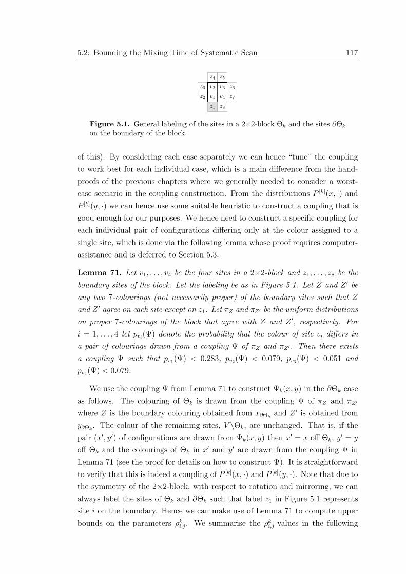
5.2: Bounding the Mixing Time of Systematic Scan 117
v1
v3
v4
v2
z2
z3
z4 z5
z6
z7
z8z1
Figure 5.1. General labeling of the sites in a 2×2-block Θk and the sites ∂Θk
on the boundary of the block.
of this). By considering each case separately we can hence “tune” the coupling
to work best for each individual case, which is a main difference from the hand-
proofs of the previous chapters where we generally needed to consider a worst-
case scenario in the coupling construction. From the distributions P [k](x, ·) and
P [k](y, ·) we can hence use some suitable heuristic to construct a coupling that is
good enough for our purposes. We hence need to construct a specific coupling for
each individual pair of configurations differing only at the colour assigned to a
single site, which is done via the following lemma whose proof requires computer-
assistance and is deferred to Section 5.3.
Lemma 71. Let v1, . . . , v4 be the four sites in a 2×2-block and z1, . . . , z8 be the
boundary sites of the block. Let the labeling be as in Figure 5.1. Let Z and Z ′ be
any two 7-colourings (not necessarily proper) of the boundary sites such that Z
and Z ′ agree on each site except on z1. Let πZ and πZ′ be the uniform distributions
on proper 7-colourings of the block that agree with Z and Z ′, respectively. For
i = 1, . . . , 4 let pvi(Ψ) denote the probability that the colour of site vi differs in
a pair of colourings drawn from a coupling Ψ of πZ and πZ′. Then there exists
a coupling Ψ such that pv1(Ψ) < 0.283, pv2(Ψ) < 0.079, pv3(Ψ) < 0.051 and
pv4(Ψ) < 0.079.
We use the coupling Ψ from Lemma 71 to construct Ψk(x, y) in the ∂Θk case
as follows. The colouring of Θk is drawn from the coupling Ψ of πZ and πZ′
where Z is the boundary colouring obtained from x∂Θkand Z ′ is obtained from
y∂Θk. The colour of the remaining sites, V \Θk, are unchanged. That is, if the
pair (x′, y′) of configurations are drawn from Ψk(x, y) then x′ = x off Θk, y′ = y
off Θk and the colourings of Θk in x′ and y′ are drawn from the coupling Ψ in
Lemma 71 (see the proof for details on how to construct Ψ). It is straightforward
to verify that this is indeed a coupling of P [k](x, ·) and P [k](y, ·). Note that due to
the symmetry of the 2×2-block, with respect to rotation and mirroring, we can
always label the sites of Θk and ∂Θk such that label z1 in Figure 5.1 represents
site i on the boundary. Hence we can make use of Lemma 71 to compute upper
bounds on the parameters ρki,j. We summarise the ρk
i,j-values in the following

118 5: Sampling 7-colourings of the Grid
(a)
j
i (b)
ji
(c)
j
i
(d)
j
i
(e)
j
i
(f)
j
i
(g)
j i
(h)
j
i
Figure 5.2. A 2×2-block Θk showing all eight positions of a site i ∈ ∂Θk onthe boundary of the block in relation to a site j ∈ Θk in the block.
Corollary of Lemma 71. Due to the symmetry of the block we can assume that
site j ∈ Θk in the corollary is located in the bottom left corner, as Figure 5.2
shows.
Corollary 72. Let Θk be any 2×2-block, let j ∈ Θk be any site in the block and
let i ∈ ∂Θk be a site on the boundary of the block. Then
ρki,j <
0.283, if i and j are positioned as in Figure 5.2(a) or (b),
0.079, if i and j are positioned as in Figure 5.2(c) or (h),
0.051, if i and j are positioned as in Figure 5.2(e) or (f),
0.079, if i and j are positioned as in Figure 5.2(d) or (g).
If i /∈ ∂Θk is not on the boundary of the block then ρki,j = 0.
Remark. Lemma 71 is stated such that, in the proof, we only need to consider
boundary colourings which is an advantage in the representation of the computer-
assisted proof. Corollary 72 provides the link between the boundary colourings
of Lemma 71 and the set of all configurations. This link is required for the proof
of Theorem 28.
Theorem 28. Let G be a finite and rectangular piece of the infinite square lattice.
Consider the systematic scan Markov chain Mgrid on Ω. The mixing time of
Mgrid is
Mix(Mgrid, ε) ≤ 63 log(nε−1)
scans of the grid. This corresponds to O(n log n) block updates since each block
is of size 4.

5.2: Bounding the Mixing Time of Systematic Scan 119
Proof. Let αk,j =∑
i ρki,j be the influence on j under Θk. We need to show
that αk,j < 1 for each block Θk and site j ∈ Θk in order to ensure that α =
maxk maxj∈Θkαk,j < 1. Fix any block Θk and any site j ∈ Θk. A site i ∈ ∂Θk on
the boundary of the block can occupy eight different positions on the boundary
in relation to j as showed in Figure 5.2(a)–(h). Thus, using the bounds from
Corollary 72 we have
αk,j =∑
i
ρki,j < 2(0.283 + 0.079 + 0.051 + 0.079) = 0.984.
Then α = maxk maxj∈Θkαk,j < maxk 0.984 = 0.984 < 1 and we obtain the stated
bound on the mixing time of Mgrid by Theorem 14.
Of course we have yet to establish a proof of Lemma 71, which is what the
subsequent section will be concerned with. Our computational proof uses some
ideas described by Goldberg et al. [33] which have been further explored by Gold-
berg, Jalsenius, Martin and Paterson [31]. In particular, we will be focusing on
minimising the probability of assigning different colours to site v1 in the couplings
constructed by our programs. We will however be required to construct a cou-
pling on the 2×2 sub-grid, rather than establishing bounds on the disagreement
probability of a site adjacent to the initial discrepancy and then extending this
to a coupling on the whole block recursively. Our approach is similar to the one
Achlioptas et al. [1] take, however we do not have the option of constructing an
“optimal” coupling using a suitable linear program (even when feasible) since our
probabilities will be maximised over all boundary colourings. The crucial differ-
ence between the approaches is that Achlioptas et al. [1] are using path coupling
as a proof technique which requires them to bound the expected Hamming dis-
tance between a pair of colourings dawn from a coupling. This in turn enables
them to specify an “optimal” coupling which minimises Hamming distance for a
given boundary colouring. We are, however, required to bound the influence of i
on j for each boundary colouring and sum over the maximum of these influences.
The reason for this is the inherit maximisation over boundary colourings in the
definition of ρki,j.
Remark. It is worth mentioning that providing bounds on the expected Ham-
ming distance is similar to showing that the influence of a site is small. Recall
that this condition is known to imply rapid mixing of a random update Markov
chain (see for example Weitz [55]). In a single-site setting the condition “the
influence of a site is small” also implies rapid mixing of systematic scan (Dyer

120 5: Sampling 7-colourings of the Grid
et al. [18]) however in a block setting it is not sufficient to give rapid mixing of
systematic scan as we discussed in Section 3.5 of Chapter 3 which is why we need
to bound the influence on a site.
5.3 Constructing the Coupling by Machine
In order to prove Lemma 71 we will construct a coupling Ψ of πZ and πZ′ for all
pairs of boundary colourings Z and Z ′ that are identical on all sites except for site
z1. Recall that πZ and πZ′ are the uniform distributions on proper 7-colourings
of the block that agree with Z and Z ′ respectively. For each coupling constructed
we verify that the probabilities pvi(Ψ), i = 1, . . . , 4, are within the bounds of the
lemma. The method is well suited to be carried out with computer-assistance
and we have implemented a C-program to do so. For details of the program see
http://www.csc.liv.ac.uk/~kasper/grid_scan/. Before stating the proof of
Lemma 71 we will discuss how a coupling can be represented by an edge-weighted
complete bipartite graph. We make use of this representation of Ψ in the proof
of the lemma.
5.3.1 Representing a Coupling as a Bipartite Graph
Let U be a set of objects and let W be a set of |U | pairs (s, ωs) such that s ∈ U
and ωs ≥ 0 is a non-negative value representing the weight of s. Each element
s ∈ U is contained exactly once in W . If the value ωs is an integer (which it is in
our case) it can be regarded as the multiplicity of s in a multiset. The set W is
referred to as a weighted set of U . Let πU,W be the distribution on U such that
the probability of s is proportional to ωs, where (s, ωs) ∈ W . More precisely, the
probability of s in πU,W is PrπU,W(s) = ωs/
∑(t,ωt)∈W ωt. For example, let W be
a weighted set of U and let U ′ ⊆ U be a subset of U . Assume the weight ωs = 0
if s ∈ U\U ′ and ωs = k if s ∈ U ′, where k > 0 is a positive constant. Then πU,W
is the uniform distribution on U ′.
The reason for introducing the notion of a weighted set is that it can be used
when specifying a coupling of two distributions. Let U be a set and let W and W ′
be two weighted sets of U such that the sum of the weights in W equals the sum
of the weights in W ′. Let ωtotal denote this sum. That is, ωtotal =∑
(s,ωs)∈W ωs =∑(s′,ω′
s′ )∈W ′ ω′s′ . The two weighted sets W and W ′ define two distributions πU,W
and πU,W ′ on U . We want to specify a coupling Ψ of πU,W and πU,W ′ . Let K|U |,|U |be an edge-weighted complete bipartite graph with vertex sets W and W ′. That

5.3: Constructing the Coupling by Machine 121
is, for each pair (s, ωs) ∈ W there is an edge to every pair (s′, ω′s′) ∈ W ′. Every
edge e of K|U |,|U | has a weight ωe ≥ 0 such that the following condition holds. Let
(s, ωs) be any pair in W ∪W ′ and let E be the set of all |U | edges incident to
(s, ωs). Then∑
e∈E ωe = ωs. It follows that the sum of the edge weights of all |U |2edges in K|U |,|U | is ωtotal. The idea is that K|U |,|U | represents a coupling Ψ of πU,W
and πU,W ′ . In order to draw a pair of elements from Ψ we randomly select an edge
e in K|U |,|U | proportional to its weight. The endpoints of e represent the elements
in U drawn from πU,W and πU,W ′ . More precisely, the probability of choosing
edge e in K|U |,|U | with weight ωe is ωe/ωtotal. If edge e = ((s, ωs), (s′, ω′s′)) is
chosen it means that we have drawn s from πU,W and s′ from πU,W ′ , the marginal
distributions of Ψ.
The bipartite graph representation of a coupling will be used when we con-
struct couplings of colourings of 2×2-blocks in the proof of Lemma 71.
5.3.2 Proof of Lemma 71
Lemma 71. Let v1, . . . , v4 be the four sites in a 2×2-block and z1, . . . , z8 be the
boundary sites of the block. Let the labeling be as in Figure 5.1. Let Z and Z ′ be
any two 7-colourings (not necessarily proper) of the boundary sites such that Z
and Z ′ agree on each site except on z1. Let πZ and πZ′ be the uniform distributions
on proper 7-colourings of the block that agree with Z and Z ′, respectively. For
i = 1, . . . , 4 let pvi(Ψ) denote the probability that the colour of site vi differs in
a pair of colourings drawn from a coupling Ψ of πZ and πZ′. Then there exists
a coupling Ψ such that pv1(Ψ) < 0.283, pv2(Ψ) < 0.079, pv3(Ψ) < 0.051 and
pv4(Ψ) < 0.079.
Proof. Fix two boundary colourings Z and Z ′ that differ on site z1. Let c be
the colour of site z1 in Z and let c′ 6= c be the colour of z1 in Z ′. Let QZ and
QZ′ be the two sets of proper 7-colourings of the block that agree with Z and
Z ′, respectively. Let Q be the set of all proper 7-colourings of the block without
taking a boundary colouring into account. Let WZ and WZ′ be two weighted sets
of Q. The weights are assigned as follows.
• For the pair (x, ωx) ∈ WZ let the weight ωx = |QZ′ | if x ∈ QZ , otherwise
let ωx = 0.
• For the pair (x, ωx) ∈ WZ′ let the weight ωx = |QZ | if x ∈ QZ′ , otherwise
let ωx = 0.

122 5: Sampling 7-colourings of the Grid
It follows from the assignment of the weights that the distribution πQ,WZis the
uniform distribution on QZ . That is, πQ,WZ= πZ . Similarly, πQ,WZ′ is the uniform
distribution πZ′ on QZ′ . Note that the sum of the weights is |QZ ||QZ′| in both WZ
and WZ′ . Then a coupling Ψ of πQ,WZand πQ,WZ′ can be specified with an edge-
weighted complete bipartite graph K = K|Q|,|Q|. For a given valid assignment to
the weights of the edges of K, making K represent a coupling Ψ, we can compute
the probability of assigning different colours to a site vi within the block in two
configurations drawn from Ψ. Let EK be the set of all edges e = ((x, ωx), (x′, ω′x′))
in K such that x and x′ differ on site vi. Then pvi(Ψ) =
∑e∈EK
ωe/|QZ ||QZ′ |.In order to obtain sufficiently small upper bounds on pvi
(Ψ) for the four sites
v1, . . . , v4 in the block we would like to assign weights to the edges of K such
that much weight is assigned to edges between colourings that agree on many
sites in the block. In general it is not clear exactly how to assign weights to the
edges. For instance, if we assign too much weight to edges between colourings
that are identical on site v2 we might not be able to assign as much weight as we
would like to on edges between colourings that are identical on site v4. Thus, the
probability of assigning different colours to site v4 would increase. Intuitively a
good strategy would be to assign as much weight as possible to edges between
colourings that are identical on the whole block. This implies that we try to
assign as much weight as possible to edges between colourings that are identical
on site v1, the site adjacent to the discrepancy site z1 on the boundary. If site v1
is assigned different colours it should be a good idea to assign as much weight as
possible to edges between colourings that are identical on the whole block apart
from site v1. This idea leads to a heuristic in which the assignment of the edge
weights is divided into three phases. The exact procedure is described as follows.
In phase one we match identical colourings. For all colourings x ∈ Q of the
block the edge e = ((x, ωx), (x, ω′x)) in K will be given weight ωe = min(ωx, ω′x).
That is, we maximise the probability of drawing the same colouring x from both
πQ,WZand πQ,WZ′ .
For the following two phases we define an ordering of the colourings in Q. We
order the colourings lexicographically with respect to the site order v3, v2, v4, v1.
That is, if the seven colours are 1, . . . , 7 the colouring of v3, v2, v4, v1 will start
with 1, 1, 1, 1, respectively. The next colouring will be 1, 1, 1, 2, and so on. This
ordering of colourings in Q carries over to an ordering of the pairs in WZ and
WZ′ . That is, we order the pairs (x, ωx) in WZ with respect to the lexicographical
ordering of x. Similarly we order the pairs in WZ′ . This ordering of the pairs will
be important in the next two phases. It provides some control of how colourings

5.4: Partial Results for 6-colourings of the Grid 123
are being paired up in terms of the assignment of the weights on edges between
pairs. Edges will be considered with respect to this ordering because choosing an
arbitrary ordering of the edges would not necessarily result in probabilities pvi(Ψ)
that would be within the bounds of the lemma.
In the second phase we ignore the colour of site v1 and match colourings that
are identical on all of the remaining three sites v2, v3 and v4. More precisely, for
each pair (x, ωx) ∈ WZ , considered in the ordering explained above, we consider
the edges e = ((x, ωx), (x′, ω′x′)) where x ∈ Q and x′ ∈ Q are identical on all
sites but v1. The edges are considered in the ordering of the second component
(x′, ω′x′) ∈ WZ′ . We assign as much weight as possible to e such that the total
weight on edges incident to (x, ωx) ∈ WZ does not exceed ωx and such that the
total weight on edges incident to (x′, ω′x′) ∈ WZ′ does not exceed ω′x′ . Note that
in the lexicographical ordering of the colourings, site v1 is the least significant site
and therefore the ordering provides some level of control of pairing up colourings
that are similar on the remaining three sites. It turns out that the resulting
coupling is sufficiently good for proving the lemma.
In the third and last phase we assign the remaining weights on the edges. As in
phase two, for each pair (x, ωx) ∈ WZ we consider the edges e = ((x, ωx), (x′, ω′x′)).
The pairs and edges are considered in accordance with the ordering explained
above. The difference between the second and third phase is that now we do not
have any restrictions on the colourings x and x′. We assign as much weight as
possible to e such that the total weight on edges incident to (x, ωx) ∈ WZ does
not exceed ωx and such that the total weight on edges incident to (x′, ω′x′) ∈ WZ′
does not exceed ω′x′ . After phase three we have assigned all weights to the edges
of K and hence K represents a coupling Ψ of πZ and πZ′ .
From K we compute the probabilities pv1(Ψ), pv2(Ψ), pv3(Ψ) and pv4(Ψ) as
described above. We have written a C-program which loops through all (non-
symmetric) colourings Z and Z ′ of the boundary of the block and constructs
the bipartite graph K as described above. For each boundary the probabilities
pv1(Ψ), pv2(Ψ), pv3(Ψ) and pv4(Ψ) are successfully verified to be within the bounds
of the lemma. For details on the C-program, see http://www.csc.liv.ac.uk/
~kasper/grid_scan/.
5.4 Partial Results for 6-colourings of the Grid
As we have seen, a systematic scan on the grid using 2×2-blocks and seven colours
mixes rapidly. An immediate question is whether we can do better and show rapid

124 5: Sampling 7-colourings of the Grid
mixing with six colours which is possible in the random update case. This matter
will be discussed in this section and we will show that, even with bigger block
sizes (up to 3×3), it is not possible to show rapid mixing using the technique of
this paper. More precisely, we will establish lower bounds on the parameter α
for 2×2-blocks, 2×3-blocks and 3×3-blocks. All three lower bounds are greater
than one and hence we cannot make use of Theorem 14 to show rapid mixing.
5.4.1 Establishing Lower Bounds for 2×2 Blocks
We start by examining the 2×2-block again but this time with six colours.
Lemma 71 provides upper bounds (under any colourings of the boundary) on
the probabilities of having discrepancies at each of the four sites of the block
when two 7-colourings are drawn from the specified coupling. For six colours we
will show lower bounds on these probabilities under any coupling and a specified
pair of boundary colourings. Once again, let v1, . . . , v4 be the four sites in a 2×2-
block and let z1, . . . , z8 be the boundary sites of the block and let the labeling
be as in Figure 5.1. Let Z and Z ′ be any two 6-colourings of the boundary sites
that assign the same colour to each site except for z1. Let πZ and πZ′ be the
uniform distributions on the sets of proper 6-colourings of the block that agree
with Z and Z ′, respectively. Let Ψminvk
(Z, Z ′) be a coupling of πZ and πZ′ that
minimises pvk(Ψ). That is, pvk
(Ψ) ≥ pvk(Ψmin
vk(Z, Z ′)) for all couplings Ψ of πZ
and πZ′ . Also let plowvk
= maxZ,Z′ pvk(Ψmin
vk(Z,Z ′)). We can hence say that there
exist two 6-colourings Z and Z ′ of the boundary of a 2×2 block, that assign the
same colour to each site except for z1, such that pvk(Ψ) ≥ plow
vifor any coupling
Ψ of πZ and πZ′ . We have the following lemma, which is proved by computation.
Lemma 73. Consider 6-colourings of the 2×2-block in Figure 5.1. Then plowv1≥
0.379, plowv2≥ 0.107, plow
v3≥ 0.050 and plow
v4≥ 0.107.
Proof. Fix one site vk in the block and fix two colourings Z and Z ′ of the boundary
of the block that differ only on the colour of site z1. Let QZ and QZ′ be the two
sets of proper 6-colourings of the block that agree with Z and Z ′, respectively.
For c = 1, . . . , 6 let nc be the number of colourings in CZ in which site vk is
assigned colour c. Similarly let n′c be the number of colourings in QZ′ in which
site vk is assigned colour c. It is clear that the probability that vk is assigned
colour c in a colouring x′ drawn from πZ is PrπZ(x′vk
= c) = nc/|QZ |. For
c = 1, . . . , 6 define mc = nc|QZ′|, m′c = n′c|QZ | and M = |QZ ||QZ′ |. It follows
that PrπZ(x′vk
= c) = mc/M and PrπZ′ (y′vk
= c) = m′c/M , where x′ and y′ are

5.4: Partial Results for 6-colourings of the Grid 125
colourings drawn from πZ and πZ′ , respectively. Observe that the quantities mc,
m′c and M can be easily computed for a given pair of boundary colourings.
Now let Ψ be any coupling of πZ and πZ′ . The probability that site vk
is coloured c in both colourings drawn from Ψ is be at most min(mc,m′c)/M .
Therefore, the probability of drawing two colourings from Ψ such that the colour
of site vk is the same in both colourings is at most∑
c=1,...,6 min(mc,m′c)/M ,
and the probability of assigning different colours to site vk is at least pvk(Ψ) ≥
1 − ∑c=1,...,6 min(mc,m
′c)/M . We have successfully verified the bounds in the
statement of the lemma by maximising the lower bound on pvk(Ψ) over all bound-
ary colourings Z and Z ′ for each site vk in the block. The computations are carried
out with the help of a computer program written in C. For details on the program,
see http://www.csc.liv.ac.uk/~kasper/grid_scan/.
For seven colours, Corollary 72 makes use of Lemma 71 to establish upper
bounds on the influence parameters ρki,j. These parameters are used in the proof
of Theorem 28 to obtain an upper bound on the parameter α. The upper bound
on α is shown to be less than one which implies rapid mixing for seven colours
when applying Theorem 14. We can use Lemma 73 to obtain lower bounds on
the influence parameters ρki,j by completing the coupling in a way analogous to
the coupling in Corollary 72. This in turn will result in a lower bound on the
parameter α that is greater than one. That is, following the proof of Theorem 28
and making use of Lemma 73, a lower bound on α will be
α ≥ 2(0.379 + 0.107 + 0.050 + 0.107) = 1.286 > 1.
Hence we fail to show rapid mixing of systematic scan with six colours using
2×2-blocks using this approach.
5.4.2 Bigger Blocks
We failed to show rapid mixing of systematic scan with six colours and 2×2-blocks
and we will now show that increasing the block size to both 2×3 and 3×3 will
not be sufficient either when using the technique from Theorem 14. Lemma 74
below considers 2×3-blocks and is analogous to Lemma 73. We make use of the
same notation as for Lemma 73, only the block is bigger and the labeling of the
sites is different (see Figure 5.3(a)). Lemma 74 is proved by computation in the
same way as Lemma 73. For details on the C-program used in the proof, see
http://www.csc.liv.ac.uk/~kasper/grid_scan/.

126 5: Sampling 7-colourings of the Grid
(a)
v1 v3v2z2
z3
z4 z5 z6
z7
z8
z1 z9z10
v4 v5 v6
(b)
j
i
i
i
i i
i
i
i
(c)
j
i
i
Figure 5.3. (a) General labeling of the sites in a 2×3-block Θk and the sites∂Θk on the boundary of the block. (b)–(c) All ten positions of a site i ∈ ∂Θk
on the boundary of the block in relation to a site j ∈ Θk in the corner of theblock.
Lemma 74. Consider 6-colourings of the 2×3-block in Figure 5.3(a). Then
plowv1≥ 0.3671, plow
v3≥ 0.0298, plow
v4≥ 0.0997 and plow
v6≥ 0.0174.
We will now use Lemma 74 to show that α > 1 for 2×3 blocks. Let Θk be any
2×3-block and let j ∈ Θk be a site in a corner of the block. A site i ∈ ∂Θk on
the boundary of the block can occupy ten different positions on the boundary in
relation to j. See Figure 5.3(b) and (c). We can again determine lower bounds
on the influences ρki,j of i on j under Θk from Lemma 74. However, Lemma 74
provides lower bounds on ρki,j only when i ∈ ∂Θk is adjacent to a corner site of the
block, as in Figure 5.3(b). If i is located as in Figure 5.3(c) we do not know more
than that ρki,j is bounded from below by zero. Nevertheless, the lower bound on
α exceeds one. Let αk,j =∑
i ρki,j be the influence on j under Θk. Following the
proof of Theorem 28 and using the lower bounds in Lemma 74 we have
αk,j =∑
i in Fig. 5.3(b)
ρki,j +
∑
i in Fig. 5.3(c)
ρki,j
≥ 2(0.3671 + 0.0298 + 0.0997 + 0.0174) = 1.028,
where we set the lower bound on the second sum to zero. Now,
α = maxk
maxj∈Θk
αk,j ≥ 1.028 > 1.
Hence we cannot use Theorem 14 to show rapid mixing of systematic scan with
six colours and 2×3-blocks. It is interesting to note that considering 2×3-blocks
was sufficient for Achlioptas et al. [1] to prove mixing of a random update Markov
chain for sampling 6-colourings of the grid.
Lastly, we increase the block size to 3×3 and show that a lower bound on
α is still greater than one. We have the following lemma which is proved by
computation in the same way as Lemmas 73 and 74.

5.4: Partial Results for 6-colourings of the Grid 127
(a)
v1 v3v2z2
z3
z4
z5 z6 z7
z8
z1
z9
z10
v4 v5 v6
z12 z11
v7 v8 v9
(b)
v1 v3v2
z2
z3
z4
z5
z6 z7 z8
z9
z10v4 v5 v6
z12
z11
v7 v8 v9
z1 (c)
j
i
i
i i
i
i
i
i
(d)
j
i
i
i
i
Figure 5.4. (a)–(b) General labeling of the sites in a 3×3-block Θk and twodifferent labellings of the sites ∂Θk on the boundary of the block. The discrep-ancy site on the boundary has label z1. (b)–(c) All twelve positions of a sitei ∈ ∂Θk on the boundary of the block in relation to a site j ∈ Θk in the cornerof the block.
Lemma 75. For 6-colourings of the 3×3-block with sites labeled as in Figure 5.4(a)
we have plowv1≥ 0.3537, plow
v3≥ 0.0245, plow
v7≥ 0.0245 and plow
v9≥ 0.0071. Further-
more, for 6-colourings of the 3×3-block in Figure 5.4(b) we have plowv1
≥ 0.0838,
plowv3≥ 0.0838, plow
v7≥ 0.0138 and plow
v9≥ 0.0138.
Note that Lemma 75 provides lower bounds on the probabilities of having a
mismatch on a corner site of the block when the discrepancy site on the boundary
(labeled z1) is adjacent to a corner site (Figure 5.4(a)) and adjacent to a middle
site (Figure 5.4(b)). Let Θk be any 3×3-block and let j ∈ Θk be a site in a corner
of the block. A site i ∈ ∂Θk on the boundary of the block can occupy twelve
different positions on the boundary in relation to j. See Figure 5.4(c) and (d).
Analogous to Corollary 72 lower bounds on the influences ρki,j of i on j under
Θk can be determined from Lemma 75. Let αk,j =∑
i ρki,j be the influence on
j under Θk. Following the proof of Theorem 28 and using the lower bounds in
Lemma 75 we have
αk,j =∑
i in Fig. 5.4(c)
ρki,j +
∑
i in Fig. 5.4(d)
ρki,j
≥ 2(0.3537 + 0.0245 + 0.0245 + 0.0071)
+(0.0838 + 0.0838 + 0.0138 + 0.0138)
= 1.0148.
Thus, α = maxk maxj∈Θkαk,j ≥ 1.0148 > 1. Hence, we cannot use Theorem 14
to show rapid mixing of systematic scan with six colours and 3×3-blocks.
A natural question is whether we can show rapid mixing using even bigger
blocks. It seems possible to do this although the computations rapidly become
intractable as the block size increases. Already with a 3×3-block the number
of boundary colourings we need to consider (after removing isomorphisms) is in

128 5: Sampling 7-colourings of the Grid
excess of 106 and for each boundary colouring there are more than 107 colourings
of the block to consider. In addition to simply generating the distributions on
colourings of the block, the time it would take to actually construct the required
couplings, as we did in the proof of Lemma 71, would also increase. Finally when
using a larger block size, different positions of site j in the block need to be
considered whereas we could make use of to the symmetry of the 2×2-block to
only consider one position of site j in the block. If different positions of j have
to be considered this has to be captured in the construction of the coupling and
would likely require more computations.
The above discussion suggests that in order to show rapid mixing for six
and fewer colours of systematic scan on the grid one may need to rely on a
different proof technique than Dobrushin uniqueness in the form of Theorem 14.
Furthermore, the fact that path coupling can be used to show rapid mixing of
a random update Markov chain for 6-colourings of the grid seems to support
this view. It is also possible that the condition in Theorem 14 is currently too
strong. Other possible conditions were discussed in Section 3.5 of Chapter 3, but
it remains on open question to see if a weaker condition would be sufficient to
establish a proof of Theorem 14.

Chapter 6
Single-site Systematic Scan for
Bipartite Graphs
In this chapter we study the mixing time of a systematic scan that makes single-
site updates. We take advantage of the fact that the underlying graph is bipartite
by fixing the scan order such that each site in the first colour class is updated
before updating the sites in the other colour class.
6.1 Preliminaries
Let G = (V, E) be any bipartite graph with maximum degree ∆. We denote the
colour classes of G by L(V ) and R(V ). Let C = 1, · · · , q be the set of colours
and Ω be the set of proper q-colourings of G. Recall from Chapter 2 that MLR
is the systematic scan Markov chain which makes the following transitions
1. for each v ∈ L(V ) make a Metropolis move on site v
2. for each v ∈ R(V ) make a Metropolis move on site v.
Recall from Example 11 that a single-site Metropolis move on site v (and given
a configuration x) is made by selecting a colour c uniformly at random from C
and recolouring site v with colour c. Let x′ be the configuration obtained from x
by recolouring site v to c. If no edge containing v is monochromatic in x′ then
the resulting configuration of the Metropolis move is x′, otherwise output of the
Metropolis move is configuration x. Finally we remind the reader that each site
in L(V ) is assigned weight ωl = q3 − 4 and each site in R(V ) is assigned weight
ωr = 2ωl − 4. We will prove Theorem 30 namely
129

130 6: Single-site Systematic Scan for Bipartite Graphs
Theorem 30. Let G be any bipartite graph with maximum vertex-degree ∆ ≥ 3.
Consider the systematic scan Markov chain MLR on the state space Ω. Let γ =
ωr
(1 + 1
q3
)− ∆ωl
q− ∆ωr
q− ∆2ωr
q2 where ωl = q3 − 4 and ωr = 2ωl − 4. If q ≥ 2∆
then γ > 0 and the mixing time of MLR is
Mix(MLR, ε) ≤ ωr log(nωrε−1)
γ
scans.
As a final piece of notation we let xj denote the configuration obtained by
one partial scan of MLR (starting from configuration x) where site j is the next
site to be updated. For a configuration xj and a colour c let (xj ↑ c) be the
configuration obtained from the following two step process. Let σ be the config-
uration obtained from xj by assigning colour c to site j. If no edge containing
site j is monochromatic in σ then (xj ↑ c) = σ, otherwise (xj ↑ c) = xj. The
reason for introducing this notation is that a Metropolis move on site j can now
be formulated as follows. Select a colour c ∈ C uniformly at random and let
xj+1 = (xj ↑ c).
Our method of proof will be path coupling using weighted Hamming distance
as the metric.
6.2 Definition of the Coupling
We begin by defining the coupling that we will use in the proof. We define the
coupling for pairs of configurations (x, y) ∈ Si which differ only on the colour
assigned to site i. We consider the update of a site j.
When it is time to update site j it is possible that more than one site is
coloured differently in xj and yj due to previous updates that have been made
in the scan. Suppose that j has k neighbour sites which are assigned different
colours in xj and yj. Let these sites be denoted by j1, . . . , jk. Note that if k = 0
then we can couple the configuration (xj ↑ c) with (yj ↑ c) for each c ∈ C which
ensures that x′j = y′j. Similarly if xjj 6= yj
j (which is only the case when i = j) we
also couple the choice (xj ↑ c) with (yj ↑ c) for each c ∈ C which may cause site
i to become a discrepancy. Otherwise xjj = yj
j and we construct the coupling as
follows. For each site jk′ where k′ ∈ 1, . . . , k make the following choices:
• If
xj
jk′ 6∈ xjj1 , . . . , x
j
jk′−1 , yjj1 , . . . , y
j
jk′−1

6.2: Definition of the Coupling 131
and
yj
jk′ 6∈ xjj1 , . . . , x
j
jk′−1 , yjj1 , . . . , y
j
jk′−1
then couple the choice of (xj ↑ xj
jk′ ) = xj with the choice (yj ↑ yj
jk′ ) = yj
in order to ensure that site j is assigned the same colour in both x′ and
y′. Also couple the choice (xj ↑ yj
jk′ ) with the choice (yj ↑ xj
jk′ ) which may
cause site j to be coloured differently in x′ and y′.
• If
xj
jk′ 6∈ xjj1 , . . . , x
j
jk′−1 , yjj1 , . . . , y
j
jk′−1
and
yj
jk′ ∈ xjj1 , . . . , x
j
jk′−1 , yjj1 , . . . , y
j
jk′−1
then couple the choice (xj ↑ xj
jk′ ) with the choice (yj ↑ xj
jk′ ). This may
cause site j to be coloured differently in x′ and y′.
• If
xj
jk′ ∈ xjj1 , . . . , x
j
jk′−1 , yjj1 , . . . , y
j
jk′−1
and
yj
jk′ 6∈ xjj1 , . . . , x
j
jk′−1 , yjj1 , . . . , y
j
jk′−1
then couple the choice (xj ↑ yj
jk′ ) with the choice (jj ↑ yj
jk′ ). This may
cause site j to be coloured differently in x′ and y′.
For any remaining colours c ∈ C \ xjj1 , . . . , x
jjk , y
jj1 , . . . , y
jjk, couple the choice
(xj ↑ c) with the choice (yj ↑ c) which ensures that the same colour is assigned
to site j in x′ and y′. This completes the coupling construction since each colour
c ∈ C has been used exactly once.
By construction of the coupling, the marginal distribution is correct since each
colour is used exactly once in both (x ↑ ·) and (y ↑ ·). We now state and prove
an upper bound on the probability of a site which is coloured the same in x and y
receiving different colours in x′ and y′ obtained from one complete scan of MLR
starting from (x, y) ∈ Si.
Lemma 76. Suppose that (x, y) ∈ Si. Obtain a pair of configurations (x′, y′) by
one complete scan of MLR starting from (x, y). Let b(j) be the number of sites
adjacent to site j that are coloured differently in xj and yj. Then for any j 6= i
Pr(x′j 6= y′j | b(j) = k) ≤ k
q.

132 6: Single-site Systematic Scan for Bipartite Graphs
Proof. In the construction of the coupling each site which is coloured differently
in xj and yj is considered exactly once and will match one of the three stated
cases. Each of these cases will produce at most one assignment of a colour to j in
each copy such that x′j 6= y′j. There are k such sites and thus at at most k such
choices will exist in the joint distribution, each being selected with probability
1/q. Hence the probability of site j being coloured differently in x′ and y′ is at
most kq.
6.3 Proof of Mixing
We first consider the case when the original discrepancy is in the left colour class
of G, and hence the site containing the original discrepancy is updated before it
can percolate to any of its neighbour sites.
Lemma 77. Suppose that (x, y) ∈ Si. Obtain a pair of configurations (x′, y′) by
one complete scan of MLR starting from (x, y). If i ∈ L(V ) then
E [Ham(x′, y′)] ≤(
1− β
ωl
)Ham(x, y)
where
β = ωl − ∆
q
(ωl +
∆ωr
q
).
In particular, when q ≥ 2∆ then β > 0.
Proof. We begin by showing that if i ∈ L(V ) then E [Ham(x′, y′)] ≤ ∆q
(ωl + ∆ωr
q
).
Since all sites in L(V ) are updated before R(V ), site i will be updated before any
of its neighbours and hence (xi, yi) ∈ Si. Since site i has at most ∆ neighbours
it will be coloured differently in x′ and y′ with probability at most ∆/q and
contribute ωl to the weighted Hamming distance.
Suppose that site i is coloured differently in each copy when the sites in R(V )
are being updated. Then each of i’s neighbour sites will be coloured differently in
x′ and y′ with probability at most 1/q by Lemma 76 and each will contribute with
weight ωr to the weighted Hamming distance. Adding it up we get the stated
bound on the expectation since site i has at most ∆ neighbours.
The statement of the lemma now follows since i ∈ L(V ) implies Ham(x, y) =
ωl and using the assumption q ≥ 2∆ gives
β ≥ ωl − ∆
2∆
(ωl +
∆ωr
2∆
)= 1 > 0

6.3: Proof of Mixing 133
by substituting the definition of ωr, which completes the proof.
We now consider the case when the initial discrepancy is in the colour class
R(V ), and hence the discrepancy can percolate to the neighbours of site i before
i is updated.
Lemma 78. Suppose that (x, y) ∈ Si and that i ∈ R(V ). Obtain a pair of
configurations (x′, y′) by one complete scan of MLR starting from (x, y). If j 6=i ∈ R(V ) and d is the number of sites in L(V ) adjacent to both i and j then
Pr(x′j 6= y′j) ≤d
q2.
Proof. Let A(j) be the random variable denoting the number of sites adjacent to
j that are coloured differently in xj and yj. Note from the statement of the lemma
that it most hold that A(j) ≤ d. From the definition of conditional probability
we have
Pr(x′j 6= y′j) =d∑
k=0
Pr (A(j) = k)Pr(x′j 6= y′j | A(j) = k).
From Lemma 76 we have Pr(x′j 6= y′j | A(j) = k) ≤ kq
so
Pr(x′j 6= y′j) ≤d∑
k=0
Pr (A(j) = k)k
q=
1
qE [A(j)] .
For each l ∈ 1, . . . , d let Il be the indicator random variable denoting the event:
xjl 6= yj
l and pl = Pr(xjl 6= yj
l ) be the probability of that event occurring. Using
linearity of expectation
Pr(x′j 6= y′j) ≤1
qE
[d∑
l=1
Il
]=
1
q
d∑
l=1
E [Il] =1
q
d∑
l=1
pl.
From Lemma 76 we obtain pl ≤ 1q
for l ∈ 1, . . . , d since site i is the only site
adjacent to l that is coloured differently in xl and yl. Thus,
Pr(x′j 6= y′j) ≤1
q
d∑
l=1
1
q=
d
q2
which completes the proof.

134 6: Single-site Systematic Scan for Bipartite Graphs
Lemma 79. Suppose that (x, y) ∈ Si. Obtain a pair of configurations (x′, y′) by
one complete scan of MLR starting from (x, y). If i ∈ R(V ) then
E [Ham(x′, y′)]− ωrPr(x′i 6= y′i) ≤∆ωl
q+
∆(∆− 1)ωr
q2.
Proof. From Lemma 76 we know that the expected number of additional discrep-
ancies in L(V ) is at most ∆/q since site i has at most ∆ neighbour sites, each
of which will be coloured differently in each copy with probability at most 1/q.
Each of those sites has weight ωl.
To upper bound the expected number of additional discrepancies in R(V ) we
need to upper bound the number of sites in L(V ) adjacent to both i and some
j 6= i ∈ R(V ). We let d(v, u) denote the minimum distance (number of edges)
between site u and v in G, and u v the existence of an edge between u and v.
The sum over all j 6= i ∈ R(V ) of the number of sites adjacent to both i and j is
thus
∑j∈V
d(i,j)=2
∑
k∈Vkjki
1 =∑
k∈Vki
∑j∈Vj 6=ijk
1
≤∑
k∈Vki
(∆− 1)
≤ ∆(∆− 1).
Combining this bound with Lemma 78 we have, by linearity of expectation, that
the expected number of additional disagreements in R(V ) is at most (∆−1)∆q2 each
of which has weight ωr.
We now need to upper bound the probability of site i being coloured differently
in x′ and y′. To that end we introduce the following terminology.
Definition 80 (Colour compatibility). Let N(v) be the set of sites adjacent to a
site v, and let
C(v) = C \⋃
v′∈N(v)
xv′ , yv′
be the set of colours not adjacent to v. Two distinct sites k and l are said to be
‘colour compatible’ if C(k) ∩ C(l) 6= ∅.

6.3: Proof of Mixing 135
Lemma 81. Suppose (x, y) ∈ Si for some i ∈ R(V ). Let N(v) be the set of sites
adjacent to a site v. If deg i = ∆ and q ≥ ∆ + 3 then there are two distinct sites
vk ∈ N(i) and vl ∈ N(i) which are colour compatible.
Proof. For ease of reference, let N(i) = v1, . . . , v∆ and also let c(v) be the size
of the set C(v). Each site v ∈ N(i) has at most ∆ neighbours. Since site i is the
only site that contributes two colours to C \ C(v) it holds that
c(v) ≥ q − (∆− 1)− 2 = q −∆− 1 (6.1)
for every v ∈ N(i). We need to show the existence of two distinct sites vk and vl
that are colour compatible. We will do this by contradiction. Suppose that no
two sites in N(i) are colour compatible. Then
C(vk) ⊆ C \⋃
vl∈N(i)l<k
C(vl) (6.2)
for all k ∈ 1, . . . , ∆ since otherwise some site vl ∈ v1, . . . , vk−1 would be
colour compatible with site vk. By (6.2), C(vk) cannot contain any of the colours
in ⋃
vl∈N(i)l<k
C(vl).
Also, it cannot contain xi or yi so
c(vk) = q −∑
0<l<k
c(vl)− 2 ≤ q − (k − 1)(q −∆− 1)− 2
by (6.1). Hence
q −∆− 1 ≤ c(v∆) ≤ q − (∆− 1)(q −∆− 1)− 2
where the lower bound is from (6.1).
When ∆ ≥ 3 it follows that q ≤ ∆+2 which contradicts our assumption that
q ≥ ∆ + 3. Hence there must be a pair of colour compatible sites in N(i).
Lemma 82. Suppose (x, y) ∈ Si for some i ∈ R(V ). Let N(i) be the set of sites
adjacent to site i. If deg i = ∆ and q ≥ ∆ + 3 then there are two sites k ∈ N(i)
and l ∈ N(i) such that
Pr (xik = xi
l = yik = yi
l) ≥1
q2.

136 6: Single-site Systematic Scan for Bipartite Graphs
Proof. By Lemma 81 there exist two distinct sites k and l in N(i) that are colour
compatible. Since k and l are colour compatible there is at least one colour c
that will be accepted when updating both sites k and l. With probability at
least 1/q, colour c will be selected and accepted in the recolouring of site k and
independently with probability at least 1/q in the recolouring of site l.
Lemma 83. Suppose that (x, y) ∈ Si. Obtain a pair of configurations (x′, y′) by
one complete scan of MLR starting from (x, y). If i ∈ R(V ) then
Pr(x′i 6= y′i) ≤∆(q + 1)
q2− 1
q3.
Proof. Let A(i) be the random variable denoting the number of sites in N(i) that
are assigned different colours in configuration xi and yi. Note from the statement
of the lemma that it most hold that A(i) ≤ ∆. From the definition of conditional
probability we have
Pr(x′i 6= y′i) =∆∑
k=0
Pr(A(i) = k)Pr(x′i 6= y′i | A(i) = k).
We consider the two cases deg i = ∆ and deg i ≤ ∆ − 1 separately. First
suppose deg i ≤ ∆ − 1. If there are k sites adjacent to i that are assigned
different colours xi and yi then there can be at most ∆− 1 + k different colours
adjacent to site i. Hence Pr(x′i 6= y′i | A(i) = k) ≤ ∆−1+kq
which gives
Pr(x′i 6= y′i) ≤∆−1∑
k=0
Pr(A(i) = k)∆− 1 + k
q
=∆− 1
q
∆−1∑
k=0
Pr(A(i) = k) +1
qE [A(i)]
=∆− 1
q+
1
qE [A(i)]
by definition of probability spaces.
Now for each l ∈ 1, . . . , deg i let Il be the indicator random variable denoting
the event: xil 6= yi
l . Also let pl = Pr(xil 6= yi
l) be the probability that the event

6.3: Proof of Mixing 137
occurs. Using linearity of expectation we have
Pr(x′i 6= y′i) ≤∆− 1
q+
1
qE
[deg i∑
l=1
Il
]
=∆− 1
q+
1
q
deg i∑
l=1
E [Il]
=∆− 1
q+
1
q
deg i∑
l=1
pl.
From Lemma 76 we have pl ≤ 1/q for l ∈ 1, . . . , deg i since site i is the only
site adjacent to l in that can be coloured differently in xl and yl. Thus,
Pr(x′i 6= y′i) ≤∆− 1
q+
1
q
deg i∑
l=1
1
q
=∆− 1
q+
deg i
q2
≤ (∆− 1)(q + 1)
q2.
Now consider the case when deg i = ∆. As before, define N(i) as the set of
sites adjacent to i. Let Ei be shorthand for the following event: There exists two
distinct sites a ∈ N(i) and b ∈ N(i) such that xia = xi
b = yia = yi
b. If there are k
sites adjacent to i that are assigned different colours in xi and yi then there can
be at most ∆ + k different colours adjacent to site i. However, if Ei holds there
can be at most ∆+ k− 1 different colours adjacent to i since two sites are known
to have the same colour. Hence
Pr(x′i 6= y′i | A(i) = k) ≤ Pr (Ei | A(i) = k)∆ + k − 1
q
+ (1− Pr (Ei | A(i) = k))∆ + k
q
=∆ + k
q− Pr (Ei | A(i) = k)
1
q.

138 6: Single-site Systematic Scan for Bipartite Graphs
Proceeding as in the previous case
Pr(x′i 6= y′i) ≤∆∑
k=0
Pr(A(i) = k)
(∆ + k
q− Pr(Ei | A(i) = k)
1
q
)
=∆∑
k=0
Pr(A(i) = k)∆ + k
q−
∆∑
k=0
Pr(A(i) = k)Pr(Ei | A(i) = k)1
q
=∆
q
∆∑
k=0
Pr(A(i) = k) +1
qE [A(i)]
− 1
q
∆∑
k=0
Pr(A(i) = k)Pr(Ei | A(i) = k)
=∆
q+
1
qE [A(i)]− 1
qPr(Ei)
by definition of probability spaces and observing that 0 ≤ A(i) ≤ ∆.
Again let Il be the indicator random variable denoting the event: xil 6= yi
l
defined for each l ∈ 1, . . . , ∆. Also let pl = Pr(xil 6= yi
l) be the probability that
the event occurs. Using linearity of expectation
Pr(x′i 6= y′i) ≤∆
q+
1
qE
[∆∑
l=1
Il
]− 1
qPr(Ei)
=∆
q+
1
q
∆∑
l=1
E [Il]− 1
qPr(Ei)
=∆
q+
1
q
∆∑
l=1
pl − 1
qPr(Ei).
From Lemma 76 we have pl ≤ 1/q for l ∈ 1, . . . , ∆ since site i is the only site
adjacent to l in that can be coloured differently in xl and yl. Thus,
Pr(x′i 6= y′i) ≤∆
q+
1
q
∆∑
l=1
1
q− 1
qPr(Ei)
=∆
q+
∆
q2− 1
qPr(Ei)
=∆(q + 1)
q2− 1
qPr(Ei)

6.3: Proof of Mixing 139
and so
Pr(x′i 6= y′i) ≤ max
((∆− 1)(q + 1)
q2,∆(q + 1)
q2− 1
qPr(Ei)
)
=∆(q + 1)
q2− 1
qPr(Ei)
which can be verified by letting Pr(Ei) ≤ 1. Finally we have Pr(Ei) ≥ 1/q2 from
Lemma 82 which completes the proof.
Lemma 84. Suppose that (x, y) ∈ Si and ∆ ≥ 3. Obtain a pair of configurations
(x′, y′) by one complete scan of MLR starting from (x, y). If i ∈ R(V ) then
E [Ham(x′, y′)] ≤(
1− γ
ωr
)Ham(x, y)
where
γ = ωr
(1 +
1
q3
)− ∆ωl
q− ∆ωr
q− ∆2ωr
q2.
In particular, when q ≥ 2∆ then γ ≥ 1− 12q3 > 0.
Proof. From Lemmas 79 and 83 we have
E [Ham(x′, y′)] ≤ ∆ωl
q+
ωr(∆− 1)∆
q2+ ωr
(∆(q + 1)
q2− 1
q3
)
=∆ωl
q+
∆ωr
q+
∆2ωr
q2− ωr
q3
by expanding and simplifying.
Given that i ∈ R(V ) we have Ham(x, y) = ωr which implies the definition of
γ in the statement of the lemma. Finally use the assumption q ≥ 2∆ to verify
γ ≥ ωr
(1 +
1
q3
)− ωl
2− ωr
2− ωr
4
=2ωl − q3 − 4
q3
= 1− 12
q3> 0
using ωr = 2ωl − 4 and ωl = q3 − 4 and the fact that q ≥ 6.
This enables us to prove Theorem 30.
Proof of Theorem 30. Suppose that (x, y) ∈ Si and obtain a pair of configurations
(x′, y′) by one complete scan ofMLR starting from (x, y). From Lemmas 77 and 84

140 6: Single-site Systematic Scan for Bipartite Graphs
we have
E [Ham(x′, y′)] ≤ max
(Ham(x, y)
(1− γ
ωr
), Ham(x, y)
(1− β
ωl
))
= Ham(x, y)
(1−min
(γ
ωr
,β
ωl
))
= Ham(x, y)
(1− γ
ωr
)< Ham(x, y)
since γ > 0 from Lemma 84. The claim that min(
γωr
, βωl
)= γ
ωrcan be verified
since 3 ≤ ∆ ≤ q2. This bound on the expected value of Ham(x′, y′) implies
Theorem 30 by Corollary 9 (path coupling).

Chapter 7
Conclusion
This thesis has been concerned with analysing the mixing time of systematic scan
Markov chains. We conclude by summarising the contributions this thesis has
made to the field of computer science as well as highlighting some open problems
it poses.
Summary of Contributions
The main contribution of this thesis has been the introduction of a new technique
for bounding the mixing time of systematic scan Markov chains using block dy-
namics. This technique involves providing sufficiently good upper bounds on an
influence parameter which represents the maximum influence on a site of the un-
derlying graph. These bounds are derived through the construction of a coupling
for the update of each block starting from two configurations that are identical
except for on the spin assigned to a single site. This influence parameter is often
simple to compute for a given coupling. If the maximum influence on a site is
sufficiently small then the systematic scan Markov chain mixes in O(log n) scans.
This new technique has the immediate advantage that one is not required to keep
track of intermediate states of the chain during the analysis. A further advantage
that this proof technique has is that it implies rapid mixing of systematic scan for
any order of the given set of blocks whereas path coupling is specific to the stated
order. The new proof technique is based on a known technique called Dobrushin
uniqueness and the main result (Theorem 14) was proved in Chapter 3. The
condition on the influence parameter that needs to be satisfied when applying
this technique is a generalisation of a similar condition that applies to single-site
dynamics as we discussed in Section 3.5 of Chapter 3.
We have presented several applications of this technique in this thesis and
141

142 7: Conclusion
they all reduce the gap between the parameters that imply mixing for random
update and systematic scan. In summary these applications were
• systematic scan for sampling from the uniform distribution on proper q-
colourings of general graphs with maximum vertex-degree ∆ mixes in O(log n)
scans whenever q ≥ 2∆ (Theorem 16 which was proved in Chapter 3),
• systematic scan for sampling from the uniform distribution on proper q-
colourings of a height-H tree mixes in O(H) scans whenever q > ∆ +
2√
∆− 1 in the single-site case and in fewer colours using some suitable
block dynamics (Theorems 18 and 20 which were proved in Chapter 3),
• systematic scan for sampling from the uniform distribution on proper 7-
colourings the grid mixes in O(log n) scans (Theorem 28 which was proved
in Chapter 5), and
• systematic scan for sampling from the uniform distribution on H-colourings
of the n-vertex path mixes in O(log n) scans whenever H has a 2-edge path
between all vertices (Theorem 22 which was proved in Chapter 4).
We have also used path coupling in some cases when the underlying graph of the
spin system could help to facilitate an analysis. In summary these results were
• a systematic scan Markov chain for sampling for the uniform distribution
of H-colourings of the n-vertex path mixes in O(log n) scans for any fixed
H (Theorem 24 proved in Chapter 4), and
• a single-site systematic scan Markov chain for sampling from the uniform
distribution of proper q-colourings of a general bipartite graphs with max-
imum vertex-degree ∆ mixes in O(log n) scans whenever q ≥ 2∆ (Theo-
rem 30 proved in Chapter 6).
A determining factor that helped significantly to facilitate the coupling analysis of
the two systematic scan Markov chains mentioned above was the structure of the
underlying graph. In the case of the systematic scan for sampling H-colourings
of the path, the fact that the underlying graph is a path clearly makes it more
feasible to keep track of any discrepancies that percolate during each individual
scan. In the case of proper q-colourings of bipartite graphs we were able to scan
each colour class of the underlying graph separately which significantly limited
the set of sites that could potentially have become discrepancies during one scan.

Open Problems 143
Finally the results for sampling H-colourings of the path using systematic
scan created a temporary gap between the parameters required for mixing of
systematic scan and random update. This gap was closed by the following result
about a random update Markov chain which was included for completeness
• a random update Markov chain for sampling for the uniform distribution
of H-colourings of the n-vertex path mixes in O(n log n) block updates for
any fixed H (Theorem 26 proved in Chapter 4).
Open Problems
Despite the improvements in the parameters that imply mixing of systematic scan
for various spin systems presented in this thesis, the gap between the parameters
sufficient for mixing of systematic scan and random update still persists (although
in many cases the gap is now somewhat reduced). For example, in the case
when the spin system correspond to proper q-colourings of a general graph with
maximum vertex-degree ∆ then the condition q ≥ (11/6)∆ is sufficient for rapid
mixing of a random update Markov chain (Vigoda [53]) whereas the corresponding
condition required for rapid mixing of systematic scan is q ≥ 2∆ (Theorem 16).
Similar gaps also exist for special graphs such as trees or the grid and it is of
general interest to either close those gaps or to show that systematic scan does
not mix under the same conditions as random update. The possibility of the
latter, namely that systematic scan does not mix under the same conditions as
random update, is however unlikely. Currently the only types of examples where
there is a genuine difference between the mixing properties of systematic scan
and random update is the relatively uninteresting case when the spin system
corresponds to proper colourings of a graph with no edges (where random update
requires Ω(n log n) updates but systematic scan mixes in one scan) or contrived
examples such as the spin system in Observation 53 (where random update mixes
rapidly but systematic scan does not mix at all).
Another open problem that arises from the work presented in this thesis is
whether the condition required for mixing in Theorem 14 is too strong. The
possibility of using other conditions was explored to some depth in Section 3.5 of
Chapter 3, however it remains possible that a weaker condition on the influence
on a site could be sufficient to prove rapid mixing of systematic scan. Note
that it may be possible to develop conditions that hold for certain spin systems
such as proper q-colourings but not for general spin systems, and such conditions

144 7: Conclusion
would also be of interest. A final open problem related to Theorem 16, which
was also raised in Chapter 3, is whether it is possible to find a general method
for obtaining a set of weights that would make the influence on a site sufficiently
small provided that the influence of a site is small. This would be a generalisation
of the matrix balancing in the single-site case as we have previously discussed.
Note that we do rule out the possibility of finding such a set of weights when
using a natural definition of “the influence of a site” that is similar to the path
coupling condition. None the less, it remains possible that a stronger definition
of “the influence of a site” would make it possible to find such a set of weights
(see Observation 54 and the remark following it).

Bibliography
[1] Dimitris Achlioptas, Mike Molloy, Cristopher Moore, and Frank van Bussel.Sampling grid colourings with fewer colours. In LATIN, pages 80–89, 2004.
[2] David Aldous. Random walks on finite groups and rapidly mixing Markovchains. In Seminaire de probabilites XVII, pages 243–297. Springer-Verlag,1983.
[3] David Aldous and James Fill. Reversible Markov chains and random walkson graphs. http://www.stat.berkeley.edu/users/aldous/RWG/book.html.
[4] Magnus Bordewich, Martin Dyer, and Marek Karpinski. Stopping times,metrics and approximate counting. In Michele Bugliesi, Bart Preneel,Vladimiro Sassone, and Ingo Wegener, editors, ICALP, volume 4051 of Lec-ture Notes in Computer Science, pages 108–119. Springer, 2006.
[5] Russ Bubley and Martin Dyer. Path coupling: a technique for proving rapidmixing in Markov chains. In FOCS, pages 223–231. IEEE Computer Society,1997.
[6] Russ Bubley, Martin Dyer, and Catherine S. Greenhill. Beating the 2∆bound for approximately counting colourings: A computer-assisted proof ofrapid mixing. In SODA, pages 355–363. ACM/SIAM, 1998.
[7] Robert Burton and Jeffrey Steif. Nonuniqueness of measures of maximalentropy for subshifts of finite type. Ergodic Theory and Dynamical Systems,14(2):213–236, 1994.
[8] Colin Cooper, Martin Dyer, and Alan Frieze. On Markov chains for randomlyH-colouring a graph. Journal of Algorithms, 39(1):117–134, 2001.
[9] Mary Kathryn Cowles and Bradley P. Carlin. Markov chain Monte Carloconvergence diagnostics: A comparative review. Journal of The AmericanStatistical Association, 91(434):883–904, 1996.
[10] Mary Kathryn Cowles, Gareth O. Roberts, and Jeffrey S. Rosenthal. Possiblebiases induced by MCMC convergence diagnostics. Journal of StatisticalComputation and Simulation, 64:87–104, 1999.
[11] Persi Diaconis and Arun Ram. Analysis of systematic scan Metropolis al-gorithms using Iwahoti-Hecke algebra techniques. Michigan MathematicalJournal, 48:157–190, 2000.
145

146 Bibliography
[12] Roland Lvovich Dobrushin. Prescribing a system of random variables byconditional distributions. Theory of Probability and Its Applications, 15:458–486, 1970.
[13] Roland Lvovich Dobrushin and Senya B. Shlosman. Constructive criterionfor the uniqueness of Gibbs field. In Jozsef Fritz, Arthur Jaffe, and DomokosSzasz, editors, Statistical mechanics and dynamical systems, volume 10 ofProgress in Physics, pages 371–403. Birkhauser, Boston, 1985.
[14] Martin Dyer, Alan Frieze, and Mark Jerrum. On counting independent setsin sparse graphs. SIAM Journal on Computing, 31(5):1527–1541, 2002.
[15] Martin Dyer, Leslie Ann Goldberg, Catherine Greenhill, and Mark Jerrum.On the relative complexity of approximate counting problems. Algorithmica,38(3):471–500, 2003.
[16] Martin Dyer, Leslie Ann Goldberg, Catherine S. Greenhill, Mark Jerrum,and Michael Mitzenmacher. An extension of path coupling and its appli-cation to the glauber dynamics for graph colourings. SIAM Journal onComputing, 30(6):1962–1975, 2001.
[17] Martin Dyer, Leslie Ann Goldberg, and Mark Jerrum. Counting and sam-pling H-colourings. Information and Computation, 189:1–16, 2004.
[18] Martin Dyer, Leslie Ann Goldberg, and Mark Jerrum. Dobrushin conditionsand systematic scan. In Josep Dıaz, Klaus Jansen, Jose D. P. Rolim, andUri Zwick, editors, APPROX-RANDOM, volume 4110 of Lecture Notes inComputer Science, pages 327–338. Springer, 2006.
[19] Martin Dyer, Leslie Ann Goldberg, and Mark Jerrum. Matrix norms andrapid mixing for spin systems. arXiv:math.PR/0702744 (submitted), 2006.
[20] Martin Dyer, Leslie Ann Goldberg, and Mark Jerrum. Systematic scan andsampling colourings. Annals of Applied Probability, 16(1):185–230, 2006.
[21] Martin Dyer, Leslie Ann Goldberg, Mark Jerrum, and Russell Martin.Markov chain comparison. Probability Surveys, 3:89–111, 2006.
[22] Martin Dyer and Catherine Greenhill. A more rapidly mixing Markov chainfor graph colourings. Random Structures and Algorithms, 13:285–317, 1998.
[23] Martin Dyer and Catherine S. Greenhill. Random walks on combinatorialobjects. In J. D. Lamb and D. A. Preece, editors, Surveys in Combinatorics,volume 267 of London Mathematical Society Lecture Notes Series, pages 101–136. Cambridge University Press, 1999.
[24] Martin Dyer and Catherine S. Greenhill. The complexity of counting graphhomomorphisms. Random Structures and Algorithms, 17:260–289, 2000.
[25] Martin Dyer and Catherine S. Greenhill. On Markov chains for independentsets. Journal of Algorithms, 35(1):17–49, 2000.

Bibliography 147
[26] Martin Dyer, Alistair Sinclair, Eric Vigoda, and Dror Weitz. Mixing in timeand space for lattice spin systems: A combinatorial view. Random Structuresand Algorithms, 24(4):461–479, 2004.
[27] George S. Fishman. Coordinate selection rules for gibbs sampling. TheAnnals of Applied Probability, 6(2):444–465, 1996.
[28] Hans Follmer. A covariance estimate for Gibbs measures. Journal of Func-tional Analysis, 46(3):387–395, 1982.
[29] Anna Galluccio, Pavol Hell, and Jaroslav Nesetril. The complexity of H-colouring of bounded degree graphs. Discrete Mathematics, 222:101–109,2000.
[30] Hans-Otto Georgii. Gibbs Measures And Phase Transitions. de GruyterStudies in Mathematics 9. Walter de Gruyter & Co, 1998.
[31] Leslie Ann Goldberg, Markus Jalsenius, Russell Martin, and Mike Paterson.Improved mixing bounds for the anti-ferromagnetic potts model on Z2. LMSJournal of Computation and Mathematics, 9:1–20, 2006.
[32] Leslie Ann Goldberg, Steven Kelk, and Mike Paterson. The complexity ofchoosing an H-colouring (nearly) uniformly at random. SIAM Journal onComputing, 33(2):416–432, 2004.
[33] Leslie Ann Goldberg, Russell Martin, and Mike Paterson. Strong spatialmixing for lattice graphs with fewer colours. SIAM Journal on Computing,35(2):486–517, 2005.
[34] Leslie Ann Goldberg, Russell Martin, and Mike Paterson. Random samplingof 3-colourings in Z2. Random Structures and Algorithms, 24(3):279–302,2004.
[35] Geoffrey Grimmett and David Stirzaker. Probability and Random Processes.Oxford University Press, 3rd edition, 2001.
[36] Thomas P. Hayes. A simple condition implying rapid mixing of single-sitedynamics on spin systems. In FOCS, pages 39–46. IEEE Computer Society,2006.
[37] Pavol Hell and Jaroslav Nesetril. On the complexity of H-colouring. Journalof Combinatorial Theory, Series B, 48:92–110, 1990.
[38] Markus Jalsenius and Kasper Pedersen. A systematic scan for 7-colouringsof the grid. arXiv:0704.1625 (submitted), 2007.
[39] Mark Jerrum. A very simple algorithm for estimating the number of k-colourings of a low-degree graph. Random Structures and Algorithms, 7:157–165, 1995.

148 Bibliography
[40] Mark Jerrum. Counting, sampling and integrating: algorithms and complex-ity. Birkhauser, 2003.
[41] Mark Jerrum, Leslie G. Valiant, and Vijay V. Vazirani. Random genera-tion of combinatorial structures from a uniform distribution. TheoreticalComputer Science, 43:169–188, 1986.
[42] Frank P. Kelly. Stochastic models of computer communication systems.Journal of the Royal Statistical Society: Series B (Statistical Methodology),47:370–395, 1985.
[43] Claire Kenyon, Elchanan Mossel, and Yuval Peres. Glauber dynamics ontrees and hyperbolic graphs. In FOCS, pages 568–578. IEEE ComputerSociety, 2001.
[44] Michael Luby, Dana Randall, and Alistair Sinclair. Markov chain algorithmsfor planar lattice structures. SIAM Journal on Computing, 31:167–192, 2001.
[45] Michael Luby and Eric Vigoda. Fast convergence of the Glauber dynamicsfor sampling independent sets: Part I. Random Structures and Algorithms,15(3–4):229–241, 1999.
[46] Fabio Martinelli, Alistair Sinclair, and Dror Weitz. Glauber dynamics ontrees: Boundary conditions and mixing time. Communications in Mathe-matical Physics, 250(2):301–334, 2004.
[47] Kasper Pedersen. Dobrushin conditions for systematic scan with block dy-namics. In Ludek Kucera and Antonın Kucera, editors, MFCS, volume 4708of Lecture Notes in Computer Science, pages 264–275. Springer, Berlin, 2007.
[48] Kasper Pedersen. On systematic scan for sampling H-colourings of the path.arXiv:0706.3794 (submitted), 2007.
[49] Gareth O. Roberts and Sujit K. Sahu. Updating schemes, correlation struc-ture, blocking and parameterization for the Gibbs sampler. Journal of theRoyal Statistical Society: Series B (Statistical Methodology), 59(2):291–317,1997.
[50] Jesus Salas and Alan D. Sokal. Absence of phase transition for antiferro-magnetic Potts models via the Dobrushin uniqueness theorem. Journal ofStatistical Physics, 86:551–579, 1997.
[51] Barry Simon. The Statistical Mechanics of Lattice Gases, volume I. PrincetonUniversity Press, 1993.
[52] Leslie G. Valiant. The complexity of computing the permanent. TheoreticalComputer Science, 8:189–201, 1979.
[53] Eric Vigoda. Improved bounds for sampling colourings. Journal of Mathe-matical Physics, 41(3):1555–1569, 2000.

Bibliography 149
[54] Dror Weitz. Mixing in Time and Space for Discrete Spin Systems. PhDthesis, University of California, Berkley, 2004.
[55] Dror Weitz. Combinatorial criteria for uniqueness of Gibbs measures. Ran-dom Structures and Algorithms, 27(4):445–475, 2005.
[56] Dror Weitz. Counting independent sets up to the tree threshold. In STOC,pages 140–149. IEEE Computer Society, 2006.
[57] Benjamin Widom and John S. Rowlinson. New model for the study of liquid-vapour phase transition. The Journal of Chemical Physics, 52(4):1670–1684,1970.
Related Documents