On Space-Time Capacity Limits in Mobile and Delay Tolerant Networks

arX

iv:0

912.

3441

v1 [

cs.N

I] 1

7 D

ec 2

009

1

On Space-Time Capacity Limits in Mobile andDelay Tolerant Networks

Philippe Jacquet, Bernard Mans and Georgios Rodolakis

Abstract

We investigate the fundamental capacity limits of space-time journeys of information in mobile and DelayTolerant Networks (DTNs), where information is either transmitted or carried by mobile nodes, using store-carry-forward routing. We define the capacity of a journey (i.e., a path in space and time, from a source to a destination)as the maximum amount of data that can be transferred from thesource to the destination in the given journey.Combining a stochastic model (conveying all possible journeys) and an analysis of the durations of the nodes’encounters, we study the properties of journeys that maximize the space-time information propagation capacity,in bit-meters per second. More specifically, we provide theoretical lower and upper bounds on the informationpropagation speed, as a function of the journey capacity. Inthe particular case of random way-point-like models(i.e., when nodes move for a distance of the order of the network domain size before changing direction), we showthat, for relatively large journey capacities, the information propagation speed is of the same order as the mobilenode speed. This implies that, surprisingly, in sparse but large-scale mobile DTNs, the space-time informationpropagation capacity in bit-meters per second remains proportional to the mobile node speed and to the size of thetransported data bundles, when the bundles are relatively large. We also verify that all our analytical bounds areaccurate in several simulation scenarios.

I. INTRODUCTION

The problem of determining fundamental limits on the performance of mobile and ad hoc networks

continues to attract the interest of researchers. Several important results have been achieved with the

seminal papers by Gupta and Kumar [7] (which provided the first capacity bounds in static wireless

networks) and by Grossglauser and Tse [6] (which showed thatthe mobility can increase the capacity of

an ad hoc network). Various mobility models have been studied in the literature, and the delay-capacity

relationships under those models have been characterized (e.g., [4], [13], [15]). However, the nature of

these trade-offs is strongly influenced by the choice of the mobility model [14].

Moreover, there has been an increased interest in mobile ad hoc networks where end-to-end multi-hop

paths may not exist and communication routes may only be available through time and mobility; depending

on the context, these networks are now commonly referred as Intermittently Connected Networks (ICNs)

or Delay Tolerant Networks (DTNs). Although limited, the understanding of the fundamental properties

of such networks is steadily increasing. There is a significant number of results focusing on characterizing

the packet propagation delay [3], [5], [17], assuming that packet transmissions are instantaneous, and more

recently, the information propagation speed [8], [10], [11]. The authors of [3] took a graph-theoretical

approach in order to upper bound the time it takes for disconnected mobile networks to become connected

Part of this work will be presented in “On Space-Time Capacity Limits in Mobile and Delay Tolerant Networks”, P. Jacquet,B. Mansand G. Rodolakis, IEEE Infocom, 2010.

P. Jacquet is with INRIA, 78153 Le Chesnay, France. E-mail: [email protected]. Mans and G. Rodolakis are with Macquarie University, 2109NSW, Australia. E-mails: [email protected],

[email protected]

2

through the mobility of the nodes. The papers [5], [17] analyze the delay of common routing schemes,

such as epidemic routing, under the assumption that the inter-meeting time between pairs of nodes

follows an exponential distribution. However, this assumption is not generally verified, depending on the

relationship between the size of the network domain and the relevant time-scale of the network scenario

under consideration [1], and this can result in either an over-estimation or an under-estimation of the

actual system performance [2]. Departing from the exponential inter-meeting time hypothesis, in [10],

[11], Kong and Yeh studied the information dissemination latency in large wireless and mobile networks,

in constrained i.i.d. mobility and Brownian motion models.They showed that, when the network is not

percolated, the latency scales linearly with the Euclideandistance between the sender and the receiver. The

first analytical estimates of the constant upper bounds on the speed at which information can propagate

in DTNs, again without considering the quantity of information that can be transmitted, were obtained

in [8].

In contrast, in this paper, we investigate the space-time capacity of such networks,i.e., the maximum

amount of information that can be transferred from a source to a destination over time. As the network is

almost surely disconnected, we refer to journeys rather than paths, where a journey is an alternation of data

transmissions and carriages using store-carry-forward routing. Informally, our objective is to determine

how fast a given amount of datay can reach its destination. Formally, we use a probabilisticmodel of

space-time journeys of packets of information in DTNs (in Section II), and define the journey capacity as

well as the information propagation speed (in Section III),to provide the following main contributions:

• we characterize the duration of node meetings, by bounding the probability function of the durations

of the nodes’ encounters, in Section IV;

• we prove the first non trivial lower bounds on the informationpropagation speed (Theorem 1), for a

bounded journey capacity, in random waypoint-like mobility, in Section V;

• we prove general upper bounds on the information propagation speed (Theorem 2 and Corollaries 1

and 2), as a function of the journey capacity, and we investigate the properties of journeys that

maximize the space-time network capacity in bit-meters persecond, in Section VI;

• we compare and verify the analytical bounds with simulationmeasurements in Section VII.

We provide concluding remarks in Section VIII.

II. NETWORK AND MOBILITY MODEL

We consider a network ofn nodes in a square area of sizeA = L×L and radio rangeR. As we want

to focus on DTNs that are almost surely disconnected, we willanalyze the case whereR is fixed, while

n,A → ∞, such that the node densityν = nA is bounded by some constant.

Formally, we adopt the random geometric graph model [16]: two nodes at distance smaller than a

maximum radio rangeR can exchange information. Moreover, we consider that the rate at which nodes

can transmit data when they are within range is fixed, and equals G units of data per second.

3

Initially, the nodes are distributed uniformly at random. Every node follows an i.i.d. random trajectory,

reflected on the borders of the square (like billiard balls).The nodes change direction at Poisson rateτ and

keep a constant speedv between direction changes. The motion direction angles areuniformly distributed

in [0, 2π) and are mutually independent among all nodes. Whenτ = 0, we have apure billiard model

(nodes only change direction at the border). Whenτ > 0, we have arandom walk model; when τ → ∞we are on the Brownian limit. Whenτ = O( 1

L) → 0 we are on arandom way-point-like model, since

nodes travel a distance of orderL before changing direction or hitting the border.

III. SPACE-TIME JOURNEY ANALYSIS

We studyjourneys with a given capacity, i.e., journeys that guarantee that at least an amount of data can

be transferred to the destination. Our aim is to find the shortest journey (in time) with journey capacity at

leasty, that connects any source to any destination in the network domain, in order to derive the overall

information propagation speed.

We base our analysis on a probabilistic model of journeys of packets of information that encapsulates

all possible shortest journeys originating at the source, as used in [8]. LetC be a simple journey (i.e., a

journey not returning to the same node twice). LetZ(C) be the terminal point. LetT (C) be the time at

which the journey terminates. Letp(C) be the probability of the journeyC.

Let ζ be an inverse space vector,i.e., with components expressed in inverse distance units. Letθ be a

scalar in inverse time units. We denote byw(ζ, θ) the journey Laplace transform, defined for a domain

definition for (ζ, θ):w(ζ, θ) = E(exp(−ζ · Z(C) − θT (C)))

=∑

C p(C) exp(−ζ · Z(C) − θT (C)).

We call p(z0, z1, t) the normalized density of journeys starting fromz0 at time 0, and arriving atz1

before timet:p(z0, z1, t) =

1

R2

∑

‖z1−Z(C)‖<R,T (C)<t

p(C) .

Let us consider that a bundle of information ofy bits is generated att = 0 on a node at coordinatez0 =

(x0, y0). Let us initially consider a destination node which stays motionless at coordinatez1 = (x1, y1);

in this case,p(z0, z1, t) denotes the probability that the destination receives one bit of information before

time t. Now, let us consider a moving destination node, that is located at coordinatez1 = (x1, y1), at time

t. We denotez = z1 − z0. Let q(z, t, y) denote the probability that there exists a journey of capacity at

leasty reaching the destination before timet.

The information propagation speeds(y), considering a journey capacityy, is defined as the minimum

ratio of distance over time above which the journey probability tends to0, i.e.,

• if ||z||t> s(y), then lim||z||,t→∞ q(z, t, y) = 0;

• if ||z||t< s(y), then lim||z||,t→∞ q(z, t, y) > 0.

We also define thespace-time information propagation capacityc(y) (from now on simply referred

to as thespace-time capacity), as the maximal transport capacity in bit-meters per second, that can be

4

achieved by any journey of capacityy. Thus, in this model, the space-time capacity corresponds to the

productc(y) = s(y)y.

Therefore, in order to determine the space-time capacity limits of mobile and delay tolerant networks,

we will analyze the information propagation speed, as a function of the journey capacity; in the following

sections, we will compute lower and upper bounds. In order toderive the bounds, we first study the

characteristics of node meetings.

IV. NODE MEETINGS

A meeting (or encounter) between two nodes occurs when theirdistance becomes smaller than or equal

to R, i.e., when the nodes come into communication range.

Lemma 1:A nodeA, moving in directionψ0, meets new nodes moving in direction betweenψ1 and

ψ1 + dψ at rate:fψ1 | ψ0 = 2vνRπ

sin(ψ1−ψ0

2)dψ, for ψ0, ψ1 ∈ (−π, π], whereR is the radio range.

Proof: See appendix.

We denote the meeting duration by the random variableT .

Lemma 2:The probabilityP (T > t) that a meeting has duration at leastt satisfies:

P (T > t) ≤ min(1,π2R

8vt).

Proof: The average number of neighbors of any node isπνR2. From Lemma 1, the rate at which a

node meets new neighbors isf = 8vνRπ

. Therefore, from the Little formula, the average meeting time (i.e.,

the time that a node remains a neighbor) equalsπνR2

f= π2R

8v. The proof follows by applying Markov’s

inequality.

In the pure billiard model (i.e., when τ = 0), we can give the exact formulas on the meeting time

distribution. We note that our model where nodes bounce on the borders like billiard balls is equivalent

to considering an infinite area made of mirror images of the original network domain square: a mobile

node moves in the original square while its mirror images move in the mirror squares [8].

Lemma 3:We denote the meeting duration by the random variableT . The probability density function

pT (t) of T is:

pT (t) =1

4log

∣

∣

∣

∣

vRt+ 1

vRt− 1

∣

∣

∣

∣

(

1 +R2

(vt)2

)

− R

2vt, (1)

for t ≥ 0, wherev is the node speed,R is the radio range.

When t→ ∞, the cumulative probabilityP (T > t) is:

P (T > t) =R2

3(vt)2+O

(

R4

(vt)4

)

.

Proof: See appendix.

5

V. LOWER BOUND

We prove a lower boundsL(y) on the information propagation speed, for journey capacityy, in the

random way-point-like mobility model,i.e., when nodes travel a distance of the order of the network

domain length before changing direction. Initially, we focus on the pure billiard mobility model,i.e., we

assume that nodes do not change direction unless they hit theborder. Finally, we remark that the result

can be generalized to node mobility with a small change of direction rate.

We will show that, for all destination nodes which, at timet, are at distancer ∼ sL(y)t of the initial

source location, there is a journey of durationt and of capacityy from the source to the destination,

with probability strictly larger than0. We consider large distancesr = Θ(√n), wheren is the number

of nodes in the network; in this case, the square network domain has a side lengthr = Θ(√n), as we

are interested in the case where the node density is constant(but strictly larger than 0), as discussed in

Section II. We show that, when the journey capacity isy ≤ Kv

, for a constantK, the lower bound is

sL(y) = v, wherev is the mobile node speed.

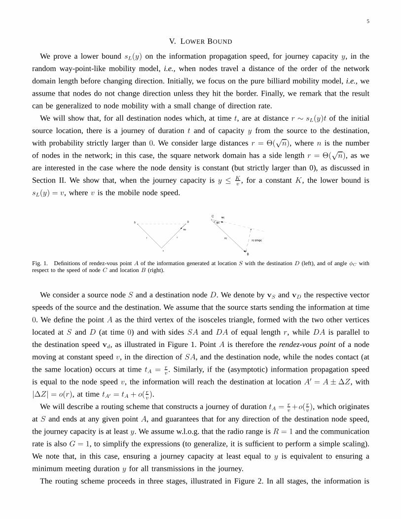
Fig. 1. Definitions of rendez-vous pointA of the information generated at locationS with the destinationD (left), and of angleφC withrespect to the speed of nodeC and locationB (right).

We consider a source nodeS and a destination nodeD. We denote byvS andvD the respective vector

speeds of the source and the destination. We assume that the source starts sending the information at time

0. We define the pointA as the third vertex of the isosceles triangle, formed with the two other vertices

located atS andD (at time 0) and with sidesSA andDA of equal lengthr, while DA is parallel to

the destination speedvd, as illustrated in Figure 1. PointA is therefore therendez-vous pointof a node

moving at constant speedv, in the direction ofSA, and the destination node, while the nodes contact (at

the same location) occurs at timetA = rv. Similarly, if the (asymptotic) information propagation speed

is equal to the node speedv, the information will reach the destination at locationA′ = A ± ∆Z, with

|∆Z| = o(r), at timetA′ = tA + o( rv).

We will describe a routing scheme that constructs a journey of durationtA = rv+o( r

v), which originates

at S and ends at any given pointA, and guarantees that for any direction of the destination node speed,

the journey capacity is at leasty. We assume w.l.o.g. that the radio range isR = 1 and the communication

rate is alsoG = 1, to simplify the expressions (to generalize, it is sufficient to perform a simple scaling).

We note that, in this case, ensuring a journey capacity at least equal toy is equivalent to ensuring a

minimum meeting durationy for all transmissions in the journey.

The routing scheme proceeds in three stages, illustrated inFigure 2. In all stages, the information is

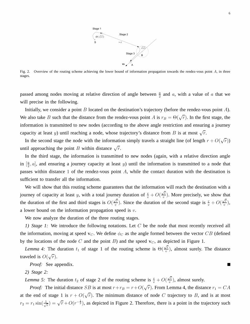
6

Fig. 2. Overview of the routing scheme achieving the lower bound of information propagation towards the rendez-vous point A, in threestages.

passed among nodes moving at relative direction of angle between a2

and a, with a value ofa that we

will precise in the following.

Initially, we consider a pointB located on the destination’s trajectory (before the rendez-vous pointA).

We also takeB such that the distance from the rendez-vous pointA is rB = Θ(√r). In the first stage, the

information is transmitted to new nodes (according to the above angle restriction and ensuring a journey

capacity at leasty) until reaching a node, whose trajectory’s distance fromB is at most√r.

In the second stage the node with the information simply travels a straight line (of lengthr +O(√r))

until approaching the pointB within distance√r.

In the third stage, the information is transmitted to new nodes (again, with a relative direction angle

in [a2, a], and ensuring a journey capacity at leasty) until the information is transmitted to a node that

passes within distance1 of the rendez-vous pointA, while the contact duration with the destination is

sufficient to transfer all the information.

We will show that this routing scheme guarantees that the information will reach the destination with a

journey of capacity at leasty, with a total journey duration ofrv

+O(√r

v). More precisely, we show that

the duration of the first and third stages isO(√r

v). Since the duration of the second stage isr

v+O(

√r

v),

a lower bound on the information propagation speed isv.

We now analyze the duration of the three routing stages.

1) Stage 1:We introduce the following notations. LetC be the node that most recently received all

the information, moving at speedvC . We defineφC as the angle formed between the vectorCB (defined

by the locations of the nodeC and the pointB) and the speedvC , as depicted in Figure 1.

Lemma 4:The durationt1 of stage 1 of the routing scheme isΘ(√r

v), almost surely. The distance

traveled isO(√r).

Proof: See appendix.

2) Stage 2:

Lemma 5:The durationt2 of stage 2 of the routing scheme isrv

+O(√r

v), almost surely.

Proof: The initial distanceSB is at mostr+rB = r+O(√r). From Lemma 4, the distancer1 = CA

at the end of stage 1 isr + O(√r). The minimum distance of nodeC trajectory toB, and is at most

r2 = r1 sin( 1√r) =

√r+O(r−

12 ), as depicted in Figure 2. Therefore, there is a point in the trajectory such

7

that the final distance of nodeC from the pointB is exactly√r. Therefore, the total distance traveled in

stage 2 is at mostr1(1 + ( 1√r)) = r +O(

√r).

3) Stage 3:At the beginning of stage 3, there is a node carrying the information, located within distance

rB +√r from the rendez-vous point, and within distance

√r from the destination’s trajectory. In this

stage, the information is transmitted to new nodes (again, according to the above angle restriction and

ensuring a capacity at leasty) until reaching a node that passes within distance1 of the rendez-vous point

A, while the contact duration with the destination is at leasty.

Equivalently to stage 1, letC be the node that most recently received all the information,moving at

speedvC . We introduce again the angleφC , this time defined with respect to the rendez-vous pointA;

namely,φC is the angle formed between the vectorCA (defined by the locations of the nodeC and the

rendez-vous pointA) and the speedvC .

Lemma 6:We consider a nodeC, at distancerC from the rendez-vous point, moving with speedvC

at a direction such that the relative angle with the destination’s direction is at mosta = 12uy

. If the angle

φC is at most 12rC

, then the trajectory ofC passes within range of the destination and guarantees that the

meeting duration with a destination located atA, moving at constant speed, will be at least equal toy.

Proof: The relative speed of the nodeC, with respect to the destination’s speed, is at most2v sin(a2) ≤

va. If the nodeC passes within distancem from the rendez-vous point, the meeting duration is at least1−mva

(since the distance traveled within range, in the frame of reference of the destination, is at least

1 − m). Therefore, in order for the meeting durationT to be at least equal toy, it is sufficient that:

m ≤ 1− yva = 12. In this case, we guarantee a meeting duration at least equalto y. Moreover, if we have

φC ≤ 12rC

, the node will pass within distance12

from the rendez-vous point.

Lemma 7:The durationt3 of stage 3 isO(√r

v), almost surely. At the end of stage 3, the destination is

reached at the rendez-vous point with probability strictlylarger than0.

Proof: See appendix.

Theorem 1:Consider a network with constant node densityν, radio rangeR and communication rate

G, where nodes move at speedv > 0 and change direction at rateτ = 0. When the journey capacity is at

mosty = Kv

, whereK is a constant, a lower bound on the information propagation speed issL(y) = v.

Proof: Considering the final position of any destination, we can define a rendez-vous pointA. If

the distance of the rendez-vous point from the source location at time0 is r → ∞, based on the previous

lemmas, there exists with strictly positive probability a journey of capacity at leasty that reaches any

rendez-vous pointA within time ∼ rv. Therefore, the asymptotic information speed is at leastv.

We note that, in case the network domainA = L × L is sufficiently large, for all destination nodes

which, at timet = Θ(L), are at distancer = o(vt) of the initial source location, there is almost surely a

journey of durationt and of capacityy from the source to the destination.

Remark 1:Although, we derived the lower bound in a pure billiard mobility model, the proof can be

easily generalized to a random walk model, where the change of direction rate isO(1r), by restarting from

the first stage at any change of direction (an event which occurs a finite number of times).

8

VI. UPPERBOUND AND SPACE-TIME CAPACITY

In this section, our aim is to find the shortest journey of capacity at leasty that connects any source to

any destination in the network domain. We prove an upper bound sU(y) on the information propagation

speed, for journeys of capacityy.Theorem 2:Consider a network withn mobile nodes with radio rangeR, communication rateG, in

a square area of sizeA = L × L, where nodes move at speedv, and change direction at rateτ . Whenn → ∞, such that the node density becomesν = n

L2 , an upper bound on the information propagationspeed, for journeys of capacityy, is the smallest ratio ofθ

ρwith:

minρ,θ>0

θ

ρwith θ =

√

√

√

√ρ2v2 +

(

τ +γ(y)4πvνRI0(ρR)

1 − γ(y)πνR2ρ

I1(ρR)

)2

− τ

,

whereI0() andI1() aremodified Bessel functions, and,

• γ(y) = min(π2RG8vy

, 1), if τ > 0;

• γ(y) = min( (RG)2

3(vy)2, 1), if τ = 0.

Remark 2:The expression ofθ has meaning whenπνR2γ(y) < 1. Above this threshold, the upper

bound for the information propagation speed is infinite. Such a behavior is expected, since there exists

a critical node density above which the graph is fully connected or at least percolates [12]. In addition,

according to Theorem 2, in percolated networks, there is a critical journey capacityyc, such that, when

y > yc, the propagation speed is bounded by a constant.

Proof: We assume that a source starts emitting information at position z = 0 and timet = 0. We

consider the probabilistic space-time journey model presented in Section III, which includes all shortest

journeys originating at the source. Equivalently, we modeljourneys of very small beacons of information,

such that beacon transmissions are instantaneous.

We initially consider an infinite network with a Poisson density of nodesλ. We will upper bound

the probability density of journeys in the infinite network model. However, by applying an analytical

depoissonization technique [9], we obtain an equivalent asymptotic estimate of the journey density when

the number of nodesn is large but not random.

We decompose the journeys into two types of segments, modeling node movements and beacon trans-

missions:

• emission segmentsSe(u,v): the node transmits immediately after receiving the beacon; v is the speed

of the node that just received the beacon, andu is the emission space vector and is such that|u| ≤ R;

• move-and-emit segmentsSm(u,v,w) = M(v,w)+u: M(v,w) is the space-time vector correspond-

ing to the motion of the node carrying the beacon, wherev is the initial vector speed of the node

when it receives the beacon andw is the final speed of the node just before transmitting the beacon;

the vectoru is the emission space vector which ends the segment.

Considering any sequence of segments, we can always upper bound the segment probabilities (see [8],

Section III-B). In fact, the conditional probabilities, given the node direction and speed, are upper bounded

by unconditional probabilities:

9

• P̃ (Se(u)) = P (u)λ, whereP (u) is the probability density ofu inside the disk of radiusR, andλ

is the node density (to make the emission possible);

• P̃ (Sm(u,v,w)) = P (u)P (M(v,w))2vλ, whereP (u) is the probability density ofu on the circle

of radiusR (we only need to consider the earliest transmissions, whichoccur at the maximum radio

range),P (M(v,w)) is the probability that the node movement equals the space vector M(v,w),

andv is the node speed.

This upper bound journey model results in a higher density ofjourneys than in the actual network. But,

in this model, any journey can be decomposed into a sequence of independent segments. Consequently,

we can express a journeyC as an arbitrary sequence of emissionor move-and-emit segments,i.e., using

regular expression notation,C = (Se + Sm)∗. Moreover, we can calculate the Laplace transform of the

journey probability density, based on the Laplace transforms of the segments. We denote the segment

Laplace transforms byle(ζ, θ) = E(e−(ζ,θ)·Se) and lm(ζ, θ) = E(e−(ζ,θ)·Sm), for emission and move-and-

emit segments, respectively. Equivalently to the formal identity 11−x = 1+x+x2+x3+..., which represents

the Laplace transform of an arbitrary sequence of random variables with Laplace transformx, the journey

Laplace transform has a denominatork(ζ, θ), equal to:

k(ζ, θ) = 1 − (le(ζ, θ) + lm(ζ, θ)) . (2)

We have the following Laplace transform expressions:

• le(ζ, θ) = E(e−ζ·u), whereu is uniform in the disk of radiusR, with densityλ, i.e., le(ζ, θ) =

λπ 2R|ζ| I1(|ζ |R).

• le(ζ, θ) = E(e−ζ·u)E(e−(ζ,θ)·M(v,w)), whereu is uniform on the circle of radiusR, with densityλ,

i.e.,E(e−ζ·u) = 2πλRI0(|ζ |R), andE(e−σ·M(v,w)) = 1√(θ+τ)2−|ζ|2v2−τ

(see [8]).

We derive an upper bound on the information propagation speed, in the special case where the journey

capacity isy = 0, from the analysis of the singularities of the journey Laplace transform, forλ equal to

the node density in the network (cf. Theorem 1 in [8]). The upper bound is the smallest ratioθρ

of the

non-negative pair(ρ, θ) which is a root of the denominatork(ρ, θ) (with ρ = |ζ |), obtained by substituting

the segment Laplace transforms expressions in (2).

In order to generalize to journeys of a given capacityy > 0, we will restrict the set of possible

journeys, to those satisfying the desired capacity constraint, and calculate the Laplace transform of the

journey density in this restricted set.

First, we remark that, a journey has a capacity at leasty, if and only if the journeythickness(i.e., the

minimum duration of all data transmissions in the journey) is at least equal toyG

, withG the communication

rate. Therefore, when considering journeys of a given capacity, we can equivalently focus on the possible

journeys with minimum node meeting durationyG

.

Therefore, in the upper-bound journey model, we can substitute the probability of any emission segment

with the probability of the same emission segment, while additionally ensuring that the emission duration

is at least yG

. Thus, for the singularity analysis, we substitute in (2) the Poisson densityλ with a node

10

densityνγ(y), whereγ(y) is an upper bound on the probability that the meeting duration is at leastyG

.

This direct substitution is feasible because we work with the upper bound journey model, where successive

segments (including all transmissions) are independent ofthe previous network state. Again, this results in

considering a higher density of journeys than in the actual network (including some transmissions which

are not actually possible, due to the node directions); however, there is no impact on the validity of our

analysis, since we are interested in upper bounds.

To conclude the proof, it suffices to substitute quantityγ(y) using Lemma 3 whenτ = 0, and Lemma 2

when τ > 0.

We derive the following corollaries expressing the behavior of the upper bound when the journey

capacity is large, in random waypoint-like (τ → 0) and random walk/Brownian motion mobility (τ > 0),

respectively.

Corollary 1: When nodes move at speedv > 0, and νy→ 0 (i.e., the journey capacityy is large) with

τ > 0, the propagation speed upper bound isO(√

νGyτRv).

Proof: See appendix.

Corollary 2: When the node speed isv > 0, and νy→ 0 (i.e., the journey capacityy is large) with

τ = O( 1L) → 0, the propagation speed upper bound isv +O(τ + νGR2

y).

Proof: See appendix.

We observe that, for large journey capacitiesy, the upper bound on the information propagation speed

sU(y) tends to the actual mobile node speedv in random way-point-like mobility, while it decreases with

the inverse square root of the journey capacityy in random walk or Brownian motion mobility. In both

cases, the resulting upper bound on the space-time capacityc(y) = sU(y)y is a function which increases

with y.

Remark 3:When nodes move at speedv > 0 in random way-point-like mobility:

• from Theorem 1, a lower bound on the propagation speed isv, for any boundedy, and when the

node density isν = Θ(1);

• from Corollary 2, an upper bound on the propagation speed isv, for journey capacitiesy such that

ν = o(y).

Therefore, we notice that there is a range of values ofy, for which our bounds are almost tight. More

generally, we deduce that the information propagation speed in random way-point-like mobility models

is of the same order as the mobile node speed, for (bounded) journey capacities that are relatively large

with respect to the node density.

This implies that, in sparse but large-scale mobile DTNs, the space-time information propagation

capacity in bit-meters per second remains proportional to the mobile node speed and to the size of the

transported data bundles, when the bundles are relatively large. It is rather surprising that the propagation

speed does not tend to0 when the size of the bundles increases, which would result ina sub-linear

increase of the space-time capacity.

11

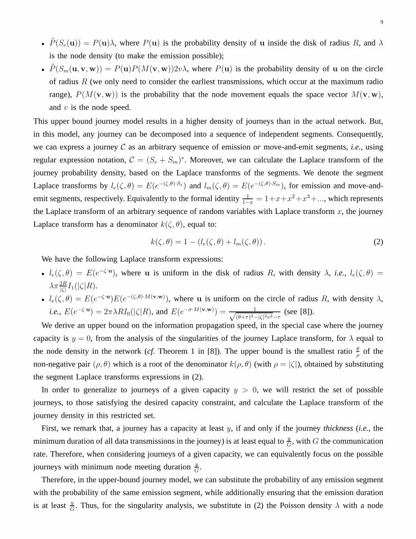
Fig. 3. Snapshots of simulated information propagation at three different times (t = 100, 170, 240), for a small journey capacityy = 0.5(top) and a larger journey capacityy = 2.5 (bottom). Larger black squares represent nodes that have received all the information at the timeof the snapshot.

VII. N UMERICAL RESULTS

In this section, we perform simulation measurements to compare to the analytical bounds on the

information propagation, derived in the previous sections. We developed a simulator that follows the

network and mobility model described in Section II. We simulate the epidemic broadcast of information,

and we consider journeys with a given lower bound on the capacity y, as described in Section III. We note

that the simulation is more general than the simple broadcast of a packet of sizey, since the information

can also be transferred on a given journey using smaller packets. In fact, we precisely ensure that the

journeys of the simulated broadcast have a capacity at leasty, without imposing further restrictions. For

all the following simulations, we consider a communicationrateG = 1 units of data per second (e.g.,

if one unit of data corresponds tox Mbits, the journey capacity in the following examples should be

multiplied by x Mbits).

We first show how information propagates in a full epidemic broadcast, by illustrating two typical

and distinct situations, depending on the journey capacityy. In the simulated scenario, a source starts

broadcasting information at timet = 50, in a network of5000 nodes, in a2000m× 2000m square, with

radio rangeR = 10m, and mobile node speedv = 5m/s, with pure billiard mobility (τ = 0). In Figure 3,

we consider two cases: a smaller journey capacityy = 0.5 (top) and a larger journey capacityy = 2.5

12

(bottom). For each case, we depict three snapshots of the simulated information propagation at three

different times,t = 100, 170, 240, from left to right. The small black dots represent the mobile nodes;

when two dots are in contact, the corresponding nodes are within communication range. The larger black

squares represent nodes that have received all the information at the time of the snapshot,i.e., those that

can be reached by a journey of capacityy. The simulation scenario is exactly the same in both the top

and bottom figures, with the only change concerning the journey capacities. In both cases, the location

of the source is approximately located at the center of the disk containing the black squares, at the top

left figure. We observe that, at the top row of Figure 3 corresponding to a small journey capacity, the

information propagates as a full disk that grows at a constant rate, which coincides with the information

propagation speed; all nodes inside the disk can be reached by a journey of capacityy, almost surely.

Equivalently, this means that the average information propagation delay scales linearly with the distance

from the source, and the ratio of the propagation delay over the distance is equal to the inverse of the

information propagation speed. On the other hand, at the bottom row, corresponding to a larger journey

capacity, only some of the nodes inside the disk have been reached by a journey of capacityy. In this

case, the average information propagation delay does not necessarily scale linearly with the distance from

the source. However, the information still propagates at a (smaller than before) maximum speed, equal to

the rate at which the disk radius grows.

Next, we simulate a network of500 nodes, moving in an area600m×600m, with a radio range of10m,

a mobile node speed of5m/s and a communication rateG = 1 units of data per second. We simulate

two different mobility parameters (rates of direction change): τ = 0 for the pure billiard mobility model,

where nodes change direction only when they bounce on the border, andτ = 0.05 for a random walk

model.

In Figure 4 we plot the ratio of the propagation delay over thedistance from the source, versus the

distance, for journey capacitiesy = {1; 2; 3}. Each sample point in the plots corresponds to a simulation

measurement. The distance is measured from the location of the source when the information was emitted

to the location of the destination when the information was received. We notice that, for all journey

capacities, the ratio of the propagation delay over the distance is larger than a non-zero constant. The

constant lower bound on the ratio, in this simulation scenario, is close to the inverse of the mobile

node speed (which is plotted in the figures as a straight line,for comparison). Furthermore, this constant

corresponds to the upper bound on the information propagation speed, which was calculated in Theorem 2.

In fact, for small journey capacities (e.g.,y = 0.5), we notice that the upper bound on the information

propagation speed is larger than (but close to) the mobile node speed. For larger journey capacities and

τ = 0, the upper bound can be obtained from Corollary 2, and indeedcorresponds to the mobile node

speed. We also notice that, forτ = 0.05, the average distance that each node travels before changing

direction is100m, which is of the order of the square network domain length. Therefore, in this case,

the upper bound on the propagation speed also remains close to the estimate for random waypoint-like

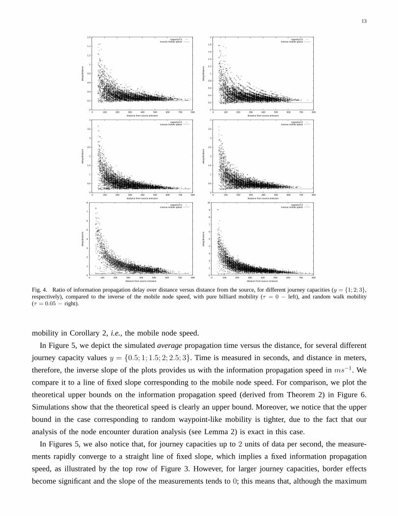
13

0

0.2

0.4

0.6

0.8

1

1.2

1.4

1.6

0 100 200 300 400 500 600 700 800

dela

y/di

stan

ce

distance from source emission

capacity1.0inverse mobile speed

0

0.2

0.4

0.6

0.8

1

1.2

1.4

1.6

1.8

2

0 100 200 300 400 500 600 700 800

dela

y/di

stan

ce

distance from source emission

capacity1.0inverse mobile speed

0

0.5

1

1.5

2

2.5

3

3.5

4

0 100 200 300 400 500 600 700 800

dela

y/di

stan

ce

distance from source emission

capacity2.0inverse mobile speed

0

0.5

1

1.5

2

2.5

3

3.5

4

0 100 200 300 400 500 600 700 800

dela

y/di

stan

ce

distance from source emission

capacity2.0inverse mobile speed

0

1

2

3

4

5

6

7

8

0 100 200 300 400 500 600 700 800

dela

y/di

stan

ce

distance from source emission

capacity3.0inverse mobile speed

0

1

2

3

4

5

6

7

8

9

10

0 100 200 300 400 500 600 700 800

dela

y/di

stan

ce

distance from source emission

capacity3.0inverse mobile speed

Fig. 4. Ratio of information propagation delay over distance versus distance from the source, for different journey capacities (y = {1; 2; 3},respectively), compared to the inverse of the mobile node speed, with pure billiard mobility (τ = 0 − left), and random walk mobility(τ = 0.05 − right).

mobility in Corollary 2, i.e., the mobile node speed.

In Figure 5, we depict the simulatedaveragepropagation time versus the distance, for several different

journey capacity valuesy = {0.5; 1; 1.5; 2; 2.5; 3}. Time is measured in seconds, and distance in meters,

therefore, the inverse slope of the plots provides us with the information propagation speed inms−1. We

compare it to a line of fixed slope corresponding to the mobilenode speed. For comparison, we plot the

theoretical upper bounds on the information propagation speed (derived from Theorem 2) in Figure 6.

Simulations show that the theoretical speed is clearly an upper bound. Moreover, we notice that the upper

bound in the case corresponding to random waypoint-like mobility is tighter, due to the fact that our

analysis of the node encounter duration analysis (see Lemma2) is exact in this case.

In Figures 5, we also notice that, for journey capacities up to 2 units of data per second, the measure-

ments rapidly converge to a straight line of fixed slope, which implies a fixed information propagation

speed, as illustrated by the top row of Figure 3. However, forlarger journey capacities, border effects

become significant and the slope of the measurements tends to0; this means that, although the maximum

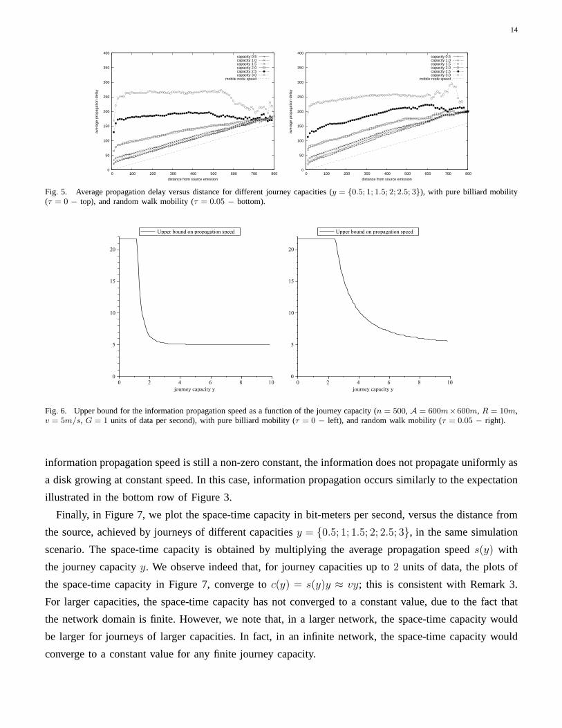
14

0

50

100

150

200

250

300

350

400

0 100 200 300 400 500 600 700 800

aver

age

prop

agat

ion

dela

y

distance from source emission

capacity 0.5capacity 1.0capacity 1.5capacity 2.0capacity 2.5capacity 3.0

mobile node speed

0

50

100

150

200

250

300

350

400

0 100 200 300 400 500 600 700 800

aver

age

prop

agat

ion

dela

y

distance from source emission

capacity 0.5capacity 1.0capacity 1.5capacity 2.0capacity 2.5capacity 3.0

mobile node speed

Fig. 5. Average propagation delay versus distance for different journey capacities (y = {0.5; 1; 1.5; 2; 2.5; 3}), with pure billiard mobility(τ = 0 − top), and random walk mobility (τ = 0.05 − bottom).

Upper bound on propagation speed

journey capacity y0 2 4 6 8 10

0

5

10

15

20

Upper bound on propagation speed

journey capacity y0 2 4 6 8 10

0

5

10

15

20

Fig. 6. Upper bound for the information propagation speed asa function of the journey capacity (n = 500, A = 600m×600m, R = 10m,v = 5m/s, G = 1 units of data per second), with pure billiard mobility (τ = 0 − left), and random walk mobility (τ = 0.05 − right).

information propagation speed is still a non-zero constant, the information does not propagate uniformly as

a disk growing at constant speed. In this case, information propagation occurs similarly to the expectation

illustrated in the bottom row of Figure 3.

Finally, in Figure 7, we plot the space-time capacity in bit-meters per second, versus the distance from

the source, achieved by journeys of different capacitiesy = {0.5; 1; 1.5; 2; 2.5; 3}, in the same simulation

scenario. The space-time capacity is obtained by multiplying the average propagation speeds(y) with

the journey capacityy. We observe indeed that, for journey capacities up to2 units of data, the plots of

the space-time capacity in Figure 7, converge toc(y) = s(y)y ≈ vy; this is consistent with Remark 3.

For larger capacities, the space-time capacity has not converged to a constant value, due to the fact that

the network domain is finite. However, we note that, in a larger network, the space-time capacity would

be larger for journeys of larger capacities. In fact, in an infinite network, the space-time capacity would

converge to a constant value for any finite journey capacity.

15

0

2

4

6

8

10

12

14

0 100 200 300 400 500 600

spac

e-tim

e ca

paci

ty (

bit.m

/s)

distance from source

journey capacity 0.5journey capacity 1.0journey capacity 1.5journey capacity 2.0journey capacity 2.5journey capacity 3.0

0

2

4

6

8

10

12

14

0 100 200 300 400 500 600

spac

e-tim

e ca

paci

ty (

bit.m

/s)

distance from source

journey capacity 0.5journey capacity 1.0journey capacity 1.5journey capacity 2.0journey capacity 2.5journey capacity 3.0

Fig. 7. Space-time capacity in bit-meters per second, versus distance from the source, for journey capacitiesy = {0.5; 1; 1.5; 2; 2.5; 3},with pure billiard mobility (τ = 0 − top), and random walk mobility (τ = 0.05 − bottom).

VIII. C ONCLUDING REMARKS

We characterized the space-time capacity limits of mobile DTNs, by providing lower (Theorem 1) and

upper bounds (Theorem 2) on the information propagation speed, with a given journey capacity. Moreover,

we verified the accuracy of our bounds with extensive simulations in several scenarios.

Such theoretical bounds are paramount in order to increase our understanding of the fundamental

properties and performance limits of DTNs, as well as to design or optimize the performance of specific

routing protocols. In fact, our results provide lower and upper bounds on the best achievable propagation

delay of bundles of data, over large distances.

It is also worth noting that our analysis provides the first known lower bounds on the information

propagation speed in mobile DTNs (for random waypoint-likemobility models), and generalize previously

known upper bounds.

More specifically, in the case of random waypoint-like mobility models, we showed that for relatively

large journey capacities, the information propagation speed is of the same order as the mobile node speed.

This implies that, in sparse but large-scale mobile DTNs, the space-time information propagation capacity

in bit-meters per second remains proportional to the mobilenode speed and to the size of the transported

data bundles, when the bundles are relatively large.

ACKNOWLEDGMENT

The authors would like to thank Matthieu Mangion for useful discussions that led to the proof of

Lemma 3.

REFERENCES

[1] H. Cai and D. Y. Eun, “Crossing over the bounded domain: from exponential to power-law inter-meeting time in Manet”, Mobicom,2007.

[2] H. Cai and D. Y. Eun, “Aging rules: what does the past tell about the future in mobile ad-hoc networks?”, MobiHoc, 2009.[3] F. De Pellegrini, D. Miorandi, I. Carreras and I. Chlamtac, “A Graph-based model for disconnected ad hoc networks”, Infocom,

2007.[4] A. El Gamal, J. Mammen, B. Prabhakar, and D. Shah, “Throughput delay trade-off in wireless networks”, Infocom, 2004.[5] R. Groenevelt, P. Nain and G. Koole, “The message delay inmobile ad hoc networks”,Performance Evaluation, Vol. 62, 2005.[6] M. Grossglauser and D. Tse, “Mobility increases the capacity of ad hoc wireless netorks”, Infocom, 2001.

16

[7] P. Gupta and P. R. Kumar, “The capacity of wireless networks”, IEEE Trans. on Info. Theory, vol. IT-46(2), pp. 388-404, 2000.[8] P. Jacquet, B. Mans and G. Rodolakis, “Information propagation speed in mobile and delay tolerant networks”, Infocom, 2009.[9] P. Jacquet and W. Szpankowski, “Analytical depoissonization and its applications”,Theoretical Computer Science, Volume 201, 1998.

[10] Z. Kong and E. Yeh, “On the latency for information dissemination in Mobile Wireless Networks”, MobiHoc, 2008.[11] Z. Kong and E. Yeh, “Connectivity and Latency in Large Scale Wireless Networks with Unreliable Links”, Infocom, 2008.[12] R. Meester and R. Roy,Continuum Percolation, Cambridge University Press, Cambridge, 1996.[13] M. J. Neely and E. Modiano, “Capacity and delay tradeoffs for ad-hoc mobile networks”, inIEEE Trans. on Information Theory,

2005.[14] G. Sharma, R. Mazumdar and N. Shroff, “Delay and capacity trade-offs in mobile ad hoc networks: a global perspective”, Infocom,

2006.[15] S. Toumpis and A. Goldsmith, “Large wireless networks under fading, mobility, and delay constraints”, Infocom, 2004.[16] M. Penrose,Random Geometric Graphs, Oxford Uni. Press, 2003.[17] X. Zhang, G. Neglia, J. Kurose and D. Towsley, “Performance modeling of epidemic routing”,Computer Networks, Vol. 51, 2007.

APPENDIX

A. Proof of Lemma 1 (Meeting Rate)

When n,A → ∞, we can consider an infinite network with a Poisson density ofnodesν = nA to

simplify the proof. In fact, if we consider an areaA of the infinite network, the number of other nodes

is given by a Poisson process of raten, and we candepoissonizeit [9], to obtain the equivalent result

when the number of nodesn is large but not random.

Let u be a unit vector always centered at the position of nodeA. We denote byf the rate at which

mobile nodes enter the neighborhood range of nodeA at positionRu with respect to the node location

zA(t), whereR is the radio range.

Let us denote byB a second network node, with a constant vector speedvB. The Poisson density of

presence ofB at any location on the plane isν. The relative speed of the nodes isvB−vA. The projection

of the relative speed on the vectorRu equals(Ru · (vB − vA))u. The rate at which any nodeB enters

the neighborhood range of the nodeA at u, is f(vA,vB,u) = max{0,u · (vB − vA)νR}.By averaging onu, we have the total meeting rate:

f(vA,vB) =

∫ π

2

−π

2

|vB − vA| cosψνRdψ = 2ν|vB − vA|R.

Therefore, the rate at which a node meets new neighbors is proportional to their relative speed. From the

law of sines, the relative speed is proportional tosin(∆ψ2

), where∆ψ = ψ1 − ψ0 is the angle formed

between the speed vectors. By normalizing, we obtain the meeting rate.

B. Proof of Lemma 3 (Distribution of Encounter Duration)

We consider the encounter of two nodesA andB, moving at speedsvA andvB respectively. We define

∆v = vB − vA as the relative speed of the nodes. Therefore, taking as a frame of reference the position

of nodeA, nodeB is moving at constant speed∆v, as illustrated in Figure 10. We denote by∆v the

Euclidean norm of the relative speed (i.e., the relative velocity). From the law of cosines, it holds:

∆v = ||vB − vA|| = 2v sin(ψ

2), (3)

whereψ ∈ [0, 2π) is the angle between the node speed vectors.

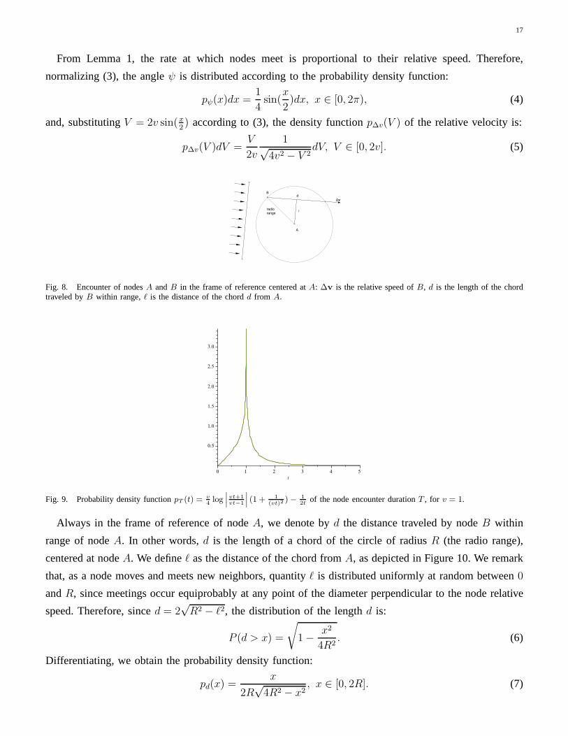
17

From Lemma 1, the rate at which nodes meet is proportional to their relative speed. Therefore,

normalizing (3), the angleψ is distributed according to the probability density function:

pψ(x)dx =1

4sin(

x

2)dx, x ∈ [0, 2π), (4)

and, substitutingV = 2v sin(x2) according to (3), the density functionp∆v(V ) of the relative velocity is:

p∆v(V )dV =V

2v

1√4v2 − V 2

dV, V ∈ [0, 2v]. (5)

Fig. 8. Encounter of nodesA andB in the frame of reference centered atA: ∆v is the relative speed ofB, d is the length of the chordtraveled byB within range,ℓ is the distance of the chordd from A.

t0 1 2 3 4 5

0.5

1.0

1.5

2.0

2.5

3.0

Fig. 9. Probability density functionpT (t) = v

4log

˛

˛

˛

vt+1vt−1

˛

˛

˛(1 + 1

(vt)2) − 1

2tof the node encounter durationT , for v = 1.

Always in the frame of reference of nodeA, we denote byd the distance traveled by nodeB within

range of nodeA. In other words,d is the length of a chord of the circle of radiusR (the radio range),

centered at nodeA. We defineℓ as the distance of the chord fromA, as depicted in Figure 10. We remark

that, as a node moves and meets new neighbors, quantityℓ is distributed uniformly at random between0

andR, since meetings occur equiprobably at any point of the diameter perpendicular to the node relative

speed. Therefore, sinced = 2√R2 − ℓ2, the distribution of the lengthd is:

P (d > x) =

√

1 − x2

4R2. (6)

Differentiating, we obtain the probability density function:

pd(x) =x

2R√

4R2 − x2, x ∈ [0, 2R]. (7)

18

If T is the duration of the encounter, we have:

d = ∆v × T, (8)

where all quantities are random variables.

Let us consider a given relative velocity∆v = V . In this case, we can define the conditional probability

densitypT (t | ∆v = V ) of the encounter duration, witht ∈ [0, 2V

]:

pT (t | ∆v = V )dt = pd(x | ∆v = V )dx = pd(V t)V dt,

wherex = V t, according to (8).

Combining with (7),

pT (t | ∆v = V ) =V 2t

2√

4 − (V t)2. (9)

Considering the probability density functionpT (t), and using (5) and (9), we have fort ≥ 0:

pT (t) =

∫ 2v

0

pT (t | ∆v = V ) × p∆v(V )dV

=1

4log

∣

∣

∣

∣

vRt+ 1

vRt− 1

∣

∣

∣

∣

(

1 +R2

(vt)2

)

− R

2vt.

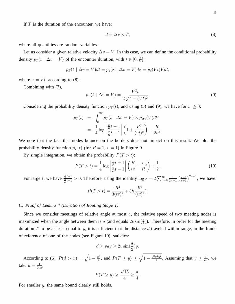
We note that the fact that nodes bounce on the borders does notimpact on this result. We plot the

probability density functionpT (t) (for R = 1, v = 1) in Figure 9.

By simple integration, we obtain the probabilityP (T > t):

P (T > t) =1

4log

∣

∣

∣

∣

vRt+ 1

vRt− 1

∣

∣

∣

∣

(

R

vt− v

Rt

)

+1

2. (10)

For larget, we havev

Rt+1

v

Rt−1

> 0. Therefore, using the identitylog x = 2∑∞

n=01

2n+1

(

x−1x+1

)2n+1, we have:

P (T > t) =R2

3(vt)2+O(

R4

(vt)4).

C. Proof of Lemma 4 (Duration of Routing Stage 1)

Since we consider meetings of relative angle at mosta, the relative speed of two meeting nodes is

maximized when the angle between them isa (and equals2v sin(a2)). Therefore, in order for the meeting

durationT to be at least equal toy, it is sufficient that the distanced traveled within range, in the frame

of reference of one of the nodes (see Figure 10), satisfies:

d ≥ vay ≥ 2v sin(a

2)y.

According to (6),P (d > x) =√

1 − x2

4, andP (T ≥ y) ≥

√

1 − a2v2y2

4. Assuming thaty ≥ 1

vπ, we

takea = 12vy

,

P (T ≥ y) ≥√

15

4≥ π

4.

For smallery, the same bound clearly still holds.

19

Fig. 10. Encounter of nodesA andB in the frame of reference centered atA: ∆v is the relative speed ofB, d is the length of the chordtraveled byB within range,ℓ is the distance of the chordd from A.

From Lemma 1, the probability to meet a node at an angle in[a2, a] is Pa = cos(a

4) − cos(a

2) ≥ 1

16a2,

sincea ≤ π2.

The rate at which a node meets new nodes at such an angle, ensuring that the meeting duration is at

leasty, is:

f1 ≥4vν

πPaP (T ≥ y) ≥ vν

16a2.

We note that the angleφC determines the distancedB of nodeC trajectory from the pointB (see

Figure 1). In fact, it holds:dB = |CB| sinφC . When a node moves,φC varies, whiledB remains unchanged.

In fact φC always increases when a node moves towards the destination.However, after a node movement

of distanceδ, we have∆φC = O( δ|CB|), and if δ = o(|CB|), φC is not modified asymptotically.

Thus, if the initial angle between the source and the destination is b, the expected timeE(t′1) untila2≤ φC ≤ a is:

E(t′1) ≤2b

af≤ 32π

a3vν= Θ(

1

vν).

From Lemma 1, the rate at which a node meets nodes at relative angle [ψ, ψ + dψ] is 2vνπ

sin(β2)dβ.

Therefore, the nodeC that last received the information meets new nodesC ′ with angleφ′C ≤ 1√

r, and

with meeting duration at leasty, with rate (assuming thatφC remains betweena2

anda):

f2 ≥ 2vν

πP (T > y)

∫ a+ 1√

r

a− 1√

r

sin(a

4+ x)dx ≥ vν sin(a

4 )

4√

r+ O(r−

3

2 ).

and the expected timeE(t′′1) until meeting such a node isΘ(√r

vν) (we note that1

a≤ 2K). We notice that

the t′′1 = o(r) almost surely, and we can indeed assume thatφC remains constant until meetingC ′.

Therefore, it holds that the durationt1 of stage 1 ist1 = t′1 + t′′1 = O(√r

vν) almost surely. The distance

traveled isvt1+O( 1a), where the second term corresponds to the further distance moved by the information

in O( 1a) transmissions. Since1

a= O(1), the total distance traveled isO(

√r

ν).

D. Proof of Lemma 7 (Duration of Routing Stage 3)

We proceed equivalently to stage 1. Stage 3 ends when a node with angleφC ≤ 12rC

receives the

information. Equivalently to the proof of Lemma 4, the expected timet′3 until the relative speed of the

node to the rendez-vous pointA is betweena2

anda is E(t′3) = Θ( 1vν

).

20

We consider meetings with nodesC ′, such that2rC′ ≤√r

k1, wherek1 > 0 is a constant. The nodeC

that last received the information meets new nodesC ′ with angleφC′ ≤ k1√r

(≤ 12r

C′

), and with meetingduration at leasty, with rate (assuming thatφC is betweena

2anda):

f2 ≥ 2vν

πP (T > y)

∫ a+k1√

r

a−k1√

r

sin(a

4+ x)dx ≥ k1vν sin(a

4 )

4√

r+ O(r−

3

2 ).

and the expected timeE(t′′3) until meeting such a node isΘ(√r

vν). SinceφC varies, if it becomes larger

thana (or smaller thana2), the information is forwarded to a new node such thatφC is betweena

2anda

again (in constant time).

Moreover, we have indeed thatrC = O(√r) ≤

√r

2k1(1 +O(1)) for some positive constantk1, since the

distance traveled at this stage is at mostvt′3 + vt′′3 + O( 1a) = O(

√r). We assume thatrC ≤ rB, which

we can ensure by choosing pointB sufficiently far from the rendez-vous pointA. In this case, when

the information is transmitted to nodeC, the node’s direction, with respect to the destination’s speed, is

of angle at mostφC ≤ a. Therefore, after timet3 = Θ(√r

vν), the destination is reached with probability

strictly larger than0.

E. Proof of Corollary 1

W. l. o. g., we takeR = 1 andG = 1. Let (ρ, θ(ρ)) be an element of the setK. We have:

θ(ρ) =√

(τ + γ(y)νH(ρ))2 + ρ2v2 − τ, (11)

with

H(ρ) =4πvI0(ρ)

1 − γ(y)πν2ρI1(ρ)

. (12)

For y sufficiently large, such thatγ(y)ν = π2ν8vy

→ 0,

θ(ρ) =√

τ 2 + ρ2v2 − τ +τ

√

τ 2 + ρ2v2H(ρ)

π2ν

8vy+O(

ν2

y2),

and, sinceH(ρ) = 4πvI0(ρ) +O(ν2

y2), we obtain the ratio:

θ(ρ)

ρ=

√

τ 2 + ρ2v2 − τ

ρ+

τ√

τ 2 + ρ2v2I0(ρ)

π3ν

2yρ+O(

ν2

y2ρ).

Therefore, whenρ→ 0,θ(ρ)

ρ=ρv2

2τ+π3ν

2yρ+O(

ν2

y2ρ+νρ2

y)

The sumρv2

2τ+ π3ν

2yρis minimized whenρ = π

v

√

ντy

, and its minimum isπv√

νyτ

.

As a result, the ratioθ(ρ)ρ

is minimized with valueπv√

νyτ

+ O((

νy

)32), which corresponds to the

propagation speed bound.

21

F. Proof of Corollary 2

Again, we take w. l. o. g.,R = 1 andG = 1, and we consider the kernel set(ρ, θ(ρ)). From (11), when

τ → 0,

θ(ρ) =√

(γ(y)νH(ρ))2 + ρ2v2 +O(τ).

We obtain the ratio:θ(ρ)

ρ=

√

(γ(y)νH(ρ))2

ρ2+ v2 +O(

τ

ρ).

In this case,√

(γ(y)νH(ρ))2

ρ2+ v2 is minimized when the quantityJ(ρ) = γ(y)νH(ρ)

ρis also minimized.

We takeγ(y) = π2

8vy, since this is an upper bound for any value of the parameters.Thus, using (12)

when νy→ 0,

J(ρ) =π2νH(ρ)

8vyρ=π2νI0(ρ)

8yρ+O(

ν2

y2).

Therefore, the minimum ofJ(ρ) is π2ν8y

minρ(I0(ρ)ρ

) +O(ν2

y2), attained forρ = 1.608 . . ., and we have the

propagation speed upper bound:v +O(ν2

y2+ τ).